alan calder ([email protected]) sean couch …hipacc.ucsc.edu/lecture...
TRANSCRIPT

1
HIPACC Summer School
July 20, 2011
Alan Calder ([email protected])
Sean Couch ([email protected])
Many, many others!
Explosive Astrophysics with Flash

2
Outline
Introducing Flash
Components of Flash
Running a simulation with Flash
Simulating with Flash
Block Structured AMR
System Requirements
Verification and Validation: definitions and methods
Case studies with Flash
Issues relevant to performing quality simulations.
Sample nuclear astrophysics problems.
2-d cellular detonation
1-d flame
2-d white dwarf detonation
Introducing Flash
Flash has been under development since 1997 at the Flash Center for
Computational Science at the University of Chicago.
Many, many developers.
Current developers: Anshu Dubey (group leader), John Bachan,
Sean Couch, Chris Daley, Milad Fatenejad , Norbert Flocke , Carlo
Graziani, Shravan Gopal , Cal Jordan, Dongwook Lee, Dean
Townsley, Klaus Weide.
Past major developers: Katie Antypas, Alan Calder, Jonathan
Dursi, Robert Fisher, Kevin Olson, Timur Linde, Tomek Plewa, Paul
Ricker, Katherine Riley, Andrew Siegel, Dan Sheeler, Frank
Timmes, Natasha Vladimirova, Greg Weirs, Mike Zingale.
Documentation
http://flash.uchicago.edu/site/flashcode/user_support
3

What is Flash?
4
Flash is composed of units (code modules) that are combined to
construct a code for a particular application.
Flash is written principally in Fortran, with some C and Python. The
physics units are in Fortran.
A setup script performs the steps to construct the code for an
application. It processes information in configuration scripts for a
particular problem and for the units. It also takes arguments.
Flash applications include
Nuclear astrophysics
Cosmology
Fluid dynamics
High energy density physics
5
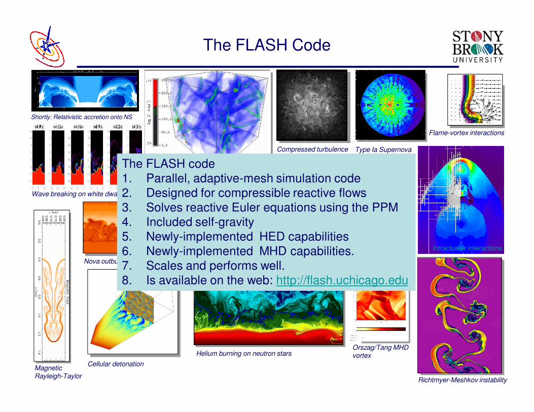
The FLASH Code
Cellular detonation
Compressed turbulence
Helium burning on neutron stars
Richtmyer-Meshkov instability
Laser-driven shock instabilitiesNova outbursts on white dwarfs Rayleigh-Taylor instability
Flame-vortex interactions
Gravitational collapse/Jeans instability
Wave breaking on white dwarfs
Shortly: Relativistic accretion onto NS
Orszag/Tang MHDvortex
Type Ia Supernova
Intracluster interactions
MagneticRayleigh-Taylor
The FLASH code
1. Parallel, adaptive-mesh simulation code
2. Designed for compressible reactive flows
3. Solves reactive Euler equations using the PPM
4. Included self-gravity
5. Newly-implemented HED capabilities
6. Newly-implemented MHD capabilities.
7. Scales and performs well.
8. Is available on the web: http://flash.uchicago.edu

Flash Infrastructure Capabilities
6
Configuration (setup)
Mesh Management
PARAMESH- block structured AMR
Chombo- patch based AMR
Uniform grid
Parallel I/O
HDF 5
PnetCDF
Fortran
Monitoring
Performance monitoring
Verification testing
Unit
Regression

Flash Physics
7
Flash Units:
Hydrodynamics, MHD, RHD
Material equations of state
Nuclear physics and other source terms
Gravity- applied and self-gravitating
Material properties
Cosmology
High energy density
Particles
Lagrangian tracers
Active (massive)

Example: Cellular Detonation Problem
8
Nuclear astrophysics example : a cellular detonation.
Problem described in Timmes et al. ApJ 543 938 (2000)

Running Flash I
9
Move to the project directory
cd /project/projectdirs/training/HIPACC_2011/calder/
Unpack the tar file
tar xzvf FLASH4-alpha
Move to the directory in which the code resides
cd FLASH4-alpha
Run the setup script to set up the cellular detonation problem
./setup Cellular -auto -site=hopper.nersc.gov
Move into the newly-created object directory and compile the code
cd object
make

Running Flash I
10
Important note: One can set many parameters at setup time to
tailor the simulation for the architecture, etc.
An example is maxblocks, which sets the maximum number of
blocks per processor element. Recall Katie Antypas’s point about
the memory per core decreasing from Franklin to Hopper. Must
account for thiis!
./setup Cellular -auto -site=hopper.nersc.gov -
objdir=obj_cellular2 -maxblocks=200
More on estimating the memory utilization later.

Performance Example
11

Adaptive Mesh Refinement
AMR seeks to minimize computational expense by adding resolution
elements only as needed to resolve features in the flow.
Flash uses a block-structured approach to AMR.
The simulation domain is divided into a series of logically-Cartesian
blocks with the resolution set by the number of blocks in a region of
physical space.
The number of blocks changes (adapts) via a parent-child relationship.
The mesh package (e.g. PARAMESH)
Manages the creation of grid blocks
Builds and maintains the tree structure that tracks the spatial
relationship between blocks
Distributes blocks among available processors
Handles inter-block and inter-processor communication.
Tracks physical boundaries and enforces boundary conditions 12

Adaptive Mesh Refinement
13

Adaptive Mesh Refinement
14

Adaptive Mesh Refinement
15

Example Block
16From Fryxell et al. ApJS 131 273 (2000)

Example Domain
17From Fryxell et al. ApJS 131 273 (2000)
Subcycling- Zingale & Dursi
http://xxx.lanl.gov/abs/astro-ph/0310891

Morton Space-filling Curve
18From Fryxell et al. ApJS 131 273 (2000)

Flux Conservation at Block Boundaries
19From Fryxell et al. ApJS 131 273 (2000)
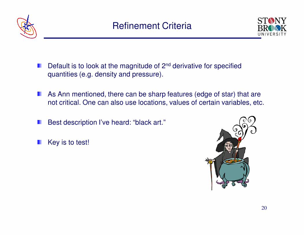
Refinement Criteria
Default is to look at the magnitude of 2nd derivative for specified
quantities (e.g. density and pressure).
As Ann mentioned, there can be sharp features (edge of star) that are
not critical. One can also use locations, values of certain variables, etc.
Best description I’ve heard: “black art.”
Key is to test!
20

Initial Conditions
Very important- When one constructs initial conditions, one writes a
routine to initialize the blocks.
Typical uniform mesh codes perform a loop stuffing arrays over the
whole domain. Initializing a block requires querying its location and
initialize the variables accordingly. This process can be difficult to
conceptualize.
For this Summer School, we will look at three setups relevant to
simulating Type Ia supernovae
cellular detonation
1-d deflagration
2-d detonation in a white dwarf.
Homework assignment: Modify the cellular detonation setup to instead
simulate a 1-d deflagration. (Details below).21

System Requirements for Flash
Compiler for Fortran (F90) and C.
Installed copy of the Message Passing Interface (MPI)
Installed packages for I/O, Hierarchical Data Format (HDF) or Parallel
NetCDF (PnetCDF). There is a Fortran I/O option, but your mileage will
vary.
Flash is distributed with the PARAMESH AMR library included. For
Chombo AMR, one must have the Chombo library included.
For the implicit Diffuse and Hypre solvers, one must have the Hypre
library installed.
GNU make utility.
Python 2.2 or later for the setup script.22

Running Flash II
23
Move into or create the run directory (usually in the scratch space)
mkdir 20110712_cellular
cd 20110712_cellular
Copy the required files into the run directory
cp …/FLASH4-alpha_release/object/SpeciesList.txt .
cp …/FLASH4-alpha_release/object/helm_table.dat .
cp …/FLASH4-alpha_release/object/flash.par .
cp …/FLASH4-alpha_release/object/flash4 .
Copy or create a run script in the run directory
vi (or emacs) hopper.run (example next slide)
Submit the job to the queue:
qsub hopper.run
Monitor the job as you please:
qstat –u username

Example run script for Hopper
24
Example run script:
#PBS -N cellular01
#PBS -q debug
#PBS -l mppwidth=12
#PBS -l walltime=0:29:00
#PBS -e output.$PBS_JOBID.err
#PBS -o output.$PBS_JOBID.out
cd $PBS_O_WORKDIR
echo Starting `date`
aprun -n 12 ./flash4
echo Ending `date`

Operator Splitting
25
The different modules operating on the state are strung together via
Strang spliitting, a fractional step method, in which the operators act
on parts of one time step.
Consider advection + reaction:
Want to solve combined problem:
Solve via
where
From R. LeVeque in “Computational Methods or Astrophysical Fluid Flow”
∆t/2
∆t/2
∆t

Driver Routine Illustrating Strang Splitting
26
do dr_nstep = dr_nbegin, dr_nend
call Hydro( blockCount, blockList, &
dr_simTime, dr_dt, dr_dtOld, dr_fSweepDir)
call RadTrans(blockCount, blockList, dr_dt, pass=1)
call Diffuse(blockCount, blockList, dr_dt, pass=1)
call Driver_sourceTerms(blockCount, blockList, dr_dt, pass=1)
call ravity_potentialListOfBlocks(blockCount,blockList)
call Hydro( blockCount, blockList, &
dr_simTime, dr_dt, dr_dtOld, dr_rSweepDir)
call RadTrans(blockCount, blockList, dr_dt, pass=2)
call Diffuse(blockCount, blockList, dr_dt, pass=2)
call Driver_sourceTerms(blockCount, blockList, dr_dt)
call Gravity_potentialListOfBlocks(blockCount,blockList)
end do

Finite Volume Methods
27
Euler equations :
Conserved quantities:
Volume average
Volume
as volume average of take
From Zingale et al. 2002
Integral form of Euler
equations :

Finite Volume Methods
28
In finite volume methods, the average value of the unknown is
given by
Where xi+1/2, xi-1/2 are the positions of the left, right edges of the
zone.
One performs a reconstruction (piecewise constant, linear,
parabolic, …) to get f(x) and then one integrates that.
Parabolic example is Simpson’s rule (seen for integration)

Area of i+1/2th subinterval
Simpson’s Rule
Approximate area of each
subinterval by area under a
parabola passing through
points f(xi), f(xi+1/2),f(xi+1)
29

Finite Volume Hydrodynamics Methods
Divide the domain into zones the interact with fluxes30

Godunov Method
The original Godunov method solved the Riemann problem at the
boundaries between zones using the average values 31

Piecewise Linear Godunov Methods
Piecewise linear methods perform a linear interpolation.
Higher-order methods exist. PPM is Piecewise-Parabolic Method
32
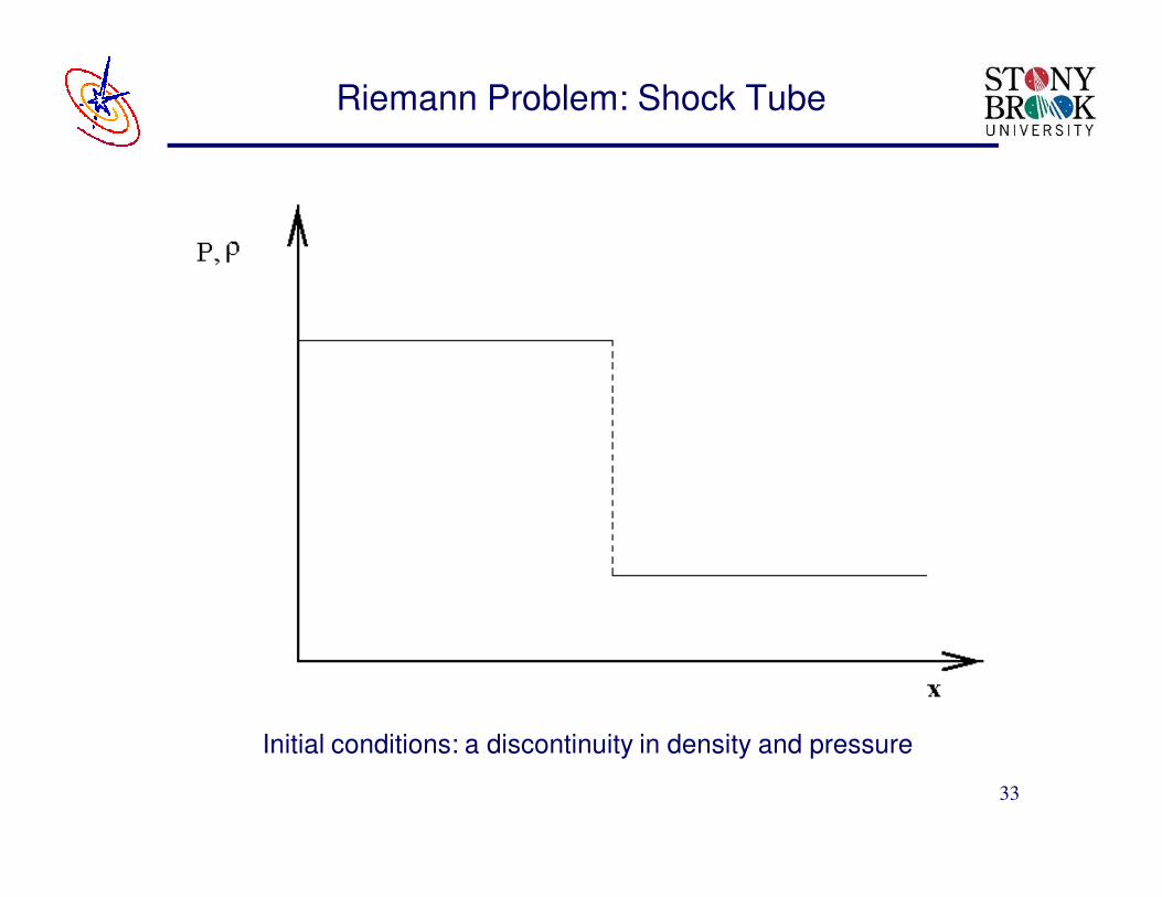
Riemann Problem: Shock Tube
Initial conditions: a discontinuity in density and pressure
33

Riemann Problem: Shock Tube
World diagram for Riemann problem
34

Riemann Problem: Shock Tube
PPM has special algorithms for these features
35

Contact Discontinuity Detection
36
Density profile
that will trigger
special algorithm
From Fryxell, et al. 2000

Contact Steepening Process
37
From Fryxell, et al. 2000

Contact Discontinuity w/ steepening
38
From Fryxell, et al. 2000

Contact Discontinuity w/o steepening
39
From Fryxell, et al. 2000

Intermission
40

V&V Vocabulary
Verification- Determining that the implementation accurately represents the conceptual description of the model.
Quantify error.
Approach is a systematic refinement study (space and time).
Validation- Determining the degree to which a model is an accurate representation of the real world.
Test key elements (modules) and integrated code.
Compare to actual experiments (quantify error).
Calibration- process performed to improve the agreement between simulation and experiment. Not validation!
Prediction- use of the code or model for an application for which it has not been validated.
41

Verification and Validation
Verification: “solving the equations right”
Validation: “solving the right equations”
From Calder, et al. 2002

Our V&V Methodology
Choose V&V tests/problems for particular code modules e.g.
hydrodynamics. Test integrated code also if possible.
Verification test problems
Unit tests
Investigate convergence of error with resolution
Investigate error in secondary modules e.g. EOS
Regularly re-verify with nightly/weekly automated tests
Validation problems
Quantify measurements in experiment and simulation
Quantify error and uncertainty in experiment and simulation
Resolution study (verification-type tests)
Note: astrophysics is largely prediction.
43

Verifiability: The New Test Suite
Flash test suite automatically runs set of verification tests
Essential for identifying bugs unintentionally introduced
New test suite released with FLASH3 so users can monitor their own research problems and performance
test parameters easily modified through GUI
handles unit tests, compilation tests, comparison tests
automatically uploads test suite data to benchmarks database
Green light indicates all
runs were successful
Date of run
Platform
Floating statistics box gives
immediate overview of results
Red light indicates 1 or more
tests failed
44
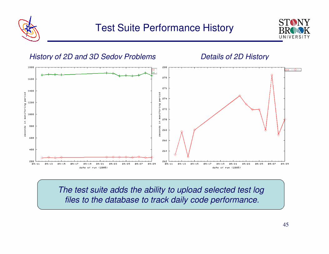
Test Suite Performance History
The test suite adds the ability to upload selected test log
files to the database to track daily code performance.
History of 2D and 3D Sedov Problems Details of 2D History
45
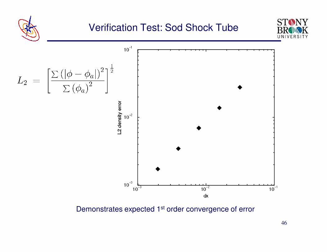
Verification Test: Sod Shock Tube
Demonstrates expected 1st order convergence of error
46
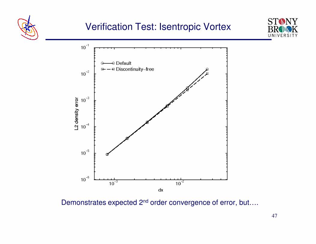
Verification Test: Isentropic Vortex
Demonstrates expected 2nd order convergence of error, but….
47

Sod Tube W/ AMR
Demonstrates expected 1st order convergence of error, but note that the
imperfect mesh refinement criteria degrades the solution!48

Rayleigh-Taylor Instabilities
g
Lighter fluid
2.5-5 % sound speed with highest
magnitude near the interface
Denser fluid
Multi-mode velocity perturbation:Density schematic:
49

Multi-mode Rayleigh-Taylor
Organized by G. Dimonte (Oct. 1998)
Purpose – to determine if the t2 scaling law holds for the growth of the
RT mixing layer, and if so, to determine the value of α
simulation - experiment comparisons
inter-simulation comparisons
hb,s = αb,s gAt2, where A = (ρ2 - ρ1)/ (ρ2 + ρ1)
Definition of standard problem set (D. Youngs)
Dimonte et al. Phys. Fluids 16 1668 (2004)
“α-Group” Consortium
50

Multi-mode Rayleigh-Taylor: 2-d Simulation
51

Multi-mode Rayleigh-Taylor: 3-d Simulation
Horizontally Averaged Density
Modes 32-64 perturbed
52

Multi-mode Rayleigh-Taylor: Inverse Cascade
Bubbles of the lighter fluid in the denser fluid
t = 7.00 sec t = 14.75 sec
53

Multi-mode Rayleigh-Taylor
Density (g/cm3) at t = 14.75 sec
Rendering of
Mixing Zone
54

Multi-mode R-T Experimental LIF Image
It looks similar to the simulation…..
55

Multi-mode R-T Simulated LIF Image
It looks similar to the experiment…..
56

Multi-mode Rayleigh-Taylor
FLASH Simulation
αbubble = 0.021
αspike = 0.026
57
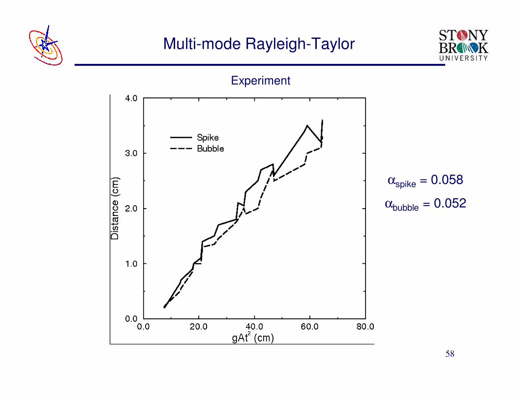
Multi-mode Rayleigh-Taylor
Experiment
αbubble = 0.052
αspike = 0.058
58

Single-mode 3-D Rayleigh-Taylor
Density (g/cc)4 8 16 32 64 128
λ (grid points)t = 3.1 sec
256
59
Flash Exercises
Set up and run the cellular detonation problem. Visualize the results
with VisIt.
Investigate differences between hydrodynamics solvers for the case of
the Kelvin-Helmholtz instability.
Two SN Ia related problems- thermonuclear flame and a detonation in
a white dwarf.
60

Thermonuclear Flame Setup
61
Homework assignment: Starting with the Cellular detonation problem
setup, modify it to simulate a deflagration.
Hints:
What resolution?
How is a deflagration different from a detonation? More on this in
the next lecture.
Only two files to modify:
Simulation_initBlock.F90
flash.par
Will need to use the (explicit) diffusion module. Do so with an
option to the setup command.
-with-unit=physics/Diffuse/DiffuseFluxBased

White Dwarf Detonation Setup
Example of setting up a white dwarf model with a detonation.
Hydro + burning + self-gravity.
Test: Turn off burning. How long will the code hold the model steady?
Note that there may be issues!
Name of setup is SnDet.
./setup SnDet -2d -auto -nxb=16 -nyb=16 +cylindrical
-objdir=obj_SnDet
Problem directories are in source/Simulation/SimulationMain
62

63
…and that leads us to
QUESTIONS AND DISCUSSION