algebraic manipulation of scientific datasets
TRANSCRIPT
Noname manuscript No.(will be inserted by the editor)
Algebraic Manipulation of Scientific Datasets
Bill Howe, David Maier
Department of Computer Science, Portland State University, Portland, Oregon, email: {howe, maier}@cs.pdx.edu
The date of receipt and acceptance will be inserted by the editor
Abstract We investigate algebraic processing strate-gies for large numeric datasets equipped with a possiblyirregular grid structure. Such datasets arise, for exam-ple, in computational simulations, observation networks,medical imaging, and 2-D and 3-D rendering. Existingapproaches for manipulating these datasets are incom-plete: The performance of SQL queries for manipulatinglarge numeric datasets is not competitive with special-ized tools. Database extensions for processing multidi-mensional discrete data can only model regular, rectilin-ear grids. Visualization software libraries are designed toprocess arbitrary gridded datasets efficiently, but no al-gebra has been developed to simplify their use and affordoptimization. Further, these libraries are data dependent– physical changes to data representation or organiza-tion break user programs. In this paper, we present analgebra of gridfields for manipulating arbitrary griddeddatasets, algebraic optimization techniques, and an im-plementation backed by experimental results. We com-pare our techniques to those of spatial databases and vi-sualization software libraries, using real examples froman Environmental Observation and Forecasting System.We find that our approach can express optimized plansinaccessible to other techniques, resulting in improvedperformance with reduced programming effort.
1 Introduction
Many scientific datasets can be characterized by the topo-logical structure, or grid, over which they are defined.For example, a timeseries might be defined over a 1-dimensional (1-D) grid, while the solution to a partialdifferential equation using a finite-element method mightbe defined over a 3-dimensional (3-D) grid.
These datasets consist of data tuples bound to thecells of a grid. A grid may possess cells of many dimen-sions; data can be associated with the nodes (0-cells),edges (1-cells), polygons (2-cells), and so on. Figure 1
����� ������ �� ������ �
����� ������ ��� !"$#&% '
(�)�* +,�-�. /0�1 23�4�5 6
7�8�9�:;�<�= >?�@ AB�C�D E
FHGJILKMONQPSRTU
V�W XY�Z�[ \
]_^ `a�b�c�d
e�f ghQiJj kl�m�npoqHrSs&t
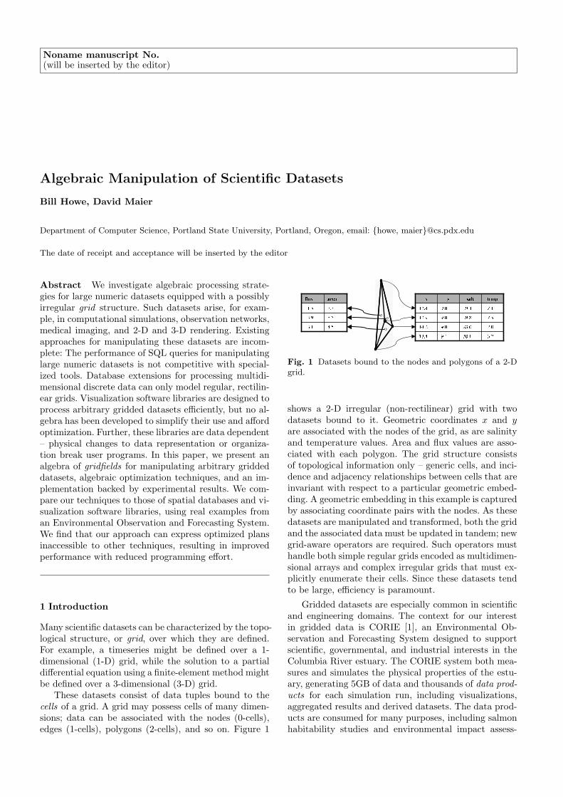
Fig. 1 Datasets bound to the nodes and polygons of a 2-Dgrid.
shows a 2-D irregular (non-rectilinear) grid with twodatasets bound to it. Geometric coordinates x and yare associated with the nodes of the grid, as are salinityand temperature values. Area and flux values are asso-ciated with each polygon. The grid structure consistsof topological information only – generic cells, and inci-dence and adjacency relationships between cells that areinvariant with respect to a particular geometric embed-ding. A geometric embedding in this example is capturedby associating coordinate pairs with the nodes. As thesedatasets are manipulated and transformed, both the gridand the associated data must be updated in tandem; newgrid-aware operators are required. Such operators musthandle both simple regular grids encoded as multidimen-sional arrays and complex irregular grids that must ex-plicitly enumerate their cells. Since these datasets tendto be large, efficiency is paramount.
Gridded datasets are especially common in scientificand engineering domains. The context for our interestin gridded data is CORIE [1], an Environmental Ob-servation and Forecasting System designed to supportscientific, governmental, and industrial interests in theColumbia River estuary. The CORIE system both mea-sures and simulates the physical properties of the estu-ary, generating 5GB of data and thousands of data prod-ucts for each simulation run, including visualizations,aggregated results and derived datasets. The data prod-ucts are consumed for many purposes, including salmonhabitability studies and environmental impact assess-
2 Bill Howe, David Maier
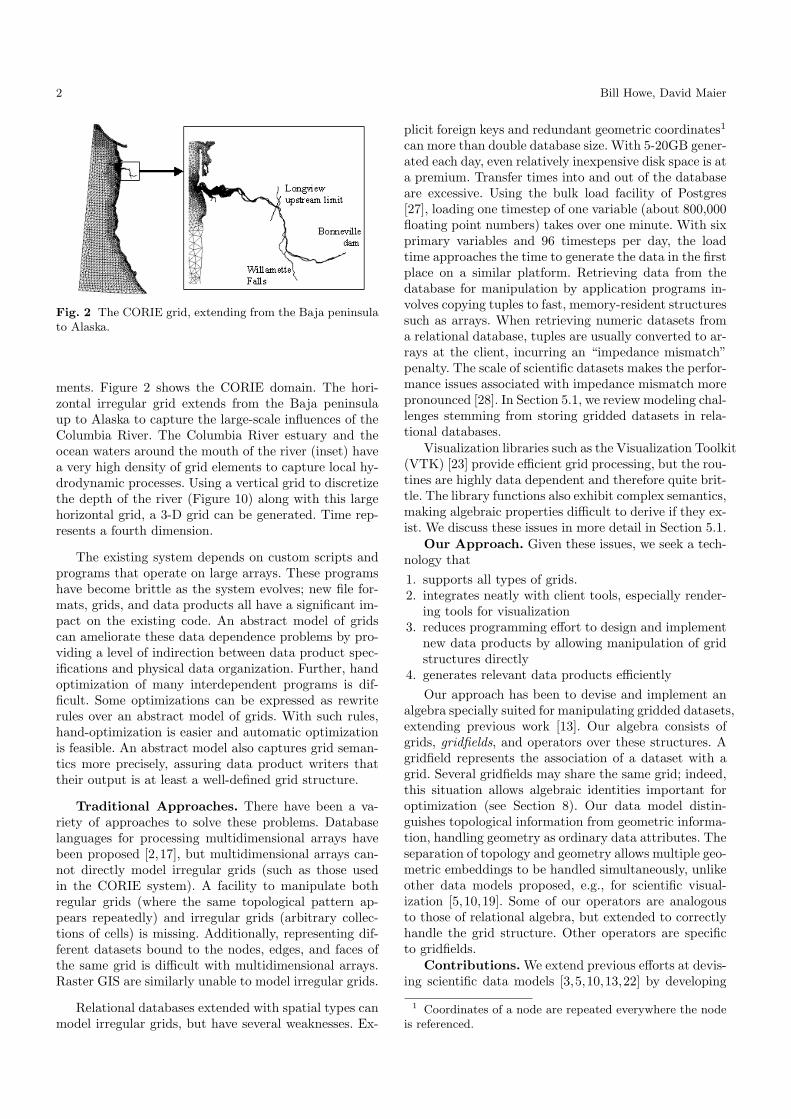
Fig. 2 The CORIE grid, extending from the Baja peninsulato Alaska.
ments. Figure 2 shows the CORIE domain. The hori-zontal irregular grid extends from the Baja peninsulaup to Alaska to capture the large-scale influences of theColumbia River. The Columbia River estuary and theocean waters around the mouth of the river (inset) havea very high density of grid elements to capture local hy-drodynamic processes. Using a vertical grid to discretizethe depth of the river (Figure 10) along with this largehorizontal grid, a 3-D grid can be generated. Time rep-resents a fourth dimension.
The existing system depends on custom scripts andprograms that operate on large arrays. These programshave become brittle as the system evolves; new file for-mats, grids, and data products all have a significant im-pact on the existing code. An abstract model of gridscan ameliorate these data dependence problems by pro-viding a level of indirection between data product spec-ifications and physical data organization. Further, handoptimization of many interdependent programs is dif-ficult. Some optimizations can be expressed as rewriterules over an abstract model of grids. With such rules,hand-optimization is easier and automatic optimizationis feasible. An abstract model also captures grid seman-tics more precisely, assuring data product writers thattheir output is at least a well-defined grid structure.
Traditional Approaches. There have been a va-riety of approaches to solve these problems. Databaselanguages for processing multidimensional arrays havebeen proposed [2,17], but multidimensional arrays can-not directly model irregular grids (such as those usedin the CORIE system). A facility to manipulate bothregular grids (where the same topological pattern ap-pears repeatedly) and irregular grids (arbitrary collec-tions of cells) is missing. Additionally, representing dif-ferent datasets bound to the nodes, edges, and faces ofthe same grid is difficult with multidimensional arrays.Raster GIS are similarly unable to model irregular grids.
Relational databases extended with spatial types canmodel irregular grids, but have several weaknesses. Ex-
plicit foreign keys and redundant geometric coordinates1
can more than double database size. With 5-20GB gener-ated each day, even relatively inexpensive disk space is ata premium. Transfer times into and out of the databaseare excessive. Using the bulk load facility of Postgres[27], loading one timestep of one variable (about 800,000floating point numbers) takes over one minute. With sixprimary variables and 96 timesteps per day, the loadtime approaches the time to generate the data in the firstplace on a similar platform. Retrieving data from thedatabase for manipulation by application programs in-volves copying tuples to fast, memory-resident structuressuch as arrays. When retrieving numeric datasets froma relational database, tuples are usually converted to ar-rays at the client, incurring an “impedance mismatch”penalty. The scale of scientific datasets makes the perfor-mance issues associated with impedance mismatch morepronounced [28]. In Section 5.1, we review modeling chal-lenges stemming from storing gridded datasets in rela-tional databases.
Visualization libraries such as the Visualization Toolkit(VTK) [23] provide efficient grid processing, but the rou-tines are highly data dependent and therefore quite brit-tle. The library functions also exhibit complex semantics,making algebraic properties difficult to derive if they ex-ist. We discuss these issues in more detail in Section 5.1.
Our Approach. Given these issues, we seek a tech-nology that1. supports all types of grids.2. integrates neatly with client tools, especially render-
ing tools for visualization3. reduces programming effort to design and implement
new data products by allowing manipulation of gridstructures directly
4. generates relevant data products efficientlyOur approach has been to devise and implement an
algebra specially suited for manipulating gridded datasets,extending previous work [13]. Our algebra consists ofgrids, gridfields, and operators over these structures. Agridfield represents the association of a dataset with agrid. Several gridfields may share the same grid; indeed,this situation allows algebraic identities important foroptimization (see Section 8). Our data model distin-guishes topological information from geometric informa-tion, handling geometry as ordinary data attributes. Theseparation of topology and geometry allows multiple geo-metric embeddings to be handled simultaneously, unlikeother data models proposed, e.g., for scientific visual-ization [5,10,19]. Some of our operators are analogousto those of relational algebra, but extended to correctlyhandle the grid structure. Other operators are specificto gridfields.
Contributions. We extend previous efforts at devis-ing scientific data models [3,5,10,13,22] by developing
1 Coordinates of a node are repeated everywhere the nodeis referenced.
Algebraic Manipulation of Scientific Datasets 3
algebraic optimizations at both the logical and physicallevels. We contribute a novel data model and implemen-tation that satisfies the goals above. Specifically:1. The data model captures regular and irregular grids
uniformly, and promotes them to first-class citizens.2. We formalize intuitive properties of well-formed grids.3. The design is well-aligned with client visualization
and analysis tools.4. We present alternative representations of grids and
gridfields and discuss the relevant tradeoffs.5. Our operators admit algebraic identities and conse-
quent optimization techniques unique to gridfields.6. We provide experimental evidence of improved per-
formance using a real application: the CORIE simu-lation system.In this paper, we discuss the gridfield model, then
describe data representation, operator implementation,and algebraic optimization of gridfield recipes, a form ofquery plan. Finally, we validate our work via experimen-tal comparisons with existing approaches.
2 Related Work
The database community has given multidimensionaldiscrete data (MDD) significant attention over the pastdecade. OLAP systems have been extended with multi-resolution visualization capabilities [25], but modelingand querying irregular grids in a relational system isdifficult, as we demonstrate later. Query languages andprocessing techniques based on multidimensional arrays[6,16,17,30] have been developed, but arrays are not thecorrect abstraction for general grid manipulations.
Multidimensional arrays capture only rectilinear grids.If, as in the CORIE system, cells in a particular gridmay be triangles, quadrilaterals, or a mix of cell types,the grid structure is awkward to encode using arrays.The interpretation of an assembly of arrays as an ir-regular grid is left to the application, undermining dataindependence. Further, we encounter multiple datasetsbound to the same grid, but perhaps to cells of differentdimension. Using arrays, the relationship between thesedatasets is lost; each must use its own distinct “spa-tial domain” [2] For example, to encode the dataset inFigure 1, we eould need to define two unrelated spatialdomains – one for the 0-cells and one for the 2-cells.The relationship between them is not captured. Finally,the topology suggested by these grids is always implicit,making it difficult to separate geometry from topology.This capability is required when attempting to supporttwo geometric embeddings of the same grid simultane-ously, e.g., in different coordinate systems. Since not alltypes of grids are supported, and grids are cannot bemanipulated directly, our goals 1. and 2. are not met bythese systems.
Several higher-level data models for scientific datahave been proposed that capture both regular and irreg-ular grids, and some separate topology from geometry
[3,5,10]. However, algebraic manipulation of grid struc-tures is not supported and experimental results are notreported, so it is not clear that are efficiency require-ments can be met (goal 4).
Others have demonstrated that relational databasesdo not scale up to handle large scientific datasets [20,26]. One proposed solution is to treat scientific datasetsas external data sources, and access them using the SQLstandard for management of external data (SQL-MED)[18]. Papiani et al. [21] report some success applying thestandard to manage turbulence simulations, though grid-ded datasets are not directly modeled.
Designers of spatial database systems are becomingaware that topological “connection” information can beas important as geometry for modeling and query pro-cessing. ESRI’s ArcGIS version 8.3 [7] includes topologyinformation modeled as integrity rules. Users can expressthe rule that every polygon representing a building mustbe explicitly connected to a line segment representing aroad. ESRI’s product also supports raster data manipu-lation using a Map Algebra, but irregular grids are dif-ficult to model precisely as raster data. Laser-Scan hasproduced a topology-enabled GIS extension for Oraclecalled Radius [29]. They allow nodes to be snapped to-gether to express topological relationships independentlyof geometric embeddings. However, there is no notion ofa manipulable gridded dataset, and therefore, our Goals2 and 3 are not met.
3 Grids
Grids are constructed from sets of cells of various dimen-sion connected by an incidence relationship. We refer toa cell of dimension k as a k-cell, following the topologyliterature [3]. Intuitively, a 0-cell is a point, a 1-cell isa line segment (or poly-line), a 2-cell is a polygon, andso on. These geometric interpretations of cells guide in-tuition, but a grid does not explicitly indicate its cells’geometry.
Our grid model affords interpretation in terms ofwell-studied concepts from topology, particularly cellu-lar complexes (c.f. Fitsch and Piccinini [8]). However, wehave made an effort to avoid strict dependence on theseideas, for two reasons. First, very little of the mathe-matics of topology is directly implementable in the com-puter without a suitable representation theory. Second,the management of data bound to topological structuresrequires a different set of tools than the topology fieldhas to offer; the database community has significant ex-perience designing such tools and their results should beintegrated where possible.
We point out to readers of our previous work on thissubject [12] that we have incorporated significant gener-alizations of the model. What follows is not just a changeof notation, but a change of structure.
Let S be a universe of featureless cells. Let dim be afunction S → N assigning a non-negative integer di-
4 Bill Howe, David Maier
0
1 2A
y
xz
A
x y z
1 2 0
({0,1,2,x,y,z,A},
{(0,0), (0,x), (0,z), (0,A), (1,1), (1,x), (1,y), (1,A), (2,2), (2,y), (2,z), (2,A), (x,x), (x,A), (y,y), (y,A), (z,z), (z,A), (A,A)})
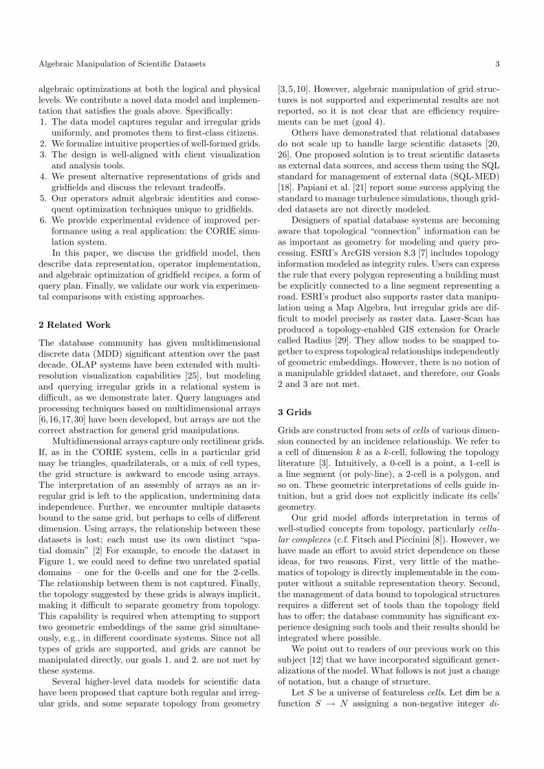
Fig. 3 Hasse diagrams are isomorphic to grids, but many ofour illustrations are not.
mension to each cell in S. Then a grid G is a pair(X,�) where X is a finite subset of S, and � is anincidence relation. Intuitively, the incidence relation en-codes which lower-dimensional cells “touch” a higher-dimensional cell. An incidence relation is a partial orderon X that respects dimension. Specifically, x � y, read“x is incident to y,” implies that either dim(x) < dim(y)or that x = y, so that two distinct cells with the samedimension cannot be incident to each other. We also de-fine ≺ to be the anti-reflexive restriction of �. If twocells x and y of the same dimension share an incidentcell z, then we say that x is adjacent to y. Given a gridG = (X,�G), we will write Gk to indicate the cells inX of a particular dimension k. That is, Gk = {x | x ∈X, dim(x) = k}. We define the dimension of a grid G,written dim(G), as max(dim(x)) over all x ∈ X. Notethat for a d-dimensional grid, Gd must be non-empty,but Gi may be empty for 0 ≤ i < d.
In Figure 1, the grid has four 0-cells, six 1-cells, andthree 2-cells, and it therefore has dimension 2. The inci-dence relation suggested by the figure makes each nodeincident to some edges, each edge incident to one or moretriangular faces, and by the transitivity of a partial or-der, each node also incident to one or more faces.
This definition is very general; a grid may be a col-lection of unconnected polygons for GIS data, a set ofscattered points for values of a random variable, or awell-connected graph modeling the truss structure of abridge. The grids in our application are used to discretizethe Columbia River estuary, for solving the 3-D trans-port equations via a finite-element method.
In our illustrations, we will use draw nodes as blackpoints, 1-cells as line segments, and 2-cells as shadedregions. From these kinds of pictures, we can unambigu-ously derive a grid by creating a cell for each drawingcomponent, and establishing an incidence relationshipbetween cells if they touch in the drawing and their di-mensions are different. However, we cannot unambigu-ously derive a drawing from an arbitrary grid. Since wemodel complex topological structures with little morethan a partial order, the richest visualization of a gridwe can create is a Hasse diagram. A Hasse diagram is adirected graph representation of a partial order. We use aHasse diagram to express the incidence relationship; ver-tices are cells and edges are drawn to indicate incidencerelationships that cannot be derived through the transi-tive closure. Further, vertices are organized into rows ofequal dimension. Figure 3 illustrates the situation.
z0
1
2
yxF =
z
0
1
2
y
xE =
E ∩∩∩∩ F =z
0
1
2
y
x
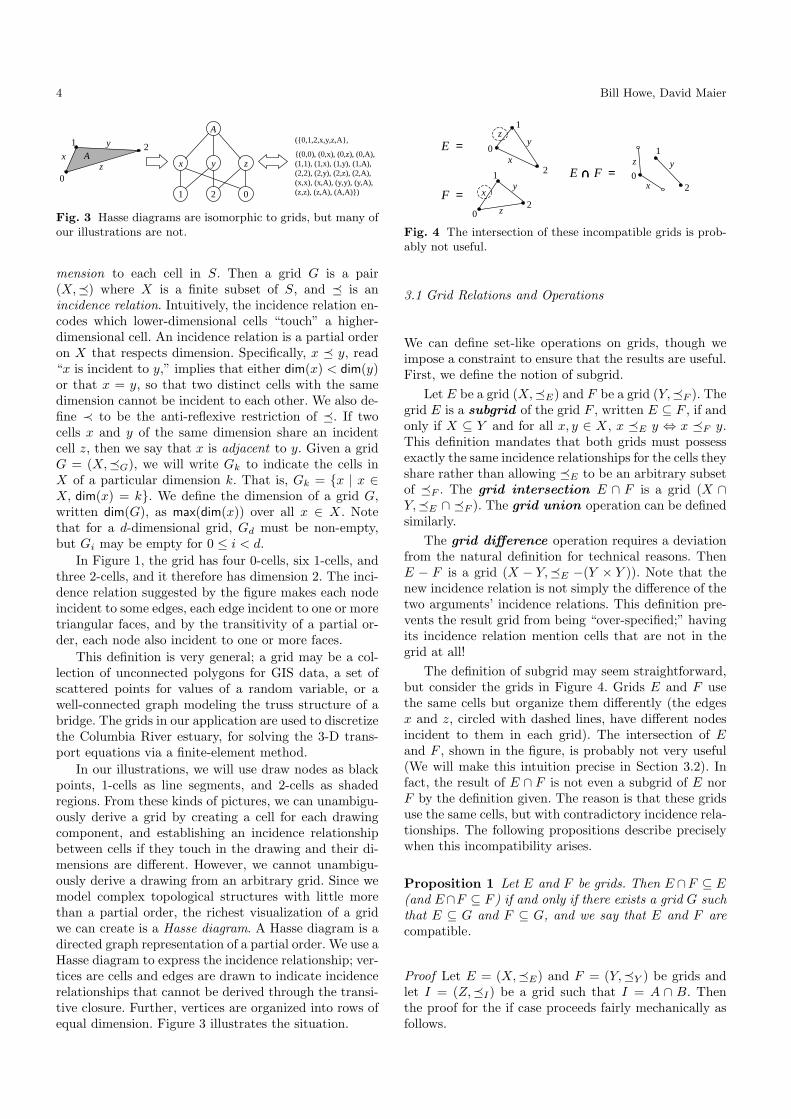
Fig. 4 The intersection of these incompatible grids is prob-ably not useful.
3.1 Grid Relations and Operations
We can define set-like operations on grids, though weimpose a constraint to ensure that the results are useful.First, we define the notion of subgrid.
Let E be a grid (X,�E) and F be a grid (Y,�F ). Thegrid E is a subgrid of the grid F , written E ⊆ F , if andonly if X ⊆ Y and for all x, y ∈ X, x �E y ⇔ x �F y.This definition mandates that both grids must possessexactly the same incidence relationships for the cells theyshare rather than allowing �E to be an arbitrary subsetof �F . The grid intersection E ∩ F is a grid (X ∩Y,�E ∩ �F ). The grid union operation can be definedsimilarly.
The grid difference operation requires a deviationfrom the natural definition for technical reasons. ThenE − F is a grid (X − Y,�E −(Y × Y )). Note that thenew incidence relation is not simply the difference of thetwo arguments’ incidence relations. This definition pre-vents the result grid from being “over-specified;” havingits incidence relation mention cells that are not in thegrid at all!
The definition of subgrid may seem straightforward,but consider the grids in Figure 4. Grids E and F usethe same cells but organize them differently (the edgesx and z, circled with dashed lines, have different nodesincident to them in each grid). The intersection of Eand F , shown in the figure, is probably not very useful(We will make this intuition precise in Section 3.2). Infact, the result of E ∩ F is not even a subgrid of E norF by the definition given. The reason is that these gridsuse the same cells, but with contradictory incidence rela-tionships. The following propositions describe preciselywhen this incompatibility arises.
Proposition 1 Let E and F be grids. Then E ∩F ⊆ E(and E∩F ⊆ F ) if and only if there exists a grid G suchthat E ⊆ G and F ⊆ G, and we say that E and F arecompatible.
Proof Let E = (X,�E) and F = (Y,�Y ) be grids andlet I = (Z,�I) be a grid such that I = A ∩ B. Thenthe proof for the if case proceeds fairly mechanically asfollows.

Algebraic Manipulation of Scientific Datasets 5
E ⊆ G and F ⊆ G
⇒∀x, y ∈ X, x �E y ⇔ x �G y
and ∀x, y ∈ Y , x �F y ⇔ x �G y
⇒∀x, y ∈ X ∩ Y , (x �E y ⇔ x �G y)and (x �F y ⇔ x �G y)
⇔∀x, y ∈ X ∩ Y , (x �E y ⇔ x �G y)and (x �E y and x �F y ⇔ x �G y)
⇔∀x, y ∈ X ∩ Y , (x �E y and x �F y ⇔ x �E y)
The last line, together with the fact that X ∩ Y ⊆ Y ,proves that E ∩ F ⊆ E.
For the only if case, we assume that E ∩ F ⊆ Eand E ∩ F ⊆ F and construct a grid G = (X ∪ Y,�G),where for all x, y ∈ X, x �G y ⇔ x �E y and for allx, y ∈ Y − X, x �G y ⇔ x �F y. Since the incidencerelation of the intersection grid agrees with E and Ffor the cells they share, then the incidence relation of Gwill agree with E and F everywhere. Then no “incidenceconflicts” arise, and E ⊆ G and F ⊆ G.
We omit similar proofs for the following two propo-sitions.
Proposition 2 Let E and F be grids. Then E ⊆ E ∪F(and F ⊆ E ∩F ) if and only if E and F are compatible.
Proposition 3 Let E and F be grids. Then E−F ⊆ Eif and only if E and F are compatible.
The significance of these propositions is that gridscan be combined in meaningful ways only if there is areference grid of which they are all subgrids. Withoutthis constraint, two different applications may organizethe same cells in different ways, resulting in incompatiblegrids. This constraint is fairly intuitive in practice. TheCORIE application for example has made use of severaldistinct grids to describe the same geometric space onthe Earth’s surface as algorithms are refined and tested,new compute platforms are deployed, and different phe-nomena are studied. As a result of these propositions,we can deduce that computing the union or intersectionof these grids is likely meaningless. In order to comparedata on two incompatible grids, we must first assign thecells of one grid to the cells of another grid explicitly.Reasonable assignments might depend on geometry orother external data, rather than the topology alone. InSection 4.1, we describe the aggregate operator that im-plements such assignments.
3.1.1 Cross product. The cross product operator canbe used to produce a higher-dimensional grid from twolower- dimensional grids. The definition of grid crossproduct involves the notion of pairs of cells. Specifi-cally, we assume that for cells x and y in the universe S,the pair (x, y) is also a cell in S. Further, dim((x, y)) =
2
3 4E =
0
1
A 20
30
40
21
31
41
G = E ⊗ F
F =
y
xz
w
2w 4w
z1
z0
x0 y0A0
A1x1 y1
zw
ywxw
Aw
3w
Fig. 5 The cross product of two simple grids.
dim(x) + dim(y). This rule tells us that the product oftwo nodes is another node (0 + 0 = 0), the product ofan edge and another edge is (informally) a quadrilateral(1 + 1 = 2), and so on. In our discussion, we will writexy for the pair (x, y).
Figure 5 shows an example of the cross product op-eration. The cross product of grids E and F contains six0-cells, nine 1-cells, five 2-cells, and one 3-cell. The 3-cellis the interior of the prism, the 2-cells are the three rect-angular faces and the two triangular bases, the 1-cellsare the edges, and the 0-cells are the nodes.
The 3-cell prism in G is just the pair Aw. Geometri-cally, this prism is generated by sweeping the triangle Athrough a third dimension defined by the line segmentw. This geometric interpretation of the cross product op-eration is instructive, but is not formally a part of thegrid definition. All we know about the prism is encodedin the explicit incidence relation between its constituentcells. For example, the figure suggests that in the resultgrid G, the 1-cell x0 is incident to the 2-cells A0 and xw.This makes sense, since in the grid E, the 1-cell x wasincident to the 2-cell A, and in the grid F , the node 0was incident to the 1-cell w.
We can further explain the intuition behind crossproduct by considering one dimension at a time. Thecells of G, by dimension, are given by
G0 = E0 × F0
G1 = (E1 × F0) ∪ (E0 × F1)G2 = (E2 × F0) ∪ (E1 × F1)G3 = E2 × F1
Evaluating these expressions, we obtain
G0 = {20, 30, 40, 21, 31, 41}G1 = {x0, y0, z0, x1, y1, z1, 2w, 3w, 4w}G2 = {A0, A1, xw, yw, zw}G3 = {Aw}
In general, let E = (X,�E) and F = (Y,�F ) be grids,and let d = dim(E) + dim(F ). The cross product of Eand F , written E ⊗F , is a grid G = (X × Y,�G) whereac �G bd if and only if a �E b and c �F d. The cellsof G for a particular dimension k are given by Gk =⋃k
j=0 Xj × Yk−j for 0 ≤ k ≤ d.We have used the cross product operator frequently
in expressing the data products of the CORIE system.
6 Bill Howe, David Maier
y0
1x
A
i)0
1
x y
ii)
z0
1
2
3
yx
w
A
iii)
0A
iv)
x
0
12
v)
z
yx
0
1
2
vi)
0
1
2
3zy
xvii)
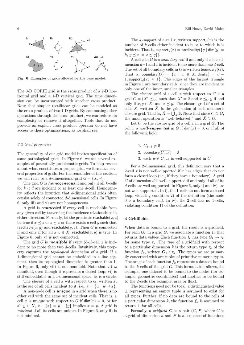
Fig. 6 Examples of grids allowed by the base model.
The 3-D CORIE grid is the cross product of a 2-D hor-izontal grid and a 1-D vertical grid. The time dimen-sion can be incorporated with another cross product.Note that simpler rectilinear grids can be modeled asthe cross product of two 1-D grids. By commuting otheroperations through the cross product, we can reduce itscomplexity or remove it altogether. Tools that do notprovide an explicit cross product operator do not haveaccess to these optimizations, as we shall see.
3.2 Grid properties
The generality of our grid model invites specification ofsome pathological grids. In Figure 6, we see several ex-amples of potentially problematic grids. To help reasonabout what constitutes a proper grid, we formalize sev-eral properties of grids. For the remainder of this section,we will refer to a d-dimensional grid G = (X,�).
The grid G is homogeneous if and only if all k-cellsfor k < d are incident to at least one d-cell. Homogene-ity reflects the intuition that d-dimensional grids oftenconsist solely of connected d-dimensional cells. In Figure6, only iii) and v) are not homogeneous.
A grid is connected if every cell is reachable fromany given cell by traversing the incidence relationships ineither direction. Formally, let the predicate reachable(x, z)be true if x � z or z � x or there exists a cell y such thatreachable(x, y) and reachable(y, z). Then G is connectedif and only if for all x, y ∈ X, reachable(x, y) is true. InFigure 6, only v) is not connected.
The grid G is manifold if every (d-1)-cell x is inci-dent to no more than two d-cells. Intuitively, this prop-erty captures the topological dimension of a grid. If a1-dimensional grid cannot be embedded in a line seg-ment, then its topological dimension is greater than 1.In Figure 6, only vii) is not manifold. Note that vi) ismanifold, even though it represents a closed loop; vi) isstill embeddable in a 1-dimensional space, as is a circle.
The closure of a cell x with respect to G, written x,is the set of all cells incident to it; i.e., x = {w | w � x}.
A non-node cell is unique in a grid when there is noother cell with the same set of incident cells. That is, acell x is unique with respect to G if dim(x) = 0, or forall y ∈ X, x − {x} = y − {y} implies x = y. A grid isminimal if all its cells are unique. In Figure 6, only ii) isnot minimal.
The k-support of a cell x, written supportk(x) is thenumber of k-cells either incident to it or to which it isincident. That is, supportk(x) = cardinality({y | dim(y) =k, y � x or x � y}).
A cell x in G is a boundary cell if and only if x has di-mension d−1 and x is incident to no more than one d-cell.The set of all boundary cells in G is written boundary(G).That is, boundary(G) = {x | x ∈ X, dim(x) = d −1, supportd(x) ≤ 1}. The edges of the largest trianglein Figure 1 are boundary cells, since they are incident toonly one of the inner, smaller triangles.
The closure grid of a cell x with respect to G is agrid C = (X ′,�C) such that X ′ = x and x �C y if andonly if x, y ∈ X ′ and x � y. The closure grid of a set ofcells X, written X, is the grid union of each member’sclosure grid. That is, X =
⋃X x. Note that since C ⊆ G,
the union operation is “well-behaved,” and X ⊆ G.Let C be the closure grid of a cell x in a grid G. The
cell x is well-supported in G if dim(x) = 0, or if all ofthe following hold:
1. Cd−1 6= ∅2. boundary(Cd−1) = ∅3. each w ∈ Cd−1 is well-supported in C
For a 2-dimensional grid, this definition says that a2-cell x is not well-supported if x has edges that do notform a closed loop (i.e., if they have a boundary). A gridG of dimension d is well-supported if and only if all of itsd-cells are well-supported. In Figure 6, only i) and iv) arenot well-supported. In i), the 1-cells do not form a closedloop, violating condition 2) of the definition (the node0 is a boundary cell). In iv), the 2-cell has no 1-cells,violating condition 1) of the definition.
4 Gridfields
When data is bound to a grid, the result is a gridfield.For each Gk in a grid G, we associate a function fk thatreturns data values. Each function fk has type Gk → τk
for some type τk. The type of a gridfield with respectto a particular dimension k is the return type τk of thefunction fk, written Gk : τk. The types we are primar-ily concerned with are tuples of primitive numeric types.The range of each function fk represents a dataset boundto the k-cells of the grid G. This formulation allows, forexample, one dataset to be bound to the nodes (for ex-ample, geometric coordinates) and another to be boundto the 2-cells (for example, area or flux).
The functions need not be total; a distinguished value⊥ representing an empty tuple is assumed to exist forall types. Further, if no data are bound to the cells ofa particular dimension k, the function fk is assumed toreturn ⊥ for all cells.
Formally, a gridfield G is a pair (G,F) where G isa grid of dimension d and F is a sequence of functions
Algebraic Manipulation of Scientific Datasets 7
a) c)b)
Fig. 7 Three different geometric realizations of the sametopological grid.
(g0, . . . , gd), one for each dimension i. We will typicallycollapse the pair structure and just write (G, g0, . . . , gd).
Given a gridfield G = (G, g0, . . . , gd), we define helperfunctions grid(G) = G, and dataset(G, i) = {gi(x) |x ∈ Gi}. We will refer to the result of the latter functionas the “dataset at rank i”. We can also extract the se-quence of functions (g0, . . . , gd) that bind data values tocells by writing bindings(G). Given a function f : Gk →(τ0, . . . , τn) and a function g : Gk → (υ0, . . . , υm) wedefine the concatenation of f and g, written f g, as afunction returning tuples of type (τ0, . . . , τn, υ0, . . . , υm)such that the tuples returned by f and g are concate-nated together.
Earlier we used a trussed bridge as an example of agrid. A gridfield defined over such a grid might returnthe net force at each node and the linear force alongeach truss. A gridfield can capture both cases by bindingdata to G0 and G1, respectively. Images can be viewednaturally as data bound to the 2-cells of a rectilinearproduct grid. We can also model unstructured sets as agridfield over a grid consisting solely of 0-cells.
To support multiple geometric embeddings of a grid,geometric information is modeled as ordinary data val-ues bound to the cells of a grid. A simple example is a 2-D grid with a gridfield binding (x, y)-pairs to the nodes,which embeds the grid in 2-D Euclidean space. Addi-tional coordinate systems can be captured through addi-tional attributes. Many models [3,10,23] distinguish ge-ometric attributes from other data, consequently requir-ing two versions of common operations: one for geometricattributes and one for ordinary attributes. Non-standardgeometries that are not anticipated by the system de-signer are left unsupported. For example, the curvilineargrid shown in Figure 7 requires interpolation functionsto be associated with each k-cell to specify how the cellcurves in a geometric space. Our model can express suchan embedding. Further, our model captures the topolog-ical equivalence between all three grids in Figure 7. Sys-tems commonly use geometry as the identifying featureof a grid, thereby obscuring this equivalence.
4.1 Operators
The operators for manipulating gridfields must correctlyhandle both the underlying grid and the bound datavalues. Some operators we define are analogous to rela-tional operators, but grid-enabled. For example, our re-strict operator filters a gridfield by removing cells whose
2425
26 21
19 restrict(<24)
b)
26
25
27
25
24
26
restrict(<24)
a)
21
19
26
27
25
24
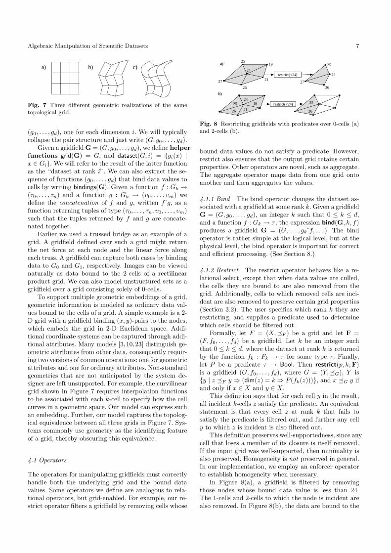
Fig. 8 Restricting gridfields with predicates over 0-cells (a)and 2-cells (b).
bound data values do not satisfy a predicate. However,restrict also ensures that the output grid retains certainproperties. Other operators are novel, such as aggregate.The aggregate operator maps data from one grid ontoanother and then aggregates the values.
4.1.1 Bind The bind operator changes the dataset as-sociated with a gridfield at some rank k. Given a gridfieldG = (G, g0, . . . , gd), an integer k such that 0 ≤ k ≤ d,and a function f : Gk → τ , the expression bind(G, k, f)produces a gridfield G = (G, . . . , gk f, . . . ). The bindoperator is rather simple at the logical level, but at thephysical level, the bind operator is important for correctand efficient processing. (See Section 8.)
4.1.2 Restrict The restrict operator behaves like a re-lational select, except that when data values are culled,the cells they are bound to are also removed from thegrid. Additionally, cells to which removed cells are inci-dent are also removed to preserve certain grid properties(Section 3.2). The user specifies which rank k they arerestricting, and supplies a predicate used to determinewhich cells should be filtered out.
Formally, let F = (X,�F ) be a grid and let F =(F, f0, . . . , fd) be a gridfield. Let k be an integer suchthat 0 ≤ k ≤ d, where the dataset at rank k is returnedby the function fk : Fk → τ for some type τ . Finally,let P be a predicate τ → Bool. Then restrict(p, k,F)is a gridfield (G, f0, . . . , fd), where G = (Y,�G), Y is{y | z �F y ⇒ (dim(z) = k ⇒ P (fk(z)))}, and x �G y ifand only if x ∈ X and y ∈ X.
This definition says that for each cell y in the result,all incident k-cells z satisfy the predicate. An equivalentstatement is that every cell z at rank k that fails tosatisfy the predicate is filtered out, and further any celly to which z is incident is also filtered out.
This definition preserves well-supportedness, since anycell that loses a member of its closure is itself removed.If the input grid was well-supported, then minimality isalso preserved. Homogeneity is not preserved in general.In our implementation, we employ an enforcer operatorto establish homogeneity when necessary.
In Figure 8(a), a gridfield is filtered by removingthose nodes whose bound data value is less than 24.The 1-cells and 2-cells to which the node is incident arealso removed. In Figure 8(b), the data are bound to the
8 Bill Howe, David Maier
2-cells; only those 2-cells whose data value fails to sat-isfy the predicate need be removed; incident 0-cells and1-cells remain.
4.1.3 Merge The merge operator computes the inter-section of two grids and retains data values defined overthis intersection. Let E = (E, e0, . . . , ec) and F = (F, f0, . . . , fd)be gridfields. Let x = min(c, d). Then merge(F,G) pro-duces a gridfield H = (F ∩ G, h0, . . . , hx) where hi =fi gi.
4.1.4 Cross Product The cross product operator for grid-fields builds on the cross product operator on grids. LetE = (E, e0, . . . , ec) and F = (F, f0, . . . , fd) be gridfields.The cross product of E and F, written E⊗F, is a grid-field G = (E ⊗ F, g0, . . . , gc+d) where gk =
∧ki=0 ei fk−i
and∧
concatenates a set of functions.This definition can result in a gridfield with values
undefined at various ranks if there are multiple ways toform cells of intermediate dimension. Consider gridfieldsE and F with the following types at each rank.
E0 : (a) F0 : (w, x)E1 : (b, c) F1 : (z)
The cross product gridfield G = E⊗F will have thefollowing types at each rank.
G0 : (a,w, x)G1 : (a, z, b, c, w, x)G2 : (b, c, w, x)
The 1-cells in the result are generated by both E0×F1
and F0 × E1. Each of these sets of cells alone wouldhave data of different types; namely, (a, z) and (b, c, w, x)respectively. However, since all cells at a particular rankmust have the same type in our model, we adopt a kindof “union” type: (a, z, b, c, w, x). Since some cells will nothave a value for a or z, we declare these values to be⊥. Therefore, all tuples at rank 1 in the result gridfieldG will be of the form (a, z,⊥,⊥,⊥,⊥) or of the form(⊥,⊥, b, c, w, x).
In the relational algebra, an analogous issue is therequirement that relations be “union-compatible” beforetheir union can be computed. The analogous solution isto coerce them to the same type, performing a kind of“outer union,” by padding the tuples with NULL andenforcing union compatibility.
4.1.5 Aggregate. The aggregate operator maps a sourcegridfield’s cells onto a target gridfield’s cells, and then ag-gregates the data values bound to the mapped cells. Thebehavior of aggregate is controlled by two functions, anassignment function and an aggregation function. Theassignment function associates each cell in the targetgrid with a set of cells in the source grid. To perform
12.1°C12.6°C 13.1°C 13.2°C 12.8°C 12.5°C
{12.6°C, 13.1°C, 13.2°C}
{12.8°C , 12.5°C , 12.1°C}
12.95°C 12.45°C
a)
Assignment
Aggregation
b)
c)
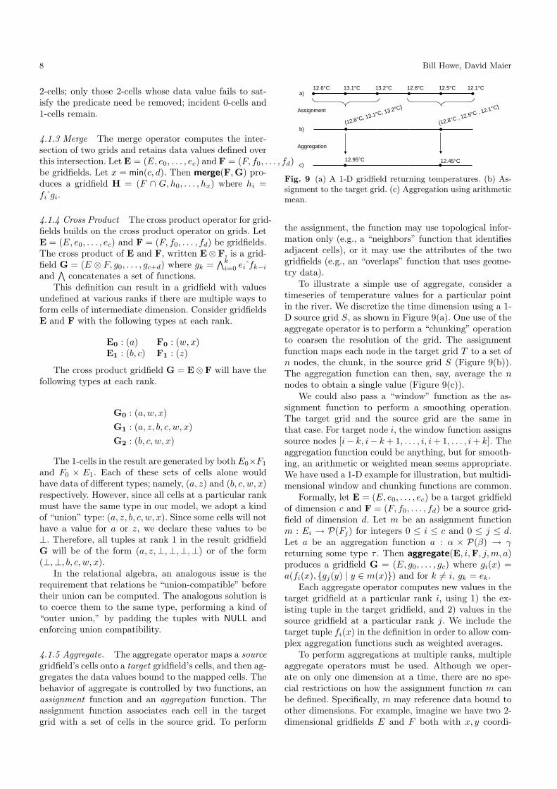
Fig. 9 (a) A 1-D gridfield returning temperatures. (b) As-signment to the target grid. (c) Aggregation using arithmeticmean.
the assignment, the function may use topological infor-mation only (e.g., a “neighbors” function that identifiesadjacent cells), or it may use the attributes of the twogridfields (e.g., an “overlaps” function that uses geome-try data).
To illustrate a simple use of aggregate, consider atimeseries of temperature values for a particular pointin the river. We discretize the time dimension using a 1-D source grid S, as shown in Figure 9(a). One use of theaggregate operator is to perform a “chunking” operationto coarsen the resolution of the grid. The assignmentfunction maps each node in the target grid T to a set ofn nodes, the chunk, in the source grid S (Figure 9(b)).The aggregation function can then, say, average the nnodes to obtain a single value (Figure 9(c)).
We could also pass a “window” function as the as-signment function to perform a smoothing operation.The target grid and the source grid are the same inthat case. For target node i, the window function assignssource nodes [i− k, i− k + 1, . . . , i, i + 1, . . . , i + k]. Theaggregation function could be anything, but for smooth-ing, an arithmetic or weighted mean seems appropriate.We have used a 1-D example for illustration, but multidi-mensional window and chunking functions are common.
Formally, let E = (E, e0, . . . , ec) be a target gridfieldof dimension c and F = (F, f0, . . . , fd) be a source grid-field of dimension d. Let m be an assignment functionm : Ei → P(Fj) for integers 0 ≤ i ≤ c and 0 ≤ j ≤ d.Let a be an aggregation function a : α × P(β) → γreturning some type τ . Then aggregate(E, i,F, j,m, a)produces a gridfield G = (E, g0, . . . , gc) where gi(x) =a(fi(x), {gj(y) | y ∈ m(x)}) and for k 6= i, gk = ek.
Each aggregate operator computes new values in thetarget gridfield at a particular rank i, using 1) the ex-isting tuple in the target gridfield, and 2) values in thesource gridfield at a particular rank j. We include thetarget tuple fi(x) in the definition in order to allow com-plex aggregation functions such as weighted averages.
To perform aggregations at multiple ranks, multipleaggregate operators must be used. Although we oper-ate on only one dimension at a time, there are no spe-cial restrictions on how the assignment function m canbe defined. Specifically, m may reference data bound toother dimensions. For example, imagine we have two 2-dimensional gridfields E and F both with x, y coordi-
Algebraic Manipulation of Scientific Datasets 9
nates bound to their nodes. Further, the source grid Fhas a temperature dataset bound to its 2-cells. A com-mon aggregation is to “regrid” the temperature datasetby averaging the values of 2-cells that overlap a giventarget 2-cell [11]. In this case, i = j = 2. However, thegeometry data of both grids must be accessed to evalu-ate the “overlaps” predicate. Specifically, the assignmentfunction returns the set of polygons in F that overlap agiven polygon in E. Intuitively, the aggregate operatormimics the functionality of a (possibly spatial) join fol-lowed by a group by in the relational algebra.
A precise model of the information that an assign-ment function consume during evaluation can lead tomore efficient implementations. An assignment functionthat consumes only bound data values (like a standardrelational join predicate) need not have access to the in-cidence relation, which might allow an evaluation engineto ignore the grid altogether. Conversely, an assignmentfunction based solely on topology can be pre-computedbefore bound data becomes available. For example, asmoothing operation that averages the values of neigh-boring cells can be defined using an instance of the ag-gregate operator. If the same grid is reused with newdatasets produced daily, neighborhood information canbe precomputed and cached. This optimization wouldbe reflected in equivalence laws in the physical gridfieldalgebra only, as the logical model prescribes one oper-ator for both assignment and aggregation. We discussevaluation techniques in more detail in Section 7.
4.1.6 Aggregate Specializations. The aggregate opera-tor is very expressive, and is quite common in recipes.For frequently occurring cases, we have defined special-izations both for syntactic convenience and to allow moreefficient implementations. For example, the project op-erator assumes identical source and target gridfields anduses a trivial assignment function that maps each cell toitself (the identity function). The aggregation functionsimply removes user-specified attributes from each log-ical tuple at a specified rank. The apply operator usesthe same trivial assignment function, but accepts a user-defined arithmetic expression and evaluates it for eachtuple at a specified rank. For a more efficient implemen-tation, we can “compile” the expression prior to the firstevaluation. The unify operator aggregates all of the val-ues in a grid to a single value. The target grid of the unifyoperator is the unit grid consisting of a single node andno higher-dimensional cells. The unit grid is the identityof the cross product operator, up to isomorphism. Theassignment function used in the unify operator maps ev-ery cell in the source grid to the single node in the unitgrid; the user supplies an integer rank and an arbitraryaggregation function.
4.2 Features
We summarize the features of our data model:
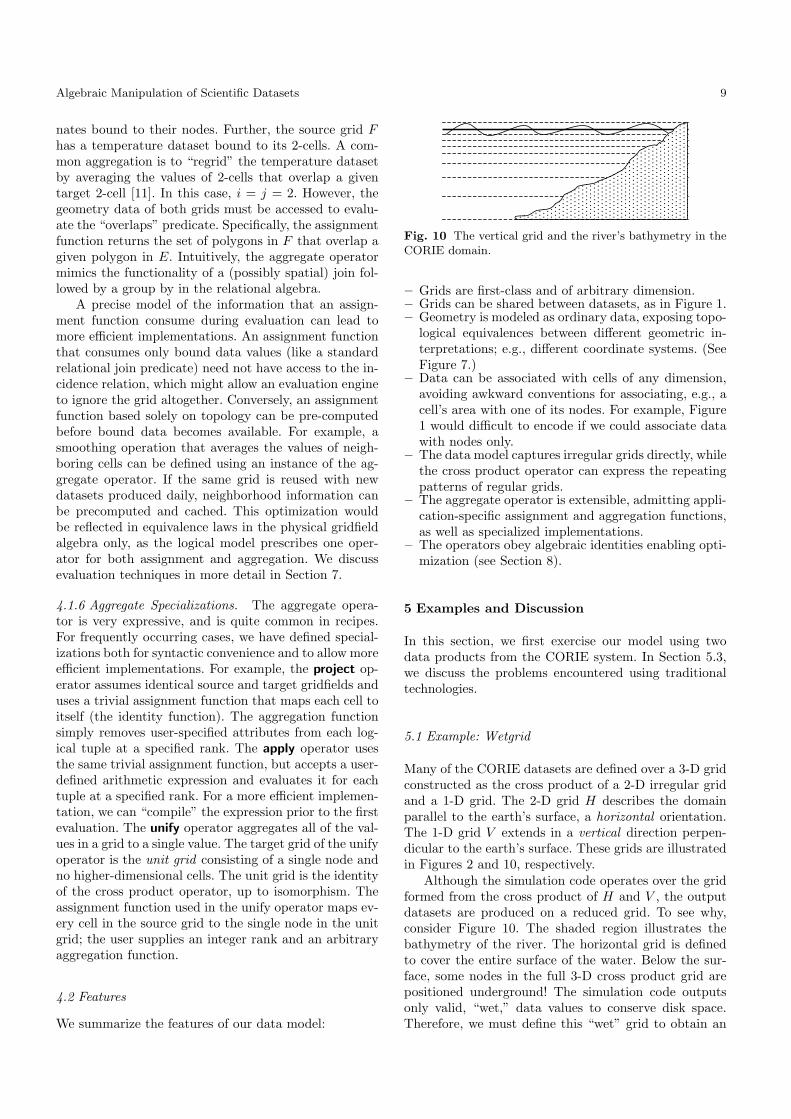
Fig. 10 The vertical grid and the river’s bathymetry in theCORIE domain.
– Grids are first-class and of arbitrary dimension.– Grids can be shared between datasets, as in Figure 1.– Geometry is modeled as ordinary data, exposing topo-
logical equivalences between different geometric in-terpretations; e.g., different coordinate systems. (SeeFigure 7.)
– Data can be associated with cells of any dimension,avoiding awkward conventions for associating, e.g., acell’s area with one of its nodes. For example, Figure1 would difficult to encode if we could associate datawith nodes only.
– The data model captures irregular grids directly, whilethe cross product operator can express the repeatingpatterns of regular grids.
– The aggregate operator is extensible, admitting appli-cation-specific assignment and aggregation functions,as well as specialized implementations.
– The operators obey algebraic identities enabling opti-mization (see Section 8).
5 Examples and Discussion
In this section, we first exercise our model using twodata products from the CORIE system. In Section 5.3,we discuss the problems encountered using traditionaltechnologies.
5.1 Example: Wetgrid
Many of the CORIE datasets are defined over a 3-D gridconstructed as the cross product of a 2-D irregular gridand a 1-D grid. The 2-D grid H describes the domainparallel to the earth’s surface, a horizontal orientation.The 1-D grid V extends in a vertical direction perpen-dicular to the earth’s surface. These grids are illustratedin Figures 2 and 10, respectively.
Although the simulation code operates over the gridformed from the cross product of H and V , the outputdatasets are produced on a reduced grid. To see why,consider Figure 10. The shaded region illustrates thebathymetry of the river. The horizontal grid is definedto cover the entire surface of the water. Below the sur-face, some nodes in the full 3-D cross product grid arepositioned underground! The simulation code outputsonly valid, “wet,” data values to conserve disk space.Therefore, we must define this “wet” grid to obtain an
10 Bill Howe, David Maier
⊗
H0 : (x,y,b)
V0 : (z)
render
“wetgrid” O0 : (x,y,z,b,salt)
restrict(0, z >b) bind(0,salt) restrict(0, ocean)
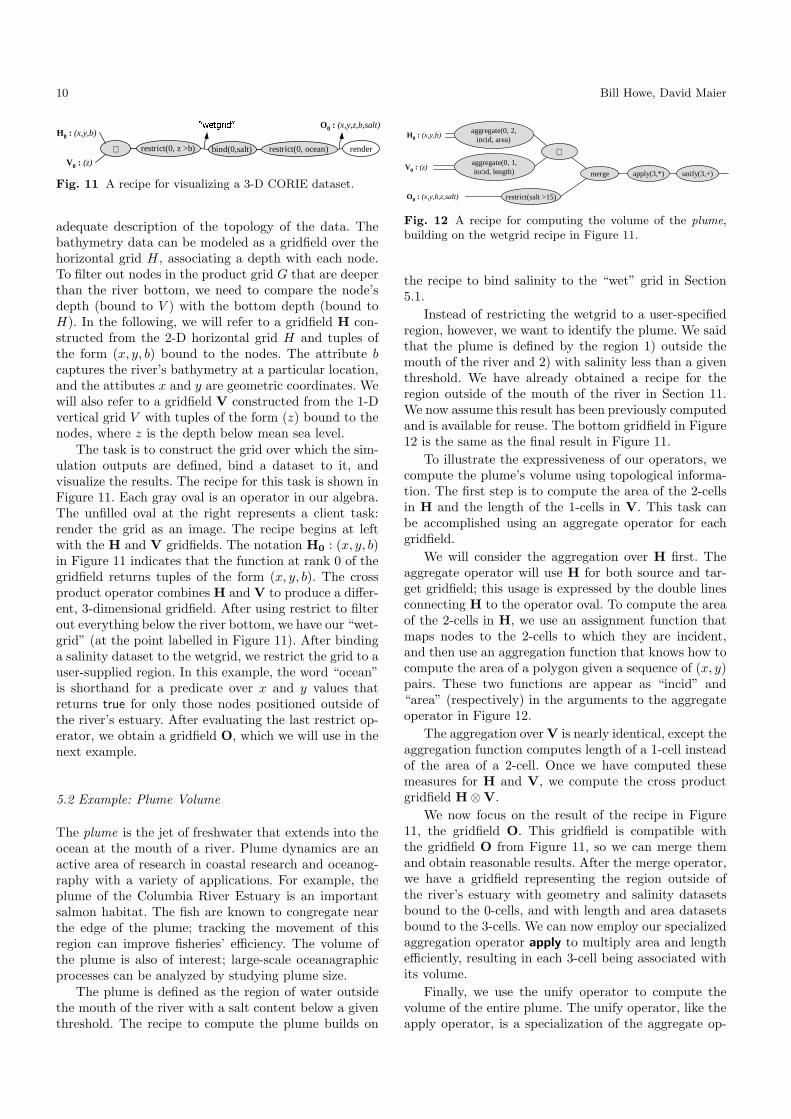
Fig. 11 A recipe for visualizing a 3-D CORIE dataset.
adequate description of the topology of the data. Thebathymetry data can be modeled as a gridfield over thehorizontal grid H, associating a depth with each node.To filter out nodes in the product grid G that are deeperthan the river bottom, we need to compare the node’sdepth (bound to V ) with the bottom depth (bound toH). In the following, we will refer to a gridfield H con-structed from the 2-D horizontal grid H and tuples ofthe form (x, y, b) bound to the nodes. The attribute bcaptures the river’s bathymetry at a particular location,and the attibutes x and y are geometric coordinates. Wewill also refer to a gridfield V constructed from the 1-Dvertical grid V with tuples of the form (z) bound to thenodes, where z is the depth below mean sea level.
The task is to construct the grid over which the sim-ulation outputs are defined, bind a dataset to it, andvisualize the results. The recipe for this task is shown inFigure 11. Each gray oval is an operator in our algebra.The unfilled oval at the right represents a client task:render the grid as an image. The recipe begins at leftwith the H and V gridfields. The notation H0 : (x, y, b)in Figure 11 indicates that the function at rank 0 of thegridfield returns tuples of the form (x, y, b). The crossproduct operator combines H and V to produce a differ-ent, 3-dimensional gridfield. After using restrict to filterout everything below the river bottom, we have our “wet-grid” (at the point labelled in Figure 11). After bindinga salinity dataset to the wetgrid, we restrict the grid to auser-supplied region. In this example, the word “ocean”is shorthand for a predicate over x and y values thatreturns true for only those nodes positioned outside ofthe river’s estuary. After evaluating the last restrict op-erator, we obtain a gridfield O, which we will use in thenext example.
5.2 Example: Plume Volume
The plume is the jet of freshwater that extends into theocean at the mouth of a river. Plume dynamics are anactive area of research in coastal research and oceanog-raphy with a variety of applications. For example, theplume of the Columbia River Estuary is an importantsalmon habitat. The fish are known to congregate nearthe edge of the plume; tracking the movement of thisregion can improve fisheries’ efficiency. The volume ofthe plume is also of interest; large-scale oceanagraphicprocesses can be analyzed by studying plume size.
The plume is defined as the region of water outsidethe mouth of the river with a salt content below a giventhreshold. The recipe to compute the plume builds on
⊗
H0 : (x,y,b)
V0 : (z)merge
aggregate(0, 2,incid, area)
unify(3,+)
O0 : (x,y,b,z,salt)
apply(3,*)
restrict(salt >15)
aggregate(0, 1,incid, length)
Fig. 12 A recipe for computing the volume of the plume,building on the wetgrid recipe in Figure 11.
the recipe to bind salinity to the “wet” grid in Section5.1.
Instead of restricting the wetgrid to a user-specifiedregion, however, we want to identify the plume. We saidthat the plume is defined by the region 1) outside themouth of the river and 2) with salinity less than a giventhreshold. We have already obtained a recipe for theregion outside of the mouth of the river in Section 11.We now assume this result has been previously computedand is available for reuse. The bottom gridfield in Figure12 is the same as the final result in Figure 11.
To illustrate the expressiveness of our operators, wecompute the plume’s volume using topological informa-tion. The first step is to compute the area of the 2-cellsin H and the length of the 1-cells in V. This task canbe accomplished using an aggregate operator for eachgridfield.
We will consider the aggregation over H first. Theaggregate operator will use H for both source and tar-get gridfield; this usage is expressed by the double linesconnecting H to the operator oval. To compute the areaof the 2-cells in H, we use an assignment function thatmaps nodes to the 2-cells to which they are incident,and then use an aggregation function that knows how tocompute the area of a polygon given a sequence of (x, y)pairs. These two functions are appear as “incid” and“area” (respectively) in the arguments to the aggregateoperator in Figure 12.
The aggregation over V is nearly identical, except theaggregation function computes length of a 1-cell insteadof the area of a 2-cell. Once we have computed thesemeasures for H and V, we compute the cross productgridfield H⊗V.
We now focus on the result of the recipe in Figure11, the gridfield O. This gridfield is compatible withthe gridfield O from Figure 11, so we can merge themand obtain reasonable results. After the merge operator,we have a gridfield representing the region outside ofthe river’s estuary with geometry and salinity datasetsbound to the 0-cells, and with length and area datasetsbound to the 3-cells. We can now employ our specializedaggregation operator apply to multiply area and lengthefficiently, resulting in each 3-cell being associated withits volume.
Finally, we use the unify operator to compute thevolume of the entire plume. The unify operator, like theapply operator, is a specialization of the aggregate op-
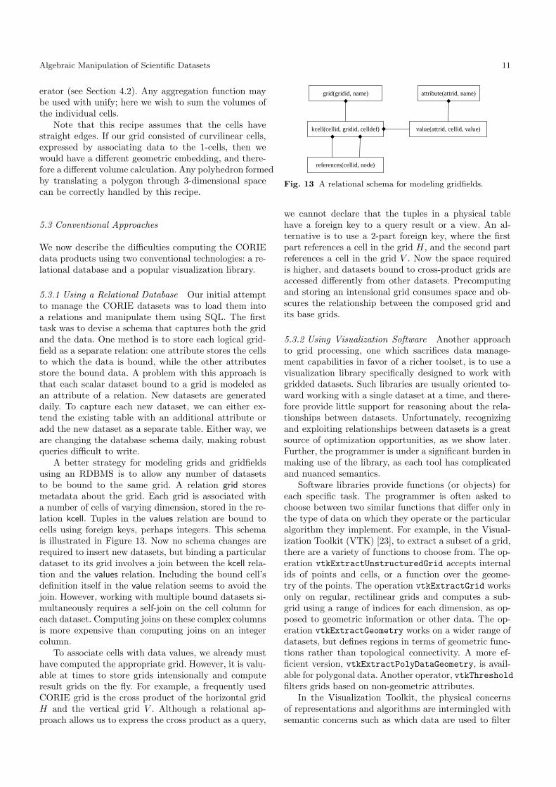
Algebraic Manipulation of Scientific Datasets 11
erator (see Section 4.2). Any aggregation function maybe used with unify; here we wish to sum the volumes ofthe individual cells.
Note that this recipe assumes that the cells havestraight edges. If our grid consisted of curvilinear cells,expressed by associating data to the 1-cells, then wewould have a different geometric embedding, and there-fore a different volume calculation. Any polyhedron formedby translating a polygon through 3-dimensional spacecan be correctly handled by this recipe.
5.3 Conventional Approaches
We now describe the difficulties computing the CORIEdata products using two conventional technologies: a re-lational database and a popular visualization library.
5.3.1 Using a Relational Database Our initial attemptto manage the CORIE datasets was to load them intoa relations and manipulate them using SQL. The firsttask was to devise a schema that captures both the gridand the data. One method is to store each logical grid-field as a separate relation: one attribute stores the cellsto which the data is bound, while the other attributesstore the bound data. A problem with this approach isthat each scalar dataset bound to a grid is modeled asan attribute of a relation. New datasets are generateddaily. To capture each new dataset, we can either ex-tend the existing table with an additional attribute oradd the new dataset as a separate table. Either way, weare changing the database schema daily, making robustqueries difficult to write.
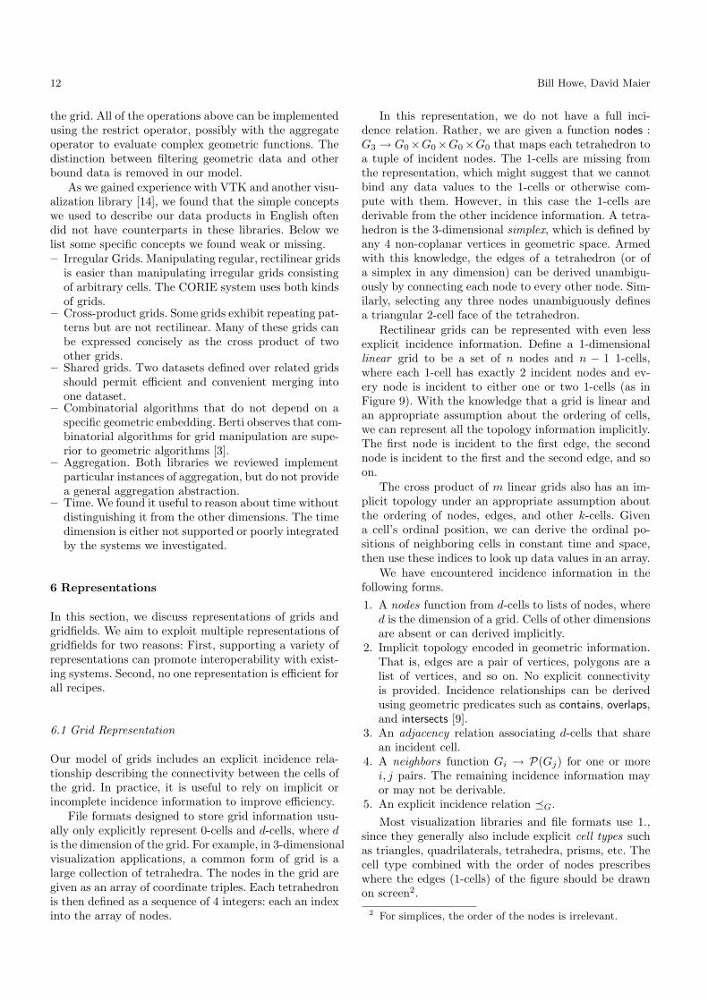
A better strategy for modeling grids and gridfieldsusing an RDBMS is to allow any number of datasetsto be bound to the same grid. A relation grid storesmetadata about the grid. Each grid is associated witha number of cells of varying dimension, stored in the re-lation kcell. Tuples in the values relation are bound tocells using foreign keys, perhaps integers. This schemais illustrated in Figure 13. Now no schema changes arerequired to insert new datasets, but binding a particulardataset to its grid involves a join between the kcell rela-tion and the values relation. Including the bound cell’sdefinition itself in the value relation seems to avoid thejoin. However, working with multiple bound datasets si-multaneously requires a self-join on the cell column foreach dataset. Computing joins on these complex columnsis more expensive than computing joins on an integercolumn.
To associate cells with data values, we already musthave computed the appropriate grid. However, it is valu-able at times to store grids intensionally and computeresult grids on the fly. For example, a frequently usedCORIE grid is the cross product of the horizontal gridH and the vertical grid V . Although a relational ap-proach allows us to express the cross product as a query,
grid(gridid, name)
kcell(cellid, gridid, celldef)
attribute(attrid, name)
value(attrid, cellid, value)
references(cellid, node)
Fig. 13 A relational schema for modeling gridfields.
we cannot declare that the tuples in a physical tablehave a foreign key to a query result or a view. An al-ternative is to use a 2-part foreign key, where the firstpart references a cell in the grid H, and the second partreferences a cell in the grid V . Now the space requiredis higher, and datasets bound to cross-product grids areaccessed differently from other datasets. Precomputingand storing an intensional grid consumes space and ob-scures the relationship between the composed grid andits base grids.
5.3.2 Using Visualization Software Another approachto grid processing, one which sacrifices data manage-ment capabilities in favor of a richer toolset, is to use avisualization library specifically designed to work withgridded datasets. Such libraries are usually oriented to-ward working with a single dataset at a time, and there-fore provide little support for reasoning about the rela-tionships between datasets. Unfortunately, recognizingand exploiting relationships between datasets is a greatsource of optimization opportunities, as we show later.Further, the programmer is under a significant burden inmaking use of the library, as each tool has complicatedand nuanced semantics.
Software libraries provide functions (or objects) foreach specific task. The programmer is often asked tochoose between two similar functions that differ only inthe type of data on which they operate or the particularalgorithm they implement. For example, in the Visual-ization Toolkit (VTK) [23], to extract a subset of a grid,there are a variety of functions to choose from. The op-eration vtkExtractUnstructuredGrid accepts internalids of points and cells, or a function over the geome-try of the points. The operation vtkExtractGrid worksonly on regular, rectilinear grids and computes a sub-grid using a range of indices for each dimension, as op-posed to geometric information or other data. The op-eration vtkExtractGeometry works on a wider range ofdatasets, but defines regions in terms of geometric func-tions rather than topological connectivity. A more ef-ficient version, vtkExtractPolyDataGeometry, is avail-able for polygonal data. Another operator, vtkThresholdfilters grids based on non-geometric attributes.
In the Visualization Toolkit, the physical concernsof representations and algorithms are intermingled withsemantic concerns such as which data are used to filter
12 Bill Howe, David Maier
the grid. All of the operations above can be implementedusing the restrict operator, possibly with the aggregateoperator to evaluate complex geometric functions. Thedistinction between filtering geometric data and otherbound data is removed in our model.
As we gained experience with VTK and another visu-alization library [14], we found that the simple conceptswe used to describe our data products in English oftendid not have counterparts in these libraries. Below welist some specific concepts we found weak or missing.– Irregular Grids. Manipulating regular, rectilinear grids
is easier than manipulating irregular grids consistingof arbitrary cells. The CORIE system uses both kindsof grids.
– Cross-product grids. Some grids exhibit repeating pat-terns but are not rectilinear. Many of these grids canbe expressed concisely as the cross product of twoother grids.
– Shared grids. Two datasets defined over related gridsshould permit efficient and convenient merging intoone dataset.
– Combinatorial algorithms that do not depend on aspecific geometric embedding. Berti observes that com-binatorial algorithms for grid manipulation are supe-rior to geometric algorithms [3].
– Aggregation. Both libraries we reviewed implementparticular instances of aggregation, but do not providea general aggregation abstraction.
– Time. We found it useful to reason about time withoutdistinguishing it from the other dimensions. The timedimension is either not supported or poorly integratedby the systems we investigated.
6 Representations
In this section, we discuss representations of grids andgridfields. We aim to exploit multiple representations ofgridfields for two reasons: First, supporting a variety ofrepresentations can promote interoperability with exist-ing systems. Second, no one representation is efficient forall recipes.
6.1 Grid Representation
Our model of grids includes an explicit incidence rela-tionship describing the connectivity between the cells ofthe grid. In practice, it is useful to rely on implicit orincomplete incidence information to improve efficiency.
File formats designed to store grid information usu-ally only explicitly represent 0-cells and d-cells, where dis the dimension of the grid. For example, in 3-dimensionalvisualization applications, a common form of grid is alarge collection of tetrahedra. The nodes in the grid aregiven as an array of coordinate triples. Each tetrahedronis then defined as a sequence of 4 integers: each an indexinto the array of nodes.
In this representation, we do not have a full inci-dence relation. Rather, we are given a function nodes :G3 → G0×G0×G0×G0 that maps each tetrahedron toa tuple of incident nodes. The 1-cells are missing fromthe representation, which might suggest that we cannotbind any data values to the 1-cells or otherwise com-pute with them. However, in this case the 1-cells arederivable from the other incidence information. A tetra-hedron is the 3-dimensional simplex, which is defined byany 4 non-coplanar vertices in geometric space. Armedwith this knowledge, the edges of a tetrahedron (or ofa simplex in any dimension) can be derived unambigu-ously by connecting each node to every other node. Sim-ilarly, selecting any three nodes unambiguously definesa triangular 2-cell face of the tetrahedron.
Rectilinear grids can be represented with even lessexplicit incidence information. Define a 1-dimensionallinear grid to be a set of n nodes and n − 1 1-cells,where each 1-cell has exactly 2 incident nodes and ev-ery node is incident to either one or two 1-cells (as inFigure 9). With the knowledge that a grid is linear andan appropriate assumption about the ordering of cells,we can represent all the topology information implicitly.The first node is incident to the first edge, the secondnode is incident to the first and the second edge, and soon.
The cross product of m linear grids also has an im-plicit topology under an appropriate assumption aboutthe ordering of nodes, edges, and other k-cells. Givena cell’s ordinal position, we can derive the ordinal po-sitions of neighboring cells in constant time and space,then use these indices to look up data values in an array.
We have encountered incidence information in thefollowing forms.1. A nodes function from d-cells to lists of nodes, where
d is the dimension of a grid. Cells of other dimensionsare absent or can derived implicitly.
2. Implicit topology encoded in geometric information.That is, edges are a pair of vertices, polygons are alist of vertices, and so on. No explicit connectivityis provided. Incidence relationships can be derivedusing geometric predicates such as contains, overlaps,and intersects [9].
3. An adjacency relation associating d-cells that sharean incident cell.
4. A neighbors function Gi → P(Gj) for one or morei, j pairs. The remaining incidence information mayor may not be derivable.
5. An explicit incidence relation �G.Most visualization libraries and file formats use 1.,
since they generally also include explicit cell types suchas triangles, quadrilaterals, tetrahedra, prisms, etc. Thecell type combined with the order of nodes prescribeswhere the edges (1-cells) of the figure should be drawnon screen2.
2 For simplices, the order of the nodes is irrelevant.
Algebraic Manipulation of Scientific Datasets 13
Most GIS and spatial database systems use 2., re-lying on geometric functions to determine topologicalrelationships [9]. To determine which cells are adjacentto a given cell, users write a query over a relation witha geometric attribute containing points, lines, polylines,polygons, and so on.
In our representation (described in Section 6.2), eachcell of dimension greater than zero contains as an ar-ray of nodes, providing a function nodes : Gk → P(G0)for all 0 ≤ k ≤ d. Additionally, we use a hash indexto implement a function cells : G0 → P(Gk) mappingnodes to the cells to which they are incident. To de-rive incidence information between arbitrary i-cells andj-cells, we assume that a cell x is incident to a cell y ifnodes(x) ⊆ nodes(y). This representation corresponds to4. on our list.
Without complete incidence information (implicit orexplicit), some generality of the data model is lost. Forexample, visualization systems do not allow data to bebound to the edges of a 2-d grid. However, for manyapplications this feature is unnecessary, and carryingaround explicit incidence information for an unneededfeature can be expensive. As an evaluation technique,an optimizer might determine that 1-cells are not ac-cessed in a particular recipe and therefore prune themfrom intermediate results. We exploit this optimizationto improve performance of the cross product operator inSection 8.
6.2 Gridfield Representations
The data bound to a grid also offers several choices ofrepresentation. We have identified four major patternsof gridfield representation used in practice.
The tabular representation forms 〈cell, value〉 tuples,making it easy to pipeline data from one operator toanother, but difficult to separate grid from data.
The parallel representation uses a separate array foreach attribute, all aligned positionally with another ar-ray for the cells to which the attributes are bound. Withthis representation, binding in new attributes and pro-jecting out unneeded ones are trivial operations.
The decomposed representation stores an intensionaldescription of the desired gridfield rather than an ex-plicit representation of it. A decomposed representationof cross-product gridfields is especially useful, since thethe two factors of a product gridfield require less storagespace than the result.
The nested representation involves gridfield attributesthat can themselves be gridfields. A 4-D time-space grid-field may be a timeseries (the outer grid) and a 3-D spa-tial grid (the inner, nested grid).
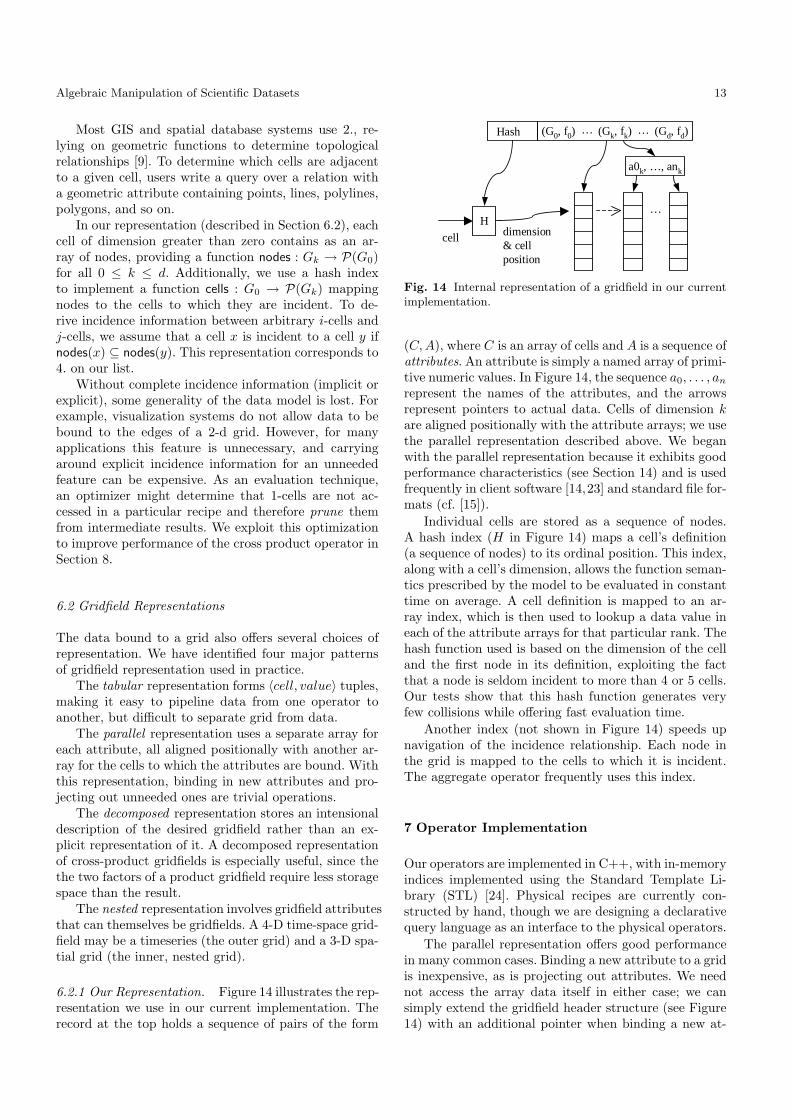
6.2.1 Our Representation. Figure 14 illustrates the rep-resentation we use in our current implementation. Therecord at the top holds a sequence of pairs of the form
…
Hdimension& cell position
cell
Hash (Gd, fd)
a0k, …, ank
…
(G0, f0) … (Gk, fk)
Fig. 14 Internal representation of a gridfield in our currentimplementation.
(C,A), where C is an array of cells and A is a sequence ofattributes. An attribute is simply a named array of primi-tive numeric values. In Figure 14, the sequence a0, . . . , an
represent the names of the attributes, and the arrowsrepresent pointers to actual data. Cells of dimension kare aligned positionally with the attribute arrays; we usethe parallel representation described above. We beganwith the parallel representation because it exhibits goodperformance characteristics (see Section 14) and is usedfrequently in client software [14,23] and standard file for-mats (cf. [15]).
Individual cells are stored as a sequence of nodes.A hash index (H in Figure 14) maps a cell’s definition(a sequence of nodes) to its ordinal position. This index,along with a cell’s dimension, allows the function seman-tics prescribed by the model to be evaluated in constanttime on average. A cell definition is mapped to an ar-ray index, which is then used to lookup a data value ineach of the attribute arrays for that particular rank. Thehash function used is based on the dimension of the celland the first node in its definition, exploiting the factthat a node is seldom incident to more than 4 or 5 cells.Our tests show that this hash function generates veryfew collisions while offering fast evaluation time.
Another index (not shown in Figure 14) speeds upnavigation of the incidence relationship. Each node inthe grid is mapped to the cells to which it is incident.The aggregate operator frequently uses this index.
7 Operator Implementation
Our operators are implemented in C++, with in-memoryindices implemented using the Standard Template Li-brary (STL) [24]. Physical recipes are currently con-structed by hand, though we are designing a declarativequery language as an interface to the physical operators.
The parallel representation offers good performancein many common cases. Binding a new attribute to a gridis inexpensive, as is projecting out attributes. We neednot access the array data itself in either case; we cansimply extend the gridfield header structure (see Figure14) with an additional pointer when binding a new at-

14 Bill Howe, David Maier
tribute, or just remove a pointer when an attribute isprojected away.
The merge operator computes the intersection of twogrids during evaluation, and is therefore potentially ex-pensive. However, if the two argument gridfields are de-fined over the same grid, the intersection is trivial tocompute, and merge can be evaluated in constant time.Since gridfields may share grids via pointers, checkingfor grid equivalence in this case is essentially free.
The aggregate operator accepts function objects de-fined as classes in C++, and evaluates them in the man-ner implied directly by the model. Each assignment func-tion may potentially access data values as well as topol-ogy information, so no guarantees can be made about itstime complexity. Each aggregation function can be pa-rameterized by names of attributes or other user-suppliedinformation. Provided all required parameters and thetype of its input, the aggregation function must announcethe type of its output. For example, a sum function mightbe parameterized by the name of an attribute “a” andoutput a tuple with just a single attribute “sum a” re-gardless of input. An alternative version of sum mightnot take any parameters, but produce an attribute “sum x”for each numeric attribute x in the input type.
This implementation of the aggregate operator is fullygeneralized, but can be somewhat inefficient. For eachcell in the target grid, we must 1) evaluate a potentiallyexpensive assignment function to produce a set of cells,2) probe the hash index of the source grid for each ofthese cells, 3) construct a set of tuples from the resultsof the hash index, and 4) evaluate a potentially expen-sive aggregation function for the set of tuples. We arecurrently working on categorizing assignment functionsbased on the information they require (topology only,topology and data values, data values only). Each cate-gory of assignment function will give rise to a specializedimplementation of the aggregate operator exhibiting im-proved performance.
Other grid relationships can also be exploited duringevaluation of a merge operator. At the logical level, twogridfields G and F can be merged in constant time if weknow that grid(G) ⊂ grid(F). The domain of the func-tions fi ∈ bindings(G) is simply reduced. At the physicallevel, we do not have true functions, but rather explicitarrays. Therefore, the array representing the range of fmust be filtered to remove values associated with cellsnot in G. This step requires linear time using the hashindex H to map cells to their ordinal positions.
Cross product is usually the most expensive opera-tor in the algebra. In the next section, we investigatealgebraic rewrites to reduce its cost or remove it alto-gether. We can also improve its implementation in somecases. The cross product of a grid with nodes, edges,and polygons and a grid with nodes and edges producesnodes, edges, polygons, and polyhedra. However, for vi-sualization purposes, we may only need the polyhedraand the nodes; cells of intermediate dimensions need not
⊗
H0 : (x,y,b)
V0 : (z)
render
restrict(ocean)
restrict(z>b) bind(salt)
Fig. 15 An optimized recipe for visualizing a 3-D CORIEdataset.
be computed. However, to use such a “pruning” imple-mentation, we must be able to determine which dimen-sion cells will be consumed downstream in a recipe.
Another implementation of the cross product oper-ator (applicable to Figure 11) exploits the fact that itis followed immediately by a restrict. In relational alge-bra, a join is semantically equivalent to a cross productfollowed by a select. We can create an analogous “join”operator that evaluates the restrict as the cross productis computed, creating fewer cells overall.
8 Optimization
Having described our data representation and operatorimplementation, we now present optimization techniquesenabled by our algebra for improving the performance ofrecipes. Our examples are actual CORIE data products,though the techniques we use generalize to any domaininvolving irregular grids, cross product grids, or selectedsub-regions.
8.1 Commuting Restrictions.
The recipe in Figure 11 computes a 3-D salinity grid-field, then restricts the result to a user-specified region.The logical model allows us to freely commute the re-strict operator with the bind, and then with the crossproduct [13], to significantly reduce the size of the in-termediate results. However, our representation materi-alizes functions as arrays. These attribute arrays mustbe positionally aligned with an array of cells so that thefirst data value corresponds to first cell, and so on. Withthis representation, it is easy to bind a new attributearray: we simply add a pointer to the gridfield headerstructure. (Specifically, we add an item to the sequencea0, . . . , an in Figure 14.) However, if we push the restrictbefore the bind, we will be binding an attribute array ofN elements to a grid with less than N 0-cells. If thisoccurs, a critical invariant of the representation will bebroken.
To solve this problem, we can pre-compute the ordi-nal positions of cells in the wetgrid and record these datain an attribute array named “positions.” The bind oper-ator can use the “positions” attribute to stride throughdata on disk and avoid those data that correspond tofiltered out cells. This technique allows the restrict op-erator to commute with bind at the physical level.
Our goal is to push the final restrict operator evenfurther, in order to reduce the work required by the cross
Algebraic Manipulation of Scientific Datasets 15
a)
b)
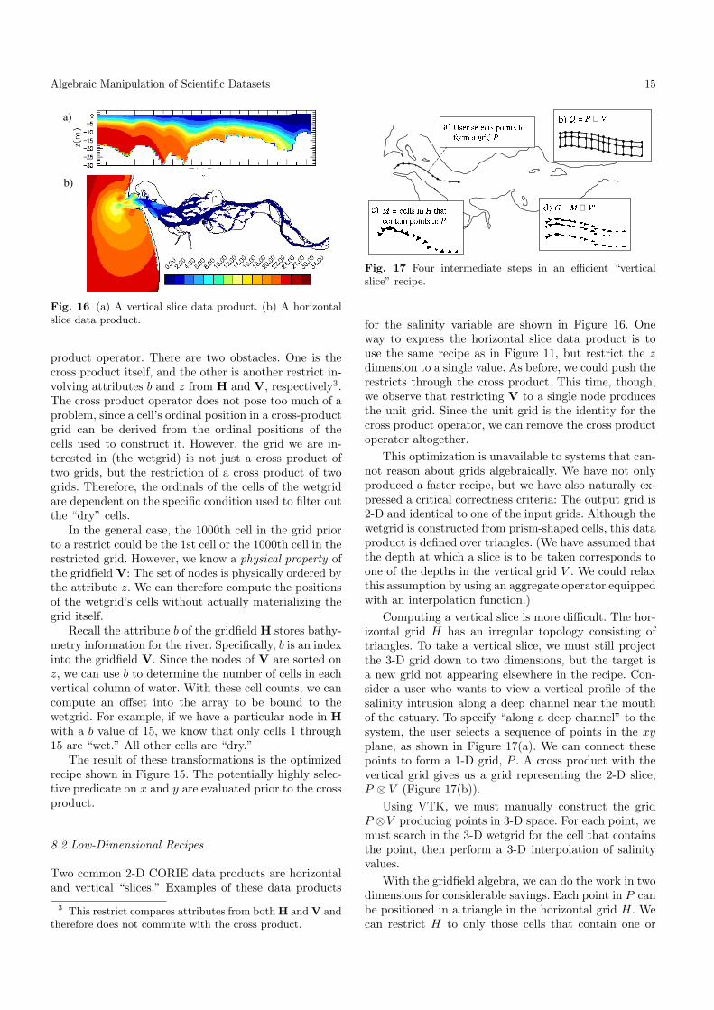
Fig. 16 (a) A vertical slice data product. (b) A horizontalslice data product.
product operator. There are two obstacles. One is thecross product itself, and the other is another restrict in-volving attributes b and z from H and V, respectively3.The cross product operator does not pose too much of aproblem, since a cell’s ordinal position in a cross-productgrid can be derived from the ordinal positions of thecells used to construct it. However, the grid we are in-terested in (the wetgrid) is not just a cross product oftwo grids, but the restriction of a cross product of twogrids. Therefore, the ordinals of the cells of the wetgridare dependent on the specific condition used to filter outthe “dry” cells.
In the general case, the 1000th cell in the grid priorto a restrict could be the 1st cell or the 1000th cell in therestricted grid. However, we know a physical property ofthe gridfield V: The set of nodes is physically ordered bythe attribute z. We can therefore compute the positionsof the wetgrid’s cells without actually materializing thegrid itself.
Recall the attribute b of the gridfield H stores bathy-metry information for the river. Specifically, b is an indexinto the gridfield V. Since the nodes of V are sorted onz, we can use b to determine the number of cells in eachvertical column of water. With these cell counts, we cancompute an offset into the array to be bound to thewetgrid. For example, if we have a particular node in Hwith a b value of 15, we know that only cells 1 through15 are “wet.” All other cells are “dry.”
The result of these transformations is the optimizedrecipe shown in Figure 15. The potentially highly selec-tive predicate on x and y are evaluated prior to the crossproduct.
8.2 Low-Dimensional Recipes
Two common 2-D CORIE data products are horizontaland vertical “slices.” Examples of these data products
3 This restrict compares attributes from both H and V andtherefore does not commute with the cross product.
���������⊗ ��� ������������������ �"!�#%$'&)( *,+.-
/1032547698�:5;=<�>
?A@CBEDGF�H�I.J�K,L.MONQP.RTSVUW�X%Y)Z1[V\']_^�`%a.b)ced,f.g_h
ikj�l�mon⊗ prq
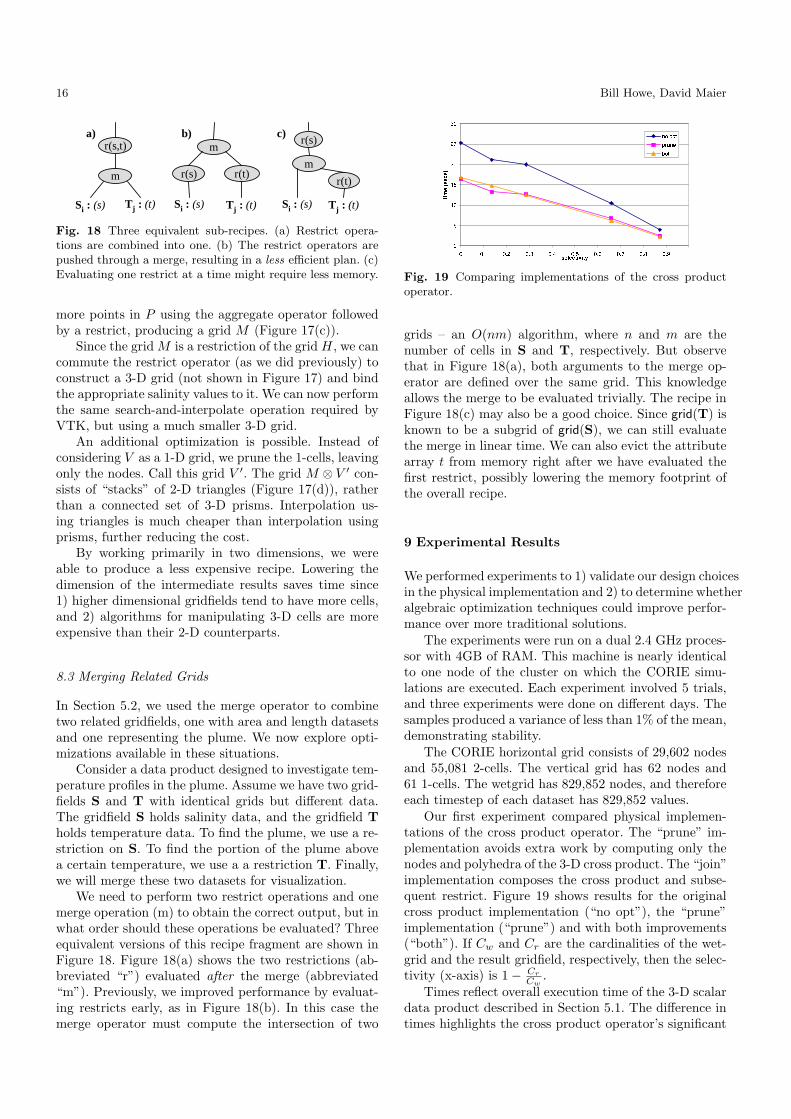
Fig. 17 Four intermediate steps in an efficient “verticalslice” recipe.
for the salinity variable are shown in Figure 16. Oneway to express the horizontal slice data product is touse the same recipe as in Figure 11, but restrict the zdimension to a single value. As before, we could push therestricts through the cross product. This time, though,we observe that restricting V to a single node producesthe unit grid. Since the unit grid is the identity for thecross product operator, we can remove the cross productoperator altogether.
This optimization is unavailable to systems that can-not reason about grids algebraically. We have not onlyproduced a faster recipe, but we have also naturally ex-pressed a critical correctness criteria: The output grid is2-D and identical to one of the input grids. Although thewetgrid is constructed from prism-shaped cells, this dataproduct is defined over triangles. (We have assumed thatthe depth at which a slice is to be taken corresponds toone of the depths in the vertical grid V . We could relaxthis assumption by using an aggregate operator equippedwith an interpolation function.)
Computing a vertical slice is more difficult. The hor-izontal grid H has an irregular topology consisting oftriangles. To take a vertical slice, we must still projectthe 3-D grid down to two dimensions, but the target isa new grid not appearing elsewhere in the recipe. Con-sider a user who wants to view a vertical profile of thesalinity intrusion along a deep channel near the mouthof the estuary. To specify “along a deep channel” to thesystem, the user selects a sequence of points in the xyplane, as shown in Figure 17(a). We can connect thesepoints to form a 1-D grid, P . A cross product with thevertical grid gives us a grid representing the 2-D slice,P ⊗ V (Figure 17(b)).
Using VTK, we must manually construct the gridP ⊗V producing points in 3-D space. For each point, wemust search in the 3-D wetgrid for the cell that containsthe point, then perform a 3-D interpolation of salinityvalues.
With the gridfield algebra, we can do the work in twodimensions for considerable savings. Each point in P canbe positioned in a triangle in the horizontal grid H. Wecan restrict H to only those cells that contain one or
16 Bill Howe, David Maier
m
a)
Si : (s) Tj : (t)
r(s,t) m
r(s)
b)
Si : (s) Tj : (t)
r(t)m
c)
Si : (s) Tj : (t)
r(t)
r(s)
Fig. 18 Three equivalent sub-recipes. (a) Restrict opera-tions are combined into one. (b) The restrict operators arepushed through a merge, resulting in a less efficient plan. (c)Evaluating one restrict at a time might require less memory.
more points in P using the aggregate operator followedby a restrict, producing a grid M (Figure 17(c)).
Since the grid M is a restriction of the grid H, we cancommute the restrict operator (as we did previously) toconstruct a 3-D grid (not shown in Figure 17) and bindthe appropriate salinity values to it. We can now performthe same search-and-interpolate operation required byVTK, but using a much smaller 3-D grid.
An additional optimization is possible. Instead ofconsidering V as a 1-D grid, we prune the 1-cells, leavingonly the nodes. Call this grid V ′. The grid M ⊗ V ′ con-sists of “stacks” of 2-D triangles (Figure 17(d)), ratherthan a connected set of 3-D prisms. Interpolation us-ing triangles is much cheaper than interpolation usingprisms, further reducing the cost.
By working primarily in two dimensions, we wereable to produce a less expensive recipe. Lowering thedimension of the intermediate results saves time since1) higher dimensional gridfields tend to have more cells,and 2) algorithms for manipulating 3-D cells are moreexpensive than their 2-D counterparts.
8.3 Merging Related Grids
In Section 5.2, we used the merge operator to combinetwo related gridfields, one with area and length datasetsand one representing the plume. We now explore opti-mizations available in these situations.
Consider a data product designed to investigate tem-perature profiles in the plume. Assume we have two grid-fields S and T with identical grids but different data.The gridfield S holds salinity data, and the gridfield Tholds temperature data. To find the plume, we use a re-striction on S. To find the portion of the plume abovea certain temperature, we use a a restriction T. Finally,we will merge these two datasets for visualization.
We need to perform two restrict operations and onemerge operation (m) to obtain the correct output, but inwhat order should these operations be evaluated? Threeequivalent versions of this recipe fragment are shown inFigure 18. Figure 18(a) shows the two restrictions (ab-breviated “r”) evaluated after the merge (abbreviated“m”). Previously, we improved performance by evaluat-ing restricts early, as in Figure 18(b). In this case themerge operator must compute the intersection of two
�
�
���
���
�
� �
� �
� ��� � ��� � ��� � ��� � � � ! " # $ %�& ' (�) * +�, - ./1032 4 57698 :3; <>=
?@ ABC DEFGH
I1JLK7MONPRQTSRUOVW1X�Y>Z
Fig. 19 Comparing implementations of the cross productoperator.
grids – an O(nm) algorithm, where n and m are thenumber of cells in S and T, respectively. But observethat in Figure 18(a), both arguments to the merge op-erator are defined over the same grid. This knowledgeallows the merge to be evaluated trivially. The recipe inFigure 18(c) may also be a good choice. Since grid(T) isknown to be a subgrid of grid(S), we can still evaluatethe merge in linear time. We can also evict the attributearray t from memory right after we have evaluated thefirst restrict, possibly lowering the memory footprint ofthe overall recipe.
9 Experimental Results
We performed experiments to 1) validate our design choicesin the physical implementation and 2) to determine whetheralgebraic optimization techniques could improve perfor-mance over more traditional solutions.
The experiments were run on a dual 2.4 GHz proces-sor with 4GB of RAM. This machine is nearly identicalto one node of the cluster on which the CORIE simu-lations are executed. Each experiment involved 5 trials,and three experiments were done on different days. Thesamples produced a variance of less than 1% of the mean,demonstrating stability.
The CORIE horizontal grid consists of 29,602 nodesand 55,081 2-cells. The vertical grid has 62 nodes and61 1-cells. The wetgrid has 829,852 nodes, and thereforeeach timestep of each dataset has 829,852 values.
Our first experiment compared physical implemen-tations of the cross product operator. The “prune” im-plementation avoids extra work by computing only thenodes and polyhedra of the 3-D cross product. The “join”implementation composes the cross product and subse-quent restrict. Figure 19 shows results for the originalcross product implementation (“no opt”), the “prune”implementation (“prune”) and with both improvements(“both”). If Cw and Cr are the cardinalities of the wet-grid and the result gridfield, respectively, then the selec-tivity (x-axis) is 1− Cr
Cw.
Times reflect overall execution time of the 3-D scalardata product described in Section 5.1. The difference intimes highlights the cross product operator’s significant

Algebraic Manipulation of Scientific Datasets 17
���������� �� ������� �
� ��� � ��� � �! " #�$ % &�' ( )�* + ,�- . /�0 1 2�3 4 56�798 :<;=?> @<A BDC
EF GHI JKLM
N<OQPSR�TUSV�WX�Y[Z\^]9_a`cb
Fig. 20 Optimized and unoptimized recipes compared withtwo traditional approaches.
cost relative to the other operators in the recipe, sincethe recipes are otherwise identical.
The graph shows that avoiding cell materializationdoes indeed improve performance. On average, the pruneimplementation results in 35% faster times than com-puting the full cross product. The join implementationdoes not provide a consistent improvement. With thestandard cross product implementation, we can predictprecisely the space requirements of the output. With thejoin implementation, we must estimate the selectivity ofthe join condition and dynamically resize attribute ar-rays in the gridfield when we are wrong. Although thejoin implementation produces no unnecessary cells, theextra complexity of memory management washes out theperformance gain.
The second experiment compares our algebraicallyoptimized recipe in Figure 15 with the unoptimized recipein Figure 11, as well as with two more traditional ap-proaches. First, we used a relational database extendedwith spatial data types to represent the cells. Second, weused VTK along with custom code that handles thoseoperations inexpressible in VTK.
The relational approach uses SQL to join data withcells and select the “wet” values. Our test DBMS wasPostgres [27], configured appropriately for the large mainmemory of our experiment platform.
The times for the relational approach are artificiallylow, as we did not include the time to extract the resultsto the client. Instead, the results were simply loaded intoa temporary table on the server. We felt that the diver-sity of potential client interfaces muddles the results, anda query-only experiment represents a conservative lowerbound. For our own approach, we did include the timerequired to convert our gridfield representation into aform suitable for rendering by a third party library, butnot the rendering time itself.
The implementation in VTK required a custom readerfor our file formats. Restrictions were implemented us-ing the VTKThreshold object. The cross product andbind operators were implemented in the custom readersince these tools were not available in VTK. Unlike ourgeneral operators, we were free to design the reader forspecific tasks: reading in a CORIE dataset, computingthe wetgrid, and building a VTK object. This focused
���������� �� ������� �
������� ���! #"%$'&#()+*-,�.%/ 0 1�2 3 4�5 6�7 8:9�; < = >�? @�ACB�D%E F G HJI K L�M%N
OP QRS TUVWX
Fig. 21 Experimental results for the vertical slice data prod-uct.
goal afforded a very efficient design. Indeed, the readerwas not the bottleneck despite representing the majorityof the work.
Figure 20 shows test results for various size regions,which translate to various selectivities of the full wet-grid. Observe that our unoptimized recipe is slower thanthe VTK implementation, even though they implementsimilar recipes. The specialized reader (implementing thecross product, restrict, and bind operations) constitutesonly about 15% of the total execution time. In our im-plementation, these operations constitute about 30% ofthe total. The specialized reader is indeed more efficientthan the generic operators.
The optimized recipe performs better in all but thelowest selectivities. The advantage of reducing datasetsize as early as possible is apparent here just as it is inrelational processing. Note that VTK’s times are effec-tively the same for all selectivities, as is expected giventhe recipe of Figure 11. Regardless of the region beingdisplayed, the entire 3-D grid is generated and traversed.The relational approach is far behind in all but the high-est selectivities. Although the optimizer produces queryplans that behave like our optimized recipe, the over-head of processing gridded datasets using joins dwarfsthe improvement.
The third experiment compares the optimized ver-tical slice recipe against a VTK program and an SQLquery (Figure 21). The bar labelled “interp” uses inter-polation as described in Section 8.2. The bar labelled“simple” approximates interpolation and improves per-formance by taking the value of a random node in thecell. The bars labelled with the ‘o’ suffix make use of a se-mantic optimization: We restrict the grid to the relevantregion before searching for cells that contain points. Notethat even our recipes that do not exploit this semanticoptimization outperform the optimized VTK programand the optimized SQL query.
From these experiments, we can conclude that alge-braic optimization can have a significant effect on over-all evaluation time. Although visualization libraries pro-vide efficient algorithms for specialized tasks, organiza-tion of these algorithms into a rigorous logical frameworkcan admit new optimization opportunities by exposingequivalences between grids and recipes. We can also con-clude that conventional relational database technology
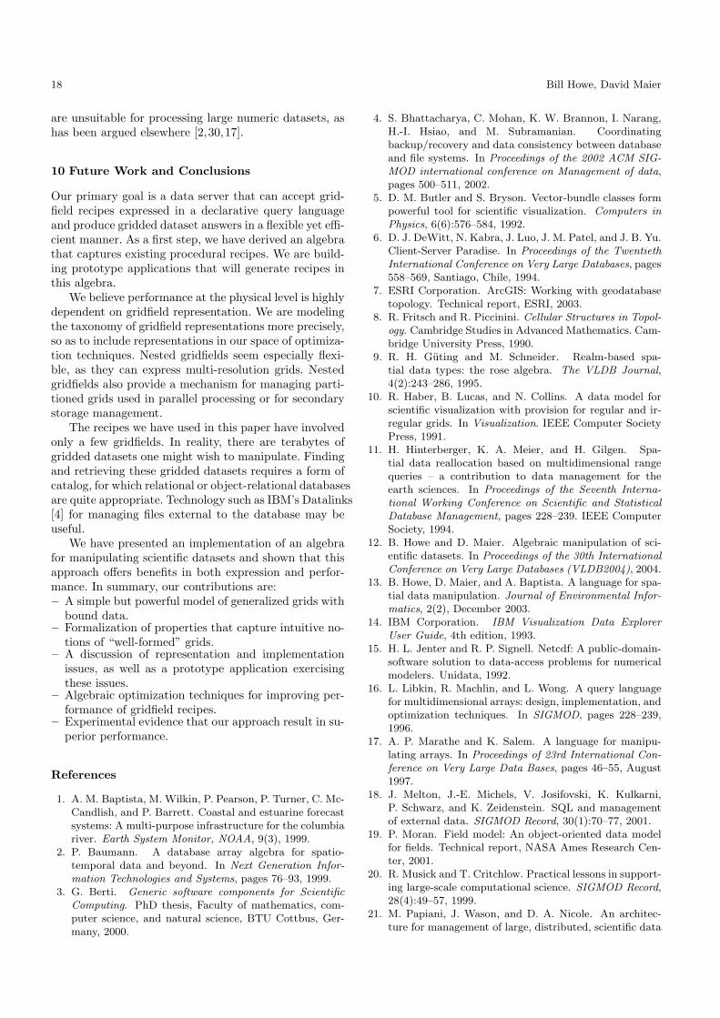
18 Bill Howe, David Maier
are unsuitable for processing large numeric datasets, ashas been argued elsewhere [2,30,17].
10 Future Work and Conclusions
Our primary goal is a data server that can accept grid-field recipes expressed in a declarative query languageand produce gridded dataset answers in a flexible yet effi-cient manner. As a first step, we have derived an algebrathat captures existing procedural recipes. We are build-ing prototype applications that will generate recipes inthis algebra.
We believe performance at the physical level is highlydependent on gridfield representation. We are modelingthe taxonomy of gridfield representations more precisely,so as to include representations in our space of optimiza-tion techniques. Nested gridfields seem especially flexi-ble, as they can express multi-resolution grids. Nestedgridfields also provide a mechanism for managing parti-tioned grids used in parallel processing or for secondarystorage management.
The recipes we have used in this paper have involvedonly a few gridfields. In reality, there are terabytes ofgridded datasets one might wish to manipulate. Findingand retrieving these gridded datasets requires a form ofcatalog, for which relational or object-relational databasesare quite appropriate. Technology such as IBM’s Datalinks[4] for managing files external to the database may beuseful.
We have presented an implementation of an algebrafor manipulating scientific datasets and shown that thisapproach offers benefits in both expression and perfor-mance. In summary, our contributions are:– A simple but powerful model of generalized grids with
bound data.– Formalization of properties that capture intuitive no-
tions of “well-formed” grids.– A discussion of representation and implementation
issues, as well as a prototype application exercisingthese issues.
– Algebraic optimization techniques for improving per-formance of gridfield recipes.
– Experimental evidence that our approach result in su-perior performance.
References
1. A. M. Baptista, M. Wilkin, P. Pearson, P. Turner, C. Mc-Candlish, and P. Barrett. Coastal and estuarine forecastsystems: A multi-purpose infrastructure for the columbiariver. Earth System Monitor, NOAA, 9(3), 1999.
2. P. Baumann. A database array algebra for spatio-temporal data and beyond. In Next Generation Infor-mation Technologies and Systems, pages 76–93, 1999.
3. G. Berti. Generic software components for ScientificComputing. PhD thesis, Faculty of mathematics, com-puter science, and natural science, BTU Cottbus, Ger-many, 2000.
4. S. Bhattacharya, C. Mohan, K. W. Brannon, I. Narang,H.-I. Hsiao, and M. Subramanian. Coordinatingbackup/recovery and data consistency between databaseand file systems. In Proceedings of the 2002 ACM SIG-MOD international conference on Management of data,pages 500–511, 2002.
5. D. M. Butler and S. Bryson. Vector-bundle classes formpowerful tool for scientific visualization. Computers inPhysics, 6(6):576–584, 1992.
6. D. J. DeWitt, N. Kabra, J. Luo, J. M. Patel, and J. B. Yu.Client-Server Paradise. In Proceedings of the TwentiethInternational Conference on Very Large Databases, pages558–569, Santiago, Chile, 1994.
7. ESRI Corporation. ArcGIS: Working with geodatabasetopology. Technical report, ESRI, 2003.
8. R. Fritsch and R. Piccinini. Cellular Structures in Topol-ogy. Cambridge Studies in Advanced Mathematics. Cam-bridge University Press, 1990.
9. R. H. Guting and M. Schneider. Realm-based spa-tial data types: the rose algebra. The VLDB Journal,4(2):243–286, 1995.
10. R. Haber, B. Lucas, and N. Collins. A data model forscientific visualization with provision for regular and ir-regular grids. In Visualization. IEEE Computer SocietyPress, 1991.
11. H. Hinterberger, K. A. Meier, and H. Gilgen. Spa-tial data reallocation based on multidimensional rangequeries – a contribution to data management for theearth sciences. In Proceedings of the Seventh Interna-tional Working Conference on Scientific and StatisticalDatabase Management, pages 228–239. IEEE ComputerSociety, 1994.
12. B. Howe and D. Maier. Algebraic manipulation of sci-entific datasets. In Proceedings of the 30th InternationalConference on Very Large Databases (VLDB2004), 2004.
13. B. Howe, D. Maier, and A. Baptista. A language for spa-tial data manipulation. Journal of Environmental Infor-matics, 2(2), December 2003.
14. IBM Corporation. IBM Visualization Data ExplorerUser Guide, 4th edition, 1993.
15. H. L. Jenter and R. P. Signell. Netcdf: A public-domain-software solution to data-access problems for numericalmodelers. Unidata, 1992.
16. L. Libkin, R. Machlin, and L. Wong. A query languagefor multidimensional arrays: design, implementation, andoptimization techniques. In SIGMOD, pages 228–239,1996.
17. A. P. Marathe and K. Salem. A language for manipu-lating arrays. In Proceedings of 23rd International Con-ference on Very Large Data Bases, pages 46–55, August1997.
18. J. Melton, J.-E. Michels, V. Josifovski, K. Kulkarni,P. Schwarz, and K. Zeidenstein. SQL and managementof external data. SIGMOD Record, 30(1):70–77, 2001.
19. P. Moran. Field model: An object-oriented data modelfor fields. Technical report, NASA Ames Research Cen-ter, 2001.
20. R. Musick and T. Critchlow. Practical lessons in support-ing large-scale computational science. SIGMOD Record,28(4):49–57, 1999.
21. M. Papiani, J. Wason, and D. A. Nicole. An architec-ture for management of large, distributed, scientific data
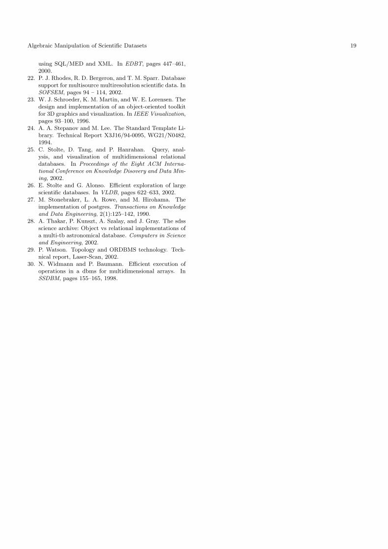
Algebraic Manipulation of Scientific Datasets 19
using SQL/MED and XML. In EDBT, pages 447–461,2000.
22. P. J. Rhodes, R. D. Bergeron, and T. M. Sparr. Databasesupport for multisource multiresolution scientific data. InSOFSEM, pages 94 – 114, 2002.
23. W. J. Schroeder, K. M. Martin, and W. E. Lorensen. Thedesign and implementation of an object-oriented toolkitfor 3D graphics and visualization. In IEEE Visualization,pages 93–100, 1996.
24. A. A. Stepanov and M. Lee. The Standard Template Li-brary. Technical Report X3J16/94-0095, WG21/N0482,1994.
25. C. Stolte, D. Tang, and P. Hanrahan. Query, anal-ysis, and visualization of multidimensional relationaldatabases. In Proceedings of the Eight ACM Interna-tional Conference on Knowledge Disovery and Data Min-ing, 2002.
26. E. Stolte and G. Alonso. Efficient exploration of largescientific databases. In VLDB, pages 622–633, 2002.
27. M. Stonebraker, L. A. Rowe, and M. Hirohama. Theimplementation of postgres. Transactions on Knowledgeand Data Engineering, 2(1):125–142, 1990.
28. A. Thakar, P. Kunszt, A. Szalay, and J. Gray. The sdssscience archive: Object vs relational implementations ofa multi-tb astronomical database. Computers in Scienceand Engineering, 2002.
29. P. Watson. Topology and ORDBMS technology. Tech-nical report, Laser-Scan, 2002.
30. N. Widmann and P. Baumann. Efficient execution ofoperations in a dbms for multidimensional arrays. InSSDBM, pages 155–165, 1998.