Algebraic Manipulation of Scientific Datasets

Bill HoweOGI School of Science & Engineering at

Oregon Health & Science UniversityBeaverton, Oregon

bill@cse.ogi.edu

David MaierOGI School of Science & Engineering at

Oregon Health & Science UniversityBeaverton, Oregonmaier@cse.ogi.edu

Abstract

We investigate algebraic processing strate-gies for large numeric datasets equippedwith a possibly irregular grid structure.Such datasets arise, for example, in com-putational simulations, observation networks,medical imaging, and 2-D and 3-D rendering.Existing approaches for manipulating thesedatasets are incomplete: The performance ofSQL queries for manipulating large numericdatasets is not competitive with specializedtools. Database extensions for processing mul-tidimensional discrete data can only modelregular, rectilinear grids. Visualization soft-ware libraries are designed to process griddeddatasets efficiently, but no algebra has beendeveloped to simplify their use and afford opti-mization. Further, these libraries are data de-pendent – physical changes to data represen-tation or organization break user programs.In this paper, we present an algebra of grid-fields for manipulating both regular and irreg-ular gridded datasets, algebraic optimizationtechniques, and an implementation backed byexperimental results. We compare our tech-niques to those of spatial databases and vi-sualization software libraries, using real ex-amples from an Environmental Observationand Forecasting System. We find that our ap-proach can express optimized plans inaccessi-ble to other techniques, resulting in improvedperformance with reduced programming ef-fort.

Permission to copy without fee all or part of this material isgranted provided that the copies are not made or distributed fordirect commercial advantage, the VLDB copyright notice andthe title of the publication and its date appear, and notice isgiven that copying is by permission of the Very Large Data BaseEndowment. To copy otherwise, or to republish, requires a feeand/or special permission from the Endowment.

Proceedings of the 30th VLDB Conference,Toronto, Canada, 2004

����� ������ �� ������ �

����� ������ ��� !"$#&% '

(�)�* +,�-�. /0�1 23�4�5 6

7�8�9�:;�<�= >?�@ AB�C�D E

FHGJILKMONQPSRTU

V�W XY�Z�[ \

]_^ `a�b�c�d

e�f ghQiJj kl�m�npoqHrSs&t

Figure 1: Datasets bound to the nodes and polygons of a2-D grid.

1 Introduction

Many scientific datasets can be characterized by thetopological structure, or grid, over which they are de-fined. For example, a timeseries might be defined overa 1-dimensional (1-D) grid, while the solution to a par-tial differential equation using a finite-element methodmight be defined over a 3-dimensional (3-D) grid.

These datasets consist of data tuples bound to thecells of a grid. A grid may possess cells of many dimen-sions; data can be associated with the nodes (0-cells),edges (1-cells), polygons (2-cells), and so on. Figure 1shows a 2-D irregular (non-rectilinear) grid with twodatasets bound to it. Geometric coordinates x and yare associated with the nodes of the grid, as are salinityand temperature values. Area and flux values are asso-ciated with each polygon. The grid structure consistsof topological information only – generic cells, and in-cidence and adjacency relationships between cells thatare invariant with respect to a particular geometricembedding. A geometric embedding in this exampleis captured by associating coordinate pairs with thenodes. As these datasets are manipulated and trans-formed, both the grid and the associated data mustbe updated in tandem; new grid-aware operators arerequired. Such operators must handle both regulargrids encoded as multidimensional arrays and irregulargrids that explicitly enumerate their cells. Since thesedatasets tend to be large, efficiency is paramount.

Gridded datasets are especially common in scientificand engineering domains. The context for our inter-est in gridded data is CORIE [1], an Environmental

924

Figure 2: The CORIE grid, extending from the Bajapeninsula to Alaska.

Observation and Forecasting System designed to sup-port scientific and industrial interests in the ColumbiaRiver estuary. The CORIE system both measures andsimulates the physical properties of the estuary, gener-ating 5GB of data and thousands of data products foreach simulation run, including visualizations, aggre-gated results and derived datasets. The data productsare consumed for many purposes, including salmonhabitability studies and environmental impact assess-ments. Figure 2 shows the CORIE domain. The hori-zontal irregular grid extends from the Baja peninsulaup to Alaska to capture the large-scale influences ofthe Columbia River. The Columbia River estuary andthe ocean waters around the mouth of the river (in-set) have a very high density of grid elements, to alsocapture local hydrodynamic processes. Using a verti-cal grid to discretize the depth of the river along withthis large horizontal grid, a 3-D grid can be generated.Time represents a fourth dimension.

Traditional Approaches. Database languagesfor processing multidimensional arrays have been pro-posed [2, 13], but multidimensional arrays cannot di-rectly model irregular grids, such as those used in theCORIE system. A facility to manipulate both reg-ular (rectilinear) grids and irregular (non-rectilinear)grids is missing. Additionally, representing differentdatasets bound to the nodes, edges, and faces of thesame grid is difficult with multidimensional arrays.Raster GIS are similarly unable to model irregulargrids precisely.

Relational databases extended with spatial typescan model irregular grids, but have several weaknesses.Explicit foreign keys and redundant geometric coordi-nates1 can more than double database size. With 5-20GB generated each day, even relatively inexpensivedisk space is at a premium. Transfer times into andout of the database are excessive. Using the bulk loadfacility of Postgres [23], loading one timestep of onevariable (about 800,000 floats) takes over one minute.With six primary variables and 96 timesteps per day,the load time approaches the time to generate the data

1Coordinates of a node are repeated everywhere the node isreferenced.

in the first place on a similar platform. Retrievingdata from the database involves copying tuples to fast,memory-resident structures such as arrays. When re-trieving numeric datasets from a relational database,tuples are usually converted to arrays at the client, in-curring an “impedance mismatch” penalty. The scaleof scientific datasets makes the performance issues as-sociated with impedance mismatch more pronounced[24]. In Section 3.5, we review modeling challengesstemming from storing gridded datasets in relationaldatabases.

Visualization libraries such as the VisualizationToolkit (VTK) [19] provide efficient grid processing,but the routines are highly data dependent and there-fore quite brittle. The library functions also exhibitcomplex semantics, making algebraic properties diffi-cult to derive if they exist. We discuss these issues inmore detail in Section 3.5.

Our Approach. These issues led us to seek a tech-nology that 1) efficiently generates relevant data prod-ucts, 2) reduces programming effort to design and im-plement new data products by allowing manipulationof grid structures directly, 3) integrates neatly withclient tools, especially rendering tools for visualization,and 4) manages topology considerations for both reg-ular and irregular grids transparently.

Our approach has been to devise and implementan algebra specially suited for manipulating griddeddatasets, extending previous work [9]. Our algebraconsists of grids, gridfields, and operators over thesestructures. A gridfield represents the association ofa dataset with a grid. Several gridfields may sharethe same grid; indeed this eventuality allows algebraicidentities important for optimization (see Section 6).Our data model distinguishes topological informationfrom geometric information, handling geometry as or-dinary data attributes. The separation of topologyand geometry allows multiple geometric embeddingsto be handled simultaneously, unlike other data mod-els proposed, e.g., for scientific visualization [5, 8, 15].Some of our operators are analogous to those of rela-tional algebra, but extended to correctly handle thegrid structure. Other operators are specific to grid-fields.

Contributions. We extend previous efforts at de-vising scientific data models [3, 5, 8, 9, 18] by devel-oping algebraic optimizations at both the logical andphysical levels. We contribute a data model and imple-mentation that satisfies the goals above. Specifically:1. The data model captures regular and irregular grids

uniformly.

2. The operators manipulate grid structures directly,avoiding the complexity associated with encodinggrids as assemblies of arrays.

3. The design is well-aligned with client visualizationand analysis tools.

925

4. Our operators admit algebraic identities and conse-quent optimization techniques unique to gridfields.

5. We have tested our data model and implementationon real applications; we present results from theCORIE simulation system.In this paper, we discuss the gridfield model, then

describe data representation, operator implementa-tion, and algebraic optimization of gridfield recipes,a form of query plan. Results are validated via exper-imental comparisons with existing approaches.

2 Related Work

The database community has given multidimensionaldiscrete data (MDD) significant attention over thepast decade. OLAP systems have been extendedwith visualization capabilities [21], but modeling andquerying irregular grids in a relational system is dif-ficult, as we demonstrate. Query languages and pro-cessing techniques based on multidimensional arrays[6, 12, 13, 26] have been developed, but arrays are notthe correct abstraction for general grid manipulations.

Multidimensional arrays capture only rectilineargrids. If, as in the CORIE system, cells in a particulargrid may be triangles, quadrilaterals, or a mix of celltypes, the grid structure is awkward to encode usingarrays. The interpretation of an assembly of arrays asan irregular grid is left to the application, undermin-ing data independence. Further, we encounter multi-ple datasets bound to the same grid, but perhaps tocells of different dimension. Using arrays, the relation-ship between these datasets is lost; each must use itsown distinct “spatial domain” [2]. Finally, the topol-ogy suggested by these grids is always implicit, makingit difficult to separate geometry from topology. Thiscapability is required when attempting to support twogeometric embeddings of the same grid simultaneously,e.g., into different coordinate systems.

Several higher-level data models for scientific datahave been proposed that capture both regular and ir-regular grids, and some separate topology from geom-etry [3, 5, 8]. However, algebraic manipulation of gridstructures is not supported and experimental resultsare not reported.

Others have demonstrated that relational databasesdo not scale up to handle large scientific datasets[16, 22]. One proposed solution is to treat scientificdatasets as external data sources, and access themusing the SQL standard for management of externaldata (SQL-MED) [14]. Papiani et al. [17] report somesuccess applying the standard to manage turbulencesimulations.

Designers of spatial database systems are becom-ing aware that topological “connection” informationcan be as important as geometry for modeling andquery processing. ESRI’s ArcGIS version 8.3 [7] in-cludes topology information modeled as integrity rules.

a

bc

A

1

2B

a1

b1

c1

a2

b2

c2

G = A ⊗⊗⊗⊗ B

Figure 3: The cross product of two simple grids.

Users can express the rule that every polygon repre-senting a building must be explicitly connected to aline segment representing a road. ESRI’s product alsosupports raster data manipulation using a Map Alge-bra, but irregular grids are difficult to model preciselyas raster data. Laser-Scan has produced a topology-enabled GIS extension for Oracle called Radius [25].They allow nodes to be snapped together to expresstopological relationships independently of geometricembeddings. However, there is no notion of a ma-nipulable gridded dataset, and therefore, our Goals 2and 3 are not met.

3 The Gridfield Algebra

Grids are constructed from sets of k-dimensional cells.We refer to a cell of dimension k as a k-cell, followingthe topology literature [3]. Intuitively, a 0-cell is apoint, a 1-cell is a line segment (or poly-line), a 2-cell isa polygon, and so on. These geometric interpretationsof cells guide intuition, but a grid does not explicitlyindicate its cells’ geometry.

Nodes and Cells. We will refer to a 0-cell as anode. A node is named, but is otherwise featureless. Ak-cell c is a set of nodes (c0, c1, . . . , cn), where k < n.The order of the nodes allows interpretation of cellsas visual shapes, but is not strictly necessary in themodel. For example, a 1-cell must refer to at least twonodes, but can refer to more. Let N(c) be the nodesof a cell c viewed as a set. We say a cell c is incidentto a cell d if N(c) ⊆ N(d). The dimension k of a k-cellc is written dim(c).

Node sets and the incidence relationship are suffi-cient to encode some topological relationships. Twocells are adjacent if they share nodes but neither is in-cident to the other. Two cells are connected if they ap-pear in the transitive closure of the adjacency relation-ship. A topological distance measure can be definedby counting the number of cells traversed through theadjacency relationship to reach another cell. Note thatcontainment and overlap are geometric relationships,since they depend on a particular geometric embed-ding.

Namespaces. Nodes are referenced with respectto a namespace. For example, nodes can be named bytheir physical position within an array. Let L be a setof labels and C be a set of nodes. A namespace is a 1-1function h : C → L. Cell equality is only defined withrespect to a particular namespace. Cells in differentnamespaces are assumed to be unequal.

926

3.1 Grids

A grid is a sequence of sets of cells,[G0, G1, G2, . . . , Gd], where each set Gi containscells of dimension i. A non-empty grid must havea non-empty set of 0-cells (nodes). The dimensionof a grid G is the greatest i such that Gi is non-empty. A grid’s dimension is written dim(G). InFigure 1, the grid has four 0-cells, six 1-cells, andthree 2-cells, and it therefore has dimension 2. Notethat a d-dimensional grid G must have a non-emptycomponent Gd, but may have an empty componentGi for 0 < i < d.

This definition is very general; a grid may be a col-lection of unconnected polygons for GIS data, a setof scattered points for values of a random variable, ora well-connected graph modeling the truss structureof a bridge. The grids in our application are used todiscretize the Columbia River estuary, for solving the3-D transport equations via a finite-element method.

We can define set-like operations on grids with re-spect to a namespace to test cell equality. The in-tersection of two grids G and F is the component-wise intersection of the sets Gi and Fi. That is,G ∩ F = [G0 ∩ F0, G1 ∩ F1, . . . ]. Union and differencecan be defined similarly.

Grids must be well-formed ; no cell in Gi may refer-ence a node not in G0, for 0 < i ≤ dim(G). Operationson grids must preserve well-formedness. If nodes areremoved from a grid, then cells that reference thosenodes must also be removed.

Cross Product. The cross product of two gridsgenerates a higher-dimensional grid based on crossproducts of their constituent sets. The node productof two 0-cells a and b is written ab. The result is a0-cell x in a new namespace. The cell product of acell c = (c1, c2, . . . , cn) and a cell d = (d1, d2, . . . , dm),written c × d, is a cell e with dim(e) = dim(c) +dim(d) such that e = (c1d1, c1d2, . . . , c1dm, c2d1, c2d2,. . . , c2dm, . . . , cnd1, cnd2, . . . , cndm).

Figure 3 shows an example of the cross product.The cross product of grids A and B contains six 0-cells,nine 1-cells, five 2-cells, and one 3-cell. The 3-cell isthe interior of the prism, the 2-cells are the three rect-angular faces and the two triangular bases, the 1-cellsare the edges, and the 0-cells are the vertices.

We capture all these cases using the set-theoreticcross product of the components of the grids A andB. For example, the 3-cell prism in G is generated bysweeping the triangle of A through a third dimensiondefined by the line segment of B. This constructioncan be expressed as the cross product of the 2-cells ofgrid A (A2) and the 1-cells of grid B (B1). The rect-angular faces are generated by sweeping the 1-cells ofA through the space defined by the 1-cell of B. Again,the construction is expressed as the cross product of

A1 and B1. More precisely, the cells of G are given by

G0 = A0 ×B0

G1 = (A1 ×B0) ∪ (A0 ×B1)G2 = (A2 ×B0) ∪ (A1 ×B1)G3 = A2 ×B1

Evaluating these expressions, we obtain

G0 = {a1, b1, c1, a2, b2, c2}G1 = {(a1, b1), (b1, c1), (c1, a1), (a2, b2),

(b2, c2), (c2, a2), (a1, a2), (b1, b2), (c1, c2)}G2 = {(a1, b1, c1), (a2, b2, c2),

(a1, a2, b1, b2), (b1, b2, c1, c2), (c1, c2, a1, a2)}G3 = {(a1, a2, b1, b2, c1, c2)}

In general, let A = [A0, A1, . . . , Aa] and B =[B0, B1, . . . , Bb] be grids. The cross product of A andB, written A⊗B, is a grid [G0, G1, . . . , Gd] such thatGk =

⋃kj=0 Aj ×Bk−j for 0 ≤ k ≤ a + b.

We have used the cross product operator frequentlyin expressing the data products of the CORIE system.The 3-D CORIE grid is the cross product of a 2-D hor-izontal grid and a 1-D vertical grid. The time dimen-sion can be incorporated with another cross product.Note that simpler rectilinear grids can be modeled asthe cross product of two 1-D grids. By commutingother operations through the cross product, we canreduce its complexity or remove it altogether. Toolsthat do not provide an explicit cross product operatordo not have access to these optimizations, as we shallsee.

3.2 Gridfields

When data is bound to a grid, the grid becomes agridfield. Formally, a gridfield G is a triple (G, k, f),where G is a grid, k is a non-negative integer, and f isa function Gk → τ for some type τ . The integer k iscalled the rank and can be extracted from a gridfieldG by writing rank(G). The type of a gridfield is thereturn type τ of its function component f , writtenG : τ . We will generally use only primitive numerictypes and tuples of primitive numeric types as returntypes.

Earlier we used a trussed bridge as an example ofa grid. Gridfields defined over such a grid might re-turn the net force at each node, or the linear forcealong each truss. Gridfields capture both cases natu-rally by binding data to 0-cells or 1-cells, respectively.Images can be viewed naturally as a gridfield definedover 2-cells of a rectilinear grid. We can also modelunstructured sets as a gridfield over a grid consistingsolely of 0-cells.

To support multiple geometric embeddings, geo-metric information is modeled as ordinary data valuesbound to the cells of a grid. A simple example is a

927

(a) (c)(b)

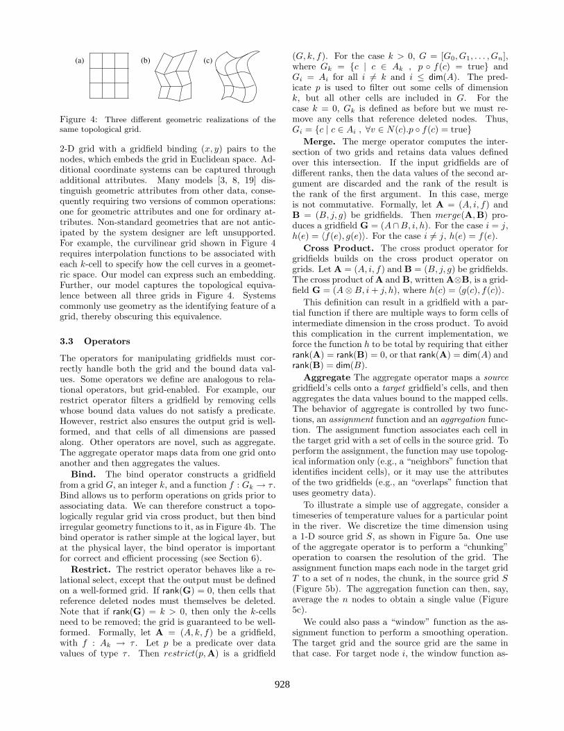
Figure 4: Three different geometric realizations of thesame topological grid.

2-D grid with a gridfield binding (x, y) pairs to thenodes, which embeds the grid in Euclidean space. Ad-ditional coordinate systems can be captured throughadditional attributes. Many models [3, 8, 19] dis-tinguish geometric attributes from other data, conse-quently requiring two versions of common operations:one for geometric attributes and one for ordinary at-tributes. Non-standard geometries that are not antic-ipated by the system designer are left unsupported.For example, the curvilinear grid shown in Figure 4requires interpolation functions to be associated witheach k-cell to specify how the cell curves in a geomet-ric space. Our model can express such an embedding.Further, our model captures the topological equiva-lence between all three grids in Figure 4. Systemscommonly use geometry as the identifying feature of agrid, thereby obscuring this equivalence.

3.3 Operators

The operators for manipulating gridfields must cor-rectly handle both the grid and the bound data val-ues. Some operators we define are analogous to rela-tional operators, but grid-enabled. For example, ourrestrict operator filters a gridfield by removing cellswhose bound data values do not satisfy a predicate.However, restrict also ensures the output grid is well-formed, and that cells of all dimensions are passedalong. Other operators are novel, such as aggregate.The aggregate operator maps data from one grid ontoanother and then aggregates the values.

Bind. The bind operator constructs a gridfieldfrom a grid G, an integer k, and a function f : Gk → τ .Bind allows us to perform operations on grids prior toassociating data. We can therefore construct a topo-logically regular grid via cross product, but then bindirregular geometry functions to it, as in Figure 4b. Thebind operator is rather simple at the logical layer, butat the physical layer, the bind operator is importantfor correct and efficient processing (see Section 6).

Restrict. The restrict operator behaves like a re-lational select, except that the output must be definedon a well-formed grid. If rank(G) = 0, then cells thatreference deleted nodes must themselves be deleted.Note that if rank(G) = k > 0, then only the k-cellsneed to be removed; the grid is guaranteed to be well-formed. Formally, let A = (A, k, f) be a gridfield,with f : Ak → τ . Let p be a predicate over datavalues of type τ . Then restrict(p,A) is a gridfield

(G, k, f). For the case k > 0, G = [G0, G1, . . . , Gn],where Gk = {c | c ∈ Ak , p ◦ f(c) = true} andGi = Ai for all i 6= k and i ≤ dim(A). The pred-icate p is used to filter out some cells of dimensionk, but all other cells are included in G. For thecase k = 0, Gk is defined as before but we must re-move any cells that reference deleted nodes. Thus,Gi = {c | c ∈ Ai , ∀v ∈ N(c).p ◦ f(c) = true}

Merge. The merge operator computes the inter-section of two grids and retains data values definedover this intersection. If the input gridfields are ofdifferent ranks, then the data values of the second ar-gument are discarded and the rank of the result isthe rank of the first argument. In this case, mergeis not commutative. Formally, let A = (A, i, f) andB = (B, j, g) be gridfields. Then merge(A,B) pro-duces a gridfield G = (A∩B, i, h). For the case i = j,h(e) = 〈f(e), g(e)〉. For the case i 6= j, h(e) = f(e).

Cross Product. The cross product operator forgridfields builds on the cross product operator ongrids. Let A = (A, i, f) and B = (B, j, g) be gridfields.The cross product of A and B, written A⊗B, is a grid-field G = (A⊗B, i + j, h), where h(c) = 〈g(c), f(c)〉.

This definition can result in a gridfield with a par-tial function if there are multiple ways to form cells ofintermediate dimension in the cross product. To avoidthis complication in the current implementation, weforce the function h to be total by requiring that eitherrank(A) = rank(B) = 0, or that rank(A) = dim(A) andrank(B) = dim(B).

Aggregate The aggregate operator maps a sourcegridfield’s cells onto a target gridfield’s cells, and thenaggregates the data values bound to the mapped cells.The behavior of aggregate is controlled by two func-tions, an assignment function and an aggregation func-tion. The assignment function associates each cell inthe target grid with a set of cells in the source grid. Toperform the assignment, the function may use topolog-ical information only (e.g., a “neighbors” function thatidentifies incident cells), or it may use the attributesof the two gridfields (e.g., an “overlaps” function thatuses geometry data).

To illustrate a simple use of aggregate, consider atimeseries of temperature values for a particular pointin the river. We discretize the time dimension usinga 1-D source grid S, as shown in Figure 5a. One useof the aggregate operator is to perform a “chunking”operation to coarsen the resolution of the grid. Theassignment function maps each node in the target gridT to a set of n nodes, the chunk, in the source grid S(Figure 5b). The aggregation function can then, say,average the n nodes to obtain a single value (Figure5c).

We could also pass a “window” function as the as-signment function to perform a smoothing operation.The target grid and the source grid are the same inthat case. For target node i, the window function as-

928

12.1°C12.6°C 13.1°C 13.2°C 12.8°C 12.5°C

{12.6°C, 13.1°C, 13.2°C}

{12.8°C , 12.5°C , 12.1°C}

12.95°C 12.45°C

a)

Assignment

Aggregation

b)

c)

Figure 5: (a) A 1-D gridfield returning temperatures. (b)Assignment to the target grid T . (c) Aggregation usingarithmetic mean.

signs source nodes [i−k, i−k+1, . . . , i, i+1, . . . , i+k].The aggregation function could be anything, but forsmoothing, an arithmetic or weighted mean seems ap-propriate. We have used a 1-D example for illustra-tion, but multidimensional window and chunking func-tions are common.

Formally, let T = (T, k, f) and S = (S, j, g) be grid-fields, where f : Tk → α and g : Sj → β. Let m bea function m : Tk → P(Sj). Let a : P(β) → γ be afunction for some type γ. Then aggregate(T,m, a,S)produces a gridfield G = (T, k, h) where h(c) =a({g(e) | e ∈ m(c)}).

3.4 Benefits

We summarize the benefits of our data model:• Grids are first-class and of arbitrary dimension.• Grids can be shared between datasets.• Geometry is modeled as data, exposing topologi-

cal equivalences between geometric interpretations;e.g., different coordinate systems.

• Data can be associated with cells of any dimension,avoiding ambiguities arising from associating, forexample, cell areas with nodes.

• The data model captures irregular grids directly,but the cross product operator expresses the reg-ularity of rectilinear grids.

• The aggregate operator is extensible, allowingapplication-specific assignment and aggregationfunctions.

• The operators obey algebraic identities enabling op-timization (see Section 6).

• Client programs can process grids without intricatearray manipulations.

3.5 Detailed Example

Many of the CORIE datasets are defined over a 3-Dgrid constructed as the cross product of a 2-D irreg-ular grid and a 1-D grid. The 2-D grid H describesthe domain parallel to the earth’s surface, a horizon-tal orientation. The 1-D grid V extends in a verticaldirection perpendicular to the earth’s surface. Thesegrids are illustrated in Figures 2 and 6, respectively.

Although the simulation code operates over the gridformed from the cross product of H and V , the output

Figure 6: The vertical grid and the river’s bathymetry inthe CORIE domain.

datasets are produced on a reduced grid. To see why,consider Figure 6. The shaded region illustrates thebathymetry of the river. The horizontal grid is definedto cover the entire surface of the water. Below the sur-face, some nodes in the full 3-D cross product grid arepositioned underground! The simulation code outputsonly valid, “wet,” data values to conserve disk space.Therefore, we must define this “wet” grid to obtain anadequate description of the topology of the data. Thebathymetry data can be modeled as a gridfield overthe horizontal grid H, associating a depth with eachnode. To filter out nodes in the product grid G thatare deeper than the river bottom, we need to comparethe node’s depth (bound to V ) with the bottom depth(bound to H). In the following, we will refer to a rank0 gridfield H constructed from the 2-D horizontal gridH and attributes x, y, b. The attribute b captures theriver’s bathymetry at a particular location. We willalso refer to a rank 0 gridfield V constructed from the1-D vertical grid V and an attribute z.

The task is to construct the grid over which thesimulation outputs are defined, bind a dataset to it,and visualize the results. The recipe for this task isshown in Figure 7. Each gray oval is an operator inour algebra. The unfilled oval at the right representsa client task: render the grid as an image. The recipebegins at left with the H and V gridfields. The crossproduct operator produces a different, 3-D gridfield.After using restrict to filter out the river bottom, wehave our “wetgrid” (at the point labelled in Figure7). After binding a salinity dataset to the wetgrid, werestrict the grid to a user-supplied region. The term“region” is shorthand for a bounding-box conditioninvolving x, y, and z.

Using a Relational Database. Our initial at-tempt to manage the CORIE datasets was to loadthem into a relational table and manipulate them us-ing SQL. The first task is to devise a schema that cap-tures both the grid and the data. One method is tostore each logical gridfield as a separate relation: oneattribute stores the cells to which the data is bound,while the other attributes store the bound data. Aproblem with this approach is that each scalar datasetbound to a grid is modeled as an attribute of a re-lation. New datasets are generated daily. To captureeach new dataset, we can either extend the existing ta-ble with an additional attribute or add the new dataset

929

⊗

H : (x,y,b)

V : (z)

r(z>b) b(s) r(region) render

� � � � � � � � �

Figure 7: A recipe for visualizing a 3-D CORIE dataset.

as a separate table. Either way, we are changing thedatabase schema daily, making robust queries difficultto write.

A better strategy for modeling grids and gridfieldsusing an RDBMS is to allow any number of datasetsto be bound to the same grid. The relation grid storesmetadata about the grid. Each grid is associated witha number of cells of varying dimension, stored in therelation kcell. Tuples in the values relation are boundto cells using foreign keys, perhaps integers. Now noschema changes are required to insert new datasets,but binding a particular dataset to its grid involvesa join between the kcells relation and the values rela-tion using the ordinal. Including the bound cell’s def-inition itself in the value relation seems to avoid thejoin. However, working with multiple bound datasetssimultaneously requires a self-join on the cell columnfor each dataset. Computing joins on these complexcolumns is more expensive than computing joins on aninteger column.

To associate cells with data values, we already musthave computed the appropriate grid. However, it isvaluable at times to store grids intensionally; that is,decomposed. For example, a frequently used CORIEgrid is the cross product of the horizontal grid H andthe vertical grid V . Although a relational approachallows us to express the cross product as a query, wecannot declare that the tuples in a physical table havea foreign key to a query result. An alternative is to usea 2-part foreign key, where the first part references acell in the grid H, and the second part references a cellin the grid V . Now the space required is higher, anddatasets bound to cross-product grids are accessed dif-ferently from other datasets. Precomputing and stor-ing an intensional grid consumes space and obscuresthe relationship between the composed grid and itsbase grids.

Using Visualization Software. Another ap-proach, which sacrifices data management capabilitiesfor a richer toolset, is to use a visualization libraryspecifically designed to work with gridded datasets.Such libraries are usually oriented toward workingwith a single dataset at a time, and therefore pro-vide little support for reasoning about the relation-ships between datasets. Unfortunately, recognizingand exploiting relationships between datasets is a greatsource of optimization opportunities, as we show later.Further, the programmer is under a significant burdenin making use of the library, as each tool has compli-cated and nuanced semantics.

Software libraries provide functions (or objects) for

each specific task. The programmer is often askedto choose between two similar functions that differonly in the type of data on which they operate or theparticular algorithm they implement. For example,in the Visualization Toolkit [19], to extract a subsetof a grid, there are a variety of functions to choosefrom. The operation vtkExtractUnstructuredGridaccepts internal ids of points and cells, or a func-tion over the geometry of the points. The operationvtkExtractGrid works only on structured grids andaccepts i, j, and k index ranges that define a struc-tured subgrid. The operation vtkExtractGeometryworks on a wider range of datasets, but accepts onlygeometric functions rather than topological ids. Amore efficient version is available for polygonal data,vtkExtractPolyDataGeometry. Another operator,vtkThreshold filters grids based on non-geometric at-tributes.

The physical concerns of representations and algo-rithms are intermingled with semantic concerns suchas which data is used to filter the grid. All of the op-erations above can be implemented using the restrictoperator, possibly with the aggregate operator to eval-uate complex geometric functions. The distinction be-tween filtering geometric data and other bound datais removed in our model.

As we gained experience with VTK and anothervisualization library [10], we found that simple con-cepts we used to describe our data products often didnot have counterparts in these libraries. Below we listsome specific concepts we found weak or missing.• Cross Product Grids.• Shared Grids.• Combinatorial algorithms. Berti observes that com-

binatorial algorithms for grid manipulation are su-perior to geometric algorithms [3].

• Aggregation. Both libraries we reviewed implementparticular instances of aggregation, but do not pro-vide a general aggregation abstraction.

• Time. We found it useful to reason about time sim-ilarly to other dimensions.

• Irregular Grids. Manipulating regular grids is eas-ier than manipulating unstructured grids. SinceCORIE involves both kinds of grids, we sought aunifying model.

4 Gridfield Representations

A goal of this work is to support and exploit multiplerepresentations of gridfields, for two reasons: First,supporting a variety of representations can promoteinteroperability with existing systems. Second, no onerepresentation is efficient for all recipes.

We have identified four major patterns of gridfieldrepresentation used in practice. The tabular repre-sentation forms 〈cell, value〉 tuples, making it easy to

930

attributesk

…

Grid

Gk GdG0

…

… …

… …

Hcellposition

cell

Hash

Figure 8: Internal representation of a gridfield in our cur-rent implementation.

pipeline data from one operator to another, but diffi-cult to separate grid from data.

The parallel representation uses a separate arrayfor each attribute, all aligned positionally with an-other array for the cells to which the attributes arebound. With this representation, binding in new at-tributes and projecting out unneeded ones are trivialoperations.

The decomposed representation stores gridfields in-tensionally, requiring the client program to assemblethe gridfield as needed. Cross product grids are oftendecomposed in order to save space.

The nested representation involves gridfield at-tributes that can themselves be gridfields. A 4-D time-space gridfield may be a timeseries (the outer grid) anda 3-D spatial grid (the inner, nested grid).

Our Representation. Figure 8 illustrates the rep-resentation we use in our current implementation. Thegridfield at top stores an integer rank k, and pointersto the grid and each attribute. An attribute is an ar-ray of data values, and a grid is a sequence of arraysof cells. Cells of dimension k are aligned positionallywith the attributes; we use the parallel representationdescribed above. We began with the parallel represen-tation because it exhibits good performance charac-teristics (see Section 8) and is used frequently in clientsoftware [10, 19] and standard file formats (cf. [11]).

A hash index (H in Figure 8) maps cell definitionsto their ordinal position. This index allows the func-tion semantics prescribed by the model to be evalu-ated in constant time on average. A cell definitionis mapped to an array index, which is then used tolookup a data value in each of the attribute arrays.The hash function used maps each cell to its first node,exploiting the fact that seldom do more than 4 or 5cells touch any one node. Our tests show that thishash function generates very few collisions while offer-ing fast evaluation time.

Another index (not shown in Figure 8) speeds upnavigation of the incidence relationship. Each node inthe grid is mapped to the cells to which it is incident.The aggregate operator frequently uses this index.

5 Operator Implementation

Our operators are implemented in C++, with in-memory indices implemented using the Standard Tem-plate Library (STL) [20]. Physical recipes are cur-rently constructed by hand, though we are designing adeclarative query language as an interface to the phys-ical operators.

The parallel representation improves performancein some cases. Binding a new attribute to a grid isinexpensive, as is projecting out attributes. We neednot iterate of the arrays; we can simply make a copy ofthe gridfield header structure (see Figure 8) containingpointers to the information we want.

The merge operator might compute the intersec-tion of two grids during evaluation, and is thereforepotentially expensive. However, if the two argumentgridfields are defined over the same grid, merge canbe evaluated in constant time. Since gridfields mayshare grids via pointers, checking for grid equivalenceis essentially free.

The aggregate operator admits specialized imple-mentations for syntactic convenience and to exploit ef-ficient algorithms. The apply specialization uses iden-tical source and target grids, but applies an arithmeticexpression to the data values. The project specializa-tion also uses identical source and target grids, butsimply removes attributes from each logical tuple. Theaffix operator changes the rank of a gridfield by trans-ferring the data values to cells of a different dimensionand averaging. The unify operator aggregates all ofthe values in a grid, binding the result to the unit gridconsisting of a single node.

Cross product is usually the most expensive opera-tor in the algebra. In the next section, we investigatealgebraic rewrites to reduce its cost or remove it al-together. We can also improve its implementation insome cases. The cross product of a grid with nodes,edges, and polygons and a grid with nodes and edgesproduces nodes, edges, polygons, and polyhedra. How-ever, for visualization purposes, we may only need thepolyhedra and the nodes; cells of intermediate dimen-sions need not be computed. However, to use such a“prune” implementation, we must be able to determinewhich dimension cells will be consumed downstream.

Another implementation of the cross product oper-ator (applicable to Figure 7) exploits the fact that it isfollowed immediately by a restrict. In relational alge-bra, a join is semantically equivalent to a cross prod-uct followed by a restrict. We can create an analogous“join” operator that evaluates the restrict as the crossproduct is computed, computing fewer cells overall.

6 Optimization

Having described our data representation and opera-tor implementation, we now present optimization tech-niques enabled by our algebra for improving the per-

931

⊗

��������� � ���

������������������ �"!�#$�%�&(')* +�,�-/.

021�35476 8:9<; =

>@?�A<BDC

Figure 9: An optimized recipe for visualizing a 3-DCORIE dataset.

formance of recipes. Our examples are actual CORIEdata products, though the techniques we use generalizeto any domain involving irregular grids, cross productgrids, or selected sub-regions.

Forward Binding. The recipe in Figure 7 com-putes a 3-D salinity gridfield, then restricts the resultto a user-specified region. The logical model allows usto freely commute the restrict operator with the bind,and then with the cross product [9], to significantlyreduce the size of the intermediate results. However,the physical implementation materializes functions asarrays, so special handling is required. The array wewish to bind can only be correctly interpreted usingthe ordinal positions of the wetgrid. If we push therestrict earlier, we will produce a grid smaller thanthe wetgrid, and the bound array will be misaligned.To solve this problem, we can pre-compute the ordinalpositions of cells in the wetgrid and record these valuesin an attribute. This attribute can then be passed tothe bind operator and used as offsets into the array ondisk.

Our goal is to push the restrict on “region” beforethe cross product, but there are two obstacles. Oneis the cross product itself, and the other is anotherrestrict involving attributes b and z from H and V,respectively2. A cell’s ordinal position in a cross prod-uct grid can be derived from the ordinal positions ofthe cells used to construct it. However, the grid wewant is not just a cross product of two grids, but therestriction of a cross product. Therefore, the ordinalsof the cells of the wetgrid are dependent on the condi-tion used to filter out the “dry” cells.

In the general case, the 1000th cell in the grid priorto a restrict could be the 1st cell or the 1000th cellin the restricted grid. However, we know a physicalproperty of the gridfield V: It is sorted on the at-tribute z. We can therefore compute the positions ofthe wetgrid’s cells without actually materializing thegrid itself.

Recall the attribute b of the gridfield H storesbathymetry information for the river. Specifically, bis an index into the gridfield V. Since V is sorted onz, we can use b to determine the number of cells ineach vertical column of water. With these cell counts,we can compute an offset into the array to be boundto the wetgrid.

The result of these transformations is the optimizedrecipe shown in Figure 9. The potentially highly se-lective restricts on x, y and z are evaluated prior to

2This restrict compares attributes from both H and V anddoes therefore not commute with the cross product.

a)

b)

Figure 10: (a) A vertical slice data product. (b) A hori-zontal slice data product.

the cross product.Lowering Dimensionality Two common 2-D

CORIE data products are horizontal and vertical“slices.” Examples of these data products for the salin-ity variable are shown in Figure 10. One way to expressthe horizontal slice data product is to use the samerecipe as in Figure 7, but restrict the z dimension toa single node. As before, we could push the restrictsthrough the cross product. This time, though, we ob-serve that restricting V to a single node produces theunit grid. The unit grid is the identity for the crossproduct operator, up to namespace isomorphism. Wecan therefore remove the cross product operator alto-gether.

This optimization is unavailable to systems thatcannot reason about grids algebraically. We have notonly produced a faster recipe, but we have also natu-rally expressed a critical correctness criteria: The out-put grid is 2-D. Although the wetgrid is constructedfrom prism-shaped cells, this data product is definedover triangles. (We have assumed that the depth atwhich a slice is to be taken corresponds to one of thedepths in the vertical grid V . We could relax thisassumption by using an aggregate operator equippedwith an interpolation function.)

Computing a vertical slice is more difficult. Thehorizontal grid H has an irregular topology consist-ing of triangles. To take a vertical slice, we must stillproject the 3-D grid down to two dimensions, but thetarget is a new grid not appearing elsewhere in therecipe. Consider a user who wants to view a verticalprofile of the salinity intrusion along a deep channelnear the mouth of the estuary. To specify “along adeep channel” to the system, the user selects a se-quence of points in the xy plane, as shown in Figure11a. We can connect these points to form a 1-D grid,P . A cross product with the vertical grid gives us a2-D slice, P ⊗ V (Figure 11b).

Using VTK, we must manually construct the gridP ⊗ V producing points in 3-D space. For each point,we must search in the 3-D wetgrid for the cell thatcontains the point, then perform a 3-D interpolation

932

���������⊗ ��� ������������������ �"!�#%$'&)( *,+.-

/1032547698�:5;=<�>

?A@CBEDGF�H�I.J�K,L.MONQP.RTSVUW�X%Y)Z1[V\']_^�`%a.b)ced,f.g_h

ikj�l�mon⊗ prq

Figure 11: Four intermediate steps in an efficient “verticalslice” recipe.

of salinity values.With the gridfield algebra, we can do the work in

two dimensions for considerable savings. Each pointin P can be positioned in a triangle in the horizontalgrid H. We can restrict H to only those cells thatcontain one or more points in P using the aggregateoperator followed by a restrict, producing a grid M(Figure 11c).

Since the grid M is a restriction of the grid H, wecan use forward binding (as we did previously) to con-struct a 3-D grid (not shown in Figure 11) and bind theappropriate salinity values to it. We can now performthe same search-and-interpolate operation required byVTK, but using a much smaller 3-D grid.

An additional optimization is possible. Instead ofconsidering V as a 1-D grid, we prune the 1-cells,leaving only the nodes. Call this grid V ′. The gridM ⊗ V ′ consists of “stacks” of 2-D triangles (Figure11d), rather than a connected set of 3-D prisms. In-terpolation using triangles is much cheaper than inter-polation using prisms, further reducing the cost.

By working primarily in two dimensions, we wereable to produce a less expensive recipe. Lowering thedimension of the intermediate results saves time sincea) higher dimensional gridfields tend to have morecells, and b) algorithms for manipulating 3-D cells aremore expensive than their 2-D counterparts.

Merging Related Grids The plume is the regionof water beyond the mouth of the river with a salt con-tent below a given threshold. The recipe to computethe plume extends the recipe to bind salinity to thewetgrid in Section 6. We encode the definition of theplume as conditions passed to the restrict operator.

Consider a recipe to find the portion of the plumeabove a certain temperature. Assume temperaturedata has been bound, separately, to another instanceof the wetgrid, and we now need to merge this datawith the salinity gridfield.

We need to evaluate two restrict operators (r) andone merge operator (m) to obtain the correct gridfield.Three versions of the relevant fragment of this newrecipe are shown in Figure 12. Figure 12a shows thetwo restricts evaluated after the merge. Previously, weimproved performance by evaluating restricts early, as

�

���

������� ��������

������� ��� �

�� �!#"

$&%

'�(�)+*-, .�/�0�1�2

3#4+576 8

9;:

<>=�?@�A B�C�D�E�FG�HI7J

K�LNMPO

Figure 12: Three equivalent sub-recipes. (a) Restrict op-erations are combined into one. (b) The restrict operatorsare pushed through a merge, resulting in a less efficientplan. (c) Evaluating one restrict at a time might requireless memory.

in Figure 12b. In this case the merge operator mustcompute the intersection of two grids – an O(nm) al-gorithm, where n and m are the number of cells in Sand T, respectively. But observe that in Figure 12a,both arguments are defined over the same grid. Thisknowledge allows the merge to be evaluated trivially.The recipe in Figure 12c may also be a good choice.Since the grid T is known to be a subset of the grid S,we can still evaluate the merge in constant time. Wecan also evict the attribute t from memory right afterwe have evaluated the first restrict, possibly loweringthe memory footprint of the overall recipe.

7 Experimental Results

We performed experiments to 1) validate our designchoices in the physical implementation and 2) to deter-mine whether algebraic optimization techniques couldimprove performance over more traditional solutions.

The experiments were run on a dual 2.4 GHz pro-cessor with 4GB of RAM. This machine is nearly iden-tical to one node of the cluster on which the CORIEsimulations are executed. Each experiment involved5 trials, and three experiments were done at differenttimes. The samples produced a variance of less than1% of the mean, demonstrating stability.

The CORIE horizontal grid consists of 29,602 nodesand 55,081 2-cells. The vertical grid has 62 nodes and61 1-cells. The wetgrid has 829,852 nodes, and there-fore each timestep of each dataset has 829,852 values.

Our first experiment compared physical implemen-tations of the cross product operator. The “prune”implementation avoids extra work by computing onlythe nodes and polyhedra of the 3-D cross product. The“join” implementation composes the cross product andsubsequent restrict. Figure 13 shows results for theoriginal cross product implementation (“no opt”), the“prune” implementation (“prune”) and with both im-provements (“both”). If Cw and Cr are the cardinali-ties of the wetgrid and the result gridfield, respectively,then the selectivity (x-axis) is 1− Cr

Cw.

Times reflect overall execution time of the 3-Dscalar data product described in Section 3.5, highlight-ing the cross product operator’s significant cost rela-tive to the other operators in the recipe. The graphshows that avoiding cell materialization does indeed

933

0

5

10

15

20

25

30

0 0.2 0.4 0.6 0.8 1selectivity

tim

e (s

ecs)

no opt

prune

both

Figure 13: Comparing implementations of the cross prod-uct operator.

improve performance. On average, the prune imple-mentation results in 35% faster times than comput-ing the full cross product. The join implementationdoes not provide a consistent improvement. With thestandard cross product implementation, we can pre-dict precisely the space requirements of the output.With the join implementation, we must estimate theselectivity of the join condition and dynamically re-size arrays when we are wrong. Although the joinimplementation produces no unnecessary cells, the ex-tra complexity of memory management washes out theperformance gain.

The second experiment compares our algebraicallyoptimized recipe in Figure 9 with the unoptimizedrecipe in Figure 7, as well as with two more traditionalapproaches. First, we used a relational database ex-tended with spatial data types to represent the cells.Second, we used VTK along with custom code thathandles those operations inexpressible in VTK.

The relational approach uses SQL to join data withcells and select the “wet” values. Our test DBMS wasPostgres [23], configured appropriately for the largemain memory of our experiment platform.

The times for the relational approach are artificiallylow, as we did not include the time to extract the re-sults to the client. Instead, the results were simplyloaded into a temporary table on the server. We feltthat the diversity of potential client interfaces muddlesthe results, and a query-only experiment represents aconservative lower bound. For our own approach, wedid include the time required to convert our gridfieldrepresentation into a form suitable for rendering by athird party library, but not the rendering time itself.

The implementation in VTK required a customreader for our file formats. Restrictions were imple-mented using the VTKThreshold object. The crossproduct and bind operators were implemented in acustom reader since these tools were not available inVTK. Unlike our general operators, we were free to de-sign the reader for specific tasks: reading in a CORIEdataset, computing the wetgrid, and building a VTKobject. This focused goal afforded a very efficient de-sign. Indeed, the reader was not the bottleneck despiterepresenting the majority of work.

0

5

10

15

20

25

30

35

40

45

0 0.2 0.4 0.6 0.8 1selectivity

tim

e (s

ec)

unopt

opt

vtk

rdbms

Figure 14: Optimized and unoptimized recipes comparedwith two traditional approaches.

0

5

10

15

20

25

30

35

40

vtk(3D)_o rdbms_o interp simple interp_o simple_o

tim

e (s

ecs)

Figure 15: Experimental results for the vertical slice dataproduct.

Figure 14 shows test results for various size regions,which translate to various selectivities of the full wet-grid. Observe that our unoptimized recipe is slowerthan the VTK implementation, even though they im-plement similar recipes. The specialized reader, im-plementing the cross product, restrict, and bind oper-ations constitutes only about 15% of the total execu-tion time. In our program, these operations constituteabout 30% of the total. The specialized reader is in-deed more efficient than the generic operators.

The optimized recipe performs better in all but thelowest selectivities. The advantage of reducing datasetsize as early as possible is apparent here just as it is inrelational processing. Note that VTK’s times are ef-fectively the same for all selectivities, as would be ex-pected given the recipe of Figure 7a. Regardless of theregion being displayed, the entire 3-D grid is generatedand iterated through. The relational approach is farbehind in all but the highest selectivities. Althoughthe optimizer produces query plans that behave likeour optimized recipe, the overhead of processing grid-ded datasets using joins dwarfs the effect.

The third experiment compares the optimized ver-tical slice recipe against a VTK program and an SQLquery (Figure 15). The bar labelled “interp” uses in-terpolation as described above. The bar labelled “sim-ple” approximates interpolation and improves perfor-mance by taking the value of a random node in thecell. The bars labelled with the ‘o’ suffix make use ofa semantic optimization: We restrict the grid to therelevant region before searching for cells that containpoints. Note that even our recipes that do not exploitthis optimization outperform the optimized VTK pro-gram and the optimized SQL query.

934

8 Future Work and Conclusions

Our primary goal is a data server that can accept grid-field recipes expressed in a declarative query languageand produce gridded dataset answers in a flexible yetefficient manner. As a first step, we have derived an al-gebra that captures procedural recipes. We are build-ing prototype applications that will generate recipesin this algebra.

We are modeling the taxonomy of gridfield represen-tations more precisely, so as to include representationsin our space of optimization techniques. Nested grid-fields seem especially flexible, as they are key to mod-eling and processing multi-resolution grids. Nestedgridfields also provide a mechanism by which we maysegment a large grid for parallel processing or for sec-ondary storage management.

The recipes we have used in this paper have in-volved only a few gridfields. In reality, there are ter-abytes of gridded datasets one might wish to manipu-late. Finding and retrieving these gridded datasets re-quires a form of catalog, for which relational or object-relational databases are quite appropriate. Technologysuch as IBM’s Datalinks [4] for managing files externalto the database may be useful.

We are studying additional grid properties and de-riving versions of the operators to preserve them. Forexample, notions of grid quality are used by grid gen-eration packages.

We have presented an implementation of an algebrafor manipulating scientific datasets and shown thatthis approach offers benefits in both expression andperformance. In summary, our contributions are:• A design and implementation of a gridfield algebra.• Algebraic optimization techniques for improving

performance of gridfield recipes.• Application to real data products.• Experimental evidence that such processing strate-

gies result in superior performance.

References

[1] A. Baptista, M. Wilkin, P. Pearson, P. Turner, M. C.,and P. Barrett. Coastal and estuarine forecast sys-tems: A multi-purpose infrastructure for the columbiariver. Earth System Monitor, NOAA, 9(3), 1999.

[2] P. Baumann. A database array algebra for spatio-temporal data and beyond. In Next Generation Infor-mation Technologies and Systems, pages 76–93, 1999.

[3] G. Berti. Generic software components for Scien-tific Computing. PhD thesis, BTU Cottbus, Germany,2000.

[4] S. Bhattacharya, C. Mohan, K. W. Brannon,I. Narang, H.-I. Hsiao, and M. Subramanian. Coordi-nating backup/recovery and data consistency betweendatabase and file systems. In SIGMOD, pages 500–511, 2002.

[5] D. M. Butler and S. Bryson. Vector-bundle classesform powerful tool for scientific visualization. Com-puters in Physics, 6(6):576–584, 1992.

[6] D. J. DeWitt, N. Kabra, J. Luo, J. M. Patel, and J.-B.Yu. Client-Server Paradise. In VLDB, pages 558–569,Santiago, Chile, 1994.

[7] ESRI Corporation. ArcGIS: Working with geo-database topology. Technical report, ESRI, 2003.

[8] R. Haber, B. Lucas, and N. Collins. A data modelfor scientific visualization with provision for regularand irregular grids. In Visualization. IEEE ComputerSociety Press, 1991.

[9] B. Howe, D. Maier, and A. Baptista. A language forspatial data manipulation. Journal of EnvironmentalInformatics, 2(2), December 2003.

[10] IBM Corporation. IBM Visualization Data ExplorerUser Guide, 4th edition, 1993.

[11] H. L. Jenter and R. P. Signell. Netcdf: A public-domain-software solution to data-access problems fornumerical modelers. Unidata, 1992.

[12] L. Libkin, R. Machlin, and L. Wong. A query languagefor multidimensional arrays: design, implementation,and optimization techniques. In SIGMOD, pages 228–239, 1996.

[13] A. P. Marathe and K. Salem. A language for manip-ulating arrays. In VLDB, pages 46–55, 1997.

[14] J. Melton, J.-E. Michels, V. Josifovski, K. Kulkarni,P. Schwarz, and K. Zeidenstein. SQL and managementof external data. SIGMOD Record, 30(1):70–77, 2001.

[15] P. Moran. Field model: An object-oriented datamodel for fields. Technical report, NASA Ames Re-search Center, 2001.

[16] R. Musick and T. Critchlow. Practical lessons in sup-porting large-scale computational science. SIGMODRecord, 28(4):49–57, 1999.

[17] M. Papiani, J. Wason, and D. A. Nicole. An architec-ture for management of large, distributed, scientificdata using SQL/MED and XML. In EDBT, pages447–461, 2000.

[18] P. J. Rhodes, R. D. Bergeron, and T. M. Sparr.Database support for multisource multiresolution sci-entific data. In SOFSEM, pages 94 – 114, 2002.

[19] W. J. Schroeder, K. M. Martin, and W. E. Lorensen.The design and implementation of an object-orientedtoolkit for 3D graphics and visualization. In IEEEVisualization, pages 93–100, 1996.

[20] A. A. Stepanov and M. Lee. The Standard Tem-plate Library. Technical Report X3J16/94-0095,WG21/N0482, 1994.

[21] C. Stolte, D. Tang, and P. Hanrahan. Query, anal-ysis, and visualization of multidimensional relationaldatabases. In SIGKDD, pages 112–122, 2002.

[22] E. Stolte and G. Alonso. Efficient exploration of largescientific databases. In VLDB, pages 622–633, 2002.

[23] M. Stonebraker, L. A. Rowe, and M. Hirohama. Theimplementation of postgres. TKDE, 2(1):125–142,1990.

[24] A. Thakar, P. Kunszt, A. Szalay, and J. Gray. The sdssscience archive: Object vs relational implementationsof a multi-tb astronomical database. Computers inScience and Engineering, 2002.

[25] P. Watson. Topology and ORDBMS technology. Tech-nical report, Laser-Scan, 2002.

[26] N. Widmann and P. Baumann. Efficient execution ofoperations in a dbms for multidimensional arrays. InSSDBM, pages 155–165, 1998.

935