Lehigh UniversityLehigh Preserve

Theses and Dissertations

1994

Algorithm for cartesian trajectory planning of aPUMA 560 robotDwaraka SrinivasanLehigh University

Follow this and additional works at: http://preserve.lehigh.edu/etd

This Thesis is brought to you for free and open access by Lehigh Preserve. It has been accepted for inclusion in Theses and Dissertations by anauthorized administrator of Lehigh Preserve. For more information, please contact preserve@lehigh.edu.

Recommended CitationSrinivasan, Dwaraka, "Algorithm for cartesian trajectory planning of a PUMA 560 robot" (1994). Theses and Dissertations. Paper 246.

brought to you by COREView metadata, citation and similar papers at core.ac.uk

provided by Lehigh University: Lehigh Preserve

AUTHOR:

Srinivasan, Dwaraka

TITLE: ~.

Algorithm for Cartesian

Trajectory Planning for a

Puma 560 Rebot

DATE: May 29,1994

Lehigh University

Algorithm for Cartesian Trajectory Planning for a PUMA 560 Robot

THESIS

SUBMITTED TO THE GRADUATE SCHOOL IN PARTIAL FULFILLMENTOF THE REQUIREMENTS FOR THE DEGREE OF

Master of Science .in

Industrial Engineering

by

Dwaraka Srinivasan

BethlehemPennsylvania 18015

May 1994

Acknowledgements

I thank the department of Industrial Engineering for recommending me for a

tuition fee scholarship during my graduate studies at Lehigh University. I would also

like to express my gratitude to the Graduate School and the College of Engineering

and Applied Sciences for granting me a scholarship and waiving my tuition during my

studies at Lehigh.

I would like to thank Dr. Gregory Tonkay for his guidance and patience

during this study.

III

Table of Contents

Certificate of Approval. . . . . . . . . . . . . . . . . . . . . . . . . . . . . . . . . . . .. ii

Acknowledgements iii

ABSTRACT

1 Introduction . . . . . . . . . . . . . . . . . . .

1.1 Statement of the problem . . . . . . . . . . . . . . . . . . . . . . . . . . .

1.1.1 The PUMA 560 .

1.2 Literature Review .

1.2. 1 Assumptions .

1.3 Structure of the Thesis .

1

2

2

3

4

5

5

2 Kinematics of the PUMA 560 Robot 7

2. 1 Introduction . . . . . . . . . . . . . . . . . . . . . . . . . . . . . . . . . .. 7

2.1.1 Description of the PUMA 560 , 7

2. 1. 1. 1 Arm Configuration 9

2.1.1.2 Singular Points 11

2. 1.2 Direct Kinematics . . . . . . . . . . . . . . . . . . . . . . . . ., 13

2. 1.2. 1 Orientation angles . . . . . . . . . . . . . . . . . . .. 13

2. 1.2.2 Position Vector' . . . . . . . . . . . . . . . . . . . . .. 13

IV.

2.1.2.3 Arm Configuration Parameters 14

2.1.3 Inverse Kinematics . . . . . . . . . . . . . . . . . . . . . . . .. 15

3 The Algorithm 21

3.1 Cartesian Path Approximation . . . . . . .. 21

3.2 Divide a Cartesian Path into Path Segments. 24

3.3 Approximating Path Segments with Line segments 27

3.4 Generation of Intermediate Knot Points. . . . . . . . . . . . . . . . .. 28

3.5 Splining of Knot Points. 30

4 Proposed Algorithms . . . . . . . . . . . . . . .. 36

4.1 Proposed Procedure. 36

4.1.1 Procedure 1 36

4.1.2 Procedure 2 . . . . . . . . . . . . . . . . . . . . . . . .. 38

'1

4.2 Path Tracking in Joint Space. . . . . . . . . . . . . . . . . . . . . . . .. 41

4.3 Parameters of the Model used for the Simulation 42

"4.3.1 Cartesian path. . . . . . . . . . . . . . . . . . . . . . . . . . .. 42

4.3.2 Arm Configuration parameters .. . . . . . . . . . . . . . .. 42

4.3.3 Stepper motor parameters 43

4.4 Analysis of the results . . . . . . . . . . . . . . . . . . . . . . . . . . . .. 44

5 Conclusions

v

........ 50

5. 1 Conclusions 50

5.2 Directions for Future Research . . . . . . . . . . . . . . . . . . . . . .. 51

References 53

Vita .

VI

. 55

Figure 1.

Figure 2.

Figure 3.

Figure 4.

Figure 5.

Figure 6.

Figure 7.

Figure 8

Figure 9

LIST OF FIGURES

PUMA 560. Degrees of rotation and member representation. . . .. 8

(a) Robot arm: Initial state.

(b) Representation of link 1 10

Link representation of the PUMA 560 . . . . . . . . . . . . . . . . .. 12

(a) Projection of the first three links on the X-Y plane.

(b) Calculation of 01 for the left arm.

(c) Calculation of 01 for the right arm. . ;...... 16

Calculation of 82 and 03 for left arm. 18

The approximate error area between a polygon and a circle 22

(a) Optimum angle greater than calculated angle.

(b) Optimum angle lesser than calculated angle 47

Spline obtained from procedure 1. . . . . . . . . . . . . . . . . . . .. 48

Spline obtained from procedure 2. 49

Vll

Table I.

Table II.

Table III.

Table IV.

LIST OF TABLES

Conditions on k3 and 83 for elbow configuration 15

Arm Configuration for the first three links and the signs of the

angles involved . . . . . . . . . . . . . . . . . . . . . . . . . . . . . . .. 18

Arm Configuration Parameters 43

Stepper motor parameters 44

Vlll

ABSTRACT

Trajectory planning is concerned with the development of time schedules for

position, velocity and acceleration of either the end effector or the joints of a robot. .

Trajectory planning in cartesian space involves highly complex computations and this

has hindered the implementation of cartesian space trajectory planning. On the other

hand, trajectory planning in joint space is relatively simpler and makes control of the

robot easier since control is done at the joint level. Interpolation of the joint angles

does not necessarily imply that the trajectory followed by the end effector of a robot

is the same as the cartesian trajectory originally specified. The objective of this thesis

is the development and simulation of a joint space path planning algorithm that

approximates the cartesian path within specified tolerances. In order to ensure that the

joint space trajectory is being followed, the joint space path must be tracked. A

simple algorithm has been developed for this also.

Based on the curvature of the cartesian trajectory, a systematic procedure is

developed for selecting knot points on the cartesian path and subsequent

approximation of the cartesian path by concatenated line segments. The knot points

are then transformed to joint space and splined, taking into account the continuity

constraints. The inputs required for the study are a complete cartesian space trajectory

parameterized with respect to time and the beginning and ending velocity and

acceleration. Also, a simple method is proposed for continuous tracking of the path in

joint space. The algorithm is implemented by simulating a PUMA 560 robot. These

proposed procedures are simple and spline the knot points satisfactoriry.

1

1 Introduction

1.1 Statement of the problem

The movements of a robot can be similar to that of the human body. Ideally

we would want the robot to have the dexterity of the human hand and to follow a

desired trajectory just as a human hand would do. But in reality that is not the case.

The hand of a robot, also known as the end effector, is to move from one point to

another in cartesian space along a desired trajectory. But due to the configuration of

the robot, certain points may not be attainable. These points, known as singular

points, are points at which the velocity of the joints of the robot becomes infInity.

There are two ways of obtaining a desired cartesian trajectory. One method,

known as cartesian trajectory planning involves computation of all the joint angles for

as many points as possible on the cartesian path. Next, these angles are transformed

back to cartesian space, ensuring that the desired trajectory is obtained. At the same

time singular points must be avoided. This method is computationally complex.

Another method is to select certain non singular points on the cartesian trajectory,

known as knot points, and transform these knot points into joint angles. The

coordinates so obtained in joint space are then splined and tracked in joint space

itself. The advantage of this method is that, since control of the robot is done at the

joint level, this method is less computationally complex. The disadvantage is that the

trajectory obtained finally in cartesian space is not necessarily the same as the

trajectory initially specified.

2

So, the problem is as follows. Intermediate points must be selected on the

cartesian space path and then transformed to joint space avoiding singularities. Then

these points must be splined in joint space. The trajectory obtained in joint space,

when transformed back to cartesian space, should give a close approximation of the

original cartesian trajectory specified. When splining the points in joint space, the

velocity and acceleration requirements must be satisfied. The joint space path must be

tracked by the controller in order to ensure that there is no deviation from the path.

1.1.1 The PUMA 560

In this research, the proposed algorithms were implemented by simulating a

PUMA 560 robot. The PUMA 560 is a rotary joint robot with six degrees of

freedom. It resembles the configuration of the human arm to a large extent. The joints

are numbered 1 through 6. As with many industrial robots, the joint axes of joints 4,

5 and 6 intersect at a common point. In the case of the PUMA 560, a gearing

arrangement in the wrist of the robot manipulator couples together the motions of

joints 4, 5 and 6. This implies that a distinction must be made for these three joints

between joint space and cartesian space and the kinematics have to be solved in two

steps. A detailed description of the PUMA 560 and its kinematics is given in

chapter 2.

3

1.2 Literature Review

To execute trajectory planning algorithms in cartesian space, the

transformation from cartesian coordinates to joint space coordinates in real time is

required since control is done at the joint level. This involves complex computations.

Since there is no functional transformation between a cartesian trajectory and a joint

space trajectory, curve fitting techniques have been used. Paul[9] proposed that the

paths be made up of straight line segments connected together by smooth transitions

with controlled acceleration.The endpoints of the line segments were the intermediate

knot points and in [10] these points are interpolated by joint trajectories. Taylor[10]

proposed the precomputation of enough intermediate knot points in order to drive the

manipulator by interpolation of joint parameter values while keeping the tool in an

approximate straight line path. The errors in translation and rotation between a

cartesian path and a joint space path can be easily specified to be within certain

tolerances. In [4] a sequence of knot points is specified and splined using cubic

splines. The total time travelled is also minimized. Cubic and quartic splines are used

for interpolating knot points in [7] and approximation errors are reduced using the

method of least squares.

The algorithms developed in [10], [7], [8] must be executed off line. In [2]

intermediate knot points are selected based on curvature of the cartesian path. The

path is approximated by concatenated straight line segments and the knot points are

splined in joint space using simple and modified quartic spline interpolation. This

thesis is a modification of the work done by Chang et al in [2]. The tranformations

4

from' cartesian to joint space and vice versa are done utilizing the equations in [3].

These equations are based on Featherstone's method [4].

1.2.1 Assumptions

The following are the assumptions made in order to perform this research:

1. The cartesian path can be parameterized by the time variable 't' and is at least

second order differentiable in t.

2. The robot used is a PUMA 560.

This assumption was necessary because the equations used for the

transformation of the knot points from cartesian space to joint space and vice versa

were specially developed for the PUMA 560 [3], [4]. Also the PUMA 560 is one of

the most popular robots used in the industry.

3. The PUMA 560 is equipped with a stepper motor.

Though the PUMA 560 is not equipped with a stepper motor, the algorithm

developed for tracking the path in joint space is for stepper motors. This method

could also be applied to feedback from digital encoders.

1.3 Structure of the Thesis

Chapter Two describes the kinematics of the PUMA.

Chapter Three describes the algorithm and the splining procedure which was

originally proposed in [2].

5

Chapter Four gives a detailed explanation of the proposed procedures and

discusses the results of the simulation.

Chapter Five summarizes the findings of the thesis, states conclusions and

offers directions for further research.

6

2 Kinematics of the PUMA 560 Robot

2.1 Introduction

2.1.1 Description of the PUMA 560

The PUMA 560 has six revolute joints as shown in figure 1. The Joint 1 axis

coincides with the centerline of the trunk link 11' The joint angle 01 is measured in the

counter clockwise direction from the positive Y-axis.

The Joint axis 2 is perpendicular to and intersects the Joint 1 axis and

coincides with the centerline of the shoulder. The shoulder is an offset of length -d1

between the trunk and upperarm. This offset is parallel to the X-Y plane and is in the

negative X-axis direction when 01 is equal to zero. Link 12 , the upper arm, rotates

about the Joint 2 axis an angle 02' The angle O2 is equal to zero when the link 12 is

parallel to the Z-axis as shown in figure 2a.

Joint 3, the elbow, has its axis parallel to the Joint 2 axis. The forearm, the

third link, is formed of a two part link a and b shown in figure 3b. Link 13 is the

vector sum of a and b and is the distance between the Joint 3 axis and the center of

the wrist. Link 13 is offset from link 12 by a distance d2 parallel to the X-Y plane.

When 01 is equal to zero, d2 is parallel or in the positive X direction. When the arm is

pointing up in the reference state(figure 2a), 12 is parallel to the Z-axis and 13 makes a

known angle () with the vertical. This angle is a function of the arm dimensions.

Thus, at reference position, 03r = 0, where 0= sin-1 (l0/13)' 10 is defined as the offset

7

between the centerline of the two parts forming the forearm link 13

, Joints 4, 5, and 6

SHOULDER

TRUNK ..

.,/-.

Jl

WAIST ucf(JOINT 1)

'.OULDJ ....(JOINT 2)

EL.OW 284 0

(JOINT 3)

FLANGE IU o

(JOINT t)

figure 1. PUMA 560. Degrees of rotation and member representation. [3]

8

form a spherical wrist. Joint 4 axis is perpendicular to and intersects the Joint 5 axis.

Link 14 is the link from the center of the wrist to the flange. Joint 4 rotates an angle 04

about its axis. Joint 5 axis is parallel to the axes of Joints 2 and 3. The angle Os is the

angle of rotation of link 4 and is measured with respect to the Z-axis coordinates of

link 14, i.e. rotating the base coordinates through elk, then through -(Oz+03)i and

finally through 04k. The Joint 6 axis is perpendicular to and intersects the Joint 5 axis.

It coincides with the centerline of the gripper mounting on the flange.

The position of the end effector in joint coordinates is expressed as () = (°1,

0z, °3,°4, Os, 06? and in cartesian coordinates as R = (rx' ry , rz' rp , ro, r/L)T where the

superscript T denotes the transpose. The position vector r is (rx' ry , rJT and rp , ro, r/L

are the rotations about the Z-axis, the new negative X-axis, and the new Z-axis that

aligns the base coordinates with the tip coordinates.

2.1.1.1 Arm Configuration

The robot arm has similarities with the human arm geometry. They are defined

accordingly as having a shoulder, an elbow and a wrist. The robot arm may be lefty

or righty, i.e it may resemble a human's left arm or right arm, respectively. The

elbow can have two configurations: elbow up, where the elbow's position is above the

line joining the shoulder and wrist, and elbow down, where the elbow is below that

line.

9

-'1

-I

4I-----~It_------."..y

II

(a)

·~."i,"·i"f wrist

Joint 3 axil

(b)

figure 2. (a) Robot arm: Initial state. (b) Representation of link 1.[3]

10

,

The wrist has two configurations. The no-flip wrist for which Os is positive, and the

flip wrist where Os is negative. Accordingly, the arm configuration parameters are

defined as follows:

k1 = +1 lefty

k1 = -1 righty

k2 = + 1 elbow up

k2 = -1 elbow down

k3 = +1 no-flip wrist

k3 = -1 flip wrist.

In the inverse kinematics case these parameters must be specified. In the direct case

they can be computed.

2.1.1.2 Singular Points

Depending on the arm configuration there exists eight different solutions to the

inverse kinematics. Singular points are the dividing points between the solution sets.

These are the points where the Jacobian is zero and as a result there are several

solutions to obtain the same end effector position. There are two important properties

of singular points: (1) A loss in the number of degrees of freedom occurs, where the

kinematic equations become less accurate in the neighborhood of these points and

break down at the point itself. (2) The singular points are the points where the arm

configuration changes.

11

I.

figure 3. Link representation of the PUMA 560.[3]

12

2.1.2 Direct Kinematics

Given the joint angles we would like to find out the arm configuration and the

cartesian space coordinates.

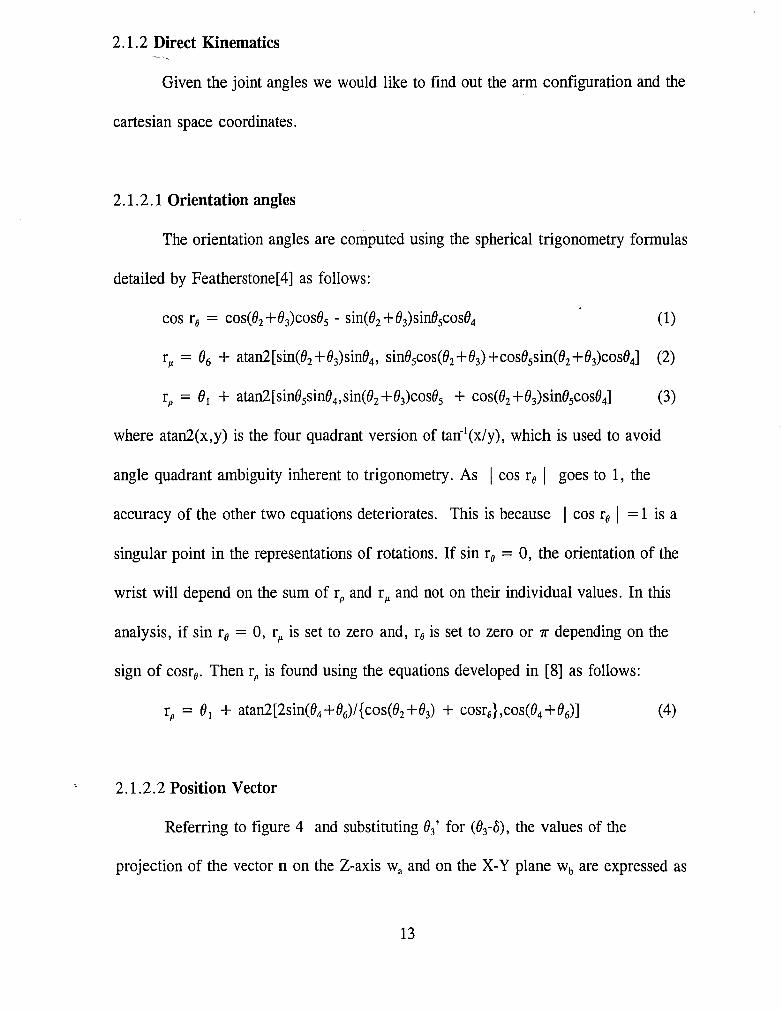
2.1.2.1 Orientation angles

The orientation angles are computed using the spherical trigonometry formulas

detailed by Featherstone[4] as follows:

(1)

rJL = ()6 + atan2[sin(()2 + ()3)sin()4' sin()scos(()2 +()3) +cos()SSin(()2 + ()3)COS()4] (2)

rp = ()1 + atan2[sin()ssin()4,sin(()2 + ()3)COS()S + COS(()2 + ()3)sin()scos()4] (3)

where atan2(x,y) is the four quadrant version of tan-1(x/y) , which is used to avoid

angle quadrant ambiguity inherent to trigonometry. As I cos rei goes to 1, the

accuracy of the other two equations deteriorates. This is because I cos re I = 1 is a

singular point in the representations of rotations. If sin re = 0, the orientation of the

wrist will depend on the sum of rp and rJL and not on their individual values. In this

analysis, if sin re = 0, rJL is set to zero and, re is set to zero or 7r depending on the

sign of cosre. Then rp is found using the equations developed in [8] as follows:

rp = ()1 + atan2[2sin(()4+()6)/{cos(()2+()3) + cosre},cos(()4+()6)] (4)

2.1.2.2 Position Vector

Referring to figure 4 and substituting ()3' for (()3-0), the values of the

projection of the vector n on the Z-axis Wa and on the X-Y plane wb are expressed as

13

Wa = l2cos02 + l3cos(02+03')

Wb = l2sin02 + l3sin(02+03')

Since wbmakes an angle 01 with the Y-axis, the vectors n, WI' w2 can be written as

n = -wbsinOli + WbCOSOlj + wak

w2 = (nx + d2cosOI)i + (ny + d2sin(1)k + wak

WI = (-wbsinOcdcos81)i + (wbcos81-dsin81)j + (wa+ll)k

where d is substituted for dl-d2. Since the vector 14representing the link 14 is

14 = -14sinrosinrpi + l4sinrocosrJ + l4cosrok,

the desired vector r is obtained by adding

rx = -wbsin81 - dcos81- l4sinrosinrp

ry = wbcos81- dsin81 + l4sinrocosrp'

rz = Wa + II + l4cosro·

(5)

(6)

(7)

2.1.2.3 Arm Configuration Parameters

The value of k1 depends on the arm being right or left. If the arm is a lefty,

the projection of the arm on the X-Y plane, Wb, is positive, and vice versa for a right

ann. Thus, to find kl the expression for Wbmust be evaluated. If Wb > = 0, then the

ann is a lefty and kl = + 1. If wb<0, then the arm is a righty and kl = -1.

The value of k2depends on the elbow position. Table I shows four different

combinations that might exist between kl and 83, It is concluded that if kl83> =0,

then the elbow is up and k2 = + 1. If kl83<0, then the elbow is down and k2 = -1.

14

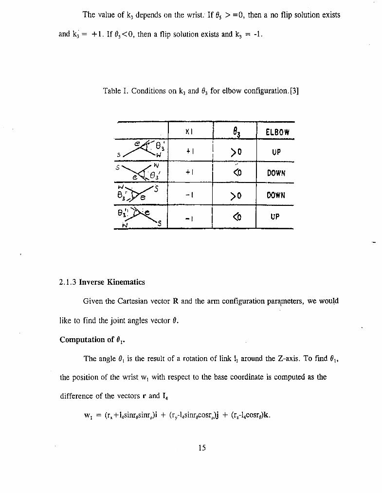
The value of k3 depends on the wrist. If ()s > =0, then a no flip solution exists

and k~ = +1. If 05<0, then a tlip solution exists and k3 = -1.

Table I. Conditions on k3 and 03 for elbow configuration. [3]

KI 83 ELBOW

~8'I

. ! +1 I )0 UPs w I

-S~I\I I .'

e ~eJI +1 <0 DOWN

~~S -I )0 DOWN3/ e

e~ I <0 UP1· -IN S

2.1.3 Inverse Kinematics

Given the Cartesian vector R and the arm configuration para,meters, we wou\d

like to find the joint angles vector o.

Computation of 01"

The angle 8\ is the result of a rotation of link 1\ around the Z-axis. To find 8\,

the position of the wrist w\ with respect to the base coordinate is computed as the

difference of the vectors rand 14

15

To obtain a closed form solution for 81, consider the projection 1of the arm on the X-

Y plane as shown in the figure 4. The projection of 12 and 13 on the X-V plane is

denoted as 12' and 13', respectively. Note that W b is equal in magnitude to 1. From

figure 4b and figure 4c, 81 is calculated as

_--:::~o}tC---.J-_-_-i.o_-----....y

x(a)

xLeft orm8,290--1( 1- t( 2

(b)

Rioht arm

8. • 90-- • I + .c 2

(c)x

Figure 4. (a) Projection of the first three links on the X-Y plane. (b) Calculation of 81

for the left arm. (c) Calculation of 81 for the right arm.[3]

16

81 = 90 - al - kla2

where

al = atan2(klwly , -klwlx)

a2 = atan2(d,I), 0 <a2< 90

and

1 = (w2xy - d2)1I2.

Thus, 81 can be expressed as

81 = atan2(-kIWlx,kIWly) - klatan2(d,I). (8)

Equation(8) indicates that a singular point exists if wlx=wly=O. However, considering

arm geometry, this condition is never satisfied.

Computation of ()2 and ()3

To find angles 82 and 03' consider figure 5 which represents links 12 and 13, the

offset d2, and the different angles used in the computation of O2 and 03' By the

application of the cosine rule to s-e-w'

cos03' = (n2 - 122 - t23)121213 (9)

If I cos03' I > 1 then the position is unobtainable, and if I cos03' I = 1, the

manipulator is at a dead point.

Table II gives the different possible arm configurations for the first three links

and the sign of the different angles. From the table, it is evident that for any arm

configuration

17

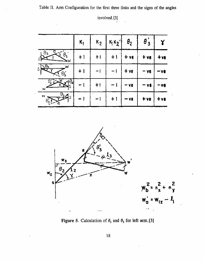
Table II. Arm Configuration for the first three links and the signs of the angles

involved. [3]

.~e2.e -('e I

I Y 3S W

+1 t I +i + ve +ve +VI

-I -I +ve

+I - I - VI

- VI -VI

- ve -ve

W ..~l. (''Ii v

8~., e-I -I +I - VI +VI +VI

222;lib : "x + "y

W~ =W'l - J,

Figure 5. Calculation of 82 and 83 for left ann, [3]

18

(10)

Also,

(11)

where

'Y = klk2atan2(l3sin03',12+13cos03')·

Computation of ()4' ()s and ()6

To find these angles, Featherstone's equations[4] can be applied directly.

(}s = cos((}2+(}3)cosre+sin(02+03)sinrecos(rp-(}I) (12)

If I cos(}s I is not equal to 1, sinOs is computed as (1-cOS2(}s)1I2. If sin(}s > E, where E

is some small number, (}4 and 06 are found from

(}4 =atan2[sinresin(rp-(}I),COS(02 +03)sinrecos(rp-(}I)-sin((}2 +03)cosre] (13)

(}6 = r,,-B (14)

where

B = atan2[sin((}2 +03)sin(rp-(}I),sinrecos(02 + (}3)-cosresin(02 + (}3)cos(rp-(}I)]

The manipulator loses a degree of freedom whenever two joint axes become colinear.

This is the case when sinOs=O and consequently 04 and (}6 become linearly

dependent[4] .

The accuracy of 04 and B deteriorate as sinOs ~ 0, and they break down

completely if sin(}s=O. Therefore, for some value of E and for I sin(}s I < E, better

correspondence can be obtained between (}4 and B by using the equation

(15)

19

In case of a no-flip condition, that is k3 = 1, the wrist angles are obtained from the

above equations. If however, k3 = -1, the flip solution becomes (04+71", -°5, 06+71").

20

3 The Algorithm

3.1 Cartesian Path Approximation

In this chapter three procedures are proposed for selecting intermediate knot

points along an arbitrary smooth cartesian path. The transformation of these points

from cartesian to joint space is also dealt with.

Let the position path of an arbitrary smooth path be represented by P(t), where

pet) is a 3 x 1 position vector. The curvature k(t) can be calculated as follows [2] .

.. • r, _. ..# . •k(t) = «P'P)(p'P)_(p'P)2)112 / (p'P)3/2

where the dot denotes the inner vector product or dot product. The curvatures

corresponding to adjacent points on a smooth path differ only slightly. If the

(16)

difference in curvatures is less than a prescribed tolerance, then the path between the

two points can be considered to be approximately 6ircular with a constant curvature.I(

A path segment is then obtained between two points with approximately the same

curvature. Based on the position trajectory of the given cartesian path, the path

segments are successively determined. The orientation along the path is also known

and can be paramterized by '1.' The orientation corresponding to the two endpoints is

obtained, after the path segment has been determined.

The second procedure uses concatenated line segments to approximate each

path segment obtained from the previous procedure. Since each path segment is

considered to be approximately circular, the problem is reduced to approximating a

21

circle by a polygon. The ratio of the area between the circle and an N sided polygon

should ideally be 1. But since the polygon is only an approximation of the circle,

figure 6. The approximate error area between a polygon and a circle. [3]

(dotted line represents a non optimal side)

22

there is an error in this ratio and this error is specified to be less than a specified

tolerance E. The relationship between Nand E is

27l"(1-E) = Nsin(27l"/N) (17)

For a given E, the smallest N that satisfies (17) is designated as N*. Let the angle

between the line tangent to the circle at one vertex of the polygon and the polygon

side be denoted as 0 (see figure 6). Then 0 is approximately equal to 7l"/N. Let 0* be

denoted by 7l"/N*, where 0* can be considered as a reference index to decide whether

the approximation meets the specified tolerance or not. Consider the approximation of

a path by concatenated line segments. If the angle 0 between the tangent line at one

point on the path and the line segment extending from that point is larger than the

reference angle 0*, then the line segment is not the desired one (see figure 6). An

iterative procedure is carried out until a line segment which has a 0 smaller than 0* is

found. The position and orientation corresponding to the two endpoints of the line,

are saved. This procedure is repeated until all the path segments are approximated by. ~i

line segments. Note that the endpoints of all line segments lie on the cartesian path

itself.

Once the concatenated line segments are determined, the next step is to

determine intermediate knot points which are subsequently transformed to joint space.

The procedure is similar to the one used in [9] where the positions and orientations

corresponding to the endpoints of the line segments are utilized. The endpoints of a

23

line segment are transformed to joint space. The mid point between these two points

in joint space is determined and transformed back to cartesian space. This transformed

point is compared with the mid point of the line segment calculated from the cartesian

space endpoints. The deviation between these two points in position and orientation

should be within a prescribed tolerance. If not, the mid point in cartesian space is

chosen as the end point of the same line segment and the procedure is repeated until

the deviations are within specified bounds. Once an intermediate knot point has been

selected, this procedure is repeated between the knot point and the original endpoint

until a series of intermediate knot points is selected for a single line segment. This

procedure is then repeated for successive line segments, finally resulting in a series of

knot points describing the cartesian path.

The knot points must now be transformed to joint space. For this purpose, the

equations developed in [3] were utilized. The solution is based on a method that fully

exploits the special geometry of the PUMA 560 robot. Special attention is .,given to

the arm configuration in both directions. The algorithm presented here is an

adaptation of the one presented in [2].

3.2 Divide a Cartesian Path into Path Segments.

The motion of the end effector in cartesian space is expressed as

H = [ Px' Py , Pz' Px' Py ' Pz F = [pT, TTF

where

pT = [Px,Py. PJ is the position vector,

24

RT = [Px' Py, pJ is the orientation vector.

The angles Px, Py, Pz are the rotational angles about the Z-axis, the new X-axis and

the new Z-axis respectively, that align the manipulator base coordinates with the end

effector coordinates.

The algorithm to divide the cartesian path into segments is as follows:

1) Let Ts be the starting time and Tg..be the ending time of the cartesian path.

Let i denote the subscript for the ith path segment. Assign To = Ts and Tf =

To.( Start at the beginning of the path)

2) Compute 0t = (Tg - Ts)/df where df usually is 2. Thus 0t is an increment in

time. Compute Tf = To + nOt where n starts from O. 'n' denotes the number

of time increments advanced.

Check whether Ik(To) - k(Tt) I > ~1 (18)

where k(T) is the curvature of the path at time T and is expressed using

equation (16).

If (18) is not true, n = n+1 until (18) is satisfied.

If Tf > = Tg then set Tf = Tg and end this procedure. Otherwise, go to the

next step.

In this step we are trying to find a range of time in which the curvature of the path is

approximately constant. We move forward in time starting with Tf = To. Thus, for

25

example the above condition may be satisfied when Tf is To + 30t • In this case the

actual value of Tf when the difference in curvatures exceeds ~ 1 is somewhere between

To + 2(\ and To + 30t •

3) Now let 0/ = o/df. Let m = 0;

Tf = Tf - mot' (19)

check whether I k(To)-k(Tf) I < ~1 (20)

If (20) not true, m = m+1 and repeat eqns (19) and (20) until the above

condition is satisfied.

The algorithm as stated above and in [2] will not work in this case because equation

(20) will eventually give a negative value for Tf when equations (20) and (21) are

repeated. In order to overcome this problem, let Tf' = Tf - mo/ and check whether

I k(To)-k(Tf') I < ~1' Increment m until the condition is satisfied. If Tf' equals To

then let Tf' be equal to the original Tf. Now we are moving back in time in steps of

0t' in order to determine the path segment whose curvature is approximately constant.

4) Save the endpoints of the segment. Hi = R(Tf'). The endpoints of the

segment in time are now Tsi = To and Tgi = Tf'. Let To = Tf' and repeat

steps 2, 3 and 4.

5) End of procedure.

26

3.3 Approximating Path Segments with Line segments

In the previous procedure the cartesian path was split into segments so that

each segment can be considered as a circular arc. In this procedure these path

segments are approximated by line segments. The procedure for approximating a path

segment with straight line segments is as follows:

1) Let To = Tsi and Tf = Tgi starting with i = 0;

The unit tangent vector T(To) at H(To) is given by

T(To) = P(To)/ I I P(To) I I = [tx(To), ty(To), ~(To)F

where the operator I I I I I denotes the magnitude of the vector I.

2) The unit vector from H(To) to H(Tf) is given by

L(To,Tf) = (P(Tf)-P(To»/ I I P(Tf)-P(To) I I

Let L(To,Tf) = [1/To,Tf), l/To,Tf), lzCTo,Tf)]T

The angle between the tangent vector and the unit line vector is given by

8 = ATAN2(1-(txlx + tyly + ~IJ, txlx + tyly + ~lz )

This formula, given in [2] is incorrect. The correct formula is

8 = ACOS(1-(txlx + tyly + ~IJ, txlx + tyly + ~lz )

From the first procedure the path segments of same curvature were found. As

explained previously, approximating the path segments by line segments is done by

first considering the approximation of a circle by an N sided polygon. The condition

27

to be fulfilled here is that the ratio of the area of the polygon to that of the circle.<::

should be less than or equal to a specified tolerance ~2' Thus we get

For a given ~2 the smallest integer N that satisfies this equation is designated as N*.

The angle between the tangent line at one vertex of the polygon and the corresponding

polygon side is given by ?fIN. Thus e* = ?f/N*. This can be considered as the

optimum angle. If the e that is calculated is greater than eo, then N is not the

required number of line segments and the iterative procedure that follows is used for

calculating N.

3) Check whether I e* - e I < ~2

If this is not satisfied, then let Tf = (To +Tf)/df and go to the previous step 2.

Thus, we go back in time until we obtain a line segment that approximates that part

of th~ cartesian path between To and Tf.

4) Save the endpoints of the line segments, i.e. H/Tf). Let To = Tf, Tf =

Tgi and increment j by using j = j + 1. Repeat these four steps until To =

Tgi. Then do the same procedure for the next path segment and so on.

28

( 3.4 Generation of Intermediate Knot Points.

In general, when a curve is to be approximated by straight lines, it is desirable

to sample as many points as possible on the curve. But since this is computationally

ineffecient, points on the curve are selected based on approximations. This procedure

describes the selecting of intermediate knot points on the cartesian path segment.

1) Consider the first line segment of the first path segment, or generally

speaking the jth line segment of the ith path segment.

Let Hij = H1eft and H jj+1 = Hright

2) Find the joint vectors corresponding to the above two positions. Let these

be called J1eft and J right

In transforming coordinates from cartesian space to joint space we make use of the

equations given in [3] and [4]. These equations have been specially developed for the

PUMA 560 taking into account the specific geometry and possible configurations for

a single coordinate. The derivation of these equations is explained in [4] and these

have been modified to specially suit the PUMA 560 in [3].

Compute the mid point in joint space by

29

Now the corresponding transformation to cartesian space is done by forward

k' , J ., H - [pT R T]Tmematlcs on mid glvmg mid - mid' mid '

Also, compute the mid point in cartesian space

4) The deviations between the mid point calculated from the cartesian space

coordinates and the mid point in cartesian space computed by the forward

kinematics of the mid point in joint space are calculated as

Op = E I p mid - pcenter I

Or = E I Rmid - Reenter I

5) Check whether op < Op max and Or < Or max' where op max and Or max have been

previously specified by the user. If these conditions are not satisfied, then let

H right = Hcenter and repeat the steps 2 to 4, until the conditions are satisfied, i.e.

move back in space along the line segment until a point can be selected so

that that segment in joint space is a reasonable approximation of the

corresponding line segment. If the conditions are never satisfied, then take the

mid point of the original line segment as a knot point and move on to the next

line segment. Let H 1cft = Hright and Hright = H gOa1 where H goal = H ij + 1• This

procedure is repeated for each and every line segment, resulting in a series of

points in joint space which have to be splined.

30

3.5 Splining of Knot Points.

As a result of the previous procedures, a series of knot points in joint space

has been obtained. As explained previously, when these points are tranformed back to

cartesian space they will approximate the given cartesian path within specified error

bounds. In order to obtain a continuous trajectory in joint space, these knot points

must be splined. The procedure for splirring developed in [2] is explained first. This is

followed by. an explanation of the procedure developed by the author in the next

chapter.

Let the knot points in space be arranged as y(fo), y(tl) ...y(~), where y(to)

denotes the knot point 'y' at time to. A fourth order polynomial Qlt) can be

represented as

(21)

where Qlt) is the spline joining the points yeti) and y(t j + l) and is parameterized by the

time variable t E [t j , 4+a and i = 0, 1,2, ... , n-l. The path continuity constraints are

Further, for local smoothness it is required that

ti +1

J[Qi(t)fdt be minimized.tt

Based on the above criterion recursive formulas for calculating the coeffecients in the

above equation are as follows.

31

ei = Yi

di = 4ai_1h\1 + 3bi_1h\1 + 2Ci_1hi_1 +di_1

Ci = 6ai_1h\1 + 3bi_1hi_1 + Ci_1

bi = (9/4)(Yi+l - y)h-3i - (9/4)~h-Zi - (1l/6)cih-1j

ai = -(5/4)(Yi+l - Yi)h-4i + (5/4)dih-3i + (5/6)cih-Z

(22)

(23)

(24)

(25)

(26)

where hi = ti+1- ti for i = 2,3, ... ,n-3. The variable 'h' is used to denote the

difference in time between two knot points. The knot points used in these equations

are Yi and Yi+l where Yi represents yet). This is done for the sake of legibility.

The initial values for the equations (22-26) are Cz and dz. Let tracking error be

defined as

TEi = titi +1J[Qi(t) - Li(t)F dt

where Llt) = desired path between Yi and Yi+l and is given by

Li(t) = Yi + (Yi+l - Yi)(ti+1- ~ tf(t-~)

The total tracking error is E TEb i = 2 to n-3.

To simplify computation, Cz is taken as constant. Thus, this becomes a single variable

optimization problem. aTEIadz yields

dz* = (YrYz)h-1 +(kz/k1)czhz

where kz = 2416 and k1 = -1057.2

In other words dz can be taken to be the user specified initial velocity, and Cz can be

the user specified acceleration. The final segments must satisfy the following

constraints:

32

. ..Qn-2(~-) = Qn-l(~l)

.. ..Qn-2(tn-1) = Qn-l(~l)

•Qn-2(tn-l) = Wn-2

..

where Wn-2' Wn-l' a n-2 and an are the desired accelerations and velocities.

Since there are more equations than unknowns, the solutions will not be

unique. Hence a pseudo knot point is added. This point is chosen so that the tracking

error in the final segments is minimized. The values of the coeffecients for the pseudo

point are found from

MrXr = Nr

where

h4 h3 0 0 0 0 -1

4h3 3h2 0 0 0 -1 0

12h2 6h 0 0 -2 0 0

Mr = 0 0 h4 h3 h2 h 1 (27)

0 0 4h3 3h2 2h 1 0

0 0 12h2 6h 2 0 0

15h4 17h3 h4/5 h3/4 h2/3 h/2 37956 72 252

33

IJ

an_zbn_zan_1

bn_1

Cn-Id

n_1

en-I

en_z - dn_zh -cn-zhZl- dn-z -cn_zh-2cn_zenWn

an

rJn

where rJn = (719/1260)en_z +(14/15)en +(7/36)cn_zh2 +(173/1260)dn_zh

and h = (l12)(fn - fn-2)

In this case the end velocity and acceleration are user specified.

(28)

(29)

The pseudo knot YI is likewise added at the beginning. The coeffecients for this are

found from

aobo

X s = al

bl

CI

dl

e l

eo - doh -cob2

- do -cob-2co

Ns = ezWz

az1]0

34

(30)

(31)

h = (112)(~ - ~)

Tlo = (719/1260)eo +(14/15)ez +(7/36)cohZ +(l73/1260)dah

Now the coordinates of a single joint have been spUned. This procedure is repeated

for all the other joints.

35

4 Proposed Algorithms

4.1 Proposed Procedure.

Two methods are proposed in the following sections. The same smoothness

criterion is used in developing the recursive equations to calculate the spline

coeffecients. In this case the starting values for the system of equations are co, do and

eo, the initial acceleration, velocity and position of the end effector, respectively.

Substituting these in the recursive equations for t = to to tn-1 will give us the values of

the spline coeffecients, but the final values of acceleration and velocity will be

determined by the equations and not by the user. In order to allow the user to specify

,a final velocitY and acceleration, the following is procedure is adopted.

4. 1.1 Procedure 1

At time ~-2 the values of cn_2, dn_2, en-2 are known. Instead of using these values

to find an-2 and bn-2 in the recursive equations, let an-2, the fourth order coeffecient in

the spline Qn-2 be denoted as an-2 itself. As explained previously, if the recursive

equations are used to compute all the coeffecients, the end velocity and acceleration

becomes determined by the system of equations itself and not by the user.

Substitute for bn-2 in terms of an-2 in the equation for the spline Qn-2 at time ~-l'

where

h = ~-l - ~-2

36

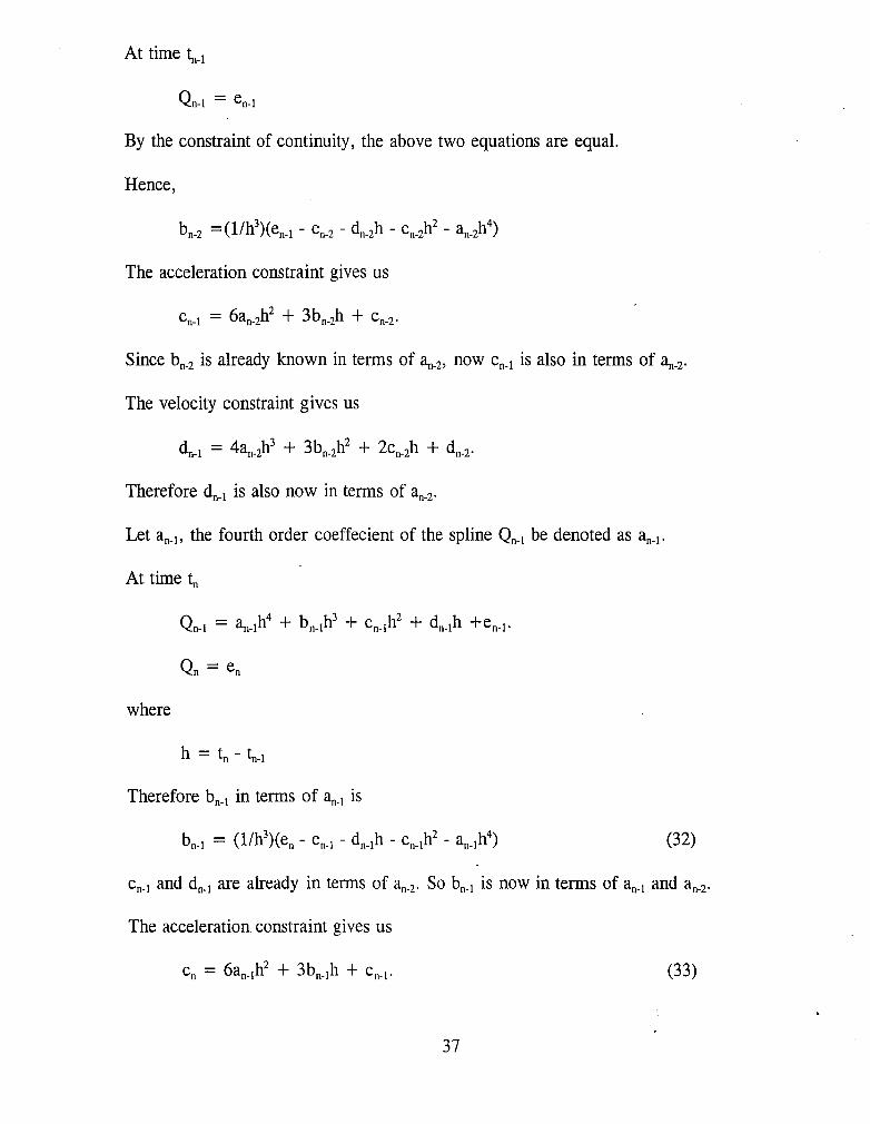
At time 1:n-1

By the constraint of continuity, the above two equations are equal.

Hence,

bn-2 = (lIh3)(en_1 - en-2 - dn_2h - cn_2h2

- an_2h4

)

The acceleration constraint gives us

cn-l = 6an_2h2 + 3bn_2h + cn-2 ·

Since bn_2 is already known in terms of ~-2' now Cn-l is also in terms of ~-2'

The velocity constraint gives us

dn-l = 4an_2h3 + 3bn_2h

2 + 2cn_2h + dn-2•

Therefore dn-l is also now in terms of an-2•

Let an-I' the fourth order coeffecient of the spline Qn-l be denoted as ~-l'

At time 1:n

Qn-l = an_lh4 + bn_lh

3 + cn_lh2 + dn_lh +en-l·

Qn = en

where

h = ~ - 1:n-1

Therefore bn_l in terms of an-l is

bn-l = (lIh3)(en- enol - dn_lh - cn_lh2

- an_lh4) (32)

cn-l and dn_l are already in terms of an_2. So bn-l is now in terms of ~-l and an-2•

The acceleration constraint gives us

(33)

37

Since bn_, is already~known in terms of an_I and an-2, now Cnis also in terms of an_I and

an-2. The velocity constraint gives us

(34)

Therefore dnis also now in terms of an-I and an-2. The final acceleration and velocity

are Cnand dn, respectively. They are now user specified. Once Cnand dnare specified,

equations (33) and (34) can be solved for an-I and an-2. From these values the rest of

the coeffecients can be found since they are in terms of ~_I and an-2.

4.1.2 Procedure 2

In this procedure the recursive equations are used instead of the equation of

the spline itself, to find the coeffecients of all the splines. Two pseudo knot points are

added to the original set of points. The first pseudo knot is added between the knot

points n-2 and n-l and is assumed to be at time

t' = tn_2 +((In-I - In_2)/2).

Let the coeffecients of the spline at the first pseudo knot be a', b', c', d', e'. Let the

coeffecients at the second pseudo point be a", b", c", d", e". The second pseudo

point is added between the knot points at n-l and n at time

t" = tn_I + ((In - ~_I)I2)·

At time In-2' Cn_2and dn-2are known from the recursive equations. In the equation fo~

an-2, substitute y' instead of Yi+ I'

an-2 = -(5/4)(y'- y)h-4j + (5/4)~_2h-3n-2 + (5/6)cn_2h-2n_2

bn~2 = (9/4)(y'- Yn_2)lr3n_2- (9/4)~_2h-2n_2- (l1l6)cn_2h-In_2

38

(35)

(36)

where

.,

These values of an-2 and bn-2 are substituted in the equations for c' and d'

e' = y'

Since an-2 and bn-2 are in terms of y', c' and d' are also now in terms of y'.

Substituting these values in the recursive equations we get

a' = -(5/4)(Yn_l- y')h,-4 + (5/4)d'h'-3 + (5/6)c'h'-2

b' = (9/4)(Yn_c y')h'-3 - (9/4)d'h'-2 - (1l/6)c'h,-1

c = 6a'h,2 + 3b'h' + c'n-I

d = 4a'h,3 + 3b'h,2 + 2c'h' +d'n-I

en-I = Yn-I

where

h' = ~_I - t'

cn_1 and dn_1are now in terms of y'.

e" = Y"

39

(37)

(38)

(39)

(40)

(41)

(42)

(43)

(44)

(45)

(46)

(47)

(48)

(49)

where

hn_1 = t" - ~_I' (50)

Since Cn_1 and dn_1are in tenns of y', ~_I and bn_1 are in tenns of y" and y'. Thus c"

and d" are also- now in tenns of y' and y". Substituting these values in the recursive

equations again we get

a" = -(5/4)(Yn- y")h"-4 + (5/4)d"h"-3 + (5/6)c"h";2

b" = (9/4)(Yn- y")h"-3 - (9/4)d"h"-2 - (1116)c"h,,-1

c = 6a"h"2 + 3b"h" + c"n

d = 4a"h"3 + 3b"h"2 + 2c"hlF- + d"n

where

h" = tn - t".

The final acceleration and velocity are cn and dn' respectively. They are user

(~1)

(52)

(53)

(54)

(55)

specified. Once these are specified, equatons (54) and (55) can be solved for y' and

y". The values of y' and y" so obtained can be substituted back into the equations

above to detennine ~he coeffecients an-2, bn_2, a', b', c', d', e', an_I' bn_l , cn_l , dn-I, en-I,

a", b", c", d", and e". Now that the points have been splined, the paths have to be

tracked.

40

4.2 Path Tracking in Joint Space.. ,

The PUMA 560 is assumed to have a micro stepping motor. Consider a single

joint. The position of the shaft is indicated by sensors. This is compared to the

required position calculated from the corresponding spline equation. The square of the

distance between the two is calculated. A step is taken in the direction that reduces

the square of the'distance between the two positions. The basis for this algorithm was

obtained from [6].

1) Find present position of the shaft from sensors at time t

2) The position of the shaft at time t+ (time it takes for the shaft to move

through a step) is calcu~_ated from the corresponding spline equation.

3) The distance moved is divided by the resolution of the stepper motor in

order to obtain the number of pulses.

4) The position of the shaft +

a) (# of pulses*resolution) in one direction

b) (# of pulses*resolution) in the opposite direction

c) no step

41

is found. The squares of the distance of each of the three cases from the

position calculated in step 2 is found. The option that gives the minimum of

these squares is chosen. This tracking algorithm is applied to the splines for

each joint.

4.3 Parameters of the Model used for the Simulation

A simulation was performed in order to test the proposed procedures. The

simulation program was written in e and executed on an IBM RISe 6000

workstation. The cartesian path, configuration of the PUMA 560 and stepper motor

parameters that were used in the simulation are given in the following sections.

4.3.1 Cartesian path

The end effector of the robot is to follow a cartesian path that is parameterized

by the time variable 't' and is defined by

H(t) = [Px(t), Pit), Pz(t), px(t), pit), pzCt)F

where

Pit) = 8(t) - sinO(t), Py(t) = I - cos8(t), Pz(t) = 0

px(t) = 7r/2 - m/4, pit) = 'Tr/2, pz(t) = 7r/2

8(t) = 2m and 0.01 < t ~ 1.

The starting and ending positions in terms of base coordinates are given, respectively,

as

H(Ts) = [40,400,600,90 0 ,90 0 ,90°F

42

4.3.2 Arm Configuration parameters

As explained previously in section 2.1.1.1, the robot arm may be lefty or

righty, i.e. it may resemble a human's left arm or right arm, respectively. The elbow

can have two configurations. When the elbow's position is above the line joining the

shoulder and the wrist, the elbow is up. When the position of the elbow is below that

line, the elbow is down. The wrist also has two configurations. A no-flip wrist where

the joint angle Os is positive, and a flip wrist for which Os is negative. The

configuration paramenter for the arm, elbow and wrist of the robot are denoted by k[,

k2 and k3, respectively. Table III gives the values of these parameters used in the

simulation.

Table III. Arm Configuration Parameters

Arm Elbow Wrist

k[ = -1 k2 = +1 k3 = -1

righty up flip

43

4.3.3 Stepper motor parameters

The PUMA 560 is equipped with a DC servomotor which receives feedback in

the form of pulses from a digital encoder. In this study, it is assumed that the PUMA

560 is equipped with a stepper motor whose details are given in Table IV. This is a

simplifying assumption. The algorithm can be applied to feedback from digital

encoders for joints that are driven by sevo motors.

Table IV. Stepper motor parameters

steps per revolution 400

speed (rps) 50

acceleration range (deg/sec/sec) 0-999

.".,...

Maximum pulse rate (kHz) 20

4.4 Analysis of the results

Efficient algorithms for the approximation of cartesian space trajectories and

trajectory tracking have heF~developed and presented here. These algorithms are

based on the methods developed by [2] and [6]. A comparison between the algorithm

presented by Chang et al [2] and the one in this study gave the following results.

44

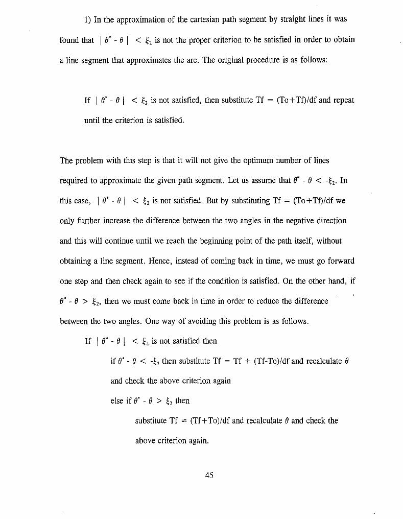
1) In the approximation of the cartesian path segment by straight lines it was

found that I e* - eI < ~2 is not the proper criterion to be satisfied in order to obtain

a line segment that approximates the arc. The original procedure is as follows:

If I e* - eI < ~2 is not satisfied, then substitute Tf = (To + Tf)/df and repeat

until the criterion is satisfied.

The problem with this step is that it will not give the optimum number of lines

required to approximate the given path segment. Let us assume that e* - e < -~2' In

this case, I e* - eI < ~2 is not satisfied. But by substituting Tf = (To + Tf)/df we

only further increase the difference between the two angles in the negative direction

and this will continue until we reach the beginning point of the path itself, without

obtaining a line segment. Hence, instead of coming back in time, we must go forward

one step and then check again to see if the condition is satisfied. On the other hand, if

e* - e > ~2' then we must come back in time in order to reduce the difference

between the two angles. One way of avoiding this problem is as follows.

If I e* - eI < b is not satisfied then

if e* - e < -~2 then substitute Tf = Tf + (Tf-To)/df and recalculate e

and check the above criterion again

else if e* - e > ~2 then

substitute Tf = (Tf+To)/df and recalculate eand check the

above criterion again.

45

This procedure gives the correct number of line segments that can be used to

approximate the cartesian path segment. Figure 7b illustrates what could happen if the

original procedure is followed.

2) Chang's[2] algorithm requires eight inputs to the manipulator in the splining

phase. The inputs are the velocities and accelerations at the start point, the second

point, the next to the last point and the end point. Both procedures presented here

require only four inputs: The velocities and accelerations at the beginning and end

points, which is the normal practice.

3) By introducing a pseudo knot at the beginning of the spline, any error

associated with that point will be propogated throughout the whole trajectory. That

problem is avoided here by introducing both pseudo knots at the end.

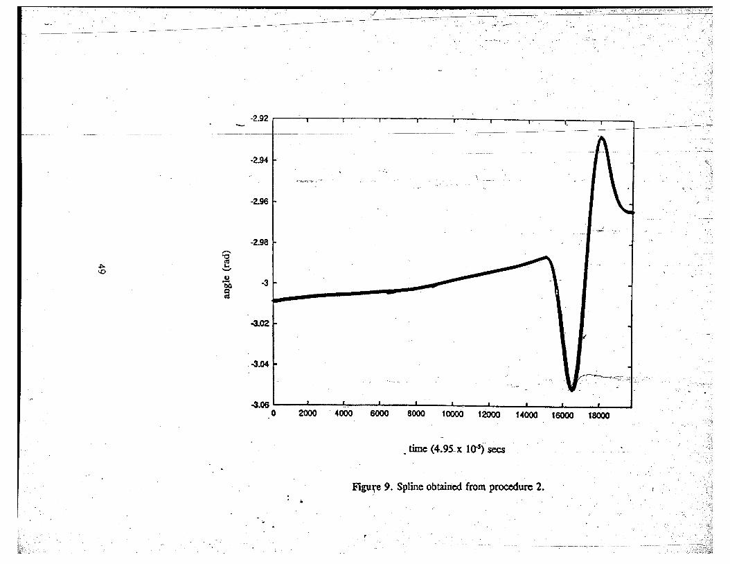
4) The splining method presented here is computationally simple compared to

Chang's algorithm. The splines obtained from both procedures for Joint 1 are shown

in figure 8 and figure 9.

5) A comparison of figure 8 and figure 9 shows that the spline obtained as a

result of procedure 2 which utilized the local smoothness constraint while calculating

the coeffecients of the last two splines, is not as smooth as the spline obtained from

procedure 1 which did not utilize that constraint. This would indicate that procedure 1

performs better than procedure 2. However, not enough examples were performed to

draw this general conclusion. Neither one has been proven to be better than the other.

In fact, both are based on similar procedures.

46

figure 7. (a) Optimum angle greater than calculated angle. (b) Optimum angle lesser

than calculated angle.

47

'-

.. 1

'"

_~-=s-~.=-.,(~. -. .~

figure 8. 'Spline obtained from procedure 1.

2000 "000. 6000 8000 10000 12000 14000 16000 18000

time (4.9Sx lo-s) sees

":~~:"'.~-.... ~- :

-2.92 I I I I I I I ,- I I ,

-2.94

..-=~:.:-~~.-;;- :

-2.96 r

"".~

-2.98

~'-0

,-..e'-"I)

} -3 L u.-

-3.02

.-3.04, ........:;.

-3.06' , '_ ' • I , , , , Io 2000 4000 6000 8000 10000 12000 104000 16000 18000

• time (4~95-x lOoS) sees-

Figu~ 9. Spline obtained from procedure 2...

5 Conclusions

5.1 Conclusions

Efficient algorithms for the planning of cartesian trajectories and subsequent

tracking in joint space have been developed. The work done in [2] and [6] fo~s the

basis for these algorithms. A procedure for selecting knot points in cartesian space

based on the curvature of the cartesian trajectory was first developed. These points

were then transformed to joint space using kinematic transformations developed

specially for the PUMA 560. The points in joint space were then splined using two

methods. The transformation of this spline from joint space to cartesian space, results

in a trajectory that closely approximates the cartesian trajectory initially specified.

The algorithm in [2] has been suitably modified to give correct results. An attempt

was made to simulate the algorithm in [2], but was unsuccessful. A program was

written to simulate the algorithm in [2] but, the expected results were not obtained.

The procedures proposed for splining of knot points in joint space are simple and do

not involve complex computations. The kinematic equations used for the PUMA are

also efficient and exploit the simple geometry of the arm.

The solution approach develops a good physical understanding of the

manipulator and provides geometric insight into the transformation problem and also

helps one to understand the difficulties involved in trajectory planning.

A comparison between the algorithms developed here and the algorithms

presented in [2] gives the following results:

50

1) The criterion presented in [2] which is used to determine the number of line

segments required to approximate the cartesian path is inadequate. The proper

criterion to be used can be found in the discussion of the results.

2) The proposed splining procedures require fewer inputs than the procedure in [2].

3) The error introduced when adding a pseudo knot point at the beginning of the

trajectory, which propogates throughout the splining procedure is reduced by

introducing the pseudo knot point at the end.

4) The proposed splining methods are computationally simpler.

5) The procedure which did not incorporate the local smoothness criterion seems to

perform better than the procedure which incorporates the smoothness criterion. But

further tests must be performed before a general statement can be made.

5.2 Directions for Future Research

The algorithms presented here are derived assuming the manipulator to be a

rigid body. Lightweight manipulator design reduces driving torques for high speed

and heavy payload manipulators. However, during such operations, the manipulator is

likely to deform, thereby reducing accuracy and creating stability problems. Chang

and Hamilton [1], derived the kinematics of a flexible manipulator using an

Equivalept Rigid Link System (ERLS) model. The ERLS is a hypothetical system

whose motion and kinematics resemble that of a rigid link system.The global motion

of the flexible manipulator is thus split into a large motion representing the ERLS and

a superimposed small motion which is due to the deviations with respect to the ERLS.

51

Kinematic equations in terms of the Hartenberg-Denavit matrix have been developed

and take into account the deviations due to the flexibility of the manipulator.

These equations could be incorporated into the algorithm presented here in order to

make it applicable to flexible manipulators.

-.....Another consideration is the modification of the forward kinematic equations in

the neighborhood of singularities. As has been reported, the accuracy of some of the

other kinematic equations deteriorates in the neighborhood of a singular point. Lai and

Yang[5] have proposed a scheduling method to overcome this problem.

Finally, another consideration for future research is the control of manipulator

trajectory. Various schemes have been proposed, and most of them work

satisfactorily. The problem is to obtain a procedure that is not computationally

complex, while at the same time giving satisfactory results.

52

References

[2] Chang, Yeong-Hwa, Lee, Tsu Tian and Liu, Chang-Huan, "On-Line Approximate

Cartesian Path Trajectory Planning for Robot Manipulators," IEEE Transactions on

Systems, Man and Cybernetics, vol. 22, no.3, pp. 542-547, May/June 1992.

[3] Elgazaar, Shadia, "Effecient Kinematic Transformations for the PUMA 560

Robot," IEEE Journal of Robotics and Automation, vol. RA-l, no.3, pp. 142-151,

September 1985.

[4] Featherstone, R., "Position and Velocity Transformations Between Robot End­

Effector Coordinates and Joint Angles," International Journal of Robotics Research,

vol.2, no.2, pp. 34-45, Summer 1983.

[5] Lai, Jim Z.C., and Yang, Daniel, "An Effecient Motion Control Algorithm For

Robots with Wrist Singularities," IEEE Transactions on Robotics and Automation,

vol.6, no.l, pp. 113-117, February 1990.

53

[6] Lianos, T., Kiritsis, D., and Aspragathos, N., "A Direct Algorithm for

Continuous Path Control," Robotics and Computer Integrated Manufacturing, vol.8,

no.2, pp. 97-101, 1991.

[7] Lin, C.-S., Chang, P.-R., and Luh, J.Y.S., "Formulization of Optimization of

Cubic Polynomial Trajectories for Industrial Robots," IEEE Transactions on

Automation and Control, vol. AC-28, no.12, pp. 1066-1074, December 1983.

[8] Luh, J.Y.S., and Lin, C.-S., "Approximate Joint Trajectories for Control of

Industrial Robots along Cartesian Paths," IEEE Transactions on Systems, Man, and

Cybernetics, vol SMC-14, pp. 444-450, May/June 1984.

[9] Paul, R.P., "Manipulator Cartesian Path Control," IEEE Transactions on Systems,

Man and Cybernetics, vol. SMC-9, pp. 702-711, November 1979.

[10] Taylor, R.H., "Planning and Executing of Straight Line Manipulator

Trajectories," IBM Journal of Research and Development, vol.23, noA, pp. 424­

436, July 1979.

54

Name:

Date of Birth:

Current Address:

Vita

Dwaraka Srinivasan.

6 / 10 / 71

422 Pierce Street, 2nd Floor, BetWehem,PA 18015.

Permanent Address: 9127 Edmonston Court, Apt. No. 203,Springhill Lake Apartments, Greenbelt,MD 20770.

Education: Bachelor of Engineering, MehanicalEngineering, Coimbatore Institute ofTechnology, India, 1992.Master of Science, Industrial Engineering,Lehigh University, 1994.

55