algorithms in data mining using matrix and tensor...
TRANSCRIPT

ii
�phdBerkant� � 2008/4/28 � 10:32 � page i � #1 ii
ii
ii
Linköping Studies in Science and TechnologyDissertations, No 1178
Algorithms in
Data Mining using
Matrix and Tensor Methods
Berkant Savas
A · (X, Y, Z)
A · (X⊥, Y, Z)
A · (X, Y⊥, Z)
A · (X⊥, Y⊥, Z)
A · (X, Y, Z⊥)
A · (X⊥, Y, Z⊥)
A · (X, Y⊥, Z⊥)
A · (X⊥, Y⊥, Z⊥)
Department of MathematicsScienti�c Computing
Linköping 2008

ii
�phdBerkant� � 2008/4/28 � 10:32 � page ii � #2 ii
ii
ii
Linköping Studies in Science and TechnologyDissertations, No 1178
Algorithms in Data Mining using Matrix and Tensor Methods
Copyright c© 2008 Berkant Savas
Scienti�c Computing
Department of Mathematics
Linköping University
SE�581 83 Linköping, Sweden
[email protected]/Num/
ISBN 978-91-7393-907-2ISSN 0345-7524
The thesis is available for download at Linköping University Electronic Press:http://urn.kb.se/resolve?urn=urn:nbn:se:liu:diva-11597
Printed by LiU-Tryck, Linköping 2008, Sweden

ii
�phdBerkant� � 2008/4/28 � 10:32 � page iii � #3 ii
ii
ii
To Alice, Jessica and my family

ii
�phdBerkant� � 2008/4/28 � 10:32 � page iv � #4 ii
ii
ii

ii
�phdBerkant� � 2008/4/28 � 10:32 � page v � #5 ii
ii
ii
Abstract
In many �elds of science, engineering, and economics large amounts of data arestored and there is a need to analyze these data in order to extract informationfor various purposes. Data mining is a general concept involving di�erent tools forperforming this kind of analysis. The development of mathematical models ande�cient algorithms is of key importance. In this thesis we discuss algorithms forthe reduced rank regression problem and algorithms for the computation of thebest multilinear rank approximation of tensors.The �rst two papers deal with the reduced rank regression problem, which is
encountered in the �eld of state-space subspace system identi�cation. More specif-ically the problem is
minrank(X)=k
det(B −XA)(B −XA)T,
where A and B are given matrices and we want to �nd X under a certain rank con-dition that minimizes the determinant. This problem is not properly stated sinceit involves implicit assumptions on A and B so that (B−XA)(B−XA)T is neversingular. This de�ciency of the determinant minimization is �xed by generalizingthe criterion to rank reduction and volume minimization of the objective matrix.The volume of a matrix is de�ned as the product of its nonzero singular values.We give an algorithm that solves the generalized problem and identify propertiesof the input and output signals causing a singular objective matrix.Classi�cation problems occur in many applications. The task is to determine the
label or class of an unknown object. The third paper concerns with classi�cationof handwritten digits in the context of tensors or multidimensional data arrays.Tensor and multilinear algebra is an area that attracts more and more attentionbecause of the multidimensional structure of the collected data in various applica-tions. Two classi�cation algorithms are given based on the higher order singularvalue decomposition (HOSVD). The main algorithm makes a data reduction usingHOSVD of 98�99 % prior the construction of the class models. The models arecomputed as a set of orthonormal bases spanning the dominant subspaces for thedi�erent classes. An unknown digit is expressed as a linear combination of the ba-sis vectors. The resulting algorithm achieves 5% in classi�cation error with fairlylow amount of computations.
v

ii
�phdBerkant� � 2008/4/28 � 10:32 � page vi � #6 ii
ii
ii
The remaining two papers discuss computational methods for the best multilin-ear rank approximation problem
minB‖A − B‖,
where A is a given tensor and we seek the best low multilinear rank approximationtensor B. This is a generalization of the best low rank matrix approximationproblem. It is well known that for matrices the solution is given by truncating thesingular values in the singular value decomposition (SVD) of the matrix. But fortensors in general the truncated HOSVD does not give an optimal approximation.A third order tensor B ∈ RI×J×K with rank(B) = (r1, r2, r3) can be written asthe product
B = (X,Y, Z) · C, bijk =∑λ,µ,ν
xiλyjµzkνcλµν ,
where C ∈ Rr1×r2×r3 and X ∈ RI×r1 , Y ∈ RJ×r2 , and Z ∈ RK×r3 are matriceswith orthonormal columns. The approximation problem is equivalent to a non-linear optimization problem de�ned on a product of Grassmann manifolds. Weintroduce novel techniques for multilinear algebraic manipulations enabling the-oretical analysis and algorithmic implementation. These techniques are used tosolve the approximation problem using Newton and quasi-Newton methods specif-ically adapted to operate on products of Grassmann manifolds. The presentedalgorithms are suited for small, large and sparse problems and, when appliedto di�cult problems, they clearly outperform alternating least squares methods,which are standard in the �eld.
vi

ii
�phdBerkant� � 2008/4/28 � 10:32 � page vii � #7 ii
ii
ii
Populärvetenskaplig
sammanfattning
Inom många vetenskapliga, tekniska, ekonomiska och internetbaserade områdensamlas och lagras stora mängder data som innehåller värdefull information. Dennainformation är inte direkt tillgänglig utan man behöver analysera data för attkomma åt informationen. Datautvinning (data mining) är ett generellt begreppsom innehåller olika verktyg för att extrahera data och information. Särskilt viktigtär utvecklingen av matematiska modeller, algoritmer samt e�ektiv implementeringav dessa på olika datorsystem. I denna avhandling utvecklar vi teori och algoritmerför datautvinning genom matris- och tensorberäkningar. Teorin och algoritmernaveri�eras genom att tillämpas inom systemidenti�ering och klassi�cering av hand-skrivna si�ror.Målet med systemidenti�ering är att bestämma matematiska modeller av dy-
namiska system, som ett �ygplan eller en bilmotor, baserat på uppmätta in- ochutsignaler. Den beräknade modellen relaterar insignaler till utsignaler. Modellenanvänds sedan i syfte att reglera och simulera systemet. I processen ingår ettminimeringsproblem som inkluderar uppmätta data och de okända parametrarnaför modellen. För att problemet ska gå att lösa förutsätts att signalerna har vissaegenskaper. Vi har generaliserat minimeringsproblemet så att man kan beräknaen lösning även i de fall då de uppmätta signalerna inte har de föreskrivna egen-skaperna.Många algoritmer inom datautvinning är formulerade i termer av vektorer och
matriser. Men i en hel del tillämpningar har data multidimensionell struktur,till skillnad från vektorer som är endimensionella och matriser som är tvådimen-sionella. Data med multidimensionell struktur �nns bland annat inom ansiktsi-genkänning, textanalys från internet, analys av biologiska och medicinska data.Exempel på detta är bildsekvenser, där varje bild ses som en matris och medmånga bilder får vi ett tredimensionellt dataobjekt eller en 3-tensor. I avhandlin-gen presenterar vi metoder för klassi�cering av handskrivna si�ror, som byggerpå data med multidimensionell struktur. Vi utvecklar också tensoralgoritmer ochgeneraliserar begrepp och teori från linjär till multilinjär algebra. Vi studerarmetoder för approximering av en given tensor med en annan tensor av lägre rang.Algoritmerna är baserade på Newton och quasi-Newton metoder för att optimeraen objektfunktion som är de�nierad på en krökt multidimensionell yta.
vii

ii
�phdBerkant� � 2008/4/28 � 10:32 � page viii � #8 ii
ii
ii

ii
�phdBerkant� � 2008/4/28 � 10:32 � page ix � #9 ii
ii
ii
Acknowledgements
First of all, I would like to express my deepest gratitude to Professor Lars Eldénfor giving me the opportunity to conduct research studies in scienti�c computing,data mining and speci�cally matrix and tensor computations. During this work wehave had many interesting, long-lasting and insightful discussions regarding ten-sors, notations, manifolds, algorithms, optimization and other encountered chal-lenges, and I have enjoyed all of it. I am very grateful for his excellent guidance,careful paper reading, and encouragement.I am grateful to the late Gene Golub for inviting me to Stanford University
in the autumn of 2006. I really enjoyed this visit, the friendly and inspiringatmosphere and the interesting discussions both on and o� campus with all thesedi�erent people I met. Speci�cally, I would like to thank Lek-Heng Lim for agreat collaboration and the work on quasi-Newton methods on Grassmannians. Inaddition I would like to thank Michael Saunders for lending me his bike duringmy visit and Morten Mørup for the housing during the days after my arrival.The travel grant issued by Linköping University to the memory of Erik Månsson
and the memory of Linnea and Henning Karlsson is highly acknowledged.I would also like to thank David Lindgren and Lennart Ljung for interesting dis-
cussions and David for a very pleasant collaboration on the reduced rank regressionproblem in system identi�cation.Furthermore, I would like to thank Åke Björck, Oleg Burdakov and Lennart
Simonsson, colleagues at the department of mathematics, for various and insightfuldiscussions related to algorithms, manifolds, optimization and research in general.Thank you Fredrik Berntsson and Gustaf Hendeby for useful advice on LATEX.I would also like to thank my colleges in the scienti�c computing group, the
graduate students at MAI, and the department of mathematics for providing agood working environment.Finally I want to express my gratitude for the grant from the Swedish Research
Council making this work possible.
ix

ii
�phdBerkant� � 2008/4/28 � 10:32 � page x � #10 ii
ii
ii
ii
�phdBerkant� � 2008/4/28 � 10:32 � page xi � #11 ii
ii
ii
Papers
The following manuscripts are appended and will be referred to by theirRoman numerals. The manuscripts I, II and III are published in di�erent inter-national journals. Manuscript IV is in the review process with SIAM Journal onMatrix Analysis and Applications. Currently manuscript V is a technical report.
[I] Berkant Savas, Dimensionality reduction and volume minimization �generalization of the determinant minimization criterion for reduced rankregression problems. Linear Algebra and its Applications, Volume 418, Is-sue 1, 2006, Pages 201�214. DOI:10.1016/j.laa.2006.01.032. Also TechnicalReport LiTH-MAT-R�2005-11�SE, Linköping University.
[II] Berkant Savas and David Lindgren, Rank reduction and vol-ume minimization approach to state-space subspace system identi�ca-tion. Signal processing, Volume 86, Issue 11, 2006, Pages 3275�3285.DOI:10.1016/j.sigpro.2006.01.008. Also Technical Report LiTH-MAT-R�2005-13�SE, Linköping University.
[III] Berkant Savas and Lars Eldén, Handwritten digit classi�cation us-ing higher order singular value decomposition. Pattern Recognition, Vol-ume 40, Issue 3, 2007, Pages 993�1003. DOI:10.1016/j.patcog.2006.08.004.Also Technical Report LiTH-MAT-R�2005-14�SE, Linköping University.
[IV] Lars Eldén and Berkant Savas, A Newton-Grassmann methodfor computing the best multilinear rank-(r1, r2, r3) approximation of atensor. Technical Report LiTH-MAT-R�2007-6-SE, Linköping University.Manuscript submitted to SIAM Journal on Matrix Analysis and Applica-tions.
[V] Berkant Savas and Lek-Heng Lim, Best multilinear rank approxima-tion of tensors with quasi-Newton methods on Grassmannians. TechnicalReport LiTH-MAT-R�2008-01�SE, Linköping University.
xi

ii
�phdBerkant� � 2008/4/28 � 10:32 � page xii � #12 ii
ii
ii

ii
�phdBerkant� � 2008/4/28 � 10:32 � page xiii � #13 ii
ii
ii
Contents
1 Introduction and overview 11 Linear systems of equations and linear regression models . . . . . . . . . . . . 22 The determinant minimization criterion . . . . . . . . . . . . . . . . . . . . . . . . . . . . . 33 Generalization to rank reduction and volume minimization . . . . . . . . . . 44 Application to system identi�cation . . . . . . . . . . . . . . . . . . . . . . . . . . . . . . . . . . 55 Tensors and numerical multilinear algebra . . . . . . . . . . . . . . . . . . . . . . . . . . . 6
5.1 Introduction to tensors . . . . . . . . . . . . . . . . . . . . . . . . . . . . . . . . . . . . . . . 65.2 Basic operations, tensor properties and notation . . . . . . . . . . . . . 75.3 Matrix-tensor multiplication . . . . . . . . . . . . . . . . . . . . . . . . . . . . . . . . . . 85.4 Canonical tensor matricization . . . . . . . . . . . . . . . . . . . . . . . . . . . . . . . 95.5 Contracted products and multilinear algebraic manipulations 9
6 Tensor rank and low rank tensor approximation . . . . . . . . . . . . . . . . . . . . . 106.1 Application of truncated higher order SVD to handwritten
digit classi�cation . . . . . . . . . . . . . . . . . . . . . . . . . . . . . . . . . . . . . . . . . . . . 126.2 Best low rank tensor approximation . . . . . . . . . . . . . . . . . . . . . . . . . . 126.3 Optimization on a product of Grassmann manifolds . . . . . . . . . 136.4 The Grassmann gradient and the the Grassmann Hessian . . . . 146.5 Newton-Grassmann and quasi-Newton-Grassmann algorithms 16
7 Future research directions . . . . . . . . . . . . . . . . . . . . . . . . . . . . . . . . . . . . . . . . . . . . 187.1 Multilinear systems of equations . . . . . . . . . . . . . . . . . . . . . . . . . . . . . 187.2 Convergence of alternating least squares methods . . . . . . . . . . . . 197.3 Computations with large and sparse tensors . . . . . . . . . . . . . . . . . . 197.4 Attempts for the global minimum . . . . . . . . . . . . . . . . . . . . . . . . . . . . 197.5 Other multilinear models . . . . . . . . . . . . . . . . . . . . . . . . . . . . . . . . . . . . . 19
2 Summary of papers 21
References 23
Appended manuscripts
I Dimensionality reduction and volume minimization � general-ization of the determinant minimization criterion for reducedrank regression problems 31
xiii
ii
�phdBerkant� � 2008/4/28 � 10:32 � page xiv � #14 ii
ii
ii
II Rank reduction and volume minimization approach to state-space subspace system identi�cation 49
III Handwritten digit classi�cation using higher order singularvalue decomposition 67
IV A Newton-Grassmann method for computing the best multi-linear rank-(r1, r2, r3) approximation of a tensor 87
V Best multilinear rank approximation of tensors with quasi-Newton methods on Grassmannians 117
xiv

ii
�phdBerkant� � 2008/4/28 � 10:32 � page 1 � #15 ii
ii
ii
1Introduction and
overview
Data mining is the process of �nding and extracting valuable knowledge or in-formation from a given and often large set of data. This general de�nition matchesthe problem descriptions in many scienti�c areas with applications in physics, �-nance, biology, chemistry, psychology, computer science and engineering. Datamining is highly interdisciplinary since it involves problems from various �elds,it involves mathematics and statistics in terms of modeling and analysis and itinvolves computer science in terms of algorithmic implementations. Speci�c ex-amples are face recognition, �ngerprint recognition, handwritten text recognition,speech recognition, text mining in document collections (Internet web sites andscienti�c papers in databases), classi�cation and clustering of DNA sequences andproteins, source identi�cation and separation in wireless communications. Detailedand comprehensive overviews of data mining algorithms and applications are givenin [45, 36, 37, 38, 30, 28].Advances in technology give major contributions to the �eld of data mining
and scienti�c computing. The computational power and storage technology arebecoming cheaper which enable extensive computations on vast amounts of data.At the same time, the acquired data from various applications today are alreadyvery large or growing rapidly. Two such examples are the Large Hadron Collider(LHC) at CERN that will generate data in the order petabyte (1015) per year[79, 33], and the Google link-matrix, which serves as a model of the internet andhas a dimension of the order billions [58, 20, 56]. The dimension of the matrix isdetermined from the number of internet sites. One of the important challenges intraditional and new �elds of science and engineering is to develop mathematicaltheory, models and numerical methods enabling reliable and e�cient algorithmicdesign to solve problems in data mining.In many of these �elds numerical linear algebra and matrix computations are
extensively used for modeling and problem solving. In this thesis we have exam-ined and give algorithms in two speci�c areas. We have considered the reducedrank regression problem and generalize the determinant minimization criteria to
1

ii
�phdBerkant� � 2008/4/28 � 10:32 � page 2 � #16 ii
ii
ii
Algorithms in Data Mining using Matrix and Tensor Methods
rank reduction and volume minimization. We have also considered the problem ofapproximating a given tensor (multidimensional array of numbers) by another ten-sor of lower multilinear rank. We introduce an algebraic framework, that enablesanalysis and manipulations on tensor expressions, as well as e�cient numericalalgorithms for the tensor approximation problem.
1 Linear systems of equations and linear regression models
Linear systems of equations is one of the most common problems encountered inscienti�c computing. We want to solve
Ax = b, (1.1)
where A ∈ Rm×n and b ∈ Rm are given and x ∈ Rn is unknown. Of course, if thevector b is not in the range space of A the equation (1.1) will not have a solution.If this is the case, one computes a solution x such that Ax is, in some measure,the best approximation to b. Mathematically we write
minx‖Ax− b‖, (1.2)
where the norm is often the Euclidean. This problem occurs naturally when onewants to �t a linear model to measured observations. Then the number of mea-surements is larger than the number of unknowns, i.e. m > n and we have anoverdetermined set of linear equations. The approach to minimize the residualr = Ax − b is sound since it is interpreted as to minimize the in�uence of theerrors in the measurements [11].An alternative way to approach the problem is to relate the observation vector
b to the unknown vector x using the linear statistical model
Ax = b+ ε, (1.3)
where we introduce the vector ε containing random errors. It is assumed in thestandard model that the entries εi are uncorrelated, have zero mean and the samevariance, i.e.
E(ε) = 0, V(ε) = σ2I,
where E(·) denotes the expected value and V(·) denotes the variance.A related model is linear reduced-rank regression,
b(ti) = Xa(ti) + e(ti), i = 1, 2, . . . , N (1.4)
where the unknown regression matrix X ∈ Rm×p is constrained to have
rank(X) = k < min(m, p).
The vectors b(ti) ∈ Rm and a(ti) ∈ Rp are measurements at di�erent time steps tiand e(ti) are the corresponding errors. It is assumed that e(ti) is temporallywhite noise, normally distributed with unknown covariance matrix E(e(t)e(t)T).Gathering all the measurements we can write the regression model (1.4) as
B = XA+ E, rank(X) = k, (1.5)
2

ii
�phdBerkant� � 2008/4/28 � 10:32 � page 3 � #17 ii
ii
ii
Introduction and overview
where B = [b(t1) b(t2) . . . b(tN )], A = [a(t1) a(t2) . . . a(tN )] and correspondinglyfor E. Without the rank constraint on X, it would be straightforward to transform(1.5) to the model (1.3) by means of vectorization. Having the rank constraintone can consider to minimize the di�erence in Frobenius norm, i.e.
minrank(X)=k
‖B −XA‖F . (1.6)
An alternative way is to estimate X by the maximum likelihood method [7, 80,53, 6, 31]. We will not go in to the statistical background but rather analyze thematrix problem to which it reduces.
2 The determinant minimization criterion
The �rst paper [72, Paper I] in this thesis is concerned with the determinantminimization problem
minrank(X)=k
det(B −XA)(B −XA)T, (2.1)
which, under certain circumstances, gives the maximum likelihood estimate forthe reduced-rank regression model (1.4), see [80] for details. In the derivation ofthis problem there are several assumptions on the data that are justi�ed due tothe existence of enough noise in the measurements. The e�ect of the assumptionsare that the determinant in (2.1) can not be made equal to zero no matter howwe choose X. Thus, the most simple case where B = XA, which trivially givesdet(B − XA)(B − XA)T = 0, can not be solved by this approach. In additionalgorithms for the numerical computation of X under these conditions fail [31].Our objective was to determine the di�erent scenarios where the determinant
minimization criterion fails, in the sense that it does not give a well de�ned so-lution, and generalize the minimization criterion in order to obtain a well de�nedsolution in all cases.To clarify the problem with the determinant criterion, we recall that the deter-
minant of a matrix F ∈ Rm×m can be written as
det(F ) =m∏i=1
σi,
where σi are the singular values of F . If now the matrix F depends on somevariables X, in particular if we set
F (X) = (B −XA)(B −XA)T,
then
det (F (X)) =m∏i=1
σi(F (X)). (2.2)
The singular values σi(F (X)) now depend on X and zeroing one singular value ofF (X) would zero the determinant. One can, in certain cases, zero the determinantby simply setting parts of the matrix X to zero. The rest of the matrix would beundetermined, nonetheless the determinant is minimized but with no solution ofsubstance. Consider Example 1.1 in [72] (page 34) for this scenario.
3
ii
�phdBerkant� � 2008/4/28 � 10:32 � page 4 � #18 ii
ii
ii
Algorithms in Data Mining using Matrix and Tensor Methods
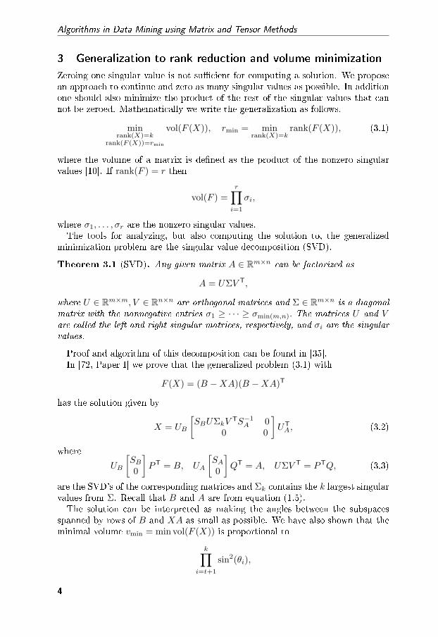
3 Generalization to rank reduction and volume minimization
Zeroing one singular value is not su�cient for computing a solution. We proposean approach to continue and zero as many singular values as possible. In additionone should also minimize the product of the rest of the singular values that cannot be zeroed. Mathematically we write the generalization as follows.
minrank(X)=k
rank(F (X))=rmin
vol(F (X)), rmin = minrank(X)=k
rank(F (X)), (3.1)
where the volume of a matrix is de�ned as the product of the nonzero singularvalues [10]. If rank(F ) = r then
vol(F ) =r∏i=1
σi,
where σ1, . . . , σr are the nonzero singular values.The tools for analyzing, but also computing the solution to, the generalized
minimization problem are the singular value decomposition (SVD).
Theorem 3.1 (SVD). Any given matrix A ∈ Rm×n can be factorized as
A = UΣV T,
where U ∈ Rm×m, V ∈ Rn×n are orthogonal matrices and Σ ∈ Rm×n is a diagonalmatrix with the nonnegative entries σ1 ≥ · · · ≥ σmin(m,n). The matrices U and Vare called the left and right singular matrices, respectively, and σi are the singularvalues.
Proof and algorithm of this decomposition can be found in [35].In [72, Paper I] we prove that the generalized problem (3.1) with
F (X) = (B −XA)(B −XA)T
has the solution given by
X = UB
[SBUΣkV TS−1
A 00 0
]UTA, (3.2)
where
UB
[SB0
]PT = B, UA
[SA0
]QT = A, UΣV T = PTQ, (3.3)
are the SVD's of the corresponding matrices and Σk contains the k largest singularvalues from Σ. Recall that B and A are from equation (1.5).The solution can be interpreted as making the angles between the subspaces
spanned by rows of B and XA as small as possible. We have also shown that theminimal volume vmin = min vol(F (X)) is proportional to
k∏i=t+1
sin2(θi),
4

ii
�phdBerkant� � 2008/4/28 � 10:32 � page 5 � #19 ii
ii
ii
Introduction and overview
where θi are the principal angles between the subspaces spanned by rows of P andQ. The integer parameter t indicates the size of the rank reduction in F (X). Ift = 0 then, of course, the volume reduces to the determinant.In the next section we apply this generalized criterion on problems from system
identi�cation.
4 Application to system identi�cation
The objective in system identi�cation is to determine mathematical models ofdynamical systems and processes based on measured observations. A system inthis context could be an aircraft, a power plant or a car engine. Systems havethe characteristics that they can be in�uenced by input signals1 and depending ontheir inherent state they produce measurable output data. The measured inputand output signals serve as source data in the computation of the model thatrelates the input signals to the output signals. The computed models are oftenused for control and simulations.There are many di�erent approaches to deal with system identi�cation problems.
A straight forward approach is to describe the present output at time t as a linearcombination of previous inputs and outputs,
y(t) = a1y(t− 1) + · · ·+ any(t− n) + b1u(t− 1) + · · ·+ bmu(t−m).
Here we assume that the signals are sampled and use n and m previous samplesof the output signal y and input signal u, respectively. A second approach is todescribe a system as a state-space model2,
x(t+ 1) = Ax(t) +Bu(t),y(t) = Cx(t) +Du(t),
where x is the state vector and the matrices A, B, C and D, which describe thesystem, are to be determined during the identi�cation process.In many cases, given an input sequence, there is a di�erence in the output
of the model compared to the actual output of the system. The constructedmodels attempt to minimize this di�erence in some measure. There are many otherapproaches and aspects concerning system identi�cation with extensive literaturebackground. A good overview is found in [59].The second paper in this thesis [75, Paper II] uses the generalized rank reduction
and volume minimization criterion in the framework of state-space subspace systemidenti�cation, which can be seen as a linear regression multi-step ahead predictionerror method [44]. The matrix form of the linear regression model can be written
Yα = L1Yβ + L2Uβ + L3Uα + Eα,
where Uα, Uβ are matrices with α future and β past input signals, Yα, Yβ are,similarly, future and past output signals, and L1, L2, L3 are the sought regression
1Input signals can often be speci�ed but they can also include disturbances and noise.2Actually this model contains additive noise terms in both equations but they are omitted
here.
5

ii
�phdBerkant� � 2008/4/28 � 10:32 � page 6 � #20 ii
ii
ii
Algorithms in Data Mining using Matrix and Tensor Methods
matrices. Computing the regression matrices gives the extended observabilitymatrix from which the state-space matrices can be extracted. The rank constrainton the regression matrices comes from the order of the system matrix A.Assuming that the input signal matrix Uα has full row rank3 we can eliminate
L3 from the equations, and write the regression problem in the same form as (1.5),where now [L1 L2] is the regression matrix.Without any assumptions on the measured signal matrices involved in the re-
gression we identify three di�erent scenarios where the determinant criterion isnot su�cient. These are:
1. Absence of noise in all or part of the output signals,2. Collinear output signals,3. Direct linear dependencies between input and output signals.
We have demonstrated the validity of our algorithm using numerical experimentsin a series of di�erent situations, including cases with rank de�cient and collineardata matrices. The generalized criterion gives the correct estimates in both thefull rank case and the rank de�cient case.In applications the rank of the regression matrix [L1 L2] (or X) is often unknown
and has to be determined. One additional advantage of our algorithm is that theappropriate rank can be chosen during the identi�cation process by analyzing thesingular values of PTQ, see equations (3.3) and (3.2).
5 Tensors and numerical multilinear algebra
5.1 Introduction to tensors
In numerical linear algebra, matrix computations and other mathematical scienceswe mostly use quantities as vectors x ∈ Rn and matrices A ∈ Rm×n for manydi�erent purposes. Vectors are usually elements of a vector space and matricesrepresent linear operators with respect to some basis, as the Hessian of a real valuedfunction. Matrices also represent measured data, as a digital image or a collectionof sensor signals. A vector is written as a one dimensional array of numbers andsingle index is used to address its entries. Similarly, a matrix is written as a twodimensional array of numbers whose entries are accessed with two indices.An order n tensor A ∈ RI1×···×In is a generalization of these algebraic objects
to one with n indices. Vectors and matrices are in fact �rst and second ordertensors, respectively. The dimension of A along the di�erent modes (or �directions�as rows and columns in a matrix) are given by Ii. Tensors are often found indi�erential geometry where they most of the time (if not exclusively) represent(abstract) multilinear operators. In this thesis tensors will, most of the time,constitute multidimensional data arrays, which we want to analyze, model andextract information from. In general tensors are di�cult to visualize but we canimagine order three tensors as in Figure 5.1. The modes in a tensor have di�erentmeanings in di�erent applications [73, 29, 86, 64, 21, 60]. Table 5.1 gives a fewexamples of their meanings. As we see these are essentially di�erent properties ofthe data and it is unnatural to reshape the tensor into a matrix.
3In a controlled experiments one can chose input signals to ful�ll this assumption.
6

ii
�phdBerkant� � 2008/4/28 � 10:32 � page 7 � #21 ii
ii
ii
Introduction and overview
1-mode
2-mode
3-mod
e
Figure 5.1: Visualization of an order three tensor.
It is important to distinguish the notation of tensors in the same way we dis-tinguish matrices (written with capital letters) and vectors (written in lower caseletters) in order to clarify the presentation. For this reason we will use capitalletters with calligraphic font (A,B, . . . ) to denote tensors.The usual way to analyze such data is to reshape the data into matrices and
vectors and use the well developed theory of numerical linear algebra. On the otherhand, we can �nd bene�ts in preserving the underlying structure of the data usingtheory and algorithms from numerical multilinear algebra. Tensor theory has beenused for modeling in psychometrics and chemometrics [83, 39, 54, 55] for a longtime now. Recently tensors have started to attract the attention from other �eldsof science as well [21, 23, 57, 25, 5, 52, 17, 19, 13, 69, 88, 85, 86, 60, 61, 71]. Themain research topics are to analyze the basic properties of tensors, generalize theexisting linear algebra theory to include tensors and construct e�cient algorithms.The connection to applications is often very close.
5.2 Basic operations, tensor properties and notation
In this section we give some of the basic operations and properties which are thebuilding blocks for the theory and algorithms. In the presentation we will usetensors of order three, four or �ve but the generalization to tensors of arbitraryorder is straightforward.Given a third order tensor A ∈ RI×J×K we write aijk to address its entries,
where the subscripts i, j, k are ranging from one to I, J,K, respectively. The
Application 1-mode 2-mode 3-modeHandwritten digit classi�cation pixels samples classesElectronic nose data sensors time gasesComputer vision persons pixel view/illuminationBioinformatics genes exp. variable microarray
Table 5.1: Examples of applications with tensors and the information content along thedi�erent modes.
7

ii
�phdBerkant� � 2008/4/28 � 10:32 � page 8 � #22 ii
ii
ii
Algorithms in Data Mining using Matrix and Tensor Methods
addition of two tensors A and B in RI×J×K is
C = A+ B, cijk = aijk + bijk.
The multiplication of a tensor A with a scalar γ is the tensor
B = γA, bijk = γaijk.
The inner product between two tensors A and B of same dimensions is the scalar
〈A,B〉 =∑i,j,k
aijkbijk.
The corresponding tensor norm is
‖A‖ = 〈A,A〉1/2 .We exclusively use this Frobenius norm in this thesis. The outer product betweentwo tensors A ∈ RI×J×K and B ∈ RL×M×N is an order six tensor,
RI×J×K×L×M×N 3 C = A ◦ B, cijklmn = aijkblmn.
This operation is a generalization of the outer product between vectors x and ywhich results in the matrix xyT.
5.3 Matrix-tensor multiplication
A matrix can be multiplied by other matrices on two sides � from left and fromright. An order n tensor can be multiplied with matrices along each one of itsmodes. For example, multiplication of an order three tensor A ∈ RI×J×K bymatrices X ∈ RL×I ,Y ∈ RM×J and Z ∈ RN×K is written and de�ned by
RL×M×N 3 B = (X,Y, Z) ·A, blmn =∑i,j,k
xliymjznkaijk.
If multiplication is done in just one or a few modes, we write
(X,Y )1,2 ·A = (X,Y, I) ·A.With this notation we can write standard matrix multiplication of three matrices as
XFY T = (X,Y ) · F.For convenience, we also introduce a separate notation for the multiplication by atransposed matrix U ∈ RI×L,
RL×J×K 3 C =(UT)
1·A = A · (U)1 , cljk =
∑i
aijkuil.
Multiplication in all modes with the transposed of the matrices U , V and W ofappropriate dimensions is analogous,(
UT, V T,WT) ·A = A · (U, V,W ) .
We want also to mention that there is a variety of notations for these manipula-tions, [47, 40, 23, 50, 17]. The notation we use for matrix-tensor products in allmodes was suggested in [25] and for matrix multiplication along a few modes weare inspired by [8].
8

ii
�phdBerkant� � 2008/4/28 � 10:32 � page 9 � #23 ii
ii
ii
Introduction and overview
5.4 Canonical tensor matricization
Another concept that is useful when working with tensors is the notion of matri-cizing, unfolding or �attening of a tensor. This is an operation for transforming agiven multidimensional array into a matrix. For example a 3-tensor A ∈ RI×J×Kcan be reshaped to form matrices of dimensions I × JK, J × IK or K × IJ andeach matrix has columns as speci�ed in Figure 5.2.
Figure 5.2: Matricizing a 3-tensor results in matrices where the columns of the respec-tive matrices are given by the illustrated �bers.
Di�erent matrices, with respect to column pivoting, will be obtained dependingon which order the tensor �bers in each case are taken into the matricized forms.Consider references [47, 23] for two di�erent examples. In [32, Paper IV] weintroduce a canonical way of matricizing a tensor which is directly related tothe matrix-tensor multiplication. For example, given a 5-tensor A and matricesV,W,X, Y, Z of appropriate dimensions, the matricization of the product B =A · (V,W,X, Y, Z) can be
B(2;1,3...5) ≡ B(2) = WTA(2)(V ⊗X ⊗ Y ⊗ Z), r = [2], c = [1, 3, 4, 5],
B(3,2;1,4,5) ≡ B(3,2) = (X ⊗W )TA(3,2)(V ⊗ Y ⊗ Z), r = [3, 2], c = [1, 4, 5],
where ⊗ denotes the Kronecker product and r and c indicate the modes of thetensors that are mapped to the rows and columns in the matrix form, respectively.This matricization has been very useful when analyzing, deriving expressions andimplementing algorithms for the Newton-Grassmann method. See [32, Section 2.2](page 92) for a detailed discussion and more examples.
5.5 Contracted products and multilinear algebraic manipulations
Matrix-vector, matrix-matrix, and also matrix-tensor products are all examplesof contracted products. It is necessary to generalize these products as well andde�ne contracted products between two general tensors. Contracted productsbetween tensors arise naturally when deriving the expressions for the gradientand the Hessian of an objective function for the low rank tensor approximationproblem, which we will consider in Section 6.2. The only requirement is that thedimensions of the contracting modes are equal. For example, givenA ∈ RI×J×K×L
9

ii
�phdBerkant� � 2008/4/28 � 10:32 � page 10 � #24 ii
ii
ii
Algorithms in Data Mining using Matrix and Tensor Methods
and B ∈ RI×L×M , we can de�ne
RJ×K×L×L×M 3 C = 〈A,B〉1 , cjkl1l2m =∑i
aijkl1bil2m, (5.1)
RJ×K×M 3 D = 〈A,B〉1,4;1,2 , djkm =∑i,l
aijklbilm. (5.2)
In our case the tensors involved in the contractions are actually matrix-tensorproducts, see equations (6.10), (6.11) and (6.12). In order to properly matricizethe derivative expressions for the algorithmic implementation of Newton and quasi-Newton methods, it is desirable to extract a matrix from a matrix-tensor product ina contraction. Given tensors B and C and a matrix Q with appropriate dimensionsthe following equality holds,
〈B · (Q)1 , C〉−2=⟨〈B, C〉−(1,2) , Q
⟩1,3;1,2
,
where negative contraction subscript indicates that all but the speci�ed modes arecontracted. This is a special case from [32, Lemma (2.3)].
6 Tensor rank and low rank tensor approximation
In many applications involving tensor data the objective is to compute low-rankapproximations of the data for modeling, information retrieval and explanatorypurposes, [24, 22, 25, 42, 78, 89, 18, 16, 46, 49, 48, 76, 81]. These approximationsare usually expressed in terms of tensor decompositions.By a rank-one tensor we mean a tensor that can be factorized as the outer
product of vectors. For example a 3-tensor of rank-one has the form A = x ◦ y ◦ z.Observe that with only two vectors x ◦ y = xyT we obtain a rank-one matrix. Therank of a tensor can be de�ned as the minimal number of terms when expressinga tensor as a sum of rank-one tensors.The second way to de�ne a rank of a tensor is given by the dimension of the
subspaces spanned by the di�erent n-mode vectors. Given an order n tensor A,we write
rank(A) = (r1, . . . , rn), ri = dim(
span(A(i)
)),
where A(i) is the matricization of A along mode i. This is called the multilinearrank of a tensor. For tensors in general the ranks ri are di�erent. For a matrix Awe have r1 = r2 = rank(A), since the row and column ranks of a matrix are equal.The theoretical properties of problems involving the multilinear rank of a tensorare much simpler than problems involving the outer-product tensor rank [25]. Itcan, for example, be shown that a sequence of rank-2 tensors can approximate arank-3 tensor arbitrary well. In this thesis we have only considered the problemof approximating a given tensor by another tensor of lower multilinear rank.The approximation problem of an order three tensor A ∈ RI×J×K is stated,
minB‖A − B‖, rank(B) = (r1, r2, r3). (6.1)
10

ii
�phdBerkant� � 2008/4/28 � 10:32 � page 11 � #25 ii
ii
ii
Introduction and overview
AC
XY T
ZT
≈
Figure 6.1: The approximation of a tensor A by another tensor B = (X, Y, Z) · C oflower multilinear rank.
Assuming the rank constraint on B, we can decompose B = (X,Y, Z) · C whereX ∈ RI×r1 , Y ∈ RJ×r2 , Z ∈ RK×r3 have full column rank and C ∈ Rr1×r2×r3 .This is a Tucker decomposition of a tensor [82, 83]. The approximation problem,as well as the decomposition of B are visualized in Figure 6.1. The decompositionof B is in fact a consequence of the higher order singular value decomposition(HOSVD) [23].
Theorem 6.1 (HOSVD). Any 3-tensor A ∈ RI×J×k can be factorized
A = (U, V,W ) · S, (6.2)
where U ∈ RI×I , V ∈ RJ×J , and W ∈ RK×K , are orthogonal matrices, andthe tensor S ∈ RI×J×K is all-orthogonal: the matrices 〈S,S〉−i, i = 1, 2, 3, arediagonal, and
‖S(1, :, :)‖ ≥ ‖S(2, :, :)‖ ≥ · · · ≥ 0, (6.3)
‖S(:, 1, :)‖ ≥ ‖S(:, 2, :)‖ ≥ · · · ≥ 0, (6.4)
‖S(:, :, 1)‖ ≥ ‖S(:, :, 2)‖ ≥ · · · ≥ 0, (6.5)
are the 1-mode, 2-mode, and 3-mode singular values, also denoted σ(1)i , σ
(2)i , σ
(3)i .
The tensor S in the HOSVD is in general full and not sparse or diagonal as Σin the SVD of a matrix, see Theorem 3.1. But the all-orthogonality concept isstill valid in matrix SVD. The singular values in (6.3) correspond to norms of rowvectors from Σ and those in (6.4) correspond to norms of column vectors, whichfor matrix SVD are equal since Σ is diagonal. In addition any two di�erent columnor row vectors from Σ are orthogonal to each other. The HOSVD is an importantresult both for analysis and applications with tensors since it gives an orderingof the basis vectors in U , V and W . The ordering also implies that elements oflargest magnitude in S are concentrated towards the (1, 1, 1) corner. The entriesin S generally decay when going away in all directions from this corner.In fact truncating the HOSVD, i.e. taking the �rst r1, r2 and r3 columns from
U , V and W , respectively and correspondingly truncating S, will give (hopefully)a good approximation of A. The di�erence compared to the matrix case is thatthe truncated HOSVD is not the solution of (6.1) [24]. From an application pointof view this may still be good enough for di�erent purposes.There are other higher order generalizations of the SVD, singular values/vectors
as well as eigenvalues/vectors of tensors [15, 39, 57, 66, 67, 68].
11

ii
�phdBerkant� � 2008/4/28 � 10:32 � page 12 � #26 ii
ii
ii
Algorithms in Data Mining using Matrix and Tensor Methods
6.1 Application of truncated higher order SVD to handwritten digit
classi�cation
Pattern recognition and classi�cation is one of the main topics in data mining andthere are many di�erent ways to approach and solve the encountered problems.Classical approaches are the nearest and k-nearest neighbor methods. The idea isto interpret objects as vectors or elements in a �nite dimensional linear space andcompute some kind of proximity measure between known and unknown objects.The label of the closest or k closest known objects determine the label of the un-known object to be classi�ed. A second and intuitive approach is to �nd linear ornonlinear functions partitioning the space into disjoint regions where objects fromdi�erent classes belong to a certain region. Other ways of solving pattern recogni-tion problems include linear algebra methods (least squares, eigenvalue problems,data compression and feature extraction by low rank approximation), statisticalmethods (maximum likelihood estimation, linear and nonlinear regression, sup-port vector machines) and neural networks. Good references for the mentionedmethods are [26, 41, 30].In [73, Paper III] we use the HOSVD for reduction of data consisting of hand-
written digits. The data have pixels along the �rst mode, samples along the secondmode and classes along the third mode. We show that we can make a 98% com-pression of the data without losing classi�cation performance. This is done byreducing the pixel dimension from 400 to 30�60 and the sample dimension from1000 to 30�60 as well. After the reduction each digit is described with only 30�60 pixels and only 30�60 samples represent the variation within each class. Theclass-models are given by the dominant pixel-subspaces obtained by regular SVDon the reduced data. An unknown digit is projected on each one of the 10 sub-spaces and the subspace with smallest residual gives the output of the algorithm.Straightforward implementation of this method gives a classi�cation error of 5%.
6.2 Best low rank tensor approximation
In [32, Paper IV] and [74, Paper V] we develop Newton and quasi-Newtonalgorithms for computing the best multilinear low-rank tensor approximation.Rewriting the tensor approximation problem (6.1) with the decomposition B =(X,Y, Z) · C we get
minX,Y,Z,C
‖A − (X,Y, Z) · C‖.
One can show that this problem is overparameterized and with little algebraicmanipulations we show (see [32, Section 3] and [24]) that the tensor approximationproblem is equivalent to
maxX,Y,Z
‖A · (X,Y, Z) ‖, (6.6)
where now the matrices X, Y and Z have orthonormal columns, i.e. XTX = Ir1 ,Y TY = Ir2 and ZTZ = Ir3 . In addition, expression (6.6) only depends on thesubspaces spanned by columns of X, Y and Z, thus it is invariant to the speci�cbasis representation of a subspace. In other words the following equality holds,
‖A · (X,Y, Z) ‖ = ‖A · (XU, Y V, ZW ) ‖,
12

ii
�phdBerkant� � 2008/4/28 � 10:32 � page 13 � #27 ii
ii
ii
Introduction and overview
where U , V andW are orthogonal matrices. It follows that the maximization prob-lem is de�ned on a product of three Grassmann manifolds. A point on a Grass-mann manifold Gr(n, r) consists of all n × r matrices with orthonormal columnsthat span the same subspace, we write
Gr(n, r) 3 [X] = {XU : U orthogonal}.
These observations lead to the following nonlinear maximization problem con-strained in the variables X, Y and Z;
max(X,Y,Z)∈Gr3
Φ(X,Y, Z), Gr3 = Gr(I, r1)×Gr(J, r2)×Gr(K, r3), (6.7)
where
Φ(X,Y, Z) =12‖A · (X,Y, Z)‖2 =
12
∑j,k,l
( ∑λ,µ,ν
aλµνxλjyµkzνl
)2
. (6.8)
This expression is a polynomial of degree six. In the next sections we will brie�ydescribe algorithms for maximizing Φ.
6.3 Optimization on a product of Grassmann manifolds
If the objective function in an optimization problem is de�ned on a manifold, oneneeds to take into account the nature of the manifold when constructing algorithms[27, 34, 3, 12, 77, 2, 1, 43]. In particular we need to modify:
1. The gradient and Hessian of the function,2. The update of the current iterate in a given direction,3. The update of a vector, if it is computed at one point on the manifold but
used on another point.These modi�cations are required both for theoretical and practical reasons. Allcomputations involved in the algorithms are performed on the tangent spaces fordi�erent points of the manifolds. Thus given a point X ∈ Gr(n, r) the gradient ofa function f(X) is a vector in the tangent space TX to the manifold at X, i.e.
∇f(X) ∈ TX .
Similarly, the Grassmann Hessian Hf of the function f at X is an operator map-ping vectors from TX to vectors in TX ,
Hf : TX → TX .
If we consider the objective function for the tensor approximation problem,Φ(X,Y, Z), we will have three di�erent tangent spaces, TX , TY and TZ . In thiscase the Hessian will involve linear operators from each tangent space to everyother tangent space. Writing the Hessian of Φ as
HΦ =
Hxx Hxy Hxz
Hyx Hyy Hyz
Hzx Hzy Hzz
,
13

ii
�phdBerkant� � 2008/4/28 � 10:32 � page 14 � #28 ii
ii
ii
Algorithms in Data Mining using Matrix and Tensor Methods
we will have Hxx : TX → TX , Hxy : TY → TX , Hzy : TY → TZ and similarlyfor the other parts. On manifolds we choose to move from a point along geodesiccurves that are de�ned by the direction of movement, which is vector in the tangentspace. The geodesic never leaves the manifold and corresponds to a straight line inEuclidean spaces. Given a point X ∈ Gr(n, r) and direction ∆ ∈ TX , the explicitexpression of a geodesic on the Grassmann manifold has the form
X∆(t) = XV cos(tΣ)V T + U sin(tΣ)V T, (6.9)
where U , Σ and V are obtained from the thin singular value decomposition of ∆.If there is a second tangent vector ∆2 at X the parallel transport of it along thegeodesic is given by
TX(t) 3 ∆2(t) =((XV U
)(− sin Σtcos Σt
)UT + (I − UUT)
)∆2.
This kind of parallel transport is necessary in quasi-Newton algorithms. For ex-ample in Euclidean space we would need to compute ∇f(X1) − ∇f(X2) but onmanifolds the two terms are de�ned on di�erent points of the manifold, and thusbelong to di�erent tangent spaces. In order to perform this computation we haveto parallel transport one of the gradients to the tangent space of the other, thenwe can perform the subtraction.
6.4 The Grassmann gradient and the the Grassmann Hessian
The expressions for the gradient and the Hessian of a function are derivedfrom the Taylor expansion, in which the linear term gives the gradient and thequadratic term gives the Hessian. With the following terms F = A · (X,Y, Z),Bx = A · (X⊥, Y, Z), By = A · (X,Y⊥, Z) and Bz = A · (X,Y, Z⊥) we can writethe Grassmann gradient in local coordinates as
∇Φ =(⟨Bx,F
⟩−1,⟨By,F
⟩−2,⟨Bz,F
⟩−3
). (6.10)
The matrices X⊥, Y⊥ and Z⊥ are the orthogonal complements of X, Y and Z,respectively. The columns of the orthogonal complements form in fact a basis foreach tangent space, for example TX = span(X⊥). One can also show that thefollowing eigenspace-like equations are valid at a stationary point of the objectivefunction, i.e. when ∇Φ = 0,
〈A · (I, Y, Z) ,A · (I, Y, Z)〉−1X = X 〈F ,F〉−1 ,
〈A · (X, I, Z) ,A · (X, I, Z)〉−2Y = Y 〈F ,F〉−2 ,
〈A · (X,Y, I) ,A · (X,Y, I)〉−3 Z = Z 〈F ,F〉−3 .
Writing the gradient in matrix form yields,⟨Bx,F
⟩−1
= XT⊥A
(1)(Y ⊗ Z)(Y ⊗ Z)T(A(1))TX,⟨By,F
⟩−2
= Y T⊥A
(2)(X ⊗ Z)(X ⊗ Z)T(A(2))TY,⟨Bz,F
⟩−2
= ZT⊥A
(3)(X ⊗ Y )(X ⊗ Y )T(A(3))TZ,
14

ii
�phdBerkant� � 2008/4/28 � 10:32 � page 15 � #29 ii
ii
ii
Introduction and overview
where A(1), A(2) and A(3) are matricizations of A.The Grassmann Hessian is more complex than the gradient, but it also has
a symmetric structure and consists of contracted tensor products. Here we givetwo blocks of the Hessian operator acting on tangent vectors4 Dx, Dy and visualizehow they are computed. In local coordinate the xx- and xy-part of the GrassmannHessian acting on coordinate matrices have the form
Hxx(Dx) =⟨Bx, Bx
⟩−1Dx −Dx 〈F ,F〉−1 , (6.11)
Hxy(Dy) =⟨⟨Cxy,F
⟩−(1,2)
, Dy
⟩2,4;1,2
+⟨⟨Bx, By
⟩−(1,2)
, Dy
⟩4,2;1,2
, (6.12)
where we also introduce Cxy = A · (X⊥, Y⊥, Z). Figure 6.2 shows all tensor-matrix products involved in the computation of the Hessian. These are blocks of
A · (X, Y, Z)
A · (X⊥, Y, Z)
A · (X, Y⊥, Z)
A · (X⊥, Y⊥, Z)
A · (X, Y, Z⊥)
A · (X⊥, Y, Z⊥)
A · (X, Y⊥, Z⊥)
A · (X⊥, Y⊥, Z⊥)
Figure 6.2: Illustration of the tensor-matrix products involved in the computation ofthe Hessian. The matrix slices are used to compute xx-part and the �bers along thethird mode are used to compute xy-part of the Hessian.
A · ((XX⊥), (Y Y⊥), (Z Z⊥)). Recall that the objective is to maximize the normof A · (X,Y, Z).The �rst term in (6.11) is a matrix since it is a contraction in all but the �rst
mode between Bx and itself. Each entry in the resulting matrix is the scalarproduct between two slices in A · (X⊥, Y, Z). Similarly, the second term 〈F ,F〉−1
is also a matrix whose elements are di�erent scalar products between slices ofA · (X,Y, Z). See the corresponding blocks in Figure 6.2.The �rst term in (6.12) involves two di�erent contractions resulting in a matrix.
The �rst one is a contraction between the 3-tensors Cxy and F in all but the �rstand second mode, thus in this case contraction in the third mode. This resultsin a 4-tensor whose elements are scalar products between third mode �bers fromeach tensor. In Figure 6.2 these are illustrated with the symbol. In the
4These are actually matrices but represent the coordinates of elements on the tangent space.
15

ii
�phdBerkant� � 2008/4/28 � 10:32 � page 16 � #30 ii
ii
ii
Algorithms in Data Mining using Matrix and Tensor Methods
Figure 6.3: Illustration of the sparsity pattern in the matricized Hessian. The diagonalblocks are sparse but these are coupled tightly together with non-sparse o�-diagonalblocks.
second contraction we multiply the 4-tensor 〈Cxy,F〉−(1,2) with the matrix Dy andcontract second and fourth mode of the tensor with the �rst and second mode ofthe matrix which results in a matrix. Similarly, in the second term of (6.12), thethird mode contractions are done between the tensors Bx = A · (X⊥, Y, Z) andBy = A · (X,Y⊥, Z), these are symbolized with in Figure 6.2.The remaining blocks of the Hessian are computed in a analogous fashion. The
contractions are in other modes and involve other matrix-tensor product blocks.Consider Sections 4.2 and 4.3 in [32] for further details.The zero structure of the matricized Hessian is given in Figure 6.3 for a test
example of a 10×9×12 tensor approximated by a rank-(3, 4, 5) tensor. Introducingzeros in the matrices X,Y, Z and the basis X⊥, Y⊥, Z⊥ for the tangent spacesTX ,TY ,TZ , respectively, by applying coordinate transformations does not resultin a sparser Hessian structure.
6.5 Newton-Grassmann and quasi-Newton-Grassmann algorithms
In this thesis we introduce three new methods for computing the best low rankapproximation of a tensor; a Newton-Grassmann algorithm, a quasi-Newton-Grassmann algorithm based on the BFGS updates and an algorithm based on thelimited memory BFGS updates. These are standard algorithms for unconstrainedoptimization problems [63]. The novelty in this presentation is the incorporation ofthe product Grassmann manifold structure, inherent in the tensor approximationproblem, into the algorithms.
16

ii
�phdBerkant� � 2008/4/28 � 10:32 � page 17 � #31 ii
ii
ii
Introduction and overview
The iterative framework of the three algorithms is similar and originates fromthe Newton equations,
Hkpk = −∇fk, (6.13)
which is derived from a second order Taylor approximation of an objective func-tion f(x) with goal to maximize it. The algorithms are started with an initialapproximation x0 of a local minimizer and in each iteration one computes a di-rection of movement pk. A better approximation is obtained with the updatexk+1 = xk + tkpk, where tk is step length of movement. Of course, if xk is apoint on a manifold then the appropriate update is to move along a geodesic inthe direction pk. Figure 6.4 illustrates this on the Grassmann manifold Gr(3, 1)which is simply the sphere in R3. The computations of the direction of movements
Figure 6.4: Illustration of geodesic movement form X1 in the direction given by ∆1.This is part of a sphere in R3 which is the Grassmann manifold Gr(3, 1). The geodesicson the sphere are given by great circles. Also the squares indicate the tangent spaces atwhich the computations are performed.
are performed on the tangent spaces, illustrated with a square, at each iterate andthe update is a movement along the great circles de�ned by the tangent vectors,∆1 and ∆2 in Figure 6.4.The di�erent algorithms di�er in the way Hk is computed. In Newton's method
Hk is the exact Hessian computed at each new iterate. In quasi-Newton meth-ods one instead updates the current Hessian approximation by a rank-2 matrixmodi�cation. One looses on convergence rate but gains in computation time.Quasi-Newton methods with BFGS updates are recognized to be one of the bestperforming algorithms for general medium sized unconstrained nonlinear optimiza-tion problems [63]. If the problems are large the actual Hessian approximationHk ∈ Rn×n may be too big to �t in the computer memory. In limited memoryBFGS methods this is overcome by expressing Hk in a compact form using veryfew vectors of size n, [14].Figure 6.5 contains two plots illustrating the convergence of the di�erent algo-
rithms compared to higher order orthogonal iteration (HOOI), which is related toalternating least square methods (ALS). The setup for the left �gure is as follows:
17

ii
�phdBerkant� � 2008/4/28 � 10:32 � page 18 � #32 ii
ii
ii
Algorithms in Data Mining using Matrix and Tensor Methods
0 20 40 60 80 10010
−15
10−10
10−5
RE
LAT
IVE
NO
RM
OF
TH
E G
RA
DIE
NT
ITERATION #
BFGSL−BFGSHOOING
200 300 400 500 600 700 80010
−15
10−10
10−5
RE
LAT
IVE
NO
RM
OF
TH
E G
RA
DIE
NT
ITERATION #
BFGSL−BFGSHOOI
Figure 6.5: Left: A 20× 20× 20 tensor with random entries (N(0, 1)) is approximatedwith a rank-(5, 5, 5) tensor. Right: A 100×100×100 tensor with random entries (N(0, 1))is approximated with a rank-(5, 10, 20) tensor.
A random tensor A ∈ R20×20×20 with random entries (N(0, 1)) is approximatedwith a rank-(5, 5, 5) tensor. All algorithms are initialized with truncated HOSVD.The QNmethod with BFGS updates was initialized with the exact Hessian whereasthe limited memory BFGS algorithm uses scaled identity matrix as initial Hessianapproximation. We observe a quadratic convergence for the Newton-Grassmannalgorithm and superlinear convergence for the BFGS algorithm. The right �gureshows convergence for a random tensor A ∈ R100×100×100 approximated with arank-(5, 10, 20) tensor. All three algorithms are initiated with truncated HOSVDand 50 HOOI iterations. Both BFGS and L-BFGS methods used a scaled identityas initial Hessian approximation. The second problem is too big for the Newton-Grassmann algorithm, therefore not present in the right �gure.
7 Future research directions
In this section I will give a short presentation with open questions on di�erentresearch topics related to tensors.
7.1 Multilinear systems of equations
The theoretical properties of systems of multilinear equations need to be investi-gated. Consider the generalization
A · (y, z)2,3 = b ⇔ A(1) (y ⊗ z) = b,
where A ∈ RI×J×K and b ∈ RI are given while y ∈ RJ and z ∈ RK are unknown.What properties of A and b determine the existence of a solution? Obviously it isnot enough for b to belong to the range space of A(1). If the multilinear equationsare consistent when is the solution unique? Is there a close form solution? Whatabout solutions to
miny,z‖A · (y, z)2,3 − b‖ ⇔ min
y,z‖A(1) (y ⊗ z)− b‖.
Generalizing these equations to involve higher order tensors is obvious.
18
ii
�phdBerkant� � 2008/4/28 � 10:32 � page 19 � #33 ii
ii
ii
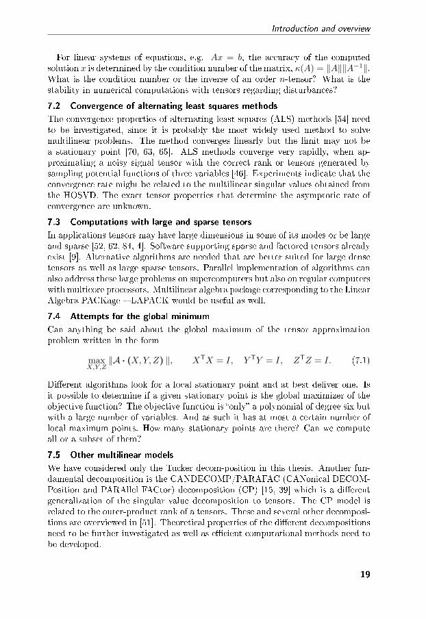
Introduction and overview
For linear systems of equations, e.g. Ax = b, the accuracy of the computedsolution x is determined by the condition number of the matrix, κ(A) = ‖A‖‖A−1‖.What is the condition number or the inverse of an order n-tensor? What is thestability in numerical computations with tensors regarding disturbances?
7.2 Convergence of alternating least squares methods
The convergence properties of alternating least squares (ALS) methods [54] needto be investigated, since it is probably the most widely used method to solvemultilinear problems. The method converges linearly but the limit may not bea stationary point [70, 63, 65]. ALS methods converge very rapidly, when ap-proximating a noisy signal tensor with the correct rank or tensors generated bysampling potential functions of three variables [46]. Experiments indicate that theconvergence rate might be related to the multilinear singular values obtained fromthe HOSVD. The exact tensor properties that determine the asymptotic rate ofconvergence are unknown.
7.3 Computations with large and sparse tensors
In applications tensors may have large dimensions in some of its modes or be largeand sparse [52, 62, 84, 4]. Software supporting sparse and factored tensors alreadyexist [9]. Alternative algorithms are needed that are better suited for large densetensors as well as large sparse tensors. Parallel implementation of algorithms canalso address these large problems on supercomputers but also on regular computerswith multicore processors. Multilinear algebra package corresponding to the LinearAlgebra PACKage � LAPACK would be useful as well.
7.4 Attempts for the global minimum
Can anything be said about the global maximum of the tensor approximationproblem written in the form
maxX,Y,Z
‖A · (X,Y, Z) ‖, XTX = I, Y TY = I, ZTZ = I. (7.1)
Di�erent algorithms look for a local stationary point and at best deliver one. Isit possible to determine if a given stationary point is the global maximizer of theobjective function? The objective function is �only� a polynomial of degree six butwith a large number of variables. And as such it has at most a certain number oflocal maximum points. How many stationary points are there? Can we computeall or a subset of them?
7.5 Other multilinear models
We have considered only the Tucker decom-position in this thesis. Another fun-damental decomposition is the CANDECOMP/PARAFAC (CANonical DECOM-Position and PARAllel FACtor) decomposition (CP) [15, 39] which is a di�erentgeneralization of the singular value decomposition to tensors. The CP model isrelated to the outer-product rank of a tensors. These and several other decomposi-tions are overviewed in [51]. Theoretical properties of the di�erent decompositionsneed to be further investigated as well as e�cient computational methods need tobe developed.
19

ii
�phdBerkant� � 2008/4/28 � 10:32 � page 20 � #34 ii
ii
ii
ii
�phdBerkant� � 2008/4/28 � 10:32 � page 21 � #35 ii
ii
ii
2Summary of papers
Paper I
Dimensionality reduction and volume minimization � generalization of the
determinant minimization criterion for reduced rank regression problems
In this paper we generalize the determinant minimization criterion for thereduced rank regression problem into dimensionality reduction of the objectivematrix and then volume minimization, where volume of a matrix is de�ned as theproduct of its nonzero singular values [10]. The determinant criterion is appealingsince it is closely related to maximum likelihood estimation [59, 44] but it hasimplicit assumptions not allowing rank de�ciency in the objective matrix [80, 87].The analysis reveals several cases where rank de�ciency is obtained.
Paper II
Rank reduction and volume minimization approach to state-space subspace
system identi�cation
In the second paper we consider the generalized minimization criterion for thereduced rank regression problem in the context of state-space subspace systemidenti�cation. The theoretical background of the algorithms solving the regressionproblem rely on the presence of noise to ensure that the full rank assumption isful�lled [80, 44]. If this is not true both the theory and algorithm will fail andyet there are cases where rank de�ciency is only natural. We identify the di�erentcases of rank de�ciency in terms of properties in the measured signals. We alsoshow that the given algorithm deals implicitly with all these cases.
Paper III
Handwritten digit classi�cation using higher order singular value
decomposition
In this paper we discuss two classi�cation algorithms based on higher ordersingular value decomposition (HOSVD) [23]. The �rst algorithm uses HOSVDto construct a set of orthonormal basis matrices spanning the dominant subspacefor each class. The basis matrices serve as models for the di�erent classes. Clas-si�cation is conducted by expressing the unknown digit as a linear combination
21

ii
�phdBerkant� � 2008/4/28 � 10:32 � page 22 � #36 ii
ii
ii
Algorithms in Data Mining using Matrix and Tensor Methods
with class speci�c basis matrices. In the second algorithm HOSVD is used tomake a data reduction prior the construction of the class models. The achievedclassi�cation rate is 95% despite the 98%�99% data reduction.
Paper IV
A Newton-Grassmann method for computing the best multilinear
rank-(r1, r2, r3) approximation of a tensor
In this paper we derive a Newton method for computing the best rank-(r1, r2, r3) approximation of a given I × J ×K tensor A. The problem is formu-lated as an optimization problem de�ned on a product of Grassmann manifolds.Incorporating the manifold structure into Newton's method ensures that all it-erates generated by the algorithm are points on the Grassmann manifolds. Wealso introduce a consistent notation for matricizing a tensor, for contracted tensorproducts and some tensor-algebraic manipulations, which simplify the derivationof the Newton equations and enable straightforward algorithmic implementation.Experiments show a quadratic convergence rate for the Newton-Grassmann algo-rithm.
Paper V
Best multilinear rank approximation of tensors with quasi-Newton methods
on Grassmannians
In this report we present quasi-Newton methods for computing the best rank-(r1, r2, r3) approximation of a given tensor. Both the general and the symmetriccase are considered. We consider algorithms based on BFGS and limited memoryBFGS updates modi�ed to operate on a product of Grassmann manifolds. We givea complexity analysis of the di�erent algorithms both in local and global coordi-nate implementations. The presented BFGS algorithms are compared with theNewton-Grassmann and alternating least squares (ALS) methods. Experimentsshow that the performance of the quasi-Newton methods is much better than theother methods when applied on di�cult problems.
22

ii
�phdBerkant� � 2008/4/28 � 10:32 � page 23 � #37 ii
ii
ii
References
[1] P.-A. Absil, C. G. Baker, and K. A. Gallivan. Trust-region methods on Rie-mannian manifolds. Foundations of Computational Mathematics, 7(3):303�330, 2007.
[2] P.-A. Absil, R. Mahony, and R. Sepulchre. Riemannian geometry of Grass-mann manifolds with a view on algorithmic computation. Acta Appl. Math.,80(2):199�220, 2004.
[3] P.-A. Absil, R. Mahony, and R. Sepulchre. Optimization Algorithms on MatrixManifolds. Princeton University Press, Princeton, NJ, January 2008.
[4] E. Acar and B. Yener. Unsupervised multiway data analysis: A literature sur-vey. Technical report, Computer Science Department, Rensselaer PolytechnicInstitute, 2007.
[5] O. Alter, P.O. Brown, and D. Botstein. Generalized singular value decom-position for comparative analysis of genome-scale expression data sets of twodi�erent organisms. PNAS, 100(6):3351�3356, March 2003.
[6] T. W. Anderson. Canonical correlation analysis and reduced rank regressionin autoregressive models. Ann. Statist., 30(4):1134�1154, 2002.
[7] T. W. Anderson. An Introduction to Multivariate Statistical Analysis. WileyInterscience, 3 edition, 2003.
[8] B. W. Bader and T. G. Kolda. Algorithm 862: MATLAB tensor classes forfast algorithm prototyping. ACM Trans. Math. Softw., 32(4):635�653, 2006.
[9] B. W. Bader and T. G. Kolda. E�cient MATLAB computations with sparseand factored tensors. SIAM Journal on Scienti�c Computing, 30(1):205�231,2007.
[10] A. Ben-Israel. A volume associated with m×n matrices. Linear Algebra andits Applications, 167:87�111, 1992. Sixth Haifa Conference on Matrix Theory(Haifa, 1990).
[11] Å. Björck. Numerical Methods for Least Squares Problems. Society for Indus-trial and Applied Mathematics (SIAM), Philadelphia, PA, 1996.
23

ii
�phdBerkant� � 2008/4/28 � 10:32 � page 24 � #38 ii
ii
ii
Algorithms in Data Mining using Matrix and Tensor Methods
[12] W. M. Boothby. An Introduction to Di�erentiable Manifolds and RiemannianGeometry, volume 120 of Pure and Applied Mathematics. Academic Press Inc.,Orlando, FL, second edition, 1986.
[13] R. Bro. Multi-way Analysis in the Food Industry Models, Algorithms, andApplications. PhD thesis, University of Amsterdam (NL), 1998.
[14] R. H. Byrd, J. Nocedal, and R. B. Schnabel. Representations of quasi-Newtonmatrices and their use in limited memory methods. Math. Programming, 63(2,Ser. A):129�156, 1994.
[15] J. D. Carroll and J. J. Chang. Analysis of individual di�erences in multidimen-sional scaling via an n-way generalization of �Eckart-Young� decomposition.Psychometrika, 35:Psychometrika, 1970.
[16] S. R. Chinnamsetty, M. Espig, B. N. Khoromskij, and W. Hackbusch. Tensorproduct approximation with optimal rank in quantum chemistry. The Journalof Chemical Physics, 127(084110):14, 2007.
[17] P. Comon. Tensor decompositions. In J. G. McWhirter and I. K. Proudler,editors, Mathematics in Signal Processing V, pages 1�24. Clarendon Press,Oxford, UK, 2002.
[18] P. Comon, G. Golub, L.-H. Lim, and B. Mourrain. Symmetric tensor andsymmetric tensor rank. SIAM J. Matrix Anal. Appl. to appear.
[19] P. Comon, G. Golub, L.-H. Lim, and B. Mourrain. Genericity and rankde�ciency of high order symmetric tensors. In Proceedings of the IEEE In-ternational Conference on Acoustics, Speech, and Signal Processing (ICASSP'06), volume 31, pages 125�128, 2006.
[20] D. J. Cook and L. B. Holder, editors. Mining Graph Data. Wiley, 2007.
[21] L. De Lathauwer. Signal Processing Based on Multilinear Algebra. PhD thesis,K. U. Leuven, Department of Electrical Engineering (ESAT), 1997.
[22] L. De Lathauwer, L. Hoegaerts, and J. Vandewalle. A Grassmann-Rayleighquotient iteration for dimensionality reduction in ICA. In Proc. 5th Int.Workshop on Independent Component Analysis and Blind Signal Separation(ICA 2004), pages 335�342, Granada, Spain, Sept. 2004.
[23] L. De Lathauwer, B. De Moor, and J. Vandewalle. A multilinear singularvalue decomposition. SIAM Journal on Matrix Analysis and Applications,21(4):1253�1278, 2000.
[24] L. De Lathauwer, B. De Moor, and J. Vandewalle. On the best rank-1 andrank-(R1, R2, . . . , RN ) approximation of higher-order tensors. SIAM Journalon Matrix Analysis and Applications, 21(4):1324�1342, 2000.
[25] V. de Silva and L.-H. Lim. Tensor rank and the ill-posedness of the bestlow-rank approximation problem. SIAM J. Matrix Anal. Appl., to appear,2007.
24

ii
�phdBerkant� � 2008/4/28 � 10:32 � page 25 � #39 ii
ii
ii
References
[26] R. O. Duda, P. E. Hart, and D. G. Stork. Pattern Classi�cation. Wiley-Interscience, New York, second edition, 2001.
[27] A. Edelman, T.A. Arias, and S.T. Steven. The geometry of algorithms withorthogonality constraints. SIAM J. Matrix Anal. Appl., 20(2):303�353, 1999.
[28] L. Eldén. Numerical linear algebra in data mining. Acta Numerica, 15:327�384, 2006.
[29] L. Eldén. Decomposition of a 3-way array of data from the electronic nosebaseline�corrected data. Manuscript, March 2002.
[30] L. Eldén. Matrix Methods in Data Mining and Pattern Recognition. SIAM,2007.
[31] L. Eldén and B. Savas. The maximum likelihood estimate in reduced-rankregression. Numerical Linear Algebra with Applications, 12:731�741, 2005.
[32] L. Eldén and B. Savas. A Newton-Grassmann method for computing thebest multilinear rank-(r1, r2, r3) approximation of a tensor. Technical ReportLITH-MAT-R-2007-6-SE, Department of Mathematics, Linköpings Univer-sitet, 2007.
[33] I. Foster. The grid: A new infrastructure for 21st century science. PhysicsToday, 2002.
[34] D. Gabay. Minimizing a di�erentiable function over a di�erential manifold.Journal of Optimization Theory and Applications, 37(2):177�219, 1982.
[35] G. H. Golub and C. F. Van Loan. Matrix Computations. Johns Hopkins Stud-ies in the Mathematical Sciences. Johns Hopkins University Press, Baltimore,MD, third edition, 1996.
[36] R. L. Grossman, C. Kamath, P. Kegelmeyer, V. Kumar, and R. R. Naburu,editors. Data Mining for Scienti�c and Engineering Applications, Massivecomputing. Kluwer Academic Publishers, 2001.
[37] J. Han and M. Kamber. Data Mining: Concepts and Techniques. MorganKaufmann Publishers, San Francisco, 2001.
[38] D. Hand, H. Mannila, and P. Smyth. Principles of Data Mining. MIT Press,Cambridge, MA, 2001.
[39] R. A. Harshman. Foundations of the PARAFAC procedure: Models andconditions for an "explanatory" multi-modal factor analysis. UCLA WorkingPapers in Phonetics, 16:1�84, 1970.
[40] R. A. Harshman. An index formalism that generalizes the capabilities ofmatrix notation and algebra to n-way arrays. J. Chemometrics, (15):689�714, 2001.
25

ii
�phdBerkant� � 2008/4/28 � 10:32 � page 26 � #40 ii
ii
ii
Algorithms in Data Mining using Matrix and Tensor Methods
[41] T. Hastie, R. Tibshirani, and J Friedman. The Elements of Statistical Learn-ing. Springer Series in Statistics. Springer-Verlag, New York, 2001.
[42] F. L. Hitchcock. Multiple invariants and generalized rank of a p-way matrixor tensor. J. Math. Phys. Camb., 7:39�70, 1927.
[43] M. Ishteva, L. De Lathauwer, P.-A. Absil, and S. Van Hu�el. Dimensionalityreduction for higher-order tensors: algorithms and applications. Internal Re-port 07-187, ESAT-SISTA, K.U.Leuven (Leuven, Belgium), 2007. submittedto: International Journal of Pure and Applied Mathematics.
[44] M. Jansson and B. Wahlberg. A linear regression approach to state-spacesubspace system identi�cation. Signal Processing, 52:103�129, 1996.
[45] C. Kamath. On mining scienti�c datasets. In R. L. Grossman, C. Kamath,P. Kegelmeyer, V. Kumar, and Namburu R. R., editors, Data Mining ForScienti�c and Engineering Applications. Kluwer Academic Publishers, 2001.
[46] B. N. Khoromskij and V. Khoromskaia. Low rank Tucker-type tensor approx-imation to classical potentials. Central European Journal of Mathematics,5(3):523�550, 2007.
[47] H. A. L. Kiers. Towards a standardized notation and terminology in multiwayanalysis. Journal of Chemometrics, 14:106�125, 2000.
[48] T. G. Kolda. Orthogonal tensor decompositions. SIAM Journal on MatrixAnalysis and Applications, 23(1):243�255, 2001.
[49] T. G. Kolda. A counterexample to the possibility of an extension of the Eckart-Young low-rank approximation theorem for the orthogonal rank tensor de-composition. SIAM Journal on Matrix Analysis and Applications, 24(3):762�767, 2003.
[50] T. G. Kolda. Multilinear operators for higher-order decompositions. TechnicalReport SAND2006-2081, Sandia National Laboratories, April 2006.
[51] T. G. Kolda and B. W. Bader. Tensor decompositions and applications.Technical Report SAND2007-6702, Sandia National Laboratories, 2007.
[52] T. G. Kolda, B. W. Bader, and J. P. Kenny. Higher-order web link analysisusing multilinear algebra. Technical report, Sandia National Laboratories,Albuquerque, New Mexico 87185 and Livermore, California 94550, 2005.
[53] T. Kollo and D. von Rosen. Advanced Multivariate Statistics with Matrices.Springer, 2005.
[54] P. M. Kroonenbeg. Principal component analysis of three-mode data by meansof alternating least squares algorithms. Psychometrika, 45:69�97, 1980.
[55] P. M. Kroonenbeg. Three�Mode Principal Component Analysis: Analysis andApplications. PhD thesis, Department of Data Theory, Faculty of Social andBehavioural Sciences, Leiden University, 1983.
26

ii
�phdBerkant� � 2008/4/28 � 10:32 � page 27 � #41 ii
ii
ii
References
[56] A. N. Langville and C. D. Meyer. Google's PageRank and Beyond: TheScience of Search Engine Rankings. Princeton University Press, July 2006.
[57] L.-H. Lim. Singular values and eigenvalues of tensors: a variational approach.In Proceedings of the IEEE International Workshop on Computational Ad-vances in Multi-Sensor Adaptive Processing, volume 1, pages 129�132, 2005.
[58] B. Liu. Web Data Mining - Exploring Hyperlinks, Contents, and Usage Data.Springer, 2007.
[59] L. Ljung. System Identi�cation: Theory for the User. Prentice-Hall, UpperSaddle River, N.J. 07458, USA, second edition, 1999.
[60] M. Mørup. Analysis of brain data - using multi-way array models on theEEG. Master's thesis, Informatics and Mathematical Modelling, TechnicalUniversity of Denmark, DTU, Richard Petersens Plads, Building 321, DK-2800 Kgs. Lyngby, 2005. Supervised by Prof. Lars Kai Hansen.
[61] M. Mørup. Non-negative multi-way/tensor factorization NMWF/NTF ex-tended to encorporate sparseness constraints, 2006. Technical report.
[62] M. Mørup, L. K. Hansen, C. S. Hermann, J. Parnas, and S. M. Arnfred.Parallel factor analysis as an exploratory tool for wavelet transformed event-related EEG. NeuroImage, 29(3):938�947, feb 2006.
[63] J. Nocedal and S. J. Wright. Numerical Optimization. Springer Series inOperations Research and Financial Engineering. Springer, New York, secondedition, 2006.
[64] L. Omberg, G. H. Golub, and O. Alter. A tensor higher-order singular valuedecomposition for integrative analysis of dna microarray data from di�erentstudies. Proceedings of the National Academy of Sciences, 104(47):18371�18376, 2007.
[65] M. J. D. Powell. On search directions for minimization algorithms. Mathe-matical Programming, 4:193�201, 1973.
[66] L. Qi. Eigenvalues of a real supersymmetric tensor. J. Symb. Comput.,40(6):1302�1324, 2005.
[67] L. Qi. Rank and eigenvalues of a supersymmetric tensor, the multivariatehomogeneous polynomial and the algebraic hypersurface it de�nes. J. Symb.Comput., 41(12):1309�1327, 2006.
[68] L. Qi, F. Wang, and Y. Wang. Z-eigenvalue methods for a global polynomialoptimization problem. Mathematical Programming, 2007.
[69] Y. Rong, S. A. Vorobyov, A. B. Gershman, and N. D. Sidiropoulos. Blindspatial signature estimation via time-varying user power loading and parallelfactor analysis. IEEE Transactions on signal processing, 53(5), May 2005.
27

ii
�phdBerkant� � 2008/4/28 � 10:32 � page 28 � #42 ii
ii
ii
Algorithms in Data Mining using Matrix and Tensor Methods
[70] A. Ruhe and P. Å. Wedin. Algorithms for separable nonlinear least squaresproblems. SIAM Review, 22:318�337, 1980.
[71] B. Savas. Analyses and tests of handwritten digit recognition algorithms. Mas-ter's thesis, Linköping University, 2003. http://www.mai.liu.se/�besav/.
[72] B. Savas. Dimensionality reduction and volume minimization � generaliza-tion of the determinant minimization criterion for reduced rank regressionproblems. Linear Algebra and its Applications, 418:201�214, 2006.
[73] B. Savas and L. Eldén. Handwritten digit classi�cation using higher ordersingular value decomposition. Pattern Recognition, 40:993�1003, 2007.
[74] B. Savas and L.-H. Lim. Best multilinear rank approximation of tensors withquasi-Newton methods on Grassmannians. Technical Report LiTH-MAT-R�2008-01�SE, Department of Mathematics, Linkoping University, April 2008.
[75] B. Savas and D. Lindgren. Rank reduction and volume minimization approachto state-space subspace system identi�cation. Signal processing, 86:3275�3285,2006.
[76] N. D. Sidiropoulos and R. Bro. On the uniqueness of multilinear decomposi-tion of n-way arrays. Journal of Chemometrics, 14:229�239, 2000.
[77] L. Simonsson. Subspace Computations via Matrix Decompositions and Geo-metric Optimization. Linköping studies in science and technology, LinköpingUniversity, 2007. Dissertations No. 1052.
[78] A. Smilde, R. Bro, and P. Geladi. Multi-way Analysis: Applications in theChemical Sciences. Wiley, 2004.
[79] K. Stockinger. Multi-Dimensional Bitmap Indices for Optimising Data Accesswithin Object Oriented Databases at CERN. PhD thesis, University of Vienna,Austria, 2001.
[80] P. Stoica and M. Viberg. Maximum likelihood parameter and rank estimationin reduced-rank multivariate linear regression. IEEE Transactions on signalprocessing, 44(12):3069�3078, 1996.
[81] G. Tomasi. Practical and Computational Aspects in Chemometric Data Anal-ysis. PhD thesis, The Royal Veterinary and Agricultural University, Denmark,2006.
[82] L. R. Tucker. The extension of factor analysis to three-dimensional matrices.In H. Gulliksen and N. Frederiksen, editors, Contributions to MathematicalPsychology, pages 109�127. Holt, Rinehart and Winston, New York, 1964.
[83] L. R. Tucker. Some mathematical notes on three-mode factor analysis. Psy-chometrika, 31:279�311, 1966.
28

ii
�phdBerkant� � 2008/4/28 � 10:32 � page 29 � #43 ii
ii
ii
Summary of papers
[84] M. A. O. Vasilescu and D. Terzopoulos. Multilinear analysis of image en-sembles: Tensorfaces. In Proc. 7th European Conference on Computer Vision(ECCV'02), Lecture Notes in Computer Science, Vol. 2350, pages 447�460,Copenhagen, Denmark, 2002. Springer Verlag.
[85] M. A. O. Vasilescu and D. Terzopoulos. Multilinear subspace analysis ofimage ensembles. In Proc. Computer Vision and Pattern Recognition Conf.(CVPR'03), volume 2, pages 93�99, Madison WI, 2003.
[86] M. A. O. Vasilescu and D. Terzopoulos. Multilinear independent componentanalysis. In Proc. Computer Vision and Pattern Recognition Conf., 2005.
[87] M. Viberg. On subspace-based methods for the identi�cation of linear time-invariant systems. Automatica, 31(12):1835�1852, 1995.
[88] S. A. Vorobyov, Y. Rong, N. D. Sidiropoulos, and A. B. Gershman. Robust it-erative �tting of multilinear models. IEEE Transactions on signal processing,53(8), August 2005.
[89] T. Zhang and G. H. Golub. Rank-one approximation to high order tensors.SIAM Journal on Matrix Analysis and Applications, 23(2):534�550, 2001.
29