algorithms for nonnegative matrix and tensor ...hpark/papers/jgo.pdf · proof j glob optim doi...

Rev

ised

Proo

f

J Glob OptimDOI 10.1007/s10898-013-0035-4

Algorithms for nonnegative matrix and tensorfactorizations: a unified view based on block coordinatedescent framework

Jingu Kim · Yunlong He · Haesun Park

Received: 5 September 2012 / Accepted: 17 January 2013© The Author(s) 2013. This article is published with open access at Springerlink.com

Abstract We review algorithms developed for nonnegative matrix factorization (NMF) and1

nonnegative tensor factorization (NTF) from a unified view based on the block coordinate2

descent (BCD) framework. NMF and NTF are low-rank approximation methods for matri-3

ces and tensors in which the low-rank factors are constrained to have only nonnegative4

elements. The nonnegativity constraints have been shown to enable natural interpretations5

and allow better solutions in numerous applications including text analysis, computer vision,6

and bioinformatics. However, the computation of NMF and NTF remains challenging and7

expensive due the constraints. Numerous algorithmic approaches have been proposed to effi-8

ciently compute NMF and NTF. The BCD framework in constrained non-linear optimization9

readily explains the theoretical convergence properties of several efficient NMF and NTF10

algorithms, which are consistent with experimental observations reported in literature. In11

addition, we discuss algorithms that do not fit in the BCD framework contrasting them from12

those based on the BCD framework. With insights acquired from the unified perspective,13

we also propose efficient algorithms for updating NMF when there is a small change in the14

reduced dimension or in the data. The effectiveness of the proposed updating algorithms are15

validated experimentally with synthetic and real-world data sets.16

Keywords Nonnegative matrix factorization · Nonnegative tensor factorization ·17

Low-rank approximation · Block coordinate descent18

J. KimNokia Inc., 200 S. Mathilda Ave, Sunnyvale, CA, USAe-mail: [email protected]

Y. HeSchool of Mathematics, Georgia Institute of Technology, Atlanta, GA, USAe-mail: [email protected]

H. Park (B)School of Computational Science and Engineering, Georgia Institute of Technology, Atlanta, GA, USAe-mail: [email protected]

123

Journal: 10898-JOGO Article No.: 0035 TYPESET DISK LE CP Disp.:2013/2/8 Pages: 35 Layout: Small

Rev

ised

Proo

f

J Glob Optim

1 Introduction19

Nonnegative matrix factorization (NMF) is a dimension reduction and factor analysis method.20

Many dimension reduction techniques are closely related to the low-rank approximations21

of matrices, and NMF is special in that the low-rank factor matrices are constrained to22

have only nonnegative elements. The nonnegativity reflects the inherent representation of23

data in many application areas, and the resulting low-rank factors lead to physically natural24

interpretations [66]. NMF was first introduced by Paatero and Tapper [74] as positive matrix25

factorization and subsequently popularized by Lee and Seung [66]. Over the last decade,26

NMF has received enormous attention and has been successfully applied to a broad range27

of important problems in areas including text mining [77,85], computer vision [47,69],28

bioinformatics [10,23,52], spectral data analysis [76], and blind source separation [22] among29

many others.30

Suppose a nonnegative matrix A ∈ RM×N is given. When the desired lower dimension31

is K , the goal of NMF is to find two matrices W ∈ RM×K and H ∈ R

N×K having only32

nonnegative elements such that33

A ≈WHT . (1)34

According to (1), each data point, which is represented as a column in A, can be approximated35

by an additive combination of the nonnegative basis vectors, which are represented as columns36

in W. As the goal of dimension reduction is to discover compact representation in the form of37

(1), K is assumed to satisfy that K < min {M, N }. Matrices W and H are found by solving38

an optimization problem defined with Frobenius norm, Kullback-Leibler divergence [67,68],39

or other divergences [24,68]. In this paper, we focus on the NMF based on Frobenius norm,40

which is the most commonly used formulation:41

minW,H

f (W,H) = ‖A−WHT ‖2F (2)42

subject to W ≥ 0,H ≥ 0.43

The constraints in (2) mean that all the elements in W and H are nonnegative. Problem (2)44

is a non-convex optimization problem with respect to variables W and H, and finding its45

global minimum is NP-hard [81]. A good algorithm therefore is expected to compute a local46

minimum of (2).47

Our first goal in this paper is to provide an overview of algorithms developed to solve (2)48

from a unifying perspective. Our review is organized based on the block coordinate descent49

(BCD) method in non-linear optimization, within which we show that most successful NMF50

algorithms and their convergence behavior can be explained. Among numerous algorithms51

studied for NMF, the most popular is the multiplicative updating rule by Lee and Seung [67].52

This algorithm has an advantage of being simple and easy to implement, and it has contributed53

greatly to the popularity of NMF. However, slow convergence of the multiplicative updating54

rule has been pointed out [40,71], and more efficient algorithms equipped with stronger55

theoretical convergence property have been introduced. The efficient algorithms are based56

on either the alternating nonnegative least squares (ANLS) framework [53,59,71] or the57

hierarchical alternating least squares (HALS) method [19,20]. We show that these methods58

can be derived using one common framework of the BCD method and then characterize some59

of the most promising NMF algorithms in Sect. 2. Algorithms for accelerating the BCD-based60

methods as well as algorithms that do not fit in the BCD framework are summarized in Sect. 3,61

where we explain how they differ from the BCD-based methods. In the ANLS method, the62

subproblems appear as the nonnegativity constrained least squares (NLS) problems. Much63

123


Rev

ised

Proo

f

J Glob Optim

research has been devoted to design NMF algorithms based on efficient methods to solve the64

NLS subproblems [18,42,51,53,59,71]. A review of many successful algorithms for the NLS65

subproblems is provided in Sect. 4 with discussion on their advantages and disadvantages.66

Extending our discussion to low-rank approximations of tensors, we show that algo-67

rithms for some nonnegative tensor factorization (NTF) can similarly be elucidated based68

on the BCD framework. Tensors are mathematical objects for representing multidimen-69

sional arrays; vectors and matrices are first-order and second-order special cases of tensors,70

respectively. The canonical decomposition (CANDECOMP) [14] or the parallel factorization71

(PARAFAC) [43], which we denote by the CP decomposition, is one of the natural exten-72

sions of the singular value decomposition to higher order tensors. The CP decomposition73

with nonnegativity constraints imposed on the loading matrices [19,21,32,54,60,84], which74

we denote by nonnegative CP (NCP), can be computed in a way that is similar to the NMF75

computation. We introduce details of the NCP decomposition and summarize its computation76

methods based on the BCD method in Sect. 5.77

Lastly, in addition to providing a unified perspective, our review leads to the realizations of78

NMF in more dynamic environments. Such a common case arises when we have to compute79

NMF for several K values, which is often needed to determine a proper K value from data.80

Based on insights from the unified perspective, we propose an efficient algorithm for updating81

NMF when K varies. We show how this method can compute NMFs for a set of different82

K values with much less computational burden. Another case occurs when NMF needs to83

be updated efficiently for a data set which keeps changing due to the inclusion of new data84

or the removal of obsolete data. This often occurs when the matrices represent data from85

time-varying signals in computer vision [11] or text mining [13]. We propose an updating86

algorithm which takes advantage of the fact that most of data in two consecutive time steps87

are overlapped so that we do not have to compute NMF from scratch. Algorithms for these88

cases are discussed in Sect. 7, and their experimental validations are provided in Sect. 8.89

Our discussion is focused on the algorithmic developments of NMF formulated as (2).90

In Sect. 9, we only briefly discuss other aspects of NMF and conclude the paper.91

Notations: Notations used in this paper are as follows. A lowercase or an uppercase letter,92

such as x or X , denotes a scalar; a boldface lowercase letter, such as x, denotes a vector;93

a boldface uppercase letter, such as X, denotes a matrix; and a boldface Euler script letter,94

such as X, denotes a tensor of order three or higher. Indices typically start from 1 to its95

uppercase letter: For example, n ∈ {1, . . . , N }. Elements of a sequence of vectors, matrices,96

or tensors are denoted by superscripts within parentheses, such as X(1), . . . ,X(N ), and the97

entire sequence is denoted by{X(n)

}. When matrix X is given, (X)·i or x·i denotes its i th98

column, (X)i · or xi · denotes its i th row, and xi j denotes its (i, j)th element. For simplicity,99

we also let xi (without a dot) denote the i th column of X. The set of nonnegative real numbers100

are denoted by R+, and X ≥ 0 indicates that the elements of X are nonnegative. The notation101

[X]+ denotes a matrix that is the same as X except that all its negative elements are set102

to zero. A nonnegative matrix or a nonnegative tensor refers to a matrix or a tensor with103

only nonnegative elements. The null space of matrix X is denoted by null(X). Operator⊗

104

denotes element-wise multiplcation of vectors or matrices.105

2 A unified view—BCD framework for NMF106

The BCD method is a divide-and-conquer strategy that can be generally applied to non-linear107

optimization problems. It divides variables into several disjoint subgroups and iteratively108

minimize the objective function with respect to the variables of each subgroup at a time.109

123


Rev

ised

Proo

f

J Glob Optim

We first introduce the BCD framework and its convergence properties and then explain110

several NMF algorithms under the framework.111

Consider a constrained non-linear optimization problem:112

min f (x) subject to x ∈ X , (3)113

where X is a closed convex subset of RN . An important assumption to be exploited in the114

BCD framework is that X is represented by a Cartesian product:115

X = X1 × · · · × XM , (4)116

where Xm,m = 1, . . . ,M , is a closed convex subset of RNm satisfying N = ∑M

m=1 Nm .117

Accordingly, vector x is partitioned as x = (x1, . . . , xM ) so that xm ∈ Xm for m = 1, . . . ,M .118

The BCD method solves for xm fixing all other subvectors of x in a cyclic manner. That is,119

if x(i) = (x(i)1 , . . . , x(i)M ) is given as the current iterate at the i th step, the algorithm generates120

the next iterate x(i+1) = (x(i+1)1 , . . . , x(i+1)

M ) block by block, according to the solution of the121

following subproblem:122

x(i+1)m ← arg min

ξ∈Xm

f(

x(i+1)1 , . . . , x(i+1)

m−1 , ξ, x(i)m+1, . . . , x(i)M

). (5)123

Also known as a non-linear Gauss-Siedel method [5], this algorithm updates one block124

each time, always using the most recently updated values of other blocks xm, m �= m. This is125

important since it ensures that after each update the objective function value does not increase.126

For a sequence{x(i)}

where each x(i) is generated by the BCD method, the following property127

holds.128

Theorem 1 Suppose f is continuously differentiable in X = X1×· · ·×XM , where Xm,m =129

1, . . . ,M, are closed convex sets. Furthermore, suppose that for all m and i , the minimum of130

minξ∈Xm

f(

x(i+1)1 , . . . , x(i+1)

m−1 , ξ, x(i)m+1, . . . , x(i)M

)131

is uniquely attained. Let{x(i)}

be the sequence generated by the BCD method in (5). Then,132

every limit point of{x(i)}

is a stationary point. The uniqueness of the minimum is not required133

when M is two.134

The proof of this theorem for an arbitrary number of blocks is shown in Bertsekas [5], and135

the last statement regarding the two-block case is due to Grippo and Sciandrone [41]. For a136

non-convex optimization problem, most algorithms only guarantee the stationarity of a limit137

point [46,71].138

When applying the BCD method to a constrained non-linear programming problem, it139

is critical to wisely choose a partition of X , whose Cartesian product constitutes X . An140

important criterion is whether subproblems (5) for m = 1, . . . ,M are efficiently solvable:141

For example, if the solutions of subproblems appear in a closed form, each update can be142

computed fast. In addition, it is worth checking whether the solutions of subproblems depend143

on each other. The BCD method requires that the most recent values need to be used for each144

subproblem (5). When the solutions of subproblems depend on each other, they have to be145

computed sequentially to make use of the most recent values; if solutions for some blocks are146

independent from each other, however, simultaneous computation of them would be possible.147

We discuss how different choices of partitions lead to different NMF algorithms. Three cases148

of partitions are shown in Fig. 1, and each case is discussed below.149

123


Rev

ised

Proo

f

J Glob Optim

(a) (c)(b)

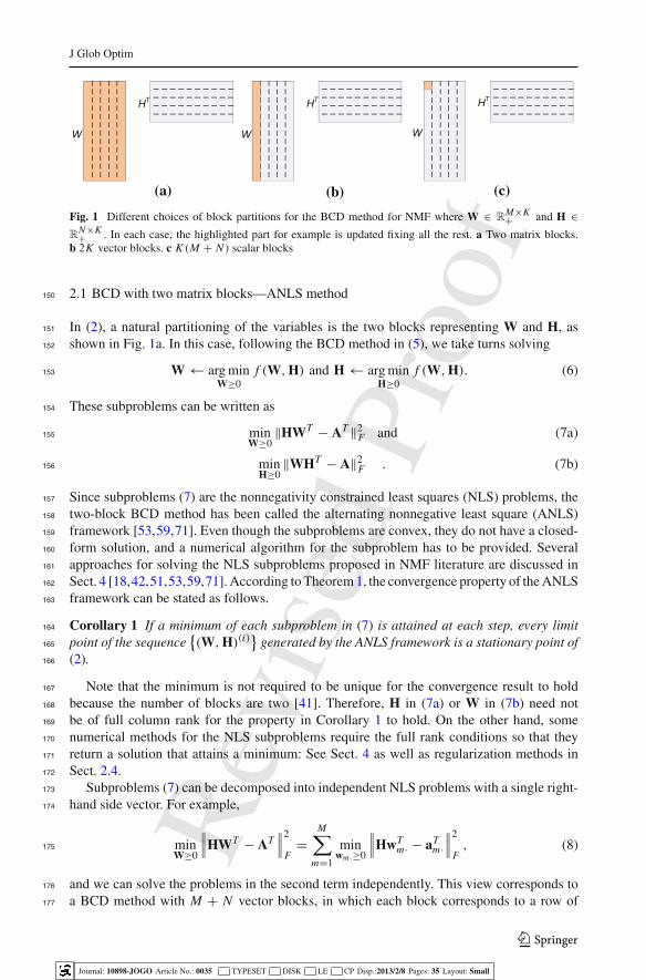
Fig. 1 Different choices of block partitions for the BCD method for NMF where W ∈ RM×K+ and H ∈

RN×K+ . In each case, the highlighted part for example is updated fixing all the rest. a Two matrix blocks.

b 2K vector blocks. c K (M + N ) scalar blocks

2.1 BCD with two matrix blocks—ANLS method150

In (2), a natural partitioning of the variables is the two blocks representing W and H, as151

shown in Fig. 1a. In this case, following the BCD method in (5), we take turns solving152

W← arg minW≥0

f (W,H) and H← arg minH≥0

f (W,H). (6)153

These subproblems can be written as154

minW≥0‖HWT − AT ‖2F and (7a)155

minH≥0‖WHT − A‖2F . (7b)156

Since subproblems (7) are the nonnegativity constrained least squares (NLS) problems, the157

two-block BCD method has been called the alternating nonnegative least square (ANLS)158

framework [53,59,71]. Even though the subproblems are convex, they do not have a closed-159

form solution, and a numerical algorithm for the subproblem has to be provided. Several160

approaches for solving the NLS subproblems proposed in NMF literature are discussed in161

Sect. 4 [18,42,51,53,59,71]. According to Theorem 1, the convergence property of the ANLS162

framework can be stated as follows.163

Corollary 1 If a minimum of each subproblem in (7) is attained at each step, every limit164

point of the sequence{(W,H)(i)

}generated by the ANLS framework is a stationary point of165

(2).166

Note that the minimum is not required to be unique for the convergence result to hold167

because the number of blocks are two [41]. Therefore, H in (7a) or W in (7b) need not168

be of full column rank for the property in Corollary 1 to hold. On the other hand, some169

numerical methods for the NLS subproblems require the full rank conditions so that they170

return a solution that attains a minimum: See Sect. 4 as well as regularization methods in171

Sect. 2.4.172

Subproblems (7) can be decomposed into independent NLS problems with a single right-173

hand side vector. For example,174

minW≥0

∥∥∥HWT − AT

∥∥∥

2

F=

M∑

m=1

minwm·≥0

∥∥∥HwT

m· − aTm·∥∥∥

2

F, (8)175

and we can solve the problems in the second term independently. This view corresponds to176

a BCD method with M + N vector blocks, in which each block corresponds to a row of177

123


Rev

ised

Proo

f

J Glob Optim

W or H. In literature, however, this view has not been emphasized because often it is more178

efficient to solve the NLS problems with multiple right-hand sides altogether: See Sect. 4.179

2.2 BCD with 2K vector blocks—HALS/RRI method180

Let us now partition the unknowns into 2K blocks in which each block is a column of181

W or H, as shown in Fig. 1b. In this case, it is easier to consider the objective function in the182

following form:183

f (w1, . . . ,wK ,h1, . . . ,hK ) =∥∥∥∥∥

A−K∑

k=1

wkhTk

∥∥∥∥∥

2

F

, (9)184

where W = [w1, . . .wK ] ∈ RM×K+ and H = [h1, . . . ,hK ] ∈ R

N×K+ . The form in (9)185

represents that A is approximated by the sum of K rank-one matrices.186

Following the BCD scheme, we can minimize f by iteratively solving187

wk ← arg minwk≥0

f (w1, . . . ,wK ,h1, . . . ,hK )188

for k = 1, . . . , K , and189

hk ← arg minhk≥0

f (w1, . . . ,wK ,h1, . . . ,hK )190

for k = 1, . . . , K . These subproblems appear as191

minw≥0‖hkwT − RT

k ‖2F and minh≥0‖wkhT − Rk‖2F , (10)192

where193

Rk = A−K∑

k=1,k �=k

wkhTk. (11)194

A promising aspect of this 2K block partitioning is that each subproblem in (10) has a195

closed-form solution, as characterized in the following theorem.196

Theorem 2 Consider a minimization problem197

minv≥0‖uvT −G‖2F (12)198

where G ∈ RM×N and u ∈ R

M are given. If u is a nonzero vector, v = [GT u]+uT u

is the unique199

solution for (12), where ([GT u]+)n = max((GT u)n, 0) for n = 1, . . . , N.200

Proof Letting vT = (v1, . . . , vN ), we have201

minv≥0

∥∥∥uvT −G

∥∥∥

2

F=

N∑

n=1

minvn≥0‖uvn − gn‖22 ,202

where G = [g1, . . . , gN ], and the problems in the second term are independent of each other.203

Let h(vn) = ‖uvn − gn‖22 = ‖u‖22v2n − 2vnuT gn + ‖gn‖22. Since ∂h

∂vn= 2(vn‖u‖22 − gT

n u),204

if gTn u ≥ 0, it is clear that the minimum value of h(vn) is attained at vn = gT

n uuT u

. If gTn u < 0,205

the value of h(vn) increases as vn becomes larger than zero, and therefore the minimum is206

attained at vn = 0. Combining the two cases, the solution can be expressed as vn = [gTn u]+uT u

.207

�208

123


Rev

ised

Proo

f

J Glob Optim

Using Theorem 2, the solutions of (10) can be stated as209

wk ← [Rkhk]+‖hk‖22

and hk ← [RTk wk]+‖wk‖22

. (13)210

This 2K -block BCD algorithm has been studied under the name of the hierarchical alternating211

least squares (HALS) method by Cichocki et al. [19,20] and the rank-one residue iteration212

(RRI) independently by Ho [44]. According to Theorem 1, the convergence property of the213

HALS/RRI algorithm can be written as follows.214

Corollary 2 If the columns of W and H remain nonzero throughout all the iterations and215

the minimums in (13) are attained at each step, every limit point of the sequence{(W,H)(i)

}216

generated by the HALS/RRI algorithm is a stationary point of (2).217

In practice, a zero column could occur in W or H during the HALS/RRI algorithm. This218

happens if hk ∈ null(Rk),wk ∈ null(RTk ),Rkhk ≤ 0, or RT

k wk ≤ 0. To prevent zero219

columns, a small positive number could be used for the maximum operator in (13): That is,220

max(·, ε) with a small positive number ε such as 10−16 is used instead of max(·, 0) [20,35].221

The HALS/RRI algorithm with this modification often shows faster convergence compared to222

other BCD methods or previously developed methods [37,59]. See Sect. 3.1 for acceleration223

techniques for the HALS/RRI method and Sect. 6.2 for more discussion on experimental224

comparisons.225

For an efficient implementation, it is not necessary to explicitly compute Rk . Replacing226

Rk in (13) with the expression in (11), the solutions can be rewritten as227

wk ←[wk + (AH)·k−(WHT H)·k

(HT H)kk

]

+ and (14a)228

hk ←[hk + (AT W)·k−(HWT W)·k

(WT W)kk

]

+ . (14b)229

The choice of update formulae is related with the choice of an update order. Two versions of230

an update order can be considered:231

w1 → h1 → · · · → wK → hK (15)232

and233

w1 → · · · → wK → h1 → · · · → hK . (16)234

When using (13), update order (15) is more efficient because Rk is explicitly computed and235

then used to update both wk and hk . When using (14), although either (15) or (16) can be used,236

update order (16) tends to be more efficient in environments such as MATLAB based on our237

experience. To update all the elements in W and H, update formulae (13) with ordering (15)238

require 8K M N +3K (M+ N ) floating point operations, whereas update formulae (14) with239

either choice of ordering require 4K M N + (4K 2 + 6K )(M + N ) floating point operations.240

When K � min(M, N ), the latter is more efficient. Moreover, the memory requirement of241

(14) is smaller because Rk need not be stored. For more details, see Cichocki and Phan [19].242

2.3 BCD with K (M + N ) scalar blocks243

In one extreme, the unknowns can be partitioned into K (M+ N ) blocks of scalars, as shown244

in Fig. 1c. In this case, every element of W and H is considered as a block in the context245

123


Rev

ised

Proo

f

J Glob Optim

of Theorem 1. To this end, it helps to write the objective function as a quadratic function of246

scalar wmk or hnk assuming all other elements in W and H are fixed:247

f (wmk) =∥∥∥∥∥∥

⎛

⎝am· −∑

k �=k

wmkhT·k

⎞

⎠− wmkhT·k

∥∥∥∥∥∥

2

2

+ const, (17a)248

f (hnk) =∥∥∥∥∥∥

⎛

⎝a·n −∑

k �=k

w·k hnk

⎞

⎠− w·khnk

∥∥∥∥∥∥

2

2

+ const, (17b)249

where am· and a·n denote the mth row and the nth column of A, respectively. According to250

the BCD framework, we iteratively update each block by251

wmk ← arg minwmk≥0

f (wmk) =[

wmk + (AH)mk − (WHT H)mk

(HT H)kk

]

+(18a)252

hnk ← arg minhnk≥0

f (hnk) =[

hnk + (AT W)nk − (HWT W)nk

(WT W)kk

]

+. (18b)253

The updates of wmk and hnk are independent of all other elements in the same column.254

Therefore, it is possible to update all the elements in each column of W (and H) simulta-255

neously. Once we organize the update of (18) column-wise, the result is the same as (14).256

That is, a particular arrangement of the BCD method with scalar blocks is equivalent to the257

BCD method with 2K vector blocks. Accordingly, the HALS/RRI method can be derived258

by the BCD method either with vector blocks or with scalar blocks. On the other hand, it is259

not possible to simultaneously solve for the elements in each row of W (or H) because their260

solutions depend on each other. The convergence property of the scalar block case is similar261

to that of the vector block case.262

Corollary 3 If the columns of W and H remain nonzero throughout all the iterations and if263

the minimums in (18) are attained at each step, every limit point of the sequence{(W,H)(i)

}264

generated by the BCD method with K (M + N ) scalar blocks is a stationary point of (2).265

The multiplicative updating rule also uses element-wise updating [67]. However, the266

multiplicative updating rule is different from the scalar block BCD method in a sense that its267

solutions are not optimal for subproblems (18). See Sect. 3.2 for more discussion.268

2.4 BCD for some variants of NMF269

To incorporate extra constraints or prior information into the NMF formulation in (2), various270

regularization terms can be added. We can consider an objective function271

minW,H≥0

∥∥∥A−WHT

∥∥∥

2

F+ φ(W)+ ψ(H), (19)272

where φ(·) and ψ(·) are regularization terms that often involve matrix or vector norms.273

Here we discuss the Frobenius-norm and the l1-norm regularization and show how NMF274

regularized by those norms can be easily computed using the BCD method. Scalar parameters275

α or β in this subsection are used to control the strength of regularization.276

The Frobenius-norm regularization [53,76] corresponds to277

φ(W) = α‖W‖2F and ψ(H) = β ‖H‖2F . (20)278

123


Rev

ised

Proo

f

J Glob Optim

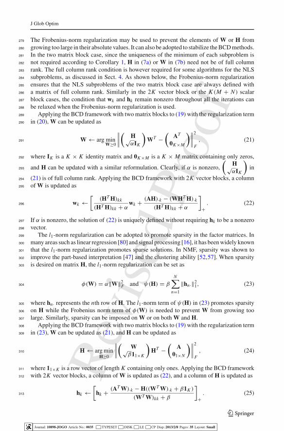
The Frobenius-norm regularization may be used to prevent the elements of W or H from279

growing too large in their absolute values. It can also be adopted to stabilize the BCD methods.280

In the two matrix block case, since the uniqueness of the minimum of each subproblem is281

not required according to Corollary 1, H in (7a) or W in (7b) need not be of full column282

rank. The full column rank condition is however required for some algorithms for the NLS283

subproblems, as discussed in Sect. 4. As shown below, the Frobenius-norm regularization284

ensures that the NLS subproblems of the two matrix block case are always defined with285

a matrix of full column rank. Similarly in the 2K vector block or the K (M + N ) scalar286

block cases, the condition that wk and hk remain nonzero throughout all the iterations can287

be relaxed when the Frobenius-norm regularization is used.288

Applying the BCD framework with two matrix blocks to (19) with the regularization term289

in (20), W can be updated as290

W← arg minW≥0

∥∥∥∥

(H√αIK

)WT −

(AT

0K×M

)∥∥∥∥

2

F, (21)291

where IK is a K × K identity matrix and 0K×M is a K × M matrix containing only zeros,292

and H can be updated with a similar reformulation. Clearly, if α is nonzero,

(H√αIK

)in293

(21) is of full column rank. Applying the BCD framework with 2K vector blocks, a column294

of W is updated as295

wk ←[

(HT H)kk

(HT H)kk + αwk + (AH)·k − (WHT H)·k(HT H)kk + α

]

+. (22)296

If α is nonzero, the solution of (22) is uniquely defined without requiring hk to be a nonzero297

vector.298

The l1-norm regularization can be adopted to promote sparsity in the factor matrices. In299

many areas such as linear regression [80] and signal processing [16], it has been widely known300

that the l1-norm regularization promotes sparse solutions. In NMF, sparsity was shown to301

improve the part-based interpretation [47] and the clustering ability [52,57]. When sparsity302

is desired on matrix H, the l1-norm regularization can be set as303

φ(W) = α‖W‖2F and ψ(H) = βN∑

n=1

‖hn·‖21, (23)304

where hn· represents the nth row of H. The l1-norm term of ψ(H) in (23) promotes sparsity305

on H while the Frobenius norm term of φ(W) is needed to prevent W from growing too306

large. Similarly, sparsity can be imposed on W or on both W and H.307

Applying the BCD framework with two matrix blocks to (19) with the regularization term308

in (23), W can be updated as (21), and H can be updated as309

H← arg minH≥0

∥∥∥∥

(W√β11×K

)HT −

(A

01×N

)∥∥∥∥

2

F, (24)310

where 11×K is a row vector of length K containing only ones. Applying the BCD framework311

with 2K vector blocks, a column of W is updated as (22), and a column of H is updated as312

hk ←[

hk + (AT W)·k −H((WT W)·k + β1K )

(WT W)kk + β]

+. (25)313

123


Rev

ised

Proo

f

J Glob Optim

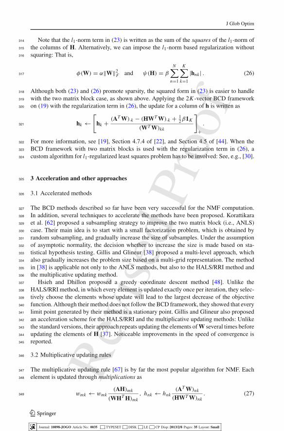
Note that the l1-norm term in (23) is written as the sum of the squares of the l1-norm of314

the columns of H. Alternatively, we can impose the l1-norm based regularization without315

squaring: That is,316

φ(W) = α‖W‖2F and ψ(H) = βN∑

n=1

K∑

k=1

|hnk | . (26)317

Although both (23) and (26) promote sparsity, the squared form in (23) is easier to handle318

with the two matrix block case, as shown above. Applying the 2K -vector BCD framework319

on (19) with the regularization term in (26), the update for a column of h is written as320

hk ←[

hk + (AT W)·k − (HWT W)·k + 1

2β1K

(WT W)kk

]

+.321

For more information, see [19], Section 4.7.4 of [22], and Section 4.5 of [44]. When the322

BCD framework with two matrix blocks is used with the regularization term in (26), a323

custom algorithm for l1-regularized least squares problem has to be involved: See, e.g., [30].324

3 Acceleration and other approaches325

3.1 Accelerated methods326

The BCD methods described so far have been very successful for the NMF computation.327

In addition, several techniques to accelerate the methods have been proposed. Korattikara328

et al. [62] proposed a subsampling strategy to improve the two matrix block (i.e., ANLS)329

case. Their main idea is to start with a small factorization problem, which is obtained by330

random subsampling, and gradually increase the size of subsamples. Under the assumption331

of asymptotic normality, the decision whether to increase the size is made based on sta-332

tistical hypothesis testing. Gillis and Glineur [38] proposed a multi-level approach, which333

also gradually increases the problem size based on a multi-grid representation. The method334

in [38] is applicable not only to the ANLS methods, but also to the HALS/RRI method and335

the multiplicative updating method.336

Hsieh and Dhillon proposed a greedy coordinate descent method [48]. Unlike the337

HALS/RRI method, in which every element is updated exactly once per iteration, they selec-338

tively choose the elements whose update will lead to the largest decrease of the objective339

function. Although their method does not follow the BCD framework, they showed that every340

limit point generated by their method is a stationary point. Gillis and Glineur also proposed341

an acceleration scheme for the HALS/RRI and the multiplicative updating methods: Unlike342

the standard versions, their approach repeats updating the elements of W several times before343

updating the elements of H [37]. Noticeable improvements in the speed of convergence is344

reported.345

3.2 Multiplicative updating rules346

The multiplicative updating rule [67] is by far the most popular algorithm for NMF. Each347

element is updated through multiplications as348

wmk ← wmk(AH)mk

(WHT H)mk, hnk ← hnk

(AT W)nk

(HWT W)nk. (27)349

123


Rev

ised

Proo

f

J Glob Optim

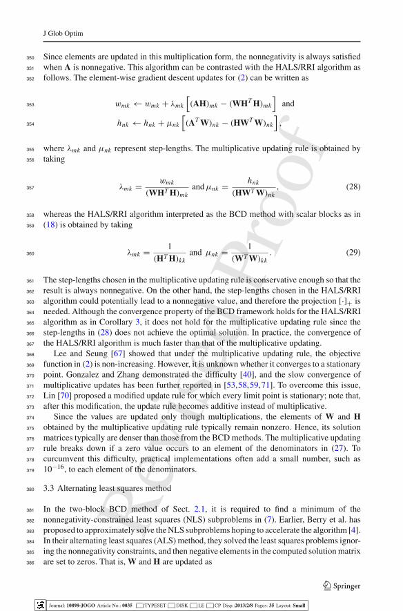
Since elements are updated in this multiplication form, the nonnegativity is always satisfied350

when A is nonnegative. This algorithm can be contrasted with the HALS/RRI algorithm as351

follows. The element-wise gradient descent updates for (2) can be written as352

wmk ← wmk + λmk

[(AH)mk − (WHT H)mk

]and353

hnk ← hnk + μnk

[(AT W)nk − (HWT W)nk

],354

where λmk and μnk represent step-lengths. The multiplicative updating rule is obtained by355

taking356

λmk = wmk

(WHT H)mkandμnk = hnk

(HWT W)nk, (28)357

whereas the HALS/RRI algorithm interpreted as the BCD method with scalar blocks as in358

(18) is obtained by taking359

λmk = 1

(HT H)kkand μnk = 1

(WT W)kk. (29)360

The step-lengths chosen in the multiplicative updating rule is conservative enough so that the361

result is always nonnegative. On the other hand, the step-lengths chosen in the HALS/RRI362

algorithm could potentially lead to a nonnegative value, and therefore the projection [·]+ is363

needed. Although the convergence property of the BCD framework holds for the HALS/RRI364

algorithm as in Corollary 3, it does not hold for the multiplicative updating rule since the365

step-lengths in (28) does not achieve the optimal solution. In practice, the convergence of366

the HALS/RRI algorithm is much faster than that of the multiplicative updating.367

Lee and Seung [67] showed that under the multiplicative updating rule, the objective368

function in (2) is non-increasing. However, it is unknown whether it converges to a stationary369

point. Gonzalez and Zhang demonstrated the difficulty [40], and the slow convergence of370

multiplicative updates has been further reported in [53,58,59,71]. To overcome this issue,371

Lin [70] proposed a modified update rule for which every limit point is stationary; note that,372

after this modification, the update rule becomes additive instead of multiplicative.373

Since the values are updated only though multiplications, the elements of W and H374

obtained by the multiplicative updating rule typically remain nonzero. Hence, its solution375

matrices typically are denser than those from the BCD methods. The multiplicative updating376

rule breaks down if a zero value occurs to an element of the denominators in (27). To377

curcumvent this difficulty, practical implementations often add a small number, such as378

10−16, to each element of the denominators.379

3.3 Alternating least squares method380

In the two-block BCD method of Sect. 2.1, it is required to find a minimum of the381

nonnegativity-constrained least squares (NLS) subproblems in (7). Earlier, Berry et al. has382

proposed to approximately solve the NLS subproblems hoping to accelerate the algorithm [4].383

In their alternating least squares (ALS) method, they solved the least squares problems ignor-384

ing the nonnegativity constraints, and then negative elements in the computed solution matrix385

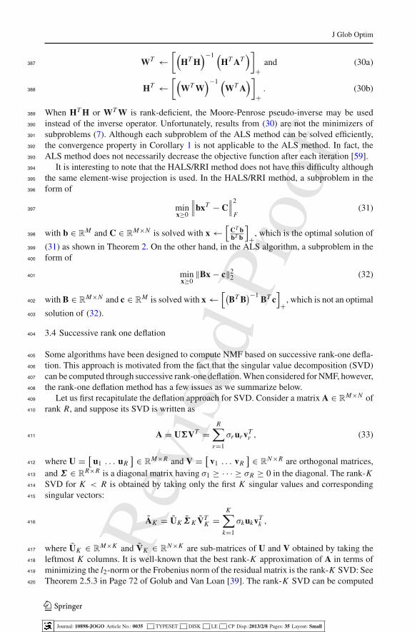
are set to zeros. That is, W and H are updated as386

123


Rev

ised

Proo

f

J Glob Optim

WT ←[(

HT H)−1 (

HT AT)]

+and (30a)387

HT ←[(

WT W)−1 (

WT A)]

+. (30b)388

When HT H or WT W is rank-deficient, the Moore-Penrose pseudo-inverse may be used389

instead of the inverse operator. Unfortunately, results from (30) are not the minimizers of390

subproblems (7). Although each subproblem of the ALS method can be solved efficiently,391

the convergence property in Corollary 1 is not applicable to the ALS method. In fact, the392

ALS method does not necessarily decrease the objective function after each iteration [59].393

It is interesting to note that the HALS/RRI method does not have this difficulty although394

the same element-wise projection is used. In the HALS/RRI method, a subproblem in the395

form of396

minx≥0

∥∥∥bxT − C

∥∥∥

2

F(31)397

with b ∈ RM and C ∈ R

M×N is solved with x←[

CT bbT b

]

+, which is the optimal solution of398

(31) as shown in Theorem 2. On the other hand, in the ALS algorithm, a subproblem in the399

form of400

minx≥0‖Bx − c‖22 (32)401

with B ∈ RM×N and c ∈ R

M is solved with x←[(

BT B)−1

BT c]

+, which is not an optimal402

solution of (32).403

3.4 Successive rank one deflation404

Some algorithms have been designed to compute NMF based on successive rank-one defla-405

tion. This approach is motivated from the fact that the singular value decomposition (SVD)406

can be computed through successive rank-one deflation. When considered for NMF, however,407

the rank-one deflation method has a few issues as we summarize below.408

Let us first recapitulate the deflation approach for SVD. Consider a matrix A ∈ RM×N of409

rank R, and suppose its SVD is written as410

A = U�VT =R∑

r=1

σr ur vTr , (33)411

where U = [u1 . . . uR] ∈ R

M×R and V = [ v1 . . . vR] ∈ R

N×R are orthogonal matrices,412

and Σ ∈ RR×R is a diagonal matrix having σ1 ≥ · · · ≥ σR ≥ 0 in the diagonal. The rank-K413

SVD for K < R is obtained by taking only the first K singular values and corresponding414

singular vectors:415

AK = UK Σ K VTK =

K∑

k=1

σkukvTk ,416

where UK ∈ RM×K and VK ∈ R

N×K are sub-matrices of U and V obtained by taking the417

leftmost K columns. It is well-known that the best rank-K approximation of A in terms of418

minimizing the l2-norm or the Frobenius norm of the residual matrix is the rank-K SVD: See419

Theorem 2.5.3 in Page 72 of Golub and Van Loan [39]. The rank-K SVD can be computed420

123


Rev

ised

Proo

f

J Glob Optim

through successive rank one deflation as follows. First, the best rank-one approximation,421

σ1u1vT1 , is computed with an efficient algorithm such as the power iteration. Then, the422

residual matrix is obtained as E1 = A − σ1u1vT1 =

∑Rr=2 σr ur vT

r , and the rank of E1 is423

R − 1. For the residual matrix E1, its best rank-one approximation, σ2u2vT2 , is obtained,424

and the residual matrix E2, whose rank is R − 2, can be found in the same manner: E2 =425

E1−σ2u2vT2 =

∑Rr=3 σr ur vT

r . Repeating this process for K times, one can obtain the rank-K426

SVD.427

When it comes to NMF, a notable theoretical result about nonnegative matrices relates428

SVD and NMF when K = 1. The following theorem, which extends the Perron-Frobenius429

theorem [3,45], is shown in Chapter 2 of Berman and Plemmons [3].430

Theorem 3 For a nonnegative symmetric matrix A ∈ RN×N+ , the eigenvalue of A with the431

largest magnitude is nonnegative, and there exists a nonnegative eigenvector corresponding432

to the largest eigenvalue.433

A direct consequence of Theorem 3 is the nonnegativity of the best rank-one approxima-434

tion.435

Corollary 4 (Nonnegativity of best rank-one approximation) For any nonnegative matrix436

A ∈ RM×N+ , the following minimization problem437

minu∈RM ,v∈RN

∥∥∥A− uvT

∥∥∥

2

F. (34)438

has an optimal solution satisfying u ≥ 0 and v ≥ 0.439

Another way to realizing Corollary 4 is through the use of the SVD. For a nonnegative440

matrix A ∈ RM×N+ and for any vectors u ∈ R

M and v ∈ RN ,441

∥∥∥A− uvT

∥∥∥

2

F=

M∑

m=1

N∑

n=1

(amn − umvn)2

442

≥M∑

m=1

N∑

n=1

(amn − |um | |vn |)2 . (35)443

Hence, element-wise absolute values can be taken from the left and right singular vectors that444

correspond to the largest singular value to achieve the best rank-one approximation satisfying445

nonnegativity. There might be other optimal solutions of (34) involving negative numbers:446

See [34].447

The elegant property in Corollary 4, however, is not readily applicable when K ≥ 2. After448

the best rank-one approximation matrix is deflated, the residual matrix may contain negative449

elements, and then Corollary 4 is not applicable any more. In general, successive rank-one450

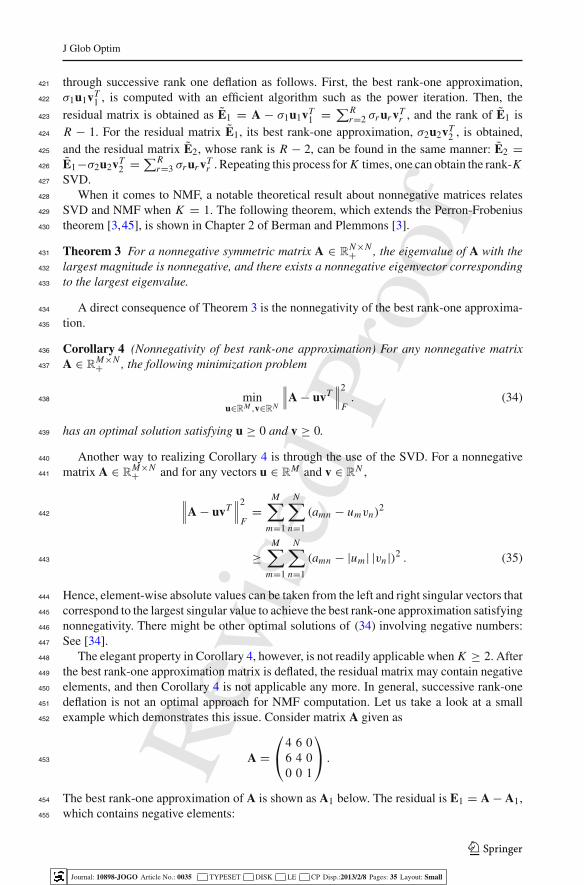
deflation is not an optimal approach for NMF computation. Let us take a look at a small451

example which demonstrates this issue. Consider matrix A given as452

A =⎛

⎝4 6 06 4 00 0 1

⎞

⎠ .453

The best rank-one approximation of A is shown as A1 below. The residual is E1 = A−A1,454

which contains negative elements:455

123


Rev

ised

Proo

f

J Glob Optim

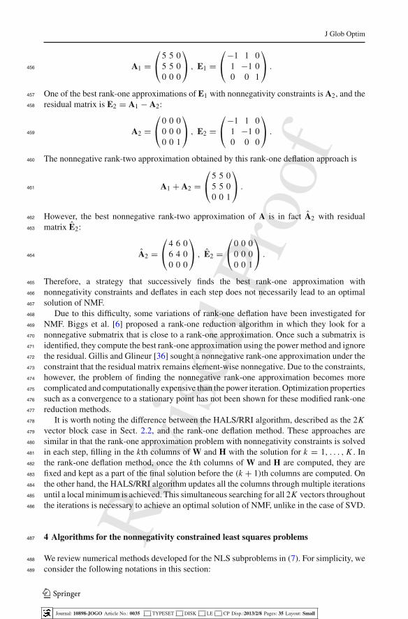
A1 =⎛

⎝5 5 05 5 00 0 0

⎞

⎠ , E1 =⎛

⎝−1 1 01 −1 00 0 1

⎞

⎠ .456

One of the best rank-one approximations of E1 with nonnegativity constraints is A2, and the457

residual matrix is E2 = A1 − A2:458

A2 =⎛

⎝0 0 00 0 00 0 1

⎞

⎠ , E2 =⎛

⎝−1 1 01 −1 00 0 0

⎞

⎠ .459

The nonnegative rank-two approximation obtained by this rank-one deflation approach is460

A1 + A2 =⎛

⎝5 5 05 5 00 0 1

⎞

⎠ .461

However, the best nonnegative rank-two approximation of A is in fact A2 with residual462

matrix E2:463

A2 =⎛

⎝4 6 06 4 00 0 0

⎞

⎠ , E2 =⎛

⎝0 0 00 0 00 0 1

⎞

⎠ .464

Therefore, a strategy that successively finds the best rank-one approximation with465

nonnegativity constraints and deflates in each step does not necessarily lead to an optimal466

solution of NMF.467

Due to this difficulty, some variations of rank-one deflation have been investigated for468

NMF. Biggs et al. [6] proposed a rank-one reduction algorithm in which they look for a469

nonnegative submatrix that is close to a rank-one approximation. Once such a submatrix is470

identified, they compute the best rank-one approximation using the power method and ignore471

the residual. Gillis and Glineur [36] sought a nonnegative rank-one approximation under the472

constraint that the residual matrix remains element-wise nonnegative. Due to the constraints,473

however, the problem of finding the nonnegative rank-one approximation becomes more474

complicated and computationally expensive than the power iteration. Optimization properties475

such as a convergence to a stationary point has not been shown for these modified rank-one476

reduction methods.477

It is worth noting the difference between the HALS/RRI algorithm, described as the 2K478

vector block case in Sect. 2.2, and the rank-one deflation method. These approaches are479

similar in that the rank-one approximation problem with nonnegativity constraints is solved480

in each step, filling in the kth columns of W and H with the solution for k = 1, . . . , K . In481

the rank-one deflation method, once the kth columns of W and H are computed, they are482

fixed and kept as a part of the final solution before the (k + 1)th columns are computed. On483

the other hand, the HALS/RRI algorithm updates all the columns through multiple iterations484

until a local minimum is achieved. This simultaneous searching for all 2K vectors throughout485

the iterations is necessary to achieve an optimal solution of NMF, unlike in the case of SVD.486

4 Algorithms for the nonnegativity constrained least squares problems487

We review numerical methods developed for the NLS subproblems in (7). For simplicity, we488

consider the following notations in this section:489

123


Rev

ised

Proo

f

J Glob Optim

minX≥0‖BX− C‖2F =

R∑

r=1

‖Bxr − cr‖22 , (36)490

where B ∈ RP×Q,C = [c1, . . . , cR] ∈ R

Q×R , and X = [x1, . . . , xR] ∈ RQ×R . We mainly491

discuss two groups of algorithms for the NLS problems. The first group consists of the492

gradient descent and the Newton-type methods that are modified to satisfy the nonnegativity493

constraints using a projection operator. The second group consists of the active-set and the494

active-set-like methods, in which zero and nonzero variables are explicitly kept track of and495

a system of linear equations is solved at each iteration. For more details, see Lawson and496

Hanson [64], Bjork [8], and Chen and Plemmons [15].497

To facilitate our discussion, we state a simple NLS problem with a single right-hand side:498

minx≥0

g(x) = ‖Bx − c‖22. (37)499

Problem (36) may be solved by handling independent problems for the columns of X, whose500

form appears as (37). Otherwise, the problem in (36) can also be transformed into501

minx1,...,xR≥0

∥∥∥∥∥∥∥

⎛

⎜⎝

B. . .

B

⎞

⎟⎠

⎛

⎜⎝

x1...

xR

⎞

⎟⎠−

⎛

⎜⎝

c1...

cR

⎞

⎟⎠

∥∥∥∥∥∥∥

2

2

. (38)502

4.1 Projected iterative methods503

Projected iterative methods for the NLS problems are designed based on the fact that the504

objective function in (36) is differentiable and that the projection to the nonnegative orthant505

is easy to compute. The first method of this type proposed for NMF was the projected gradient506

method of Lin [71]. Their update formula is written as507

x(i+1) ←[x(i) − α(i)∇g(x(i))

]

+ , (39)508

where x(i) and α(i) represent the variables and the step length at the i th iteration. Step length509

α(i) is chosen by a back-tracking line search to satisfy Armijo’s rule with an optional stage510

that increases the step length. Kim et al. [51] proposed a quasi-Newton method by utilizing511

the second order information to improve convergence:512

x(i+1) ←([

y(i) − α(i)D(i)∇g(y(i))]+

0

), (40)513

where y(i) is a subvector of x(i) with elements that are not optimal in terms of the Karush–514

Kuhn–Tucker (KKT) conditions. They efficiently updated D(i) using the BFGS method and515

selected α(i) by a back-tracking line search. Whereas Lin considered a stacked-up problem516

as in (38), the quasi-Newton method by Kim et al. was applied to each column separately.517

A notable variant of the projected gradient method is the Barzilai-Borwein method [7].518

Han et al. [42] proposed alternating projected Barzilai-Borwein method for NMF. A key519

characteristic of the Barzilai-Borwein method in unconstrained quadratic programming is520

that the step-length is chosen by a closed-form formula without having to perform a line521

search:522

x(i+1) ←[x(i) − α(i)∇g(x(i))

]

+ with α(i) = sT syT s

, where523

s = x(i) − x(i−1) and y = ∇g(x(i))− ∇g(x(i−1)).524

123


Rev

ised

Proo

f

J Glob Optim

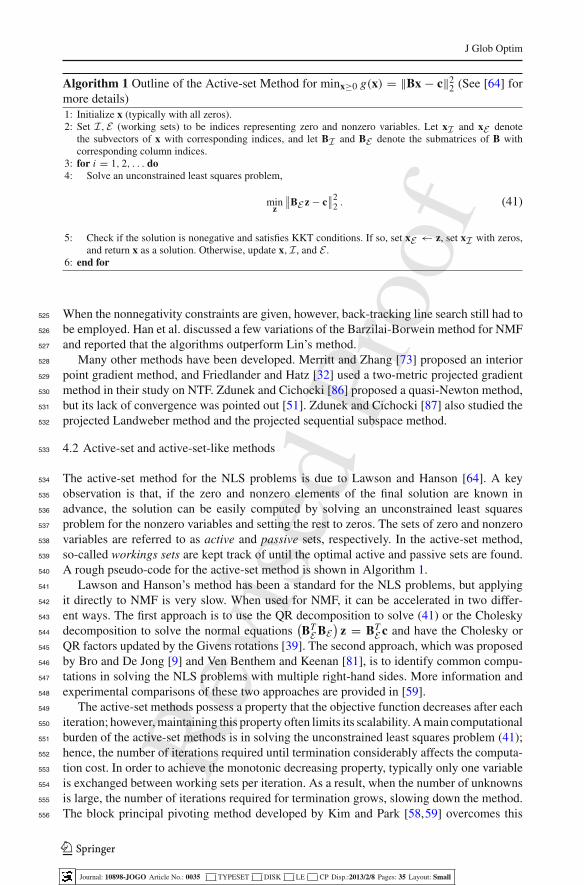
Algorithm 1 Outline of the Active-set Method for minx≥0 g(x) = ‖Bx − c‖22 (See [64] formore details)1: Initialize x (typically with all zeros).2: Set I,E (working sets) to be indices representing zero and nonzero variables. Let xI and xE denote

the subvectors of x with corresponding indices, and let BI and BE denote the submatrices of B withcorresponding column indices.

3: for i = 1, 2, . . . do4: Solve an unconstrained least squares problem,

minz

∥∥BE z− c

∥∥2

2 . (41)

5: Check if the solution is nonegative and satisfies KKT conditions. If so, set xE ← z, set xI with zeros,and return x as a solution. Otherwise, update x,I, and E .

6: end for

When the nonnegativity constraints are given, however, back-tracking line search still had to525

be employed. Han et al. discussed a few variations of the Barzilai-Borwein method for NMF526

and reported that the algorithms outperform Lin’s method.527

Many other methods have been developed. Merritt and Zhang [73] proposed an interior528

point gradient method, and Friedlander and Hatz [32] used a two-metric projected gradient529

method in their study on NTF. Zdunek and Cichocki [86] proposed a quasi-Newton method,530

but its lack of convergence was pointed out [51]. Zdunek and Cichocki [87] also studied the531

projected Landweber method and the projected sequential subspace method.532

4.2 Active-set and active-set-like methods533

The active-set method for the NLS problems is due to Lawson and Hanson [64]. A key534

observation is that, if the zero and nonzero elements of the final solution are known in535

advance, the solution can be easily computed by solving an unconstrained least squares536

problem for the nonzero variables and setting the rest to zeros. The sets of zero and nonzero537

variables are referred to as active and passive sets, respectively. In the active-set method,538

so-called workings sets are kept track of until the optimal active and passive sets are found.539

A rough pseudo-code for the active-set method is shown in Algorithm 1.540

Lawson and Hanson’s method has been a standard for the NLS problems, but applying541

it directly to NMF is very slow. When used for NMF, it can be accelerated in two differ-542

ent ways. The first approach is to use the QR decomposition to solve (41) or the Cholesky543

decomposition to solve the normal equations(BT

E BE)

z = BTE c and have the Cholesky or544

QR factors updated by the Givens rotations [39]. The second approach, which was proposed545

by Bro and De Jong [9] and Ven Benthem and Keenan [81], is to identify common compu-546

tations in solving the NLS problems with multiple right-hand sides. More information and547

experimental comparisons of these two approaches are provided in [59].548

The active-set methods possess a property that the objective function decreases after each549

iteration; however, maintaining this property often limits its scalability. A main computational550

burden of the active-set methods is in solving the unconstrained least squares problem (41);551

hence, the number of iterations required until termination considerably affects the computa-552

tion cost. In order to achieve the monotonic decreasing property, typically only one variable553

is exchanged between working sets per iteration. As a result, when the number of unknowns554

is large, the number of iterations required for termination grows, slowing down the method.555

The block principal pivoting method developed by Kim and Park [58,59] overcomes this556

123


Rev

ised

Proo

f

J Glob Optim

limitation. Their method, which is based on the work of Judice and Pires [50], allows the557

exchanges of multiple variables between working sets. This method does not maintain the558

nonnegativity of intermediate vectors nor the monotonic decrease of the objective function,559

but it requires a smaller number of iterations until termination than the active set methods. It560

is worth emphasizing that the grouping-based speed-up technique, which was earlier devised561

for the active-set method, is also effective with the block principal pivoting method for the562

NMF computation: For more details, see [59].563

4.3 Discussion and other methods564

A main difference between the projected iterative methods and the active-set-like methods565

for the NLS problems lies in their convergence or termination. In projected iterative methods,566

a sequence of tentative solutions is generated so that an optimal solution is approached in567

the limit. In practice, one has to somehow stop iterations and return the current estimate,568

which might be only an approximation of the solution. In the active-set and active-set-like569

methods, in contrast, there is no concept of a limit point. Tentative solutions are generated570

with a goal of finding the optimal active and passive set partitioning, which is guaranteed571

to be found in a finite number of iterations since there are only a finite number of possible572

active and passive set partitionings. Once the optimal active and passive sets are found,573

the methods terminate. There are trade-offs of these behavior. While the projected iterative574

methods may return an approximate solution after a few number of iterations, the active-set575

and active-set-like methods only return a solution after they terminate. After the termination,576

however, the solution from the active-set-like methods is an exact solution only subject to577

numerical rounding errors while the solution from the projected iterative methods might be578

an approximate one.579

Other approaches for solving the NLS problems can be considered as a subroutine for the580

NMF computation. Bellavia et al. [2] have studied an interior point Newton-like method, and581

Franc et al. [31] presented a sequential coordinate-wise method. Some observations about the582

NMF computation based on these methods as well as other methods are offered in Cichocki583

et al. [22]. Chu and Lin [18] proposed an algorithm based on low-dimensional polytope584

approximation: Their algorithm is motivated by a geometrical interpretation of NMF that585

data points are approximated by a simplicial cone [27].586

Different conditions are required for the NLS algorithms to guarantee convergence or587

termination. The requirement of the projected gradient method [71] is mild as it only requires588

an appropriate selection of the step-length. Both the quasi-Newton method [51] and the589

interior point gradient method [73] require that matrix B in (37) is of full column rank. The590

active-set method [53,64] does not require the full-rank condition as long as a zero vector is591

used for initialization [28]. In the block principal pivoting method [58,59], on the other hand,592

the full-rank condition is required. Since NMF is formulated as a lower rank approximation593

and K is typically much smaller than the rank of the input matrix, the ranks of both W and H in594

(7) typically remain full. When this condition is not likely to be satisfied, the Frobenius-norm595

regularization of Sect. 2.4 can be adopted to guarantee the full rank condition.596

5 BCD framework for nonnegative CP597

Our discussion on the low-rank factorizations of nonnegative matrices naturally extends598

to those of nonnegative tensors. In this section, we discuss nonnegative CANDE-599

COMP/PARAFAC (NCP) and explain how it can be computed by the BCD framework.600

123


Rev

ised

Proo

f

J Glob Optim

A few other decomposition models of higher order tensors have been studied, and interested601

readers are referred to [1,61]. The organization of this section is similar to that of Sect. 2,602

and we will show that the NLS algorithms reviewed in Sect. 4 can also be used to factorize603

tensors.604

Let us consider an N th-order tensor A ∈ RM1×···×MN . For an integer K , we are605

interested in finding nonnegative factor matrices H(1), . . . ,H(N ) where H(n) ∈RMn×K for606

n = 1, . . . , N such that607

A ≈ [[H(1), . . . ,H(N )]], (42)608609

where610

H(n) =[

h(n)1 . . . h(n)K

]for n = 1, . . . , N and (43)611

612

613

[[H(1), . . . ,H(N )]] =K∑

k=1

h(1)k ◦ · · · ◦ h(N )k . (44)614

615

The ‘◦’ symbol represents the outer product of vectors, and a tensor in the form of616

h(1)k ◦· · ·◦h(N )k is called a rank-one tensor. Model (42) is known as CANDECOMP/PARAFAC617

(CP) [14,43]: In the CP decomposition, A is represented as the sum of K rank-one tensors.618

The smallest integer K for which (42) holds as equality is called the rank of tensor A. The619

CP decomposition reduces to a matrix decomposition if N = 2. The nonnegative CP decom-620

position is obtained by adding nonnegativity constraints to factor matrices H(1), . . . ,H(N ).621

A corresponding problem can be written as, for A ∈ RM1×···×MN+ ,622

minH(1),...,H(N )

f (H(1), . . . ,H(N )) =∥∥∥A − [[H(1), . . . ,H(N )]]

∥∥∥

2

F,623

624s.t. H(n) ≥ 0 for n = 1, . . . N . (45)625

626

We discuss algorithms for solving (45) in this section [19,32,54,60]. Toward that end, we627

introduce definitions of some operations of tensors.628

Mode-n matricization: The mode-n matricization of A ∈ RM1×···×MN , denoted by A<n>,629

is a matrix obtained by linearizing all the indices of tensor A except n. Specifically, A<n> is630

a matrix of size Mn × (∏Nn=1,n �=n Mn), and the (m1, . . . ,m N )th element of A is mapped to631

the (mn, J )th element of A<n> where632

J = 1+N∑

j=1

(m j − 1)J j and J j =j−1∏

l=1,l �=n

Ml .633

Mode-n fibers: The fibers of higher-order tensors are vectors obtained by specifying634

all indices except one. Given a tensor A ∈ RM1×···×MN , a mode-n fiber denoted by635

am1...mn−1:mn+1...m N is a vector of length Mn with all the elements having m1, . . . ,mn−1,636

mn+1, . . . ,m N as indices for the 1st, . . . , (n−1)th, (n+2)th, . . . , N th orders. The columns637

and the rows of a matrix are the mode-1 and the mode-2 fibers, respectively.638

Mode-n product: The mode-n product of a tensor A ∈ RM1×···×MN and a matrix U ∈639

RJ×Mn , denoted by A×n U, is a tensor obtained by multiplying all mode-n fibers of A with640

the columns of U. The result is a tensor of size M1 × · · · × Mn−1 × J × Mn+1 × · · · × MN641

having elements as642

(A×n U)m1...mn−1 jmn+1...m N=

Mn∑

mn=1

xm1...m N u jmn .643

123


Rev

ised

Proo

f

J Glob Optim

In particular, the mode-n product of A and a vector u ∈ RMn is a tensor of size M1 × · · · ×644

Mn−1 × Mn+1 × · · · × MN .645

Khatri-Rao product: The Khatri-Rao product of two matrices A ∈ RJ1×L and B ∈ R

J2×L ,646

denoted by A� B ∈ R(J1 J2)×L , is defined as647

A� B =

⎡

⎢⎢⎢⎣

a11b1 a12b2 · · · a1L bL

a21b1 a22b2 · · · a2L bL...

.... . .

...

aJ11b1 aJ12b2 · · · aJ1 L bL

⎤

⎥⎥⎥⎦.648

5.1 BCD with N matrix blocks649

A simple BCD method can be designed for (45) considering each of the factor matrics650

H(1), . . . ,H(N ) as a block. Using notations introduced above, approximation model (42) can651

be written as, for any n ∈ {1, . . . , N },652

A<n> ≈ H(n)(

B(n))T, (46)653

654

where655

B(n) = H(N ) � · · · �H(n+1) �H(n−1) � · · · �H(1)656

657 ∈ R

(∏Nn=1,n �=n Mn

)×K. (47)658

659

Representation in (46) simplifies the treatment of this N matrix block case. After660

H(2), . . . ,H(N ) are initialized with nonnegative elements, the following subproblem is solved661

iteratively for n = 1, . . . N :662

H(n) ← arg minH≥0

∥∥∥B(n)HT − (A<n>)T

∥∥∥

2

F. (48)663

664

Since subproblem (48) is an NLS problem, as in the matrix factorization case, this matrix-665

block BCD method is called the alternating nonnegative least squares (ANLS) framework666

[32,54,60]. The convergence property of the BCD method in Theorem 1 yields the following667

corollary.668

Corollary 5 If a unique solution exists for (48) and is attained for n = 1, . . . , N, then every669

limit point of the sequence{(

H(1), . . . ,H(N ))(i)}

generated by the ANLS framework is a670

stationary point of (45).671

In particular, if each B(n) is of full column rank, the subproblem has a unique solution.672

Algorithms for the NLS subproblems discussed in Sect. 4 can be used to solve (48).673

For higher order tensors, the number of rows in B(n) and (A<n>)T , i.e.,∏N

n=1,n �=n Mn , can674

be quite large. However, often B(n) and (A<n>)T do not need to be explicitly constructed. In675

most algorithms explained in Sect. 4, it is enough to have B(n)T (A<n>)T and(B(n)

)TB(n).676

It is easy to verify that B(n)T (A<n>)T can be obtained by successive mode-n products:677

B(n)T(A<n>)T = A×1 H(1) . . .×(n−1) H(n−1)

678

679 ×(n)H(n) . . .×(N ) H(N ). (49)680681

123


Rev

ised

Proo

f

J Glob Optim

In addition,(B(n)

)TB(n) can be obtained as682

(B(n)

)TB(n) =

N⊗

n=1,n �=n

(H(n)

)TH(n), (50)683

684

where⊗

represents element-wise multiplication.685

5.2 BCD with K N vector blocks686

Another way to apply the BCD framework to (45) is to treat each column of H(1), . . . ,H(N )687

as a block. The columns are updated by solving, for n = 1, . . . N and for k = 1, . . . , K ,688

h(n)k ←689

690

arg minh≥0

∥∥∥[[h(1)k , . . . ,h(n−1)

k ,h,h(n+1)k , · · · ,h(N )k ]] −Rk

∥∥∥

2

F. (51)691

692

where693

Rk = A −K∑

k=1,k �=k

h(1)k◦ · · · ◦ h(N )

k.694

Using matrix notations, problem (51) can be rewritten as695

h(n)k ← arg minh≥0

∥∥∥b(n)k hT − (R<n>

k

)T∥∥∥

2

F, (52)696

697

where R<n>k is the mode-n matricization of Rk and698

b(n)k = h(N )k � · · · � h(n+1)k � h(n−1)

k � · · · � h(1)k699

700

∈ R

(∏Nn=1,n �=n Mn

)×1. (53)701

702

This vector-block BCD method corresponds to the HALS method by Cichocki et al. for703

NTF [19,22]. The convergence property in Theorem 1 yields the following corollary.704

Corollary 6 If a unique solution exists for (52) and is attained for n = 1, . . . , N and for705

k = 1, . . . , K , every limit point of the sequence{(

H(1), . . . ,H(N ))(i)}

generated by the706

vector-block BCD method is a stationary point of (45).707

Using Theorem 2, the solution of (52) is708

h(n)k ←[R<n>

k b(n)k

]

+∥∥∥b(n)k

∥∥∥

2

2

. (54)709

710

Solution (54) can be evaluated without constructing R<n>k . Observe that711

(b(n)k

)Tb(n)k =

N∏

n=1,n �=n

(h(n)k

)Th(n)k , (55)712

713

123


Rev

ised

Proo

f

J Glob Optim

which is a simple case of (50), and714

R<n>k b(n)k =

⎛

⎝A −K∑

k=1,k �=k

h(1)k◦ · · · ◦ h(N )

k

⎞

⎠

<n>

b(n)k (56)715

716

717

= A<n>b(n)k −K∑

k=1,k �=k

⎛

⎝N∏

n=1,n �=n

(h(n)

k

)Th(n)k

⎞

⎠h(n)k. (57)718

719

Solution (54) can then be simplified as720

h(n)k ←721

722 ⎡

⎢⎣h(n)k +

A<n>b(n)k −H(n)(⊗N

n=1,n �=n

(H(n)

)TH(n)

)

·k∏N

n=1,n �=n

(h(n)k

)Th(n)k

⎤

⎥⎦ , (58)723

724

where A<n>b(n)k can be computed using (49). Observe the similarity between (58) and (14).725

6 Implementation issues and comparisons726

6.1 Stopping criterion727

Iterative methods have to be equipped with a criterion for stopping iterations. In NMF or728

NTF, an ideal criterion would be to stop iterations after a local minimum of (2) or (45) is729

attained. In practice, a few alternatives have been used.730

Let us first discuss stopping criteria for NMF. A naive approach is to stop when the decrease731

of the objective function becomes smaller than some predefined threshold:732

f (W(i−1),H(i−1))− f (W(i),H(i)) ≤ ε, (59)733734

where ε is a tolerance value to choose. Although this method is commonly adopted, it is735

potentially misleading because the decrease of the objective function may become small736

before a local minimum is achieved. A more principled criterion was proposed by Lin as fol-737

lows [71]. According to the Karush–Kuhn–Tucher (KKT) conditions, (W,H) is a stationary738

point of (2) if and only if [17]739

W ≥ 0, H ≥ 0, (60a)740741

742

∇ fW = ∂ f (W,H)∂W

≥ 0, ∇ fH = ∂ f (W,H)∂H

≥ 0, (60b)743744

745

W⊗∇ fW = 0, H

⊗∇ fH = 0, (60c)746747

where748

∇ fW = 2WHT H− 2AH and749

∇ fH = 2HWT W− 2AT W.750

123


Rev

ised

Proo

f

J Glob Optim

Define the projected gradient ∇ p fW ∈ RM×K as,751

(∇ p fW)

mk ≡{(∇ fW)mk if (∇ fW)mk < 0 or Wmk > 0,

0 otherwise,752

for m = 1, . . . ,M and k = 1, . . . , K , and ∇ p fH similarly. Then, conditions (60) can be753

rephrased as754

∇ p fW = 0 and ∇ p fH = 0.755

Denote the projected gradient matrices at the i th iteration by ∇ p f (i)W and ∇ p f (i)H , and define756

Δ(i) =√∥∥∥∇ p f (i)W

∥∥∥

2

F+∥∥∥∇ p f (i)H

∥∥∥

2

F. (61)757

758

Using this definition, the stopping criterion is written by759

Δ(i)

Δ(0)≤ ε, (62)760

761

whereΔ(0) is from the initial values of (W,H). Unlike (59), (62) guarantees the stationarity762

of the final solution. Variants of this criterion was used in [40,53].763

An analogous stopping criterion can be derived for the NCP formulation in (45).764

The gradient matrix ∇ fH(n) can be derived from the least squares representation in (48):765

∇ fH(n) = 2H(n)(

B(n))T

B(n) − 2A<n>B(n).766

See (49) and (50) for efficient computation of(B(n)

)TB(n) and A<n>B(n). With function Δ767

defined as768

Δ(i) =√√√√

N∑

n=1

∥∥∥∇ p f (i)

H(n)

∥∥∥

2

F, (63)769

770

criterion in (62) can be used to stop iterations of an NCP algorithm.771

Using (59) or (62) for the purpose of comparing algorithms might be unreliable. One might772

want to measure the amounts of time until several algorithms satisfy one of these criteria and773

compare them [53,71]. Such comparison would usually reveal meaningful trends, but there774

are some caveats. The difficulty of using (59) is straightforward because, in some algorithm775

such as the multiplicative updating rule, the difference in (59) can become quite small before776

arriving at a minimum. The difficulty of using (62) is as follows. Note that the diagonal777

rescaling of W and H does not affect the quality of approximation: For a diagonal matrix778

D ∈ RK×K+ with positive diagonal elements, WHT =WD−1 (HD)T . However, the norm of779

the projected gradients in (61) is affected by a diagonal scaling:780

(∂ f

∂(WD−1),

∂ f

∂(HD)

)=((

∂ f

∂W

)D,(∂ f

∂H

)D−1

).781

Hence, two solutions that are only different up to a diagonal scaling have the same objective782

function value, but they can be measured differently in terms of the norm of the projected783

gradients. See Kim and Park [59] for more information. Ho [44] considered including a784

normalization step before computing (61) to avoid this issue.785

123


Rev

ised

Proo

f

J Glob Optim

6.2 Results of experimental comparisons786

A number of papers have reported the results of experimental comparisons of NMF algo-787

rithms. A few papers have shown the slow convergence of Lee and Seung’s multiplicative788

updating rule and demonstrated the superiority of other algorithms published subsequently789

[40,53,71]. Comprehensive comparisons of several efficient algorithms for NMF were con-790

ducted in Kim and Park [59], where MATLAB implementations of the ANLS-based methods,791

the HALS/RRI method, the multiplicative updating rule, and a few others were compared.792

In their results, the slow convergence of the multiplicative updating was confirmed, and the793

ALS method in Sect. 3.3 was shown to fail to converge in many cases. Among all the meth-794

ods tested, the HALS/RRI method and the ANLS/BPP method showed the fastest overall795

convergence.796

Further comparisons are presented in Gillis and Glineur [37] and Hsieh and Dhillon [48]797

where the authors proposed acceleration methods for the HALS/RRI method. Their compar-798

isons show that the HALS/RRI method or the accelerated versions converge the fastest among799

all methods tested. Korattikara et al. [62] demonstrated an effective approach to accelerate800

the ANLS/BPP method. Overall, the HALS/RRI method, the ANLS/BPP method, and their801

accelerated versions show the state-of-the-art performance in the experimental comparisons.802

Comparison results of algorithms for NCP are provided in [60]. Interestingly, the803

ANLS/BPP method showed faster convergence than the HALS/RRI method in the ten-804

sor factorization case. Further investigations and experimental evaluations of the NCP805

algorithms are needed to fully explain these observations.806

7 Efficient NMF updating: algorithms807

In practice, we often need to update a factorization with a slightly modified condition or808

some additional data. We consider two scenarios where an existing factorization needs to809

be efficiently updated to a new factorization. Importantly, the unified view of the NMF810

algorithms presented in earlier chapters provides useful insights when we choose algorithmic811

components for updating. Although we focus on the NMF updating here, similar updating812

schemes can be developed for NCP as well.813

7.1 Updating NMF with an increased or decreased K814

NMF algorithms discussed in Sects. 2 and 3 assume that K , the reduced dimension, is815

provided as an input. In practical applications, however, prior knowledge on K might not be816

available, and a proper value for K has to be determined from data. To determine K from817

data, typically NMFs are computed for several different K values and then the best K is818

chosen according to some criterion [10,33,49]. In this case, computing several NMFs each819

time from scratch would be very expensive, and therefore it is desired to develop an algorithm820

to efficiently update an already computed factorization. We propose an algorithm for this task821

in this subsection.822

Suppose we have computed Wold ∈ RM×K1+ and Hold ∈ R

N×K1+ as a solution of (2) with823

K = K1. For K = K2 which is close to K1, we are to compute new factors Wnew ∈ RM×K2+824

and Hnew ∈ RN×K2+ as a minimizer of (2). Let us first consider the K2 > K1 case, which is825

shown in Fig. 2. Each of Wnew and Hnew in this case contains K2 − K1 additional columns826

compared to Wold and Hold . A natural strategy is to initialize new factor matrices by recycling827

Wold and Hold as828

123


Rev

ised

Proo

f

J Glob Optim

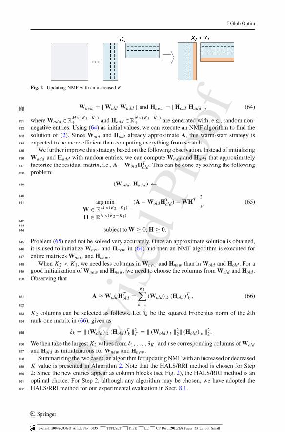
Fig. 2 Updating NMF with an increased K

Wnew = [Wold Wadd ] and Hnew = [Hold Hadd ], (64)829830

where Wadd ∈RM×(K2−K1)+ and Hadd ∈R

N×(K2−K1)+ are generated with, e.g., random non-831

negative entries. Using (64) as initial values, we can execute an NMF algorithm to find the832

solution of (2). Since Wold and Hold already approximate A, this warm-start strategy is833

expected to be more efficient than computing everything from scratch.834

We further improve this strategy based on the following observation. Instead of initializing835

Wadd and Hadd with random entries, we can compute Wadd and Hadd that approximately836

factorize the residual matrix, i.e., A−WoldHTold . This can be done by solving the following837

problem:838

(Wadd ,Hadd)←839

840

arg minW ∈ R

M×(K2−K1)

H ∈ RN×(K2−K1)

∥∥∥(A−WoldHT

old)−WHT∥∥∥

2

F(65)841

842843

subject to W ≥ 0,H ≥ 0.844

Problem (65) need not be solved very accurately. Once an approximate solution is obtained,845

it is used to initialize Wnew and Hnew in (64) and then an NMF algorithm is executed for846

entire matrices Wnew and Hnew .847

When K2 < K1, we need less columns in Wnew and Hnew than in Wold and Hold . For a848

good initialization of Wnew and Hnew, we need to choose the columns from Wold and Hold .849

Observing that850

A ≈WoldHTold =

K1∑

k=1

(Wold)·k (Hold)T·k , (66)851

852

K2 columns can be selected as follows. Let δk be the squared Frobenius norm of the kth853

rank-one matrix in (66), given as854

δk = ‖ (Wold)·k (Hold)T·k ‖2F = ‖ (Wold)·k ‖22‖ (Hold)·k ‖22.855

We then take the largest K2 values from δ1, . . . , δK1 and use corresponding columns of Wold856

and Hold as initializations for Wnew and Hnew .857

Summarizing the two cases, an algorithm for updating NMF with an increased or decreased858

K value is presented in Algorithm 2. Note that the HALS/RRI method is chosen for Step859

2: Since the new entries appear as column blocks (see Fig. 2), the HALS/RRI method is an860

optimal choice. For Step 2, although any algorithm may be chosen, we have adopted the861

HALS/RRI method for our experimental evaluation in Sect. 8.1.862

123


Rev

ised

Proo

f

J Glob Optim

Algorithm 2 Updating NMF with Increased or Decreased K Values

Input: A ∈ RM×N+ ,

(Wold ∈ R

M×K1+ ,Hold ∈ RN×K1+

)as a minimizer of (2), and K2.

Output:(

Wnew ∈ RM×K2+ ,Hnew ∈ R

N×K2+)

as a minimizer of (2).

1: if K2 > K1 then2: Approximately solve (65) with the HALS/RRI method to find (Wadd ,Hadd ).3: Let Wnew ← [Wold Wadd ] and Hnew ← [Hold Hadd ].4: end if5: if K2 < K1 then6: For k = 1, . . . , K1, let

δk = ‖ (Wold )·k ‖22‖ (Hold )·k ‖22.7: Let J be the indices corresponding to the K2 largest values of δ1, . . . , δK1 .8: Let Wnew and Hnew be the submatrices of Wold and Hold obtained from the columns indexed by J .9: end if10: Using Wnew and Hnew as initial values, execute an NMF algorithm to compute NMF of A.

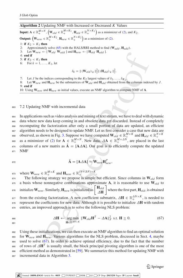
7.2 Updating NMF with incremental data863

In applications such as video analysis and mining of text stream, we have to deal with dynamic864

data where new data keep coming in and obsolete data get discarded. Instead of completely865

recomputing the factorization after only a small portion of data are updated, an efficient866

algorithm needs to be designed to update NMF. Let us first consider a case that new data are867

observed, as shown in Fig. 3. Suppose we have computed Wold ∈ RM×K+ and Hold ∈ R

N×K+868

as a minimizer of (2) for A ∈ RM×N+ . New data, ΔA ∈ R

M×ΔN+ , are placed in the last869

columns of a new matrix as A = [AΔA]. Our goal is to efficiently compute the updated870

NMF871

A = [AΔA] ≈WnewHTnew,872

where Wnew ∈ RM×K+ and Hnew ∈ R

(N+ΔN )×K+ .873

The following strategy we propose is simple but efficient. Since columns in Wold form874

a basis whose nonnegative combinations approximate A, it is reasonable to use Wold to875

initialize Wnew . Similarly, Hnew is initialized as

[Hold

ΔH

]where the first part, Hold , is obtained876

from the existing factorization. A new coefficient submatrix, ΔH ∈ RΔN×K+ , is needed to877

represent the coefficients for new data. Although it is possible to initialize ΔH with random878

entries, an improved approach is to solve the following NLS problem:879

ΔH← arg minH∈RΔN×K

‖WoldHT −ΔA‖2F s.t. H ≥ 0. (67)880

881

Using these initializations, we can then execute an NMF algorithm to find an optimal solution882

for Wnew and Hnew. Various algorithms for the NLS problem, discussed in Sect. 4, maybe883

used to solve (67). In order to achieve optimal efficiency, due to the fact that the number884

of rows of ΔHT is usually small, the block principal pivoting algorithm is one of the most885

efficient method as demonstrated in [59]. We summarize this method for updating NMF with886

incremental data in Algorithm 3.887

123


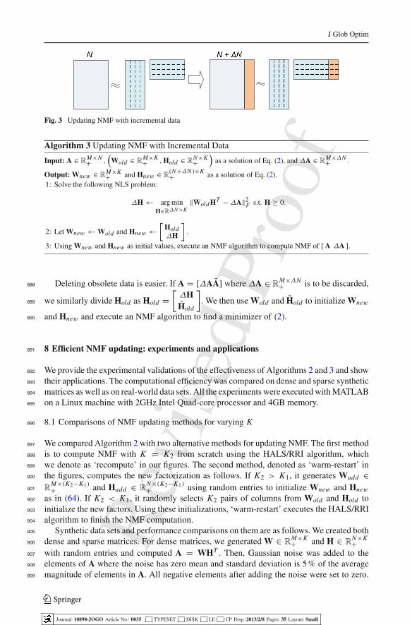
Rev

ised

Proo

f

J Glob Optim

Fig. 3 Updating NMF with incremental data

Algorithm 3 Updating NMF with Incremental Data

Input: A ∈ RM×N+ ,

(Wold ∈ R

M×K+ ,Hold ∈ RN×K+

)as a solution of Eq. (2), and ΔA ∈ R

M×ΔN+ .

Output: Wnew ∈ RM×K+ and Hnew ∈ R

(N+ΔN )×K+ as a solution of Eq. (2).

1: Solve the following NLS problem:

ΔH← arg minH∈RΔN×K

‖Wold HT −ΔA‖2F s.t. H ≥ 0.

2: Let Wnew ←Wold and Hnew ←[

HoldΔH

].

3: Using Wnew and Hnew as initial values, execute an NMF algorithm to compute NMF of [A ΔA ].

Deleting obsolete data is easier. If A = [ΔAA] where ΔA ∈ RM×ΔN+ is to be discarded,888

we similarly divide Hold as Hold =[ΔHHold

]. We then use Wold and Hold to initialize Wnew889

and Hnew and execute an NMF algorithm to find a minimizer of (2).890

8 Efficient NMF updating: experiments and applications891

We provide the experimental validations of the effectiveness of Algorithms 2 and 3 and show892

their applications. The computational efficiency was compared on dense and sparse synthetic893

matrices as well as on real-world data sets. All the experiments were executed with MATLAB894

on a Linux machine with 2GHz Intel Quad-core processor and 4GB memory.895

8.1 Comparisons of NMF updating methods for varying K896

We compared Algorithm 2 with two alternative methods for updating NMF. The first method897

is to compute NMF with K = K2 from scratch using the HALS/RRI algorithm, which898

we denote as ‘recompute’ in our figures. The second method, denoted as ‘warm-restart’ in899

the figures, computes the new factorization as follows. If K2 > K1, it generates Wadd ∈900

RM×(K2−K1)+ and Hadd ∈ R

N×(K2−K1)+ using random entries to initialize Wnew and Hnew901

as in (64). If K2 < K1, it randomly selects K2 pairs of columns from Wold and Hold to902

initialize the new factors. Using these initializations, ‘warm-restart’ executes the HALS/RRI903

algorithm to finish the NMF computation.904

Synthetic data sets and performance comparisons on them are as follows. We created both905

dense and sparse matrices. For dense matrices, we generated W ∈ RM×K+ and H ∈ R

N×K+906

with random entries and computed A = WHT . Then, Gaussian noise was added to the907

elements of A where the noise has zero mean and standard deviation is 5 % of the average908

magnitude of elements in A. All negative elements after adding the noise were set to zero.909

123


Rev

ised

Proo

f

J Glob Optim

We generated a 600×600 dense matrix with K = 80. For sparse matrices, we first generated910

W ∈ RM×K+ and H ∈ R

N×K+ with 90 % sparsity and computed A = WHT . We then used a911

soft-thresholding operation to obtain a sparse matrix A,1 and the resulting matrix had 88.2 %912

sparsity. We generated a synthetic sparse matrix of size 3, 000× 3, 000.2 In order to observe913

efficiency in updating, an NMF with K1 = 60 was first computed and stored. We then914

computed NMFs with K2 = 50, 65, and 80. The plots of relative error vs. execution time915

for all three methods are shown in Fig. 4. Our proposed method achieved faster convergence916

compared to ‘warm-restart’ and ‘recompute’, which sometimes required several times more917

computation to achieve the same accuracy as our method. The advantage of the proposed918

method can be seen in both dense and sparse cases.919

We have also used four real-world data sets for our comparisons. From the Topic Detection920

and Tracking 2 (TDT2) text corpus,3 we selected 40 topics to create a sparse term-document921

matrix of size 19, 009× 3, 087. From the 20 Newsgroups data set,4 a sparse term-document922

matrix of size 7, 845× 11, 269 was obtained after removing keywords and documents with923

frequency less than 20. The AT&T facial image database5 produced a dense matrix of size924

10, 304×400. The images in the CMU PIE database6 were resized to 64×64 pixels, and we925

formed a dense matrix of size 4, 096× 11, 554.7 We focused on the case when K increases,926

and the results are reported in Fig. 5. As with the synthetic data sets, our proposed method927

was shown to be the most efficient among the methods we tested.928

8.2 Applications of NMF updating for varying K929

Algorithm 2 can be used to determine the reduced dimension, K , from data. Our first example,930

shown in Fig. 6a, is determining a proper K value that represents the number of clusters.931

Using NMF as a clustering method [57,63], Brunet et al. [10] proposed to select the number932

of clusters by computing NMFs with multiple initializations for various K values and then933

evaluating the dispersion coefficients (See [10,52,57] for more details). We took the MNIST934

digit image database [65] and used 500 images with 28 × 28 pixels from each of the digits935

6, 7, 8, and 9. The resulting data matrix was of size 784 × 2, 000. We computed NMFs for936

K = 3, 4, 5, and 6 with 50 different initializations for each K . The top of Fig. 6a shows937

that K = 4 can be correctly determined from the point where the dispersion coefficient938

starts to drop. The bottom of Fig. 6a shows the box-plot of the total execution time needed939

by Algorithm 2, ‘recompute’, and ‘warm-restart’. We applied the same stopping criterion in940

(62) for all three methods.941

Further applications of Algorithm 2 are shown in Fig. 6b, c. Figure 6b demonstrates a942

process of probing the approximation errors of NMF with various K values. With K =943

20, 40, 60 and 80, we generated 600×600 synthetic dense matrices as described in Sect. 8.1.944

Then, we computed NMFs with Algorithm 2 for K values ranging from 10 to 160 with a step945

size 5. The relative objective function values with respect to K are shown in Fig. 6b. In each946

of the cases where K = 20, 40, 60, and 80, we were able to determine the correct K value947

by choosing a point where the relative error stopped decreasing significantly.948

1 For each element ai j , we used ai j ← max(ai j − 2, 0).2 We created a larger matrix for the sparse case to clearly illustrate the relative efficiency.3 http://projects.ldc.upenn.edu/TDT2/.4 http://people.csail.mit.edu/jrennie/20Newsgroups/.5 http://www.cl.cam.ac.uk/research/dtg/attarchive/facedatabase.html.6 http://www.ri.cmu.edu/projects/project_418.html.7 http://www.zjucadcg.cn/dengcai/Data/FaceData.html.

123


http://projects.ldc.upenn.edu/TDT2/

http://people.csail.mit.edu/jrennie/20Newsgroups/

http://www.cl.cam.ac.uk/research/dtg/attarchive/facedatabase.html

http://www.ri.cmu.edu/projects/project_418.html

http://www.zjucadcg.cn/dengcai/Data/FaceData.html

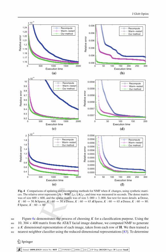
Rev

ised

Proo

f

J Glob Optim

0 500 1000 1500 2000

1.16

1.17

1.18

1.19

1.2

1.21

1.22

1.23

1.24

x 10−3

Execution time

Rel

ativ

e er

ror

RecomputeWarm−restartOur method

0 50 100 150 200 250 3000.036

0.036

0.036

0.036

0.036

0.036

Execution time

Rel

ativ

e er

ror


0 500 1000 1500 20009.2

9.3

9.4

9.5

9.6

9.7

9.8

9.9

10x 10

−4

Execution time

Rel

ativ

e er

ror


0 50 100 150 200

0.0357

0.0357

0.0358

0.0358

0.0358

0.0358

Execution time

Rel

ativ

e er

ror


0 500 1000 1500 2000

0.4

0.6

0.8

1

1.2

1.4

1.6

1.8

2x 10

−3

Execution time

Rel

ativ

e er

ror


0 50 100 150 200 250 300

0.0355

0.0355

0.0355

0.0355

0.0355

0.0355

0.0356

0.0356

0.0356

0.0356

0.0356

Execution time

Rel

ativ

e er

ror


(a)

(c)

(e) (f)

(d)

(b)

Fig. 4 Comparisons of updating and recomputing methods for NMF when K changes, using synthetic matri-ces. The relative error represents ‖A−WHT ‖F/‖A‖F , and time was measured in seconds. The dense matrixwas of size 600× 600, and the sparse matrix was of size 3, 000× 3, 000. See text for more details. a Dense,K : 60→ 50. b Sparse, K : 60→ 50. c Dense, K : 60→ 65. d Sparse, K : 60→ 65. e Dense, K : 60→ 80.f Sparse, K : 60→ 80

Figure 6c demonstrates the process of choosing K for a classification purpose. Using the949

10, 304× 400 matrix from the AT&T facial image database, we computed NMF to generate950

a K dimensional representation of each image, taken from each row of H. We then trained a951

nearest neighbor classifier using the reduced-dimensional representations [83]. To determine952

123


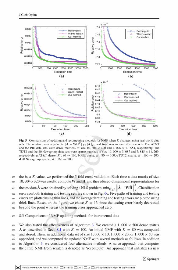
Rev

ised

Proo

f

J Glob Optim

0 500 1000 1500 2000 2500 3000 3500

0.0168

0.0169

0.0169

0.017

0.017

0.017

Execution time

Rel

ativ

e er

ror


0 1000 2000 3000 4000 5000 6000

7.25

7.3

7.35

7.4

7.45

7.5x 10

−3

Execution time

Rel

ativ

e er

ror


0 50 100 150 200 250

0.024

0.024

0.0241

0.0241

0.0242

0.0242

0.0243

Execution time

Rel

ativ

e er

ror


0 200 400 600 800 1000

6.38

6.39

6.4

6.41

6.42

6.43

6.44

6.45

6.46

6.47

6.48

x 10−3

Execution time

Rel

ativ

e er

ror Recompute

Warm−restartOur method

(a)

(c)

(b)

(d)

Fig. 5 Comparisons of updating and recomputing methods for NMF when K changes, using real-world datasets. The relative error represents ‖A − WHT ‖F/‖A‖F , and time was measured in seconds. The AT&Tand the PIE data sets were dense matrices of size 10, 304 × 400 and 4, 096 × 11, 554, respectively. TheTDT2 and the 20 Newsgroup data sets were sparse matrices of size 19, 009 × 3, 087 and 7, 845 × 11, 269,respectively. a AT&T, dense, K : 80→ 100, b PIE, dense, K : 80→ 100, c TDT2, sparse, K : 160→ 200,d 20 Newsgroup, sparse, K : 160→ 200

the best K value, we performed the 5-fold cross validation: Each time a data matrix of size953

10, 304×320 was used to compute W and H, and the reduced-dimensional representations for954

the test data A were obtained by solving a NLS problem, minH≥0

∥∥∥A−WH

∥∥∥

2

F. Classification955

errors on both training and testing sets are shown in Fig. 6c. Five paths of training and testing956

errors are plotted using thin lines, and the averaged training and testing errors are plotted using957

thick lines. Based on the figure, we chose K = 13 since the testing error barely decreased958

beyond the point whereas the training error approached zero.959

8.3 Comparisons of NMF updating methods for incremental data960

We also tested the effectiveness of Algorithm 3. We created a 1, 000 × 500 dense matrix961

A as described in Sect. 8.1 with K = 100. An initial NMF with K = 80 was computed962

and stored. Then, an additional data set of size 1, 000× 10, 1, 000× 20, or 1, 000× 50 was963

appended, and we computed the updated NMF with several methods as follows. In addition964

to Algorithm 3, we considered four alternative methods. A naive approach that computes965

the entire NMF from scratch is denoted as ‘recompute’. An approach that initializes a new966

123


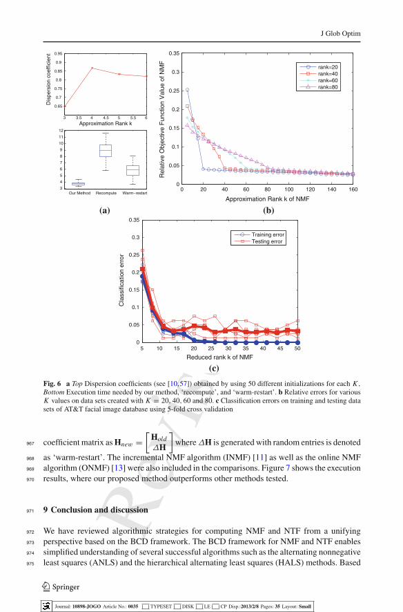
Rev

ised

Proo

f

J Glob Optim

3 3.5 4 4.5 5 5.5 6

0.65

0.7

0.75

0.8

0.85

0.9

0.95

Approximation Rank k

Dis

pers

ion

coef

ficie

nt

Our Method Recompute Warm−restart3

4

5

6

7

8

9

10

11

12

0 20 40 60 80 100 120 140 1600

0.05

0.1

0.15

0.2

0.25

0.3

0.35

Approximation Rank k of NMF

Rel

ativ

e O

bjec

tive

Fun

ctio

n V

alue

of N

MF

rank=20rank=40rank=60rank=80

5 10 15 20 25 30 35 40 45 500

0.05

0.1

0.15

0.2

0.25

0.3

0.35

Reduced rank k of NMF

Cla

ssifi

catio

n er

ror

Training errorTesting error

(a) (b)

(c)

Fig. 6 a Top Dispersion coefficients (see [10,57]) obtained by using 50 different initializations for each K ,Bottom Execution time needed by our method, ‘recompute’, and ‘warm-restart’. b Relative errors for variousK values on data sets created with K = 20, 40, 60 and 80. c Classification errors on training and testing datasets of AT&T facial image database using 5-fold cross validation

coefficient matrix as Hnew =[

Hold

ΔH

]whereΔH is generated with random entries is denoted967

as ‘warm-restart’. The incremental NMF algorithm (INMF) [11] as well as the online NMF968

algorithm (ONMF) [13] were also included in the comparisons. Figure 7 shows the execution969

results, where our proposed method outperforms other methods tested.970

9 Conclusion and discussion971

We have reviewed algorithmic strategies for computing NMF and NTF from a unifying972

perspective based on the BCD framework. The BCD framework for NMF and NTF enables973

simplified understanding of several successful algorithms such as the alternating nonnegative974

least squares (ANLS) and the hierarchical alternating least squares (HALS) methods. Based975

123


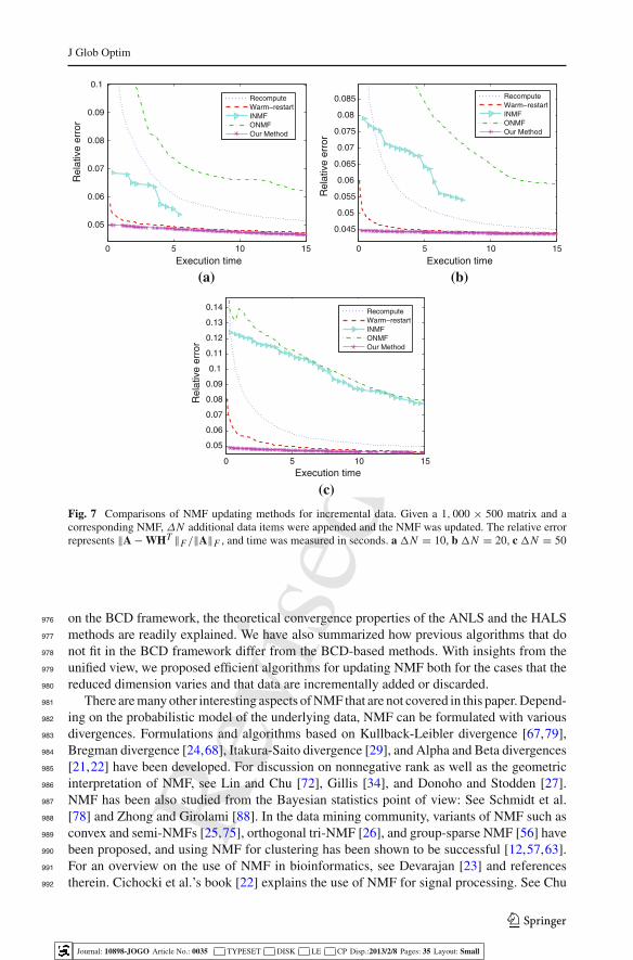
Rev

ised

Proo

f

J Glob Optim

0 5 10 15

0.05

0.06

0.07

0.08

0.09

0.1

Execution time

Rel

ativ

e er

ror

RecomputeWarm−restartINMFONMFOur Method

(a)

0 5 10 15

0.045

0.05

0.055

0.06

0.065

0.07

0.075

0.08

0.085

Execution time

Rel

ativ

e er

ror


(b)

0 5 10 15

0.05

0.06

0.07

0.08

0.09

0.1

0.11

0.12

0.13

0.14

Execution time

Rel

ativ

e er

ror


(c)

Fig. 7 Comparisons of NMF updating methods for incremental data. Given a 1, 000 × 500 matrix and acorresponding NMF, ΔN additional data items were appended and the NMF was updated. The relative errorrepresents ‖A−WHT ‖F/‖A‖F , and time was measured in seconds. a N = 10, b N = 20, c N = 50

on the BCD framework, the theoretical convergence properties of the ANLS and the HALS976

methods are readily explained. We have also summarized how previous algorithms that do977

not fit in the BCD framework differ from the BCD-based methods. With insights from the978

unified view, we proposed efficient algorithms for updating NMF both for the cases that the979

reduced dimension varies and that data are incrementally added or discarded.980

There are many other interesting aspects of NMF that are not covered in this paper. Depend-981

ing on the probabilistic model of the underlying data, NMF can be formulated with various982

divergences. Formulations and algorithms based on Kullback-Leibler divergence [67,79],983

Bregman divergence [24,68], Itakura-Saito divergence [29], and Alpha and Beta divergences984

[21,22] have been developed. For discussion on nonnegative rank as well as the geometric985

interpretation of NMF, see Lin and Chu [72], Gillis [34], and Donoho and Stodden [27].986

NMF has been also studied from the Bayesian statistics point of view: See Schmidt et al.987

[78] and Zhong and Girolami [88]. In the data mining community, variants of NMF such as988

convex and semi-NMFs [25,75], orthogonal tri-NMF [26], and group-sparse NMF [56] have989

been proposed, and using NMF for clustering has been shown to be successful [12,57,63].990

For an overview on the use of NMF in bioinformatics, see Devarajan [23] and references991

therein. Cichocki et al.’s book [22] explains the use of NMF for signal processing. See Chu992

123


Rev

ised

Proo

f

J Glob Optim

and Plemmons [17], Berry et al. [4], and Cichocki et al. [22] for earlier surveys on NMF. See993

also Ph.D. dissertations on NMF algorithms and applications [34,44,55].994

995

Open Access This article is distributed under the terms of the Creative Commons Attribution License which996

permits any use, distribution, and reproduction in any medium, provided the original author(s) and the source997

are credited.998

References999

1. Acar, E., Yener, B.: Unsupervised multiway data analysis: a literature survey. IEEE Trans. Knowl. Data1000

Eng. 21(1), 6–20 (2009)1001

2. Bellavia, S., Macconi, M., Morini, B.: An interior point newton-like method for non-negative least-squares1002

problems with degenerate solution. Numer. Linear Algebra Appl. 13(10), 825–846 (2006)1003

3. Berman, A., Plemmons, R.J.: Nonnegative matrices in the mathematical sciences. Society for Industrial1004

and Applied Mathematics, Philadelphia (1994)1005

4. Berry, M., Browne, M., Langville, A., Pauca, V., Plemmons, R.: Algorithms and applications for approx-1006

imate nonnegative matrix factorization. Comput. Stat. Data Anal. 52(1), 155–173 (2007)1007

5. Bertsekas, D.P.: Nonlinear programming. Athena Scientific (1999)1008

6. Biggs, M., Ghodsi, A., Vavasis, S.: Nonnegative matrix factorization via rank-one downdate. In: Proceed-1009

ings of the 25th International Conference on, Machine Learning, pp. 64–71 (2008)1010

7. Birgin, E., Martínez, J., Raydan, M.: Nonmonotone spectral projected gradient methods on convex sets.1011

SIAM J. Optim. 10(4), 1196–1211 (2000)1012

8. Björck, Å.: Numerical Methods for Least Squares Problems. Society for Industrial and Applied Mathe-1013

matics, Philadelphia (1996)1014

9. Bro, R., De Jong, S.: A fast non-negativity-constrained least squares algorithm. J. Chemom. 11, 393–4011015

(1997)1016

10. Brunet, J., Tamayo, P., Golub, T., Mesirov, J.: Metagenes and molecular pattern discovery using matrix1017

factorization. Proc. Natal. Acad. Sci. 101(12), 4164–4169 (2004)1018

11. Bucak, S., Gunsel, B.: Video content representation by incremental non-negative matrix factoriza-1019

tion. In: Proceedings of the 2007 IEEE International Conference on Image Processing (ICIP), vol. 2,1020

pp. II-113–II-116 (2007)1021

12. Cai, D., He, X., Han, J., Huang, T.: Graph regularized nonnegative matrix factorization for data represen-1022

tation. IEEE Trans. Pattern Anal. Mach. Intell. 33(8), 1548–1560 (2011)1023

13. Cao, B., Shen, D., Sun, J.T., Wang, X., Yang, Q., Chen, Z.: Detect and track latent factors with online1024

nonnegative matrix factorization. In: Proceedings of the 20th International Joint Conference on Artifical,1025

Intelligence, pp. 2689–2694 (2007)1026

14. Carroll, J.D., Chang, J.J.: Analysis of individual differences in multidimensional scaling via an n-way1027

generalization of ”eckart-young” decomposition. Psychometrika 35(3), 283–319 (1970)1028

15. Chen, D., Plemmons, R.J.: Nonnegativity constraints in numerical analysis. In: Proceedings of the1029

Symposium on the Birth of Numerical Analysis, Leuven Belgium, pp. 109–140 (2009)1030

16. Chen, S.S., Donoho, D.L., Saunders, M.A.: Atomic decomposition by basis pursuit. SIAM Rev. 43(1),1031

129–159 (2001)1032

17. Chu, M., Plemmons, R.: Nonnegative matrix factorization and applications. IMAGE: Bull. Int. Linear1033

Algebra Soc. 34, 2–7 (2005)1034

18. Chu, M.T., Lin, M.M.: Low-dimensional polytope approximation and its applications to nonnegative1035

matrix factorization. SIAM J. Sci. Comput. 30(3), 1131–1155 (2008)1036

19. Cichocki, A., Phan, A.H.: Fast local algorithms for large scale nonnegative matrix and tensor factoriza-1037

tions. IEICE Trans. Fundam. Electron. Commun. Comput. Sci. E92-A(3), 708–721 (2009)1038

20. Cichocki, A., Zdunek, R., Amari, S.I.: Hierarchical ALS algorithms for nonnegative matrix and 3d tensor1039

factorization. In: Lecture Notes in Computer Science, vol. 4666, pp. 169–176. Springer (2007)1040

21. Cichocki, A., Zdunek, R., Choi, S., Plemmons, R., Amari, S.-I.: Nonnegative tensor factorization using1041

alpha and beta divergencies. In: Proceedings of the 32nd International Conference on Acoustics, Speech,1042

and Signal Processing (ICASSP), Honolulu, April 2007, vol. 3, pp. III-1393–III-1396 (2007)1043

22. Cichocki, A., Zdunek, R., Phan, A.H., Amari, S.I.: Nonnegative Matrix and Tensor Factorizations: Appli-1044

cations to Exploratory Multi-Way Data Analysis and Blind Source Separation. Wiley, West Sussex (2009)1045

23. Devarajan, K.: Nonnegative matrix factorization: an analytical and interpretive tool in computational1046

biology. PLoS Comput. Biol. 4(7), e1000,029 (2008)1047

123


Rev

ised

Proo

f

J Glob Optim

24. Dhillon, I., Sra, S.: Generalized nonnegative matrix approximations with bregman divergences. In:1048

Advances in Neural Information Processing Systems 18, pp. 283–290. MIT Press (2006)1049

25. Ding, C., Li, T., Jordan, M.: Convex and semi-nonnegative matrix factorizations. IEEE Trans. Pattern1050

Anal. Mach. Intell. 32(1), 45–559 (2010)1051

26. Ding, C., Li, T., Peng, W., Park, H.: Orthogonal nonnegative matrix tri-factorizations for clustering. In:1052

Proceedings of the 12th ACM SIGKDD International Conference on Knowledge Discovery and Data1053

Mining, pp. 126–135 (2006)1054

27. Donoho, D., Stodden, V.: When does non-negative matrix factorization give a correct decomposition into1055

parts? In: Advances in Neural Information Processing Systems 16. MIT Press (2004)1056

28. Drake, B., Kim, J., Mallick, M., Park, H.: Supervised Raman spectra estimation based on nonnegative1057

rank deficient least squares. In: Proceedings of the 13th International Conference on Information Fusion,1058

Edinburgh, UK (2010)1059

29. Févotte, C., Bertin, N., Durrieu, J.: Nonnegative matrix factorization with the Itakura-Saito divergence:1060

With application to music analysis. Neural Comput. 21(3), 793–830 (2009)1061

30. Figueiredo, M.A.T., Nowak, R.D., Wright, S.J.: Gradient projection for sparse reconstruction: application1062

to compressed sensing and other inverse problems. IEEE J. Sel. Top. Signal Process. 1(4), 586–597 (2007)1063

31. Franc, V., Hlavac, V., Navara, M.: Sequential coordinate-wise algorithm for the non-negative least squares1064

problem. In: Proceedings of the 11th International Conference on Computer Analysis of Images and1065

Patterns, pp. 407–414 (2005)1066

32. Friedlander, M.P., Hatz, K.: Computing nonnegative tensor factorizations. Comput. Optim. Appl. 23(4),1067

631–647 (2008)1068

33. Frigyesi, A., Höglund, M.: Non-negative matrix factorization for the analysis of complex gene expression1069

data: identification of clinically relevant tumor subtypes. Cancer Inform. 6, 275–292 (2008)1070

34. Gillis, N.: Nonnegative matrix factorization complexity, algorithms and applications. Ph.D. thesis,1071

Université catholique de Louvain (2011)1072

35. Gillis, N., Glineur, F.: Nonnegative factorization and the maximum edge biclique problem. CORE1073

Discussion Paper 2008/64, Universite catholique de Louvain (2008)1074

36. Gillis, N., Glineur, F.: Using underapproximations for sparse nonnegative matrix factorization. Pattern1075

Recognit. 43(4), 1676–1687 (2010)1076

37. Gillis, N., Glineur, F.: Accelerated multiplicative updates and hierarchical als algorithms for nonnegative1077

matrix factorization. Neural Comput. 24(4), 1085–1105 (2012)1078

38. Gillis, N., Glineur, F.: A multilevel approach for nonnegative matrix factorization. J. Comput. Appl. Math.1079

236, 1708–1723 (2012)1080

39. Golub, G., Van Loan, C.: Matrix Computations. Johns Hopkins University Press, Baltimore (1996)1081

40. Gonzalez, E.F., Zhang, Y.: Accelerating the lee-seung algorithm for non-negative matrix factorization.1082

Department of Computational and Applied Mathematics, Rice University, Technical report (2005)1083

41. Grippo, L., Sciandrone, M.: On the convergence of the block nonlinear gauss-seidel method under convex1084

constraints. Oper. Res. Lett. 26(3), 127–136 (2000)1085

42. Han, L., Neumann, M., Prasad, U.: Alternating projected Barzilai-Borwein methods for nonnegative1086

matrix factorization. Electron. Trans. Numer. Anal. 36, 54–82 (2009)1087

43. Harshman, R.A.: Foundations of the parafac procedure: models and conditions for an ”explanatory”1088

multi-modal factor analysis. In: UCLA Working Papers in Phonetics, vol. 16, pp. 1–84 (1970)1089

44. Ho, N.D.: Nonnegative matrix factorization algorithms and applications. Ph.D. thesis, Univ. Catholique1090

de Louvain (2008)1091

45. Horn, R.A., Johnson, C.R.: Matrix Analysis. Cambridge University Press, Cambridge (1990)1092

46. Horst, R., Pardalos, P., Van Thoai, N.: Introduction to Global Optimization. Kluwer, Berlin (2000)1093

47. Hoyer, P.O.: Non-negative matrix factorization with sparseness constraints. J. Mach. Learn. Res. 5,1094

1457–1469 (2004)1095

48. Hsieh, C.J., Dhillon, I.S.: Fast coordinate descent methods with variable selection for non-negative1096

matrix factorization. In: Proceedings of the 17th ACM SIGKDD International Conference on Knowledge1097

Discovery and Data Mining, pp. 1064–1072 (2011)1098

49. Hutchins, L., Murphy, S., Singh, P., Graber, J.: Position-dependent motif characterization using non-1099

negative matrix factorization. Bioinformatics 24(23), 2684–2690 (2008)1100

50. Júdice, J.J., Pires, F.M.: A block principal pivoting algorithm for large-scale strictly monotone linear1101

complementarity problems. Comput. Oper. Res. 21(5), 587–596 (1994)1102

51. Kim, D., Sra, S., Dhillon, I.S.: Fast Newton-type methods for the least squares nonnegative matrix approxi-1103

mation problem. In: Proceedings of the 2007 SIAM International Conference on Data Mining, pp. 343–3541104

(2007)1105

52. Kim, H., Park, H.: Sparse non-negative matrix factorizations via alternating non-negativity-constrained1106

least squares for microarray data analysis. Bioinformatics 23(12), 1495–1502 (2007)1107

123


Rev

ised

Proo

f

J Glob Optim

53. Kim, H., Park, H.: Nonnegative matrix factorization based on alternating nonnegativity constrained least1108

squares and active set method. SIAM J. Matrix Anal. Appl. 30(2), 713–730 (2008)1109

54. Kim, H., Park, H., Eldén, L.: Non-negative tensor factorization based on alternating large-scale non-1110

negativity-constrained least squares. In: Proceedings of IEEE 7th International Conference on Bioinfor-1111

matics and, Bioengineering (BIBE07), vol. 2, pp. 1147–1151 (2007)1112

55. Kim, J.: Nonnegative Matrix and Tensor Factorizations, Least Squares Problems, and Applications. Ph.D.1113

Thesis, Georgia Institute of Technology (2011)1114

56. Kim, J., Monteiro, R.D., Park, H.: Group Sparsity in Nonnegative Matrix Factorization. In: Proceedings1115

of the 2012 SIAM International Conference on Data Mining, pp 851–862 (2012)1116

57. Kim, J., Park, H.: Sparse nonnegative matrix factorization for clustering. Technical report, Georgia1117

Institute of Technology GT-CSE-08-01 (2008)1118

58. Kim, J., Park, H.: Toward faster nonnegative matrix factorization: a new algorithm and comparisons. In:1119

Proceedings of the 8th IEEE International Conference on Data Mining (ICDM), pp. 353–362 (2008)1120

59. Kim, J., Park, H.: Fast nonnegative matrix factorization: an active-set-like method and comparisons.1121

SIAM J. Sci. Comput. 33(6), 3261–3281 (2011)1122

60. Kim, J., Park, H.: Fast nonnegative tensor factorization with an active-set-like method. In: High-1123

Performance Scientific Computing: Algorithms and Applications, pp. 311–326. Springer (2012)1124

61. Kolda, T.G., Bader, B.W.: Tensor decompositions and applications. SIAM Rev. 51(3), 455–500 (2009)1125

62. Korattikara, A., Boyles, L., Welling, M., Kim, J., Park, H.: Statistical optimization of non-negative matrix1126

factorization. In: Proceedings of the 14th International Conference on Artificial Intelligence and Statistics1127

(AISTATS), JMLR: W&CP, vol. 15, pp. 128–136 (2011)1128

63. Kuang, D., Ding, C., Park, H.: Symmetric nonnegative matrix factorization for graph clustering. In:1129

Proceedings of 2012 SIAM International Conference on Data Mining, pp. 106–117 (2012)1130

64. Lawson, C.L., Hanson, R.J.: Solving Least Squares Problems. Prentice Hall, New Jersey (1974)1131

65. LeCun, Y., Bottou, L., Bengio, Y., Haffner, P.: Gradient-based learning applied to document recognition.1132

Proc. IEEE 86(11), 2278–2324 (1998)1133

66. Lee, D.D., Seung, H.S.: Learning the parts of objects by non-negative matrix factorization. Nature1134

401(6755), 788–791 (1999)1135

67. Lee, D.D., Seung, H.S.: Algorithms for non-negative matrix factorization. In: Advances in Neural Infor-1136

mation Processing Systems 13, pp. 556–562. MIT Press (2001)1137

68. Li, L., Lebanon, G., Park, H.: Fast bregman divergence nmf using taylor expansion and coordinate descent.1138

In: Proceedings of the 18th ACM SIGKDD international conference on Knowledge discovery and data1139

mining, pp. 307–315 (2012)1140

69. Li, S.Z., Hou, X., Zhang, H., Cheng, Q.: Learning spatially localized, parts-based representation.1141

In: Proceedings of the 2001 IEEE Computer Society Conference on Computer Vision and, Pattern Recog-1142

nition, vol. 1, pp. I-207–I-212 (2001)1143

70. Lin, C.: On the convergence of multiplicative update algorithms for nonnegative matrix factorization.1144

IEEE Trans. Neural Netw. 18(6), 1589–1596 (2007)1145

71. Lin, C.J.: Projected gradient methods for nonnegative matrix factorization. Neural Comput. 19(10),1146

2756–2779 (2007)1147

72. Lin, M.M., Chu, M.T.: On the nonnegative rank of euclidean distance matrices. Linear Algebra Appl.1148

433(3), 681–689 (2010)1149

73. Merritt, M., Zhang, Y.: Interior-point gradient method for large-scale totally nonnegative least squares1150

problems. J. optim. Theory Appl. 126(1), 191–202 (2005)1151

74. Paatero, P., Tapper, U.: Positive matrix factorization: a non-negative factor model with optimal utilization1152

of error estimates of data values. Environmetrics 5(1), 111–126 (1994)1153

75. Park, H., Kim, H.: One-sided non-negative matrix factorization and non-negative centroid dimension1154

reduction for text classification. In: Proceedings of the 2006 Text Mining Workshop in the Tenth SIAM1155

International Conference on Data Mining (2006)1156

76. Pauca, V.P., Piper, J., Plemmons, R.J.: Nonnegative matrix factorization for spectral data analysis. Linear1157

Algebra Appl. 416(1), 29–47 (2006)1158

77. Pauca, V.P., Shahnaz, F., Berry, M.W., Plemmons, R.J.: Text mining using non-negative matrix factoriza-1159

tions. In: Proceedings of the 2004 SIAM International Conference on Data Mining, pp. 452–456 (2004)1160

78. Schmidt, M.N., Winther, O., Hansen, L.K.: Bayesian non-negative matrix factorization. In: Proceedings1161

of the 2009 International Conference on Independent Component Analysis and Signal Separation, Lecture1162

Notes in Computer Science (LNCS), vol. 5441, pp. 540–547. Springer (2009)1163

79. Sra, S.: Block-iterative algorithms for non-negative matrix approximation. In: Proceedings of the 8th1164

IEEE International Conference on Data Mining, pp. 1037–1042 (2008)1165

80. Tibshirani, R.: Regression shrinkage and selection via the lasso. J. R. Stat. Soc. Ser. B (Methodological)1166

58(1), 267–288 (1996)1167

123


Rev

ised

Proo

f

J Glob Optim

81. Van Benthem, M.H., Keenan, M.R.: Fast algorithm for the solution of large-scale non-negativity-1168

constrained least squares problems. J. Chemom. 18, 441–450 (2004)1169

82. Vavasis, S.A.: On the complexity of nonnegative matrix factorization. SIAM J. Optim. 20(3), 1364–13771170

(2009)1171

83. Weinberger, K., Saul, L.: Distance metric learning for large margin nearest neighbor classification.1172

J. Mach. Learn. Res. 10, 207–244 (2009)1173

84. Welling, M., Weber, M.: Positive tensor factorization. Pattern Recogn. Lett. 22(12), 1255–1261 (2001)1174

85. Xu, W., Liu, X., Gong, Y.: Document clustering based on non-negative matrix factorization. In: Pro-1175

ceedings of the 26th Annual International ACM SIGIR Conference on Research and Development in1176

Informaion Retrieval, pp. 267–273 (2003)1177

86. Zdunek, R., Cichocki, A.: Non-negative matrix factorization with quasi-newton optimization. In: Proceed-1178

ings of the Eighth International Conference on Artificial Intelligence and, Soft Computing, pp. 870–8791179

(2006)1180

87. Zdunek, R., Cichocki, A.: Fast nonnegative matrix factorization algorithms using projected gradient1181

approaches for large-scale problems. Comput. Intell. Neurosci. 2008, 939567 (2008)1182

88. Zhong, M., Girolami, M.: Reversible jump MCMC for non-negative matrix factorization. In: Proceed-1183

ings of the Twelfth International Conference on Artificial Intelligence and Statistics (AISTATS), JMLR:1184

W&CP, vol. 5, pp. 663–670 (2009)1185

123


algorithms for nonnegative matrix and tensor ...hpark/papers/jgo.pdf · proof j glob optim doi...

Documents