align, then memorise: the dynamics of learning with

Align, then memorise:the dynamics of learning with feedback alignment

Maria Refinetti * 1 2 Stephane d’Ascoli * 1 3 Ruben Ohana 1 4 Sebastian Goldt 5

AbstractDirect Feedback Alignment (DFA) is emergingas an efficient and biologically plausible alterna-tive to backpropagation for training deep neuralnetworks. Despite relying on random feedbackweights for the backward pass, DFA successfullytrains state-of-the-art models such as Transform-ers. On the other hand, it notoriously fails to trainconvolutional networks. An understanding of theinner workings of DFA to explain these diverg-ing results remains elusive. Here, we proposea theory of feedback alignment algorithms. Wefirst show that learning in shallow networks pro-ceeds in two steps: an alignment phase, where themodel adapts its weights to align the approximategradient with the true gradient of the loss function,is followed by a memorisation phase, where themodel focuses on fitting the data. This two-stepprocess has a degeneracy breaking effect: out ofall the low-loss solutions in the landscape, a net-work trained with DFA naturally converges to thesolution which maximises gradient alignment. Wealso identify a key quantity underlying alignmentin deep linear networks: the conditioning of thealignment matrices. The latter enables a detailedunderstanding of the impact of data structure onalignment, and suggests a simple explanation forthe well-known failure of DFA to train convolu-tional neural networks. Numerical experimentson MNIST and CIFAR10 clearly demonstrate de-generacy breaking in deep non-linear networksand show that the align-then-memorize processoccurs sequentially from the bottom layers of thenetwork to the top.

*Equal contribution 1Department of Physics, Ecole NormaleSuperieure, Paris, France 2IdePHICS laboratory, EPFL 3FacebookAI Research, Paris, France 4LightOn, Paris, France 5InternationalSchool of Advanced Studies (SISSA), Trieste, Italy. Correspon-dence to: Sebastian Goldt <[email protected]>.

Proceedings of the 38 th International Conference on MachineLearning, PMLR 139, 2021. Copyright 2021 by the author(s).

IntroductionTraining a deep neural network on a supervised learningtask requires solving the credit assignment problem: howshould weights deep in the network be changed, given onlythe output of the network and the target label of the input?Today, almost all networks from computer vision to naturallanguage processing solve this problem using variants ofthe back-propagation algorithm (BP) popularised severaldecades ago by Rumelhart et al. (1986). For concreteness,we illustrate BP using a fully-connected deep network ofdepthLwith weightsWl in the lth layer. Given an input x ≡h0, the output y of the network is computed sequentially asy = fy(aL), with al = Wlhl−1 and hl = g(al), where g isa pointwise non-linearity. For regression, the loss functionJ is the mean-square error and fy is the identity. Given theerror e ≡ ∂J/∂aL = y − y of the network on an input x, theupdate of the last layer of weights reads

δWL = −ηeh>L−1 (1)

for a learning rate η. The updates of the layers below aregiven by δWl = −ηδalhTl−1, with factors δal defined se-quentially as

δaBPl = ∂J/∂al =

(WTl+1δal+1

)� g′ (al) , (2)

with � denoting the Hadamard product. BP thus solves thecredit assignment problem for deeper layers of the networkby using the transpose of the network’s weight matrices totransmit the error signal across the network from one layerto the next, see Fig. 1.

Despite its popularity and practical success, BP suffers fromseveral limitations. First, it relies on symmetric weightsfor the forward and backward pass, which makes it a bio-logically implausible learning algorithm (Grossberg, 1987;Crick, 1989). Second, BP updates layers sequentially duringthe backward pass, preventing an efficient parallelisation oftraining, which becomes ever more important as state-of-the-art networks grow larger and deeper.

In light of these shortcomings, algorithms which only ap-proximate the gradient of the loss are attracting increasinginterest. Lillicrap et al. (2016) demonstrated that neuralnetworks can be trained successfully even if the transpose

The Dynamics of Learning with Feedback Alignment

x y

δW1 δW3δW2

W1 W2 W3W4

eW⊤2 W⊤3 W⊤4

δW1 δW3δW2 eF1 F2 F3

δW1 δW3δW2F1 F2 F3

e

BP(Rumelhart et al. ’86)

FA(Lillicrap et al. ’14)

DFA(Nøkland ’16)

Figure 1. Three approaches to the credit assignment problemin deep neural networks. In back-propagation (BP), the weightupdates δWl are computed sequentially by transmitting the error efrom layer to layer using the transpose of the network’s weightsW>l . In feedback alignment (FA) (Lillicrap et al., 2016), W>lare replaced by fixed random feedback matrices Fl. In directfeedback alignment (DFA) (Nøkland, 2016), the error is directlyinjected to each layer using random feedback matrices Fl, enablingparallelized training.

of the network weights W>l are replaced by random feed-back connections Fl in the backward pass, an algorithm theycalled “feedback alignment” (FA):

δaFAl = (Flδal+1)� g′ (al) . (3)

In this way, they dispense with the need of biologically unre-alistic symmetric forward and backward weights (Grossberg,1987; Crick, 1989). The “direct feedback alignment” (DFA)algorithm of Nøkland (2016) takes this idea one step furtherby propagating the error directly from the output layer toeach hidden layer of the network through random feedbackconnections Fl:

δaDFAl = (Fle)� g′ (al) . (4)

DFA thus allows updating different layers in parallel. Fig. 1shows the information flow of all three algorithms.

While it was initially unclear whether DFA could scaleto challenging datasets and complex architectures (Gilmeret al., 2017; Bartunov et al., 2018), recently Launay et al.(2020) obtained performances comparable to fine-tuned BPwhen using DFA to train a number of state-of-the-art archi-tectures on problems ranging from neural view synthesisto natural language processing. Yet, feedback alignmentnotoriously fails to train convolutional networks (Bartunov

et al., 2018; Moskovitz et al., 2018; Launay et al., 2019;Han & Yoo, 2019). These varied results underline the needfor a theoretical understanding of how and when feedbackalignment works.

Related Work Lillicrap et al. (2016) gave a first theoreti-cal characterisation of feedback alignment by arguing thatfor two-layer linear networks, FA works because the trans-pose of the second layer of weights W2 tends to align withthe random feedback matrix F1 during training. This weightalignment (WA) leads the weight updates of FA to alignwith those of BP, leading to gradient alignment (GA) andthus to successful learning. Frenkel et al. (2019) extendedthis analysis to the deep linear case for a variant of DFAcalled “Direct Random Target Projection” (DRTP), underthe restrictive assumption of training on a single data point.Nøkland (2016) also introduced a layerwise alignment cri-terion to describe DFA in the deep nonlinear setup, underthe assumption of constant update directions for each datapoint.

Contributions

1. We give an analytical description of DFA dynamics inshallow non-linear networks, building on seminal workanalysing BP in the limit of infinitely many training sam-ples (Saad & Solla, 1995a;b; Biehl & Schwarze, 1995).

2. We show that in this setup, DFA proceeds in two steps:an alignment phase, where the forward weights adapt tothe feedback weights to improve the approximation of thegradient, is followed by a memorisation phase, where thenetwork sacrifices some alignment to minimise the loss.Out of the same-loss-solutions in the landscape, DFAconverges to the one that maximises gradient alignment,an effect we term “degeneracy breaking”.

3. We then focus on the alignment phase in the setup ofdeep linear networks, and uncover a key quantity under-lying GA: the conditioning of the alignment matrices.Our framework allows us to analyse the impact of datastructure on DFA, and suggests an explanation for thefailure of DFA to train convolutional layers.

4. We complement our theoretical results with experimentsthat demonstrate the occurence of (i) the Align-then-Memorise phases of learning, (ii) degeneracy breakingand (iii) layer-wise alignment in deep neural networkstrained on standard vision datasets.

Reproducibility We host all the code to reproduceour experiments online at https://github.com/sdascoli/dfa-dynamics.

https://github.com/sdascoli/dfa-dynamics

https://github.com/sdascoli/dfa-dynamics


10 1 101 103

t10 4

10 3

10 2

10 1

100

g

K=M

ErfReLU

(a) BP, matched

10 1 101 103

t10 4

10 3

10 2

10 1

100

g

K=M

(b) DFA, matched

10 1 101 103

t10 4

10 3

10 2

10 1

100

g

K=4M

(c) DFA, overparametrized

Figure 2. Learning dynamics of back-propagation and feedback alignment for sigmoidal and ReLU neural networks learning atarget function. Each plot shows three runs from different initial conditions for every setting, where a shallow neural network with Khidden nodes tries to learn a teacher network with M hidden nodes. (a) All networks trained using BP in the matched case K = Machieve perfect test error. (b) Sigmoidal networks achieve perfect test error with DFA, but the algorithm fails in some instances to trainReLU networks (K =M ) (c) In the over-parametrised case (K > M ), both sigmoidal and ReLU networks achieve perfect generalisationwhen trained with DFA. Parameters: N = 500, L = 2,M = 2, η = 0.1, σ0 = 10−2.

1. A two-phase learning processWe begin with an exact description of DFA dynamics inshallow non-linear networks. Here we consider a high-dimensional scalar regression task where the inputs x ∈ RNare sampled i.i.d. from the standard normal distribution.We focus on the classic teacher-student setup, where thelabels y ∈ R are given by the outputs of a “teacher” networkwith random weights (Gardner & Derrida, 1989; Seunget al., 1992; Watkin et al., 1993; Engel & Van den Broeck,2001; Zdeborova & Krzakala, 2016). In this section, welet the input dimension N → ∞, while both teacher andstudent are two-layer networks with K,M ∼ O(1) hiddennodes.

We consider sigmoidal, g(x) = erf (x/√2), and ReLU acti-

vation functions, g(x) = max(0, x). We asses the student’sperformance on the task through its the generalisation error,or test error:

εg(θ, θ) ≡1

2E [y − y]

2 ≡ 1

2E[e2], (5)

where the expectation E is taken over the inputs for agiven teacher and student networks with parameters θ =(M, W1, W2, g) and θ = (K,W1,W2, g). Learning a targetfunction such as the teacher is a widely studied setup inthe theory of neural networks (Zhong et al., 2017; Advaniet al., 2020; Tian, 2017; Du et al., 2018; Soltanolkotabi et al.,2018; Aubin et al., 2018; Saxe et al., 2018; Baity-Jesi et al.,2018; Goldt et al., 2019; Ghorbani et al., 2019; Yoshida &Okada, 2019; Bahri et al., 2020; Gabrie, 2020).

In this shallow setup, FA and DFA are equivalent, andonly involve one feedback matrix, F1 ∈ RK which back-propagates the error signal e to the first layer weights W1.The updates of the second layer of weights W2 are the sameas for BP.

Performance of BP vs. DFA We show the evolution ofthe test error (5) of sigmoidal and ReLU students trainedvia vanilla BP in the “matched” case K = M in Fig. 2 a,for three random choices of the initial weights with standarddeviation σ0 = 10−2. In all cases, learning proceeds inthree phases: an initial exponential decay; a phase wherethe error stays constant, the “plateau” (Saad & Solla, 1995a;Engel & Van den Broeck, 2001; Yoshida & Okada, 2019);and finally another exponential decay towards zero test error.

Sigmoidal students trained by DFA always achieve perfectgeneralisation when started from different initial weightswith a different feedback vector each time (blue in Fig. 2b) raising a first question: if the student has to align itssecond-layer weights with the random feedback vector inorder to retrieve the BP gradient (Lillicrap et al., 2016), i.e.W2 ∝ F1, how can it recover the teacher weights perfectly,i.e. W2 = W2?

For ReLU networks, over-parametrisation is key to the con-sistent success of DFA: while some students with K = Mfail to reach zero test error (orange in Fig. 2 b), almost ev-ery ReLU student having more parameters than her teacherlearns perfectly (K = 4M in Fig. 2 c). A second ques-tion follows: how does over-parameterisation help ReLUstudents achieve zero test error?

An analytical theory for DFA dynamics To answerthese two questions, we study the dynamics of DFA in thelimit of infinite training data where a previously unseen sam-ple (x, y) is used to compute the DFA weight updates (4) atevery step. This “online learning” or “one-shot/single-pass”limit of SGD has been widely studied in recent and classi-cal works on vanilla BP (Kinzel & Rujan, 1990; Biehl &Schwarze, 1995; Saad & Solla, 1995a;b; Saad, 2009; Zhonget al., 2017; Brutzkus & Globerson, 2017; Mei et al., 2018;Rotskoff & Vanden-Eijnden, 2018; Chizat & Bach, 2018;Sirignano & Spiliopoulos, 2019).


10 1 100 101 102 103 104

t10 3

10 2

10 1

100

g

BPFANumericalAnalytical

v1

v2

v1

v2

v1v2

(a) Generalization dynamics

10 1 100 101 102 103 104

t0.2

0.0

0.2

0.4

0.6

0.8

1.0

Alig

nmen

t

Align Memorise

(b) Alignment dynamics

-1+1

+1

+1

+1

+1

+1

+1

-1

-1

+1

+1

-1

+1

-1 -1

-1

+1 -1

-1

-1

+0.5

-0.5

+0.3Memorize

Most aligned

solution

Initial

Align

Optimization trajectory

Feedback vector

Degenerate solutions

Final

(c) Degeneracy breaking

Figure 3. (a) Theory gives exact prediction for the learning dynamics. We plot learning curves for BP and DFA obtained from (i) asingle simulation (solid lines), (ii) integration of the ODEs for BP dynamics (Biehl & Schwarze, 1995; Saad & Solla, 1995a) (orangedots), (iii) integration of the ODEs for DFA derived here (blue dots). Insets: Teacher second-layer weights (red) as well as the degeneratesolutions (light red) together with the feedback vector F1 (green) and the student second-layer weights v (blue) at three different timesduring training with DFA. Parameters: N = 500,K =M = 2, η = 0.1, σ0 = 10−2.(b) Align-then-Memorise process. Alignment (cosine similarity) between the student’s second layer weights and the feedback vector. Inthe align phase, the alignment increases, and reaches its maximal value when the test loss reaches the plateau. Then it decreases in thememorization phase, as the student recovers the teacher weights.(c) The degeneracy breaking mechanism. There are multiple degenerate global minima in the optimisation landscape: they are relatedthrough a discrete symmetry transformation of the weights that leaves the student’s output unchanged. DFA chooses the solution whichmaximises the alignment with the feedback vector.

We work in the regime where the input dimension N →∞,while M and K are finite. The test error (5), i.e. a func-tion of the student and teacher parameters involving ahigh-dimensional average over inputs, can be simply ex-pressed in terms of a finite number of “order parameters”Q = (Qkl), R = (Rkm), T = (Tmn),

limN→∞

εg(θ, θ) = εg(Q,R, T,W2, W2) (6)

where

Qkl=W k

1Wl1

N, Rkm=

W k1 W

m1

N, Tmn=

Wm1 W

n1

N(7)

as well as second layer weights Wm2 and W k

2 (Saad & Solla,1995a;b; Biehl & Schwarze, 1995; Engel & Van den Broeck,2001). Intuitively, Rkm quantifies the similarity betweenthe weights of the student’s kth hidden unit and the teacher’smth hidden unit. The self-overlap of the kth and lth stu-dent nodes is given by Qkl, and likewise Tmn gives the(static) self-overlap of teacher nodes. In seminal work, Saad& Solla (1995a) and Biehl & Schwarze (1995) obtaineda closed set of ordinary differential equations (ODEs) forthe time evolution of the order parameters Q and R. Ourfirst main contribution is to extend their approach to theDFA setup (see SM A for the details), obtaining a set ofODEs (27) that predicts the test error of a student trainedusing DFA (4) at all times. The accuracy of the predic-tions from the ODEs is demonstrated in Fig. 3 a, where the

comparison between a single simulation of training a two-layer net with BP (orange) and DFA (blue) and theoreticalpredictions yield perfect agreement.

1.1. Sigmoidal networks learn through “degeneracybreaking”

The test loss of a sigmoidal student trained on a teacher withthe same number of neurons as herself (K = M ) containsseveral global minima, which all correspond to fixed pointsof the ODEs (27). Among these is a student with exactlythe same weights as her teacher. The symmetry erf(z) =−erf(−z) induces a student with weights {W1, W2} to havethe same test error as a sigmoidal student with weights{−W1,−W2}. Thus, as illustrated in Fig. 3 c, the problemof learning a teacher has various degenerate solutions. Astudent trained with vanilla BP converges to any one ofthese solutions, depending on the initial conditions.

Alignment phase A student trained using DFA has tofulfil the same objective (zero test error), with an additionalconstraint: her second-layer weights W2 need to align withthe feedback vector F1 to ensure the first-layer weights areupdated in the direction that minimises the test error. Andindeed, an analysis of the ODEs (cf. Sec. B) reveals thatin the early phase of training, W2 ∼ F and so W2 growsin the direction of the feedback vector F1 resulting in anincreasing overlap between W2 and F1. In this alignment


phase of learning, shown in Fig. 3 b, W2 becomes perfectlyaligned with F1. DFA has perfectly recovered the weightupdates for W1 of BP, but the second layer has lost itsexpressivity (it is simply aligned to the random feedbackvector).

Memorisation phase The expressivity of the student isrestored in the memorisation phase of learning, where thesecond layer weights move away from F1 and towards theglobal miminum of the test error that maintains the highestoverlap with the feedback vector. In other words, studentssolve this constrained optimisation problem by consistentlyconverging to the global minimum of the test loss that simul-taneously maximises the overlap between W2 and F1, andthus between the DFA gradient and the BP gradient. ForDFA, the global minima of the test loss are not equivalent,this “degeneracy breaking” is illustrated in Fig. 3 c.

1.2. Degeneracy breaking requiresover-parametrisation for ReLU networks

The ReLU activation function possesses the continuous sym-metry max(0, x) = γmax(0, x/γ) for any γ > 0 prevent-ing ReLU networks to compensate a change of sign of W k

2

with a change of sign ofW k1 . Consequently, a ReLU student

can only simultaneously align to the feedback vector F1 andrecover the teacher’s second layer W2 if at leastM elementsof F1 have the same sign as W2. The inset of Fig. 4 showsthat a student trained on a teacher with M = 2 second-layerweights Wm

2 = 1 only converges to zero test error if thefeedback vector has 2 positive elements (green). If insteadthe feedback vector has only 0 (blue) or 1 (orange) positiveentry, the student will settle at a finite test error. More gen-erally, the probability of perfect recovery for a student withK ≥M nodes sampled randomly is given analytically as:

P (learn) =1

2K

M∑k=0

(K

k

). (8)

As shown in Fig. 4, this formula matches with simulations.Note that the importance of the “correct” sign for the feed-back matrices was also observed in deep neural networksby Liao et al. (2016).

1.3. Degeneracy breaking in deep networks

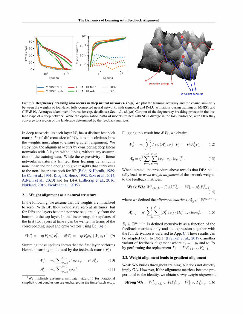
We explore to what extent degeneracy breaking occurs indeep nonlinear networks by training 4-layer multi-layerperceptrons (MLPs) with 100 nodes per layer for 1000epochs with both BP and DFA, on the MNIST and CIFAR10datasets, with Tanh and ReLU nonlinearities (cf. App. E.2for further experimental details). The dynamics of the train-ing loss, shown in the left of Fig. 5, are very similar for BPand DFA.

From degeneracy breaking, one expects DFA to drive the

2 3 4 5 6 7 8K

0.2

0.4

0.6

0.8

1.0

1.2

P(le

arn)

AnalyticalNumerical

t

g 0 pos1 pos2 pos

Figure 4. Over-parameterisation improves performance ofshallow ReLU networks. We show the learning dynamics ofa student with K = 3 hidden nodes trained on a teacher withM = 2 nodes and Wm

2 = 1 if the feedback vector has 0, 1, or2 positive entries. Inset: Probability of achieving zero test error(Eq. 8, line) compared to the fraction of simulations that con-verged to zero test error (out of 50, crosses). Other parameters:N = 500, η = 0.1, σ0 = 10−2.

optimization path towards a special region of the loss land-scape determined by the feedback matrices. We test thishypothesis by measuring whether networks trained withthe same feedback matrices from different initial weightsconverge towards the same region of the landscape. Thecosine similarity between the vectors obtained by stackingthe weights of two networks trained independently usingBP reaches at most 10−2 (right of Fig. 5), signalling thatthey reach very distinct minima. In contrast, when trainedwith DFA, networks reach a cosine similarity between 0.5and 1 at convergence, thereby confirming that DFA breaksthe degeneracy between the solutions in the landscape andbiases towards a special region of the loss landscape, bothfor sigmoidal and ReLU activation functions.

This result suggests that heavily over-parametrised neuralnetworks used in practice can be trained successfully withDFA because they have a large number of degenerate solu-tions. We leave a more detailed exploration of the interplaybetween DFA and the loss landscape for future work. Aswe discuss in Sec. 3 the Align-then-Memorise mechanismsketched in Fig. 3 c also occurs in deep non-linear networks.

2. How do gradients align in deep networks?This section focuses on the alignment phase of learning. Inthe two-layer setup there is a single feedback vector F1, ofsame dimensions as the second layer W2, and to which W2

must align in order for the first layer to recover the truegradient.


101 103

Epochs

0

20

40

60

80

Trai

n er

ror

101 103

Epochs

10 3

10 2

10 1

100

Cos

ine

sim

ilari

ty

MNIST reluMNIST tanh

CIFAR10 tanhCIFAR10 relu

DFABP

Figure 5. Degeneracy breaking also occurs in deep neural networks. (Left) We plot the training accuracy and the cosine similaritybetween the weights of four-layer fully-connected neural networks with sigmoidal and ReLU activations during training on MNIST andCIFAR10. Averages taken over 10 runs; for exp. details see Sec. 1.3. (Right) Cartoon of the degeneracy breaking process in the losslandscape of a deep network: while the optimization paths of models trained with SGD diverge in the loss landscape, with DFA theyconverge to a region of the landscape determined by the feedback matrices.

In deep networks, as each layer Wl has a distinct feedbackmatrix Fl of different size of Wl, it is not obvious howthe weights must align to ensure gradient alignment. Westudy how the alignment occurs by considering deep linearnetworks with L layers without bias, without any assump-tion on the training data. While the expressivity of linearnetworks is naturally limited, their learning dynamics isnon-linear and rich enough to give insights that carry overto the non-linear case both for BP (Baldi & Hornik, 1989;Le Cun et al., 1991; Krogh & Hertz, 1992; Saxe et al., 2014;Advani et al., 2020) and for DFA (Lillicrap et al., 2016;Nøkland, 2016; Frenkel et al., 2019).

2.1. Weight alignment as a natural structure

In the following, we assume that the weights are initialisedto zero. With BP, they would stay zero at all times, butfor DFA the layers become nonzero sequentially, from thebottom to the top layer. In the linear setup, the updates ofthe first two layers at time t can be written in terms of thecorresponding input and error vectors using Eq. (4)1:

δW t1 = −η(F1et)x

Tt , δW t

2 = −η(F2et)(W1xt)> (9)

Summing these updates shows that the first layer performsHebbian learning modulated by the feedback matrix F1:

W t1 = −η

∑t−1

t′=0F1et′x

>t′ = F1A

t1, (10)

At1 = −η∑t−1

t′=0et′x

>t′ (11)

1We implicitly assume a minibatch size of 1 for notationalsimplicity, but conclusions are unchanged in the finite-batch setup.

Plugging this result into δW t2 , we obtain:

W t2 = −η

t−1∑t′=0

F2et(At′

1 xt′)>F>1 = F2A

t2F>1 , (12)

At2 = η2t−1∑t′=0

t′−1∑t′′=0

(xt′ · xt′′)et′e>t′′ . (13)

When iterated, the procedure above reveals that DFA natu-rally leads to weak weight alignment of the network weightsto the feedback matrices:

Weak WA: W t1<l<L=FlA

tlF>l−1, W t

L=AtLF>L−1,

(14)

where we defined the alignment matrices Atl≥2 ∈ RnL×nL :

Atl≥2 = η2t−1∑t′=0

t′−1∑t′′=0

(Bt′

l xt′) · (Bt′′

l xt′′)et′e>t′′ . (15)

Bl ∈ RnL×nL is defined recursively as a function of thefeedback matrices only and its expression together withthe full derivation is deferred to App. C. These results canbe adapted both to DRTP (Frenkel et al., 2019), anothervariant of feedback alignment where et = −yt and to FAby performing the replacement Fl → FlFl+1 . . . FL−1.

2.2. Weight alignment leads to gradient alignment

Weak WA builds throughout training, but does not directlyimply GA. However, if the alignment matrices become pro-portional to the identity, we obtain strong weight alignment:

Strong WA: W t1<l<L ∝ FlF>l−1, W t

L ∝ F>L−1. (16)


101 103

Epochs

0.0

0.1

0.2

0.3

0.4

Wei

ght a

lignm

ent

101 103

Epochs

0.0

0.2

0.4

0.6

0.8

Gra

dien

t alig

nmen

t

MNIST reluMNIST tanhCIFAR10 tanhCIFAR10 relu

Figure 6. Global alignment dynamics of deep nonlinear net-works exhibits Align-then-Memorise. Global weight and gradi-ent alignments, as defined in (18), varying the activation functionand the dataset. Shaded regions represent the (small) variabilityover 10 runs.

Additionally, since GA requires Fle ∝W>l+1δal+1 (Eqs. 4and 2), strong WA directly implies GA if the feedback ma-trices Fl≥2 are assumed left-orthogonal, i.e. F>l Fl = InL

.Strong WA of (16) induces the weights, by the orthogonalitycondition, to cancel out by pairs of two:

W>l+1δal+1 ∝ FlF>l+1Fl+1 . . . F>L−1FL−1e = Fle. (17)

The above suggests that taking the feedback matrices left-orthogonal is favourable for GA. If the feedback matriceselements are sampled i.i.d. from a Gaussian distribution,GA still holds in expectation since E

[F>l Fl

]∝ InL

.

Quantifying gradient alignment Our analysis showsthat key to GA are the alignment matrices: the closer theyare to identity, i.e. the better their conditioning, the strongerthe GA. This comes at the price of restricted expressivity,since layers are encouraged to align to a product of (ran-dom) feedback matrices. In the extreme case of strong WA,the freedom of layers l ≥ 2 is entirely sacrificed to allowlearning in the first layer! This is not harmful for the lin-ear networks as the first layer alone is enough to maintainfull expressivity2. Nonlinear networks, as argued in Sec. 1,rely on the Degeneracy Breaking mechanism to recoverexpressivity.

3. The case of deep nonlinear networksIn this section, we show that the theoretical predictions ofthe previous two sections hold remarkably well in deepnonlinear networks trained on standard vision datasets.

3.1. Weight Alignment occurs like in the linear setup

To determine whether WA described in Sec. 2 holds in thedeep nonlinear setup of Sec. 1.3, we introduce the global

2such an alignment was indeed already observed in the linearsetup for BP (Ji & Telgarsky, 2019).

101 103

Epochs

0.0

0.2

0.4

0.6

0.8

Wei

ght a

lignm

ent

layer 2layer 3layer 4

101 103

Epochs

0.0

0.2

0.4

0.6

0.8

Gra

dien

t alig

nmen

t

layer 1layer 2layer 3

Figure 7. Layerwise alignment dynamics reveal sequentialAlign-then-Memorise. Layerwise weight and gradient align-ments as defined in (19), for a ReLU network trained on CIFAR10with 10% label corruption. Shaded regions represent the (small)variability over 10 runs.

and layerwise alignment observables:

WA=] (F,W), GA=](GDFA,GBP

)(18)

WAl≥2 =](Fl,Wl), GAl≥2 =](GDFAl ,GBP

l

), (19)

where ](A,B) = Vec(A) ·Vec(B)/‖A‖‖B‖ and

F =(F2F

>1 , . . . , FL−1F

>L−2, F

>L−1

),

W(t) =(W t

2 , . . . ,WtL−1,W

tL

),

G(t) =(δat1, . . . , δa

tL−1

).

Note that the layer-wise alignment of Wl with FlF>l−1 wasnever measured before: it differs from the alignment of Flwith Wl+1 . . .WL observed in (Crafton et al., 2019), whichis more akin to GA.

If W and F were uncorrelated, the WA defined in (18)would be vanishing as the width of the layer grows large.Remarkably, WA becomes of order one after a few epochsas shown in Fig. 6 (left), and strongly correlates with GA(right). This suggests that the layer-wise WA uncovered forlinear networks with weights initialized to zero also drivesGA in the general case.

3.2. Align-then-Memorise occurs from bottom layers totop

As can be seen in Fig. 6, WA clearly reaches a maximumthen decreases, as expected from the Align-then-Memoriseprocess. Notice that the decrease is stronger for CIFAR10than it is for MNIST, since CIFAR-10 is much harder to fitthan MNIST: more WA needs to be sacrificed. Increasinglabel corruption similarly makes the datasets harder to fit,and decreases the final WA, as detailed in SM E.2. However,another question arises: why does the GA keep increasingin this case, in spite of the decreasing WA?

To answer this question, we need to disentangle the dynam-ics of the layers of the network, as in Eq. (19). In Fig. 7,


0.2 0.4 0.6 0.8 1.0

0.2

0.4

0.6

0.8

1.0

Gradient alignment

Weight align

0.70

0.72

0.74

0.76

0.78

0.80

0.82

0.84

Figure 8. Badly conditioned output statistics can hamperalignment. WA and GA at the final point of training decreasewhen the output classes are correlated (β < 1) or of differentvariances (α < 1).

we focus on the ReLU network applied to CIFAR10, andshuffle 10% of the labels in the training set to make theAlign-then-Memorise procedure more easily visible. Al-though the network contains 4 layers of weights, we onlyhave 3 curves for WA and GA: WA is only defined for layers2 to 4 according to Eq. (19), whereas GA of the last layer isnot represented here since it is always equal to one.

As can be seen, the second layer is the first to start align-ing: it reaches its maximal WA around 1000 epochs (orangedashed line), then decreases. The third layer starts align-ing later and reaches its maximal WA around 2000 epochs(green dashed line), then decreases. As for the last layer,the WA is monotonically increasing. Hence, the Align-then-Memorise mechanism operates in a layerwise fashion,starting from the bottom layers to the top layers.

Note that the WA of the last layers is the most crucial, sinceit affects the GA of all the layers below, whereas the WAof the second layer only affects the GA of the first layer.It therefore makes sense to keep the WA of the last layershigh, and let the bottom layers perform the memorizationfirst. This is reminiscent of the linear setup, where all thelayers align except for the first, which does all the learning.In fact, this strategy enables the GA of each individual layerto keep increasing until late times: the diminishing WA ofthe bottom layers is compensated by the increasing WA ofthe top layers.

4. What can hamper alignment?We demonstrated that GA is enabled by the WA mechanism,both theoretically for linear networks and numerically fornonlinear networks. In this section, we leverage our analysisof WA to identify situations in which GA fails.

10 1 100 101 102

Epochs

0

20

40

60

80

Trai

n er

ror

p=0p=0.1p=0.2p=0.5p=0.9

10 1 100 101 102

Epochs

0.0

0.2

0.4

0.6

0.8

Gra

dien

t alig

nmen

t

Weight align

Figure 9. Label corruption hampers alignment in the earlystages of training. We see that the higher the label corruption, themore time WA and GA take to start increasing, since the networkinitially predicts equal probabilities over the output classes.

4.1. Alignment is data-dependent

In the linear case, GA occurs if the alignment matrices pre-sented in Sec. 2 are well conditioned. Note that if the outputsize nL is equal to one, e.g. for scalar regression or binaryclassification tasks, then the alignment matrices are simplyscalars, and GA is guaranteed. When this is not the case,one can obtain the deviation from GA by studying the ex-pression of the alignment matrices (15). They are formed bysumming outer products of the error vectors et′e>t′′ , whereet = yt−yt. Therefore, good conditioning requires thedifferent components of the errors to be uncorrelated and ofsimilar variances. This can be violated by (i) the targets y,or (ii) the predictions y.

(i) Structure of data The first scenario can be demon-strated in a simple regression task on i.i.d. Gaussian inputsx ∼ R10. The targets y ∈ R2 are randomly sampled fromthe following distribution:

y∼N (0,Σ), Σ=

(1 α(1− β)

α(1− β) α2

), α, β≤ 1.

(20)

In Fig. 8, we show the final WA and GA of a 3-layer ReLUnetwork trained for 103 epochs on 103 examples sampledfrom this distribution (further details in SM E.3). As pre-dicted, imbalanced (α < 1) or correlated (β < 1) targetstatistics hamper WA and GA. Note that the inputs alsocome into play in Eq. (15): a more detailed theoretical anal-ysis of the impact of input and target statistics on alignmentis deferred to SM D.

(ii) Effect of noise For classification tasks, the targets yare one-hot encodings whose statistics are naturally wellconditioned. However, alignment can be degraded if thestatistics of the predictions y become correlated.

One can enforce such a correlation in CIFAR10 by shufflinga fraction p of the labels. The WA and GA dynamics ofa 3-layer ReLU network are shown in Fig. 9. At high p,


the network can only perform random guessing during thefirst few epochs, and assigns equal probabilities to the 10classes. The correlated structure of the predictions preventsalignment until the network starts to fit the random labels:the predictions of the different classes then decouple andWA takes off, leading to GA.

4.2. Alignment is impossible for convolutional layers

A convolutional layer with filters Hl can be represented bya large fully-connected layer whose weights are representedby a block Toeplitz matrix φ(Hl) (d’Ascoli et al., 2019).This matrix has repeated blocks due to weight sharing, andmost of its weights are equal to zero due to locality. Inorder to verify WA and therefore GA, the following con-dition must hold: φ(Hl) ∝ FlF

>l−1. Yet, due to the very

constrained structure of φ(Hl), this is impossible for a gen-eral choice of Fl. Therefore, the WA mechanism suggestsa simple explanation for why GA doesn’t occur in vanillaCNNs, and confirms the previously stated hypothesis thatCNNs don’t have enough flexibility to align (Launay et al.,2019).

In the case of convolutional layers, this lack of alignmentmakes learning near to impossible, and has lead practition-ers to design alternatives (Han & Yoo, 2019; Moskovitzet al., 2018). However, the extent to which alignment corre-lates with good performance in the general setup (both interms of fitting and generalisation) is a complex questionwhich we leave for future work. Indeed, nothing preventsDFA from finding a good optimization path, different fromthe one followed by BP. Conversely, obtaining high gradientalignment at the end of training is not a sufficient condi-tion for DFA to retrieve the results of BP, e.g. if the initialtrajectory leads to a wrong direction.

AcknowledgementsWe thank Florent Krzakala for introducing us to feedbackalignment, and we thank him and Lenka Zdeborova fororganising the Les Houches 2020 workshop on Statisti-cal Physics and Machine Learning where this work wasinitiated. We thank Florent Krzakala, Giulio Biroli, Char-lotte Frenkel, Julien Launay, Martin Lefebvre, LeonardoPetrini, Iacopo Poli, Levent Sagun and Mihiel Straat forhelpful discussions. MR acknowledges funding from theFrench Agence Nationale de la Recherche under grant ANR-19-P3IA-0001 PRAIRIE. SD acknowledges funding fromPRAIRIE for a visit to Trieste to collaborate on this project.RO acknowledges funding from the Region Ile-de-France.

ReferencesAdvani, M. S., Saxe, A. M., and Sompolinsky, H. High-

dimensional dynamics of generalization error in neural

networks. Neural Networks, 132:428 – 446, 2020.

Aubin, B., Maillard, A., Barbier, J., Krzakala, F., Macris,N., and Zdeborova, L. The committee machine: Compu-tational to statistical gaps in learning a two-layers neuralnetwork. In Advances in Neural Information ProcessingSystems 31, pp. 3227–3238, 2018.

Bahri, Y., Kadmon, J., Pennington, J., Schoenholz, S., Sohl-Dickstein, J., and Ganguli, S. Statistical Mechanics ofDeep Learning. Annual Review of Condensed MatterPhysics, 11(1):501–528, 2020.

Baity-Jesi, M., Sagun, L., Geiger, M., Spigler, S., Arous,G., Cammarota, C., LeCun, Y., Wyart, M., and Biroli,G. Comparing Dynamics: Deep Neural Networks versusGlassy Systems. In Proceedings of the 35th InternationalConference on Machine Learning, 2018.

Baldi, P. and Hornik, K. Neural networks and principalcomponent analysis: Learning from examples withoutlocal minima. Neural networks, 2(1):53–58, 1989.

Bartunov, S., Santoro, A., Richards, B., Marris, L., Hin-ton, G. E., and Lillicrap, T. Assessing the scalabilityof biologically-motivated deep learning algorithms andarchitectures. In Advances in Neural Information Pro-cessing Systems, pp. 9368–9378, 2018.

Biehl, M. and Schwarze, H. Learning by on-line gradientdescent. J. Phys. A. Math. Gen., 28(3):643–656, 1995.

Brutzkus, A. and Globerson, A. Globally optimal gradientdescent for a convnet with gaussian inputs. In Proceed-ings of the 34th International Conference on MachineLearning - Volume 70, ICML’17, pp. 605–614, 2017.

Chizat, L. and Bach, F. On the global convergence of gradi-ent descent for over-parameterized models using optimaltransport. In Advances in Neural Information ProcessingSystems 31, pp. 3040–3050, 2018.

Crafton, B., Parihar, A., Gebhardt, E., and Raychowdhury,A. Direct feedback alignment with sparse connections forlocal learning. Frontiers in neuroscience, 13:525, 2019.

Crick, F. The recent excitement about neural networks.Nature, 337(6203):129–132, 1989.

d’Ascoli, S., Sagun, L., Biroli, G., and Bruna, J. Finding theneedle in the haystack with convolutions: on the benefitsof architectural bias. In Advances in Neural InformationProcessing Systems, pp. 9334–9345, 2019.

Du, S., Lee, J., Tian, Y., Singh, A., and Poczos, B. Gradientdescent learns one-hidden-layer CNN: Don’t be afraid ofspurious local minima. In Proceedings of the 35th Inter-national Conference on Machine Learning, volume 80,pp. 1339–1348, 2018.


Engel, A. and Van den Broeck, C. Statistical mechanics oflearning. Cambridge University Press, 2001.

Frenkel, C., Lefebvre, M., and Bol, D. Learning withoutfeedback: Direct random target projection as a feedback-alignment algorithm with layerwise feedforward training.2019.

Gabrie, M. Mean-field inference methods for neural net-works. Journal of Physics A: Mathematical and Theoreti-cal, 53(22):223002, 2020.

Gardner, E. and Derrida, B. Three unfinished works on theoptimal storage capacity of networks. Journal of PhysicsA: Mathematical and General, 22(12):1983–1994, 1989.

Ghorbani, B., Mei, S., Misiakiewicz, T., and Montanari, A.Limitations of lazy training of two-layers neural network.In Advances in Neural Information Processing Systems32, pp. 9111–9121, 2019.

Gilmer, J., Raffel, C., Schoenholz, S. S., Raghu, M., andSohl-Dickstein, J. Explaining the learning dynamics of di-rect feedback alignment. In ICLR workshop track, 2017.

Goldt, S., Advani, M., Saxe, A., Krzakala, F., and Zde-borova, L. Dynamics of stochastic gradient descent fortwo-layer neural networks in the teacher-student setup.In Advances in Neural Information Processing Systems32, 2019.

Grossberg, S. Competitive learning: From interactive acti-vation to adaptive resonance. Cognitive science, 11(1):23–63, 1987.

Han, D. and Yoo, H.-j. Direct feedback alignment based con-volutional neural network training for low-power onlinelearning processor. In Proceedings of the IEEE Interna-tional Conference on Computer Vision Workshops, 2019.

Ji, Z. and Telgarsky, M. Gradient descent aligns the layersof deep linear networks. In International Conference onLearning Representations (ICLR), 2019.

Kinzel, W. and Rujan, P. Improving a Network Generaliza-tion Ability by Selecting Examples. EPL (EurophysicsLetters), 13(5):473–477, 1990.

Krogh, A. and Hertz, J. A. Generalization in a linear per-ceptron in the presence of noise. Journal of Physics A:Mathematical and General, 25(5):1135, 1992.

Launay, J., Poli, I., and Krzakala, F. Principled train-ing of neural networks with direct feedback alignment.arXiv:1906.04554, 2019.

Launay, J., Poli, I., Boniface, F., and Krzakala, F. Directfeedback alignment scales to modern deep learning tasksand architectures. In Advances in neural informationprocessing systems, 2020.

Le Cun, Y., Kanter, I., and Solla, S. A. Eigenvalues of covari-ance matrices: Application to neural-network learning.Physical Review Letters, 66(18):2396, 1991.

Liao, Q., Leibo, J. Z., and Poggio, T. How important isweight symmetry in backpropagation? In Proceedings ofthe Thirtieth AAAI Conference on Artificial Intelligence,pp. 1837–1844, 2016.

Lillicrap, T., Cownden, D., Tweed, D., and Akerman, C.Random synaptic feedback weights support error back-propagation for deep learning. Nature Communications,7:1–10, 2016.

Mei, S., Montanari, A., and Nguyen, P. A mean field view ofthe landscape of two-layer neural networks. Proceedingsof the National Academy of Sciences, 115(33):E7665–E7671, 2018.

Moskovitz, T. H., Litwin-Kumar, A., and Abbott, L. Feed-back alignment in deep convolutional networks. arXivpreprint arXiv:1812.06488, 2018.

Nøkland, A. Direct Feedback Alignment Provides Learn-ing in Deep Neural Networks. In Advances in NeuralInformation Processing Systems 29, 2016.

Rotskoff, G. and Vanden-Eijnden, E. Parameters as inter-acting particles: long time convergence and asymptoticerror scaling of neural networks. In Advances in Neu-ral Information Processing Systems 31, pp. 7146–7155,2018.

Rumelhart, D. E., Hinton, G. E., and Williams, R. J. Learn-ing representations by back-propagating errors. Nature,323(6088):533–536, 1986.

Saad, D. On-line learning in neural networks, volume 17.Cambridge University Press, 2009.

Saad, D. and Solla, S. Exact Solution for On-Line Learningin Multilayer Neural Networks. Phys. Rev. Lett., 74(21):4337–4340, 1995a.

Saad, D. and Solla, S. On-line learning in soft committeemachines. Phys. Rev. E, 52(4):4225–4243, 1995b.

Saxe, A., McClelland, J., and Ganguli, S. Exact solutionsto the nonlinear dynamics of learning in deep linear neu-ral networks. In International Conference on LearningRepresentations (ICLR), 2014.

Saxe, A., Bansal, Y., Dapello, J., Advani, M., Kolchinsky,A., Tracey, B., and Cox, D. On the information bottlenecktheory of deep learning. In ICLR, 2018.

Seung, H. S., Sompolinsky, H., and Tishby, N. Statisticalmechanics of learning from examples. Physical ReviewA, 45(8):6056–6091, 1992.


Sirignano, J. and Spiliopoulos, K. Mean field analysis ofneural networks: A central limit theorem. StochasticProcesses and their Applications, 2019.

Soltanolkotabi, M., Javanmard, A., and Lee, J. Theoret-ical insights into the optimization landscape of over-parameterized shallow neural networks. IEEE Trans-actions on Information Theory, 65(2):742–769, 2018.

Tian, Y. An analytical formula of population gradient fortwo-layered relu network and its applications in con-vergence and critical point analysis. In Proceedings ofthe 34th International Conference on Machine Learning(ICML), pp. 3404–3413, 2017.

Watkin, T., Rau, A., and Biehl, M. The statistical mechanicsof learning a rule. Reviews of Modern Physics, 65(2):499–556, 1993.

Yoshida, Y. and Okada, M. Data-dependence of plateauphenomenon in learning with neural network — statisticalmechanical analysis. In Advances in Neural InformationProcessing Systems 32, pp. 1720–1728, 2019.

Zdeborova, L. and Krzakala, F. Statistical physics of in-ference: thresholds and algorithms. Adv. Phys., 65(5):453–552, 2016.

Zhong, K., Song, Z., Jain, P., Bartlett, P., and Dhillon, I. Re-covery guarantees for one-hidden-layer neural networks.In Proceedings of the 34th International Conference onMachine Learning-Volume 70, pp. 4140–4149, 2017.


A. Derivation of the ODEThe derivation of the ODE’s that describe the dynamics ofthe test error for shallow networks closely follows the oneof Saad & Solla (1995a) and Biehl & Schwarze (1995) forback-propagation. Here, we give the main steps to obtainthe analytical curves of the main text and refer the reader totheir paper for further details.

As we discuss in Sec. 1, student and teacher are both two-layer networks with K and M hidden nodes, respectively.For an input x ∈ RN , their outputs y and y can be writtenas

y = φθ(x) =

K∑k=1

W k2 g(λk),

y = φθ(x) =

M∑m=1

Wm2 g (νm) , (21)

where we have introduced the pre-activations λk ≡W k

1 x/√N and νm ≡ Wm

1 x/√N . Evaluating the test error

of a student with respect to the teacher under the squaredloss leads us to compute the average

εg

(θ, θ)

=1

2E x

[K∑k=1

W k2 g(λk)−

M∑m=1

Wm2 g (νm)

]2,

(22)where the expectation is taken over inputs x for a fixedstudent and teacher. Since x only enters Eq. (22) via thepre-activations λ = (λk) and ν = (νm), we can replace thehigh-dimensional average over x by a low-dimensional av-erage over the K +M variables (λ, ν). The pre-activationsare jointly Gaussian since the inputs are drawn element-wisei.i.d. from the Gaussian distribution. The mean of (λ, ν) iszero since Exi = 0, so the distribution of (λ, ν) is fullydescribed by the second moments

Qkl = Eλkλl = W k1 ·W l

1/N, (23)

Rkm = Eλkνm = W k1 · Wm

1 /N, (24)

Tmn = E νmνn = Wm1 · Wn

1 /N. (25)

which are the “order parameters” that we introduced in themain text. We can thus rewrite the generalisation error (5) asa function of only the order parameters and the second-layerweights,

limN→∞

εg(θ, θ) = εg(Q,R, T,W2, W2) (26)

As we update the weights using SGD, the time-dependentorder parameters Q,R, and W2 evolve in time. By choos-ing different scalings for the learning rates in the SGD up-dates (4), namely

ηW1 = η, ηW2 = η/N

for some constant η, we guarantee that the dynamics ofthe order parameters can be described by a set of ordinarydifferential equations, called their “equations of motion”.We can obtain these equations in a heuristic manner bysquaring the weight update (4) and taking inner productswith Wm

1 , to yield the equations of motion for Q and Rrespectively:

dRkm

dα= −ηF k1 E

[g′(λk)νme

](27a)

dQk`

dα= −ηF k1 E

[g′(λk)λ`e

]− ηF `1E

[g′(λ`)λke

]+ η2F k1 F

`1E[g′(λk)g′(λ`)e2

], (27b)

dW k2

dα= −ηE

[g(λk)e

](27c)

where, as in the main text, we introduced the error e =φθ(x)−φθ(x). In the limitN →∞, the variable α = µ/Nbecomes a continuous time-like variable. The remainingaverages over the pre-activations, such as

E g′(λk)λ`g(νm),

are simple three-dimensional integral over the Gaussianrandom variables λk, λ` and νm and can be evaluated an-alytically for the choice of g(x) = erf(x/

√2) (Biehl &

Schwarze, 1995) and for linear networks with g(x) = x.Furthermore, these averages can be expressed only in termof the order parameters, and so the equations close. Wenote that the asymptotic exactness of Eqs. 27 can be provenusing the techniques used recently to prove the equations ofmotion for BP (Goldt et al., 2019).

We provide an integrator for the full system of ODEs forany K and M in the Github repository.

B. Detailed analysis of DFA dynamicsIn this section, we present a detailed analysis of the ODE dy-namics in the matched case K = M for sigmoidal networks(g(x) = erf (x/

√2)).

The Early Stages and Gradient Alignment We now useEqs. (27) to demonstrate that alignment occurs in the earlystages of learning, determining from the start the solutionDFA will converge to (see Fig. 3 which summarises thedynamical evolution of the student’s second layer weights).

Assuming zero initial weights for the student and orthogonalfirst layer weights for the teacher (i.e. Tnm is the identitymatrix), for small times (t� 1), one can expand the orderparameters in t:

Rkm(t) = tRkm(0) +O(t2),

Qkl(t) = tQkl(0) +O(t2),

W k2 (t) = tW k

2 (0) +O(t2). (28)


where, due to the initial conditions, R(0) = Q(0) =W2(0) = 0. Using Eq. 27, we can obtain the lowest or-der term of the above updates:

Rkm(0) =

√2

πηWm

2 Fk1 ,

Qkl(0) =2

πη2(

(W k2 )2 + (W l

2)2)F l1F

k1 ,

W k2 (0) = 0 (29)

Since both R(0) and Q(0) are non-zero, this initial condi-tion is not a fixed point of DFA. To analyse initial alignment,we consider the first order term of W2. Using Eq. (28) withthe derivatives at t = 0 (29), we obtain to linear order in t:

W k2 (t) =

2

π2η2||W2||2F k1 t. (30)

Crucially, this update is in the direction of the feedback vec-tor F1. DFA training thus constrains the student to initiallygrow in the direction of the feedback vector and align withit. This implies gradient alignment between BP and DFAand dictates into which of the many degenerate solutions inthe energy landscape the student converges.

Plateau phase After the initial phase of learning withDFA where the test error decreases exponentially, similarlyto BP, the student falls into a symmetric fixed point of theEqs. (27) where the weights of a single student node arecorrelated to the weights of all the teacher nodes ((Saad &Solla, 1995a; Biehl & Schwarze, 1995; Engel & Van denBroeck, 2001)). The test error stays constant while thestudent is trapped in this fixed point. We can obtain ananalytic expression for the order parameters under the as-sumption that the teacher first-layer weights are orthogonal(Tnm = δnm). We set the teacher’s second-layer weightsto unity for notational simplicity (Wm

2 = 1) and restrict tolinear order in the learning rate η, since this is the dominantcontribution to the learning dynamics at early times and onthe plateau (Saad & Solla, 1995b). In the case where allcomponents of the feedback vector are positive, the orderparameters are of the form Qkl = q,Rkm = r,W k

2 = w2

with:

q =1

2K − 1, r =

√q

2, w2 =

√1 + 2q

q(4 + 3q). (31)

If the components of the feedback vector are not all positive,we instead obtain Rkm = sgn(F k)r, W k

2 = sgn(F k)w2

and Qkl = sgn(F k) sgn(F l)q. This shows that on theplateau the student is already in the configuration that max-imises its alignment with F1. Note that in all cases, thevalue of the test error reached at the plateau is the same forDFA and BP.

Memorisation phase and Asymptotic Fixed Point Atthe end of the plateau phase, the student converges to itsfinal solution, which is often referred to as the specialisedphase (Saad & Solla, 1995a; Biehl & Schwarze, 1995; Engel& Van den Broeck, 2001). The configuration of the orderparameters is such that the student reproduces her teacherup to sign changes that guarantee the alignment betweenW2 and F1 is maximal, i.e. sgn(W k

2 ) = sgn(F k1 ). Thefinal value of the test error of a student trained with DFA isthe same as that of a student trained with BP on the sameteacher.

100 102 104 106

t10 4

10 3

10 2

10 1

100

g

RandomOrthogonal

Figure 10. Test error of a sigmoidal student started with zero initialweights. The feedback vector F1 is chosen random (blue) andorthogonal to the teacher’s second layer weights W2 (orange).Parameters: η = 0.1,K =M = 2.

Choice of the feedback vector In the main text, we sawhow a wrong choice of feedback vector F1 can prevent aReLU student from learning a task. Here, we show that alsofor sigmoidal student, a wrong choice of feedback vectorF1 is possible. As Fig. 10 shows, in the case where the F1

is taken orthogonal to the teacher second layer weights, astudent whose weights are initialised to zero remains stuckon the plateau and is unable to learn. In contrast, when theF1 is chosen with random i.i.d. components drawn from thestandard normal distribution, perfect recovery is achieved.

C. Derivation of weight alignmentSince the network is linear, the update equations are (con-sider the first three layers only):

δW1 = −η(F1e)xT , (32)

δW2 = −η(F2e)(W1x)>, (33)

δW3 = −η(F3e)(W2W1x)> (34)


First, it is straightforward to see that

W t1 = −η

t−1∑t′=0

F1et′x>t′ = F1A

t1 (35)

At1 = −ηt−1∑t′=0

et′x>t′ (36)

This allows to calculate the dynamics of W t2 :

δW t2 = −ηF2et(A

t1xt)

>F>1 (37)

W t2 = −η

t−1∑t′=0

F2et(At′

1 xt′)>F>1 = F2A

t2F>1 (38)

At2 = −ηt−1∑t′=0

et′(At′

1 xt′)> = η2

t−1∑t′=0

t′−1∑t′′=0

(xt′ · xt′′)et′e>t′′ .

(39)

Which in turns allows to calculate the dynamics of W t3 :

δW t3 = −ηF3et(F2A

t′

2 F>1 F1A

t′

1 xt)> (40)

W t3 = −η

t−1∑t′=0

F3et′(F2At′

2 F>1 F1A

t′

1 xt)> = F3A

t3F>2

(41)

At3 = −ηt−1∑t′=0

F3et′(At′

2 F>1 F1A

t′

1 xt′)> (42)

= η2t−1∑t′=0

t′−1∑t′′=0

(At′

1 xt′) · (At′′

1 xt′′)et′e>t′′ . (43)

By induction it is easy to show the general expression:

At1 = −ηt−1∑t′=0

et′x>t′ (44)

At2 = η2t−1∑t′=0

t′−1∑t′′=0

(xt′ · xt′′)et′e>t′′ (45)

Atl≥3 = η2∑t,t′=0

(At′

l−2 . . . At′

1 xt′) · (At′′

l−2 . . . At′′

1 xt′′)et′e>t′′

(46)

Defining A0 ≡ In0, one can rewrite this as in Eq. 15

Atl≥2 = η2t−1∑t′=0

t′−1∑t′′=0

(Bt′

l xt′) · (Bt′′

l xt′′)et′e>t′′ , (47)

Bl = Al−2 · · ·A0. (48)

D. Impact of data structureTo study the impact of data structure on the alignment, thesimplest setup to consider is that of Direct Random Target

Projection (Frenkel et al., 2019). Indeed, in this case theerror vector et = −yt does not depend on the prediction ofthe network: the dynamics become explicitly solvable in thelinear case.

For concreteness, we consider the setup of (Lillicrap et al.,2016) where the targets are given by a linear teacher, y =Tx, and the inputs are i.i.d Gaussian. We denote the inputand target correlation matrices as follows:

E[xx>

]≡ Σx ∈ Rn0×n0 , (49)

E[TT>

]≡ Σy ∈ RnL×nL (50)

If the batch size is large enough, one can write xtx>t =E[xx>

]= Σx. Hence the dynamics of Eq. 9 become:

δW t1 = −η(F1et)x

Tt = ηF1Txtx

>t = ηF1TΣx (51)

δW t2 = −η(F2et)(W1xt)

>= ηF2TΣxW

>1 (52)

= η2F2

(TΣ2

xT>)F>1 (53)

δW t3 = −η(F3et)(W2W1xt)

>= ηF3TΣxW

>1 W

>2

(54)

= η3F3

(TΣ2

xT>) (TΣ2

xT>)F>2 (55)

From which we easily deduce At1 = ηTΣxt, and the expres-sion of the alignment matrices at all times:

Atl≥2 = ηl(TΣ2

xT>)l−1 t (56)

As we saw, GA depends on how well-conditioned the aligne-ment matrices are, i.e. how different it is from the identity.To examine deviation from identity, we write Σx = In0

+Σxand Σy = InL

+ Σy , where the tilde matrices are small per-turbations. Then to first order,

Atl≥2 − InL∝ (l − 1)

(Σy + 2T ΣxT

>)

(57)

Here we see that GA depends on how well-conditioned theinput and target correlation matrices Σx and Σy are. Inother words, if the different components of the inputs or thetargets are correlated or of different variances, we expectGA to be hampered, observed in Sec. 4. Note that due tothe l − 1 exponent, we expect poor conditioning to have aneven more drastic effect in deeper layers.

Notice that in this DRTP setup, the norm of the weightsgrows linearly with time, which makes DRTP inapplicableto regression tasks, and over-confident in classification tasks.It is clear in this case the the first layer learns the teacher, andthe subsequent layers try to passively transmit the signal.

E. Details about the experimentsE.1. Direct Feedback Alignment implementation

We build on the Pytorch implementation of DFAimplemented in (Launay et al., 2020), accessi-


ble at https://github.com/lightonai/dfa-scales-to-modern-deep-learning/tree/master/TinyDFA. Note that we do not use theshared feedback matrix trick introduced in this work. Wesample the elements of the feedback matrix Fl from acentered uniform distribution of scale 1/

√nl + 1.

E.2. Experiments on realistic datasets

We trained 4-layer MLPs with 100 nodes per layer for 1000epochs using vanilla SGD, with a batch size of 32 and alearning rate of 10−4. The datasets considered are MNISTand CIFAR10, and the activation functions are Tanh andReLU.

We initialise the networks using the standard Pytorch ini-tialization scheme. We do not use any momentum, weightdecay, dropout, batchnorm or any other bells and whistles.We downscale all images to 14× 14 pixels to speed up theexperiments. Results are averaged over 10 runs.

For completeness, we show in Fig. 11 the results in the maintext for 4 different levels of label corruption. The transitionfrom Alignment phase to Memorisation phase can clearly beseen in all cases from the drop in weight alignment. Threeimportant remarks can be made:

• Alignment phase: Increasing label corruption slowsdown the early increase of weight alignment, as notedin Sec. 4.1.

• Memorization phase: Increasing label corruptionmakes the datasets harder to fit. As a consequence,the network needs to give up more weight alignmentin the memorization phase, as can be seen from thesharper drop in the weight alignment curves.

• Transition point: the transition time between theAlignement and Memorization phases coincides withthe time at which the training error starts to decreasesharply (particularly at high label corruption), and ishardly affected by the level of label corruption.

E.3. Experiment on the structure of targets

We trained a 3-layer linear MLP of width 100 for 1000epochs on the synthetic dataset described in the main text,containing 104 examples. We used the same hyperparame-ters as for the experiment on nonlinear networks. We choose5 values for α and β: 0.2, 0.4, 0.6, 0.8 and 1.

In Fig. 12, we show the dynamics of weight alignment forboth ReLU and Tanh activations. We again see the Align-then-Memorise process distinctly. Notice that decreasing αand β hampers both the mamixmal weight alignment (at theend of the alignment phase) and the final weight alignment(at the end of the memorisation phase).

https://github.com/lightonai/dfa-scales-to-modern-deep-learning/tree/master/TinyDFA




101 103

Epochs

0

20

40

60

80

Trai

n er

ror

A

101 103

Epochs

0.0

0.1

0.2

0.3

0.4

Wei

ght a

lignm

ent

B

101 103

Epochs

0.0

0.2

0.4

0.6

0.8

Gra

dien

t alig

nmen

t

C

101 103

Epochs

10 3

10 2

10 1

100

Cos

ine

sim

ilari

ty

D

MNIST reluMNIST tanhCIFAR10 tanhCIFAR10 reluDFABP

(a) No label corruption

101 103

Epochs

0

20

40

60

80

Trai

n er

ror

A

101 103

Epochs

0.0

0.1

0.2

0.3

0.4

Wei

ght a

lignm

ent

B

101 103

Epochs

0.0

0.2

0.4

0.6

0.8

Gra

dien

t alig

nmen

t

C

101 103

Epochs

10 4

10 3

10 2

10 1

100

Cos

ine

sim

ilari

ty

D

MNIST reluMNIST tanhCIFAR10 reluCIFAR10 tanhDFABP

(b) 50% label corruption

101 103

Epochs

0

20

40

60

80

Trai

n er

ror

A

101 103

Epochs

0.0

0.1

0.2

0.3

0.4

Wei

ght a

lignm

ent

B

101 103

Epochs

0.0

0.2

0.4

0.6

0.8

Gra

dien

t alig

nmen

t

C

101 103

Epochs

10 4

10 3

10 2

10 1

Cos

ine

sim

ilari

ty

D

MNIST reluCIFAR10 reluMNIST tanhCIFAR10 tanhDFABP

(c) 90% label corruption

Figure 11. Effect of label corruption on training observables. A: Training error. B and C: Weight and gradient alignment, as defined in themain text. D: Cosine similarity of the weight during training.


0.2 0.4 0.6 0.8 1.0

0.2

0.4

0.6

0.8

1.0

Gradient alignment

Weight align

0.70

0.72

0.74

0.76

0.78

0.80

0.82

0.84

102 104

Epochs

0.0

0.1

0.2

Wei

ght a

lignm

ent

= 0.2

102 104

Epochs

= 0.6

102 104

Epochs

= 1.0

= 0.2= 0.4= 0.6= 0.8= 1.0

(a) ReLU

0.2 0.4 0.6 0.8 1.0

0.2

0.4

0.6

0.8

1.0

Gradient alignment

Weight align

0.64

0.66

0.68

0.70

0.72

0.74

0.76

0.78

0.80

102 104

Epochs

0.0

0.1

0.2

Wei

ght a

lignm

ent

= 0.2

102 104

Epochs

= 0.6

102 104

Epochs

= 1.0

= 0.2= 0.4= 0.6= 0.8= 1.0

(b) Tanh

Figure 12. WA is hampered when the output dimensions are correlated (β < 1) or of different variances (α < 1).

align, then memorise: the dynamics of learning with

Documents