all-at-once optimization for mining higher-order tensors · all-at-once optimization for mining...
TRANSCRIPT
All-at-once Optimization for Mining
Higher-order Tensors
Evrim Acar
Tamara G. Kolda, Sandia National Labs, Livermore, CA
Daniel M. Dunlavy, Sandia National Labs, Albuquerque, NM
Faculty of Life Sciences
University of Copenhagen

Matrix Factorizations
in Data Mining
Capturing
underlying
hidden factors≈
…use
rs
terms
+topic 1 topic 2 topic R

Matrix Factorizations
in Data Mining
Capturing
underlying
hidden factors≈
…use
rs
terms
+topic 1 topic 2 topic R
Incomplete
Matrix
Factorization/
Matrix
Completion
≈…
mo
vie
s
customers
+≈

Matrix Factorizations
in Data Mining
Capturing
underlying
hidden factors≈
…use
rs
terms
+topic 1 topic 2 topic R
Incomplete
Matrix
Factorization/
Matrix
Completion
Collective
Matrix
Factorization
≈…
mo
vie
s
customers
+≈
mov
ies
customers
≈m
ov
ies
customers
mo
vie
s
actors

Data sets are often multi-modal…
Capturing
underlying
hidden factors
≈
conversation 1
Incomplete
Tensor
Factorization
/Tensor
Completion
Coupled
Matrix-Tensor
Factorization
use
rs
terms
+ …
conversation 2 conversation R
≈
cust
om
ers
items
≈
≈
cust
om
ers
items
time
cust
om
ers
itemslocations
cust
om
ers
locations
+ …
=I
K
R components
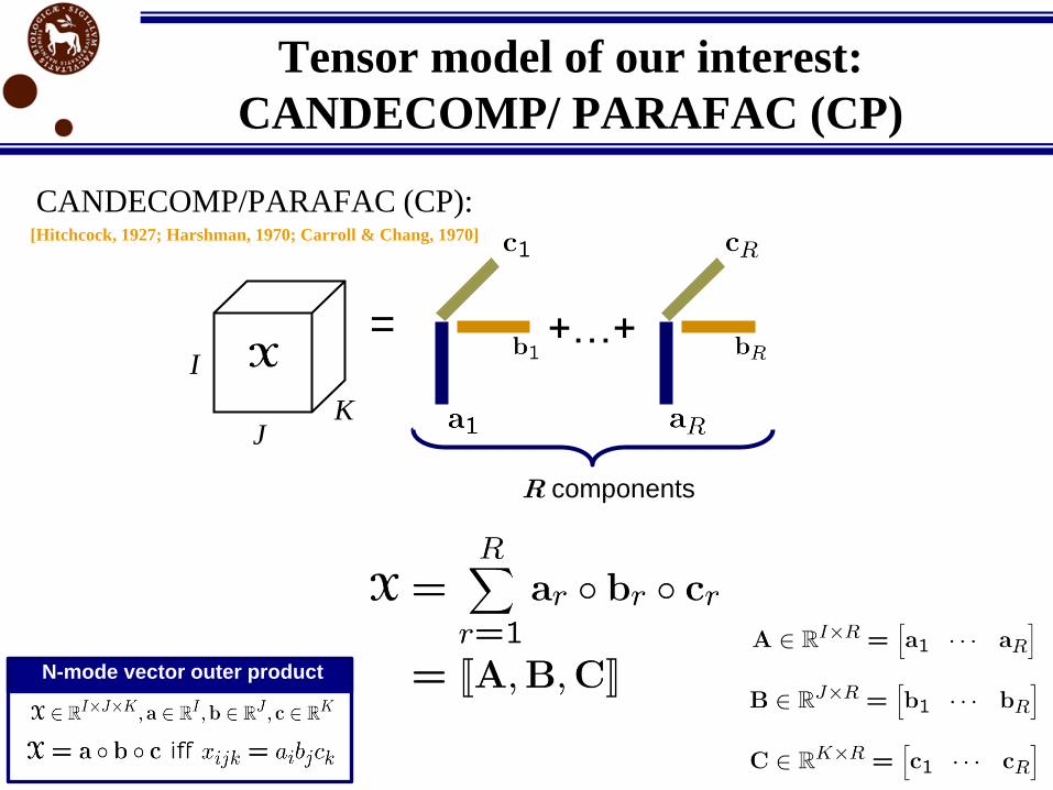
Tensor model of our interest:
CANDECOMP/ PARAFAC (CP)
J
CANDECOMP/PARAFAC (CP): [Hitchcock, 1927; Harshman, 1970; Carroll & Chang, 1970]
N-mode vector outer product
+…+
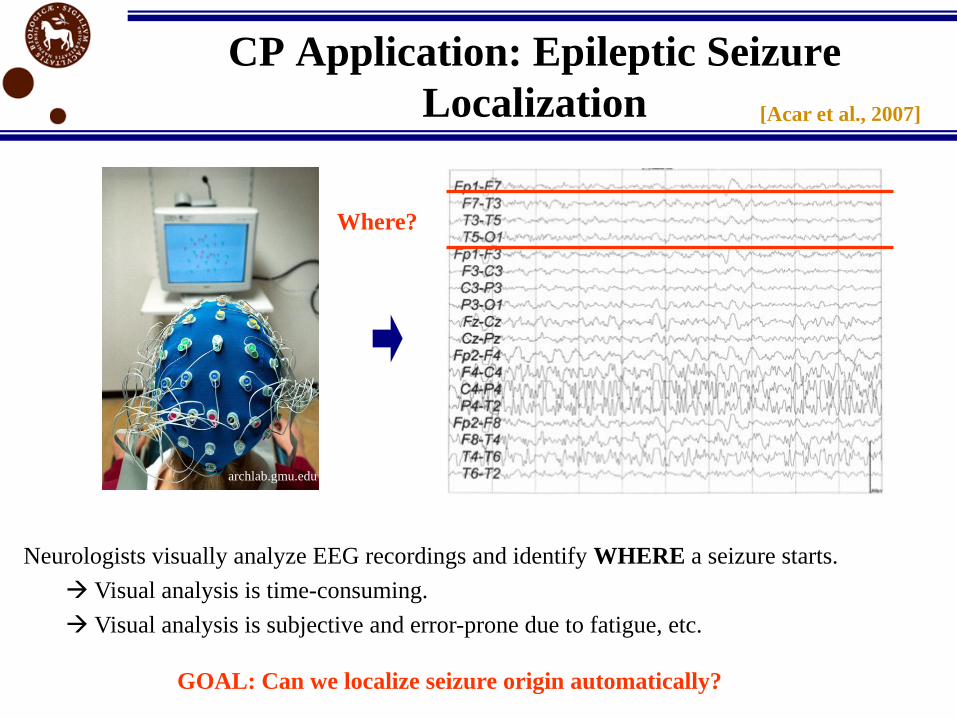
CP Application: Epileptic Seizure
Localization
Neurologists visually analyze EEG recordings and identify WHERE a seizure starts.
Visual analysis is time-consuming.
Visual analysis is subjective and error-prone due to fatigue, etc.
GOAL: Can we localize seizure origin automatically?
Where?
archlab.gmu.edu
[Acar et al., 2007]

Epilepsy Tensors
Ch
an
nel
s
Time
Tim
e sa
mp
les
Channels Scales (freq.)
Channels
Tim
e sa
mp
lesCWT
CWT
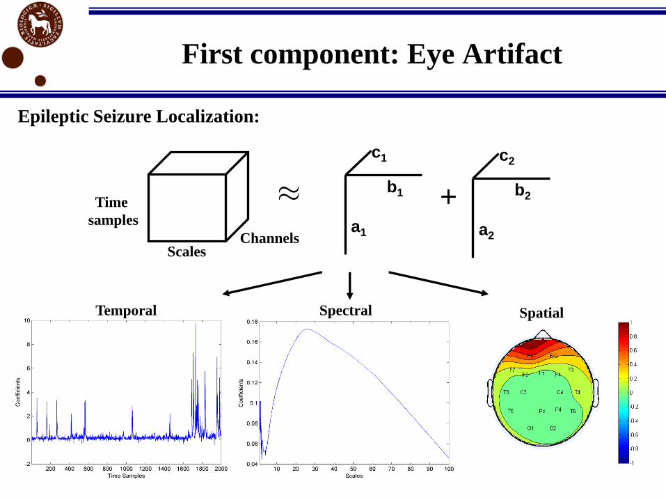
First component: Eye Artifact
Time
samples
Scales Channels
+a1
b1
c1
a2
b2
c2
Epileptic Seizure Localization:
Temporal Spectral Spatial
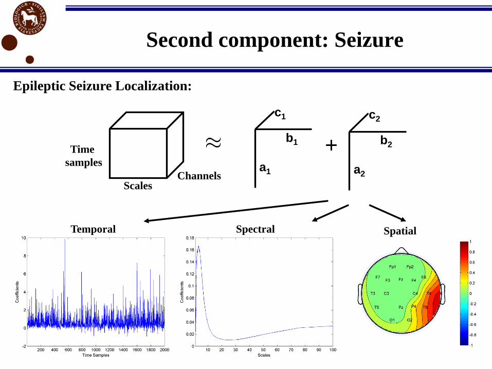
Second component: Seizure
Scales Channels
+a1
b1
c1
a2
b2
c2
Epileptic Seizure Localization:
Temporal Spectral Spatial
Time
samples

CP is very popular!
• Chemometrics
– Fluorescence Spectroscopy
– Chromatographic Data Analysis
• Neuroscience
– Epileptic Seizure Localization
– Analysis of EEG and ERP
• Signal Processing
– Blind Source Separation
• Computer Vision
– Face detection
• Social Network Analysis
– Web link analysis
– Conversation detection in emails
– Link prediction
• Many more….
Nion et al, IEEE Trans. Audio, Speech and
Language Processing, 2009.
Hazan, Polak and Shashua, ICCV 2005.
Bader, Berry, Browne, Survey of Text Mining: Clustering, Classification, and Retrieval, 2nd Ed., 2007.
Andersen and Bro, Journal of Chemometrics, 2003. Acar et al., Bioinformatics, 2007.
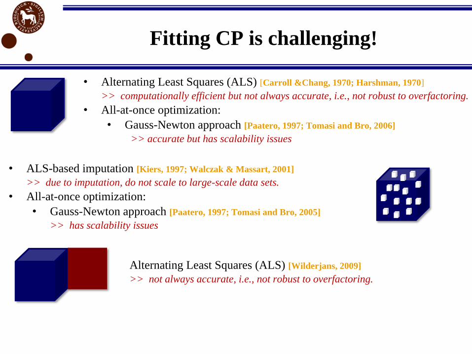
Fitting CP is challenging!
• Alternating Least Squares (ALS) [Carroll &Chang, 1970; Harshman, 1970]
>> computationally efficient but not always accurate, i.e., not robust to overfactoring.
• All-at-once optimization:
• Gauss-Newton approach [Paatero, 1997; Tomasi and Bro, 2006]
>> accurate but has scalability issues
• ALS-based imputation [Kiers, 1997; Walczak & Massart, 2001]
>> due to imputation, do not scale to large-scale data sets.
• All-at-once optimization:
• Gauss-Newton approach [Paatero, 1997; Tomasi and Bro, 2005]
>> has scalability issues
Alternating Least Squares (ALS) [Wilderjans, 2009]
>> not always accurate, i.e., not robust to overfactoring.
GOAL: Scalable and accurate algorithms for fitting a CANDECOMP/PARAFAC model
Proposed Approach: Gradient-based optimization
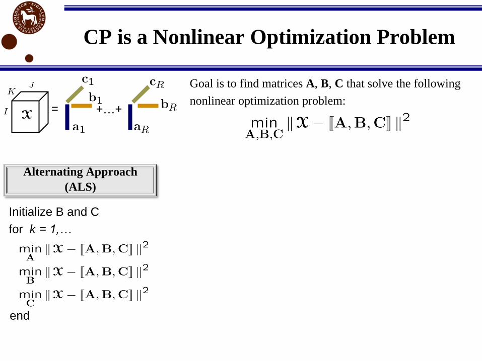
CP is a Nonlinear Optimization Problem
Goal is to find matrices A, B, C that solve the following
nonlinear optimization problem:
Alternating Approach
(ALS)
Initialize B and C
for k = 1,…
end
+…+=
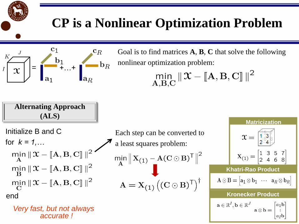
CP is a Nonlinear Optimization Problem
Goal is to find matrices A, B, C that solve the following
nonlinear optimization problem:
Optimization Problem
Alternating Approach
(ALS)
Initialize B and C
for k = 1,…
end
Very fast, but not always accurate !
Each step can be converted to
a least squares problem:
+…+=
Khatri-Rao Product
Matricization
Kronecker Product

CP is a Nonlinear Optimization Problem
Goal is to find matrices A, B, C that solve the following
nonlinear optimization problem:
Optimization Problem
Alternating Approach
(ALS)
Initialize B and C
for k = 1,…
end
All-at-once
Optimization
2nd order optimization
• Paatero, 1997;
Tomasi & Bro, 2006
• Gauss-Newton is used to solve
the nonlinear least squares
problem.
• Jacobian is IJK by (I+J+K)R
1st order optimization
• Paatero, 1999;
Acar, Dunlavy and Kolda, 2011
• Nonlinear CG
+…+=
Not scalable!Very fast, but not always
accurate !
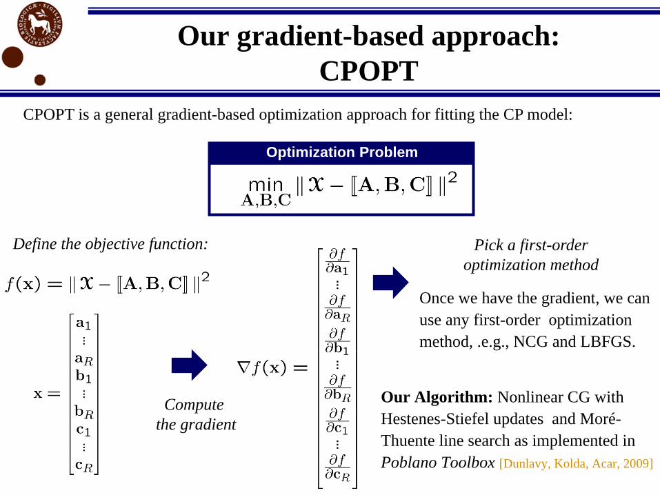
Our gradient-based approach:
CPOPT
CPOPT is a general gradient-based optimization approach for fitting the CP model:
Define the objective function:
Our Algorithm: Nonlinear CG with
Hestenes-Stiefel updates and Moré-
Thuente line search as implemented in
Poblano Toolbox [Dunlavy, Kolda, Acar, 2009]
Optimization Problem
Compute
the gradient
Once we have the gradient, we can
use any first-order optimization
method, .e.g., NCG and LBFGS.
Pick a first-order
optimization method

Gradient in Matrix Form
+…+=
Gradient
Note the relation with ALS:
Objective Function
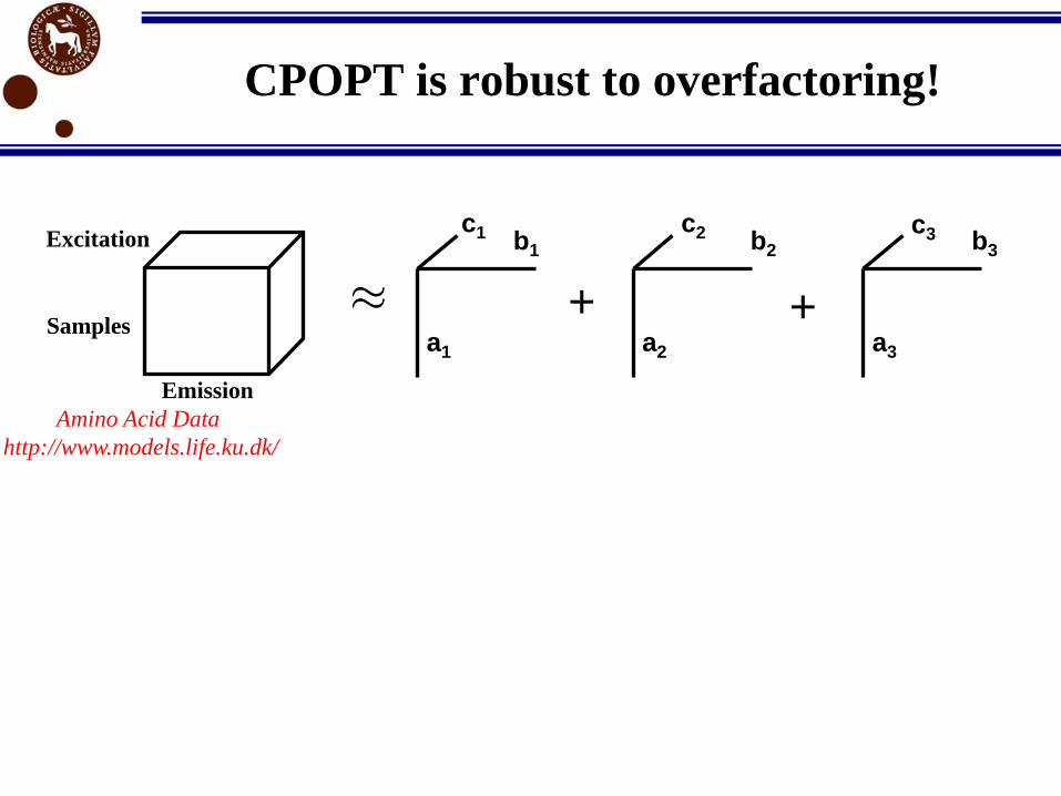
CPOPT is robust to overfactoring!
Samples
Emission
Excitation
+a1
b1
c1
+a2
b2
c2
a3
b3
c3
Amino Acid Data
http://www.models.life.ku.dk/
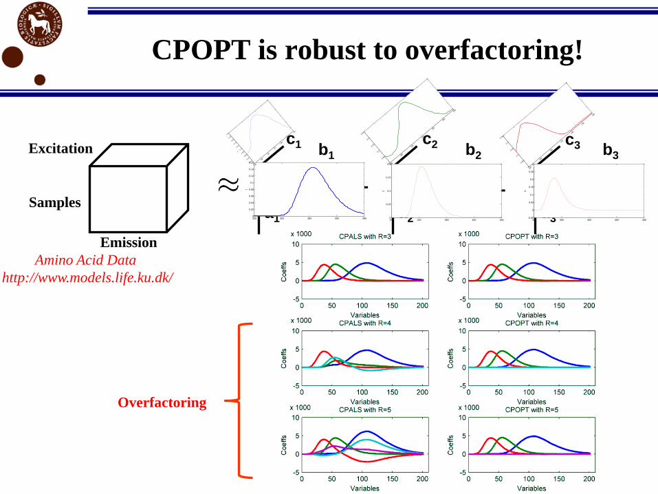
CPOPT is robust to overfactoring!
Emission
Excitation
+a1
b1
c1
+a2
b2
c2
a3
b3
c3
250 300 350 400 4500
0.02
0.04
0.06
0.08
0.1
0.12
0.14
0.16
1
240
250
260
270
280
290
300
00.
020.
040.
060.
08
0.1
0.12
0.14
0.16
0.18
0.2
1
250 300 350 400 4500
0.05
0.1
0.15
0.2
2
240
250
260
270
280
290
300
0
0.05
0.1
0.15
0.2
0.25
250 300 350 400 450-0.05
0
0.05
0.1
0.15
0.2
0.25
0.3
3
240
250
260
270
280
290
300
0
0.05
0.1
0.15
0.2
0.25
Overfactoring
Amino Acid Data
http://www.models.life.ku.dk/
Samples

CPOPT is computationally efficient!
Tensor Size:
50 x 50 x 50
Tensor Size:
250 x 250 x 250
Computational time for fitting an
R-component CP model :
Computational Cost (per iteration)
of fitting an R-component CP
model to a K x K x K tensorO(RK3) O(R3K3) O(RK3)

In the presence of missing data…
Given tensor and R (# of components), find matrices A, B, C that solve the following problem:
where the vector x comprises the entries of A, B, and C stacked column-wise:
Optimization Problem
+…+=I
JK
variables
Objective Function
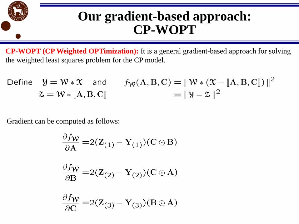
Our gradient-based approach:CP-WOPT
Gradient can be computed as follows:
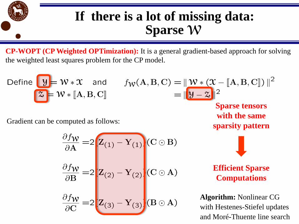
CP-WOPT (CP Weighted OPTimization): It is a general gradient-based approach for solving
the weighted least squares problem for the CP model.
If there is a lot of missing data: Sparse
Gradient can be computed as follows:
CP-WOPT (CP Weighted OPTimization): It is a general gradient-based approach for solving
the weighted least squares problem for the CP model.
Sparse tensors
with the same
sparsity pattern
Efficient Sparse
Computations
Algorithm: Nonlinear CG
with Hestenes-Stiefel updates
and Moré-Thuente line search

Step 1: Initialize matrices A, B, and C
Step 2: Complete the missing entries of X using the current model
Step 3: Compute A, B and C via alternating least squares, i.e.,
Step 4: Go back to Step 2 until convergence
Details on Alternative Techniques
ALS-based Imputation (EM-ALS):
NLS approach extended to missing data:
• Developed by Paatero, 1997 and Tomasi and Bro, 2005. We use INDAFAC by
Tomasi and Bro.
• Fits the model only to the known data entries just like CP-WOPT
• Uses Gauss-Newton
• Jacobian is (1-M)IJK by (I+J+K)R, where M is the missing data rate.
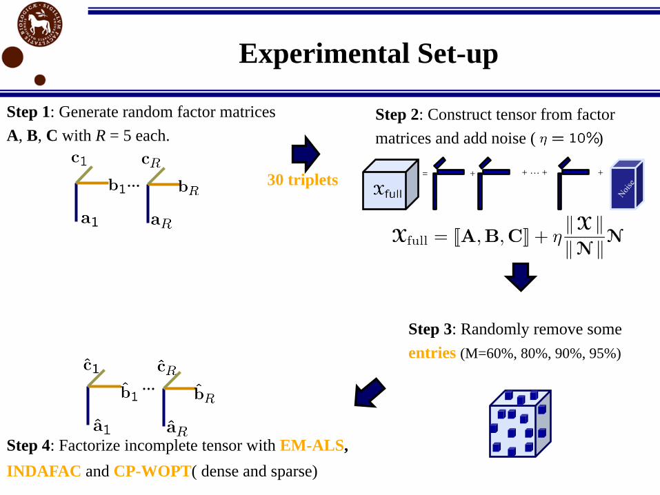
Experimental Set-up
Step 4: Factorize incomplete tensor with EM-ALS,
INDAFAC and CP-WOPT( dense and sparse)
Step 1: Generate random factor matrices
A, B, C with R = 5 each.
…
…
Step 3: Randomly remove some
entries (M=60%, 80%, 90%, 95%)
Step 2: Construct tensor from factor
matrices and add noise ( )
= + + + +30 triplets
Compute factor match score (FMS):
Best
FMS is 1!

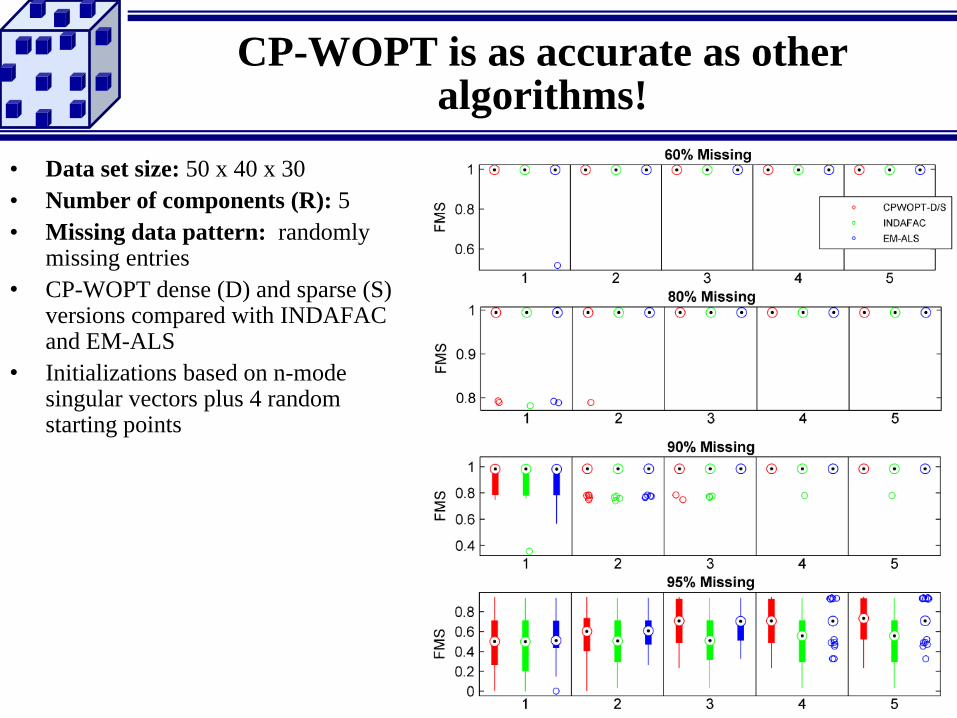
CP-WOPT is as accurate as other algorithms!
• Data set size: 50 x 40 x 30
• Number of components (R): 5
• Missing data pattern: randomly missing entries
• CP-WOPT dense (D) and sparse (S) versions compared with INDAFAC and EM-ALS
• Initializations based on n-mode singular vectors plus 4 random starting points
initialization
using
n-mode
singular vectors
random
init
random
init
random
init
random
init
CP-WOPT is as accurate as other algorithms!
• Data set size: 50 x 40 x 30
• Number of components (R): 5
• Missing data pattern: randomly missing entries
• CP-WOPT dense (D) and sparse (S) versions compared with INDAFAC and EM-ALS
• Initializations based on n-mode singular vectors plus 4 random starting points

• Data set size: 100 x 80 x 60
• Number of components (R): 5
• Missing data pattern: randomly
missing entries
• Smaller values of ratio indicate
more difficult problems:
Larger problems are easier!
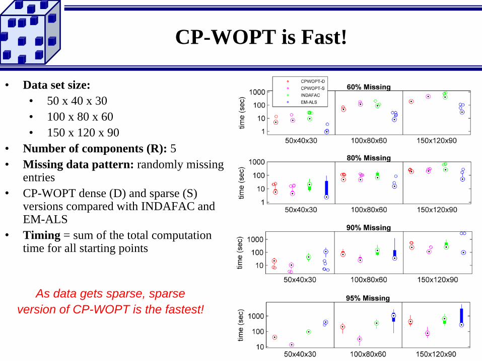
CP-WOPT is Fast!
• Data set size:
• 50 x 40 x 30
• 100 x 80 x 60
• 150 x 120 x 90
• Number of components (R): 5
• Missing data pattern: randomly missing entries
• CP-WOPT dense (D) and sparse (S) versions compared with INDAFAC and EM-ALS
• Timing = sum of the total computation time for all starting points
As data gets sparse, sparse
version of CP-WOPT is the fastest!
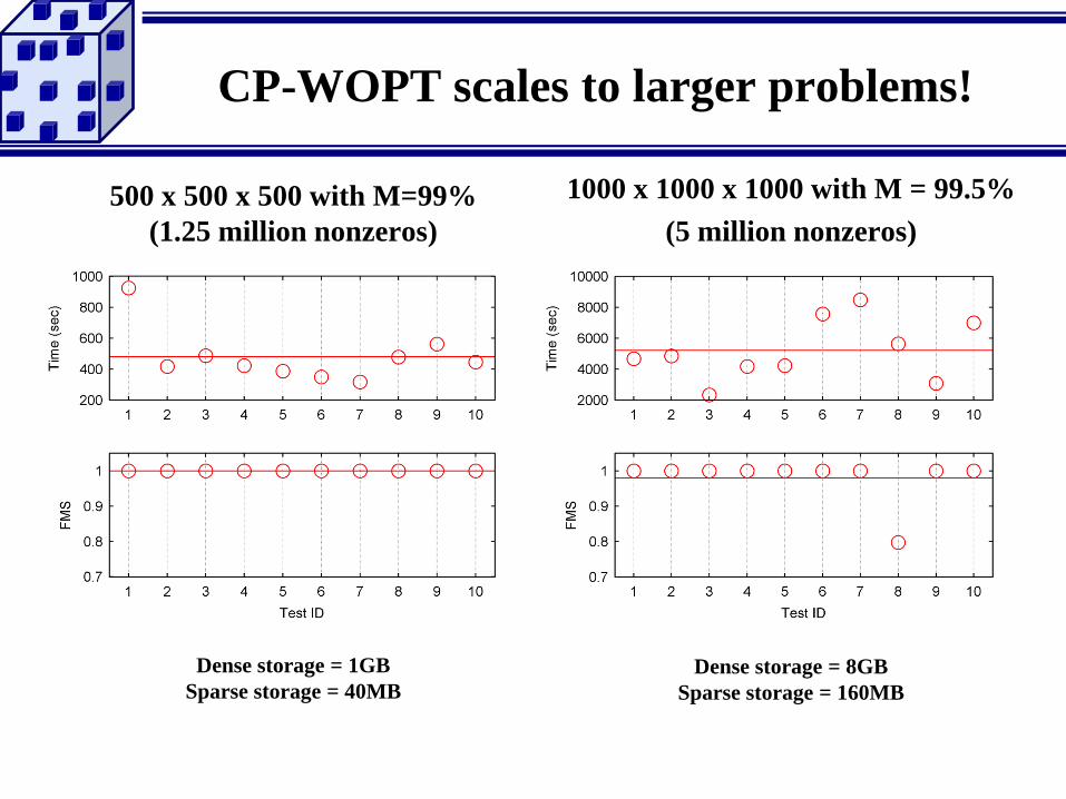
CP-WOPT scales to larger problems!
500 x 500 x 500 with M=99%
(1.25 million nonzeros)
1000 x 1000 x 1000 with M = 99.5%
(5 million nonzeros)
Dense storage = 1GB
Sparse storage = 40MB
Dense storage = 8GB
Sparse storage = 160MB
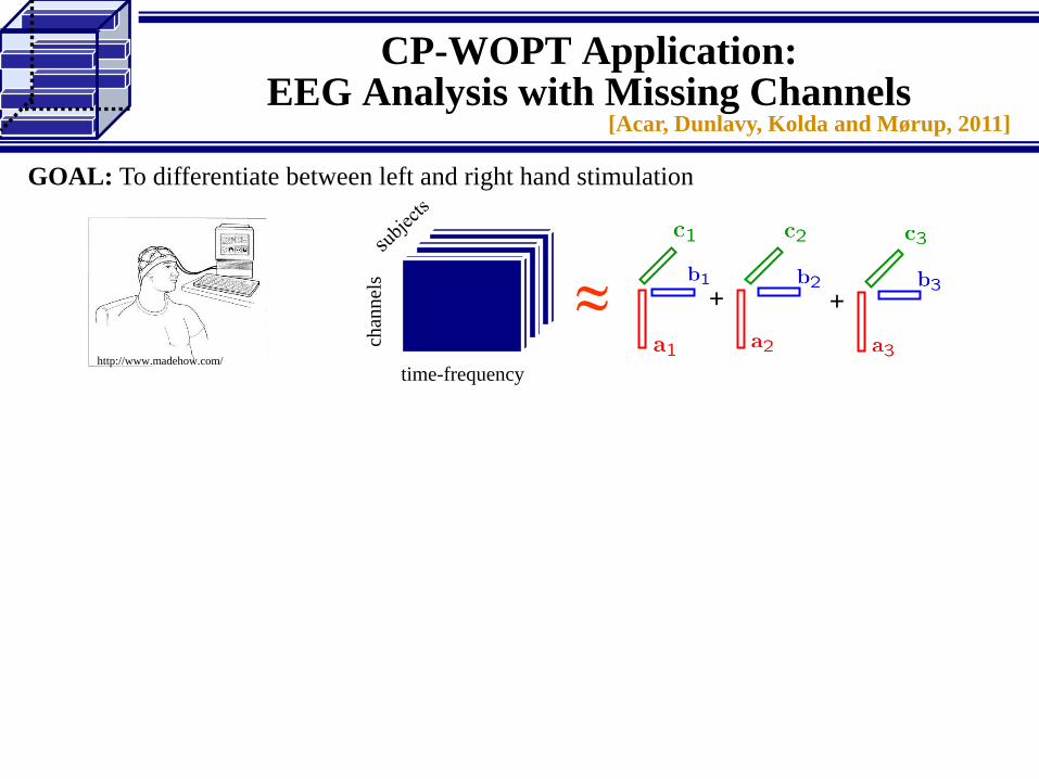
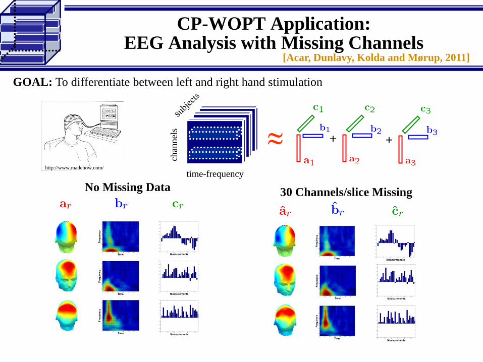
CP-WOPT Application:EEG Analysis with Missing Channels
GOAL: To differentiate between left and right hand stimulation
chan
nel
stime-frequency
≈ + +
http://www.madehow.com/
[Acar, Dunlavy, Kolda and Mørup, 2011]
GOAL: To differentiate between left and right hand stimulation
chan
nel
stime-frequency
≈ + +
No Missing Data 30 Channels/slice Missing
http://www.madehow.com/
CP-WOPT Application:EEG Analysis with Missing Channels
[Acar, Dunlavy, Kolda and Mørup, 2011]
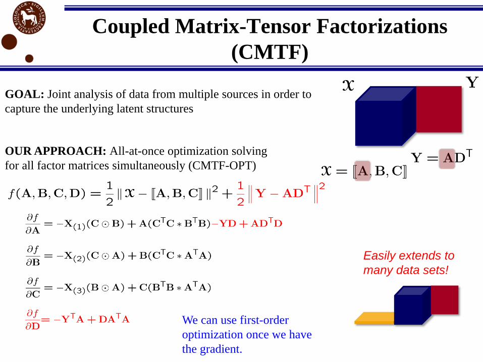
Coupled Matrix-Tensor Factorizations
(CMTF)
GOAL: Joint analysis of data from multiple sources in order to
capture the underlying latent structures
We can use first-order
optimization once we have
the gradient.
OUR APPROACH: All-at-once optimization solving
for all factor matrices simultaneously (CMTF-OPT)
Easily extends to
many data sets!

CMTF is also useful for
missing data recovery
In many applications such as recommendation systems, the goal
is to recover missing entries.
Modeling
only
Modeling both
and
CMTF can deal with larger
amounts of missing data!
Tensor Completion Score (TCS)

Experimental Set-up
Generate factor
matrices
Solve f using CMTF-ALS
and CMTF-OPT+ … + =
…+ + =
Construct tensor and matrix Y and
add noise
Data Generation:
Accuracy as the performance metric : The algorithm is accurate if original factors, i.e., A, B, C
and D, match with the extracted factors, i.e., .
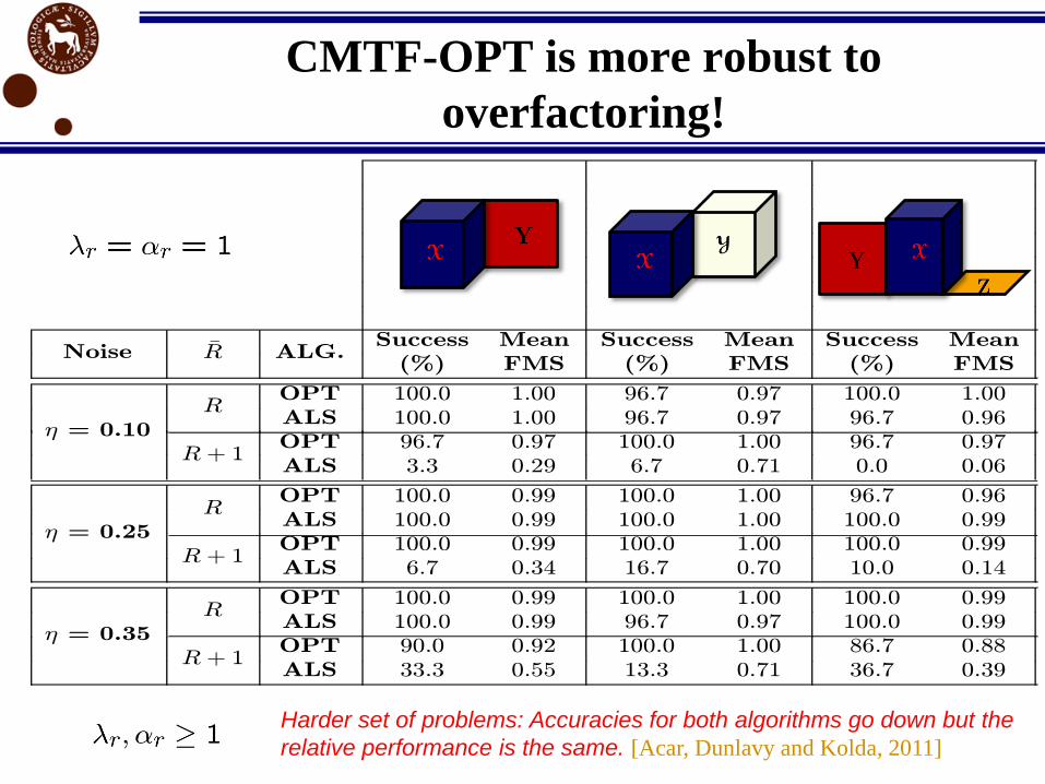
Noise ¹R ALG.Success Mean Success Mean Success Mean
(%) FMS (%) FMS (%) FMS
´ = 0.10
ROPT 100.0 1.00 96.7 0.97 100.0 1.00
ALS 100.0 1.00 96.7 0.97 96.7 0.96
R + 1OPT 96.7 0.97 100.0 1.00 96.7 0.97
ALS 3.3 0.29 6.7 0.71 0.0 0.06
´ = 0.25
ROPT 100.0 0.99 100.0 1.00 96.7 0.96
ALS 100.0 0.99 100.0 1.00 100.0 0.99
R + 1OPT 100.0 0.99 100.0 1.00 100.0 0.99
ALS 6.7 0.34 16.7 0.70 10.0 0.14
´ = 0.35
ROPT 100.0 0.99 100.0 1.00 100.0 0.99
ALS 100.0 0.99 96.7 0.97 100.0 0.99
R + 1OPT 90.0 0.92 100.0 1.00 86.7 0.88
ALS 33.3 0.55 13.3 0.71 36.7 0.39
CMTF-OPT is more robust to
overfactoring!
Harder set of problems: Accuracies for both algorithms go down but the
relative performance is the same. [Acar, Dunlavy and Kolda, 2011]
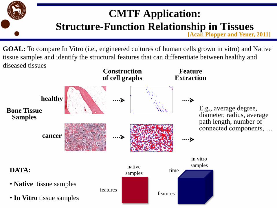
CMTF Application:
Structure-Function Relationship in Tissues[Acar, Plopper and Yener, 2011]
GOAL: To compare In Vitro (i.e., engineered cultures of human cells grown in vitro) and Native
tissue samples and identify the structural features that can differentiate between healthy and
diseased tissues
Bone Tissue Samples
healthy
cancer
Construction of cell graphs
Feature Extraction
E.g., average degree, diameter, radius, average path length, number of connected components, …
DATA:
• Native tissue samples
• In Vitro tissue samples
native
samples
features
in vitro
samples
features
time
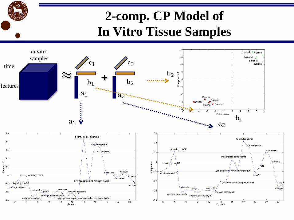
2-comp. CP Model of
In Vitro Tissue Samples
+features
time
in vitro
samples

Coupled Analysis of
Native and In Vitro Tissue Samples
feat
ure
s
time
Can
cer
Norm
al
Can
cer
Norm
al
in vitro
samples
native
samples
+
+
First component
differentiates between
cancer and normal!

Coupled Analysis of
Native and In Vitro Tissue Samples
feat
ure
s
time
Can
cer
Norm
al
Can
cer
Norm
al
in vitro
samples
native
samples
+
+
First component
differentiates between
cancer and normal!

Summary & Future Work
Challenge: Scalable and accurate algorithms for
– Fitting a CP model
– Fitting a CP model to incomplete data
– For coupled matrix and tensor factorizations
Our Approach: All-at-once optimization using gradient-based algorithms
– CPOPT/ CP-WOPT for fitting a CP model
• As accurate as alternative techniques
• Scales to larger data sets compared to alternative methods.
– CMTF-OPT for modeling coupled data sets
• Builds onto CPOPT/CP-WOPT and has the same nice properties
Future Work:– Coupled Factorizations:
• Constraints for better interpretability – sparsity and non-negativity
• Applications in biomedical informatics
+ …=

Thank you!
Evrim [email protected]
http://www.models.life.ku.dk/users/acare/
SURVEY
E. Acar and B. Yener, Unsupervised Multiway Data Analysis: A Literature Survey, IEEE Transactions on Knowledge
and Data Engineering, 21(1): 6-20, 2009.
ALGORITHMS
CMTF-OPT E. Acar, T.G. Kolda and D.M. Dunlavy, All-at-once Optimization for Coupled Matrix and Tensor
Factorizations, KDD Workshop Proceedings for the 9th Workshop on Mining and Learning with Graphs, 2011.
CP-OPT (code available with Tensor Toolbox v2.4) E. Acar, T.G. Kolda and D.M. Dunlavy, A Scalable Optimization
Approach for Fitting Canonical Tensor Decompositions, Journal of Chemometrics, 25(2): 67-86, 2011.
CP-WOPT (code available with Tensor Toolbox v2.4) E. Acar, D.M. Dunlavy, T.G. Kolda and M. Mørup, Scalable
Tensor Factorizations for Incomplete Data, Chemometrics and Intelligent Laboratory Systems, 106: 41-56, 2011.
Poblano Toolbox. D.M. Dunlavy, T.G. Kolda and E. Acar, Poblano v1.0: A Matlab Toolbox for Gradient-Based
Optimization, Sandia National Laboratories, Albuquerque, NM and Livermore, CA, Technical Report SAND2010-
1422, March 2010.
APPLICATIONS
Epilepsy. E. Acar, C.A. Bingöl , H. Bingöl, R. Bro and B. Yener, Multiway Analysis of Epilepsy Tensors,
Bioinformatics, 23(13):i10-i18, 2007.
Cell-Graphs. E.Acar, G. Plopper and B. Yener, Coupled Analysis of in Vitro and Histology Tissue Samples to
Quantify Structure- Function Relationship, Submitted for Publication, June 2011.