all in one · clustering’ of’ nodes’ in a’ network’ can be’ quantified with...
TRANSCRIPT
1
Title: Metabolic networks, structure and dynamics Name: Guilhem Chalancon1 , Kai Kruse1 and M Madan Babu1 Affil./Addr.: MRC Laboratory of Molecular Biology Hills Road, CB2 0QH, Cambridge,UK +44 (0) 1223 402208 (GC) guilhem@mrc-‐lmb.cam.ac.uk, (KK) kkruse@mrc-‐lmb.cam.ac.uk, (MMB) madanm@mrc-‐lmb.cam.ac.uk
Metabolic networks, structure and dynamics Synonyms none. Definition The metabolism encompasses the sum of all biochemical reactions catalysed by enzymes in a cell. Taken together, these reactions form interconnected metabolic pathways that shape a dynamical circuitry referred to as metabolic network (MN, see Fig.1). Here we describe the main methods relevant to the study of structural and dynamical understanding of the properties of metabolic networks (For an overview of metabolic network reconstruction, please refer to Metabolic Network reconstructions).
Characteristics Structural analysis of metabolic networks Knowledge about the topological properties of a metabolic network is central to the understanding of its function. Graph theoretic approaches have been extensively employed to derive global network features such as topological organization and robustness properties (Ravasz, 2003 and Palsson, 2006), determine the importance of individual enzymes or metabolites and curate the network by predicting missing components. Global network properties A number of graph theoretic measures describe the global structure of MNs (Discrete Models and Mathematics, Graph Theoretic Approaches). The degree distribution is the probability distribution of links per node (degree) in a network. In MNs it is highly non-‐random and can be fitted by a power law, reflecting a scale-‐free topology: A small number of metabolites act as hubs involved in a very large number of reactions (e.g. ATP, Coenzyme A), making the network extremely robust to random loss of nodes. Clustering of nodes in a network can be quantified with the global clustering coefficient (Clustering coefficient). It has been shown that MNs consist of a high number of strongly connected modules that are combined in a hierarchical manner, resulting in a high, size-‐independent clustering coefficient -‐ despite the networks scale-‐free properties. In addition to the clustering coefficient, the distribution of shortest paths between any two nodes in the network demonstrates the small world

2
properties of metabolic networks: Any metabolite in the network can be reached via a small number of edges. From the distribution two values can be derived: The characteristic path length (average over all shortest paths) and the network diameter (longest shortest path). Both values are typically very small in MNs. (Small-‐world Property of Networks) The degree assortativity coefficient reflects the tendency of nodes in a network to form links with nodes of similar degree. Its value is negative in MNs, indicating disassortative mixing of nodes: Nodes with a high degree preferentially connect to nodes of lower degree. Please also refer to Graph Algorithms in Network Analysis. Local network analysis In addition to local versions of the above measures, attempts have been made to examine the network on a local scale. Network motifs, defined as sub-‐networks that occur significantly more often in a network than expected by chance, have been identified and shown to perform specific tasks in MNs (Alon, 2007). Among them are futile cycles that dissipate energy in the MN, switches directing the metabolite flux and feed-‐forward motifs that provide regulatory control (see also Network motifs, Feed-‐forward loops and Fig. 2). Overall, it appears that the recurrence of such local architecture enables biological adaptation to varying environments (Wenzhe et al., 2009). The number of shared neighbors between two nodes is called a topological overlap. By calculating it for every node and subsequent clustering (Clustering), a topological overlap map can be generated. Metabolites with similar biochemical properties cluster together, demonstrating functional organization of sub-‐networks in MNs. Also see Modules in networks: algorithms and methods.
From static to dynamic models Despite their usefulness, graph-‐based approaches do not depict the dynamical behavior of metabolic networks. However, stoichiometry based approaches and kinetic models permit to investigate the fluxes of metabolites within metabolic pathways, which is of great interest with respect to functional analysis of metabolism and pharmacological studies. Exclusively stoichiometry based On the most basic level, analysis of MN dynamics operate on stoichiometry of reactions alone, without integrating additional information, such as enzymatic rates or thermodynamic constraints. Boolean network analysis (BNA) use Boolean logic to infer the capacity to produce given metabolites and the activities of given reactions, by treating each node as a switch that can either be on or off. After setting appropriate starting states, in which certain reactions are switched off, the state of all other nodes is determined by iteratively applying Boolean rules, until no further change occurs. BNA has been applied successfully in model curation and network robustness analysis (Boolean Network, Robustness). Network expansion is a method closely related to BNA: Starting with a seed of nutrients, the so-‐called scope (all producible metabolites and active reactions) is determined iteratively, based on Boolean state switches. Thus, the biosynthetic capacities of a MN can be assessed. Petri nets are directed bipartite graphs that are capable of modelling a discrete flow of mass within a MN. They are supported by a well-‐developed mathematical theory that even allows a transition to continuous simulations (Cell Cycle Modelling, Petri nets).

3
Chemical reaction network theory (CRNT) and species-‐reaction graphs (SR graphs) use topology and a few basic assumptions to derive the stability (Stability) and the possibility of multistability (Bistability) of a MN. However, due to their computational complexity, they are unsuitable at present for genome-‐scale models. Integrating additional information Generally, metabolic network dynamics are dependent on a multitude of factors in addition to network structure, e.g. reaction thermodynamics, kinetics and rates or environmental conditions. More complex approaches are able to integrate this information (Steuer, 2007). Flux balance analysis (FBA) calculates optimal reaction rates at steady state in the network (flux distribution) by formulating a linear optimization problem. Reaction rates are constrained by the network stoichiometry, metabolite availability and thermodynamic properties of the catalysing enzymes. Typically, the optimization goal is maximization of biomass, equivalent to growth, but other objective functions such as maintenance of energy balance have been used. FBA is especially useful for simulating network disturbances, such as enzyme loss or nutrient shortage (Ruppin et al., 2010). (Linear programming, Stable steady state, Flux Balance Analysis) Time dynamics modelling is a mathematical modelling technique that uses a system of differential equations to perform detailed simulations of the metabolic concentration dynamics -‐ the use of partial differential equations moreover permits to integrate spatial information. It relies on explicit reaction kinetics, including enzymatic parameters relative to the equilibrium constraints and maximal reaction rates. Because this information remains unavailable for many enzymes and is dependent on physical parameters, cycles of parameter estimation and optimization are generally required. As a result, differential equation modelling becomes increasingly difficult as the network size grows and is practically infeasible for networks as large as metabolic networks. However, time dynamics modelling is an extremely valuable tool for analysing and predicting the behaviour of individual pathways or of reduced models of metabolic networks (Dynamical Systems Theory, Ordinary Differential Equations, Stability Analysis, ODE model). Structural kinetic modelling (SKM) is another mathematical modelling technique that attempts to compensate for the lack of explicit kinetics by statistically exploring the entire parameter space at a predefined steady state of the system. It is thus possible to describe the possible dynamics of the system and to identify key metabolites and enzymes within the MN. Based on thermodynamic constraints and the stoichiometric structure of the network’s elementary modes (EMs), extreme pathways (EPs) and minimal metabolic behaviors (MMBs) are decompositions of the metabolic network into unique sets of functionally meaningful pathways. They allow a detailed analysis of metabolic pathways and have notably been applied to investigate the structure, robustness and regulation of microbial metabolic networks.
4
Conclusion The reconstruction of metabolic networks at a genomic scale has been greatly facilitated by the development of sequencing technologies and high throughput “omics” methods. A large number of sophisticated approaches permits the analysis of the structure and dynamics of large sets of biochemical reactions. Graph theoretical measures show that MNs possess a unique set of structural characteristics: They are scale-‐free, yet display a highly modular, hierarchical architecture and are small-‐world networks that show a disassortative associations of their nodes. On a local level, network motifs emphasize that the structural organization in feedback loops and in multiple-‐input motifs can influence the dynamics and the regulation of metabolic pathways. Network dynamics can be modelled by approaches with a wide range of complexity, depending on the features of interest: If the network is sufficiently small and explicit kinetics are available, a modelling with differential equations is possible providing detailed metabolite concentration dynamics. Larger networks dynamics can be accessed by FBA or SKM, which does not rely on kinetic parameters, but in turn do not provide as much detail. In the case where only stoichiometric information is available, more basic approaches such as BNA, network expansion or Petri nets can be used.
References 1. Uri Alon. Network motifs: theory and experimental approaches. Nat Rev Genet, 8(6):450–461, Jun
2007.
2. Adam M Feist, Markus J Herrgrd, Ines Thiele, Jennie L Reed, and Bernhard Palsson. Reconstruction of
biochemical networks in microorganisms. Nat Rev Microbiol, 7(2):129–143, Feb 2009.
3. Bernhard O. Palsson. Systems biology: properties of reconstructed networks. Cambridge University
Press, 1st edition, January 2006.
4. Erzsbet Ravasz and Albert-‐Loszlo Barabasi. Hierarchical organization in complex networks. Phys Rev E
Stat Nonlin Soft Matter Phys, 67(2 Pt 2):026112, Feb 2003.
5. Eytan Ruppin, Jason A Papin, Luis F de Figueiredo, and Stefan Schuster. Metabolic reconstruction,
constraint-‐based analysis and game theory to probe genome-‐scale metabolic networks. Curr Opin
Biotechnol, 21(4):502–510, Aug 2010.
6. Ralf Steuer. Computational approaches to the topology, stability and dynamics of metabolic networks.
Phytochemistry, 68(16-‐18):2139–2151, 2007.
7. Wenzhe Ma, Ala Trusina, Hana El-‐Samad, Wendell A Lim, and Chao Tang. Defining network
topologies that can achieve biochemical adaptation. Cell, 138(4):760–773, Aug 2009.
5
Cross-‐references Metabolic Network Reconstructions (new) Discrete Models and Mathematics, Graph Theoretic Approaches (0000) Clustering coefficient (new) Small-‐world Property of Networks (0002) Graph Algorithms in Network Analysis (0003) Network Motifs (0461) possibly redundant with Network Topology Motif (0562) Feed forward loops (0463) Clustering (00511) Modules in networks: algorithms and methods (0557) Boolean Network (0442) Robustness (0538) Cell Cycle Modelling, Petri nets (00027) Stability (0494) Bistability (0526) Linear programming (0406) Stable steady state (0495) Flux Balance Analysis (new) Dynamical Systems Theory, Ordinary Differential Equations (0000) Dynamical Systems Theory, Stability analysis (0000) ODE model (0381)

6
Figures and Tables
Fig. 1. Metabolic networks are multipartite directed graphs, comprising a set of genes which codes (dark blue) for a set of enzymes (blue), whose biochemical reactions constitute a third set (green) to which compounds are connected (red) to represent metabolic reactions. An example of metabolic pathway is given by a simplified version of the glycolytic pathway in Human. The metabolic pathway can be collapsed into two types of graph: a reaction graph, in which each node represents a reaction (here labelled by the EC number of the corresponding enzyme), and links connect products of one reaction to reactants of the other; a substrate graph, in which compounds are connected to each other by links that represent metabolic reactions.

7
Fig. 2. The structure of metabolic networks can be studied at global, intermediate and local scales, reflecting distinct organizational properties. The metabolic network -‐ represented here in a circle-‐layout contains sets of interrelated metabolic pathways, which themselves contain frequent network motifs. Futile-‐cycle and single-‐input-‐motifs are highlighted in the metabolic pathway of the pyrimidine metabolism of E.coli (KEGG: ec00240). Distinct properties of metabolic networks such as scale-‐freeness and modularity can be investigated at the global architecture or at a more local level, respectively. As a consequence of complexity and lack of annotations to determine parameters, explicit models are constrained to a local scale, while the modelling of entire metabolic networks is mostly achieved by the use of topology and stoichiometry based approaches.
8
Title: Metabolic networks and their applications Name: Guilhem Chalancon1 , Kai Kruse1 M Madan Babu1 Affil./Addr.: MRC Laboratory of Molecular Biology Hills Road, CB2 0QH, Cambridge,UK +44 (0) 1223 402208 (GC) guilhem@mrc-‐lmb.cam.ac.uk, (KK) kkruse@mrc-‐lmb.cam.ac.uk, (MMB) madanm@mrc-‐lmb.cam.ac.uk
Metabolic networks and their applications Definition The reconstruction of genome-‐scale models of metabolic networks (See Metabolic Network reconstructions) has permitted us to form an accurate picture of the metabolic pathways of numerous organisms. Applications of metabolic network analyses, which allow us to analyse problems ranging from single pathway to multi-‐species studies, are reviewed in this article. Table 1 summarizes established methodologies and software relevant to these applications.
Characteristics Knowledge gap-‐filling: discovery of missing pathways The systematic characterization of gene functions at a genomic scale remains challenging. For instance, up to 13% of gene functions in the intensively studied bacterium Escherichia coli remain currently unknown. Many of these genes have possible roles in the metabolic network. Errors in the topological consistency of metabolic networks can be used to fill some of the encountered gaps. These errors might include, for example, pathway dead-‐ends, which corresponds to the endless accumulation of metabolites, or ‘unconnected’ metabolites; both indicating that some reactions are missing from the annotations (Fig. 1A). The comparison between experiments and computational reconstructions of metabolic networks provides a good framework to identify missing reactions and characterize the function of unknown ORFs. Comparisons can, for example, be based on network-‐topology and mRNA co-‐expression data (Feist and Palsson, 2009). Alternatively, optimization-‐based procedures (see Flux Balance Analysis) can be used to infer possible gains in fitness for a given organism when adding news reactions from databases to the metabolic network (Metabolic Network Reconstructions). Thus, potential gaps in reconstruction can be uncovered by energetic considerations of metabolic pathways. Contextualization of high throughput data in metabolic networks Abstractly, metabolic networks represent all known possible roads that connect cellular compounds to each other via biochemical transformations. This static map can be contextualized by taking into account expression levels or the phenotypic features of its enzymes in a given condition. The mapping of high-‐

9
throughput expression data onto metabolic networks permits to indicate the state of usage of known metabolic pathways (Oberhardt et al., 2009). Generally, a contextualization consists of constraining in silico metabolic fluxes to match experimental data. Such data might be condition-‐specific mRNA expression levels based on microarray or RNA sequencing, or protein expression levels (Fig. 1B). It is also possible to investigate how phenotypic data or essential genes interrelate with the network topology. Study of diseases through metabolic Systems Biology approach An increasing number of diseases are now seen as the result of drastic perturbations of cellular functions that involve large sets of genes, whose interrelations are intricate. In particular, diseases such as cancer or diabetes cause large perturbations in cellular metabolism. Hence, the study of metabolic networks -‐ particularly of the perturbation of interactions and fluxes -‐ can facilitate a better understanding of the physio-‐pathology of such diseases. It notably allows for an understanding of how and why a change in activity or expression levels of a few enzymes can propagate considerable perturbations into entire cellular functions. Anomalies in topology or metabolic fluxes of metabolic networks can be measured or simulated to retrieve genes involved in the pathology and potential drug-‐targets (Fig. 1C). In practice, metabolic networks are often combined with gene-‐regulatory networks and protein-‐protein interaction networks. The human gene-‐regulatory and metabolic networks, for example, have successfully been used to identify transcription factors and metabolites that could be used for clinical diagnostics of type 2 diabetes (del Sol et al., 2010). Metabolic engineering Existing metabolic networks can be altered to optimize specific cellular functions which might be either pre-‐existing or newly designed. This type of ‘engineering’ is made -‐ at the molecular level -‐ by the introduction of mutations, deletions, insertions and up or down-‐regulations of enzymes of interest (Fig. 1D). Because efficient designs are often non-‐intuitive, predicting the right adjustments of metabolic fluxes necessary to reach the defined objective necessitates computational strategies based on constraint-‐methods. Metabolic engineering generally focuses on the production of high levels of metabolites of medical or industrial interest. They are so far mostly performed in bacteria or yeast. Typical examples of engineered strains produced in the industry are ethanol-‐, lactic acid or lycopene-‐producing microorganisms. Human steroid hormones such as hydroxycortisone can also be synthesized in yeast. A future field of application will likely be the area of synthetic biology, which has gained increased interest with the recent completion and incorporation of the first synthetic bacterial genome. Reduction of experimental time and effort Ideally, metabolic network modelling and experimental analysis form an iterative cycle in which the results of one can be utilized to improve the other (Fig. 1E). As detailed in the previous sections, experimental results can be used to change the behavior of the metabolic network analysis. In turn, results from the computational analysis can assist in adjusting the experimental setup, allowing

10
scientists to focus on particular aspects of a problem. This approach can drastically reduce the experimental effort by prioritizing the validation of computationally predicted hypothesis about the system under investigation instead of focusing on potentially less informative aspects of a problem (Oberhardt M. et al. 2009). Multi-‐species investigations The integration of comparative genomics with metabolic network information has lead to many promising outcomes. (i) In evolutionary sciences, it allows to relate metabolism to phenotypic diversity among closely-‐related species and their short-‐term evolution. Although this area of applications remains relatively unexplored in comparison with the other applications of metabolic networks, promising insights have shown that E.coli strains adapt to the medium they grow in with characteristics close to their the optima predicted by flux balance analysis (Flux Balance Analysis, Oberhardt et al. 2009). (ii) In metagenomics, it permits the study of interactions of multiple organisms in the same environment. Comparative analysis of metabolic networks (Fig. 1F) provides information about the adaptive evolution of microorganisms, the consequences of horizontal gene transfers and the evolution of minimal metabolic networks in parasites (Pal et al. 2006).
Conclusion The study of metabolic networks with regard to their topological structure has uncovered the existence of regulatory motifs and system-‐wide properties leading to a better understanding of cellular metabolism (Metabolic network, structure and dynamics). This has also lead to applications that range from the contextualization of high throughput data to the in silico discovery of new metabolic pathways. Metabolic network reconstructions also guide metabolic engineering and improve our understanding of multiple-‐species interactions.
Cross-‐references 1. Mass action stochastic analysis 2. KEGG (00472) 3. Metabolic Network and their evolution (0004) 4. Modularity (00475) 5. Multi-‐Ouput FFLs (00555) 6. Network Alignments (0482) 7. Network Motifs (0461) possibly redundant with Network Topology Motif (0562) 8. Pathway (0467) 9. Robustness (0538) 10. Stable Steady State (0495) 11. Feed forward loops (0463)

11
References 1. Antonio del Sol, Rudi Balling, Lee Hood, and David Galas. Diseases as network perturbations.
Curr Opin Biotechnol, 21(4):566–571, Aug 2010.
2. Adam M Feist and Bernhard Palsson. The growing scope of applications of genome-‐scale metabolic
reconstructions using escherichia coli. Nat Biotechnol, 26(6):659–667, Jun 2008.
3. Hongwu Ma and Igor Goryanin. Human metabolic network reconstruction and its impact on drug
discovery and development. Drug Discov Today, 13(9-‐10):402–408, May 2008.
4. Matthew A Oberhardt, Bernhard Palsson, and Jason A Papin. Applications of genome-‐scale
metabolic reconstructions. Mol Syst Biol, 5:320, 2009.
5. Bernhard O. Palsson. Systems biology: properties of reconstructed networks. Cambridge University
Press, 1st edition, January 2006.
6. Gregory Stephanopoulos, Hal Alper, and Joel Moxley. Exploiting biological complexity for strain improvement through systems biology. Nat Biotechnol, 22(10):1261–1267, Oct 2004. 7. Pal, C. et al. Chance and necessity in the evolution of minimal metabolic networks. Nature 440, 667–670 2006 8. Maxime Durot, Pierre-‐Yves Bourguignon & Vincent Schachter. Genome-‐scale models of bacterial metabolism: reconstruction and applications. FEMS Microbiol Rev 33 (2009) 164-‐190
Network property discovery
Flux sampling: sampling of flux distributions among all possible metabolic states.
Flux coupling: detection of pairs of reactions whose fluxes are coupled
Elementary modes and extreme pathways:
Contextualization of high throughput data
Metabolic Adjustment by Differential Expression (MADE). Significant changes in gene expression integrated into metabolic models
http://bme.virginia.edu/csbl/downloads.php
Metabolic engineering: adjustments and production predictions
MOMA: prediction of flux distributions under gene deletions. The algorithm minimizes the overall changes in flux as compared to wild type.
http://openwetware.org/wiki/MoMA

12
ROOM (Regulatory On/Off minimization): prediction of growth (biomass) under gene deletions.
OptStrain: prediction of reaction to add to enhance the production of the metabolite of interest
RobustKnock: predicts gene deletion strategies taking into account the presence of competing pathways in the network.
http://www.cs.technion.ac.il/∼tomersh/tools/
OptFlux: metabolic engineering workbench http://www.optflux.org/
Table 1: Analytical methods and softwares for metabolic network applications.
Figure 1: Applications of metabolic networks. Gray shading indicates cell boundaries, circles represent metabolites, arrows within and across cell boundary correspond to reactions. Panel A: Detection and correction of unconnected metabolites (a) and dead ends (b). Panel B: Mapping expression data, kinetic and concentration measurements onto the metabolic network; size of circles represents concentration change, size and depiction of arrows indicates reaction flux change. Panel C: Genetic disease (SNP mutation causing change in expression) alters network simulation behaviour. Panel D: Directed introduction of genes can change network topology. Panel E: Iterative cycle of experiments and network analysis. Panel F: Comparison of metabolic networks of two species

13
Title: Metabolic network reconstruction Name: Guilhem Chalancon1 , Kai Kruse1 and M Madan Babu1 Affil./Addr.: MRC Laboratory of Molecular Biology Hills Road, CB2 0QH, Cambridge,UK +44 (0) 1223 402208 (GC) guilhem@mrc-‐lmb.cam.ac.uk, (KK) kkruse@mrc-‐lmb.cam.ac.uk, (MMB) madanm@mrc-‐lmb.cam.ac.uk
Metabolic network reconstructions Synonyms none. Definition The metabolism encompasses the sum of all biochemical reactions catalyzed by enzymes in a cell. Taken together, these reactions form interconnected metabolic pathways that shape a dynamical circuitry referred to as metabolic network (MN). Recent progress in genome annotations and the advancement of omics have made the extraction of metabolism-‐related information possible at a genomic scale. This has launched large efforts in network reconstruction and predictive model building. These include reconstructions for organisms with limited biochemical data, whose network can be reconstructed relying on genome annotations only (Feist et al., 2009). Formalism of metabolic networks Metabolic networks (MN) consist of bipartite graphs that include a set of metabolites and a set of enzymes -‐ linked together by arcs that represent biochemical associations and dissociations (See also Metabolic Networks, Structure and Dynamics). Metabolic network reconstruction Genome annotations are used in a series of semi-‐automated steps to reconstruct a model of a metabolic network. In an ideal case, the following information should be included into the model: 1. The list of all potential enzymes present in the organism of interest 2. The substrates and products of enzymatic reactions 3. The stoichiometric coefficients of each of these compounds 4. Information about thermodynamic reversibility or irreversibility of each reaction 5. Conditions for the activity or inactivity of each enzyme 6. Subcellular localizations of each enzyme

14
Methodological approach The process of constructing a metabolic networks is depicted in Figure 1. In general, genome databases, such as KEGG, MetaCyc or the SGD (see Table 1 for a complete list), are used to extract unique identifiers of putative enzymes and metabolites. This allows the use of automated tools which mine the available data (Table 1), supplemented by existing literature, to determine all possible reactions catalysed by this set of enzymes. These usually link Enzyme Commission numbers (EC) to reactions that have been characterized biochemically in other organisms, with the assumption that conserved enzymes between the reference organism and the target organism carry out identical reactions. The EC nomenclature database, called ENZYME can be found on the ExPASy website (Table 1). However, such an automated extraction does not account for substrate specificity and enzyme activity, which can drastically vary across orthologous enzymes. Additionally, the available information is often incomplete; specific enzyme properties or even entire reactions might be missing from the annotations. Therefore, a manual curation of the network constitutes the second step of MN reconstruction. Possible considerations for model consistency are reaction thermodynamics and activity, producibility of metabolites (network ‘dead ends’) and chemical mass balance of equations. The individual metabolic reactions are then connected in a network model. The final step of the reconstruction consists of the integration of meta-‐data into the MN. This includes high-‐throughput data describing expression levels and genetic interactions, as well as flux and metabolite concentration measurements (Palsson, 2006; Ruppin et al. 2010). This process is described in more details in Metabolic networks and their applications. Available models Network reconstructions have nowadays been assembled for organisms from all kingdoms -‐ bacteria, archaea and eukaryotes -‐ and include single-‐cell and multi-‐cell organisms (Table 1,Ruppin et al., 2008). A list of metabolic network databases is presented in Table 1, tools for pathway exploration can be found in Table 2.
15
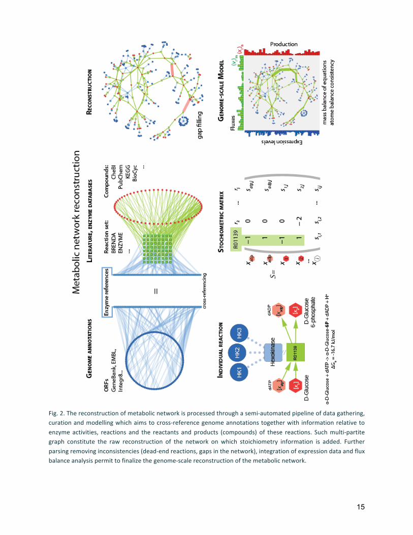
Fig. 2. The reconstruction of metabolic network is processed through a semi-‐automated pipeline of data gathering, curation and modelling which aims to cross-‐reference genome annotations together with information relative to enzyme activities, reactions and the reactants and products (compounds) of these reactions. Such multi-‐partite graph constitute the raw reconstruction of the network on which stoichiometry information is added. Further parsing removing inconsistencies (dead-‐end reactions, gaps in the network), integration of expression data and flux balance analysis permit to finalize the genome-‐scale reconstruction of the metabolic network.
16
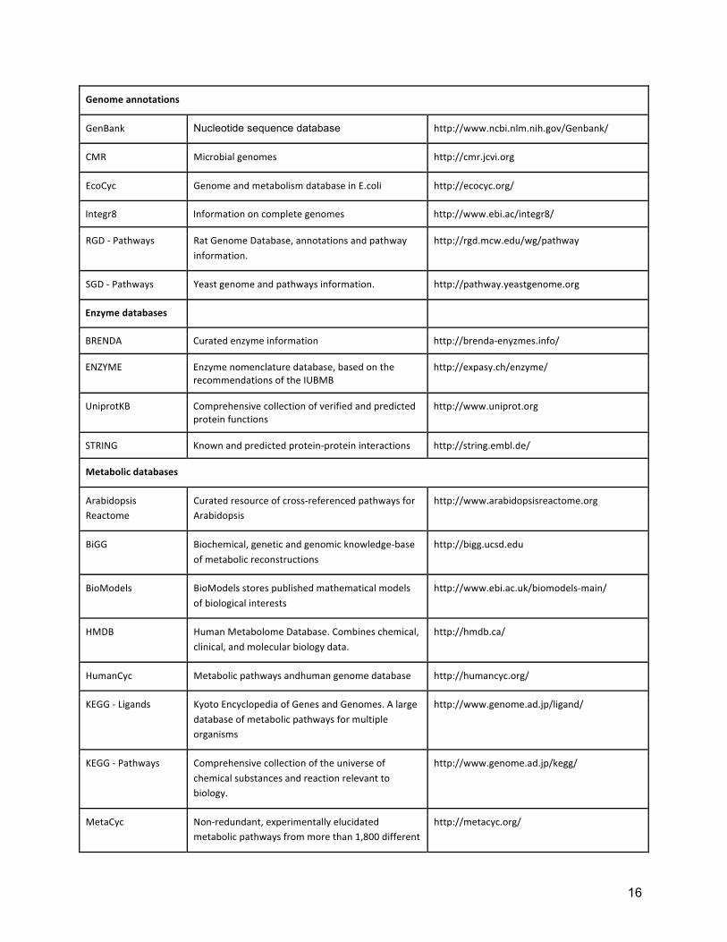
Genome annotations
GenBank Nucleotide sequence database http://www.ncbi.nlm.nih.gov/Genbank/
CMR Microbial genomes http://cmr.jcvi.org
EcoCyc Genome and metabolism database in E.coli http://ecocyc.org/
Integr8 Information on complete genomes http://www.ebi.ac/integr8/
RGD -‐ Pathways Rat Genome Database, annotations and pathway information.
http://rgd.mcw.edu/wg/pathway
SGD -‐ Pathways Yeast genome and pathways information. http://pathway.yeastgenome.org
Enzyme databases
BRENDA Curated enzyme information http://brenda-‐enyzmes.info/
ENZYME Enzyme nomenclature database, based on the recommendations of the IUBMB
http://expasy.ch/enzyme/
UniprotKB Comprehensive collection of verified and predicted protein functions
http://www.uniprot.org
STRING Known and predicted protein-‐protein interactions http://string.embl.de/
Metabolic databases
Arabidopsis Reactome
Curated resource of cross-‐referenced pathways for Arabidopsis
http://www.arabidopsisreactome.org
BiGG Biochemical, genetic and genomic knowledge-‐base of metabolic reconstructions
http://bigg.ucsd.edu
BioModels BioModels stores published mathematical models of biological interests
http://www.ebi.ac.uk/biomodels-‐main/
HMDB Human Metabolome Database. Combines chemical, clinical, and molecular biology data.
http://hmdb.ca/
HumanCyc Metabolic pathways andhuman genome database http://humancyc.org/
KEGG -‐ Ligands Kyoto Encyclopedia of Genes and Genomes. A large database of metabolic pathways for multiple organisms
http://www.genome.ad.jp/ligand/
KEGG -‐ Pathways Comprehensive collection of the universe of chemical substances and reaction relevant to biology.
http://www.genome.ad.jp/kegg/
MetaCyc Non-‐redundant, experimentally elucidated metabolic pathways from more than 1,800 different
http://metacyc.org/

17
organisms
MetExplore A web server to link metabolomic experiments and genome-‐scale metabolic
http://metexplore.toulouse.inra.fr/metexplore/
MouseCyc Mice metabolic pathways and genome database http://mousecyc.jax.org/
PlantCyc Plant Metabolic Networks http://www.plantcyc.org/
Pubchem Small molecules database http://pubchem.ncbi.nlm.nih.gov
Reactome Curated database of metabolic pathways http://www.reactome.org/
SMPDB Human Small Molecule Pathway Database http://www.smpdb.ca/
Repositories of experimental data
Array Express Microarrays database http://www.ebi.ac.uk/aerep/
DIP Protein-‐protein interactions experimentally determined
http://dip.doe-‐mbi.ucla.edu/
GEO Microarrays database http://www.ncbi.nlm.nih.gov/geo/
IntAct Reported protein-‐protein interactions http://www.ebi.ac.uk/intact/
Tools for automated reconstruction
Pathway tools Uses MetatCyc pathway database http://bioinformatics.ai.sri.com/ptools/
Table 1: Main sources of metabolic pathways and networks.
Name Description url
CARMEN Comparative Analysis and Reconstruction of MEtabolic Networks
http://carmen.cebitec.uni-‐bielefeld.de/cgi-‐bin/index.cgi
MFinder Network motif finder http://www.weizmann.ac.il/mcb/UriAlon/groupNetworkMotifSW.html
FanMod Network motif finder http://www.minet.uni-‐jena.de/\~wernicke/motifs/
Clique Finder Clique identifier http://topnet.gersteinlab.org/clique/
MCODE Cluster finder http://cbio.mskcc.org/\~bader/software/mcode/index.html
Cytoscape Network visualization and advanced analysis
http://www.cytoscape.org/

18
Vanted Network analysis http://vanted.ipk-‐gatersleben.de/
NeAT Network analysis comparison randomization
http://rsat.ulb.ac.be/rsat/index\_neat.html
TYNA Network analysis http://tyna.gersteinlab.org/tyna/
NCT Network comparison, randomization
http://chianti.ucsd.edu/nct/
R/Bioconductor Network analysis packages for R http://www.bioconductor.org/
Cell Net Analyzer Structural and functional analysis of metabolic and cellular networks
http://www.mpi-‐magdeburg.mpg.de/projects/cna/cna.html
13CFlux Software toolkit for isotope-‐based metabolic flux analysis.
https://www.13cflux.net/
Table 2: Software for network data analysis and representation.
Cross-‐References 1. KEGG (00472) 2. Metabolic Network and their evolution (0004) 3. Modularity (00475) 4. Multi-‐Output FFLs (00555) 5. Network Alignments (0482)
References 1. Adam M Feist, Markus J Herrgrd, Ines Thiele, Jennie L Reed, and Bernhard Palsson. Reconstruction of biochemical networks in microorganisms. Nat Rev Microbiol, 7(2):129–143, Feb 2009. 2. Bernhard O. Palsson. Systems biology: properties of reconstructed networks. Cambridge University Press, 1st edition, January 2006. 3. Eytan Ruppin, Jason A Papin, Luis F de Figueiredo, and Stefan Schuster. Metabolic reconstruction, constraint-‐based analysis and game theory to probe genome-‐scale metabolic networks. Curr Opin Biotechnol, 21(4):502–510, Aug 2010.

19
Flux Balance Analysis Synonyms FBA, flux coupling analysis, fluxomics. Definition Flux balance analysis (FBA) is a widely used method to study genome-‐scale metabolic networks (See Metabolic networks, structure and dynamics). The FBA method is used to calculate the flux of metabolites that can maximize – or minimize – a concentrations of species of interest in a given network. For instance, it and can be used to compute the theoretical maximum growth rate of an organism given a particular state of its metabolism(1). FBA is limited to steady-‐state solutions, and therefore does not require to know a priori the concentrations of metabolites or the kinetic parameters of the enzymes contained in the network of interest. Moreover, the computation of the method is straightforward and relatively not demanding in resources. Procedure Let us suppose a metabolic network G(m, n) that comprises of m metabolites and n catalytic reactions: all the metabolic reactions can be represented in a stoichiometric matrix S in which the entries give the stoichiometric coefficient of the compounds (rows) for each reaction (columns). (See Stoichiometry matrix). In addition, the concentrations of each metabolites are contained in a vector x = (x1 , … , xm ). By definition, the steady-‐state of the metabolic network is reached when the concentration of each compound is steady. In mathematical terms, the equilibrium is reached when:
�i � {1, . . . , m}, dxi/dt =0 (1) # LaTeX code for the equation \begin{equation}\forall i \in \{1,\dots,m\}, \frac{dx_i}{dt}=0 \label{ED1}\end{equation} We can define the flux of each catalytic reaction in the network by the rate vector v = (v1 , . . . , vn ). The vector of fluxes often contains exchange fluxes, denoted bi . Therefore, the condition of the steady-‐state (Eq. 1) is satisfied when:
dx/dt = S ·∙ v = 0 �� (2)
# LaTeX code for the equation: \begin{equation}
\frac{dx}{dt}= S\cdot v=0

20
\iff \bordermatrix{ & & &\cr & s_{1,1} & \dots & s_{1,n}\cr & \vdots & \ddots & \vdots \cr & s_{m,1} &
\dots & s_{m,n} } \cdotp \bordermatrix{ & \cr & v_1\cr & \vdots\cr & v_{m} }=0 \label{ED2}
\end{equation} Any v satisfying (Eq. 2) belongs to the null space of S. In particular, in the context of metabolic networks, there are generally more reactions than metabolites, which means than m > n. It implies that there are no unique solution to this system of equation. As such, it means that the stoichiometric coefficient bracket the range of possible fluxes permitted, but the space of possible solution remains infinite without the use of additional constraints. Yet, the null-‐space of S can be reduced by defining adjustable constraints on the acceptable values of the fluxes, in accordance with biologically realistic values: for instance, a given vi might be constrained in a positive and finite interval (0 ≤ vi ≤ vmax ). Experimentally determined fluxes can also be used to define accurate constraints that can range in a defined interval (vexp − ε ≤ vi ≤ vexp + −ε). The addition of constraints, however, is not sufficient to reduce the space of solutions to a unique solution. Linear programming is therefore used to generate a single optimal flux for a given objective. This can be determined by applying weights on the set of n reactions in order to reach a given objective. This requires to define a vector of weights w = (w1 , … , wn ) such that:
< w ·∙ v > = (3) # LaTeX code for the equation \begin{equation} <w \cdot v> = \sum_{i=1}^n w_i v_i= Z\label{ED3}\end{equation} where Z gives a direction in (v1 , … , vn ), and is called the objective function. By resolving (Eq.3) within the space of allowed flux given by (Eq.2), the FBA renders a vector of flux vf that correspond to a steady-‐state compatible with the objective. For example, the vector w can be defined to optimize a single flux (e.g. vAT Pmax to maximize the production of ATP). Classical objective functions might also be defined to optimize the biomass formation, the adaptation to a given stress (e.x. anaerobic stress), nutrient uptake, or production of a gene of interest. See also Metabolic networks, structure and dynamics and (2). Cross-‐References 1. KEGG (00472) 2. Metabolic Network and their evolution (0004)

21
3. Modularity (00475) 4. Multi-‐Ouput FFLs (00555) 5. Network Alignments (0482)
Name URL
COBRA Toolbox http://gcrg.ucsd.edu/Downloads/Cobra_Toolbox
FCF http://maranas.che.psu.edu/
MOMA http://arep.med.harvard.edu/moma
OptFlux http://www.optflux.org/
Table 1 -‐ Computational tools for flux balance analysis
References 1. J. S. Edwards, R. U. Ibarra, and B. O. Palsson. In silico predictions of escherichia coli metabolic capabilities are consistent with experimental data. Nat Biotechnol, 19(2):125–130, Feb 2001. 2. Jeffrey D Orth, Ines Thiele, and Bernhard Palsson. What is flux balance analysis? Nat Biotechnol, 28(3):245–248, Mar 2010.
22
Clustering coefficient
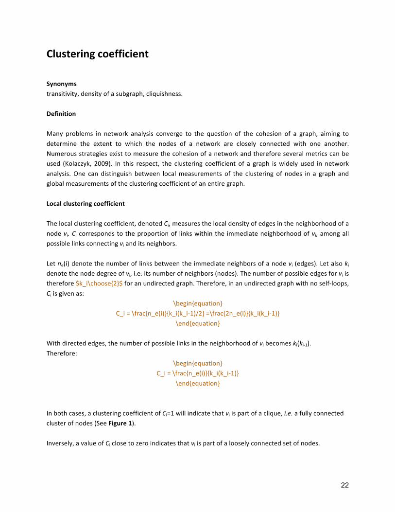
Synonyms transitivity, density of a subgraph, cliquishness. Definition Many problems in network analysis converge to the question of the cohesion of a graph, aiming to determine the extent to which the nodes of a network are closely connected with one another. Numerous strategies exist to measure the cohesion of a network and therefore several metrics can be used (Kolaczyk, 2009). In this respect, the clustering coefficient of a graph is widely used in network analysis. One can distinguish between local measurements of the clustering of nodes in a graph and global measurements of the clustering coefficient of an entire graph. Local clustering coefficient The local clustering coefficient, denoted Ci, measures the local density of edges in the neighborhood of a node vi. Ci corresponds to the proportion of links within the immediate neighborhood of vi, among all possible links connecting vi and its neighbors. Let ne(i) denote the number of links between the immediate neighbors of a node vi (edges). Let also ki denote the node degree of vi, i.e. its number of neighbors (nodes). The number of possible edges for vi is therefore $k_i\choose{2}$ for an undirected graph. Therefore, in an undirected graph with no self-‐loops, Ci is given as:
\begin{equation} C_i = \frac{n_e(i)}{k_i(k_i-‐1)/2} =\frac{2n_e(i)}{k_i(k_i-‐1)}
\end{equation} With directed edges, the number of possible links in the neighborhood of vi becomes ki(ki-‐1). Therefore:
\begin{equation} C_i = \frac{n_e(i)}{k_i(k_i-‐1)}
\end{equation} In both cases, a clustering coefficient of Ci=1 will indicate that vi is part of a clique, i.e. a fully connected cluster of nodes (See Figure 1). Inversely, a value of Ci close to zero indicates that vi is part of a loosely connected set of nodes.
23
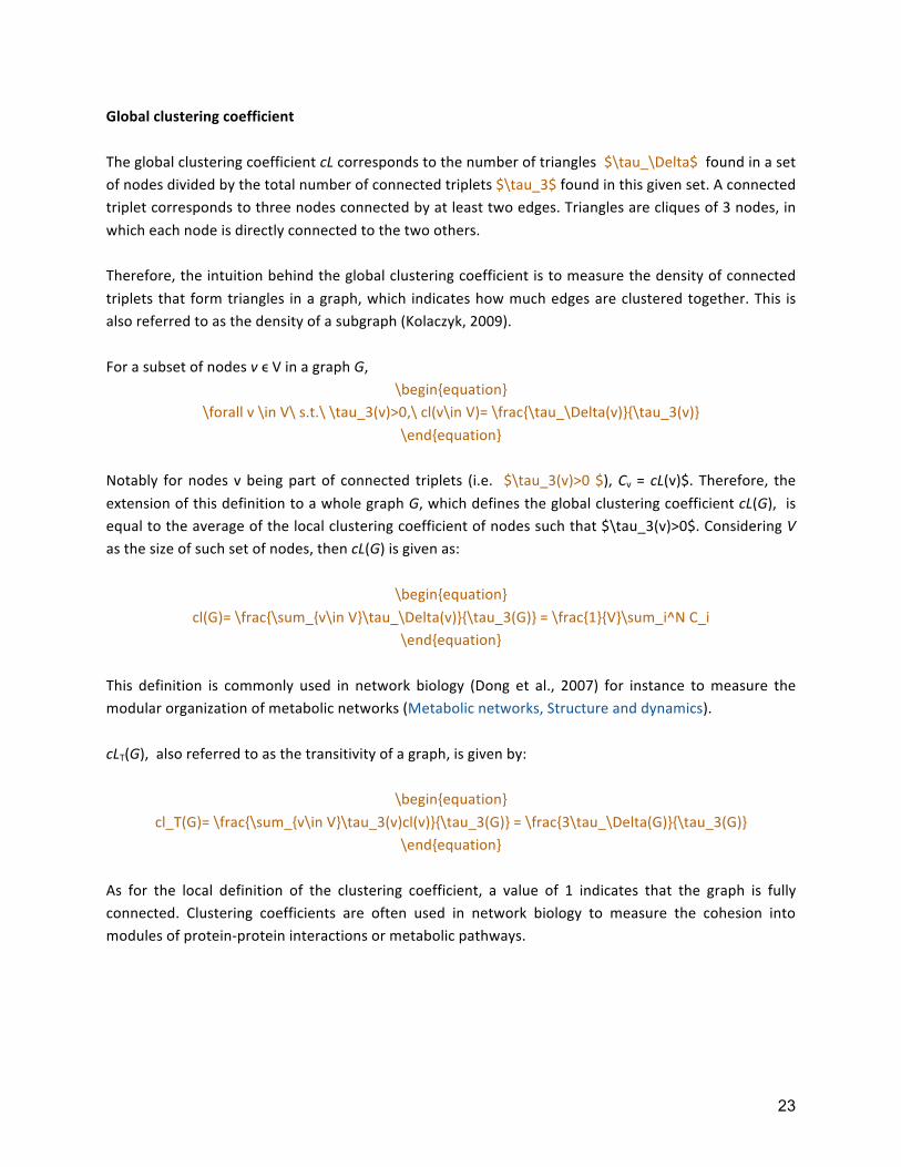
Global clustering coefficient The global clustering coefficient cL corresponds to the number of triangles $\tau_\Delta$ found in a set of nodes divided by the total number of connected triplets $\tau_3$ found in this given set. A connected triplet corresponds to three nodes connected by at least two edges. Triangles are cliques of 3 nodes, in which each node is directly connected to the two others. Therefore, the intuition behind the global clustering coefficient is to measure the density of connected triplets that form triangles in a graph, which indicates how much edges are clustered together. This is also referred to as the density of a subgraph (Kolaczyk, 2009). For a subset of nodes v ϵ V in a graph G,
\begin{equation} \forall v \in V\ s.t.\ \tau_3(v)>0,\ cl(v\in V)= \frac{\tau_\Delta(v)}{\tau_3(v)}
\end{equation}
Notably for nodes v being part of connected triplets (i.e. $\tau_3(v)>0 $), Cv = cL(v)$. Therefore, the extension of this definition to a whole graph G, which defines the global clustering coefficient cL(G), is equal to the average of the local clustering coefficient of nodes such that $\tau_3(v)>0$. Considering V as the size of such set of nodes, then cL(G) is given as:
\begin{equation} cl(G)= \frac{\sum_{v\in V}\tau_\Delta(v)}{\tau_3(G)} = \frac{1}{V}\sum_i^N C_i
\end{equation}
This definition is commonly used in network biology (Dong et al., 2007) for instance to measure the modular organization of metabolic networks (Metabolic networks, Structure and dynamics). cLT(G), also referred to as the transitivity of a graph, is given by:
\begin{equation} cl_T(G)= \frac{\sum_{v\in V}\tau_3(v)cl(v)}{\tau_3(G)} = \frac{3\tau_\Delta(G)}{\tau_3(G)}
\end{equation} As for the local definition of the clustering coefficient, a value of 1 indicates that the graph is fully connected. Clustering coefficients are often used in network biology to measure the cohesion into modules of protein-‐protein interactions or metabolic pathways.

24
Fig. 1. The density of connections in a graph can be approached by local and global definitions of the clustering coefficient. The local clustering coefficient represents the density of connections among the neighbors of a node, and ranges from 0 to 1. The higher the value, the more the node is part of a densely connected cluster of nodes. The Global definition relates to the proportion of triplets that form triangles in a graph. The density corresponds to the mean value of the local clustering coefficient, while the transitivity of a graph gives the probability that the direct neighbors of a node are connected.
Cross-‐References Metabolic Networks, structure and dynamics.
References 1. Jun Dong and Steve Horvath. Understanding network concepts in modules. BMC Syst Biol, 1:24, 2007. 2. E.D. Kolaczyk. Statistical analysis of network data. Number XII. Springer Series in Statistics,2009.