allocation of unidentified gas revised … · revised allocation of unidentified gas statement for...
TRANSCRIPT

ALLOCATION OF UNIDENTIFIED GAS
Revised Allocation of Unidentified Gas Statement
for 2017/18 Xoserve Ltd
Report No.: 16819, Rev. 2
Date: 28th April 2017
DNV GL – Report No. 16819, Rev. 2 – www.dnvgl.com Page i
Project name: Allocation of Unidentified Gas DNV GL - Software
Software Consulting
Holywell Park
Ashby Road
Loughborough
LE11 3GR
Tel: +44 (0)1509 282000
Report title: Revised Allocation of Unidentified Gas Statement
for 2017/18
Customer: Xoserve Ltd
Customer contact: Fiona Cottam
Date of issue: 28th April 2017
Project No.: 4009457
Organisation unit: Software
Report No.: 16819, Rev. 2
Objective: This document is the revised AUG Statement for 2017/18 and contains details of the methods
developed by the AUG Expert for allocating daily UG between Product Class/EUC including details of the
data requested to support this analysis, data received following such requests and any assumptions
made. This document is an update to the first draft AUG Statement to incorporate changes following the
industry consultation period. This document also contains an updated estimate of the AUG weighting
factors based on the changes made to the methodology.
Prepared by: Verified by: Approved by:
Andy Gordon
Senior Consultant
Tony Perchard
Principal Consultant
Anthony Gilbert
Bespoke and Technical Solution Delivery Manager
Mark Lingham
Senior Consultant
Clive Whitehand
Head of Section
Copyright © DNV GL 2017. All rights reserved. This Report is protected by copyright and may not be reproduced in whole or in part by
any means without the approval in writing of DNV GL. No Person, other than the Customer for whom it has been prepared, may place
reliance on its contents and no duty of care is assumed by DNV GL toward any Person other than the Customer. This Report must be
read in its entirety and is subject to any assumptions and qualifications expressed therein. Elements of this Report contain detailed
technical data which is intended for analysis only by persons possessing requisite expertise in its subject matter. DNV GL and the Horizon Graphic are trademarks of DNV GL AS.
DNV GL Distribution: Keywords:
☒ Unrestricted distribution (internal and external) Unidentified Gas, AUGE, AUGS
☐ Unrestricted distribution within DNV GL Group
☐ Unrestricted distribution within DNV GL contracting party
☐ No distribution (confidential)

DNV GL – Report No. 16819, Rev. 2 – www.dnvgl.com Page ii
Rev. No. Date Reason for Issue Prepared by Verified by Approved by
1 2017-02-01 First draft Andy Gordon & Mark
Lingham
Tony Perchard &
Clive Whitehand
Anthony Gilbert
2 2017-04-28 Revised version Andy Gordon & Mark
Lingham
Tony Perchard &
Clive Whitehand
Anthony Gilbert
DNV GL – Report No. 16819, Rev. 2 – www.dnvgl.com Page iii
EXECUTIVE SUMMARY
Project Nexus is currently scheduled for implementation in readiness for the 2017 gas year. This involves
the replacement of key IT systems (‘UKLink’) for gas settlement and supply point administration in the
gas industry and changes the way that the gas settlement is handled. Project Nexus will introduce
individual meter point reconciliation for all meter points including those on CSEPs (previously SSP meters
were subject to reconciliation by difference) and a rolling monthly AQ process. It also introduces 4 new
meter point ‘classes’.
As a result of these changes, there is a requirement to fairly apportion the daily total UG estimate
between Product Classes and EUC. Mod 0473 was raised to allow the appointment of an independent
expert (AUG Expert) to develop a methodology to do this and provide a table of weighting factors that
will target the correct amount of UG to different classes of meter points, based on an assessment of their
relative contribution to UG. The table of weighting factors will be used in the daily gas nomination and
allocation processes.
This document is the revised AUG Statement for 2017/18 and contains details of the methods developed
by the AUG Expert for allocating daily UG between Product Class/EUC including details of the data
requested to support this analysis, data received following such requests and any assumptions made.
This document also contains the latest estimate of the AUG weighting factors.
This document follows a 42 day consultation period, which allowed the industry to provide feedback to
the AUG Expert and raise questions/issues on the first draft. Where appropriate, the methodology has
been updated based on this feedback.
In addition to the above, this document describes how the AUG Expert has followed the published
guidelines.

DNV GL – Report No. 16819, Rev. 2 – www.dnvgl.com Page iv
TABLE OF CONTENTS
EXECUTIVE SUMMARY ............................................................................................................ III
1 INTRODUCTION ............................................................................................................... 1
1.1 Background ............................................................................................................... 1
1.2 High Level Objectives.................................................................................................. 1
1.3 Scope ....................................................................................................................... 2
2 COMPLIANCE TO GENERIC TERMS OF REFERENCE ............................................................ 3
3 HIGH LEVEL OVERVIEW OF METHODOLOGY ..................................................................... 6
3.1 LDZ Load Components ................................................................................................ 6
3.1.1 Pre-Nexus Regime ......................................................................................... 6
3.1.2 Post-Nexus Regime ....................................................................................... 6
3.1.3 Unidentified Gas ............................................................................................ 8
3.2 Permanent and Temporary Unidentified Gas .................................................................. 8
3.3 Unidentified Gas Methodology ...................................................................................... 9
3.3.1 Estimation of Total UG for Historic Years .......................................................... 9
3.3.2 Calculating Components of Total UG .............................................................. 10
3.3.3 Mapping to Post-Nexus Product Classes ......................................................... 13
3.3.4 Projection of Permanent UG to Forecast Period................................................ 14
3.3.5 Unidentified Gas Factors .............................................................................. 15
4 SUMMARY OF ANALYSIS................................................................................................. 17
5 DATA USED..................................................................................................................... 18
5.1 Summary ................................................................................................................ 18
5.2 Total UG Calculation (Consumption Method) ................................................................ 19
5.3 IGT CSEP Setup and Registration Delays ..................................................................... 20
5.4 Unregistered/Shipperless Sites ................................................................................... 20
5.5 Meter Errors ............................................................................................................ 22
5.6 Theft ...................................................................................................................... 22
5.7 Shrinkage ................................................................................................................ 22
6 METHODOLOGY .............................................................................................................. 23
6.1 Correcting the NDM Allocation .................................................................................... 23
6.1.1 Known DM and LDZ Metering Errors .............................................................. 23
6.1.2 Shrinkage Error .......................................................................................... 24
6.2 NDM Consumption Calculation.................................................................................... 24
6.2.1 Algorithm ................................................................................................... 24
6.2.2 Aggregation and Scaling-Up ......................................................................... 30
6.3 Unregistered and Shipperless Sites ............................................................................. 34
DNV GL – Report No. 16819, Rev. 2 – www.dnvgl.com Page v
6.4 IGT CSEPs ............................................................................................................... 40
6.4.1 Overview.................................................................................................... 40
6.4.2 Data .......................................................................................................... 40
6.4.3 Process ...................................................................................................... 41
6.5 Consumer Metering Errors ......................................................................................... 43
6.6 Detected Theft ......................................................................................................... 46
6.7 Shrinkage Issues ...................................................................................................... 47
6.8 Balancing Factor ....................................................................................................... 48
6.9 Extrapolation to Forecast Period ................................................................................. 50
6.10 UG Factor Calculation ................................................................................................ 54
7 UNIDENTIFIED GAS FACTORS ........................................................................................ 55
8 CONSULTATION QUESTIONS AND ANSWERS .................................................................. 56
9 CONTACT DETAILS ......................................................................................................... 56
10 REFERENCES .................................................................................................................. 57
GLOSSARY .............................................................................................................................. 58
Appendix A Data
DNV GL – Report No. 16819, Rev. 2 – www.dnvgl.com Page vi
LIST OF FIGURES
Figure 1: NDM Allocation and Unidentified Gas ................................................................................ 9
Figure 2: Calculation of Unidentified Gas from Consumptions and Allocations .................................... 10
Figure 3: UG Components ........................................................................................................... 13
Figure 4: Projecting UG .............................................................................................................. 15
Figure 5: Consumption Algorithm Flow Chart ................................................................................. 25
Figure 6: Meter Read Availability Scenarios ................................................................................... 27
Figure 7: Consumption Method used for each type of Meter Point .................................................... 32
Figure 8: Piecewise Trend for Unregistered UG, Training and Forecast .............................................. 37
Figure 9: iGT CSEPs UG by Snapshot ............................................................................................ 43
Figure 10: Typical Calibration Curve for an RPD Meter .................................................................... 44
Figure 11: Percentage of Theft Detections by Year Number ............................................................. 47
Figure 12: Balancing Factor by Year ............................................................................................. 53
LIST OF TABLES
Table 1: Product Classes ............................................................................................................... 7
Table 2: Example UG Weighting Factor Table .................................................................................. 7
Table 3: Product Class Assignment Key Parameters ....................................................................... 14
Table 4: Data Status Summary .................................................................................................... 19
Table 5: Unknown Projects Snapshot ............................................................................................ 42
Table 6: Balancing Factor Split .................................................................................................... 50
Table 7: Draft Unidentified Gas Weighting Factors .......................................................................... 55
Table 8: Responses to the First Draft of the 2017/18 AUG Statement ............................................... 56
DNV GL – Report No. 16819, Rev. 2 – www.dnvgl.com Page 1
1 INTRODUCTION
1.1 Background
The majority of gas consumed in Great Britain is metered and registered. However, some gas is lost
from the system, or not registered, due to theft, leakage from gas pipes, consumption by Unregistered
supply points and other reasons. Some elements of the gas that is not directly consumed/measured are
currently modelled, and hence the gas consumed by these can be estimated. The gas that is lost and not
recorded or modelled is referred to as Unidentified Gas (UG).
Currently, the Great Britain gas industry is segmented into two market sectors; Larger Supply Points
(LSP) and Smaller Supply Points (SSP). Prior to April 2012 there was no methodology in place to
determine the allocation of UG between the LSP and SSP market sectors: UG was ultimately borne by
the SSP market sector following reconciliation (an interim amount was allocated for 2011/12). Through
the approval of UNC Modification 0229 and the appointment of DNV GL as the Allocation of Unidentified
Gas Expert (AUGE) in 2011, a methodology was developed to calculate and apportion UG equitably to
the relevant gas market sectors. This approach involved an annual estimate of UG and a monthly
transfer of costs between market sectors to address the misallocation of UG that occurs under the
current regime. DNV GL carried out this annual process until 2014 when it became clear that the
requirements for the AUGE would change given the upcoming implementation of project ‘Nexus’ (Mod
0432).
Project Nexus involves the replacement of key IT systems (‘UKLink’) for gas settlement and supply point
administration in the gas industry. This is currently scheduled for implementation in readiness for the
2017 gas year and involves a change in the way that gas settlement is handled. Project Nexus will
introduce individual meter point reconciliation for all meter points (previously SSP meters were subject
to reconciliation by difference) and a rolling monthly AQ process. It also introduces 4 new meter point
‘classes’.
After Project Nexus implementation, an amended NDM Algorithm (with scaling factor removed) will use
actual weather data to derive a bottom-up estimate of NDM Demand. This allows the calculation of a
daily total of Unidentified Gas. This UG will be shared out to all live sites, on the basis of their
recorded/estimated throughput for the day.
As a result of these changes, the industry noted a requirement to be able to fairly apportion this total UG
between Product Classes and EUC. Mod 0473 was raised to allow the appointment of an independent
expert (the AUG Expert) to develop a methodology to do this and provide a table of weighting factors
that will assign the correct amount of UG to different classes of meter points, based on an assessment of
their relative contribution to UG. The table of weighting factors will be used in daily gas allocation
processes. Daily measured or estimated gas throughput in each sector will be weighted using the AUG
table factors to assign daily UG to Shippers based on their throughput by meter point class and EUC.
Mod 0473 was approved for implementation on the Project Nexus go-live date. DNV GL were appointed
to the new role of AUG Expert in July 2016.
1.2 High Level Objectives
The AUG Expert’s high level objectives are:
To assess the sources of UG and the data available/required from industry bodies to evaluate UG

DNV GL – Report No. 16819, Rev. 2 – www.dnvgl.com Page 2
To gather data as required from Xoserve, from Gas Shippers, or drawn from other sources, as
deemed appropriate by the AUG Expert
To develop the methodology to assess the relative contribution to UG of different Classes and sizes
of sites
To publish the methodology in the AUG Statement (this document) and present findings to the
industry
To consult with the industry bodies and respond to questions/issues raised, assess the impact of
questions on the methodology and update as appropriate
Produce the table detailing the weighting factors for each Product Class and End User Category (EUC)
1.3 Scope
This document is the second draft AUG Statement for 2017/18 and contains the following:
A detailed description of the proposed methodology
A summary of data requested, received and used, and associated assumptions
The table of weighting factors for apportioning UG between Product Classes and EUCs
Details of the database used to hold information associated with UG and used to develop the
methodology
This document will be published to the industry for review and comment during the consultation period.
The following are out of scope.
The AUG Expert is not concerned with issues regarding the deeming algorithm or the RbD
mechanism.
The AUG Expert is not concerned with resolution of fundamental gas industry business process
issues.
The AUG Expert process is not an opportunity to provide permanent solutions to issues within
the gas industry that should be addressed by other workgroups (e.g. Shrinkage Forum).
The AUG Expert is not concerned with transportation charges.
DNV GL – Report No. 16819, Rev. 2 – www.dnvgl.com Page 3
2 COMPLIANCE TO GENERIC TERMS OF REFERENCE
This section describes how DNV GL has adhered to the Generic Terms of Reference described in Section
5 of the AUGE Guidelines [1].
The AUG Expert will create the AUG Statement by developing appropriate, detailed
methodologies and collecting necessary data.
The AUG Expert has developed a detailed methodology for estimating factors to apportion UG between
EUC and Product Classes. To calculate the factors, total UG is also estimated using meter read and
consumption data for all meters, which has been obtained from Xoserve. Further detailed datasets are
used to directly estimate some components of the total UG where this is possible e.g. Shipperless sites.
The AUG Expert has also developed a methodology to account for elements of UG which are Temporary
in nature.
Additional data regarding theft of gas and likely take up rates of Product Classes was sought from the
industry. Requests for information were also submitted to the Theft Risk Assessment Service (TRAS)
and Smart Energy GB.
The decision as to the most appropriate methodologies and data will rest solely with the AUG
Expert taking account of any issues raised during the development and compilation of the
AUG Statement.
The proposed methodology and assessment of what constitutes UG has been decided solely by the AUGE
based on available information. Comments raised by shippers relating to the AUG Statement have been
considered and responses issued as part of the consultation process. Having considered all views, the
final decisions are the AUG Expert’s own.
The AUG Expert will determine what data is required from Code Parties (and other parties as
appropriate) in order to ensure appropriate data supports the evaluation of Unidentified Gas.
The AUG Expert has assessed what data is required to support the proposed methodology and has
requested information from relevant parties. For the 2016 analysis, updated data sets have been
requested from Xoserve for all items.
The AUG Expert will determine what data is available from parties in order to ensure
appropriate data supports the evaluation of Unidentified Gas.
The AUG Expert has determined what data is available following discussions with Xoserve. A request
was also made to shippers to establish if further information is available regarding theft and potential
uptake of Product Classes.
The AUG Expert will determine what relevant questions should be submitted to Code Parties
in order to ensure appropriate methodologies and data are used in the evaluation of
unidentified error.
Questions regarding the relative ease of theft and detection of theft from Smart Meters vs mechanical
meters have been submitted to the industry. Further communication will take place as and when
necessary.
The AUG Expert will use the latest data available where appropriate.
Xoserve have provided all the latest available data as requested by the AUG Expert. Further updates will
be provided if available for use in the calculation of the final table of factors.

DNV GL – Report No. 16819, Rev. 2 – www.dnvgl.com Page 4
Where multiple data sources exist the AUG Expert will evaluate the data to obtain the most
statistically sound solution, will document the alternative options and provide an explanation
for its decision.
For the consumption method of estimating total UG, both meter reads and metered volumes are
provided. Over time LSP metered volumes may be corrected, but the meter reads are not. The AUG
Expert’s analysis has shown that metered volumes can be erroneous, particularly for non-corrected SSP
data. The decision was therefore taken to use meter reads for SSP and metered volumes for LSP.
Where data is open to interpretation the AUG Expert will evaluate the most appropriate
methodology and provide an explanation for the use of this methodology.
Throughout the statement the AUG Expert has described how data will be used and why.
Where the AUG Expert considers using data collected or derived through the use of sampling
techniques, then the AUG Expert will consider the most appropriate sampling technique
and/or the viability of the sampling technique used.
The consumption method for estimating the UG total is the only part of the analysis where a sample
rather than the full dataset is used. This calculation will be at its most accurate when the largest
possible representative subset of the meter point population is used. To achieve this, a validation
process was developed that was designed to maximise the sample size whilst removing any meter points
with invalid data. Appropriate methods are then applied to scale up for any meter points which have
been excluded.
The AUG Expert will present the AUG Statement in draft form (the “Draft AUG Statement”), to
Code Parties seeking views and will review all the issues identified submitted in response.
The AUG Expert has documented and reviewed all feedback resulting from previous versions of the AUG
Statement. Section 8 of this document refers to these publications with details of the issues raised, with
the full text of the comments from the Code Parties and the AUG Expert responses contained in separate
documents published on the Joint Office of Transporters website.
The AUG Expert will provide the Draft and final AUG Statement to the Gas Transporters for
publication.
This 2nd draft AUGS for 2017/18 is provided to the Gas Transporters for publication on 30th April 2017.
The Committee’s final determination in this process shall be binding on Users.
This section is not relevant to AUG Expert.
The AUG Expert will undertake to ensure that all data that is provided to it by all parties will
not be passed on to any other organisation, or used for any purpose other than the creation of
the methodology and the AUG Statement.
On receipt of data, the AUG Expert stores the data in a secure project storage area with limited access
by the consultants working on the project. The AUG Expert can confirm data used in the analysis has
not and will not be passed on to any other organisation. The data used will be made available to all
bona fide industry participants in order to review the methodology, and in this dataset all MPR
information has been replaced by ‘dummy’ MPR references by Xoserve so that the anonymity of the
consumer is protected.

DNV GL – Report No. 16819, Rev. 2 – www.dnvgl.com Page 5
The AUG Expert shall ensure that all data provided by Code Parties will be held confidentially,
and where any data, as provided or derived from that provided, is published then it shall be in
a form where the source of the information cannot be reasonably ascertained.
Data is stored in a secure project storage area with access limited to those working on the project. Any
data that contains market share or code party specific information has been and will be made
anonymous to ensure the source of the information cannot be ascertained.
DNV GL – Report No. 16819, Rev. 2 – www.dnvgl.com Page 6
3 HIGH LEVEL OVERVIEW OF METHODOLOGY
This section provides a high-level overview of the methodology. For each of the areas of UG presented
here a more detailed discussion is given in Section 6.
Under the current settlement regime, an independent forecast of permanent UG split by market sector is
made to allow correct allocation of UG costs. Following implementation of Project Nexus, Unidentified
Gas (referred to as UIG in UNC Section H 2.6.2) is calculated daily as part of the settlement process.
This UIG amount is then apportioned based on the weighting factors calculated by the AUG Expert using
the methodology described in this document.
As part of the AUG methodology, the AUG Expert makes an independent estimate of Unidentified Gas
which is referred to throughout this document as UG. This is not the same as UIG. Costs for Unidentified
Gas are calculated by applying the AUG weighting factors to the UIG calculated by Xoserve.
3.1 LDZ Load Components
The Unidentified Gas calculations described in this report are complicated by the fact that the UG Factors,
which are the ultimate output of the work, are required to be split by post-Nexus market sector
definitions, whilst all currently available information and data is from the existing regime with its
associated market sectors. The load components are different in these two scenarios, and this creates a
requirement to map from one to the other in as accurate a manner as possible as part of the calculation
process.
Therefore, the analysis deals with both load components as they exist under the current regime and load
components as they will exist post-Nexus, and so both are described in this section.
3.1.1 Pre-Nexus Regime
Daily load (as measured or calculated at the Supply Meter Point) falls into three relevant categories as
far as the reconciliation process is concerned. These are as defined in Section A of the Uniform Network
Code (UNC) [2]:
1. Smaller Supply Point Component Load
Load from Supply Point Components (SPCs) which are part of a Smaller Supply Point (SSP). This
is defined as a supply point where the AQ is not greater than 73,200 kWh.
2. Larger Non-Daily Metered Supply Point Component Load
Load from Non-Daily Metered (NDM) SPCs which are part of a Larger Supply Point (LSP). This is
defined as a supply point where the AQ is greater than 73,200 kWh but less than the mandatory
daily metering threshold of 58,600,000 KWh. Note that historically (prior to the implementation
of Mod 0428), Larger NDM SPCs may have contained individual meters that fell below the SSP
AQ threshold.
3. Daily Metered Supply Point Component (DM SPC) Load
Load from Daily Metered (DM) SPCs. This includes Daily Metered Mandatory (DMM) sites, which
are those above the 58,600,000 kWh threshold, Daily Metered Voluntary (DMV) and Daily
Metered Elective (DME) sites.
3.1.2 Post-Nexus Regime
Following Project Nexus implementation, the population of supply points will instead be split into four
different Product Classes, each of which have different meter read frequency requirements and

DNV GL – Report No. 16819, Rev. 2 – www.dnvgl.com Page 7
reconciliation rules. A list of products and associated details (including approximate equivalence to
current services) is shown in the table below. Information in this table is taken from UNC Modification
0432 [3].
Process Description
Basis of Energy Allocation
Basis of Energy Balancing
Shipper Read Submission
Market Sector
Current Service Equivalent
Product 1: Daily Metered Time Critical Readings
Daily Read Daily Read Daily by 11 am on GFD+1
DM DM Mandatory
Product 2: Daily Metered not Time Critical Readings
Daily Read Daily Read Daily by end of GFD+1
DM DM Voluntary / DM Elective
Product 3:
Batched Daily Readings
Allocation
Profiles
Allocation
Profiles
Periodically in
batches of daily readings
NDM Non-Daily
Metered
Product 4: Periodic Readings
Allocation Profiles
Allocation Profiles
Periodically NDM Non-Daily Metered
Table 1: Product Classes
Post-Nexus, each site will be classified as subscribing to one of these products, and meter read
submissions, settlement and reconciliation will then be carried out for each site in the manner suitable
for its Product Class.
In addition to splitting the UG figure between the four products, Mod 0473 also includes a requirement to
include a split between End User Categories (EUCs) [4]. The final output of the AUGE process will
therefore be a table of UG factors with the following structure:
Supply Meter Point
Classification
Unidentified Gas Weighting Factor
Class 1 Class 2 Class 3 Class 4
EUC Band 1
EUC Band 2
EUC Band 3
EUC Band 4
EUC Band 5
EUC Band 6
EUC Band 7
EUC Band 8
EUC Band 9
Table 2: Example UG Weighting Factor Table

DNV GL – Report No. 16819, Rev. 2 – www.dnvgl.com Page 8
3.1.3 Unidentified Gas
DM load (Product Classes 1 and 2 post-Nexus) is, by definition, metered and known on an ongoing daily
basis. Like all metered load it can be subject to metering error, and data for known errors is used to
correct it. NDM load (Product Classes 3 and 4 post-Nexus) for a given day can be estimated from
available meter reads (and corrections). This uses a method based on the NDM deeming algorithm, to
which reconciliation is applied when the meter readings become available. The estimation process is
described in Section H of the UNC for the current regime [2] and Mod 0432 for Project Nexus [3].
The sum of these load components does not equal the gas intake into the LDZ due to the presence of
two further factors:
1. Shrinkage
LDZ shrinkage occurs between the LDZ offtake and the end consumer (but not at the Supply Meter
Point - the LDZ shrinkage zone stops immediately before this point). It covers:
Leakage (from pipelines, services, AGIs and interference damage)
Own Use Gas
Transporter-responsible theft
The majority of shrinkage is due to leakage, and the overall LDZ shrinkage quantity is calculated
using the standard method defined in the UNC [2].
2. Unidentified Gas
UG occurs downstream of shrinkage, i.e. at the Supply Meter Point. It potentially covers:
Unregistered and Shipperless sites
Independent Gas Transporter Connected System Exit Point (iGT CSEP) setup and registration
delays
Errors in the shrinkage estimate
Shipper-responsible theft
Meter errors – this includes both LDZ offtakes and consumer meters
UG is currently unknown and hence must be estimated.
The relationship between these components of daily load can therefore be expressed as follows:
Total UG = Aggregate LDZ Load – DM Load – Shrinkage – NDM Load (3.1a)
This can be reformulated for the post-Nexus regime as:
Total UG = Aggregate LDZ Load – Product 1 to 4 Load – Shrinkage (3.1b)
3.2 Permanent and Temporary Unidentified Gas
Unidentified gas can be divided into two categories:
Permanent UG is consumed in an unrecorded fashion and costs are never recovered.
DNV GL – Report No. 16819, Rev. 2 – www.dnvgl.com Page 9
Temporary UG is initially consumed in an unrecorded fashion, but volumes are later calculated directly
or estimated and the cost is recovered via back billing or reconciliation.
3.3 Unidentified Gas Methodology
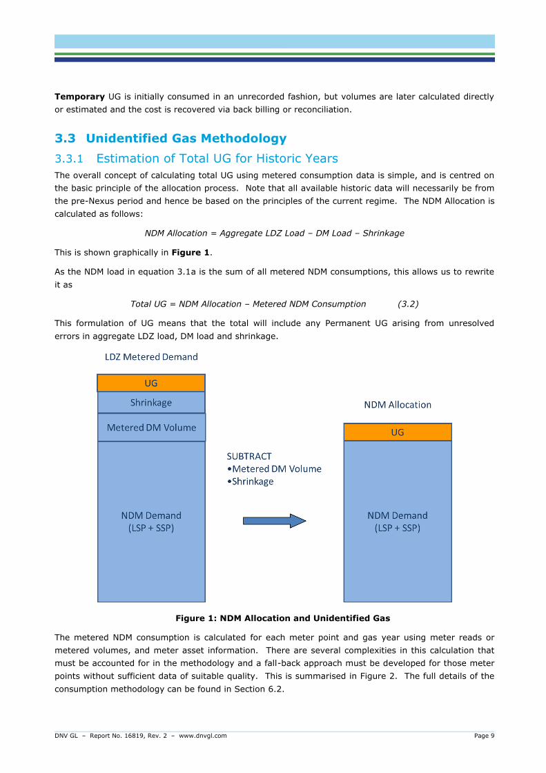
3.3.1 Estimation of Total UG for Historic Years
The overall concept of calculating total UG using metered consumption data is simple, and is centred on
the basic principle of the allocation process. Note that all available historic data will necessarily be from
the pre-Nexus period and hence be based on the principles of the current regime. The NDM Allocation is
calculated as follows:
NDM Allocation = Aggregate LDZ Load – DM Load – Shrinkage
This is shown graphically in Figure 1.
As the NDM load in equation 3.1a is the sum of all metered NDM consumptions, this allows us to rewrite
it as
Total UG = NDM Allocation – Metered NDM Consumption (3.2)
This formulation of UG means that the total will include any Permanent UG arising from unresolved
errors in aggregate LDZ load, DM load and shrinkage.
Figure 1: NDM Allocation and Unidentified Gas
The metered NDM consumption is calculated for each meter point and gas year using meter reads or
metered volumes, and meter asset information. There are several complexities in this calculation that
must be accounted for in the methodology and a fall-back approach must be developed for those meter
points without sufficient data of suitable quality. This is summarised in Figure 2. The full details of the
consumption methodology can be found in Section 6.2.

DNV GL – Report No. 16819, Rev. 2 – www.dnvgl.com Page 10
Figure 2: Calculation of Unidentified Gas from Consumptions and Allocations
This method is used to estimate total UG on a gas year basis. This is initially done on an LDZ by LDZ
basis due to the very high volume of data required (i.e. all meter reads for all sites). The process is
used to estimate the total UG for each of the six most recent historic years for which reliable data is
available. This excludes the most recent year because the number of meters where consumption can be
successfully calculated is much lower due to fewer meter reads being available. The use of data from
this year could therefore be subject to a large degree of uncertainty.
Note that at this stage the total UG figure contains both Permanent and Temporary UG.
3.3.2 Calculating Components of Total UG
Having obtained the total UG figure using the consumption methodology described above, the value of
individual components that make up the UG total are calculated where this is possible. This also includes
the calculation of the amount of this UG which is temporary for each component and how the UG is split
between market sectors. The definition of “market sector” at this stage moves to the post-Nexus one of
products and EUCs. Splitting each directly calculated source of UG by EUC/Product in this way allows
calculations for both the historic period (pre-Nexus) and forecast period (post-Nexus) to be carried out
as follows:
1. Pre-Nexus data is required as a total for each UG component (but split into permanent and
temporary elements). Therefore, the market sector split used does not matter: the output is the sum
of whatever categories are used.
2. The post-Nexus UG forecast must be carried out separately not only for each UG component but
every individual EUC/Product combination within each component. This is because each EUC/Product
combination can follow its own trend over time (depending on market conditions, Mods that have
been created to address individual issues, and so on). Therefore, each must be calculated across the
whole historic period so that the trend can be identified and extrapolated to the forecast period. A
full split into EUC/Product categories is required for this work.
DNV GL – Report No. 16819, Rev. 2 – www.dnvgl.com Page 11
It is known that data for each of the five potential components of UG (Unregistered and Shipperless sites,
iGT errors, shrinkage error, Shipper-responsible theft and metering errors) is available. The availability
and quality of this data varies from component to component, and the AUGE has therefore identified the
best method of calculating each UG component based on the quality of information available for that
component.
Brief descriptions of each UG element are given below.
1. Unregistered and Shipperless Sites
The data available for this element consists of the details for every site that is either Shipperless or
Unregistered at a given point in time. This point in time is the snapshot date, and snapshots are
provided on a monthly basis, allowing the trends in each such UG category to be monitored over
time. The details for each site include AQ, which allows each site to be assigned to the correct EUC
and also allows its gas usage whilst Unregistered/Shipperless to be estimated. Unregistered and
Shipperless sites that contribute to UG are split into the following sub-categories:
Shipper Activity
Orphaned Sites
Unregistered <12 Months
Shipperless Passed to Shipper (PTS)
Shipperless Shipper Specific Report (SSrP)
Sites Awaiting GSR Visit
2. IGT CSEP Setup and Registration Delays
Gas consumed in an unrecorded manner due to iGT CSEP setup and registration delays is also
included in the UG calculation. UG from this source is due to gas networks owned by iGTs but not
present in Xoserve’s records, and also comes from Unregistered sites on known CSEPs. The data
available for this analysis consists of the number and composition of these unknown projects
(number of sites and AQ split by EUC), and the number and AQ of each Unregistered site associated
with a known project. Unknown Project data is again provided in monthly snapshots, allowing trends
over time to be established.
3. Shrinkage Error
Shrinkage errors affect the total UG calculation in that estimated shrinkage is deducted from the LDZ
input total (along with DM load) to give the total NDM allocation from which metered load is then
removed to calculate total UG. The shrinkage estimate comes from the Shrinkage Model, and if this
is biased it will affect the UG estimate.
Shrinkage Model errors are hard to quantify, given that actual shrinkage is unknown and that the
models are built on the most accurate data available. They were trained over 10 years ago, however,
and so the potential exists for inaccuracy to have developed over time. As such, the Gas Retail
Group commissioned a detailed study into this area, which was carried out by Imperial College
Consultants for Energy UK and the report delivered in October 2015 [16]. This report concluded that
due to their age, the models were likely to be under-estimating Shrinkage in the current system, and
concluded that a reasonable estimate of the magnitude of that bias was 20%.
DNV GL – Report No. 16819, Rev. 2 – www.dnvgl.com Page 12
Such a bias will have the effect of inflating the UG total with gas that should have been classed as
Shrinkage, but instead filters through into UG. Without specific action being taken to prevent it, this
would go into the Balancing Factor.
Shrinkage error needs to be split by throughput, however, whilst the Balancing Factor is not.
Therefore it is important to ensure that this element of UG does not reach the Balancing Factor but is
instead estimated and split by throughput separately. This is the approach that is taken, with the
Shrinkage error component estimated independently and taken out of the Balancing Factor. Both the
Shrinkage error and Balancing Factor components then feed into the final UG factor calculations.
4. Shipper-Responsible Theft
Limited reliable data on theft exists, and whilst information for detected and alleged theft is available,
theft by its nature is often undetected. Undetected theft levels are very difficult to quantify
accurately, and estimates from different sources vary widely, from 0.006% of throughput (based on
detected theft only) to around 10%. As it is difficult to accurately estimate theft levels directly,
undetected theft is calculated by subtraction once known levels of detected theft have been
accounted for. Undetected theft is part of the Balancing Factor (see 6 below), and considered over
time, it forms the vast majority of that figure (based on an assumption that Shrinkage error can be
successfully removed from this value).
5. Meter Errors
Meter errors affect UG in different ways depending on their source. Errors in LDZ offtake metering
and DM supply metering affect the estimate of total NDM demand including UG, whilst NDM LSP and
SSP metering errors contribute to UG by affecting the NDM metered total. Corrections are applied to
LDZ offtakes, DM and unique site meters using detected error data supplied by Xoserve. In addition,
the effects of consumer meters (all EUC/Product combinations) under- and over-reading due to
operating at the extremes of their range are modelled and included in the calculations.
6. Balancing Factor
The Balancing Factor is calculated by taking the difference between the calculated total UG and the
sum of the directly estimated components. The Balancing Factor is comprised of UG elements that
cannot be calculated directly because data is either unavailable or unreliable, and is believed to be
mostly undetected theft.
The Permanent component of total UG is then given by the sum of the Balancing Factor and the
Permanent components of the directly calculated components (see Figure 3).
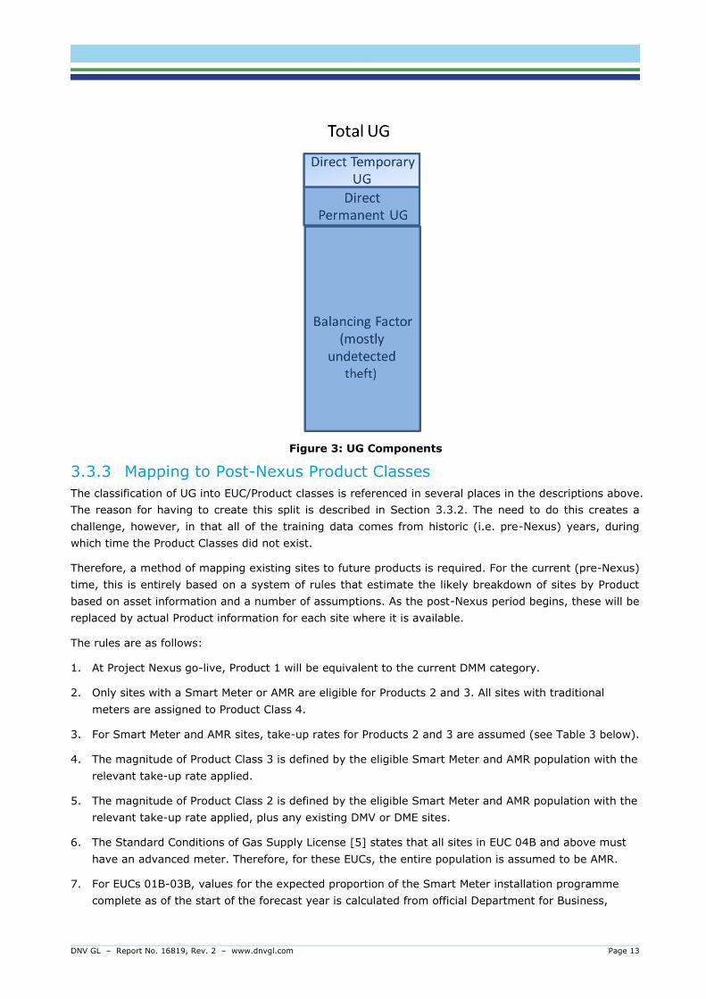
DNV GL – Report No. 16819, Rev. 2 – www.dnvgl.com Page 13
Figure 3: UG Components
3.3.3 Mapping to Post-Nexus Product Classes
The classification of UG into EUC/Product classes is referenced in several places in the descriptions above.
The reason for having to create this split is described in Section 3.3.2. The need to do this creates a
challenge, however, in that all of the training data comes from historic (i.e. pre-Nexus) years, during
which time the Product Classes did not exist.
Therefore, a method of mapping existing sites to future products is required. For the current (pre-Nexus)
time, this is entirely based on a system of rules that estimate the likely breakdown of sites by Product
based on asset information and a number of assumptions. As the post-Nexus period begins, these will be
replaced by actual Product information for each site where it is available.
The rules are as follows:
1. At Project Nexus go-live, Product 1 will be equivalent to the current DMM category.
2. Only sites with a Smart Meter or AMR are eligible for Products 2 and 3. All sites with traditional
meters are assigned to Product Class 4.
3. For Smart Meter and AMR sites, take-up rates for Products 2 and 3 are assumed (see Table 3 below).
4. The magnitude of Product Class 3 is defined by the eligible Smart Meter and AMR population with the
relevant take-up rate applied.
5. The magnitude of Product Class 2 is defined by the eligible Smart Meter and AMR population with the
relevant take-up rate applied, plus any existing DMV or DME sites.
6. The Standard Conditions of Gas Supply License [5] states that all sites in EUC 04B and above must
have an advanced meter. Therefore, for these EUCs, the entire population is assumed to be AMR.
7. For EUCs 01B-03B, values for the expected proportion of the Smart Meter installation programme
complete as of the start of the forecast year is calculated from official Department for Business,
DNV GL – Report No. 16819, Rev. 2 – www.dnvgl.com Page 14
Energy and Industrial Strategy figures [17]. These can be seen in Table 3 below. These proportions
of 01B-03B sites are assumed to have Smart Meters.
8. For EUCs 02B and 03B, the existence of AMR is defined according to existing records.
These rules allow the existing meter population and market sector definition, and the UG that arises from
them, to be mapped onto Project Nexus Product Classes.
Values for the key parameters listed below must be estimated in order to allow these rules to be applied.
The values applied to each one, which are used throughout this analysis, are shown in Table 3. The take
up rates for Products 2 and 3 are derived from the volumetric assumptions used by Xoserve and
presented to the Project Nexus workgroup [15]. Xoserve suggested around 75% of smart meter sites
with AQ < 732,000 kWh will remain in Product Class 4. The remaining 25% have been split between
Product Classes 2 and 3.
Note that there is no assumption that all Smart Meter sites are precluded from being in Product Class 4:
whilst the CMA Gas Settlement remedies document [6] requires Smart Meter reads to be submitted
monthly it does not require the readings themselves to be daily, and hence such sites are still eligible for
Product Class 4. This is currently being reviewed under UNC Modification 0594R [11].
Parameter Value
Smart Meter Installation Programme Completion (start of forecast year): EUC 01B 16%
Smart Meter Installation Programme Completion (start of forecast year): EUCs 02B-03B 13%
Product 2 Take Up (for Smart Meter and AMR Sites) 10%
Product 3 Take Up (for Smart Meter and AMR Sites) 15%
Table 3: Product Class Assignment Key Parameters
3.3.4 Projection of Permanent UG to Forecast Period
Having calculated the best estimates of Permanent and Temporary UG for each historic year for which
reliable data is available (the training period), it is then necessary to calculate the projected values of
Permanent UG for the forecast year (see Figure 4). Note that the estimated values for the forecast year
are calculated based on seasonal normal weather. The projection is carried out individually for each UG
component category and EUC/Product class, in each case using the most suitable data and extrapolation
technique. Extrapolation to the forecast period is carried out for each of:
Shipperless and Unregistered
iGT CSEPs
SSP and LSP Metering Errors
Balancing Factor
The methods used differ based on the observed behaviour of each category of UG, and are in many
cases affected by a number of UNC modifications introduced in order to address various UG issues. The
Balancing Factor is calculated for each of the six historic years with reliable meter read data (2009/10 to
2014/15) and projected forward based on the pattern observed in this time period. Input data for the

DNV GL – Report No. 16819, Rev. 2 – www.dnvgl.com Page 15
directly estimated components of UG is reliable throughout and so all available data is used. Properties
of the Balancing Factor and full details of the extrapolation techniques used in all cases are described
further in Section 6.
Balancing factor
Directly estimated
UG
Balancing factor
Directly estimated
UG
Balancing factor
Directly estimated
UG
Forecast
balancing factor
Directly estimated
UG
Balancing Factor:
Projection based on
pattern observed in
historic years
Direct UG:
Projection
based on
recent data
...
Figure 4: Projecting UG
As part of the estimation of the directly calculated UG components for the training years, an estimate of
the amount of Temporary UG for each component is made as described above. The values projected
forward to the forecast year are the permanent part of the UG only, however, for each EUC/Product
combination. Note that detected theft (up to 3-4 year cut-off date) is treated as a directly measured
component of UG (100% Temporary and hence not taken forward to the forecast year).
3.3.5 Unidentified Gas Factors
The final output of the UG analysis is a set of UG factors rather than direct estimates of the magnitude of
UG itself. These factors can be applied to the population (defined in terms of the aggregate AQ for each
EUC/Product) to give the relative magnitude of UG from each: these relative figures can then be applied
to the independent daily UG estimate that is made post-Nexus to give the final UG breakdown (in energy
terms) by EUC and Product Class.
The advantage of this approach is that this allows the effect of changing population to be taken account
of in the UG split without the need for the factors to change: when the number (and hence AQ) of sites
for a particular EUC/Product category goes up or down, the fact that this AQ is then multiplied by the
relevant UG factor ensures that the value of UG from this source also goes up or down accordingly. This
means that fixed factors can be generated that last a full year, until the results of the subsequent AUGE
analysis become available, with the effects of changing population during that year still taken into
account.
The factors themselves are a fundamental link between population and the UG from it, however, and so
they must be calculated using the detailed estimates of the value of UG (for the year in which the factors
will be in force) described above. Once the UG for each EUC/Product combination for the forecast year

DNV GL – Report No. 16819, Rev. 2 – www.dnvgl.com Page 16
has been estimated, this is converted into a factor by dividing by the relevant aggregate AQ (i.e. the
best estimate of the AQ for that EUC/Product combination for the forecast year):
UG FactorPRODUCT,EUC = UG (GWh)PRODUCT,EUC / Aggregate AQ (TWh)PRODUCT,EUC (3.3)
Note that the UG and Aggregate AQ have different units. This ensures that the resulting factors give
sufficient precision when expressed to 2 decimal places as required.

DNV GL – Report No. 16819, Rev. 2 – www.dnvgl.com Page 17
4 SUMMARY OF ANALYSIS
For future versions of the AUG Statement, this section will contain details of analyses carried out and
updates made to the UG calculation methodology since the last published document.
DNV GL – Report No. 16819, Rev. 2 – www.dnvgl.com Page 18
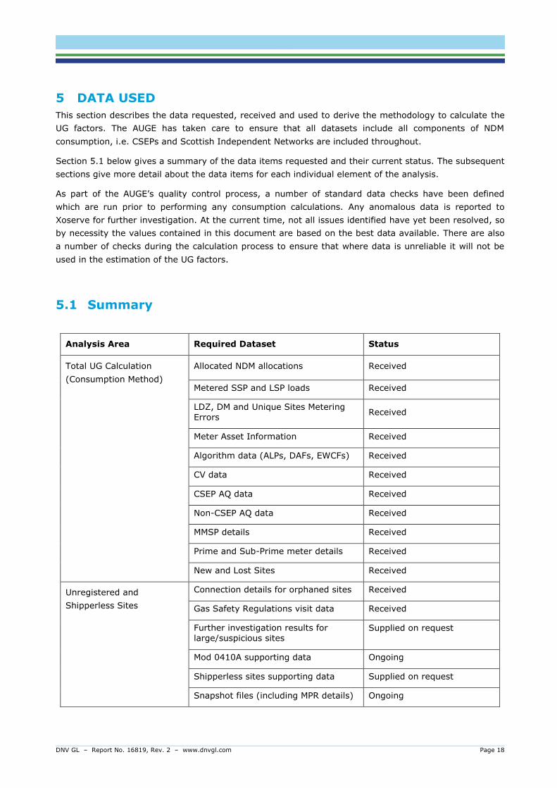
5 DATA USED
This section describes the data requested, received and used to derive the methodology to calculate the
UG factors. The AUGE has taken care to ensure that all datasets include all components of NDM
consumption, i.e. CSEPs and Scottish Independent Networks are included throughout.
Section 5.1 below gives a summary of the data items requested and their current status. The subsequent
sections give more detail about the data items for each individual element of the analysis.
As part of the AUGE’s quality control process, a number of standard data checks have been defined
which are run prior to performing any consumption calculations. Any anomalous data is reported to
Xoserve for further investigation. At the current time, not all issues identified have yet been resolved, so
by necessity the values contained in this document are based on the best data available. There are also
a number of checks during the calculation process to ensure that where data is unreliable it will not be
used in the estimation of the UG factors.
5.1 Summary
Analysis Area Required Dataset Status
Total UG Calculation
(Consumption Method)
Allocated NDM allocations Received
Metered SSP and LSP loads Received
LDZ, DM and Unique Sites Metering
Errors Received
Meter Asset Information Received
Algorithm data (ALPs, DAFs, EWCFs) Received
CV data Received
CSEP AQ data Received
Non-CSEP AQ data Received
MMSP details Received
Prime and Sub-Prime meter details Received
New and Lost Sites Received
Unregistered and
Shipperless Sites
Connection details for orphaned sites Received
Gas Safety Regulations visit data Received
Further investigation results for
large/suspicious sites Supplied on request
Mod 0410A supporting data Ongoing
Shipperless sites supporting data Supplied on request
Snapshot files (including MPR details) Ongoing
DNV GL – Report No. 16819, Rev. 2 – www.dnvgl.com Page 19
Analysis Area Required Dataset Status
iGT CSEPs Known CSEP data Received
Snapshot files Ongoing
Meter Error Meter capacity report Received
Theft Detected and alleged theft updated to
end June 2016 Received
Table 4: Data Status Summary
5.2 Total UG Calculation (Consumption Method)
Data has been requested from Xoserve in the following formats. In all cases, data has been provided for
gas years 2008/09 to 2014/15 with partial data for 2015/16.
Allocation data on a day-by-day basis, split by End User Category (EUC). This data includes CSEP
allocations.
Meter read data on an MPRN-by-MPRN basis, with one record for each meter read. Therefore, the
volume of data supplied for each MPRN is dependent on the meter read frequency for that meter.
Aggregate meter error adjustments for LDZs, DMs and Unique Sites.
Meter asset information on a MPRN-by-MPRN basis. This includes meter installation dates,
metric/imperial flag, numbers of meter dials, meter index units and T&P correction factors. This
information is used in several different parts of the consumption algorithm.
NDM Deeming Algorithm factors and CVs for the analysis period.
Aggregate MPRN count and AQ data by EUC for CSEPs. Meter read data is not available for these
sites, but knowledge of the number and AQ of MPRNs allows them to be included in the total UG
calculations when the sample consumption is scaled up to cover the full population.
A history of AQ and EUC data for each MPRN so that calculated consumptions can be validated
against AQs and failed meter points can be replaced with an appropriate EUC average.
Details of all meter points which have been part of a Multi-Meter Supply Point (MMSP) during the
analysis period.
Details of all meter points which are or have been part of a Prime and Sub configuration during the
analysis period. This includes re-confirmation data to track the potential disaggregation of prime and
sub configurations.
Lists of all new sites and lost sites during the analysis period, including start/end dates. These are
used to accurately track the population over time and to ensure that each new or lost site is only
included in calculations for the period for which it was active.
The provision of this data allows the consumption for each individual meter point, for each gas year of
interest, to be calculated using the method described in Section 6.2. The exact format of the data
provided is described in Appendix A.

DNV GL – Report No. 16819, Rev. 2 – www.dnvgl.com Page 20
5.3 IGT CSEP Setup and Registration Delays
Data for iGT CSEP setup and registration delays consists of two elements, as follows:
Unknown projects summary, including
the number of unknown projects by LDZ
a count of supply points and aggregate AQ of unknown projects by LDZ
This data is supplied by Xoserve in monthly snapshot files on an ongoing basis.
Known CSEP Data
This file contains data for both registered sites on known CSEPs and Unregistered sites on known
CSEPs. It is supplied on an annual basis and contains the following data fields:
LDZ
EUC
Number of supply points
Aggregate AQ
5.4 Unregistered/Shipperless Sites
The following information is supplied by Xoserve for all Unregistered and Shipperless sites (data supplied
on a site by site basis). Xoserve have created a regular report to ensure that new data is collated and
sent to the AUGE every month. This report covers the following categories of Unregistered and
Shipperless sites:
Shipper Activity
These are new sites created more than 12 months previously, that a Shipper has declared an
interest in (such as by creating the MPRN), but are nevertheless not registered to any Shipper. This
data is split into sites believed to have a meter and those believed to have no meter.
Orphaned
These are new sites created more than 12 months previously, that no Shipper is currently declaring
an interest in. This data is split into sites believed to have a meter and those believed to have no
meter.
Shipperless Sites PTS (Passed to Shipper)
These are sites where a meter is listed as having been removed and 12 months later the gas
transporter visits the site to remove or make the service secure (the GSR visit), but finds a meter
connected to the service and capable of flowing gas. If it is the same meter as supposedly removed
12 months previously it is passed to the Shipper concerned to resolve.
Shipperless Sites SSrP (Shipper Specific Report)
Similar to Shipperless (Passed to Shipper) sites, these are sites where the GSR visit finds a new
meter fitted and capable of flowing gas, in which case it is reported to all Shippers.
DNV GL – Report No. 16819, Rev. 2 – www.dnvgl.com Page 21
No Activity
These are sites currently being processed. They will end up in one of the other categories.
Legitimately Unregistered
These are sites believed to have no meter and hence are not capable of flowing gas.
Unregistered <12 Months
These are new sites that have been in existence less than 12 months and are not registered with a
Shipper. Action is not taken on such sites until they have been in existence for 12 months. At this
point they will move to either the Shipper Activity or the Orphaned category.
For all of these Unregistered/Shipperless UG categories, the following information is supplied for each
site:
Dummy MPRN
LDZ
AQ
Meter Point Status
In addition, the following data is supplied for individual UG categories:
Meter Attached Y/N
o Shipper Activity, Orphaned, No Activity, Legitimate
Meter Point Effective Date
o Shipper Activity, Orphaned, Unregistered <12 Months, No Activity, Legitimate
Shipperless Date
o Shipperless PTS, Shipperless SSrP
Isolation Date
o Shipperless PTS, Shipperless SSrP
In addition, the following information is supplied on an annual basis:
A summary of the remaining Shipperless sites, i.e. those that have been recorded as Isolated for less
than 12 months and are awaiting their GSR visit. These sites do not yet appear in the Shipperless
PTS or Shipperless SSP lists because sites only qualify for these after the GSR visit has found a
meter at the site. This data comes from GSR visit records.
Connection details for Orphaned sites, including asset and Shipper meter reads and information on
whether the confirming Shipper is the same as the Shipper whose Supplier requested asset
installation. This data is used to determine the proportion of sites that have been flowing gas prior to
becoming registered and the proportion of these that can be back-billed.
Shipperless sites supporting data. This is used to ascertain the final outcome for each Shipperless
site that has appeared in any snapshot but has subsequently been either disconnected or

DNV GL – Report No. 16819, Rev. 2 – www.dnvgl.com Page 22
(re)confirmed. This is used to determine whether the UG arising from them is temporary or
permanent under the terms of Mods 0424 [7] and 0425 [8].
5.5 Meter Errors
Data for meter error calculations consists of meter capacity, AQ and LDZ for all commercial sites. This
report is supplied on an annual basis, with the latest one having been received by the AUGE in August
2016. This data is used to identify sites that due to the combination of AQ and meter capacity are likely
to be operating at either a high or low extreme of their range, where bias in the readings starts to occur.
5.6 Theft
This data consists of all recorded detected and alleged thefts from 2008 to June 2016. For each theft,
the following key data items are supplied:
Dummy MPRN
Theft start and end dates
LDZ
Meter AQ
Estimate of energy value of theft (kWh)
5.7 Shrinkage
There are two elements of Shrinkage that affect the UG calculation, and the data used in the
quantification of each one is described below:
Shrinkage Error
o Total LDZ shrinkage from each training year (from Gas Transporters annual shrinkage
reports [19])
o Estimated bias in Shrinkage estimate (from GRG study [16])
CSEP Shrinkage
o Total LDZ shrinkage from each training year (from Gas Transporters annual shrinkage
reports [19])
o Estimated bias in Shrinkage estimate (from GRG study [16])
o CSEP composition (AQ by EUC/Product Class)

DNV GL – Report No. 16819, Rev. 2 – www.dnvgl.com Page 23
6 METHODOLOGY
This section describes in detail the methodology for estimating each element of Unidentified Gas.
The first stage in the calculation process is to use the Consumption Method to estimate the total UG for
each year in the training period. This process is very similar to that used by the AUGE previously [10]
but has been updated to account for the change in definition of the AUG year to align with the gas year
following implementation of Mod 0572 [12]. The method has also been updated to allow for the
disaggregation of meter points in a prime/sub configuration.
All directly estimated UG categories are then calculated for the same period: this allows the amount of
Temporary UG within the Consumption Method total for each year to be ascertained, and also allows the
Balancing Factor (mostly undetected theft) to be calculated. All UG in the Balancing Factor is Permanent.
The data patterns observed in the training period for each UG component, including the Balancing Factor,
are used to extrapolate to the forecast year (currently 2017/18) and provide the best estimate of each
Permanent element of UG for this year. This is carried out individually for all 36 EUC/Product
combinations for every UG category. Finally, these UG estimates are converted into factors by dividing
by the GWh UG estimates for the forecast year by the aggregate AQ for each EUC/Product combination,
as per equation 3.3 in Section 3.3.5.
As given in equation 3.2 (Section 3.3.1), the Consumption Method can be stated in its simplest form as:
Total UG = NDM Allocation - Metered NDM Consumption
This calculation involves correcting the allocations to take account of meter errors (LDZ offtake and DM)
and calculating the metered consumption using meter reads, metered volumes or an EUC average
consumption for sites where no reliable metered data is available.
The Total UG calculated as above includes both Permanent and Temporary Unidentified Gas. Therefore,
Temporary UG (calculated from the individual component parts of UG) has to be subtracted from the
initial UG total, and it is this amended figure that then goes forward into the remainder of the
calculations.
6.1 Correcting the NDM Allocation
The NDM allocation is calculated as
AllocNDM = Aggregate LDZ Load – DM Load – Shrinkage
Any subsequently detected significant errors in these three components will constitute Temporary UG
which has since been reconciled. Therefore, the allocations are corrected to remove this element.
6.1.1 Known DM and LDZ Metering Errors
Meter error adjustment data is received on an LDZ by LDZ basis split by billing month. The total value of
the error is given, and this is split so that the correct proportion of each meter error can be assigned to
each gas year in which the error occurred.
These errors affect the Aggregate LDZ Load and the DM Load, and have opposite effects on the
allocation total, which is calculated at the gas year level of granularity. The result of applying corrections
for the meter errors is as follows:
LDZ meter under-reads increase the total NDM allocation
LDZ meter over-reads decrease the total NDM allocation

DNV GL – Report No. 16819, Rev. 2 – www.dnvgl.com Page 24
DM/Unique site meter under-reads decrease the total NDM allocation
DM/Unique site meter over-reads increase the total NDM allocation
6.1.2 Shrinkage Error
Whilst Shrinkage error is not strictly a component of UG, bias in the Shrinkage estimate does affect the
UG calculation:
If Shrinkage is consistently under-estimated, this will inflate the UG figure.
In this circumstance, the additional amount of gas introduced to the estimate is actually
unaccounted-for Shrinkage rather than UG and hence it should not be dealt with through the UG
process in the long term. For the short term, however, it is recognised that until the bias in the
Shrinkage model is dealt with this gas will not be accounted for anywhere else and hence the best
interim solution is for UG to pick it up. As stated previously, unless specific steps are taken to include
Shrinkage error in the directly-estimated elements of UG it will feed through into the Balancing
Factor. Shrinkage error needs to be split by throughput, however, whilst the Balancing Factor is split
by the relative level of theft, and the inclusion of Shrinkage error in the Balancing Factor will
invalidate the assumption that it is largely composed of undetected theft. Therefore the Shrinkage
Error is estimated directly and split by throughput (all EUCs and Product Classes), hence removing
this element from the Balancing Factor.
If Shrinkage is consistently over-estimated, this will reduce the UG figure.
In this circumstance the over-estimation of Shrinkage will result in the opposite effect, i.e. that some
gas that is really UG is instead contained in the Shrinkage calculation. The long-term solution to this
is once again for the bias in the Shrinkage models to be addressed. In the meantime, the UG
estimates will be left unchanged to avoid introducing error into the Unidentified Gas process as well
as Shrinkage.
It should be noted that the current best estimate of Shrinkage error, as contained in the GRG report [16],
is an under-estimate of 20%. This will therefore be addressed as a directly-estimated element of UG, as
described in Section 6.7 below.
6.2 NDM Consumption Calculation
The consumption algorithm relies on a large quantity of data, summarised in Section 5.2. A full
description of the raw data used to calculate consumption figures for each individual meter point is
described in Appendix A. This raw data is then pre-processed to validate it and to derive additional
information to help speed up the consumption calculation process. After the pre-processing the main
algorithm is run to calculate consumption on a meter by meter basis. This calculation will not be
successful in all cases so a final step is required to scale up the consumption estimate to account for
these ‘failed’ sites.
6.2.1 Algorithm
Figure 5 shows a flow chart of the process involved to calculate the consumption for a single meter and
gas year with references to numbered steps, which are described in detail below.
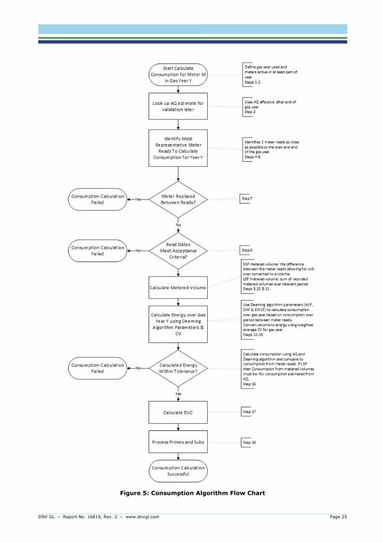
DNV GL – Report No. 16819, Rev. 2 – www.dnvgl.com Page 25
Figure 5: Consumption Algorithm Flow Chart

DNV GL – Report No. 16819, Rev. 2 – www.dnvgl.com Page 26
1. Given a gas year Y, define the start and end dates as 01 Oct Y and 30 Sep Y+1
2. Find all meter points that were active and NDM in a least part of year Y.
3. Look up the first AQ estimate effective after the end of the gas year. If none exists after the end of
the gas year use the latest value. From this record store
i. The AQ value
ii. The EUC provided by Xoserve
iii. The pre-calculated consumption band derived by the AUGE from the AQ value.
iv. Market sector (SSP/LSP) based on the EUC from Xoserve
4. For each meter point find the meter reading date and value for:
LB1 (Lower Bound 1) – the latest meter reading prior to the start of the gas year
LB2 (Lower Bound 2) – the earliest meter reading within the gas year
UB1 (Upper Bound 1) – the latest meter reading within the gas year
UB2 (Upper Bound 2) – the earliest meter reading after the end of the gas year
For SSPs those readings which have been flagged as bad by the pre-processing are excluded.
Where a meter point has changed between NDM and DM or vice versa try to select meter reads from
the period when it was NDM.
Note that for any given meter point, only a subset of this full set of reads may be available. At least
one lower bound and one different upper bound meter read are needed. Possible scenarios are
shown in Figure 6 below:

DNV GL – Report No. 16819, Rev. 2 – www.dnvgl.com Page 27
Figure 6: Meter Read Availability Scenarios
5. Set the start meter read date to LB1 unless
A. the date of LB1 is more than 540 days from the start of the gas year, or
B. the meter was replaced on or after LB1 and before LB2
In which case set it equal to LB2.
6. Set the end meter read date to UB2 unless

DNV GL – Report No. 16819, Rev. 2 – www.dnvgl.com Page 28
A. the date of UB2 is more than 540 days from the end of the gas year, or
B. the meter was replaced after UB1 and on or before UB2
In which case set it equal to UB1.
7. If the meter was replaced between LB2 and UB1 inclusive, then reject the meter point.
8. Check that:
A. The distance between the two chosen meter readings is at least 120 days
B. The overlap between the metering period and the gas year is at least 60 days
If this is true then proceed to calculating the metered volume, otherwise reject the meter point.
9. Apply either Rule A or Rule B according to the market sector of the meter point:
A. If the site is SSP then calculate the volume consumed between the two chosen meter
readings (mr1, mr2). If this gives a negative volume, then check if the meter index has rolled
over (see subsection below).
B. Otherwise sum the metered volumes (mvi) and volume corrections between the two chosen
meter readings. If there are any negative volumes in the range, set the sum to -1.
If this step produces a positive volume then proceed to the next step, otherwise reject the meter
point.
10. Calculate the fraction of the year that the meter point was active and NDM weighted by the WAALPs.
11. Calculate the volume taken over the gas year (or fraction of year calculated in the previous step) by
multiplying the volume from Step 9 by
PeriodMetered
v
ThereofPartorYearFormula
v
WAALP
WAALP
where WAALPv is the WAALP divided by the relevant CV value (i.e. a ‘volume’ WAALP rather than the
usual energy WAALP).
12. Look up, in the meter asset information, whether the meter is/was metric or imperial and then apply
either Rule A or Rule B to match the rule chosen in step 9.
A. If the meter point is SSP look up the read units (U).
First choice is the units inferred from the meter read records.
If this could not be calculated, then use the units provided by Xoserve.
In the case where the read units from Xoserve are obviously wrong (i.e. are 0 or not a
power of 10) use 1 for metric and 100 for imperial meters.
Combine this value with the default correction factor (CF) 1.022640 and relevant
metric/imperial conversion factor to get a combined conversion factor.
B. Otherwise, if LSP look up the appropriate metric/imperial factor.

DNV GL – Report No. 16819, Rev. 2 – www.dnvgl.com Page 29
If no meter asset information can be found, reject the meter point.
13. Calculate the weighted average CV for the gas year, calculated as
ThereofPartorYearFormula
v
ThereofPartorYearFormula
WAALP
WAALP
14. Convert the gas year volume to energy in kWh by multiplying the output of Steps 11, 12 and 13
together. In summary, depending on the market sector of the meter point, this will be
imperialifCVCFUmrmrCon 0283168466.06.3/12 for SSP
imperialifCVmvCon i 0283168466.06.3/ for LSP
15. Calculate an AQ from this consumption using the appropriate Cumulative Weather Adjusted Annual
Load Profile (CWAALP)
AQ = Con * 365 / CWAALP
16. If a new AQ value has been calculated from the meter readings which is more than five times larger
than the old AQ and the new AQ puts the site in the LSP market, then reject the meter point. If the
old AQ is 1 then use five times the largest recorded AQ as the check instead.
17. If the consumption calculation was successful, calculate an EUC band based on the new AQ.
18. Carry out post-processing to avoid double counting of subs and deduct consumption. See subsection
below for details.
Meter Index Rollover Check
Given two reads mr1 and mr2 where (mr2 - mr1) < 0 the following process is used:
1. Estimate the number of dials from mr1
num_dials = max(ceil(log10(mr1)), 4)
2. Determine the maximum possible meter read
max_read = 10num_dials
3. Calculate the period between the two meter reads in years
365 / ALP(date)mr
1(date)mr
2
1
yearsnum _
4. Assume meter index roll-over and re-calculate the volume
tmp1 = max_read – mr1 + mr2
5. Calculate the new volume as a fraction of the max read per year
tmp2 = (tmp1 / max_read) / num_years

DNV GL – Report No. 16819, Rev. 2 – www.dnvgl.com Page 30
6. If tmp2 < 0.25 then assume the meter index has rolled over and use tmp1. Otherwise leave the
calculated volume as negative and reject the meter point.
Prime and Sub Meter Post Processing
As the prime meter consumption is the difference between the total consumption (based on the prime
meter reads) minus the sum of the sub-meter consumptions, issues can arise in cases where a full valid
set of consumptions for all meters within a sub-prime configuration are unavailable. Note that the
consumption methodology will not calculate consumption for a DM meter. There are four cases to
consider:
1. If the prime meter is DM, no action is necessary as the methodology won’t have calculated
consumption for the prime meter (consumption not required for DM meters). Sub-meters will be
calculated correctly based on available data.
2. If the prime meter is NDM and contains one or more DM sub-meters, then the prime meter
consumption calculation is flagged as having failed so that an EUC average consumption is used (see
6.2.2).
3. If the consumption calculation fails for any of the sub-meters, then the prime meter calculation is
flagged as having failed. An EUC average consumption is therefore used for the prime meter.
4. If the consumption calculation succeeds for the prime meter and all of its sub-meters, then the prime
meter consumption is calculated by subtracting the sub-meter consumptions from the total prime
meter consumption.
Prime and sub meter arrangements may be disaggregated so data was requested from Xoserve to track
the reconfirmation of these meters. Using this information, the necessary correction is made only for the
relevant period.
6.2.2 Aggregation and Scaling-Up
When applied to each meter point in any given LDZ, the algorithm outputs a set of consumptions that
can be aggregated to EUC level. The aggregated data for each EUC is also naturally split into the
following categories by the algorithm:
Meters for which a consumption could be calculated
Meters for which the algorithm failed (failed to calculate consumption or calculated consumption
failed validation)
Meters in CSEPs (for which meter reads are not available)
The sum of these three categories across all EUCs gives the total NDM population of the LDZ.
Where a consumption value was successfully calculated the EUC is based on this consumption, otherwise
it is calculated by the AUGE based on the AQ.
Therefore, for each EUC band the following can be calculated:
1. The number of meter points with a successfully calculated consumption.
2. The number of meter points without a calculated consumption (i.e. calculation failed).

DNV GL – Report No. 16819, Rev. 2 – www.dnvgl.com Page 31
3. The average consumption for those meter points with a calculated consumption greater than zero.
The values for 3) are then used to estimate the consumption for meter points in 2). This involves a
number of subtleties:
In 3) attention is restricted to consuming meters only, in order to account for potential
differences in the proportion of non-consuming meters within and outside the sample.
Meter points where the consumption calculation fails are classified as consuming/non-consuming
based on AQ, as this is the only reliable data available for such meters. It is recognised that due
to changing circumstances for each meter, those with an AQ of 1 for Year X are not necessarily
non-consuming during Year X. Likewise, those with an AQ greater than 1 for Year X are not
necessarily consuming in Year X. Therefore, two figures have been calculated using available
information (i.e. meters within the sample):
o the proportion of meters with AQ = 1 for Year X that are consuming in Year X = A
o the proportion of meters with AQ > 1 for Year X that are consuming in Year X = B
The consumption for the non-calculated meter points is then calculated as
Consumption = A x (meters with AQ = 1) x “AQ=1” average consumption
+ B x (meters with AQ > 1) x EUC average consumption
Where:
“AQ=1” average consumption is the average consumption of meter points where the AQ=1,
but our consumption estimate is greater than zero. This can arise when an AQ review
produces AQ=1 yet the period of consumption being validated is actually non-zero.
EUC average consumption is the average consumption for successfully calculated meters in
the corresponding EUC Band. The 01B EUC average excludes meters where AQ=1.
CSEPs are treated differently to failed meters. This is because meter points are assigned to EUC
band based on their maximum potential AQ which may not be the same as their current AQ. It is
not appropriate to estimate their consumption using the number of meter points in each EUC
band multiplied by the EUC band average consumption. The approach used is described in detail
in Section 6.3.3.1.
Where the sample size for a particular EUC for a given LDZ and gas year is less than 30 the
national average is used in place of the LDZ average.
Failed meter points which were only active for part of the year are assigned an average demand
scaled based on the sum of WAALPs for that part of the year.
Figure 7 below summarises the process for obtaining a consumption value for each type of meter
point.

DNV GL – Report No. 16819, Rev. 2 – www.dnvgl.com Page 32
Figure 7: Consumption Method used for each type of Meter Point
UG for the LDZ for the gas year in question is then calculated by summing the metered NDM
consumptions across all EUCs and subtracting these from the total combined allocations for the same
period.
It is important to note that at this stage these figures still include Temporary UG. Therefore, whilst
giving an indication of the order of magnitude of the Permanent UG total for that historic year, this is
simply a step in the calculation process and not an estimate of the final value. The method for
calculating the remaining Temporary elements is defined in detail in the relevant subsections below.
6.2.2.1 CSEP Consumption Calculation
The following steps are used in the calculation of CSEP consumption for gas year Y. The steps are
carried out separately for each LDZ and EUC for each gas year. All references to AQ mean the CSEP AQ
for the corresponding LDZ and EUC unless stated otherwise.
In most cases, the snapshots of CSEP AQ and supply point count are provided at the start of each gas
year (1 Oct). However, the 2013 and 2014 snapshots provided are for February and it is not possible to
obtain historical snapshots aligned to the gas year.
1. If the number of meter points in the CSEP is less than 100 in year Y then the CSEP consumption
estimate for year Y is the aggregate AQ for year Y
Consuming Meters
Non-Consuming Meters
Non-Consuming Meters
Consuming Meters
Individual Meter Consumption
Calculations
Meters with
Consumption
Calculated
Successfully
Calculated
Consumption
Calculated
Consumption
= Zero
Meters where
Consumption
Calculation
Failed
Zero
Consumption
Consumption Used
CSEPs
Average EUC
Consumption
Based on AQs
DNV GL – Report No. 16819, Rev. 2 – www.dnvgl.com Page 33
CY = AQY
Otherwise,
2. Calculate the average AQ for new meters
For EUC01B before gas year 2012,
NMAQ = AQ2007 / N2007
For EUC01B for gas years 2012 and 2013,
NMAQ = AQ2012 / N2012
For all other EUCs and EUC01B from gas year 2014 onwards,
NMAQ = AQY+1 / NY+1
Prior to 2012, the CSEP NExA table had not been updated since 2007. A new table was
calculated for 2012 and this is now updated annually following iGT 053 which was implemented
from 1 October 2014 [13]. This removes the additional bias which previously existed for 01B
meters as a result of using default AQ values.
3. Calculate the average AQ for lost meters
LMAQ = AQY / NY
4. Estimate the aggregate AQ for year Y by adjusting Y+1 for meter changes
AQ’Y = AQY+1 - Max(0, (NY+1 - NY) * NMAQ) - Min(0, (NY+1 - NY) * LMAQ)
5. Adjust the aggregate AQ to allow for the recalculation success rate
AQ’’Y = AQY + (AQ’Y - AQY) / RR
where
AQY is aggregate AQ in year Y. Note that for 2009, AQY is adjusted to the new SNCWV definition.
AQ’Y is the aggregate AQ in year Y+1 adjusted to allow for the different number of meters to
year Y (as in step 4 above)
RR is the recalculation success rate expressed as a fraction
6. Estimate consumption for year Y by adding effect of new/lost meters
CY = AQ’’Y + Max(0, (NY+1 - NY) * MAQY+1) * YFrac + Min(0, (NY+1 - NY) * MAQY) * (1-YFrac)
where
CY is the final estimate of aggregate CSEP consumption for year Y
AQ’’Y is the estimate of aggregate AQ for year Y calculated from year Y+1 and adjusted for the
recalculation success rate
NY is the number of meters in year Y
MAQY is the average AQ per meter in year Y and is calculated as AQY / NY
YFrac is an estimate of the proportion of a year’s consumption which new meters contribute. It is
assumed that new and lost meters will be consuming on average for half of the year so a default
DNV GL – Report No. 16819, Rev. 2 – www.dnvgl.com Page 34
factor of 0.5 is used. However, as not all snapshots are based on 1 October, a further
adjustment is applied to allow for snapshots which aren’t exactly one year apart. This only
affects gas years 2012 and 2014. For example, the 2014 snapshot was provided for February
2014 whilst the 2015 snapshot was for October 2015. This is a period of 20 months rather than
12. In this instance the default factor of 0.5 will be adjusted to be 0.5*12/20.
If the consumption estimate is negative, then use the AQ as the best estimate of consumption i.e. CY =
AQY.
6.3 Unregistered and Shipperless Sites
The magnitude of every Unregistered and Shipperless category of Unidentified Gas is affected by a
number of Mods introduced between 2013 and 2014 to address and reduce these specific areas of UG.
The Mods in question are as follows:
Mod 0410A [9] applies to Shipper Activity, Orphaned and Unregistered <12 Months, and any site
created on or after 01/09/2013 is subject to the terms of this Mod.
Mod 0424 [7] applies to Shipperless PTS, and any site with an isolation date on or after 01/04/2013
is subject to the terms of this Mod. This results in all UG from post-Mod sites being Temporary rather
than Permanent.
Mod 0425 [8] applies to Shipperless PTS, and any site with an isolation date on or after 01/04/2014
is subject to the terms of this Mod. In theory, this should have resulted in all UG from post-Mod sites
being temporary rather than Permanent but the process required to implement this is not available
in the pre-Nexus system. Therefore, all UG from post-Mod sites will only become Temporary after
the implementation of Project Nexus (i.e. for the forecast year but not the training years).
Note that Mods 0424 and 0425 apply to the PTS and SSrP elements of the “Awaiting GSR Visit” category
in addition to their main categories.
A full description of the calculation method for all Unregistered and Shipperless UG categories is given
below. Raw data for all of these except “Awaiting GSR Visit” is contained in snapshot files supplied by
Xoserve every month. These are described in Section 5.4 above.
The following files also contain data that is used in the calculation process and are supplied on an annual
basis.
Connection Details for Orphaned Sites
This dataset includes asset and Shipper meter reads and information on whether the confirming
Shipper is the same as the asset Shipper. This data is used to determine the proportion of sites that
have been flowing gas prior to becoming registered and the proportion of these that can be back-
billed. Backbilling can only occur if the confirming Shipper is the same as the Shipper that carried out
site works. The Connection Details dataset is split into two categories (pre-Mod 0410A sites and
post-Mod 0410A sites) and different flow proportions and backbilling proportions are calculated for
each. This is necessary because the terms of Mod 0410A affect how Unregistered sites are processed,
and this leads to different conditions for pre-Mod and post-Mod sites.
Gas Safety Regulations Visit Details
The gas safety visit data is used to estimate the number and AQ of sites that have been recorded as
isolated for less than 12 months and hence have not yet had their GSR visit and do not yet appear in
the snapshots as Shipperless PTS or Shipperless SSrP, but are nevertheless still consuming
Shipperless gas.

DNV GL – Report No. 16819, Rev. 2 – www.dnvgl.com Page 35
Shipperless Sites Supporting Data
This dataset contains the confirmation date of each Shipperless site that has appeared in any
snapshot but has subsequently been (re)confirmed. It is used to ascertain the final outcome for each
of the sites, i.e. whether it was (re)confirmed or whether it was disconnected. This is used to
determine the proportion of Shipperless sites that have a meter and are capable of flowing gas that
actually are flowing gas.
Further details of these data files are also given in Section 5.4 above.
The step by step calculation process for Shipperless and Unregistered UG is as follows:
1. Each MPRN in the snapshot files is assessed and flagged for further investigation by Xoserve if any of
the conditions specified below are satisfied.
If a graph of AQs sorted by descending magnitude contains a “shoulder” point (i.e. a distinct
change in gradient), any points to the left of the shoulder are flagged.
Any site with an AQ more than 100 times the average AQ for EUCs 02B-09B is flagged.
Any site with an AQ greater than 58.6 GWh is flagged.
The resultant list of flagged sites is sent to Xoserve.
2. Xoserve respond with details where any of the flagged sites have been confirmed on their system,
and the confirmed AQ of each such site is provided. Any differences between the queried AQs and
the confirmed AQs are applied to the snapshot files. Sites where Xoserve have no further information
are left as is.
3. All sites with a listed AQ above the VLDMC threshold (1.465 TWh) have their AQs replaced with the
average EUC 02B-09B AQ. VLDMCs cannot be Unregistered or Shipperless due to the greater
scrutiny the network code requires on such sites, and hence any AQ above this threshold in the
Unregistered or Shipperless lists must be erroneous (e.g. MPRN or phone number accidentally
entered in AQ field).
4. Before the analysis is run, the following coefficients are also calculated using the latest available data:
Fraction of opening meter reads with gas flow for Unregistered sites (for the
Permanent/Temporary split for Unregistered UG categories, with different fractions for pre-
01/09/2013 and post-01/09/2013 sites).
Fraction of Unregistered UG not backbilled (for the Permanent/Temporary split for Unregistered
UG categories, with different fractions for pre-01/09/2013 and post-01/09/2013 sites).
Proportion of Shipperless sites being disconnected rather than re-registered.
5. “Fraction of opening meter reads with gas flow” is calculated using the “Connection Details for
Orphaned Sites” spreadsheet. This file contains a list of Orphaned meters and includes both their
asset meter reading and their opening Shipper meter reading. The number of meters with gas flow
(i.e. those where the reading has changed) is expressed as a proportion of the total number of
meters in the sample. The dataset is split into two sections - pre-Mod 0410A sites and post-Mod
0410A sites – and separate factors are calculated for each in order to account for changes introduced
in the Mod. The calculated proportions are applied to the AQs of each pre-Mod 0410A and post-Mod
0410A site with a meter in the snapshots, to give an estimate of the consumption from sites that are
actually flowing gas in the Unregistered UG calculations.
DNV GL – Report No. 16819, Rev. 2 – www.dnvgl.com Page 36
6. “Fraction of Unregistered UG not backbilled” is also calculated using the “Connection Details for
Orphaned Sites” spreadsheet. In addition to the meter readings, this file contains a flag that
indicates whether the asset Shipper is the same as the confirming Shipper. This flag is used to
calculate the proportion of sites with gas flow (as calculated in Step 5 above) that also have a
different Shipper. This is the proportion of Unregistered sites that cannot be backbilled and hence
contribute permanent UG. As for “Fraction of opening meter reads with gas flow”, separate factors
are calculated for pre-Mod 0410A and post-Mod 0410A sites.
7. The proportion of Shipperless sites that are disconnected rather than reconfirmed is calculated using
information from the “Shipperless Sites Supporting Data” spreadsheet. Any site that disappears from
the Shipperless lists without appearing in the “Confirmed” list in the supporting data has been
disconnected and this is used to calculate the proportion that are disconnected rather than being
reconfirmed. This figure is used as the best estimate of the proportion of sites capable of flowing gas
that actually are flowing gas (i.e. it is assumed that if a site is flowing gas it is reconfirmed, and if it
is not it is disconnected).
8. The raw Shipperless/Unregistered UG calculations are now carried out. This is carried out in a series
of spreadsheets, with a set of spreadsheets for each individual UG category. Each of these sheets
contains a full history of all available snapshot data for the relevant UG category, which at present
runs from September 2011 to September 2016. The availability of snapshot data over such a period
of time means that trends can be identified within each UG category and extrapolated to cover
training years and the forecast year as necessary.
9. Every Shipperless and Unregistered category is affected by at least one Mod, and the implementation
of each of these Mods therefore affects the magnitude and trend of the UG category it refers to. In
addition, once the Mod has been implemented this creates a division of each category into pre-Mod
and post-Mod sites: only post-Mod sites are affected by the Mod, and hence pre- and post- sites will
now behave in different ways and exhibit different trends over time. Hence they must be analysed
separately. In addition, the rules for UG being temporary or permanent can be different before and
after the Mod and this must also be taken account of. This creates a set of four sub-categories of UG
for each main UG category as follows:
Pre-Mod permanent
Pre-Mod temporary
Post-Mod permanent
Post-Mod temporary
The trends for each of these must be assessed individually. For each one, the standard 36-way split
also exists (9 EUCs and 4 Product Classes), and it can also be seen from preliminary analysis of the
data that there is an LDZ-by-LDZ effect where different LDZs can show different patterns in UG
consumption. This creates a total of 1872 individual sub-categories for every main UG category (pre-
or post-Mod/permanent or temporary/LDZ/EUC/Product).
The trend for each of these must be individually assessed in order to allow accurate calculation of UG
for any time period covered by the snapshots, and accurate extrapolation to any required years that
fall outside this range (e.g. the forecast year).
Finally, the introduction of each Mod and the reaction of the industry to it necessarily affects these
trends, which will therefore not remain constant over the entire time period covered by the
snapshots. Therefore, for each main UG category, the snapshot period is split into a small number of
separate sub-periods where the trend is consistent: these differ for each UG category due to the
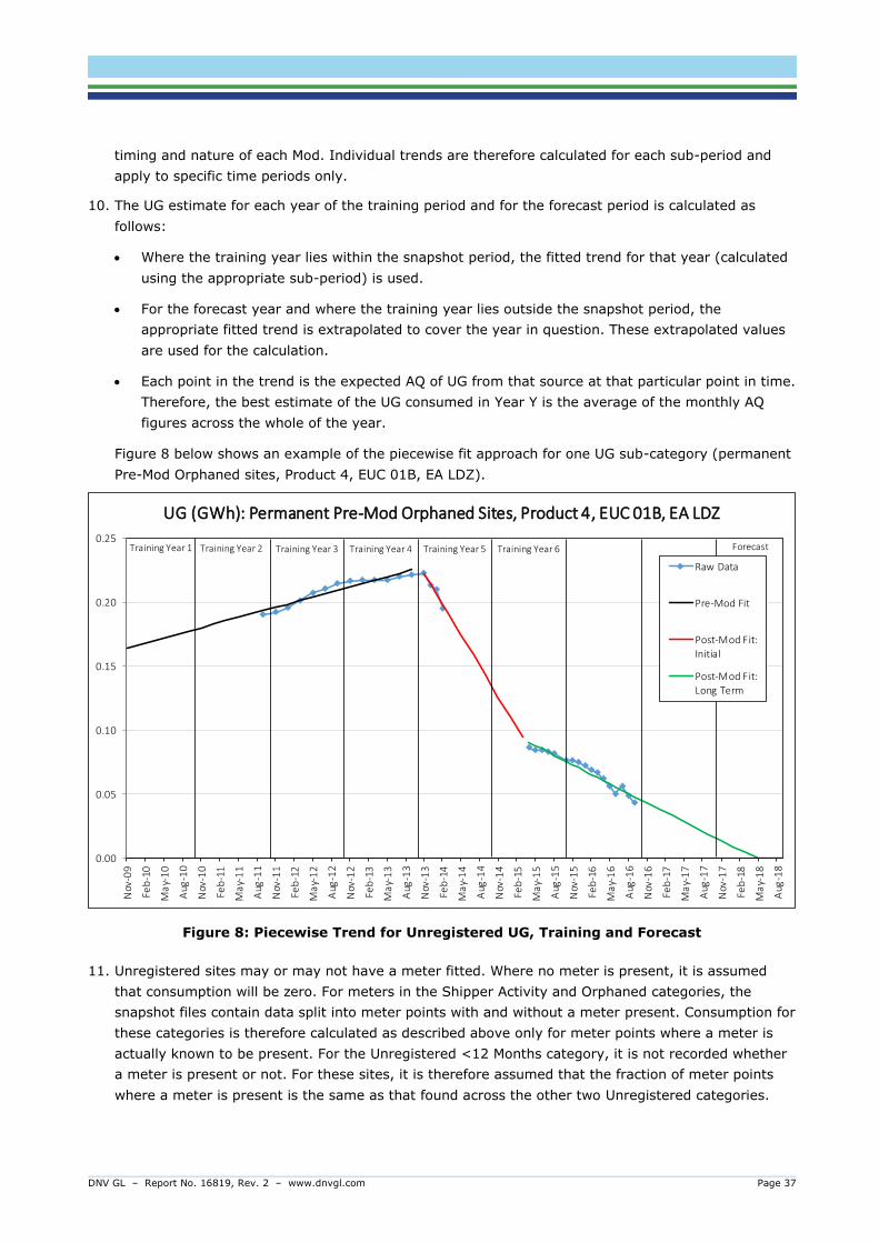
DNV GL – Report No. 16819, Rev. 2 – www.dnvgl.com Page 37
timing and nature of each Mod. Individual trends are therefore calculated for each sub-period and
apply to specific time periods only.
10. The UG estimate for each year of the training period and for the forecast period is calculated as
follows:
Where the training year lies within the snapshot period, the fitted trend for that year (calculated
using the appropriate sub-period) is used.
For the forecast year and where the training year lies outside the snapshot period, the
appropriate fitted trend is extrapolated to cover the year in question. These extrapolated values
are used for the calculation.
Each point in the trend is the expected AQ of UG from that source at that particular point in time.
Therefore, the best estimate of the UG consumed in Year Y is the average of the monthly AQ
figures across the whole of the year.
Figure 8 below shows an example of the piecewise fit approach for one UG sub-category (permanent
Pre-Mod Orphaned sites, Product 4, EUC 01B, EA LDZ).
Figure 8: Piecewise Trend for Unregistered UG, Training and Forecast
11. Unregistered sites may or may not have a meter fitted. Where no meter is present, it is assumed
that consumption will be zero. For meters in the Shipper Activity and Orphaned categories, the
snapshot files contain data split into meter points with and without a meter present. Consumption for
these categories is therefore calculated as described above only for meter points where a meter is
actually known to be present. For the Unregistered <12 Months category, it is not recorded whether
a meter is present or not. For these sites, it is therefore assumed that the fraction of meter points
where a meter is present is the same as that found across the other two Unregistered categories.
0.00
0.05
0.10
0.15
0.20
0.25
Nov
-09
Feb
-10
Ma
y-1
0
Aug
-10
Nov
-10
Feb
-11
Ma
y-1
1
Aug
-11
Nov
-11
Feb
-12
Ma
y-1
2
Aug
-12
Nov
-12
Feb
-13
Ma
y-1
3
Aug
-13
Nov
-13
Feb
-14
Ma
y-1
4
Aug
-14
Nov
-14
Feb
-15
Ma
y-1
5
Aug
-15
Nov
-15
Feb
-16
Ma
y-1
6
Aug
-16
Nov
-16
Feb
-17
Ma
y-1
7
Aug
-17
Nov
-17
Feb
-18
Ma
y-1
8
Aug
-18
UG (GWh): Permanent Pre-Mod Orphaned Sites, Product 4, EUC 01B, EA LDZ
Raw Data
Pre-Mod Fit
Post-Mod Fit:
Initial
Post-Mod Fit:
Long Term
Training Year 1 Training Year 2 Training Year 3 Training Year 4 Training Year 5 Training Year 6 Forecast

DNV GL – Report No. 16819, Rev. 2 – www.dnvgl.com Page 38
12. The UG estimate for each type of Unregistered site is adjusted to account for the proportion of such
sites with meters that actually flow gas whilst Unregistered, as described in Step 5 above. This
adjustment is applied to the annual UG values calculated from the piecewise trends described in Step
10.
13. For Shipperless sites, the snapshots contain all sites found to be capable of flowing gas at the GSR
visit. From these, the number actually flowing gas must be estimated. This is carried out using data
in the “Shipperless Sites Supporting Data” file supplied by Xoserve. This contains the confirmation
details of all sites that have appeared in the Shipperless report but have subsequently been
confirmed and is used to determine the proportion of sites that were reconfirmed rather than being
disconnected. The following assumptions are then made:
If the site was disconnected it was not flowing gas
If the site was reconfirmed it was flowing gas
The reconfirmation percentage is therefore applied to the Shipperless UG totals (calculated as
described in Step 10) to give the best estimate of the amount of Shipperless UG actually consumed.
14. For each Unregistered category, factors are used to convert from Requested AQ to Confirmed AQ and
then from Confirmed AQ to AQ Following Review, as follows:
Requested AQ Factor 1 Confirmed AQ Factor 2 AQ Following Review
The “AQ Following Review” figure is regarded as a reliable indicator of the annual consumption at the
site.
15. The UG estimates produced for each Shipperless/Unregistered category are multiplied by the
appropriate combination of these factors. This is carried out as follows:
Shipperless sites (PTS, SSrP): no adjustment required for AQ bias
Unregistered (Orphaned, Shipper Activity and Unregistered <12 Months): adjust using composite
Factor1(n) x Factor2, where n represents the UG category in question.
16. The above process allows UG estimates for all Unregistered and Shipperless UG categories apart
from “Awaiting GSR Visit” to be calculated. At the time of calculation these are split by:
UG Category
Permanent and temporary
Pre-Mod and Post-Mod
Year
EUC
Product Class
For use in further UG calculations, the estimates have to be split by permanent/temporary, Year,
EUC and Product Class and so figures are aggregated across categories and pre- or post-Mod status.
Tables of figures split this way feed into the final UG factor calculations.
17. “Awaiting GSR Visit” UG is calculated using Gas Safety Regulations visit data supplied by Xoserve.
This file contains the details of each Shipperless site that has crossed the 12-month threshold during
a period of a year and has subsequently been visited and found to be capable of flowing gas. The
actual sites listed in this file by definition appear in the summarised data in the snapshot files
because they have been Shipperless for more than 12 months. If it is assumed that sites become
DNV GL – Report No. 16819, Rev. 2 – www.dnvgl.com Page 39
Shipperless at a steady rate, however, it can be assumed that the number and AQ of sites crossing
the 12-month threshold in Year Y is a good approximation of the number and AQ that will cross in
Year Y+1. At the end of Year Y these sites will have been (recorded as) Isolated for less than 12
months and hence make up the “Awaiting GSR Visit” UG category for this year.
Therefore, in order to estimate the UG from this category, the AQs for each site from the GSR visit
data are analysed and split by:
Permanent and temporary
Year
EUC
Product Class
The transient nature of this UG category means that there is no requirement to define sites as pre-
Mod or post-Mod in this case. Whilst all sites in this category will go on to become either Shipperless
PTS or Shipperless SSrP sites and hence are affected by Mods 0424 and 0425 (subject to the delay
described above), all sites move on to their destination categories in a year and hence no legacy pre-
Mod sites remain.
The permanent/temporary split for each year is defined by the implementation date of the relevant
Mod, as follows:
For the PTS element, all UG from this source is permanent up to the 2011/12 gas year, and all
temporary from 2014/15 onwards. If a steady influx of sites is assumed for the remaining years,
this results in 75% of UG being permanent for 2012/13 and 25% permanent for 2013/14.
For the SSrP element, all UG from the pre-Nexus period is permanent due to the delay in
implementation of back-billing. Following Project Nexus go-live, any site without a record of the
installation date of the new meter will still contribute permanent UG until its GSR visit regardless
of the isolation date. It is assumed that new meters are installed at a steady rate for these sites
and as such the average period of the year for which a meter was present and capable of flowing
gas is 6 months (i.e. 50% of the year). The following calculation steps are applied:
Multiply the Shipperless SSrP UG element by the “% of Year with Meter” factor. This gives
the total (permanent plus Temporary) UG for the Shipperless SSrP element of “Awaiting GSR
Visit”.
Multiply this total by the “% of Meters without Install Date” factor. This gives the Permanent
element of the UG total from this source. The remainder of the UG for the Shipperless SSrP
element of “Awaiting GSR Visit” is Temporary.
Finally, the reconfirmation percentage (as described in Step 13 above) is applied to convert from the
AQ of sites capable of flowing gas to the AQ of sites actually flowing gas. This gives the final total UG
estimate for this category, split by permanent/temporary, Year, EUC and Product Class.
The UG from this category is now taken through into the final UG factor calculations.
DNV GL – Report No. 16819, Rev. 2 – www.dnvgl.com Page 40
6.4 IGT CSEPs
Connected System Exit Points (CSEPs) are typically small networks owned by Independent Gas
Transporters (iGTs) that connect to the GTs’ systems. They are often new housing estates, where the
gas network for the estate has been built and is owned by an iGT. CSEPs can potentially contribute to
Unidentified Gas where either sites within them or entire iGT networks are not recognised by the Xoserve
system and are thus consuming gas in an unrecorded manner.
6.4.1 Overview
UG from CSEPs arises from two sources: Unknown Projects and Unregistered sites on known CSEPs.
Unknown Projects are CSEPs that are known to exist but for various reasons are not on Xoserve’s
systems. Regular meetings are held between the iGTs and Xoserve in order to resolve these issues and
reduce the number of Unknown Projects.
Unregistered sites on known CSEPs lie in CSEPs that are on Xoserve systems, and Xoserve are notified of
such Unregistered sites on them.
For both these sources of UG from CSEPs, in the pre-Nexus market the UG from LSP sites is backbilled
and is hence temporary, whilst UG from SSP sites on CSEPs is not backbilled and is hence permanent.
Under Project Nexus, this translates to UG from EUC 01B being permanent, whilst that from other EUCs
is temporary.
It is necessary to calculate both the permanent and temporary elements of iGT CSEPs UG for the training
period, whilst only permanent is required for the forecast year. This allows temporary UG to be removed
from the raw UG total (permanent plus temporary) calculated using the Consumption Method for the
training period, leaving the final total as permanent UG only. Any permanent UG can then be
extrapolated to the forecast year to facilitate the calculation of the UG factors.
6.4.2 Data
Unknown Projects data is supplied by Xoserve in monthly snapshot files. These contain data for all
Unknown Projects, split by LDZ and by the year in which the CSEP first came to the attention of Xoserve.
For each LDZ, the total number of projects, the total number of supply points within them, and the sum
of their AQ is given. Note that no split between market sectors is given.
Unregistered sites on known CSEPs data is supplied in a file provided on an annual basis. This file
contains data for all known CSEPs, summarised to the LDZ and EUC level. For each EUC, the count of
supply points within CSEPs and their aggregate AQ is given. This is provided in separate tables for
registered sites and Unregistered sites.
Data for registered sites is used to calculate the average CSEP throughput percentages by EUC for each
LDZ, and this is used to split the Unknown Projects data by market sector.
Data for Unregistered sites is used to directly calculate the UG from this source for each LDZ.
It should be noted that the supply point count data for Unregistered sites is actually the number of times
Xoserve have been notified that the supply point is Unregistered rather than the number of sites that are
actually Unregistered. Xoserve are often notified about the same site on multiple occasions, and this
artificially inflates the supply point count figures in this dataset. Therefore, further analysis is carried out

DNV GL – Report No. 16819, Rev. 2 – www.dnvgl.com Page 41
on this data in order to estimate the actual number of Unregistered supply points. This is described in
more detail below.
6.4.3 Process
Processing is carried out in spreadsheets, which are supplied to the industry to allow auditing of the
AUGE’s calculations to take place. The following process steps are performed:
1. Data for registered sites on known CSEPs and Unregistered sites on known CSEPs is imported into
the calculation spreadsheets. The average AQ per site for each LDZ/EUC combination for registered
sites is calculated. As noted above, for the Unregistered data the number of notifications is recorded
rather than the number of sites, and hence the actual number of sites must be estimated.
2. The average AQ per site derived from the registered sites is used to estimate the number of
Unregistered sites in each EUC using the aggregate AQ for each EUC in the Unregistered dataset.
This gives an estimated number of Unregistered sites in each EUC under the assumption that each
site has the average AQ for that EUC.
If this calculated figure is lower than the number of notifications, it is used as the best estimate
of the number of Unregistered sites in that EUC.
If the number of notifications is lower, this is used as the best estimate of the number of
Unregistered sites in that EUC.
3. The total site count and aggregate AQ by EUC and by LDZ is calculated for registered sites. These
figures are then used to calculate the percentage split of CSEP site count by EUC and the percentage
split of CSEP AQ by EUC. This split is used in the calculations for Unknown Projects, described below.
4. The total site count and AQ by EUC and by LDZ is calculated for Unregistered sites. The AQ figures
produced are split by Product Class using the standard rules defined in Section 3.3.3 and are used
directly in the UG figures: these represent the estimated annual contribution to UG from
Unregistered sites in known CSEPs based on current conditions.
5. When each new monthly snapshot file becomes available, data for Unknown Projects is updated. The
snapshot tables are in the format shown in Table 5 below. In these tables, the “Year” field refers to
the year in which the CSEP came to the attention of Xoserve. For each LDZ the total number of
Unknown Projects, their aggregate AQ and the total number of supply points within them is given.
Each snapshot represents the situation at the point in time when it was produced.
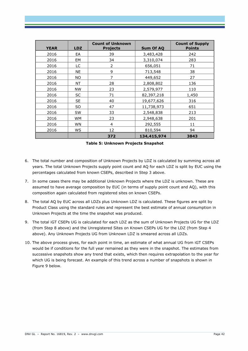
DNV GL – Report No. 16819, Rev. 2 – www.dnvgl.com Page 42
YEAR LDZ Count of Unknown
Projects Sum Of AQ Count of Supply
Points
2016 EA 39 3,483,428 242
2016 EM 34 3,310,074 283
2016 LC 2 656,051 71
2016 NE 9 713,548 38
2016 NO 7 449,652 27
2016 NT 28 2,808,802 136
2016 NW 23 2,579,977 110
2016 SC 71 82,397,218 1,450
2016 SE 40 19,677,626 316
2016 SO 47 11,738,973 651
2016 SW 33 2,548,838 213
2016 WM 23 2,948,638 201
2016 WN 4 292,555 11
2016 WS 12 810,594 94
372 134,415,974 3843
Table 5: Unknown Projects Snapshot
6. The total number and composition of Unknown Projects by LDZ is calculated by summing across all
years. The total Unknown Projects supply point count and AQ for each LDZ is split by EUC using the
percentages calculated from known CSEPs, described in Step 3 above.
7. In some cases there may be additional Unknown Projects where the LDZ is unknown. These are
assumed to have average composition by EUC (in terms of supply point count and AQ), with this
composition again calculated from registered sites on known CSEPs.
8. The total AQ by EUC across all LDZs plus Unknown LDZ is calculated. These figures are split by
Product Class using the standard rules and represent the best estimate of annual consumption in
Unknown Projects at the time the snapshot was produced.
9. The total iGT CSEPs UG is calculated for each LDZ as the sum of Unknown Projects UG for the LDZ
(from Step 8 above) and the Unregistered Sites on Known CSEPs UG for the LDZ (from Step 4
above). Any Unknown Projects UG from Unknown LDZ is smeared across all LDZs.
10. The above process gives, for each point in time, an estimate of what annual UG from iGT CSEPs
would be if conditions for the full year remained as they were in the snapshot. The estimates from
successive snapshots show any trend that exists, which then requires extrapolation to the year for
which UG is being forecast. An example of this trend across a number of snapshots is shown in
Figure 9 below.

DNV GL – Report No. 16819, Rev. 2 – www.dnvgl.com Page 43
Figure 9: iGT CSEPs UG by Snapshot
11. The above process leads to the creation of a total of 468 individual trend lines for UG from iGT CSEPs.
The identified snapshot-to-snapshot trend for each LDZ/Product Class/EUC combination is used to
extrapolate either forwards or backwards to each time period of interest. The UG for each year used
in the analysis is calculated using the fitted values for each snapshot date that falls within it. The
time periods in question cover the UG forecast year and the historic UG training years, with values
for each calculated using the fitted trend lines for each LDZ. The forecast year table is used directly
in the final UG factor calculations, whilst those for historic years are used in the calculation of total
UG and the Balancing Factor, which are based on data from the training years (currently 2009/10 to
2014/15).
12. For the pre-Nexus period, the UG calculated in this way from LSP sites is temporary. The UG
calculated in this way from SSP sites is permanent. In the post-Nexus world, Xoserve have
confirmed that all UG from this source will be reconcilable once the issue for the CSEP in question
has been resolved. Therefore, for the forecast period all iGT CSEPs UG is temporary and does not
form part of the permanent UG calculations.
6.5 Consumer Metering Errors
The effects of LDZ metering errors and known DM/Unique Site supply point errors are discussed in
Section 6.1.1 above. In addition, undetected errors in all consumer supply point meters can cause gas to
be burnt in an unrecorded or inaccurately recorded manner and hence have the potential to contribute to
Unidentified Gas. An assessment of this area of metering error has therefore been carried out by the
DNV GL Metering Team, and the conclusions drawn are presented here:
Very little work has been done in the field of accurately assessing meter drift over time. Information
is available about calibration curves taken at a particular point in time for certain meters, but there
has never been any dedicated work looking at how these change over time. Therefore, conclusions
drawn in this area are largely based on anecdotal evidence and/or extrapolation.
0.00
0.50
1.00
1.50
2.00
2.50
3.00
3.50
Jan
-15
Feb
-15
Ma
r-1
5
Apr
-15
Ma
y-1
5
Jun
-15
Jul-
15
Aug
-15
Sep
-15
Oct
-15
Nov
-15
De
c-1
5
Jan
-16
Feb
-16
Ma
r-1
6
Apr
-16
Ma
y-1
6
Jun
-16
iGT CSEPs UG (GWh): EM LDZ, Product 4, EUC 05B
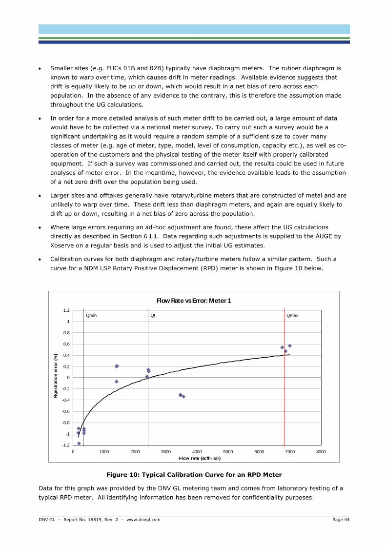
DNV GL – Report No. 16819, Rev. 2 – www.dnvgl.com Page 44
Smaller sites (e.g. EUCs 01B and 02B) typically have diaphragm meters. The rubber diaphragm is
known to warp over time, which causes drift in meter readings. Available evidence suggests that
drift is equally likely to be up or down, which would result in a net bias of zero across each
population. In the absence of any evidence to the contrary, this is therefore the assumption made
throughout the UG calculations.
In order for a more detailed analysis of such meter drift to be carried out, a large amount of data
would have to be collected via a national meter survey. To carry out such a survey would be a
significant undertaking as it would require a random sample of a sufficient size to cover many
classes of meter (e.g. age of meter, type, model, level of consumption, capacity etc.), as well as co-
operation of the customers and the physical testing of the meter itself with properly calibrated
equipment. If such a survey was commissioned and carried out, the results could be used in future
analyses of meter error. In the meantime, however, the evidence available leads to the assumption
of a net zero drift over the population being used.
Larger sites and offtakes generally have rotary/turbine meters that are constructed of metal and are
unlikely to warp over time. These drift less than diaphragm meters, and again are equally likely to
drift up or down, resulting in a net bias of zero across the population.
Where large errors requiring an ad-hoc adjustment are found, these affect the UG calculations
directly as described in Section 6.1.1. Data regarding such adjustments is supplied to the AUGE by
Xoserve on a regular basis and is used to adjust the initial UG estimates.
Calibration curves for both diaphragm and rotary/turbine meters follow a similar pattern. Such a
curve for a NDM LSP Rotary Positive Displacement (RPD) meter is shown in Figure 10 below.
Figure 10: Typical Calibration Curve for an RPD Meter
Data for this graph was provided by the DNV GL metering team and comes from laboratory testing of a
typical RPD meter. All identifying information has been removed for confidentiality purposes.
Flow Rate vs Error: Meter 1
Qmin Qt Qmax
-1.2
-1
-0.8
-0.6
-0.4
-0.2
0
0.2
0.4
0.6
0.8
1
1.2
0 1000 2000 3000 4000 5000 6000 7000 8000
Flow rate (scfh- air)
Rg
estr
ati
on
err
or
(%)

DNV GL – Report No. 16819, Rev. 2 – www.dnvgl.com Page 45
The prominent features of this calibration curve are a consistent under-read of 1%-1.5% when
operating at or below Qmin, unbiased readings around Qt, and a consistent over-read at or close to
Qmax.
Meters are designed to operate at or around Qt, ensuring that unbiased readings are obtained. This
is not always the case, however, and circumstances may arise that cause some meters to operate
close to Qmin or Qmax:
o Loads at a particular site can drop over time, either due to changes in gas usage or because
of economic conditions. This can lead meters to operate consistently close to Qmin.
o Where businesses expand their operations without informing their gas supplier, the meter
may no longer be appropriate for the load, causing it to run at or above Qmax.
Based on the above conclusions, an assessment of likely meter operating zones was carried out.
Available data is limited to the meter capacity and AQ of each LSP site (EUCs 02B and above in the post-
Nexus world), and this requires the AQ to be used to estimate average hourly load, which can then be
compared to meter capacity. This translation from annual load to hourly load necessarily introduces
uncertainty into the analysis, but the comparison of average hourly load and meter capacity allows those
meters that are likely to be operating at their extremes to be identified.
As with all of the directly-estimated UG categories, available data is split according to current market
sector definitions, and this must be mapped to post-Nexus Product Classes using the rules defined in
Section 3.3.3 above. The EUC of each site can be derived from its AQ and so the full 36-way split by
EUC/Product Class can therefore be achieved.
Sites with an average hourly flow of less than 1% of meter capacity are considered to be likely to be
operating at or around Qmin when gas is flowing. These are assumed to be operating with an
average under-read of 1.5%.
Sites with an average hourly flow of more than 95% of meter capacity are considered to be likely to
be operating at or around Qmax when gas is flowing. These are assumed to be operating with an
average over-read of 0.5%.
The effects of under-reads and over-reads work in different directions, and the difference between them
represents the net over- or under-read in the population.
A net under-read results in Permanent Unidentified Gas equal to the value of the under-read.
A net over-read results in the raw estimate of Unidentified Gas being over-stated, and it is therefore
adjusted down by the value of the over-read.
Only a single instance of the Meter Capacity data file is available and hence for this UG category no
trends can be calculated over time. Therefore, in this case the fixed calculated UG energy values are
applied to all of the training years and the forecast year.

DNV GL – Report No. 16819, Rev. 2 – www.dnvgl.com Page 46
6.6 Detected Theft
Detected theft which occurs within the window allowing back-billing (3-4 years) is a temporary source of
UG and it is therefore quantified and subtracted from the total UG for each part of the training period
based on year of occurrence. Data regarding theft details is provided by Xoserve. These theft values are
used directly in the UG calculation for the training period and are split into the relevant year of
occurrence to ensure the theft subtracted relates to the correct gas year.
The detected theft analysis is carried out in Excel, where for each theft the proportion of it that falls into
each training year it is estimated to have been active is first calculated. These figures are used to
calculate total detected theft by gas year for the training period as follows:
1. For each theft record and for each training year:
a. Calculate the number of days in each year that the theft was active. There are four
scenarios:
i. The theft starts and ends within the gas year: the full duration of the theft occurs in
a single year and values for all other years are zero for this theft.
ii. The period of theft spans the gas year in question: duration of the theft in this year
is all days in the year.
iii. The theft is estimated to start in the gas year in question and end in a subsequent
gas year: in this case the difference between the end of the gas year and theft start
date is used.
iv. The theft is estimated to end in the gas year in question and had started in a
previous gas year: in this case the difference between the start of the gas year and
theft end date is used.
For all years for which the theft is not active, the value is zero.
b. Calculate the amount of theft estimated to have occurred in the year in question by splitting
the total estimated energy value of the theft according to the number of days it was active in
each year.
2. Aggregate all thefts by gas year for the training period. Detected theft figures are used to amend the
total UG calculated by the Consumption Method for each of these years and hence no split by EUC or
Product Class is required.
3. The annual totals calculated in this way are then amended to account for the number of thefts for
each training year that have not yet been detected but will be detected in the future up to the point
where they can no longer be back-billed (i.e. those that are detected within the settlement period
and are therefore temporary). This is up to year 5 prior to 2014 and year 4 afterwards following
implementation of Mod 0398 [14] in April 2014. Thefts can often run for years before they are
detected, and so in many cases it can be several years before a theft active in Year Y is detected.
Analysis of thefts and their time to detection has been carried out using the data supplied by Xoserve.
Figure 11 below shows the percentage of thefts detected (i.e. as a percentage of the total thefts that
will eventually be detected up to year 8) by year based on all years in the Xoserve data.

DNV GL – Report No. 16819, Rev. 2 – www.dnvgl.com Page 47
Figure 11: Percentage of Theft Detections by Year Number
The dotted lines show figures for thefts active in individual years, whilst the black line shows the
overall fit. This shows that only around 25% of thefts that are going to be detected are detected in
the year they are active, and that it takes around 8 years for most detections to take place.
Given that the full 8 year cycle has not completed for the majority of training years, the detected
theft figures (which can now be regarded as representing thefts that have been detected so far)
must be amended to incorporate an additional estimate of further thefts that will be detected. This is
done using the values from the above graph, where detected thefts for active years less than 8 years
ago are scaled up based on the estimated percentage to the level of theft which would be expected
in total. Thefts detected up to and including year 4 contribute temporary UG, whilst the remainder
are permanent.
4. The estimated annual temporary theft totals for the training period are then applied as corrections to
the raw UG estimates from the Consumption Method. The permanent element becomes part of the
Balancing Factor.
6.7 Shrinkage Issues
Two elements relating to Shrinkage are included in the UG calculations, as follows:
Shrinkage Error:
The current best estimate of Shrinkage Error is that the models contain an inherent bias that results in
an under-estimate of approximately 20% [16]. For each training year only a single figure for total
Shrinkage bias (in GWh) is required, and this is obtained by applying the error percentage to the total
Shrinkage estimates for the year from each Transporter’s Shrinkage statements [19]. For the forecast
year, the split of this UG category by EUC/Product is required, and this is based on throughput. The best
0%
10%
20%
30%
40%
50%
60%
70%
80%
90%
100%
Year 1 Year 2 Year 3 Year 4 Year 5 Year 6 Year 7 Year 8
Percentage of Theft Detections vs Year Number
2008/09
2009/10
2010/11
2011/12
2012/13
2013/14
2014/15
Fit
DNV GL – Report No. 16819, Rev. 2 – www.dnvgl.com Page 48
estimate of throughput split by EUC/Product, as described in Section 3.3.3 above, is used for this
calculation.
CSEP Shrinkage:
No allowance for Shrinkage from CSEPs is made in the Shrinkage model, and the current best estimate is
that an additional amount of gas equivalent to between 2% and 5% of the estimated Shrinkage total will
be lost from this source [16]. As this is not accounted for in any other process, this will filter through
into the Balancing Factor in the UG calculations unless specific steps are taken to include it as a directly
calculated element.
In order to facilitate this, the midpoint figure of 3.5% is used as the best estimate of CSEP Shrinkage,
and this is applied to the total Shrinkage estimates for the year from each Transporter’s Shrinkage
statements [19]. For the training period, only a single total UG figure from this source is required for
each year and so this approach delivers all the required outputs. For the forecast year a split by
EUC/Product is required, and this is done on the basis of CSEP throughput (as opposed to overall
throughput). The latest available figures for CSEP throughput split by EUC and Product (as described in
Section 6.4.3 above) are used for this calculation.
6.8 Balancing Factor
All of the analysis described above allows the total permanent UG to be calculated for each year of the
training period. The permanent elements of the directly calculated UG categories (iGT CSEPs,
Shipperless/Unregistered, consumer meter errors and Shrinkage issues) can be subtracted from this to
give the Balancing Factor for each year.
At present there are 6 years in the training period, which allows the pattern in the Balancing Factor to be
assessed and the appropriate method selected to extrapolate it to the forecast year. This is discussed
further in Section 6.9 below. In addition to extrapolating the Balancing Factor as accurately as possible,
it must also be split by EUC and Product Class like all categories of UG. In order to do this, rules must be
applied.
It is known that the Balancing Factor is composed mainly of undetected theft, and this provides the basis
for how it is split. The split itself is a two-stage process, which is based on the following principles:
1. Create an initial split by EUC and Product Class according to the rules specified in Section 3.3.3
above. This gives a split of theft by EUC and Product Class on the basis of throughput (AQ). It
therefore assumes that all types of sites and meters experience similar rates of theft (i.e. they are
equally easy to steal from) at this point.
2. Adjust the above EUC/Product split to recognise the fact that not all meters are equally easy to steal
from and not all types of site are likely to steal gas.
In November 2016 the AUGE approached the industry for information regarding the relative difficulty of
stealing from different types of meter (traditional, AMR, Smart) and whether the additional information
received from AMR and Smart Meters allowed theft to be more readily detected should it occur on these
meters. A number of replies were received, and these have fed into the following additional rules (over
and above those given in Section 3.3.3) for splitting undetected theft between EUCs and Product Classes.
Note that Electralink, who run the TRAS service, were also approached but they were unable to supply
us with any useful information regarding theft. The Balancing Factor split logic is as follows:

DNV GL – Report No. 16819, Rev. 2 – www.dnvgl.com Page 49
1. Theft is still possible and still takes place from all types of meter. If a meter is bypassed, for example,
it does not matter what type of meter it is – an AMR or Smart Meter will not prevent this theft.
2. In theory, Smart Meters provide information that could be used to detect theft more readily e.g.
tamper alerts. It is, however, very early in the Smart Meter rollout period and so little evidence of
this phenomenon in practice has yet been observed. All shippers who responded to the AUG Expert’s
request for information agreed that the more detailed data that Smart Meters supply would allow
thefts to be detected more quickly, but they reported that the issue of whether a greater proportion
of thefts could actually be detected was less clear. Once again, this is due to it being very early in
the Smart Meter rollout period, which means there is little data available regarding this issue.
3. Certain common types of theft are impossible on Smart Meters (e.g. tampering with the mechanical
index) and hence the level of theft from Smart Meters as compared to traditional meters will be
reduced due to this effect. Based on shipper responses to the AUG Expert, it is estimated that
mechanical index tampering accounts for around 30% of thefts from traditional meters. It is
acknowledged that in some cases a customer wishing to steal will choose an alternative method of
doing so if they have a Smart Meter, but in others the unavailability of this very common theft
method will prevent the theft taking place.
4. Out of over 15,000 detected theft records covering an 8-year period, none were from sites in EUCs
08B or 09B/DM. It is concluded that the greater scrutiny on sites of this magnitude prevents theft
occurring in these cases. Thefts from all other EUCs have been observed, and hence it is concluded
that undetected thefts from these sites are possible.
Based on the above, when EUCs 08B and 09B have been removed from the calculations, upper and
lower limits for the true split of undetected theft can be defined. These are both based on a split of
population into EUC/Product categories by throughput (defined as the aggregate AQ for each). The true
split of undetected theft (and hence the Balancing Factor) must lie between these limits, and the rules
for defining them are as follows:
Upper Limit (i.e. highest possible Smart Meter theft)
Smart Meters and AMR meters are just as easy to steal from as traditional meters and data from
them does not allow a greater proportion of thefts to be detected. Undetected theft is therefore split
across EUCs 01B-07B by throughput with no reference to meter type.
Lower Limit (i.e. lowest possible Smart Meter theft)
Smart Meters and AMR meters are either impossible to steal from, or if theft did take place the data
from them guarantees detection. Undetected theft is therefore split across EUCs 01B-07B by
throughput with Smart Meters and AMR removed (zero undetected theft from these sources).
The actual split will lie between these two limits, but due to the limited data available it is currently
impossible to carry out a rigorous analysis to place this precisely. As stated above, however, the
following information is available:
29% of thefts are by index tamper, and these cannot take place on a Smart Meter. This provides an
initial placement of the best estimate at 71% of the range between the lower and upper bound.
Some of these will be replaced by an alternative theft method, whilst others will not. This raises the
estimate above 71%.
The meter replacement process requires anyone stealing gas to successfully remove and conceal the
theft before starting it again on the new meter if the theft is to continue. This will not always happen

DNV GL – Report No. 16819, Rev. 2 – www.dnvgl.com Page 50
due to either detection of the theft or unwillingness of the site owner to start a new theft. This will
move the best estimate back down towards, and potentially past, the 71% point.
As noted above, it was universally acknowledged by all respondents to our information request that
data from Smart Meters will help thefts to be detected more quickly. This reduces the value of each
theft, and as the AUG analysis deals in GWh stolen and not the number of thefts, this reduces the
best estimate further.
The government Department for Business, Energy & Industrial Strategy have estimated the relative
levels of theft from Smart Meters and traditional meters as part of their Smart Meter Roll-Out Cost-
Benefit Analysis [18]. In this they state that the level of theft from Smart Meters due to quicker
detection is likely to be 20-33% lower than that from traditional meters (although they purposely
use a conservative figure of 10% in their cost benefit calculations).
Therefore, at this stage of the analysis it is reasonable to place the split at the mid-point of the two
limits, reflecting a situation where the undetected theft rate from Smart Meters and AMR (in terms of
undetected KWh of theft per GWh of throughput, for example) is half of that of a traditional meter. This
50% figure is consistent with the initial 71% point from index tampers plus an additional 20-33% from
quicker detection, and there is no evidence to favour a different figure over this estimate at this point in
time.
Applying this logic gives the final split by EUC and Product Class for the Balancing Factor shown in Table
6 below. These percentages are applied to the Balancing Factor total, and the resultant figures form a
part of the calculation of the final factors (which are given in Section 7).
01B 02B 03B 04B 05B 06B 07B 08B 09B
Product 1 0.00% 0.00% 0.00% 0.00% 0.00% 0.00% 0.00% 0.00% 0.00%
Product 2 0.57% 0.04% 0.03% 0.28% 0.23% 0.48% 0.64% 0.00% 0.00%
Product 3 0.86% 0.06% 0.05% 0.41% 0.29% 0.24% 0.19% 0.00% 0.00%
Product 4 77.30% 7.08% 5.55% 2.07% 1.45% 1.21% 0.95% 0.00% 0.00%
Table 6: Balancing Factor Split
6.9 Extrapolation to Forecast Period
The training period for the Unidentified Gas calculations consists of a maximum of 6 years’ data, running
from 2009/10 to 2014/15. Data for the consumption method for calculating total UG is available for this
length of time. Training data for individual directly-calculated elements of UG is limited by the time
period for which snapshots are available: for these, the snapshot files typically do not start as early as
2009/10, but run beyond 2014/15, with snapshots available until mid or late 2016.
The analysis of Unidentified Gas is carried out on an LDZ by LDZ basis, due to the fact that it is
dependent on identifying and extrapolating trends in each UG component and these trends differ across
LDZs. The final UG factors are based on the combined national total Unidentified Gas, however, and so
figures are aggregated across all LDZs once they have been calculated to achieve this.
The total UG is first calculated for the training period using the consumption method, which is described
in detail in Section 6.2, and the permanent UG total for each year is obtained by subtracting temporary
UG from it. For the forecast year, the total permanent UG is obtained by extrapolating permanent UG
from each category (both the Balancing Factor and the directly calculated elements) forward to the
relevant year and summing the resultant values. These UG energy values are then converted into factors
DNV GL – Report No. 16819, Rev. 2 – www.dnvgl.com Page 51
using the method described in Section 6.10 below. There is no requirement for an additional independent
estimation of the permanent UG total for the forecast year.
The method of extrapolation differs depending on the UG category. This section contains a brief
description of the process for each category to clarify how permanent UG is calculated for the forecast
year.
Unregistered and Shipperless
The principles of extrapolating this element of UG are based around creating piecewise trends for each
Unregistered/Shipperless category and LDZ/EUC/Product Class combination and using these to make
estimates for the training years and the forecast year. Piecewise fits are required because of the effects
of Mods 0410A, 0424 and 0425, all of which affect Unregistered or Shipperless UG. The implementation
of these Mods during the training period results in the UG pattern changing at specific points (e.g. the
implementation dates). As many individual time segments as necessary are used to accurately model the
UG pattern for each combination. Many segments may be required for an individual sub-category, as
described and illustrated in Section 6.3.
The fit for the most recent snapshots is used to extrapolate forward to the forecast year in each case
with the maximum degree of accuracy. In order to capture all Unregistered/Shipperless categories, LDZs,
EUCs and Product Classes, a total of 1872 piecewise trends are required and hence it is not possible to
present them in this document. Excel files containing all of this information are available to code parties
on request.
The only exception to the above method is for the “Awaiting GSR Visit” category, which uses different
input data. For this category, it is assumed that for the forecast year sites will continue to become
Shipperless at the present rate. Within this context, the effects of Mods 0424 and 0425 are then
modelled as follows:
For the PTS element of “Awaiting GSR Visit” UG, all UG from this source is temporary from 2014/15
onwards.
For the SSrP element of “Awaiting GSR Visit” UG, following Project Nexus go-live, any site without a
record of the installation date of the new meter will contribute permanent UG until its GSR visit
regardless of its isolation date. It is assumed that new meters are installed at a steady rate for these
sites and as such the average period of the year for which a meter was present and capable of
flowing gas is 6 months (i.e. 50% of the year). The following calculation steps are applied:
Multiply the Shipperless SSrP UG element by the “% of Year with Meter” factor. This gives the
total (permanent plus temporary) UG for the Shipperless SSrP element of “Awaiting GSR Visit”.
Multiply this total by the “% of Meters without Install Date” factor. This gives the Permanent
element of the UG total from this source. The remainder of the UG for the Shipperless SSrP
element of “Awaiting GSR Visit” is temporary.
iGT CSEPs
The principle of defining trends for the training period and extrapolating to the forecast period using
these, as described above for Unregistered/Shipperless sites, is also used for iGT CSEPs. In this case,
468 individual trends are required, which are extrapolated to the forecast year. Note that for this UG

DNV GL – Report No. 16819, Rev. 2 – www.dnvgl.com Page 52
category, only UG arising from EUC 01B is permanent, and therefore only this element of the UG from
iGT CSEPs is used in the forecast year permanent UG calculations. it is not possible to present all of the
trends in this document, but Excel files containing this information are available on request.
Consumer Metering Errors
This category of UG is typically small. An assumption is made that the process is steady, and therefore
single estimates of the figures for each LDZ/EUC/Product Class combination are applied to each historic
year and taken forward to the forecast year.
Detected Theft
Detected theft is mostly temporary in nature and hence is used only in the calculations for the training
period. Any permanent UG arising from theft is taken forward to the forecast year via the balancing
factor.
Shrinkage
Shrinkage estimates for the forecast year are available in the annual statements from the gas
Transporters [19], and these are used as the basis for the forecast year calculations. The best estimates
for the percentage Shrinkage bias and percentage CSEP Shrinkage are applied to these and then split by
EUC/Product as described in Section 6.7 above.
Balancing Factor
The Balancing Factor is calculated individually for each gas year of the training period by subtracting
temporary UG plus all directly estimated permanent UG from the total UG derived using the consumption
method. However, it should be noted that the partitioning into gas years is arbitrary and relies on the
allocation algorithm to assign consumption to individual gas years. It is therefore important to use
multiple gas years in the calculation of the balancing factor to allow for any misallocation of consumption
between gas years.
The 6 years of the training period allow any trend over time in the Balancing Factor to be identified. The
year by year values are shown in Figure 12 below.
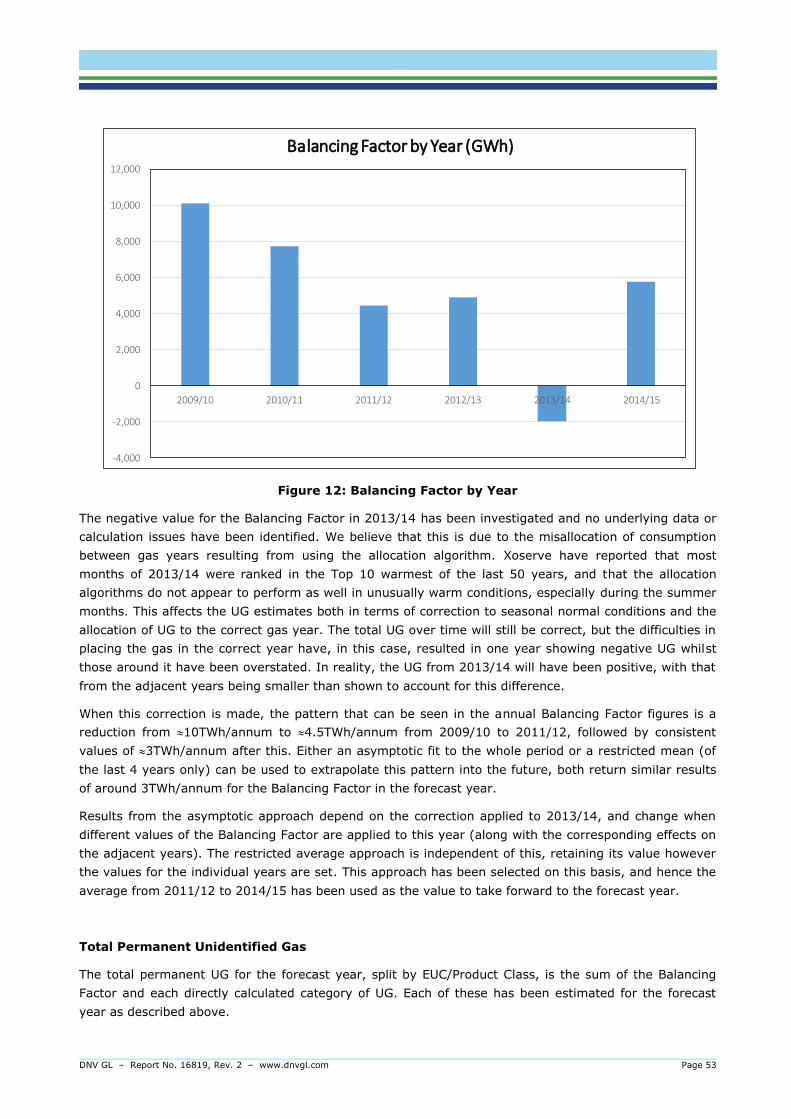
DNV GL – Report No. 16819, Rev. 2 – www.dnvgl.com Page 53
Figure 12: Balancing Factor by Year
The negative value for the Balancing Factor in 2013/14 has been investigated and no underlying data or
calculation issues have been identified. We believe that this is due to the misallocation of consumption
between gas years resulting from using the allocation algorithm. Xoserve have reported that most
months of 2013/14 were ranked in the Top 10 warmest of the last 50 years, and that the allocation
algorithms do not appear to perform as well in unusually warm conditions, especially during the summer
months. This affects the UG estimates both in terms of correction to seasonal normal conditions and the
allocation of UG to the correct gas year. The total UG over time will still be correct, but the difficulties in
placing the gas in the correct year have, in this case, resulted in one year showing negative UG whilst
those around it have been overstated. In reality, the UG from 2013/14 will have been positive, with that
from the adjacent years being smaller than shown to account for this difference.
When this correction is made, the pattern that can be seen in the annual Balancing Factor figures is a
reduction from 10TWh/annum to 4.5TWh/annum from 2009/10 to 2011/12, followed by consistent
values of 3TWh/annum after this. Either an asymptotic fit to the whole period or a restricted mean (of
the last 4 years only) can be used to extrapolate this pattern into the future, both return similar results
of around 3TWh/annum for the Balancing Factor in the forecast year.
Results from the asymptotic approach depend on the correction applied to 2013/14, and change when
different values of the Balancing Factor are applied to this year (along with the corresponding effects on
the adjacent years). The restricted average approach is independent of this, retaining its value however
the values for the individual years are set. This approach has been selected on this basis, and hence the
average from 2011/12 to 2014/15 has been used as the value to take forward to the forecast year.
Total Permanent Unidentified Gas
The total permanent UG for the forecast year, split by EUC/Product Class, is the sum of the Balancing
Factor and each directly calculated category of UG. Each of these has been estimated for the forecast
year as described above.
-4,000
-2,000
0
2,000
4,000
6,000
8,000
10,000
12,000
2009/10 2010/11 2011/12 2012/13 2013/14 2014/15
Balancing Factor by Year (GWh)

DNV GL – Report No. 16819, Rev. 2 – www.dnvgl.com Page 54
6.10 UG Factor Calculation
The final step in the calculation process is the production of the UG factors. These are a fundamental link
between the population of the EUC/Product Class combination and the UG from it.
They are therefore calculated using the detailed estimates of the value of UG (for the year in which the
factors will be in force) described in Section 6.9 above. Once the UG for each EUC/Product combination
for the forecast year has been estimated, this is converted into a factor by dividing it by the aggregate
AQ for that EUC/Product (i.e. the best estimate of the AQ for that EUC/Product combination for the
forecast year). This AQ data has been supplied to the AUGE by Xoserve. Therefore, each factor is
calculated as follows:
UG FactorPRODUCT,EUC = UG (GWh)PRODUCT,EUC / Aggregate AQ (TWh)PRODUCT,EUC
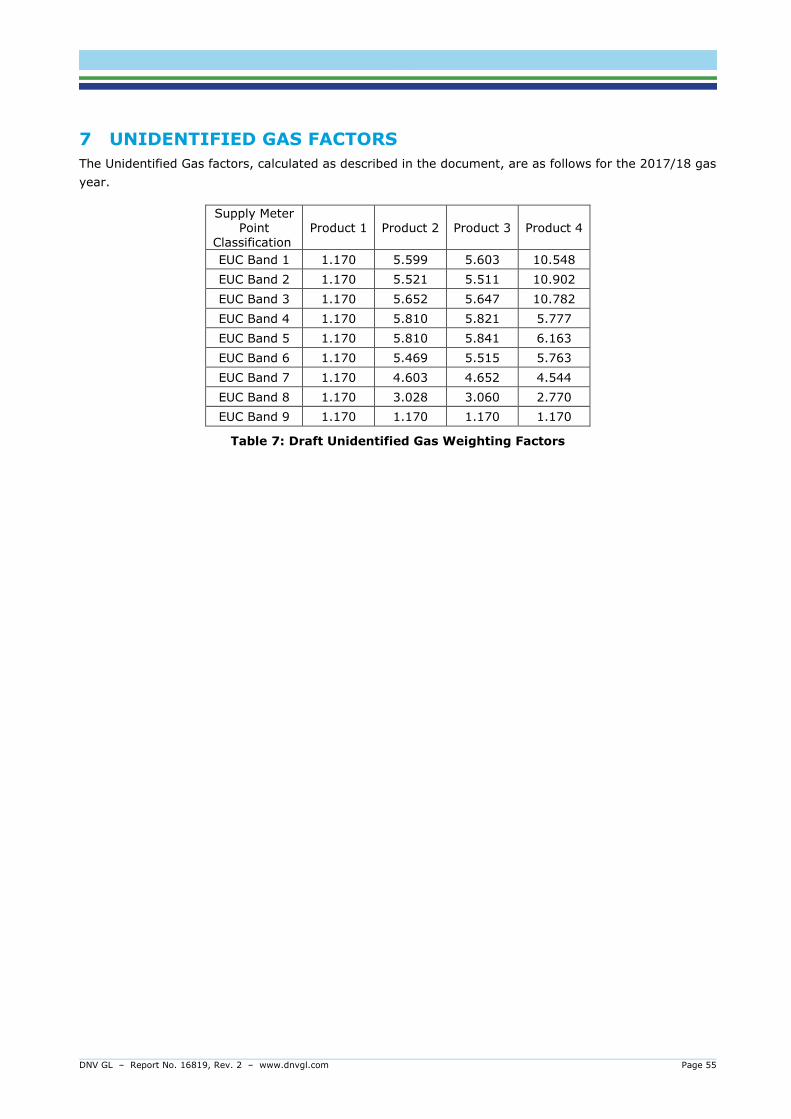
DNV GL – Report No. 16819, Rev. 2 – www.dnvgl.com Page 55
7 UNIDENTIFIED GAS FACTORS
The Unidentified Gas factors, calculated as described in the document, are as follows for the 2017/18 gas
year.
Supply Meter Point
Classification Product 1 Product 2 Product 3 Product 4
EUC Band 1 1.170 5.599 5.603 10.548
EUC Band 2 1.170 5.521 5.511 10.902
EUC Band 3 1.170 5.652 5.647 10.782
EUC Band 4 1.170 5.810 5.821 5.777
EUC Band 5 1.170 5.810 5.841 6.163
EUC Band 6 1.170 5.469 5.515 5.763
EUC Band 7 1.170 4.603 4.652 4.544
EUC Band 8 1.170 3.028 3.060 2.770
EUC Band 9 1.170 1.170 1.170 1.170
Table 7: Draft Unidentified Gas Weighting Factors
DNV GL – Report No. 16819, Rev. 2 – www.dnvgl.com Page 56
8 CONSULTATION QUESTIONS AND ANSWERS
This section captures a history of the questions raised by industry bodies during consultation periods and
the AUG Expert’s responses. These currently relate to the first draft of the 2017/18 AUG Statement only,
but this scope will expand as further consultation periods take place. The questions have been assessed
against the AUGE Guidelines Error! Reference source not found. and responses provided as
appropriate. All questions and answers have also been published on the Joint Office website.
Due to the in-depth nature of the questions raised and the detailed responses required, it is not
appropriate to publish full transcripts in this document. Instead, this section contains a summary of the
organisations that provided questions. The questions themselves and their associated responses can be
found in the following external documents:
“AUGS 2017-18 BG Response - DNVGL Comments” [20]
“AUGS 2017-18 ICoSS Response - DNVGL Comments” [21]
“AUGS 2017-18 E.ON Response - DNVGL Comments” [22]
Note that all responses contained in these documents relate to the UG calculations at the time they were
written, rather than reflecting the process as it currently stands. Therefore, wherever information differs
between the responses and the latest AUGS, this is because the UG analysis has evolved and information
in the response documents has been superseded. The information supplied in the latest version of the
AUGS is always the most up-to-date.
Organisation Name Date of Communication
British Gas 15/03/2017
ICoSS 15/03/2017
E.ON 15/03/2017
Table 8: Responses to the First Draft of the 2017/18 AUG Statement
9 CONTACT DETAILS
Questions can be raised with the AUGE at [email protected]
DNV GL – Report No. 16819, Rev. 2 – www.dnvgl.com Page 57
10 REFERENCES
[1] Framework for the Appointment of an Allocation of Unidentified Gas Expert V6.5, 21st January
2016
[2] Uniform Network Code – Transportation Principal Document Version 4.90, 01 October 2016
[3] Mod 0432: Project Nexus – Gas Demand Estimation, Allocation, Settlement and Reconciliation
reform, 17 January 2014
[4] Mod 0473/0473A: Project Nexus – Allocation of Unidentified Gas, 20 November 2014
[5] Standard Conditions of Gas Supply Licence (Gas Act 1986)
[6] CMA Energy market investigation, Final report, 24 June 2016
[7] Mod 0424: Re-establishment of Supply Meter Points – prospective measures to address
Shipperless sites, 20 December 2012
[8] Mod 0425V: Re-establishment of Supply Meter Points – Shipperless sites, 7 January 2014
[9]
Mod 0410/0410A: Responsibility for gas off-taken at Unregistered Sites following New Network
Connections, 12 July 2013
[10] 2011 Allocation of Unidentified Gas Statement for 2012/13
[11] Mod 0594R: Meter Reading Submission for Advanced & Smart Metering, 15 September 2016
[12] Mod 0572: Amendment to the definition of AUG Year within UNC TPD Section E
[13] iGT 053: Introduction of annual updates to the AQ values within the CSEP NExA table, 1
October 2014
[14] Mod 0398: Limitation on Retrospective Invoicing and Invoice Correction (3 to 4 year solution),
1 April 2014
[15] Project Nexus Workgroup Volumetric Assumptions, Xoserve presentation, 24 July 2015
[16] Energy UK Gas Retail Group Study into the effect of shrinkage on domestic customers, October
2015
[17] Department for Business, Energy & Industrial Strategy: Smart Meters Quarterly Report to end
September 2016, 22 December 2016
[18] Department for Business, Energy & Industrial Strategy: Smart Meter Roll-Out Cost-Benefit
Analysis, August 2016
[19] LDZ Shrinkage Quantity Proposals, 2009/10 to 2017/18,
http://www.gasgovernance.co.uk/Shrinkage/Shrinkage-Quantity-Proposals
[20] AUGS 2017-18 BG Response - DNVGL Comments, April 2017
[21] AUGS 2017-18 ICoSS Response - DNVGL Comments, April 2017
[22] AUGS 2017-18 E.ON Response - DNVGL Comments, April 2017
DNV GL – Report No. 16819, Rev. 2 – www.dnvgl.com Page 58
GLOSSARY
AGI Above Ground Installation
ALP Annual Load Profile (deeming algorithm parameter)
AMR Automated Meter Reading
AQ Annual Quantity. An estimate of annual consumption under seasonal normal
conditions
AUG Allocation of Unidentified Gas
AUGE Allocation of Unidentified Gas Expert
AUGS Allocation of Unidentified Gas Statement
Balancing Factor An aggregate of the combined Unidentified Gas of various items calculated by
subtraction. This includes theft, errors in the shrinkage estimate, open bypass
valves, meters “Passing Unregistered Gas”, unknown sites, and additional
common cause variation.
CMA Competition & Markets Authority
Consumption Method Unidentified Gas methodology using meter reads and metered volumes
CSEP Connected System Exit Point
CV Calorific Value
CWAALP Cumulative Weather Adjusted Annual Load Profile
CWV Composite Weather Variable
DAF Daily Adjustment Factor (deeming algorithm parameter)
DM Daily Metered
DME Daily Metered Elective. A site below the DM mandatory threshold of 58,600,000
kWh which the shipper has elected to be DM. The meter read equipment is
provided by the shipper.
DMM Daily Metered Mandatory. A site with an AQ above the DM mandatory threshold
of 58,600,000 kWh.
DMV Daily Metered Voluntary. A site below the DM mandatory threshold of
58,600,000 kWh which is voluntarily DM. The meter read equipment is provided
by the transporter.
ECV Emergency Control Valve
EUC End User Category
EWCF Estimated Weather Correction Factor (deeming algorithm output - alternative to
WCF based on CWV rather than demand)
Found Meter A meter being supplied by a Shipper but for which Xoserve have no record
GFD Gas Flow Day
DNV GL – Report No. 16819, Rev. 2 – www.dnvgl.com Page 59
GSR Gas Safety Regulations
IGT Independent Gas Transporter
Isolated Meter A meter that has been disabled (through capping or clamping) and hence is no
longer capable of flowing gas, and this information has been conveyed to
Xoserve and recorded on their system.
LDZ Local Distribution Zone
LSP Larger Supply Point
MAM Meter Asset Manager
Model Error The statistical error associated with any modelling or estimation process. It an
inherent part of any statistical model and does not imply that the model itself is
inadequate or incorrect.
MPRN Meter Point Reference Number
NDM Non-Daily Metered
ODR OFGEM Data Request
OUG Own Use Gas
PSND Pseudo Seasonal Normal Demand, calculated using AQ values rather than being
based on historic metered demands
PTS Passed To Shipper
RbD Reconciliation by Difference
RPD Meter Rotary Positive Displacement meter
SAP System Average Price
SF Scaling Factor (deeming algorithm output)
SNCWV Seasonal Normal Composite Weather Variable
SND Seasonal Normal Demand
SPC Supply Point Component
SSP Smaller Supply Point
SSrP Shipper Specific rePort
TPD Transportation Principal Document (of UNC)
UIP Utility Infrastructure Provider
UNC Uniform Network Code
UG Unidentified Gas
UIG UNC definition of total Unidentified Gas calculated on a daily basis as part of the
settlement process
WAALP Weather Adjusted Annual Load Profile

DNV GL – Report No. 16819, Rev. 2 – www.dnvgl.com Page 60
WCF Weather Correction Factor (deeming algorithm output)
WSENS Weather Sensitivity (deeming algorithm parameter used in EWCF definition,
reflecting the sensitivity of an EUC to difference in CWV from seasonal normal)

DNV GL – Report No. 16819, Rev. 2 – www.dnvgl.com A-1
APPENDIX A
Data
This appendix describes the raw data provided by Xoserve for the consumption method.
ALLOCATIONS
This data contains all allocations including CSEPs from 01/10/2008 onwards.
Name Description
GAS_DAY Date - Gas day for which allocation applies
LDZ Char[2] - LDZ identifier e.g. EA
EUC Char[11] - Full EUC Code e.g. WM:E0708W02
ALLOCATED_ENERGY Number - Final allocated energy value (kWh). Includes CSEPs
ANNUAL_QUANTITY
This data includes all meter points active at any point from 01/10/2008 onwards, not just those currently
live. It includes all within gas year updates, appeals etc.
Name Description
MPR_ID Number – Unique dummy ID for meter point which is used
consistently throughout the data
AQ_EFFECTIVE_DATE Date - Date on which AQ becomes effective
EUC Char[11] - Full EUC Code e.g. WM:E0708W02
AQ Number - Annual Quantity to apply from effective date (kWh)
SITE_TYPE_FLAG Char[1] - Indicator ="N" for NDM meter point, "D" for DM meter
point or "U" for Unique site
CSEPS
This data contains information for gas year 2008 onwards.
Name Description
GAS_YEAR Date - Gas year for which CSEP AQ/Numbers apply
EUC* Char[11] - Full EUC Code e.g. WM:E0708W02
TOTAL_AQ Number - Aggregate CSEP AQ at start of gas year
COUNT_OF_SUPPLY_POINTS Number - Count of supply points at start of gas year
* Note that the EUC classification for CSEPs is based on a nominal maximum AQ
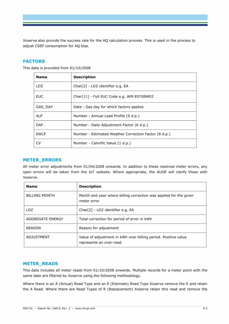
DNV GL – Report No. 16819, Rev. 2 – www.dnvgl.com A-2
Xoserve also provide the success rate for the AQ calculation process. This is used in the process to
adjust CSEP consumption for AQ bias.
FACTORS
This data is provided from 01/10/2008
Name Description
LDZ Char[2] - LDZ identifier e.g. EA
EUC Char[11] - Full EUC Code e.g. WM:E0708W02
GAS_DAY Date - Gas day for which factors applies
ALP Number - Annual Load Profile (6 d.p.)
DAF Number - Daily Adjustment Factor (6 d.p.)
EWCF Number - Estimated Weather Correction Factor (8 d.p.)
CV Number - Calorific Value (1 d.p.)
METER_ERRORS
All meter error adjustments from 01/04/2008 onwards. In addition to these resolved meter errors, any
open errors will be taken from the JoT website. Where appropriate, the AUGE will clarify these with
Xoserve.
METER_READS
This data includes all meter reads from 01/10/2008 onwards. Multiple records for a meter point with the
same date are filtered by Xoserve using the following methodology.
Where there is an A (Actual) Read Type and an E (Estimate) Read Type Xoserve remove the E and retain
the A Read. Where there are Read Types of R (Replacement) Xoserve retain this read and remove the
Name Description
BILLING MONTH Month and year where billing correction was applied for the given
meter error
LDZ Char[2] - LDZ identifier e.g. EA
AGGREGATE ENERGY Total correction for period of error in kWh
REASON Reason for adjustment
ADJUSTMENT Value of adjustment in kWh over billing period. Positive value
represents an over-read
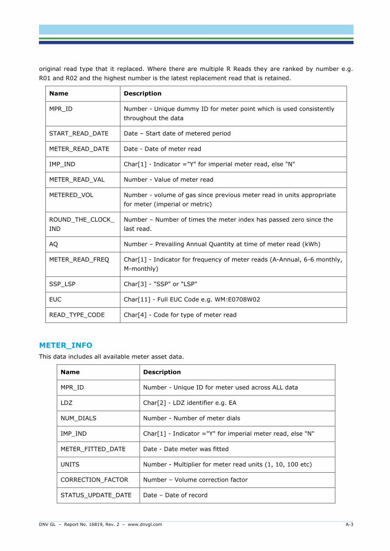
DNV GL – Report No. 16819, Rev. 2 – www.dnvgl.com A-3
original read type that it replaced. Where there are multiple R Reads they are ranked by number e.g.
R01 and R02 and the highest number is the latest replacement read that is retained.
METER_INFO
This data includes all available meter asset data.
Name Description
MPR_ID Number - Unique ID for meter used across ALL data
LDZ Char[2] - LDZ identifier e.g. EA
NUM_DIALS Number - Number of meter dials
IMP_IND Char[1] - Indicator ="Y" for imperial meter read, else "N"
METER_FITTED_DATE Date - Date meter was fitted
UNITS Number - Multiplier for meter read units (1, 10, 100 etc)
CORRECTION_FACTOR Number – Volume correction factor
STATUS_UPDATE_DATE Date – Date of record
Name Description
MPR_ID Number - Unique dummy ID for meter point which is used consistently
throughout the data
START_READ_DATE Date – Start date of metered period
METER_READ_DATE Date - Date of meter read
IMP_IND Char[1] - Indicator ="Y" for imperial meter read, else "N"
METER_READ_VAL Number - Value of meter read
METERED_VOL Number - volume of gas since previous meter read in units appropriate
for meter (imperial or metric)
ROUND_THE_CLOCK_
IND
Number – Number of times the meter index has passed zero since the
last read.
AQ Number – Prevailing Annual Quantity at time of meter read (kWh)
METER_READ_FREQ Char[1] - Indicator for frequency of meter reads (A-Annual, 6-6 monthly,
M-monthly)
SSP_LSP Char[3] - "SSP" or "LSP"
EUC Char[11] - Full EUC Code e.g. WM:E0708W02
READ_TYPE_CODE Char[4] - Code for type of meter read
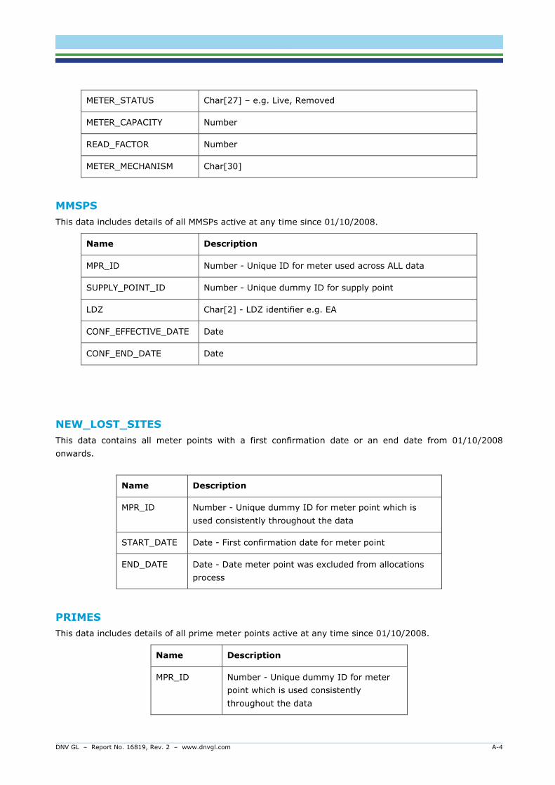
DNV GL – Report No. 16819, Rev. 2 – www.dnvgl.com A-4
METER_STATUS Char[27] – e.g. Live, Removed
METER_CAPACITY Number
READ_FACTOR Number
METER_MECHANISM Char[30]
MMSPS
This data includes details of all MMSPs active at any time since 01/10/2008.
Name Description
MPR_ID Number - Unique ID for meter used across ALL data
SUPPLY_POINT_ID Number - Unique dummy ID for supply point
LDZ Char[2] - LDZ identifier e.g. EA
CONF_EFFECTIVE_DATE Date
CONF_END_DATE Date
NEW_LOST_SITES
This data contains all meter points with a first confirmation date or an end date from 01/10/2008
onwards.
Name Description
MPR_ID Number - Unique dummy ID for meter point which is
used consistently throughout the data
START_DATE Date - First confirmation date for meter point
END_DATE Date - Date meter point was excluded from allocations
process
PRIMES
This data includes details of all prime meter points active at any time since 01/10/2008.
Name Description
MPR_ID Number - Unique dummy ID for meter
point which is used consistently
throughout the data
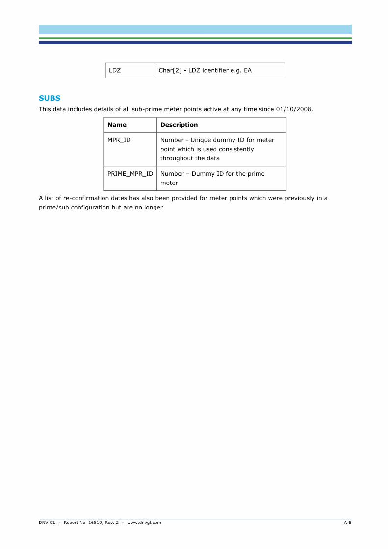
DNV GL – Report No. 16819, Rev. 2 – www.dnvgl.com A-5
LDZ Char[2] - LDZ identifier e.g. EA
SUBS
This data includes details of all sub-prime meter points active at any time since 01/10/2008.
Name Description
MPR_ID Number - Unique dummy ID for meter
point which is used consistently
throughout the data
PRIME_MPR_ID Number – Dummy ID for the prime
meter
A list of re-confirmation dates has also been provided for meter points which were previously in a
prime/sub configuration but are no longer.


About DNV GL Driven by our purpose of safeguarding life, property and the environment, DNV GL enables organizations to advance the safety and sustainability of their business. We provide classification and technical assurance along with software and independent expert advisory services to the maritime, oil & gas and energy industries. We also provide certification services to customers across a wide range of industries. Operating in more than 100 countries, our professionals are dedicated to helping our customers make
the world safer, smarter and greener.