alternative optimized monetary policy rules in multi ...alternative optimized monetary policy rules...
TRANSCRIPT

Working Paper/Document de travail 2010-9
Alternative Optimized Monetary Policy Rules in Multi-Sector Small Open Economies: The Role of Real Rigidities
by Carlos de Resende, Ali Dib, and Maral Kichian

2
Bank of Canada Working Paper 2010-9
March 2010
Alternative Optimized Monetary Policy Rules in Multi-Sector Small Open
Economies: The Role of Real Rigidities
by
Carlos de Resende,1 Ali Dib,1 and Maral Kichian2
1International Economic Analysis Department Bank of Canada
Ottawa, Ontario, Canada K1A 0G9 [email protected]
2Canadian Economic Analysis Department Bank of Canada
Ottawa, Ontario, Canada K1A 0G9 [email protected]
Bank of Canada working papers are theoretical or empirical works-in-progress on subjects in economics and finance. The views expressed in this paper are those of the authors.
No responsibility for them should be attributed to the Bank of Canada.
ISSN 1701-9397 © 2010 Bank of Canada
ii
Acknowledgements
We would like to thank Kosuke Aoki, Mick Devereaux, Jean-Marie Dufour, Luca Guerrieri, Hashmat Khan, Sharon Kozicki, Jocelyn Jacob, Robert Lafrance, James Rossiter, Malik Shukayev, Gregor Smith, Alexander Ueberfeldt, as well as seminar participants at the Bank of Canada, the Central Bank of Brazil, the 2008 SOEGW conference, the 2009 meeting of the Canadian Economic Association, the 2009 meeting of the Society for Computational Economics, and the 2009 Central Bank Macroeconomic Modeling.

iii
Abstract
Inflation-targeting central banks around the world often state their inflation objectives with regard to the consumer price index (CPI). Yet the literature on optimal monetary policy based on models with nominal rigidities and more than one sector suggests that CPI inflation is not always the best choice from a social welfare perspective. We revisit this issue in the context of an estimated multi-sector New-Keynesian small open economy model where sectors are heterogeneous along multiple dimensions. With key parameters of the model estimated using data from an inflation targeting economy, namely Canada, we particularly focus on (i) the role of sector-specific real rigidities, specially in the form of factor mobility costs, and (ii) welfare implications of targeting alternative price indices. Our estimations reveal considerable heterogeneity across sectors, and in several dimensions. Moreover, in contrast to existing studies, our welfare analysis comparing simple optimized policy rules based on alternative sectoral inflation rates provides support for CPI-based targeting policies by central banks. Capital mobility costs matter importantly in this regard.
JEL classification: E4, E52, F3, F4 Bank classification: Inflation: costs and benefits; Inflation and prices; Inflation targets; Monetary policy framework; Monetary policy implementation
Résumé
Les banques centrales de par le monde qui poursuivent des cibles d’inflation fixent fréquemment leurs objectifs par référence à l’indice des prix à la consommation (IPC). Or, selon la littérature qui fait appel, pour l’analyse de la politique monétaire optimale, à des modèles multisectoriels englobant des rigidités nominales, l’IPC ne serait pas toujours le meilleur étalon sous l’aspect du bien-être social. Les auteurs examinent de nouveau la question en se servant d’un modèle de type nouveau keynésien représentant une petite économie ouverte composée de plusieurs secteurs hétérogènes à différents égards. Ils estiment les principaux paramètres du modèle au moyen de données tirées d’une économie à régime de cibles d’inflation, en l’occurrence le Canada. Ils étudient notamment le rôle des rigidités réelles sectorielles, tout particulièrement sous forme de coûts de mobilité des facteurs, et les conséquences pour le bien-être du choix d’indices de prix autres que l’IPC. Leurs estimations révèlent une hétérogénéité intersectorielle appréciable, et ce, à plusieurs titres. Qui plus est, leur analyse du bien-être, fondée sur une comparaison de règles de politique monétaire simples et optimales sur la base de différents taux d’inflation sectoriels, accrédite les politiques de ciblage de l’inflation d’après l’IPC pratiquées par les banques centrales, à l’opposé des études antérieures. Les coûts de mobilité du capital sont déterminants à ce chapitre.
Classification JEL : E4, E52, F3, F4 Classification de la Banque : Inflation : coûts et avantages; Inflation et prix; Cibles en matière d’inflation; Cadre de la politique monétaire; Mise en œuvre de la politique monétaire

1 Introduction
The nineties witnessed a substantial increase in the number of countries adopting inflation-targeting
as their main monetary policy framework. These countries with explicitly-announced inflation
targets often stated those objectives based on the consumer price index (CPI).1 Yet, the literature
on optimal monetary policy based on dynamic models with multiple sources of nominal rigidities
(Erceg et al. 2000, Mankiw and Reis 2002; Woodford 2003; Benigno 2004; Huang and Liu 2005)
suggests that the CPI inflation is not always the best choice from a social welfare perspective. This
is the case because, unlike models with a single source of nominal rigidity (Aoki 2001), multi-sector
models with sectoral heterogeneity in price and/or wage rigidities display a trade-off between the
stabilization of deviations of output from its steady-state value (hereafter refered to as the output
gap) and multiple sectoral relative prices, which are not allocative-neutral. This trade-off implies
that stabilization of CPI inflation does not necessarily mean stabilization of the output gap.
In this paper, we revisit the choice of CPI inflation as an optimal guide to monetary policy
in the context of an estimated multi-sector New-Keynesian small open economy model with four
sectors (manufacturing, non-tradable, commodity, and imported goods) that are heterogeneous with
respect to: (i) the degree of price and wage nominal rigidity, (ii) labour inputs, (ii) the adjustment
cost of capital, and (iv) the stochastic process underlying the technology shocks. In particular,
we use the welfare implications of the model to quantitatively assess the relative merits of simple,
implementable policy reaction functions that include targeting the inflation rate of an aggregate
price index (e.g., CPI) versus a sectoral price index (e.g., tradables, nontradables, imports).
Our contribution to the debate regarding which price is the most desirable to target is two-
fold. First, in contrast with the existing literature which focuses on nominal rigidities, we highlight
the role of real rigidities in the form of factor mobility costs. As sectors differ with respect to
their degree of nominal rigidities and the economy is hit by sector-specific shocks, monetary policy
will have asymmetric effects in different sectors, with potential allocative implications. To the
extent that sectoral (re)allocation of resources becomes costly due to the introduction of imperfect
labour mobility and sector-specific capital, we are able to explore another source of welfare loss
in the economy, which will add to the losses induced by nominal rigidities and by monopolistic
competition (i. e., price dispersion and suboptimal output) extensively discussed in the literature.
Second, the existing literature (see, for example, Beningo 2004) emphasizes that the optimal
price index to target will depend on the interplay between the shares of the different sectors in the
economy and the differences in the sectoral degrees of nominal rigidities. Our conjecture is that
the extent of sector-specific capital adjustment costs should also matter in this regard. How much
it matters is a quantitative question and, for this reason, it becomes important to use parameter
1These include, for example, Canada, New Zealand, United Kingdom, Finland, Sweden, Spain, France, Germany,
and Switzerland; a few of these targeting CPI without the effects of indirect taxes and mortgage interest payments.
1
values that reflect the reality of a well-established inflation-targeting economy in order to study
the welfare implications of targeting alternative price indices within policy reaction functions. We
follow the numerical approach used in Kollmann (2002), Ambler et al. (2004), Bergin et al. (2007),
and Schmitt-Grohe and Uribe (2007) to calculate optimized policy functions in which the monetary
authority optimally chooses the Taylor rule coefficients to stabilize inflation and output.2 In this
paper, we focus on the case of Canada to estimate our key parameters.3
Furthermore, although the main motivation for including real rigidities into the factor structure
is the need to capture some arguably realistic assumptions regarding the limited transferability of
labour skills and capital across sectors, Christiano, Eichenbaum, and Evans (2005) and Eichenbaum
and Fisher (2007) suggest a further reason for using imperfectly-mobile capital with capital adjust-
ment costs in estimated medium-scale dynamic stochastic general equilibrium models. They argue
that these features help generate average frequencies of price adjustments that are much more in
line with values obtained from micro-based studies.
Since we use Canada as our benckmark inflation-targeting economy, a number of additional
features have been introduced in the model to better replicate important aspects of the Canadian
economy. For instance, we consider a monopolistically competitive importing sector that distributes
differentiated goods imported from Canada’s main trading partner − the United States − and therest of the world. This distinction among trade partners is important because of the pre-eminent
role played by the Canada-U.S. bilateral exchange rate in the dynamics of the various components
of Canadian inflation. In addition, as the price in the importing sector (expressed in domestic
currency) also displays stickiness, our set-up takes into account the evidence of incomplete exchange
rate pass-through in Canada (see, for example, Gagnon and Ihrig 2004).
In the same spirit, we introduce a commodity sector that uses labour, capital, and natural
resource endowment (“land”). As Canada is a net exporter of this type of good, commodity prices
exogenously determined in the world economy have important effects on the real exchange rate
and, thus, on inflation. Because commodity goods are used as inputs in the production of other
sectors, they contribute to the (incomplete) pass-through of shocks to commodity prices into the
Canadian economy.4
We also consider aspects related to the current globalized world economy that are likely to affect
our small open economy directly. Thus, while we do not explain globalization itself, we account for
2As pointed out by De Paoli (2009), such a numerical approach is useful to evaluate optimal policy in complex and
fairly realistic open economy settings. An alternative would have been to examine the role of real rigidities within a
simpler framework and considering an analytical representation of the monetary authorithy’s problem as in Benigno
(2004).3While our model is calibrated and estimated using Canadian data, its structure and the results would equally
apply to other commodity-exporting small open economies such as Australia, New Zealand, and Norway.4See Dib (2008) for the importance of having such a commodities sector in a small open-economy model for
Canada. See also Bouakez, Cardia, and Ruge-Murcia (2009) who use input-output tables to describe in even finer
detail the various levels of production.
2

the possibility that relatively-persistent shocks from foreign sources can directly and markedly alter
the import and tradable sectors of our economy. Examples of such shocks can be, for instance, the
removal or addition of trade quotas and tariffs, changes in home bias and tastes, improvements in
the quality of imported goods, and declines in import costs due to increased internationalization
and the opening-up of new markets, that can potentially alter trade flows importantly.
We estimate key structural parameters of the model using Bayesian methods as in Smets and
Wouters (2003, 2007). We focus on parameters with a sector-specific dimension, such as Calvo-
price and -wage rigidities, capital adjustment costs, and the stochastic processes for exogenous
technology shocks, as well as the processes for the shocks to foreign variables. Our estimations find
support for significant heterogeneity across sectors and along many dimensions. In particular, the
sector that produces nontradable goods stands out as the one with the most rigid prices and wages,
with the most costly stock of capital to adjust, and with the most persistent and volatile technology
shock. As that sector’s production is also the one with the highest share in the Canadian economy,
its underlying characteristics turn out to be very important for our results.
Using the estimated parameters, we next solve the model’s equilibrium conditions to a second-
order approximation around the deterministic steady-state and compare the welfare implications
of five alternative monetary policy rules. We focus on policy reaction functions with a “smoothing
term,” whereby the central bank changes the nominal interest rate in reaction to last period’s
interest rate, current inflation and the output gap. The alternative options differ with respect to
the price index or inflation rate targeted by the monetary authority.5 Ortega and Rebei (2006),
using a similar approach in a two-sector model without sector-specific capital adjustment costs find
that the best option is to target the inflation rate of nontradables, which they also identify as the
sector with the stickiest prices. In contrast, our main finding is that the highest welfare level is
achieved by targeting CPI inflation rather than any of the inflation rates of the remaining sectors,
thus confirming the soundness of CPI-based targeting policy by the Bank of Canada. The ranking
of policies is maintained when price-level targeting is considered. Interestingly, when we shut down
the capital adjustment costs, targeting the inflation rate of the nontradable sector becomes the best
option, which highlights the importance of real rigidities in this regard.
The paper is organized as follows. Section 2 presents the main features of the model. Section 3
describes the data, the calibration of selected parameters, as well as the estimation results. Section
4 reports and discusses the simulation results of the model. Section 5 offers some conclusions.
5 In all our welfare calculations policy reaction functions include deviations of inflation (price index) from its
steady-state value which is calibrated to reflect the target level of inflation (price index).
3

2 The Model
We consider a variant of the small open economy model proposed by Dib (2008) for Canada, which
builds upon earlier work by Mendoza (1991), Erceg, Henderson and Levin (2000), and Kollmann
(2001).6 The economy consists of households, a government, a monetary authority (or central bank),
and a multi-tiered production sector. The latter is structured as follows: a domestic commodity
sector exports some of its production and supplies the rest domestically to the manufacturing
and the non-tradables sectors of the economy. The manufacturing sector produces goods that are
exported or used domestically, and the non-tradables sector produces goods that are destined only
for the local market. Foreign goods are imported from different external sources and combined with
manufactured goods to yield an aggregate tradable good. The final stage of the production process
consists in aggregating tradable and non-tradable goods in order to produce final consumption
goods.7
Households set monopolistically competitive wages. Monopolistic competition is also assumed in
all the intermediate stages of production, while perfect competition is considered in the commodities
and final goods’ markets. In addition, various nominal rigidities are allowed in the economy. Wages,
as well as domestic, imported, intermediate, and final goods’ prices are considered to be sticky à la
Calvo-Yun.
2.1 Households
Households in the economy are represented by a continuum indexed by ∈ [0 1]. Each household has preferences defined over consumption, , and labour hours, , described by:
0
∞X=0
()
where 0 denotes the mathematical expectations operator conditional on information available at
period 0, is the subjective discount factor, and (·) is a utility function that is strictly concave,strictly increasing in , and strictly decreasing in .
The instantaneous utility function is given by
(·) = 1−
1− −
1+
1 + (1)
with =
∙
1+
+1+
+1+
¸ 1+
, where , , and , represent hours worked
by the household in manufacturing, non-tradable, and commodity sectors, which are indexed
by , and , respectively. In addition, is the inverse of the elasticity of intertemporal
6A related paper that estimates a DSGE model using Canadian data is Justiniano and Preston (2009).7Bouakez, Cardia, and Ruge-Murcia (2009) show that estimated models using a more detailed production structure
can better approximate sectoral nominal rigidities.
4
substitution of consumption, denotes the labour elasticity of substitution across sectors, and is
the inverse of the Frisch wage elasticity of labour supply. All three parameters are assumed to be
strictly positive. Note that, except in the limit case where →∞, the household ’s labour supply,, is different from
P= , which implies that households do not perfectly substitute
their hours worked in the different sectors.
Household is a monopolistic supplier of differentiated labour services, selling these to a rep-
resentative competitive firm (a union) that transforms these into aggregate labour inputs for each
sector (=) according to the technology:
=
µZ 1
0
−1
¶ −1
= (2)
In the above, , , and denote aggregate labour supplied to manufacturing, non-
tradable, and commodity sectors, respectively, and the elasticity of substitution among the types of
labour is given by 1. From the labour union’s optimization problem, labour demand in sector
is described by the equation
=
µ
¶− (3)
with as the nominal wage of household when working for sector . The nominal wage index
in sector , , is thus given by:
=
µZ 1
0
()1−
¶ 11−
(4)
Households can buy or sell bonds denominated in foreign currency in incomplete international
financial markets. We assume that all international bonds are denominated in U.S. dollars (USD)
and denote as the nominal exchange rate between Canadian dollars (CAD) and USD. Household
enters period with units of capital in the sector , −1 units of domestic treasury bonds,
and ∗−1 units of foreign bonds denominated in USD, where
is the U.S. price level and ∗
is the (real) foreign debt of the economy. During period the household supplies labour and capital
to firms in all production sectors, receives total factor paymentP
=( +),
where is the nominal rental rate of capital in the sector , and receives factor payment of
natural resources, , where is the nominal price of the natural resource input, , and
is the share of the household in natural resource payments.8 Furthermore, household pays
a lump-sum tax Υ to the government and receives dividend payments from intermediate goods
producing firms, . The household uses some of its funds to purchase the final good at the
nominal price , which it then divides between consumption and investment in each production
sector.
8Note that, 10 = 1.
5
Accordingly, the budget constraint of household is given by:
( + ) +
+
∗
∗
≤X
=
¡
+
¢+−1 +
−1∗−1 + + −Υ (5)
where = ++ is total investment in the manufacturing, non-tradable, and commodity
sectors, respectively; and = + + is the total profit from the manufacturing,
non-tradable and import sectors.
The foreign bond return rate, ∗ , depends on the foreign interest rate ∗ and a country-
specific risk premium . The foreign interest rate evolves exogenously according to the following
AR(1) process:
log(∗ ) = (1− ∗) log(∗) + ∗ log(
∗−1) + ∗ (6)
where ∗ 1 is the steady-state value of ∗ , ∗ ∈ (−1 1) is an autoregressive coefficient, and∗ is uncorrelated and normally distributed innovation with zero mean and standard deviations
∗ .
The country-specific risk premium is increasing in the foreign-debt-to-GDP ratio. It is given by
= exp
µ−κ
∗
¶ (7)
where κ 0 is a parameter that determines the ratio of foreign debt to GDP, and is total real
GDP. The introduction of this risk premium ensures that the model has a unique steady state. It
is assumed that the U.S. inflation rate, ∗ =
−1, evolves according to:
log(∗ ) = (1− ∗) log(∗) + ∗ log(
∗−1) + ∗ (8)
where ∗ 1 is the steady-state value of ∗ , ∗ ∈ (−1 1) is an autoregressive coefficient, and ∗is an uncorrelated and normally distributed innovation with zero mean and standard deviations
∗ .
The stock of capital in the sector evolves according to:
+1 = (1− ) + −Ψ(+1) (9)
where ∈ (0 1) is the capital depreciation rate common to all sectors andΨ(·) = 2
³+1
− 1´2
is sector ’s capital-adjustment cost function that satisfies Ψ(0) = 0, Ψ0(·) 0 and Ψ00(·) 0. Since
capital is sector-specific and costly to adjust, moving capital between two sectors requires adjust-
ment costs to be paid both in the sector that is investing and in the sector where the capital stock
is being reduced.
6

Household chooses +1 and ∗ to maximize its lifetime utility, subject to Eqs.
(5) and (9). The first-order conditions, expressed in real terms, are:
− = ; (10)
∙+1
µ+1 + 1− +
µ+2
+1
− 1¶+2
+1
−
2
µ+2
+1
− 1¶2!#
=
µ+1
− 1¶+ 1 =; (11)
=
∙+1
+1
¸; (12)
∗
=
∙+1
+1
∗+1
¸ (13)
in addition to the budget constraint, Eq. (5), to which the Lagrangian multiplier, , is associated;
= , = −1, and =
denote real capital return in the sector , the
domestic CPI inflation rate, and the bilateral CAD/USD real exchange rate, respectively. Equations
(12) and (13) together imply the uncovered interest rate parity (UIP) condition:
∗
=
+1
(14)
Furthermore, there are three first-order conditions for setting nominal wages in each sector ,f, when household is allowed to revise its nominal wages. As in Calvo (1983), this happens
with probability (1 − ) in the sector , at the beginning of each period . If household is not
allowed to change its nominal wage, it fully indexes its wage to the steady-state inflation rate, , as
in Yun (1996). Following Schmitt-Grohé and Uribe (2007), household sets his optimized nominal
wage in the sector , f, to maximize the flow of its expected utility, so that
max
0
" ∞X=0
()n (++) + +
f++
o#
subject to + =
µ
+
¶−+, where = . The first-order condition derived forf is
0
⎡⎣ ∞X=0
() +
Ãf
+
!−+
(+ −
− 1
f
+
)⎤⎦ = 0 (15)
where = −
is the marginal rate of substitution between consumption and labour type
. Dividing Eq. (15) by and rearranging yields:
e =
− 1
P∞=0()
++++
Q=1
−+
P∞=0()
+++
Q=1
(1−)−1+
(16)
7
where e = f and = are the household ’s real optimized wage and real wage
index in the sector , respectively.
The nominal wage index in the sector evolves over time according to the following recursive
equation:
()1− = (−1)1− + (1− )(
f)1− (17)
where f is the average wage of those workers who are allowed to revise their wage at period in
the sector . Dividing (17) by yields:
()1− =
µ−1
¶1−+ (1− )( e)
1− (18)
In a symmetric equilibrium, e = e and = for all . Therefore, we can rewrite
equation. (16) in a non-linear recursive form following Schmitt-Grohé and Uribe (2007):
e =
− 11
2; (19)
where
1 =
" ∞X=0
() +++
+
Y=1
−+
#;
= +
h(+1)
1+1
i; (20)
and
2 =
" ∞X=0
() ++
+
Y=1
(1−))−1+
#;
= +
h(+1)
−12+1i (21)
In addition, Eqs. (16) and (18) permit us to derive the standard New Keynesian Phillips curve,
= +1 +(1−)(1−)
[ − ], where
= −1 is wage inflation in the sector
and hats over the variables denote deviations from steady-state values.
2.2 Final good
To facilitate the exposition of the production structure, we start from the final stage of produc-
tion (explained in this section) and move through the intermediate phase to the initial stages of
production. Diagram 1 displays the production structure of the model.
At the last stage of production, a perfectly-competitive representative firm combines a com-
posite tradable good, , and non-tradable goods, , with corresponding prices and ,
respectively, using the following CES function to produce a homogeneous final good, :
=
∙(1− )
1
−1
+ 1
−1
¸ −1
(22)
8
where is the share of non-tradables in the final good and 0 is the elasticity of substitution
between non-tradable and tradable goods.
Taking the price of the final good, , as given, the final good producer chooses and
to maximize its profit. Formally:
max{}
− −
subject to (22). Profit maximization implies the following demand functions for the aggregate
tradable good and the non-tradable good:
= (1− )
µ
¶− and =
µ
¶− (23)
The zero-profit condition implies that the final-good price level, which we interpret as the
consumer-price index (CPI), is linked to tradable and non-tradable goods’ prices via the equation:
=h(1− )
1− +
1−
i1(1−) (24)
2.3 The non-tradable sector
Wholesale producers. The non-tradable good input used to produce in (22) is generated
by a competitive wholesale firm that aggregates differentiated goods produced by a continuum of
intermediate good producers which are indexed by ∈ [0 1]. The wholesale firm uses the following
CES technology:
=
µZ 1
0
()−1
¶ −1
(25)
where is the demand for intermediate input and 1 is the constant elasticity of substitution
between the differentiated goods. The maximization problem of the wholesaler is given by:
max{}
−Z 1
0
subject to (25). The solution to this problem implies a demand function and a corresponding price,
, of the differentiated good, given, respectively, by:
=
µ
¶− (26)
and
=
µZ 1
0
()1−
¶ 11−
(27)
9
Intermediate good producers. Each intermediate good firm in sector produces output,
, using capital, (=R 10), labour, (=
R 10), and a commodity input,
. The production function is represented by the following Cobb-Douglas technology:
≤ () ()
¡
¢ ∈ (0 1) (28)
where + + = 1; , , and are shares of capital, labour, and commodity inputs
in the production of non-tradable goods, respectively. is a technology shock specific to the
non-tradable sector. It is assumed that this shock evolves exogenously according to:
log() = (1− ) log() + log(−1) + (29)
where 0 is the steady-state value of , ∈ (−1 1) is an autoregressive coefficient, and is uncorrelated and normally distributed innovation with zero mean and standard deviations
.
As in the wage-setting decisions of households, Calvo-Yun price rigidity applies: firm is allowed
to revise its optimally chosen price, e, with probability (1− ) for the period , and it fully
indexes its price to the steady-state CPI inflation rate, , otherwise. In that case, it will use the
non-optimal rule = −1. The firm chooses e, , , and , to maximize
the expected discounted flow of its profits according to:
max{
}0" ∞X=0
( )+++
#
subject to (28), the demand function9
+ =
à e
+
!−+
and the (nominal) profit function
+ = e+ −++ −++ − +∗+
+ (30)
where + is the nominal rental rate of capital in period + , + is the nominal wage rate
in sector ; the nominal commodity price, ∗, is determined exogenously in world markets and
denominated in U.S. dollars. The latter is multiplied by the nominal CAD/USD exchange rate, ,
to yield the cost of commodity inputs in terms of domestic currency. The firm takes commodity
prices and the nominal exchange rate as given. Finally, + is the producer’s discount factor,
where + denotes the marginal utility of consumption in period + .
9Which is obtained from equation (26) combined with the non-optimal pricing rule.
10

The first-order conditions (in real terms) with respect to , , and are:
= ; (31)
= ; (32)
∗ =
(33)
where is the real marginal cost in the non-tradable sector that is common to all intermediate
firms, = and = are real capital return and real wages in the non-
tradable sector. In addition, ∗ = ∗ is the real commodity price in units of U.S. goods,
and =
represents the real CAD/USD exchange rate, where is the U.S. price
level. The condition (33) indicates that the real marginal cost in the non-tradable sector is also
directly affected by real exchange rate and commodity price movements, since commodities enter
the production of non-tradable goods as inputs.
The firm that is allowed to revise its price, which happens with probability (1 − ), choosese so that
e =
− 1
P∞=0( )
++++
Q=1
−+
P∞=0()
+++
Q=1
(1−)−1+
(34)
where e = e is the real optimized price in the non-tradable sector and = is
the relative price of non-tradable goods.
The real non-tradable price index evolves as follows:
()1− =
µ−1
¶1−+ (1− ) (e)
1− (35)
2.4 Composite Tradable goods
A representative firm acting in a perfectly competitive market combines a domestically-produced
manufactured good, with imports, to produce an aggregate tradable good, . Hence-
forth, we refer to the latter simply as the tradable good. The aggregation technology is given by a
CES function as follows:
=
∙(1− )
1
³
´−1+
1
−1
¸ −1
(36)
where 0 is the elasticity of substitution between domestically-used manufactured and imported
goods in the production function and denotes the shares of imported goods in the production
of the tradable good. The share is time-varying and its evolution follows an exogenous AR(1)
process given by:
log() = (1− ) log() + log(−1) + (37)
11

where 0 is the steady-state value of , ∈ (−1 1) is an autoregressive coefficient, and is uncorrelated and normally distributed innovation with zero mean and standard deviations
. The time-varying share of foreign goods in the tradable goods aggregator, , is intended
to capture some exogenous factors affecting the overall degree of “home bias” in the Canadian
economy. For instance, it captures factors related to globalization often associated with a decline
in various trade barriers, an increased variety of foreign goods available, or improvements in the
quality of these goods.
Given , , and the price of tradables, , the firm chooses and to maximize
its profits. The corresponding maximization problem is:
max{
} − −
(38)
subject to (36). The following demand functions for domestically used manufacturing goods and
imported goods are obtained:
=
µ
¶−
= (1− )
µ
¶−
Finally, the tradable good’s price is given by:
=h(
1− + (1− )
1−
i1(1−) (39)
The production of inputs and used in the above equation (36) are explained in some
detail in next sections.
2.5 The manufacturing sector
As in the non-tradable sector, there are wholesale and intermediate-good producers in the man-
ufacturing sector. The competitive wholesale firm aggregates differentiated manufactured goods
produced by a continuum of manufactured intermediate-good producers which are indexed by
∈ [0 1]. It uses the following CES technology:
=
µZ 1
0
()−1
¶ −1
(40)
where , as defined before, is the constant elasticity of substitution between the intermediate goods.
The maximization problem of the wholesaler is given by:
max{}
−Z 1
0
12
subject to (40), and implies the following demand functions for the intermediate manufactured
goods:
=
µ
¶− (41)
where the price of the manufactured good is:
=
µZ 1
0
()1−
¶ 11−
(42)
The th intermediate-good-producing firm produces its output, , using capital (=R 10), labour, (=
R 10), and the commodity input,
. Its production
function is given by
≤ () ()
¡
¢ ∈ (0 1) (43)
where + + = 1; , and are the shares of capital, labour, and commodity
inputs in the production of manufactured goods, respectively. is a technology shock specific
to the manufacturing sector, which evolves exogenously according to the AR(1) process:
log() = (1− ) log() + log(−1) + (44)
where 0 is the steady-state value of , ∈ (−1 1) is an autoregressive coefficient, and is uncorrelated and normally distributed innovation with zero mean and standard deviations
.
The nominal profit of firm in period + , +, is:
+ = e+ −++ −++ − +∗+
+ (45)
Given the rental rate for capital in this sector, , the wage rate,, and , the intermediate-
goods producer thus chooses , , and to maximize its profits. As in the non-
tradables sector, the Calvo-Yun probability of price revision is given by (1 − ) with the non-
optimized prices fully indexed to the steady-state CPI inflation rate. The price e thus maximizes
the expected discounted flows of profits based on the optimization problem given by:
max{
}0
" ∞X=0
()+++
#
subject to (43), (45), and the demand function:
+ =
à e
+
!−+
13

The first-order conditions with respect to , , and (in real terms) are:
= ; (46)
= ; (47)
∗ =
(48)
where is the common real marginal cost in the manufacturing sector, and = and
= are defined as in the non-tradable sector. In addition, the condition (48) has a
similar interpretation to its counterpart (33) for the non-tradables sector.
The first-order condition with respect to e is:
e =
− 1
P∞=0()
++++
Q=1
−+
P∞=0()
+++
Q=1
(1−)−1+
; (49)
where e = e, is the real optimized price for domestic manufactured goods and =
is the sectoral relative price.
The real manufacturing price index evolves according to:
()1− =
µ−1
¶1−+ (1− ) (e)
1− (50)
The total domestic production of manufactured goods is divided into two parts: , for
domestic use in the production of tradable goods (see equation 36) and , which is exported, so
that = +
. Following Obstfeld and Rogoff (1995), we assume producer currency pricing
(PCP) behavior in the manufacturing sector. Under this assumption, all firms set their price, e,
for both home and foreign markets. Thus, the law of one price (LOP) holds and movements of the
exchange rate are completely passed through into export prices. The aggregate foreign demand
function for domestically manufactured-goods that are exported, under the assumption of PCP, is
given by
=
µ
¶− ∗ (51)
where ∗ is foreign output. The price-elasticity of demand for domestic manufactured-goods by
foreigners is −, and 0 is determines the sensitivity of domestic manufactured-goods exportsto foreign output. Since it is a small economy, domestic exports form an insignificant fraction of
foreign expenditures and have a negligible weight in the foreign price index.
It is assumed that foreign output is exogenous and evolves according to:
log( ∗ ) = (1− ∗) log(∗) + ∗ log(
∗−1) + ∗ (52)
where ∗ is the steady-state value, ∗ ∈ (−1 1) is an autoregressive coefficient, and ∗ is an
uncorrelated and normally distributed innovation with zero mean and standard deviation ∗ .
14
2.6 Import sector
There are both wholesale and intermediate-good firms in this sector. A continuum of importing
firms indexed by ∈ [0 1] buy homogenous goods from two sources abroad, the U.S. and the
rest-of-the-world, costlessly combine these into differentiated goods, , and sell them at price
to a competitive wholesale firm. The latter then aggregates these differentiated intermediate
import goods into a composite good according to the following CES technology
=
µZ 1
0
()−1
¶ −1
(53)
where , as defined before, is the constant elasticity of substitution between the differentiated goods.
The maximization problem of the wholesaler is therefore given by:
max{}
−Z 1
0
subject to (53).The demand functions for the differentiated imported goods are given by:
=
µ
¶− (54)
with the sectoral import price that is charged for local sale given by:
=
µZ 1
0
()1−
¶ 11−
(55)
To sell on the market, each intermediate-good importing firm buys a fraction of this
imported good in USD at the price , and the remaining fraction, (1 − ), at the price
(representing a basket of currencies). As in previous sectors, the Calvo-Yun probability of changing
price is (1 − ) with the non-optimized prices, fully indexed to the steady-state CPI inflation
rate. We define as the bilateral nominal exchange rate between the rest of the world and the
United States, which is not affected by the Canadian economy and treated as exogenous.10 Given
the nominal exchange rates and and the foreign price levels and
, the price emaximizes the expected discounted flows of profits based on the optimization problem given by:
max{ }0
" ∞X=0
( )+++
#
subject to
+ =
à e+
!−+
where the nominal profit function is:
+ =n e − +
£
+ + (1− ) ++
¤o+ (56)
10Note that the bilateral exchange rate between Canada and the rest of the world is given by .
15

The presence of price rigidity means that the response of the imported goods price to exogenous
shocks is gradual, implying an incomplete pass-through of exchange rate changes to the levels of
prices in the economy. Gagnon and Ihrig (2004) find evidence of incomplete exchange rate pass-
through in industrialized economies including Canada.
In period +, the importer’s nominal marginal cost is +£
+ + (1− ) ++
¤, so its real
marginal cost is equal to the weighted average real exchange rate, + = +
£+ (1− )
+
¤,
between the CAD/USD rate, +, and the real exchange rate USD/rest of the world,
+ =
++
+
The distinction among trade partners is potentially important for two reasons. First, there is the
pre-eminent role played by the Canada-U.S.bilateral exchange rate in the dynamics of the various
components of Canadian inflation, given the amount of trade between these two economies.11
Second, the distinction may help us capture certain relative price effects due to the increasing
participation of emerging economies (e.g, China) in the world trade generally described within
the context of globalization. We assume that these effects, unlike those pertaining to emerging
economies, impacted Canada and the U.S. − both members of the North-American Free-Trade
Agreement − roughly similarly so that real relative price of goods manufactured in the U.S. vis-à-vis Canada would not have been affected by this particular channel. We capture the latter changes
in real effective prices by considering the exogenous stochastic process for +:
12
log( ) = (1− ) log(
) + log(−1) + (57)
where 0 is the steady-state value of , ∈ (−1 1) is an autoregressive coefficient, and
is uncorrelated and normally distributed innovation with zero mean and standard deviations
.
The first-order condition of the optimization problem implies:
e =
− 1
P∞=0( )
++++
Q=1
−+
P∞=0( )
+++
Q=1
(1−)−1+
(58)
where e = e is the real optimized price in import sector, and = is the relative
price of imports. The relative (real) import price index evolves as:
()1− =
µ−1
¶1−+ (1− ) (e)1− (59)
11Currently Canada imports close to 80 per cent of all its foreign goods from the United States.12The (exogenous) effects of globalization that are not related to the relative prices of the rest-of-the-world vis-à-vis
both Canada and the U.S. are likely to be reflected in the time-varying share of imported goods in the production of
the tradeable good, , described in (37).
16
2.7 The commodity sector
The commodity sector is indexed by the subscript . Production in this sector is modelled to cap-
ture the importance of natural resources in the Canadian economy. In this sector, there is a perfectly
competitive firm that produces commodity output, , using capital, (=R 10), labour,
(=R 10), and a natural-resource factor, . The presence of the natural resource factor
in the production of commodities prevents the small open economy from specializing in the pro-
duction of a single tradable good. In equilibrium, the commodity and manufactured goods sectors
will coexist. The production function is:
≤ () ()
() ∈ (0 1) (60)
with + + = 1, where , , and are shares of capital, labour, and natural resources
in the production of commodities, respectively. The supply of evolves exogenously according to
the following AR(1) process:
log() = (1− ) log() + log(−1) + (61)
where is a steady-state value of , ∈ (−1 1) is an autoregressive coefficient, and is
uncorrelated and normally distributed innovation with zero mean and standard deviations . A
positive shock may be interpreted as an exogenous increase in the supply of the natural resource
factor due to, for example, favourable weather or a new mining discovery.
The commodity output is divided between exports and domestic use as direct inputs in the
manufacturing and non-tradable sectors, so that = +
+ ; where
is the
quantity of commodity goods exported, while and
denote the quantities of commodity
goods used as material inputs in the manufacturing and non-tradable sectors, respectively.
The commodity-producing firm takes the nominal commodity price, ∗, and the nominal
CAD/USD exchange rate, , as given. Thus, given , ∗, , and the price of
the natural-resource factor, , the commodity-producing firm chooses , and to
maximize its real profit flows. Its maximization problem is:
max{}
£ ∗ − − −
¤
subject to the production technology, Eq. (60).
The first-order conditions, with respect to , , and , in real terms are:
= ∗; (62)
= ∗; (63)
= ∗ (64)
17

where = , =, and = are real capital returns, real wages, and
real natural resource prices in the commodity sector, respectively.
The demand for , , and are given by equations. (62)— (64), respectively. These
equations stipulate that the marginal cost of each input must be equal to its marginal productivity.
Because the economy is small, the demand for commodity exports and their prices are completely
determined in the world markets. It is assumed that real commodity price, ∗, evolves exogenously
according to the following AR(1) process:
log(∗) = (1− ) log(∗) + log(
∗−1) + (65)
where ∗ 0 is the steady-state value of the real commodity price, ∈ (−1 1) is an autoregres-sive coefficient, and is uncorrelated and normally distributed innovation with zero mean and
standard deviations . As long as the small economy is a net commodity exporter, a positive
shock to ∗ is a favourable shock to its terms of trade.
2.8 Government
It is assumed that government’s revenues include lump-sum taxes, Υ, and newly issued debt,
. The government uses its revenues to finance its spending, and repay its debt, −1.
The government’s budget is given by
+−1 = Υ + (66)
Government spending evolves exogenously according to the following process
log() = (1− ) log() + log(−1) + (67)
where is the steady-state value , ∈ (−1 1) is an autoregressive coefficient, and is an
uncorrelated and normally distributed innovation with zero mean and standard deviations .
2.9 Current account
Combining the household’s budget constraint, government budget, and single-period profit func-
tions of commodity producing firm, manufactured and non-tradable goods producing firms, and
foreign goods importers yields the following current account equation in real terms, under the PCP
assumption:
∗
∗
=∗−1∗
+ ∗
¡ −
−
¢+
− [+ (1− )
] (68)
18

2.10 Monetary authority
We assume that the monetary authority uses the short-term nominal interest rate, , as its in-
strument. The corresponding interest-type monetary policy reaction function is given by:
log
µ
¶= log
µ−1
¶+ log
³
´+ log
µ
¶+ (69)
where R, , and Y are the steady-state values of , , and . Parameter captures interest-rate
smoothing while and are the policy coefficients measuring the central bank’s responses to
deviations of inflation, , and output, , from their steady-state values, respectively. It is further
assumed that the error term is a serially uncorrelated and normally distributed monetary policy
shock with zero mean and standard deviations . Note that while the above policy reaction
function is written in terms of CPI inflation, , one of the objectives of this paper is precisely to
determine whether this particular inflation rate is indeed the right rate to use. We shall modify this
reaction function appropriately (in section 4) given our objective of determining the best inflation
rate to target.
2.11 Symmetric equilibrium
In equilibrium, the final good is divided between consumption, , private investment in the three
production sectors, , and government spending, , so that = ++, with = ++
. We consider a symmetric equilibrium, in which all households, intermediate goods-producing
firms, and importers make identical decisions. Therefore, = , = , = , ∗ = ∗ ,
= , e = e, = = , = = , =
, =
,
= , and e = e, for all ∈ [0 1], ∈ [0 1], = . Furthermore, the market-
clearing conditions = Υ and = 0 must hold for all ≥ 0. In addition, since e = e and = for = , we can rewrite equations (34), (49), and (58) in a non-linear recursive
form as: e =
− 11
2 (70)
where
1 = +
h(+1)
1+1
i (71)
2 = +
h(+1)
−12+1i (72)
with = .13
Finally, note that the manufacturing and non-tradable sectors use commodity goods as material
inputs in production of and , which are defined as gross output. The value-added output
13When log-linearizing the three sets of two equations formed by (34) and (35), (49) and (50), and (58) and (59)
around the steady-state, standard New Keynesian Phillips curves are obtained as: = +1 +(1−)(1−)
,
for = , where hats over the variables denote deviations from their steady-state values.
19
in each sector, and
, can be constructed by subtracting commodity inputs as follow:
= −
∗ for = Hence, aggregate GDP is defined as:
= +
+
∗ (73)
3 Calibration and estimation
We use the Dynare program and Canadian data, at a quarterly frequency, extending from 1981Q1
to 2007Q2, to estimate the non-calibrated structural parameters. Output in the commodity sector
is measured by the total real production in primary industries (agriculture, fishing, forestry, and
mining) and resource processing, which includes pulp and paper, wood products, primary metals,
and petroleum and coal refining. The output of non-tradables includes construction, transportation
and storage, communications, insurance, finance, real estate, community and personal services,
and utilities. The manufactured goods are measured by the total real production in different
manufacturing sectors in the Canadian economy. Real commodity prices are measured by deflating
the nominal commodity prices (including energy and non-energy commodities) by the U.S. GDP
deflator. The nominal interest rate is measured by the rate on Canadian three-month treasury
bills. Government spending is measured by total real government purchases of goods and services.
The real exchange rate is measured by multiplying the nominal USD/CAN exchange rate by the
ratio of U.S. to Canadian prices. Foreign inflation is measured by changes in the U.S. GDP implicit
price deflator. Foreign output is measured by U.S. real GDP per capita. The series of commodities,
manufactured goods, non-tradables, and government spending are expressed in real terms and per
capita using the Canadian population aged 15 and over. Finally, we obtain import and exchange
rate data from the IFS from which we construct the US effective exchange rate.
We focus on the estimation of key sector-specific and monetary policy-related parameters, and
calibrate the rest to capture salient features of the Canadian economy, given that some of the
parameters are poorly-identifiable. Many of these values are taken from Dib (2008) and are fairly
standard in the existing literature.14 Table 1 displays steady-state values of selected variables used
in the calibration and Table 2 reports the values of the calibrated parameters.
The discount factor, , is set at 0.991, which implies an annual steady-state real interest rate
of 4% that matches the average observed in the estimation sample. The curvature parameter in
the utility function, , is given a value of 2, implying an elasticity of intertemporal substitution
of 0.5. Following Bouakez et al. (2009), we set both and , the labour elasticity of substitution
across sectors and the inverse of the elasticity of intertemporal substitution of labour, at unity.
The capital depreciation rate, , is assigned a value of 0.025; this value is commonly used in the
literature and assumed to apply to the three production sectors.
14See also Dib (2006).
20

The shares of capital, labour, and natural resources in the production of commodities, , ,
and are assigned values of 0.41, 0.39, and 0.2, respectively. The shares of capital, labour, and
commodity inputs in production of manufactured (non-tradable) goods, ( ), ( ), and
( ) are set equal to 0.26 (0.28), 0.63 (0.66), and 0.11 (0.06), respectively. All these shares are
taken from Macklem et al. (2000) who calculated these from Canadian 1996 input-output tables.15
The parameter , which measures the degree of monopoly power in intermediate-goods markets,
is set equal to 6, implying a steady-state price markup of 20%. Parameter, , which measures the
degree of monopoly power in labour markets, is set equal to 10. Parameter , which captures the
price-elasticity of demand for imports and domestic goods (and it is also the elasticity of substitution
between imports, manufactured and non-tradable goods in the final good), is set equal to 0.6. The
parameter is a normalization that ensures the ratio of manufactured exports to GDP is equal
to the one observed in the data, and is, therefore, set to 0.21. Parameters and , which are
associated with the shares of imports and non-tradable goods in the final good, are calibrated to
match the average ratios observed in the data for the estimation period. We set these equal to 0.50,
and 0.60, respectively.
In addition, households are assumed to allocate, on average, one third of their available time
to market activities. Therefore, the steady-state hours worked, , , and , are set equal to
0.07, 0.21, and 0.05, respectively. The steady-state stock of natural resources, , and of technology
levels in manufacturing and non-tradable sectors, and , are assigned values to match the
ratios of commodity, manufactured, and non-tradable goods in Canadian GDP. Finally, the steady-
state level of the exogenous variables ∗ and ∗ are set equal to unity.
The remaining parameters are estimated using Bayesian procedures as in Smets and Wouters
(2007). Prior distributions are conjectured for the various parameters and that provide starting
points for the optimization algorithm. Tables 3, 4, and 5 report the estimation outcomes, as well
as the prior distributions assumed for the estimated parameters.
The estimation shows that, consistent with what we expected to find, prices and wages are
stickiest in the non-tradable sector. Furthermore, capital adjustment costs in this sector are also
the highest. In contrast, price stickiness is lower in manufacturing, and both capital adjustment
costs and wage stickiness in the commodity sector are also estimated to be relatively lower.
We also find that technology shocks, particularly in the non-tradable sector, are quite persistent,
and that both U.S./rest of the world real exchange rate and government spending shocks exhibit a
fair bit of sluggishness as well. Foreign shocks, in contrast, are estimated to have smaller autore-
gressive coefficient values, and the estimated parameters of the monetary policy reaction function
have values that put a bigger weight on inflation than on output, reflecting similar findings in
15Macklem et al. (2000) have obtained these shares from 1996 current-dollar input-output tables at the medium
level of aggregation, which disaggregates input-output tables into 50 industries and 50 goods.
21

other studies for Canada. As for the standard deviations, we find the supply of natural resource
and the commodity price to have the two highest estimated values, followed by manufacturing
and government spending. In contrast, the volatilities of non-tradable goods and of the various
foreign variables are estimated to be considerably lower. Interestingly, the standard deviation of
the exogenous shock to the import share is estimated to be relatively important, with a value of
0024.
3.1 Variance decompositions
In order to gauge the extent to which the different shocks in our model affect variables of interest,
we proceed with a variance decomposition for these shocks and report the outcomes in Table 6.
From this table, it is quite apparent that technology shocks, and, in particular, the technology
shock impacting the non-tradable sector, , are the principal drivers of the movements in most
of the considered variables. In particular, explains 66 per cent and 81 per cent of movements
in the inflation rate and output of the manufacturing sector, respectively, as well as 14 per cent
and 30 per cent of the corresponding variables in the tradables sector. On the other hand, apart
from explaining big shares of the changes in variables in the non-tradable sector, explains 68
per cent of consumption, 70 per cent of GDP, and 48 per cent of CPI inflation.
The other interesting fact that can be observed from the table is that the shock to import share
also explains a substantial portion of movements in key variables. In particular, in addition to
accounting for around 40 per cent of fluctuations in the output of imports ( ) and in the import
content of manufacturing¡
¢, and 30 per cent of the output of tradables, it also explains 18 per
cent of interest rate movements, and 34 per cent of CPI inflation. Interestingly, we found that
shutting down these two shocks resulted in technology shocks taking on their explanatory role. In
contrast, the shock to competitivity, as characterized by , turns out to have very little role in
explaining fluctuations on our variables of interest. One possible reason for why this shock is not
instrumental is that we fix , the parameter in equation (68). Allowing this parameter to fluctuate
endogenously is likely to make this shock more effective.
4 Welfare analysis
We solve the model to a second-order approximation around its deterministic steady-state to analyze
and compare the welfare implications of alternative optimized monetary policy reaction functions.16
The alternative “rules” differ with respect to the sectoral price index or inflation rate targeted by
the monetary authority. For = , we consider the following reaction functions
16We use the Dynare program, which relies on Sims’ (2002) algorithm, to first obtain the model’s solution to a
second-order approximation around its deterministic steady state and, then, to calculate the theoretical first and
second moments of the endogenous variables, including period utility. See Juillard (2002).
22

that feature inflation or price level-targeting:
• Inflation-targeting (IT) reaction function:
=³−1
´ ¡
¢ ¡
¢ exp ¡ ¢ • Price Level-Targeting (PLT) reaction function:
=³−1
´ ³´ ¡ ¢ exp ¡ ¢,where e = e−1 and policy alternatives indexed by = refer to the agregate price
level, .
The procedure to conduct the welfare analysis is similar to the one used in Schmitt-Grohé and
Uribe (2004) and Ambler et al. (2004). First, we compute a reference welfare measure as the
unconditional expectation of lifetime utility in the deterministic steady state, in which all shocks
are set to zero and there is no uncertainty. This measure is convenient for welfare comparisons
because the deterministic steady-state is invariant across all policy regimes considered. Then,
using the deterministic steady-state as the initial state, we run stochastic simulations of the model
and compute the conditional expectation of lifetime utility under the different alternative policy
reaction functions. Finally, we rank the alternative policies according to their welfare losses relative
to the reference welfare measure.
To compute the welfare losses associated with a particular policy rule, we use the compensating
variation in consumption. This measures the percentage change in consumption at the deterministic
steady state that would give households the same conditional expected utility in the stochastic
economy. Because the model is solved using a second-order approximation, the variance of the
shocks affects the means and the variances of the endogenous variables in the stochastic equilibrium.
The latter implies a permanent shift in the stochastic steady state level of consumption.
We can decompose the total welfare effect into level and variance effects, as follows. We first
calculate a second-order Taylor expansion of the single-period utility function (1) around the de-
terministic steady-state values and :
() ≈ () + Λ
³ b b
´− Λ
³ b b
´
where () = 1−1− − 1+
1+is the utility at the steady-state, and b and b are the log-
deviations of and from their deterministic steady state values. Functions Λ
³ b b
´≡
1− ( b)−1+( b) and Λ
³ b b
´≡
21− ( b2 )+
21+( b2
) are convenient to compute the
effects of the variance of the shocks on the mean and the variance of the endogenous variables,
respectively.
Second, let ((1 + )) be the utilty derived by the household when a permanent shift
in steady state of consumption is originated from the level (mean) effect. The level effect, , is
the percent increase in steady-state consumption, , that makes the household as well-off under
23

an alternative policy rule as under the reference measure given by the new steady-state. From
((1 + )) = () + Λ
³ b b
´, is solved as:
=
∙1 + (1− )( b)− (1− )
1+
1−( b)
¸ 11−− 1 (74)
Similarly, let denote the variance effect, which is the solution for ((1 + )) =
()− Λ³ b b
´:
=
∙1− (1− )
2( b2 )− (1− )
2
1+
1−( b2
)
¸ 11−− 1 (75)
Third, for each alternative optimized policy regime, we use the parameter values from the
calibration and estimation procedures, with the exception of the parameters in the monetary policy
reaction function, for which we conduct a grid-search and select the combination of parameters
that imply the lowest welfare loss relative to the reference (deterministic steady-state) welfare
measure. For the smoothing coefficient, , we consider three cases: zero inertia ( = 0), historical
inertia (based on the estimated parameter value, = 06754), and high inertia ( ≈ 1). For thecoefficients related to the policy reaction to both inflation () and output
¡¢, we consider an
equally-spaced grid in the [0 6] interval with incremental step equal to 005. This numeric approach
follows Kollmann (2002), Ambler et al. (2004), Bergin et al. (2007), and Schmidt-Grohe-Uribe
(2007).
Table 7 displays the results of the welfare comparisons. We consider the following alternative
policy reaction functions (hereafter refered to as rules for simplicity): (1) the historical rule, which
is the one using the estimated/calibrated coefficients discussed in Tables 1-5, (2) the five inflation-
targeting rules, in which the monetary policy reacts to the CPI inflation or to sectoral inflation rates
(non-tradable, tradable, manufacturing, and imported goods), and (3) three price level-target rules
(CPI, non-tradables, and tradables). Columns 1-3 show the combination of parameters¡
¢used in the (optimized) monetary policy rule for each alternative; Columns 4-7 display the average
levels of consumption, hours-worked, GDP, and the lifetime utility of households obtained from a
stochastic simulation of the model; Columns 8-10 show the welfare gains measured as percentage
of the deterministic steady-state consumption, decomposed into the gains due to the change in the
average levels and variances of consumption and hours-worked. For convenience, we include (second
row) the results for the case of flexible prices and wages under a strict CPI inflation targeting rule,
as well as the deterministic steady state levels of key variables, including welfare (bottom row).
Note that the two dominant options among optimized rules are the targeting of the CPI level
or inflation.17 Targeting the price level or the inflation rate in the non-tradables sector is the best
17A complementary study to ours is that of Shukayev and Ueberfeldt (2010). Rather than focusing on sectoral
inflation rates, they examine the welfare implications of targeting alternatively weighted CPI baskets for Canada
24

option among the alternatives involving only sectoral indices. Thus, abstracting from the economy-
wide price index (i.e., the CPI), the results in Table 7 are consistent with results by Aoki (2001)
and Benigno (2004) whereby a higher weight should be attached to the inflation rate in sectors
with high degrees of nominal rigidities. In those studies the welfare losses are associated with the
suboptimal output produced by monopolistically competitive firms facing nominal rigidities. If
we consider an economy hit by shocks that have asymmetric effects across sectors, the monetary
policy can influence the cross-sector allocation of resources by targeting a sectoral price index. In
the absence of factor mobility costs, welfare losses due to nominal rigidities prevail. However, when
it is costly to move resources across sectors, this second source of welfare losses must also be added
to the effect of suboptimal output and of price dispersion.
Although not the main focus of this paper, Table 7 also provides some implications for a
comparison between reacting to the alternatives based on the inflation rate versus those based on
corresponding price levels. In particular, it shows that the optimized rules based on the reaction of
the monetary authority to the CPI inflation rate and to the CPI level are virtually equivalent from
a welfare perspective. This result can partly be explained by the fact that the optimized value for
the smoothing parameter in the CPI-inflation-based rule is equal to the historical value (which is
relatively high at approximately 068), whereas the optimized rule based on the CPI level shows no
inertial behaviour. Because of the important inertia in the inflation-based rule, actions in the past
matter for the current period and bygones are therefore not full bygones. As a result, the coefficient
on the CPI inflation rate in the optimized rule is higher (at 2.45) than the coefficient on the CPI
inflation level in the corresponding rule (at 1.10). Finally, we note that the welfare-maximizing
ordering of the rules with various inflation rates is maintained for the corresponding level-based
rules, thus emphasizing again the roles of the real and nominal rigidities discussed above.
Table 8, which displays the simulated second moments of selected variables under the alternative
optimized rules, helps us understand the main results. Observe that targeting the inflation or the
price level in the non-tradable sector reduces inflation volatilty in that sector but induces more
volatility in the inflation rates of other sectors. That means additional volatility in relative prices.
Compared to the rules that target the CPI, the volatilities of consumption, exchange rate, output,
CPI inflation, and even non-tradable output are higher under rules that target the non-tradable
inflation or price level. Since the economy seems to be less volatile in the case of rules that target
an economy-wide index, rather that a sectoral index, more resources are lost in the transfer of
production factors across sectors in the latter case.
within a different framework. They conclude that using the current CPI weights in the monetary policy reaction
fucntion is nearly optimal, which is consistent with our results.
25
4.1 Impulse response analysis
Next, we examine the dynamic impact of some of the model’s shocks under alternative monetary
policy rules that differ with respect to the targeted inflation rate, including the estimated historical
rule. Figures 1 to 5 display the impulse responses (in percent deviation from steady state) of selected
variables. Figure 1 shows the quarterly responses to a one percent increase in the manufacturing-
related technology shock, . With a few exceptions, responses are qualitatively similar whichever
inflation rate is targeted in the policy rule, though quantitatively, there are important differences
for some variables.
Regardless of the monetary policy rule, a shock to produces an immediate increase in
manufacturing output and a concurrent decline in prices in that sector. In all cases, the monetary
authority will cut interest rates in response to the fall in the relevant inflation being targeted.
The effects on the remaining sectors’ output will depend on the overall wealth effect generated
by the increase in manufacturing output vis-a-vis the substitution effect induced by the cheaper
traded goods. With the exception of total output in the importing sector, , under the cases
of -targeting and -targeting rules, the demand-driven output in all sectors increases, which
explains the increase in inflation in the other sectors than manufacturing. The only exception is
in the case of the estimated historical rule. In all cases, total output increases. Since part of
the manufacturing output is exported, the increase in exports will require a depreciation of the real
CAD/USD exchange rate to accomodate the higher level of exports and increase in the current
account. The decline in interest rates, a reaction to the fall in inflation, also contributes to the
depreciation of the real CAD/USD exchange rate.
Note that under a monetary policy rule targeting manufacturing-price inflation, the policy rate
responds more sharply to accommodate the shock that occurs in that very sector. As the monetary
authority does not care about other sectors’ inflation rates, their increase dominates the fall in
and the overall CPI inflation increases.
If, on the other hand, policy were targeting inflation in the non-tradables’ sector, the positive
technology shock to the manufacturing sector would result in an increase in manufacturing output,
but would not lead to important changes in demand for non-tradables or its prices, with a very
subdued policy reaction. Manufacturing goods being cheaper compared to imports, and the income
effect not being strong enough, import demand would somewhat decline, so that there would be
practically no change in the exchange rate. Accordingly, we would witness a very modest increase
in consumption and output.
Finally, we see that with CPI inflation-targeting, responses would quantatively lie between their
corresponding levels for the above two policy scenarios. That is, total output and consumption
would increase a little, the exchange rate would somewhat depreciate, the policy rate would be
reduced but by less than half its increase under the manufacturing-price inflation-targeting case,
26

and headline inflation would decline just a small amount and for a short time.
Figure 2 shows the responses of variables to a one percent technology shock in the non-tradables
sector. Given the high price stickiness in this sector, targeting the non-tadable goods’ inflation rate
produces subtantially bigger effects than would have been produced under any other inflation
targeting rule. In particular, output of non-tradables jumps quite high immediately and remains
robust for a long while. The substitution effect between tradables and non-tradables is weaker than
the generated wealth effect, and manufacturing output also rises in the short run. Consumption
and total output subsequently increase, remaining at fairly high levels for a considerable amount
of time. Inflation rates in all but the non-tradable sector also increase in the short run. However,
the decline in dominates and CPI inflation falls, triggering an interest rate cut, except in the
case of CPI-inflation targeting, when it increases in reponse to a (slight) increase in total inflation.
The wealth effect also causes imports to rise, and the increase in the price of tradables relative to
that of non-tradables amounts to a depreciation in the exchange rate.
We now turn to the effect of an unexpected increase in the share of imports in tradables. Figure
3 shows the responses of various macroeconomic variables to a positive shock in this share (for ex-
ample, following a change in quota). We see that the increase in imports crowds out manufacturing
demand and output in the latter sector declines, except under the historical rule which increases,
but only on impact. Inflation in that sector, also declines (except for the case where monetary pol-
icy targets ), while import price inflation rises accompanied by a depreciation of the exchange
rate. The net effect on the tradable goods sector is an increase in output and a decline in prices.
Given the complementary nature of tradable and non-tradable goods, output is somewhat also
driven up in the latter sector. As a result, overall output rises while overall inflation falls, leading
in a temporary increase in consumption in the domestic economy.
Interestingly, a shock to import price results in a somewhat different dynamics for the variables
of interest. Figure 4 shows the effect of a negative one percent price shock on these variables.
We first note that imports immediately increase while the inflation rate in that sector falls. The
resulting income effect is usually strong enough that it dominates the sustitution effect between
domestically-manufactured and imported goods, except for the -targeting and -targeting
cases. Thus, manufacturing output also increases, helping to also raise output in non-tradables.
Regardless of the targeted inflation rate in the policy rule, overall output increases, followed by a
similar increase in consumption. The decline in import prices is enough to generate even a small
decline in overall inflation in the domestic economy, except when the targeted inflation in the policy
rule is that of import prices that is deliberately countered by a substantial decline in interest rates.
Finally, Figure 5 displays how the asymmetric effects of monetary policy change depending on
the different policy rules considered.
27
4.2 The role of factor mobility costs
To test our conjecture that costly resource realocation produces welfare losses that ultimately
determine the choice of CPI inflation as the best option to target, we shut down the factor mobility
costs in the model and conduct the same welfare analysis exercise as above. First, we consider
a case with no labour mobillity costs ( →∞) and equal capital adjustment costs across sectors³ = = =
++3
´. Second, we also shut down all sectoral capital adjustment costs
( = = ≈ 0). The results shown in Table 9 indicate that the optimal CPI inflation rulestill gives a higher welfare than the optimal non-tradable inflation rule when only labour is perfect
mobile across sectors (case 1), but the reverse result prevails when all costs, including capital
adjustment costs, are set to zero (case 2). As the non-tradable sector has the highest share in
Canadian output and reveals the highest degree of nominal and real rigidities, for the targeting of
the non-tradable inflation to be the best choice it suffices to set the adjustment cost of capital in
that sector to zero (case 3).
From the above panels, we can conclude that capital mobility costs play an important role in
the choice of the best inflation rate to include in the reaction function. To explore this issue in
more detail, we conduct a set of additional experiments. Figures 6 and 7 show the comparisons
between impulse responses of key variables to the two technology shocks for the case of CPI-
inflation targeting with and without capital adjustment costs in the non-tradable sector. Notice
that, for inovations in both types of technology shocks, setting = 0 generally implies a stronger
response of output and inflation and a weaker response of consumption, relative to the baseline
case. Since non-tradable output represents a large share (60%) of the final good aggregator, when
capital adjustment costs are shut down in this sector, aggregate investment becomes more volatile
inducing higher volatility in the return on capital. The increased volatility of capital revenue
earned by the households translates into more uncertainty in their total income. In turn, this
induces precautionary savings and, thus, less consumption. From Table 9, also observe that the
dampening effect of the higher income volatility on the level of consumption explains most of the
positive difference in welfare between targeting inflation in the baseline case relative to case 3,
for which the best option becomes reacting to the inflation of non-tradable goods. This shows
that factor mobility costs, specially in the form of sector-specific capital adjustment costs, play a
paramount role in the choice of the welfare maximizing monetary policy rule.
5 Conclusion
This paper proposed and estimated a structural multi-sector small open economy model for Canada
to study whether targeting the CPI inflation rate, as many central banks around the world do, is
the best option compared to targeting other inflation rates. We focused in particular on (i) the
28
role of sector-specific real rigidities, specially in the form of factor mobility costs, and (ii) welfare
implications of targeting alternative price indices having estimated key parameter values with data
from Canada, a well-established inflation-targeting economy. The model features multiple sectors
that allow for heterogeneity along three dimentions: price- and wage-rigidities, capital adjustment
costs, and idiosyncratic technology shocks. Our estimations showed considerable heterogeneity
across sectors. Comparing welfare implications of alternative monetary policy rules, where these
differ with respect to the price index or the inflation rate targeted by the monetary authority, we
found that maximal welfare is achieved by targeting CPI level or inflation. Capital mobility costs
matter importantly in this regard, since shutting down these costs generates a different optimal
targeting choice for the monetary authority.
References
Ambler S., A. Dib, and N. Rebei. 2004. “Optimal Taylor Rules in an Estimated Model of a Small
Open Economy” Bank of Canada Working Paper 2004—36.
Aoki K. 2001. “Optimal Policy and Responses to Relative-Price Changes.” Journal of Monetary
Economics 48: 55—80.
Benigno, P. 2004. “Optimal Monetary Policy in a Currency Area.” Journal of International Eco-
nomics 63: 293—320.
Bergin, P.R., H.-C. Shin, and I. Tchakarov. 2007. “Does Exchange Rate Variability Matter for
Welfare? A Quantitative Investigation of Stabilization Policies.” European Economic Review
51: 1041—58.
Bouakez, H., E. Cardia, and F. Ruge-Murcia. 2009 “The Transmission of Monetary Policy in a
Multi-Sector Economy," International Economic Review 50: 1243—66.
Calvo, G.A. 1983. “Staggered Prices in a Utility-Maximizing Framework.” Journal of Monetary
Economics12: 383—98.
Christiano, L.J., M. Eichenbaum, and C. Evans. 2005. “Nominal Rigidities and the Dynamic
Effects of a Shock to Monetary Policy.” Journal of Political Economy 103: 51—78.
De Paoli, B. 2009. “Monetary Policy and Welfare in a Small Open Economy.” Journal of Interna-
tional Economics 77: 11—22.
Dib A. 2006. “Nominal Rigidities and Monetary Policy in Canada.” Journal of Macroeconomics
28: 303—25.
Dib A. 2008. “Welfare Effects of Commodity Price and Exchange Rate Volatilities in a Multi-Sector
Small Open Economy Model.” Bank of Canada Working Paper No. 2008—8.
Eichenbaum, M. and J. D. M. Fisher. 2007. “Estimating the frequency of price re-optimization in
Calvo-style models.” Journal of Monetary Economics 54 (7): 2032−47.
29
Erceg, C., D. Henderson, and A. Levin. 2000. “Optimal Monetary Policy with Staggered Wage
and Price Setting.” Journal of Monetary Economics 46: 281-313.
Gagnon J.and. J. Ihrig 2004. “Monetary Policy and Exchange Rate Pass-Through” International
Journal of Finance and Economics 9: 315-338.
Huang, K. and Z. Liu. 2005.“Inflation Targeting: what Inflation Rate to Target?” Journal of
Monetary Economics 52: 435—62.
Juillard M. 2002. “Dynare.” CEPREMAP. Draft.
Justiniano, A. and B. Preston. 2009. “Can Structural Small Open Economy Models Account
for the Influence of Foreign Disturbances?” Federal Reserve Bank of Chicago Working Paper
2009-19.
Kollmann R. 2002. “Monetary Policy Rules in the Open Economy: Effects on Welfare and Business
Cycles." Journal of Monetary Economics 49: 989—1015.
Kollmann R. 2005. “Macroeconomic Effects of Nominal Exchange Rate Regimes: New Insights
into the Role of Price Dynamics." Journal of International Money and Finance 24: 275—92.
Macklem T., P. Osakwe, H. Pioro, and L. Schembri. 2000. “The Economic Consequences of
Alternative Exchange Rate and Monetary Policy Regimes in Canada.” in Proceedings of a
conference held by the Bank of Canada, November 2000.
Mankiw. N. G. and R. Reis. 2003. “What Measure of Inflation Should a Central Bank Target?,”
Journal of the European Economic Association 1(5): 1058-86.
Mendoza, E. G. 1991. “Real Business Cycles in a Small Open Economy.” American Economic
Review 81(4): 797-818.
Obstfeld M. and K. Rogoff. 1995. “Exchange Rate Dynamics Redux." Journal of Political Economy
103: 624—60.
Ortega E. and N. Rebei. 2006. “ The Welfare Implications of Inflation versus Price-Level Targeting
in a Two-Sector, Small Open Economy.” Bank of Canada Working Paper No. 2006—12.
Schmitt-Grohé S. and M. Uribe. 2004. “Solving Dynamic General Equilibrium Models Using
a Second-Order Approximation to the Policy Function." Journal of Economic Dynamics and
Control 28: 645—858.
Schmitt-Grohe S. and M. Uribe. 2007. “Optimal, Simple, and Implementable Monetary and Fiscal
Rules.” Journal of Monetary Economics 54: 1702—25.
Shukayev, M. and A. Ueberfeldt. 2010. “Price Level Targeting: What is the Right Price?” Bank
of Canada Working Paper forthcoming.
Sims C. 2002. “Second-Order Accurate Solution of Discrete Time Dynamic Equilibrium Models.”
Princeton University Working Paper.
Smets, F. and R. Wouters. 2003. “An Estimated Dynamic Stochastic General Equilibrium Model
of the Euro Area,” Journal of the European Economic Association 1(5): 1123−75.
30

Smets, F. and R. Wouters. 2007. “Shocks and Frictions in US Business Cycles: A Bayesian DSGE
Approach.” American Economic Review 97(3): 586−606.Woodford, M. 2003. “Interest Rates and Prices: Foundation of a Theory of Monetary Policy.”
Princeton University Press.
Yun T. 1996. “Nominal Price Rigidity, Money Supply Endogeneity, and Business Cycles.” Journal
of Monetary Economics 37: 345—70.
31
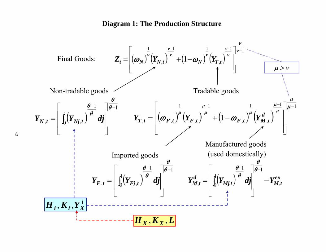
Diagram 1: The Production Structure
1
,,
1111
1
tTNtNNt YYZFinal Goods:
11
11111
Non-tradable goods Tradable goods
10 ,,
djYY tNjtN ,,,,, 1
dtMtFtFtFtT YYY
M f d d
32
Imported goods
11
Manufactured goods(used domestically)
11
10 ,,
djYY tFjtF extMtMj
dtM YdjYY ,
10 ,,
iYKH Xii YKH ,,
LKH XX ,,
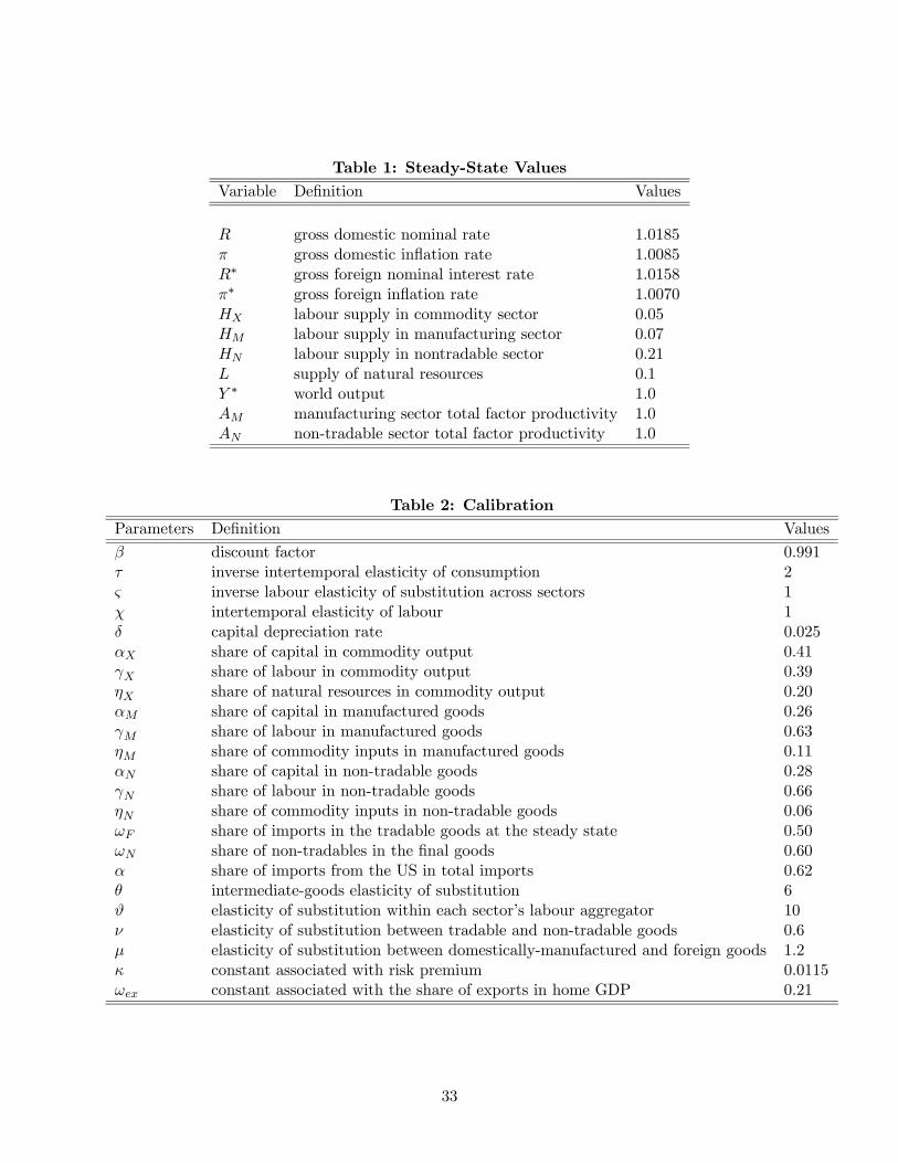
Table 1: Steady-State Values
Variable Definition Values
gross domestic nominal rate 1.0185
gross domestic inflation rate 1.0085
∗ gross foreign nominal interest rate 1.0158
∗ gross foreign inflation rate 1.0070
labour supply in commodity sector 0.05
labour supply in manufacturing sector 0.07
labour supply in nontradable sector 0.21
supply of natural resources 0.1
∗ world output 1.0
manufacturing sector total factor productivity 1.0
non-tradable sector total factor productivity 1.0
Table 2: Calibration
Parameters Definition Values
discount factor 0.991
inverse intertemporal elasticity of consumption 2
inverse labour elasticity of substitution across sectors 1
intertemporal elasticity of labour 1
capital depreciation rate 0.025
share of capital in commodity output 0.41
share of labour in commodity output 0.39
share of natural resources in commodity output 0.20
share of capital in manufactured goods 0.26
share of labour in manufactured goods 0.63
share of commodity inputs in manufactured goods 0.11
share of capital in non-tradable goods 0.28
share of labour in non-tradable goods 0.66
share of commodity inputs in non-tradable goods 0.06
share of imports in the tradable goods at the steady state 0.50
share of non-tradables in the final goods 0.60
share of imports from the US in total imports 0.62
intermediate-goods elasticity of substitution 6
elasticity of substitution within each sector’s labour aggregator 10
elasticity of substitution between tradable and non-tradable goods 0.6
elasticity of substitution between domestically-manufactured and foreign goods 1.2
constant associated with risk premium 0.0115
constant associated with the share of exports in home GDP 0.21
33
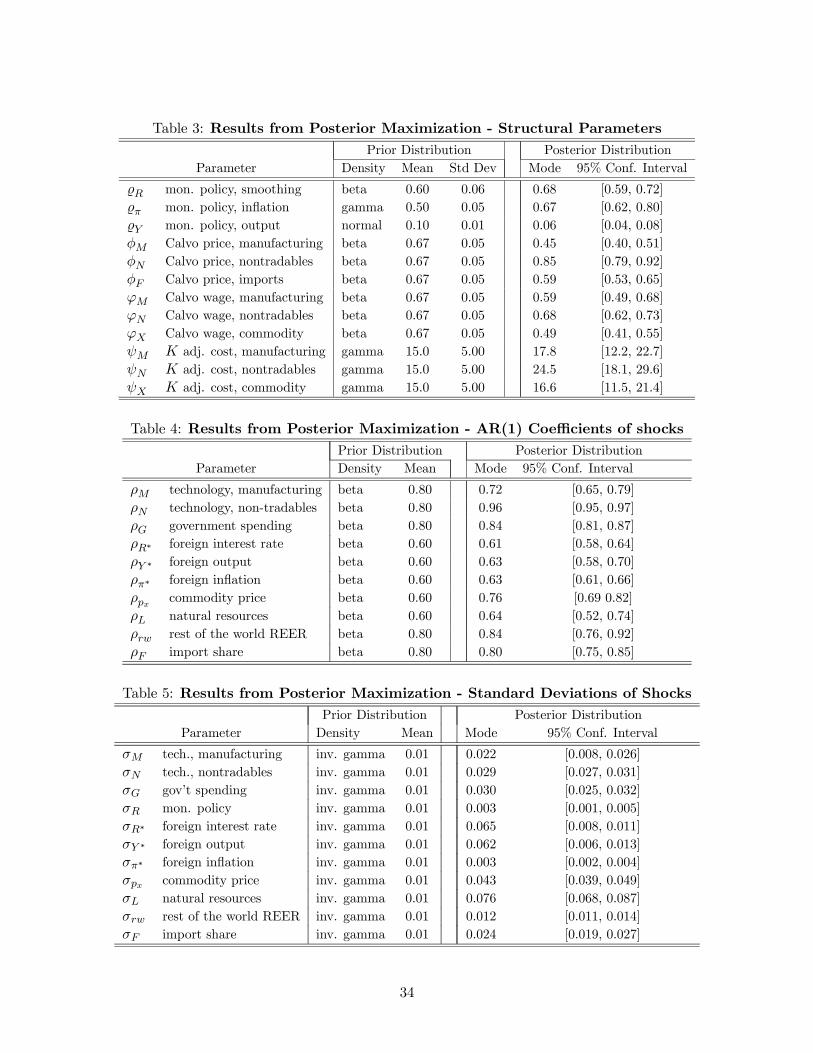
Table 3: Results from Posterior Maximization - Structural Parameters
Prior Distribution Posterior Distribution
Parameter Density Mean Std Dev Mode 95% Conf. Interval
mon. policy, smoothing beta 0.60 0.06 0.68 [0.59, 0.72]
mon. policy, inflation gamma 0.50 0.05 0.67 [0.62, 0.80]
mon. policy, output normal 0.10 0.01 0.06 [0.04, 0.08]
Calvo price, manufacturing beta 0.67 0.05 0.45 [0.40, 0.51]
Calvo price, nontradables beta 0.67 0.05 0.85 [0.79, 0.92]
Calvo price, imports beta 0.67 0.05 0.59 [0.53, 0.65]
Calvo wage, manufacturing beta 0.67 0.05 0.59 [0.49, 0.68]
Calvo wage, nontradables beta 0.67 0.05 0.68 [0.62, 0.73]
Calvo wage, commodity beta 0.67 0.05 0.49 [0.41, 0.55]
adj. cost, manufacturing gamma 15.0 5.00 17.8 [12.2, 22.7]
adj. cost, nontradables gamma 15.0 5.00 24.5 [18.1, 29.6]
adj. cost, commodity gamma 15.0 5.00 16.6 [11.5, 21.4]
Table 4: Results from Posterior Maximization - AR(1) Coefficients of shocks
Prior Distribution Posterior Distribution
Parameter Density Mean Mode 95% Conf. Interval
technology, manufacturing beta 0.80 0.72 [0.65, 0.79]
technology, non-tradables beta 0.80 0.96 [0.95, 0.97]
government spending beta 0.80 0.84 [0.81, 0.87]
∗ foreign interest rate beta 0.60 0.61 [0.58, 0.64]
∗ foreign output beta 0.60 0.63 [0.58, 0.70]
∗ foreign inflation beta 0.60 0.63 [0.61, 0.66]
commodity price beta 0.60 0.76 [0.69 0.82]
natural resources beta 0.60 0.64 [0.52, 0.74]
rest of the world REER beta 0.80 0.84 [0.76, 0.92]
import share beta 0.80 0.80 [0.75, 0.85]
Table 5: Results from Posterior Maximization - Standard Deviations of Shocks
Prior Distribution Posterior Distribution
Parameter Density Mean Mode 95% Conf. Interval
tech., manufacturing inv. gamma 0.01 0.022 [0.008, 0.026]
tech., nontradables inv. gamma 0.01 0.029 [0.027, 0.031]
gov’t spending inv. gamma 0.01 0.030 [0.025, 0.032]
mon. policy inv. gamma 0.01 0.003 [0.001, 0.005]
∗ foreign interest rate inv. gamma 0.01 0.065 [0.008, 0.011]
∗ foreign output inv. gamma 0.01 0.062 [0.006, 0.013]
∗ foreign inflation inv. gamma 0.01 0.003 [0.002, 0.004]
commodity price inv. gamma 0.01 0.043 [0.039, 0.049]
natural resources inv. gamma 0.01 0.076 [0.068, 0.087]
rest of the world REER inv. gamma 0.01 0.012 [0.011, 0.014]
import share inv. gamma 0.01 0.024 [0.019, 0.027]
34
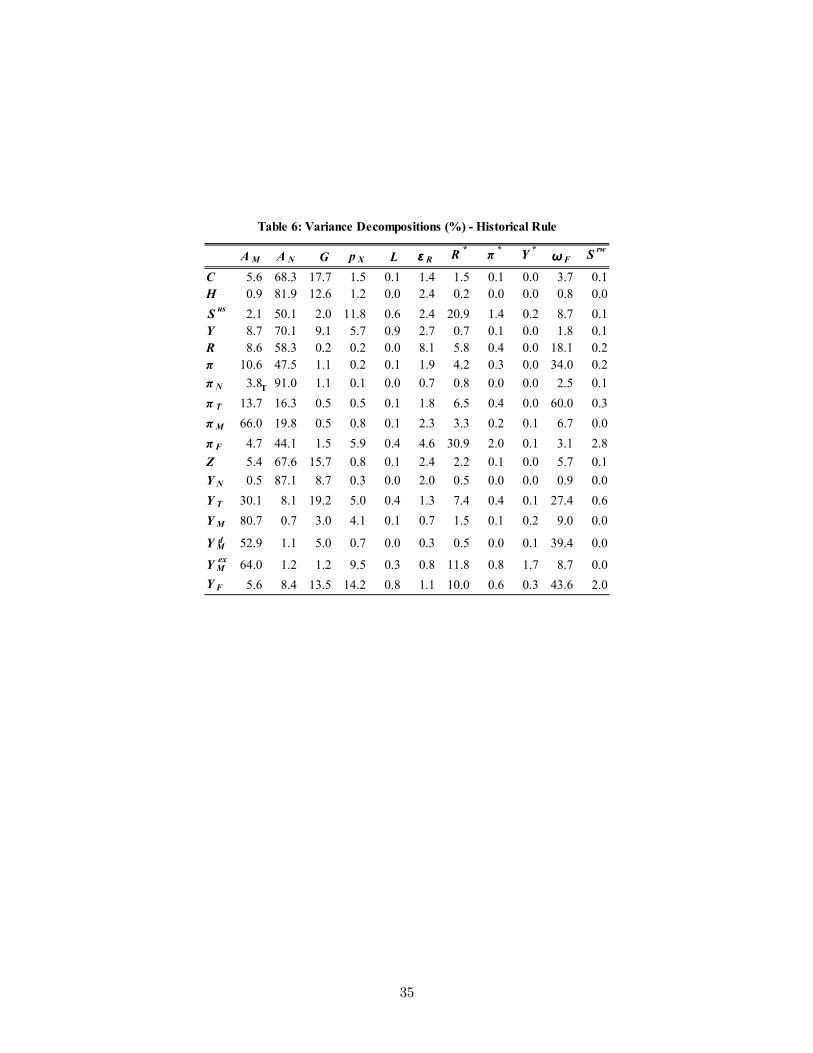
A M A N G p X L ε R R * π * Y * ω F S rw
C 5.6 68.3 17.7 1.5 0.1 1.4 1.5 0.1 0.0 3.7 0.1H 0.9 81.9 12.6 1.2 0.0 2.4 0.2 0.0 0.0 0.8 0.0S us 2.1 50.1 2.0 11.8 0.6 2.4 20.9 1.4 0.2 8.7 0.1Y 8.7 70.1 9.1 5.7 0.9 2.7 0.7 0.1 0.0 1.8 0.1R 8.6 58.3 0.2 0.2 0.0 8.1 5.8 0.4 0.0 18.1 0.2π 10.6 47.5 1.1 0.2 0.1 1.9 4.2 0.3 0.0 34.0 0.2π N 3.8 91.0 1.1 0.1 0.0 0.7 0.8 0.0 0.0 2.5 0.1π T 13.7 16.3 0.5 0.5 0.1 1.8 6.5 0.4 0.0 60.0 0.3π M 66.0 19.8 0.5 0.8 0.1 2.3 3.3 0.2 0.1 6.7 0.0π F 4.7 44.1 1.5 5.9 0.4 4.6 30.9 2.0 0.1 3.1 2.8Z 5.4 67.6 15.7 0.8 0.1 2.4 2.2 0.1 0.0 5.7 0.1Y N 0.5 87.1 8.7 0.3 0.0 2.0 0.5 0.0 0.0 0.9 0.0Y T 30.1 8.1 19.2 5.0 0.4 1.3 7.4 0.4 0.1 27.4 0.6Y M 80.7 0.7 3.0 4.1 0.1 0.7 1.5 0.1 0.2 9.0 0.0
Y M 52.9 1.1 5.0 0.7 0.0 0.3 0.5 0.0 0.1 39.4 0.0
Y M 64.0 1.2 1.2 9.5 0.3 0.8 11.8 0.8 1.7 8.7 0.0Y F 5.6 8.4 13.5 14.2 0.8 1.1 10.0 0.6 0.3 43.6 2.0
Table 6: Variance Decompositions (%) - Historical Rule
T
d
ex
35
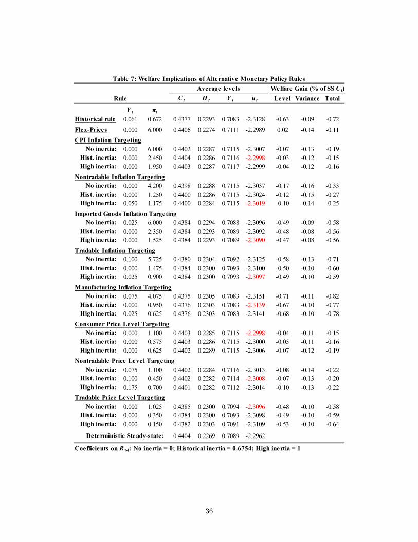
C t H t Y t u t Level Variance Total
Y t πtHistorical rule 0.061 0.672 0.4377 0.2293 0.7083 -2.3128 -0.63 -0.09 -0.72Flex-Prices 0.000 6.000 0.4406 0.2274 0.7111 -2.2989 0.02 -0.14 -0.11CPI Inflation Targeting
No inertia: 0.000 6.000 0.4402 0.2287 0.7115 -2.3007 -0.07 -0.13 -0.19Hist. inertia: 0.000 2.450 0.4404 0.2286 0.7116 -2.2998 -0.03 -0.12 -0.15High inertia: 0.000 1.950 0.4403 0.2287 0.7117 -2.2999 -0.04 -0.12 -0.16
Nontradable Inflation TargetingNo inertia: 0.000 4.200 0.4398 0.2288 0.7115 -2.3037 -0.17 -0.16 -0.33
Hist. inertia: 0.000 1.250 0.4400 0.2286 0.7115 -2.3024 -0.12 -0.15 -0.27High inertia: 0.050 1.175 0.4400 0.2284 0.7115 -2.3019 -0.10 -0.14 -0.25
Imported Goods Inflation TargetingNo inertia: 0.025 6.000 0.4384 0.2294 0.7088 -2.3096 -0.49 -0.09 -0.58
Hist. inertia: 0.000 2.350 0.4384 0.2293 0.7089 -2.3092 -0.48 -0.08 -0.56High inertia: 0.000 1.525 0.4384 0.2293 0.7089 -2.3090 -0.47 -0.08 -0.56
Tradable Inflation TargetingNo inertia: 0.100 5.725 0.4380 0.2304 0.7092 -2.3125 -0.58 -0.13 -0.71
Hist. inertia: 0.000 1.475 0.4384 0.2300 0.7093 -2.3100 -0.50 -0.10 -0.60High inertia: 0.025 0.900 0.4384 0.2300 0.7093 -2.3097 -0.49 -0.10 -0.59
Manufacturing Inflation TargetingNo inertia: 0.075 4.075 0.4375 0.2305 0.7083 -2.3151 -0.71 -0.11 -0.82
Hist. inertia: 0.000 0.950 0.4376 0.2303 0.7083 -2.3139 -0.67 -0.10 -0.77High inertia: 0.025 0.625 0.4376 0.2303 0.7083 -2.3141 -0.68 -0.10 -0.78
Consumer Price Level TargetingNo inertia: 0.000 1.100 0.4403 0.2285 0.7115 -2.2998 -0.04 -0.11 -0.15
Hist. inertia: 0.000 0.575 0.4403 0.2286 0.7115 -2.3000 -0.05 -0.11 -0.16High inertia: 0.000 0.625 0.4402 0.2289 0.7115 -2.3006 -0.07 -0.12 -0.19
Nontradable Price Level TargetingNo inertia: 0.075 1.100 0.4402 0.2284 0.7116 -2.3013 -0.08 -0.14 -0.22
Hist. inertia: 0.100 0.450 0.4402 0.2282 0.7114 -2.3008 -0.07 -0.13 -0.20High inertia: 0.175 0.700 0.4401 0.2282 0.7112 -2.3014 -0.10 -0.13 -0.22
Tradable Price Level TargetingNo inertia: 0.000 1.025 0.4385 0.2300 0.7094 -2.3096 -0.48 -0.10 -0.58
Hist. inertia: 0.000 0.350 0.4384 0.2300 0.7093 -2.3098 -0.49 -0.10 -0.59High inertia: 0.000 0.150 0.4382 0.2303 0.7091 -2.3109 -0.53 -0.10 -0.64
Deterministic Steady-state: 0.4404 0.2269 0.7089 -2.2962
Coefficients on R t-1: No inertia = 0; Historical inertia = 0.6754; High inertia = 1
Rule
Table 7: Welfare Implications of Alternative Monetary Policy Rules
Average levels Welfare Gain (% of SS C t)
36
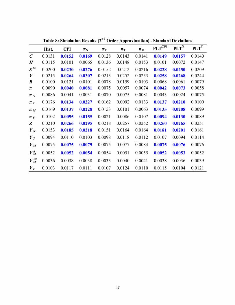
Hist. CPI πN πF πT πM PLTCPI PLTN PLTT
C 0.0131 0.0152 0.0169 0.0128 0.0143 0.0141 0.0149 0.0157 0.0140H 0.0115 0.0101 0.0065 0.0136 0.0148 0.0153 0.0101 0.0072 0.0147S us 0.0200 0.0230 0.0276 0.0152 0.0212 0.0216 0.0228 0.0250 0.0209Y 0.0215 0.0264 0.0307 0.0213 0.0252 0.0253 0.0258 0.0268 0.0244R 0.0100 0.0121 0.0101 0.0078 0.0159 0.0103 0.0068 0.0061 0.0079π 0.0090 0.0040 0.0081 0.0075 0.0057 0.0074 0.0042 0.0073 0.0058π N 0.0086 0.0041 0.0031 0.0070 0.0075 0.0081 0.0043 0.0024 0.0075π T 0.0176 0.0134 0.0227 0.0162 0.0092 0.0133 0.0137 0.0210 0.0100π M 0.0169 0.0137 0.0228 0.0153 0.0101 0.0063 0.0135 0.0208 0.0099π F 0.0102 0.0095 0.0155 0.0021 0.0086 0.0107 0.0094 0.0130 0.0089Z 0.0210 0.0266 0.0295 0.0218 0.0257 0.0252 0.0260 0.0265 0.0251Y N 0.0153 0.0185 0.0218 0.0151 0.0164 0.0164 0.0181 0.0201 0.0161Y T 0.0094 0.0110 0.0103 0.0098 0.0118 0.0112 0.0107 0.0094 0.0114Y M 0.0075 0.0075 0.0079 0.0075 0.0077 0.0084 0.0075 0.0076 0.0076
Y M 0.0052 0.0052 0.0054 0.0054 0.0051 0.0055 0.0052 0.0053 0.0052
Y M 0.0036 0.0038 0.0038 0.0033 0.0040 0.0041 0.0038 0.0036 0.0039Y F 0.0103 0.0117 0.0111 0.0107 0.0124 0.0110 0.0115 0.0104 0.0121
Table 8: Simulation Results (2nd Order Approximation) - Standard Deviations
d
ex
37
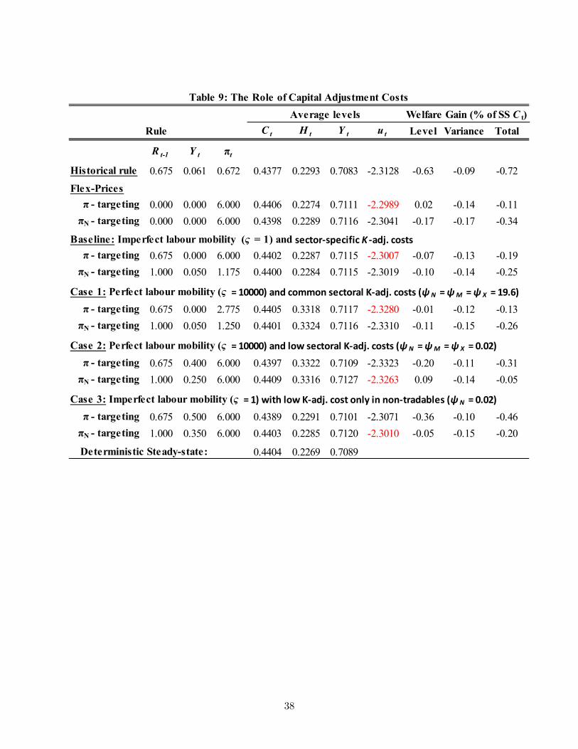
C t H t Y t u t Level Variance Total
R t-1 Y t πt
Historical rule 0.675 0.061 0.672 0.4377 0.2293 0.7083 -2.3128 -0.63 -0.09 -0.72Flex-Prices
π - targeting 0.000 0.000 6.000 0.4406 0.2274 0.7111 -2.2989 0.02 -0.14 -0.11πN - targeting 0.000 0.000 6.000 0.4398 0.2289 0.7116 -2.3041 -0.17 -0.17 -0.34
Baseline: Imperfect labour mobility (ς = 1) and sector‐specific K ‐adj. costs
π - targeting 0.675 0.000 6.000 0.4402 0.2287 0.7115 -2.3007 -0.07 -0.13 -0.19πN - targeting 1.000 0.050 1.175 0.4400 0.2284 0.7115 -2.3019 -0.10 -0.14 -0.25
Case 1: Perfect labour mobility (ς = 10000) and common sectoral K‐adj. costs (ψN = ψM = ψ X = 19.6)
π - targeting 0.675 0.000 2.775 0.4405 0.3318 0.7117 -2.3280 -0.01 -0.12 -0.13πN - targeting 1.000 0.050 1.250 0.4401 0.3324 0.7116 -2.3310 -0.11 -0.15 -0.26
Case 2: Perfect labour mobility (ς = 10000) and low sectoral K‐adj. costs (ψN = ψM = ψ X = 0.02)
π - targeting 0.675 0.400 6.000 0.4397 0.3322 0.7109 -2.3323 -0.20 -0.11 -0.31πN - targeting 1.000 0.250 6.000 0.4409 0.3316 0.7127 -2.3263 0.09 -0.14 -0.05
Case 3: Imperfect labour mobility (ς = 1) with low K‐adj. cost only in non‐tradables (ψN = 0.02)
π - targeting 0.675 0.500 6.000 0.4389 0.2291 0.7101 -2.3071 -0.36 -0.10 -0.46πN - targeting 1.000 0.350 6.000 0.4403 0.2285 0.7120 -2.3010 -0.05 -0.15 -0.20
Deterministic Steady-state: 0.4404 0.2269 0.7089
Table 9: The Role of Capital Adjustment Costs
Average levels Welfare Gain (% of SS C t)
Rule
38
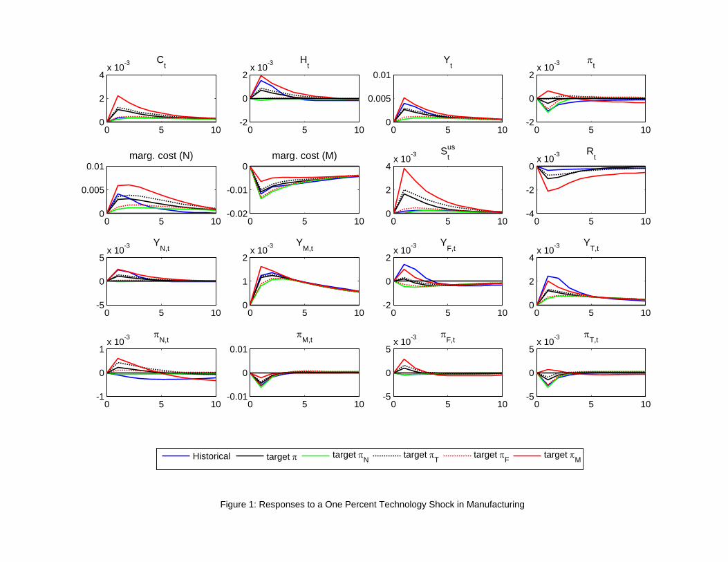
0 5 100
2
4x 10⁻³ C
t
0 5 10-2
0
2x 10⁻³ H
t
0 5 100
0.005
0.01Y
t
0 5 10-2
0
2x 10⁻³
t
0 5 100
0.005
0.01marg. cost (N)
0 5 10-0.02
-0.01
0marg. cost (M)
0 5 100
2
4x 10⁻³ Sus
t
0 5 10-4
-2
0x 10-3 R
t
0 5 10-5
0
5x 10⁻³ Y
N,t
0 5 100
1
2x 10⁻³ Y
M,t
0 5 10-2
0
2x 10⁻³ Y
F,t
0 5 100
2
4x 10⁻³ Y
T,t
0 5 10-1
0
1x 10⁻³
N,t
0 5 10-0.01
0
0.01
M,t
0 5 10-5
0
5x 10⁻³
F,t
0 5 10-5
0
5x 10⁻³
T,t
Historical target target N target T target F target M
Figure 1: Responses to a One Percent Technology Shock in Manufacturing
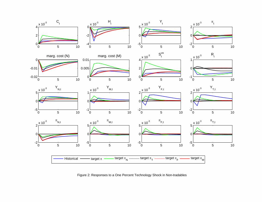
0 5 100
2
4x 10⁻³ C
t
0 5 10-4
-2
0x 10-3 H
t
0 5 10-5
0
5x 10⁻³ Y
t
0 5 10-2
0
2x 10⁻³
t
0 5 10-0.02
-0.01
0marg. cost (N)
0 5 100
0.005
0.01marg. cost (M)
0 5 100
2
4x 10⁻³ Sus
t
0 5 10-1
0
1x 10⁻³ R
t
0 5 10-5
0
5x 10⁻³ Y
N,t
0 5 10-1
0
1x 10⁻³ Y
M,t
0 5 10-2
0
2x 10⁻³ Y
F,t
0 5 10-2
0
2x 10⁻³ Y
T,t
0 5 10-2
0
2x 10⁻³
N,t
0 5 10-5
0
5x 10⁻³
M,t
0 5 10-5
0
5x 10⁻³
F,t
0 5 10-5
0
5x 10⁻³
T,t
Historical target target N target T target F target M
Figure 2: Responses to a One Percent Technology Shock in Non-tradables
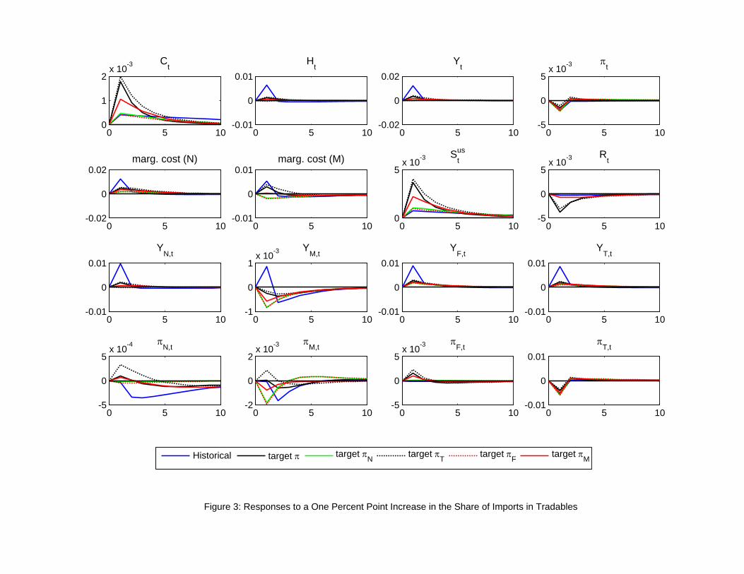
0 5 100
1
2x 10⁻³ C
t
0 5 10-0.01
0
0.01H
t
0 5 10-0.02
0
0.02Y
t
0 5 10-5
0
5x 10⁻³
t
0 5 10-0.02
0
0.02marg. cost (N)
0 5 10-0.01
0
0.01marg. cost (M)
0 5 100
5x 10⁻³ Sus
t
0 5 10-5
0
5x 10⁻³ R
t
0 5 10-0.01
0
0.01Y
N,t
0 5 10-1
0
1x 10⁻³ Y
M,t
0 5 10-0.01
0
0.01Y
F,t
0 5 10-0.01
0
0.01Y
T,t
0 5 10-5
0
5x 10⁻⁴
N,t
0 5 10-2
0
2x 10⁻³
M,t
0 5 10-5
0
5x 10⁻³
F,t
0 5 10-0.01
0
0.01
T,t
Historical target target N target T target F target M
Figure 3: Responses to a One Percent Point Increase in the Share of Imports in Tradables

0 5 100
0.5
1x 10⁻³ C
t
0 5 10-1
0
1x 10⁻³ H
t
0 5 100
1
2x 10⁻³ Y
t
0 5 10-5
0
5x 10⁻⁴
t
0 5 10-2
0
2x 10⁻³marg. cost (N)
0 5 10-5
0
5x 10⁻³marg. cost (M)
0 5 100
1
2x 10⁻³ Sus
t
0 5 10
-4
-2
0x 10-4 R
t
0 5 10-1
0
1x 10⁻³ Y
N,t
0 5 10-2
0
2x 10⁻⁴ Y
M,t
0 5 100
0.5
1x 10⁻³ Y
F,t
0 5 100
0.5
1x 10⁻³ Y
T,t
0 5 10-5
0
5x 10⁻⁴
N,t
0 5 10-2
0
2x 10⁻³
M,t
0 5 10-2
0
2x 10⁻³
F,t
0 5 10-1
0
1x 10⁻³
T,t
Historical target target N target T target F target M
Figure 4: Responses to a Negative One Percent Shock in the USD/RW REER
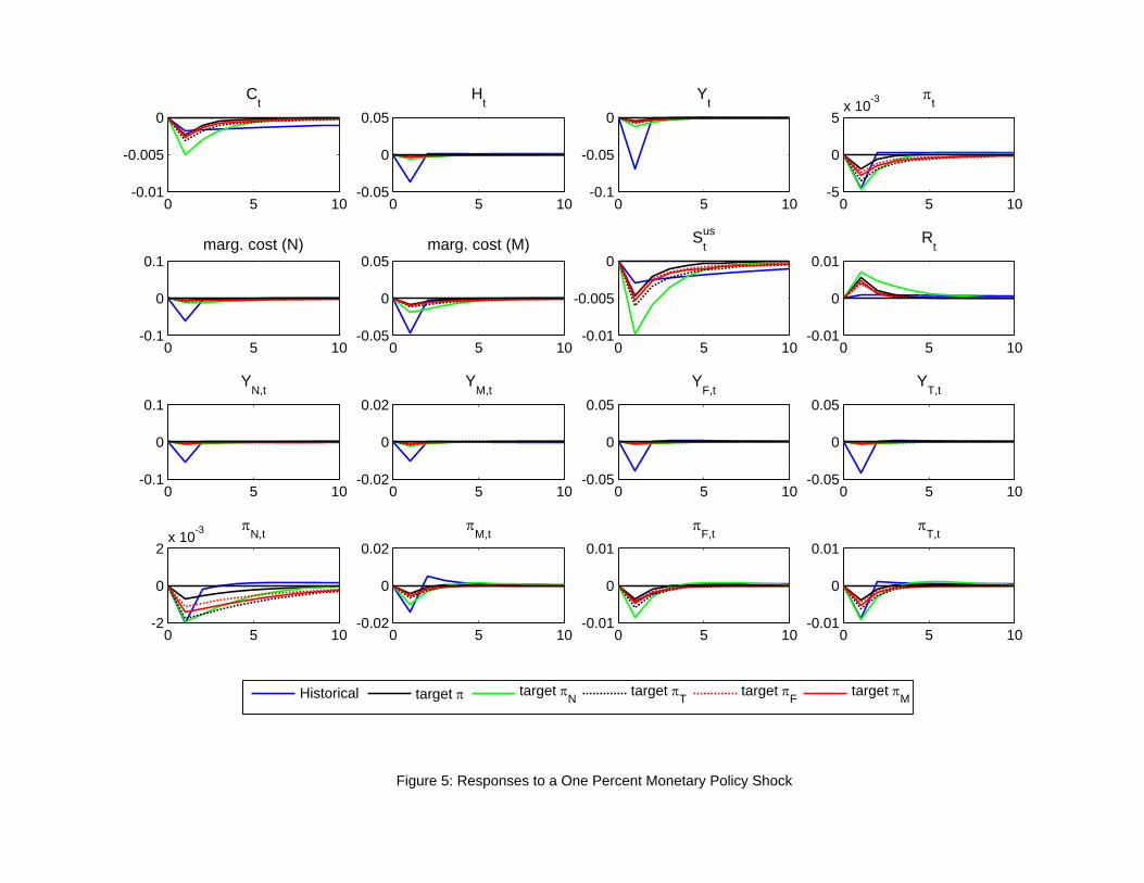
0 5 10-0.01
-0.005
0C
t
0 5 10-0.05
0
0.05H
t
0 5 10-0.1
-0.05
0Y
t
0 5 10-5
0
5x 10⁻³
t
0 5 10-0.1
0
0.1marg. cost (N)
0 5 10-0.05
0
0.05marg. cost (M)
0 5 10-0.01
-0.005
0Sus
t
0 5 10-0.01
0
0.01R
t
0 5 10-0.1
0
0.1Y
N,t
0 5 10-0.02
0
0.02Y
M,t
0 5 10-0.05
0
0.05Y
F,t
0 5 10-0.05
0
0.05Y
T,t
0 5 10-2
0
2x 10⁻³
N,t
0 5 10-0.02
0
0.02
M,t
0 5 10-0.01
0
0.01
F,t
0 5 10-0.01
0
0.01
T,t
Historical target target N target T target F target M
Figure 5: Responses to a One Percent Monetary Policy Shock

0 5 100
1
2x 10⁻³ C
t
0 5 10-5
0
5x 10⁻³ H
t
0 5 100
0.005
0.01Y
t
0 5 10-1
0
1x 10⁻³
t
0 5 10-0.01
0
0.01marg. cost (N)
0 5 10-0.02
-0.01
0marg. cost (M)
0 5 100
1
2x 10⁻³ Sus
t
0 5 10-2
-1
0x 10-3 R
t
0 5 10-5
0
5x 10⁻³ Y
N,t
0 5 100
1
2x 10⁻³ Y
M,t
0 5 10-5
0
5x 10⁻³ Y
F,t
0 5 100
2
4x 10⁻³ Y
T,t
0 5 10-5
0
5x 10⁻⁴
N,t
0 5 10-5
0
5x 10⁻³
M,t
0 5 10-1
0
1x 10⁻³
F,t
0 5 10-5
0
5x 10⁻³
T,t
baseline: target alternative: target when N = 0
Figure 6: The Role of K-Adjustment Costs for Optimal CPI-Inflation Targeting Rules IRF's to a 1% Technology Shock in the Manufacturing Sector

0 5 100
1
2x 10⁻³ C
t
0 5 10-4
-2
0x 10-3 H
t
0 5 100
2
4x 10⁻³ Y
t
0 5 10-5
0
5x 10⁻⁴
t
0 5 10-0.02
-0.01
0marg. cost (N)
0 5 100
0.005
0.01marg. cost (M)
0 5 100
1
2x 10⁻³ Sus
t
0 5 10-1
0
1x 10⁻³ R
t
0 5 100
2
4x 10⁻³ Y
N,t
0 5 100
2
4x 10⁻⁴ Y
M,t
0 5 100
0.5
1x 10⁻³ Y
F,t
0 5 100
0.5
1x 10⁻³ Y
T,t
0 5 10-2
0
2x 10⁻³
N,t
0 5 10-5
0
5x 10⁻³
M,t
0 5 10-2
0
2x 10⁻³
F,t
0 5 10-2
0
2x 10⁻³
T,t
baseline: target alternative: target when N = 0
FIgure 7: The Role of K-Adjustment Costs for Optimal CPI-Inflation Targeting Rules IRF's to a 1% Technology Shock in the Non-tradables Sector