ambiguous events and maxmin expected...

Journal of Economic Theory 134 (2007) 1–33www.elsevier.com/locate/jet

Ambiguous events and maxmin expected utility

Massimiliano Amarante∗, Emel FilizDepartment of Economics, Columbia University, 420 W 118th Street, NY 10027, USA

Received 7 December 2004; final version received 6 December 2005

Abstract

We study the properties associated to various definitions of ambiguity [L.G. Epstein, J. Zhang, Subjectiveprobabilities on subjectively unambiguous events, Econometrica 69 (2001) 265–306; P. Ghirardato et al.,Differentiating ambiguity and ambiguity attitude, J. Econ. Theory 118 (2004) 133–173; K. Nehring, Ca-pacities and probabilistic beliefs: a precarious coexistence, Math. Soc. Sci. 38 (1999) 197–213; J. Zhang,Subjective, ambiguity, expected utility and Choquet expected utility, Econ. Theory 20 (2002) 159–181]in the context of Maximin Expected Utility (MEU). We show that each definition of unambiguous eventsproduces certain restrictions on the set of priors, and completely characterize each definition in terms ofthe properties it imposes on the MEU functional. We apply our results to two open problems. First, in thecontext of MEU, we show the existence of a fundamental incompatibility between the axiom of “Smallunambiguous event continuity” (Epstein and Zhang, 2001) and the notions of unambiguous event due toZhang (2002) and Epstein and Zhang (2001). Second, we show that, in the context of MEU, the classes ofunambiguous events according to either Zhang (2002) or Epstein and Zhang (2001) are always �-systems.Finally, we reconsider the various definitions in light of our findings, and identify some new objects (Z-filtersand EZ-filters) corresponding to properties which, while neglected in the current literature, seem relevantto us.© 2006 Elsevier Inc. All rights reserved.

JEL classification: D81

Keywords: Ambiguous events; Maxmin expected utility

1. Introduction

The idea of Ambiguity has been central to the research in decision theory for several decades.The story is well-known. On one hand, Savage’s theory [20] postulates that a decision maker be

∗ Corresponding author.E-mail addresses: [email protected] (M. Amarante), [email protected] (E. Filiz).

0022-0531/$ - see front matter © 2006 Elsevier Inc. All rights reserved.doi:10.1016/j.jet.2005.12.009

http://www.elsevier.com/locate/jet

mailto:[email protected]

mailto:[email protected]

2 M. Amarante, E. Filiz / Journal of Economic Theory 134 (2007) 1–33

able to assign probabilities to all events. On the other hand, it is hard to dismiss the intuitionthat in many situations the information available to the decision maker might be insufficient fordoing so. Roughly speaking, “Ambiguity” refers to these situations, and the classic experimentsby Ellsberg [6] have convincingly demonstrated its empirical relevance.

The conflict featuring Savage’s theory on one side and the idea of Ambiguity on the other, hasgenerated spectacular theoretical developments: Choquet expected utility [21], maxmin expectedutility (henceforth, MEU) [10] and several generalizations of the latter [8,14,16]. All these modelsallow for modes of behavior that are not necessarily consistent with Savage’s Subjective ExpectedUtility theory. In particular, they can accommodate behavior of the type observed by Ellsberg.Yet, in most of this work, the idea of Ambiguity has remained in the background: more like aninspirational muse rather than a central, fully spelled out concept.

The formalization of the concept of Ambiguity is a more recent matter, mostly of the pastdecade. Since the idea refers to situations where not all events are assigned probabilities, the goalhas been that of characterizing such events. These are called ambiguous, and all the others arecalled unambiguous. As of today, several definitions have been proposed, amended, criticized andthe literature, in spite of its recent start, is already quite sizeable. We refer the reader to [7,8] forsome of the history of the problem.

This wealth of definitions as well as the richness of the debate surrounding them (see, forinstance, [7–9,13,15,17–19,22]) motivate the present work. Our goal is to contribute to the debateby providing a new way of looking at the problem. We do so by studying the properties associatedto various definitions of ambiguity within the context of a familiar model like MEU. The noveltyof our approach consists in the realization that the demand that a certain event be unambiguous isequivalent to the demand that the MEU functional—and, hence, the set of priors—display certainproperties. As different definitions of “ambiguous event” lead to different properties, one achievesa better understanding of those very definitions. All the more, the focus of the debate can shifttoward the desirability of these properties.

Our results admit a dual reading. Let x be a certain definition of Ambiguous event, and let T bean event. Our results say that T is x-unambiguous if and only if the MEU functional displays acertain property. Alternatively, one can view our results as follows. Let {Ai} be a certain collectionof events that are called at the outset as x-unambiguous. Then, our study shows (a) whether ornot there exists a MEU model compatible with this situation; and, in the affirmative case, that (b)the set of priors defining the MEU functional must have a certain form. The latter case can beaxiomatized by introducing an additional axiom in the familiar MEU setting.

The paper proceeds as follows: Section 2 states and motivates the assumptions that we maintainthroughout the paper. Section 3 reviews the various definitions of Ambiguity we consider. Section4 focuses on the notions proposed by Nehring [17] and Ghirardato et al. [8], while Section 5on those proposed by Zhang [22] and Epstein and Zhang [7]. As mentioned above, the unifyingtheme is the realization that an event is x-unambiguous if and only if the set of priors (andhence the maxmin functional) displays a certain structure. In Section 6, we apply our results tostudy two open problems. The first regards the axiom of “Small unambiguous event continuity”introduced in [7]. The desirability of the axiom, which is crucial for the derivation of a uniqueprobability measure on the classes of Zhang and Epstein–Zhang unambiguous events, has recentlybeen questioned (see, in particular [15,19]). In the context of MEU, our main result states theexistence of a fundamental incompatibility between this axiom and the notions of unambiguousevent due to Zhang and Epstein–Zhang. The second problem regards the properties of the classesof unambiguous events according to [7,22], respectively. Both classes were originally claimedto be �-systems. Later, Kopylov [15] showed that, in general, they are only mosaics (a notion

M. Amarante, E. Filiz / Journal of Economic Theory 134 (2007) 1–33 3

he introduced). Yet, the problem of what conditions guarantee that those classes are, in addition,�-systems has been left open. Here, we show that, in the context of MEU, those classes are indeed�-systems. Finally (Section 7), we reconsider the various definitions of ambiguity in light ofour findings, and identify some new objects (Z-filters and EZ-filters) corresponding to propertieswhich, while neglected in the current literature, seem relevant to us. Proofs are in appendix.Section A.* in appendix refers to material contained in Section * in the main text.

2. Setting

Throughout the paper, S denotes the state space, � is a �-algebra of events in S and Y is theprize space, which we assume is a mixture space [4,10]. The set of acts is F = {f : S → Y | f issimple and �-measurable}, with generic elements f, g, h, . . . , etc.

Our goal is to achieve a deeper understanding of the meaning of various definitions of ambiguousevent proposed in the literature. Studying the properties of unambiguous events in the context ofa well-understood model like MEU seems to us one but an obvious step in this direction. Thismotivates our first assumption:

Assumption 1 (MEU preferences, Gilboa and Schmeidler [10]). The decision maker’s prefer-ence relation, �, on F is represented by the functional I : F → R defined by

I (f ) = minP∈C

∫S

u(f (s)) dP(s), (1)

where C is a convex and weak*-compact set of finitely additive probability measures on (S, �),and u : Y → R is a linear utility on the prize space.

We recall that the utility function u produces an embedding of the acts into the set B0(�)

of bounded real-valued simple functions on S, and the functional I (and, hence, the preferencerelation) is extended to the whole B0(�) in the obvious way [10]. Because of this, from now on wedrop any reference to the utility function (that is, from now on an act f if viewed as a real-valuedfunction).

In pursuing our goal, we need to avoid spurious differences which might emerge solely as aconsequence of the model we are using. In their work, both Zhang [22] and Epstein–Zhang [7]assume a rich setting, which leads to the existence of a countably additive, non-atomic probabilitymeasure on the class of unambiguous events. For other definitions, like Nehring’s or Ghirardato–Maccheroni–Marinacci’s, this is possible—in the context of MEU—only if all the priors are bothcountably additive and non-atomic, and only if the class of unambiguous events is sufficientlyrich. This consideration motivates the remaining three assumptions.

Assumption 2. All the priors in C are countably additive.

Assumption 3. All the priors in C are non-atomic.

Axioms on the decision maker’s preference relation leading to the properties stated in As-sumptions 2 and 3 have been recently identified by Chateauneuf–Maccheroni–Marinacci–Tallon[4], to which we refer the reader. The final assumption, which delivers the richness of the classof unambiguous events either in the sense of Nehring or Ghirardato–Maccheroni–Marinacci,requires a bit of preparation. By Assumption 2, there exists a prior, � ∈ C, with respect to


which all the other priors in C are absolutely continuous [4, Lemma 3]. Hence, for each priorthere exists a density (with respect to �) and the set C is isometrically isomorphic to a setD ⊂ L1(S, �, �). For A ∈ � and with Ac denoting the complement of A, let D⊥(A) ={� ∈ L∞(S, �, �) | � = 0 a.e on Ac and

∫g� d� = 0 for all g ∈ D}.

Definition 1 (see Kingman and Robertson [12]). D is said to be thin if and only if D⊥(A) isdifferent from the zero subspace whenever �(A) > 0. We also say that a set of priors C is thin ifthe corresponding set of densities is.

We can now state our final assumption:

Assumption 4. The set C is thin.

Assumption 4 guarantees that the definitions of Ambiguity we are going to study are, indeed,comparable. In the context of Assumptions 1–3, it was shown in [2] (Proposition 4) that there existsa countably additive, non-atomic probability measure on the class of Ghirardato–Maccheroni–Marinacci (equivalently, Nehring’s) unambiguous events if and only if Assumption 4 is satisfied.In order to get a better grasp of how restrictive Assumption 4 is, we remark that every finite-dimensional set of non-atomic priors (i.e., every set of priors obtained as the convex hull of afinite number of priors) is thin. Thin sets, however, need not be finite-dimensional: as an example,let {An}n∈N be a countable partition of the state space S and let {Pn}n∈N be a collection of non-atomic priors with Pn supported by An for each n ∈ N. Then, it is easily seen that {Pn} (and,hence co {Pn}) is thin and infinite-dimensional. 1

3. Definitions of ambiguous events

We distinguish between two groups of definitions of ambiguous event. One group features thedefinitions given by Nehring [17] and Ghirardato et al. [8], the other those given by Zhang [22]and Epstein and Zhang [7]. In the context of Multiple Prior models, the definitions of ambiguousevent given by Nehring and Ghirardato, Maccheroni and Marinacci are known to be equivalent,and correspond to the following

Definition 2. An event T ∈ � is unambiguous if ∀P, Q ∈ C, P(T ) = Q(T ). Otherwise it isambiguous.

We borrow from Dubins and Margolis [5], 2 and we call naturally measurable all eventswhich satisfy Definition 2. The class of naturally measurable events is denoted by ANM. It is astraightforward consequence of the definition that the class ANM is a �-system [8]; in particular,it is closed under the operation of taking complements. Under Assumption 4, it contains eventsof measure �, for any � ∈ [0, 1] (see [2]; this measure is univocally defined because of the verynature of naturally measurable events).

1 Matter of fact, infinite-dimensional thin sets of priors abound. It is an easy consequence of a theorem of Kadec andPelczynski [11, Theorem 6] that every infinite-dimensional, non-reflexive subspace of L1 contains an infinite-dimensionalset, which is thin.

2 While introduced in a different context, the terminology seems especially suited to us (see [5]).


Let f be a function on S and w be a real number (recall that acts have been identified to real-valued functions), we denote by f T w the real-valued function on S which coincides with f on Tand is identically equal to w on T c. Naturally measurable events admit the following behavioralcharacterization, which is proven in [8].

Proposition 1 (Ghirardato et al. [8]). T is naturally measurable if and only if for any f, g ∈ F ,w, w′ ∈ R and for any � ∈ (0, 1)

f ∼ g �⇒ �f + (1 − �)(wT w′) ∼ �g + (1 − �)(wT w′).

The next two definitions are stated directly in behavioral terms. The definition proposed byZhang [22] reads as follows.

Definition 3. An event T ∈ � is Z-unambiguous if ∀f, g ∈ F , w ∈ R

f T w�gT w �⇒ f T w′�gT w′ for any w′ ∈ R (2)

and the same implication holds for T c. Otherwise T is Z-ambiguous.

The definition given in Epstein–Zhang [7] displays a similar structure but it is weaker in thatlimits the comparison (2) only to a certain subset of F × F . For T ∈ �, let A and B be twodisjoint subsets of T. Consider an act of the form f = [y∗, A; y, B; z(s), (A ∪ B)c], where thenotation means that f takes value y∗ on A, y on B and is equal to a function z(·) on (A ∪ B)c. AnEZ-conjugate of f is an act f = [y, A; y∗, B; z(s), (A ∪ B)c], that is, f is obtained from f byexchanging the prizes on A and B. The definition given in Epstein and Zhang reads as follows.

Definition 4. An event T ∈ � is EZ-unambiguous if ∀f ∈ F , w ∈ R and for any conjugate f

of f

f T w�f T w �⇒ f T w′�f T w′ for any w′ ∈ R

and the same implication holds for T c. Otherwise T is EZ-ambiguous.

The restriction to comparisons involving only conjugate acts is motivated by the intuition thatan event T should be called unambiguous if (and only if) the relative conditional likelihood of anytwo of its subevents, A and B, is invariant with respect to changes in the prize on T c (see [7]). Theclasses of unambiguous events according to Zhang and Epstein–Zhang are denoted by AZ andAEZ, respectively. These two notions of ambiguity have been recently discussed by Kopylov [15],who shows, among other results, that the two classes are mosaics and that they are not necessarily�-systems.

At any rate, in the setting we study, there is an obvious relation among the three notions, whichwe state in the next proposition.

Proposition 2. ANM ⊆ AZ ⊆ AEZ.

As these inclusions come straight from the definitions, we do not provide a proof (however,many of the results we present later implicitly contain a proof of this fact). Under our assumptions,the inclusion ANM ⊆ AZ may be strict as illustrated by the following example.


Example 1 (Nehring [19]). Fix an event T ∈ �. Let �1 and �2 denote two weak*-closed andconvex sets of finitely additive probability measures supported by T and T c, respectively. Fix �,� such that 0 < � < � < 1. Define the weak*-closed and convex set � as follows:

� ≡ [�, �]�1 + [1 − �, 1 − �]�2 ≡ {�1 + (1 − �)2|��, 1 ∈ �1, 2 ∈ �2}and let the preference � be the one induced by � according to the MEU functional (1).

The reader can readily check that T is Z-unambiguous, and hence EZ-unambiguous, but notnaturally measurable because � �= �. As we shall see (Theorem 4), the example goes a long waybeyond showing that the inclusion ANM ⊆ AZ is strict. In fact, it provides remarkable insightsinto the structure of events which are unambiguous either according to Zhang or to Epstein andZhang.

4. Naturally measurable events

The main result of this section (Theorem 1) states the existence of a certain relation betweennaturally measurable events and the structure of the set C, which defines the MEU functional.Precisely, if � = {Ti}ni=1 is a finite partition of S into naturally measurable events, then C can bewritten as a unique convex combination of a collection of sets {CTi

}Ti∈�, C = ∑qiCTi

, and eachmeasure in CTi

is supported by Ti . Equivalently, given a partition into naturally measurable events,the set C can be decomposed into a (canonical) system of sets of conditional measures. Later inthis section and more thoroughly in Section 7, we will elaborate on the interpretation attached tothis type of decomposition. For future reference, notice that in the special case � = {T , T c} ourresult says that to each naturally measurable event there is associated a certain decomposition ofthe set of priors and, hence, a special form of the MEU functional I.

Let � = {Ti}ni=1 be a finite partition of S with the property that each Ti ∈ ANM. For any n ∈ N,existence of such partitions is guaranteed by Assumption 4 of Section 2 (see [2]).

Theorem 1. There exist (a) a unique collection of non-empty, weak� compact, and convex setsof priors {CTi

}Ti∈�, where for any Ti ∈ �, CTi⊆ {P | P is a probability measure on Ti}; and (b)

a unique probability distribution q = (q1, . . . , qn) such that for any f ∈ F

minP∈C

∫S

f dP = I (f ) =n∑

i=1

(min

P∈CTi

∫Ti

f dP

)qi,

where qi = P(Ti), i = 1, . . . , n, for all P ∈ C. 3

We stress that the decomposition of Theorem 1 holds for any act f ∈ F . With this in mind,Theorem 1 lends itself to an interesting interpretation. We can think of a MEU decision makeras of someone who follows a two-step procedure. In the first step, acts are decomposed into acollection of subacts each defined on a naturally measurable event. No ambiguity is attached toany of these events and each subact is evaluated by means of a MEU functional. In the second step,all these evaluations are aggregated linearly by means of q. Theorem 1 has an obvious converse(whose proof is immediate), which we will use later (see Theorem 4):

3 Under the assumption that the partition is measurable, one can easily extend Theorem 1 to the case of uncountablepartitions.


Proposition 3. Let {Ti}ni=1 be a partition of S, and, for each i, let CTi⊆ {P | P is a probability

measure on Ti}. If C = ∑ni=1 qiCTi

, qi �0 and∑n

i=1 qi = 1, then each Ti is naturally measurable.

5. Zhang and Epstein–Zhang unambiguous events

In this section, we study Zhang and Epstein–Zhang unambiguous events. We restrict attentionto acts of the form f T w (and f T cw) since both Zhang and Epstein–Zhang consider only actshaving this form. Throughout the section, T is a fixed event and we use the notation f (w) in theplace of f T w. The rationale for this notational change will be clear in Section 5.2, below. Werestrict to events T such that 0 < min P(T )� max P(T ) < 1 because if T is such that eithermin P(T ) = 0 and max P(T ) �= 0 or min P(T ) �= 1 and max P(T ) = 1, then T is necessarilyEZ-ambiguous (see Appendix, Proposition 6). Finally, to simplify the exposition, we henceforthcall Z/EZ unambiguous events those events T that satisfy only the first half of the original definition(for example: T is Z-unambiguous if it satisfies Eq. (2) without the symmetric requirement forT c). This simplification is harmless: since both definitions consist of two separate parts, one getsa complete necessary/sufficient condition by simply requiring that the same condition be satisfiedwhen one exchanges T with its complement T c.

Our analysis unfolds as follows. We begin by observing that the study of unambiguous events isintimately related to that of certain functionals. This point of view turns out to be extremely useful.At once, we are able to give a useful necessary condition for an event to be Z-unambiguous (Section5.1), and to show that the problem we are concerned with lends itself to a simple geometricaldescription (Section 5.2). The first two Subsections prepare the ground for the two main results ofthe section. In Section 5.3, we give a complete characterization of Z-unambiguous events, whilein Section 5.4 we show the equivalence between Zhang’s and Epstein–Zhang’s definitions.

5.1. From naturally measurable events to Zhang unambiguous events

In light of the inclusion ANM ⊆ AZ (Proposition 2), we are concerned with finding andcharacterizing those Zhang unambiguous events (if any) which are not naturally measurable. Ouranalysis takes off from the following considerations. Consider the two subsets of priors

CMIN = arg minP∈C

P(T ) and CMAX = arg maxP∈C

P(T ).

Clearly, both CMAX and CMIN are non-empty, convex and weak*-compact. Moreover, it is imme-diate to verify that either CMAX ∩ CMIN = ∅ or CMAX = CMIN = C. By using the sets CMAX and

CMIN, we can define two functionals, I and≈I , by

I (f ) = minCMAX

∫f dP,

≈I (f ) = min

CMIN

∫f dP.

The main reason for introducing I and≈I is that (as the reader can easily check) the ranking they

induce on acts of the form f (w) is independent of w. That is,

I (f (w)) � I (g(w)) for some w �⇒ I (f (w′))� I (g(w′)) ∀w′ ∈ R,≈I (f (w)) �

≈I (g(w)) for some w �⇒ ≈

I (f (w′))�≈I (g(w′)) ∀w′ ∈ R.


For brevity, we will refer to this property as to w-invariance. The functionals I and≈I provide us

with another way to look at naturally measurable events. For if T is naturally measurable, then

CMAX = CMIN = C and for any act f, we have I (f ) = I (f ) = ≈I (f ). Hence, the unambiguous

nature of T follows at once from the observed w-invariance Incidentally, this also shows theinclusion ANM ⊆ AZ.

If T is not naturally measurable, the functional I which evaluates the acts is, in general, different

from both I and≈I . The next lemma, however, shows that for any act f there exists a f (w∗)

[f (w∗∗)] for which I (f (w∗)) = ≈I (f (w∗)) [I (f (w∗∗)) = I (f (w∗∗))]. Equivalently, such an act

is evaluated by a prior in CMIN [CMAX].

Lemma 1. For any act of the type f (w),

(a) ∃w∗ such that I (f (w)) = ≈I (f (w)) for any w�w∗;

(b) ∃w∗∗ such that I (f (w)) = I (f (w)) for any w�w∗∗.

Lemma 1 is a basic result in our analysis as it immediately leads to uncover a number ofproperties associated with Zhang unambiguous events. In fact, by combining Lemma 1 with the

w-invariance of I and≈I , we obtain at once the following necessary condition for T ∈ AZ.

Proposition 4. A necessary condition for T ∈ AZ is that if f (w′)�g(w′) at some w′, then both≈I (f (w′)) �

≈I (g(w′)),

I (f (w′)) � I (g(w′)).

While the proof is in the appendix, the reader might want to defer its reading until next sub-section, where we give a simple geometric explanation of the content of Proposition 4 (Fig. 2).

5.2. A geometric analysis

The concepts we have seen so far lend themselves to a very simple geometric description. In

fact, due to the restriction to acts of the form f (w), the functionals I, I and≈I implicitly define

certain families of real functions of real variable. For f of the type f (w), define If : R → R byIf (w) = I (f (w)).

Proposition 5. For any f = f (w), If is (a) increasing; (b) concave and (c) continuous.

In a similar fashion, by using the functionals I and≈I in the place of I, we define the functions If

and≈I f , which are straight lines with slopes 1 − Pmax(T ) and 1 − Pmin(T ), respectively. Finally,

let

If (w) = If (w) ∧ ≈I f (w) = min

{If (w),

≈I f (w)

}.

The latter functions will play a major role in our analysis. Fig. 1 below describes all the functionscorresponding to a given f as well as the content of Lemma 1.


Fig. 1. For w�w∗f, If = ≈

If while for w�w∗∗, If = If . For w ∈ (w∗f, w∗∗

f), If is a concave function between

If = If ∧ ≈If and the line joining

≈If (w∗) and If (w∗∗).

Fig. 2. If Cond NC is not satisfied, the I·’s and≈I ·’s are as in the picture. Any concave If and Ig intersect at some w

leading to T �∈ AZ.

By means of this type of diagrams, we can now give a simple illustration of the necessarycondition found above. In the notation just introduced, we can concisely reformulate the contentof Proposition 4 as follows

Condition NC. If T ∈ AZ, then f (w)�g(w) at some w implies If (w)� Ig(w), ∀w (Fig. 2).

5.3. Necessary and sufficient conditions

We are now ready to give a complete characterization of Zhang unambiguous events.

Theorem 2. T ∈ AZ if and only if the following conditions are satisfied:

(i) Condition NC:∀f, g of the formf =f T w andg=gTw, either If (w)� Ig(w)or If (w)� Ig(w)

for any w ∈ R;(ii) The functional I restricted to acts of the form f T w is equal to I .

Sufficiency of the two conditions is immediate from geometrical inspection. Necessity of (i) wasshown above. Only the proof of necessity of (ii) requires a certain amount of work. Summarily,


here is how it goes: for C a set of priors, denote by C |T the set of conditional probabilitiescomputed from probabilities in C. Now, suppose that

CMIN |T ∩CMAX |T = � (3)

and consider the act 0T w (that is, the act that is identically equal to 0 on T and identicallyequal to w on T c). A separation theorem due to Amarante and Maccheroni [3] implies that thereexist two disjoint subsets, A and B, of T, such that P(A) − P(B) > 0 > Q(A) − Q(B) forany P ∈ CMIN and any Q ∈ CMAX. This suggests that, for > 0, we consider the act rT w,where r is the function r = [�A − �B ], and �A and �B are the indicator functions of A and B,respectively. The continuity properties of the MEU functional imply (see Lemma 5 in appendix)that there exists an ∗ such that for any measure R ∈ arg min

P∈CMIN

(∫(∗[�A−�B ]T w) dP), we have that

R(A)−R(B) > 0. Clearly, this implies that when both ∗[�A −�B ]T w and 0T w are evaluated bymeasures in CMIN (this certainly happens because of Lemma 1), we have ∗[�A −�B ]T w � 0T w.Analogously, when both ∗[�A − �B ]T w and 0T w are evaluated by measures in CMAX, we have∗[�A − �B ]T w ≺ 0T w. But this means that T is Zhang ambiguous. In other words, if T ∈ AZthen the intersection in (3) has to be non-empty. In the general case, for f an act of the type f T w,we consider the sets

≈�f = arg min

P∈CMIN

∫f dP; �f = arg min

P∈CMAX

∫f dP ; �f = arg min

P∈C

∫f dP

and prove the following characterization of Condition NC.

Lemma 2. Condition NC is equivalent to the condition that for any act f

(≈�f |T ) ∩ (�f |T ) �= ∅.

Next, we show (Lemma 6 in appendix) that if for some f we have If (w) < If (w), then it

must be the case that either �f |T ∩ ≈�f |T = � or �f |T ∩�f |T = �. Then, in both cases,

we can follow a procedure similar to the one outlined above to establish that T has to be Zhangambiguous. That is if T ∈ AZ, then for any f, we must have If (w) = If (w).

5.4. Epstein–Zhang unambiguous events

As general matter (Section 3), Epstein–Zhang’s definition is more permissive than Zhang’s.In fact, conditions guaranteeing that the two are non-equivalent can be derived from Epstein–Zhang’s paper, in particular Corollary 7.3. The next theorem, however, shows that the two coincideunder Assumptions 1–4.

Theorem 3. AZ = AEZ.

Details are in appendix, but the intuition is simple. For if T ∈ AZ\AEZ, at least one of theconditions in Theorem 2 must be violated, and (either case) there exist (a) acts f T w and f T w′;(b) priors P and P ′ with I (f T w) = ∫

f T w dP and I (f T w′) = ∫f T w′ dP′; and (c) events A

and B, in T such that P(A) − P(B) > 0 > P ′(A) − P ′(B) (incidentally, this would imply that


the conditional relative likelihood of A versus B varies with the act which is evaluated). Given anf (w) with properties (a)–(c), we can then construct two acts

g(w) = f (w) + [�B − �A], h(w) = f (w) + [�A − �B ]for > 0, and guarantee that there exist two values, w′ and w

′′, such that

I (h(w′)) > I (f (w′)) > I (g(w

′)) and I (h(w′′)) < I (f (w

′′)) < I (g(w

′′)).

Notice that if f (w) is constant on T, we are done because g(w) and h(w) are EZ-conjugate.In the general case, a simple continuity argument would complete the proof.

6. Applications

The next theorem subsumes in a concise way most of the results of the previous sections.In addition, the theorem provides a representation of the MEU functional restricted to acts of theform f T w and f T cw for T an unambiguous event. Later, we use this representation to address twoopen questions concerning unambiguous events either in the sense of Zhang or Epstein–Zhang.

Theorem 4. T ∈ AEZ iff there exists a set of priors C∗ of the form

C∗ = [�, �]�1 + [1 − �, 1 − �]�2 = {�1 + (1 − �)2|��, 1 ∈ �1, 2 ∈ �2},where �1 and �2 are weak*-closed, convex sets of priors supported by T and T c, respectively,and 0 < �� < 1, such that

minC

∫f dP = min

C∗

∫f dP

for all acts f of the form gTw or gT cw, with g ∈ F and w ∈ R. Moreover, AZ = AEZ. Finally, Tis naturally measurable iff � = �.

The reader might have noticed that for naturally measurable events Theorem 4 is only a specialcase of Theorem 1–Proposition 3 in that it applies only to binary partitions, {T , T c}, and only toacts of the form gTw. In contrast, Theorem 1–Proposition 3 extend to arbitrary partitions and acts.A similar extension cannot be obtained for EZ-unambiguous events. This follows from Theorem5 below, which states the existence of a fundamental incompatibility between the definitions ofunambiguous events given by Zhang and Epstein–Zhang and the axiom of “small unambiguousevent continuity” (see [7, Axiom 4]). 4 While naturally measurable can always be decomposedinto smaller naturally measurable events, this is not true for EZ-unambiguous events which arenot naturally measurable. Precisely, we have the following theorem.

Theorem 5. Let T ∈ AEZ\ANM. Then, T contains no EZ-unambiguous events.

The proof displays a certain amount of detail. The strategy is simple, nonetheless. By Theorem4, an event T is EZ-unambiguous if and only if the set of priors can be decomposed in the way

4 Roughly, the axiom states that any unambiguous event contains unambiguous events of arbitrarily small probability.The axiom is important in the work of Zhang, Epstein–Zhang and Kopylov [15] in that it allows to derive a convex-ranged probability on the class of unambiguous events. Recently, Nehring [19] has questioned the desiderability of theassumption.


described above. Now, suppose that both T and A ⊂ T are EZ-unambiguous. Then, we have twodecompositions of the set of priors: one relative to T and one relative to A. Of course, these twodecompositions cannot be unrelated. For instance, an act of the type fAw can be viewed both as anact which is constant outside A and as an act which is constant outside T. Clearly, these two viewsmust lead to the same evaluation because the act is the same. This simple observation allows us toconclude that the two different decompositions must satisfy a number of restrictions. Finally, weuse these to produce two acts, fTk and gTk, whose ranking is not invariant with respect to changesin the constant k, thus contradicting the assumption either T ∈ AEZ or A ∈ AEZ.

As mentioned above, Theorem 5 implies that for EZ-unambiguous events Theorem 4 doesnot extended to partitions with more than two elements. In fact, if we were to suppose that{T1, T2, T3} is a partition of S into EZ-unambiguous events which are not naturally measurable,then we would incur into the contradiction that T2 ∪ T3 = T c

1 is EZ-unambiguous and containsan EZ-unambiguous event.

Theorem 5 also raises a delicate conceptual issue. Suppose that a preference relation producesan event which is EZ-unambiguous but contains no EZ-unambiguous events. In principle, thispresents us with two options: either we conclude that EZ definition does not apply to our preferencerelation or we do not call the event unambiguous because it fails the axiom of small unambiguousevent continuity. The first option seems consistent with EZ work as they state the axiom as anaxiom on preferences. This view, however, produces a major shortcoming because it forces usto conclude that the definition does not apply to a vast class of MEU preferences. In fact (seenext section), it is easy to give examples of MEU preferences producing events of this sort. Thesecond option, that of not calling the event EZ-unambiguous, does not seem very convincing. Atany rate, if we adhere to this interpretation, then Theorem 5 would leave us with no choice but tocall unambiguous only the events that are naturally measurable.

The second question we address regards the properties of the classes AZ and AEZ. These classeswere originally believed to be �-systems, but Kopylov [15] observed that, generally speaking, thisis not the case. In [15], Kopylov provides an axiomatization guaranteeing that these classes aremosaics (a weaker property, see [15]), and, more recently, 5 gave an example of a preferencerelation for which AZ and AEZ are not �-systems. A rather immediate implication of Theorem 5is that this cannot be the case in the setting we have been studying. In other words, we have

Corollary 1. AEZ (hence, AZ) is a �-system.

The reason is clear. By Theorem 5, any two events A and B in AEZ\ANM cannot be disjointunless one is the complement of the other. Hence, the property of AEZ to be a �-system followsat once from the property of ANM. Once again, we remark that it need not be the case thatAEZ = ANM. In fact, it is easy to give examples where AEZ strictly contains ANM (see nextsection).

7. Comments

Theorem 4 makes it clear that there are unquestionable similarities across the various definitionsof unambiguous event we have been examining. As a matter of fact, Theorem 4 shows that all thedefinitions convey the idea that if T is unambiguous in a MEU model, then the model itself can bethought of as consisting of two separate, but unambiguously defined, models: one defined on T

5 Private communication.


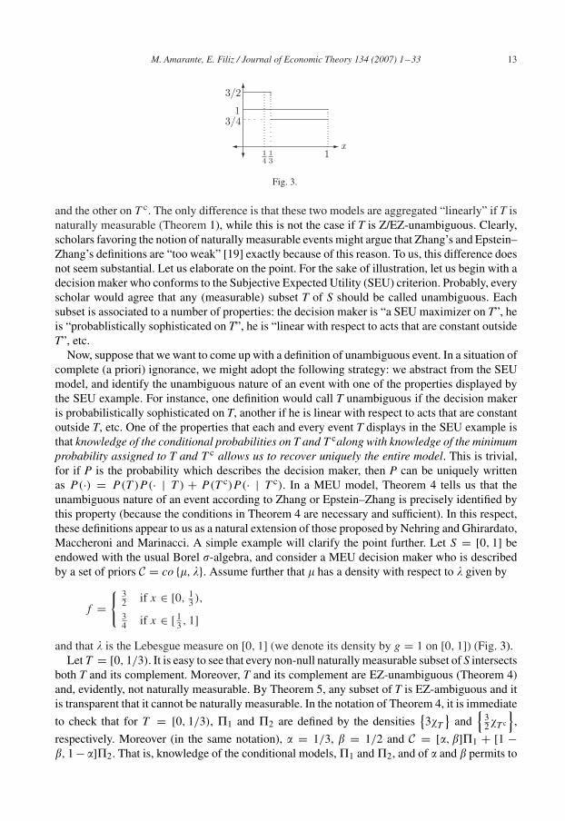
Fig. 3.

and the other on T c. The only difference is that these two models are aggregated “linearly” if T isnaturally measurable (Theorem 1), while this is not the case if T is Z/EZ-unambiguous. Clearly,scholars favoring the notion of naturally measurable events might argue that Zhang’s and Epstein–Zhang’s definitions are “too weak” [19] exactly because of this reason. To us, this difference doesnot seem substantial. Let us elaborate on the point. For the sake of illustration, let us begin with adecision maker who conforms to the Subjective Expected Utility (SEU) criterion. Probably, everyscholar would agree that any (measurable) subset T of S should be called unambiguous. Eachsubset is associated to a number of properties: the decision maker is “a SEU maximizer on T”, heis “probablistically sophisticated on T”, he is “linear with respect to acts that are constant outsideT”, etc.

Now, suppose that we want to come up with a definition of unambiguous event. In a situation ofcomplete (a priori) ignorance, we might adopt the following strategy: we abstract from the SEUmodel, and identify the unambiguous nature of an event with one of the properties displayed bythe SEU example. For instance, one definition would call T unambiguous if the decision makeris probabilistically sophisticated on T, another if he is linear with respect to acts that are constantoutside T, etc. One of the properties that each and every event T displays in the SEU example isthat knowledge of the conditional probabilities on T and T calong with knowledge of the minimumprobability assigned to T and T c allows us to recover uniquely the entire model. This is trivial,for if P is the probability which describes the decision maker, then P can be uniquely writtenas P(·) = P(T )P (· | T ) + P(T c)P (· | T c). In a MEU model, Theorem 4 tells us that theunambiguous nature of an event according to Zhang or Epstein–Zhang is precisely identified bythis property (because the conditions in Theorem 4 are necessary and sufficient). In this respect,these definitions appear to us as a natural extension of those proposed by Nehring and Ghirardato,Maccheroni and Marinacci. A simple example will clarify the point further. Let S = [0, 1] beendowed with the usual Borel �-algebra, and consider a MEU decision maker who is describedby a set of priors C = co {�, �}. Assume further that � has a density with respect to � given by

f ={ 3

2 if x ∈ [0, 13 ),

34 if x ∈ [ 1

3 , 1]and that � is the Lebesgue measure on [0, 1] (we denote its density by g = 1 on [0, 1]) (Fig. 3).

Let T = [0, 1/3). It is easy to see that every non-null naturally measurable subset of S intersectsboth T and its complement. Moreover, T and its complement are EZ-unambiguous (Theorem 4)and, evidently, not naturally measurable. By Theorem 5, any subset of T is EZ-ambiguous and itis transparent that it cannot be naturally measurable. In the notation of Theorem 4, it is immediate

to check that for T = [0, 1/3), �1 and �2 are defined by the densities{3�T

}and

{32�T c

},

respectively. Moreover (in the same notation), � = 1/3, � = 1/2 and C = [�, �]�1 + [1 −�, 1 − �]�2. That is, knowledge of the conditional models, �1 and �2, and of � and � permits to


Fig. 4.

reconstruct C uniquely. In contrast, suppose that we take A = [0, 1/4) rather than T. In this case,the conditional models are defined by the two sets of densities

{f1 = 4} and

{f2 =

{125 if x ∈ [ 1

4 , 13 );

65 if x ∈ [ 1

3 , 1]; g2 = 4

3

}.

Let �′1 and �′

2 be the corresponding sets of measures. The coefficients � and � are now 1/4 and3/8, respectively. It is immediate to see that, with these choices, C �= [�, �]�′

1 +[1−�, 1−�]�′2.

For instance, for � = 5/16, the density h = �f1 + (1 − �)f2 defines a measure ∈ [�, �]�′1 +

[1 − �, 1 − �]�′2 but /∈ C (see Fig. 4).

In other words, if A is not Z/EZ-unambiguous, knowledge of the conditional models is insuffi-cient to uncover the decision maker’s global behavior.

Transparently, the most striking difference is the lack of compatibility of Epstein–Zhang notionwith the axiom of small unambiguous event continuity. We have already commented on thisfollowing the statement Theorem 5.

We come now to our final observations. One of the main themes in the work of Zhang andEpstein–Zhang is the intuitive link between a notion of unambiguous events and Savage’s Sure-thing Principle. This intuition is transparently incorporated in their definitions. Now, supposethat, in loose terms, one interprets their view as conveying that T should be called unambiguous ifconditional on T, the decision maker is representable without reference to what happens outsideT. Consider the event A = [0, 1/4) in the example above. There is no doubt that A satisfies thecriterion. In fact, A satisfies the first part of Epstein–Zhang definition. Yet, A is ambiguous as wesaw above and the reason is that its complement fails the first part of the definition. A naturalquestion is, why should we demand that Zhang and Epstein–Zhang classes be closed undercomplementation? We do not have a clear answer. Yet, we would like to stress the legitimacy ofour question: closure under complementation is a property which follows from the definition ofnaturally measurable event, while it is imposed in the definitions of Zhang and Epstein–Zhang. Onone hand, Theorem 4 and the example of this section show that, if the classes are not closed undercomplementation, the decomposition property of Theorem 4 does not hold. Hence, if one believesthat the unambiguous nature of an event should be identified by the property we described in thefirst paragraph of this section, then there is no choice but to impose closure under complementation.On the other hand, if one’s intuition conforms to the less demanding interpretation we just gave,one should probably give up the requirement of closure under complementation.

Finally, let us observe that events like A in the example above have several special properties.In particular, A is such that all of its subsets satisfies the first part of Zhang’s definition (thedecision maker is SEU conditional on A). While events like these have been completely neglectedin the current literature, it seems indisputable to us that they deserve a place in a debate centeredaround the notion of ambiguity. Usually the idea of ambiguity is associated to that of coarse


information. In contrast, SEU or probabilistic sophistication are associated to the idea of preciseor fine information. It seems then natural to consider situations characterized by coarse informationin some parts of the state space and by fine information in some other parts. To this end, dependingon whether one leans toward SEU or probabilistic sophistication as a choice for a benchmark, oneshould identify those events with the property that each and every subevent satisfy the first partof Zhang (SEU) or Epstein–Zhang (probabilistic sophication) definition. Due to their properties,objects of this sort should be called Z-filters and EZ-filters, respectively.

To focus ideas, suppose that S = [0, 1] and let {In}n∈N be a countable partition of [0, 1], whereeach In is an interval. Using notation like that in Theorem 5, consider a MEU decision makerwith set of priors C = ∑

n∈N[�n, �n]Pn, where each Pn is a non-atomic priors supported on In,and �n �= �n. Assume further that all Pn’s are absolutely continuous with respect to the Lebesguemeasure on [0, 1]. Globally, this is a MEU decision maker with an infinite dimensional set ofpriors. However, for almost every point in [0, 1]—i.e., except for the intervals’ endpoints—thereexists a neighborhood of the point such that, conditional on that neighborhood, the decision isa SEU decision maker. Such a decision maker is associated to a countable family of Z-filters,the family of intervals {In}, none of which is either naturally measurable or Z/EZ-unambiguous.Similar examples can be given by replacing SEU with probabilistic sophistication and Z-filterswith EZ-filters.

Acknowledgments

We wish to thank Prajit Dutta, Igor Kopylov, Massimo Marinacci and Klaus Nehring for usefuldiscussions. We are grateful to a referee, whose suggestions greatly improved the paper.

Appendix A.

A.4. Naturally mesurable events

Proof of Theorem 1. Let E be an event. For f ∈ F denote by fE = f |E the restriction of fto E, and let F |E be set of all such restrictions. When E is endowed with the restriction of �to E, each element in F |E is measurable. Given E, define a preference relation �E on F |E by“fE�EgE iff f Ew�gEw for some w ∈ R”. The following lemma shows that if E is naturallymeasurable, then �E is well-defined.

Lemma 3. Let f, g ∈ F , w ∈ R and let E ∈ ANM. If f Ew�gEw for some w ∈ R, then for anyw′ ∈ R, we have f Ew′�gEw′.

Proof. If f Ew�gEw, then E naturally measurable gives

I (f Ew) � I (gEw),

minP∈C

[∫E

f (s) dP(s) + wP(Ec)

]� min

P∈C

[∫E

g(s) dP(s) + wP(Ec)

],

[minP∈C

∫E

f (s) dP(s)

]+ wP(Ec) �

[minP∈C

∫E

g(s) dP(s)

]+ wP(Ec),

16 M. Amarante, E. Filiz / Journal of Economic Theory 134 (2007) 1–33[minP∈C

∫E

f (s) dP(s)

]+ w′P(Ec) �

[minP∈C

∫E

g(s) dP(s)

]+ w′P(Ec),

I (f Ew′) � I (f Ew′),

that is f Ew′�gEw′. �

We can now prove Theorem 1. Let � = {Ti}ni=1 be a finite partition of S with the property thatTi ∈ ANM for each i and denote by F� the set of acts which are constant on each Ti . In otherwords, F� is the set of all step functions on the partition �.

Proof of Theorem 1. For any f ∈ F and any g ∈ F�, we have

I (f + g) = minP∈C

∫S

(f + g) dP

= minP∈C

[∫S

f dP +n∑

i=1

giP (Ti)

](because g ∈ F�)

=(

minP∈C

∫S

f dP

)+

n∑i=1

giP (Ti) (because each Ti ∈ ANM)

= I (f ) + I (g). �

Now, for each i, define the preference �Tiby

fTi�Ti

gTiiff f Tiw�gTiw for some w ∈ R.

By the previous lemma, �Tiis well-defined. It is easy to see that �Ti

satisfies all the axiomsof Gilboa–Schmeidler [10] (because � does). Hence, �Ti

has a MEU representation. That is,there exists a unique collection of non-empty, weak� compact, and convex set of priors CTi

, eachsupported by Ti such that ITi

: F |Ti→R defined by ITi

(f ) = minP∈CTi

∫Ti

f dP represents

�Ti. Now, define z : F →R|�| (|�| is the cardinality of �) by f �−→ (ITi

(f ))Ti∈�, and definev : R|�| → R as the unique mapping which makes the diagram below commute

F z−→ R|�|I ↘ ↓ v

R.

That is, v((ITi(f ))Ti∈�) = I (f ). To complete the proof, it suffices to show that v(.) is a positive

linear functional on R|�|.

(a) v(.) is homogeneous: Let (wi)i=1,...,n ∈ (ITi(F))Ti∈� and � ∈ R. Define an act f (s) = �wi

for s ∈ Ti . Then, v((�wi)i=1,...,n) = v((ITi(f )) = I (f ) and I (f ) = min

C

∑ni=1 �wiP (Ti) =∑n

i=1 �wiP (Ti), for any P since Ti ∈ ANM. It follows that

v((�wi)i=1,...,n) = �n∑

i=1

wiP (Ti) = � minC

n∑i=1

wiP (Ti) = �v((wi)i=1,...,n).


(b) v(.) is additive: For any (wi)i=1,...,n, (w′i )i=1,...,n ∈ (ITi

(F))Ti∈�, define a pair of acts f andg by f (s) = wi , g(s) = w′

i for s ∈ Ti . Then,

v((wi)i=1,...,n + (w′i )i=1,...,n) = v((ITi

(f ) + ITi(g))i=1,...,n)

= v((ITi(f + g))i=1,...,n)

= I (f + g)

= I (f ) + I (g) by the preceding= v((wi)i=1,...,n) + v((w′

i )i=1,...,n).

(c) v(.) is positive: Trivially because I (.) is a positive function.

Finally, since v(.) is a positive linear functional there is a positive measure q = (q1, . . . , qn)

on R|�| such that

I (f ) = v((ITi(f ))Ti∈�) =

n∑i=1

(ITi

(f ))qi =

n∑i=1

(min

P∈CTi

∫Ti

f dP

)qi

(q is a probability measure because I (1) = 1). �

A.5. Zhang and Epstein–Zhang unambiguous events

Proposition 6. Let T be such that either minC

P(T ) = 0 and maxC

P(T ) �= 0 or maxC

P(T ) = 1

and minC

P(T ) �= 1, then T is EZ-ambiguous.

Proof. Let T be such that 0 = min P(T ) < max P(T )�1. Let C1 = arg maxP∈C P(T ). SinceC1 is thin, there exists (by an easy application of Lyapunov’s convexity theorem) an event A ⊂ T

such that P(A) = 2/3P(T ) for any P ∈ C1. Consider the acts a(w) = (�A−�Ac)T w and a(w) =(�Ac − �A)T w. It is immediate to see that there exists n ∈ N such that for w� − n both actsare evaluated by P’s such that P(T ) = 0. Hence, I (a(w)) = w = I (a(w)), that is a(w)�a(w).Similarly, for w′ �n, both acts are evaluated by P’s in C1, and we have I (a(w′)) > I (a(w′)). Thesame argument with T c in the place of T completes the proof. �

A.5.1. From naturally measurable events to Zhang unambiguous events

Proof of Lemma 1. For each w, denote by Zw a measure such that minC∫

f (w) dP= ∫ f (w)

dZw. Clearly, for any w,≈I (f (w))�I (f (w)) = min

C∫

f (w) dP. Suppose that the inequality is

strict for any w, that is 6

minCMIN

∫T

f (w) dP + wPMAX(T c) >

∫T

f (w) dZw + wZw(T c),

which is equivalent to

minCMIN

∫T

f (w) dP −∫

T

f (w) dZw > w[Zw(T c) − PMAX(T c)]. (4)

6 P ∈ CMIN implies P(T c) = max. Above, this is denoted by PMAX. Of course, such a P need not be unique, but thereasoning in the proof uses its value on T c only, which is independent of the choice we make.


Then, for any w there must exist a Zw such that (i) Zw(T c) < PMAX(T c) (otherwise, we aredone); and (ii) inequality (4) is true. Consider the sequence {wn = −n} and the associated se-quence

{Zwn(T

c)}. 7 Since

{Zwn(T

c)} ⊂ [PMIN(T c), PMAX(T c)], there exists a subsequence{

Zwnk(T c)

}such that Zwnk

(T c) → x ∈ [PMIN(T c), PMAX(T c)]. We have only two possibilities:

(a) if x �= PMAX(T c), then ∃ > 0 such that x + < PMAX(T c) and ∃n such that ∀n� n

Zwnk(T c) < x + ,

which implies

Zwnk(T c) − PMAX(T c) < x + − PMAX(T c) = −� < 0.

Hence,

wnk[Zwnk

(T c) − PMAX(T c)] = −nk[Zwnk(T c) − PMAX(T c)] > nk�,

that is, the expression on the RHS of (4) is unbounded. Hence, inequality (4) must be violatedbecause the LHS is bounded. It follows that the only possibility is

(b) Zwnk(T c) → PMAX(T c).

Since f is a simple function on T, f can be written as f = ∑mi=1 �i�Ai

, {Ai}m1 a partition of T.Let P be such that

∫f (w) dP = min

CMIN

∫f (w) dP′. Then,(

minCMIN

∫T

f (w) dP

)−∫

T

f (w) dZwnk

=m∑

�iP (Ai) −m∑

�iZwnk(Ai) =

m∑�i[P(Ai) − Zwnk

(Ai)].Define

�i if sign(�i ) = sign[P(Ai) − Zwnk(Ai)]

↗�i =

↘−�i otherwise.

Then,

m∑�i[P(Ai) − Zwnk

(Ai)]�m∑

�i[P(Ai) − Zwnk(Ai)].

Let � = supi �i . Then, from inequality (4) we have that ∀n ∈ N

m

�∑

[P(Ai) − Zwnk(Ai)] > −nk[Zwnk

(T c) − PMAX(T c)]⇐⇒ �[1 − PMAX(T c) − 1 + Zwnk

(T c)] > −n[Zwnk(T c) − PMAX(T c)],

which implies � < −n, a contradiction.

7 Once again, Zwn need not be unique, but the reasoning in the proof is independent of the choice we make.


The preceding shows that there exists a w∗ such that I (f (w∗)) = ≈I (f (w∗)). That is,

minCMIN

∫T

f (w∗) dP + w∗PMAX(T c)�∫

T

f (w∗) dZ + w∗Z(T c)

for any Z /∈ CMIN. Now, we want to show that it is so for any w�w∗. 8 Let > 0, and suppose

by the way of contradiction that there exists a measure Zw∗− /∈ CMIN such that≈I (f (w∗ − )) >

I (f (w∗ − )), that is

minCMIN

∫T

f (w∗ − ) dP + (w∗ − )PMAX(T c) >

∫T

f (w∗ − ) dZw∗−

+(w∗ − )Zw∗−(Tc).

The integral on T is not affected by changes in w (by the w-invariance of≈I ). Hence, this is the

same as

minCMIN

∫T

f (w∗) dP + (w∗ − )PMAX(T c) >

∫T

f (w∗) dZw∗− + (w∗ − )Zw∗−(Tc)

which implies

minCMIN

∫T

f (w∗) dP + w∗PMAX(T c) >

∫T

f (w∗) dZw∗− + w∗Zw∗−(Tc)

+[PMAX(T c) − Zw∗−(Tc)].

But, since Zw∗− /∈ CMIN, [PMAX(T c) − Zw∗−(Tc)] > 0, and this contradicts I (f (w∗)) =

≈I (f (w∗)).

Part (b) is proven in a similar way. �

Proof of Proposition 4. We are going to show that if T ∈ AZ, then f (w)�g(w) at some wimplies

(a) ∃w∗ such that≈I (f (w∗))�

≈I (g(w∗)),

(b) ∃w∗∗ such that I (f (w∗∗))� I (g(w∗∗)).

Immediately, this implies the statement in Proposition 4 because of the w-invariance of≈I

and I .

Proof. Suppose not. Then,≈I (f (w)) <

≈I (g(w)), ∀w. Since ∀w, I (f (w))�

≈I (f (w)), we have

I (f (w)) <≈I (g(w)). Hence, for any w, I (f (w)) − I (g(w)) <

≈I (g(w)) − I (g(w)). By the

previous lemma, ∃w such that I (g(w)) = ≈I (g(w)), and at such w we would have I (f (w)) <

I (g(w)), contradicting T ∈ AZ. Similarly for part (b). �

8 This does not follow immediately. We have only shown that the strict inequality (4) has to be violated an infinitenumber of times along the subsequence we used.


A.5.2. A geometric analysis

Proof of Proposition 5. I (f (w)) = minC[∫

Tf dP + wP(T c)

].

(a) w1 �w0 implies that, for any P,∫T

f dP + w1P(T c)�∫T

f dP + w0P(T c).Hence, I (f (w1))�I (f (w0)).

(b) For any � ∈ [0, 1]

�If (w1) + (1 − �)If (w0) = � minC

[∫T

f dP + w1P(T c)

]+(1 − �) min

C

[∫T

f dP + w0P(T c)

]� min

C

[∫T

f dP + (�w1 + (1 − �)w0)P (T c)

]= If (�w1 + (1 − �)w0).

(c) Let {wn} ⊂ R be such that wn → w. Then, f (wn) → f (w) in the supnorm topology.Continuity of I implies I (f (wn)) → I (f (w)). Hence, If (wn) → If (w). �

A.5.3. Necessary and sufficient conditions

Proof of Lemma 2. We begin by establishing a simple fact. Recall that for C a set of priors, thenotation C |T stands for the set of conditional probabilities computed from probabilities in C.

Lemma 4. If CMIN |T = CMAX |T , then Condition NC in the main text is satisfied.

Proof. Let f, g be of type f (w) and g(w), with f (w)�g(w). Observe that, if CMIN |T = CMAX |T ,

then≈I (f (w))�

≈I (g(w)). This is equivalent to

minCMIN

[P(T )

∫T

f dP(· | T )+w(1−P(T )

]� min

CMIN

[P(T )

∫T

gdP(· | T )+w(1−P(T )

]which, by virtue of the assumption, is in turn equivalent to

minCMAX|T

∫T

f dP(· | T )� minCMAX|T

∫T

gdP(· | T ) ⇐⇒ I (f (w))� I (g(w)).

Hence, for any w ∈ R, If (w)� Ig(w) because of the w-invariance of the functionals≈I and I .

Now, if T ∈ AZ and f (w)�g(w) for some w, then f (w′)�g(w′) for any w′ ∈ R. By Lemma 1,

∃w∗ such that≈I (f (w∗))�

≈I (g(w∗)). Hence, the conclusion follows from the w-invariance of

≈I

and the previous observation. �

However, it is evident that, in general, the condition in the previous lemma is more than it is

necessary. A weaker condition is obtained as follows. For f of the above type, define≈�f and �f

as in section 5.3. Both sets are non-empty (because CMIN and CMAX are closed (hence, weak*-compact) in the weak*-compact set C). In general, neither set is a singleton. Note, however, that


if P and Q are in, say,≈�f , then we must have∫

T

f dP =∫

T

f dQ (5)

[from∫

f dP = ∫T

f dP + wP(T c) = ∫T

f dQ + wQ(T c) and P, Q ∈ ≈�f ].

Hence, the value minCMIN

∫T

f dP is independent of the choice of the minimizer. Similarly, forCMAX in the place of CMIN.

Lemma 2. Condition NC is equivalent to the condition that for any act f

(≈�f |T ) ∩ (�f |T ) �= ∅.

Proof of Sufficiency. The proof is essentially the same as the proof of the previous lemma. Theobservation that the value

minCMIN|T

∫T

f dP(· | T ) = 1

�minCMIN

∫T

f dP

(� = minC

P(T )) is independent of the choice of the minimizer, allows us to select any measure

in≈�f to express such a value. Hence, the proof is completed by selecting exactly those measures

in≈�f and �f whose conditionals on T coincide. �

In order to prove the necessity of the condition, we need two additional results. The first is aseparation theorem proven in [3] (In [3] , this is stated as Corollary 5). Let C1 and C2 be weak*-compact subsets of ba1(�), and assume that both C1 and C2 consist of countably additive measures.Further, assume that every measure is non-atomic and that C1 ∪ C2 is thin. All these assumptionsare satisfied in our setting. We have

Theorem 6 (Amarante and Maccheroni [3]). C1 ∩ C2 = � iff there exist A, B ∈ �, A ∩ B = ∅,such that P(A) − P(B) > 0 > Q(A) − Q(B) for any P ∈ C1 and any Q ∈ C2.

The second result is stated in the following lemma.

Lemma 5. For any f ∈ B(�), the correspondence f �−→ ≈�f (f �−→ �f ) is upper hemi-

continuous.

Proof. This is an immediate consequence of Berge’s maximum theorem (see Aliprantis andBorder [1]). �

Proof of Necessity. We are going to show that if the condition fails, then so does Condition NC.

Assume that there exists an f for which (≈�f |T ) ∩ (�f |T ) = ∅. Since f is simple, let

f =n∑i

�i�Hi+ w�T c .


Now, pick a≈Pf ∈ ≈

�f ⊂ CMIN and a Pf ∈ �f ⊂ CMAX. Then,≈Pf (· | T ) �= Pf (· | T ). Because

of the assumption, this property does not depend on the choice we made. By Theorem 6, thereexist two disjoint sets A, B ⊂ T (A, B ∈ �) such that

≈Pf (A | T ) >

≈Pf (B | T ) and Pf (A | T ) < Pf (B | T )

�⇒ ≈Pf (A) >

≈Pf (B) and Pf (A) < Pf (B) (6)

for all≈Pf ∈ CMIN and all Pf ∈ CMAX. The collection H = {Hi} is a partition of T. Consider

the partition of T given by Z = {A, B, T \(A ∪ B)}. Further consider the partition of T given byH ∧ Z . Then f is simple on H ∧ Z , and can be rewritten (in an obvious notation) as

f =m∑i

�i��i+ w�T c .

Moreover (by construction), there exist two disjoint subsets K, J ⊂ {1, . . . , m} such that∑K

��i= 1A and

∑J

��i= 1B.

Now, for > 0 consider the simple function defined by

h =∑K

(�i + )��i+∑J

(�i − )��i+

∑i /∈K∪J

�i��i+ w�T c .

Notice that for every measure Q∫h dQ −

∫f dQ = [Q(A) − Q(B)]. (7)

Claim 1. For any w ∈ R, we have

[ ≈P h(A) − ≈

P h(B)]� ≈I h(w) − ≈

If (w)�[ ≈Pf (A) − ≈

Pf (B)] (8)

and

Ih(w) − If (w)�[Pf (A) − Pf (B)]. (9)

Proof of Claim 1. From Eq. (7), we have≈I (f (w)) =

∫f (w) d

≈Pf =

∫h(w) d

≈Pf −[ ≈

Pf (A) − ≈Pf (B)]

�≈I (h(w)) − [ ≈

Pf (A) − ≈Pf (B)]

which proves one inequality in (8). As for the other,≈I (h(w)) =

∫h(w) d

≈P h =

∫f(w)d

≈P h +[ ≈

P h(A) − ≈P h(B)]

�≈I (f (w)) + [ ≈

P h(A) − ≈P h(B)].

Similarly for (9). �


Claim 2. There exist ∗ > 0 such that, for any w ∈ R,≈I h∗ (w) >

≈If (w).

Proof of Claim 2. By the way of contradiction, suppose that there is no > 0 such that≈I h(w) >

≈If (w). Then, for all > 0,

≈I h(w)�

≈If (w), and inequality (8) implies [ ≈

P h(A) − ≈P h(B)]�0

for all≈P h ∈ ≈

�h . For a sequence {n} ⊂ R++ such that n → 0, hn converges (sup-norm) to

f. Hence, the upper hemicontinuity of the correspondence f �−→ ≈�f implies that if

{≈P hn

}is a

sequence such that≈P hn

∈ ≈�hn

and≈P hn

converges to P , then P ∈ ≈�f . Clearly, such convergent

sequences exist. But, the limit measure P has the property that P (A) − P (B)�0 and cannot be

in≈�f because of (6). �We can now complete the proof of the lemma by simply observing that

≈I h∗ >

≈If , as just

shown. Moreover, by (6) and (9), If > Ih for all > 0. Hence, in particular Ih∗ < If . By

Lemma 1, ∃w∗ � min{w∗

f , w∗h∗

}such that f and h∗ are all evaluated by the

≈I functionals, that is

Iz(w∗) = ≈

I z(w∗), for z = f, h∗ . By the same reason,∃w∗∗ � max

{w∗∗

f , w∗∗h∗

}such that f andh∗

are all evaluated by the I functionals. Therefore, Ih∗ (w∗) > If (w∗) and Ih∗ (w

∗∗) < If (w∗∗).That is, if the condition in the statement fails, then there exists a pair of functions (f, h∗) suchthat Condition NC fails. �

Proof of Theorem 2. Before proving Theorem 2, we need one more lemma. By virtue of the

previous lemma, for any act f, there exist a≈Pf ∈ ≈

�f and a Pf ∈ �f whose conditionals on Tcoincide.

Lemma 6. Assume that Condition NC holds. If there exist an f and a w such that If (w) < If (w),then

either �f |T ∩ ≈�f |T = � or �f |T ∩�f |T = �.

Proof. Suppose not, that is both sets are non-empty. Hence, there exist Q1 and Q2 in �f suchthat

Q1(· | T ) = R(· | T ) for someR ∈ �f ,

Q2(· | T ) = ≈R(· | T ) for some

≈R ∈ ≈

�f . (10)

If there exist an f and a w such that If (w) < If (w), then at w we have the following inequalities∫T

f (w) dQ2 + wQ2(Tc) <

∫T

f (w) d≈R +w

≈R(T c),∫

T

f (w) dQ1 + wQ1(Tc) <

∫T

f (w) dR + wR(T c)


because both Q1 and Q2 are in �f . These are equivalent to

Q2(T )

∫T

f (w) dQ2(· | T ) − ≈R(T )

∫T

f (w) d≈R(· | T ) < w[Q2(T ) − ≈

R(T )],

Q1(T )

∫T

f (w) dQ1(· | T ) − R(T )

∫T

f (w) dR(· | T ) < w[Q1(T ) − R(T )].

By (10), these imply

[Q2(T ) − ≈R(T )]

∫T

f (w) d≈R(· | T ) < w[Q2(T ) − ≈

R(T )],

[Q1(T ) − R(T )]∫

T

f (w) dR(· | T ) < w[Q1(T ) − R(T )].

Now, let≈Pf and Pf be two measures in

≈�f and �f whose conditionals on T coincide. Such

measures exist (by Lemma 2) because we assumed that Condition NC holds. By Eq. (5) (beforethe proof of Lemma 2), we have∫

T

f (w) d≈R(· | T ) =

∫T

f (w) d≈Pf (· | T ),∫

T

f (w) dR(· | T ) =∫

T

f (w) dPf (· | T )

because both≈R and

≈Pf [R and Pf ] are in

≈�f [�f ]. Moreover,

≈Pf (· | T ) = Pf (· | T ). Hence,

the previous inequalities can be rewritten as

[Q2(T ) − ≈Pf (T )]

∫T

f (w) d≈Pf (· | T ) < w[Q2(T ) − ≈

Pf (T )],

[Q1(T ) − Pf (T )]∫

T

f (w) d≈Pf (· | T ) < w[Q1(T ) − Pf (T )]. (11)

Since neither Q1 nor Q2 are in≈�f ∪�f (because this would contradict If (w) < If (w)), we

have [Q2(T ) − ≈Pf (T )] > 0 > [Q1(T ) − Pf (T )]. Hence, inequalities (11) imply∫

T

f (w) d≈Pf (· | T ) < w and

∫T

f (w) d≈Pf (· | T ) > w

a contradiction. �

We are now ready to prove Theorem 2.

Proof of Theorem 2. Sufficiency is immediate. Necessity of (i) was shown in the first part. Wehave only to show the necessity of (ii). To this end, assume that (i) holds and suppose, by the wayof contradiction, that there exists an f (w) = f T w such that If (w) < If (w). By the previouslemma, it must be case that

either �f |T ∩ ≈�f |T = � or �f |T ∩�f |T = �.

Without loss, assume that the first set is empty. By Theorem 6 (stated in the proof of Lemma 2,

above), there exist two disjoint sets A, B ⊂ T (A, B ∈ �) such that for any≈Pf ∈ ≈

�f and any


Pf ∈ �f , we have≈Pf (A | T ) >


�⇒ ≈Pf (A) >

≈Pf (B) and Pf (A) < Pf (B). (12)

Now, we can proceed by defining a new function h, > 0, exactly as in the proof of Lemma 2.Immediately, we have that for any w′ ∈ R,

Ih(w′) − If (w′)�[Pf (A) − Pf (B)]. (13)

The proof of this statement is exactly the same as the proof of Claim 1 in the proof of Lemma

2. For any > 0, there exists (by Lemma 1) a w∗ such that, If (w∗

) = ≈If (w∗

) and Ih(w∗ ) =

≈I h(w

∗ ). By Claim 2 in the proof of Lemma 2, we can find an ∗ (and an associated w∗

) such thatIh∗ (w

∗ ) > If (w∗

). At w, by assumption If (w) < If (w). It then follows from (12) and (13),that If (w) > Ih(w) for all > 0. That is, the expression [If (w′) − Ih(w

′)] changes sign as wvaries, and this contradicts T ∈ AZ. �

A.5.4. Epstein–Zhang unambiguous events

Let f be such that (≈�f |T ) ∩ (�f |T ) = ∅. From Theorem 6, we know that there exist two

disjoint sets A, B ⊂ T (A, B ∈ �) such that≈Pf (A | T ) >


�⇒ ≈Pf (A) >

≈Pf (B) and Pf (A) < Pf (B)

for all≈Pf ∈ CMIN and a Pf ∈ CMAX. Define r = �A − �B and r = �B − �A, and, for > 0,

consider the two functions

h(w) = f (w) + r(0) and g(w) = f (w) + r(0).

Lemma 7. If there exists an f for which (≈�f |T ) ∩ (�f |T ) = ∅, then, there exist > 0 and two

points, w and w′ such that

I (h(w)) > I (f (w)) > I (g(w)) and I (h(w′)) < I (f (w′)) < I (g(w

′)).

Proof. The existence of an ∗ > 0 and of two points w and w′ such that I (h∗(w)) > I (f (w))

and I (h∗(w′)) < I (f (w′)) was already shown in Lemma 2. Moreover, the last inequality holdsfor any > 0 (see proof of Lemma 2). By a similar argument, one shows that there exists an∗∗ > 0 such that (see proof of Lemma 2)

I (h∗(w)) > I (f (w)) > I (g∗∗(w)) and I (h∗(w′)) < I (f (w′)) < I (g∗∗(w′))

with the inequality I (f (w)) > I (g(w)) holding for any > 0. To complete the proof, we onlyneed to show that we can choose the same for both h and g. To this end, it suffices to show that

I (h∗(w)) > I (f (w)) �⇒ I (h(w)) > I (f (w)) for any 0 < < ∗,I (g∗∗(w′)) > I (f (w′)) �⇒ I (g(w

′)) > I (f (w′)) for any 0 < < ∗∗.This follows straight from the concavity of I . In fact, noticing that for any 0 < < ∗,

h(w) = �h∗(w) + (1 − �)f (w) some � ∈ (0, 1),


we have

I (h(w))��I (h∗(w)) + (1 − �)I (f (w)) > I (f (w))

and similarly for I (g(w′)). �

Proof of Theorem 3. The inclusion AZ ⊂ AEZ comes straight out of the definitions. We aregoing to show that T /∈ AZ �⇒ T /∈ AEZ thus showing that AZ ⊃ AEZ. First, suppose thatcondition (i) in Theorem 2 is violated. Then, there exist g and h like in the previous lemma sothat (recall that, from Lemma 1, the points w and w′ can be chosen so that I in the inequalities inLemma 7 can be taken equal to I)

I (h(w)) > I (f (w)) > I (g(w)) and I (h(w′)) < I (f (w′)) < I (g(w

′)).

Now, for n�1, consider the functions{

1nf (w)

}n�1

. It is easy to check that there exist a w¯

and an n¯

such that arg minC

∫ 1nf (w

¯) dP ∈ CMIN for all n�n

¯(because eventually 1

nf is in a

neighborhood of the function that is identically 0 on T). Similarly, there exist w and n such thatarg min

C

∫ 1nf (w) dP ∈ CMAX for all n� n. Next, observe that

≈�f (w) = arg min

P∈CMIN

(∫f (w) dP

)= ≈

� 1nf (w)

= arg minP∈CMIN

(∫1

nf (w) dP

),

�f (w) = arg minP∈CMAX

(∫f (w) dP

)= � 1

nf (w)

= arg minP∈CMAX

(∫1

nf (w) dP

). (14)

Define

g,n(w) = 1

nf (0) + r(w), h,n(w) = 1

nf (0) + r(w).

For n� max {n, n¯}, it follows from the previous lemma and the equalities (14) that

I (h,n(w)) > I

(1

nf (w)

)> I (g,n(w)) ∀w�w

¯, (15a)

I (h,n(w′)) < I

(1

nf (w′)

)< I (g,n(w

′)) ∀w′ �w. (16)

Notice that for w�w¯

, I in (15a) is equal to≈I . Similarly, for w′ �w, I in (16) is equal to I (see

proof of Lemma 2). Taking the limits for n → ∞ of both (15a) and (16) and using the (sup-norm)continuity of I, we have

I (r(w))�w≈P(T c)�I (r(w)) ∀w�w

¯, (17a)

I (r(w))�wP (T c)�I (r(w)) ∀w′ �w. (18)

Now, we claim that at least one inequality in (17a) is strict. In fact, at w�w¯

I (r(w)) = minCMIN

{∫

[(�B − �A) + w�T c ] dP

}= min

CMIN

∫

(�B − �A) dP + w≈P(T c) < w

≈P(T c)


because, for any n,≈� 1

nf (w)

⊂ CMIN, and we know that≈� 1

nf (w)

contains at least a measure P

(in fact, all) such that P(B) − P(A) < 0. Since r(w) and r(w) are EZ-conjugate, this showsthat T is EZ-ambiguous.

Finally, a proof that T is EZ-ambiguous if condition (i) in Theorem 2 is satisfied but condition(ii) is violated is obtained exactly along the same lines by taking into account Lemma 6 (see proofof Theorem 2). �

A.6. Applications

Proof of Theorem 4. We prove the statement only for acts of the form f T w. The proof for actsof the form f T cw follows at once by exchanging T and T c.

(Necessity) Fix an MEU model with set of priors C. Since T ∈ AZ, we have I = I for all acts

of type f T w (Theorem 2). Hence, I (f (w)) = min

{≈I (f (w)), I (f (w))

}.≈I (f (w)) and I (f (w))

can be written as

I (f (w)) = � minCMAX|T

∫T

f dP(· | T ) + w(1 − �),

≈I (f (w)) = � min

CMIN|T

∫T

f dP(· | T ) + w(1 − �).

Let �1 = co {CMAX |T ∪CMIN |T }, �2 = co {CMAX |T c ∪CMIN |T c} and define C∗ = [�, �]�1 ×[1 − �, 1 − �]�2. For any f (w), it can be readily checked that

minC∗

∫f (w) dP

= min

{� min

�1

∫T

f dP(· | T ) + w(1 − �), � min�1

∫T

f dP(· | T ) + w(1 − �)

}.

Since �1 ⊃ CMAX |T ∪CMIN |T , we have

minC∗

∫f (w) dP� min

C

∫f (w) dP. (19)

We are going to show that equality holds. By definition of �1, any minimizer of∫T

f dP(· | T )

is either in CMAX |T or in CMIN |T . Hence, let P ∈ CMAX |T ∪CMIN |T be such that∫T

f dP =min

C∫

f dP. Suppose that P ∈ CMAX |T . By definition, there exists a_P ∈ CMAX whose conditional

on T coincides with P .

Claim. If Q ∈ �f , then∫T

f dQ(· | T )�∫T

f dP .

In fact, Q ∈ �f implies that for any measure in CMAX, hence for_P , we have

minCMAX

∫f dP =

∫f dQ = Q(T )

∫T

f dQ(· | T ) + wQ(T c)

�_P (T )

∫T

f dP (· | T ) + w

_P (T c)

which implies∫T

f dQ(· | T )�∫T

f dP . By definition, Q(· | T ) ∈ CMAX |T (because �f ⊂CMAX). Hence,

∫T

f dQ(· | T ) = ∫T

f dP . Since T ∈ AZ, Condition NC holds and by Lemma 2


(≈�f |T ) ∩ (�f |T ) �= ∅. That is, there exists a

≈Pf (· | T ) ∈ (

≈�f |T ) such that

∫T

f dP =∫T

f d≈Pf (· | T ). By definition,

≈Pf (· | T ) ∈ CMIN |T . Summing up, for any f (w)

min�1

∫T

f (w) dP = minCMAX|T ∪CMIN|T

∫T

f (w) dP =∫

T

f dP (20)

=∫

T

f dQ(· | T ) = minCMAX|T

∫T

f (w) dP = minCMIN|T

∫T

f (w) dP.

Similarly, we reach the same conclusion if we start by assuming that P ∈ CMIN |T .Now, (20) show that equality holds in (19), that is

minC∗

∫f dP = I = min

C

∫f dP.

(Sufficiency) Immediate.The equality AZ = AEZ was shown in Theorem 3. Finally, if T ∈ ANM, T c ∈ ANM, Theorem

1 applies and C = C∗ = ��1 + [1 − �]�2. In the converse direction, suppose that T ∈ AEZ andthat � = �. Suppose, by contradiction that T /∈ ANM, then there must exist a P ∈ C\C∗ such thatP(T ) �= �. It is easy to see that, in such a case, there is an act of the form xTy, x, y ∈ R, suchthat min

C∫

xTy dP �= minC∗∫

xTy dP which contradicts the first part of the theorem. �

Proof of Theorem 5. We divide the proof into several claims. To begin, let T ∈ AZ\ANM andlet A ⊂ T . Define

CTMAX = arg max

P∈CP(T ), CA

MAX = arg maxP∈C

P(A)

and define CTMIN and CA

MIN similarly. Let � = min P(T ), � = max P(T ), � = min P(A), and� = max P(A). Assume � �= � and � �= �.

Claim 1. CTMAX ∩ CA

MAX �= �, and CTMIN ∩ CA

MIN �= �.

Proof. Let f (w) = 0Aw. Observe that f (w) is an act which is constant both on Ac and onT c. Therefore, by Theorems 4 and 2, I (f (w)) = I T (f (w)) = I A(f (w)), where I ·(f (w)) =min{ min

P∈C·MIN

∫f (w) dP, min

P∈C·MAX

∫f (w) dP}. We have,

I T (f (w))= min

{�( min

P∈CTMIN

(wP (T \A|T )−w))+w, �( minP∈CT

MAX

(wP (T \A|T )−w))+w

}.

By (≈�f |T ) ∩ (�f |T ) �= ∅ (Lemma 2), min

P∈CTMIN

(wP (T \A|T ) − w)) = minP∈CT

MAX

(wP (T \A|T ) − w)). Since w > 0, we have

I T (f (w) = �( minP∈CT

MAX

(wP (T \A|T ) − w)) + w

= �(wP ∗(T \A|T ) − w)) + w for some P ∗ ∈ CTMAX

= I A(f (w)) = min�,�

{w(1 − �), w(1 − �)} = w(1 − �).


Hence, �(wP ∗(T \A|T ) − w)) + w = w(1 − �) which implies

P ∗(T \A|T ) = � − �

�.

From which we conclude (since P ∗ ∈ CTMAX) that

P ∗(T \A) = � − � �⇒ P ∗(A) = � �⇒ P ∗ ∈ CAMAX �⇒ CA

MAX ∩ CTMAX �= �.

Similarly, one shows that CTMIN ∩ CA

MIN �= � by taking w < 0. �

Before tackling the proof of Theorem 5, we need one more observation. Let f ∈ F be a threestep act f = [k, A; k′, T \A; k

′′, T c] (this notation was explained in Section 3). Such an act can

be thought of in two different ways. As an act of the form f T k′′

and as an act of the form f Ack.

For T ∈ AEZ, from Theorem 2 we have that I (f (k′′)) = I T (f (k′′)). Hence,

I T (f (k′′))

= min

{�

(min

P∈CTMIN

(k − k′)P (A|T ) + k′ − k′′)

+k′′, �

(min

P∈CTMAX

(k − k′)P (A|T ) + k′ − k′′)

+ k′′}

.

By choosing k′′

small enough, we can guarantee that � and some P ∈ CTMIN attain the minimum.

Moreover, for k > k′ we can guarantee that the P in CTMIN is such that P(A) = � (existence of

such a P in CTMIN was shown in Claim 1 above).

In the same fashion, by choosing k′′

big enough, we can guarantee that the minimum obtainsfor � and some P ′ in CT

MAX. Moreover, for k > k′ such a P ′ would be such that P ′(A) = � =minP∈CT

MAXP(A) is used. Summarizing, for k > k′ the evaluation of a three step act like ours is

either

I T (f (k′′)) = �k + (� − �)k′ + (1 − �)k

′′(21)

or

I T (f (k′′)) = �k + (� − �)k′ + (1 − �)k

′′. (22)

By definition of �, and �, we have ��.We can prove our first result. The proof is restricted to the case � < �. The case � = � will be

dealt with in the proof of Proposition 8, below.

Proposition 7. If T ∈ AEZ\ANM, then there is no A ⊂ T such that A ∈ AEZ\ANM.

Proof. We proceed by contradiction. Let f (k′′)=[k, A; k′, T \A; k

′′, T c], g(k

′′)=[t, A; t ′, T \A;

k′′, T c], f (k) = [k, A; k′, T \A; k, T c] and g(k) = [t, A; t ′, T \A; k, T c], where we choose

k > k′ and t > t ′. For k′′

small enough we can guarantee that f (k′′) and g(k

′′) are evaluated as


(b)(a)

Fig. 5.

in (21), i.e.

I (f (k′′)) = I T (f (k

′′)) = �k + (� − �)k′ + (1 − �)k′′,

I (g(k′′)) = I T (g(k

′′)) = �t + (� − �)t ′ + (1 − �)k′′

while for k big enough we can guarantee that f (k) and g(k) are evaluated as in (22), i.e.

I (f (k)) = I T (f (k)) = �k + (� − �)k′ + (1 − �)k,

I (g(k)) = I T (g(k)) = �t + (� − �)t ′ + (1 − �)k.

Let us rename variables by setting

x = k − t; y = k′ − t ′; a = �; b = � − �; c = �; d = � − �. (23)

Case 1: ab

< cd

. We have

I (f (k′′)) − I (g(k

′′)) = ax + by and I (f (k)) − I (g(k)) = cx + dy.

By choosing x and y as in Fig. 5(a), we get I (f (k′′))− I (g(k

′′)) > 0 and I (f (k))− I (g(k)) < 0,

thus contradicting T ∈ AEZ.Case 2: a

b> c

d. By choosing x and y as in Fig. 5(b), we get I (f (k

′′)) − I (g(k

′′)) > 0 and

I (f (k)) − I (g(k)) < 0, again contradicting T ∈ AEZ.Case 3: a

b= c

d. We distinguish between two subcases.

Case 3.1: b > d. Observe that

b > d ⇐⇒ � − � > � − � ⇐⇒ 2�

� − �<

2�

� − ��⇒ 2�

� − �<

� + �

� − �.

Now, take an > 0 and choose � so that 0 <

(2�

� − �

) < � <

(� + �

� − �

). Next, choose k > 0

big enough so that − (� − �)

b − dk + � < −. Define

k = ; t = −; k′ = − (� − �)

b − dk; t ′ = k′ + �. (24)

By choosing k′′

small enough so that both f (k′′) and g(k′′) are evaluated as in (21), we have

I (f (k′′)) − I (g(k

′′)) = �(k − t) + (� − �)(k′ − t ′) = �2 + (� − �)(−�) < 0. (25)


On the other hand, by definition of a and c, we have a < c. Hence,

(a − c) < 0

⇐⇒(a − c)k + (b − d)k′ + (� − �)k < 0 (by (24))

⇐⇒�k + (� − �)k′ + (1 − �)k < �k + (� − �)k′ + (1 − �)k (by (23)).

That is, I (f (k)) = �k + (� − �)k′ + (1 − �)k. Next, observe that c > a, b > d and � > 0 imply

(c − a)(−) + (d − b)� < 0

⇐⇒(c−a)t+(d−b)t ′+(�−�)k < 0 (because (d−b)t ′+(�−�)k=(d−b)� by (24))

⇐⇒�t + (� − �)t ′ + (1 − �)k < �t + (� − �)t ′ + (1 − �)k (by (23)).

That is, I (g(k)) = �t + (� − �)t ′ + (1 − �)k. Summing up,

I (f (k)) − I (g(k)) = (� + �) − (� − �)� > 0. (26)

Now, inequality (25) and inequality (26) contradict the assumption T ∈ AEZ.Case 3.2: b < d

Here, we consider acts which are constant on A, and we will produce a contradiction withthe hypothesis that A ∈ AEZ (⇐⇒ Ac ∈ AEZ). Let f (k) = [k, A; k′, T \A; k

′′, T c], g(k) =

[k, A; t ′, T \A; t′′, T c], with k > k′ and k > t ′, and let f (k) = [k, A; k′, T \A; k

′′, T c], g(k) =

[k, A; t ′, T \A; t′′, T c] with k > k′ and k > t ′. Set

k = −; t ′ = −2; k′ = t ′ −

� − �; t

′′ = ; k′′ = t ′′ +

1 − �.

Choose k big enough so that both f (k) and g(k) are evaluated as in (21), we have

I (f (k)) − I (g(k)) = (� − �)(k′ − t ′) + (1 − �)(k′′ − t

′′)

= (� − �)

(−

� − �

)+ (1 − �)

(

1 − �

).

That is,

I (f (k)) − I (g(k)) = 0. (27)

Next, observe that c > a, d > b, � > � (see (23); d > b by the assumption) imply

(c − a)(−) + (d − b)

(−2 −

� − �

)+ (� − �)( +

1 − �) < 0

⇐⇒(c − a)k + (d − b)k′ + (� − �)k

′′< 0.

That is

�k + (� − �)k′ + (1 − �)k′′

< �k + (� − �)k′ + (1 − �)k′′

(see(23))


which implies I (f (k)) = �k + (� − �)k′ + (1 − �)k′′. On the other hand, c > a, d > b and

� > � also imply

(c − a)(−) + (d − b)(−2) + (� − �) < 0

⇐⇒(c − a)k + (d − b)t ′ + (� − �)t

′′< 0

⇐⇒�k + (� − �)t ′ + (1 − �)t

′′< �k + (� − �)t ′ + (1 − �)t

′′(see(23)).

That is, I (g(k)) = �k + (� − �)t ′ + (1 − �)t′′. Combining the last two findings,

I (f (k)) − I (g(k)) = −

(� − �)(1 − �)[d − b] < 0. (28)

Now, equality (27) and inequality (28) contradict Ac ∈ AEZ. To complete the proof, the only caseleft to consider is � = �. This can be dealt with by using the same construction as in the proof ofProposition 8, below. �

Proposition 8. If T ∈ AEZ\ANM, then there is no A ⊂ T such that A ∈ ANM.

Proof. By the way of contradiction, assume that such an A exists. Recall that A ∈ ANM means� = � = �. For any three step act f (k

′′) = [k, A; k′, T \A; k

′′, T c], we have

I (f (k′′)) = I T (f (k

′′))

= min{�k + (� − �)k′ + (1 − �)k

′′, �k + (� − �)k′ + (1 − �)k

′′}.

Hence,

k′ > k′′ �⇒ I (f (k′′)) = �k + (� − �)k′ + (1 − �)k

′′, (29)

k′ < k′′ �⇒ I (f (k′′)) = �k + (� − �)k′ + (1 − �)k

′′. (30)

Now, let f (k′′) = [k, A; k′, T \A; k′′, T c], g(k

′′) = [t, A; t ′, T \A; k

′′, T c] for some k′ > k

′′and

t ′ > k′′, and let f (k) = [k, A; k′, T \A; k, T c], g(k) = [t, A; t ′, T \A; k, T c] for some k > k′

and t ′ > k. Notice that all these acts are constant on T c. Let > 0, and define

k′ = 0; k = ; t ′ = 2; t = 0; k = (� − �)2

�+ �

�,

where � is chosen so that 0 < � < (� − �). For k′′

small enough, both f (k′′) and g(k

′′) are

evaluated as in (29). Thus,

I (f (k′′)) − I (g(k

′′)) = � > 0. (31)

Next, observe that by construction t ′ > k > k′, which implies that f (k) is evaluated as in (30)while g(k) is evaluated as in (29). Thus, by our choice of �

I (f (k)) − I (g(k)) = � + (� − �) < 0. (32)

Now, inequality (31) and inequality (32) contradict T ∈ AEZ. �

This, along with Proposition 7 completes the proof of Theorem 5.


Proof of Corollary 1. It is immediate that � and S are in AEZ. Moreover, by definition, AEZ isclosed under complementation. Now, we need to show that if A, B are in AEZ and A ∩ B = �,then A ∪ B ∈ AEZ. We are going to show that if A, B are in AEZ and A ∩ B = �, A �= Bc, thenboth A and B are necessarily naturally measurable. Then, the property follows from the fact thatnaturally measurable events make up a �-system.

To begin, suppose that B ∈ AEZ\ANM. Then, Bc ∈ AEZ because AEZ is closed under com-plementation, and Bc /∈ ANM (because otherwise one would contradict B ∈ AEZ\ANM). Thatis, Bc ∈ AEZ\ANM. By assumption, A ∩ B = � which implies Bc ⊃ A (strictly). By Theorem5, this contradicts A ∈ AEZ. That is, B ∈ ANM. By reversing the role of A and B, one showsA ∈ ANM.

Finally, the property that AEZ is closed under countable disjoint unions follows from the factthat ANM is. �

References

[1] C. Aliprantis, K. Border, Infinite Dimensional Analysis, Springer, Berlin, 1994.[2] M. Amarante, Ambiguity, Measurability and Multiple Priors, Econ. Theory 26 (2005) 995–1006.[3] M. Amarante, F. Maccheroni, When an event makes a difference, Theory and Decisions, 2006, forthcoming.[4] A. Chateauneuf, F. Maccheroni, M. Marinacci, J.-M. Tallon, Monotone continuous multiple priors, Econ. Theory 26

(2005) 973–982.[5] L.E. Dubins, D. Margolies, Naturally integrable functions, Pacific J. Math. 87 (1980) 299–312.[6] D. Ellsberg, Risk, ambiguity and the savage axioms, Quart. J. Econ. 75 (1961) 643–669.[7] L.G. Epstein, J. Zhang, Subjective probabilities on subjectively unambiguous events, Econometrica 69 (2001)

265–306.[8] P. Ghirardato, F. Maccheroni, M. Marinacci, Differentiating ambiguity and ambiguity attitude, J. Econ. Theory 118

(2004) 133–173.[9] P. Ghirardato, M. Marinacci, Risk, ambiguity and the separation of utility and beliefs, Math. Oper. Res. 26 (2001)

864–890.[10] I. Gilboa, D. Schmeidler, Maxmin expected utility with a non-unique prior, J. Math. Econ. 18 (1989) 141–153.[11] M.I. Kadec, A. Pelczynski, Bases, lacunary sequences and complemented subspaces inLp , Studia Math XXI (1962)

161–176.[12] J.F.C. Kingman, A.P. Robertson, On a theorem of Lyapunov, J. London Math. Soc. 43 (1968) 347–351.[13] P. Klibanoff, M. Marinacci, S. Mukerji, A smooth model of decision making under ambiguity, Econometrica, 2006,

forthcoming.[14] I. Kopylov, Procedural rationality in the multiple priors model, University of Rochester, Mimeo, 2002.[15] I. Kopylov, Subjective probabilities on “Small” Domains, University of Rochester, Mimeo, 2003.[16] F. Maccheroni, M. Marinacci, A. Rustichini, Variational representation of preferences under ambiguity, ICER WP

5/04, 2004.[17] K. Nehring, Capacities and probabilistic beliefs: a precarious coexistence, Math. Soc. Sci. 38 (1999) 197–213.[18] K. Nehring, Ambiguity in the context of probabilistic beliefs, UC Davis, Mimeo, 2001.[19] K. Nehring, Is it possible to define subjective probabilities in behavioral terms? A comment on Epstein–Zhang, UC

Davis, Mimeo, 2004.[20] L.J. Savage, The Foundations of Statistics, Dover, New York, 1972.[21] D. Schmeidler, Subjective probability and expected utility without additivity, Econometrica 57 (1989) 571–587.[22] J. Zhang, Subjective ambiguity, expected utility and Choquet expected utility, Econ. Theory 20 (2002) 159–181.

ambiguous events and maxmin expected...

Documents