Purely Subjective Maxmin Expected Utility∗

Shiri Alon†‡and David Schmeidler§

March 4, 2014

Abstract

The Maxmin Expected Utility decision rule suggests that the decision maker

can be characterized by a utility function and a set of prior probabilities,

such that the chosen act maximizes the minimal expected utility, where the

minimum is taken over the priors in the set. Gilboa and Schmeidler axiomatized

the maxmin decision rule in an environment where acts map states of nature

into simple lotteries over a set of consequences. This approach presumes that

objective probabilities exist, and, furthermore, that the decision maker is an

expected utility maximizer when faced with risky choices (involving only objective

probabilities). This paper presents axioms for a derivation of the maxmin

decision rule in a purely subjective setting, where acts map states to points in

a connected topological space. This derivation does not rely on a pre-existing

notion of probabilities, and, importantly, does not assume the von Neuman &

Morgenstern (vNM) expected utility model for decision under risk. The axioms

employed are simple and each refers to a bounded number of variables.

Keywords: Maxmin Expected Utility, Purely subjective probability, Uncertainty

aversion, Tradeoff consistency, Biseparable preference

JEL classification: D81

∗This is an extended and revised version of the paper presented under the same title at RUD

2008 in Oxford UK.†Corresponding author.‡Bar-Ilan University, Ramat Gan, Israel, email: shiri.aloneron@gmail.com§Interdisciplinary Center Herzliya, Tel Aviv University, and Ohio State University, email:

davidschmeidler@gmail.com

We thank the Israeli Science Foundation for a partial financial support.

Contents

1 Introduction 1

2 Tradeoffs approach 6

2.1 Basic axioms and tradeoff consistency . . . . . . . . . . . . . . . . . . . . . . . . . . 7

2.2 New axioms and the main result . . . . . . . . . . . . . . . . . . . . . . . . . . . . . 10

3 Biseparable approach 14

3.1 Basic axioms and act independence . . . . . . . . . . . . . . . . . . . . . . . . . . . . 14

3.2 New axioms and the main result . . . . . . . . . . . . . . . . . . . . . . . . . . . . . 16

4 Extensions and Comments 18

4.1 Bounded acts . . . . . . . . . . . . . . . . . . . . . . . . . . . . . . . . . . . . . . . . 18

4.2 Preference relations admitting CEU and MEU representations . . . . . . . . . . . . 18

4.3 A generalization of Theorem 1 . . . . . . . . . . . . . . . . . . . . . . . . . . . . . . 20

4.4 Purely subjective Variational Preferences . . . . . . . . . . . . . . . . . . . . . . . . 21

5 Appendix: The proofs 22

5.1 Proof of Theorem 1: (1)⇒(2) . . . . . . . . . . . . . . . . . . . . . . . . . . . . . . . 22

5.1.1 Proof of Proposition 7 . . . . . . . . . . . . . . . . . . . . . . . . . . . . . . . 22

5.2 Proof of the implication (1)⇒(2) of Theorem 1 - continued . . . . . . . . . . . . . . 26

5.3 Proof of the implication (2)⇒(1) of Theorem 1 . . . . . . . . . . . . . . . . . . . . . 35

5.4 Proof of Theorem 2 . . . . . . . . . . . . . . . . . . . . . . . . . . . . . . . . . . . . . 36

5.5 Proof of Theorem 4 . . . . . . . . . . . . . . . . . . . . . . . . . . . . . . . . . . . . 37

5.5.1 Proof of the implication (1)⇒(2) of Theorem 4. . . . . . . . . . . . . 38

5.5.2 Proof of the implication (2)⇒(1) of Theorem 4. . . . . . . . . . . . . 40

5.6 On the equivalence of tradeoff consistency definitions . . . . . . . . . . . . . . . . . 41

1 Introduction

There is a respectable body of literature dealing with axiomatic foundations of decision

theory, and specifically with the non-Bayesian (or extended Bayesian) branch of it.

We will mention a part of this literature to put our paper in context.

Building on the works of Ramsey (1931), de Finetti (1937), and von Neumann and

Morgenstern (1944, 1953), Savage (1952, 1954) provided an axiomatic model of purely

subjective expected utility maximization. The descriptive validity of this model was

put in doubt long ago. Today many think that Savage’s postulates do not constitute

a sufficient condition for rationality, and some doubt that they are all necessary

conditions for it. However, almost all agree that his work is by far the most beautiful

and important axiomatization ever written in the social or behavioral sciences. ”The

crowning glory”, as Kreps (1998, p. 120) put it. Savage’s work has had a tremendous

influence on economic modeling, convincing many theorists that the only rational

way to make decisions is to maximize expected utility with respect to a subjective

probability. Importantly, due to Savage’s axioms, many believe that any uncertainty

can and should be reduced to risk, and that this is the only reasonable model of

decision making on which economic applications should be based. About a decade

after Savage’s seminal work Anscombe and Aumann (1963) (AA for short) suggested

another axiomatic derivation of subjective probability, coupled with expected utility

maximization. As in Savage’s model, acts in AA’s model map states of nature to a set

of consequences. However, in Savage’s model the set of consequences has no structure,

and it may consist of merely two elements, whereas AA assume that the consequences

are lotteries as in vNM’s model, namely, distributions over a set of outcomes, whose

support is finite. Moreover, AA impose the axioms of vNM-’s- theory (including the

independence axiom) on preferences over acts, which imply that the decision maker

maximizes expected utility in the domain of risk. On the other hand, AA’s model can

deal with a finite state space, whereas Savage’s axioms imply that there are infinitely

many states, and, moreover, that none of them is an “atom”. Since in many economic

applications there are only finitely many states, one cannot invoke Savage’s theorem

to justify the expected utility hypothesis in such models.

A viable alternative to the approaches of Savage and of AA is the assumption that

the set of consequences is a connected topological space. (See Fishburn (1970) and

Kranz, Luce, Suppes, and Tversky (1971) and the references therein.) These spaces

1

are ”rich” and therefore more restrictive than Savage’s abstract set of consequences.

On the other hand, such spaces are natural in many applications. In particular,

considering a consumer problem under uncertainty the consequences are commodity

bundles which, in the tradition of neoclassical consumer theory, constitute a convex

subset of an n-dimensional Euclidean space, and thus a connected topological space.

As opposed to AA’s model, the richness of the space is not necessarily derived from

mixture operations on a space of lotteries. Thus, no notion of probability is pre-

supposed, and no restrictions are imposed on the decision maker’s behavior under

risk.

Despite the appeal of Savage’s axioms, the Bayesian approach has come under

attack on descriptive and normative grounds alike. In accord with the view held

by Keynes (1921), Knight (1921), and others, Ellsberg (1961) showed that Savage’s

axioms are not necessarily a good description of how people behave, because people

tend to prefer known to unknown probabilities. Moreover, some researchers argue

that such preferences are not irrational. This was also the view of Schmeidler (1989),

who suggested the first axiomatically based, general-purpose model of decision making

under uncertainty, allowing for a non-Bayesian approach and a not necessarily neutral

attitude to uncertainty. Schmeidler axiomatized expected utility maximization with

a non-additive probability measure (also known as capacity), where the operation of

integration is done as suggested by Choquet (1953-4). Schmeidler (1989) employed the

AA model, thereby using objective probabilities and restricting attention to expected

utility maximization under risk. Following his work, Gilboa (1987) and Wakker (1989)

axiomatized Choquet Expected Utility theory (CEU) in purely subjective models; the

former used Savage’s framework, whereas the latter employed connected topological

spaces. Thus, when applying CEU, one can have a rather clear idea of what the

model implies even if the state space is finite, as long as the consequence space is rich

(or vice versa).

Gilboa and Schmeidler (1989) (GS hereafter) suggested the theory of Maxmin

Expected Utility (MEU), according to which beliefs are given by a set of probabilities,

and decisions are aimed to maximize the minimal expected utility of the act chosen

(see also Chateauneuf (1991)). This model has an overlap with CEU: when the

non-additive probability is convex, CEU can be described as MEU with the set of

probabilities being the core of the non-additive probability. More generally, CEU can

capture modes of behavior that are incompatible with MEU, including uncertainty-

2

liking behavior. On the other hand, there are many MEU models that are not CEU.

Indeed, even with finitely many states, where the dimension of the non-additive

measures is finite, the dimension of closed and convex sets of measures is infinite

(if there are at least three states).1 Moreover, there are many applications in which

a set of priors can be easily specified even if the state space is not explicitly given.

As a result, there is an interest in MEU models that are not necessarily CEU. GS

axiomatized MEU in AA’s framework, paralleling Schmeidler’s original derivation of

CEU.

There are several reasons to axiomatize the MEU model without using objective

probabilities. The raison d’etre of the CEU and MEU models (and of several more

recent models) is the assumption that, contrary to Savage’s claim, Knightian uncertainty

cannot be reduced to risk. Thus to require the existence of exogenously given additive

probabilities while modeling Knightian uncertainty appear to be in a conceptual

dissonance. Another drawback of the AA framework is the assumption that it is

immaterial whether objective or subjective uncertainty is resolved first. While this

assumption is natural under subjective expected utility, it is questionable under non-

expected utility models. In addition, alternatives in the AA framework are two-stage

acts which are remote from individuals’ experience and economic models.

Most of the applications in economics assume consequences lie in a convex subset

of, say, a Euclidean space, but do not assume linearity of the utility function. It

is therefore desirable to have an axiomatic derivation of the MEU decision rule in

this framework that is applicable to a finite state space and that does not rely on

objective probabilities. Such a derivation can help us see more clearly what the exact

implication of the rule is in many applications, without restricting the model in terms

of decision making under risk or basing it on vNM utility theory.

Our goal here is to suggest a set of axioms delivering MEU representation, namely

the existence of a utility function u on the set of consequences X, and a non empty,

compact and convex set C of finitely additive probability measures on (S,Σ) (the

1The space of all convex compact subsets of the plane with the Hausdorff metric can be embedded

as a non negative cone of a linear topological space of infinite dimension. In this cone the set of all

convex closed subsets of some non degenerate triangle includes an open set of the linear topological

space. Such a triangle can represent all probability distributions over some state space with three

states.

3

states set, the events set), such that for any two acts f and g:

f % g ⇔ minP∈C

∫S

u(f(·))dP ≥ minP∈C

∫S

u(g(·))dP .

The first axiomatic derivation of MEU of this type is by Casadesus-Masanell,

Klibanoff and Ozdenoren (2000). Another one is by Ghirardato, Maccheroni, Marinacci

and Siniscalchi (2003). These are discussed in subsections 2.2 and 3.2, correspondingly.

To compare these works with ours, we continue the introduction with a comment on

axiomatization of the individual decision making under (Knightian) uncertainty. Such

an axiomatization consists of a set of restrictions on preferences. This set usually

constitutes a necessary and sufficient condition for the numerical representation of

the preferences.

Axiomatizations may have different goals and uses, be distinguished across more

than one normative or positive interpretations and be evaluated according to different

tests. Here we emphasize and delineate simplicity and transparency as a necessary

condition for an axiom. Let us start with a normative interpretation of the axioms.

In many decision problems, the decision maker does not have well-defined preferences

that are accessible to him or her by introspection, and has to invest time and effort

to evaluate his or her options. In accordance with the models discussed in this

paper we assume that the decision maker constructs a states space and conceives

the options as maps from states to consequences. The role of axioms in this situation

is twofold. First, the axioms may help the decision maker to construct his or her

mostly unknown preferences: the axioms may be used as ”inference rules”, using some

known instances of pairwise preferences to derive others.2 Second, the set of axioms

can be used as a general rule that justifies a certain decision procedure. To the extent

that the decision maker can understand the axioms and finds them agreeable, the

representation theorem might help the decision maker to choose a decision procedure,

thereby reducing the problem to the evaluation of some parameters. It is often the case

that the mathematical representation of the decision rule also makes the evaluation

of the parameters a simple task. For example, in the case of EU theory, one can

use simple trade-off questions to evaluate one’s utility function and one’s subjective

probability, and then use the theory to put these together in a unique way that

satisfies the axioms.

2On this see Gilboa et al. (2010).

4

Both normative interpretations of the axioms call for clarity and simplicity. In the

first, instance-by-instance interpretation, the axioms are used by the decision maker

to derive conclusions such as f % h from premises such as f % g and g % h. Only

simple and transparent axioms can be used by actual decision makers to construct

their preferences. In the second interpretation, the axioms should be accepted by

the decision maker as universal statements to which the decision maker is willing to

commit. If the axioms fail to have a clear meaning, a critical decision maker will

hesitate to accept the axioms and the conclusions that follow from them.

Finally, we briefly mention that descriptive interpretations of the axioms also favor

simple over complex ones. One descriptive interpretation is the literal one, suggesting

testing the axioms experimentally. The simpler the axioms, the easier it is to test

them. Another descriptive interpretation is rhetorical: the axioms are employed to

convince a listener that a certain mode of behavior may be more prevalent than it

might appear at first sight. Here again, simplicity of the axioms is crucial for such a

rhetorical task.

But how does one measure the simplicity of an axiom? One can define a very

coarse measure of opaqueness of an axiom by counting the number of variables in its

formulation: acts, consequences, states or events, instances of preference relation, and

logical quantifiers. For example, transitivity requires three variables, three preference

instances, and one implication – seven in all. It should be pointed out that such a

measure of opaqueness is a test, and not a criterion, for simplicity and transparency

of an axiom. In the present work we apply this measure very roughly. By a low

or satisfactory level of opaqueness we mean smaller than some fixed number, say,

smaller than 100. If an axiom is stated using some notations (same as definitions) their

opaqueness is included in the count. Our purpose in this work is to introduce a purely

subjective axiomatization of the MEU model with axioms of satisfactory opaqueness.

One exception is the axiom of continuity. (See the discussion in Subsection 2.1, after

the presentation of our continuity assumption.) Actually, we are not going to count

the variables in the axioms we present. Simply, an axiom of unsatisfactory opaqueness

means that it is of unbounded opaqueness. The latter applies to the continuity axiom.

We conclude the Introduction with a short outline. Because our goal is to derive

the representation formula as stated in the title of the paper we are left with the

statement of axioms and the proof. This is the order of presentation. But to state

5

the axioms we need first a strategy for the proof. An obvious possibility is to follow

GS. They accomplished it in several steps. First they constructed a vNM utility

over consequences, and a numerical representation of the preferences over acts, where

the latter coincides with the utility on constant acts. Next they reduced acts to

functions from states to utiles, i.e., to elements of RS, and the functional from acts

to functional on RS. Finally they translated the axioms on preferences to properties

of the functional on RS , and showed that this functional can be represented via a set

of priors.

One way to carry out the first step, in which a utility function is derived, is to

take an “off the shelve” result based on a purely subjective axiomatization. There are

two obvious candidates. The first one is the tradeoffs approach, or more precisely, a

special case of a theorem in Kobberling and Wakker (2003), KW henceforth. The

theorem deals with the CEU model, but both, MEU model and CEU model, share

basic axioms in the purely subjective framework as they do in the AA framework.

Moreover, an MEU representation on binary acts (i.e., acts with two values) is also its

CEU representation. However there is still a distance between KW result we quote

and the cardinal utility result we need. It is explained in Subsection 2.1, and the

proof of the required result is provided in the beginning of the Appendix. The latter

includes all the proofs. Our new axioms and the main result, expressed in tradeoffs

language, are presented in Subsection 2.2.

Another possible way to derive a utility function over consequences is to use

the biseparable preferences representation by Ghirardato and Marinacci (2001), GM

henceforth. Their axioms and results are introduced in Subsection 3.1, and in

Subsection 3.2 our new axioms are expressed in their language. For the latter, we

also require a result from Ghirardato, Maccheroni, Marinacci and Siniscalchi (2003).

Finally, Section 4 contains extensions, discussion of further possible extensions, and

additional results.

2 Tradeoffs approach

The following notation is used throughout the entire paper. Let S denote the set of

states, Σ a σ-algebra of events over S, X the set of consequences,

F = {f : S → X | f obtains finitely many values and is measurable w.r.t. Σ} the set

of (simple) acts, and % ⊂ F×F the decision maker’s preferences over acts. As usual,

6

∼ and � denote the symmetric and asymmetric components of %. For x, y ∈ X and

an event E, xEy stands for the act which assigns x to the states in E and y otherwise.

Let x denote the constant act xEx (for any E ∈ Σ). Without causing too much of a

confusion, we also use the symbol % for a binary relation on X, defined by: x % y iff

x % y.

2.1 Basic axioms and tradeoff consistency

We start with the restrictions on the set of consequences.

A0. Structural assumption:

S is nonempty, X is a connected, topological space, and XS is endowed with the

product topology.

A0 is an essential restriction of our approach. It follows the neoclassical economic

model and the literature on separability.3 For its introduction into decision theory

proper see Fishburn (1970) and the references there, and Kranz, Luce, Suppes, and

Tversky (1971) and the references there.4 We note that the topology does not have

to be assumed. One can use the order topology on X whose base consists of open

intervals of the form { z ∈ X | x � z � y }, for some x, y ∈ X. The restriction

then is the connectedness of the space. A0 can be further weakened by imposing

the order topology and its connectedness on X/ ∼, i.e., on the ∼-equivalence classes.

The connectedness restriction excludes decision problems where there are just a few

deterministic consequences like in medical decisions. On the other hand many medical

consequences are measured by QALY, quality-adjusted life years, that is, in time units.

These situations can be embedded in our model.

We state now the four basic axioms. The first one is a simple weak order assumption,

which is clearly a necessary condition for an MEU representation.

A1. Weak Order:

(a) For all f and g in F , f % g or g % f (completeness).

(b) For all f, g, and h in F , if f % g and g % h then f % h (transitivity).

3It is still an open problem to obtain a purely subjective representation of MEU in a Savage-like

model, where X may be finite but S is rich enough.4Debreu (1959) is the earliest paper we know. The mathematical foundations go back to Blaschke

in the period between the two world wars.

7

A2. Continuity:

The sets {f ∈ F | f � g} and {f ∈ F | f ≺ g} are open for all g in F .

A remark about the opaqueness of the axiom of continuity is required. All the

main representation theorems require such an axiom in one form or another. But

any version of this axiom has an unbounded or infinite opaqueness as specified above.

Ours is akin to continuity in the neoclassical consumer theory. As such it cannot be

tested. Moreover, the decision maker should be agnostic toward it. Because of its

opaqueness, it is as difficult for the decision maker to accept it as to reject it.

A3. Essentiality:

There exist an event E ∈ Σ and consequences x, y such that x � xEy � y.

This axiom simplifies and shortens the formal presentation. If there is no event

and consequences as in A3, then we are either in a deterministic setting or in a

degenerate setting.

The last basic axiom is the usual monotonicity condition. like A1, it is simple and

necessary for an MEU representation.

A4. Monotonicity:

For any two acts f and g, f % g holds whenever f(s) % g(s) for all states s in S.

Let us consider once again the spacial case whereX = Rl+, the standard neoclassical

consumption set. Then XS consists of state contingent consumption bundles, like in

Chapter 7 of the classic ’Theory of value’, Debreu (1959). Our A4 is ”orthogonal”

to the neoclassical monotonicity of preferences on Rl+. The latter says that increase in

quantity of any commodity is desirable. A4 says that preferences between consequences

do not depend on the state of nature that occurred. However if one assumes neoclassical

monotonicity on (Rl+)S = XS, it does not imply A4, but can accommodate it. Chapter

7 preferences on (Rl+)S can be represented by a continuous utility function, say,

J : (Rl+)S → R. One then can define a utility where for x ∈ X = Rl

+ , u(x) = J(x). If

also A4 is imposed, u represents % on X and is continuous.5 To get such result under

5More precisely: the way % was defined u represents it on X with or without A4. However

without A4 this representation does not make sense.

8

A0 assumption, a separability condition has to be added. However we are interested

in a stronger representation where u, and hence J, are cardinal. The ’why’ and ’how’

are discussed in the next subsection.

We next present the specific concept of tradeoffs which is appropriate for this

work. In order to do that we need to recall and restate several definitions.

Definition 1. A set of acts is comonotonic if there are no two acts f and g in the

set and states s and t, such that, f(s) � f(t) and g(t) � g(s). Acts in a comonotonic

set are said to be comonotonic.

Comonotonic acts induce essentially the same ranking of states according to the

desirability of their consequences. Given any numeration of the states, say

π : S → {1, ..., |S|}, the set { f ∈ XS | f(π(1)) % . . . % f(π(|S|) } is comonotonic. It

is a largest-by-inclusion comonotonic set of acts.

Definition 2. Given a comonotonic set of acts A, an event E is said to be comonotonically

nonnull on A if there are consequences x, y and z such that xEz � yEz and the set

A ∪ {xEz, yEz} is comonotonic.

The definition of tradeoff indifference we use restricts attention to binary comonotonic

acts, that is, comonotonic acts which obtain at most two consequences.

Definition 3. Let a, b, c, d be consequences. We write < a; b > ∼∗< c; d > if there

exist consequences x, y and an event E such that,

aEx ∼ bEy and cEx ∼ dEy (1)

with all four acts comonotonic, and E comonotonically nonnull on this set of acts.

Given this notation we can express the cardinality of a utility function within our

framework.

Definition 4. We say that u : X −→ R cardinally represents % on X (or for short,

u is cardinal), if it represents % ordinally, and

< a; b > ∼∗< c; d >⇒ u(a)− u(b) = u(c)− u(d) .

It will be shown in the sequel that given our axioms so far, and A5 below, such

u exists, and that u and v cardinally represent % iff v(x) = αu(x) + β for some

positive number α, and any number β.

9

A special case of Definition 3 is of the form, < a; b > ∼∗< b; c > . It essentially

says that b is half the way between a and c. It will be used in the statement of axioms

A6 and A7 below. To make the definition of tradeoffs indifference useful we need the

following axiom.

A5. Binary Comonotonic Tradeoff Consistency (BCTC): For any eight

consequences a, b, c, d, x, y, v, w, and events E,F ,

aEx ∼ bEy, cEx ∼ dEy, aFv ∼ bFw ⇒ cFv ∼ dFw (2)

whenever the sets of acts { aEx, bEy, cEx, dEy } and { aFv, bFw, cFv, dFw } are

comonotonic, E is comonotonically nonnull on the first set, and F is comonotonically

nonnull on the second.

This axiom guarantees that the relations aEx ∼ bEy and cEx ∼ dEy, defining

the ∼∗ equivalence relation above, do not depend on the choice of E, x and y. This

axiom is a weakening of the one used in KW. Note that the axiom involves only a

finite number of variables (even if the concepts of comonotonicity of acts, and events

being comonotonically nonnull are replaced by their definitions).

2.2 New axioms and the main result

As mentioned in the Introduction, in an AA type model the set of consequences X

consists of an exogenously given set of all lotteries over some set of deterministic

consequences, say Z. As a result, for any two acts f and g, and θ ∈ [0, 1], the act

h = θf + (1 − θ)g is well defined where h(s) = θf(s) + (1 − θ)g(s) for all s ∈ S.

This mixture is used in the statement of two axioms central in the derivation of

the MEU decision rule. One axiom, uncertainty aversion, states that f % g implies

θf + (1− θ)g % g for any θ ∈ [0, 1]. The other axiom, that of certainty independence,

uses a mixture of acts with constant acts. Without lotteries the sets X and F are

not linear spaces, and the two axioms have to be restated without availability of the

mixture operation. Recall, however, that X is a connected topological space.

Given acts f, g, and h, we introduce two ways to express the intuition that g is

half way between f and h. One is by tradeoffs and the ∼∗ notation, and the other

within the biseparable preferences approach in Section 3. In any case, under the basic

set of axioms in either approach, a utility function u is derived, and for consequences

10

x, y and z, y being half way between x and z implies u(y) = 12(u(x) + u(z)). An act

g is considered to be half way between acts f and h whenever this holds state-wise,

so that g(s) is half way between f(s) and h(s).

Employing a definition of ‘half way’, one way to formalize certainty independence

goes as follows: Let f, g, and h be acts with f � g, and h a constant act. Suppose that

for some k ≥ 1 and acts f = f0, f1, f2, . . . , fk−1, fk = h, and g = g0, g1, g2, . . . , gk−1, gk =

h, fi is half way between fi−1 and fi+1, and gi is half way between gi−1 and gi+1, for

i = 1, . . . , k − 1 . Then fi � gi for i = 1, . . . , k − 1 . This essentially is the

way that Casadesus-Masanell et al. (2000) stated the axiom.6 Thus their certainty

independence axiom is of unbounded opaqueness.

As explained we would like to avoid, whenever possible, axioms of the form: “for

any positive integer n, and for any two n-lists, etc...”. Our uncertainty aversion axiom

states that if f % h and g is half way between f and h, then g % h. Our certainty

independence axiom is: Suppose that g is half way between f and a constant act w,

and for some constant acts x and y, y is half way between x and w. Then f ∼ x iff

g ∼ y.

However our version of the certainty independence axiom does not suffice to

obtain the required representation. An axiom named Certainty Covariance is added.

Certainty Covariance says that given acts f and g, and consequences x and y : If, for

all states s, the strength of preference of f(s) over g(s) is the same as the strength

of preference of x over y, then, f ∼ x iff g ∼ y. In other words: when consequences

are translated into utiles, the conditions of the axiom imply that the change from

the vector of utiles (u(f(s)))s∈S, to the vector of utiles (u(g(s)))s∈S, is parallel to the

move on the diagonal from the constant vector with coordinates u(x) to the constant

vector with coordinates u(y). The axiom requires that indifference (between x and

f) be preserved by movements parallel to the diagonal in the utiles space.

We now formally present the three axioms introduced above, using the ∼∗ relation.

A6. Uncertainty Aversion:

For any three acts f , g, and h, if f % g, and for all states s ∈ S,

< f(s);h(s) > ∼∗< h(s); g(s) >, then h % g.

6Such sequences are called standard sequences; See Krantz et al. (1971) and the references there.

11

A7. Certainty Independence:

Suppose that two acts, f and g, and three consequences, x, y, and w, satisfy

< x; y > ∼∗< y;w >, and for all states s ∈ S, < f(s); g(s) > ∼∗< g(s);w > . Then

g ∼ y iff f ∼ x.

A8. Certainty Covariance:

Let f, g be acts and x, y consequences such that for all states s ∈ S,< f(s); g(s) > ∼∗< x; y > . Then, f ∼ x iff g ∼ y.

As mentioned earlier, the three axioms are stated in the language of tradeoffs

indifference ∼∗ and not in the language of the preferences on X (or F). Yet, even if

all instances of ∼∗ are replaced by their definition, all three axioms require a bounded

number of variables.

The axiom of uncertainty aversion, A6, is a tradeoffs version of the uncertainty

aversion axiom introduced by Schmeidler (1989, preprint 1984). Essentially, it replaces

utility mixtures with the use of tradeoffs terminology. It is analogous to the uncertainty

aversion axiom in a model with exogenous lotteries for the case of θ = 1/2. Applying

the axiom consecutively, and then using continuity, A2, guarantees the conclusion

for any mixture. A6 expresses uncertainty aversion in that it describes the decision

maker’s will to reduce the impact of not knowing which state will occur. The reduction

is achieved by averaging the consequences of f and g in every state.

In a similar manner to A6, axiom A7 produces a utilities analogue of the certainty

independence axiom phrased by GS in their axiomatization of MEU, for the case

θ = 1/2. Consecutive application of A7 will yield the analogue for θ = 1/2m, where θ

is the coefficient of the non-constant act. To get the analogue for all dyadic mixtures

we have to supplement it with A8.

Certainty Covariance is a subjective equivalent of an axiom Grant and Polak

(2011) call constant absolute uncertainty aversion.7 Analogously to the notion of

constant absolute risk aversion, this axiom states that preference is maintained if

alternatives are altered by a constant shift across all states. Grant and Polak use

7The two axioms were formulated independently, and presented at RUD 2008 in Oxford.

12

mixtures with exogenous probabilities to phrase the axiom in an AA setting, while

we use tradeoffs to express the idea of a constant shift. Our Certainty Covariance

axiom thus asserts that whenever an act f is indifferent to a constant act x, then

shifting both f and x by a constant shift across all states, the resulting acts, g and

the constant y, are still indifferent. Consequently, indifference curves for the relation

are parallel.

When acts are represented in the utiles space, one can see that axiom A8 is some

version of a parallelogram where one side is an interval on the diagonal. This is

the order interval [x, y]. The parallel side is [f, g] ≈ [f(s), g(s)]s∈S, which should be

thought of as an off diagonal “order” interval in XS. The other two sides of the

parallelogram are delineated by equivalences: f ∼ x iff g ∼ y.

Having stated all axioms, we can formulate our main result.

Theorem 1. Suppose that a binary relation % on F is given, and the structural

assumption A0 holds. Then the following two statements are equivalent:

(1) % satisfies

(A1) Weak Order

(A2) Continuity

(A3) Essentiality

(A4) Monotonicity

(A5) Binary Comonotonic Tradeoff Consistency

(A6) Uncertainty Aversion

(A7) Certainty Independence

(A8) Certainty Covariance

(2) There exist a continuous utility function u : X → R and a non-empty, closed

and convex set C of additive probability measures on Σ, such that, for all

f, g ∈ F ,

f % g ⇔ minP∈C

∫S

u(f(·))dP ≥ minP∈C

∫S

u(g(·))dP .

Furthermore, the utility function u is unique up to an increasing linear transformation,

the set C is unique, and for some event E, 0 < minP∈C P (E) < 1.

13

The requirement that for some event E, 0 < minP∈C P (E) < 1, reflects the

assumption that there is an essential event. As mentioned earlier, this assumption

is made merely for the sake of ease of presentation and may be dropped. All proofs

appear in the appendix.

3 Biseparable approach

3.1 Basic axioms and act independence

First we recall the definition of a biseparable relation from GM.

Definition 5. A functional J : F → R represents the relation % whenever: J(f) ≥J(g) if and only if f % g. The representation is monotonic if for any two acts f and

g, J(f) ≥ J(g) whenever f(s) % g(s) for all states s.

Definition 6. An event E is essential if for some consequences x and y,

x � xEy � y.

Definition 7. A preference relation over acts, %, is said to be biseparable if it admits

a nontrivial, monotonic representation J , and there exists a set function η on events

such that for binary acts with x % y,

J(xEy) = u(x)η(E) + u(y)(1− η(E)). (3)

The function u is defined on X by, u(x) = J(x), and it represents % on X. The set

function η, when normalized s.t. η(S) = 1, is unique, and u and J are unique up to

a positive multiplicative constant and an additive constant whenever there exists an

essential event.

GM showed that this representation generalizes CEU and MEU. They characterized

biseparable preferences using several axioms, among which are A0, A3 and A4 above.

For the sake of uniformity, we will continue to assume our continuity axiom A2, which

is somewhat stronger than the continuity axiom assumed by GM. The new axioms

required for biseparability of the preferences will be denoted with *. First of all an

additional structural assumption, used by GM, is stated:

A0*. Separability:

The topology on X is separable.

14

Essentiality alone is not enough in this framework, and an additional axiom is

required to guarantee that nonnull events are ‘always’ nonnull.

A3*. Consistent Essentiality:

For an event E, if for some x � y, xEy � y, (resp. x � xEy), then for all a � b % c,

aEc � bEc (resp. for all c % a � b, cEa � cEb).

To state the last axiom required for biseparability of preferences we first recall

that for an act f, x ∈ X is its certainty equivalent if f ∼ x. In the following

definition and in the axiom the concept of certainty equivalence is employed.

Definition 8. Let there be given two acts, f and g, and an essential event G. An act

h is termed a G-mixture of f and g, if for all s ∈ S, h(s) ∼ f(s)Gg(s).

Given axioms A0, A1, A2 and A4, it is obvious that a certainty equivalent of each

act, and consequently event mixtures, can easily be proved to exist. However when

stating the next axiom these proofs are not assumed.

A5*. Binary Comonotonic Act Independence:

Let two essential events, D and E, and three pairwise comonotonic, binary acts, aEb,

cEd, and xEy be given. Suppose also that either xEy weakly dominates aEb and

cEd, or is weakly dominated by them. Then aEb % cEd implies that a D-mixture

of aEb and xEy is weakly preferred to a D-mixture of cEd and xEy, provided that

both mixtures exist.

GM (2001) Theorem 11 says that assuming A0 and A0*, preferences are

biseparable (with the uniqueness results) iff they satisfy A1, A2, A3, A3*, A4, and

A5*.

The theorem implies that if x � y � z, and u(y) = u(x)/2 +u(z)/2, then y is half

way between x and z. However we would like to express that y is half way between

x and z in the language of preferences, and not by using an artificial construct like

utility. Ghirardato et al. (2003) did it in their Proposition 1. They showed that if

the preferences over acts are biseparable, and x � y � z in X, then:

u(y) = u(x)/2 + u(z)/2 iff

∃ a, b ∈ X, and an essential event E s.t. a ∼ xEy, b ∼ yEz, and xEz ∼ aEb. (4)

15

The line above is a behavioral definition of “y is half way between x and z.” We

denote it by y ∈ H(x, z). 8 We will use this notation to state our new axioms.

Note that both A3* and A5* involve a bounded number of variables in their

formulation. On the other hand, Separability (A0*) is as complex as continuity. But

it comes for free if X is in a Euclidean space with a topology induced by the Euclidean

distance.

3.2 New axioms and the main result

For formulation of the theorem using biseparable preferences we simply repeat the

new axioms with the H(·, ·) notation.

A6*. Uncertainty Aversion:

For any three acts f , g, and h with f % g: if ∀s ∈ S, h(s) ∈ H(f(s), g(s)), then h % g.

A7*. Certainty Independence:

Suppose that two acts, f and g, and three consequences, x, y, and w, satisfy:

y ∈ H(x,w), and ∀s ∈ S, g(s) ∈ H(f(s), w). Then g ∼ y iff f ∼ x.

A8*. Certainty Covariance:

Let f, g be acts and x, y consequences such that ∀s ∈ S, H(f(s), y) = H(x, g(s)).

Then, f ∼ x iff g ∼ y.

As opposed to our application of the ‘half way’ notation H(·, ·) in the axioms,

Ghirardato et al. (2003), in their MEU axiomatization, introduce an artificial construct,

⊕, coupled with a mixture set (M, =, +). Their C-independence axiom states that for

all α ∈ [0, 1], f % g implies αf ⊕ (1−α)x % αg⊕ (1−α)x. The ⊕ notation stands for

a consecutive application of the H(·, ·) notation (for all s ∈ S), where the number of

times it is applied may be infinite. Their axiom therefore requires an infinite number

of variables.

The relation between A6, A7 and A8, and their starred counterparts, is derived

from the observation that under the rest of the axioms (in each of the approaches),

if < x; y > ∼∗< y; z > then y ∈ H(x, z). Note that the relation between A8 and A8*

8This is Definition 4 in Ghirardato et al. (2003).

16

is also based on the Euclidean geometry theorem which says: A (convex) quadrangle

is a parallelogram iff its diagonals bisect each other. The main result within the

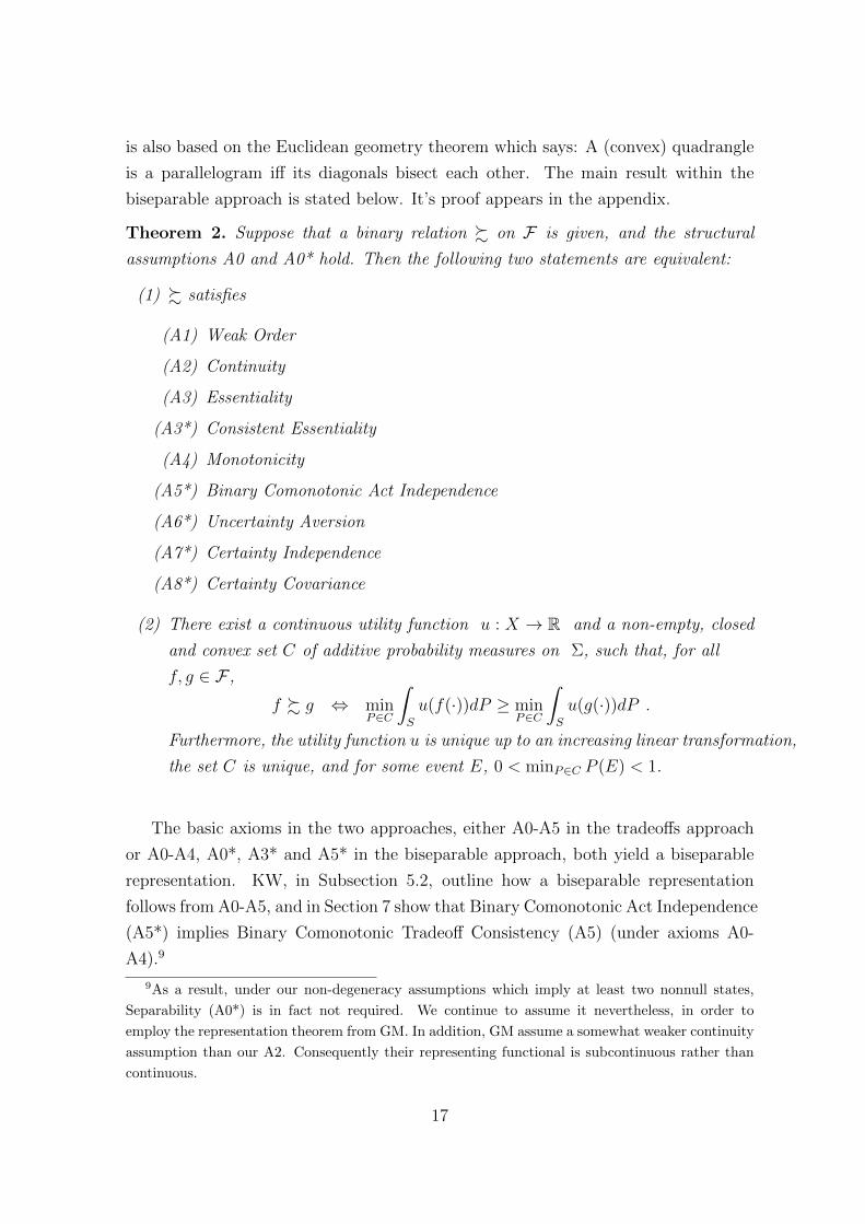
biseparable approach is stated below. It’s proof appears in the appendix.

Theorem 2. Suppose that a binary relation % on F is given, and the structural

assumptions A0 and A0* hold. Then the following two statements are equivalent:

(1) % satisfies

(A1) Weak Order

(A2) Continuity

(A3) Essentiality

(A3*) Consistent Essentiality

(A4) Monotonicity

(A5*) Binary Comonotonic Act Independence

(A6*) Uncertainty Aversion

(A7*) Certainty Independence

(A8*) Certainty Covariance

(2) There exist a continuous utility function u : X → R and a non-empty, closed

and convex set C of additive probability measures on Σ, such that, for all

f, g ∈ F ,

f % g ⇔ minP∈C

∫S

u(f(·))dP ≥ minP∈C

∫S

u(g(·))dP .

Furthermore, the utility function u is unique up to an increasing linear transformation,

the set C is unique, and for some event E, 0 < minP∈C P (E) < 1.

The basic axioms in the two approaches, either A0-A5 in the tradeoffs approach

or A0-A4, A0*, A3* and A5* in the biseparable approach, both yield a biseparable

representation. KW, in Subsection 5.2, outline how a biseparable representation

follows from A0-A5, and in Section 7 show that Binary Comonotonic Act Independence

(A5*) implies Binary Comonotonic Tradeoff Consistency (A5) (under axioms A0-

A4).9

9As a result, under our non-degeneracy assumptions which imply at least two nonnull states,

Separability (A0*) is in fact not required. We continue to assume it nevertheless, in order to

employ the representation theorem from GM. In addition, GM assume a somewhat weaker continuity

assumption than our A2. Consequently their representing functional is subcontinuous rather than

continuous.

17

After assuming the set of basic axioms, the notion of a consequence y being

‘half-way’ between consequences x and z, in the two approaches, amounts to having

u(y) = u(x)/2 + u(z)/2. Axioms A6-A8 or A6*-A8* can then be seen to yield the

same attributes in utiles space, each expressed in its corresponding language.

4 Extensions and Comments

4.1 Bounded acts

Until now we have dealt with finite valued and measurable acts. An obvious question

arises whether the main results hold when the set of acts is extended to include all

measurable bounded acts.

Definition 9. Given a complete and transitive binary relation, % , on X, an act

a : S → X is said to be bounded if there are two consequences, x, y ∈ X s.t. for all

s ∈ S : x % a(s) % y.

Thus, if % is a binary relation on F satisfying A1 (Weak order), bounded acts

are well defined. Furthermore, assuming A0 and A1 (The structural assumption and

weak order), the set,

F b = {f : S → X | f is bounded and measurable w.r.t. Σ}

is well defined. One can ask under what additional conditions the binary relation on

F can uniquely be extended to a binary relation on F b. Assuming that such conditions

are satisfied we denote this extension also by % ⊂ F b ×F b.

Theorem 3. Suppose that A0 holds and % ⊂ F ×F satisfies A1-A8. Then % has a

unique extension to a binary relation on F b, that satisfies the same axioms, and the

representation (2) of Theorem 1 (or Theorem 2) holds for it.

In other words, it suffices to impose the axioms on finite valued acts to get the

representation for bounded acts. The proof of this result derives from Lemma 20 in

the appendix.

4.2 Preference relations admitting CEU and MEU representations

Theorem 4 below is a purely subjective counterpart of a proposition in Schmeidler

(1989), characterizing preference relations representable by both CEU and MEU

18

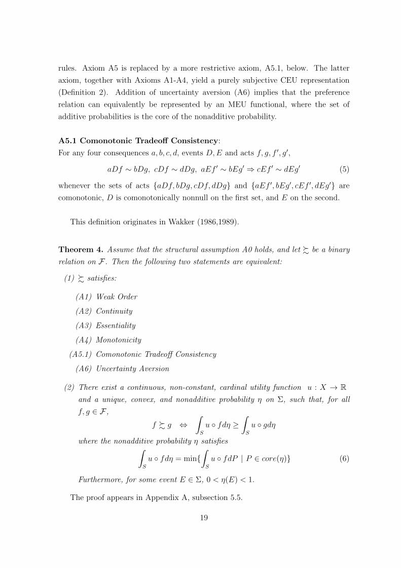
rules. Axiom A5 is replaced by a more restrictive axiom, A5.1, below. The latter

axiom, together with Axioms A1-A4, yield a purely subjective CEU representation

(Definition 2). Addition of uncertainty aversion (A6) implies that the preference

relation can equivalently be represented by an MEU functional, where the set of

additive probabilities is the core of the nonadditive probability.

A5.1 Comonotonic Tradeoff Consistency:

For any four consequences a, b, c, d, events D,E and acts f, g, f ′, g′,

aDf ∼ bDg, cDf ∼ dDg, aEf ′ ∼ bEg′ ⇒ cEf ′ ∼ dEg′ (5)

whenever the sets of acts {aDf, bDg, cDf, dDg} and {aEf ′, bEg′, cEf ′, dEg′} are

comonotonic, D is comonotonically nonnull on the first set, and E on the second.

This definition originates in Wakker (1986,1989).

Theorem 4. Assume that the structural assumption A0 holds, and let % be a binary

relation on F . Then the following two statements are equivalent:

(1) % satisfies:

(A1) Weak Order

(A2) Continuity

(A3) Essentiality

(A4) Monotonicity

(A5.1) Comonotonic Tradeoff Consistency

(A6) Uncertainty Aversion

(2) There exist a continuous, non-constant, cardinal utility function u : X → Rand a unique, convex, and nonadditive probability η on Σ, such that, for all

f, g ∈ F ,

f % g ⇔∫S

u ◦ fdη ≥∫S

u ◦ gdη

where the nonadditive probability η satisfies∫S

u ◦ fdη = min{∫S

u ◦ fdP | P ∈ core(η)} (6)

Furthermore, for some event E ∈ Σ, 0 < η(E) < 1.

The proof appears in Appendix A, subsection 5.5.

19

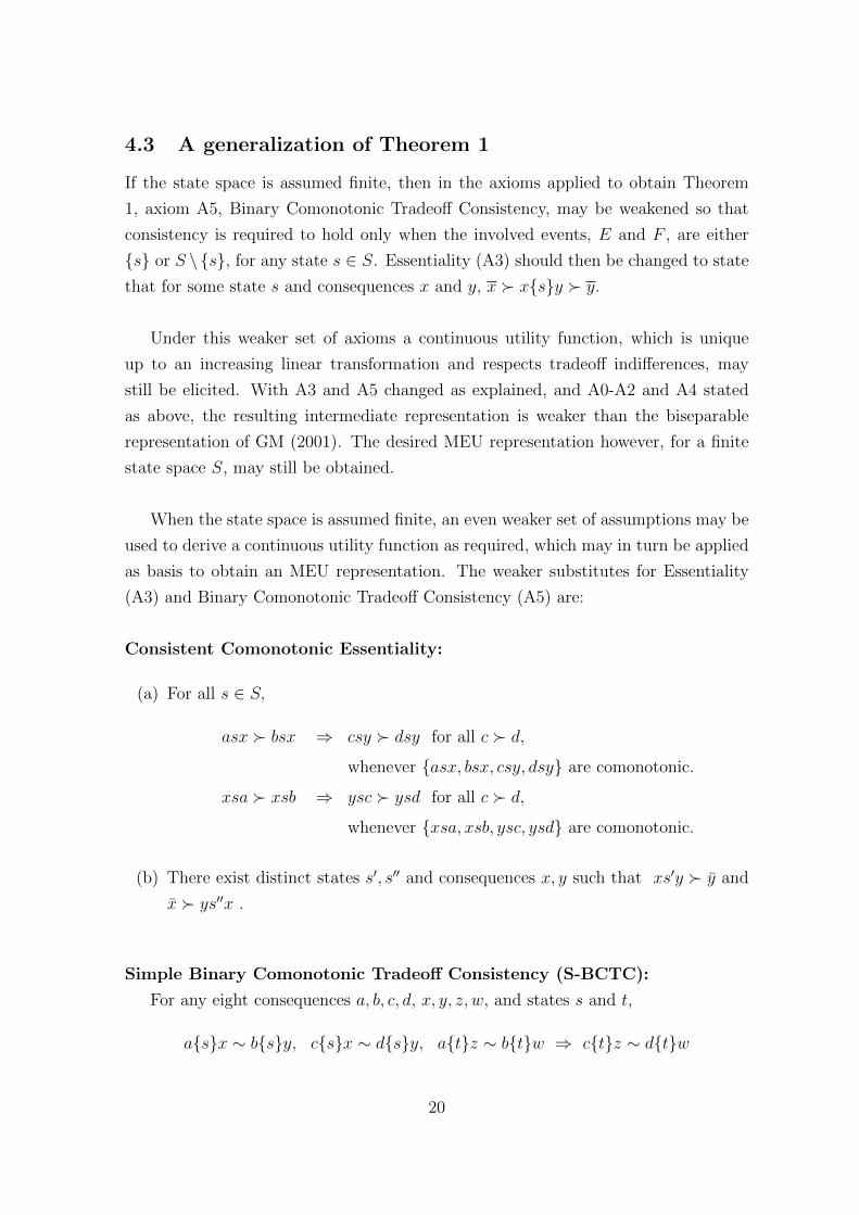
4.3 A generalization of Theorem 1

If the state space is assumed finite, then in the axioms applied to obtain Theorem

1, axiom A5, Binary Comonotonic Tradeoff Consistency, may be weakened so that

consistency is required to hold only when the involved events, E and F , are either

{s} or S \{s}, for any state s ∈ S. Essentiality (A3) should then be changed to state

that for some state s and consequences x and y, x � x{s}y � y.

Under this weaker set of axioms a continuous utility function, which is unique

up to an increasing linear transformation and respects tradeoff indifferences, may

still be elicited. With A3 and A5 changed as explained, and A0-A2 and A4 stated

as above, the resulting intermediate representation is weaker than the biseparable

representation of GM (2001). The desired MEU representation however, for a finite

state space S, may still be obtained.

When the state space is assumed finite, an even weaker set of assumptions may be

used to derive a continuous utility function as required, which may in turn be applied

as basis to obtain an MEU representation. The weaker substitutes for Essentiality

(A3) and Binary Comonotonic Tradeoff Consistency (A5) are:

Consistent Comonotonic Essentiality:

(a) For all s ∈ S,

asx � bsx ⇒ csy � dsy for all c � d,

whenever {asx, bsx, csy, dsy} are comonotonic.

xsa � xsb ⇒ ysc � ysd for all c � d,

whenever {xsa, xsb, ysc, ysd} are comonotonic.

(b) There exist distinct states s′, s′′ and consequences x, y such that xs′y � y and

x � ys′′x .

Simple Binary Comonotonic Tradeoff Consistency (S-BCTC):

For any eight consequences a, b, c, d, x, y, z, w, and states s and t,

a{s}x ∼ b{s}y, c{s}x ∼ d{s}y, a{t}z ∼ b{t}w ⇒ c{t}z ∼ d{t}w

20

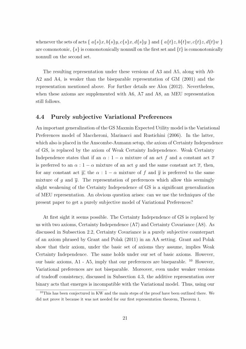
whenever the sets of acts { a{s}x, b{s}y, c{s}x, d{s}y } and { a{t}z, b{t}w, c{t}z, d{t}w }are comonotonic, {s} is comonotonically nonnull on the first set and {t} is comonotonically

nonnull on the second set.

The resulting representation under these versions of A3 and A5, along with A0-

A2 and A4, is weaker than the biseparable representation of GM (2001) and the

representation mentioned above. For further details see Alon (2012). Nevertheless,

when these axioms are supplemented with A6, A7 and A8, an MEU representation

still follows.

4.4 Purely subjective Variational Preferences

An important generalization of the GS Maxmin Expected Utility model is the Variational

Preferences model of Maccheroni, Marinacci and Rustichini (2006). In the latter,

which also is placed in the Anscombe-Aumann setup, the axiom of Certainty Independence

of GS, is replaced by the axiom of Weak Certainty Independence. Weak Certainty

Independence states that if an α : 1 − α mixture of an act f and a constant act x

is preferred to an α : 1 − α mixture of an act g and the same constant act x, then,

for any constant act y, the α : 1 − α mixture of f and y is preferred to the same

mixture of g and y. The representation of preferences which allow this seemingly

slight weakening of the Certainty Independence of GS is a significant generalization

of MEU representation. An obvious question arises: can we use the techniques of the

present paper to get a purely subjective model of Variational Preferences?

At first sight it seems possible. The Certainty Independence of GS is replaced by

us with two axioms, Certainty Independence (A7) and Certainty Covariance (A8). As

discussed in Subsection 2.2, Certainty Covariance is a purely subjective counterpart

of an axiom phrased by Grant and Polak (2011) in an AA setting. Grant and Polak

show that their axiom, under the basic set of axioms they assume, implies Weak

Certainty Independence. The same holds under our set of basic axioms. However,

our basic axioms, A1 - A5, imply that our preferences are biseparable. 10 However,

Variational preferences are not biseparable. Moreover, even under weaker versions

of tradeoff consistency, discussed in Subsection 4.3, the additive representation over

binary acts that emerges is incompatible with the Variational model. Thus, using our

10This has been conjectured in KW and the main steps of the proof have been outlined there. We

did not prove it because it was not needed for our first representation theorem, Theorem 1.

21

method does not enable representation of purely subjective variational preferences.

It still is an open problem.

5 Appendix: The proofs

We begin by listing two observations, which are standard in neoclassical consumer

theory. These observations will be used in the sequel, sometimes without explicit

reference.

Observation 5. Weak order, Substantiality and Monotonicity imply that there are

two consequences x∗, x∗ ∈ X such that x∗ � x∗.

Observation 6. Weak order, Continuity and Monotonicity imply that each act f ∈ Fhas a certainty equivalent, i.e., a constant act x such that f ∼ x.

5.1 Proof of Theorem 1: (1)⇒(2)

Our first step is to use A0 through A5 to derive a cardinal utility function which

represents % on constant acts, that is, a utility function that satisfies that

< a; b > ∼∗< c; d > implies u(a)− u(b) = u(c)− u(d). A representation on F is then

defined using certainty equivalents.

Proposition 7. Under axioms A0 to A5 the following is satisfied:

(1) there exists a continuous function u : X → R such that for all x, y ∈ X,

x % y ⇐⇒ u(x) ≥ u(y), and < a; b > ∼∗< c; d > implies

u(a) − u(b) = u(c) − u(d). Furthermore, u is unique up to a positive linear

transformation.

(2) Given a function u as in (1) there exists a unique continuous J : F → R, such

that for all x ∈ X, J(x) = u(x), and for all f, g ∈ F ,

f % g ⇐⇒ J(f) ≥ J(g) .

5.1.1 Proof of Proposition 7

Let E be an event such that x � xEy � y for some consequences x, y (exists by

Essentiality (A3)). The next claim shows that strict preferences then hold for all

such consequences.

22

Claim 8. Let D be an event and x, y, z consequences such that xDz � yDz and

xDz, yDz are comonotonic. Then αDγ � βDγ whenever α, β, γ are consequences

for which α � β and {αDγ, βDγ, xDz, yDz} is a comonotonic set of acts.

Proof. Assume w.l.o.g. that y % z. Suppose on the contrary that αDγ ∼ βDγ. By

assumption D is comonotonically nonnull on {αDγ, βDγ}. Since obviously αDγ ∼αDγ and αDβ ∼ αDβ (which belongs to the same comonotonic set of acts), then

BCTC (A5) implies that also αDβ ∼ βDβ = β. If Dc is comonotonically null on

{βDcα}, then αDβ = βDcα ∼ αDcα = α. Otherwise, if Dc is comonotonically

nonnull on {βDcα}, then from the three equivalences: αDγ ∼ βDγ, βDγ ∼ βDγ

and βDcα ∼ βDcα, applying BCTC, we conclude αDcα = α ∼ βDcα = αDβ. In

any case, whether Dc is comonotonically null or nonnull as assumed, it is obtained

that α ∼ β. Contradiction. If z % x then the roles of α and β are reversed and the

proof remains the same. �

We define a new decision problem. Define {E,Ec} to be the new state space.

Let X{E,Ec} be the set of acts, functions from the new state space to the set of

consequences X. For consequences a and b, (a, b) denotes an act in X{E,Ec}, assigning

a to E and b to Ec. To avoid confusion, we use the notation (a, b) and (a, a) for acts

in X{E,Ec} and reserve the notation aEb and a for acts in F . Define a binary relation

%E on X{E,Ec} by:

for all (a, b), (c, d) ∈ X{E,Ec},

(a, b) %E (c, d) ⇐⇒ aEb % cEd, aEb, cEd ∈ F .

There exists a one-to-one correspondence between the sets X{E,Ec} and

{ aEb | a, b ∈ X }. Thus, the product topology on X{E,Ec} is equivalent to the

original topology, restricted to the set { aEb | a, b ∈ X }. We summarize some of the

attributes of %E in the next lemma.

Lemma 9. The binary relation %E on X{E,Ec} satisfies Weak order, Continuity,

Monotonicity, Non-nullity of the states E and Ec and (Binary) Comonotonic Tradeoff

Consistency.

Proof. Weak Order, Continuity, Monotonicity and Non-nullity follow from the definition

of %E and the attributes of the original relation %, and from the equivalence between

the topology on X{E,Ec} and the topology on XS restricted to { aEb | a, b ∈ X}.Note that when there are only two states, axioms A5 (Binary Comonotonic Tradeoff

Consistency) and A5.1 (Comonotonic Tradeoff Consistency) coincide. It follows that

23

%E satisfies Comonotonic Tradeoff Consistency. �

Additive representation of %E on X{E,Ec} is obtained using Corollary 10 and

Observation 9 of KW, applied to the case of two states, stated below. Uniqueness

of u and ρ follows from both E and Ec being comonotonically nonnull on the set

{aEb | a % b} (by choice of E). KW use a slightly different tradeoff consistency

condition than ours, however assuming the rest of our axioms their condition follows

(see proof in Subsection 5.6).

Lemma 10. (Corollary 10 and Observation 9 of KW 2003:) Assume the conclusions

of Lemma 9. Then there exists a nonadditive probability ρ on 2{E,Ec} and a continuous

utility function u : X → R, such that %E is represented on X{E,Ec} by the following

CEU functional U :

U((a, b)) =

{u(a)ρ(E) + u(b)[1− ρ(E)] a % b

u(b)ρ(Ec) + u(a)[1− ρ(Ec)] otherwise(7)

Furthermore, u is unique up to an increasing linear transformation and ρ is

unique.

Denote by U the CEU functional over acts of the form aEb, which existence is

guaranteed by the lemma. Let u denote the corresponding utility function and ρ

the corresponding nonadditive probability. The functional U represents % on acts of

the form aEb and the utility function u represents % on X, and is unique up to an

increasing linear transformation. We proceed to show that u is cardinal, in the sense

that tradeoff indifference implies equivalence of utility differences.

Let F 6= E be an event. If F and F c are comonotonically nonnull on some

comonotonic set of the form aFb (either a % b or b % a) then a CEU functional as

in Lemma 10, representing % on acts of the form aFb, may be obtained. The link

between this functional and U is elucidated in the following lemma.

Lemma 11. Let F 6= E, and suppose that F and F c are comonotonically nonnull on

some comonotonic set of the form aFb. Let W be a CEU representation on X{F,Fc}

(according to Lemma 10), and w the corresponding utility function. Then w = σu+τ ,

σ > 0.

Proof. Denote by ϕ the nonadditive probability corresponding to W . Denote, for

x ∈ X, V1(x) = u(x)ρ(E), and recall that ρ(E) > 0, as E is comonotonically nonnull

on {aEb | a % b}. Suppose that F and F c are comonotonically nonnull on {aFb | a %

24

b}, and let W1(x) = w(x)ϕ(F ). Binary Comonotonic Tradeoff Consistency allows us

to follow the steps of Lemma VI.8.2 in Wakker 1989, to obtain W1 = ηV1 + λ, η > 0,

thus w(x) = σu + τ (set σ = ηρ(E)/ϕ(F ) > 0 , where ϕ(F ) > 0 follows from F

being comonotonically nonnull as assumed).

Otherwise, if F and F c are comonotonically nonnull on {aFb | a - b}, the result

may be obtained using a functional W2(x) = w(x)ϕ(F c) (here again ϕ(F c) > 0

because F c is comonotonically nonnull as assumed). �

Corollary 12. For any four consequences a, b, c, d, < a; b > ∼∗< c; d > implies

u(a)− u(b) = u(c)− u(d).

Proof. Let < a; b > ∼∗< c; d >. Then there exist consequences x, y and an event F

such that aFx ∼ bFy and cFx ∼ dFy, with {aFx, bFy, cFx, dFy} comonotonic

and F comonotonically nonnull on this set. Assume first that F c is comonotonically

null on {aFx, bFy, cFx, dFy}. It is next proved that in that case it must be that

a ∼ b and c ∼ d.

Suppose on the contrary that a � b (w.l.o.g.; similar arguments work for the case

b � a). If a % x and b % y, then aFy, bFy are comonotonic, and by nullity of F c on

the comonotonic set involved, aFx ∼ aFy ∼ bFy, and obviously also aFy ∼ aFy,

where F is assumed to be comonotonically nonnull on the comonotonic set of acts

{aFy, bFy}. If a - x and b - y, then similarly aFx, bFx are comonotonic, and by

nullity of F c on the comonotonic set involved, aFx ∼ bFy ∼ bFx, and also aFx ∼aFx, where F is comonotonically nonnull on the comonotonic set of acts {aFx, bFx}.In any case, it is also true that aEb ∼ aEb, where E is comonotonically nonnull on the

set of acts containing aEb. By Binary Comonotonic Tradeoff Consistency it follows

that aEb ∼ bEb = b, contradicting Claim 8. Therefore it must be that a ∼ b. The

same can be proved for the consequences c and d. Thus, if F c is comonotonically null

on the set of acts {aFx, bFy, cFx, dFy}, then the above indifference relations imply

a ∼ b and c ∼ d, resulting trivially u(a)− u(b) = 0 = u(c)− u(d).

Suppose now that F c is comonotonically nonnull on the relevant binary comonotonic

set. According to Lemma 10 there exists a CEU representation over acts of the

form aFb, with a utility function unique up to an increasing linear transformation,

and a unique nonadditive probability. Denote the CEU functional by W , with a

corresponding utility function w. The indifference relations aFx ∼ bFy and

cFx ∼ dFy then imply w(a) − w(b) = w(c) − w(d). If F = E or F = Ec then

by the uniqueness result in Lemma 10, w = σu+ τ with σ > 0. If F is another event,

25

then Lemma 11 yields this relation. In any case, w(a)− w(b) = w(c)− w(d) implies

u(a)− u(b) = u(c)− u(d). �

The next lemma establishes the uniqueness of u.

Lemma 13. u is unique up to a positive linear transformation.

Proof. Let u be some other representation of % on X, which satisfies that if <

a; b > ∼∗< c; d > then u(a)− u(b) = u(c)− u(d). Both u and u represent % on X,

therefore u = ψ ◦ u, where ψ is continuous and strictly increasing.

Non-triviality of %, connectedness of X and continuity of u imply that u(X) is a

non-degenerate interval. Let ξ be an internal point of u(X). There exists an interval

R small enough around ξ such that, for all u(a), u(c) and u(b) = [u(a) +u(c)]/2 in R,

there are x, y ∈ X for which aEx, bEy, bEx, cEy are comonotonic, with a % x, b %

y, b % x and c % y, and

u(a)− u(b) = (u(y)− u(x))1− ρ(E)

ρ(E)= u(b)− u(c).

That is, aEx ∼ bEy and bEx ∼ cEy, with {aEx, bEy, bEx, cEy} comonotonic,

which is precisely the definition of < a; b > ∼∗< b; c >. By the assumption on u,

u(a) − u(b) = u(b) − u(c), which in fact implies that for all α, γ ∈ R , ψ satisfies

ψ((α + γ)/2) = [ψ(α) + ψ(γ)]/2. By Theorem 1 of section 2.1.4 of Aczel (1966), ψ

must be a positive linear transformation. �

Statement (1) of Proposition 7 is proved. Having a specific u, a unique representation

J on F follows using certainty equivalents. By Observation 6 there exists, for any

f ∈ F , a constant act CE(f) such that f ∼ CE(f). Set J(f) = u(CE(f)), then for

all f, g ∈ F ,

f % g ⇐⇒ CE(f) % CE(g) ⇐⇒ J(f) = u(CE(f)) ≥ u(CE(g)) = J(g)

That is, J represents % on F . J is unique and continuous by its definition and by

continuity of u. The proof of the proposition is completed.

5.2 Proof of the implication (1)⇒(2) of Theorem 1 - continued

Throughout this subsection E will denote an event that satisfies x � xEy � y

whenever x � y (exists by Essentiality and Claim 8), and U will denote the CEU

representation on binary acts of the form aEb (according to Lemma 10). u and ρ

26

will notate the corresponding utility function on X and nonadditive probability on

2{E,Ec}, respectively. By choice of E, 0 < ρ(E) < 1. As proved above, u satisfies

(1) of Proposition 7, and we denote by J the representation of % over F obtained

according to (2) of the proposition. By connectedness of X and continuity of u, u(X)

is an interval. Since u is unique up to a positive linear transformation, we fix it for

the rest of this proof such that there are x∗, x∗ for which u(x∗) = −2 and u(x∗) = 2.

θ is a consequence such that u(θ) = 0.

The proof is conducted in three logical steps. First, an MEU representation is

obtained on a subset of F . This is done by moving to work in utiles space, and

applying tools from GS. Afterwards, the representation is extended to a ’stripe’, in

utiles space, around the main diagonal. The last step extends the representation to

the entire space.

Claim 14. There exists a subset Y ⊂ X such that u(Y ) is a non-degenerate interval,

θ ∈ Y , and for all a, b, c, d ∈ Y , u(a)−u(b) = u(c)−u(d) implies < a; b > ∼∗< c; d >.

Proof. Employing the representation U and Continuity of u, there exists an interval

[−τ, τ ] (0 < τ) small enough such that if u(a), u(b), u(c), u(d) ∈ [−τ, τ ] satisfy

u(a)− u(b) = u(c)− u(d), there are x, y ∈ X for which u(x), u(y) ≤ −τ and

u(a)− u(b) =1− ρ(E)

ρ(E)[u(y)− u(x)] = u(c)− u(d).

It follows that aEx ∼ bEy and cEx ∼ dEy. By choice of the consequences and

the event E, the set {aEx, bEy, cEx, dEy} is comonotonic and E is comonotonically

nonnull on this set. Thus < a; b > ∼∗< c; d >.

Let Y = {y ∈ X | u(y) ∈ [−τ, τ ]}. Y is a subset of X, u(Y ) is an interval, θ ∈ Y ,

and for all a, b, c, d ∈ Y , u(a)− u(b) = u(c)− u(d) implies < a; b > ∼∗< c; d >. �

Throughout this subsection Y will denote a subset of X as specified in the above

claim. Note that utility mixtures of acts in Y S are also in Y S (this fact is employed

in the proof without further mention).

The following is a utilities analogue to Schmeidler’s (1989) uncertainty aversion

axiom.

A6u. Uncertainty Aversion in Utilities:

27

Let the preference relation % be represented on constant acts by a utility function u.

If f, g, h are acts such that f % g , and for all states s, u(h(s)) = 12u(f(s))+ 1

2u(g(s)),

then h % g.

Lemma 15. If (1) of the theorem holds then Uncertainty Aversion in Utilities (A6u)

is satisfied on F ∩ Y S.

Proof. Let f, g, h ∈ F ∩ Y S be acts satisfying f % g, h such that in all states s,

u(h(s)) = 12u(f(s)) + 1

2u(g(s)). Then for all states s,

u(f(s))− u(h(s)) = u(h(s))− u(g(s)), therefore < f(s), h(s) > ∼∗< h(s), g(s) >. By

A6 it follows that h % g. �

Comment 16. Applying A6u consecutively implies that if f, g, h ∈ F ∩ Y S are acts

satisfying f % g, h an act such that for all states s,

u(h(s)) = k2mu(f(s)) + (1 − k

2m)u(g(s)), ( k

2m∈ [0, 1]) then h % g. Continuity then

yields that the same is true for any α : 1− α utilities mixture (α ∈ [0, 1]).

Claim 17. Let f ∈ F∩Y S be an act, x ∈ F∩Y S a constant act such that f ∼ x, and

α ∈ (0, 1). If g is an act such that for all states s, u(g(s)) = αu(f(s)) + (1− α)u(x),

then g ∼ x.

Proof. We first prove the claim for α = 12m

, that is, when g satisfies, for all states s,

u(g(s)) = 12mu(f(s)) + (1 − 1

2m)u(x). The proof is by induction on m. For m = 1,

in all states s, < f(s); g(s) > ∼∗< g(s);x >, which by certainty independence (A7)

(with w = x) implies g ∼ x. Assume that for g that satisfies

u(g(s)) = 12mu(f(s)) + (1− 1

2m)u(x), g ∼ x. Let h be an act such that

u(h(s)) = 12m+1u(f(s)) + (1− 1

2m+1 )u(x). The act h satisfies, for all states s,

u(h(s)) = 12u(g(s)) + 1

2u(x), and g ∼ x by the induction assumption. Employing

Certainty Independence again implies h ∼ x.

Now let α = k2m

(k ∈ {2, . . . , 2m − 1}). For all states s,

u(g(s)) = k2mu(f(s)) + (1 − k

2m)u(x). By Uncertainty Aversion in Utilities (A6u),

g % x. We assume g � x and derive a contradiction.

Let g′ be such that u(g′(s)) = 12u(g(s)) + 1

2u(x) for all states s, y a constant act

such that g ∼ y. For all states s, u(g(s)) ∈ u(Y ), and u(Y ) is an interval, therefore

by Monotonicity and Essentiality u(y) ∈ u(Y ). Employing Certainty Independence,

g′ ∼ z for z such that u(z) = u(x)+u(y)2

> u(x), so g′ � x. However, There exists an

28

act h such that u(h(s)) = j2nu(g(s)) + (1− j

2n)u(g′(s)) and also

u(h(s)) = 12mu(f(s))+(1− 1

2m)u(x) for some j, n,m ∈ N. By the previous paragraph,

h ∼ x. But Uncertainty Aversion in Utilities requires that h % g′, contradiction.

Therefore if g satisfies u(g(s)) = k2mu(f(s))+(1− k

2m)u(x) for all states s, then g ∼ x.

By continuity it follows that the same is true for any α ∈ (0, 1) . �

Claim 18. Let f ∈ F ∩ Y S be an act, w, x, y ∈ F ∩ Y S constant acts and α ∈ (0, 1),

such that f ∼ x and u(y) = αu(x) + (1−α)u(w). If h is an act such that in all states

s, u(h(s)) = αu(f(s)) + (1− α)u(w), then h ∼ y.

Proof. Let g be an act such that for all states s, u(g(s)) = αu(f(s)) + (1 − α)u(x),

then g ∈ F ∩ Y S. For all states s,

u(h(s)) = αu(f(s)) + (1− α)u(w) = u(g(s)) + u(y)− u(x)⇐⇒u(h(s))− u(g(s)) = u(y)− u(x) ⇐⇒< h(s); g(s) > ∼∗< y;x > .

According to Claim 17, g ∼ x, therefore by Certainty Covariance h ∼ y. �

The following is an analogue to Lemma 3.3 from GS, and follows the lines of the

proof given there. Denote by B0 the set of real-valued functions on S which assume

finitely many values, and by B the space of all bounded Σ-measurable real-valued

functions on S. For any γ ∈ R, γ ∈ B0 is the constant function γS.

Lemma 19. There exists a functional I : B0 → R such that:

(i) For f ∈ F ∩ Y S, I(u ◦ f) = J(f).

(ii) I is monotonic (i.e., for a, b ∈ B0, if a ≥ b then I(a) ≥ I(b)).

(iii) I is superadditive and homogeneous of degree 1 (therefore I(1) = 1).

(iv) I satisfies certainty independence: for any a ∈ B0 and γ a constant function,

I(a+ γ) = I(a) + I(γ).

Proof. For a ∈ B0 ∩ (u(Y ))S define I(a) by (i). By monotonicity, if in all states s,

f(s) ∼ g(s), then f ∼ g. I is therefore well defined.

29

We show that I is homogeneous on B0 ∩ (u(Y ))S. Let a, b ∈ B0 ∩ (u(Y ))S,

b = αa. Let f, g be acts such that u ◦ f = a, u ◦ g = b, and x, y ∈ X such

that f ∼ x, u(y) = αu(x). Monotonicity and the fact that Y contains θ imply

that x, y ∈ F ∩ Y S. Applying Claim 18 with w = θ implies that g ∼ y. Thus

I(b) = J(g) = u(y) = αu(x) = αJ(f) = αI(a), and homogeneity is established.

The functional I may now be extended from B0 ∩ (u(Y ))S to B0 by homogeneity.

By its definition, I is homogeneous on B0, and by monotonicity of the preference

relation I is also monotonic. Note also that if y ∈ Y and u(y) = γ, then I(γ) =

u(y) = γ, and homogeneity implies that I(1) = 1. Again by homogeneity it suffices

to show that certainty independence and superadditivity of I hold on B0 ∩ (u(Y ))S.

For certainty independence, let a, γ ∈ B0 ∩ (u(Y ))S. Let f ∈ F ∩Y S be such that

u◦f = a, and denote I(a) = β. Suppose x, y, w ∈ F ∩Y S are constant acts such that

u(x) = β, u(w) = γ, u(y) = (u(x) + u(w))/2 and h an act such that in all states s,

u(h(s)) = 12(u(f(s)) + u(w)). Then h ∈ F ∩ Y S, f ∼ x, and by Claim 18 it follows

that h ∼ y, which implies

J(h) = I(u ◦ h) = I(1

2(u ◦ f + γ)) = u(y) =

1

2(β + γ) =

1

2(I(a) + γ).

Hence, using homogeneity to extend the result to B0, for all a, γ ∈ B0,

I(a+ γ) = I(a) + I(γ).

Finally we show that I is superadditive on B0 ∩ (u(Y ))S. Let a, b ∈ B0 ∩ (u(Y ))S

and f, g ∈ F ∩ Y S such that u ◦ f = a, u ◦ g = b. Assume first that I(a) = I(b). By

Lemma 15, if h is an act such that u ◦ h = 12(u ◦ f + u ◦ g), then h % g. Thus,

J(h) = I(u ◦ h) = I(1

2(u ◦ f + u ◦ g)) ≥ J(g) =

1

2(I(a) + I(b)).

so by homogeneity, if a, b ∈ B0 satisfy I(a) = I(b) then I(a+ b) ≥ I(a) + I(b).

Now assume that I(a) > I(b) and let γ = I(a) − I(b), c = b + γ. Certainty

independence of I implies I(c) = I(b) + γ = I(a). Again by certainty independence

and by superadditivity for the case I(a) = I(b), it follows that

I(1

2(a+ b)) +

1

2γ = I(

1

2(a+ c)) ≥ 1

2(I(a) + I(c)) =

1

2(I(a) + I(b)) +

1

2γ.

30

and superadditivity is proved for all a, b ∈ B0 ∩ (u(Y ))S, and may be extended to B0

using homogeneity. �

Lemmas 3.4 and 3.5 from GS may now be applied to obtain an MEU representation

of % on F ∩ Y S.

Lemma 20. (Lemma 3.4 from GS):

There exists a unique continuous extension of I to B, and this extension is monotonic,

superlinear and C-independent.

Lemma 21. (Lemma 3.5 and an implied uniqueness result from GS):

If I is a monotonic superlinear certainty-independent functional on B, satisfying

I(1) = 1, there exists a closed and convex set C of finitely additive probability measures

on Σ such that for all b ∈ B, I(b) = min{∫bdP | P ∈ C}. The set C is unique.

Corollary 22. % is represented on F ∩ Y S by an MEU functional.

Let C denote the set of additive probability measures on Σ, involved in the

MEU representation of % on F ∩ Y S. For all f ∈ F ∩ Y S, J(f) = I(u ◦ f) =

min{∫u ◦ fdP | P ∈ C}. Outside of B0 ∩ (u(Y ))S, I is extended by homogeneity.

By the above lemmas, I is monotonic, superadditive, homogeneous of degree 1 and

satisfies certainty independence.

It is now required to show that the homogeneous extension of I outside of

B0 ∩ (u(Y ))S is consistent with the preference relation. That is, that for all f ∈ F ,

J(f) = I(u◦f) = min{∫u◦fdP | P ∈ C} . The proof consists of two steps. First, the

representation is extended to a ‘stripe’ (in utiles space) parallel to the main diagonal,

obtained by ‘sliding’ B0 ∩ (u(Y ))S along the diagonal. Then the representation is

further extended from that stripe to the entire space.

For an act g ∈ F , let diag(g) = {f ∈ F | u ◦ f = u ◦ g + γ, γ ∈ R}. That is,

diag(g) contains all acts that can be obtained from g by constant shifts (translations

parallel to the main diagonal, in utiles space). Note that diag(g) is convex w.r.t.

utility mixtures.

Claim 23. Let g ∈ F ∩ Y S. Then for all acts f ∈ diag(g), J(f) = I(u ◦ f).

Proof. Let f, g be acts that satisfy g ∈ F ∩ Y S and u ◦ f = u ◦ g + ε , ε > 0, so

f ∈ diag(g). Suppose that x, y are consequences such that g ∼ y and u(x)−u(y) = ε.

31

It follows that for all states t, u(f(t))− u(g(t)) = u(x)− u(y).

Similarly to the proof of Claim 14, if ε is small enough then there are z1, z2 such

that u(z1), u(z2) < mins u(g(s)), and (recall that ρ(E) > 0)

ε = u(f(s))− u(g(s)) =1− ρ(E)

ρ(E)[u(z2)− u(z1)] = u(x)− u(y)

It follows that for all consequences f(s) and g(s), f(s)Ez1 ∼ g(s)Ez2 and xEz1 ∼yEz2, with {f(s)Ez1, g(s)Ez2, xEz1, yEz2} comonotonic, and E comonotonically nonnull

on this set. Thus < f(s); g(s) > ∼∗< x; y > for all states s. Certainty Covariance

implies f ∼ x. Applying certainty independence of I,

I(u ◦ f + u ◦ y) = I(u ◦ f) + u(y) = I(u ◦ g + u ◦ x) = J(g) + u(x),

and I(u ◦ f) = u(x) = J(f). The same procedure may be repeated (in small ’tradeoff

steps’) for all f ∈ diag(g) that satisfy u◦f = u◦g+γ, γ ≥ 0, to obtain J(f) = I(u◦f).

In order to extend the representation to the lower part of the diagonal, let f, g be

acts that satisfy g ∈ F ∩ Y S and u ◦ f = u ◦ g − ε , ε > 0. Let x, y be consequences

such that g ∼ y and u(y) − u(x) = ε. Similarly to the previous case, if ε is small

enough then there are z3, z4 such that u(z3), u(z4) > maxu(g(s)) and (recall that

ρ(E) < 1)

ε = u(g(s))− u(f(s)) =ρ(E)

1− ρ(E)[u(z3)− u(z4)] = u(y)− u(x)

It follows that for all consequences f(s) and g(s), f(s)Ecz3 ∼ g(s)Ecz4 and

xEcz3 ∼ yEcz4, with the set {f(s)Ecz3, g(s)Ecz4, xEcz3, yE

cz4} comonotonic, and

Ec comonotonically nonnull on this set. Therefore < f(s); g(s) > ∼∗< x; y > for all

states s. By Certainty Covariance it follows that f ∼ x, and certainty independence

of I again implies that J(f) = I(u ◦ f). Subsequent applications yield the result for

all acts f such that u ◦ f = u ◦ g − γ, γ ≥ 0, and the proof is completed. �

Claim 22 implies that J(f) = min{∫u ◦ fdP | P ∈ C} for all f ∈ F that satisfy

u ◦ f = u ◦ g + γ for some g ∈ F ∩ Y S and γ ∈ R. That is, % is represented by

an MEU functional in a ’stripe’ containing all acts with utilities in [−τ, τ ], and those

obtained from them by translations parallel to the main diagonal (in utiles space).

32

To complete the proof and show that the MEU representation holds for all acts, an

auxiliary result is proved. It consists of showing that for any subset of consequences

there exists a consequence ξ that has a tradeoff-midpoint with every intermediate

consequence (including the extreme ones, if those exist).

Claim 24. Let m,M ∈ u(X) be such that m < M . Then there exists a consequence

ξ ∈ X, m < u(ξ) < M , such that for all x ∈ X with m ≤ u(x) ≤ M , there is y ∈ Xthat satisfies

< x; y > ∼∗< y; ξ >

Proof. Choose a consequence ξ ∈ X such that u(ξ) = ρ(E)M + (1 − ρ(E))m. By

continuity of u and connectedness of X, the definition of M and m and the fact

that 0 < ρ(E) < 1, such a consequence exists, and its utility is strictly between M

and m. To show that every x ∈ X with utility (weakly) between M and m has

a tradeoff-midpoint with ξ, the cases u(x) ≥ u(ξ) and u(ξ) > u(x) are examined

separately.

Suppose first that u(ξ) ≤ u(x) ≤ M . In order to show that there exists y that

satisfies < x; y > ∼∗< y; ξ > it suffices to show that there are consequences a, b which

satisfy u(ξ) ≥ u(b) ≥ u(a) > m, and xEa ∼ yEb, yEa ∼ ξEb. For that, using the

CEU representation over binary acts contingent on E, it suffices to prove that there

are a, b ∈ X for which,

u(x)ρ(E) + u(a)[1− ρ(E)] =u(x) + ρ(E)M + (1− ρ(E))m

2ρ(E) + u(b)[1− ρ(E)] ,

where M ≥ u(x) ≥ u(ξ) ≥ u(b) ≥ u(a) ≥ m, or, rearranging the above expression,

u(b)− u(a) =ρ(E)

2(1− ρ(E))[u(x)− ρ(E)M − (1− ρ(E))m]

with M ≥ u(x) ≥ u(ξ) ≥ u(b) ≥ u(a) > m. By continuity of u and connectedness

of X, such u(b)− u(a) obtains all values from zero up to u(ξ)−m = ρ(E)(M −m).

Thus, it is enough to prove,

ρ(E)

2(1− ρ(E))[u(x)− ρ(E)M − (1− ρ(E))m] ≤ ρ(E)(M −m) ⇐⇒

u(x)− ρ(E)M − (1− ρ(E))m ≤ 2(1− ρ(E))M − 2(1− ρ(E))m ⇐⇒u(x) ≤ ρ(E)M + 2(1− ρ(E))M − (1− ρ(E))m = M + (1− ρ(E))(M −m) .

As by assumption u(x) ≤ M and M > m, this condition is satisfied, and a

tradeoff-midpoint of ξ and any x ∈ X with u(ξ) ≤ u(x) ≤M exists as required.

33

Next suppose that x ∈ X satisfiesm ≤ u(x) < u(ξ). Similarly to the previous case,

it suffices to show that there are consequences c, d which satisfy M ≥ u(d) ≥ u(c) ≥u(ξ), and ξEcc ∼ yEcd, yEcc ∼ xEcd. Using once more the CEU representation over

binary acts contingent on E, it suffices to prove that there are c, d ∈ X for which

u(d)ρ(E) + u(x)[1− ρ(E)] = u(c)ρ(E) +u(x) + ρ(E)M + (1− ρ(E))m

2[1− ρ(E)]

where M ≥ u(d) ≥ u(c) ≥ u(ξ) > u(x) ≥ m, or, rearranging the above expression,

u(d)− u(c) =1− ρ(E)

2ρ(E)[ρ(E)M + (1− ρ(E))m− u(x)]

with M ≥ u(d) ≥ u(c) ≥ u(ξ) > u(x) ≥ m. By continuity of u and connectedness of

X, u(d)−u(c) obtains all values in the range [0,M −u(ξ)] = [0, (1− ρ(E))(M −m)].

Thus, it is enough to prove,

1− ρ(E)

2ρ(E)[ρ(E)M + (1− ρ(E))m− u(x)] ≤ (1− ρ(E))(M −m) ⇐⇒

ρ(E)M + (1− ρ(E))m− u(x) ≤ 2ρ(E)M − 2ρ(E)m ⇐⇒u(x) ≥ m− ρ(E)(M −m)

which is again true based on the assumptions that u(x) ≥ m and M > m. �

Corollary 25. For all f ∈ F , J(f) = I(u ◦ f).

Proof. As stated above, by claims 22 and 23, % is represented by an MEU functional

on a ’stripe’ containing all acts with utilities in [−τ, τ ], and those obtained from them,

in utiles space, by translations parallel to the main diagonal. It is left to show that

J(f) = I(u ◦ f) for all acts outside that stripe as well.

Let f, g ∈ F be acts and x, y, ξ consequences such that: f is not a constant act,

J(g) = I(u ◦ g), < f(s); g(s) > ∼∗< g(s); ξ > for all states s, g ∼ y and < x; y >

∼∗< y; ξ >. The existence of the required ξ is guaranteed by applying Lemma 24 to

M = maxs∈S u(f(s)) and m = mins∈S u(f(s)) (x such that u(y) = (u(x) + u(ξ))/2

must satisfy m ≤ u(x) ≤M). Employing the axiom of Certainty Independence (A7)

it may be asserted that f ∼ x. Thus, by homogeneity and certainty independence of

I,

u(y) = I(u ◦ g) =1

2(I(u ◦ f) + u(ξ)) =

1

2(I(u ◦ f) + 2u(y)− u(x))

34

and I(u ◦ f) = u(x) = J(f).

In that manner the MEU representation that applies in the stripe may be extended

to any act in F which has a tradeoff-midpoint inside the stripe. By repeating this

procedure, the MEU representation is seen to apply to the entire acts space. �

It is concluded that for all f ∈ F , J(f) = min{∫u ◦ fdP | P ∈ C}, that is, %

on F is represented by an MEU functional, with a utility function unique up to an

increasing linear transformation, and a unique set of prior probabilities C.

The fact that for some event E, 0 < minP∈C P (E) < 1, follows from Essentiality:

the event which existence is guaranteed by Essentiality should satisfy that

x � xEy � y for x � y. Translating to the MEU representation yields

u(x) > u(x) minP∈C P (E) + u(y)(1−minP∈C P (E)) > u(y), hence

0 < minP∈C P (E) < 1. The proof of the direction (1)⇒(2) of the main theorem is

completed.

5.3 Proof of the implication (2)⇒(1) of Theorem 1

By definition of the representation on F , % is a weak order, satisfying Monotonicity.

Define a functional I : B0 → R by I(b) = min{∫SbdP | P ∈ C}. Hence the preference

relation is represented by J(f) = I(u ◦ f). By its definition, I is continuous and

superlinear, therefore % is continuous and satisfies Uncertainty Aversion in Utilities

(A6u). Uncertainty aversion (A6) results by observing that

< f(s), h(s) > ∼∗< h(s), g(s) > implies u(h(s)) = 12[u(f(s)) + u(g(s))].

To see that Essentiality holds let E be an event such that

0 < minP∈C P (E) < 1, and take x � y, which must exist according to the uniqueness

result. Then u(x) = J(x) > u(x) minP∈C P (E)+u(y)(1−minP∈C P (E)) = J(xEy) >

u(y) = J(y).

Next it is proved that Certainty Independence is satisfied. If γ ∈ R and γ is the

constant function returning γ in every state, then for all b ∈ B0,

I(b+ γ) = I(b) + I(γ) = I(b) + γ. If α > 0 then I(αb) = αI(b). Let f, g be acts and

ξ, x, y consequences that satisfy: for all states s, < f(s), g(s) > ∼∗< g(s), ξ > and

< x; y > ∼∗< y; ξ >. Then u(g(s)) = 12[u(f(s)) + u(ξ)] and u(y) = 1

2[u(x) + u(ξ)].

35

Therefore,

J(g) = I(u ◦ g) =1

2I(u ◦ f) +

1

2u(ξ) =

1

2J(f) +

1

2u(ξ)

and J(f) = u(x) ⇔ J(g) = u(y), that is, f ∼ x ⇔ g ∼ y, as required.

To see that Certainty Covariance (A8) holds let f, g be acts and x, y consequences

such that for all states s, < f(s); g(s) > ∼∗< x; y >. Then for all states s,

u(f(s)) − u(g(s)) = u(x) − u(y), which implies I(u ◦ f) + u(y) = I(u ◦ g) + u(x)

and thus f ∼ x ⇔ g ∼ y.

Finally, under MEU, sets of binary comonotonic acts are EU-sets, hence binary

comonotonic tradeoff consistency is satisfied.

5.4 Proof of Theorem 2

By Theorem 11 in GM (2001), assuming A0 and A0*, the binary relation % satisfies

axioms A1,A2,A3,A3*,A4 and A5* if and only if there exist a real valued, continuous,

monotonic and nontrivial representation J : F −→ R of %, and a monotonic set

function η on events, such that for binary acts with x % y,

J(xEy) = u(x)η(E) + u(y)(1− η(E)). (8)

The function u is defined on X by, u(x) = J(x), and it represents % on X. The set

function η, when normalized s.t. η(S) = 1, is unique, and u and J are unique up to

a positive multiplicative constant and an additive constant.

It remains to show that addition of axioms A6*,A7* and A8* yields an MEU

representation as in (2) of the theorem. This is done simply by showing that when

these axioms are translated into utiles space, they imply the exact same attributes

as their counterpart axioms A6, A7 and A8. The key result is Proposition 1 of

Ghirardato et al. (2003), which states that for biseparable preference relations, and

x � y � z in X, y ∈ H(x, z) if and only if u(y) = u(x)/2 + u(z)/2. Applying that

result, we obtain equivalence between A6*, A7* and A8*, and their utilities-analogue

axioms. First, axiom A6* is equivalent to Uncertainty Aversion in Utilities (A6u), as

phrased above. Second, A7* is equivalent to the following utilities-based axiom:

A7u. Certainty Independence in Utilities:

Let the preference relation % be represented on constant acts by a utility function

36

u. Suppose that two acts, f and g, and three consequences, x, y and w, satisfy:

u(y) = 12u(x) + 1

2u(w), and for all states s, u(g(s)) = 1

2u(f(s)) + 1

2u(w). Then

f ∼ x ⇔ g ∼ y.

Finally, A8* is equivalent to the utilities axiom:

A8u. Certainty Covariance in Utilities:

Let f, g be acts and x, y consequences such that ∀s ∈ S :12u(f(s)) + 1

2u(y) = 1

2u(g(s)) + 1

2u(x). Then f ∼ x iff g ∼ y.

Having these utilities axioms (which immediately apply to the entire acts space,

as opposed to the tradeoffs case), the rest of the proof (both directions) is identical

to the proof of Theorem 1.

5.5 Proof of Theorem 4

To obtain a CEU representation on simple acts we apply Corollary 10 from KW,

stated below, supplemented with their subsection 5.1, which extends the theorem to

infinite state spaces. As in the proof of Theorem 1, here as well KW use a slightly

different tradeoff consistency condition than ours. However, assuming the rest of our

axioms, their condition follows (see proof in Subsection 5.6).

Lemma 26. (Corollary 10 of KW 2003, extended to an infinite state space in their

subsection 5.1:) Given a binary relation % on F , the following two statements are

equivalent:

(1) % satisfies:

(A1) Weak Order

(A2) Continuity

(A4) Monotonicity

(A5.1) Comonotonic Tradeoff Consistency

(2) There exist a continuous utility function u : X → R and a nonadditive

probability v on Σ such that, for all f, g ∈ F ,

f % g ⇔∫S

u ◦ fdv ≥∫S

u ◦ gdv

37

Claim 27. If, in addition to axioms A1,A2,A4 and A5.1, Essentiality is satisfied,

then u is cardinal and v is unique and satisfies 0 < v(E) < 1 for some event E.

In the other direction, assuming that u is cardinal, and that v is unique and

satisfies 0 < v(E) < 1 for some event E, Essentiality holds.

Proof. Suppose that Essentiality is satisfied. By Observation 9 of KW, the utility

function u is cardinal, and the nonadditive probability function v is unique. Applying

the CEU representation obtains that there exists an event E for which 0 < v(E) < 1.

Now assume that u is cardinal and v unique, satisfying that for some event E,

0 < v(E) < 1. First, cardinality of u guarantees that there exist consequences x and

y such that x � y. In addition, for the event E, x � xEy � y, thus Essentiality

holds. �

Let u be the utility function and v the non-additive probability obtained by Lemma

26. The proof of the theorem continues in subsections 5.5.1 and 5.5.2 below.

5.5.1 Proof of the implication (1)⇒(2) of Theorem 4.

It is left to prove that addition of Uncertainty Aversion yields the specific CEU form

in (6) (along with the detailed attributes of v).

Lemma 28. Let % satisfy (1) of Lemma 26. Then Uncertainty Aversion (A6)

implies Uncertainty Aversion in Utilities (A6u).

Proof. Let f, g, h be such that f % g, and for all states t,

u(h(t)) = 12u(f(t)) + 1

2u(g(t)). It is proved that h % g.

Let x be an internal consequence, that is, x∗ � x � x∗ for some x∗, x∗. Since X is

connected and u continuous, there exist acts f ′, g′, h′ such that, in all states s,

u(f ′(t)) =1

2nu(f(t)) + (1− 1

2n)u(x)

u(g′(t)) =1

2nu(g(t)) + (1− 1

2n)u(x)

u(h′(t)) =1

2nu(h(t)) + (1− 1

2n)u(x) =

1

2u(f ′(t)) +

1

2u(g′(t))

38

By definition of the CEU functional, f % g ⇔ f ′ % g′ and h % g ⇔ h′ % g′.

Therefore it suffices to prove that h′ % g′.

In order to use Uncertainty Aversion we need to show that for every state t,

< f ′(t);h′(t) > ∼∗< h′(t); g′(t) >. That is, it should be proved that for every

state t there are consequences y, z and an event E such that f ′(t)Ey ∼ h′(t)Ez and

h′(t)Ey ∼ g′(t)Ez. It is next shown that these indifference relations may be satisfied

for an event E such that x � xEy � y whenever x � y (exists by Essentiality and

Claim 8), and f ′, g′, h′ are made ’close enough’ to the internal consequence x.

Let E be an event such that x � xEy � y whenever x � y. By the CEU

representation it follows that 0 < v(E) < 1. Let z1 � z2 � z3 be internal consequences

that satisfy

z1 � x � z2 and u(z1)− u(z2) <2(1− v(E))

v(E)(u(z2)− u(z3))

For any two consequences a � c between z1 and z2, u(a) − u(c) ≤ u(z1) − u(z2).

Thus, applying continuity of u, there are consequences y, z such that

z2 � z � y � z3 and u(a)− u(c) =2[1− v(E)]

v(E)(u(z)− u(y)).

Rearranging the expression and letting b be a consequence with u(b) = u(a)+u(c)2

,

yields aEy ∼ bEz and bEy ∼ cEz. Since all acts are comonotonic and E is

comonotonically nonnull on the set containing them, we conclude that for every a, c

such that z1 � a � c � z2 there is a consequence b that satisfies u(b) = u(a)+u(c)2

and

< a; b > ∼∗< b; c >.

Taking a large enough n, for each t it may be asserted that z1 � f ′(t), g′(t) � z2.

As all acts obtain finitely many values there is a number n such that the preferences

hold for all states simultaneously, thus < f ′(t);h′(t) > ∼∗< h′(t); g′(t) > for all states

t. By Uncertainty Aversion h′ % g′ and the proof is completed. �

Denote by B0 the set of real-valued functions on S which assume finitely many

values. Let J : F → R denote the representation of % over acts, that is, for all

f ∈ F , J(f) =∫Su ◦ fdv, and define by I the corresponding function over B0, so

that I(a) =∫Sadv for a ∈ B0.

39

Claim 29. Let a, b ∈ B0 be such that I(a) = I(b), then I(a+ b) ≥ I(a) + I(b).

Proof. By its definition, I is homogeneous, so it suffices to show that the claim is

satisfied for all a, b ∈ B0∩ (u(X))S. Let a, b ∈ B0∩ (u(X))S be such that I(a) = I(b).

Let f, g ∈ F be such that u ◦ f = a, u ◦ g = b. Then J(f) = I(a) = I(b) = J(g), and

f ∼ g. By A6u it follows that if h is an act such that in all states s,

u(h(s)) = 12u(f(s)) + 1

2u(g(s)), then h % g. Thus, applying homogeneity once more,

J(h) = I(u ◦ h) = I(1

2u ◦ f +

1

2u ◦ g) =

1

2I(a+ b) ≥ J(g) = I(b) =

1

2(I(a) + I(b))

�

To obtain the specific CEU form as minimum expected utility over the core of v,

a result from Schmeidler (1989) is stated.

Lemma 30. (part of a proposition from Schmeidler 1989): Suppose that % on Fis represented by a CEU functional J(f) = I(u ◦ f) =

∫Su ◦ fdv. The following

conditions are equivalent:

(i) For all a, b ∈ B0, if I(a) = I(b) then I(a+ b) ≥ I(a) + I(b).

(ii) v is convex.

(ii) For all a ∈ B0, I(a) = min{∫SadP | P ∈ core(v)}.

Thus, by Lemma 29, the representation in (2) obtains. Essentiality guarantees

that 0 < v(E) < 1 for some event E.

5.5.2 Proof of the implication (2)⇒(1) of Theorem 4.

By Lemma 26, axioms A1, A2, A4 and A5.1 are satisfied. By claim 27, Essentiality

holds. It remains to show that when the integral w.r.t. v takes on the special form

of minimum expectation over a set of priors, Uncertainty Aversion (A6) is satisfied.

However since< f(s);h(s) > ∼∗< h(s); g(s) > implies u(h(s)) = 12[u(f(s))+u(g(s))],

and the representing functional consists of taking a minimum, the required inequality

is easily seen to hold.

40

5.6 On the equivalence of tradeoff consistency definitions

KW use the following condition in eliciting a CEU representation:

KW Comonotonic Tradeoff Consistency:

Improving any outcome in the ∼∗ relation breaks that relation.

Our formulation of Comonotonic Tradeoff Consistency (A5.1), as well as Binary

Comonotonic Tradeoff Consistency (BCTC, A5) applied to a state space with two

states, correspond to an axiom KW call Comonotonic Strong Indifference-Tradeoff

Consistency :

KW Comonotonic Strong Indifference-Tradeoff Consistency:

For any four consequences a, b, c, d, four acts f, g, f ′, g′ and events D,E,

aDf ∼ bDg, cDf ∼ dDg, aEf ′ ∼ bEg′ ⇒ cEf ′ ∼ dEg′

whenever the sets of acts { aDf, bDg, cDf, dDg } and { aEf ′, bEg′, cEf ′, dEg′ } are

comonotonic, D is comonotonically nonnull on the first set, and E is comonotonically

nonnull on the second.

We show that assuming the rest of our axioms, Comonotonic Tradeoff Consistency

(equivalently, BCTC for |S| = 2) implies KW Comonotonic Tradeoff Consistency.

Thus, we may use their results to derive a 6, as is done in Appendix A. To show their

axiom is implied, we require an additional condition of monotonicity.

Comonotonic Strong Monotonicity:

For any two comonotonic acts f and g, if f(s) % g(s) for all states s, and

f(t) � g(t) for a state t that is comonotonically nonnull on {f, g}, then f � g.

Lemma 31. Assume that the binary relation % satisfies Weak Order, Continuity,

Essentiality, Monotonicity and Comonotonic Tradeoff Consistency. Then % satisfies

Comonotonic Strong Monotonicity.

Proof. Let f, g be comonotonic acts such that f(s) % g(s) for all states s ∈ S,

and f(t) � g(t) for some state t ∈ S which is comonotonically nonnull on {f, g}.Let {E1, . . . , En} be a partition w.r.t. which both f and g are measurable, and

41

such that f(E1) % f(E2) % . . . f(En).11 As f and g are comonotonic the same

ordering holds for g. Define acts h0, h1, . . . , hn as follows: h0 = g, h2 = fE1g, h3 =

f(E1∪E2)g, . . . , hn−1 = f(E1∪. . .∪En−1)g, hn = f . All these acts are comonotonic,

and by Monotonicity hn % . . . % h1 % h0, and hi, hi−1 differ by at most one

consequence. Thus, it suffices to prove that for any two comonotonic acts aDh, bDh,

with a � b and D comonotonically nonnull on {aDh, bDh}, aDh � bDh.

Let E be an event for which α � αEβ � β whenever α � β (exists by Essentiality

and Claim 8). We assume that aDh ∼ bDh and derive a contradiction. Obviously

aDh ∼ aDh and aEb ∼ aEb, therefore by Comonotonic Tradeoff Consistency (all

comonotonicity and non-nullity conditions are satisfied) it must be that aEb ∼ b,

contradicting the choice ofE. Thus aDh � bDh and Comonotonic Strong Monotonicity

holds. �

Having proved that % satisfies Comonotonic Strong Monotonicity, Lemma 24 of

KW implies that it also satisfies KW Comonotonic Tradeoff Consistency 12.

Acknowledgments.

We are thankful for helpful comments to Edi Karni, Peter Klibanoff, Fabio Maccheroni

and an anonymous referee. We are especially grateful to Itzhak Gilboa and Peter

Wakker for very detailed remarks.

REFERENCES

Aczel, J. (1966), Lectures on functional equations and their applications. Academic

Press, New York.

Alon, S. (2012), “Derivation of a cardinal utility through a weak tradeoff consistency

requirement”, manuscript.

11By f(E) for a set E it is meant f(s) for some s ∈ E. Since f and g are measurable w.r.t. the

partition {E1, . . . , En} then for all i, f(s) = f(t) and g(s) = g(t) for all states s, t ∈ Ei.12The lemma makes use of a finite state space and measures tradeoffs over single states, but, as

explained in section 5.1 of KW, the exact same arguments work when the state space is infinite but

an appropriate finite partition is considered.

42

Anscombe, F.J. and R.J. Aumann (1963), “A Definition of Subjective Probability”,

The Annals of Mathematical Statistics, 34, 199-205.

Blaschke, W. and G. Boll (1938), Geometric der Gewebe. Springer-Verlag, Berlin.

Casadesus-Masanell, R., P. Klibanoff and E. Ozdenoren (2000), “Maxmin expected

utility over savage acts with a set of priors”, Journal of Economic Theory, 92, 35-65.

Chateauneuf, A. (1991), “On the use of capacities in modeling uncertainty aversion

and risk aversion ”, Journal of Mathematical Economics, 20, 343-369.

Debreu, G. (1959), The Theory of Value: An axiomatic analysis of economic

equilibrium. Yale University Press, CT.

Debreu, G. (1960), “Topological Methods in Cardinal Utility Theory.” In Kenneth

J. Arrow, Samuel Karlin, & Patrick Suppes (1960, Eds), Mathematical Methods in

the Social Sciences, 16Uf02d26, Stanford University Press, Stanford, CA.

de Finetti, B. (1937), “La Provision: Ses Lois Logiques, ses Sources Subjectives,”

Annales de l’Institut Henri Poincare 7, 1-68. Translated into English by Henry E.

Kyburg Jr., “Foresight: Its Logical Laws, its Subjective Sources,” in Henry E. Kyburg

Jr. & Howard E. Smokler (1964, Eds), Studies in Subjective Probability, 93-158,

Wiley, New York; 2nd edition 1980, 53-118, Krieger, New York.

Fishburn, P. C. (1970), Utility Theory for Decision Making. Wiley, New York.

Ghirardato, P., P. Klibanoff and M. Marinacci (1998), “Additivity with Multiple

Priors”, Journal of Mathematical Economics, 30, 405-420.

Ghirardato, P., F. Maccheroni, M. Marinacci and M. Siniscalchi (2003), “A subjective

spin on roulette wheels”, Econometrica, 71, 1897-1908.

Ghirardato, P. and M. Marinacci (2001), “Risk, Ambiguity, and the Separation of

Utility and Beliefs,” Mathematics of Operations Research 26, 864-890.

Gilboa, I. (1987), “Expected Utility With Purely Subjective Non-Additive Probabilities”,

Journal of Mathematical Economics, 16, 65-88.

Gilboa, I. and D. Schmeidler (1989), “Maxmin expected utility with nonunique

prior“, Journal of Mathematical Economics, 18, 141-153.

Gilboa, I., F. Maccheroni, M. Marinacci and D. Schmeidler (2010), “Objective

and Subjective Rationality in a Multiple Prior Model”, Econometrica, Vol. 78, No.

2, 755–770.

Grant, S. and B. Polak (2011), “Mean-Dispersion Preferences and Constant Absolute

Uncertainty Aversion”, Cowles Foundation Discussion Paper No. 1805.

Kobberling, V. and P. Wakker (2003), “Preference foundations for nonexpected

utility: A generalized and simplified technique”, Mathematics of Operations Research,

28, 395-423.

43

Kopylov, I. (2007), “Subjective probabilities on ’small’ domains”, Journal of

Economic Theory, 133, 236-265.

Krantz, D.H., R.D. Luce, P. Suppes, and A. Tversky (1971), Foundations of

Measurement. New York: Academic Press.

Kreps, D. (1988), Notes on the Theory of Choice. Boulder, Colorado: Westview

Press.

Maccheroni, F. M. Marinacci and A. Rustichini (2006), “Ambiguity aversion,

robustness, and the variational representation of preferences”, Econometrica, 74,

1447-1498.

von Neumann, J. and O. Morgenstern (1944, 2nd edition 1947, 1953), Theory of

Games and Economic Behavior. Princeton University Press, Princeton NJ.

Ramsey, F. P. (1931), “Truth and Probability.” In “The Foundations of Mathematics

and other Logical Essays,” 156-198, Routledge and Kegan Paul, London. Reprinted

in Henry E. Kyburg Jr. & Howard E. Smokler (1964, Eds), Studies in Subjective

Probability, 61-92, Wiley, New York. (2nd edition 1980, Krieger, New York.)

Savage, L.J. (1952, 1954), The Foundations of Statistics. Wiley, New York (2nd

ed. 1972, Dover, New York).

Schmeidler, D. (1989), “Subjective probability and expected utility without additivity”,

Econometrica, 57, 571-587. (1984), CARESS WP #84-21, U. of PA.

Wakker, P. (1986), Representations of Choice Situations, Ph.D. Dissertation,

University of Brabant, Department of Economics, Tilburg, the Netherlands.

Wakker, P. (1989), “Additive Representations of Preferences, A New Foundation

of Decision Analysis”, Kluwer Academic Publishers, Dordrecht, The Netherlands.

Wakker, P. (1989), “Continuous Subjective Expected Utility with Nonadditive

Probabilities,” Journal of Mathematical Economics 18, 1-27.

44