AMMI – Introduction to Deep Learning

1.1. Artificial neural networks to deep learning

Francois Fleuret

https://fleuret.org/ammi-2018/

Sun Oct 28 15:57:04 CAT 2018

ÉCOLE POLYTECHNIQUEFÉDÉRALE DE LAUSANNE

Why learning

Francois Fleuret AMMI – Introduction to Deep Learning / 1.1. Artificial neural networks to deep learning 1 / 21

Many applications require the automatic extraction of “refined” informationfrom raw signal (e.g. image recognition, automatic speech processing, naturallanguage processing, robotic control, geometry reconstruction).

(ImageNet)

Francois Fleuret AMMI – Introduction to Deep Learning / 1.1. Artificial neural networks to deep learning 2 / 21

Our brain is so good at interpreting visual information that the “semantic gap”is hard to assess intuitively.

Francois Fleuret AMMI – Introduction to Deep Learning / 1.1. Artificial neural networks to deep learning 3 / 21

Our brain is so good at interpreting visual information that the “semantic gap”is hard to assess intuitively.

This: is a horse

Francois Fleuret AMMI – Introduction to Deep Learning / 1.1. Artificial neural networks to deep learning 3 / 21

Francois Fleuret AMMI – Introduction to Deep Learning / 1.1. Artificial neural networks to deep learning 3 / 21

Francois Fleuret AMMI – Introduction to Deep Learning / 1.1. Artificial neural networks to deep learning 3 / 21

>>> from torchvision import datasets>>> cifar = datasets.CIFAR10(’./data/cifar10/’, train=True, download=True)Files already downloaded and verified>>> x = torch.from_numpy(cifar.train_data)[43].transpose(2, 0).transpose(1, 2)>>> x.size()torch.Size([3, 32, 32])>>> x[:,:4,:8]tensor([[[ 99, 98, 100, 103, 105, 107, 108, 110],

[ 100, 100, 102, 105, 107, 109, 110, 112],[ 104, 104, 106, 109, 111, 112, 114, 116],[ 109, 109, 111, 113, 116, 117, 118, 120]],

[[ 166, 165, 167, 169, 171, 172, 173, 175],[ 166, 164, 167, 169, 169, 171, 172, 174],[ 169, 167, 170, 171, 171, 173, 174, 176],[ 170, 169, 172, 173, 175, 176, 177, 178]],

[[ 198, 196, 199, 200, 200, 202, 203, 204],[ 195, 194, 197, 197, 197, 199, 200, 201],[ 197, 195, 198, 198, 198, 199, 201, 202],[ 197, 196, 199, 198, 198, 199, 200, 201]]], dtype=torch.uint8)

Francois Fleuret AMMI – Introduction to Deep Learning / 1.1. Artificial neural networks to deep learning 4 / 21

Extracting semantic automatically requires models of extreme complexity, whichcannot be designed by hand.

Techniques used in practice consist of

1. defining a parametric model, and

2. optimizing its parameters by “making it work” on training data.

This is similar to biological systems for which the model (e.g. brain structure) isDNA-encoded, and parameters (e.g. synaptic weights) are tuned throughexperiences.

Deep learning encompasses software technologies to scale-up to billions ofmodel parameters and as many training examples.

Francois Fleuret AMMI – Introduction to Deep Learning / 1.1. Artificial neural networks to deep learning 5 / 21

Extracting semantic automatically requires models of extreme complexity, whichcannot be designed by hand.

Techniques used in practice consist of

1. defining a parametric model, and

2. optimizing its parameters by “making it work” on training data.

This is similar to biological systems for which the model (e.g. brain structure) isDNA-encoded, and parameters (e.g. synaptic weights) are tuned throughexperiences.

Deep learning encompasses software technologies to scale-up to billions ofmodel parameters and as many training examples.

Francois Fleuret AMMI – Introduction to Deep Learning / 1.1. Artificial neural networks to deep learning 5 / 21

Extracting semantic automatically requires models of extreme complexity, whichcannot be designed by hand.

Techniques used in practice consist of

1. defining a parametric model, and

2. optimizing its parameters by “making it work” on training data.

This is similar to biological systems for which the model (e.g. brain structure) isDNA-encoded, and parameters (e.g. synaptic weights) are tuned throughexperiences.

Deep learning encompasses software technologies to scale-up to billions ofmodel parameters and as many training examples.

Francois Fleuret AMMI – Introduction to Deep Learning / 1.1. Artificial neural networks to deep learning 5 / 21

There are strong connections between standard statistical modeling andmachine learning.

Classical ML methods combine a “learnable” model from statistics (e.g. “linearregression”) with prior knowledge in pre-processing.

“Artificial neural networks” pre-dated these approaches, and do not follow thatdichotomy. They consist of “deep” stacks of parametrized processing.

Francois Fleuret AMMI – Introduction to Deep Learning / 1.1. Artificial neural networks to deep learning 6 / 21

There are strong connections between standard statistical modeling andmachine learning.

Classical ML methods combine a “learnable” model from statistics (e.g. “linearregression”) with prior knowledge in pre-processing.

“Artificial neural networks” pre-dated these approaches, and do not follow thatdichotomy. They consist of “deep” stacks of parametrized processing.

Francois Fleuret AMMI – Introduction to Deep Learning / 1.1. Artificial neural networks to deep learning 6 / 21

There are strong connections between standard statistical modeling andmachine learning.

Classical ML methods combine a “learnable” model from statistics (e.g. “linearregression”) with prior knowledge in pre-processing.

“Artificial neural networks” pre-dated these approaches, and do not follow thatdichotomy. They consist of “deep” stacks of parametrized processing.

Francois Fleuret AMMI – Introduction to Deep Learning / 1.1. Artificial neural networks to deep learning 6 / 21

From artificial neural networks to “Deep Learning”

Francois Fleuret AMMI – Introduction to Deep Learning / 1.1. Artificial neural networks to deep learning 7 / 21

130 LOGICAL CALCULUS FOR NERVOUS ACTIVITY

b

e ~ ~

9

h

F I G ~ E 1

d

f

Networks of “Threshold Logic Unit”

(McCulloch and Pitts, 1943)

Francois Fleuret AMMI – Introduction to Deep Learning / 1.1. Artificial neural networks to deep learning 8 / 21

1949 – Donald Hebb proposes the Hebbian Learning principle.

1951 – Marvin Minsky creates the first ANN (Hebbian learning, 40 neurons).

1958 – Frank Rosenblatt creates a perceptron to classify 20 × 20 images.

1959 – David H. Hubel and Torsten Wiesel demonstrate orientation selectivity andcolumnar organization in the cat’s visual cortex.

1982 – Paul Werbos proposes back-propagation for ANNs.

Francois Fleuret AMMI – Introduction to Deep Learning / 1.1. Artificial neural networks to deep learning 9 / 21

1949 – Donald Hebb proposes the Hebbian Learning principle.

1951 – Marvin Minsky creates the first ANN (Hebbian learning, 40 neurons).

1958 – Frank Rosenblatt creates a perceptron to classify 20 × 20 images.

1959 – David H. Hubel and Torsten Wiesel demonstrate orientation selectivity andcolumnar organization in the cat’s visual cortex.

1982 – Paul Werbos proposes back-propagation for ANNs.

Francois Fleuret AMMI – Introduction to Deep Learning / 1.1. Artificial neural networks to deep learning 9 / 21

1949 – Donald Hebb proposes the Hebbian Learning principle.

1951 – Marvin Minsky creates the first ANN (Hebbian learning, 40 neurons).

1958 – Frank Rosenblatt creates a perceptron to classify 20 × 20 images.

1959 – David H. Hubel and Torsten Wiesel demonstrate orientation selectivity andcolumnar organization in the cat’s visual cortex.

1982 – Paul Werbos proposes back-propagation for ANNs.

Francois Fleuret AMMI – Introduction to Deep Learning / 1.1. Artificial neural networks to deep learning 9 / 21

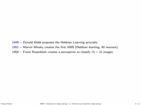
1949 – Donald Hebb proposes the Hebbian Learning principle.

1951 – Marvin Minsky creates the first ANN (Hebbian learning, 40 neurons).

1958 – Frank Rosenblatt creates a perceptron to classify 20 × 20 images.

1959 – David H. Hubel and Torsten Wiesel demonstrate orientation selectivity andcolumnar organization in the cat’s visual cortex.

1982 – Paul Werbos proposes back-propagation for ANNs.

Francois Fleuret AMMI – Introduction to Deep Learning / 1.1. Artificial neural networks to deep learning 9 / 21

Neocognitron

195

visuo[ oreo 9l< QSsOCiQtion o r e o - -

lower-order --,. higher-order .-,. ~ .grandmother retino - - , - L G B --,. simple ~ complex --,. hypercomplex hypercomplex " - - cell '~

F- 3 I-- . . . . l r I I I I 11

Uo ', ~' Usl -----> Ucl t~-~i Us2~ Uc2 ~ Us3----* Uc3 T [ I L ~ L J

Fig. 1. Correspondence between the hierarchy model by Hubel and Wiesel, and the neural network of the neocognitron

shifted in parallel from cell to cell. Hence, all the cells in a single cell-plane have receptive fields of the same function, but at different positions.

We will use notations Us~(k~,n ) to represent the output of an S-cell in the kr th S-plane in the l-th module, and Ucl(k~, n) to represent the output of a C-cell in the kr th C-plane in that module, where n is the two- dimensional co-ordinates representing the position of these cell's receptive fields in the input layer.

Figure 2 is a schematic diagram illustrating the interconnections between layers. Each tetragon drawn with heavy lines represents an S-plane or a C-plane, and each vertical tetragon drawn with thin lines, in which S-planes or C-planes are enclosed, represents an S-layer or a C-layer.

In Fig. 2, a cell of each layer receives afferent connections from the cells within the area enclosed by the elipse in its preceding layer. To be exact, as for the S-cells, the elipses in Fig. 2 does not show the connect- ing area but the connectable area to the S-cells. That is, all the interconnections coming from the elipses are not always formed, because the synaptic connections incoming to the S-cells have plasticity.

In Fig. 2, for the sake of simplicity of the figure, only one cell is shown in each cell-plane. In fact, all the cells in a cell-plane have input synapses of the same spatial distribution as shown in Fig. 3, and only the positions of the presynaptic cells are shifted in parallel from cell to cell.

R3 ~I

modifioble synapses

) unmodifiable synopses

Since the cells in the network are interconnected in a cascade as shown in Fig. 2, the deeper the layer is, the larger becomes the receptive field of each cell of that layer. The density of the cells in each cell-plane is so determined as to decrease in accordance with the increase of the size of the receptive fields. Hence, the total number of the cells in each cell-plane decreases with the depth of the cell-plane in the network. In the last module, the receptive field of each C-cell becomes so large as to cover the whole area of input layer U0, and each C-plane is so determined as to have only one C-cell.

The S-cells and C-cells are excitatory cells. That is, all the efferent synapses from these cells are excitatory. Although it is not shown in Fig. 2, we also have

Fig. 3. Illustration showing the input interconnections to the cells within a single cell-plane

Fig. 2. Schematic diagram illustrating the interconnections between layers in the neocognitron

Follows Hubel and Wiesel’s results.

(Fukushima, 1980)

Francois Fleuret AMMI – Introduction to Deep Learning / 1.1. Artificial neural networks to deep learning 10 / 21

Network for the T-C problem

Trained with back-prop.

(Rumelhart et al., 1988)

Francois Fleuret AMMI – Introduction to Deep Learning / 1.1. Artificial neural networks to deep learning 11 / 21

LeNet-5

����������� ����������������������������������� �"! �

INPUT 32x32

Convolutions SubsamplingConvolutions

C1: feature maps 6@28x28

Subsampling

S2: f. maps6@14x14

S4: f. maps 16@5x5

C5: layer120

C3: f. maps 16@10x10

F6: layer 84

Full connectionFull connection

Gaussian connections

OUTPUT 10

��:LH%k%�#k¨Vb31A1*%: 01+@Ar06.%31+�2/}!PZ+�h;+r06K��#To,��w24CUMU24_L.#01:L24C%,/_!hX+@.%31,/_�hX+r0G8f2436g�T#*%+@31+b}�243fD%:LH4: 065�31+@A@24H4C%: 01:L24C�k lv,/AO*�>#_�,/C%+Y:L5�,§}�+B,R01.#31+�F�,/>ZT�:�k +4k%,§51+r0�2/}�.%C%: 0658X*#2451+Y8f+@:LH4*U015b,/31+YA@24C%5 0131,/:LC%+@D�012�Q�+�:LD#+BCU06:LA�,/_�k

å�ê©è"ç�ï1ëíï�å�è"ÿ�ä ï¾î�å�æ�ê�ø�éÆè ç�ï1æ�ä"ï�úiø�ì�ÿ�ê û�å%�aï�ädð&ã�ç�ï�è"ä�å�ø�é�å��û�ï��ì�ï,*¹��ø�ï�éiè�å�é�ù��ø�å�ê ��ì�éiè"ä ì�ûkè ç�ï�ïUÄ�ï���è©ì�ë¹è"ç�ï1ê"ø��î¼ì�ø�ùOé�ì�é!�û�ø�é�ïdå�ä ø³è@�að��}ëkè ç�ï���ì�ï,*¹��ø�ï�éiè ø�êpê�î�å�û�û1��è"ç�ï�é5è"ç�ï©ÿ�é�ø�è�ì�æNï�ä�åè ï�êø�é5å¹�iÿ�åaê�ø��}û�ø�é�ï�å�ä�î\ì�ù�ï���å�é�ù1è ç�ï©ê"ÿ�!�«ê"å�î\æ�û�ø�é���û�å%��ï�ä�î¼ï�ä ï�û��û�ÿ�ä�ê¼è"ç�ïOø�é�æ�ÿ�è�ð �}ë¸è ç�ï¤��ì�ï,*¹��ø�ï�éiè1ø�ê¾û�å�ä��aï��wê"ÿ�!�«ê å�î¼æ�û�ø�é��ÿ�é�ø�è ê{��å�é��ï�ê"ï�ï�é&å�êYæNï�ä"ëíì�ä î¼ø�é��¾å ��é�ìaø�ê��:ý�� ¼ìaä�åL��é�ìaø�ê����ñ{"� ¸ëíÿ�é��£è ø�ìaé¼ù�ï�æNï�é�ù�ø�é��®ì�éSè"ç�ïYúrå�û�ÿ�ï¹ì�ë�è ç�ï��ø�åaê�ðgþ�ÿ�����ïdê@�ê"ø�úaïSû�å%��ï�ä êpì�ë���ì�é�úaì�û�ÿ�è"ø�ì�é�ê¸å�é�ù�ê"ÿ�!�«ê"å�î¼æ�û�ø�é��5å�ä ï�è@��æ�ø���å�û�û�å�û�è"ï�ä"é�åè"ïdùf��ä ï�ê"ÿ�û�è"ø�é��¾ø�éOå����øª�}æ���ä å�î\ø�ù B+wåèpï�å���ç&û�å%��ï�ä���è"ç�ïé�ÿ�î�Nï�ä¸ì�ëgëíïdåè ÿ�ä"ïSî�å�æ�ê�ø�êpø�é ��ä ï�å�ê"ï�ù&åaê è ç�ïSê"æ�å�è"ø�å�ûUä"ïdê�ìaû�ÿ!�è"ø�ì�é\ø�êUù�ï���ä ï�åaê�ïdù�ð (wå���ç©ÿ�é�ø³ègø�é�è ç�ï¹è"ç�ø�ä�ù�ç�ø�ù�ù�ï�éSû�å%��ï�äBø�é�©��?�ÿ�ä ï��¹î�å%��ç�årúaïgø�é�æ�ÿ�èb��ì�é�é�ï��£è ø�ìaé�ê�ëíä ì�î ê�ï�ú�ï�ä å�ûrëíï�åè ÿ�ä ï�î�å�æ�êø�é�è ç�ï æ�ä ï�ú�ø�ì�ÿ�ê�û�å%��ï�ä�ðkã�ç�ï���ìaé�ú�ì�û�ÿ�è ø�ìaé��ê"ÿ�!�«ê"å�î¼æ�û�ø�é��À��ì�îÀ��ø�é�åè ø�ìaé���ø�é�ê�æ�ø�ä ï�ù���&õ ÿ��ï�û�å�é�ù � ø�ïdê�ï�û< ê�é�ì�è"ø�ì�é�ê�ì�ë �"ê"ø�îÀ�æ�û�ï� ®å�é�ù �R��ìaî\æ�û�ï�£� ���ï�û�û�ê���ó¹åaêkø�î¼æ�û�ï�î¼ï�éaè ï�ù\ø�éÀ��ÿ�ô�ÿ�ê�ç�ø�î�å=< êñ ï�ì!��ì��aé�ø�è"ä ì�é � b ��O��è"ç�ìaÿ���ç&é�ì¥��û�ì��å�û�û�5ê�ÿ�æNï�ä ú�ø�ê"ï�ù5û�ï�å�ä"é�ø�é��æ�ä ì!��ï�ù�ÿ�ä"ï ê"ÿ���ç5å�ê��å���ôZ�}æ�ä ì�æ�å��aåè ø�ìaé�ó¹åaêYårúå�ø�û�å��û�ïpè"ç�ï�é�ð��û�å�äR��ï�ù�ï���ä ï�ï©ì�ë^ø�éiúå�ä"ø�å�é���ï è"ì¥��ï�ì�î¼ï�è ä"ø��®è"ä�å�é�ê{ëíìaä"î�åè ø�ìaé�êYì�ëè"ç�ï\ø�é�æ�ÿ�è ��å�é¦�ï�å���ç�ø�ï�ú�ï�ù·óYø³è çOè ç�ø�ê®æ�ä"ì���ä ï�ê ê�ø�ú�ï©ä ï�ù�ÿ��£è ø�ìaéì�ë�ê"æ�åè ø�å�û�ä ï�ê"ì�û�ÿ�è"ø�ì�é¹��ìaî¼æ�ï�é�ê"å�è"ïdù¨Z�\å æ�ä ì��aä"ïdê"ê"ø�úaï^ø�é���ä ï�åaê�ïì�ëNè"ç�ï ä"ø���ç�é�ïdê"êUì�ë�è ç�ï ä ï�æ�ä ï�ê"ï�éiè å�è"ø�ì�é�Á»è"ç�ï é�ÿ�î�Nï�ä�ì�ë�ëíïdåè ÿ�ä"ïî�å�æ�ê/£ðþ�ø�é ��ï å�û�û�è ç�ï®ówï�ø��açiè ê¹å�ä ï�û�ï�å�ä é�ïdù¾óYø�è"ç��å���ôZ�}æ�ä"ìaæ�å?�iåè ø�ìaé����ìaé�ú�ì�û�ÿ�è ø�ìaé�å�û�é�ï�è{ówìaä"ô�ê¨��å�é�Nï·ê�ï�ï�éÄå�ê�ê���éaè ç�ï�ê"ø¾�ø�é��Oè ç�ï�ø�äìóYé ëíï�å�è"ÿ�ä ï�ïU£�è"ä�å���è"ìaä�ð¾ã�ç�ï1ówï�ø��açaè©ê"ç�å�ä ø�é��:è"ï���ç�é�ø�iÿ�ï1ç�å�êè"ç�ï�ø�éiè"ï�ä ï�ê�è"ø�é�� ê�ø�ù�ï:ïUÄ�ï��£è¼ì�ë ä ï�ù�ÿ���ø�é��·è ç�ï:éiÿ�î�Nï�ä¼ì�ëYëíä ï�ïæ�å�ä å�î\ï�è"ï�ä ê���è"ç�ï�ä"ï��� ä ï�ù�ÿ���ø�é�� è ç�ï ����å�æ�å���ø³è@�� Æì�ë©è"ç�ï î�åo���ç�ø�é�ï�å�é�ù¼ä"ïdù�ÿ���ø�é��®è ç�ï��iå�æ¨�ï�è{ówï�ï�é¼è ï�ê�è^ï�ä ä"ìaä�å�é�ù\è ä å�ø�é�ø�é��ï�ä ä ì�ä � b&c'}ð¾ã�ç�ï�é�ï�è{ówìaä"ô·ø�é�©���ÿ�ä"ï`�&��ìaéiè å�ø�é�ê4b&c���� ;6��5 ��ì�é!�é�ï#�£è"ø�ì�é�ê��o�ÿ�èkìaé�û� ����� �6����è"ä�å�ø�é�å?�û�ï^ëíä"ï�ï^æ�å�ä å�î\ï�è"ï�ä êX�ï#��å�ÿ�ê�ïì�ëUè"ç�ï ówï�ø��açaè ê"ç�å�ä ø�é���ð�Bø�£�ï�ù��«ê"ø�¾�ï\�wìaéiúaì�û�ÿ�è"ø�ì�é�å�ûSñ�ï�è{ó¹ì�ä ô�êOç�årúaïÃNï�ï�éÂå�æ�æ�û�ø�ï�ùè"ì î�å�éZ�Kå�æ�æ�û�ø���åè ø�ìaé�ê��¹å�î\ìaé�� ì�è"ç�ï�ä¾ç�å�é�ù�óYä ø³è ø�é�� ä ï���ì��aé�øª�è"ø�ì�é$� b ��O� � b�� O��î�å���ç�ø�é�ïU�}æ�ä ø�éiè ï�ù ��ç�å�ä�å��£è ï�äpä"ï#��ì��aé�ø�è"ø�ì�é � b ��1�ì�é��mû�ø�é�ï9ç�å�é�ù�óYä ø³è ø�é��Âä ï���ì���é�ø³è ø�ìaé � b�5 O�·å�é�ù/ë�å���ï9ä ï���ì��aé�øª�è"ø�ì�é � b�; }ð �Bø�£�ï�ù��«ê"ø�¾�ïÃ��ìaéiúaì�û�ÿ�è"ø�ì�é�å�û©é�ï�è{ówìaä"ô�ê:è ç�åèÆê�ç�å�ä"ïó¹ï�ø��çiè ê¼å�û�ì�é�� å ê�ø�é��aû�ï:è"ï�î¼æ�ìaä å�û�ù�ø�î¼ï�é�ê�ø�ì�éÄå�ä ï�ô�é�ìóYé å�êã�ø�î\ï��O"pï�û�å%�pñ�ï�ÿ�ä�å�ûiñ ï�è{ówìaä"ô�ê�Á�ã$"¸ñ�ñpêRÂ�ðUã$"¸ñ�ñpê;ç�årú�ï�Nï�ï�éÿ�ê"ï�ùOø�é·æ�ç�ì�é�ï�î¼ïSä ï���ì���é�ø³è ø�ìaé�ÁíóYø�è"ç�ìaÿ�è®ê"ÿ�!�«ê å�î¼æ�û�ø�é���Â�� c��'1�

� c�¿O�¼ê�æNì�ôaï�éòó¹ì�ä�ù ä ï���ì���é�ø�è"ø�ì�é Á�óYø³è ç(ê"ÿ�!�«ê å�î¼æ�û�ø�é��� � c0� 1�� c b O� ì�é��mû�ø�é�ï ä"ï#��ì��aé�ø�è"ø�ì�é ì�ë¼ø�ê"ì�û�åè ï�ùWç�å�é�ù�óYä ø³è"è"ï�éy��ç�å�ä�å��4�è"ï�ä ê4� c&c&1��å�é�ù5ê�ø��é�åè"ÿ�ä"ï¸ú�ï�ä"ø�© ��å�è"ø�ì�é � c!��}ð

' �E� ¸�º�¸U»Z(��ã�ç�ø�ê�ê�ï#�£è"ø�ì�é&ù�ïdê���ä"øNï�êYø�é5î\ìaä"ï ù�ï�è å�ø�û;è"ç�ï©å�äR��ç�ø�è"ï#�£è ÿ�ä"ï®ì�ë

��ïdñ ï�èB� �!�Yè ç�ïx�wìaé�ú�ì�û�ÿ�è ø�ìaé�å�û¸ñ ï�ÿ�ä å�ûpñ ï�è{ówìaä"ôÄÿ�ê"ï�ù6ø�é-è"ç�ïïU£�æNï�ä ø�î¼ï�éaè�ê�ð �;ï�ñ ï�èB� ����ì�î¼æ�ä ø�ê"ï�ê �©û�å%�aï�ä�ê��ié�ì�è$��ìaÿ�éiè"ø�é��Sè"ç�ïø�é�æ�ÿ�è#��å�û�û�ì�ë;óYç�ø���ç¥��ì�éiè å�ø�é1è"ä�å�ø�é�å?�û�ï¸æ�å�ä�å�î¼ï�è"ï�ä�ê'Á�ówï�ø��açiè ê/£ðã�ç�ï�ø�é�æ�ÿ�è;ø�ê;åSb �%£ b0�^æ�øª£�ï�û�ø�î�å?�aï�ð;ã�ç�ø�ê;ø�ê�ê"ø��é�ø�© ��å�éiè"û��û�å�äR��ï�äè"ç�å�é5è"ç�ï©û�å�ä��aï�ê�è'��ç�å�ä�å���è"ï�äYø�é5è ç�ï�ù�å�è å?�å�ê"ï¢Á�åèpî\ìiê{è��A�o£��6�æ�ø�£�ï�û�ê���ï�éaè ï�ä ï�ù�ø�é åC�65o£��A5 ©�ï�û�ù�Â�ð1ã�ç�ï�ä ï�å�ê"ì�é ø�ê®è"ç�å�è©ø³è©ø�êù�ïdê�ø�ä å��û�ï è"ç�å�èpæNì�è ï�éiè"ø�å�ûkù�ø�ê{è ø�é���è"ø�ú�ï�ëíï�åè ÿ�ä ï�ê�ê"ÿ���ç·åaêpê�è"ä ì�ôaïï�é�ù��mæNì�ø�éiè ê¹ì�ä���ìaä"é�ï�ä���å�é1å�æ�æNï�å�äE�G²�»µ¯�¸ ?/¸�²�»r¸U¬gì�ë�è"ç�ïpä ï���ï�æ!�è"ø�ú�ï�©�ï�û�ù:ì�ë;è"ç�ï ç�ø��aç�ï�ê�èB�}û�ï�ú�ï�ûNëíï�åè ÿ�ä ï®ù�ï�è"ï#�£è ì�ä�ê�ðY�«éO��ïdñ ï�è����è"ç�ïpê"ï�èwì�ë���ï�éiè ï�ä�ê�ì�ë�è ç�ï�ä ï���ï�æ�è ø�úaï$©�ï�û�ù�êwì�ë�è ç�ï�û�å�ê�è���ì�é�ú�ìaû�ÿ!�è"ø�ì�é�å�û�û�å%��ï�ä�ÁO�;b���ê"ï�ï$Nï�û�ìó'Â;ëíì�ä îÂå4�A�?£��A�¸å�ä ï�åpø�é\è"ç�ï'��ï�éaè ï�äì�ë;è"ç�ï4b �o£ b �®ø�é�æ�ÿ�èdð^ã�ç�ï¸úå�û�ÿ�ï�ê¹ì�ëBè"ç�ï¸ø�é�æ�ÿ�è æ�ø�£�ï�û�ê�å�ä ï�é�ìaäB�î�å�û�ø�¾�ï�ù�ê�ì�è"ç�å�è®è"ç�ï¨�å���ôZ�aä"ìaÿ�é�ù&û�ï�úaï�û$ÁíóYç�ø³è ï#Ât��ìaä"ä ï�ê"æNì�é�ù�êè"ì&å:úå�û�ÿ�ï¼ì�ë�� ��ð�¿\å�é�ùOè"ç�ï¼ëíìaä"ï���ä ì�ÿ�é�ù�Áµ�û�å���ô�Â���ìaä"ä ï�ê"æNì�é�ù�êè"ìx¿að�¿��'��ð¼ã�ç�ø�ê î�å�ô�ï�ê¸è ç�ï�î¼ï�å�é ø�é�æ�ÿ�è�ä"ìaÿ���ç�û��!���Bå�é�ù�è"ç�ïúå�ä ø�å�é���ï¸ä ì�ÿ��aç�û�� ¿¸óYç�ø��ç5å�����ï�û�ï�ä�åè ï�ê¹û�ï�å�ä é�ø�é��O� c � }ð�«é®è"ç�ï^ëíì�û�û�ìóYø�é����%��ìaé�ú�ì�û�ÿ�è ø�ìaé�å�ûû�å%��ï�ä ê�å�ä"ïgû�å?Nï�û�ï�ù��§£f�ê"ÿ�!�ê å�î¼æ�û�ø�é���û�å%�aï�ä�ê�å�ä"ï©û�å?Nï�û�ï�ù þZ£f��å�é�ù·ëíÿ�û�û�Z�O��ì�é�é�ï��£è ï�ù&û�å%��ï�ä êå�ä ï®û�å��ï�û�ïdù¥�X£f��óYç�ï�ä"ï�£:ø�ê¹è ç�ï û�å%�aï�ä�ø�é�ù�ïU£�ð�;å%��ï�ä��{¿¾ø�ê�å���ìaé�ú�ì�û�ÿ�è ø�ìaé�å�ûgû�å%��ï�ä©óYø³è ç)�5ëíï�å�è"ÿ�ä ï�î�å�æ�ê�ð

(^å���ç¼ÿ�é�ø�è¹ø�é�ï�å���ç¼ëíï�åè ÿ�ä ï î�å�æ¾ø�ê§��ì�é�é�ï#�£è ï�ù¼è ì�å �%£��®é�ï�ø��ç!�Nì�ä ç�ì�ì�ù�ø�é�è"ç�ï�ø�é�æ�ÿ�èdðUã�ç�ï�ê"ø¾�ï^ì�ë�è ç�ï^ëíïdåè ÿ�ä"ï¹î�å�æ�êUø�ê �A5o£��65óYç�ø���çOæ�ä ï�úaï�éiè êt��ì�é�é�ï#�£è ø�ìaé·ëíä ì�î è"ç�ï\ø�é�æ�ÿ�è ëíä"ìaî ë�å�û�û�ø�é��:ì?Äè"ç�ï�Nì�ÿ�é�ù�å�äR��ð��{¿���ì�éiè å�ø�é�ê�¿ �6�¼è"ä�å�ø�é�å?�û�ïSæ�å�ä�å�î¼ï�è ï�ä�ê��Nå�é�ù¿ � �!� b6�&c���ìaé�é�ï#�£è"ø�ì�é�ê�ð�;å%��ï�ä þ �\ø�ê�å�ê�ÿ���}ê å�î¼æ�û�ø�é��\û�å%��ï�äYóYø³è ç �Sëíï�åè ÿ�ä ï î¼å�æ�êYì�ëê"ø�¾�ï�¿�c?£f¿]c�ð#(^å���ç�ÿ�é�ø³ègø�é\ïdå���ç�ëíï�åè ÿ�ä ï¹î�å�æSø�ê���ìaé�é�ï���è"ïdù©è ì¸å

�%£��®é�ï�ø��ç��ìaä"ç�ìiì�ù¼ø�é�è"ç�ï{��ìaä"ä ï�ê"æNì�é�ù�ø�é��®ëíïdåè"ÿ�ä"ïpî¼å�æ�ø�é&�{¿�ðã�ç�ï¸ëíì�ÿ�äYø�é�æ�ÿ�è ê�è ì�å�ÿ�é�ø³è ø�é·þ ��å�ä"ï åaù�ù�ï�ù���è"ç�ï�é�îSÿ�û³è ø�æ�û�ø�ï�ù�� å&è"ä�å�ø�é�å��û�ï���ì�ïC*¢��ø�ï�éaè#��å�é�ùKå�ù�ù�ï�ùÆè ì å·è"ä�å�ø�é�å?�û�ï¢�ø�å�ê�ðã�ç�ï·ä ï�ê"ÿ�û�è¾ø�ê1æ�å�ê ê"ï�ùKè"ç�ä ì�ÿ���çHå ê�ø��î¼ìaø�ù�å�û�ëíÿ�é���è"ø�ì�é�ð ã�ç�ï�%£��1ä"ï#��ï�æ�è"ø�ú�ï�©�ï�û�ù�ê å�ä"ïSé�ì�é!�}ìú�ï�ä"û�å�æ�æ�ø�é�����è"ç�ï�ä"ï�ëíì�ä ï�ëíïdåè"ÿ�ä"ïî�å�æ�ê�ø�éhþ��5ç�årú�ï¼ç�å�û³ë�è ç�ï1é�ÿ�î��ï�ä�ì�ë�ä ìó ê©å�é�ùx��ì�û�ÿ�î¼é å�êëíï�å�è"ÿ�ä ï®î�å�æ�êYø�é �{¿�ð �Bå%��ï�äYþ �\ç�åaêt¿ ��è"ä�å�ø�é�å��û�ï®æ�å�ä å�î¼ï�è"ï�ä êå�é�ù.��� 5�56�À��ì�é�é�ï���è"ø�ì�é�ê�ð�;å%��ï�ä��;b¼ø�êpå¢��ì�é�ú�ìaû�ÿ�è"ø�ì�é�å�û�û�å%�aï�ä óYø�è"ç�¿��\ëíï�å�è"ÿ�ä ï©î�å�æ�ê�ð

(^å���ç5ÿ�é�ø�è�ø�é&ïdå���ç:ëíï�å�è"ÿ�ä ï©î�å�æ5ø�ê'��ì�é�é�ï#�£è ï�ù�è"ì1ê"ï�úaï�ä�å�û �o£ �é�ï�ø��açZNì�ä ç�ì�ì�ù�ê5åè&ø�ù�ï�éiè"ø���å�û®û�ì!��å�è"ø�ì�é�ê5ø�é åKê"ÿ��ê"ï�è·ì�ë¼þ �=< êëíï�å�è"ÿ�ä ï:î¼å�æ�ê�ðKãUå?�û�ï¥�\ê�ç�ìó ê�è ç�ï&ê�ï�è\ì�ë®þ �·ëíï�å�è"ÿ�ä ï:î¼å�æ�ê

(leCun et al., 1998)

Francois Fleuret AMMI – Introduction to Deep Learning / 1.1. Artificial neural networks to deep learning 12 / 21

AlexNet

Figure 2: An illustration of the architecture of our CNN, explicitly showing the delineation of responsibilitiesbetween the two GPUs. One GPU runs the layer-parts at the top of the figure while the other runs the layer-partsat the bottom. The GPUs communicate only at certain layers. The network’s input is 150,528-dimensional, andthe number of neurons in the network’s remaining layers is given by 253,440–186,624–64,896–64,896–43,264–4096–4096–1000.

neurons in a kernel map). The second convolutional layer takes as input the (response-normalizedand pooled) output of the first convolutional layer and filters it with 256 kernels of size 5× 5× 48.The third, fourth, and fifth convolutional layers are connected to one another without any interveningpooling or normalization layers. The third convolutional layer has 384 kernels of size 3 × 3 ×256 connected to the (normalized, pooled) outputs of the second convolutional layer. The fourthconvolutional layer has 384 kernels of size 3 × 3 × 192 , and the fifth convolutional layer has 256kernels of size 3× 3× 192. The fully-connected layers have 4096 neurons each.

4 Reducing Overfitting

Our neural network architecture has 60 million parameters. Although the 1000 classes of ILSVRCmake each training example impose 10 bits of constraint on the mapping from image to label, thisturns out to be insufficient to learn so many parameters without considerable overfitting. Below, wedescribe the two primary ways in which we combat overfitting.

4.1 Data Augmentation

The easiest and most common method to reduce overfitting on image data is to artificially enlargethe dataset using label-preserving transformations (e.g., [25, 4, 5]). We employ two distinct formsof data augmentation, both of which allow transformed images to be produced from the originalimages with very little computation, so the transformed images do not need to be stored on disk.In our implementation, the transformed images are generated in Python code on the CPU while theGPU is training on the previous batch of images. So these data augmentation schemes are, in effect,computationally free.

The first form of data augmentation consists of generating image translations and horizontal reflec-tions. We do this by extracting random 224× 224 patches (and their horizontal reflections) from the256×256 images and training our network on these extracted patches4. This increases the size of ourtraining set by a factor of 2048, though the resulting training examples are, of course, highly inter-dependent. Without this scheme, our network suffers from substantial overfitting, which would haveforced us to use much smaller networks. At test time, the network makes a prediction by extractingfive 224 × 224 patches (the four corner patches and the center patch) as well as their horizontalreflections (hence ten patches in all), and averaging the predictions made by the network’s softmaxlayer on the ten patches.

The second form of data augmentation consists of altering the intensities of the RGB channels intraining images. Specifically, we perform PCA on the set of RGB pixel values throughout theImageNet training set. To each training image, we add multiples of the found principal components,

4This is the reason why the input images in Figure 2 are 224× 224× 3-dimensional.

5

(Krizhevsky et al., 2012)

Francois Fleuret AMMI – Introduction to Deep Learning / 1.1. Artificial neural networks to deep learning 13 / 21

GoogLeNet

input

Conv7x7+2(S)

MaxPool3x3+2(S)

LocalRespNorm

Conv1x1+1(V)

Conv3x3+1(S)

LocalRespNorm

MaxPool3x3+2(S)

Conv1x1+1(S)

Conv1x1+1(S)

Conv1x1+1(S)

MaxPool3x3+1(S)

DepthConcat

Conv3x3+1(S)

Conv5x5+1(S)

Conv1x1+1(S)

Conv1x1+1(S)

Conv1x1+1(S)

Conv1x1+1(S)

MaxPool3x3+1(S)

DepthConcat

Conv3x3+1(S)

Conv5x5+1(S)

Conv1x1+1(S)

MaxPool3x3+2(S)

Conv1x1+1(S)

Conv1x1+1(S)

Conv1x1+1(S)

MaxPool3x3+1(S)

DepthConcat

Conv3x3+1(S)

Conv5x5+1(S)

Conv1x1+1(S)

Conv1x1+1(S)

Conv1x1+1(S)

Conv1x1+1(S)

MaxPool3x3+1(S)

AveragePool5x5+3(V)

DepthConcat

Conv3x3+1(S)

Conv5x5+1(S)

Conv1x1+1(S)

Conv1x1+1(S)

Conv1x1+1(S)

Conv1x1+1(S)

MaxPool3x3+1(S)

DepthConcat

Conv3x3+1(S)

Conv5x5+1(S)

Conv1x1+1(S)

Conv1x1+1(S)

Conv1x1+1(S)

Conv1x1+1(S)

MaxPool3x3+1(S)

DepthConcat

Conv3x3+1(S)

Conv5x5+1(S)

Conv1x1+1(S)

Conv1x1+1(S)

Conv1x1+1(S)

Conv1x1+1(S)

MaxPool3x3+1(S)

AveragePool5x5+3(V)

DepthConcat

Conv3x3+1(S)

Conv5x5+1(S)

Conv1x1+1(S)

MaxPool3x3+2(S)

Conv1x1+1(S)

Conv1x1+1(S)

Conv1x1+1(S)

MaxPool3x3+1(S)

DepthConcat

Conv3x3+1(S)

Conv5x5+1(S)

Conv1x1+1(S)

Conv1x1+1(S)

Conv1x1+1(S)

Conv1x1+1(S)

MaxPool3x3+1(S)

DepthConcat

Conv3x3+1(S)

Conv5x5+1(S)

Conv1x1+1(S)

AveragePool7x7+1(V)

FC

Conv1x1+1(S)

FC

FC

SoftmaxActivation

softmax0

Conv1x1+1(S)

FC

FC

SoftmaxActivation

softmax1

SoftmaxActivation

softmax2

Figure 3: GoogLeNet network with all the bells and whistles

7

(Szegedy et al., 2015)

Francois Fleuret AMMI – Introduction to Deep Learning / 1.1. Artificial neural networks to deep learning 14 / 21

Resnet

7x7 conv, 64, /2

pool, /2

3x3 conv, 64

3x3 conv, 64

3x3 conv, 64

3x3 conv, 64

3x3 conv, 64

3x3 conv, 64

3x3 conv, 128, /2

3x3 conv, 128

3x3 conv, 128

3x3 conv, 128

3x3 conv, 128

3x3 conv, 128

3x3 conv, 128

3x3 conv, 128

3x3 conv, 256, /2

3x3 conv, 256

3x3 conv, 256

3x3 conv, 256

3x3 conv, 256

3x3 conv, 256

3x3 conv, 256

3x3 conv, 256

3x3 conv, 256

3x3 conv, 256

3x3 conv, 256

3x3 conv, 256

3x3 conv, 512, /2

3x3 conv, 512

3x3 conv, 512

3x3 conv, 512

3x3 conv, 512

3x3 conv, 512

avg pool

fc 1000

image

3x3 conv, 512

3x3 conv, 64

3x3 conv, 64

pool, /2

3x3 conv, 128

3x3 conv, 128

pool, /2

3x3 conv, 256

3x3 conv, 256

3x3 conv, 256

3x3 conv, 256

pool, /2

3x3 conv, 512

3x3 conv, 512

3x3 conv, 512

pool, /2

3x3 conv, 512

3x3 conv, 512

3x3 conv, 512

3x3 conv, 512

pool, /2

fc 4096

fc 4096

fc 1000

image

output

size: 112

output

size: 224

output

size: 56

output

size: 28

output

size: 14

output

size: 7

output

size: 1

VGG-19 34-layer plain

7x7 conv, 64, /2

pool, /2

3x3 conv, 64

3x3 conv, 64

3x3 conv, 64

3x3 conv, 64

3x3 conv, 64

3x3 conv, 64

3x3 conv, 128, /2

3x3 conv, 128

3x3 conv, 128

3x3 conv, 128

3x3 conv, 128

3x3 conv, 128

3x3 conv, 128

3x3 conv, 128

3x3 conv, 256, /2

3x3 conv, 256

3x3 conv, 256

3x3 conv, 256

3x3 conv, 256

3x3 conv, 256

3x3 conv, 256

3x3 conv, 256

3x3 conv, 256

3x3 conv, 256

3x3 conv, 256

3x3 conv, 256

3x3 conv, 512, /2

3x3 conv, 512

3x3 conv, 512

3x3 conv, 512

3x3 conv, 512

3x3 conv, 512

avg pool

fc 1000

image

34-layer residual

Figure 3. Example network architectures for ImageNet. Left: theVGG-19 model [41] (19.6 billion FLOPs) as a reference. Mid-dle: a plain network with 34 parameter layers (3.6 billion FLOPs).Right: a residual network with 34 parameter layers (3.6 billionFLOPs). The dotted shortcuts increase dimensions. Table 1 showsmore details and other variants.

Residual Network. Based on the above plain network, weinsert shortcut connections (Fig. 3, right) which turn thenetwork into its counterpart residual version. The identityshortcuts (Eqn.(1)) can be directly used when the input andoutput are of the same dimensions (solid line shortcuts inFig. 3). When the dimensions increase (dotted line shortcutsin Fig. 3), we consider two options: (A) The shortcut stillperforms identity mapping, with extra zero entries paddedfor increasing dimensions. This option introduces no extraparameter; (B) The projection shortcut in Eqn.(2) is used tomatch dimensions (done by 1×1 convolutions). For bothoptions, when the shortcuts go across feature maps of twosizes, they are performed with a stride of 2.

3.4. Implementation

Our implementation for ImageNet follows the practicein [21, 41]. The image is resized with its shorter side ran-domly sampled in [256, 480] for scale augmentation [41].A 224×224 crop is randomly sampled from an image or itshorizontal flip, with the per-pixel mean subtracted [21]. Thestandard color augmentation in [21] is used. We adopt batchnormalization (BN) [16] right after each convolution andbefore activation, following [16]. We initialize the weightsas in [13] and train all plain/residual nets from scratch. Weuse SGD with a mini-batch size of 256. The learning ratestarts from 0.1 and is divided by 10 when the error plateaus,and the models are trained for up to 60× 104 iterations. Weuse a weight decay of 0.0001 and a momentum of 0.9. Wedo not use dropout [14], following the practice in [16].

In testing, for comparison studies we adopt the standard10-crop testing [21]. For best results, we adopt the fully-convolutional form as in [41, 13], and average the scoresat multiple scales (images are resized such that the shorterside is in {224, 256, 384, 480, 640}).

4. Experiments4.1. ImageNet Classification

We evaluate our method on the ImageNet 2012 classifi-cation dataset [36] that consists of 1000 classes. The modelsare trained on the 1.28 million training images, and evalu-ated on the 50k validation images. We also obtain a finalresult on the 100k test images, reported by the test server.We evaluate both top-1 and top-5 error rates.

Plain Networks. We first evaluate 18-layer and 34-layerplain nets. The 34-layer plain net is in Fig. 3 (middle). The18-layer plain net is of a similar form. See Table 1 for de-tailed architectures.

The results in Table 2 show that the deeper 34-layer plainnet has higher validation error than the shallower 18-layerplain net. To reveal the reasons, in Fig. 4 (left) we com-pare their training/validation errors during the training pro-cedure. We have observed the degradation problem - the

4

(He et al., 2015)

Francois Fleuret AMMI – Introduction to Deep Learning / 1.1. Artificial neural networks to deep learning 15 / 21

Deep learning is built on a natural generalization of a neural network: a graphof tensor operators, taking advantage of

• the chain rule (aka “back-propagation”),

• stochastic gradient decent,

• convolutions,

• parallel operations on GPUs.

This does not differ much from networks from the 90s

Francois Fleuret AMMI – Introduction to Deep Learning / 1.1. Artificial neural networks to deep learning 16 / 21

This generalization allows to design complex networks of operators dealing withimages, sound, text, sequences, etc. and to train them end-to-end.

(Yeung et al., 2015)

Francois Fleuret AMMI – Introduction to Deep Learning / 1.1. Artificial neural networks to deep learning 17 / 21

CIFAR10

32 × 32 color images, 50k train samples, 10k test samples.

(Krizhevsky, 2009, chap. 3)

Francois Fleuret AMMI – Introduction to Deep Learning / 1.1. Artificial neural networks to deep learning 18 / 21

Performance on CIFAR10

75

80

85

90

95

100

2010 2012 2014 2016 2018

Krizhevsky et al. (2012)

Graham (2015)

Human performance

Real et al. (2018)

Acc

ura

cy (

%)

Year

Francois Fleuret AMMI – Introduction to Deep Learning / 1.1. Artificial neural networks to deep learning 19 / 21

ImageNet Large Scale Visual Recognition Challenge.

1000 categories, > 1M images

(http://image-net.org/challenges/LSVRC/2014/browse-synsets)

Francois Fleuret AMMI – Introduction to Deep Learning / 1.1. Artificial neural networks to deep learning 20 / 21

ImageNet Large Scale Visual Recognition Challenge.

1000 categories, > 1M images

(http://image-net.org/challenges/LSVRC/2014/browse-synsets)

Francois Fleuret AMMI – Introduction to Deep Learning / 1.1. Artificial neural networks to deep learning 20 / 21

ImageNet Large Scale Visual Recognition Challenge.

1000 categories, > 1M images

(http://image-net.org/challenges/LSVRC/2014/browse-synsets)

Francois Fleuret AMMI – Introduction to Deep Learning / 1.1. Artificial neural networks to deep learning 20 / 21

model top-1 err. top-5 err.

VGG-16 [41] 28.07 9.33GoogLeNet [44] - 9.15PReLU-net [13] 24.27 7.38

plain-34 28.54 10.02ResNet-34 A 25.03 7.76ResNet-34 B 24.52 7.46ResNet-34 C 24.19 7.40ResNet-50 22.85 6.71ResNet-101 21.75 6.05ResNet-152 21.43 5.71

Table 3. Error rates (%, 10-crop testing) on ImageNet validation.VGG-16 is based on our test. ResNet-50/101/152 are of option Bthat only uses projections for increasing dimensions.

method top-1 err. top-5 err.

VGG [41] (ILSVRC’14) - 8.43†

GoogLeNet [44] (ILSVRC’14) - 7.89VGG [41] (v5) 24.4 7.1PReLU-net [13] 21.59 5.71BN-inception [16] 21.99 5.81ResNet-34 B 21.84 5.71ResNet-34 C 21.53 5.60ResNet-50 20.74 5.25ResNet-101 19.87 4.60ResNet-152 19.38 4.49

Table 4. Error rates (%) of single-model results on the ImageNetvalidation set (except † reported on the test set).

method top-5 err. (test)VGG [41] (ILSVRC’14) 7.32GoogLeNet [44] (ILSVRC’14) 6.66VGG [41] (v5) 6.8PReLU-net [13] 4.94BN-inception [16] 4.82ResNet (ILSVRC’15) 3.57

Table 5. Error rates (%) of ensembles. The top-5 error is on thetest set of ImageNet and reported by the test server.

ResNet reduces the top-1 error by 3.5% (Table 2), resultingfrom the successfully reduced training error (Fig. 4 right vs.left). This comparison verifies the effectiveness of residuallearning on extremely deep systems.

Last, we also note that the 18-layer plain/residual netsare comparably accurate (Table 2), but the 18-layer ResNetconverges faster (Fig. 4 right vs. left). When the net is “notoverly deep” (18 layers here), the current SGD solver is stillable to find good solutions to the plain net. In this case, theResNet eases the optimization by providing faster conver-gence at the early stage.

Identity vs. Projection Shortcuts. We have shown that

3x3, 64

1x1, 64

relu

1x1, 256

relu

relu

3x3, 64

3x3, 64

relu

relu

64-d 256-d

Figure 5. A deeper residual function F for ImageNet. Left: abuilding block (on 56×56 feature maps) as in Fig. 3 for ResNet-34. Right: a “bottleneck” building block for ResNet-50/101/152.

parameter-free, identity shortcuts help with training. Nextwe investigate projection shortcuts (Eqn.(2)). In Table 3 wecompare three options: (A) zero-padding shortcuts are usedfor increasing dimensions, and all shortcuts are parameter-free (the same as Table 2 and Fig. 4 right); (B) projec-tion shortcuts are used for increasing dimensions, and othershortcuts are identity; and (C) all shortcuts are projections.

Table 3 shows that all three options are considerably bet-ter than the plain counterpart. B is slightly better than A. Weargue that this is because the zero-padded dimensions in Aindeed have no residual learning. C is marginally better thanB, and we attribute this to the extra parameters introducedby many (thirteen) projection shortcuts. But the small dif-ferences among A/B/C indicate that projection shortcuts arenot essential for addressing the degradation problem. So wedo not use option C in the rest of this paper, to reduce mem-ory/time complexity and model sizes. Identity shortcuts areparticularly important for not increasing the complexity ofthe bottleneck architectures that are introduced below.

Deeper Bottleneck Architectures. Next we describe ourdeeper nets for ImageNet. Because of concerns on the train-ing time that we can afford, we modify the building blockas a bottleneck design4. For each residual function F , weuse a stack of 3 layers instead of 2 (Fig. 5). The three layersare 1×1, 3×3, and 1×1 convolutions, where the 1×1 layersare responsible for reducing and then increasing (restoring)dimensions, leaving the 3×3 layer a bottleneck with smallerinput/output dimensions. Fig. 5 shows an example, whereboth designs have similar time complexity.

The parameter-free identity shortcuts are particularly im-portant for the bottleneck architectures. If the identity short-cut in Fig. 5 (right) is replaced with projection, one canshow that the time complexity and model size are doubled,as the shortcut is connected to the two high-dimensionalends. So identity shortcuts lead to more efficient modelsfor the bottleneck designs.

50-layer ResNet: We replace each 2-layer block in the

4Deeper non-bottleneck ResNets (e.g., Fig. 5 left) also gain accuracyfrom increased depth (as shown on CIFAR-10), but are not as economicalas the bottleneck ResNets. So the usage of bottleneck designs is mainly dueto practical considerations. We further note that the degradation problemof plain nets is also witnessed for the bottleneck designs.

6

(He et al., 2015)

Francois Fleuret AMMI – Introduction to Deep Learning / 1.1. Artificial neural networks to deep learning 21 / 21

The end

References

K. Fukushima. Neocognitron: A self-organizing neural network model for a mechanism ofpattern recognition unaffected by shift in position. Biological Cybernetics, 36(4):193–202, April 1980.

K. He, X. Zhang, S. Ren, and J. Sun. Deep residual learning for image recognition. CoRR,abs/1512.03385, 2015.

A. Krizhevsky. Learning multiple layers of features from tiny images. Master’s thesis,Department of Computer Science, University of Toronto, 2009.

A. Krizhevsky, I. Sutskever, and G. Hinton. Imagenet classification with deep convolutionalneural networks. In Neural Information Processing Systems (NIPS), 2012.

Y. leCun, L. Bottou, Y. Bengio, and P. Haffner. Gradient-based learning applied todocument recognition. Proceedings of the IEEE, 86(11):2278–2324, 1998.

W. S. McCulloch and W. Pitts. A logical calculus of the ideas immanent in nervous activity.The bulletin of mathematical biophysics, 5(4):115–133, 1943.

D. E. Rumelhart, G. E. Hinton, and R. J. Williams. Neurocomputing: Foundations ofResearch, chapter Learning Representations by Back-propagating Errors, pages 696–699.MIT Press, 1988.

C. Szegedy, W. Liu, Y. Jia, P. Sermanet, S. Reed, D. Anguelov, D. Erhan, V. Vanhoucke,and A. Rabinovich. Going deeper with convolutions. In Conference on Computer Visionand Pattern Recognition (CVPR), 2015.

S. Yeung, O. Russakovsky, G. Mori, and L. Fei-Fei. End-to-end learning of action detectionfrom frame glimpses in videos. CoRR, abs/1511.06984, 2015.