An Abstract Domain of Uninterpreted Functions

Graeme Gange1, Jorge A. Navas2, Peter Schachte1, Harald Søndergaard1, andPeter J. Stuckey1

1 Department of Computing and Information Systems,The University of Melbourne, Victoria 3010, Australia{gkgange,schachte,harald,pstuckey}@unimelb.edu.au

2 NASA Ames Research Center, Moffett Field, CA 94035, USAjorge.a.navaslaserna@nasa.gov

Abstract. We revisit relational static analysis of numeric variables.Such analyses face two difficulties. First, even inexpensive relational do-mains scale too poorly to be practical for large code-bases. Second, toremain tractable they have extremely coarse handling of non-linear re-lations. In this paper, we introduce the subterm domain, a weakly rela-tional abstract domain for inferring equivalences amongst sub-expressions,based on the theory of uninterpreted functions. This provides an ex-tremely cheap approach for enriching non-relational domains with rela-tional information, and enhances precision of both relational and non-relational domains in the presence of non-linear operations. We evaluatethe idea in the context of the software verification tool SeaHorn.

1 Introduction

This paper investigates a new approach to relational analysis. Our aim is todevelop a method that scales to very large code bases, yet maintains a reasonabledegree of precision, also for programs that use non-linear numeric operations.

Abstract interpretation is a well-established theoretical framework for soundreasoning about program properties. It provides means for comparing programanalyses, especially with respect to the granularity of information (precision)that analyses allow us to statically extract from programs. On the whole, reduc-ing such questions to questions about abstract domains. An abstract domain,essentially, specifies the (limited) language of judgements we are able to usewhen reasoning statically about a program’s runtime behaviour.

A class of abstract domains that has received particular attention are thenumeric domains—those supporting reasoning about variables of numeric (of-ten integer or rational) type. Numeric domains are important because of thenumerous applications in termination and safety analyses, such as overflow de-tection and out-of-bounds array analysis. The polyhedral abstract domain [9]allows us to express linear arithmetic constraints (equalities and inequalities)over program state spaces of arbitrary finite dimension k. But high expressive-ness comes at a cost; analysis using the polyhedral domain does not scale wellto large code bases. For this reason, a number of abstract domains have beenproposed, seeking to strike a better balance between cost and expressiveness.

Language restriction. The primary way of doing this is to limit expressive-ness, that is, to restrict the language of allowed judgements. Most commonlythis is done by expressing only 1- or 2-dimensional projections of the program’s(abstract) state space, often banning all but a limited set of coefficients in linearconstraints. Examples of this kind of restriction to polyhedral analysis abound,including zones [19], TVPI [23, 22], octagons [20], pentagons [18], and logahe-dra [14]. These avoid the exponential behaviour of polyhedra, instead offeringpolynomial (typically quadratic or cubic) decision and normalization procedures.Still, they have been observed to be too expensive in practice for industrial code-bases [18, 24]. Hence other “restrictive” techniques have been proposed which aresometimes integral to an analysis, sometimes orthogonal.

Dimensionality restriction. These methods aim to lower the dimension kof the program (abstract) state space, by replacing the full space with severallower-dimension subspaces. Variables are separated into “buckets” or packs ac-cording to some criterion. Usually the packs are disjoint, and relations can beexplored only amongst variables in the same pack (relaxations of this have alsobeen proposed [4]). The criterion for pack membership may be syntactic [8] ordetermined dynamically [24]. A variant is to only permit relations between sets;in the Gauge domain [25], relations are only maintained between program vari-ables and introduced loop counters, not between sets of program variables.

Closure restriction. Some methods abandon the systematic transitive closureof relations (and therefore lack a normal form for constraints). Constraints thatfollow by transitive closure may be discovered lazily, or not at all. Closure re-striction was used successfully with the pentagon domain; a tolerable loss ofprecision was compensated for by a significant cost reduction [18].

All of the work discussed up to this point has, in some sense, started from an ideal(polyhedral) analysis and applied restrictions to the degree of “relationality.” Adifferent line of work starts from very basic analyses and adds mechanisms tocapture relational information. These approaches do not focus on restrictions,but rather on how to compensate for limited precision using “symbolic” reason-ing. Such symbolic methods maintain selected syntactic information about com-putations and use this to enhance precision. The primary examples are Mine’slinearization method [21], based on “symbolic constant propagation” and Changand Leino’s congruence closure extension [5].

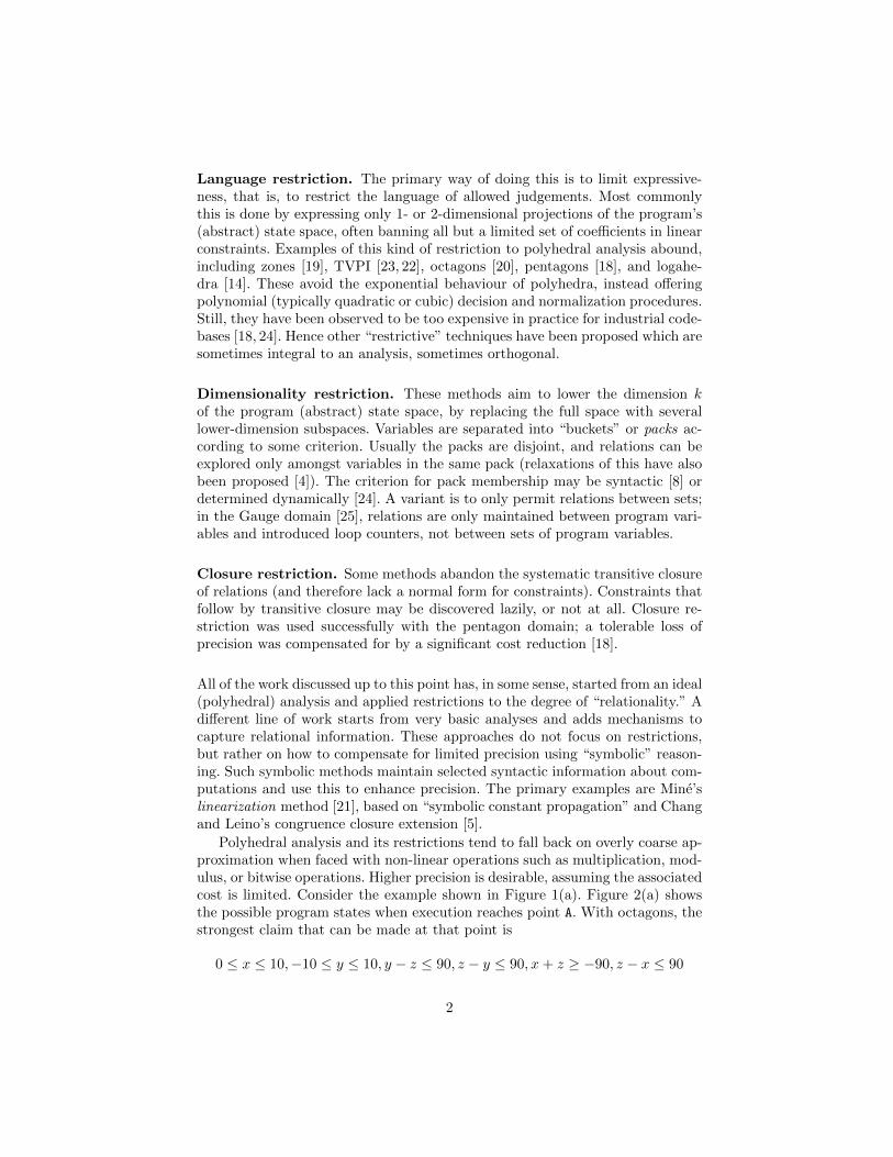
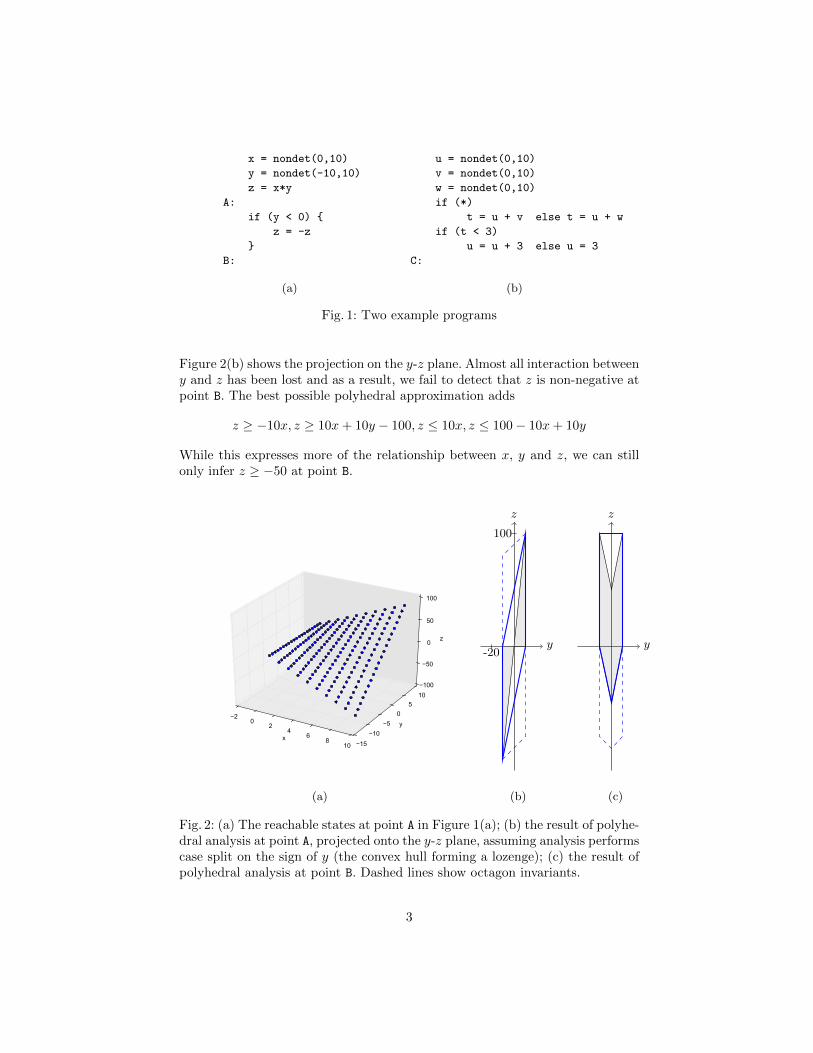
Polyhedral analysis and its restrictions tend to fall back on overly coarse ap-proximation when faced with non-linear operations such as multiplication, mod-ulus, or bitwise operations. Higher precision is desirable, assuming the associatedcost is limited. Consider the example shown in Figure 1(a). Figure 2(a) showsthe possible program states when execution reaches point A. With octagons, thestrongest claim that can be made at that point is

0 ≤ x ≤ 10,−10 ≤ y ≤ 10, y − z ≤ 90, z − y ≤ 90, x+ z ≥ −90, z − x ≤ 90

2

x = nondet(0,10)

y = nondet(-10,10)

z = x*y

A:

if (y < 0) {

z = -z

}

B:

(a)

u = nondet(0,10)

v = nondet(0,10)

w = nondet(0,10)

if (*)

t = u + v else t = u + w

if (t < 3)

u = u + 3 else u = 3

C:

(b)

Fig. 1: Two example programs

Figure 2(b) shows the projection on the y-z plane. Almost all interaction betweeny and z has been lost and as a result, we fail to detect that z is non-negative atpoint B. The best possible polyhedral approximation adds

z ≥ −10x, z ≥ 10x+ 10y − 100, z ≤ 10x, z ≤ 100− 10x+ 10y

While this expresses more of the relationship between x, y and z, we can stillonly infer z ≥ −50 at point B.

x

−20

24

68

10

y

−15−10

−50

510

z

−100

−50

0

50

100

y

z

100

-20y

z

(a) (b) (c)

Fig. 2: (a) The reachable states at point A in Figure 1(a); (b) the result of polyhe-dral analysis at point A, projected onto the y-z plane, assuming analysis performscase split on the sign of y (the convex hull forming a lozenge); (c) the result ofpolyhedral analysis at point B. Dashed lines show octagon invariants.

3

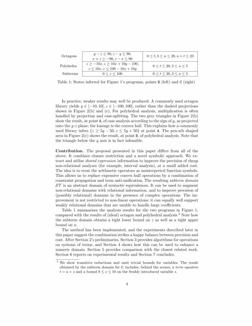
Octagonsy − z ≤ 90, z − y ≤ 90,

0 ≤ t, 3 ≤ u ≤ 20, u+ t ≤ 23x+ z ≥ −90, z − x ≤ 90

Polyhedraz ≥ −10x, z ≥ 10x+ 10y − 100,

0 ≤ t ≤ 20, 3 ≤ u ≤ 5z ≤ 10x, z ≤ 100− 10x+ 10y

Subterms 0 ≤ z ≤ 100 0 ≤ t ≤ 20, 3 ≤ u ≤ 5

Table 1: States inferred for Figure 1’s programs, points B (left) and C (right)

In practice, weaker results may well be produced. A commonly used octagonlibrary yields y ∈ [−10, 10], z ∈ [−100, 100], rather than the dashed projectionsshown in Figure 2(b) and (c). For polyhedral analysis, multiplication is oftenhandled by projection and case-splitting. The two grey triangles in Figure 2(b)show the result, at point A, of case analysis according to the sign of y, as projectedonto the y-z plane; the lozenge is the convex hull. This explains how a commonlyused library infers {z ≥ 5y − 50, z ≤ 5y + 50} at point A. The pen-nib shapedarea in Figure 2(c) shows the result, at point B, of polyhedral analysis. Note thatthe triangle below the y axis is in fact infeasible.

Contribution. The proposal presented in this paper differs from all of theabove. It combines closure restriction and a novel symbolic approach. We ex-tract and utilise shared expression information to improve the precision of cheapnon-relational analyses (for example, interval analysis), at a small added cost.The idea is to treat the arithmetic operators as uninterpreted function symbols.This allows us to replace expensive convex hull operations by a combination ofconstraint propagation and term anti-unification. The resulting subterm domainST is an abstract domain of syntactic equivalences. It can be used to augmentnon-relational domains with relational information, and to improve precision of(possibly relational) domains in the presence of complex operations. The im-provement is not restricted to non-linear operations; it can equally well supportweakly relational domains that are unable to handle large coefficients.

Table 1 summarises the analysis results for the two programs in Figure 1,compared with the results of (ideal) octagon and polyhedral analysis.3 Note howthe subterm domain obtains a tight lower bound on z as well as a tight upperbound on u.

The method has been implemented, and the experiments described later inthis paper suggest the combination strikes a happy balance between precision andcost. After Section 2’s preliminaries, Section 3 provides algorithms for operationson systems of terms, and Section 4 shows how this can be used to enhance anumeric domain. Section 5 provides comparison with the closest related work.Section 6 reports on experimental results and Section 7 concludes.

3 We show transitive reductions and omit trivial bounds for variables. The resultobtained by the subterm domain for C, includes, behind the scenes, a term equationt = u+ s and a bound 0 ≤ s ≤ 10 on the freshly introduced variable s.

4

2 Preliminaries

Abstract interpretation. In standard abstract interpretation, a concrete do-main C\ and its abstraction C# are related by a Galois connection (α, γ), con-sisting of an abstraction function α : C\ 7→ C# and concretization functionγ : C# → C\. The best approximation of a function f \ on C\ is f#(ϕ) =α(f \(γ(ϕ))). When analysing imperative programs, C\ is typically the power-set of program states, and the corresponding lattice operations are (⊆,∪,∩).

In a non-relational (or independent attribute) domain, the abstract state iseither the bottom value ⊥D (denoting an infeasible state), or a separate non-⊥abstraction x# for each variable x in some domain DV (where each variableadmits some feasible value). That is, D = {⊥D} ∪ (DV \ {⊥D})|V |.

Sometimes backwards reasoning is required, to infer the set of states whichmay/must give rise to some property. The pre-image transformer F -1

D ([[S]])(ϕ)yields ϕpre such that (FD([[S]])(ϕ′) = ϕ)⇒ (ϕ′vϕpre). Finding the minimal pre-image of a complex (non-linear) operation can be quite expensive, so pre-imagetransformers provided by numeric domains are usually coarse approximations.

We shall sometimes need to rename abstract values. Given a binary relationπ ⊆ V × V ′ and an element ϕ of an independent attribute domain over V , therenaming π(ϕ) is given by:

renameπ(ϕ) = {x′ 7→dD

(x,x′)∈πϕ(x) | x′ ∈ image(ϕ)}

The corresponding operation is more involved for relational domains. AssumingD is closed under existential quantification, D can maintain systems of equalitiesand V and V ′ are disjoint, we have renameπ(ϕ) = ∃V. (ϕu{x = x′ | (x, x′) ∈ π}).

Term equations. The set T of terms is defined recursively: every term is eithera variable v ∈ TVar or a construction F (t1, . . . , tn), where F ∈ Fun has arityn ≥ 0 and t1, . . . , tn are terms. A substitution is an almost-identity mappingθ ∈ TVar → T , naturally extended to T → T . We use standard notation forsubstitutions; for example, {x 7→ t} is the substitution θ such that θ(x) = t andθ(v) = v for all v 6= x. Any term θ(t) is an instance of term t.

If we define t v t′ iff t = θ(t′) for some substitution θ then v is a preorder.Define t ≡ t′ iff t v t′ ∧ t′ v t. The set T/≡ ∪ {⊥}, that is T partitioned intoequivalence classes by ≡ plus {⊥}, is known to form a complete lattice, the so-called term lattice.4 A unifier of t, t′ ∈ T is an idempotent substitution θ suchthat θ(t) = θ(t′). A unifier θ of t and t′ is a most general unifier of t and t′ iffθ′ = θ′ ◦ θ for every unifier θ′ of t and t′.

If we can calculate most general unifiers then we can find meets in the termlattice: if θ is a most general unifier of t and t′ then θ(t) is the most generalterm that simultaneously is an instance of t and an instance of t′, so θ(t) is themeet of t and t′. Similarly, the join of t and t′ is the most specific generalization;algorithms are available that calculate most specific generalizations [15].

4 v is extended to the term lattice by defining ⊥ v t for all elements t ∈ T/≡.

5

Given a set of terms S ⊆ T and equivalences E ⊆ (S×S), we can partition Sinto equivalent terms. Terms t and s are equivalent (t ≡ s) if they are identicalconstants, are deemed equal, or t = f(t1, . . . , tm) and s = f(s1, . . . , sm) suchthat for all i, ti ≡ si. Finding this partitioning is the well-studied congruenceclosure problem, of complexity O(|S| log |S|) [10]. Of relevance is the case |E| = 1(introduction of a single equivalence), which can be handled in O(|S|) time.

In the following, it will be necessary to distinguish a term as an object fromthe syntactic expression it represents. We shall use id(t) to denote the name ofa term, and def(t) to denote the expression.

3 The Subterm Domain ST

An element of the subterm domain consists of a mapping η : V 7→ T of pro-gram variables to terms. While the domain structure derives from uninterpretedfunctions, we must reason about the corresponding concrete computations. Weaccordingly assume each function symbol F has been given a semantic functionS(F ) : Sn → S. Given some assignment θ : TVar → S of term variables to scalarvalues, we can then recursively define the evaluation E(t, θ) of a term under θ.

E(x, θ) = θ(x)E(f(t1, . . . , tn), θ) = S(f)(E(t1, θ), . . . ,E(tn, θ))

We say a concrete state {x1 7→ v1, . . . , xn 7→ vn} satisfies mapping η iff there isan assignment θ of values to term variables such that for all xi, E(η(xi), θ) = vi.The concretization γ(η) is the set of concrete states which satisfy η.

However, the syntactic nature of our domain gives us difficulties. While wecan safely conclude that two (sub-)terms are equivalent, we have no way toconclude that two terms differ. No Galois connection exists for this domain;multiple sets of definitions could correspond to a given concrete state. Even ifstates η1 and η2 are both valid approximations of the concrete state, the samedoes not necessarily hold for η1 u η2.

Example 1. Consider two abstract states:

{x 7→ +(a1, 7), y 7→ a1, z 7→ a2} {x 7→ +(3, b1), y 7→ b2, z 7→ b1}

These correspond to the sets of states satisfying x = y + 7 and x = 3 + z re-spectively. Many concrete states satisfy both approximations; one is (x, y, z) =(7, 0, 4). However, a naive application of unification would attempt to unify+(y, 7) with +(3, z), which would result in unifying y with 3, and z with 7.

Cousot and Cousot [7] discuss the consequences of a missing best approxi-mation, and propose several approaches for repair: strengthening or weakeningthe domain, or nominating a best approximation through a widening/narrowing.However, these are of limited value in our application. Strengthening or weaken-ing the domain enough that a best approximation is restored would greatly affectthe performance or precision, and explicitly reasoning over the set of equivalentstates is impractical. Using a widening/narrowing is sound advice, but offersminimal practical guidance.

6

FST [[x := f(y1 , . . . , yn)]](η) = η[x 7→ f(η(y1), . . . , η(yn))]

η1 t η2 = {x 7→ generalize(η1(x), η2(x)) | x ∈ V }generalize(c, c) = cgeneralize(f(t1, . . . , tn), f(s1, . . . , sn)) = f(u1, . . . , un)

where ui = generalize(ti, si)generalize(X,Y ) = freshvar

Fig. 3: Definitions of variable assignment and t in ST .

tu v w

+

a0 a1 a2

tu v w

+

b0 b1 b2

tu v w

+

c0 c1 c2 c3

(a) η1 (b) η2 (c) η1 t η2

Fig. 4: State at the end of the first (a) then and (b) else branches in Figure 1(b),and (c) the join of the two states.

3.1 Operations on ST

We must now specify several operations: state transformers for program state-ments, join, meet, and widening. Assignment, join and widening all behave nicelyunder ST ; meet is discussed in Section 3.2.

Figure 3 shows assignment and join operations on ST . Calls to generalize arecached, so calls to generalize(s,t) all return the same term variable. In the caseof ST , the lattice join is safe: as η1v η2 ⇒ γ(η1)vC\ γ(η2) and t and tC\ areleast upper bounds on their respective domains, we have γ(η1)v γ(η1 t η2) andγ(η2)v γ(η1 t η2), so γ(η1)tC\ γ(η2)vC\ γ(η1 t η2). The worst-case complexityof the join is O(|η1||η2|). But typical behaviour is expected to be closer to linear,as most shared terms are either shared in both (so only considered once) or aretrivially distinct (so replaced by a variable). This is borne out in experiments, seeSection 6. As ST has no infinite ascending chains, tST also serves as a widening.

Every term in η1 t η2 corresponds to some specialization in η1 and η2. Weshall use πη1 7→η1 t η2 to denote the relation that maps terms in η1 to correspond-ing terms in η1 t η2.

Example 2. Consider again Figure 1(b). At the exit of the first if-then-else, weget term-graphs η1 and η2 shown in Figure 4(a) and 4(b). For η1 t η2, we firstcompute the generalization of η1(u) = a0 with η2(u) = b0, obtaining a freshvariable c0. Now, η1(t) and η2(t) are both (+2) terms, so we recurse on thechildren; the generalization of (a0, b0) has already been computed, so we re-usethe existing variable; but we must allocate a fresh variable for (a1, b2), resultingin t being mapped to (+)(c0, c1). We repeat this process for v and w, yieldingthe state shown in Figure 4(c). Note that the result captures the fact that inboth branches, t is computed by adding some value to u.

7

w x y z

+

a0 a1

w x y z

+

b0 b1

w x y z

+

c1

w x y z

++

+

c0

c1

(a) η1 (b) η2 (c) (d)

Fig. 5: Abstract states η1 and η2, whose conjunction η1 ∧ η2 (c) cannot berepresented in ST ; it has an infinite descending chain of approximations (d).

3.2 The quasi-meet u

We require our quasi-meet uST to be a sound approximation of the concretemeet, that is, γ(η1)uC\ γ(η2)vC\ γ(η1 uST η2). Ideally, we would like to preserveseveral other properties enjoyed by lattice operations:

Minimality: If η1vST η2, then (η1 uST η2) = η1Monotonicity: If η1vST η′1, then (η1 uST η2)vST (η′1 uST η2)

These are important for precision and termination respectively. However, in theabsence of a unique greatest lower bound these properties are mutually exclusive,so the quasi-meet must be handled carefully to avoid non-termination [12].

A simple quasi-meet (denoted by u, as distinct from a ‘true’ meet u) is toadopt the approach of [21], deterministically selecting the term for each variablefrom either η1 or η2. Minimality can be achieved by selecting the more preciseterm (according to vST ) when several choices exist. However, this discards agreat deal of information present in the conjunction. Of particular concern is theloss of variable equivalences which are implied by η1∧η2 (the logical conjunctionof η1 and η2), but not by η1 and η2 individually.

We can infer all sub-term (and variable) equivalences of η1 ∧ η2 using thecongruence closure algorithm. Unfortunately, not only may this yield multipleincompatible definitions for a variable, the resulting definitions may be cyclic.

Example 3. Consider the abstract states η1, η2 shown in Figure 5(a) and 5(b).Computing η1 ∧ η2, we start with constraints {η1(v) = η2(v) | v ∈ {w, x, y, z}}:

{t = (+)(a0, a1)} ∪ {s = (+)(b0, b1)} ∪ {a0 = b0, a0 = s, t = b0, a1 = b1}

After congruence closure, the terms are split into two equivalence classes:

E1 = {a0, b0, s, t}, E2 = {a1, b1}

We then wish to extract an element of ST which preserves as much of this infor-mation as possible. This conjunction, shown in Figure 5(c), cannot be preciselyrepresented in ST – Figure 5(d) gives an infinite descending chain of approxi-mations. Note that we could obtain incomparable elements of ST by pointingeach of {w, x, y} at different (+) nodes in 5(d).

8

quasi-meet(η1, η2)% Partition terms into congruence classesEq := congruence-close(Defs(η1) ∪Defs(η2) ∪ {η1(x) = η2(x) | x ∈ V })for each e ∈ Eq

indegree(e) := |{x | η1(x) ∈ eq}|stack := ∅, repr := ∅, tvar := ∅for each x ∈ V

η(x) := build-repr(Eq(η1(x)))return η

build-repr(eq)if eq ∈ stack % If this is a back-edge, break the cycle

if eq /∈ tvartvar(eq) := freshvar()

return tvar(eq)if eq ∈ repr % If we have already computed the representative, return it

return repr(eq)% The equivalence class has not yet been seen; select best concrete definitionstack .push(eq)if mem(eq) = ∅ % No concrete definition exists

req := freshvar

else

f(s1, . . . , sm) := argmaxf(s1,...,sm)∈mem(eq)

∑i

{0 if Eq(si) ∈ stackindegree(Eq(si)) otherwise

for each i ∈ 1, . . . ,m % Construct the representative for each subtermri := build-repr(Eq(si))

req := f(r1, . . . , rm)repr(eq) := reqstack .pop(eq)return req

Fig. 6: Algorithm to compute uST . Eq , stack , repr , tvar and indegree are global.

We therefore need a strategy for choosing a finite approximation of η1 ∧ η2in ST . There are two elements to this decision: how a representative for eachequivalence class is chosen, and how cycles are broken. We wish to preserve asmany equivalences as possible, particularly between variables.

The algorithm for computing η1 uST η2 is given in Figure 6. We first partitionthe terms in η1 ∪ η2 into equivalence classes using the congruence closure algo-rithm, then count the external references to each class. These counts, recorded inindegree, give us an indication of how valuable each class is, to discriminate be-tween candidate representatives. Eq(t) returns the equivalence class containingterm t, and mem(eq) denotes the set of non-variable terms in class eq .

We then progressively construct the resulting system of terms, starting fromthe mapping of each variable. Each equivalence class eq corresponds to at most

9

two terms in the meet; the main representative repr(eq), and a term variabletvar(eq). Instantiating a term f(s1, . . . , sm), we look-up the corresponding equiv-alence class eq i = Eq(si), and check whether expanding its definition repr(eq i)(which may not yet be fully instantiated) would introduce a cycle. We thenreplace si with either the recursively constructed representative of eq i (if theresulting system is acyclic), or the free variable tvar(eq).

Example 4. Consider the abstract states η1, η2 shown in Figure 5. Congruenceclosure yields two equivalence classes: q1 = {a0, (+)(a0, a1), b0, (+)(b0, b1)}, andq2 = {a1, b1}. The construction of η1 u η2 starts with Eq(w). We first mark q1as being on the stack to avoid cycles, then choose an appropriate definition toexpand. The non-variable members of q1 are {t1 = (+)(a0, a1), t2 = (+)(b0, b1)}.Both t1 and t2 have a single non-cycle incoming edge (Eq(a0) = Eq(b0) = q1,which is already on the stack), so we arbitrarily choose t1.

We must then expand the sub-terms of t1. Eq(a0) is already on the stack, socannot be expanded; this occurrence of a0 is replaced with a fresh variable c0.Now a1 has no non-variable definitions, so a fresh variable c1 is introduced. Thestack then collapses, yielding w 7→ (+)(c0, c1).

The algorithm next considers x. A representative for q1 has already beenconstructed, so x is mapped to (+)(c0, c1), as is y. Finally, Eq(z) = q2; this alsohas an existing representative, so c1 is returned. The resulting abstract state isshown in Figure 7. �

w x y z

+

c0 c1

Fig. 7: η1 u η2

The algorithm given in Figure 6 runs in O(n log n)time, where n = |η1| + |η2|. The congruence closurestep is run once, in O(n log n) time. The main bodyof build-repr is run at most once per equivalence class.Computing and scoring the set of candidates is linearin |eq|, and happens once per equivalence class. Wedetect back-edges in constant time, by marking thoseequivalence classes which remain on the call stack –any edge to a marked class is a back-edge. So thereconstruction of η takes time O(n) in the worst case.Therefore, the overall algorithm takes O(n log n).

Note that η1 uST η2 is sensitive to variable ordering, as this determines whichsub-term occurrence is considered a back-edge, and thus not expanded.

As for tST , each term in η1 uST η2 corresponds to some set of terms in η1 orη2. As before, πη1 7→η1 uST η2 denotes the mapping between terms in each operandand the result.

3.3 Logical assertions

Finally consider assertions [[x ./ y]], where ./ ∈ {=, 6=, <,≤}. The abstract trans-former for [[x < y]] and [[x ≤ y]] is the identity function, as ST has no notion ofinequalities. ST can infer information from a disequality [[x 6= y]], but only whereη has already inferred equality between x and y:

10

F [[x 6= y]]η =

{⊥ if η(x) = η(y)η otherwise

In the case of an equality [[x = y]], we are left in a similar situation as for η1 u η2;we must reconcile the defining terms for x and y, plus any other inferred equiv-alences. This is done in the same way, by first computing equivalence classes,then extracting an acyclic system of terms. As we introduce only a single addi-tional equivalence, we can use the specialized linear-time algorithm described inSection 3.4 of [10], then extract the resulting term system as for the meet.

4 ST as a Functor Domain

Assume we have some abstract domain D with the usual operations u, t, FDand F -1

D as described in Section 2. In the following, we assume D is not relational,so may only express independent properties of variables.

We would like to use ST to enhance the precision of analysis under D. Es-sentially, we want a functor domain where ST is the functor instantiated withD. While this is a simple formulation, it provides no path toward an efficientimplementation. Where normally we use D to approximate the values of (orrelationships between) variables in V , we can instead approximate the valuesof terms occurring in the program. An element of our lifted domain ST (D) isa pair 〈η, ρ〉 where η is a mapping of program variable to terms, and ρ ∈ Dapproximates the set of satisfying term assignments.

4.1 Operations over ST (D)

Evaluating an assignment in the lifted domain may be performed using FD andFST . We construct the updated definition of x in η, then assign the corresponding‘variable’ in D to the result of the computation.

FST (D)[[x := f(y1, . . . , yn)]](〈η, ρ〉) = 〈η′, ρ′〉where η′ = FST [[x := f(y1, . . . , yn)]]η

ρ′ = FD[[id(η′(x)) := f(η(y1), . . . , η(yn))]]ρ

Formulating tST (D), OST (D) and uST (D) is only slightly more involved, assum-ing the presence of a renaming operator over D. We first determine the termstructure η′ of the result, then map ρ1 and ρ2 onto the terms in η′ before applyingthe appropriate operator over D.

〈η1, ρ1〉 tST (D)〈η2, ρ2〉 = 〈η′, ρ′〉where η′ = η1 tST η2

ρ′ = πη1 7→η′(ρ1)tD πη2 7→η

′(ρ2)

〈η1, ρ1〉OST (D)〈η2, ρ2〉 = 〈η′, ρ′〉where η′ = η1 tST η2

ρ′ = πη1 7→η′(ρ1)OD πη2 7→η

′(ρ2)

11

x y

−

c0

+

1

z

t1[0, 0]

t2[0, 106]

t3[0, 106]

ST D(t2) D(t3)

[0, 106] [0, 106]t3 [0, 106-1] [1, 106]t1 [1, 106-1] [1, 106-1]t3 [1, 106-2] [2, 106-1]t1 [2, 106-2] [2, 106-2]

. . .

Fig. 9: A system of terms with no solution; encoding x = x+ 1. Each evaluationof t1 or t3 eliminates only two values from the corresponding bounds.

〈η1, ρ1〉 uST (D)〈η2, ρ2〉 = 〈η′, ρ′〉where η′ = η1 uST η2

ρ′ = πη1 7→η′(ρ1)uD πη2 7→η

′(ρ2)

4.2 Inferring properties from subterms

While this allows us to maintain approximations of subterms, we cannot use thisto directly derive tighter approximations of program variables.

However, upon encountering a branch which restricts x, we can then inferproperties on any other terms involving x. For now, we shall restrict ourselvesto ancestors of x. If the approximation of x has changed, and p is an immediateparent of x, we can simply recompute p from its definition:

ρ′ = ρuFST [[id(η(p)) := def(η(p))]]ρ

We can then propagate this information upwards.x = ?; y = ?assert(x ≥ 0)

D: z = x ∗ yassert(z > 0)

E:

Fig. 8: If E is reached,y must be positive.

We can also infer information about a term fromits parents and siblings. Assume the program fragmentin Figure 8 is being analysed using the (term-lifted)domain of intervals. At point D we know only that x isnon-negative; this is not enough to infer bounds on z.However, when point E is reached we know z > 0. Aswe already know x ≥ 0, this can only occur if y > 0,x > 0.

This requires us to reason about the values from which a given computationcould have resulted; this is exactly the pre-image F -1

D discussed in Section 2. Wecan then augment the algorithm to propagate information in both directions,evaluating FD and F -1

D on each term until a fixpoint is reached. Unfortunately,attempts to fully reduce an abstract state run into difficulties.

Example 5. Consider the system of terms shown in Figure 9, augmenting thedomain of intervals. Disregarding interval information, it encodes the constrainty = x− z, z = x+ 1. In the context of y = 0 (the interval bounds for y), this isclearly unsatisfiable.

12

tighten(〈η, ρ〉, iters):while(iters > 0)

ρ′ := tighten-step(〈η, ρ〉)if (ρ′ = ρ ∨ ρ = ⊥)

return ρρ := ρ′

iters := iters − 1

tighten-step(〈η, ρ〉):let t1, . . . , tm be terms in η in

order of decreasing heightfor t ∈ t1, . . . , tm

ρ := ρuF -1D [[id(t) = def(t)]]ρ

for t ∈ tm, . . . , t1ρ := ρuFD[[id(t) = def(t)]]ρ

return ρ

Fig. 10: Applying a system of terms η to tighten a numeric approximation ρ.

Propagating the consequences of these terms, we first apply the definitiont3 = t2 + 1. Doing so, we trim 0 from the domain of t3 (or z), and 106 from thedomain of t2 (or x). We then evaluate the definition t1 = t2−t3, thus removing 0and 106 from t1 and t3 respectively. We can then evaluate the definitions of t3 andt1 again, this time eliminating 2 and 106-1. This process eventually determinesunsatisfiability, but it takes 106+1 steps to do so.5

This rather undermines our objective of efficiently combining ST with D. IfD is not finite, the process may not terminate at all. Consider the case whereD(t2) = D(t3) = [0,∞] – the resulting iterates form an infinite descending chain,where the lower bounds are tightened by one at each iteration step.

The existence of an efficient, general algorithm for normalizing 〈η, ρ〉 seemsdoubtful. Even for the specific case of finite intervals, computing the fixpoint ofsuch a system of constraints is NP-complete [3] (in the weak sense – the standardKleene iteration runs in pseudo-polynomial time). Nevertheless, we can apply thesystem of terms to ρ some bounded number of times in an attempt to improveprecision; a naive iterative approach is given in Figure 10.

In practice, this iteration is wasteful. In an independent attribute domain,applying [[t = f(c1 , . . . ck )]] cannot directly affect terms not in {t, c1, . . . , ck},and we can easily detect which of these have changed. So we adopt a worklistapproach, updating terms with changed abstractions only. The tightening stillprogresses level by level, to collect the tightest abstraction of each term beforere-applying the definitions. The algorithm is outlined in Figure 11.

tighten-worklist incrementally applies a single pass of tighten-step, where onlyterms in X have changed. Given the discussion above, the algorithm obviouslymisses opportunities for propagation; this loss occurs at the point marked †.Given some definition [[t = f(c1, c2)]] and new information about c1, we couldpotentially tighten the abstraction of both t and c2; however, tighten-worklist onlyapplies this information to t.

It is sound to apply the same algorithm when D is relational; however, itmay miss further potential tightenings, as additional constraints on some termcan be reflected in other, apparently unrelated terms.

5 This behaviour is also a well recognized problem for finite domain constraint solvers(see e.g. [11]).

13

tighten-worklist(X, 〈η, ρ〉):forall l, Q↓l := Q↑l := ∅for(x ∈ X) Q↓height(x) := Q↓height(x) ∪ {x}lmin := minx∈X height(x)l := lmax := maxx∈X height(x)while(l ≥ lmin)

for(t ∈ Q↓l )enqueue parents(t)ρ′ := ρuF -1

D ([[id(t) = def(t)]])ρfor(c ∈ children(t))

if(changed(c, ρ, ρ′)) enqueue down(c)ρ := ρ′

l := l − 1l := lminwhile(l ≤ lmax)

for(t ∈ Q↑l )(†) ρ′ := ρuF ([[id(t) = def(t)]])ρ

if(changed(t, ρ, ρ′)) enqueue parents(t)ρ := ρ′

l := l + 1return ρ

enqueue down(t):

Q↓height(t) := Q↓height(t) ∪ {t}lmin := min(lmin, height(t))

enqueue parents(t):for(p in parents(t))

Q↑height(p) := Q↑height(p) ∪ {p}lmax := max(lmax, height(p))

Fig. 11: An incremental approach for applying a single iteration of tighten-step.

Care must be taken when combining normalization with widening. As isobserved in octagons, closure after widening does not typically preserve termi-nation. A useful exception is the typical widening on intervals which preservestermination when tightening is applied upwards.

5 Other Syntactic Approaches

As mentioned, the closest relatives to the term domain are the symbolic constantdomain of Mine [21] and the congruence closure (or alien expression) domain ofChang and Leino [5]. Both domains record a mapping between program variablesand terms, with the objective of enriching existing numeric domains.

The term domain can be viewed as a generalization of the symbolic constantdomain. Both domains arise from the observation that abstract domains, bethey relational or otherwise, exhibit coarse handling of expressions outside theirnative language – particularly non-linear expressions. And both store a mappingfrom variables to defining expressions. The primary difference is in the join.Faced with non-equal definitions, the symbolic constant domain discards bothentirely. The term domain instead attempts to preserve whatever parts of thecomputation are shared between the abstract states, which it can then use toimprove precision in the underlying domain.

14

The congruence closure domain [5] arises from a different application – co-ordinating a heterogeneous set of base abstract domains, each supporting onlya subset of expressions appearing in the program. Functions which are alien toa domain are replaced with a fresh variable; equivalences are inferred from thesyntactic terms, and added to the base abstract domains. The congruence closuredomain assumes the base domains are relational, maintaining a system of equiv-alences and supported relations. As a result, it assumes the base domain willtake care of maintaining relationships between interpreted expressions and thecorresponding subterms. Hence it will not help with the examples from Figure 1.

While the underlying techniques are similar, the objectives (and thus trade-offs) are quite different. Congruence closure maintains an arbitrary (though fi-nite) system of uninterpreted function equations, allowing multiple – possiblycyclic – definitions for subterms. This potentially preserves more equivalence in-formation than the acyclic system of the subterm domain, but increases the costand complexity of various operations (notably the join). As far as we know, noexperimental evaluation of the congruence-closure domain has been published.

6 Experimental Evaluation

The subterm domain has been implemented in crab, a language-agnostic C++library of abstract domains and fixpoint algorithms. It is available, with the restof crab, at https://github.com/seahorn/crab. One purpose of crab is toenhance verification tools by supplying them with inductive invariants that canbe expressed in some abstract domain chosen by the client tool. For our experi-ments we used SeaHorn [13], one of the participants in SV-COMP 2015 [1].

We selected 2304 SV-COMP 2015 programs, in the categories best supportedby SeaHorn: ControlFlowInteger, Loops, Sequentialized, DeviceDrivers64, andProductLines (CFI, Loops, DD64, Seq, PL in Table 3). We first evaluated theperformance of the subterm domain by measuring only the time to generate theinvariants without running SeaHorn. We compared the subterm domain en-hancing intervals ST (Intv) with three other numeric abstract domains: classicalintervals Intv [6] (our baseline abstract domain since it was the one used by Sea-Horn in SV-COMP 2015), the symbolic constant propagation SC(Intv) [21], andan optimized implementation of difference-bound matrices using variable pack-ing VP(DBM) [24]. Second, we measured the precision gains using ST (Intv) asan invariant supplier for SeaHorn and compared again with Intv, SC(Intv), andVP(DBM). All experiments were carried out on a AMD Opteron Processor 6172with 12 cores running at 2.1GHz Core with 32GB of memory.

Performance. Table 2(a) shows three scatter plots of analysis times comparingST (Intv) with Intv (left), with SC(Intv) (middle), and with VP(DBM) (right).Table 2(b) shows additional statistics about the analysis of the 2304 programs.For this experiment, we set a limit of 30 seconds and 4GB per program.

crab using ST (Intv), Intv, and SC(Intv) inferred invariants successfully forall programs without any timeout (column TO in Table 2(b)). The total time(denoted by Ttotal) indicates that Intv was the fastest with 175 seconds and

15

0 5 10 15 20

ST(Int)0

5

10

15

20

Int

Analysis time in seconds

0 5 10 15 20

ST(Int)0

5

10

15

20

SC(In

t)

Analysis time in seconds

0 5 10 15 20 25 30

ST(Int)0

5

10

15

20

25

30

VP(D

BM)

Analysis time in seconds

(a) Scatter plots of analysis time

Domain TO Ttotal Tµ Tσ Tmax

Intv 0 175.4 0.08 0.38 11.12

SC(Intv) 0 265.0 0.11 0.49 12.75

ST (Intv) 0 456.0 0.19 0.96 24.57

VP(DBM) 3 441.7 0.19 1.41 30.00

(b) Analysis times (seconds)

Table 2: Performance of several abstract domains on SV-COMP’15 programs

CFI (48) Loops (142) DD64 (1256) Seq (261) PL (597)

#S T #S T #S T #S T #S T

Sea+Intv 41 1589 115 5432 1215 6283 109 26031 538 20818

Sea+SC(Intv) 41 1613 115 5480 1215 6520 110 25639 539 20741

Sea+ST (Intv) 41 1416 121 4274 1215 6557 110 25469 542 20763

Sea+VP(DBM) 41 1529 117 5071 1214 6854 110 25929 536 20787

Table 3: SeaHorn results on SV-COMP 2015 enhanced with abstract domains

ST (Intv) the slowest with 456. The columns Tµ and Tσ denote the time averageand standard deviation per program, and the column Tmax is the time of ana-lyzing the program that took the longest. All domains displayed similar memoryusage. Again, Intv was the most efficient with an average memory usage perprogram of 31MB and a maximum of 1.34GB whereas ST (Intv) was the leastefficient with an average of 37MB and maximum of 1.52GB.

It is not surprising that Intv and SC(Intv) are faster than ST (Intv); inter-estingly, the evaluation suggests that in practice ST (Intv) incurs only a modestconstant-factor overhead of around 2.5. VP(DBM) was faster than ST (Intv) inmany cases but was more volatile, reaching the timeout in 3 cases. This is dueto the size of variable packs inferred by VP(DBM) [24]. If few interactions arediscovered, the packs remain of constant size and the analysis collapses down toIntv. Conversely, if many variables are found to interact, the analysis degeneratesinto a single DBM with cubic runtime.

16

Precision. Table 3 shows the results obtained running SeaHorn with crabusing the four abstract domains. We run SeaHorn on each verification task6

and count the number of tasks solved (i.e., SeaHorn reports “safe” or “un-safe”) shown in columns labelled with #S. In T columns we show the total timein seconds for solving all tasks. The top row gives, in parentheses, the num-ber of programs per category. The row labelled Sea+Intv shows the number oftasks solved by SeaHorn using the interval domain (our baseline domain) asinvariant supplier, while rows labelled with Sea+SC(Intv), Sea+ST (Intv) andSea+VP(DBM) are similar but using SC(Intv), ST (Intv) and VP(DBM), re-spectively. We set resource limits of 200 seconds and 4GB for each task. In allconfigurations, we ran SeaHorn with Spacer [16] as back-end solver7.

The results in Table 3 demonstrate that the subterm domain can produce sig-nificant gains in some categories (e.g., Loops and PL) and stay competitive inall. We observe that SC(Intv) rarely improves upon the results of Sea+Intv.Two factors appear to contribute to this: the join operation on SC(Intv) main-tains only the definitions that are constant on all code paths; and SeaHorn’sfrontend (based on LLVM [17]) applies linear constant propagation, subsumingmany of the opportunities available to SC(Intv). Our evaluation also shows thatthe subterm domain helps SeaHorn solve more tasks than VP(DBM) in severalcategories. One reason could be that VP(DBM) does not perform propagationacross different packs and so it is less precise than classical DBMs [19]8 andindeed incomparable with the subterm domain. Another reason might be themore precise modelling of non-linear operations by the subterm domain. Nev-ertheless, we observed that sometimes ST (Intv) can solve tasks that VP(DBM)cannot, and vice versa. For PL, for example, Sea+ST (Intv) solved 9 tasks forwhich Sea+VP(DBM) reached a timeout but Sea+VP(DBM) solved 3 tasksthat Sea+ST (Intv) missed. This is relevant for tools such as SeaHorn since itmotivates the idea of running SeaHorn with a portfolio of abstract domains.

7 Conclusion and Future Work

We have introduced the subterm abstract domain ST , and outlined its applica-tion as a functor domain to improve precision of existing analyses. Experimentson software verification benchmarks have demonstrated that ST , when used toenrich an interval analysis, can substantially improve generated invariants whileonly incurring a modest constant factor performance penalty.

The performance of ST is obtained by disregarding algebraic properties ofoperations. Extending ST to exploit these properties while preserving perfor-mance poses an interesting future challenge.

6 A program with its corresponding safety property also provided by the competition.7 We used the command sea pf --step=large --track=mem (i.e., large-block encod-

ing [2] of the transition system modelling both pointer offsets and memory contents).For DD64 we add the option -m64

8 We used an implementation of the classical DBM domain following [19] for theexperiment in Table 2 but it took more than three hours to complete.

17

Acknowledgments

This work has been supported by the Australian Research Council through grantDP140102194. We would like to thank Maxime Arthaud for implementating theabstract domain of difference-bound matrices with variable packing.

References

1. D. Beyer. Software verification and verifiable witnesses (report on SV-COMP2015). In C. Baier and C. Tinelli, editors, Tools and Algorithms for the Construc-tion and Analysis of Systems, volume 9035 of Lecture Notes in Computer Science,pages 401–416. Springer, 2015.

2. D. Beyer, A. Cimatti, A. Griggio, M. E. Keremoglu, and R. Sebastiani. Softwaremodel checking via large-block encoding. In A. Biere and C. Pixley, editors, Pro-ceedings of the Ninth International Conference on Formal Methods in Computer-Aided Design, pages 25–32. IEEE Comp. Soc., 2009.

3. L. Bordeaux, G. Katsirelos, N. Narodytska, and M. Y. Vardi. The complexityof integer bound propagation. Jornal of Artificial Intelligence Research (JAIR),40:657–676, 2011.

4. M. Bouaziz. TreeKs: A functor to make numerical abstract domains scalable.Elctronic Notes in Theoretical Computer Science, 287:41–52, 2012.

5. B. E. Chang and K. R. M. Leino. Abstract interpretation with alien expressions andheap structures. In R. Cousot, editor, Verification, Model Checking, and AbstractInterpretation, volume 3385 of Lecture Notes in Computer Science, pages 147–163.Springer, 2005.

6. P. Cousot and R. Cousot. Static determination of dynamic properties of programs.In Proceedings of the Second International Symposium on Programming, pages 106–130. Dunod, 1976.

7. P. Cousot and R. Cousot. Abstract interpretation frameworks. Journal of Logicand Computation, 2(4):511–547, 1992.

8. P. Cousot, R. Cousot, J. Feret, L. Mauborgne, A. Mine, and X. Rival. Why doesAstree scale up? Formal Methods in System Design, 35(3):229–264, 2009.

9. P. Cousot and N. Halbwachs. Automatic discovery of linear constraints amongvariables of a program. In Proceedings of the Fifth ACM Symposium on Principlesof Programming Languages, pages 84–97. ACM Press, 1978.

10. P. J. Downey, R. Sethi, and R. E. Tarjan. Variations on the common subexpressionproblem. Journal of the ACM, 27(4):758–771, 1980.

11. T. Feydy, A. Schutt, and P. Stuckey. Global difference constraint propagation forfinite domain solvers. In S. Antoy, editor, Proceedings of 10th International ACMSIGPLAN Symposium on Principles and Practice of Declarative Programming,pages 226–235. ACM Press, 2008.

12. G. Gange, J. A. Navas, P. Schachte, H. Søndergaard, and P. J. Stuckey. Abstractinterpretation over non-lattice abstract domains. In F. Logozzo and M. Fahndrich,editors, Static Analysis, volume 7935 of Lecture Notes in Computer Science, pages6–24. Springer, 2013.

13. A. Gurfinkel, T. Kahsai, A. Komuravelli, and J. A. Navas. The SeaHorn verifi-cation framework. In D. Kroening and C. S. Pasareanu, editors, Computer AidedVerification, volume 9207 of Lecture Notes in Computer Science, pages 343–361.Springer, 2015.

18

14. J. M. Howe and A. King. Logahedra: A new weakly relational domain. In Z. Liu andA. P. Ravn, editors, Automated Technology for Verification and Analysis, LectureNotes in Computer Science. Springer, 2009.

15. G. Huet. Resolution d’Equations dans des Langages d’Ordre 1, 2, . . . , ω. Thesed’Etat. Universite Paris VII, 1976.

16. A. Komuravelli, A. Gurfinkel, S. Chaki, and E. M. Clarke. Automatic abstractionin SMT-based unbounded software model checking. In N. Sharygina and H. Veith,editors, Computer Aided Verification, volume 8044 of Lecture Notes in ComputerScience, pages 846–862. Springer, 2013.

17. C. Lattner and V. Adve. LLVM: A compilation framework for lifelong programanalysis and transformation. In Proceedings of the International Symposium onCode Generation and Optimization, pages 75–86. IEEE Comp. Soc., 2004.

18. F. Logozzo and M. Fahndrich. Pentagons: A weakly relational abstract domainfor the efficient validation of array accesses. In Proceedings of the 2008 ACMSymposium on Applied Computing, pages 184–188. ACM Press, 2008.

19. A. Mine. A new numerical abstract domain based on difference-bound matrices.In O. Danvy and A. Filinski, editors, Programs as Data Objects, volume 2053 ofLecture Notes in Computer Science, pages 155–172. Springer, 2001.

20. A. Mine. The octagon abstract domain. Higher-Order and Symbolic Computation,19(1):31–100, 2006.

21. A. Mine. Symbolic methods to enhance the precision of numerical abstract do-mains. In E. A. Emerson and K. S. Namjoshi, editors, Verification, Model Checking,and Abstract Interpretation, volume 3855 of Lecture Notes in Computer Science,pages 348–363. Springer, 2006.

22. A. Simon and A. King. The two variable per inequality abstract domain. Higher-Order and Symbolic Computation, 23(1):87–143, 2010.

23. A. Simon, A. King, and J. M. Howe. Two variables per linear inequality as anabstract domain. In M. Leuschel, editor, Logic Based Program Synthesis andTransformation, volume 2664 of Lecture Notes in Computer Science, pages 71–89. Springer, 2002.

24. A. Venet and G. Brat. Precise and efficient static array bound checking for largeembedded C programs. In Proceedings of the ACM SIGPLAN 2004 Conference onProgramming Language Design and Implementation, pages 231–242. ACM Press,2004.

25. A. J. Venet. The gauge domain: Scalable analysis of linear inequality invariants.In P. Madushan and S. A. Seshia, editors, Computer Aided Verification, volume7358 of Lecture Notes in Computer Science, pages 139–154. Springer, 2012.

19