Synthesizing Predicates from Abstract DomainLosses

Bogdan Mihaila and Axel Simon

Technical University of Munich, Garching b. Munchen, Germany{firstname.lastname}@in.tum.de

Abstract Numeric abstract domains are key to many verification prob-lems. Their ability to scale hinges on using convex approximations of thepossible variable valuations. In certain cases, this approximation is toocoarse to verify certain verification conditions, namely those that requiredisjunctive invariants. A common approach to infer disjunctive invariantsis to track a set of states. However, this easily leads to scalability problems.In this work, we propose to augment a numeric analysis with an abstractdomain of predicates. Predicates are synthesized whenever an abstractdomain loses precision due to convexity. The predicate domain is able torecover this loss at a later stage by re-applying the synthesized predicateson the numeric abstract domain. This symbiosis combines the ability ofnumeric domains to compactly summarize states with the ability of pred-icate abstraction to express disjunctive invariants and non-convex spaces.We further show how predicates can be used as a tool for communicationbetween several numeric domains.

1 Introduction

Verification by means of a reachability analysis is based on abstract domains thatover-approximate the possible concrete states that a program can reach. Theforte of abstract domains is their ability to synthesize new invariants that are notpresent in the program. However, their inherent approximation may mean thatthe invariant required to verify a program cannot be deduced. On the contrary,the strength of predicate abstraction used in software model checking is thatpredicates precisely partition the state space of a program. The challenge hereis to synthesize new predicates that eventually suffice to verify a program. Thiswork combines the benefits of both approaches: we synthesize new predicates byobserving the precision loss in numeric domains and refine the precision of thenumeric domains using the predicates. Our technique is particularly useful forexpressing non-convex invariants that are commonly lost when using off-the-shelfnumeric abstract domains that are based on convex approximations.

The importance of non-convex invariants is illustrated by the C code in Fig. 1.Here, line 1 computes a flag f that is true if the divisor d of the expression inline 5 is non-zero. Assuming that the initial value of d lies in [−2, 2], the possiblevalues when evaluating the conditional are shown in Fig. 1b). Abstracting thisset of discrete points using, say, the abstract domain of intervals yields the state

a)1 f = d!=0;

2 ...

3 if (f) {

4 assert(d!=0);

5 y = x / d;

6 }

b)

−2 −1 0 1 20

1

d

fc)

−2 −1 0 1 20

1

d

f

Figure 1. Avoiding a division by zero.

in Fig. 1c). This state space is too imprecise to deduce that d is non-zero if fis one. As a consequence, testing that f is one in line 3 does not restrict theabstract state sufficiently to show that the assertion holds.

Interestingly, analyzing the same example using predicate abstraction doesnot suffer from this imprecision as non-convex spaces can naturally be representedusing disjuncts. In the example, a predicate pf ≡ d 6= 0, which is equivalent tothe disjunction d ≤ −1 ∨ d ≥ 1, suffices to verify the assertion since testing f inline 3 results in pf being true.

A common approach to enriching numeric abstract domains to allow expressingnon-convex states is to use disjunctive completion [4], that is, a set of states.In particular, several works have proposed to some variant of a binary decision-diagram (BDD) where decision nodes are labeled with predicates and the leavesare abstract domains [10,14]. A similar effect is obtained by duplicating the controlflow graph (CFG) for each subset of satisfied predicates [6,15,17]. In both settings,the number of numeric domains that are tracked may be exponential in the numberof predicates. Our work improves over this setup by combining classic predicateabstraction [1] with a single numeric domain, thereby avoiding this exponentialduplication of the numeric state. In particular, we present a generic combinatordomain that is parameterized over any numeric abstract domain and allows anypredicate expressible by the abstract domain. We thereby also generalize overbespoke domains that explicitly track specific disjunctive information, such asdisequalities [16]. Overall, we make the following contributions:

– We propose an abstract domain that tracks implications between two predi-cates. By combining this domain with a single numeric state, we retain theperformance and simplicity of the numeric state transformers.

– We present an effective reduction mechanism that refines a numeric statebased on the implications in the predicate domain.

– By observing precision losses in the numeric domain, relevant predicates aresynthesized that preempt a loss of precision during the computation of a join.This novel mechanism addresses precision losses due to convexity without acostly replication of the numeric state.

The remainder of this paper is organized as follows: after presenting the setupof our domains and necessary notation, Sect. 3 defines the transfer functions ofthe predicate domain and the reduction with numeric states. Section 4 detailsthe lattice operations and shows how new implications can be synthesized by thenumeric domain. Section 5 presents experiments, related work and conclusions.

Pred ::= TestTest ::= Lin ./ LinAssign ::= x = ExprExpr ::= Lin | NonLin | Test

Lin ::= c1x1 + . . .+ cnxnNonLin ::= Lin � Lin./ ::= ≤|�|<|≮|=|6=� ::= × | / | % | ˆ

Figure 2. The grammar decorating a control flow graph (CFG)

2 Preliminaries

Our analysis operates on the control flow graph (CFG) of a program. The CFGis represented by a set of vertices labeled v1, v2, . . . and a set of directed edgesrepresenting the transfer functions. The transfer functions are either assign-

ments viAssign−→ vj or assumptions vi

Pred−→ vj where Assign and Pred are givenby the grammar in Fig. 2. Additionally, we use assertions in programs, e.g.

assert(x == 0) that correspond to edges vix 6=0−→ ve to a designated error node

ve. We associate each vertex vi with an abstract state di ∈ D where D is the uni-verse of a lattice 〈D,vD,tD,uD,>D,⊥D〉. Initially the states are d0 = >D anddi = ⊥D for i 6= 0. The solution to the program analysis problem is characterizedby a set of constraints dj wD [[lji ]]D(di), each constraint corresponding to an edge

vilji−→ vj . It can be inferred using chaotic iteration which picks indices i, j for

which the constraint is not satisfied and, for the edge from vi to vj updates djto dj := dj tD [[lji ]]

D(di). In general, the lattice D may have infinite ascendingchains. We therefore assume that each cycle in the CFG contains at least oneapplication of the widening operator ∇ in order to ensure termination [4].

2.1 The Predicate Abstract Domain

We present our predicate domain as a co-fibered domain [20], that is, as a domainthat is parameterized by another domain. Due to an implementation [3] inOCaml, such a domain is also called a functor domain. A co-fibered domain D isparameterized by a child domain C that it controls. Their combination is writtenas D B C and a state as a tuple 〈d, c〉 ∈ D B C. A transfer function on D B Cmay apply any number of transfer functions on its child c ∈ C before returning aresult. Co-fibered domains may be nested. For instance, we combine the predicatedomain P with a co-fibered affine equality domain A [18] and a plain intervaldomain I, yielding a stack of domains P B A B I where a state 〈ι, 〈a, i〉〉 containsthe individual domain states ι ∈ P, a ∈ A and i ∈ I. The predicate domain isgiven by the lattice 〈P � C,vP,tP ,uP〉 where the universe P : ℘(Pred × Pred)is a finite set of implications p1 → p2 over predicates pi ∈ L(Pred) as definedin Fig. 2. Predicates relate linear expressions over the program variables Xusing a comparison operator ./. Note that the set of operators is closed undernegation so that the universe of predicates is closed under negation. The choiceof implications between only two predicates allows for a simple yet effectivepropagation of information, as detailed in the next section.

[[x = a ./ b]]P〈ι, c〉 = 〈ι′, [[x = a ./ b]]Cc〉where ι′ = {p→ q ∈ ι | x /∈ vars(p) ∪ vars(q)}∪{x = 1→ a ./ b, x = 0→ a 6./ b, a ./ b→ x = 1, a 6./ b→ x = 0}

[[x = NonLin]]P〈ι, c〉 = 〈ι′, [[x = NonLin]]Cc〉where ι′ = {p→ q ∈ ι | x /∈ vars(p) ∪ vars(q)}

[[x = Lin]]P〈ι, c〉 = 〈ι′, [[x = Lin]]Cc〉where ι′ = {p→ q ∈ ι | x /∈ vars(p) ∪ vars(q)}∪{transform(p→ q) | p→ q ∈ ι} and σ = [x/Lin]

and transform(p→ q) =

{σ−1(p)→ σ−1(q) if σ−1(p) ∧ σ−1(q) exists

true → true otherwise

[[a ./ b]]P〈ι, c〉 = 〈ι,fixapply({a ./ b}, ∅, c)〉where fixapply(p, u, c′) = if p ⊆ u then c′ elselet t ∈ p \ u and n = {t} ∪ consequencesC(t, c′)and n′ = {q | p→ q ∈ ι ∧ n ∈ n ∧ n ` p} ∪ {¬p | p→ q ∈ ι ∧ n ∈ n ∧ n ` ¬q}in fixapply(p ∪ n′, u ∪ {t}, [[t]]Cc′)

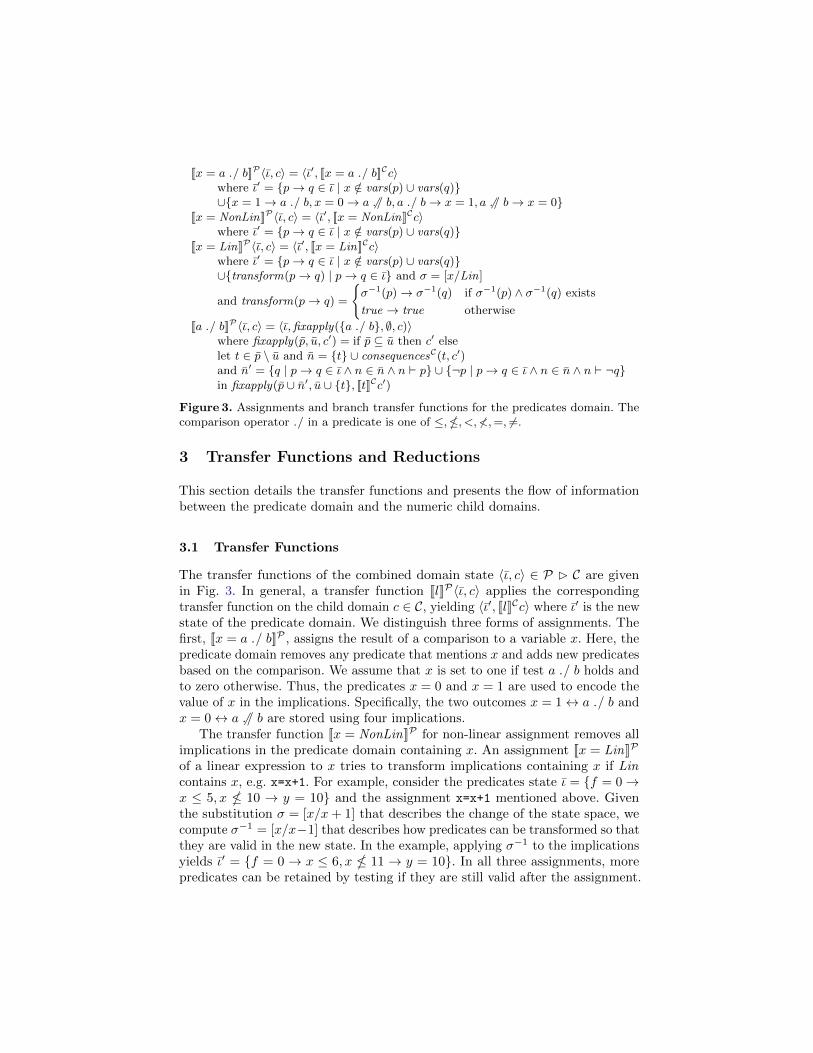
Figure 3. Assignments and branch transfer functions for the predicates domain. Thecomparison operator ./ in a predicate is one of ≤,�, <,≮,=, 6=.

3 Transfer Functions and Reductions

This section details the transfer functions and presents the flow of informationbetween the predicate domain and the numeric child domains.

3.1 Transfer Functions

The transfer functions of the combined domain state 〈ι, c〉 ∈ P B C are givenin Fig. 3. In general, a transfer function [[l]]P〈ι, c〉 applies the correspondingtransfer function on the child domain c ∈ C, yielding 〈ι′, [[l]]Cc〉 where ι′ is the newstate of the predicate domain. We distinguish three forms of assignments. Thefirst, [[x = a ./ b]]P , assigns the result of a comparison to a variable x. Here, thepredicate domain removes any predicate that mentions x and adds new predicatesbased on the comparison. We assume that x is set to one if test a ./ b holds andto zero otherwise. Thus, the predicates x = 0 and x = 1 are used to encode thevalue of x in the implications. Specifically, the two outcomes x = 1↔ a ./ b andx = 0↔ a 6./ b are stored using four implications.

The transfer function [[x = NonLin]]P for non-linear assignment removes allimplications in the predicate domain containing x. An assignment [[x = Lin]]P

of a linear expression to x tries to transform implications containing x if Lincontains x, e.g. x=x+1. For example, consider the predicates state ι = {f = 0→x ≤ 5, x � 10 → y = 10} and the assignment x=x+1 mentioned above. Giventhe substitution σ = [x/x+ 1] that describes the change of the state space, wecompute σ−1 = [x/x−1] that describes how predicates can be transformed so thatthey are valid in the new state. In the example, applying σ−1 to the implicationsyields ι′ = {f = 0 → x ≤ 6, x � 11 → y = 10}. In all three assignments, morepredicates can be retained by testing if they are still valid after the assignment.

We now consider the transfer function for an assumption [[a ./ b]]P . Theinformation from the test a ./ b is used by the predicate domain to gather furtherfacts about the state. The process of applying these facts to the child domain iscalled reduction [4]. The reduction is performed as a fixpoint computation andcan be seen as an instance of Granger’s framework for reduction by local iteration[8]. Specifically, the function fixapply gathers a set of deduced predicates p anda set of predicates u that have already been used. In each iteration a predicatet ∈ p \ u is applied to the child state c′, yielding [[t]]Cc′. Furthermore, a set of newpredicates that are implied by t are computed in two steps. First, t is combinedwith a set n of semantic consequences which is computed by consequencesC asdetailed below. Second, a set of syntactically implied predicates n′ is computedfrom n by inspecting the implications in the predicate domain. We use modusponens resolution to deduce q from an implication p → q ∈ ι where t ` p anddeduce ¬p if t ` ¬q. Here, the syntactic entailment ` is defined as follows:

Definition 1 (Syntactic Predicate Entailment `). A predicate q is entailedby another predicate p, written as p ` q, if p ≡ q or if p describes a weaker condi-tion that subsumes the condition of q. We use the following syntactic entailmentrules (analogous definitions for the negations of the comparison operators �,≮):

p ` x 6= c if p ∈ {x = c′ | c′ 6= c} ∪ {x ≤ c′ | c′ < c} ∪ {x < c′ | c′ ≤ c}p ` x ≤ c if p ∈ {x = c′ | c′ ≤ c} ∪ {x ≤ c′ | c′ ≤ c} ∪ {x < c′ | c′ − 1 ≤ c}p ` x < c if p ∈ {x = c′ | c′ < c} ∪ {x ≤ c′ | c′ < c} ∪ {x < c′ | c′ ≤ c}

The set of syntactically implied predicates n′ is added to p and, hence,eventually applied to the child state. Since at most two predicates for eachimplication in ι can be added to p, this iterative reduction terminates.

Although not strictly necessary, the consequencesC function allows informationto flow from the child domain to the predicate domain. The function synthesizesnew predicates that become valid after applying the test t. It is different for eachchild domain. An implementation for the interval domain I is as follows:

consequencesI(t, c) = let c′ = [[t]]Ic in {x = l | c(x) 6= c′(x) ∧ c′(x) ∈ [l, l]}

Here, c(x) is the interval of the variable x in the state c. The insight inthis definition is that the only additional information inferable by the intervaldomain is that a variable x may have become constant due to a test such asx ≤ c. Returning these equality predicates may allow additional deductions inthe predicate domain. Note that other child domains may deduce different facts.

3.2 Example for the Reduction after Executing Assumptions

We illustrate the reduction when applying an assumption [[a ./ b]]P using anexample. Consider applying the test f < 1 to the state s = 〈ι, c〉 that consistsof the predicates ι ∈ P and the intervals c ∈ I as child domain. Let ι = {f =0 → x ≤ 0} and c = {f ∈ [0, 1], x ∈ [−1, 1]}. The first step in the transferfunction is to infer the consequences of the test: n = consequencesI(f < 1, c).As the child state becomes c′ = {f ∈ [0, 0], x ∈ [−1, 1]}, the consequences are

n = {f = 0}. The synthesized predicate in n syntactically entails the left-handside of the implication f = 0→ x ≤ 0 that is tracked in the predicate domain.Thus, fixapply calls itself recursively with the new predicate x ≤ 0 which resultsin a call to consequencesI(x ≤ 0, c′) = ∅. Now, the set of implied predicates n′ isempty and a fixpoint is reached since p = u = {f < 1, x ≤ 0}. Thus, the result ofthe transfer function is [[f < 1]]Ps = 〈{f = 0→ x ≤ 0}, {f ∈ [0, 0], x ∈ [−1, 0]}〉.This recursive reduction mechanism implements all required reductions betweenthe predicate and the child domain. The next section illustrates how this reductionmechanism is used to preempt the loss of precision due to convexity.

3.3 Application to Non-Convex Spaces

Reconsider the example in Fig. 1 where a division by zero is prevented by aguard. The problem here is that the state space for d is non-convex and cannotbe expressed with the intervals domain I. However, using the predicate domainP we are able to prove the invariant at program point 4 even though the intervalvalue for d at that point is d ∈ [−2, 2]. We illustrate an analysis of the programfor an initial state where the interval domain tracks d with the value d ∈ [−2, 2].By executing line 1, the four implications for the assignment of a comparisonare added to the predicate domain, yielding the state ι = {f = 1→ d 6= 0, f =0 → d = 0, d 6= 0 → f = 1, d = 0 → f = 0}. On entering the then-branch, thetest f = 1 in line 3 restricts the variable f in the interval domain to f ∈ [1, 1].The predicate domain uses the first implication to deduce d 6= 0, which is alsoapplied to the child domain. However, the child domain I is not able to expressthe disjunction d ∈ [−2,−1] ∨ [1, 2] thus the state after applying d 6= 0 remainsd ∈ [−2, 2]. The assertion in line 4 translates to an edge to the dedicated errornode that is labelled with the test d = 0. Hence, the assertion fails if d = 0 issatisfiable. The predicate domain observes that the right-hand side d 6= 0 ofthe implication f = 1 → d 6= 0 is false and thus adds the negated left-handside f 6= 1 to n′. Once the predicate domain applies f 6= 1 to the child statec = {f ∈ [1, 1], d ∈ [−2, 2]}, the result is ⊥, the unreachable state. Thus, the errornode is not reachable in the program and the assertion is verified even thoughthe convex numeric domain is not precise enough to express d 6= 0. The reductionmechanism is able to exploit the information in the implications for verifyingassertions without requiring more complex (i.e. non-convex) numeric domains.

In general, observing predicates from assignments is only a syntactic techniquethat may fail for more complex disjunctive invariants. The next section thereforeillustrates how the reduction mechanism implemented by fixapply naturallycombines with a more sophisticated way of inferring new implications.

4 Lattice Operations and Predicate Synthesis

We present entailment test, join and widening operations of the predicate domain.Moreover, we introduce a novel synth function that synthesizes new implicationsbetween predicates that counteract the loss of precision in numeric domains.

〈ι1, c1〉 vP 〈ι2, c2〉 = c1 vC c2 ∧ entailed(ι2, ι1, c1) = ι2where entailed(ι′, ι, c) = {p′→q′∈ ι′ | (∃p→q∈ ι.p′` p ∧ q` q′) ∨ ([[p′]]Cc � q′)}

〈ι1, c1〉 tP 〈ι2, c2〉 = 〈join(ι1, ι2) ∪ synthC(c1, c2), c1 tC c2〉where join(ι1, ι2) = entailed(ι1, ι2, c2) ∪ entailed(ι2, ι1, c1)

Figure 4. Lattice operations for the predicate domain.

4.1 Lattice Operations

We commence by detailing the entailment test 〈ι1, c1〉 vP 〈ι2, c2〉 in Fig. 4.It performs the entailment test c1 vC c2 on the child domain and tests if allthe implications in the right argument ι2 are entailed by the left argument bycalling the function entailed(ι′, ι, c). The latter function returns an implicationp′ → q′ ∈ ι′ if it is either syntactically entailed in ι or semantically entailed inthe state c. Semantic entailment � is defined as follows:

Definition 2 (Semantic Predicate Entailment �). A predicate q is entailedin a state c, written c � q, if testing ¬q in c yields an empty state, i.e., [[¬q]]Cc = ⊥.

By this definition, the test [[p′]]Cc � q′ in entailed reduces to checking whether[[¬q′]]C([[p′]]Cc) = ⊥. Thus, if the predicate p′ on the left-hand side of the implica-tion p′ → q′ is false in c then [[¬q′]]C⊥ = ⊥ follows and the implication is entailedin c. The two tests [[·]]C on the child domain c can be avoided if the implicationis syntactically entailed by an implication in ι. Here, the implication p→ q ∈ ιentails p′ → q′ if the premise p′ is stronger and the conclusion q′ is weaker whichis expressed by p′ ` p ∧ q ` q′. Note that neither the syntactic nor the semanticentailment test subsumes the other as both approximate the test differently.

The join 〈ι1, c1〉 tP 〈ι2, c2〉 independently computes a join on the predicatedomain and on the child domain. In oder to join the implication sets ι1 and ι2,we define a function join that keeps all implications that hold in the respectiveother state using the entailed function described above. Note that the semanticentailment test in entailed is particularly important for the join as one of thepredicate domain states may be empty so that the syntactic entailment woulddiscard all implications. The semantic join is able to retain newly inferredpredicates in, for example, loop bodies as illustrated later.

In addition to the predicates returned by the join function, new implicationsare synthesized from the child domain states using the synthC function. The ideais to synthesize implications that characterize the approximation that occurred aspart of the tC operation. Which synthesized implications are generated dependson the numeric domain. If the predicate language is sufficiently expressive, adomain could potentially characterize all precision losses that occur during ajoin. The following synthI function for the interval domain is an example thatgenerates implications for all changing bounds. Moreover, by relating changes ofinterval bounds between different variables, it generates relational informationthat cannot be expressed within the interval domain itself. It is defined as follows:

synthI(c1, c2) = let c = c1 tI c2and m = {x ∈ vars(c1) ∩ vars(c2) | c1(x) 6= c2(x)} and i ∈ {1, 2}and ui = {uxi | x ∈ m ∧ ci(x) ∈ [lxi, uxi] ∧ c(x) ∈ [lx, ux] ∧ uxi < ux}and li = {lxi | x ∈ m ∧ ci(x) ∈ [lxi, uxi] ∧ c(x) ∈ [lx, ux] ∧ lx < lxi}in {ux1<x→ ly2≤y, uy1<y→ lx2≤x | x, y ∈ m ∧ uxi, uyi ∈ ui ∧ lxi, lyi ∈ li}

Let vars(c) return all the variables x ⊆ X tracked in the state c and let c(x)denote the interval of the variable x. The set of variables m that are not equal inboth states are those whose joined value is an approximation of the input intervals.For these variables we compute a set of changing lower and upper bounds li andui whose indices indicate the variable and origin of the bound. For example, whenjoining c1(x) ∈ [0, 5] with c2(x) ∈ [10, 15], resulting in c(x) ∈ [0, 15], the upperbound ux1 = 5 of c1(x) and the lower bound lx2 = 10 of c2(x) are lost whereas theother bounds are retained in c(x). These changing bounds are used for generatingimplications. Specifically, each implication correlates a lost upper bound uxi fromci with a lost lower bound ly(2−i) from c2−i where i = 1, 2. For the exampleabove x = y, thus the only generated implication is ux1 < x → lx2 ≤ x, thatis, 5 < x→ 10 ≤ x. The implication allows that a test such as 7 < x is refinedto 10 ≤ x, thereby recovering the precision loss in the join that is due to theconvexity of the interval domain. In general, the bounds of several variables canbe related, thereby even generating relational information.

One drawback of the definition above is that implications are added for eachpair of variables from m, thus, the returned set of implications is quadraticin |m|. This quadratic growth can be avoided by not generating a redundantimplication a→ c if both a→ b and b→ c are already present. Specifically, bysorting m using some total ordering, we only emit implications over variablesthat are adjacent in this ordering, as well as an implication relating the largestvariable with the smallest. As the predicate domain performs a transitive closureon application of a test predicate (through fixapply), adding only implicationsbetween adjacent variables is sufficient to recover all information expressed in achain of implications. Using this optimization, we are able to reduce the numberof synthesized implications to be linear in the number of changed variables |m|.

Before we consider further examples, we consider the widening operation,defined by, say, 〈ι1, c1〉∇P 〈ι2, c2〉 = 〈join(ι1, ι2) ∪ synthC(c1, c2), c1∇C c2〉. Thisdefinition is analogous to the join operation but applies widening on the childstates c1, c2. One caveat of this definition is that termination is not guaranteed.Consider an implication p′ → q′ at a loop head and assume that a conditionalin the loop refines the child state by using the [[a ./ b]]P transformer in Fig. 3which, in turn, may use the information in p′ → q′. Suppose that joining thetwo branches of the conditional creates a new implication p → q by means ofthe synthC function that is syntactically weaker than p′ → q′. If [[p′]]Cc1 6� q′(the previous implication cannot be shown to hold in the new state) then theloop is not stable. If furthermore [[p]]Cc2 � q (the new implication holds inthe previous state), the loop is analyzed with the new implication. Thus, oneimplication may be replaced by another one, possibly indefinitely so. In order toensure termination, standard widening techniques can be used, such as eventually

c1 c2 synthI(c1, c2) c1 tI c2x ∈ [0,5] [10, 15] {5 < x→ 2 ≤ y, [0, 15]y ∈ [−5,−1] [2, 3] −1 < y → 10 ≤ x} [−5, 3]

Figure 5. The join of two states in the intervals domain I and the synthesized implica-tions correlating the bounds lost due to the convex approximation.

disallowing new implications [15]. This can be implemented by using the definition〈ι1, c1〉∇P 〈ι2, c2〉 = 〈entailed(ι1, ι2, c2), c1∇C c2〉 after k iterations. So far, wewere unable to find examples that exhibit this non-terminating behavior.

4.2 Recovering Precision using Relational Information

One strength of our synthI function is that it creates relational information,that is, it generates implications between different variables. This relationalinformation enables fixapply to deduce, from a test of one variable, more preciseranges for other variables. In particular, a test t that separates two states, i.e.[[t]]Ic1 = c1 and [[t]]Ic2 = ⊥ is enriched by the relational implications so that alllosses due to convexity are recovered, that is, [[t]]P(〈ι1, c1〉 tP 〈ι2, c2〉) = 〈ι′1, c1〉.

We illustrate this ability using two states s1 = 〈∅, {x ∈ [0, 5], y ∈ [−5,−1]}〉and s2 = 〈∅, {x ∈ [10, 15], y ∈ [2, 3]}〉. The joined state s = s1 tP s2 is givenby s = 〈{5 < x → 2 ≤ y,−1 < y → 10 ≤ x}, {x ∈ [0, 15], y ∈ [−5, 3]}〉. Thisoperation is illustrated in Fig. 5 where the bounds in bold are those that are lostand the arrows indicate which bounds are related by the generated implications.We now show how applying the test 0 < y on s recovers the numeric statein s2 and, analogously, that applying y ≤ 0 recovers the numeric state of s1.Specifically, when applying the test 0 < y on state s, the left-hand side of theimplication −1 < y → 10 ≤ x is syntactically entailed, so that 10 ≤ x is alsoapplied to the child state, yielding the precise value [10, 15] for x. The predicate10 ≤ x syntactically entails the other implication 5 < x → 2 ≤ y. Thus, thepredicate 2 ≤ y is applied to the child state, yielding the precise value [2, 3]for y. After that no new predicates are entailed and the recursive predicateapplication in the function fixapply stops with the state s′2 = 〈{5 < x→ 2 ≤ y,−1 < y → 10 ≤ x}, {x ∈ [10, 15], y ∈ [2, 3]}〉. Observe that the interval domain isidentical to that of s2. Analogously, we get a state s′1 in which the interval for xis [0, 5] and for y is [−5,−1] after applying the opposing condition y ≤ 0.

In summary, the predicate domain improves the precision of a child domaintracking precision losses that are reported by the child. In particular, the domain-specific synthC function can generate predicates that cannot be expressed in thedomain itself. This allows the predicate domain to maintain enough disjunctiveinformation to recover the state before the join whenever a test is able to separatethe two states. Note though that there exist cases when this is not completelypossible, namely when the value of x in one state overlaps the value in the otherstate. Consider c1(x) ∈ [0, 4] and c2(x) ∈ [2, 8]. A test x < 3 does not separatethe two states. However, any test outside the overlapping range [2, 4] is able toseparate the two states which, in turn, leads to the refinement of other bounds.

4.3 Application to Path-Sensitive Invariants

This section illustrates how our domain can verify an example taken from [5].The challenge of analyzing the code in Fig. 6a) is that the join of different pathsloses precision and the invariant that a file is only accessed if it was openedbefore cannot be proved. For the sake of presentation, we use open to denotethe value of out->is_open. Note that the assertion in line 3 can be proved byusing the interval domain alone, as open is [1, 1] due to line 2. However, theassertion in line 10 cannot be proved by using intervals alone: observe that openis set to [0, 0] in line 4 and that the join of this value with the value [1, 1] fromline 7 yields the convex approximation of [0, 1] in line 10 of the assertion. As aconsequence, the assertion cannot be proved since the edge to the error statewith assumption open = 0 is satisfiable. Now consider analyzing the exampleusing the predicate domain with the interval domain as child. Then the joinof the then branch in line 7 and the state before line 6 creates an implication0 < flag → 1 ≤ open. When applying the branch condition flag = 1 of line 9,the implied predicate 1 ≤ open is used to reduce the state, yielding open ∈ [1, 1]in the interval domain. Thus, the assertion can be proved since the edge to theerror state with assumption open = 0 is unreachable. The example illustrateshow numeric domains may lose precision when joining paths and, thus, may failto express a path-sensitive invariant which is crucial to prove assertions in thebranch of a conditional.

Fischer et al. [5] prove the assertion in line 10 by not joining the statesafter the conditional in line 6, thus keeping the states where open = 0 andopen = 1 separate. They associate a predicate with a numeric state and joinnumeric states only if they are associated with the same predicate. Thus, theirabstract state before the conditional in line 9 is {〈flag = 0, open ∈ [0, 0]〉, 〈flag =1, open ∈ [1, 1]〉} which reduces to {〈flag = 1, open ∈ [1, 1]〉} inside the conditional.Although their approach is able to prove the assertion, it is more costly as it tracksseveral numeric states. Although using sharing can reduce the resource overheadof tracking multiple states [11] the cost of tracking several states is generallyhigher [14]. Our approach retains the conciseness of a single convex numericstate and merely adds the implications necessary to express certain disjunctiveinformation. In particular, we only infer disjunctive information for variablesthat actually differ in the join of two numeric states rather than duplicating theinformation on all variables.

4.4 Application to Separation of Loop Iterations

A particularly challenging example from the literature [12] requires that variablevalues of certain loop iterations are distinguished. The example in Fig. 6b) isprototypical for a loop that frees a memory region in its last iteration. Theassertion in line 4 expresses that the memory region pointed-to by p has not yetbeen deallocated. In order to prove this assertion, an analysis needs to separatethe value of the pointer p in the last loop iteration from its value in all previousiterations. In particular, the example is difficult to prove using convex numeric

a)1 FILE *out;

2 out ->is_open = 1;

3 assert(out ->is_open == 1);

4 out ->is_open = 0;

5 ...

6 if (flag)

7 out ->is_open = 1;

8 ...

9 if (flag)

10 assert(out ->is_open == 1);

b)1 p = &some_var;

2 n = 5;

3 while (n >= 0) {

4 assert(p != 0);

5 // dereference p

6 ...

7 if (n == 0)

8 p = 0;

9 n--;

10 }

Figure 6. Two challenging examples from the literature: a) accessing a file only if itwas already opened and b) freeing a pointer in the last loop iteration.

domains due to a precision loss that occurs when joining the point 〈p, n〉 = 〈0,−1〉at line 10 of the last loop iteration with the earlier states where p 6= 0 and n ≥ 0.

However, using the simple interval numeric domain and our predicate domain,the example is proved using the fixpoint computation detailed in Fig. 7. In step 1of the table, p is initialized to a non-zero address of a variable, which we illustrateby using the value 99. After initializing the loop counter n in step 2, the loop isentered as the loop condition n >= 0 is satisfied. In step 5, it is determined thatthe then-branch in line 8 is not reachable. After decrementing n, the state ispropagated to the loop head via the back-edge in step 8. At this point, wideningis applied. Additional heuristics [15] ensure that the interval [−1, 5] is tried for n,rather than widening n immediately to [−∞, 5]. By applying the loop conditionn >= 0, a new state for the loop body is obtained in step 9. In step 12, it isobserved that the then-branch in line 8 is reachable. In the next step in line 9 thestates of both branches are joined and the interval domain approximates p with[0, 99]. In the same step, the implications 0 < n → 99 ≤ p, 0 < p → 0 ≤ n aresynthesized. In step 14 these predicates are transformed using σ−1 = [n/n+ 1].This state is joined with the previous state at the loop header at step 15. Ourwidening heuristic suppresses widening since a new branch in the program hasbecome live [15]. Since the resulting numeric state has changed due to the newvalue of p, the fixpoint computation continues. Note that during the join in step 15,both implications −1 < n→ 99 ≤ p, 0 < p→ −1 ≤ n are semantically entailedin the current state at the loop head (as computed in step 8’) and therefore keptin the joined state. Evaluating the loop condition in step 16 enforces that n ≥ 0,that is, 0 ≤ n. The latter predicate syntactically entails the predicate −1 < n.Thus, the fixapply function deduces that 99 ≤ p holds, yielding p ∈ [99, 99]. Theassertion holds since intersecting the state at step 16 with p = 0 yields ⊥. Thus,at line 4, p cannot be 0 and the assertion holds. Continuing the analysis of theloop observes a fixpoint in step 22. Note that the assertion can also be shownwhen using standard widening that sets n to [−∞, 0] in step 8’. However, for thesake of presentation, we illustrated the example with the more precise states.

step line intervals implicationsp n

1 2 [99, 99]2 3 [99, 99] [5, 5]3 4 [99, 99] [5, 5]· · · · · · · · ·5 7 [99, 99] [5, 5]6 9 [99, 99] [5, 5]7 10 [99, 99] [4, 4]8 3 t [99, 99] [4, 5]8’ 3’ ∇ [99, 99] [−1, 5]9 4 [99, 99] [0, 5]· · · · · · · · ·12 8 [99, 99] [0, 0]13 9 t [0, 99] [0, 5] {0 < n→ 99 ≤ p, 0 < p→ 0 ≤ n}14 10 [0, 99] [−1, 4] {−1 < n→ 99 ≤ p, 0 < p→ −1 ≤ n}15 3 t [0, 99] [−1, 5] {−1 < n→ 99 ≤ p, 0 < p→ −1 ≤ n}16 4 [99, 99] [0, 5] {−1 < n→ 99 ≤ p, 0 < p→ −1 ≤ n}· · · · · · · · ·22 3 v [0, 99] [−1, 5] {−1 < n→ 99 ≤ p, 0 < p→ −1 ≤ n}

Figure 7. States during the analysis of the loop example in Fig. 6b).

benchmark suite programs lines lines avg. time avg. time avg. (P) time avg. (D)

literature 9 9–17 14 ms 38 ms 99 ms 381 mstest 8 66–274 115 ms 393 ms 1658 ms -

Figure 8. Evaluation of our implementation. Due to technical reasons, the “test”benchmark suite could not be analyzed using the disjunctive domain (D).

5 Related Work and Evaluation

The Predicate abstract domain was inspired by a weaker domain that trackedbi-implications of the form f ↔ x ≤ c [18]. This domain is useful in the analysisof machine code where conditional branches are encoded using two separateinstructions. The first instruction is a comparison that stores the result of x ≤ c ina processor flag f . The second instruction is a branch instruction that determinedthe jump target based on f . By tracking an association between the comparisonresult f and the predicate x ≤ 0, the edge of the jump with the assumption f = 1can be made more precise by also assuming x ≤ 0 and analogously for f = 0.However, the use of simple bi-implications only states additional invariants ratherthan predicates that hold conditionally. Hence, disjunctive information cannotbe described by using only bi-implications.

We evaluated our combined predicate/numeric domain on several examplesin the literature, including the ones presented in this paper, shown as “literature”in Fig. 8. We also evaluated larger examples shown as “test”. All examples fromthe literature required the predicate domain to verify except for the examplein Fig. 1 that our weaker predicate domain [18] already handles. The times areshown when running without and with the predicate domain “(P)”. The lastcolumn shows the running time with a disjunctive domain “(D)” that tracksdifferent numeric states depending on the index ranges of a loop [6,15]. Due tothis, only one example in the “literature” benchmark suite could possibly profit.A precision comparison of our disjunctive and the predicate domain can thereforenot be conclusive for the various disjunctive domains in the literature [11,14].

5.1 Related Work

The idea of abstracting a system relative to a set of predicates was first applied byGraf and Saıdi to state graphs created during model checking [7]. This approachhas later been generalized to software model checking by Ball et al. [1]. Here, anabstraction tool c2bp translates a C program to a program over Boolean variables.The value of a Boolean variable is true if the corresponding predicate holds inthe input C program. The universe of possible predicates is very large as thesemantics of each assignment and test is expressed by predicates. For scalability,c2bp abstracts the input C program only with respect to a few predicates. Theidea of counter-example driven refinement is to increase this set of predicatesby deducing which additional predicates are needed to discharge a verificationcondition. This deduction is performed on a path through the program on whichthe current Boolean abstraction is insufficient to prove a verification condition.There are two ways in which this refinement may fail: Firstly, the translationof C statements and tests into predicates may be inaccurate or the logic of thepredicates may be insufficient to represent the C semantics precisely. Secondly,a set of predicates that suffices to discharge the verification condition on thechosen path may be insufficient when considering the whole program.

An abstract interpretation over domains that lose precision due to convexityis naturally improved by avoiding the computation of joins. This approach iscommonly known as disjunctive completion [4]. In practice, the disjunctionsare qualified by a set of predicates and are stored in a binary decision-diagram(BDD) where decision nodes are labeled with predicates and the leaves are convexnumeric abstract domains [11,14]. The challenge in implementing these domainsis that evaluation of transfer functions in one leaf may lead to a result that hasto be propagated to many other leaves. A particular challenge is the wideningoperator and the reduction between predicates and states [10,15]. One drawbackof using a BDD as state is that computing a fixpoint of a loop will performall operations on each leaf of the BDD, even those that are stable within, say,the current loop. This can be avoided by lifting the fixpoint computation fromtracking a map P → S to P × C → S where P are program points, S are statesand C is a context. By using the predicates on a path in the decision diagramas context, the whole decision tree can be encoded by using one context perpath. The advantage of this encoding is that stable leaves in the original decisiontree are no longer propagated since they are each checked for stability by thefixpoint engine [17]. Using predicates as context can be seen as an elegant way ofduplicating the CFG which is a technique often used to improve widening [6].

Beyer et al. combine abstract domains with predicates [2]. Their frameworkassociates a precision level Π with each domain that can be adjusted based onobserved values in the program. A value-set analysis, for instance, may specifythat only variables with less than five values are tracked while a predicate domainwill store the set of possible predicates in Π. They propose to change this precisionlevel during the analysis, so that a precision loss in one domain can be met witha precision increase in another. They instantiate their framework by an analysisthat switches from tracking value sets to tracking predicates once the former

becomes too expensive. Their states are tuples of the precision levels and thedomain states so that a different domain state is tracked for each precisionlevel. Their approach thereby resembles the disjunctive completion approachesdiscussed earlier. Interestingly, they propose the use of a function abstract tosynthesize predicates from an abstract state. However, in their implementation itonly returns predicates occurring in the current program.

Further afield are techniques to refine abstract interpretations based oncounter examples [13,9]. The idea here is to re-run the abstract interpretationonce a verification condition cannot be discharged. An improved precision ofthe abstract interpreter is obtained by improving the widening or the abstractstate based on the path of the counter example. Our work can be seen as dual tocounterexample-driven refinement as we employ predicates to avoid a precisionloss rather than to refine a state that is too coarse. An approach that usescounterexample-driven refinement and which is seemingly close to ours is thatof Fischer et al. [5] who propose a domain containing a map from a predicateto a numeric abstract domain. Like our setup, their construction is a reducedcardinal power domain [4] or, more generally, a co-fibered domain [20]. However,since they track one numeric abstract domain for each predicate, there is nobound on the number of states that they infer. Future work should address iftheir techniques can be incorporated into our abstract domain, that is, if newpredicates can be synthesized without duplicating the numeric state.

Interestingly, when state spaces are bounded, disjunctive invariants can beencoded using integral polyhedra [19]. However, since even rational polyhedraare expensive, storing disjunctive information explicitly seems to be preferable.

5.2 Conclusion

We presented a co-fibered domain that tracks implications between predicates.This domain takes a single numeric abstract domain as child and thereby avoidstracking several child domains which is the most prominent way to encodedisjunctive information. We illustrated that our domain solves challenging verifi-cation examples form the literature while using a simple deduction and reductionmechanism in form of the two novel functions synth and fixapply , respectively.

References

1. T. Ball, R. Majumdar, T. Millstein, and S. K. Rajamani. Automatic PredicateAbstraction of C Programs. In Programming Languages, Design and Implementation,pages 203–213. ACM, 2001.

2. D. Beyer, T. Henzinger, and G. Theoduloz. Program analysis with dynamic precisionadjustment. In Automated Software Engineering, 2008.

3. B. Blanchet, P. Cousot, R. Cousot, J. Feret, L. Mauborgne, A. Mine, D. Monniaux,and X. Rival. A Static Analyzer for Large Safety-Critical Software. In ProgrammingLanguage Design and Implementation, San Diego, USA, June 2003. ACM.

4. P. Cousot and R. Cousot. Systematic Design of Program Analysis Frameworks. InPrinciples of Programming Languages, pages 269–282, San Antonio, Texas, USA,January 1979. ACM.

5. J. Fischer, R. Jhala, and R. Majumdar. Joining Dataflow with Predicates. InM. Wermelinger and H. Gall, editors, European Software Engineering Conference,volume 30, pages 227–236. ACM, September 2005.

6. D. Gopan and T. W. Reps. Guided Static Analysis. In H. R. Nielson and G. File,editors, Static Analysis Symposium, volume 4634 of LNCS, pages 349–365, KogensLyngby, Denmark, August 2007. Springer.

7. S. Graf and H. Saidi. Construction of abstract state graphs with PVS. In O. Grum-berg, editor, Computer Aided Verification, volume 1254 of LNCS, pages 72–83.Springer, 1997.

8. P. Granger. Improving the Results of Static Analyses of Programs by Local Decreas-ing Iterations. In R. Shyamasundar, editor, Foundations of Software Technologyand Theoretical Comp. Sci., volume 652 of LNCS, pages 68–79. Springer, 1992.

9. B. S. Gulavani and S. K. Rajamani. Counterexample Driven Refinement forAbstract Interpretation. In Holger Hermanns and Jens Palsberg, editors, Tools andAlgorithms for the Construction and Analysis of Systems, volume 3920 of LNCS,pages 474–488, Vienna, Austria, March 2006. Springer.

10. A. Gurfinkel and S. Chaki. Boxes: A Symbolic Abstract Domain of Boxes. InR. Cousot and M. Martel, editors, Static Analysis Symposium, volume 6337 ofLNCS, pages 287–303. Springer, 2010.

11. A. Gurfinkel and S. Chaki. Combining Predicate and Numeric Abstraction forSoftware Model Checking. Software Tools for Techn. Transfer, 12(6):409–427, 2010.

12. M. Heizmann, J. Hoenicke, and A. Podelski. Software Model Checking for PeopleWho Love Automata. In N. Sharygina and H. Veith, editors, Computer AidedVerification, volume 8044 of LNCS, pages 36–52. Springer, July 2013.

13. R. Leino and F. Logozzo. Loop Invariants on Demand. In K. Yi, editor, AsianSymposium on Programming Languages and Systems, volume 3780 of LNCS, pages119–134, Tsukuba, Japan, 2005. Springer.

14. L. Mauborgne and X. Rival. Trace Partitioning in Abstract Interpretation BasedStatic Analyzers. In M. Sagiv, editor, European Symposium on Programming,volume 3444 of LNCS, pages 5–20, Edinburgh, UK, April 2005. Springer.

15. B. Mihaila, A. Sepp, and A. Simon. Widening as Abstract Domain. In NASAFormal Methods, volume 7871 of LNCS, pages 170–186, Moffett Field, California,USA, May 2013. Springer.

16. M. Peron and N. Halbwachs. An Abstract Domain Extending Difference-BoundMatrices with Disequality Constraints. In B. Cook and A. Podelski, editors,Verification, Model Checking, and Abstract Interpretation, volume 4349 of LNCS,pages 268–282, Nice, France, January 2007. Springer.

17. S. Sankaranarayanan, F. Ivancic, I. Shlyakhter, and A. Gupta. Static Analysisin Disjunctive Numerical Domains. In Kwangkeun Yi, editor, Static AnalysisSymposium, volume 4134 of LNCS, pages 3–17, Seoul, Korea, August 2006. Springer.

18. A. Sepp, B. Mihaila, and A. Simon. Precise Static Analysis of Binaries by Extract-ing Relational Information. In M.Pinzger and D. Poshyvanyk, editors, WorkingConference on Reverse Engineering, Limerick, Ireland, October 2011. IEEE.

19. A. Simon. Splitting the Control Flow with Boolean Flags. In M. Alpuente andG. Vidal, editors, Static Analysis Symposium, volume 5079 of LNCS, pages 315–331,Valencia, Spain, July 2008. Springer.

20. A. Venet. Abstract Cofibered Domains: Application to the Alias Analysis ofUntyped Programs. In Static Analysis Symposium, LNCS, pages 366–382, London,UK, 1996. Springer.