an aerocom initial assessment – optical properties in

Atmos. Chem. Phys., 6, 1815–1834, 2006www.atmos-chem-phys.net/6/1815/2006/© Author(s) 2006. This work is licensedunder a Creative Commons License.

AtmosphericChemistry

and Physics

An AeroCom initial assessment – optical properties in aerosolcomponent modules of global models

S. Kinne1, M. Schulz2, C. Textor2, S. Guibert2, Y. Balkanski2, S. E. Bauer3, T. Berntsen4, T. F. Berglen4, O. Boucher5,6,M. Chin 7, W. Collins8, F. Dentener9, T. Diehl10, R. Easter11, J. Feichter1, D. Fillmore8, S. Ghan11, P. Ginoux12,S. Gong13, A. Grini 4, J. Hendricks14, M. Herzog12, L. Horowitz 12, I. Isaksen4, T. Iversen4, A. Kirkev ag4, S. Kloster1,D. Koch3, J. E. Kristjansson4, M. Krol 16, A. Lauer14, J. F. Lamarque8, G. Lesins17, X. Liu 15, U. Lohmann18,V. Montanaro19, G. Myhre4, J. E. Penner15, G. Pitari19, S. Reddy12, O. Seland4, P. Stier1, T. Takemura20, and X. Tie8

1Max-Planck-Institut fur Meteorologie, Hamburg, Germany2Laboratoire des Sciences du Climat et de l’environnement, Gif-sur-Yvette, France3The Earth Institute at Columbia University, New York, NY, USA4University of Oslo, Department of Geosciences, Oslo, Norway5Laboratoire d’Optique Atmosph’erique, USTL/CNRS, Villeneuve d’Ascq, France6Hadley Centre, Met Office, Exeter, UK7NASA Goddard Space Flight Center, Greenbelt, MD, USA8NCAR, Boulder, Colorado, USA9EC, Joint Research Centre, IES, Climate Change Unit, Ispra, Italy10Goddard Earth Sciences and Technology Center, UMBC, Baltimore, MD, USA11Batelle, Pacific Northwest National Laboratory, Richland, USA12NOAA, Geophysical Fluid Dynamics Laboratory, Princeton, NJ, USA13ARQM Meteorological Service Canada, Toronto, Canada14DLR, Institut fur Physik der Atmosphare, Oberpfaffenhofen, Germany15University of Michigan, Ann Arbor, MI, USA16Institute for Marine and Atmospheric Research Utrecht (IMAU) Utrecht, The Netherlands17Dalhousie University, Halifax, Canada18ETH Zurich, Switzerland19Universita degli Studi L’Aquila, L’Aquila, Italy20Kyushu University, Fukuoka, Japan

Received: 25 May 2005 – Published in Atmos. Chem. Phys. Discuss.: 8 September 2005Revised: 6 February 2006 – Accepted: 13 February 2006 – Published: 29 May 2006

Abstract. The AeroCom exercise diagnoses multi-component aerosol modules in global modeling. In an ini-tial assessment simulated global distributions for mass andmid-visible aerosol optical thickness (aot) were comparedamong 20 different modules. Model diversity was also ex-plored in the context of previous comparisons. For the com-ponent combined aot general agreement has improved for theannual global mean. At 0.11 to 0.14, simulated aot valuesare at the lower end of global averages suggested by remotesensing from ground (AERONET ca. 0.135) and space (satel-lite composite ca. 0.15). More detailed comparisons, how-ever, reveal that larger differences in regional distribution andsignificant differences in compositional mixture remain. Of

Correspondence to:S. Kinne([email protected])

particular concern are large model diversities for contribu-tions by dust and carbonaceous aerosol, because they leadto significant uncertainty in aerosol absorption (aab). Sinceaot and aab, both, influence the aerosol impact on the radia-tive energy-balance, the aerosol (direct) forcing uncertaintyin modeling is larger than differences in aot might suggest.New diagnostic approaches are proposed to trace model dif-ferences in terms of aerosol processing and transport: Theseinclude the prescription of common input (e.g. amount, sizeand injection of aerosol component emissions) and the use ofobservational capabilities from ground (e.g. measurementsnetworks) or space (e.g. correlations between aerosol andclouds).

Published by Copernicus GmbH on behalf of the European Geosciences Union.

1816 S. Kinne et al.: An AeroCom initial assessment

1 Introduction

Aerosol is one of the key properties in simulations of theEarth’s climate. Model-derived estimates of anthropogenicinfluences remain highly uncertain (IPCC, Houghton et al.,2001) in large part due to an inadequate representation ofaerosol. Aerosol originates from diverse sources. Source-strength varies by region and often by season. In addition,aerosol has a short lifetime on the order of a few days. Thus,concentration, size, composition, shape, water uptake and al-titude of aerosol are highly variable in space and time. In re-cent years worldwide parallel efforts have resulted in new ap-proaches for aerosol representation and aerosol processing.Common to most of these approaches is a discrimination ofaerosol in at least five aerosol components: sulfate, organiccarbon, black carbon, mineral dust and sea-salt. This stratifi-cation is desirable for a better characterization of aerosol ab-sorption and size. Aerosol sizes that primarily impact radia-tive energy budgets of the atmosphere are those of the coarsemode (diameters>1µm) and of the accumulation mode (di-ameters between 0.1 and 1.0µm) Sea-salt and dust contri-butions dominate the coarse size mode, while the accumula-tion size mode is characterized by sulfate and carbonaceousaerosol. Hereby it is common practice to stratify carbon con-tributions into strong absorbing soot (black carbon) and intopredominantly scattering organic matter (with sulfate similaroptical properties). The separate processing of these aerosoltypes added complexity and required new assumptions. Totest the skill of new aerosol modules beyond selective com-parisons to processed remote sensing data, modeling groupsjoined the aerosol module evaluation effort called AeroCom.This paper introduces goals and activities of AeroCom andsummarizes aspects of diversity in global aerosol modelingas of 2005 – also intended to establish a benchmark on whichto measure improvements of future modeling efforts. The pa-per presents results with regard to optical properties from thefirst AeroCom experiment (Experiment A), which representsthe models “as they are”. More details on “Experiment A”model diversity, including a comprehensive analysis of bud-gets for aerosol mass and processes are given in companionpaper by Textor et al. (2006).

2 AeroCom

AeroCom intends to document differences of aerosol com-ponent modules of global models and to assemble data-setsfor model evaluations. Overall goals are (1) the identificationof weaknesses of any particular model and of modeling as-pects in general and (2) an assessment of actual uncertaintiesfor aerosol optical properties and for the associated radiativeforcing. AeroCom is open to any global modeling group withdetailed aerosol modules and encourages their participation.AeroCom also seeks the participation of groups, which pro-vide data-sets on aerosol properties. AeroCom assists in data

quality assessments, data combination and in data extensionto the temporal and spatial scales of global modeling.

In order to perform model-intercomparisons and compar-isons to measurement based data AeroCom requests detailedmodel-output and provides a graphical evaluation environ-ment for participants through its websitehttp://nansen.ipsl.jussieu.fr/AEROCOM. The website also lists the presenta-tions of the initial four workshops held at Paris (June 2003),Ispra (March 2004), New York (December 2004) and Oslo(June 2005). These regular workshops are organized (1) tocoordinate activities, (2) to encourage interactions amongmodeling groups and (3) to engage communications betweenmodeling and measurement groups on data-needs and data-quality.

A common data-protocol has been established and wasdistributed to the participants in spring 2003 (see also Aero-Com website). Model-output requests are primarily tailoredto allow budget analysis and comparisons to available data.Additional requests are included to explore details on modelspecific assumptions and processes, such as size distribution,surface wind speed, precipitation, aerosol water or dailycloud fraction and radiative forcing. Several consecutiveexperiments have been proposed to explore diversity inglobal modeling on the path towards improved aerosoldirect and aerosol indirect forcing estimates. At this stagefour experiments have been defined and output requests aresummarized in Table 1.

Experiment A: Modelers are asked to run models in theirstandard configuration. Model output is requested eitherfrom climatological runs (averaged for 3–10 years) or fromsimulations constrained by the meteorological fields for theyears 1996, 1997, 2000 and 2001, with preference on 2000.

Experiment B: Modelers are asked to use AeroCom’sprescribed emission sources for the year 2000 and (whenpossible) meteorological fields for the year 2000. Theadditional request to extend simulations into the first twomonths of the year 2001 will allow comparison to TERRAsatellite data for a complete yearly cycle.

Experiment Pre: Modelers are asked to repeat Exper-iment B now using AeroCom’s prescribed emission sourcesfor the year 1750 rather than for the 2000. Radiative forcingcalculations are asked with priority for the experiments Band PRE.

Experiment Indi : Modelers are asked to conduct model-sensitivity studies to better quantify uncertainties regardingthe aerosol impact on the hydrological cycle with particularconstraints to baseline conditions (e.g. aerosol mass and/orsize), parameterizations (e.g. aerosol impact on the clouddroplet concentration or precipitation efficiency) or effects(e.g. aerosol heating).

Atmos. Chem. Phys., 6, 1815–1834, 2006 www.atmos-chem-phys.net/6/1815/2006/

http://nansen.ipsl.jussieu.fr/AEROCOM

http://nansen.ipsl.jussieu.fr/AEROCOM

S. Kinne et al.: An AeroCom initial assessment 1817

Table 1. Mandatory (X) and optional (o) output requests for the initial four experiments.

Specification subpage on AeroCom web Exp A Exp B Exp Pre Exp Indi

Daily /protocoldaily.html X XMonthly /protocolmonthly.html X X XForcing /protocolforcing.html X X Xindirect – basic /protocolindirectforcing.html X X Oindirect – full /INDIRECT/indirectprotocol.html X

Table 2. Global models with aerosol component modules participating in model assessments.

AeroCom ID Model Type res (deg) lev period data Authors

LO LOA LMDzT at LOA GCM 3.8/2.5 19 yr 2000 all Reddy/BoucherLS LSCE LMDzT at LSCE GCM 3.8/2.5 19 yr 2000 all Schulz/BalkanskiUL ULAQ ULAQat L’Aquila CTM 22.5/10 26 yr 2000 all Pitari/MontanaroSP KYU SPRINTARS at KYU GCM 1.1/1.1 20 yr 2000 all TakemuraCT ARQM GCM III at Toronto GCM 2.8/2.8 32 yr 2000 all GongMI PNNL MIRAGE 2 at PNNL GCM 2.5/2.0 24 1 yr avg all Ghan/EasterEH MPI-HAM ECHAM5.2 MPI-Met GCM 1.8/1.8 31 3 yr avg all Stier/FeichterNF MATCH MATCH 4.2 at NCAR CTM 1.9/1.9 28 yr 2000 all Fillmore/CollinsOT UIO CTM CTM 2 at Oslo Univ CTM 2.8/2.8 40 yr 2000 all Myhre et al.OG UIO GCM CCM3.2 at Oslo Univ. GCM 2.8/2.8 18 3 yr avg all Iversen et al.IM UMI IMPACT at U. Mich CTM 2.5/2.0 30 yr 2000 all Liu/PennerGM MOZGN MOZART 2.5, GFDL CTM 1.9/1.9 28 yr 2000 all Ginoux/HorowitzGO GOCART GOCART 3.1b, GSFC CTM 2.0/2.5 30 yr 2000 all Chin/DiehlGI GISS Model E at GISS GCM 4.0/5.0 20 yr 2000 all Koch/BauerTM TM5 TM5 at Utrecht CTM 4.0/6.0 25 yr 2000 all Krol/DentenerEM DLR ECHAM 4 at DLR GCM 3.8/3.8 19 10 yr avg m Lauer/HendricksGR GRANTOUR, U.Mich CTM 5.0/5.0 1 yr avg m,aot Herzog/PennerNM MOZART at NCAR CTM 1.9/1.9 1 yr avg m,aot Tie/BrasseurNC CAM at NCAR CTM 2.8/2.8 26 1 yr avg all MahowaldEL ECHAM4, Dalh.Univ. GCM 3.8/3.8 3 yr avg m,aot Lesins/Lohmann

note: only models with AeroCom IDs have submitted data according to the AeroCom request, definition: GCM - Global Circulation model(nudging preferred), CTM - Chemical Transport Model

A future intention of the AEROCOM initiative is that theleast constrained “Experiment A” can be revisited to quantifyimprovements by future efforts in aerosol modeling. Moreinsights on differences in aerosol modeling are expectedfrom “Experiment B”, where model input is harmonized interms of aerosol emissions for the year 2000. “ExperimentPre” is the counterpart to “Experiment B”, as it provides thereference in estimates of anthropogenic contributions and as-sociated forcing. A comparison and a general assessment offorcing simulations on the basis of these experiments is sum-marized in Schulz et al. (2006). The prescribed AeroCom(component) emissions for “Experiment B” and “ExperimentPre” can be downloaded atftp://ftp.ei.jrc.it/pub/Aerocom/.The choices made to arrive at a harmonized emission dataset for all major aerosol components are explained in moredetail in Dentener et al. (2006). “Experiment Indi” is dif-ferent in that it investigates the sensitivity of modeling and

the model diversity of processes and parameterizations es-sential to estimates of the aerosol indirect effect. Detailscan be found underhttp://nansen.ipsl.jussieu.fr/AEROCOM/INDIRECT/indirectprotocol.html.

3 Results

The database consists now of results from twenty modelinggroups. Table 2 lists the 16 “Experiment A” AeroCom partic-ipants, who submitted full datasets and 4 contributors, whosubmitted at an earlier stage (e.g. in Kinne et al., 2003) orprovided only partial information.

Here, only results of “Experiment A” are explored, prefer-ably those for the year 2000. Submissions to the three otherexperiments at this stage are incomplete or in preparation.Simulated properties for aerosol optical thickness (aot) and

www.atmos-chem-phys.net/6/1815/2006/ Atmos. Chem. Phys., 6, 1815–1834, 2006

ftp://ftp.ei.jrc.it/pub/Aerocom/

http://nansen.ipsl.jussieu.fr/AEROCOM/INDIRECT/indirect_protocol.html

http://nansen.ipsl.jussieu.fr/AEROCOM/INDIRECT/indirect_protocol.html


8

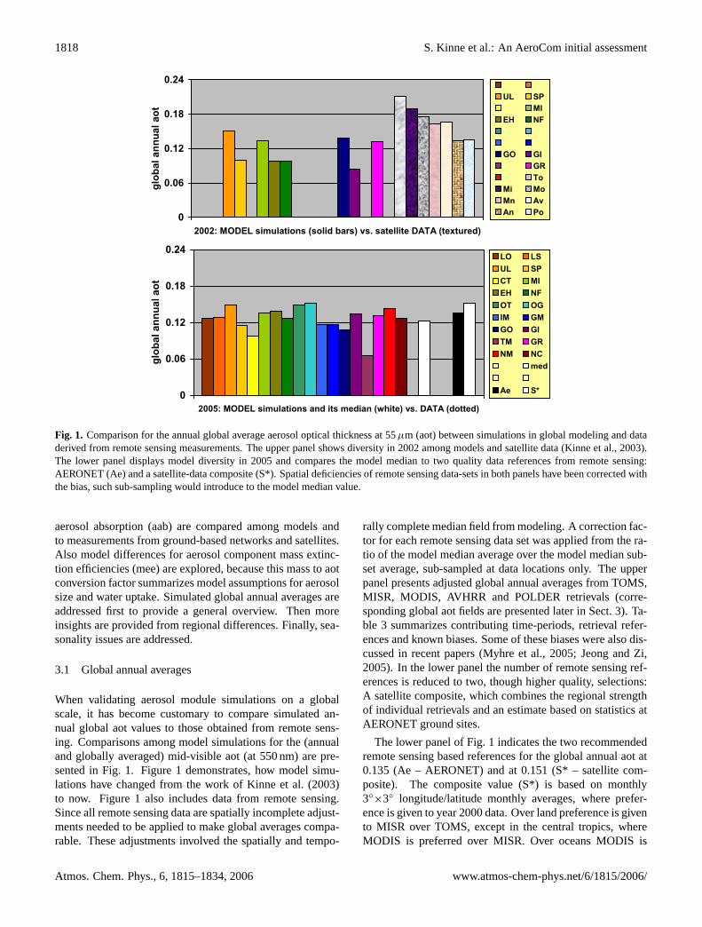
Figure 1. Comparison for the annual global average aerosol optical thickness at .55µm (aot) between simulations in global modeling and data derived from remote sensing measurements. The upper panel shows diversity in 2002 among models and satellite data (Kinne et al 2003). The lower panel displays model diversity in 2005 and compares the model median to two data references from remote sensing: AERONET (Ae) and a satellite-data composite (S*). Spatial deficiencies of remote sensing data-sets in both panels have been corrected with the bias, such sub-sampling would introduce to the model median value.

The lower panel of Figure 1 indicates the two recommended remote sensing based references

for the global annual aot at 0.135 (Ae - AERONET) and at 0.151 (S* - satellite composite).

The composite value (S*) is based on monthly 3ox 3o longitude/latitude monthly averages,

where preference is given to year 2000 data. Over land preference is given to MISR over

TOMS, except in the central tropics, where MODIS is preferred over MISR. Over oceans

MODIS is preferred over AVHRR-1ch, whereas this order in reversed at mid-(to high)

0

0.06

0.12

0.18

0.24

2002: MODEL simulations (solid bars) vs. satellite DATA (textured)

glob

al a

nnua

l aot

UL SPMI

EH NF

GO GIGRTo

Mi MoMn AvAn Po

0

0.06

0.12

0.18

0.24

2005: MODEL simulations and its median (white) vs. DATA (dotted)

glob

al a

nnua

l aot

LO LSUL SPCT MIEH NFOT OGIM GMGO GITM GRNM NC

med

Ae S*

Fig. 1. Comparison for the annual global average aerosol optical thickness at 55µm (aot) between simulations in global modeling and dataderived from remote sensing measurements. The upper panel shows diversity in 2002 among models and satellite data (Kinne et al., 2003).The lower panel displays model diversity in 2005 and compares the model median to two quality data references from remote sensing:AERONET (Ae) and a satellite-data composite (S*). Spatial deficiencies of remote sensing data-sets in both panels have been corrected withthe bias, such sub-sampling would introduce to the model median value.

aerosol absorption (aab) are compared among models andto measurements from ground-based networks and satellites.Also model differences for aerosol component mass extinc-tion efficiencies (mee) are explored, because this mass to aotconversion factor summarizes model assumptions for aerosolsize and water uptake. Simulated global annual averages areaddressed first to provide a general overview. Then moreinsights are provided from regional differences. Finally, sea-sonality issues are addressed.

3.1 Global annual averages

When validating aerosol module simulations on a globalscale, it has become customary to compare simulated an-nual global aot values to those obtained from remote sens-ing. Comparisons among model simulations for the (annualand globally averaged) mid-visible aot (at 550 nm) are pre-sented in Fig. 1. Figure 1 demonstrates, how model simu-lations have changed from the work of Kinne et al. (2003)to now. Figure 1 also includes data from remote sensing.Since all remote sensing data are spatially incomplete adjust-ments needed to be applied to make global averages compa-rable. These adjustments involved the spatially and tempo-

rally complete median field from modeling. A correction fac-tor for each remote sensing data set was applied from the ra-tio of the model median average over the model median sub-set average, sub-sampled at data locations only. The upperpanel presents adjusted global annual averages from TOMS,MISR, MODIS, AVHRR and POLDER retrievals (corre-sponding global aot fields are presented later in Sect. 3). Ta-ble 3 summarizes contributing time-periods, retrieval refer-ences and known biases. Some of these biases were also dis-cussed in recent papers (Myhre et al., 2005; Jeong and Zi,2005). In the lower panel the number of remote sensing ref-erences is reduced to two, though higher quality, selections:A satellite composite, which combines the regional strengthof individual retrievals and an estimate based on statistics atAERONET ground sites.

The lower panel of Fig. 1 indicates the two recommendedremote sensing based references for the global annual aot at0.135 (Ae – AERONET) and at 0.151 (S* – satellite com-posite). The composite value (S*) is based on monthly3◦

×3◦ longitude/latitude monthly averages, where prefer-ence is given to year 2000 data. Over land preference is givento MISR over TOMS, except in the central tropics, whereMODIS is preferred over MISR. Over oceans MODIS is



Table 3. Aot data-sets from remote sensing data used in comparisons to models.

Sensor Period Ocean land limitation Biases

Ae AERONET 3/01–2/01 + 98–04 – Holben 98 local sample – pristine caseTo TOMS 79–81, 84–90, 96–99 Torres 98 Torres 98 50 km pixel size + + cloud cont.Mi MISR 3/00–2/01 Kahn 98 Martonchik 98 6 day repeat + over oceanMo MODIS 3/00–2/01 Tanre 97 Kaufman 97 not over deserts + over landMn MODIS, ocean 3/00–2/01 Tanre 97 not over landAn AVHRR, 1ch 3/00–2/01 Ignatov 02 – no land, a-priori – size overest.Ag AVHRR, 2ch 84–90, 95–00 Geogdzhyev 02 – no land + cloud cont.Po POLDER 11/96–6/97, 4–10/03 Deuze 99 Deuze 01 land +large sizes + at high elev.

10

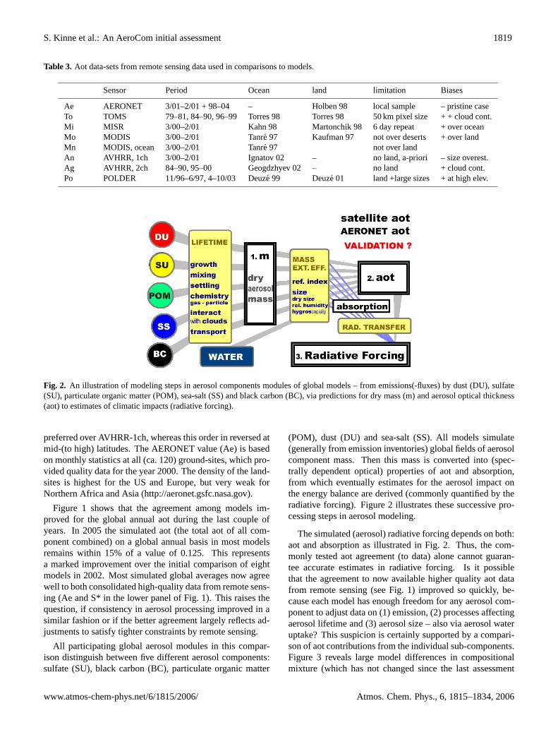
Figure 2. An illustration of modeling steps in aerosol components modules of global models – from emissions(-fluxes) by dust (DU), sulfate (SU), particulate organic matter (POM), sea-salt (SS) and black carbon (BC), via predictions for dry mass (m) and aerosol optical thickness (aot) to estimates of climatic impacts (radiative forcing).

The simulated (aerosol) radiative forcing depends on both: aot and absorption as illustrated in

Figure 2. Thus, the commonly tested aot agreement (to data) alone cannot guarantee accurate

estimates in radiative forcing. It is possible that the agreement to now available higher quality

aot data from remote sensing (see Figure 1) improved so quickly, because each model has

enough freedom for any aerosol component to adjust data on (1) emission, (2) processes

affecting aerosol lifetime and (3) aerosol size – also via aerosol water uptake? This suspicion is

certainly supported by a comparison of aot contributions from the individual sub-components.

Figure 3 reveals large model differences in compositional mixture (which has not changed

since the last assessment in Kinne et al. 2003). It also demonstrates that the agreement for the

sum of all components, which was presented in Figure 1 is a poor measure for overall model

skill and model diversity. Model diversity for each of the five component aot contributions

individually is significantly larger than for the combined total aot. This is also quantified in

Table 4, where annual global averages - on a component basis - are compared among all

aerosol modules. In the right-most column of Table 4, the diversity for just the 16 aerosol

Fig. 2. An illustration of modeling steps in aerosol components modules of global models – from emissions(-fluxes) by dust (DU), sulfate(SU), particulate organic matter (POM), sea-salt (SS) and black carbon (BC), via predictions for dry mass (m) and aerosol optical thickness(aot) to estimates of climatic impacts (radiative forcing).

preferred over AVHRR-1ch, whereas this order in reversed atmid-(to high) latitudes. The AERONET value (Ae) is basedon monthly statistics at all (ca. 120) ground-sites, which pro-vided quality data for the year 2000. The density of the land-sites is highest for the US and Europe, but very weak forNorthern Africa and Asia (http://aeronet.gsfc.nasa.gov).

Figure 1 shows that the agreement among models im-proved for the global annual aot during the last couple ofyears. In 2005 the simulated aot (the total aot of all com-ponent combined) on a global annual basis in most modelsremains within 15% of a value of 0.125. This representsa marked improvement over the initial comparison of eightmodels in 2002. Most simulated global averages now agreewell to both consolidated high-quality data from remote sens-ing (Ae and S* in the lower panel of Fig. 1). This raises thequestion, if consistency in aerosol processing improved in asimilar fashion or if the better agreement largely reflects ad-justments to satisfy tighter constraints by remote sensing.

All participating global aerosol modules in this compar-ison distinguish between five different aerosol components:sulfate (SU), black carbon (BC), particulate organic matter

(POM), dust (DU) and sea-salt (SS). All models simulate(generally from emission inventories) global fields of aerosolcomponent mass. Then this mass is converted into (spec-trally dependent optical) properties of aot and absorption,from which eventually estimates for the aerosol impact onthe energy balance are derived (commonly quantified by theradiative forcing). Figure 2 illustrates these successive pro-cessing steps in aerosol modeling.

The simulated (aerosol) radiative forcing depends on both:aot and absorption as illustrated in Fig. 2. Thus, the com-monly tested aot agreement (to data) alone cannot guaran-tee accurate estimates in radiative forcing. Is it possiblethat the agreement to now available higher quality aot datafrom remote sensing (see Fig. 1) improved so quickly, be-cause each model has enough freedom for any aerosol com-ponent to adjust data on (1) emission, (2) processes affectingaerosol lifetime and (3) aerosol size – also via aerosol wateruptake? This suspicion is certainly supported by a compari-son of aot contributions from the individual sub-components.Figure 3 reveals large model differences in compositionalmixture (which has not changed since the last assessment


http://aeronet.gsfc.nasa.gov


11

modules of the AeroCom exercise is summarized by total diversity (TD) and in brackets by

central diversity (CD): both TD and CD are defined by the ratio between the largest and

smallest average. Thus, a value of one corresponds to perfect agreement and any amount larger

than one is the adopted measure of diversity. TD refers to all models, whereas CD refers only

to the central 2/3 of all models - as extremes in modeling for CD are excluded.

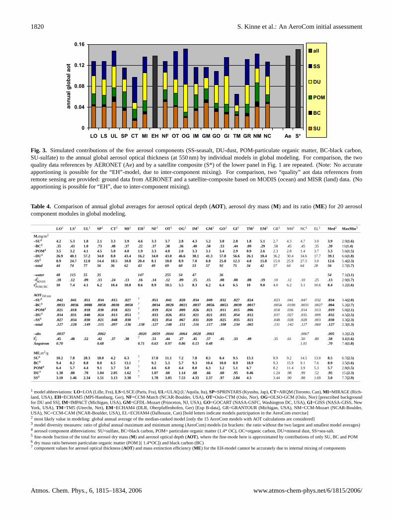
Figure 3. Individual contributions of the five aerosol components (SS-seasalt, DU-dust, POM-particulate organic matter, BC-black carbon, SU-sulfate) to the annual global aerosol optical thickness (at 550nm). For comparison, two ‘quality’ aot data references from remote sensing are provided: ground data from AERONET and a satellite-composite based on MODIS (ocean) and MISR (land) data. (No apportioning is possible for ‘EH’, due to inter-component mixing).

For aot, the CD of individual components contributions is between 2.0 and 2.7. This is three to

six times larger than for the component combined total of 1.3 (which was illustrated by model

comparison for 2005 in Figure 1). The largest component CDs for aot are associated with black

carbon, dust and sea-salt. CDs for aot-to-mass conversions (mass-extinction-efficiency)

indicate (see Table 4) that for sea-salt and dust differences in aerosol size are a major reason

for their aot diversity. Aerosol size is not only influenced by assumptions to primary emissions

but also by the permitted water uptake, which is controlled by assumptions to component

humidification and local ambient humidity. Table 4 indicates that on a global annual basis the

simulated aerosol water mass shows strong diversity and aerosol water mass is (at least)

comparable to the aerosol dry mass of all sub-components combined. Thus, for the hydrophilic

0

0.04

0.08

0.12

0.16

LO LS UL SP CT MI EH NF OT OG IM GM GO GI TM GR NM NC Ae S*

annu

al g

loba

l aot

all

SS

DU

POM

BC

SU

Fig. 3. Simulated contributions of the five aerosol components (SS-seasalt, DU-dust, POM-particulate organic matter, BC-black carbon,SU-sulfate) to the annual global aerosol optical thickness (at 550 nm) by individual models in global modeling. For comparison, the twoquality data references by AERONET (Ae) and by a satellite composite (S*) of the lower panel in Fig. 1 are repeated. (Note: No accurateapportioning is possible for the “EH”-model, due to inter-component mixing). For comparison, two “quality” aot data references fromremote sensing are provided: ground data from AERONET and a satellite-composite based on MODIS (ocean) and MISR (land) data. (Noapportioning is possible for “EH”, due to inter-component mixing).

Table 4. Comparison of annual global averages for aerosol optical depth (AOT ), aerosol dry mass (M ) and its ratio (ME ) for 20 aerosolcomponent modules in global modeling.

LO1 LS1 UL1 SP1 CT1 MI 1 EH1 NF1 OT1 OG1 IM 1 GM1 GO1 GI1 TM 1 EM1 GR1 NM1 NC1 EL1 Med2 MaxMin 3

M ,mg/m2

–SU4 4.2 5.3 1.8 2.1 3.3 3.9 4.6 3.3 3.7 2.8 4.3 5.2 3.8 2.8 1.8 5.12.7 4.3 4.7 3.0 3.9 2.9(1.6)–BC4 .35 .43 1.0 .73 .48 .37 .22 .37 .38 .36 .40 .50 .53 .44 .09 .29.58 .45 .45 .35 .39 11(1.4)–POM4 3.5 3.2 4.1 4.5 5.0 4.0 1.9 3.3 4.0 2.0 3.3 3.1 3.4 2.9 0.9 2.62.3 2.8 1.4 3.7 3.3 5.6(1.5)–DU4 26.9 40.1 57.2 34.0 8.8 43.4 16.2 34.0 43.0 46.6 38.1 41.3 57.8 56.6 26.1 18.436.2 30.4 34.6 17.7 39.1 6.6(1.8)-SS4 8.9 24.7 12.8 14.4 18.5 10.8 20.4 8.1 18.0 8.9 7.0 6.8 25.8 12.3 4.8 15.815.0 25.9 27.5 3.0 12.6 5.4(2.3)–total 44 74 77 56 36 62 43 49 69 60 53 57 92 75 34 42 57 64 64 28 56 2.7(1.7)

–water 48 115 55 35 147 255 54 47 36 54 7.1(3.1)–f5MASS .18 .12 .09 .13 .24 .13 .16 .14 .12 .09 .15 .15 .08 .08 .08 .19.10 .12 .10 .25 .13 2.9(1.7)r6POM/BC 10 7.4 4.1 6.2 10.4 10.8 8.6 8.9 10.5 5.5 8.3 6.2 6.4 6.5 10 9.04.0 6.2 3.1 10.6 8.4 3.2(1.6)

AOT550 nm–SU4 .042 .041 .051 .034 .015 .027 7 .051 .041 .020 .034 .049 .032 .027 .024 .023 .041 .047 .032 .034 3.4(2.0)–BC4 .0033 .0036 .0088 .0058 .0030 .00507 .0034 .0020 .0021 .0037 .0056 .0053 .0039 .0017 .0054 .0100 .0031 .0027 .004 5.2(2.7)–POM4 .021 .018 .018 .030 .018 .021 7 .019 .024 .009 .026 .021 .011 .015 .006 .018 .036 .014 .013 .019 5.0(2.1)–DU4 .034 .031 .040 .024 .013 .053 7 .033 .026 .053 .021 .021 .035 .054 .012 .037 .027 .035 .009 .032 4.5(2.5)–SS4 .027 .034 .030 .021 .048 .030 7 .021 .054 .067 .031 .020 .025 .035 .021 .048 .028 .028 .003 .030 3.3(2.3)–total .127 .128 .149 .115 .097 .136 .138 .127 .148 .151 .116 .117 .108 .134 .065 .131 .142 .127 .060 .127 2.3(1.3)

–abs .0037 .0062 .0020 .0059 .0044 .0064 .0028 .0061 .0067 .005 3.2(2.2)f5T

.45 .48 .52 .42 .37 .30 7 .51 .44 .27 .45 .57 .45 .33 .49 .35 .61 .50 .80 .50 3.1(1.6)Angstrom 0.70 0.68 0.71 0.63 0.97 0.86 0.13 0.48 1.01 .70 7.4(1.8)

ME ,m2/gSU4 10.2 7.8 28.3 18.0 4.2 6.3 7 17.8 11.1 7.2 7.8 8.5 8.4 9.5 13.3 8.9 9.2 14.5 13.0 8.5 6.7(2.5)BC4 9.4 8.2 8.8 8.0 6.5 13.1 7 9.2 5.3 5.7 9.3 10.4 10.0 8.9 18.9 9.3 15.9 9.1 7.6 8.9 3.5(1.6)POM4 6.4 5.7 4.4 9.1 3.7 5.0 7 4.6 6.0 4.4 8.0 6.3 3.2 5.1 6.7 8.2 11.4 3.9 5.3 5.7 2.8(1.5)DU4 1.38 .88 .70 1.04 2.05 1.62 7 1.07 .60 1.14 .68 .66 .60 .95 0.46 1.24 .98 .99 .52 .95 15.(2.3)SS4 3.10 1.46 2.34 1.51 3.13 3.38 7 1.78 3.05 7.53 4.33 2.37 .97 2.84 4.3 3.44 .90 .88 1.69 3.0 7.7(2.9)

1 model abbreviations:LO=LOA (Lille, Fra),LS=LSCE (Paris, Fra),UL=ULAQ (L’Aquila, Ita), SP=SPRINTARS (Kyushu, Jap),CT=ARQM (Toronto, Can),MI =MIRAGE (Rich-land, USA),EH=ECHAM5 (MPI-Hamburg, Ger),NF=CCM-Match (NCAR-Boulder, USA),OT=Oslo-CTM (Oslo, Nor),OG=OLSO-GCM (Oslo, Nor) [prescribed backgroundfor DU and SS],IM =IMPACT (Michigan, USA),GM=GFDL-Mozart (Princeton, NJ, USA),GO=GOCART (NASA-GSFC, Washington DC, USA),GI=GISS (NASA-GISS, NewYork, USA), TM =TM5 (Utrecht, Net),EM=ECHAM4 (DLR, Oberpfaffenhofen, Ger) [Exp B-data], GR=GRANTOUR (Michigan, USA), NM=CCM-Mozart (NCAR-Boulder,USA), NC=CCM-CAM (NCAR-Boulder, USA), EL=ECHAM4 (Dalhousie, Can) [bold letters indicate models participation in the AeroCom exercise]2 most likely value in modeling: global annual average of the median-ranked model [only the 15 AeroCom models with AOT calculations are considered]3 model diversity measures: ratio of global annual maximum and minimum among (AeroCom) models (in brackets: the ratio without the two largest and smallest model averages)4 aerosol component abbreviations: SU=sulfate, BC=black carbon, POM= particulate organic matter (1.4* OC), OC=organic carbon, DU=mineral dust, SS=sea-salt.5 fine-mode fraction of the total for aerosol dry mass (M ) and aerosol optical depth (AOT ), where the fine-mode here is approximated by contributions of only SU, BC and POM6 dry mass ratio between particulate organic matter (POM [( 1.4*OC]) and black carbon (BC)7 component values for aerosol optical thickness (AOT ) and mass extinction efficiency (ME ) for the EH-model cannot be accurately due to internal mixing of components



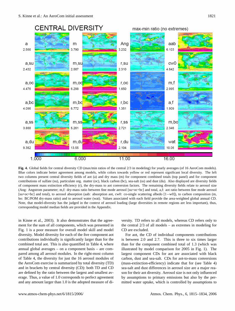
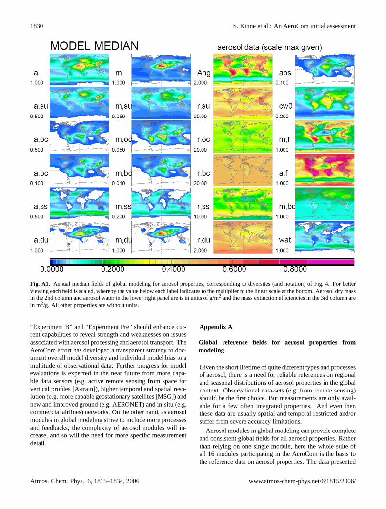
Fig. 4. Global fields for central diversity CD (max/min ratios of the central 2/3 in modeling) for yearly averages (of 16 AeroCom models).Blue colors indicate better agreement among models, while colors towards yellow or red represent significant local diversity. The lefttwo columns present central diversity fields of aot (a) and dry mass (m) for component combined totals (top panel) and for componentcontributions of sulfate (su), particulate org. matter (oc), black carbon (bc), sea-salt (ss) and dust (du). Also displayed are diversity fieldsof component mass extinction efficiency (r), the dry-mass to aot conversion factors. The remaining diversity fields relate to aerosol size(Ang: Angstrom parameter; m,f: dry-mass ratio between fine mode aerosol [su+oc+bc] and total, a,f: aot ratio between fine mode aerosol[su+oc+bc] and total), to aerosol absorption (aab: absorption aot, cw0: co-single scattering albedo [1−w0]), to carbon composition (m,bo: BC/POM dry-mass ratio) and to aerosol water (wat). Values associated with each field provide the area-weighted global annual CD.Note, that model-diversity has the judged in the context of aerosol loading (large diversities in remote regions are less important), thus,corresponding model median fields are provided in the Appendix.

in Kinne et al., 2003). It also demonstrates that the agree-ment for the sum of all components, which was presented inFig. 1 is a poor measure for overall model skill and modeldiversity. Model diversity for each of the five component aotcontributions individually is significantly larger than for thecombined total aot. This is also quantified in Table 4, whereannual global averages – on a component basis – are com-pared among all aerosol modules. In the right-most columnof Table 4, the diversity for just the 16 aerosol modules ofthe AeroCom exercise is summarized by total diversity (TD)and in brackets by central diversity (CD): both TD and CDare defined by the ratio between the largest and smallest av-erage. Thus, a value of 1.0 corresponds to perfect agreementand any amount larger than 1.0 is the adopted measure of di-

versity. TD refers to all models, whereas CD refers only tothe central 2/3 of all models – as extremes in modeling forCD are excluded.

For aot, the CD of individual components contributionsis between 2.0 and 2.7. This is three to six times largerthan for the component combined total of 1.3 (which wasillustrated by model comparison for 2005 in Fig. 1). Thelargest component CDs for aot are associated with blackcarbon, dust and sea-salt. CDs for aot-to-mass conversions(mass-extinction-efficiency) indicate that for (see Table 4)sea-salt and dust differences in aerosol size are a major rea-son for their aot diversity. Aerosol size is not only influencedby assumptions to primary emissions but also by the per-mitted water uptake, which is controlled by assumptions to



component humidification and local ambient humidity. Ta-ble 4 indicates that on a global annual basis the simulatedaerosol water mass shows strong diversity and aerosol watermass is (at least) comparable to the aerosol dry mass of allsub-components combined. Thus, for the hydrophilic com-ponents of sea-salt and sulfate larger model diversities foraot than for dry mass are expected. For global sea-salt CDs,however, this trend is reversed. A possible explanation is thetransport of larger sea salt particles in some models, whichcreates larger diversity near sources, more so for mass thanfor aot. A contributing factor is also the large sea-salt massdiversity over continents (see discussions in the next sectionand the presentation of diversity fields in Fig. 4). This illus-trates that even regions with significant lower concentrationscan distort the global average and that the reliance on globalaverages can be misleading. Thus, local diversity fields areexplored next.

3.2 Annual fields

Given the short-lived nature of aerosol, evaluations at suf-ficient resolution in time and space will allow more usefulinsights into issues of aerosol global modeling. To extendthe model diversity assessments of Table 4, local CDs for24 annual fields are presented in Fig. 4. All models wereinterpolated to the same horizontal resolution of 1◦

×1◦ lat-itude/longitude. At each grid point all models were rankedaccording to the simulated magnitude into a probability dis-tribution function (PDF). The ratio between the 83% and the17% values of the PDF (such that extremes in modeling areignored) define the CDs in Fig. 4. It can be seen that modeldiversity usually increases towards remote regions, largelydue to differences in transport and/or aerosol processing (e.g.removal). However, diversity has to be judged also in thecontext of the absolute concentration, as larger diversitiesare less meaningful in regions of overall low concentrations.Global fields of the model median (the 50% value of thePDF) are presented in figures of the Appendix, where Fig. A1corresponds to Fig. 4.

Model diversity is usually larger over land than overoceans for total dry mass and total aot. The largest differ-ences occur in central Asia and extend eastwards to westernregions of North America. Sub-component diversity is usu-ally stronger, but component diversity patterns differ. Forsulfate the diversity for aot is increased over mass diversityat low latitude land regions and in the continental outflow re-gions. Large model diversity for aerosol water may providean explanation. For organic and black carbon the diversitiesare usually larger than for sulfate. Particular large are car-bon diversities over some oceanic regions. This location overthe ocean for the rather insoluble organic particles suggestsmodel differences in transport and removal processes whichaffect the transport to remote regions. As differences in trans-port strongly contribute to model diversity, it does not sur-prise that for dust, whose global distributions are largely de-

fined by transport, display larger diversities away from dustsource regions. The fact that dust diversity (and sea-salt di-versity over oceans) for aot is significantly smaller than formass could indicate deliberate choices for size with the goalto match expectations. However, it should be pointed out,that different cut-off assumptions for the largest dust and sea-salt sizes create mechanically larger diversity for mass thanfor aot because the largest particles contribute a lot to massbut little to aot. The size-diversity for dust and sea-salt is alsodemonstrated in larger diversities for mass-to-aot conversionfactors (the r-panels in the third column of Fig. 4), comparedto carbon or sulfate species. Also, the largest model diversityfor aerosol size, illustrated via the Angstrom parameter (label“Ang”), occurs in regions, where dust (Northern Africa andAsia) and sea-salt (southern mid-latitudes) are the dominantcomponents.

A comparison of the panels in the upper corners of Fig. 4between aerosol optical depth (label “a”) and its fraction as-sociated with absorption (label “aab”) illustrates that diver-sity for aerosol absorption is significantly larger than diver-sity for aerosol optical thickness. This indicates that reduceduncertainties in aerosol direct forcing require primarily im-provements to the characterization of the local (or regional)aerosol composition. Larger diversities for absorption occurtowards remote regions. This suggests that aerosol process-ing during long-range transport is a key issue for reductionsof model diversity. Emissions which dominate the diversitynear the sources over land seem to be more homogeneousin models, probably because similar emission inventories areused by different modeling groups.

3.3 Comparisons to observational data

Although model diversity is of interest, it is not necessarily ameasure of the real uncertainty. Similar assumptions or ap-proaches in modeling can overshadow real uncertainties, asfor example in the case of moderate diversity found for par-ticulate organic matter (organic carbon mass) despite largeuncertainties for its emission factors, secondary production,humidification and absorption.

Model diversity is of limited value without quality ref-erence observations, which from now on is referred to asdata, for simplicity. Unfortunately, reference data are onlyavailable for a few (and often integrated) properties. Andeven if data exist, they usually suffer from limitations to (of-ten poorly defined) accuracy and from restrictions of spatialand/or temporal nature. Subsequent comparisons focus ontwo properties that are critical in the context of aerosol radia-tive forcing: mid-visible values for aerosol optical thickness(aot) and its fraction linked absorption, the aerosol absorp-tion optical thickness (aab). Two data references based onyear 2000 measurements were adopted.

The first data (local) reference is provided by quality as-sured data of sun-/sky-photometer robots distributed all overthe world as part of the AERONET network (Holben et al.,



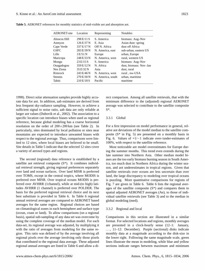
Table 5. AERONET references for monthly statistics of mid-visible aot and absorption aot.

AERONET-site Location Representing Notables

Abracos Hill 298 E/11 S S. America biomass: Aug–NovAnmyon 126 E/37 N E. Asia Asian dust: springCape Verde 337 E/17 N Off N. Africa dust off AfricaGSFC 283 E/39 N N. America, east sub-urban, eastern USLille 3 E/51 N Europe urban, EuropeMaricopa 248 E/33 N N. America, west rural, western USMongu 23 E/15 S S. America biomass: Aug–NovOuagadogou 359 E/12 N N. Africa dust, biomass: Nov–JanNes Ziona 35 E/32 N Asia dust, ruralRimrock 243 E/46 N N. America, west rural , nw-USAStennis 270 E/30 N N. America, south urban, maritimeTahiti 210 E/18 S Pacific maritime

1998). Direct solar attenuation samples provide highly accu-rate data for aot. In addition, aab estimates are derived fromless frequent sky-radiance sampling. However, to achieve asufficient signal to noise ratio, aab data are only reliable atlarger aot values (Dubovik et al., 2002). The association to aspecific location can introduce biases when used as regionalreference, because global modeling has a coarse horizontalresolution on the order of 200×200 km (see Table 2). Inparticularly, sites dominated by local pollution or sites nearmountains are expected to introduce unwanted biases withrespect to the regional average. Thus, comparisons were lim-ited to 12 sites, where local biases are believed to be small.Site details in Table 5 indicate that the selected 12 sites covera variety of aerosol types and regions.

The second (regional) data reference is established by asatellite aot retrieval composite (S*). It combines individ-ual retrieval strength, giving regional preferences separatelyover land and ocean surfaces. Over land MISR is preferredover TOMS, except in the central tropics, where MODIS ispreferred over MISR. Over tropical oceans MODIS is pre-ferred over AVHRR (1channel), while at mid-(to high) lati-tudes AVHRR (1 channel) is preferred over POLDER. Thebasis for the preferred regional retrieval choice and its nextbest substitute is provided in Table 6. In Table 6 regionalannual retrieval averages are compared to AERONET basedaverages for the same region. Regional choices are basedon climatological zones in each hemisphere and surface type(ocean, coast or land). To allow comparisons (on a regionalbasis), spatial sub-sampling of any data set was overcome byusing the complete coverage of the median model. For eachdata-set, its regional average was adjusted, by multiplying itwith the ratio of averages from modeling for the same re-gion. This ratio was defined of by the average involving allregional pixels over the average involving only those pixelsthat contributed to the regional data average. These adjustedregional annual averages are listed in Table 6 and allow a di-

rect comparison. Among all satellite retrievals, that with theminimum difference to the (adjusted) regional AERONETaverage was selected to contribute to the satellite compositeS*.

3.3.1 Global

For a first impression on model performance in general, rel-ative aot deviations of the model median to the satellite com-posite (S* in Fig. 5) are presented on a monthly basis inFig. 6. Values of +1/−1 indicate over-/under-estimates of100%, with respect to the satellite reference.

Most noticeable are model overestimates for Europe dur-ing the summer months. This trend even extends during thelate summer into Northern Asia. Other median model bi-ases are the too early biomass burning season in South Amer-ica, too much dust in Northern Africa during the winter sea-son, and aot underestimates in tropical regions. Given thatsatellite retrievals over oceans are less uncertain than overland, the large discrepancy to modeling over tropical oceansis puzzling. More quantitative comparisons for regions ofFig. 7 are given in Table 6. Table 6 lists the regional aver-ages of the satellite composite (S*) and compares them tospatial adjusted AERONET averages (Ae), to those of indi-vidual satellite retrievals (see Table 3) and to the median inglobal modeling (med).

3.3.2 Regional and local

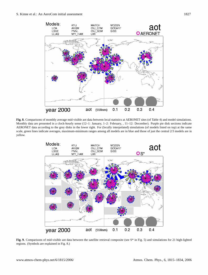
Comparisons in this section are illustrated in a similarformat. For selected locations and regions, monthly averagesare presented in a clock-hourly sense (12–1: January,. . . , 11–12: December). Purple (sectional) disks indicatemonthly data at a magnitude according to the disk-size inthe lower right. Following the same magnitude scale, greenlines illustrate the mean in modeling, while blue and yellowsections indicate ranges between maximum and minimum



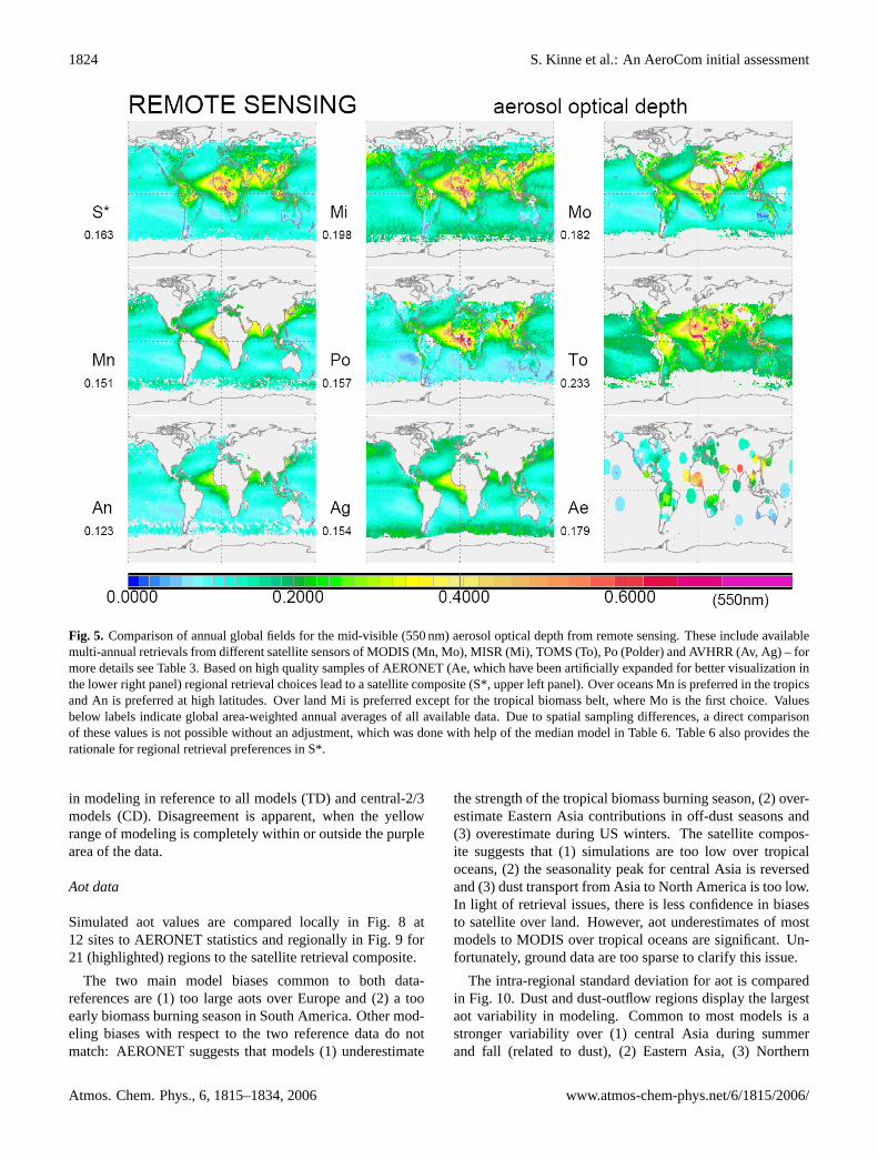
Fig. 5. Comparison of annual global fields for the mid-visible (550 nm) aerosol optical depth from remote sensing. These include availablemulti-annual retrievals from different satellite sensors of MODIS (Mn, Mo), MISR (Mi), TOMS (To), Po (Polder) and AVHRR (Av, Ag) – formore details see Table 3. Based on high quality samples of AERONET (Ae, which have been artificially expanded for better visualization inthe lower right panel) regional retrieval choices lead to a satellite composite (S*, upper left panel). Over oceans Mn is preferred in the tropicsand An is preferred at high latitudes. Over land Mi is preferred except for the tropical biomass belt, where Mo is the first choice. Valuesbelow labels indicate global area-weighted annual averages of all available data. Due to spatial sampling differences, a direct comparisonof these values is not possible without an adjustment, which was done with help of the median model in Table 6. Table 6 also provides therationale for regional retrieval preferences in S*.

in modeling in reference to all models (TD) and central-2/3models (CD). Disagreement is apparent, when the yellowrange of modeling is completely within or outside the purplearea of the data.

Aot data

Simulated aot values are compared locally in Fig. 8 at12 sites to AERONET statistics and regionally in Fig. 9 for21 (highlighted) regions to the satellite retrieval composite.

The two main model biases common to both data-references are (1) too large aots over Europe and (2) a tooearly biomass burning season in South America. Other mod-eling biases with respect to the two reference data do notmatch: AERONET suggests that models (1) underestimate

the strength of the tropical biomass burning season, (2) over-estimate Eastern Asia contributions in off-dust seasons and(3) overestimate during US winters. The satellite compos-ite suggests that (1) simulations are too low over tropicaloceans, (2) the seasonality peak for central Asia is reversedand (3) dust transport from Asia to North America is too low.In light of retrieval issues, there is less confidence in biasesto satellite over land. However, aot underestimates of mostmodels to MODIS over tropical oceans are significant. Un-fortunately, ground data are too sparse to clarify this issue.

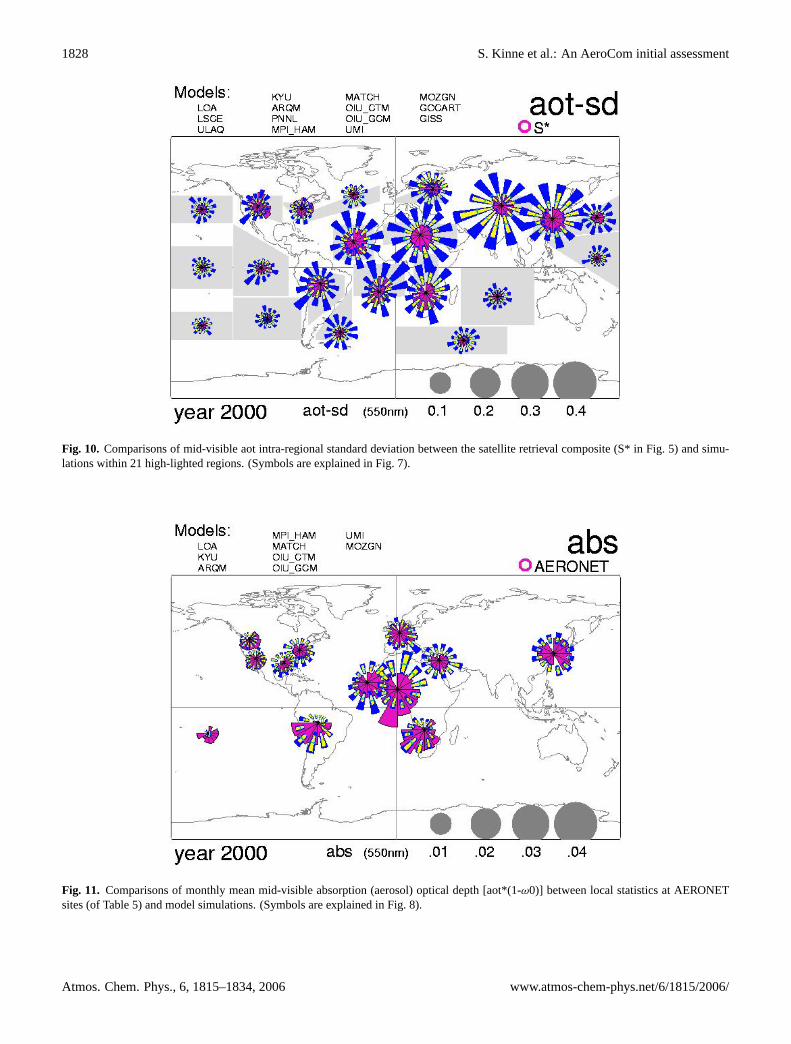
The intra-regional standard deviation for aot is comparedin Fig. 10. Dust and dust-outflow regions display the largestaot variability in modeling. Common to most models is astronger variability over (1) central Asia during summerand fall (related to dust), (2) Eastern Asia, (3) Northern



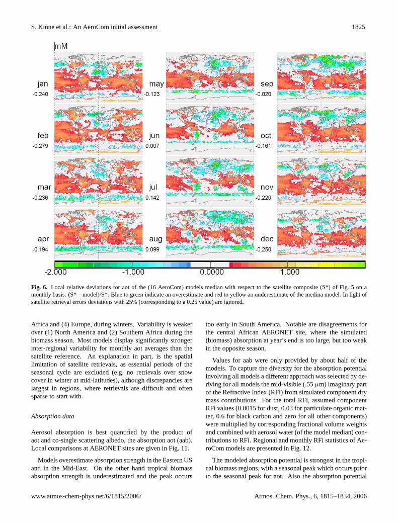
Fig. 6. Local relative deviations for aot of the (16 AeroCom) models median with respect to the satellite composite (S*) of Fig. 5 on amonthly basis: (S* – model)/S*. Blue to green indicate an overestimate and red to yellow an underestimate of the medina model. In light ofsatellite retrieval errors deviations with 25% (corresponding to a 0.25 value) are ignored.

Africa and (4) Europe, during winters. Variability is weakerover (1) North America and (2) Southern Africa during thebiomass season. Most models display significantly strongerinter-regional variability for monthly aot averages than thesatellite reference. An explanation in part, is the spatiallimitation of satellite retrievals, as essential periods of theseasonal cycle are excluded (e.g. no retrievals over snowcover in winter at mid-latitudes), although discrepancies arelargest in regions, where retrievals are difficult and oftensparse to start with.

Absorption data

Aerosol absorption is best quantified by the product ofaot and co-single scattering albedo, the absorption aot (aab).Local comparisons at AERONET sites are given in Fig. 11.

Models overestimate absorption strength in the Eastern USand in the Mid-East. On the other hand tropical biomassabsorption strength is underestimated and the peak occurs

too early in South America. Notable are disagreements forthe central African AERONET site, where the simulated(biomass) absorption at year’s end is too large, but too weakin the opposite season.

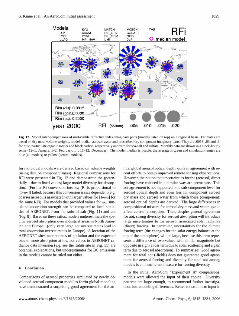
Values for aab were only provided by about half of themodels. To capture the diversity for the absorption potentialinvolving all models a different approach was selected by de-riving for all models the mid-visible (.55µm) imaginary partof the Refractive Index (RFi) from simulated component drymass contributions. For the total RFi, assumed componentRFi values (0.0015 for dust, 0.03 for particulate organic mat-ter, 0.6 for black carbon and zero for all other components)were multiplied by corresponding fractional volume weightsand combined with aerosol water (of the model median) con-tributions to RFi. Regional and monthly RFi statistics of Ae-roCom models are presented in Fig. 12.

The modeled absorption potential is strongest in the tropi-cal biomass regions, with a seasonal peak which occurs priorto the seasonal peak for aot. Also the absorption potential



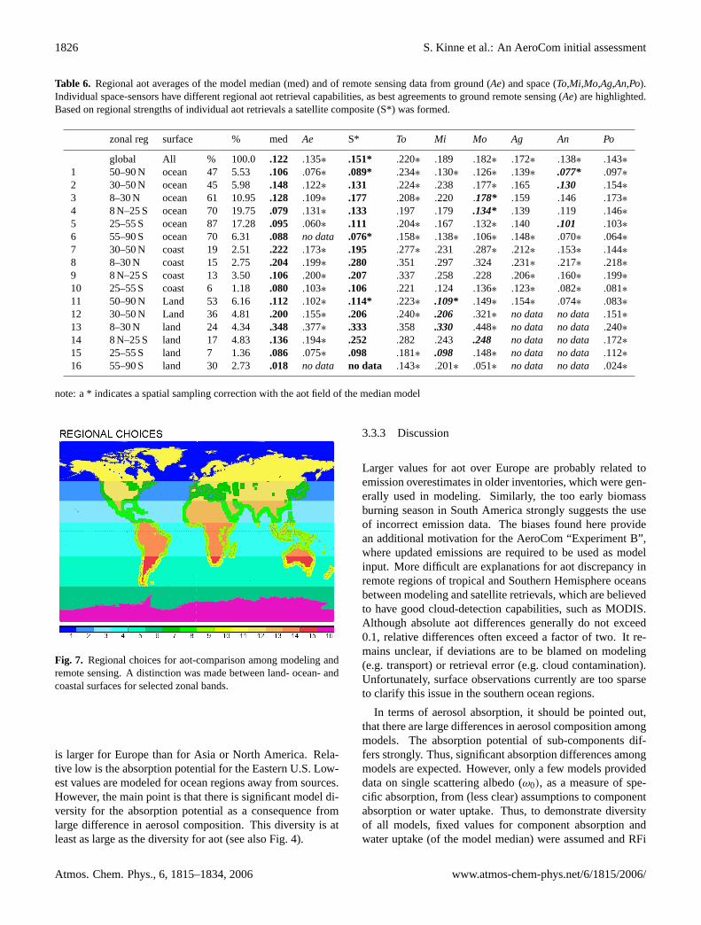
Table 6. Regional aot averages of the model median (med) and of remote sensing data from ground (Ae) and space (To,Mi,Mo,Ag,An,Po).Individual space-sensors have different regional aot retrieval capabilities, as best agreements to ground remote sensing (Ae) are highlighted.Based on regional strengths of individual aot retrievals a satellite composite (S*) was formed.

zonal reg surface % med Ae S* To Mi Mo Ag An Po

global All % 100.0 .122 .135∗ .151* .220∗ .189 .182∗ .172∗ .138∗ .143∗1 50–90 N ocean 47 5.53 .106 .076∗ .089* .234∗ .130∗ .126∗ .139∗ .077* .097∗2 30–50 N ocean 45 5.98 .148 .122∗ .131 .224∗ .238 .177∗ .165 .130 .154∗3 8–30 N ocean 61 10.95 .128 .109∗ .177 .208∗ .220 .178* .159 .146 .173∗4 8 N–25 S ocean 70 19.75 .079 .131∗ .133 .197 .179 .134* .139 .119 .146∗5 25–55 S ocean 87 17.28 .095 .060∗ .111 .204∗ .167 .132∗ .140 .101 .103∗6 55–90 S ocean 70 6.31 .088 no data .076* .158∗ .138∗ .106∗ .148∗ .070∗ .064∗7 30–50 N coast 19 2.51 .222 .173∗ .195 .277∗ .231 .287∗ .212∗ .153∗ .144∗8 8–30 N coast 15 2.75 .204 .199∗ .280 .351 .297 .324 .231∗ .217∗ .218∗9 8 N–25 S coast 13 3.50 .106 .200∗ .207 .337 .258 .228 .206∗ .160∗ .199∗10 25–55 S coast 6 1.18 .080 .103∗ .106 .221 .124 .136∗ .123∗ .082∗ .081∗11 50–90 N Land 53 6.16 .112 .102∗ .114* .223∗ .109* .149∗ .154∗ .074∗ .083∗12 30–50 N Land 36 4.81 .200 .155∗ .206 .240∗ .206 .321∗ no data no data .151∗13 8–30 N land 24 4.34 .348 .377∗ .333 .358 .330 .448∗ no data no data .240∗14 8 N–25 S land 17 4.83 .136 .194∗ .252 .282 .243 .248 no data no data .172∗15 25–55 S land 7 1.36 .086 .075∗ .098 .181∗ .098 .148∗ no data no data .112∗16 55–90 S land 30 2.73 .018 no data no data .143∗ .201∗ .051∗ no data no data .024∗

note: a * indicates a spatial sampling correction with the aot field of the median model

Fig. 7. Regional choices for aot-comparison among modeling andremote sensing. A distinction was made between land- ocean- andcoastal surfaces for selected zonal bands.

is larger for Europe than for Asia or North America. Rela-tive low is the absorption potential for the Eastern U.S. Low-est values are modeled for ocean regions away from sources.However, the main point is that there is significant model di-versity for the absorption potential as a consequence fromlarge difference in aerosol composition. This diversity is atleast as large as the diversity for aot (see also Fig. 4).

3.3.3 Discussion

Larger values for aot over Europe are probably related toemission overestimates in older inventories, which were gen-erally used in modeling. Similarly, the too early biomassburning season in South America strongly suggests the useof incorrect emission data. The biases found here providean additional motivation for the AeroCom “Experiment B”,where updated emissions are required to be used as modelinput. More difficult are explanations for aot discrepancy inremote regions of tropical and Southern Hemisphere oceansbetween modeling and satellite retrievals, which are believedto have good cloud-detection capabilities, such as MODIS.Although absolute aot differences generally do not exceed0.1, relative differences often exceed a factor of two. It re-mains unclear, if deviations are to be blamed on modeling(e.g. transport) or retrieval error (e.g. cloud contamination).Unfortunately, surface observations currently are too sparseto clarify this issue in the southern ocean regions.

In terms of aerosol absorption, it should be pointed out,that there are large differences in aerosol composition amongmodels. The absorption potential of sub-components dif-fers strongly. Thus, significant absorption differences amongmodels are expected. However, only a few models provideddata on single scattering albedo (ω0), as a measure of spe-cific absorption, from (less clear) assumptions to componentabsorption or water uptake. Thus, to demonstrate diversityof all models, fixed values for component absorption andwater uptake (of the model median) were assumed and RFi



21

Simulated aot data are compared locally in Figure 8 at 12 sites to AERONET statistics and

regionally in Figure 9 for 21 (highlighted) regions to the satellite retrieval composite.

Figure 8: Comparisons of monthly average mid-visible aot data between local statistics at AERONET sites (of Table 4) and model simulations. Monthly data are presented in a clock-hourly sense (12-1: Jan, 1-2: Feb, , 11-12: Dec). Purple pie disk sections indicate AERONET data according to the grey disks in the lower right. For (locally interpolated) simulations (of models listed on top) at the same scale, green lines indicate averages, maximum-minimum ranges among all models are in blue and those of just the central 2/3 models are in yellow.

The two main model biases common to both data-references are (1) too large aots over Europe

and (2) a too early biomass burning season in South America. Other modeling biases with

respect to the two reference data do not match: AERONET suggests that models (1)

underestimate the strength of the tropical biomass burning season, (2) overestimate Eastern

Asia contributions in off-dust seasons and (3) overestimate during US winters. The satellite

composite suggests that (1) simulations are too low over tropical oceans, (2) the seasonality

peak for central Asia is reversed and (3) dust transport from Asia to North America is too low.

In light of retrieval issues, there is less confidence in biases to satellite over land. However, aot

Fig. 8. Comparisons of monthly average mid-visible aot data between local statistics at AERONET sites (of Table 4) and model simulations.Monthly data are presented in a clock-hourly sense (12–1: January, 1–2: February, , 11–12: December). Purple pie disk sections indicateAERONET data according to the grey disks in the lower right. For (locally interpolated) simulations (of models listed on top) at the samescale, green lines indicate averages, maximum-minimum ranges among all models are in blue and those of just the central 2/3 models are inyellow.

22

underestimates of most models to MODIS over tropical oceans are significant. Unfortunately,

ground data are too spare to clarify this issue.

Figure 9: Comparisons of mid-visible aot data between the satellite retrieval composite (see S* in Figure 5) and simulations for 21 high-lighted regions. (Symbols are explained in Figure 8.)

The intra-regional standard deviation for aot is compared in Figure 10. Dust and dust-outflow

regions display the largest aot variability in modeling. Common to most models is a stronger

variability over (1) central Asia during summer and fall (related to dust), (2) Eastern Asia, (3)

Northern Africa and (4) Europe, during winters. Variability is weaker over (1) North America

and (2) Southern Africa during the biomass season. Most models display significantly stronger

inter-regional variability for monthly aot averages than the satellite reference, although

discrepancies are largest in regions, where retrievals are difficult and often sparse to start with.

Fig. 9. Comparisons of mid-visible aot data between the satellite retrieval composite (see S* in Fig. 5) and simulations for 21 high-lightedregions. (Symbols are explained in Fig. 8.)



23

Figure 10: Comparisons of mid-visible aot intra-regional standard deviation between the satellite retrieval composite (S* in Figure 5) and simulations within 21 high-lighted regions. (Symbols are explained in Figure 7).

3.3.2.2. absorption data

Aerosol absorption is best quantified by the product of aot and co-single scattering albedo, the

absorption aot (aab). Local comparisons at AERONET sites are given in Figure 11.

Fig. 10. Comparisons of mid-visible aot intra-regional standard deviation between the satellite retrieval composite (S* in Fig. 5) and simu-lations within 21 high-lighted regions. (Symbols are explained in Fig. 7).

24

Figure 11: Comparisons of monthly mean mid-visible absorption (aerosol) optical depth [aot*(1-ω0)] between local statistics at AERONET sites (of Table 5) and model simulations. (Symbols are explained in Figure 8).

Models overestimate absorption strength in the Eastern US and in the Mid-East. On the other

hand tropical biomass absorption strength is underestimated and the peak occurs too early in

South America. Notable are disagreements for the central African AERONET site, where the

simulated (biomass) absorption at year’s end is too large, but too weak in the opposite season.

Values for aab were only provided by about half of the models. To capture the diversity for the

absorption potential involving all models a different approach was selected by deriving for all

models the mid-visible (.55µm) imaginary part of the Refractive Index (RFi) from simulated

component dry mass contributions. For the total RFi, assumed component RFi values (0.0015

for dust, 0.03 for particulate organic matter, 0.6 for black carbon and zero for all other

components) were multiplied by corresponding fractional volume weights and combined with

aerosol water (of the model median) contributions to RFi. Regional and monthly RFi statistics

of AeroCom models are presented in Figure 12.

Fig. 11. Comparisons of monthly mean mid-visible absorption (aerosol) optical depth [aot*(1-ω0)] between local statistics at AERONETsites (of Table 5) and model simulations. (Symbols are explained in Fig. 8).



25

Figure 12: Model inter-comparisons of mid-visible refractive index imaginary parts (models listed on top) on a regional basis. Estimates are based on dry mass volume weights, model median aerosol water and prescribed dry component imaginary parts: They are .0015, .03 and .6, for dust, particulate organic matter and black carbon, respectively and zero for sea-salt and sulfate. Monthly data are shown in a clock-hourly sense (12-1: Jan, 1-2: Feb, …, 11-12: Dec). The model median is purple, the average is green and simulation-ranges are blue (all models) or yellow (central models).

The modeled absorption potential is strongest in the tropical biomass regions, with a seasonal

peak which occurs prior to the seasonal peak for aot. Also the absorption potential is larger for

Europe than for Asia or North America. Relative low is the absorption potential for the Eastern

US. Lowest values are modeled for ocean regions away from sources. However, the main point

is that there is significant model diversity for the absorption potential as a consequence from

large difference in aerosol composition. This diversity is at least as large as the diversity for aot

(see also Figure 4).

Fig. 12. Model inter-comparisons of mid-visible refractive index imaginary parts (models listed on top) on a regional basis. Estimates arebased on dry mass volume weights, model median aerosol water and prescribed dry component imaginary parts: They are .0015, .03 and .6,for dust, particulate organic matter and black carbon, respectively and zero for sea-salt and sulfate. Monthly data are shown in a clock-hourlysense (12–1: January, 1–2: February, . . . , 11–12: December). The model median is purple, the average is green and simulation-ranges areblue (all models) or yellow (central models).

for individual models were derived based on volume weights(using data on component mass). Regional comparisons forRFi were presented in Fig. 12 and demonstrate the (poten-tially – due to fixed values) large model diversity for absorp-tion. (Further Ri conversion intoω0 (Ri is proportional to[1–ω0]) failed, because this conversion is size dependent (e.g.coarser aerosol is associated with larger values for [1–ω0] forthe same RFi). For models that provided values forω0, sim-ulated absorption strength can be compared to local statis-tics of AERONET, from the ratio of aab (Fig. 11) and aot(Fig. 8). Based on these ratios, models underestimate the spe-cific aerosol absorption over industrial areas in North Amer-ica and Europe. (only very large aot overestimates lead tototal absorption overestimates in Europe). A location of theAERONET sites near sources of pollution and the expectedbias to more absorption at low aot values in AERONET ra-diance data inversion (e.g. see the Tahiti site in Fig. 11) arepotential explanations, but underestimates for BC emissionsin the models cannot be ruled out either.

4 Conclusion

Comparisons of aerosol properties simulated by newly de-veloped aerosol component modules for/in global modelinghave demonstrated a surprising good agreement for the an-

nual global aerosol optical depth, quite in agreement with re-cent efforts to obtain improved remote sensing observations.However, the notion that uncertainties for the (aerosol) directforcing have reduced in a similar way are premature. Thisaot agreement is not supported on a sub-component level foraerosol optical depth and even less for component aerosoldry mass and aerosol water from which these (component)aerosol optical depths are derived. The large differences incompositional mixture for aerosol dry mass and water uptakeaffect aerosol absorption. Thus, despite general agreementfor aot, strong diversity for aerosol absorption will introducelarge uncertainties to the aerosol associated solar radiative(direct) forcing. In particular, uncertainties for the climateforcing term (the changes for the solar energy balance at thetop of the atmosphere) will be large, because this term repre-sents a difference of two values with similar magnitude butopposite in sign (a loss term due to solar scattering and a gainterm due to aerosol absorption). To summarize: Good agree-ment for total aot (-fields) does not guarantee good agree-ment for aerosol forcing and diversity for total aot amongmodels is an insufficient measure for forcing diversity.

In the initial AeroCom “Experiment A” comparisons,models were allowed the input of their choice. Diversitypatterns are large enough, to recommend further investiga-tions into modeling differences. Better constraints to input in



Fig. A1. Annual median fields of global modeling for aerosol properties, corresponding to diversites (and notation) of Fig. 4. For betterviewing each field is scaled, whereby the value below each label indicates to the multiplier to the linear scale at the bottom. Aerosol dry massin the 2nd column and aerosol water in the lower right panel are is in units of g/m2 and the mass extinction efficiencies in the 3rd column arein m2/g. All other properties are without units.

“Experiment B” and “Experiment Pre” should enhance cur-rent capabilities to reveal strength and weaknesses on issuesassociated with aerosol processing and aerosol transport. TheAeroCom effort has developed a transparent strategy to doc-ument overall model diversity and individual model bias to amultitude of observational data. Further progress for modelevaluations is expected in the near future from more capa-ble data sensors (e.g. active remote sensing from space forvertical profiles [A-train]), higher temporal and spatial reso-lution (e.g. more capable geostationary satellites [MSG]) andnew and improved ground (e.g. AERONET) and in-situ (e.g.commercial airlines) networks. On the other hand, as aerosolmodules in global modeling strive to include more processesand feedbacks, the complexity of aerosol modules will in-crease, and so will the need for more specific measurementdetail.

Appendix A

Global reference fields for aerosol properties frommodeling

Given the short lifetime of quite different types and processesof aerosol, there is a need for reliable references on regionaland seasonal distributions of aerosol properties in the globalcontext. Observational data-sets (e.g. from remote sensing)should be the first choice. But measurements are only avail-able for a few often integrated properties. And even thenthese data are usually spatial and temporal restricted and/orsuffer from severe accuracy limitations.

Aerosol modules in global modeling can provide completeand consistent global fields for all aerosol properties. Ratherthan relying on one single module, here the whole suite ofall 16 modules participating in the AeroCom is the basis tothe reference data on aerosol properties. The data presented



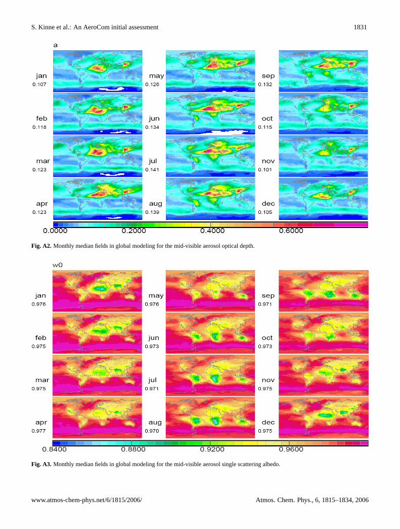
Fig. A2. Monthly median fields in global modeling for the mid-visible aerosol optical depth.

Fig. A3. Monthly median fields in global modeling for the mid-visible aerosol single scattering albedo.



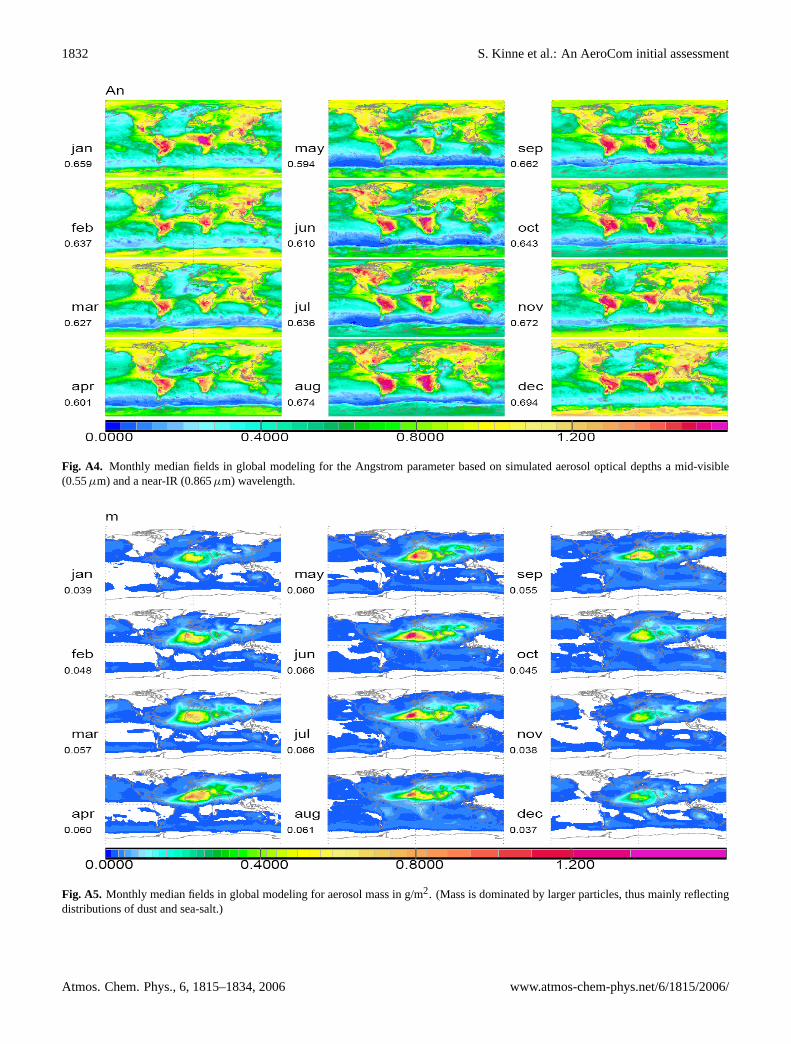
Fig. A4. Monthly median fields in global modeling for the Angstrom parameter based on simulated aerosol optical depths a mid-visible(0.55µm) and a near-IR (0.865µm) wavelength.

Fig. A5. Monthly median fields in global modeling for aerosol mass in g/m2. (Mass is dominated by larger particles, thus mainly reflectingdistributions of dust and sea-salt.)



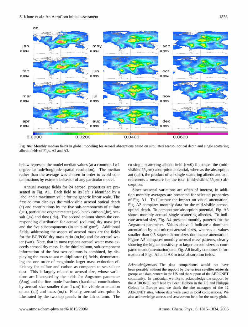
Fig. A6. Monthly median fields in global modeling for aerosol absorptions based on simulated aerosol optical depth and single scatteringalbedo fields of Figs. A2 and A3.

below represent the model median values (at a common 1×1degree latitude/longitude spatial resolution). The medianrather than the average was chosen in order to avoid con-taminations by extreme behavior of any particular model.

Annual average fields for 24 aerosol properties are pre-sented in Fig. A1. Each field to its left is identified by alabel and a maximum value for the generic linear scale. Thefirst column displays the mid-visible aerosol optical depth(a) and contributions by the five sub-components of sulfate(,su), particulate organic matter (,oc), black carbon (,bc), sea-salt (,ss) and dust (,du). The second column shows the cor-responding distribution for aerosol (column) dry mass (m)and the five subcomponents (in units of g/m2). Additionalfields, addressing the aspect of aerosol mass are the fieldsfor the BC/POM dry mass ratio (m,bo) and for aerosol wa-ter (wat). Note, that in most regions aerosol water mass ex-ceeds aerosol dry mass. In the third column, sub-componentinformation of the first two columns is combined, by dis-playing the mass-to-aot multiplicator (r) fields, demonstrat-ing the one order of magnitude larger mass extinction ef-ficiency for sulfate and carbon as compared to sea-salt ordust. This is largely related to aerosol size, whose varia-tions are illustrated by the fields for Angstrom parameter(Ang) and the fine mode-fractions (fractional contributionsby aerosol size smaller than 1µm) for visible attenuationor aot (a,f) and mass (m,f). Finally, aerosol absorption isillustrated by the two top panels in the 4th column. The

co-single-scattering albedo field (cw0) illustrates the (mid-visible/.55µm) absorption potential, whereas the absorptionaot (aab), the product of co-single scattering albedo and aot,represents a measure for the total (mid-visible/.55µm) ab-sorption.

Since seasonal variations are often of interest, in addi-tion monthly averages are presented for selected propertiesof Fig. A1. To illustrate the impact on visual attenuation,Fig. A2 compares monthly data for the mid-visible aerosoloptical depth. To demonstrate absorption potential, Fig. A3shows monthly aerosol single scattering albedos. To indi-cate aerosol size, Fig. A4 presents monthly patterns for theAngstrom parameter. Values above 1 indicate a dominantattenuation by sub-micron aerosol sizes, whereas at valuessmaller than 0.5 super-micron sizes dominante attenuation.Figure A5 compares monthly aerosol mass patterns, clearlyshowing the higher sensitivity to larger aerosol sizes as com-pared to aot (attenuation) and Fig. A6 finally combines infor-mation of Figs. A2 and A3 to total absorption fields.

Acknowledgements.The data comparisons would not havebeen possible without the support by the various satellite retrievalsgroups and data-centers in the US and the support of the AERONETcommunity. In particular, we like to acknowledge the support bythe AERONET staff lead by Brent Holben in the US and PhilippeGoloub in Europe and we thank the site managers of the 12AERONET sites, whose data were used in local comparisons. Wealso acknowledge access and assessment help for the many global



aerosol data-sets from satellite retrievals, including O. Torres forthe TOMS data, L. Remer for the MODIS data, R. Kahn andJ. Martonchik for the MISR data, J.-L. Deuze and P. Lallart forthe POLDER data, I. Geogdzhayev and M. Mishchenko for the2-channel AVHRR data and A. Ignatov for the 1-channel AVHRRdata. Also acknowledged is the support for this study by the EUPHOENICS project. The contributions of O. Boucher forms partof the Climate Prediction Programme of the UK Department forthe Environment, Food and Rural Affairs (DEFRA) under contractPECD 7/12/37.

Edited by: D. Grainger

References

Dentener, F., Kinne, S., Bonds, T., Boucher, O., Cofala, J., Gen-eroso, S., Ginoux, P., Gong, S., Hoelzemann, J., Ito, A., Marelli,L., Putaud, J.-P., Textor, C., and Schulz, M.: Emissions of pri-mary aerosol and precursor gases in the years 2000 and 1750:prescribed data-sets for AeroCom, Atmos. Chem. Phys. Discuss.,6, 2703–2763, 2006.

Deuze, J. L., Herman, M., and Goloub, P.: Characterization ofaerosols over ocean from POLDER/ADEOS-1, Geophys. Res.Lett., 26, 1421–1424, 1999.

Deuze, J. L., Breon, F. M., Devaux, C., Goloub, P., Herman, M.,Lafrance, B., Maignan, F., Marchand, A., Nadal, F., Perry, G.,and Tanre, D.: Remote sensing of aerosol over land surfaces fromPOLDER/ADEOS-1 polarized measurements, J. Geophys. Res.,106, 4912–4926, 2001.

Dubovik, O. and King, M.: A flexible inversion algorithm for theretrieval of aerosol optical properties from sun and sky radiancemeasurements, J. Geophys. Res., 105, 20 673–20 696, 2000.

Geogdzhyev, I., Mishchenko, M., Rossow, W., Cairns, B., andLacis, A.: Global 2-channel AVHRR retrieval of aerosol prop-erties over the ocean for the period of NOAA-9 observations andpreliminary retrievals using NOAA-7 and NOAA-11 data, J. At-mos. Sci., 59, 262–278, 2002.

Ignatov, A. and Nalli, N.: Aerosol retrievals from multi-satelliteAVHRR pathfinder (PATMOS) data-set for correcting remotelysensed sea surface temperature, J. Atmos. Ocean. Tech., 19,1986–2008, 2002.

Holben, B., Eck, T., Slutsker, I., Tanre, D., Buis, J., Vermote, E.,Reagan, J., Kaufman, Y., Nakajima, T., Lavenau, F., Jankowiak,I., and Smirnov, A.: AERONET, a federated instrument networkand data-archive for aerosol characterization, Rem. Sens. Envi-ron., 66, 1–66, 1998.

Houghton, J., Ding, Y., Griggs, D., Noguer, M., van der Linden,P., Dai, X., Maskell, K., Johnson, C., Meira Filho, L., Bruce,J., Lee, H., Callander, B., Haites, E., Harris, N., and Maskell,K.: Climate Change 2001, The Scientific Basis, an evaluation ofthe IPCC (International Panel on Climate Change), CambridgeUniversity Press, New York, 2001

Jeong, M. J. and Li, Z.: Quality, comparability and synergy anal-yses of global aerosol products, Part 1: AVHRR and TOMS, J.Geophys. Res., 110, 2005.

Kahn, R., Banerjee, P., McDonald, D., Diner, D. J.: Sensitivity ofmulti-angle imaging to aerosol optical depth and to pure particlesize distribution and composition over ocean, J.Geophys. Res.,103, 32 195–32 213, 1998.

Kaufman, Y., Tanre, D., Remer, L., Vermote, E., Chu, D., andHolben, B.: Operational remote sensing of tropospheric aerosolover the land from EOS-MODIS, J. Geophys. Res., 102, 17 051–17 061, 1997.

Kinne, S., Lohmann, U., Feichter, J., Timmreck, C., Schulz, M.,Ghan, S., Easter, R., Chin, M., Ginoux, P., Takemura, T., Tegen,I., Koch, D., Herzog, M., Penner, J., Pitari, G., Holben, B., Eck,T., Smirnov, A., Dubovik, O., Slutsker, I., Tanre, D., Torres, O.,Mishchenko, M., Geogdzhayev, I., Chu, D. A., and Kaufman,Y.: Monthly Averages of Aerosol Properties: A Global compari-son among models, satellite data and AERONET ground data, J.Geophys. Res, 108, 4634, 2003.

Martonchik, J. V., Diner, D. J., Kahn, R. A., Ackerman, T. P., Ver-straete, M. E., Pinty, B., and Gordon, H. R.: Techniques for theretreival of aerosol properties over land and ocean using multi-angle imaging, IEEE Trans. Geosci. Rem. Sensing, 36, 1212–1227, 1998.

Myhre, G., Stordal, F., Johnsrud, M., Diner, D. J., Geogdzhayev,I., Haywood, J. M., Holben, B., Holzer-Popp, T., Ignatov, A.,Kahn, R., Kaufman, Y., Loeb, N., Martonchik, J., Mishchenko,M., Nalli, N., Remer, L., Schroeter-Homscheid, M., Tanre, D.,Torres, O., and Wang, M.: Intercomparison of satellite retreivedaerosol optical depth over ocean during the period September1997 to December 2000, Atmos. Chem. Phys., 5, 1697–1719,2005.

Schulz, M., Textor, C., Kinne, S., Balkanski, Y., Bauer, S.,Berntsen, T., Berglen, T., Boucher, O., Dentener, F., Guibert,S., Isaksen, I. S. A., Iversen, T., Koch, D., Kirkevag, A., Liu,X., Montenaro, V., Myhre, G., Penner, J. E., Pitari, G., Reddy,S., Seland, O., Stier, P., and Takemura, T.: Radiative forcingby aerosols as derived from the AeroCom present-day and pre-industrial simulations, Atmos. Chem. Phys. Discuss., accepted,2006.

Tanre, D., Kaufman, Y. J., Herman, M., and Mattoo, S.: RemoteSensing of aerosol properties over ocean using the MODIS/EOSspectral radiances, J. Geophys. Res., 102, 16 971–16 988, 1997.

Textor, C. , Schulz, M., Guibert, S., Kinne, S., Balkanski, Y., Bauer,S., Berntsen, T., Berglen, T., Boucher, O., Chin, M., Dentener,F., Diehl, T., Easter, R., Feichter, H., Fillmore, D., Ghan, S., Gi-noux, P., Gong, S., Grini, A., Hendricks, J., Horowitz, L., Huang,P., Isaksen, I., Iversen, T., Kloster, S., Koch, D., Kirkevg, A.,Kristjansson, J. E., Krol, M., Lauer, A., Lamarque, J. F., Liu,X., Montanaro, V., Myhre, G., Penner, J., Pitari, G., Reddy, S.,Seland, Ø., Stier, P., Takemura, T., and Tie, X.: Analysis andquantification of the diversities of aerosol life cycles within Ae-roCom, Atmos. Chem. Phys., 6, 1777–1813, 2006.

Torres, O., Barthia, P. K., Herman, J. R., Sinyuk, A., Ginoux, P.,and Holben, B.: A long-term record of aerosol optical depthfrom TOMS observationsand comparisons to AERONET mea-surements, J. Atmos. Sci., 59, 398–413, 2002.


an aerocom initial assessment – optical properties in

Documents