an all-fiber image-reject homodyne coherent doppler wind...

General rights Copyright and moral rights for the publications made accessible in the public portal are retained by the authors and/or other copyright owners and it is a condition of accessing publications that users recognise and abide by the legal requirements associated with these rights.

• Users may download and print one copy of any publication from the public portal for the purpose of private study or research. • You may not further distribute the material or use it for any profit-making activity or commercial gain • You may freely distribute the URL identifying the publication in the public portal

If you believe that this document breaches copyright please contact us providing details, and we will remove access to the work immediately and investigate your claim.

Downloaded from orbit.dtu.dk on: Aug 20, 2018

An all-fiber image-reject homodyne coherent Doppler wind lidar

Foroughi Abari, Farzad; Pedersen, Anders Tegtmeier; Mann, Jakob

Published in:Optics Express

Link to article, DOI:10.1364/OE.22.025880

Publication date:2014

Document VersionPublisher's PDF, also known as Version of record

Link back to DTU Orbit

Citation (APA):Foroughi Abari, F., Pedersen, A. T., & Mann, J. (2014). An all-fiber image-reject homodyne coherent Dopplerwind lidar. Optics Express, 22(21), 25880-25894. DOI: 10.1364/OE.22.025880

http://dx.doi.org/10.1364/OE.22.025880

http://orbit.dtu.dk/en/publications/an-allfiber-imagereject-homodyne-coherent-doppler-wind-lidar(3efb8d80-f1b1-4f16-9ab2-34eafaffc7d9).html

An all-fiber image-reject homodynecoherent Doppler wind lidar

Cyrus F. Abari, ∗ Anders T. Pedersen, and Jakob MannDepartment of Wind Energy, Technical University of Denmark, Roskilde DK-4000, Denmark

∗[email protected]

Abstract: In this paper, we present an alternative approach to the down-conversion (translation) of the received optical signals collected by theantenna of an all-fiber coherent Doppler lidar (CDL). The proposed method,widely known as image-reject, quadrature detection, or in-phase/quadrature-phase detection, utilizes the advances in fiber optic communications suchthat the received signal can be optically down-converted into basebandwhere not only the radial velocity but also the direction of the movementcan be inferred. In addition, we show that by performing a cross-spectralanalysis, enabled by the presence of two independent signal observationswith uncorrelated noise, various noise sources can be suppressed and amore simplified velocity estimation algorithm can be employed in thespectral domain. Other benefits of this architecture include, but are notlimited to, a more reliable measurement of radial velocities close to zeroand an improved bandwidth. The claims are verified through laboratoryimplementation of a continuous wave CDL, where measurements both on ahard and diffuse target have been performed and analyzed.

© 2014 Optical Society of America

OCIS codes:(280.3640) Lidar; (010.3640) Lidar; (120.4640) Optical instruments.

References and links1. G. Fiocco and L. D. Smullin, “Detection of scattering layers in the upper atmosphere (60-140 km) by optical

radar,” Nature (London)199(1), 1275–1276 (1963).2. A. V. Jelalian,Laser radar systems (Boston Artech, 1992).3. ZephIR 300 technical specifications, (ZephIR Lidar, 2014).http://www.zephirlidar.com/resources/technical-specs.4. WINDCUBE V2, a 200m vertical wind Doppler lidar, (Leosphere, 2014).

http://www.leosphere.com/products/vertical-profiling/windcube-v2.5. WINDAR functional specifications, (WINDAR PHOTONICS, 2014).http://www.windarphotonics.com/product.6. F. Bingol, J. Mann, and D. Foussekis, “Conically scanning lidar error in complex terrain,” Meteorologische

Zeitschrift18(2), 189–195 (2009).7. S. Lang and E. McKeogh, “Lidar and sodar measurements of wind speed and direction in upland terrain for wind

energy purposes,” Remote Sens.3(9), 1871–1901 (2011).8. T. Mikkelsen, N. Angelou, K. Hansen, M. Sjoholm, M. Harris, C. Slinger, P. Hadley, R. Scullion, G. Ellis, and

G. Vives, “A spinner-integrated wind lidar for enhanced wind turbine control,” Wind Energy16(4), 625–643(2013).

9. D. Schlipf, D. J. Schlipf, and M. Kuhn, “Nonlinear model predictive control of wind turbines using lidar,” WindEng.16(7), 1107–1129 (2012).

10. I. Antoniou, S. M. Pedersen, and P. B. Enevoldsen, “Wind shear and uncertainties in power curve measurementand wind resources,” Wind Eng.33(5), 449–468 (2010).

11. C. J. Karlsson, F. A. Olsson, D. Letalick, and M. Harris, “All-fiber multifunction continuous-wave coherent laserradar at 1.55µm for range, speed, vibration, and wind measurements,” Appl. Opt.39(21), 3716–3726 (2000).

12. G. N. Pearson, P. J. Roberts, J. R. Eacock, and M. Harris, “Analysis of the performance of a coherent pulsed fiberlidar for aerosol backscatter applications,” Appl. Opt.41(30), 6442–6450 (2002).

#217118 - $15.00 USD Received 17 Jul 2014; revised 6 Oct 2014; accepted 8 Oct 2014; published 14 Oct 2014(C) 2014 OSA 20 October 2014 | Vol. 22, No. 21 | DOI:10.1364/OE.22.025880 | OPTICS EXPRESS 25880

13. P. Lindelow, “Fiber based coherent lidars for remote wind sensing,” PhD dissertation, Dept. of Photon. Eng.,Tech. Univ. of Denmark, Lyngby, Denmark, 2007.

14. S. F. Jacobs, “Optical heterodyne (coherent) detection,” Am. J. Phys.56(3), 235–245 (1988).15. O. E. DeLange, “Optical heterodyne detection,” IEEE Spectrosc.5(10), 77–85 (1968).16. B. Razavi, “Design considerations for direct-conversion receivers,” IEEE Trans. Circuits Syst. II: Analog Digit.

Signal Process.44(6), 428–435 (1997).17. L. Richter, H. Mandelberg, M. Kruger, and P. McGrath, “Linewidth determination from self-heterodyne measure-

ments with subcoherence delay times,” IEEE J. Quantum Electron.22(11), 2070–2074 (1986).18. M. Harris, G. N. Pearson, K. D. Ridley, C. J. Karlsson, F. A. Olsson, and D. Letalick “Single-particle laser

Doppler anemometry at 1.5µm,” Appl. Opt.40(6), 969–973 (2001).19. J. R. Barry and E. A. Lee, “Performance of coherent optical receivers,” Proc. IEEE78(8), 1369–1394 (1990).20. A. Valle and L. Pesquera, “Relative intensity noise of multitransverse-mode vertical-cavity surface-emitting

lasers,” IEEE Photon. Technol. Lett.13(4), 272–274 (2001).21. R. Stierlin, R. Battig, P. D. Henchoz, and H. P. Weber, “Excess-noise suppression in a fiber-optic balanced het-

erodyne detection system,” Opt. Quantum Electron.18(6), 445–454 (1986).22. L. Ma, Y. Hu, S. Xiong, Z. Meng, and Z. Hu, “Intensity noise and relaxation oscillation of a fiberlaser sensor

array integrated in a single fiber,” Opt. Lett.35(1), 1795–1797 (2010).23. G. A. Cranch, M. A. Englund, and C. K. Kirkendal, “Intensity noise characteristics of erbium-doped distributed-

feedback lasers,” IEEE J. Quantum Electron.39(12), 1579–1587 (2003).24. A. D. McCoy, L. B. Fu, M. Ibsen, B. C. Thomsen, and D. J. Richardson, “Relaxation oscillation noise suppression

in fiber DFB lasers using a semiconductor optical amplifier,” in Conference on Lasers and Electro-Optics, 2004OSA CLEO Poster Session II (Optical Society of America, 2004), page CWA56.

25. P. J. Rodrigo and C. Pedersen. ”Comparative study of the performance of semiconductor laser based coherentDoppler lidars,” Proc. SPIE8241, 824112 (2012).

26. B. J. Rye and R. M. Hardesty, “Discrete spectral peak estimation in incoherent backscatter heterodyne lidar.I: Spectral accumulation and the Cramer-Rao lower bound,” IEEE Trans. Geosci. Remote Sens.31(1), 16–27(1993).

27. J. M. B. Dias and J. M. N. Leitao, “Nonparametric estimation of mean Doppler and spectral width,” IEEE Trans.Geosci. Remote Sens.38(1), 271–282 (2000).

28. M. H. Hayes,Statistical Digital Signal Processing and Modeling (John Wiley & Sons, 1996).29. A. T. Pedersen, C. F. Abari, J. Mann, and T. Mikkelsen, “Theoretical and experimental signal-to-noise ratio

assessment in new direction sensing continuous-wave Doppler lidar,” in J. Phys.: Conf. Ser., Vol. 524 (IOPPublishing, 2014), paper 012004.

30. M. Harris, G. N. Pearson, J. M. Vaughan, and D. Letalick, “The role of laser coherence length in continuous-wavecoherent laser radar,” J. Mod. Opt.45(8), 1567–1581 (2009).

31. B. Moslehi, “Analysis of optical phase noise in fiber-optic systems employing a laser source with arbitrary co-herence time,” J. Lightw. Technol.4(9), 1334–1351 (1986).

32. C. A. Hill, M. Harris, and K. D. Ridley, “Fiber-based 1.5µm lidar vibrometer in pulsed and continuous modes,”Appl. Opt.46(20), 4376–4385 (2007).

33. C. Allen, Y. Cobanoglu, S. K. Chong, and S. Gogineni, “Development of a 1310-nm, coherent laser radar withRF pulse compression,” in Proceedings of IEEE Geoscience and Remote Sensing Symposium (IEEE, 2000), pp.1784–1786.

34. L. G. Kazovsky, L. Curtis, W. C. Young, and N. K. Cheung, “All-fiber 90 optical hybrid for coherent communi-cations,” Appl. Opt.26(3), 437–439 (1987).

35. D. O. Hogenboom and C. A. DiMarzio, “Quadrature detection of a Doppler signal,” Appl. Opt.37(13), 2569–2572 (1998).

36. N. Angelou, C. F. Abari, J. Mann, T. Mikkelsen, and M. Sjoholm, “Challenges in noise removal from Dopplerspectra acquired by a continuous-wave lidar,” Presented at the 26th International Laser Radar Conference, PortoHeli, Greece, 25-29 June 2012.

1. Introduction

Light detection and ranging (lidar) instruments have been in use for remote sensing of atmo-spheric conditions, including the atmospheric boundary layer (ABL), for about five decades.For instance, Fiocco and Smullin [1] demonstrated one of the early application of lidars (alsoknown as optical radar) in atmospheric characterizations and meteorological observations.Wind lidars were already employed in early 1970s [2]. Following advances in fiber optic com-munications, where lasers with wavelengths close to 1550 nm are used, this technology has beenextensively used in all-fiber CDLs. Commercial examples of such systems are widely available:for instance, ZephIR from ZephIR Lidar [3], Windcube from Leosphere [4], and WindEye from


WINDAR Photonics [5] are examples of all-fiber CDLs. The all-fiber 1550 nm CDLs have amaster oscillator power amplifier architecture (MOPA) where a compact laser source, known asthe master oscillator (MO), is utilized for the generation of a highly coherent light. Examplesof MOs are distributed feedback (DFB) fiber or semiconductor lasers. DFB lasers have a smallform factor and provide high sensitivity, robustness, and low levels of phase noise. The fiberoptic technology, used in optical communications industry, is employed for the generation, am-plification, transmission, and manipulation of the laser beam in all-fiber CDLs. Applications ofCDLs in the wind industry cover, but are not limited to, the measurement of wind velocitiesin terrain for the characterization and optimization of wind turbine installation (wind resourceassessment) [6, 7], the measurement of the incoming wind flow for optimal wind turbine yawand pitch control [8, 9], and power curve verification [10].

Typically, there are two major variants of mono-static CDLs used for wind measurements,i.e., continuous wave (CW) and pulsed. In CW CDLs ranging is achieved by translating the endfacet of the delivery fiber along the optical axis of the telescope [11]. Thus, ranging is achievedby focusing the laser beam on the range of interest. On the other hand, pulsed lidars emit a laserpulse for wind flow characterizations [12]. In such systems, ranging is achieved by range gatingthe received signals, i.e., the collected scattering from aerosol particles [13]. In both types ofsystems, the backscatter from aerosol particles are collected through a telescope which passesthem on to the following stages for further processing.

Due to numerous advantages provided by digital signal processing algorithms, the detectedsignals are typically digitized for further treatment. However, the available analog-to-digitalconverters (A/D) have limited bandwidth (BW) that is far below the laser frequency, conven-tionally known as the carrier frequency. Besides, the opto-electronic components, such as pho-todetectors have limited BW and cannot follow signal fluctuations in the THz region. As aresult, it is imperative to down-convert the optical signals into lower radio frequency (RF)spectrum known as intermediate frequency (IF) or baseband, also known as zero-IF. Coherentreceivers achieve this by mixing (beating) the reflections with a local oscillator (LO) signal,usually derived from the MO. Depending on the LO frequency and the front-end treatmentof the signals, various architectures may be realized. In fact, the optical coherent detection is”simply an extension into the optical region, of a well-known radio-frequency technique usedin superheterodyne receiver”. [14]

Depending on the frequency where the optical signal is translated [15] the architectures inCDLs may be categorized into two main classes: direct-conversion (homodyne) and hetero-dyne architectures. In homodyne receivers, the LO and signal carrier frequencies are equal. Inheterodyne receivers, the carrier frequency is different from the LO’s. A homodyne or hetero-dyne receiver may be realized through either real mixing or in-phase/quadrature-phase (I/Q)mixing, also known as complex mixing. The complex mixing process is also known as theimage-reject or quadrature mixing principle. The inability to perform an image rejection (andthus real mixing) in telecommunications results in possible corruption of the transmitted infor-mation because the two sides of the band overlap and interfere [16]. In CDLs it results in asymmetric spectrum where the sign of the radial wind velocity cannot be discriminated whichis a rather serious issue for certain applications. To solve the sign ambiguity, a few receiverarchitectures can be employed, the most popular of which are heterodyne receivers with IFsampling and homodyne receivers with complex mixing. Heterodyne mixing with IF samplingis a well-known and widely used approach for signal detection in CDLs.

In this paper, we show that by employing a direct image-reject architecture in a CW CDL,made feasible through commercially available components for optical communications, a morerobust and accurate CDL can be prototyped. The result is a system that has twice the BW as ex-isting CDLs that employ heterodyning with IF sampling for a similar system configuration. In


addition, the prototype system provides a better estimate of radial velocities close to zero wherethe signal is contaminated by noise in heterodyne receivers. Furthermore, it is shown that byperforming a cross-spectral analysis between the in-phase and quadrature-phase components,the noise sources (mainly the shot noise) can be suppressed and a less signal processing inten-sive algorithm employed to extract the radial velocity information. Although the focus of thepaper is on CW CDLs many of the principles can be applied to a pulsed CDL with no or minormodifications.

The paper is divided into several sections. In Section 2, we adopt a simple but efficient signalmodel associated with coherent detection in an all-fiber homodyne CW CDL with real mixingto present the concepts and lay a mathematical framework. In Section 3, we present the image-reject homodyne receiver and analyze its theoretical performance with respect to receivers withreal mixing such as the one described in Section 2. A laboratory prototype of an all-fiber image-reject homodyne CW CDL, as described in this paper, is presented in Section 4 where a fewmeasurement results on hard and diffused target are presented as a proof of concept. Throughoutthe paper, an effort has been made to emphasize the most important parameters affecting theCDL performance for the discussed architectures. Meanwhile, wherever deemed appropriate,we have ignored the topics secondary to the results presented in this paper. We have also adopteda number of simplifications without sacrificing the generality and applicability of the results.The optical and electronic components in this paper are assumed to be lossless and ideal unlessotherwise specified in the text.

2. Coherent detection and signal modeling

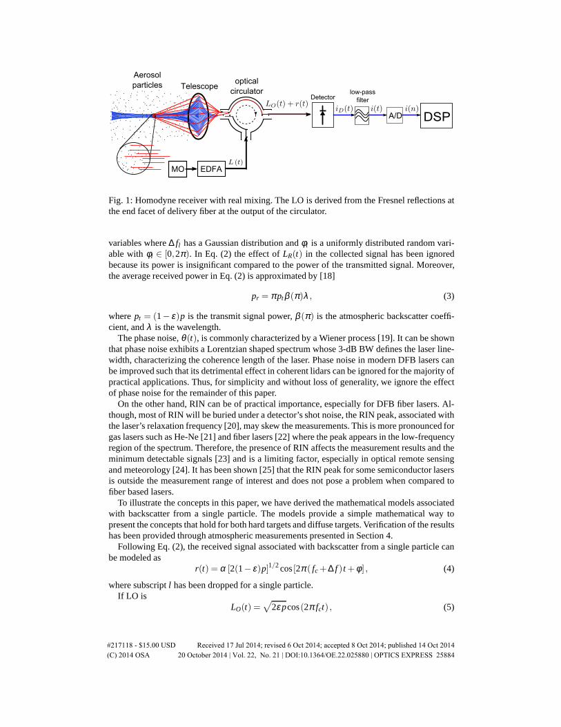
Before analyzing the image-reject receiver architectures, it is worthwhile to adopt appropriatetransmit and receive signal models associated with a CW CDL in a MOPA configuration. Fig.1 illustrates one of the simplest receiver architectures adopted for such systems. In this system,the laser source signal, MO, is modeled after the fundamental mode of an optical resonator,i.e., TEM00 [15], where the transverse irradiance has a Gaussian distribution and the longitu-dinal intensity is Lorentzian. Irrespective of the temporal irradiance shape associated with thetransmitted laser signal, we can adopt the following mathematical model in time domain for theelectric field fluctuations of the optical signal at the output of the erbium doped fiber amplifier(EDFA):

L(t) =√

2pcos[2π fct +θ (t)]+LR(t), (1)

wherep is the optical signal power,fc is the laser frequency (also known as the carrier fre-quency),θ (t) is the laser phase noise that defines the laser line width [17], andLR(t) is therelative intensity noise (RIN) of the laser. After passing through the optical circulator,L(t) issplit into a transmit signals(t) and LO signalLO(t). LO in this particular system configurationis derived by collecting the back reflections from the end facet of the delivery fiber, i.e., the fiberat the input of the telescope. The LO power can be adjusted by polishing the end facet of thedelivery fiber [11] at the desired angle. Thus, the transmitted signal,s(t), through the telescopeis a major fraction ofL(t) wheres(t) =

√1− εL(t). Furthermore, 0< ε < 1 is the splitting

ratio that controls the LO power. For reflections from a diffuse target such as backscatter fromaerosol particles in the air the received signal for the collected light by the telescope can bemodeled as

r(t) = [2(1− ε)p]1/2L−1

∑l=0

αl cos[2π ( fc +∆ fl) t +θ (t)+φl] , (2)

whereαl is the net optical attenuation ,∆ fl is the Doppler shift due to motion,φl is the phasefactor associated with thelth aerosol particle, andL is the number of aerosol particles in themeasurement volume. Furthermore,αl , ∆ fl , andφl can be modeled as independent random


A/D

Detector

DSP

optical

circulator low-pass

filter

MO EDFA

Aerosol

particles Telescope

Fig. 1: Homodyne receiver with real mixing. The LO is derived from the Fresnel reflections atthe end facet of delivery fiber at the output of the circulator.

variables where∆ fl has a Gaussian distribution andφl is a uniformly distributed random vari-able withφl ∈ [0,2π). In Eq. (2) the effect ofLR(t) in the collected signal has been ignoredbecause its power is insignificant compared to the power of the transmitted signal. Moreover,the average received power in Eq. (2) is approximated by [18]

pr = π ptβ (π)λ , (3)

wherept = (1− ε)p is the transmit signal power,β (π) is the atmospheric backscatter coeffi-cient, andλ is the wavelength.

The phase noise,θ (t), is commonly characterized by a Wiener process [19]. It can be shownthat phase noise exhibits a Lorentzian shaped spectrum whose 3-dB BW defines the laser line-width, characterizing the coherence length of the laser. Phase noise in modern DFB lasers canbe improved such that its detrimental effect in coherent lidars can be ignored for the majority ofpractical applications. Thus, for simplicity and without loss of generality, we ignore the effectof phase noise for the remainder of this paper.

On the other hand, RIN can be of practical importance, especially for DFB fiber lasers. Al-though, most of RIN will be buried under a detector’s shot noise, the RIN peak, associated withthe laser’s relaxation frequency [20], may skew the measurements. This is more pronounced forgas lasers such as He-Ne [21] and fiber lasers [22] where the peak appears in the low-frequencyregion of the spectrum. Therefore, the presence of RIN affects the measurement results and theminimum detectable signals [23] and is a limiting factor, especially in optical remote sensingand meteorology [24]. It has been shown [25] that the RIN peak for some semiconductor lasersis outside the measurement range of interest and does not pose a problem when compared tofiber based lasers.

To illustrate the concepts in this paper, we have derived the mathematical models associatedwith backscatter from a single particle. The models provide a simple mathematical way topresent the concepts that hold for both hard targets and diffuse targets. Verification of the resultshas been provided through atmospheric measurements presented in Section 4.

Following Eq. (2), the received signal associated with backscatter from a single particle canbe modeled as

r(t) = α [2(1− ε)p]1/2cos[2π ( fc +∆ f )t +φ ] , (4)

where subscriptl has been dropped for a single particle.If LO is

LO(t) =√

2ε pcos(2π fct) , (5)


1/f+DC offset

RIN Shot noise

level

(a) CTFT

1/f+DC offset

RIN Shot noise

level

(b) DFT

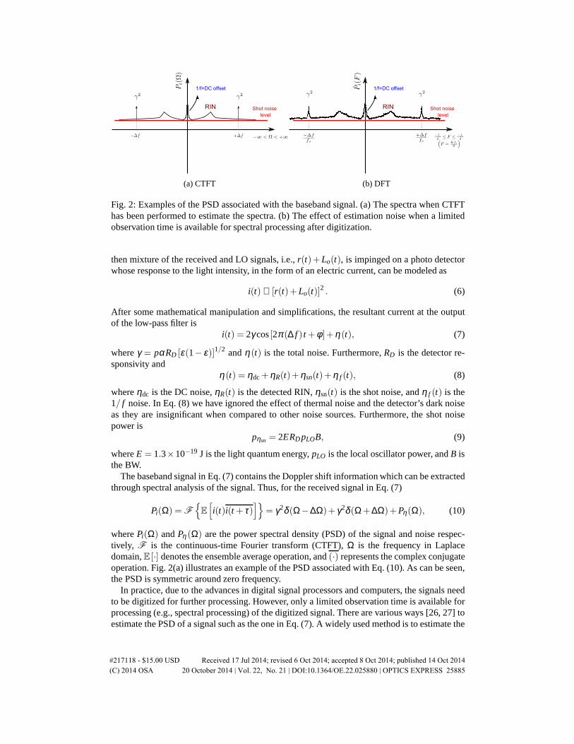
Fig. 2: Examples of the PSD associated with the baseband signal. (a) The spectra when CTFThas been performed to estimate the spectra. (b) The effect of estimation noise when a limitedobservation time is available for spectral processing after digitization.

then mixture of the received and LO signals, i.e.,r(t)+Lo(t), is impinged on a photo detectorwhose response to the light intensity, in the form of an electric current, can be modeled as

i(t) ∝ [r(t)+Lo(t)]2 . (6)

After some mathematical manipulation and simplifications, the resultant current at the outputof the low-pass filter is

i(t) = 2γ cos[2π (∆ f ) t +φ ]+η(t), (7)

whereγ = pαRD [ε(1− ε)]1/2 andη(t) is the total noise. Furthermore,RD is the detector re-sponsivity and

η(t) = ηdc+ηR(t)+ηsn(t)+η f (t), (8)

whereηdc is the DC noise,ηR(t) is the detected RIN,ηsn(t) is the shot noise, andη f (t) is the1/ f noise. In Eq. (8) we have ignored the effect of thermal noise and the detector’s dark noiseas they are insignificant when compared to other noise sources. Furthermore, the shot noisepower is

pηsn = 2ERD pLOB, (9)

whereE = 1.3×10−19 J is the light quantum energy,pLO is the local oscillator power, andB isthe BW.

The baseband signal in Eq. (7) contains the Doppler shift information which can be extractedthrough spectral analysis of the signal. Thus, for the received signal in Eq. (7)

Pi(Ω) = F

E

[

i(t)i(t + τ)]

= γ2δ (Ω−∆Ω)+ γ2δ (Ω+∆Ω)+Pη(Ω), (10)

wherePi(Ω) andPη(Ω) are the power spectral density (PSD) of the signal and noise respec-tively, F is the continuous-time Fourier transform (CTFT),Ω is the frequency in Laplacedomain,E [·] denotes the ensemble average operation, and(·) represents the complex conjugateoperation. Fig. 2(a) illustrates an example of the PSD associated with Eq. (10). As can be seen,the PSD is symmetric around zero frequency.

In practice, due to the advances in digital signal processors and computers, the signals needto be digitized for further processing. However, only a limited observation time is available forprocessing (e.g., spectral processing) of the digitized signal. There are various ways [26, 27] toestimate the PSD of a signal such as the one in Eq. (7). A widely used method is to estimate the


spectra through periodograms [28], which when applied to the digitized version of the signal inEq. (7), results in

Pi(K) =fs

M

M−1

∑m=0

|I(K)|2 , (11)

whereK is the discrete frequency component,M is the number of averages, andfs is the sam-pling frequency. In addition,I(K) is the discrete Fourier transform (DFT) defined as

I(K) =1N

N−1

∑n=0

i(n)exp(

−2π jnN

K)

, (12)

whereN is the number of DFT points. Compared to Eq. (10),

Pi(K) = Pi (ΩK)+ηest(K), (13)

whereηest(K) is the estimation noise andΩK = K fsN . For the shot-noise limited operational

mode, where the effect of all other noise sources are neglected,ηest(K) can be modeled as aGaussian random variable [29] where

µηest (K) = Eηest(K)= ηsn (ΩK) ,

σηest (K) =Pi (ΩK)√

M.

(14)

Fig. 2(b) shows an example of an estimated PSD for the signal in Eq. (7).The ability to detect the Doppler shift in practice depends on the performance of the esti-

mation algorithm that can discriminate the signal information from the noise, especially, theestimation noise. As a result, it seems necessary to define a new quantity:

SENRi =Pi(KD)−Pη(KD)

σηest (K)|(K 6=KD), (15)

where SENRi is the signal-to-estimation-noise-ratio andKD =±⌊∆ ffs⌋N, the frequency associ-

ated with the Doppler peak. Please note that SENR is different from (the commonly used)

SNRi =

∫ +∞−∞ Pi (Ω) dΩ− pη

pη, (16)

wherepη =∫ +∞−∞ Pη (Ω) dΩ. For a shot-noise limited operation, where the effect of other noise

sources and unwanted signals is ignored, and assuming a flat spectra the SNR for the presentedhomodyne receiver with real mixing is

SNRi =α2RD(1− ε)p

EB. (17)

One of the major sources of unwanted signals is the non-ideal behavior of optical componentssuch as the optical circulator. For instance, due to the presence of phase noise and cross-talk inoptical circulators the estimated signal may suffer from interferometric noise [30, 31]. Reflec-tions from optical components such as telescope lenses can also be compounding. A thoroughanalysis of SENR has been performed in [29] from which it can be inferred that the SENR forthe simple homodyne system, described in this section, is

SENRi =

√Mα2RD(1− ε)p

E= B

√MSNRi. (18)


A/D

DSP

90 o

Balanced

mixer

A/DBalanced

mixer

Circulator

MO EDFA

I/Q mixerAerosol

particles Telescope

Fig. 3: The schematic of the image-reject homodyne receiver.

As shown in Eq. (16), SNR refers to the ratio of the signal power and the instrument noisepower (e.g., shot-noise). In spectral analysis, however, SENR seems to be the major player indetermining how well the signal can be estimated when buried in estimation noise.

Despite its many advantages, the above-modeled system suffers from an inability to dis-criminate the direction of travel, i.e., the sign of the radial velocity. This is evident from theexample PSDs illustrated in Figs. 2(a)-2(b), in which the presence of the image componentof the Doppler signal masks the sign of the radial velocity. To extract the direction of travel,other receiver architectures need to be implemented. Examples of such systems are heterodynereceivers with IF sampling [32], super heterodyne receivers [33], and image-reject homodynereceivers. In the following sections we have presented a detailed analysis of an all-fiber image-reject homodyne receiver. The presented system not only resolves the sign ambiguity, but it alsobenefits from a novel approach in signal processing that eliminates the major noise sources andsimplifies extraction of the Doppler information from the signal. Additionally, through proto-typing the system we will demonstrate its performance for a number of different measurementscenarios, including measurement on hard and diffuse targets.

3. Image-reject architecture

To resolve the ambiguity associated with the direction of travel, an image-reject homodynereceiver can be utilized. In image-reject homodyne receivers, the return signal is mixed withtwo realizations of the LO signal where one realization is exactly 90 degrees out of phase withrespect to the other one. This concept is widely used in radio systems [16] and in optical com-munications [34]. The idea has also been tested as a solution in CDLs using open space optics.For instance, it has been shown [35] that by using a circularly polarized light one can attain thein-phase and quadrature-phase LO realizations required for this principle. The reported resultswere based on measurements on a hard target in a laboratory environment. However, to the bestof our knowledge, this is the first time an all-fiber system implementation of a CDL employingan image-reject homodyne architecture has been reported in literature where measurements forboth hard and diffuse targets have been successfully performed.

Fig. 3 provides an illustration of the system implementation for an all-fiber image-rejectarchitecture. In contrast to the homodyne receiver illustrated in Fig. 1, the LO signal in thissystem is not derived from Fresnel reflection at the end facet of the delivery fiber at the output ofthe optical circulator. Instead, two realizations of the LO with equal power are obtained throughan I/Q mixer. The I/Q mixer has two fundamental roles. First, it provides two realization of theLO required for in-phase and quadrature-phase components. Second, it utilizes two balanced


Coupler

+-

Balanced

detector

low-pass

filter

Balanced

mixer

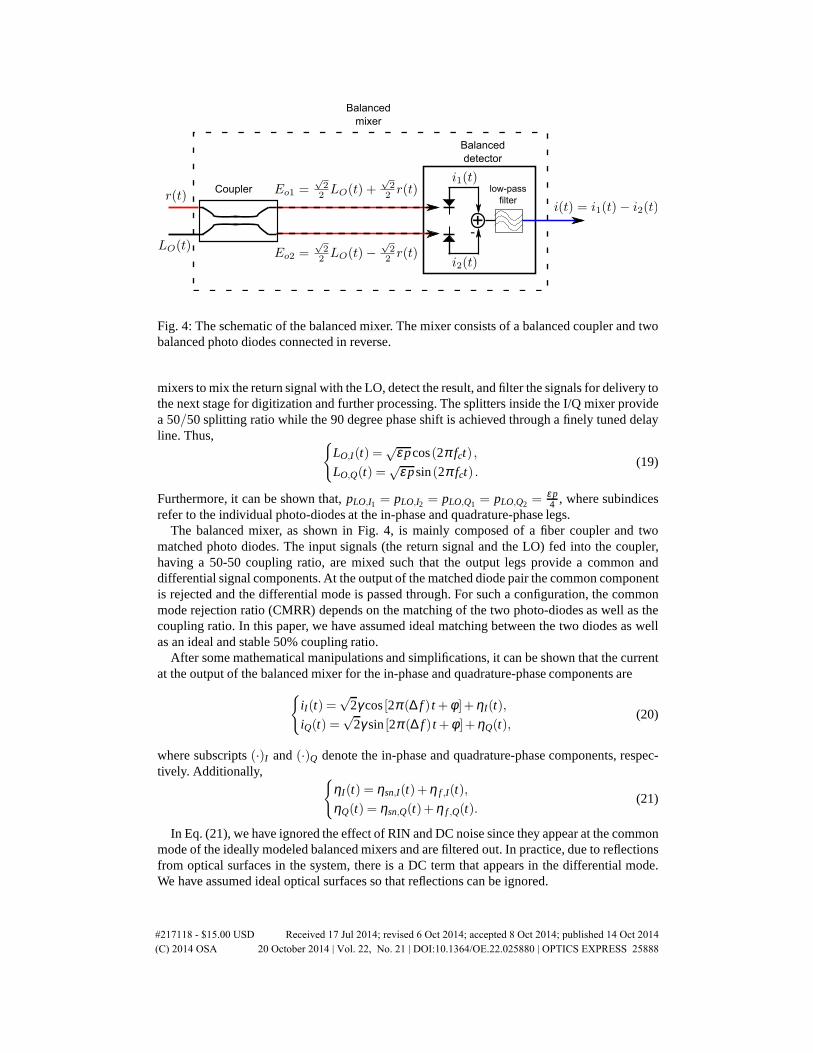
Fig. 4: The schematic of the balanced mixer. The mixer consists of a balanced coupler and twobalanced photo diodes connected in reverse.

mixers to mix the return signal with the LO, detect the result, and filter the signals for delivery tothe next stage for digitization and further processing. The splitters inside the I/Q mixer providea 50/50 splitting ratio while the 90 degree phase shift is achieved through a finely tuned delayline. Thus,

LO,I(t) =√ε pcos(2π fct) ,

LO,Q(t) =√

ε psin(2π fct) .(19)

Furthermore, it can be shown that,pLO,I1 = pLO,I2 = pLO,Q1 = pLO,Q2 =ε p4 , where subindices

refer to the individual photo-diodes at the in-phase and quadrature-phase legs.The balanced mixer, as shown in Fig. 4, is mainly composed of a fiber coupler and two

matched photo diodes. The input signals (the return signal and the LO) fed into the coupler,having a 50-50 coupling ratio, are mixed such that the output legs provide a common anddifferential signal components. At the output of the matched diode pair the common componentis rejected and the differential mode is passed through. For such a configuration, the commonmode rejection ratio (CMRR) depends on the matching of the two photo-diodes as well as thecoupling ratio. In this paper, we have assumed ideal matching between the two diodes as wellas an ideal and stable 50% coupling ratio.

After some mathematical manipulations and simplifications, it can be shown that the currentat the output of the balanced mixer for the in-phase and quadrature-phase components are

iI(t) =√

2γ cos[2π (∆ f ) t +φ ]+ηI(t),

iQ(t) =√

2γ sin[2π (∆ f ) t +φ ]+ηQ(t),(20)

where subscripts(·)I and(·)Q denote the in-phase and quadrature-phase components, respec-tively. Additionally,

ηI(t) = ηsn,I(t)+η f ,I(t),

ηQ(t) = ηsn,Q(t)+η f ,Q(t).(21)

In Eq. (21), we have ignored the effect of RIN and DC noise since they appear at the commonmode of the ideally modeled balanced mixers and are filtered out. In practice, due to reflectionsfrom optical surfaces in the system, there is a DC term that appears in the differential mode.We have assumed ideal optical surfaces so that reflections can be ignored.


1/f noise

Shot noise

level

(a) Autospectrum, positive Doppler shift

1/f noise

Shot noise

level

(b) Autospectrum, negative Doppler shift

Fig. 5: Examples of the estimated PSD associated with the baseband signal. (a) The spectrawhen the radial direction of travel associated with the target is positive. (b) Because the radialdirection of travel is away from the telescope, a negative Doppler shift is measured.

The signal pair in Eq. (20) can be combined to make a complex valued signal such that,

iIQ(t) =√

2γ cos(2π∆ f t +φ)+ηI(t)+ j[√

2γ sin(2π∆ f t +φ)+ηQ(t)]

, (22)

where j =√−1. Moreover, it can be shown that

PiIQ(Ω) = 2γ2δ (Ω−∆Ω)+PηI(Ω)+PηQ(Ω),

PiIQ(K) = PiIQ(ΩK)+ηest(K),(23)

and [29]

SENRiIQ =√

MSNRiIQ =

√Mα2RD(1− ε)p

E. (24)

Fig. 5(a)-5(b) show examples of the PSD associated with Eq. (23). As can be seen, the PSDsare not symmetric. Also, when compared to the PSDs in Fig. 2(a)-2(b), they are free from RINand DC noise, thanks to the balanced mixer.

Although the shot noise exhibits a flat spectrum, it is usually shaped due to the presence offilters and electronic components. As a result, to extract the Doppler information it is necessaryto whiten the noise [36]. Among other things, noise whitening is a signal processing intensivealgorithm and adds to the uncertainty of radial velocity estimation. The image-reject architec-ture makes the noise whitening redundant due to the availability of two signal observations withindependent noise sources. As a result, by performing a cross-spectral analysis between the in-phase and quadrature-phase components we have shown that the signal information, includingthe direction of travel, is contained in the imaginary part of the result. Thus,

ℑ[

PiI iQ(Ω)]

=12

γ2 [δ (Ω+∆Ω)− δ (Ω−∆Ω)], (25)

wherePiI iQ(Ω) = F

(

E

[

II(Ω)IQ(Ω)])

, (26)

andℑ [·] represents the imaginary component. Furthermore,

PiI iQ(K) =fs

M

M−1

∑m=0

II(K)IQ(K) = PiI iQ(ΩK)+ηest,IQ(K), (27)


(a) Cross-spectrum, positive Doppler shift (b) Cross-spectrum, negative Doppler shift

Fig. 6: Examples of the estimated cross-spectra of the in-phase and quadrature-phase signalcomponents in baseband. (a) Positive Doppler shift. (b) Negative Doppler shift.

where, similar to Eq. (14),ηest,IQ is a zero-mean Gaussian random variable withσ2ηest,IQ

. More-over, following [29] it can be shown that

SENRiI iQ =

√2Mα2RD(1− ε)p

2E. (28)

One of the main advantages of the cross-spectral analysis is elimination of uncorrelated noisesources including the shot-noise. Elimination of background noise simplifies the estimationalgorithms (including background noise whitening) to extract the Doppler information. It alsoreduces the number of frequency bins by a factor of 2, which essentially translates into a moreefficient storage of spectral data. Moreover, due to the elimination of 1/f noise and DC noisearound zero-frequency component, a better estimate of the radial velocities close to zero can beperformed. The experimental results, carried out for the measurement of the vertical componentof the wind, support the above mentioned claim and will be published in a future paper. Thisis in contrast to other available system implementations, such as the heterodyne receiver withIF sampling employing an AOM, where the system suffers from added noise by the additionalactive component (that is, the AOM) and non-ideal filters such as notch filters. Despite its manyadvantages, the cross-spectral approach suffers from an inherent SENR loss, viz.,

√2

2 , [29] thatbecomes evident when comparing Eq. (24) and Eq. (28).

4. Experimental results

An all-fiber prototype of the proposed architecture in this paper has been built and tested onhard and diffuse targets (atmospheric aerosols). The measurement results for hard and diffusedtargets, as presented in this section, are solely meant for proof of concept. A detailed analysisof the measurements and how they compare to measurements done by a reference instrument(such as a sonic anemometer) is well beyond the scope of this paper and will be provided in afuture paper.

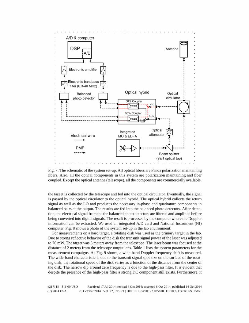
The system follows the schematic illustrated in Fig. 7. An integrated MO and EDFA config-uration generates a fiber coupled Gaussian beam at the wavelength of 1565 nm. The maximumoutput power is around 1.35 W. The output is split by an optical tap into two signals: LO andtransmit signals. The splitting ratio is 99/1; that is, 99% of the laser power is directed towardsthe telescope (via the optical circulator) while 1% of the power is fed into an optical attenuatorfor fine-tuning of the LO power. For optimal coherent detection the LO power should be largeenough so that the photo detectors are in shot-noise limited operation mode. However, it is im-perative to make sure the detectors are not operating in saturation mode. The return signal from


A/DDSP

Integrated

MO & EDFA

A/D & computer

Optical hybrid

Electronic bandpass

filter (0.3-40 MHz)

Electrical wire

PMF

50% Coupler

90 o

50% Coupler

Optical

circulatorBalanced

photo detector

Beam splitter

(99/1 optical tap)

Optical

attenuator

Electronic amplifier

Antenna

Fig. 7: The schematic of the system set-up. All optical fibers are Panda polarization maintainingfibers. Also, all the optical components in this system are polarization maintaining and fibercoupled. Except the optical antenna (telescope), all the components are commercially available.

the target is collected by the telescope and fed into the optical circulator. Eventually, the signalis passed by the optical circulator to the optical hybrid. The optical hybrid collects the returnsignal as well as the LO and produces the necessary in-phase and quadrature components inbalanced pairs at the output. The results are fed into the balanced photo detectors. After detec-tion, the electrical signal from the the balanced photo detectors are filtered and amplified beforebeing converted into digital signals. The result is processed by the computer where the Dopplerinformation can be extracted. We used an integrated A/D card and National Instrument (NI)computer. Fig. 8 shows a photo of the system set-up in the lab environment.

For measurements on a hard target, a rotating disk was used as the primary target in the lab.Due to strong reflective behavior of the disk the transmit signal power of the laser was adjustedto 70 mW. The target was 5 meters away from the telescope. The laser beam was focused at thedistance of 2 meters from the telescope output lens. Table 1 lists the system parameters for themeasurement campaigns. As Fig. 9 shows, a wide-band Doppler frequency shift is measured.The wide-band characteristic is due to the transmit signal spot size on the surface of the rotat-ing disk; the rotational speed of the disk varies as a function of the distance from the center ofthe disk. The narrow dip around zero frequency is due to the high-pass filter. It is evident thatdespite the presence of the high-pass filter a strong DC component still exists. Furthermore, it


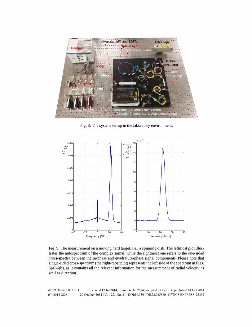
Fig. 8: The system set-up in the laboratory environment.

-40 -20 0 20 400

0.005

0.01

0.015

0.02

0.025

0.03

0.035

0 10 20 30 40-2

0

2

4

6

8

10

12

14

16x 10

-3

Frequency [MHz] Frequency [MHz]

Fig. 9: The measurement on a moving hard target, i.e., a spinning disk. The leftmost plot illus-trates the autospectrum of the complex signal, while the rightmost one refers to the one-sidedcross-spectra between the in-phase and quadrature-phase signal components. Please note thatsingle-sided cross-spectrum (the right-most plot) represents the left side of the spectrum in Figs.6(a)-6(b), as it contains all the relevant information for the measurement of radial velocity aswell as direction.


-40 -20 0 20 400

0.005

0.01

0.015

0.02

0.025

0.03

0.035

0 10 20 30 40-3

-2.5

-2

-1.5

-1

-0.5

0

0.5x 10

-3

Frequency [MHz] Frequency [MHz]

Fig. 10: The atmospheric measurement using the full output power of the laser. The measure-ment spectra is associated with the vertical component of the wind. The leftmost plot illus-trates the autospectrum of the complex signal, while the rightmost one refers to the one-sidedcross-spectra between the in-phase and quadrature-phase signal components. Please note thatsingle-sided cross-spectrum (the right-most plot) represents the left side of the spectrum in Figs.6(a)-6(b), as it contains all the relevant information for the measurement of radial velocity aswell as direction.

can be seen that the autospectrum, the leftmost plot in Fig. 9, exhibits a colored (filtered) Gaus-sian noise as expected across its frequency span. The filtering effect might become significantdue to environmental dependency of the electronic components. As a result, for the autospec-trum shown in the left-most plot in Fig. 9, noise whitening needs to be carried out before anaccurate radial speed can be estimated. The rightmost plot in Fig. 9 illustrates the one-sidedcross-spectral analysis, as a result of which the uncorrelated noise sources, e.g., shot noise, 1/fnoise, and DC noise due to reflections from the telescope, are suppressed. Besides, due to arelatively flat background spectrum, noise whitening is not required in this case. Thus, radialvelocity estimation is not only easier but also more accurate than the autospectral analysis forthe majority of scenarios.

Table 1: Experimental system parameters

Campaign pt [W] BW [MHz] fs [MHz] N M Aperture size [inches]

Hard target 70×10−3 40 120 512 4000 2Diffuse target 1.1 40 120 512 4000 2

For atmospheric measurements, the full output power of the integrated MO and EDFA was


used. Due to losses in the system (e.g., fiber connectors) the maximum output power to thetelescope was 1.1 W. Fig. 10 illustrates the atmospheric measurement. For this campaign thetelescope was pointing upward. As a result, the vertical component of the wind was measured.We know from experience that measuring the vertical component accurately is a challenge dueto the presence of the Doppler signal in the vicinity of the DC component (i.e., zero frequency).As seen in the leftmost plot in Fig. 10, the signal strength is much lower and the Doppler shift iscloser to zero. Accurate estimation of radial velocity in this case also requires additional signalprocessing and filtering. However, by utilizing the cross-spectral analysis, the majority of noisesources are suppressed and a rather flat spectra is achieved. It is evident that the benefits ofcross-spectral analysis are more emphasized for weaker Doppler signals and lower radial ve-locity speeds, where dilution with various noise sources around zero frequency is more severe.As we will show in a future paper, however, the merits of the cross-spectral technique becomequestionable once the Doppler spectrum crosses the zero frequency, where the signal containsboth negative and positive Doppler shifts close to zero.

5. Conclusion

By analyzing a promising new approach, an all-fiber image-reject architecture, for signal detec-tion in fiber CDLs, we have shown that a more robust system implementation can be realized.The robustness is partly the result of using passive components, as opposed to alternative sys-tem implementations such as heterodyne receivers that use active components, and partly at-tributable to a new approach in signal processing algorithm made available due to the presenceof in-phase and quadrature-phase signal components. Despite its simplicity, the signal process-ing algorithm, the cross-spectral analysis, improves the accuracy of Doppler shift estimationby eliminating the estimation inaccuracies often introduced by noise whitening procedure, aswell as suppressing the major extraneous noise present in the auto-spectral counter-part. Ad-ditionally, the presented system profits from a lower memory requirement for the storage ofthe estimated spectra. The new approach benefits from an all-fiber technology available in fiberoptic communications and is easy to implement.

Acknowledgments

The authors would like to thank Torben Mikkelsen, Mikael Sjoholm, Peter John Rodrigo, andChristophe Peucheret from Technical University of Denmark, as well as Mike Harris fromZephIR Lidar (UK), for the fruitful discussions that helped us understand the concepts moreclearly. This project is mainly funded by the WindScanner project from the Danish StrategicResearch Council, Danish Agency for Science -Technology and Innovation; Research Infras-tructure 2009; Grant No. 2136-08-0022. Ingeborg and Leo Dannin Grant for Scientific Researchfunded the NI computer used in this work.


an all-fiber image-reject homodyne coherent doppler wind...

Documents