an analysis of capital cost estimation techniques for chemical
TRANSCRIPT
An Analysis of Capital Cost Estimation Techniques for Chemical Processing
by
Omar Joel Symister
A thesis submitted to the Graduate School of
Florida Institute of Technology
in partial fulfillment of the requirements
for the degree of
Master of Science
in
Chemical Engineering
Melbourne, Florida
May, 2016
We, the undersigned committee, hereby approve the attached thesis, “An Analysis
of Capital Cost Estimation Techniques for Chemical Processing” by Omar Joel
Symister.
_________________________________________________
Jonathan Whitlow, Ph. D.
Major Advisor
Associate Professor of Chemical Engineering
College of Engineering
_________________________________________________
James Brenner, Ph. D.
Assistant Professor of Chemical Engineering
College of Engineering
_________________________________________________
Aldo Fabregas, Ph. D.
Assistant Professor, Engineering Systems
College of Engineering
_________________________________________________
Manolis Tomadakis, Ph. D.
Professor and Department Head, Chemical Engineering
College of Engineering
iii
Abstract
Title: An Analysis of Capital Cost Estimation Techniques for Chemical Processing
Author: Omar J. Symister
Advisor: Jonathan Whitlow, Ph. D.
This research serves to compare the use of the capital cost estimation software,
Aspen Capital Cost Estimator (ACCE), with other capital cost estimating methods
specifically the module costing technique outlined by Richard Turton et al. and also
a factorial costing technique outlined by Gavin Towler and Ray Sinnott. This study
will compare popular process equipment found in the chemical process industries.
The relationship between the capacities of the equipment, as it relates to the cost as
well as operational pressures and materials of construction (MOC), will also be
obtained and compared. The results of this study may be used by professionals in
their decision of which method of capital cost estimation they may want to employ.
The results and comparison varied a great deal based on the equipment being
costed, but for most of the equipment tested, the costs went up in a linear fashion.
For all of the methods studied, when the cost of the installed equipment is plotted
versus the capacity on a log-log scale a linear relationship is achieved. The slopes
of these lines (or capacity exponents) are presented in the work showing how the
economy of scale varies for the different cases studied. In general slopes of less
than unity are obtained with consistently different slope values for the three
methods. The ACCE usually had the lowest cost of the three methods. Another

iv
thing to note is that the factorial method had the least equipment data available,
while ACCE was the most diverse.

v
Table of Contents
Table of Contents ..................................................................................................... v
List of Figures ........................................................................................................ vii
List of Tables .......................................................................................................... ix
Acknowledgement .................................................................................................... x
Chapter 1 Introduction ............................................................................................ 1
Chapter 2 Objective of Study .................................................................................. 4
Chapter 3 Review of Literature .............................................................................. 5
Module Costing Method proposed by Turton et al. ..................................................... 7
Factorial Method proposed by Towler and Sinnott ..................................................... 8
Computer Program Use in Cost Estimation as evaluated by Ying Feng (2011) ...... 11
ASPEN Capital Cost Estimator (formerly AspenPEA) ............................................. 12
Chapter 4 Method of Research ............................................................................. 15
Process/Pressure Vessels ............................................................................................... 16
Other Process Equipment ............................................................................................. 17
Chapter 5 Results and Discussion ......................................................................... 18
Pressure Vessels ............................................................................................................. 19
Vertical Vessels .......................................................................................................... 19
Horizontal Vessels ...................................................................................................... 21
Heat Exchangers ............................................................................................................ 23
U-tube Shell and Tube ................................................................................................ 24
Floating Head .............................................................................................................. 26
vi
Kettle Reboiler ............................................................................................................ 28
Pumps and Drivers ........................................................................................................ 30
Centrifugal Pump ........................................................................................................ 30
Explosion Proof Motor ............................................................................................... 32
Compressors .................................................................................................................. 33
Centrifugal .................................................................................................................. 33
Reciprocating Compressors ........................................................................................ 35
Mixers ............................................................................................................................. 37
Propeller ...................................................................................................................... 37
Validation of Results ..................................................................................................... 38
Chapter 6 Conclusions and Recommendations ................................................... 41
References ............................................................................................................... 44
Appendix A Additional Equations used for Pressure Vessels ............................ 46
Appendix B The Aspen Capital Cost Estimator user interface ......................... 48
Appendix C ACCE Sample Item Report ............................................................. 51
vii
List of Figures
Figure 1: Cost vs. Capacity plot of a carbon steel vertical vessel at 1 bar ............... 20
Figure 2: Cost per unit capacity plot for a carbon steel vertical vessel at 1 bar....... 20
Figure 3: Cost per unit capacity plot for a stainless steel vertical vessel
at 1 bar .............................................................................................................. 21
Figure 4: Cost vs. Capacity plot of a carbon steel horizontal vessel at 1 bar........... 22
Figure 5: Cost per unit capacity plot for a carbon steel horizontal vessel
at 1 bar .............................................................................................................. 22
Figure 6: Cost per unit capacity plot for a stainless steel horizontal vessel
at 1 bar .............................................................................................................. 23
Figure 7: Cost vs. capacity plot for a carbon steel U-tube shell and tube heat
exchanger ......................................................................................................... 24
Figure 8: Cost per unit capacity plot for a carbon steel u-tube shell and tube
heat exchanger .................................................................................................. 24
Figure 9: Cost per unit capacity plot for a stainless steel u-tube shell and tube
heat exchanger .................................................................................................. 25
Figure 10: Cost vs. capacity plot of a carbon steel floating head shell and tube
heat exchanger .................................................................................................. 26
Figure 11: Cost per unit capacity plot for a carbon steel floating head
shell and tube heat exchanger .......................................................................... 27
Figure 12: Cost per unit capacity plot for a stainless steel floating head shell and
tube heat exchanger .......................................................................................... 27
Figure 13: Cost vs. capacity plot for a carbon steel U-tube kettle reboiler .............. 28
viii
Figure 14: Cost per unit capacity plot for a carbon steel U-tube kettle reboiler ...... 29
Figure 15: Cost per unit capacity plot for a stainless steel U-tube
kettle reboiler ................................................................................................... 29
Figure 16: Cost vs. capacity plot for a carbon steel centrifugal pump ..................... 30
Figure 17: Cost per unit capacity plot for a carbon steel centrifugal pump ............. 31
Figure 18: Cost per unit capacity plot for a stainless steel centrifugal pump .......... 31
Figure 19: Cost vs. capacity plot of a carbon steel explosion proof motor .............. 32
Figure 20: Cost per unit capacity plot for a carbon steel explosion proof motor .... 33
Figure 21: Cost vs. capacity plot for a carbon steel centrifugal compressor ........... 34
Figure 22: Cost per unit capacity plot for a carbon steel centrifugal
compressor ....................................................................................................... 34
Figure 23: Cost per unit capacity plot for a stainless steel centrifugal
compressor ....................................................................................................... 35
Figure 24: Cost vs. capacity plot of a carbon steel reciprocating compressor ......... 36
Figure 25: Cost per unit capacity plot for a carbon steel reciprocating
compressor ....................................................................................................... 36
Figure 26: Cost vs. capacity plot of a carbon steel vertical propeller mixer ............ 37
Figure 27: Cost per unit capacity plot for a carbon steel propeller mixer ............... 38
Figure 28: Geneal project data window ................................................................... 48
Figure 29: Project component selection window ..................................................... 49
Figure 30: Equipment specification screen .............................................................. 50
ix
List of Tables
Table 1: Cost estimate classification matrix for process industries .......................... 2
Table 2: A summary of the cost exponents obtained for each method .................... 42
x
Acknowledgement
I would like to thank my family and friends for their never ending support and
encouragement. I give a special thanks to my father, who always challenges me to
do my very best. I would also like to thank the faculty in the Chemical Engineering
Department, as well as Dr. Fabregas from Engineering Systems, for the continued
support, guidance, and patience during this endeavor.
1
Chapter 1
Introduction
According to Perry’s Chemical Engineering Handbook 1, the total capital
investment includes funds required to purchase land, design and purchase
equipment, structures, and buildings, as well as to bring them into operation. This
may be a daunting task for the cost engineer depending on the scope and size of the
process being built. This study aims to compare different methods of calculating
the equipment capital cost for major process equipment found inside many process
plants. Furthermore, a comparison to Aspen Capital Cost Estimation (ACCE)
software package will be done as well.
A major factor in deciding whether or not to build or expand any chemical/process
plant is the capital cost estimation. The capital cost is the investment that is put in
to build or expand the plant. During the design process, it is nearly impossible to
know the exact quantity of this investment. This is why it is important for the
engineers and project managers to get as close to the actual value as possible.
Usually, methods proposed by authors have bases from correlations of actual
vendor data. Couper et al. mentions that there will be a certain amount of scatter in
price data. This may be due to variations among manufacturers, quality of
construction among other factors. The authors continue to say that the accuracy of
the correlations cannot be better than ± 25% 2. The methods below shall be used in
study estimates.
2
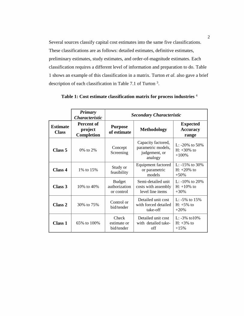
Several sources classify capital cost estimates into the same five classifications.
These classifications are as follows: detailed estimates, definitive estimates,
preliminary estimates, study estimates, and order-of-magnitude estimates. Each
classification requires a different level of information and preparation to do. Table
1 shows an example of this classification in a matrix. Turton et al. also gave a brief
description of each classification in Table 7.1 of Turton 3.
Table 1: Cost estimate classification matrix for process industries 4
Primary
Characteristic Secondary Characteristic
Estimate
Class
Percent of
project
Completion
Purpose
of estimate Methodology
Expected
Accuracy
range
Class 5 0% to 2% Concept
Screening
Capacity factored,
parametric models,
judgement, or
analogy
L: -20% to 50%
H: +30% to
+100%
Class 4 1% to 15% Study or
feasibility
Equipment factored
or parametric
models
L: -15% to 30%
H: +20% to
+50%
Class 3 10% to 40%
Budget
authorization
or control
Semi-detailed unit
costs with assembly
level line items
L: -10% to 20%
H: +10% to
+30%
Class 2 30% to 75% Control or
bid/tender
Detailed unit cost
with forced detailed
take-off
L: -5% to 15%
H: +5% to
+20%
Class 1 65% to 100%
Check
estimate or
bid/tender
Detailed unit cost
with detailed take-
off
L: -3% to10%
H: +3% to
+15%

3
According to AACE International, process technology, cost data, and many other
risks affect the accuracy range. The range typically represents a 50% confidence
interval4.
Order-of-magnitude estimates usually rely on cost information for a complete
process. This information is usually taken from previously built plants. This cost
information is scaled using scaling factors for capacity and inflation. This estimate
is also called the ratio or feasibility estimate and usually requires a block flow
diagram.
Moving along in increasing order of complexity and detail is the study estimate.
The study estimate uses a list of the major equipment included in the process, such
as pumps, compressors and turbines, columns and vessels, heat exchangers, etc.
After sizing is done, the cost is determined for each piece of equipment. Also called
the major equipment or factored estimate, the study estimate usually needs cost
charts and process flow diagrams 3. Only these two estimates will be looked at for
the most part in this thesis.
4
Chapter 2
Objective of Study
The objective of this research is to compare the use of the capital cost estimation
software, Aspen Plus Capital Cost Estimator (ACCE), with methods proposed by
Turton et al. 3 and also Towler and Sinott 5. Using these methods, this study
compares the capital costs of ten types of equipment, including various types of
mixers, pumps, heat exchangers, compressors, and pressure vessels. The equipment
type chosen was limited to those common to each of the three methods. The
relationship between the capacities of the equipment as it relates to the cost as well
as operational pressures and materials of construction (MOC) was obtained and
compared where possible.
Equipment Scope – equipment supported by all three methods was:
• Mixers: Propeller
• Compressors: Centrifugal; Reciprocating
• Exchangers: U-tube shell and tube; Floating head shell and tube; U-tube
kettle reboiler
• Pressure Vessels: Vertical; Horizontal
• Pumps and Drivers: Single stage centrifugal; Explosion proof motor
5
Chapter 3
Review of Literature
Although the most accurate way to estimate the purchase cost of a piece of
equipment is to get a current price quote from the appropriate vendor, this may
sometimes prove difficult to obtain based on the vendor's policies. The next best
alternative would be to use cost data from previously purchased equipment of the
same type. Based on previous cost data, the current cost of equipment could change
based on differences in the equipment capacity and also differences in time.3
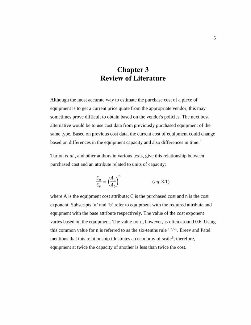
Turton et al., and other authors in various texts, give this relationship between
purchased cost and an attribute related to units of capacity:
𝐶𝑎
𝐶𝑏= (
𝐴𝑎
𝐴𝑏)
𝑛
(𝑒𝑞. 3.1)
where A is the equipment cost attribute; C is the purchased cost and n is the cost
exponent. Subscripts ‘a’ and ‘b’ refer to equipment with the required attribute and
equipment with the base attribute respectively. The value of the cost exponent
varies based on the equipment. The value for n, however, is often around 0.6. Using
this common value for n is referred to as the six-tenths rule 1,3,5,6. Ereev and Patel
mentions that this relationship illustrates an economy of scale6; therefore,
equipment at twice the capacity of another is less than twice the cost.
6
If cost data is collected from previous years, the cost forecast for current year and
years to come will be different due to factors such as inflation. To account for this
change, cost indexes are used. Turton also gives the following relationship:
𝐶2 = 𝐶2 (𝐼2
𝐼1) (𝑒𝑞. 3.2)
where C is the purchased cost, I is the cost index. 1 and 2 refer to the base time
when cost is known and the time when cost is desired, respectively.
There are several indices used in the chemical industry to adjust for inflation. These
include:
The Nelson-Farrar Refinery Index 7,8
The Marshall and Swift (M&S) Index 8
The Engineering News – Record Construction Index 8,9
The Chemical Engineering Plant Cost Index (CEPCI) 8,10
Turton uses CEPCI to account for inflation in the literature.
Turton et al. also covers the total capital cost of a plant. The authors go through
methods of calculating the total module cost (total capital cost), such as the Lang
factor technique 3,5,11 and the module costing technique.
For the Lang factor technique, the total capital cost is determined by the product of
the total purchased cost and a constant known as the Lang factor. The equation is as
follows:
7
𝐶𝑇𝑀 = 𝐹𝐿𝑎𝑛𝑔 ∑ 𝐶𝑝,𝑖
𝑛
𝑖=1
(𝑒𝑞. 3.3)
where CTM is the capital cost of the plant; Cp,i is the purchased cost of the major
equipment units; n is the total number of units and FLang is the appropriate Lang
factor.
The Lang factor is given in Turton for three types of chemical plants – plants that
process only fluids (FLang = 4.74); plants that process only solids (FLang = 3.10); and
plants that process both solids and liquids (FLang = 3.63).
This technique, unfortunately, does not account for special changes in the process
such as materials of construction and high operating pressures.
Module Costing Method proposed by Turton et al.
The module costing technique, however, does factor in these changes based on
specific equipment type, system pressure and materials of construction.
Equation 3.4 is used to calculate the bare module cost which is the sum of the direct
and indirect costs. Direct costs entail the equipment free on board (f.o.b.) cost and
the materials required for installation (piping, insulation and fireproofing,
foundations and structural supports, instrumentation and electrical, and painting)
and also the labor to install equipment and material. Indirect costs entail freight,
insurance, taxes, construction overhead, and contractor engineering expenses.
𝐶𝐵𝑀 = 𝐶𝑝0𝐹𝐵𝑀 (𝑒𝑞. 3.4)
where CBM is the bare module equipment cost; FBM is the bare module cost factor
(looked up in tables in the appendix of Turton's text) that is based on material of
construction and operating pressure; C0p is the purchased cost for base conditions
8
(common materials and near-ambient pressures). In order to incorporate the
equipment material and pressure, a modification to the equation above can be used.
Equation 3.5 adds additional constants such as a material factor (FM) and a pressure
factor (FP) (see equations A.3 and A.5). From correlations, the constants B1 and B2
are material specific and may be found in tables in Turton.
𝐶𝐵𝑀 = 𝐶𝑝0𝐹𝐵𝑀 = 𝐶𝑝
0(𝐵1 + 𝐵2𝐹𝑀𝐹𝑃) (𝑒𝑞. 3.5)
Furthermore, the data for the purchased cost of equipment, at ambient temperature
and using carbon steel, were fitted to the following equation:
log(𝐶𝑝0) = 𝐾1 + 𝐾2 log(𝐴) + 𝐾3[log(𝐴)]2 (𝑒𝑞. 3.6)
where K1, K2 and K3 are equipment specific constants also found in the appendix of
Turton.
Turton’s method does not offer much flexibility for calculating just a direct cost or
indirect cost as with the factorial method. Material, labor and installation costs as a
function of other factors are given, but actual values for these factors are not given.
Another thing to note about the data in Turton is that they are based on a survey of
equipment manufacturers during May to September of 2001. The average CEPCI
value during this period was 397. According to Turton et al., this method was first
proposed by Guthrie and modified by Ulrich 3.
Factorial Method proposed by Towler and Sinnott
In Towler and Sinnott, the Fixed Capital Investment (FCI) is given as an inside
battery limits (ISBL) – which is the cost of the plant itself including:
Equipment purchase cost
9
Equipment erection, including foundations and minor structural work
Piping, including insulation and painting
Electrical, power and lighting
Instruments and automatic process control (APC) systems
Site preparations
Also, the FCI consists of the outside battery limits (OSBL), the construction and
engineering costs, offsites and contingency charges (not studied in this thesis).
Towler and Sinnott agree with Turton et al. when it comes down to the
classification of cost estimates as both literature sources used the classifications put
forward by the Association for the Advancement of Cost Estimating4 (AACE
Intenational, see Table 1). They also agree on how one goes about doing the order-
of-magnitude calculations for changes in capacity [equation (3.1)].
Towler and Sinnott, however, puts forward a different correlation in order to
calculate purchased equipment costs. These correlations are in the form of the
following equation.
𝐶𝑒 = 𝑎 + 𝑏𝑆𝑛 (𝑒𝑞. 3.7)
where Ce is the purchased equipment cost; a and b are constants found in Table 7.2
in Towler and Sinnott5, S is the size parameter, and n is the exponent for that type
of equipment.
The purchased equipment cost uses a US Gulf Coast basis in January 2010. This
period has a CEPCI of 532.9 and a NF refinery index of 2281.6. Prices are all for
10
carbon steel. Towler and Sinnott also mentioned that this method is more for a
preliminary design estimate.
For more detailed estimates that account for the type of material used other than
carbon steel and also installation costs (CISBL), Towler and Sinnott uses what is
called the Factorial Method. The CISBL is somewhat similar to the CBM. The CISBL
used in Towler and Sinnott is a direct cost, whereas CBM has direct and indirect.
This is calculated using an expansion of the Lang factor equation:
𝐶 = ∑ 𝐶𝑒,𝑖,𝐶𝑆[(1 + 𝑓𝑝)𝑓𝑚 + (𝑓𝑒𝑟 + 𝑓𝑒𝑙 + 𝑓𝑖 + 𝑓𝑐 + 𝑓𝑠 + 𝑓𝑙)]
𝑖=𝑀
𝑖=1
(𝑒𝑞. 3.8)
This equation should be used when the purchase cost has been found on a carbon
steel basis. If found on a basis other than carbon steel, the following equation
should be used with the installation factors corrected.
𝐶 = ∑ 𝐶𝑒,𝑖,𝐴[(1 + 𝑓𝑝) + (𝑓𝑒𝑟 + 𝑓𝑒𝑙 + 𝑓𝑖 + 𝑓𝑐 + 𝑓𝑠 + 𝑓𝑙)/𝑓𝑚]
𝑖=𝑀
𝑖=1
(𝑒𝑞. 3.9)
where Ce,i,CS is the purchased equipment cost of equipment i in carbon steel, Ce,i,A is
the purchased equipment cost of equipment i in alloy, M is the total number of
pieces of equipment. The other factors are for piping (fp), equipment erection (fer),
electrical, instrumentation and control (fi), civil engineering work (fc), structures
and buildings (fs), lagging, insulation and paint (fl) and a materials factor (fm)5.
The list of process equipment information Towler and Sinnott is not as diverse as
the one given in Turton and does not account for different design pressures or type
of equipment.
11
Computer Program Use in Cost Estimation as evaluated
by Ying Feng (2011)
An article published in the August 2011 edition of Chemical Engineering Journal
by Feng and Rangaigh compares five capital cost estimation programs. Some of
these programs use the same methods proposed by authors in the texts covered
above. The five programs evaluated were as follows: CapCost, EconExpert,
AspenTech Process Economic Analyzer (Aspen Tech PEA), Detailed Factorial
Program (DFP), and Capital Cost Estimation Program (CCEP). The authors used
case studies to evaluate the five programs at the equipment and plant levels.
The first program evaluated was CapCost. This program uses the module costing
method as discussed in Turton et al. This is available with the process design book
written by Turton et al.; furthermore, the program is written in Visual Basic and is
able to handle preliminary process cost. The second program evaluated by Feng is
the Detailed Factorial Program (DFP). This program uses the detailed factorial
estimate as laid out in the book by Towler and Sinott. However, in the article, the
constants correspond to a January 2007 CEPCI of 509.7 (instead of 532.9 in 2010
as discussed above).
The third program was Capital Cost Estimating Program (CCEP). This used a
correlation presented in Seider 11 for estimation of free on board (FOB) cost of
equipment. According to Feng, Seider developed these purchased cost correlations
for common process equipment based on available literature sources and vendor
data. The program also uses material factors and Guthrie’s bare module factors
thereafter to estimate equipment costs. These correlations may be found in the book
written by Seider et al. using a CEPCI of 500 (2006 average). The equation used
for is similar to the equation used by Turton et al. to calculate C0p:
12
𝐶𝑝0 = exp{𝐴1 + 𝐴2 𝑙𝑜𝑔(𝑆) + 𝐴3[𝑙𝑜𝑔(𝑆)]2 + ⋯ } (𝑒𝑞. 3.10)
EconExpert is the fourth program evaluated. According to Feng, it is a Web-based
interactive software for capital cost estimation 12. It also uses the equipment module
costing method. The data for this program may be found in “Chemical Engineering
Process Design and Economics by Ulrich and Vasudevan 12. Ulrich and Vasudevan
present the data in plots and graphs. EconExpert represents these plots in
polynomial form using multiple regression. EconExpert uses a CEPCI of 400 (2002
average).
The last program is AspenPEA (predecessor to ACCE), which is designed to
generate both conceptual and detailed estimates. AspenPEA claims to have time-
proven, field tested, industry-standard cost modeling and scheduling methods. Feng
used AspenPEA version 7.1, which follows 2008 data with a CEPCI of 575.
This article covered an adequate amount of process equipment including
compressors, heat exchangers, mixers, pumps, towers, and vessels among others.
Also covered were the total purchase and module costs. Feng found that all
programs were user-friendly. The author also found that AspenPEA had the most
equipment types available, while DFP was the most limited. Furthermore, the
overall plant cost does not differ by much; however, the programs differed
significantly for the equipment costs. This wasn’t the case for all equipment, but for
certain equipment types.12
ASPEN Capital Cost Estimator (formerly AspenPEA)
Economics in Aspen involves two software systems: The process simulator (Aspen
Plus) and the economic evaluation software (Aspen Capital Cost Estimator13). Both
are integrated by having the economics software embedded in the process
simulator. Aspen Capital Cost Estimator (ACCE) is a model-based estimator
13
which, according to AspenTech, employs a sophisticated “volumetric model” rather
than a factor-based model as discussed earlier. ACCE uses cost models to prepare
detailed lists of costs of process equipment and bulk materials. AspenTech claims
that these models have been tested and improved over time with feedback from
organizations that use the ACCE 14,15. However, obtaining the actual model or data
used to come up with this model isn’t easy due to Aspen Plus being a proprietary
software. ACCE v8.8 uses a 1st Qtr. 2014 pricing basis (CEPCI 576.1).
The pricing changes in Aspen Icarus Evaluation Engine for V8.6 (2013 basis) to
V8.8 may be found in the help menu of the software16. The changes included:
a 2.7% decrease to a 0.8% increase in equipment costs
a 3.3% decrease to a 5.6% increase in piping costs
a 0% to 4.4% increase in civil engineering costs
a 1.3% decrease to a 3% increase in steel costs
a 7.5% to 13.8% increase in instrumentation costs
a 0.3% to 2.3% decrease in electrical costs
a 3.1% decrease to 1.7% increase in insulation costs
a 0.5% to 0.9% increase in paint costs
Carbon steel plate pricing had an approx. 8% increase
304 stainless steel plate pricing had an approx. 2% decrease while tubing
had a 17% decrease
14
Some changes shown were dependent on location. According to the software,
“these results were obtained by running a general benchmark project containing a
representative mix of equipment found in a gas processing plant. In addition to
pricing changes, model enhancements and defect corrections have affected overall
percentage differences.”16 The software also noted, “…the costs may include
quantity or design differences, since various models and methods have been
updated or fine-tuned based on client feedback and defect resolution.”16
15
Chapter 4
Method of Research
This study employed the use of the Aspen Capital Cost Estimator (ACCE) to
evaluate the equipment used in the study. Aspen Plus Process Simulator also has
the ability to estimate capital costs based on these simulated processes using what
is called Active Economics. Active Economics ultimately uses the ACCE to do
this. By using ACCE directly, the dependency on which raw materials are used as
inputs in the process is eliminated. The cost of each piece of equipment, at each
scenario, was estimated using Turton’s Module Costing Method (first proposed by
Guthrie and modified by Ulrich), Towler and Sinnott’s Factorial Method (assumed
a fluids processing plant), and using the ACCE. Calculations outside of Aspen
were done using Excel. Using these tools, a comparison of equipment capital costs
was made among these different techniques. Furthermore, feasible capacity ranges
(low, middle, high) and materials of construction (carbon steel and 304 stainless
steel) were modified and compared for each piece of equipment looked at in this
study. All final costs are brought to 2014 final values by the use of the Chemical
Engineering Plant Cost Index (CEPCI) obtained from the Chemical Engineering
Magazine. For a look at the ACCE user interface and a general procedure, see
Appendix B. However, for a detailed description of how to use the ACCE software,
refer to the user guide13.
16
Process/Pressure Vessels
For the vertical pressure vessels, the capacities chosen were based on feasible
ranges laid out in the methods studied. Each method also required different
specifications. For a list of additional equations used for the pressure vessels, see
Appendix A. For Turton’s method, the capacity ranges are from 0.3 to 520 m3. For
Towler and Sinnott, the capacity ranged from 160 to 250,000 kg of shell mass.
ACCE was more flexible and required either the diameter with the tangent to
tangent height, or just the liquid volume. The former option was used in Aspen.
With these constraints in place, it was decided to keep the diameter fixed at 3
meters and change only the length of the vessel. Lengths between 10 and 30 meters
suited both feasibility ranges resulting in volumes between 70 and 212 m3 (see
equation A.4). Furthermore, this also resulted in shell masses ranging between
8,800 and 36,000 kg by using the densities of carbon or stainless steel where
applicable (see equation A.2). A high and a low design pressure were chosen
between feasibility ranges laid out in Turton. In this case, the low pressure was 1
bar, and the high was 10 bar. In the case of Towler and Sinnott’s method, which
does not account for pressure in the cost equations, the wall thickness was used
based on the pressure chosen (equation A.1). This circumvents that problem as wall
thickness is a function of pressure. The wall thickness is also needed to find a shell
mass. This study also assumed an operating temperature of 30 degrees Celsius.
This assumption is needed due to the maximum allowable stress for stainless steel
decreasing as temperature increases. A weld efficiency, which also affects the wall
thickness, was assumed to be 100% for simplicity. For horizontal vessels, the
lengths chosen to meet the constraints were between 1 and 4 meters.
17
Other Process Equipment
The three heat exchangers chosen were treated the same, except for the capacity
ranges. The U-tube and floating head shell and tube heat exchangers had capacities
between 50 and 1000 m2; whereas, the U-tube kettle reboiler had capacities of 15
and 100 m2. The shell and tube sides were either CS/CS or SS/SS, and the pressures
were the same on both sides as well.
The pumps and compressors were sized in Aspen Plus v8.8 in order to obtain the
different capacities requirements for each method to get as best a comparison as
possible. For example, the pump capacity in Towler and Sinnott’s method requires
a flow rate while Turton’s method requires a shaft power; so, in order to make sure
the same specification pump is being costed, a flow rate and a pressure increase
was specified in the process simulator using water at 25oC and 1 bar as the input.
After the simulation is complete, the design pressure and head required can also be
specified along with the flow and power into the ACCE.
For the compressors, a little mathematical manipulation was necessary to obtain a
fluid power to be used with Turton’s method (see equation 4.1).
𝐹𝑙𝑢𝑖𝑑 𝑃𝑜𝑤𝑒𝑟(𝑘𝑊) = 𝐵𝑟𝑎𝑘𝑒 𝑃𝑜𝑤𝑒𝑟 (𝑘𝑊) ∗ 𝐸𝑓𝑓𝑖𝑐𝑖𝑒𝑛𝑐𝑦 (4.1)
An efficiency of 78% suggested by table 11.10 of Turton3 was used . Towler and
Sinnotts’s method used brake power as the capacity. An inlet flow was specified in
Aspen.
Mixers and motors were costed as outlined in Towler and Sinnott and Turton. For
mixers, the range chosen was between 5 and 75 kW; for the explosion proof motor
a range of 200 to 2500 kW was chosen.
18
Chapter 5
Results and Discussion
By linearizing the six-tenths rule (equation 3.1), one gets equation 5.1 below.
log(𝐶𝑎) = 𝑛𝑙𝑜𝑔(𝐴𝑎) + k (5.1)
where the constant ‘k’ is log(𝐶𝑏 𝐴𝑏𝑛⁄ ). According to Perry, the data is most accurate
in the narrow middle range of capacity, and that the error is large at both ends of
capacity (high or low) 1. Table 9-50 in Perry’s Chemical Engineering Handbook17
has a list of cost data which includes the exponent for various pieces of equipment.
When compared to ACCE, Towler and Sinnott’s method was generally the highest
of the two other methods, with exceptions in some cases. This may be due to each
method including different contributors to cost and also how these contributors are
accounted for. As for Towler and Sinnott’s factorial method, which covers only the
direct capital cost and also site preparation, the percent differences were about the
same for carbon steel and stainless steel values, which shows the errors are
consistent between the two methods.
Stainless steel is approximately four times more expensive than steel according to
MEPS International – an independent supplier of steel market information and
trends18; so it is expected to see an increase in price going from carbon steel to
stainless steel. All three methods are consistent with their costs.
As capacity increases there is an economy of scale displayed in the results. Looking
at the cost per unit capacity graphs below, one can see that as capacity increases,
19
the price per unit decreases, and in some cases the cost per unit capacity actually
starts to increase again.
If the design pressure increases, then the design engineer would have to make
adjustments accordingly, especially for wall thickness. Increasing the wall
thickness for the vessels would, intuitively, increase the amount of material needed
to fabricate the vessels and increase its cost. This is also reflected in the results for
each process vessel. The cost exponents obtained for the elevated pressures were
similar.
Pressure Vessels
Vertical Vessels
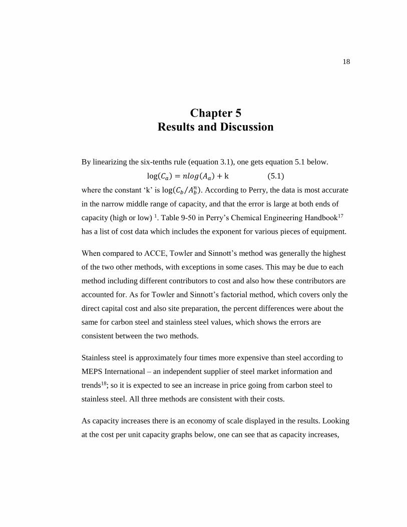
The exponents obtained for the vertical pressure vessels were n = 0.90, 0.76, 0.60
for Turton’s Method, Towler & Sinnott’s method and ACCE, respectively.
Observation of Figure 1 shows that the points behaved well in this range for the
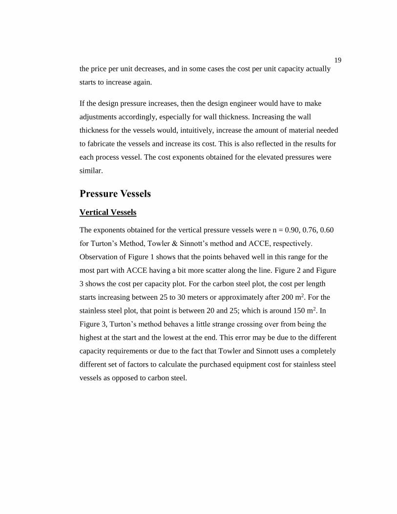
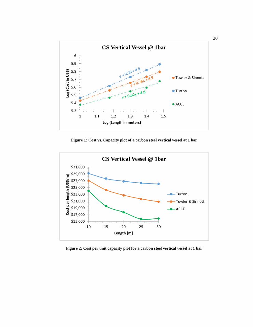
most part with ACCE having a bit more scatter along the line. Figure 2 and Figure
3 shows the cost per capacity plot. For the carbon steel plot, the cost per length
starts increasing between 25 to 30 meters or approximately after 200 m2. For the
stainless steel plot, that point is between 20 and 25; which is around 150 m2. In
Figure 3, Turton’s method behaves a little strange crossing over from being the
highest at the start and the lowest at the end. This error may be due to the different
capacity requirements or due to the fact that Towler and Sinnott uses a completely
different set of factors to calculate the purchased equipment cost for stainless steel
vessels as opposed to carbon steel.
20
Figure 1: Cost vs. Capacity plot of a carbon steel vertical vessel at 1 bar
Figure 2: Cost per unit capacity plot for a carbon steel vertical vessel at 1 bar
5.3
5.4
5.5
5.6
5.7
5.8
5.9
6
1 1.1 1.2 1.3 1.4 1.5
Log
(Co
st in
US$
)
Log (Length in meters)
CS Vertical Vessel @ 1bar
Towler & Sinnott
Turton
ACCE
$15,000
$17,000
$19,000
$21,000
$23,000
$25,000
$27,000
$29,000
$31,000
10 15 20 25 30
Co
st p
er
len
gth
[U
S$/m
]
Length [m]
CS Vertical Vessel @ 1bar
Turton
Towler & Sinnott
ACCE
21
Figure 3: Cost per unit capacity plot for a stainless steel vertical vessel at 1 bar
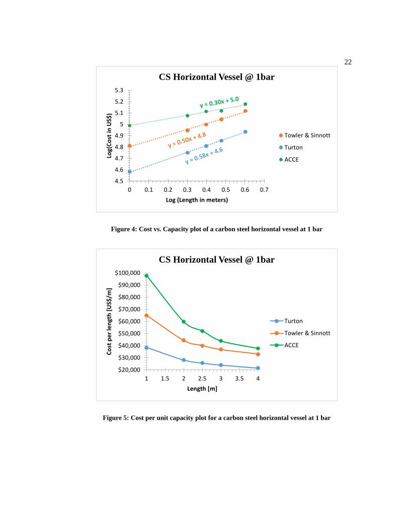
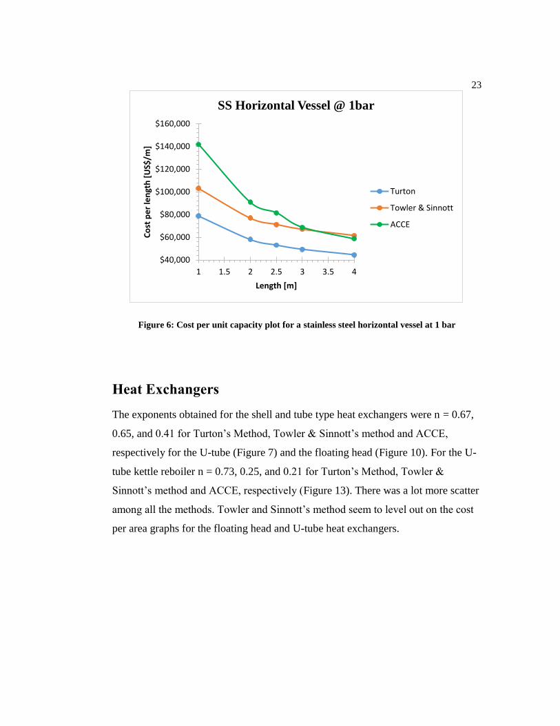
Horizontal Vessels
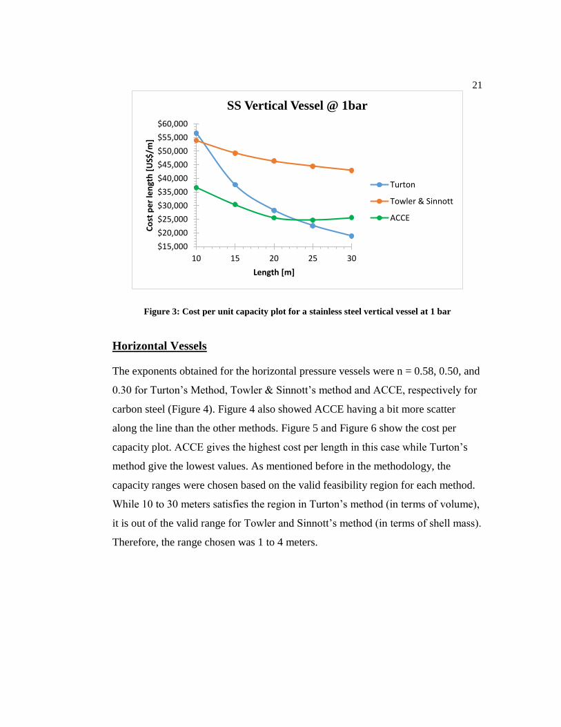
The exponents obtained for the horizontal pressure vessels were n = 0.58, 0.50, and
0.30 for Turton’s Method, Towler & Sinnott’s method and ACCE, respectively for
carbon steel (Figure 4). Figure 4 also showed ACCE having a bit more scatter
along the line than the other methods. Figure 5 and Figure 6 show the cost per
capacity plot. ACCE gives the highest cost per length in this case while Turton’s
method give the lowest values. As mentioned before in the methodology, the
capacity ranges were chosen based on the valid feasibility region for each method.
While 10 to 30 meters satisfies the region in Turton’s method (in terms of volume),
it is out of the valid range for Towler and Sinnott’s method (in terms of shell mass).
Therefore, the range chosen was 1 to 4 meters.
$15,000
$20,000
$25,000
$30,000
$35,000
$40,000
$45,000
$50,000
$55,000
$60,000
10 15 20 25 30
Co
st p
er
len
gth
[U
S$/m
]
Length [m]
SS Vertical Vessel @ 1bar
Turton
Towler & Sinnott
ACCE
22
Figure 4: Cost vs. Capacity plot of a carbon steel horizontal vessel at 1 bar
Figure 5: Cost per unit capacity plot for a carbon steel horizontal vessel at 1 bar
4.5
4.6
4.7
4.8
4.9
5
5.1
5.2
5.3
0 0.1 0.2 0.3 0.4 0.5 0.6 0.7
Log(
Co
st in
US$
)
Log (Length in meters)
CS Horizontal Vessel @ 1bar
Towler & Sinnott
Turton
ACCE
$20,000
$30,000
$40,000
$50,000
$60,000
$70,000
$80,000
$90,000
$100,000
1 1.5 2 2.5 3 3.5 4
Co
st p
er
len
gth
[U
S$/m
]
Length [m]
CS Horizontal Vessel @ 1bar
Turton
Towler & Sinnott
ACCE
23
Figure 6: Cost per unit capacity plot for a stainless steel horizontal vessel at 1 bar
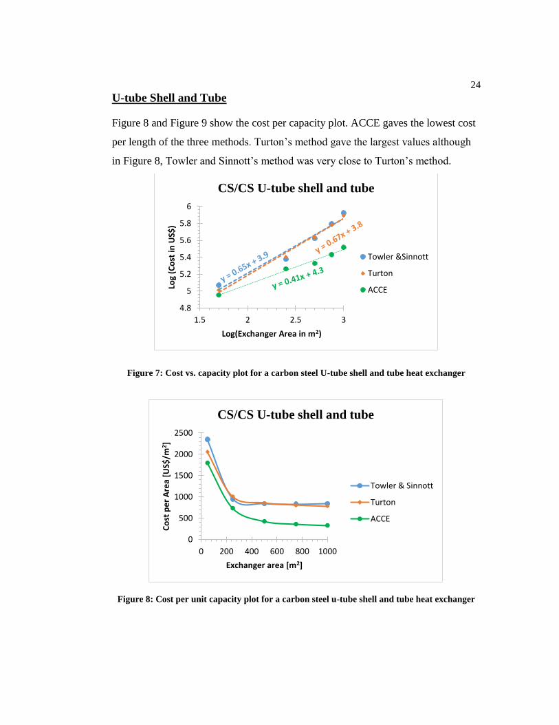
Heat Exchangers
The exponents obtained for the shell and tube type heat exchangers were n = 0.67,
0.65, and 0.41 for Turton’s Method, Towler & Sinnott’s method and ACCE,
respectively for the U-tube (Figure 7) and the floating head (Figure 10). For the U-
tube kettle reboiler n = 0.73, 0.25, and 0.21 for Turton’s Method, Towler &
Sinnott’s method and ACCE, respectively (Figure 13). There was a lot more scatter
among all the methods. Towler and Sinnott’s method seem to level out on the cost
per area graphs for the floating head and U-tube heat exchangers.
$40,000
$60,000
$80,000
$100,000
$120,000
$140,000
$160,000
1 1.5 2 2.5 3 3.5 4
Co
st p
er
len
gth
[U
S$/m
]
Length [m]
SS Horizontal Vessel @ 1bar
Turton
Towler & Sinnott
ACCE
24
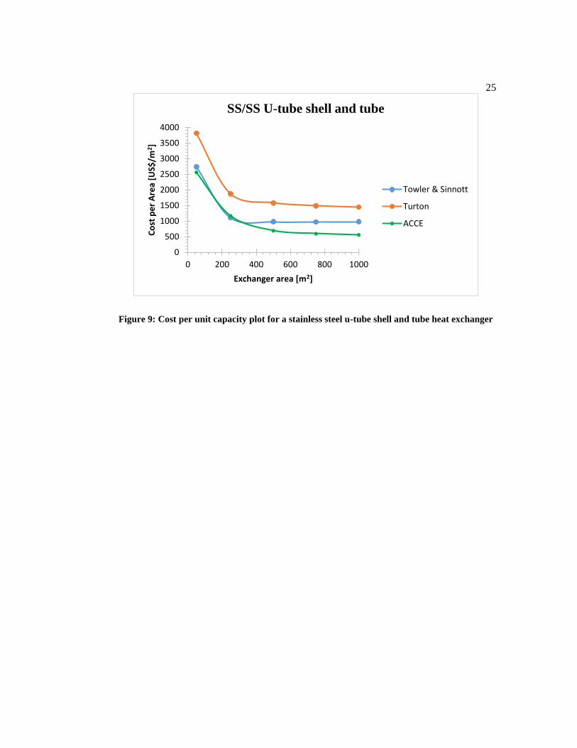
U-tube Shell and Tube
Figure 8 and Figure 9 show the cost per capacity plot. ACCE gaves the lowest cost
per length of the three methods. Turton’s method gave the largest values although
in Figure 8, Towler and Sinnott’s method was very close to Turton’s method.
Figure 7: Cost vs. capacity plot for a carbon steel U-tube shell and tube heat exchanger
Figure 8: Cost per unit capacity plot for a carbon steel u-tube shell and tube heat exchanger
4.8
5
5.2
5.4
5.6
5.8
6
1.5 2 2.5 3
Log
(Co
st in
US$
)
Log(Exchanger Area in m2)
CS/CS U-tube shell and tube
Towler &Sinnott
Turton
ACCE
0
500
1000
1500
2000
2500
0 200 400 600 800 1000
Co
st p
er
Are
a [U
S$/m
2 ]
Exchanger area [m2]
CS/CS U-tube shell and tube
Towler & Sinnott
Turton
ACCE
25
Figure 9: Cost per unit capacity plot for a stainless steel u-tube shell and tube heat exchanger
0
500
1000
1500
2000
2500
3000
3500
4000
0 200 400 600 800 1000
Co
st p
er
Are
a [U
S$/m
2 ]
Exchanger area [m2]
SS/SS U-tube shell and tube
Towler & Sinnott
Turton
ACCE
26
Floating Head
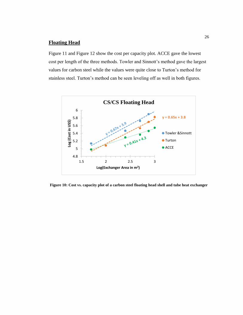
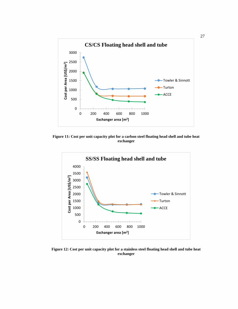
Figure 11 and Figure 12 show the cost per capacity plot. ACCE gave the lowest
cost per length of the three methods. Towler and Sinnott’s method gave the largest
values for carbon steel while the values were quite close to Turton’s method for
stainless steel. Turton’s method can be seen leveling off as well in both figures.
Figure 10: Cost vs. capacity plot of a carbon steel floating head shell and tube heat exchanger
y = 0.65x + 3.8
4.8
5
5.2
5.4
5.6
5.8
6
1.5 2 2.5 3
Log
(Co
st in
US$
)
Log(Exchanger Area in m2)
CS/CS Floating Head
Towler &Sinnott
Turton
ACCE
27
Figure 11: Cost per unit capacity plot for a carbon steel floating head shell and tube heat
exchanger
Figure 12: Cost per unit capacity plot for a stainless steel floating head shell and tube heat
exchanger
0
500
1000
1500
2000
2500
3000
0 200 400 600 800 1000
Co
st p
er
Are
a [U
S$/m
2 ]
Exchanger area [m2]
CS/CS Floating head shell and tube
Towler & Sinnott
Turton
ACCE
0
500
1000
1500
2000
2500
3000
3500
4000
0 200 400 600 800 1000
Co
st p
er
Are
a [U
S$/m
2 ]
Exchanger area [m2]
SS/SS Floating head shell and tube
Towler & Sinnott
Turton
ACCE
28
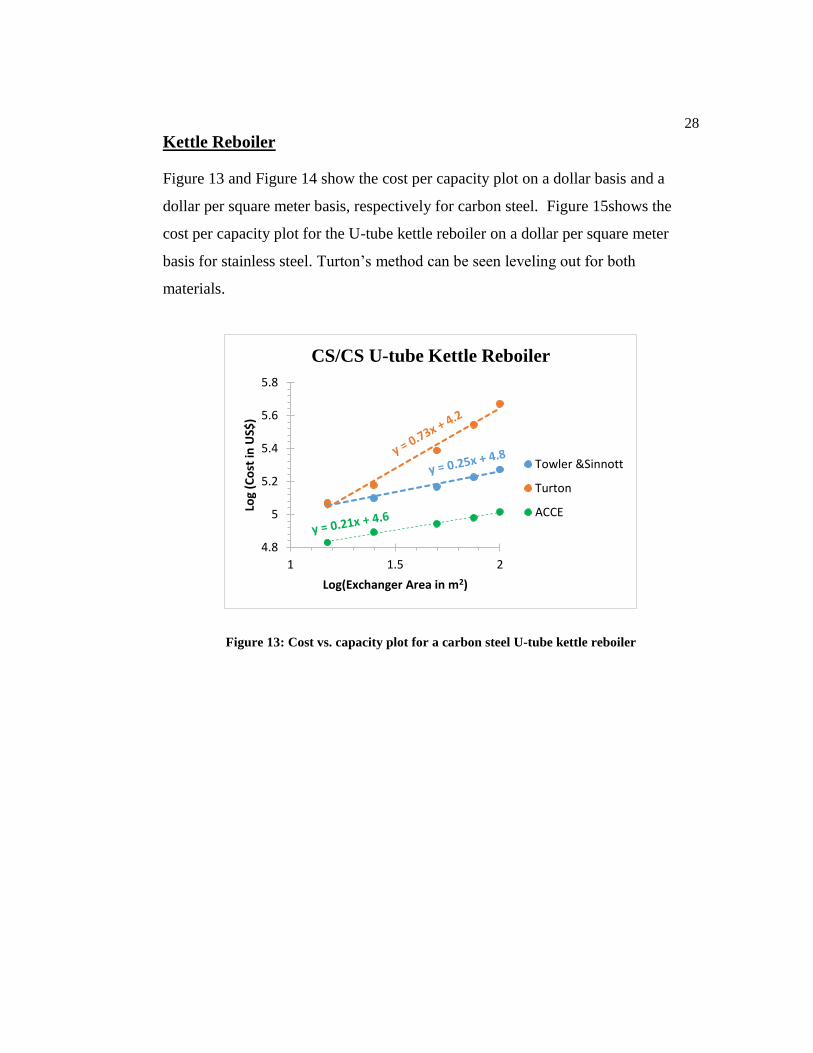
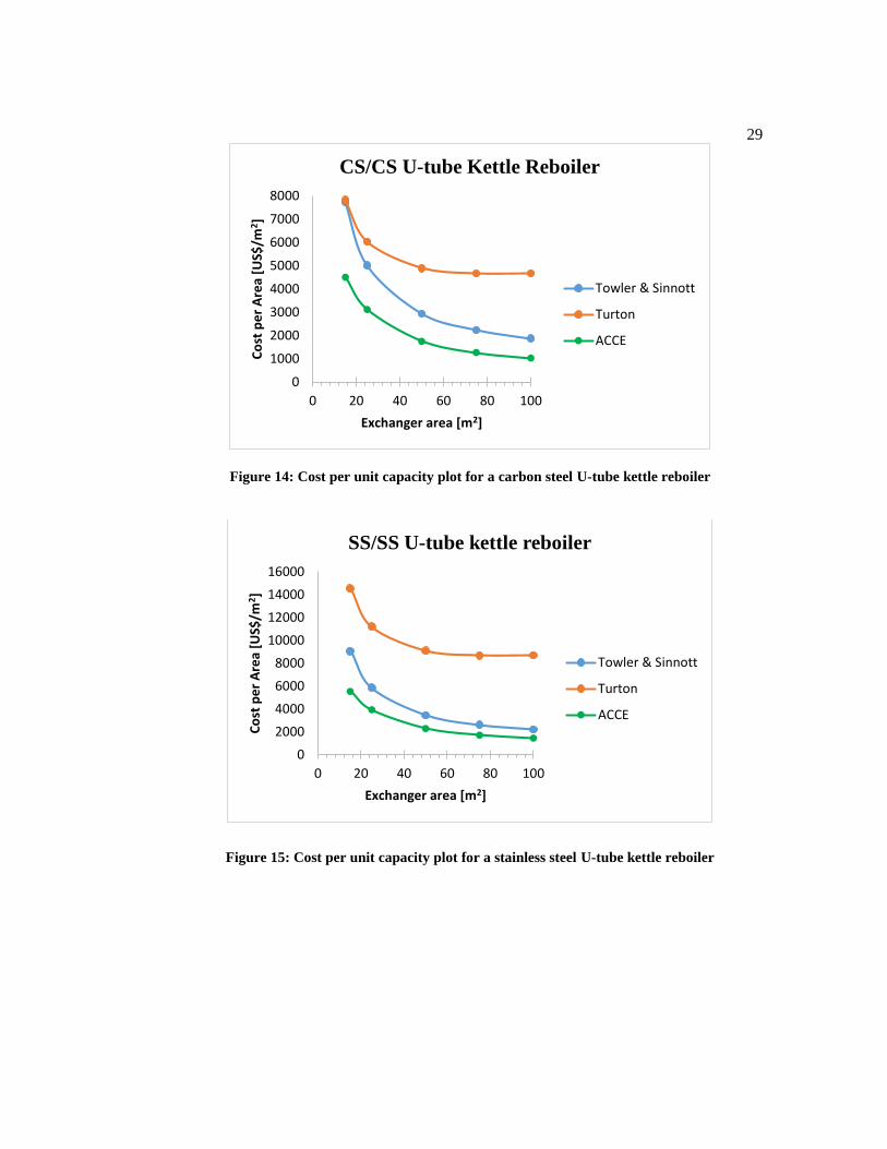
Kettle Reboiler
Figure 13 and Figure 14 show the cost per capacity plot on a dollar basis and a
dollar per square meter basis, respectively for carbon steel. Figure 15shows the
cost per capacity plot for the U-tube kettle reboiler on a dollar per square meter
basis for stainless steel. Turton’s method can be seen leveling out for both
materials.
Figure 13: Cost vs. capacity plot for a carbon steel U-tube kettle reboiler
4.8
5
5.2
5.4
5.6
5.8
1 1.5 2
Log
(Co
st in
US$
)
Log(Exchanger Area in m2)
CS/CS U-tube Kettle Reboiler
Towler &Sinnott
Turton
ACCE
29
Figure 14: Cost per unit capacity plot for a carbon steel U-tube kettle reboiler
Figure 15: Cost per unit capacity plot for a stainless steel U-tube kettle reboiler
0
1000
2000
3000
4000
5000
6000
7000
8000
0 20 40 60 80 100
Co
st p
er
Are
a [U
S$/m
2 ]
Exchanger area [m2]
CS/CS U-tube Kettle Reboiler
Towler & Sinnott
Turton
ACCE
0
2000
4000
6000
8000
10000
12000
14000
16000
0 20 40 60 80 100
Co
st p
er
Are
a [U
S$/m
2]
Exchanger area [m2]
SS/SS U-tube kettle reboiler
Towler & Sinnott
Turton
ACCE
30
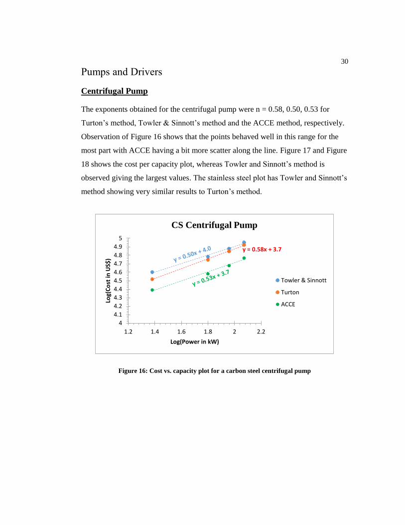
Pumps and Drivers
Centrifugal Pump
The exponents obtained for the centrifugal pump were n = 0.58, 0.50, 0.53 for
Turton’s method, Towler & Sinnott’s method and the ACCE method, respectively.
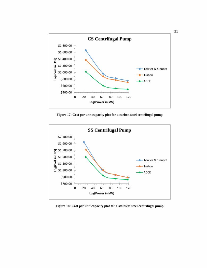
Observation of Figure 16 shows that the points behaved well in this range for the
most part with ACCE having a bit more scatter along the line. Figure 17 and Figure
18 shows the cost per capacity plot, whereas Towler and Sinnott’s method is
observed giving the largest values. The stainless steel plot has Towler and Sinnott’s
method showing very similar results to Turton’s method.
Figure 16: Cost vs. capacity plot for a carbon steel centrifugal pump
y = 0.58x + 3.7
4
4.1
4.2
4.3
4.4
4.5
4.6
4.7
4.8
4.9
5
1.2 1.4 1.6 1.8 2 2.2
Log(
Co
st in
US$
)
Log(Power in kW)
CS Centrifugal Pump
Towler & Sinnott
Turton
ACCE
31
Figure 17: Cost per unit capacity plot for a carbon steel centrifugal pump
Figure 18: Cost per unit capacity plot for a stainless steel centrifugal pump
$400.00
$600.00
$800.00
$1,000.00
$1,200.00
$1,400.00
$1,600.00
$1,800.00
0 20 40 60 80 100 120
Log(
Co
st in
US$
)
Log(Power in kW)
CS Centrifugal Pump
Towler & Sinnott
Turton
ACCE
$700.00
$900.00
$1,100.00
$1,300.00
$1,500.00
$1,700.00
$1,900.00
$2,100.00
0 20 40 60 80 100 120
Log(
Co
st in
US$
)
Log(Power in kW)
SS Centrifugal Pump
Towler & Sinnott
Turton
ACCE
32
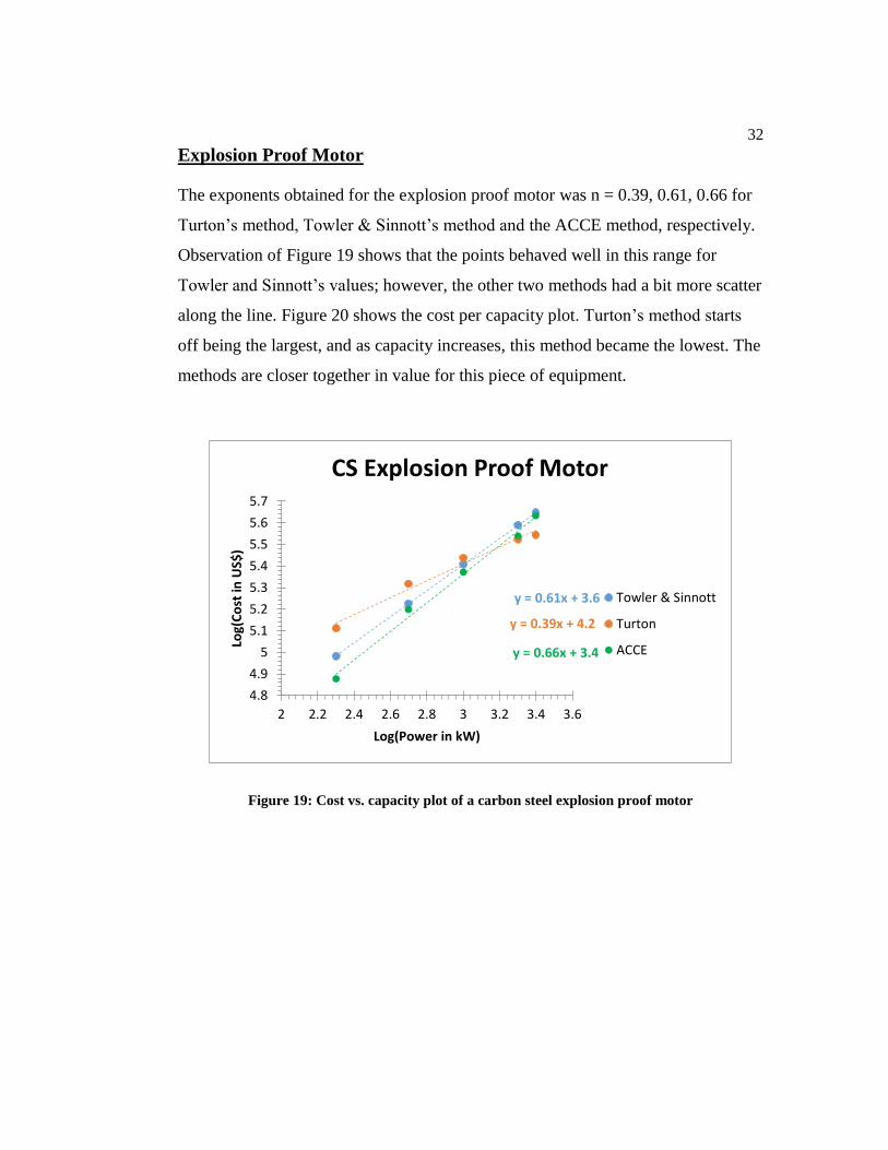
Explosion Proof Motor
The exponents obtained for the explosion proof motor was n = 0.39, 0.61, 0.66 for
Turton’s method, Towler & Sinnott’s method and the ACCE method, respectively.
Observation of Figure 19 shows that the points behaved well in this range for
Towler and Sinnott’s values; however, the other two methods had a bit more scatter
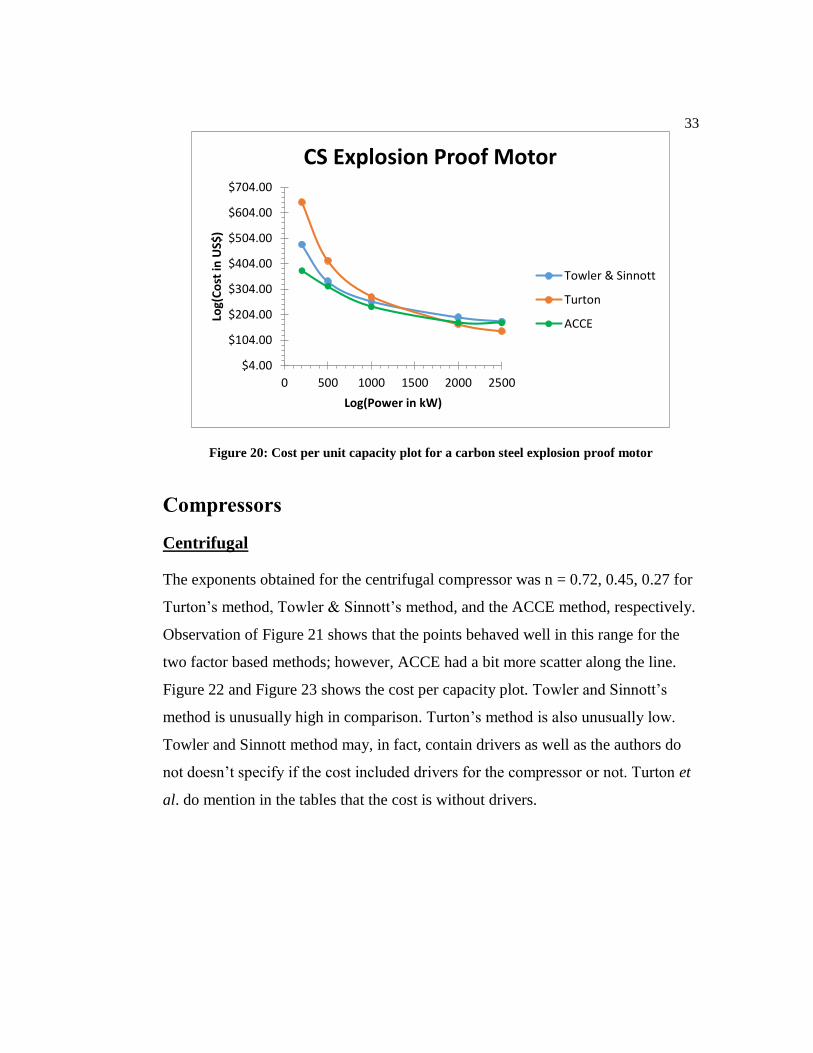
along the line. Figure 20 shows the cost per capacity plot. Turton’s method starts
off being the largest, and as capacity increases, this method became the lowest. The
methods are closer together in value for this piece of equipment.
Figure 19: Cost vs. capacity plot of a carbon steel explosion proof motor
y = 0.61x + 3.6
y = 0.39x + 4.2
y = 0.66x + 3.4
4.8
4.9
5
5.1
5.2
5.3
5.4
5.5
5.6
5.7
2 2.2 2.4 2.6 2.8 3 3.2 3.4 3.6
Log(
Co
st in
US$
)
Log(Power in kW)
CS Explosion Proof Motor
Towler & Sinnott
Turton
ACCE
33
Figure 20: Cost per unit capacity plot for a carbon steel explosion proof motor
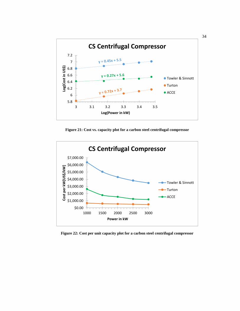
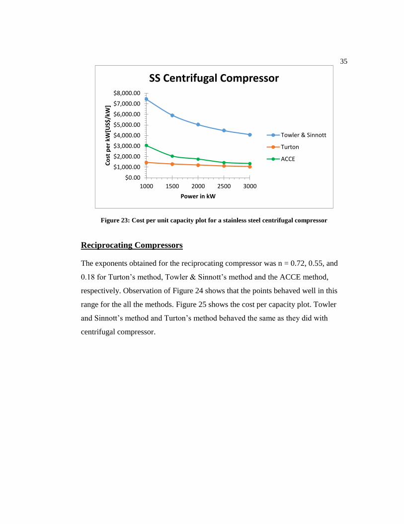
Compressors
Centrifugal
The exponents obtained for the centrifugal compressor was n = 0.72, 0.45, 0.27 for
Turton’s method, Towler & Sinnott’s method, and the ACCE method, respectively.
Observation of Figure 21 shows that the points behaved well in this range for the
two factor based methods; however, ACCE had a bit more scatter along the line.
Figure 22 and Figure 23 shows the cost per capacity plot. Towler and Sinnott’s
method is unusually high in comparison. Turton’s method is also unusually low.
Towler and Sinnott method may, in fact, contain drivers as well as the authors do
not doesn’t specify if the cost included drivers for the compressor or not. Turton et
al. do mention in the tables that the cost is without drivers.
$4.00
$104.00
$204.00
$304.00
$404.00
$504.00
$604.00
$704.00
0 500 1000 1500 2000 2500
Log(
Co
st in
US$
)
Log(Power in kW)
CS Explosion Proof Motor
Towler & Sinnott
Turton
ACCE
34
Figure 21: Cost vs. capacity plot for a carbon steel centrifugal compressor
Figure 22: Cost per unit capacity plot for a carbon steel centrifugal compressor
5.8
6
6.2
6.4
6.6
6.8
7
7.2
3 3.1 3.2 3.3 3.4 3.5
Log(
Co
st in
US$
)
Log(Power in kW)
CS Centrifugal Compressor
Towler & Sinnott
Turton
ACCE
$0.00
$1,000.00
$2,000.00
$3,000.00
$4,000.00
$5,000.00
$6,000.00
$7,000.00
1000 1500 2000 2500 3000
Co
st p
er
kW[U
S$/k
W]
Power in kW
CS Centrifugal Compressor
Towler & Sinnott
Turton
ACCE
35
Figure 23: Cost per unit capacity plot for a stainless steel centrifugal compressor
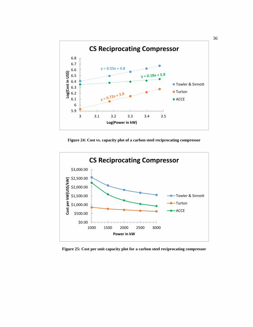
Reciprocating Compressors
The exponents obtained for the reciprocating compressor was n = 0.72, 0.55, and
0.18 for Turton’s method, Towler & Sinnott’s method and the ACCE method,
respectively. Observation of Figure 24 shows that the points behaved well in this
range for the all the methods. Figure 25 shows the cost per capacity plot. Towler
and Sinnott’s method and Turton’s method behaved the same as they did with
centrifugal compressor.
$0.00
$1,000.00
$2,000.00
$3,000.00
$4,000.00
$5,000.00
$6,000.00
$7,000.00
$8,000.00
1000 1500 2000 2500 3000
Co
st p
er
kW[U
S$/k
W]
Power in kW
SS Centrifugal Compressor
Towler & Sinnott
Turton
ACCE
36
Figure 24: Cost vs. capacity plot of a carbon steel reciprocating compressor
Figure 25: Cost per unit capacity plot for a carbon steel reciprocating compressor
y = 0.55x + 4.8
5.9
6
6.1
6.2
6.3
6.4
6.5
6.6
6.7
6.8
3 3.1 3.2 3.3 3.4 3.5
Log(
Co
st in
US$
)
Log(Power in kW)
CS Reciprocating Compressor
Towler & Sinnott
Turton
ACCE
$0.00
$500.00
$1,000.00
$1,500.00
$2,000.00
$2,500.00
$3,000.00
1000 1500 2000 2500 3000
Co
st p
er
kW[U
S$/k
W]
Power in kW
CS Reciprocating Compressor
Towler & Sinnott
Turton
ACCE
37
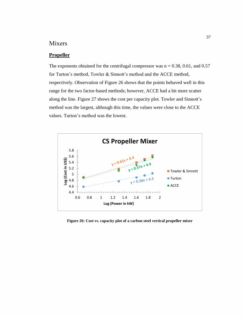
Mixers
Propeller
The exponents obtained for the centrifugal compressor was n = 0.38, 0.61, and 0.57
for Turton’s method, Towler & Sinnott’s method and the ACCE method,
respectively. Observation of Figure 26 shows that the points behaved well in this
range for the two factor-based methods; however, ACCE had a bit more scatter
along the line. Figure 27 shows the cost per capacity plot. Towler and Sinnott’s
method was the largest, although this time, the values were close to the ACCE
values. Turton’s method was the lowest.
Figure 26: Cost vs. capacity plot of a carbon steel vertical propeller mixer
4.4
4.6
4.8
5
5.2
5.4
5.6
5.8
0.6 0.8 1 1.2 1.4 1.6 1.8 2
Log
(Co
st in
US$
)
Log (Power in kW)
CS Propeller Mixer
Towler & Sinnott
Turton
ACCE

38
Figure 27: Cost per unit capacity plot for a carbon steel propeller mixer
Validation of Results
The Aspen Capital Cost Estimator is so detailed in its cost reports that using it as a
benchmark is the other methods is justified. ACCE provides a detailed breakdown
of each individual item that contributes to the cost of the piece of equipment. The
program is also able to account for more detailed specifications which,
consequently and intuitively, will make the estimate more precise than the factor-
based methods. A sample report is shown in Appendix C. It shows all the design
data used in the cost engine as well as a summary of all the installation costs and
estimated man hours needed and the cost for those man hours.
The six-tenths rule may be used as another tool for validation of the results as it is
based off of actual vendor data as well. According to Brown19, this is one of the
most useful relationships in cost engineering as it is valid for both equipment
purchase and plant and process costs. However, he also goes on to say that the
charts should be used with caution as the cost data for these charts were 20 to 45
years old19. This data is, of course, even older now. Brown19 also has a list of data
$0
$5,000
$10,000
$15,000
$20,000
0 20 40 60 80
Co
st p
er
kW [
US$
/kW
]
Power [kW]
CS Propeller Mixer
Towler & Sinnott
Turton
ACCE
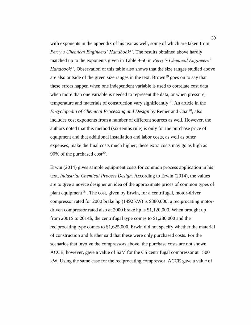
39
with exponents in the appendix of his text as well, some of which are taken from
Perry’s Chemical Engineers’ Handbook17. The results obtained above hardly
matched up to the exponents given in Table 9-50 in Perry’s Chemical Engineers’
Handbook17. Observation of this table also shows that the size ranges studied above
are also outside of the given size ranges in the text. Brown19 goes on to say that
these errors happen when one independent variable is used to correlate cost data
when more than one variable is needed to represent the data, or when pressure,
temperature and materials of construction vary significantly19. An article in the
Encyclopedia of Chemical Processing and Design by Remer and Chai20, also
includes cost exponents from a number of different sources as well. However, the
authors noted that this method (six-tenths rule) is only for the purchase price of
equipment and that additional installation and labor costs, as well as other
expenses, make the final costs much higher; these extra costs may go as high as
90% of the purchased cost20.
Erwin (2014) gives sample equipment costs for common process application in his
text, Industrial Chemical Process Design. According to Erwin (2014), the values
are to give a novice designer an idea of the approximate prices of common types of
plant equipment 21. The cost, given by Erwin, for a centrifugal, motor-driver
compressor rated for 2000 brake hp (1492 kW) is $880,000; a reciprocating motor-
driven compressor rated also at 2000 brake hp is $1,120,000. When brought up
from 2001$ to 2014$, the centrifugal type comes to $1,280,000 and the
reciprocating type comes to $1,625,000. Erwin did not specify whether the material
of construction and further said that these were only purchased costs. For the
scenarios that involve the compressors above, the purchase costs are not shown.
ACCE, however, gave a value of $2M for the CS centrifugal compressor at 1500
kW. Using the same case for the reciprocating compressor, ACCE gave a value of

40
$2M also, which is within the limits of error. This price, in ACCE, could be larger
or smaller based on the specified inlet and outlet flow rates.
41
Chapter 6
Conclusions and Recommendations
Error! Not a valid bookmark self-reference. summarizes the results obtained by
each method. Turton’s method had an average exponent of 0.63, while Towler &
Sinnott’s method and ACCE had average exponents of 0.55 and 0.41, respectively.
For most of the equipment, both Turton’s module costing method and Towler and
Sinnott’s factorial method, when compared to the ACCE, was within the -30 to
50% margin of error as laid out by the AACI for class 4 estimates4. The heat
exchangers, however, were on the high side with the factorial method showing
differences as high as 100% of the ACCE value for the floating head type; these
same differences are seen also for the kettle reboiler with the module costing
method. This trend was also seen in comparisons done by Feng in which the DFP
program’s costs (based on the factorial method) were also really high in
comparison12. Major differences in the results come down to the availability of
pricing data and the accuracy with which cost curves are made. As mentioned
before, Towler and Sinnott’s factorial method does not take into account the type of
equipment being costed. The result of this is every piece of equipment being
multiplied by the same factors, similar to the Lang factor method, with the addition
of the material factors. This method does not account for design pressures either.
Turton’s method, on the other hand, accounts for pressure and materials of
construction in most of its equipment. However, some equipment like mixers and
compressors do not account for changes in these factors.
42
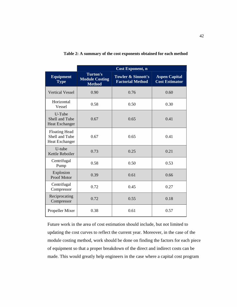
Table 2: A summary of the cost exponents obtained for each method
Cost Exponent, n
Equipment
Type
Turton's
Module Costing
Method
Towler & Sinnott's
Factorial Method
Aspen Capital
Cost Estimator
Vertical Vessel 0.90 0.76 0.60
Horizontal
Vessel 0.58 0.50 0.30
U-Tube
Shell and Tube
Heat Exchanger
0.67 0.65 0.41
Floating Head
Shell and Tube
Heat Exchanger
0.67 0.65 0.41
U-tube
Kettle Reboiler 0.73 0.25 0.21
Centrifugal
Pump 0.58 0.50 0.53
Explosion
Proof Motor 0.39 0.61 0.66
Centrifugal
Compressor 0.72 0.45 0.27
Reciprocating
Compressor 0.72 0.55 0.18
Propeller Mixer 0.38 0.61 0.57
Future work in the area of cost estimation should include, but not limited to
updating the cost curves to reflect the current year. Moreover, in the case of the
module costing method, work should be done on finding the factors for each piece
of equipment so that a proper breakdown of the direct and indirect costs can be
made. This would greatly help engineers in the case where a capital cost program
43
cannot be afforded. As mentioned before, the equipment chosen was based on the
support of all three methods; more equipment could be added even to get a
comparison of at least two methods. If possible, one could try to correlate only
purchased cost. Work could also be done to get factors out of Aspen by way of
reverse engineering the costs or by another method. Other methods, such as, Seider
and Seader’s11 module costing method could also be incorporated into the study.
44
References
1. D.W. Green RHP. Perry’s Chemical Engineer's Handbook. Eighth Edi. New
York: McGraw-Hill; 2008. doi:10.1036/0071422943.
2. Couper JR, Penney WR, Fair JR, Walas SM. Chemical Process Equipment -
Process and Design (3rd Edition). (Couper JR, Penney WR, Fair JR, Walas
SM, eds.). Elsevier; 2010. doi:10.1016/B978-0-12-372506-6.00009-5.
3. Turton R, Bailie R, Whiting W, Shaeiwitz JA, Bhattacharyya D. Analysis,
Synthesis, and Design of Chemical Processes. 4th Editio. Prentice Hall;
2013.
4. Christensen P, Dysert LR, Bates J, Burton D, Creese RC, Hollmann J. Cost
Estimate Classification system-as applied in engineering, procurement, and
construction for the process industries. 2005.
http://www.aacei.org/toc/toc_18R-97.pdf.
5. Towler G, Sinnot R. Chemical Engineering Design: Principles, Practice and
Economics of Plant and Process Design.; 2012.
6. Ereev S, Patel M. Recommended methodology and tool for cost estimates at
micro level for new technologies. Rep Prosuite 227078. 2011;(November
2009).
7. Farrar G. Estimated Nelson-Farrar quarterly costs: Annual indices for
refinery construction that have been posted for 80 years, from 1926 to the
present . Oil Gas J Latinoam. 2008;14(1):24-27.
http://www.scopus.com/inward/record.url?eid=2-s2.0-
52249117491&partnerID=40&md5=609911a07146e6fd756cc74f465c414f.
8. Peters MS, Timmerhaus KD. Plant Design and Economics for Chemical
Engineers. 4th ed. New York: McGraw-Hill, Inc; 1991.
9. Ashuri B, Lu J. Time Series Analysis of ENR Construction Cost Index. J
45
Constr Eng Manag. 2010;136(11):1227-1237.
10. Economic Indicators. Chem Eng. 2015;122(12):192.
www.chemengonline.com/pci.
11. Seider WD, Seader JD, Lewin DR. Product & Process Design Principles -
Synthesis, Analysis & Evaluation. Chemistry (Easton). 2003:728.
12. Feng Y, Rangaiah GP. Evaluating Capital Cost Estimation Programs. Chem
Eng. 2011;(8):22-29. http://www.chemengonline.com/evaluating-capital-
cost-estimation-programs-3/.
13. Aspen Technology Inc. Aspen Capital Cost Estimator: User’s Guide.
version 8. Burlington, MA; 2012. http://www.aspentech.com.
14. Beck R. Model-Based Conceptual Estimating. 2011.
https://www.brainshark.com/aspentech1/ACCE_vs_factored?em=whitlow@
fit.edu.
15. Beck R. Relative Costing During Conceptual Design with Aspen Plus. 2010.
https://www.brainshark.com/aspentech1/vu?pi=zH0zPx7dIz29bpz0.
16. Aspen Technology Inc. Aspen Capital Cost Estimator. 2015.
http://www.aspentech.com/products/economic-evaluation/aspen-capital-
cost-estimator/.
17. GREEN DW, PERRY RH. PERRY’S CHEMICAL ENGINEERS'
HANDBOOK. 7th editio. New York: McGraw-Hill; 1997.
18. MEPS International Ltd. MEPS - STEEL PRICES ONLINE.
http://www.meps.co.uk/index-price.htm. Published 2015. Accessed
December 23, 2015.
19. Brown T. Engineering Economics and Economic Design for Process
Engineers. CRC Press; 2006.
https://books.google.com/books?id=8dHHdQOT55IC&pgis=1.
20. Remer DS, Chai LH. Process Equipment , Cost Scale-up. In: Encyclopedia
of Chemical Processing and Design. ed. Marcel Dekker, Inc.; 1993:306-317.
21. Erwin DLPE. Process Equipment Cost Determination. In: Industrial
Chemical Process Design. Second. McGraw-Hill Professional; 2014:414.
46
Appendix A
Additional Equations used for Pressure Vessels
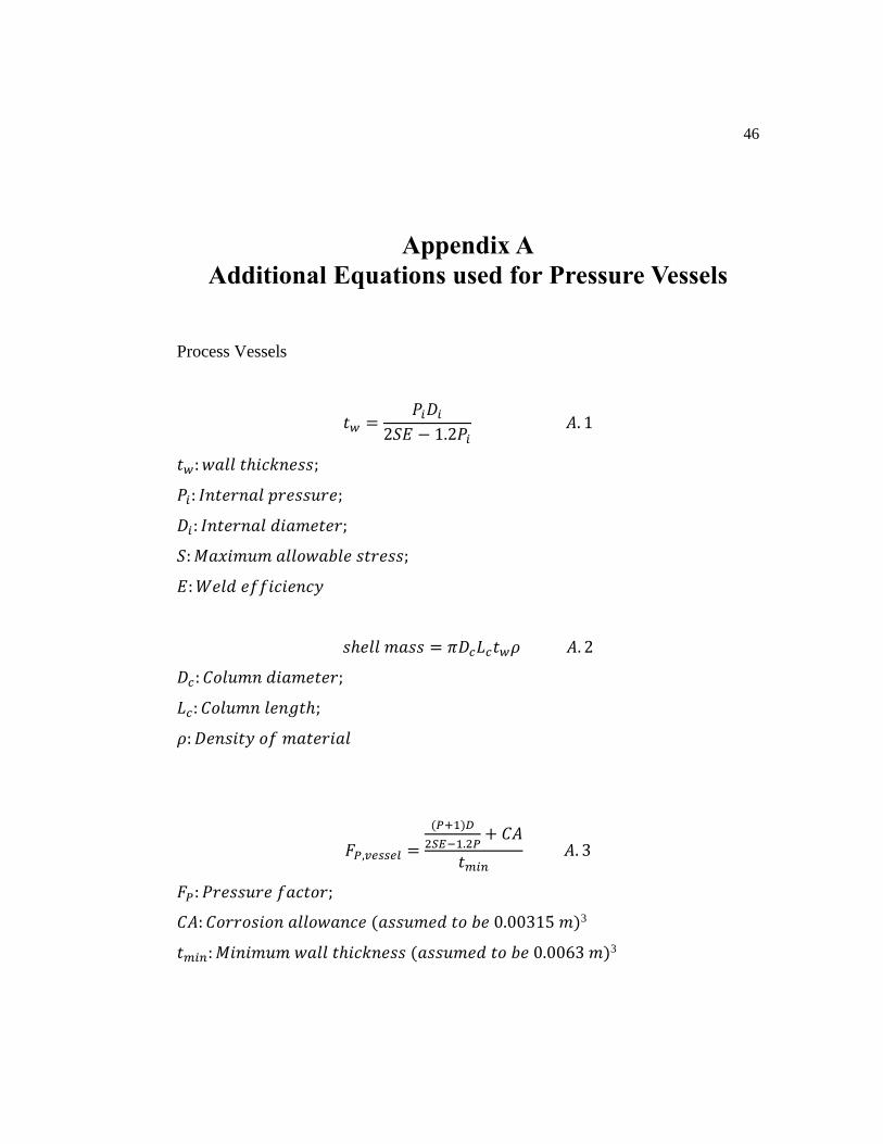
Process Vessels
𝑡𝑤 =𝑃𝑖𝐷𝑖
2𝑆𝐸 − 1.2𝑃𝑖 𝐴. 1
𝑡𝑤: 𝑤𝑎𝑙𝑙 𝑡ℎ𝑖𝑐𝑘𝑛𝑒𝑠𝑠;
𝑃𝑖: 𝐼𝑛𝑡𝑒𝑟𝑛𝑎𝑙 𝑝𝑟𝑒𝑠𝑠𝑢𝑟𝑒;
𝐷𝑖: 𝐼𝑛𝑡𝑒𝑟𝑛𝑎𝑙 𝑑𝑖𝑎𝑚𝑒𝑡𝑒𝑟;
𝑆: 𝑀𝑎𝑥𝑖𝑚𝑢𝑚 𝑎𝑙𝑙𝑜𝑤𝑎𝑏𝑙𝑒 𝑠𝑡𝑟𝑒𝑠𝑠;
𝐸: 𝑊𝑒𝑙𝑑 𝑒𝑓𝑓𝑖𝑐𝑖𝑒𝑛𝑐𝑦
𝑠ℎ𝑒𝑙𝑙 𝑚𝑎𝑠𝑠 = 𝜋𝐷𝑐𝐿𝑐𝑡𝑤𝜌 𝐴. 2
𝐷𝑐: 𝐶𝑜𝑙𝑢𝑚𝑛 𝑑𝑖𝑎𝑚𝑒𝑡𝑒𝑟;
𝐿𝑐: 𝐶𝑜𝑙𝑢𝑚𝑛 𝑙𝑒𝑛𝑔𝑡ℎ;
𝜌: 𝐷𝑒𝑛𝑠𝑖𝑡𝑦 𝑜𝑓 𝑚𝑎𝑡𝑒𝑟𝑖𝑎𝑙
𝐹𝑃,𝑣𝑒𝑠𝑠𝑒𝑙 =
(𝑃+1)𝐷
2𝑆𝐸−1.2𝑃+ 𝐶𝐴
𝑡𝑚𝑖𝑛 𝐴. 3
𝐹𝑃: 𝑃𝑟𝑒𝑠𝑠𝑢𝑟𝑒 𝑓𝑎𝑐𝑡𝑜𝑟;
𝐶𝐴: 𝐶𝑜𝑟𝑟𝑜𝑠𝑖𝑜𝑛 𝑎𝑙𝑙𝑜𝑤𝑎𝑛𝑐𝑒 (𝑎𝑠𝑠𝑢𝑚𝑒𝑑 𝑡𝑜 𝑏𝑒 0.00315 𝑚)3
𝑡𝑚𝑖𝑛: 𝑀𝑖𝑛𝑖𝑚𝑢𝑚 𝑤𝑎𝑙𝑙 𝑡ℎ𝑖𝑐𝑘𝑛𝑒𝑠𝑠 (𝑎𝑠𝑠𝑢𝑚𝑒𝑑 𝑡𝑜 𝑏𝑒 0.0063 𝑚)3
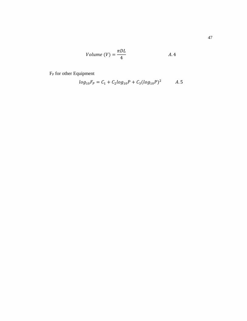
47
𝑉𝑜𝑙𝑢𝑚𝑒 (𝑉) =𝜋𝐷𝐿
4 𝐴. 4
FP for other Equipment
𝑙𝑜𝑔10𝐹𝑃 = 𝐶1 + 𝐶2𝑙𝑜𝑔10𝑃 + 𝐶3(𝑙𝑜𝑔10𝑃)2 𝐴. 5
48
Appendix B
The Aspen Capital Cost Estimator user interface
1. After opening the software, left-click on new project.
2. Enter a the name of your project in the window that pops up then click ‘ok’
3. You may choose whether to use metric or imperial units in the next window
that pops up then click ‘ok’
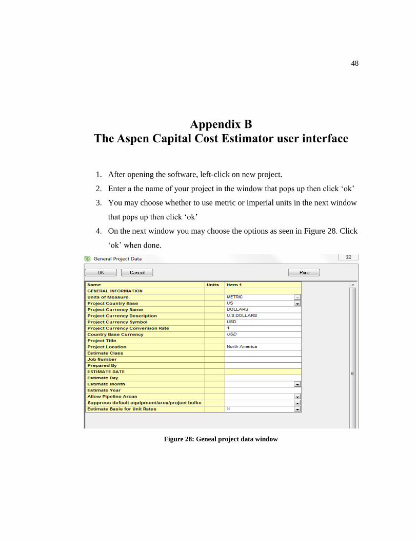
4. On the next window you may choose the options as seen in Figure 28. Click
‘ok’ when done.
Figure 28: Geneal project data window
49
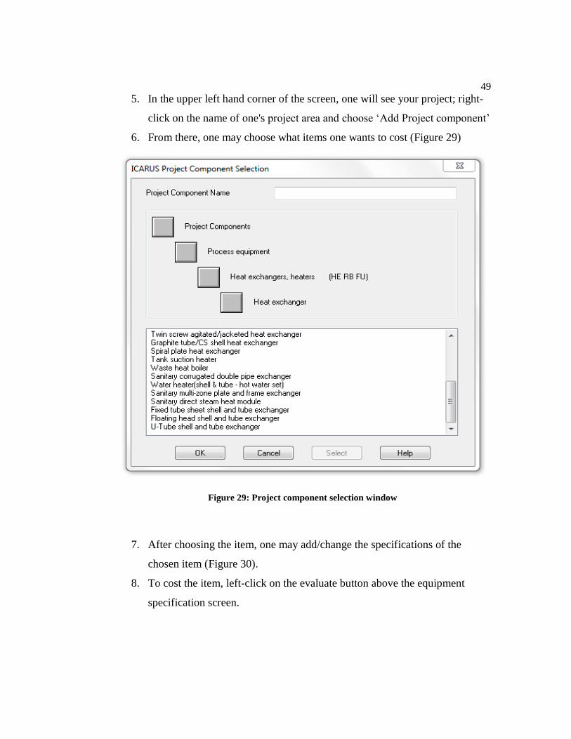
5. In the upper left hand corner of the screen, one will see your project; right-
click on the name of one's project area and choose ‘Add Project component’
6. From there, one may choose what items one wants to cost (Figure 29)
Figure 29: Project component selection window
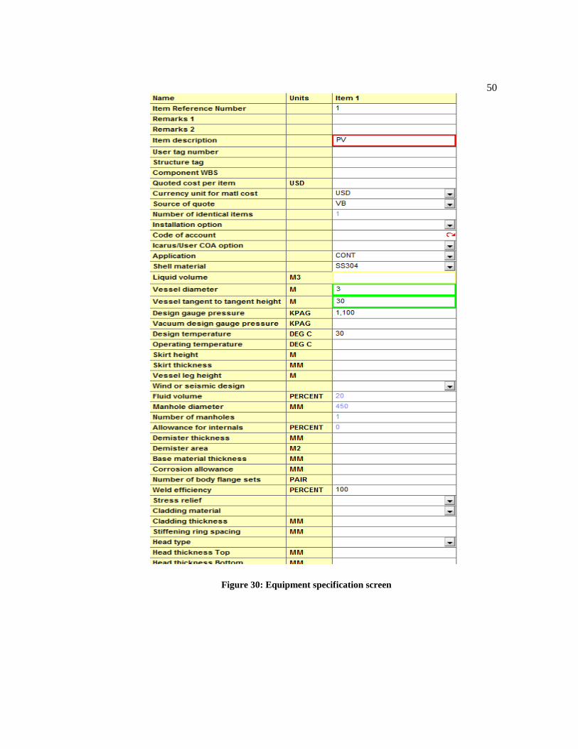
7. After choosing the item, one may add/change the specifications of the
chosen item (Figure 30).
8. To cost the item, left-click on the evaluate button above the equipment
specification screen.
50
Figure 30: Equipment specification screen
51
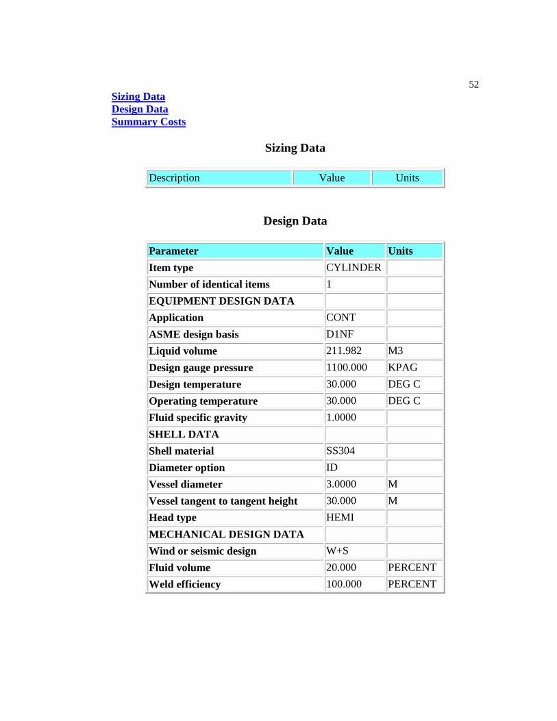
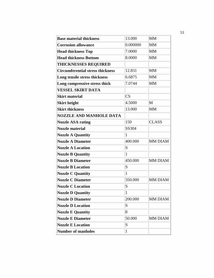
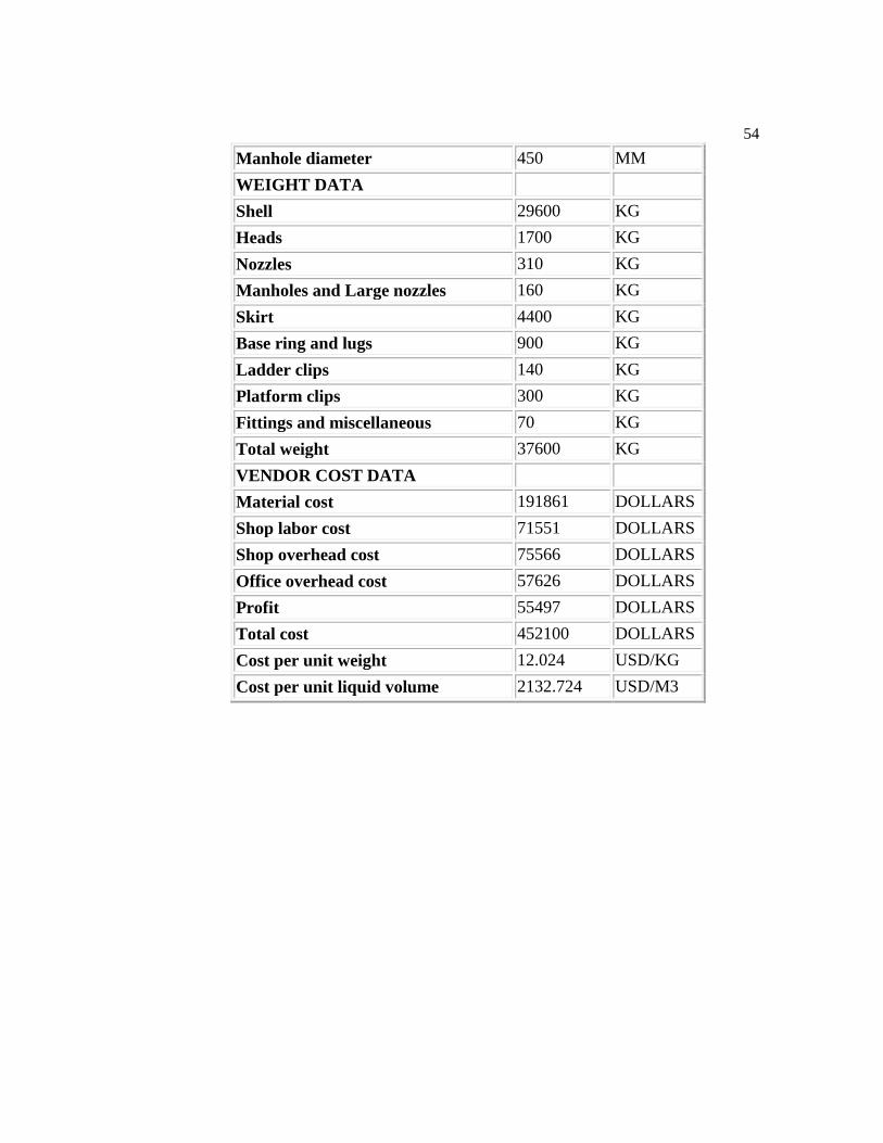
Appendix C
ACCE Sample Item Report
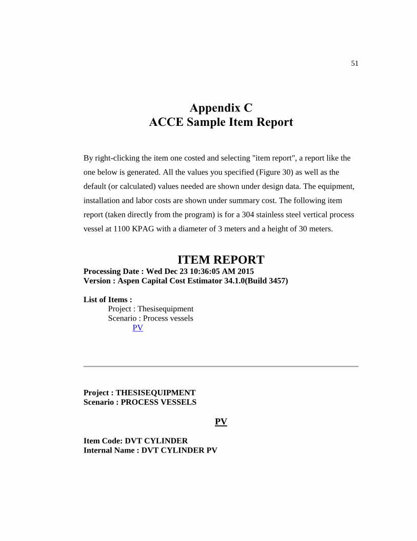
By right-clicking the item one costed and selecting "item report", a report like the
one below is generated. All the values you specified (Figure 30) as well as the
default (or calculated) values needed are shown under design data. The equipment,
installation and labor costs are shown under summary cost. The following item
report (taken directly from the program) is for a 304 stainless steel vertical process
vessel at 1100 KPAG with a diameter of 3 meters and a height of 30 meters.
ITEM REPORT Processing Date : Wed Dec 23 10:36:05 AM 2015
Version : Aspen Capital Cost Estimator 34.1.0(Build 3457)
List of Items : Project : Thesisequipment
Scenario : Process vessels
PV
Project : THESISEQUIPMENT
Scenario : PROCESS VESSELS
PV
Item Code: DVT CYLINDER
Internal Name : DVT CYLINDER PV
52
Sizing Data
Design Data
Summary Costs
Sizing Data
Description Value Units
Design Data
Parameter Value Units
Item type CYLINDER
Number of identical items 1
EQUIPMENT DESIGN DATA
Application CONT
ASME design basis D1NF
Liquid volume 211.982 M3
Design gauge pressure 1100.000 KPAG
Design temperature 30.000 DEG C
Operating temperature 30.000 DEG C
Fluid specific gravity 1.0000
SHELL DATA
Shell material SS304
Diameter option ID
Vessel diameter 3.0000 M
Vessel tangent to tangent height 30.000 M
Head type HEMI
MECHANICAL DESIGN DATA
Wind or seismic design W+S
Fluid volume 20.000 PERCENT
Weld efficiency 100.000 PERCENT
53
Base material thickness 13.000 MM
Corrosion allowance 0.000000 MM
Head thickness Top 7.0000 MM
Head thickness Bottom 8.0000 MM
THICKNESSES REQUIRED
Circumferential stress thickness 12.831 MM
Long tensile stress thickness 6.6875 MM
Long compressive stress thick 7.0744 MM
VESSEL SKIRT DATA
Skirt material CS
Skirt height 4.5000 M
Skirt thickness 13.000 MM
NOZZLE AND MANHOLE DATA
Nozzle ASA rating 150 CLASS
Nozzle material SS304
Nozzle A Quantity 1
Nozzle A Diameter 400.000 MM DIAM
Nozzle A Location S
Nozzle B Quantity 1
Nozzle B Diameter 450.000 MM DIAM
Nozzle B Location S
Nozzle C Quantity 1
Nozzle C Diameter 350.000 MM DIAM
Nozzle C Location S
Nozzle D Quantity 1
Nozzle D Diameter 200.000 MM DIAM
Nozzle D Location S
Nozzle E Quantity 8
Nozzle E Diameter 50.000 MM DIAM
Nozzle E Location S
Number of manholes 1
54
Manhole diameter 450 MM
WEIGHT DATA
Shell 29600 KG
Heads 1700 KG
Nozzles 310 KG
Manholes and Large nozzles 160 KG
Skirt 4400 KG
Base ring and lugs 900 KG
Ladder clips 140 KG
Platform clips 300 KG
Fittings and miscellaneous 70 KG
Total weight 37600 KG
VENDOR COST DATA
Material cost 191861 DOLLARS
Shop labor cost 71551 DOLLARS
Shop overhead cost 75566 DOLLARS
Office overhead cost 57626 DOLLARS
Profit 55497 DOLLARS
Total cost 452100 DOLLARS
Cost per unit weight 12.024 USD/KG
Cost per unit liquid volume 2132.724 USD/M3
55
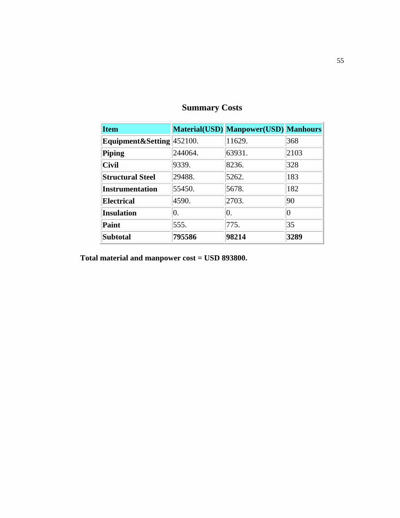
Summary Costs
Item Material(USD) Manpower(USD) Manhours
Equipment&Setting 452100. 11629. 368
Piping 244064. 63931. 2103
Civil 9339. 8236. 328
Structural Steel 29488. 5262. 183
Instrumentation 55450. 5678. 182
Electrical 4590. 2703. 90
Insulation 0. 0. 0
Paint 555. 775. 35
Subtotal 795586 98214 3289
Total material and manpower cost = USD 893800.