an analysis of cpc’s operational 0.5-month lead seasonal

An Analysis of CPC’s Operational 0.5-Month Lead Seasonal Outlooks

PEITAO PENG, ARUN KUMAR, AND MICHAEL S. HALPERT

NOAA/Climate Prediction Center, Washington, D.C.

ANTHONY G. BARNSTON

International Research Institute for Climate and Society, Earth Institute, Columbia University, Palisades, New York

(Manuscript received 22 November 2011, in final form 10 February 2012)

ABSTRACT

An analysis and verification of 15 years of Climate Prediction Center (CPC) operational seasonal surface

temperature and precipitation climate outlooks over the United States is presented for the shortest and most

commonly used lead time of 0.5 months. The analysis is intended to inform users of the characteristics and skill

of the outlooks, and inform the forecast producers of specific biases or weaknesses to help guide development

of improved forecast tools and procedures. The forecast assessments include both categorical and probabi-

listic verification diagnostics and their seasonalities, and encompass both temporal and spatial variations in

forecast skill. A reliability analysis assesses the correspondence between the forecast probabilities and their

corresponding observed relative frequencies. Attribution of skill to specific physical sources is discussed.

ENSO and long-term trends are shown to be the two dominant sources of seasonal forecast skill. Higher

average skill is found for temperature than for precipitation, largely because temperature benefits from trends

to a much greater extent than precipitation, whose skill is more exclusively ENSO based. Skill over the United

States is substantially dependent on season and location. The warming trend is shown to have been repro-

duced, but considerably underestimated, in the forecasts. Aside from this underestimation, and slight over-

confidence in precipitation forecast probabilities, a fairly good correspondence between forecast probabilities

and subsequent observed relative frequencies is found. This confirms that the usually weak forecast proba-

bility anomalies, while disappointing to some users, are justified by normally modest signal-to-noise ratios.

1. Introduction

Operational seasonal outlooks for surface mean tem-

perature and total precipitation over the United States

have been routinely made by the Climate Prediction

Center (CPC) since December 1994 and now span a 15-yr

period. The seasonal outlook information is disseminated

to the user community in several formats, for example,

the probabilities of tercile-based categories (Fig. 1) or

probability of exceedance (POE) (Barnston et al. 2000).

The CPC seasonal outlooks for surface temperature

and precipitation are released around the middle of the

calendar month; the first target season being the next

3-month period. For example, the first target season for

the seasonal outlook released in the middle of June is for

the climate conditions averaged over the July–September

(JAS) season. Beginning with the first target period, sea-

sonal outlooks are issued for the upcoming 13 overlapping

seasons, extending out to approximately 1 yr. This anal-

ysis and verification procedure is applied to the outlooks

for the first (0.5 month) lead time. It is intended to help

inform the user community about the past performance of

the operational seasonal outlooks, providing guidance on

the potential utility of the real-time forecast information

for decision making processes. The skill assessments are

also useful for the producers of the seasonal outlooks,

informing them of potential systematic biases in the

forecast tools in order that they may focus on improving

such weaknesses.

The analyses are aimed at defining the spatial and

temporal variations of performance, including seasonal

dependence, spanning the assessment of categorical and

probabilistic aspects of the forecasts (section 3). The

analyses also attempt to provide insight into the sources

Corresponding author address: Dr. Arun Kumar, 5200 Auth Rd.,

Camp Springs, MD 20746.

E-mail: [email protected]

898 W E A T H E R A N D F O R E C A S T I N G VOLUME 27

DOI: 10.1175/WAF-D-11-00143.1

� 2012 American Meteorological SocietyUnauthenticated | Downloaded 12/23/21 12:24 PM UTC

of skill (section 4). The present analyses extend recent

summaries of the CPC seasonal outlooks presented by

O’Lenic et al. (2008) and Livezey and Timofeyeva (2008).

In section 5 we discuss the use and interpretation of the

probabilistic seasonal climate outlook information, and

the potential utility for beneficial societal application of

the real-time seasonal forecasts within the context of the

verification findings.

2. Forecast format, data, verification methods,and sources of prediction skill

a. Seasonal outlook format

A comprehensive summary of seasonal prediction

methods used for generating the operational seasonal

outlooks at the CPC, and their historical evolution, appears

in O’Lenic et al. (2008); a brief overview is presented here.

CPC’s seasonal outlooks rely on a combination of

empirical and dynamical prediction tools (Van den Dool

2007; Trocolli et al. 2008). Empirical seasonal prediction

methods depend on identifying relationships between

a set of predictors (e.g., sea surface temperature) and the

forecast variables (i.e., surface temperature and pre-

cipitation), based on historical observed data (e.g., Barnston

1994). Dynamical seasonal prediction methods rely on

comprehensive general circulation models (GCMs) that are

initialized from the observed states for the different com-

ponents of the Earth system—ocean, land, atmosphere,

etc.—and are integrated forward in time (Ji et al. 1994).

Seasonal outlooks for U.S. surface temperature and

precipitation are probabilistic in nature, detailing shifts in

the probabilities, where they exist, away from their cli-

matological values (of 1/3) for three equiprobable tercile-

based categories. The category boundaries are defined

using observational data over the most recently com-

pleted 30-yr base period covering three decades (e.g.,

1981–2010 at the time of this writing). The categories

(often called simply terciles) are referred to as below,

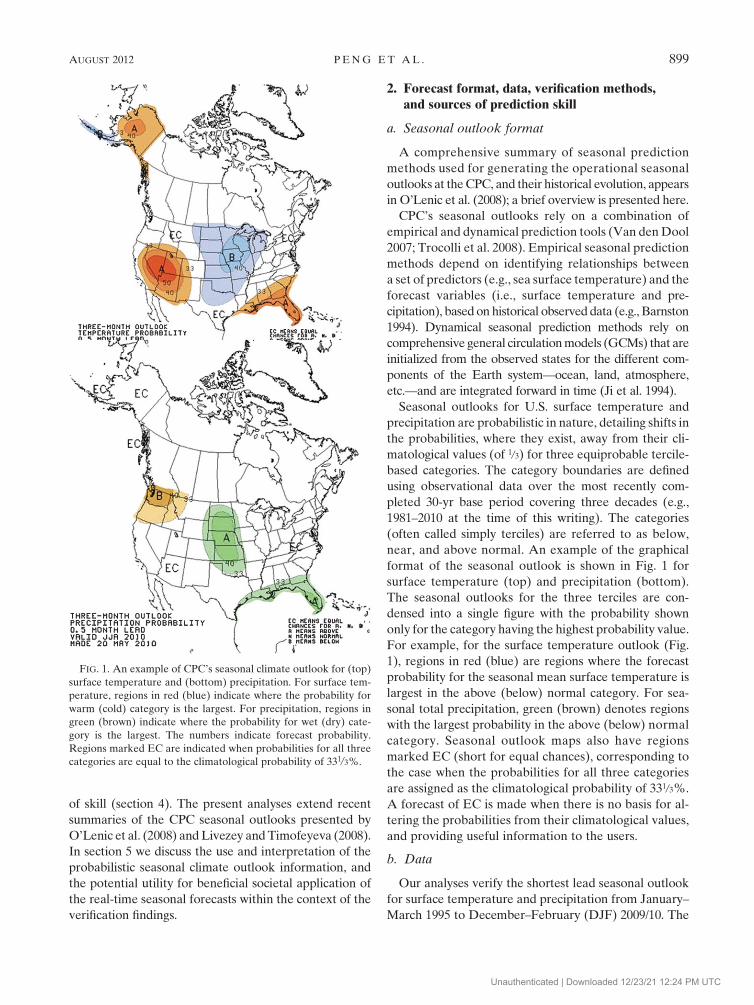
near, and above normal. An example of the graphical

format of the seasonal outlook is shown in Fig. 1 for

surface temperature (top) and precipitation (bottom).

The seasonal outlooks for the three terciles are con-

densed into a single figure with the probability shown

only for the category having the highest probability value.

For example, for the surface temperature outlook (Fig.

1), regions in red (blue) are regions where the forecast

probability for the seasonal mean surface temperature is

largest in the above (below) normal category. For sea-

sonal total precipitation, green (brown) denotes regions

with the largest probability in the above (below) normal

category. Seasonal outlook maps also have regions

marked EC (short for equal chances), corresponding to

the case when the probabilities for all three categories

are assigned as the climatological probability of 331/3%.

A forecast of EC is made when there is no basis for al-

tering the probabilities from their climatological values,

and providing useful information to the users.

b. Data

Our analyses verify the shortest lead seasonal outlook

for surface temperature and precipitation from January–

March 1995 to December–February (DJF) 2009/10. The

FIG. 1. An example of CPC’s seasonal climate outlook for (top)

surface temperature and (bottom) precipitation. For surface tem-

perature, regions in red (blue) indicate where the probability for

warm (cold) category is the largest. For precipitation, regions in

green (brown) indicate where the probability for wet (dry) cate-

gory is the largest. The numbers indicate forecast probability.

Regions marked EC are indicated when probabilities for all three

categories are equal to the climatological probability of 331/3%.

AUGUST 2012 P E N G E T A L . 899

Unauthenticated | Downloaded 12/23/21 12:24 PM UTC

spatial domain of the analysis is the continental United

States, despite the fact that CPC’s outlooks also in-

clude Hawaii and Alaska. Seasonal outlook probabilities,

and the verification data, are interpolated onto a 28 3 28

latitude–longitude spatial grid. Corresponding observa-

tions for surface temperature and precipitation come

from a CPC analysis. The tercile boundaries for seasonal

means for forecasts issued prior to May 2001 are based on

the observational data for the 1961–90 period, while for

forecasts issued from May 2001 and later the 1971–2000

period are used. The same change in the climatological

period is applied in computing the observed seasonal

mean anomalies for verification, and for determining the

category of the observed seasonal means.

c. Verification measures

Verification of the seasonal outlooks is done using

both categorical and probabilistic measures. For a cate-

gorical verification of the outlook, the Heidke skill score

(HSS; O’Lenic et al. 2008) is used. The HSS tallies the

number of ‘‘hits’’ (locations in which the category hav-

ing the highest forecast probability matches the later

observed category), and compares this number to the

number expected by chance in the absence of any skill.

The HSS is a scaled measure of the percentage im-

provement in skill relative to a climatology (EC) fore-

cast, and is defined as

HSS 5(c 2 e) 3 100

(t 2 e), (1)

where c is the number of grid points with hits, t is the

total number of grid points in the outlook, and e is

number of grid points expected to be correct by chance

(and equals t/3). In the case of more than one category

having the highest forecast probability, a hit is divided if

one of them is later observed. In CPC’s outlooks, two-

way ties never occur;1 in the case of the EC forecast

there is a three-way tie and thus one-third of a hit is

always tallied, equaling the hit rate expected by chance

and contributing to a zero HSS.

The HSS can be computed in two ways: 1) for all

points, including those where the EC forecast is issued,

and 2) for only points where the outlook differs from

EC. The latter is referred to as HSS1, while the former is

referred to as HSS2. By definition, jHSS1j$ jHSS2j and

both are scaled to range from 250 (when the forecast

categories at all of the points are incorrect) to 100 (when

the forecast categories at all points are correct). Maxi-

mizing HSS2 encourages making non-EC forecasts

wherever a forecast signal is believed to exist, even if

weak. On the other hand, HSS1 values may be maxi-

mized by making non-EC forecasts over only a small

region where the confidence in the forecast is highest. In

the extreme case, a non-EC forecast may be issued at

only the one point at which the forecasters are most

highly confident, and if that forecast results in a hit

(miss), the HSS1 score is 100% (250%).

As a measure of categorical skill, the HSS disregards

the magnitude of the outlook probabilities that indicate

the forecast confidence level, which is of importance

from the user’s decision making perspective. To verify

the probabilistic information in the seasonal outlooks,

the ranked probability skill score (RPSS) is used. The

RPSS is a measure of the squared distance between the

forecast and the observed cumulative probabilities;

a detailed discussion is found in Kumar et al. (2001) and

Wilks (2006). As a final assessment tool, we also use

reliability diagrams (Wilks 2006) to compare the fore-

cast probabilities against their corresponding frequen-

cies of observed occurrence to estimate systematic

biases in the assigned probabilities, the frequency dis-

tribution of the issued probabilities (i.e., sharpness), and

other characteristics of the forecasts.

Skill measures are computed either as time series, or

as spatial maps. For the time series analyses, the skill

score is computed between the seasonal outlook and the

verifying analysis averaged over the entire forecast

spatial domain.2 Alternatively, at each grid point, fore-

cast skill between the outlook and the verification time

series is computed as averaged over the entire period of

record, and the geographical distribution of local skill is

displayed as a map. These two approaches provide

complementary information. For example, while the

time series of skill illustrates how skill depends on the

temporal variation in the strength of predictors (e.g.,

interannual variations in the sea surface temperature in

the east-central tropical Pacific), the spatial map pro-

vides information about which regions have higher or

lower skill. Both dimensions of skill are expected to be

seasonally dependent.

d. A summary of forecast tools

The main predictors on which CPC’s seasonal outlooks

depend are the El Nino – Southern Oscillation (ENSO)

related SST variability, as well as low-frequency trends

1 Except for the case of the EC forecast, the near-normal cate-

gory is never given the same probability as the highest of the two

outer categories; furthermore, the two outer categories are never

tied in having the highest probability.

2 Because most of the grid points lie in a latitude band limited to

308–488N, latitude-dependent area weighting is not conducted.



(O’Lenic et al. 2008; Livezey and Timofeyeva 2008). In

making seasonal outlooks, the state of tropical Pacific

SSTs is first anticipated, using the corresponding tele-

connection signals over the United States when appro-

priate. The future state of the SSTs is generally based on

a combination of forecast guidance from empirical and

dynamical coupled model prediction tools (O’Lenic et al.

2008; Barnston et al. 2012). Another important tool used as

input to CPC’s seasonal climate outlooks is low-frequency

trends that are obtained based on the optimum climate

normal (OCN) methodology (Huang et al. 1996a). Fur-

ther discussion about the skill contributions of these tools

appears in section 4c.

Seasonal outlooks at the CPC also rely at times on

initial soil moisture anomalies and on guidance that in-

cludes land surface conditions provided by dynamical

prediction systems [e.g., the operational Climate Fore-

cast System (CFS) coupled model; Saha et al. (2006)].

Dynamical forecasts have the potential to contribute to

the skill of seasonal outlooks from the specification of

atmospheric, oceanic, and land initial conditions (akin to

that for medium-range weather prediction). However,

the relative contribution from the initial conditions is

difficult to quantify. Some analyses have shown that

even for short lead-time seasonal prediction, the in-

fluence of the longer-lasting boundary conditions dom-

inates (Kumar et al. 2011; Peng et al. 2011; Chen et al.

2010). In the preparation of the operational seasonal

outlooks, the trend and the ENSO-based signals, to-

gether with other tools, are merged together to form the

probability forecast.

3. Results

a. Coverage of seasonal outlooks

We first analyze the spatial and temporal variabilities

of the coverage of seasonal outlooks, with coverage

being defined as the percentage of grid points having

non-EC forecasts. The temporal analysis is done for

each season, consisting of a time series of the coverage.

Alternatively, the spatial analysis results in a map

showing the geographical distribution of the percent-

age of times the forecast at any location was non-EC.

Time series and spatial maps of coverage provide com-

plementary information. As expected for the forecast

skills, it is also expected that the temporal and spatial

variations in coverage should be attributable to known

physical mechanisms that contribute to predictability on

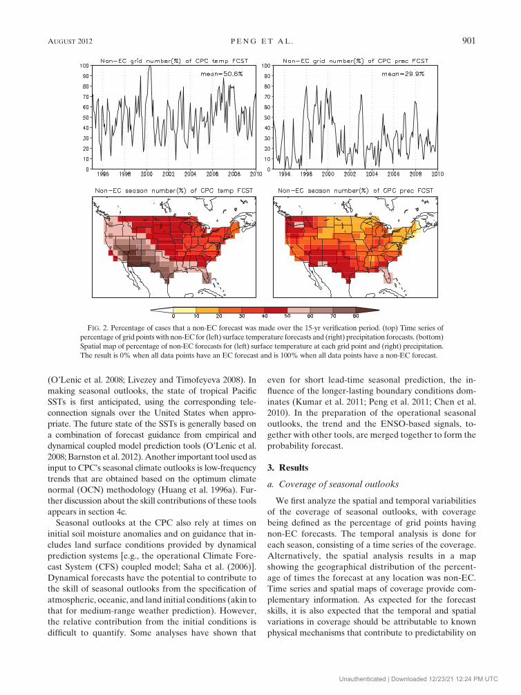
FIG. 2. Percentage of cases that a non-EC forecast was made over the 15-yr verification period. (top) Time series of

percentage of grid points with non-EC for (left) surface temperature forecasts and (right) precipitation forecasts. (bottom)

Spatial map of percentage of non-EC forecasts for (left) surface temperature at each grid point and (right) precipitation.

The result is 0% when all data points have an EC forecast and is 100% when all data points have a non-EC forecast.



seasonal time scales (e.g., ENSO) and exhibit seasonal

dependence.

Time series (Fig. 2, top) and spatial patterns (bottom)

show that the mean coverage for the temperature out-

looks was 50.6%, and for precipitation was 29.9%. If the

coverage of non-EC forecasts is an indication of pre-

dictability (or the signals) associated with the respective

variable, larger coverage for temperature is consistent

with the fact that it has more sources of predictability

than precipitation. Sources of predictability for tem-

perature include ENSO, trends, and initial soil mois-

ture anomalies. In contrast, most of the predictive skill

for precipitation comes from ENSO (Quan et al. 2006),

with signals from trend and soil moisture anomalies

smaller than for temperature (Huang et al. 1996a;

Huang et al. 1996b). Larger coverage for surface tem-

perature is also consistent with the substantially higher

skill of CPC’s forecasts for temperature than pre-

cipitation. Similar differences in the skill for tempera-

ture and precipitation have been reported in skill

analyses of operational forecasts or predictability based

on atmospheric GCM (AGCM) simulations (Barnston

et al. 2010; Fawcett et al. 2004; Goddard et al. 2003; Peng

et al. 2000).

Figure 2 (top) shows that the forecast coverage has

large variability among neighboring (and overlapping)

seasons, as well as more generally. The standard deviation

of coverage for both the temperature and precipitation

time series is approximately 20%. Large variability among

neighboring seasons seems at odds with the slow evolution

of the set of predictors upon which the seasonal outlooks

depend (e.g., ENSO, trends). This discrepancy may occur

because of the subjective nature of the seasonal outlooks

(including the rotation of the lead forecaster), incon-

sistencies among the various forecast tools (that rely on

different sources for prediction skill), and also the sea-

sonality in the spatial extent and strength of the signals

associated with the various predictors (particularly ENSO).

The time spectrum of the variability in the coverage is

better understood in terms of the autocorrelation for the

time series of skill (to be shown as a somewhat related

variable), to be discussed later.

The spatial pattern of the percentage coverage (Fig.

2, bottom left) for temperature has its largest values

over the southwestern United States and a minimum

over the northeast region. For precipitation (Fig. 2,

bottom right), the largest coverage is along the south-

ern tier of states and over the Northwest. These spatial

patterns can be attributed to the spatial structure of the

signals associated with known predictors. For preci-

pitation, non-EC seasonal outlooks are made much

more frequently in the southern and northwestern

United States, regions that correspond to well-known

signals related to ENSO (see Fig. 14 and Peng et al.

2000; Ropelewski and Halpert 1987). For temperature,

the maximum of non-EC seasonal outlooks over the

southwestern United States corresponds to the region

of positive surface temperature trends in recent de-

cades (Huang et al. 1996a).

The seasonalities of the percent of area forecast for

surface temperature and precipitation are shown in Fig. 3.

For precipitation (red curve), a clear pattern is shown,

FIG. 3. Seasonal cycle of percentage of non-EC forecasts over the 15-yr verification period for

(black curve) surface temperature and (red curve) precipitation. The seasonal cycle is from the

average, for each season, of the time series shown in the top row of Fig. 2.



with largest spatial coverage during winter and a mini-

mum in the summer. This is consistent with the seasonality

of ENSO-related precipitation signals over the United

States, and also with the seasonality of the tropical Pacific

ENSO SST anomaly amplitude that peaks during boreal

winter.

The seasonality of the coverage for surface temper-

ature forecasts has a more complicated structure with

the largest coverage during winter, a secondary peak

during summer (e.g., for June–August, JJA), and

minima during spring and especially fall. The winter

maximum is consistent with the larger amplitude of the

signal related to ENSO, and also with the larger trends

in temperature during boreal winter (examples to be

shown later in section 4c). Minima during the spring

and fall seasons are expected on the basis of the greater

difficulty, in the extratropics, in establishing persistent

climate anomaly signals during the transitional seasons

of climatological SST and the large-scale atmospheric

circulation patterns and, hence, more random, short-

lived anomaly patterns. A possible explanation for the

greater coverage in spring than fall is the use of soil

moisture conditions as one of the predictive tools in

spring, which may contribute to the peak in coverage in

subsequent summers as well.

b. Analysis of skill in the seasonal surfacetemperature outlook

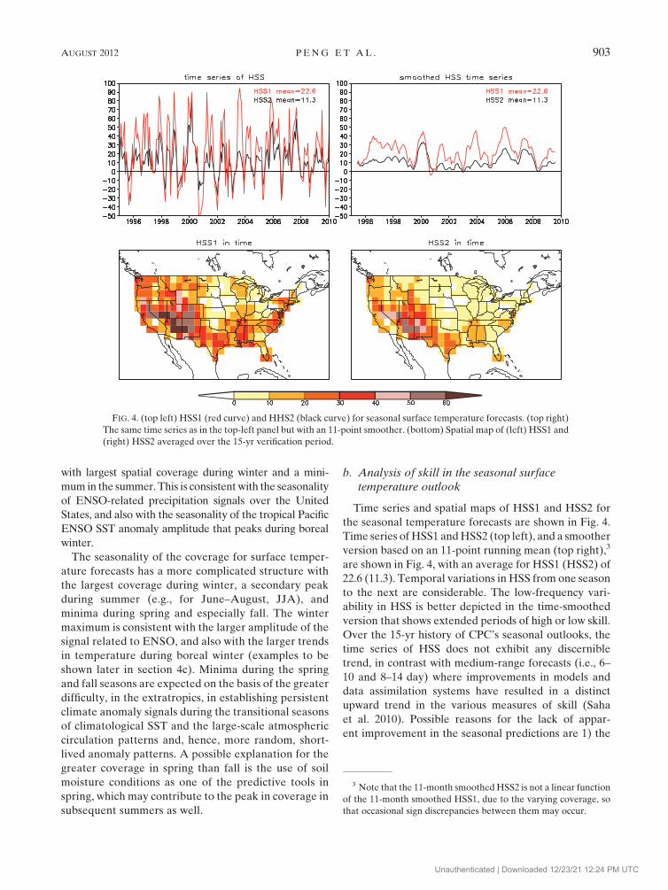
Time series and spatial maps of HSS1 and HSS2 for

the seasonal temperature forecasts are shown in Fig. 4.

Time series of HSS1 and HSS2 (top left), and a smoother

version based on an 11-point running mean (top right),3

are shown in Fig. 4, with an average for HSS1 (HSS2) of

22.6 (11.3). Temporal variations in HSS from one season

to the next are considerable. The low-frequency vari-

ability in HSS is better depicted in the time-smoothed

version that shows extended periods of high or low skill.

Over the 15-yr history of CPC’s seasonal outlooks, the

time series of HSS does not exhibit any discernible

trend, in contrast with medium-range forecasts (i.e., 6–

10 and 8–14 day) where improvements in models and

data assimilation systems have resulted in a distinct

upward trend in the various measures of skill (Saha

et al. 2010). Possible reasons for the lack of appar-

ent improvement in the seasonal predictions are 1) the

FIG. 4. (top left) HSS1 (red curve) and HHS2 (black curve) for seasonal surface temperature forecasts. (top right)

The same time series as in the top-left panel but with an 11-point smoother. (bottom) Spatial map of (left) HSS1 and

(right) HSS2 averaged over the 15-yr verification period.

3 Note that the 11-month smoothed HSS2 is not a linear function

of the 11-month smoothed HSS1, due to the varying coverage, so

that occasional sign discrepancies between them may occur.



generally lower level of skill, making a given modest

percentage improvement more difficult to discern amid

the large temporal fluctuations, and 2) the much smaller

number of temporal degrees of freedom on the seasonal

than medium-range weather time scale, such that the

chronology of high-amplitude climate events (e.g., ENSO

episodes, such as the one in the late 1990s) can more

strongly determine when skill is highest than can the

gradual improvement seen in the prediction models and

procedures.

The spatial distribution of HSS1 and HSS2 for tem-

perature over the 15 yr (Fig. 4, bottom) shows a prefer-

ence for higher skill in the southwestern United States

(with HSS1 approaching ;60–70), the northwest, and

across the southern tier of states. The lowest skill is found

in the central plains, part of the Ohio Valley and parts of

the northeast.

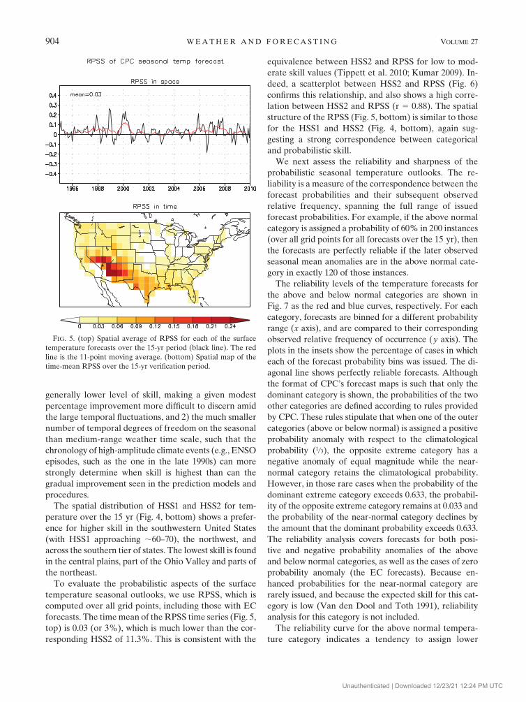
To evaluate the probabilistic aspects of the surface

temperature seasonal outlooks, we use RPSS, which is

computed over all grid points, including those with EC

forecasts. The time mean of the RPSS time series (Fig. 5,

top) is 0.03 (or 3%), which is much lower than the cor-

responding HSS2 of 11.3%. This is consistent with the

equivalence between HSS2 and RPSS for low to mod-

erate skill values (Tippett et al. 2010; Kumar 2009). In-

deed, a scatterplot between HSS2 and RPSS (Fig. 6)

confirms this relationship, and also shows a high corre-

lation between HSS2 and RPSS (r 5 0.88). The spatial

structure of the RPSS (Fig. 5, bottom) is similar to those

for the HSS1 and HSS2 (Fig. 4, bottom), again sug-

gesting a strong correspondence between categorical

and probabilistic skill.

We next assess the reliability and sharpness of the

probabilistic seasonal temperature outlooks. The re-

liability is a measure of the correspondence between the

forecast probabilities and their subsequent observed

relative frequency, spanning the full range of issued

forecast probabilities. For example, if the above normal

category is assigned a probability of 60% in 200 instances

(over all grid points for all forecasts over the 15 yr), then

the forecasts are perfectly reliable if the later observed

seasonal mean anomalies are in the above normal cate-

gory in exactly 120 of those instances.

The reliability levels of the temperature forecasts for

the above and below normal categories are shown in

Fig. 7 as the red and blue curves, respectively. For each

category, forecasts are binned for a different probability

range (x axis), and are compared to their corresponding

observed relative frequency of occurrence (y axis). The

plots in the insets show the percentage of cases in which

each of the forecast probability bins was issued. The di-

agonal line shows perfectly reliable forecasts. Although

the format of CPC’s forecast maps is such that only the

dominant category is shown, the probabilities of the two

other categories are defined according to rules provided

by CPC. These rules stipulate that when one of the outer

categories (above or below normal) is assigned a positive

probability anomaly with respect to the climatological

probability (1/3), the opposite extreme category has a

negative anomaly of equal magnitude while the near-

normal category retains the climatological probability.

However, in those rare cases when the probability of the

dominant extreme category exceeds 0.633, the probabil-

ity of the opposite extreme category remains at 0.033 and

the probability of the near-normal category declines by

the amount that the dominant probability exceeds 0.633.

The reliability analysis covers forecasts for both posi-

tive and negative probability anomalies of the above

and below normal categories, as well as the cases of zero

probability anomaly (the EC forecasts). Because en-

hanced probabilities for the near-normal category are

rarely issued, and because the expected skill for this cat-

egory is low (Van den Dool and Toth 1991), reliability

analysis for this category is not included.

The reliability curve for the above normal tempera-

ture category indicates a tendency to assign lower

FIG. 5. (top) Spatial average of RPSS for each of the surface

temperature forecasts over the 15-yr period (black line). The red

line is the 11-point moving average. (bottom) Spatial map of the

time-mean RPSS over the 15-yr verification period.



probabilities than are seen in the observed outcomes.

For example, the forecast probability for the above

normal category of 0.37 has been observed with a fre-

quency of ;0.5. This tendency is seen for nearly all of

the forecast probability bins, and it is clear that the

above normal category was generally probabilistically

underforecast. As one might expect, the opposite fore-

cast bias occurs for the below normal category, with the

observed relative frequencies much lower than the

forecast probabilities. Thus, the forecast probabilities

for temperature were generally biased toward under-

forecasting (overforecasting) the above (below) normal.

Despite the forecasters’ awareness of the tendency to-

ward above normal temperature observations in recent

decades, their mean forecast probabilities of 0.36 and

0.29 for above and below normal fall far short of the

observed relative frequencies of 0.47 and 0.23, re-

spectively. Such a cold bias, indicated by the general

vertical offset of the reliability curves with respect to the

458 perfect reliability line, was found in a study of the first

several years of the current period of CPC’s forecasts

(Wilks 2000), and also appeared in global probabilistic

temperature forecasts by International Research Insti-

tute for Climate Prediction (IRI; Barnston et al. 2010).

Despite the general cold forecast bias, the confidence

level of CPC’s temperature forecasts, indicated by the

slope of the reliability lines, appears reasonably good.

Lines with a slope steeper than 458 indicate under-

confidence, while lines with a slope shallower than 458

indicate overconfidence—a more frequently noted char-

acteristic of uncorrected dynamical model forecasts.

Overconfidence is characterized by greater differences in

forecast probability than the corresponding differences in

observed relative frequency.

The frequency distributions of the forecast probabil-

ities themselves (Fig. 7, inset diagrams) show, for both

the above and below normal categories, that the largest

frequency is for forecast probability denoting the EC

forecasts (0.333; shown as its own bar) and the two ad-

jacent probability bins (0.25–0.332 and 0.334–0.40), and

the frequency falls off rapidly for probability ranges

farther away from 0.33. Lower forecast frequencies at

the low or the high ends of the probability range are

indications of the conservative nature of the tempera-

ture outlooks, with ‘‘confident’’ forecast probabilities

seldom issued. This conservatism (low forecast sharp-

ness) may have consequences for decision making, where

actions are triggered based on probability thresholds

determined by a cost–loss analysis (Vizard et al. 2005;

Kumar 2010). For example, if a response is triggered at

a 60% forecast probability for the above normal tem-

perature category, then, given the forecast frequency

distribution (Fig. 7), an action will only be triggered on

very rare occasions.

The seasonality of the skill of surface temperature is

shown in Fig. 8. The HSS1 and HSS2 scores for each

season are averages of approximately 15 cases from 1995

to 2009 (Fig. 8, top). These scores are surprisingly con-

stant, with the summertime values similar to winter

scores. The largest HSS1 (red curve) value occurs during

JAS. However, due to the small sample, this relative peak

may not be significant, and is not seen as prominently in

FIG. 6. Scatterplot of RPSS (x axis) and HSS2 (y axis) for surface temperature over the 15-yr

verification period. The scatterplot is based on the unsmoothed time series of RPSS and HSS2

shown in Figs. 5 and 4, respectively.



HSS2. One would have expected skill for wintertime

temperature forecasts to be higher as ENSO tele-

connections over the United States are strongest then.

Further, as will be shown in section 4c, the trends as

depicted by the OCN are also largest for winter. On the

other hand, the atmospheric internal variability is also

the largest during winter, and it might counteract the

predictability implied in the larger signals associated

with ENSO and trend. The analysis in Kumar and

Hoerling (1998) demonstrated a similar seasonal cycle

of simulation skill based on atmospheric general circu-

lation model (AGCM) simulations forced with observed

SSTs. In the present study, the lowest skill level occurred

during the fall season. The seasonal cycles of HSS1 and

HSS2 are somewhat similar to the seasonality of the

percentage area of the forecast coverage (Fig. 3).

The spatial structures of HSS1 and HSS2 for the winter

and the summer seasons (Fig. 8) show a maximum in

prediction skill over the Southwest for both seasons. As

will be shown below in section 4c, the spatial pattern of

the summertime skill has a close resemblance to the

forecast guidance provided by the OCN tool. Further,

since the ENSO signal during summer will be shown to be

weak, most of the prediction skill is likely to be from the

trend-based OCN.

For the winter season, the combination of the pre-

dictive signal from the trend and ENSO creates a more

complex spatial structure of temperature prediction

skill. While the signal from the OCN prediction tool

generally favors above-normal temperatures over the

entire United States with the maximum over the northern

tier of states (see section 4c), where the interannual var-

iability of the seasonal mean is also the largest, the

El Nino (La Nina) signal is for warmer (colder) temper-

atures over the northern United States and colder

(warmer) conditions over the southern United States.

Therefore, depending on the amplitude and the phase of

ENSO, the associated signal could either be in or out of

phase with the OCN surface temperature signal. When

the two signals are of opposite (same) sign, a reduction

(enhancement) of predictive skill would occur, leading to

a spatial structure of skill that may not correspond to the

signal associated with either of the individual predictors.

Therefore, although the surface temperature signal is

FIG. 7. Reliability diagram for the above normal (red curve) and below normal (blue curve)

categories for all seasons and all grid points of surface temperature forecasts over the 15-yr

verification period. Least squares regression lines are shown, weighted by the sample sizes

represented by each point. The y 5 x diagonal line represents perfect reliability. The proba-

bilities are binned as 0.05-wide intervals, e.g., 0.20–0.25 (plotted at 0.225), except that the EC

forecasts (0.333) occupy their own bin and the lower and upper adjacent bins span 0.25–0.332

and 0.334–0.40, respectively. The inset histograms are the frequency distributions for these

probability bins for the (top left) above and (bottom right) below normal categories.



strongest over the northern United States, particularly

during winter, prediction skill there is not the highest; this

lack of correspondence may occur because of difficulties

in merging the forecast information based on ENSO with

that based on the trend, through the OCN.

c. Analysis of skill in the seasonal precipitationoutlook

The smoothed time series of HSS1 and HSS2 (top),

and the spatial pattern of HSS1 and HSS2 (middle and

bottom) for precipitation are shown in Fig. 9. Averaged

over the 15-yr period, the HSS1 (HSS2) score is 11.0

(2.5), which is smaller than the corresponding surface

temperature scores, demonstrating the difficulties asso-

ciated with the skillful prediction of seasonal total pre-

cipitation. Similar to surface temperature, the time

series over the 15-yr period does not show a discernible

upward trend. In fact, the longest stretch of high skill

appears early in the record from ;1996 to 1999, un-

doubtedly reflecting a heightened predictability associ-

ated with the 1997/98 El Nino episode followed by

a strong, prolonged La Nina event.

Shown in Fig. 10 is the seasonality of the time series of

spatially averaged HSS1 and HSS2 precipitation skill

levels (top), and the spatial structures of the HSS1 and

HSS2 skill levels in winter and summer. For HSS2 (black

FIG. 8. (top) Seasonal cycle of HSS1 (red curve) and HSS2 (black curve) for surface temperature forecasts over the

15-yr verification period. Seasonal cycle is the average, for each season, of the corresponding unsmoothed time series

in Fig. 4. Spatial distributions of the (middle left) HSS1 and (middle right) HSS2 skill levels for surface temperature

forecasts for DJF and (bottom row) JJA.



curve) the average skill tends to be highest during boreal

winter and early spring, and near zero during the re-

mainder of the year. This seasonality is consistent with

that of the ENSO-related precipitation signal. The sea-

sonality of HSS1 is noisier, with jumps in average skill

from one season to the next. This is likely an artifact of

the low skill values and the fact that the area covered by

the non-EC precipitation outlook is generally small but

highly variable (Fig. 2, top right). Hence, estimates of

HSS1 forecast skill tend to have large sampling errors

(Kumar 2009). A seasonal comparison of the spatial

structure of prediction skill supports the discussion

above, with higher skill during DJF than JJA. Therefore,

the spatial structure of skill for DJF (Fig. 10) is similar to

that for the annual mean (Fig. 9), and is reminiscent of

the winter precipitation signal related to ENSO (to be

discussed in greater detail in section 4c). This spatial

structure features higher skill in a band extending from

the Northwest across the central Rockies, and southern

tier of states to Florida, and along the East Coast. Al-

though there is a distinct dry (wet) signal related to El Nino

(La Nina) over the Ohio Valley, and a corresponding local

maximum in the frequency of non-EC forecasts there (Fig.

2, bottom right), the seasonal precipitation outlooks in that

region have not been skillful.

The reliability of the precipitation outlooks for the

above and below normal categories is shown in Fig. 11.

For forecast probabilities in the most frequently issued

probability bins between 0.25 and 0.40, the precipitation

outlook has fair reliability for both above and below

normal categories. However, above normal has been

slightly underforecast while below normal has been

slightly overforecast. The observed frequencies of ob-

servations have been greater for above normal (0.39)

than below normal (0.30), but the mean forecast prob-

abilities did not recognize this climate drift toward wet

and were 0.33 for both categories. The dry forecast bias

is small in comparison with the cold forecast bias noted

above for temperature.

The slopes of the reliability curves for both categories

indicate some degree of overconfidence. Because prob-

abilities of .40% and ,25% were forecast infrequently,

the reliability curves for those forecast probability bins

are subject to higher sampling variability (and are weighted

lightly in the regression lines). However, most of these

more extreme forecast probability bins show the dry

bias, and to a larger degree.

4. Further analysis of prediction skill

a. Relationship between frequency of issuance ofa non-EC forecast and predictive skill

Is there a relationship between the area covered by

non-EC forecasts and the skill of that individual fore-

cast? Similarly, is there a relationship between the fre-

quency with which a non-EC outlook is made at a grid

point and the corresponding time-mean skill at that grid

point? Intuitively, one would expect both to be true,

since the shift in forecast probabilities from climatology

is presumably warranted by signals associated with one

or more predictors (e.g., ENSO and/or trend). It is also

known that there is a positive relationship between the

signal strength (which would often result also in a greater

spatial extent) and the expected value of the forecast skill

(Kumar 2009). These two facts together argue for a link

between the frequency for the issuance of a non-EC

forecast and skill. To confirm these relationships for

FIG. 9. (top) HSS1 (red curve) and HSS2 (black curve) for sea-

sonal precipitation forecasts, after application of the 11-point

smoother of the original seasonal scores. Spatial map of time av-

erage of (middle) HSS1 and (bottom) HSS2 over the 15-yr verifi-

cation period.



CPC’s outlooks, we conduct the analysis in time by an-

alyzing the relationship between the coverage of non-

EC forecasts and average forecast skill of the given

forecast map, and in space by analyzing the geographical

distribution of the percentage of time a non-EC forecast

was made at a grid point against the time-average skill at

that point.

Shown in Fig. 12 are scatterplots for temperature

(top) and precipitation (bottom) for the spatial (left)

and temporal (right) analyses. In the temporal analysis,

the ENSO status of the forecast target season is in-

dicated by the colors (see caption). For the temperature

outlook, the frequency with which non-EC outlooks are

made at different locations does have a somewhat linear

relationship with the HSS1, with correlation 0.60 (Fig.

12, top left). Presumably, knowledge of signal(s) related

to some predictor(s) results in higher time-average skill.

This relationship, however, is not perfect, as there are

locations where the frequency of non-EC forecasts is

high (.70%), but average skill is near zero. For pre-

cipitation (Fig. 12, bottom left), a weaker, somewhat

linear, relationship is also observed.

On the other hand, the same analysis in the time do-

main (Fig. 12, right panels) shows no indication of a

linear relationship between the coverage of non-EC fore-

casts and skill, for both temperature and precipitation.

Larger coverage is shown during active ENSO periods,

particularly for precipitation, but higher HSS1 is not

clearly indicated for those cases. A possible explanation

for this result is that the HSS1 score carries no skill penalty

for small coverage of non-EC forecasts, and during times

of little or no signal the forecasters may be adept in

FIG. 10. As in Fig. 8, but for the seasonal precipitation forecasts.



deciding when a map should consist of mostly EC

forecasts, and at which grid points a very few non-EC

forecasts should be assigned. Thus, there may be just as

much opportunity for a high HSS1 for maps with a small

area of non-EC as maps with abundant non-EC areas.

One might expect, however, that in the latter case there

would be higher confidence in the interior portions of

the large signal areas, and that the presence of such

higher probability shifts might result in higher skill

levels. However, as shown in the reliability diagrams

(Figs. 7 and 11), most of the non-EC forecasts are issued

with probabilities differing only by 0.05–0.10 from 0.333,

especially for precipitation forecasts. This implies that

many of the large signal areas do not contain much

higher confidence in their interiors, but rather similar

probability anomalies to those closer to the periphery of

those areas. Moreover, a policy at CPC is that non-EC

forecast areas are never drawn unless the probability of

the dominant category equals or exceeds 0.40, which

ensures that even small areas contain one or more in-

terior location of adequate confidence.

When HSS2 is used for the time domain analyses,

a weak linear relationship between coverage and skill

appears (not shown), with correlations of 0.23 for tem-

perature and 0.21 for precipitation. While slightly more

toward expectation than the zero correlations seen for

HSS1, the weakness of the result begs explanation.

A possible explanation for the asymmetric behavior

for the spatial versus temporal analyses is as follows. For

the HSS time series, a high level of skill for an individual

season requires that the observed categories be the same

as the forecast categories over a sufficient fraction of the

area over which the prediction was made. Given that

seasonal mean variability comprises several different

modes of variability (Barnston and Livezey 1987), some

of which (e.g., the North Atlantic Oscillation) are not

predictable (Quan et al. 2006), a spatial coherence be-

tween the observed and forecast categories may be dif-

ficult to achieve, and may be highly variable over time.

On the other hand, it may be easier to obtain a sufficient

frequency of a match between the forecast and the ob-

served category at a fixed spatial location over a long

period of record. For example, if at a particular location

the basis for a high rate of issuance of a non-EC forecast

is due to the trend signal, the observed category may also

have a consistently higher likelihood to be the same as

the forecast.

b. Time variation in skill

In this section we examine the consistency of forecast

performance from one season to the next. This analysis

is interesting since the forecasts are likely to depend on

slowly evolving signals (e.g., trend or ENSO), but we

have seen that there is a rapid variation in observed skill

FIG. 11. As in Fig. 7 (reliability analysis), but for the precipitation forecasts. Above normal

precipitation is shown in green, and below normal in orange.



(Fig. 4). The autocorrelation for the HSS2 skill for sur-

face temperature and precipitation (Fig. 13) is computed

from the unsmoothed time series of HSS2 shown in the

top panels of Figs. 4 and 9, respectively. For a 1-month

lag, the autocorrelation for temperature (precipitation)

is only ;0.58 (;0.52), despite that adjacent seasonal

forecasts have two months in common. The autocorre-

lations fall to less than 0.1 for a 3-month lag, when there

is no overlap of months in the seasonal average. (Au-

tocorrelations for HSS1 are slightly lower than those for

HSS2: 1.00, 0.53, 0.24, and 0.01 for temperature, and

1.00, 0.31, 0.13, and 0.01 for precipitation.) The auto-

correlation expected for random time series, due purely

to the structural overlap of 1 or 2 months, is 0.67 for

seasons having 2 months in common and 0.33 for seasons

having 1 month in common. For HSS2, the autocorre-

lations for the overlapping seasons are lower than these

baselines. This may be due to the fact that since skill

depends both on forecasts as well as observations, the

autocorrelation in the time series of skill is affected by

the interplay of autocorrelation in those respective

time series (i.e., time series of forecasts and observed

seasonal means). Therefore, the autocorrelation of

a single random time series is likely not an appropriate

baseline.

c. An attribution analysis of skill

Seasonal prediction skill is generally attributed to

physical causes such as the local or remote influence of

slowly varying boundary conditions (e.g., SST or soil

moisture) and to the influence of low-frequency trends

relative to the climatology to which seasonal outlooks

are made (Kumar et al. 2007; Trenberth et al. 1998). The

state of the various predictors for seasonal outlooks

during the analysis period is next summarized—first for

temperature and then for precipitation.

FIG. 12. (top row) Scatterplot of percentage of non-EC forecasts (abscissa) and the corresponding HSS1 skill (or-

dinate) for surface temperature. (top left) The non-EC percentage and HSS1 skill for surface temperature in space

(corresponding to Fig. 2, bottom left, and Fig. 4, bottom left, respectively). (top right) The non-EC percentage and HSS1

skill for surface temperature in time (corresponding to Fig. 2, top left, and red line in Fig. 4, top left, respectively), with

the blue, black, and red dots denoting times of occurrence of La Nina, neutral, and El Nino conditions, respectively.

(bottom row) As in the top row, but for precipitation: (bottom left) non-EC percentage and HSS1 skill for precipitation

in space (corresponding to Fig. 2, bottom right, and Fig. 9, middle, respectively). (bottom right) The non-EC percentage

and HSS1 skill for precipitation in time [corresponding to Fig. 2, top right, and Fig. 9, top (red lines), respectively].



The U.S. surface temperature (Fig. 14, top) and pre-

cipitation (middle) patterns related to the warm phase of

ENSO are shown for winter (left) and summer (right).

(Details about the compositing procedure are described

online: http://www.cpc.noaa.gov/products/precip/CWlink/

ENSO/composites.) It is important to note that (a) there

is a considerable variability in the spatial structure of the

ENSO signal from summer to winter and (b) signals

have both positive and negative anomalies. Although

not shown, the signal for the cold phase of the ENSO

tends to be opposite of that for El Nino (Hoerling et al.

1997). The time series of the Nino-3.4 (58N–58S,

1708–1208W) SST anomaly [typically used to monitor

ENSO; Barnston et al. (1997)] is shown in the bottom-

most panel of Fig. 14. ENSO variability is marked by one

of the largest El Nino episodes (1997/98) followed by an

extended La Nina until early 2001. The period since

2001 has featured relatively short-lived El Nino and La

Nina episodes.

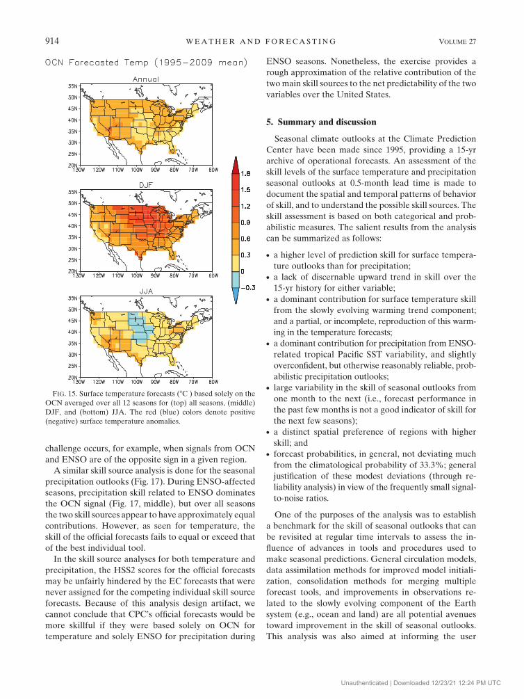
Seasonal forecast guidance for trends, based on the

OCN, is shown in Fig. 15. Averaged over the entire

analysis period and all seasons, the OCN has a warming

signal over the entire United States. However, seasonal

variability exists. For DJF (Fig. 15, middle), the entire

United States also has a warming trend signal, while for

summer (bottom) there is a cooling trend over the

central plains that has been referred to as the summer

warming hole (Wang et al. 2009). As the OCN meth-

odology depends on the difference in surface temper-

ature (precipitation) averaged over the last 10 (15) yr

relative to the 30-yr mean climatology for a given

season, the OCN forecasts vary only gradually from

one year to the next. This is in contrast to the ENSO-

related signal that depends on the phase and amplitude

of SST anomalies, which have considerable interannual

variability (Fig. 14).

In the final analysis we attempt to relate skill to its

possible sources discussed above, and estimate the sea-

sonal prediction skill for the trend and the ENSO signal

as individual forecast tools. For the trend we specify the

OCN alone as the seasonal outlook for each season, as is

used in the operational forecasts. For the ENSO-based

seasonal outlook, we first construct a regression pattern

for the respective variable related to the Nino-3.4 SST

using historical data, and then construct the outlook

using the regression pattern and the Nino-3.4 SST for

the target season.4 In constructing both the OCN- and

ENSO-based categorical forecasts, the forecast category

for each season is assigned based on the amplitude of the

forecast anomaly, and whichever category the forced

anomaly falls into based on the historical distribution

of the respective forecasts, and regions with EC do not

exist. (In the official CPC outlooks, the near-normal

category is used, but only occasionally.) HSS2 skill

scores for the individual tools are then compared with

the HSS2 for the CPC outlooks.

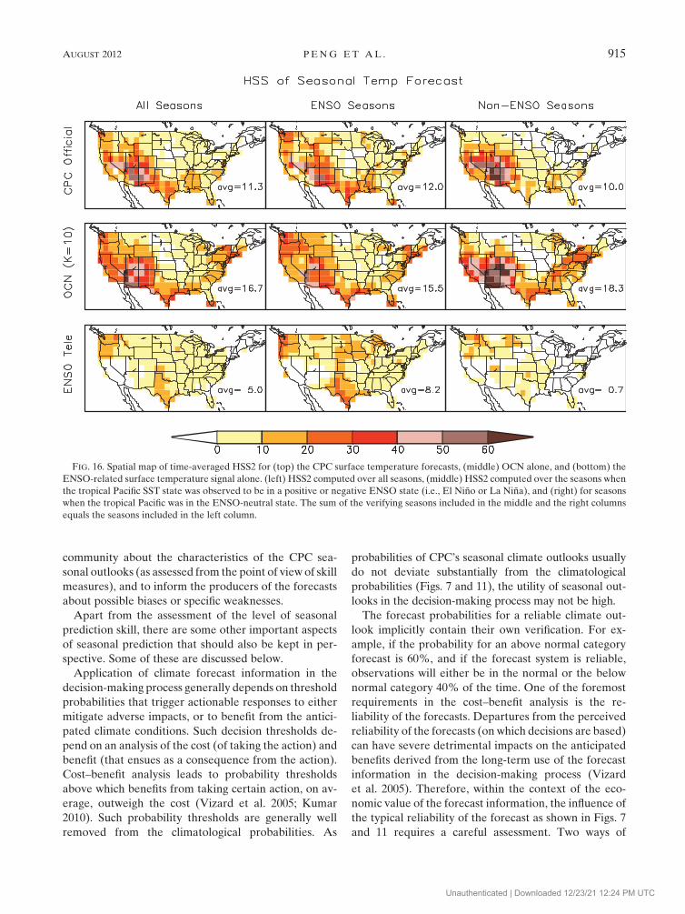
In Fig. 16 (left), the spatial distribution of HSS2 for

the official temperature forecast (top) is compared with

the HSS2 for OCN alone as the seasonal forecast

(middle) and for the ENSO-related temperature signal

(bottom), for all seasons. It is apparent that the HSS2 for

the official outlook has a very good resemblance with

the seasonal outlook based on the OCN. Further, the

spatial average of HSS2 for the OCN-based outlooks

(16.7) is better than the HSS2 from the ENSO-based

forecasts (5.0), as well as that from the official outlooks

(11.3). The analysis indicates that the dominant source

for the seasonal surface temperature outlook skill av-

eraged over all seasons is the trend-related information.

The lack of a strong contribution of the ENSO signal to

CPC’s temperature forecasts is consistent with findings

in Goddard et al. (2003) for the global temperature

forecasts issued by the IRI over a shorter period.

A likely cause of the lower HSS2 for the ENSO-based

surface temperature forecast is that ENSO is an episodic

phenomenon (see Fig. 14, bottom), and skillful forecasts

related to ENSO are possible when ENSO-related SST

anomalies are occurring. Furthermore, even during

ENSO episodes, climate impacts over the United States

are weak during the warm half of the year. On the other

hand, OCN, by definition, evolves more slowly, and

there is always a forecast signal associated with it that

affects some parts of the United States—during all years

FIG. 13. Autocorrelation of HSS2 skill time series as a function of

lag time (months) for surface temperature (blue bar) and pre-

cipitation (red bar) forecasts.

4 Here, we ignore the fact that we may occasionally, but in-

frequently, incorrectly predict the phase of ENSO for the target

period in an actual short-lead forecast and, therefore, expect that

the ENSO skill results may be slightly overestimated.



and all seasons. To test this hypothesis, we compute the

skill analysis for the ENSO and non-ENSO seasons. The

seasons with ENSO are defined using the categorization

developed at CPC (Kousky and Higgins 2007), as listed

online (http://www.cpc.ncep.noaa.gov/products/analysis_

monitoring/ensostuff/ensoyears.shtml).

A comparison of HSS2 for ENSO and non-ENSO

years is shown by the columns in Fig. 16. The HSS2 for

ENSO years (middle column) indicates that even for

ENSO seasons, the skill of the OCN exceeds that for

the ENSO-based forecasts, and is closer to the skill of

the CPC official outlooks. Similar results are also seen

in non-ENSO years, except that the HSS2 results for

ENSO-based forecasts are close to zero.

The fact that the OCN alone is found to have higher

HSS2 skill than that of the official outlook indicates

difficulties in merging the forecast information from

multiple predictors acting on different time scales. A

FIG. 14. (top left) DJF and (top right) JJA surface temperature composites for the warm phase of the ENSO (i.e.,

El Nino). (middle left) DJF and (middle right) JJA precipitation composites for warm phase of ENSO. (bottom) The

Nino-3.4 SST index over the analysis period.



challenge occurs, for example, when signals from OCN

and ENSO are of the opposite sign in a given region.

A similar skill source analysis is done for the seasonal

precipitation outlooks (Fig. 17). During ENSO-affected

seasons, precipitation skill related to ENSO dominates

the OCN signal (Fig. 17, middle), but over all seasons

the two skill sources appear to have approximately equal

contributions. However, as seen for temperature, the

skill of the official forecasts fails to equal or exceed that

of the best individual tool.

In the skill source analyses for both temperature and

precipitation, the HSS2 scores for the official forecasts

may be unfairly hindered by the EC forecasts that were

never assigned for the competing individual skill source

forecasts. Because of this analysis design artifact, we

cannot conclude that CPC’s official forecasts would be

more skillful if they were based solely on OCN for

temperature and solely ENSO for precipitation during

ENSO seasons. Nonetheless, the exercise provides a

rough approximation of the relative contribution of the

two main skill sources to the net predictability of the two

variables over the United States.

5. Summary and discussion

Seasonal climate outlooks at the Climate Prediction

Center have been made since 1995, providing a 15-yr

archive of operational forecasts. An assessment of the

skill levels of the surface temperature and precipitation

seasonal outlooks at 0.5-month lead time is made to

document the spatial and temporal patterns of behavior

of skill, and to understand the possible skill sources. The

skill assessment is based on both categorical and prob-

abilistic measures. The salient results from the analysis

can be summarized as follows:

d a higher level of prediction skill for surface tempera-

ture outlooks than for precipitation;d a lack of discernable upward trend in skill over the

15-yr history for either variable;d a dominant contribution for surface temperature skill

from the slowly evolving warming trend component;

and a partial, or incomplete, reproduction of this warm-

ing in the temperature forecasts;d a dominant contribution for precipitation from ENSO-

related tropical Pacific SST variability, and slightly

overconfident, but otherwise reasonably reliable, prob-

abilistic precipitation outlooks;d large variability in the skill of seasonal outlooks from

one month to the next (i.e., forecast performance in

the past few months is not a good indicator of skill for

the next few seasons);d a distinct spatial preference of regions with higher

skill; andd forecast probabilities, in general, not deviating much

from the climatological probability of 33.3%; general

justification of these modest deviations (through re-

liability analysis) in view of the frequently small signal-

to-noise ratios.

One of the purposes of the analysis was to establish

a benchmark for the skill of seasonal outlooks that can

be revisited at regular time intervals to assess the in-

fluence of advances in tools and procedures used to

make seasonal predictions. General circulation models,

data assimilation methods for improved model initiali-

zation, consolidation methods for merging multiple

forecast tools, and improvements in observations re-

lated to the slowly evolving component of the Earth

system (e.g., ocean and land) are all potential avenues

toward improvement in the skill of seasonal outlooks.

This analysis was also aimed at informing the user

FIG. 15. Surface temperature forecasts (8C ) based solely on the

OCN averaged over all 12 seasons for (top) all seasons, (middle)

DJF, and (bottom) JJA. The red (blue) colors denote positive

(negative) surface temperature anomalies.



community about the characteristics of the CPC sea-

sonal outlooks (as assessed from the point of view of skill

measures), and to inform the producers of the forecasts

about possible biases or specific weaknesses.

Apart from the assessment of the level of seasonal

prediction skill, there are some other important aspects

of seasonal prediction that should also be kept in per-

spective. Some of these are discussed below.

Application of climate forecast information in the

decision-making process generally depends on threshold

probabilities that trigger actionable responses to either

mitigate adverse impacts, or to benefit from the antici-

pated climate conditions. Such decision thresholds de-

pend on an analysis of the cost (of taking the action) and

benefit (that ensues as a consequence from the action).

Cost–benefit analysis leads to probability thresholds

above which benefits from taking certain action, on av-

erage, outweigh the cost (Vizard et al. 2005; Kumar

2010). Such probability thresholds are generally well

removed from the climatological probabilities. As

probabilities of CPC’s seasonal climate outlooks usually

do not deviate substantially from the climatological

probabilities (Figs. 7 and 11), the utility of seasonal out-

looks in the decision-making process may not be high.

The forecast probabilities for a reliable climate out-

look implicitly contain their own verification. For ex-

ample, if the probability for an above normal category

forecast is 60%, and if the forecast system is reliable,

observations will either be in the normal or the below

normal category 40% of the time. One of the foremost

requirements in the cost–benefit analysis is the re-

liability of the forecasts. Departures from the perceived

reliability of the forecasts (on which decisions are based)

can have severe detrimental impacts on the anticipated

benefits derived from the long-term use of the forecast

information in the decision-making process (Vizard

et al. 2005). Therefore, within the context of the eco-

nomic value of the forecast information, the influence of

the typical reliability of the forecast as shown in Figs. 7

and 11 requires a careful assessment. Two ways of

FIG. 16. Spatial map of time-averaged HSS2 for (top) the CPC surface temperature forecasts, (middle) OCN alone, and (bottom) the

ENSO-related surface temperature signal alone. (left) HSS2 computed over all seasons, (middle) HSS2 computed over the seasons when

the tropical Pacific SST state was observed to be in a positive or negative ENSO state (i.e., El Nino or La Nina), and (right) for seasons

when the tropical Pacific was in the ENSO-neutral state. The sum of the verifying seasons included in the middle and the right columns

equals the seasons included in the left column.



assessing the reliability of a forecast system are 1) to

build up a long history of the real-time seasonal outlooks

(as analyzed in this paper) and 2) to develop a set of

retrospective forecasts (i.e., hindcasts) that mimic as

closely as possible the real-time forecast setting. However,

continued upgrades to the forecast tools, particularly the

dynamical prediction systems, and the subjectivity in-

herent in CPC’s official forecast, make the second possi-

bility impractical.

From the perspective of the user of real-time climate

outlooks, the use of the skill information based on the

historical forecasts may still not be a straightforward

issue, with several factors posing challenging problems.

Skill information is an assessment of forecasts over

a long history that combines climate outlooks made

during many different climate conditions—for example,

the presence or absence of an ENSO event. Individual

real-time outlooks for a particular season and year, on

the other hand, are context dependent, and given the

climate conditions (e.g., the ENSO status) have their

own levels of skill. Stratification into such broad con-

ditional categories, which has been attempted here

for ENSO, can be informative, but carries sample size

reductions that increase sampling uncertainty. If prob-

abilistic forecasts have reasonably good reliability, the

anticipated level of skill is implicitly reflected in the

forecast probabilities. Thus, during high signal condi-

tions (e.g., a strong El Nino), skill levels can be antici-

pated to be higher than their average level for the given

season at some locations, with probabilities deviating

from 33% by greater amounts. How two sets of in-

formation (i.e., historical skill and skill implicit in the

forecast probabilities5) are to be used in the decision-

making context requires careful attention.

The analysis clearly points to the importance of recent

warming trends to the prediction skill for surface tem-

perature anomalies. With warming trends projected to

continue (Solomon et al. 2007), it is expected that trends

will remain an important source of temperature pre-

diction skill on seasonal time scales. It is important to

FIG. 17. As in Fig. 16 (HSS2 for official vs individual tool, for all forecasts and for forecasts stratified by ENSO status),

but for precipitation.

5 We should point out that these two sets of skill information are

sometimes referred to as conditional (skill score specific to a cli-

mate condition) and unconditional (skill score aggregated over the

full spectrum of climate conditions) skill scores (Kumar 2007).



recognize, however, that because the seasonal climate

outlooks are currently made relative to the mean of

a prior 30-yr period ending at the completion of the most

recent regular decade, the contribution of trends on pre-

diction skill may remain near the level documented here.

Acknowledgments. Comments by Dr. Dave Unger

and an anonymous reviewer helped improve the final

version of the manuscript.

REFERENCES

Barnston, A. G., 1994: Linear statistical short-term climate predictive

skill in the Northern Hemisphere. J. Climate, 7, 1514–1564.

——, and R. E. Livezey, 1987: Classification, seasonality and per-

sistence of low-frequency atmospheric circulation patterns.

Mon. Wea. Rev., 115, 1083–1126.

——, M. Chelliah, and S. B. Goldenberg, 1997: Documentation of

a highly ENSO-related SST region in the equatorial Pacific.

Atmos.–Ocean, 35, 367–383.

——, Y. He, and D. A. Unger, 2000: A forecast product that

maximizes utility for state-of-the-art seasonal climate pre-

dictions. Bull. Amer. Meteor. Soc., 81, 1271–1279.

——, L. Shuhua, S. J. Mason, D. G. DeWitt, L. Goddard, and

X. Gong, 2010: Verification of the first 11 years of IRI’s sea-

sonal climate forecasts. J. Appl. Meteor. Climatol., 49, 493–520.

——, M. K. Tippett, M. L. L’Heureux, S. Li, and D. G. DeWitt,

2012: Skill of real-time seasonal ENSO model predictions

during 2002–11—Is our capability increasing? Bull. Amer.

Meteor. Soc., 93, 631–651.

Chen, M., W. Wang, and A. Kumar, 2010: Prediction of monthly

mean temperature: The roles of atmospheric and land initial

condition and sea surface temperature. J. Climate, 23, 717–725.

Fawcett, R. J. B., D. A. Jones, and G. S. Beard, 2004: A verification

of publicly-issued seasonal forecasts issued by the Australian

government Bureau of Meteorology: 1998–2003. Aust. Meteor.

Mag., 54, 1–13.

Goddard, L., A. G. Barnston, and S. J. Mason, 2003: Evaluation of

the IRI’s ‘‘net assessment’’ seasonal climate forecasts. Bull.

Amer. Meteor. Soc., 84, 1761–1781.

Hoerling, M. P., A. Kumar, and M. Zhong, 1997: El Nino, La Nina,

and the nonlinearity of their teleconnections. J. Climate, 10,

1769–1786.

Huang, J., H. M. Van den Dool, and A. G. Barnston, 1996a: Long-

lead seasonal temperature prediction using optimal climate

normals. J. Climate, 9, 809–817.

——, ——, and K. P. Georgakakos, 1996b: Analysis of model-

calculated soil moisture over the United States (1931–93) and

applications to long-range temperature forecasts. J. Climate, 9,

1350–1362.

Ji, M., A. Kumar, and A. Leetmaa, 1994: A multiseason climate

forecast system at the National Meteorological Center. Bull.

Amer. Meteor. Soc., 75, 569–577.

Kousky, V. E., and R. W. Higgins, 2007: An alert classification

system for monitoring and assessing the ENSO cycle. Wea.

Forecasting, 22, 353–371.

Kumar, A., 2007: On the interpretation of skill information for

seasonal climate predictions. Mon. Wea. Rev., 135, 1974–1984.

——, 2009: Finite samples and uncertainty estimates for skill mea-

sures for seasonal predictions. Mon. Wea. Rev., 137, 2622–2631.

——, 2010: On the assessment of the value of the seasonal forecast

information. Meteor. Appl., 17, 385–392.

——, and M. P. Hoerling, 1998: Annual cycle of Pacific–North

American seasonal predictability associated with different

phases of ENSO. J. Climate, 11, 3295–3308.

——, A. G. Barnston, and M. P. Hoerling, 2001: Seasonal pre-

dictions, probabilistic verifications, and ensemble size. J. Cli-

mate, 14, 1671–1676.

——, B. Jha, Q. Zhang, and L. Bounoua, 2007: A new methodology

for estimating the unpredictable component of seasonal at-

mospheric variability. J. Climate, 20, 3888–3901.

——, M. Chen, and W. Wang, 2011: An analysis of prediction skill of

monthly mean climate variability. Climate Dyn., 37, 1119–1131.

Livezey, R. E., and M. M. Timofeyeva, 2008: The first decade of long-

lead U.S. seasonal forecasts. Bull. Amer. Meteor. Soc., 89, 843–854.

O’Lenic, E. A., D. A. Unger, M. S. Halpert, and K. S. Pelman, 2008:

Developments in operational long-range climate prediction at

CPC. Wea. Forecasting, 23, 496–515.

Peng, P., A. Kumar, A. G. Barnston, and L. Goddard, 2000: Sim-

ulation skills of the SST-forced global climate variability of the

NCEP-MRF9 and Scripps/MPI ECHAM3 models. J. Climate,

13, 3657–3679.

——, ——, and W. Wang, 2011: An analysis of seasonal predictability

in coupled model forecasts. Climate Dyn., 36, 419–430.

Quan, X., M. P. Hoerling, J. S. Whitaker, G. T. Bates, and T. Y. Xu,

2006: Diagnosing sources of U.S. seasonal forecast skill.

J. Climate, 19, 3279–3293.

Ropelewski, C. F., and M. S. Halpert, 1987: Global and regional

scale precipitation patterns associated with the El Nino/

Southern Oscillation. Mon. Wea. Rev., 115, 1606–1626.

Saha, S., and Coauthors, 2006: The NCEP Climate Forecast Sys-

tem. J. Climate, 19, 3483–3517.

——, and ——, 2010: The NCEP Climate Forecast System re-

analysis. Bull. Amer. Meteor. Soc., 91, 3483–3517.

Solomon, S., D. Qin, M. Manning, M. Marquis, K. Averyt, M. M. B.

Tignor, H. L. Miller Jr., and Z. Chen, Eds., 2007: Climate

Change 2007: The Physical Science Basis. Cambridge Uni-

versity Press, 996 pp.

Tippett, M. K., A. G. Barnston, and T. Delsole, 2010: Comments on

‘‘Finite samples and uncertainty estimates for skill measures

for seasonal prediction.’’ Mon. Wea. Rev., 138, 1487–1493.

Trenberth, E. K., G. W. Branstrator, D. Karoly, A. Kumar, N.-C.

Lau, and C. Ropelewski, 1998: Progress during TOGA in

understanding and modeling global teleconnections associ-

ated with tropical sea surface temperatures. J. Geophys. Res.,

103 (C7), 14 291–14 324.

Trocolli, A., M. Harrison, D. L. T. Anderson, and S. J. Mason, 2008:

Seasonal Climate: Forecasting and Managing Risk. Springer-

Verlag, 466 pp.

Van den Dool, H. M., 2007: Empirical Methods in Short Term

Climate Predictions. Oxford University Press, 240 pp.

——, and Z. Toth, 1991: Why do forecasts for near-normal fail to

succeed? Wea. Forecasting, 6, 76–85.

Vizard, A. L., G. A. Anderson, and D. J. Buckley, 2005: Verifica-

tion and value of the Australian Bureau of Meteorology

township seasonal rainfall forecasts in Australia, 1997–2005.

Meteor. Appl., 12, 343–255.

Wang, H., S. Schubert, M. Suarez, J. Chen, M. Hoerling, A. Kumar,

and P. Pegion, 2009: Attribution of the seasonality and re-

gionality in climate trends over the United States during 1950–

2000. J. Climate, 22, 2571–2590.

Wilks, D. S., 2000: Diagnostic verification of the Climate Prediction

Center long-lead outlooks, 1995–98. J. Climate, 13, 2389–2403.

——, 2006: Statistical Methods in the Atmospheric Sciences. 2nd ed. In-

ternational Geophysics Series, Vol. 59, Academic Press, 627 pp.



an analysis of cpc’s operational 0.5-month lead seasonal

Documents