Atmosphere 2011, 2, 21-35; doi:10.3390/atmos2020021

atmosphereISSN 2073-4433

www.mdpi.com/journal/atmosphere

Article

An Analytical Simple Formula for the Ground Level Concentration from a Point Source

Tiziano Tirabassi 1,*, Alessandro Tiesi 1, Marco T. Vilhena 2, Bardo E. J. Bodmann 2 and 

Daniela Buske 3

1 Institute of Atmospheric Science and Climate (ISAC), National Council of Researches (CNR), Via

Gobetti, 101, I-40129 Bologna, Italy; E-Mail: a.tiesi@isac.cnr.it 2 Departamento de Engenharia Mecânica, Universidade Federal do Rio Grande do Sul (UFRGS),

Sarmento Leite, 425, 3° andar, Porto Alegre, RS 90046-900, Brazil;

E-Mails: vilhena@pq.cnpq.br (M.T.V.); bodmann@mat.ufrgs.br (B.E.J.B.) 3 Departamento de Matemática e Estatística (IFM/DME), Universidade Federal de Pelotas (UFPel),

Pelotas, RS 96010-900, Brazil; E-Mail: danielabuske@pq.cnpq.br

* Author to whom correspondence should be addressed; E-Mail: t.tirabassi@isac.cnr.it;

Tel.: +39-051-6399601; Fax: +39-051-6399658.

Received: 30 January 2011; in revised form: 2 March 2011 / Accepted: 8 March 2011 /

Published: 24 March 2011

Abstract: The Advection-Diffusion Equation is solved for a constant pollutant emission

from a point-like source placed inside an unstable Atmospheric Boundary Layer. The

solution is obtained adopting the novel analytical approach: Generalized Integral Laplace

Transform Technique. The concentration solution of the equation is expressed through an

infinite series expansion. After setting a realistic scenario through the wind and diffusivity

parameterizations, the Ground Level Concentration (GLC) is determined, and an explicit

approximate expression is provided for it, allowing an analytically simple expression for

the position and value of the maximum. Remarks arise regarding the ability to express

value and position of the GLC as explicit functions of the parameters defining the

Atmospheric Boundary Layer scenario and the source height.

Keywords: air pollution modeling; analytical solutions; advection-diffusion equation;

maximum concentration

OPEN ACCESS

Atmosphere 2011, 2

22

1. Introduction

Irreversible consequences of air pollution in the Atmospheric Boundary Layer (ABL) and instances

of environmental accidents or even catastrophes demand increasing real time environmental

monitoring and control as a routine instrument. In order to evaluate such scenarios one needs efficient

procedures, which yield immediate results, for instance evaluating the ground level concentration of

pollutants, and especially the maximum concentration and its position. Numerical simulation

approaches may in fact still be too slow to provide a map of concentrations in real time, when

immediate decisions are necessary. However, analytical solutions for theoretical models are

independent of a specific situation and function by parameter estimation. The computational evaluation

of numerical data of the concentration field or for a set of positions is an instant task. In view of this,

the current work presents a derivation of compact phenomenological formula extracted from the

analytical GILTT (Generalized Integral Laplace Transform Technique) [1] approach which permits

determination of the ground level concentration in terms of physical parameters.

2. A Short Review of Solutions of the Advection-Diffusion Equation

The analytical solution of the Advection-Diffusion Equation (ADE) has been performed following

different approaches based on Gaussian and non-Gaussian solutions. Gaussian solutions represent a

rather easy operative tool to handle. Non-Gaussian analytical solutions represent a more realistic

approach to represent atmospheric diffusion. However, solutions using non-Gaussian approaches are

much harder to achieve, and are often restricted only to rather simple parameterization profiles. A short

review in analytically solving the ADE is provided.

A two-dimensional (2-D) steady-state solution of the ADE is shown by [2] for ground source only. Parameterization of the ABL is realized through a power law for the wind )(zu and the diffusivity

)(zkz , respectively. A solution for elevated sources has been provided by [3] but only considering

linear profiles of the diffusivity. Van Ulden [4] presented a solution based on the Monin-Obukhov

similarity theory, the ABL parameterizations of which follow power law profiles. Such a solution

upgrades that given in [2] allowing it to be applied to higher source heights inside the surface layer.

The solution was implemented in a Skewed Puff Model [5]. Another 2-D solution has been worked out by Smith [6] where both )(zu and )(zkz follow a power

law profile satisfying the conjugate law of Schmidt (that is: “wind exponent” = 1 − “ )(zkz exponent”).

An alternative solution uses constant )(zu and a piecewise continuous power law function for )(zkz

[7].

Scriven and Fisher [8] proposed a solution solving the stationary ADE for long-range distances. Results were provided for constant )(zu and linear profiles of )(zkz inside the surface layer, and

constant above, dry and wet deposition effects were included. References [9] and [10] presented 2-D solutions of the ADE for elevated source and with power profiles for both )(zu and )(zkz . However,

the solution assumes infinite height of the ABL.

Demuth [11] provided a further solution with power law parameterizations with the more realistic

assumption of a bounded ABL. Such a solution involves a series expansion of the concentration in

terms of the Bessel functions. The solution has been implemented in the KAPPAG model [12].

Atmosphere 2011, 2

23

Then [13] extended the solution of [11] with boundary conditions suitable for simulating dry

deposition to the ground.

Nieuwstadt [14] presented a one-dimensional (1-D) time-dependent solution. A further extended

solution accounting for a growing ABL height was given in terms of Jacobi polynomials [15].

Koch [16] developed a 2-D analytical solution for a ground level source with power law profiles for

wind and eddy diffusion coefficients accounting for the effects of ground level absorption. The

deposition term of the solution includes the Kummer function [17], which has the drawback that it

requires continuous checking for computational overflow.

In the work [18], an analytical solution was proposed adopting a constant wind and a diffusivity

depending on the horizontal distance from the source.

Due to the limitedness of generality and to the increasing development of Large Eddy Simulation

(LES) models, analytical approaches to solve the ADE have been largely ignored. In this paper, a

complete and coherent analytical solution of the ADE is presented. The solution is based on the GILTT

method [1]. The solution in analytical closed form introduces progress in the field of the study of

concentrations. Due to the non-explicit dependence on the set of variables defining the ABL scenario

and the source features, an explicit analytical approximation would represent a useful reference when

application purposes are required. Moreover, it provides a simple formula for the value and position of

maximum ground level concentration in function of source characteristic and meteorological variables.

3. The Solution by GILTT

The two dimensional steady-state ADE for an emitting point-like source in a stationary ABL reads:

x

zxCzk

zx

zxCzu z

),()(

),()( (1)

Where, along the x -direction, the longitudinal diffusion term has been neglected in respect to the advection term. In the above Equation (1), ),( zxC represents the cross-wind integrated

three-dimensional time-independent concentration:

dyzyxCzxC ),,(),( (2)

The horizontal wind )(zu is the horizontal mean wind and )(zkz is the vertical diffusivity. Both

depend on the vertical coordinate z . The boundary conditions impose the flux to vanish at the extremes of the ABL ( hz ,0 ), and the source condition is set to represent the point-like source placed at the

height Sh above the ground level, namely:

)(),0()( shzQzCzu (3)

where Q is the constant rate of emission and )( Shz is the Dirac -function.

The GILTT technique provides a solution for Equation (1) which is written in terms of a converging

infinite series expansion [1]:

0

)()(),(i

ii zxczxC (4)

Atmosphere 2011, 2

24

where )(zi are the eigenfunctions of an auxiliary problem, i.e., solving the Sturm-Liouville equation,

and )(xci are x -dependent functions. As a consequence of convergence the series can be truncated at

a certain number N such that the rest ),( zxRN become negligible in respect of the partial sum. If one

accepts an error not larger than %5.0 then 190N , as shown in [19].

4. Turbulent Parameterization

The choice of the turbulent parameterization is set to account for the dynamic processes occurring

in the ABL. In the following, we restrict our discussion to simple vertical profiles of wind and eddy

diffusivity still a reasonably realistic, but more specifically for an unstable regime. For an extension

including stable regimens we refer to a future work. The choice of the vertical profile for the wind )(zu is set to follow a power law [20]:

11

)(

z

z

u

zu (5)

where 1u is the mean wind velocity at the height 1z , while is an exponent related to the turbulence

intensity [21]. On the quantitative side, results will be provided setting 1.0 , and the reference wind 1

1 3)01.0( mshu ; these values are quite consistent with the whole range of unstable regimes [22].

The vertical diffusivity parameterization is chosen according to reference [23], which for an

unstable ABL is given as:

h

zzkwzkz 1)( * (6)

where h is the height of the ABL, k is the von Karman constant which is set to 0.4, and *w is the

convective scaling parameter related to the Monin-Obukhov length MOL and the mechanical friction

parameter *u as:

3/1

0**

ML

huw . (7)

For convective scenarios, MOL is limited to values such that the relationship 10MOL

h holds. Finally

*u is determined as [20,24]

1

0

11* )(ln

z

zkuu (8)

where 0z is the roughness ( h510 ). For an unstable ABL defined as:

2arctan2

2

1

2

1ln)(

22

(9)

and

Atmosphere 2011, 2

25

4/1

0

1161

ML

z (10)

The chosen profiles ensure simple functions whilst maintaining rather realistic horizontal wind )(zu

and diffusivity )(zkz inside and at both edges of the ABL.

5. Ground Level Concentration

From the solution of the ADE, the Ground Level Concentration (GLC) is obtained after setting 0z inside the solution ),( zxC . Results will be reported in terms of the dimensionless GLC

as follows:

Q

huxCxCGLC

)0,()( (11)

where u is the vertically averaged wind introduced in Equation (5)

h

dzzuh

u0

)(1

(12)

If we consider the definition of u profile in Equation (5) we have 1

1 /1

zhu

u

.

Equation (11) has been introduced to obtain the unitary limit independent of a specific

parameter choice

1)(lim

xCGLCx

(13)

according to the theoretical expectation for the two-dimensional ADE solution.

It would be redundant to compare the GILTT results with experimental data as outcomes have

already been extensively reported in the literature [25,26]. Instead, the scope of this paper is to provide a simple explicit expression for the maximum GLC )( MMGLC xC occurring at the horizontal distance Mx

as a function of the setting parameters for the ABL scenario and source emission. As previously

mentioned, in fact, although Equation (4) represents the exact solution of the ADE (1) except for a

round-off error, the series expansion misses manifest dependencies on ABL parameters and source

height. On the other hand, the main advantage of the GILTT technique is that it allows the step from a

differential-like approach, traditionally adopted to solve the ADE numerically, into a matrix algebra

approach after applying the generalized Laplace transform. Then the core of the problem leads to the

investigation of the behavior of the series (4) after setting 0z , and using the property of the Sturm-Liouville eigenfunctions for which 1)0( i regardless of the index i . An analysis of the

behavior and properties of the series (4) will indicate how to synthesize the considerable expression

into a more compact formula. The results based on such an approach are still profile-dependent and a

general approximation is beyond the scope of the present work. Nevertheless, the choice of a profile-

dependent approximation still maintains the advantage of simplicity and allows for a specific case for

exploring the functional behaviors of the main physical parameters that drive atmospheric diffusion.

To this end we introduce empirical parameters which are determined by fit procedures to best

Atmosphere 2011, 2

26

reproduce the

exact solution.

Based on these facts, and bearing in mind the Gaussian solution and the GLC obtained with power

low profile of wind and eddy diffusivity, the dimensionless GLC defined in Equation (11) can be

approximated as follows:

1 2

2( ) 1 exp

b bccS

GLC bc

hhC x

x h x

(14)

Due to the negative values assumed by the Monin-Obukhov length, it will be defined in the

following calculations as the positive dimensionless parameter hLL MM /~

00 . Parameters b , c ,

and have been determined by least squares fittings procedures in Equation (14) against the

analytical solution. These are:

17.0~ 2/5 shb (15)

73.4~

48.5 87.0 shc (16)

41.062.2

~

4277.0

1sh

(17)

47.0*

3.111

~)1()35.0( shwu (18)

where the variables with ~ are normalized with respect to the ABL height h (e.g., hhh ss ~

).

Equations (15)–(18) give the explicit dependency on the source height Sh , the wind parameters

(it compares in and ), 1u and the convection scaling parameter *w ( it compares in ¸see

Equation (18)) which is related to the Monin-Obukhov length MOL and the friction parameter *u by

the relationship (7). From the explicit approximation for )(xCGLC one may evaluate the position where the maximum

GLC occurs. In fact, putting the derivative of Equation (14) equal to 0 with respect to x , and with the

assumption that:

1

c

x

h

(19)

we have:

bc

bcsbc

M h

hx

2

212

)(

) (2

(20)

Finally, putting Mx in Equation (14), the corresponding Maximum Ground Level Concentration (

)( MMGLC xC ) is:

Atmosphere 2011, 2

27

2/1

2

11

)~

2(

21)(

e

h

xC

bc

bcs

MMGLC

(21)

Two considerations are important here. Firstly, the expression for the position Mx is valid provided

that it is in the range of horizontal distances where a position Mx occurs. Such approximation affects

an error when high sources are concerned (above 35.0~sh ), but high convection-driven turbulence

enforces condition (19). Secondly, because no maximum is reached for any 5.0~sh , the position of

maxima in these cases has to be expected at x (due to the predominant weight of the exponential

function compared to the first factor in Equation (14)). For this reason, the study of the maximum GLC

will be limited to sources placed below the ABL center level. The omission of maxima will be

explicitly shown in Figure 1 (see next section).

6. Results

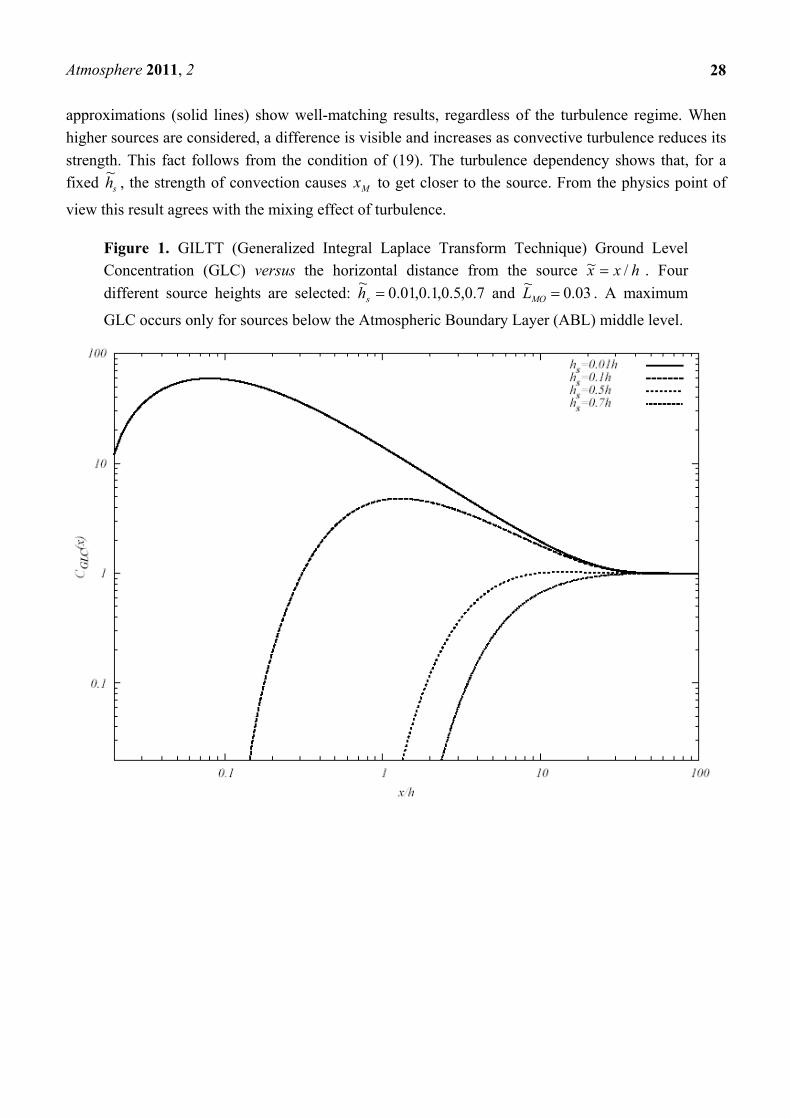
Figure 1 shows plots of the GLC versus the horizontal distance from the source x~ for near surface

source ( 01.0~sh ), a low source ( 1.0

~sh ) (at the top of the surface layer 1.0~ slz ), center source (

5.0~sh ), and high source ( 7.0

~sh ) (above ABL center) with 03.0

~0 ML . Except for the plot

7.0~sh , all show a maximum, where the sharpness of the peak reduces as sh

~ increases, until a critical

source height is reached (slightly above h5.0 ), then value 1 becomes an upper asymptote for the GLC.

When the emitting source height decreases, the maximum GLC increases, and occurs at a closer

distance, turning into a well-pronounced peak.

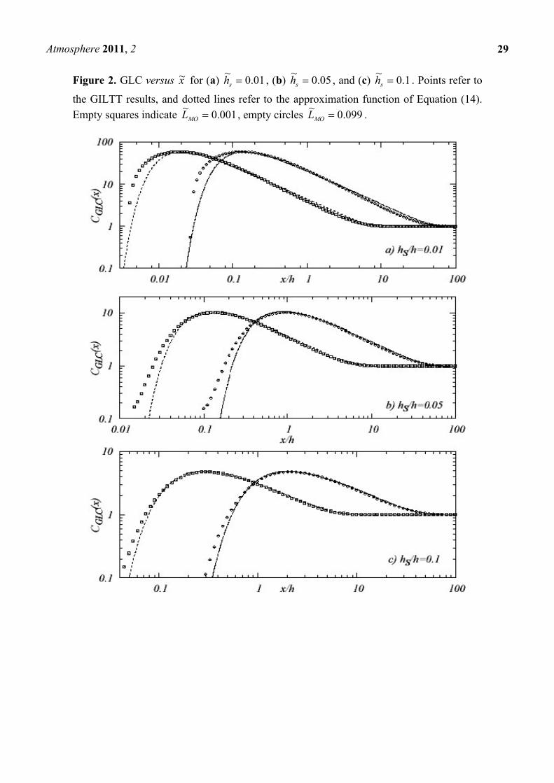
In Figure 2a–2c, the GLC versus x~ is shown for three values of sh~

( 1.0,05.0,01.0~

sh ). For each

source height, two extreme Monin-Obukhov lengths are used with 099.0 ,001.0~ MOL (empty squares

and triangles, respectively). The second value for MOL~

reflects the limit imposed by the Pleim and

Chang diffusivity introduced in Equation (6). The GILTT-based GLC are superimposed on the

approximation of Equation (14) (dotted lines). The plots show that for near surface sources there is a

slight difference between points and lines near the source position. Where the horizontal gradient is

most pronounced, a logarithmic scale enhances such a discrepancy.

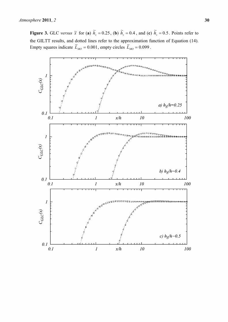
Figures 3a–3c refer to higher sources with 5.0,4.0,25.0~sh . These plots show well-matching

results as well as a good reproduction of the position where the maximum GLC occurs. As the emitting

source height sh~

increases, the approximated function slightly underestimates the GILTT-based

maximum. This discrepancy reflects the fact that condition (19) is no longer satisfied. Nonetheless,

through the whole range of source heights 25.0~

0 sh the function )(xCGLC reproduces the GILTT

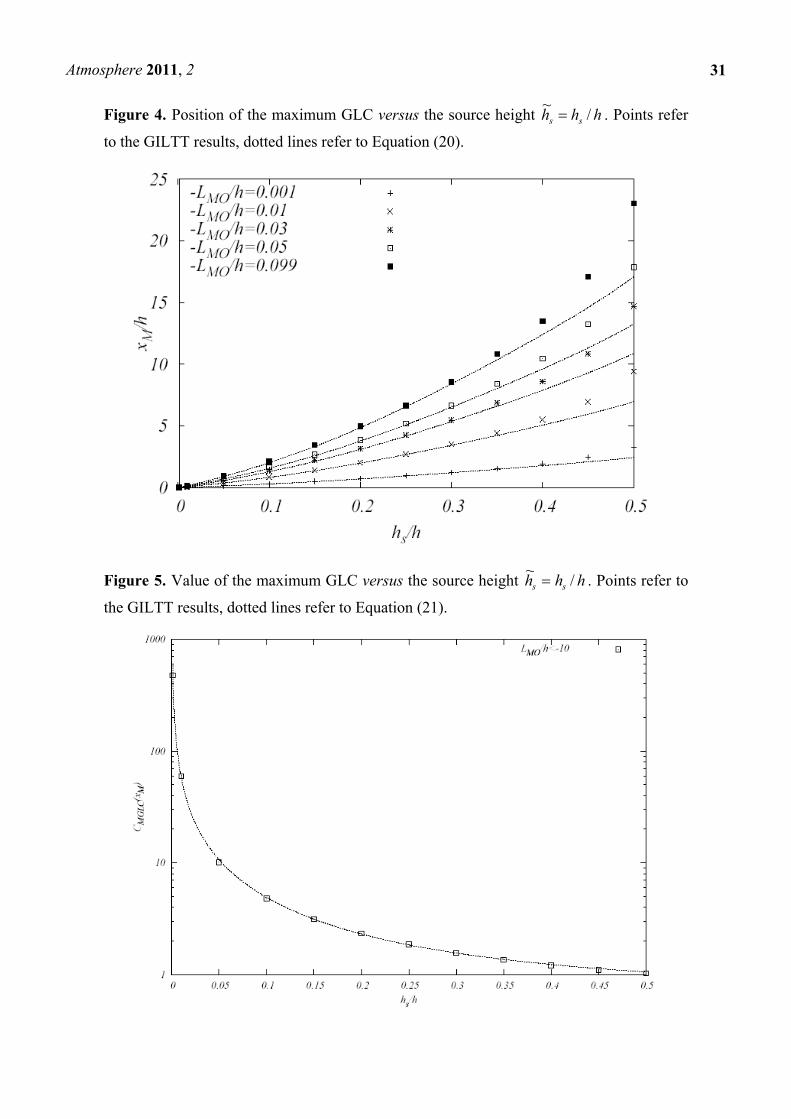
results fairly well. Figures 4 and 5 show plots of the maximum GLC )( MMGLC xC and its position Mx for several

source heights sh~

and for a selection of turbulence parameters MOL~

. In both figures the GILTT results

(points) are superimposed on the approximations (20) (dotted lines). Figure 5 depicts the position

where the maximum occurs for low sources, where GILTT results (dotted lines) and our

Atmosphere 2011, 2

28

approximations (solid lines) show well-matching results, regardless of the turbulence regime. When

higher sources are considered, a difference is visible and increases as convective turbulence reduces its

strength. This fact follows from the condition of (19). The turbulence dependency shows that, for a

fixed sh~

, the strength of convection causes Mx to get closer to the source. From the physics point of

view this result agrees with the mixing effect of turbulence.

Figure 1. GILTT (Generalized Integral Laplace Transform Technique) Ground Level

Concentration (GLC) versus the horizontal distance from the source hxx /~ . Four

different source heights are selected: 7.0,5.0,1.0,01.0~sh and 03.0

~ MOL . A maximum

GLC occurs only for sources below the Atmospheric Boundary Layer (ABL) middle level.

Atmosphere 2011, 2

29

Figure 2. GLC versus x~ for (a) 01.0~sh , (b) 05.0

~sh , and (c) 1.0

~sh . Points refer to

the GILTT results, and dotted lines refer to the approximation function of Equation (14).

Empty squares indicate 001.0~ MOL , empty circles 099.0

~ MOL .

Atmosphere 2011, 2

30

Figure 3. GLC versus x~ for (a) 25.0~sh , (b) 4.0

~sh , and (c) 5.0

~sh . Points refer to

the GILTT results, and dotted lines refer to the approximation function of Equation (14).

Empty squares indicate 001.0~ MOL , empty circles 099.0

~ MOL .

Atmosphere 2011, 2

31

Figure 4. Position of the maximum GLC versus the source height hhh ss /~ . Points refer

to the GILTT results, dotted lines refer to Equation (20).

Figure 5. Value of the maximum GLC versus the source height hhh ss /~ . Points refer to

the GILTT results, dotted lines refer to Equation (21).

Atmosphere 2011, 2

32

A final remark should be made in regard to Figure 5. Both GILTT and Equation (21) confirm that

the maximum GLC value depends on the source height, regardless of the turbulence. Based on the

Equation (21) and the parameters definitions (15)–(16) for b , c and , the leading term for the

maximum GLC results:

1~)( sMMGLC hxC (22)

where the exponent −1 is a lower bound for the source term. These results broaden the well-known

result obtained with the Gaussian approach for an unbounded ABL. Furthermore, this agrees with the

two-dimensional Gaussian result that the maximum for the GLC is:

2/12

)(

e

xC MMGLC (23)

Note that for the three-dimensional case this is no longer true. It is evident that diffusive parameters

do not play a part and it confirms that turbulence has the only effect that determines the distance where

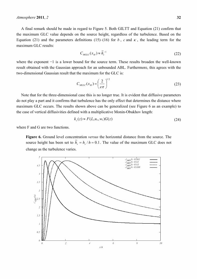
maximum GLC occurs. The results shown above can be generalized (see Figure 6 as an example) to

the case of vertical diffusivities defined with a multiplicative Monin-Obukhov length:

)(),,()( ** zGwuLFzkz (24)

where F and G are two functions.

Figure 6. Ground level concentration versus the horizontal distance from the source. The

source height has been set to 1.0/~

hhh ss . The value of the maximum GLC does not

change as the turbulence varies.

Atmosphere 2011, 2

33

7. Conclusions

The results presented in this paper show the possibility of expressing the GLC from an emitting

point-like source in a steady convective ABL by a compact analytical expression. The function was

determined analyzing the behavior of the series expansion provided by the GILTT solution, the

predictive power of which has been extensively demonstrated in the literature when applied to several

experimental data sets. Despite the simplifications due to restricting only to unstable ABL regimes, the

analysis allows a high level of understanding of the form of the ground level concentration.

The main progress worth emphasizing is the following: for a function given in Equation (14), within

the setting choice for the ABL parameter set, the maximum GLC depends only on the source height,

regardless of the Monin-Obukhov length. However, turbulence can still affect the position where the

maximum GLC occurs, which is also confirmed by the GILTT solution. A further notable point shown

in the result that no maxima occurs for all sources placed above the ABL center level; the limit

becomes an upper-bound limit. The existence of a non-zero limit is one of the main properties of the

two-dimensional ADE.

From the operative point of view, Equation (14) and its related features are useful as an additional

tool for decisional as well as emergency responses.

Acknowledgements

The authors thank Brazilian CNPq, Italian CNR and ENVIREN for the partial financial support of

this work.

References and Notes

1. Moreira, D.M.; Vilhena, M.T.; Tirabassi, T.; Buske, D.; Cotta, R.M. Near souce atmospheric

pollutant dispersion using the new GILTT method. Atmos. Environ. 2005, 39, 6289-6294.

2. Roberts, O.F.T. The theoretical scattering of smoke in a turbulent atmosphere. Proc. Roy. Soc.

1923, 104, 640.

3. Rounds, W. Solutions of the two -dimensional diffusion equation. Trans. Am. Geoph. Union 1955,

36, 395-405.

4. Van Ulden, A.P. A surface-layer similarity model for the dispersion of a skewed passive puff near

the ground. Atmos. Environ. 1992, 26A, 681-692.

5. Tirabassi T.; Rizza, U. A practical model for the dispersion of skewed puffs. J. Appl. Meteor.

1995, 34, 989-993.

6. Smith, F.B. The diffusion of smoke from a continuous elevated point-source into a turbulent

atmosphere. J. Fluid Mech. 1957, 2, 49-76.

7. Smith, F.B. Convection-Diffusion Processes below a Stable Layer; Meteorological Research

Committee N. 1048 and N. 10739: London, UK, 1957.

8. Scriven, R.A.; Fisher, B.E.A. Long-range transport of airborn material and its removal by

deposition and washout .2. Effect of turbulent-diffusion. Atmos. Environ. 1975, 9, 59-69.

9. Yeh, G.T.; Huang, C.H. Three-dimensional air pollutant modeling in the lower atmosphere.

Boundary-Lay. Meteorol. 1975, 9, 381-390.

Atmosphere 2011, 2

34

10. Berlyand, M.Y. Contemporary Problems of Atmospheric Diffusion and Pollution of the

Atmosphere; Translated version by United State Environmental Protection Agency (USEPA):

Raleigh, NC, USA, 1975.

11. Demuth, C. A contribution to the analytical steady solution of the diffusion equation. Atmos.

Environ. 1978, 12, 1255-1258.

12. Tirabassi, T.; Tagliazucca, M.; Zannetti, P. KAPPA-G, a non-Gaussian plume dispersion model:

description and evaluation against tracer measurements. JAPCA 1986, 36, 592-596.

13. Lin, J.S.; Hildemann, L.M. A generalised mathematical scheme to analytically solve the

atmospheric diffusion equation with dry deposition. Atmos. Environ. 1997, 31, 59-71.

14. Nieuwstadt, F.T.M. An analytical solution of the time-dependent, one-dimensional diffusion

equation in the atmospheric boundary-layer. Atmos. Environ. 1980, 14, 1361-1364.

15. Nieuwstadt, F.T.M.; de Haan, B.J. An analytic solution of the one-dimensional diffusion equation

in a nonstationary boundary-layer with an application to inversion rise fumigation. Atmos.

Environ. 1981, 15, 845-851.

16. Koch, W. A solution of the two-dimensional atmospheric diffusion equation with

height-dependent diffusion-coefficient including ground-level absorption, Atmos. Environ. 1989,

23, 1729-1732.

17. Abramowitz, M.; Stegun, I. Handbook of Mathematical Functions; Dover Publications, Inc.: New

York, NY, USA, 1972; p. 1047.

18. Sharan, M.; Singh, M.P.; Yadav, A.K. Mathematical model for atmospheric dispersion in low

winds with eddy diffusivities as linear functions of downwind distance. Atmos. Environ.1996, 30,

1137-1145.

19. Tirabassi, T.; Tiesi, A.; Buske, D.; Vilhena, M.T. Some characteristics of a plume from a point

source based on an analytical solution of the two-dimensional advection-diffusion equation.

Atmos. Environ. 2009, 43, 2221-2227.

20. Panofsky, H.A.; Dutton, J.A. Atmospheric Turbulence; John Wiley & Sons: New York, NY,

USA, 1988.

21. Irwin, J.S. A theoretical variation of the wind profile power-low exponent as a function of surface

roughness and stability. Atmos. Environ. 1979, 13, 191-194.

22. Pasquill, F.; Smith, F.B. Atmospheric Diffusion; John Wiley & Sons: New York, NY, USA, 1984.

23. Pleim, J.E.; Chang, J.S. A nonlocal closure.model for vertical mixing in the convective

boundary-layer. Atmos. Environ. 1992, 26, 965-981.

24. Zannetti, P. Air Pollution Modelling; Computational Mechanics Publications: Southampton, UK,

1990; p. 444.

25. Moreira, D.M.; Vilhena, M.T.; Buske, D.; Tirabassi, T. The GILTT solution of the

advection-diffusion equation for an inhomogeneous and nonstationary ABL. Atmos. Environ.

2006, 40, 3186-3194.

Atmosphere 2011, 2

35

26. Buske, D.; Vilhena, M.T.; Moreira, D.M.; Tirabassi, T. Simulation of pollutant dispersion for low

wind conditions in stable and convective planetary boundary layer. Atmos. Environ. 2007, 41,

5496-5501.

© 2011 by the authors; licensee MDPI, Basel, Switzerland. This article is an open access article

distributed under the terms and conditions of the Creative Commons Attribution license

(http://creativecommons.org/licenses/by/3.0/).