Journal of Research of the National Bureau of Standards Vol. 59, No.5, November 1957 Research Paper 2805

An Apparatus for Measurement of Thermal Conductivity of Solids at Low Temperatures

Robert 1. Powell, William M. Rogers, and Don O . Coffin

A description is given of an apparatus used for determining the t hermal conductivities o f solids in t he temperature range 4° K to 300° K. The apparatus is especially suited to the determination of thermal conductivity over a la rge temperature interval , enabling coverage of t he temperatures between t he normal boil ing points of liquefied gases. Illustrati ve results are given for an insulator, poiytetrafiuoro ethylene, and for a high-conduct ivity commerci al coalesced copper. The thermal conductivity of the insulator increases monoton­ically from 0.56 milliwatt per centimeter p er degree K at 5° K , to 2.32 at 80° K. The t hermal conductiv ity of the copper has a maximum of 24.9 watts per centimeter per degr ee K at 21 ° K , and a value of 8. 15 at 5° K. The m ethods of data analys is a nd est imat ion of errors are given.

1. Introduction

Data on thermal conductivity are neccssary for the selection of sui table construction materials, and the prediction of operating characteristics of low­temperature apparatus used in research and indus­try. In addition, accurate thermal conductivity values for pure metals and controlled alloys are important in the development and verification of theories of electronic transport phenomena in metals. The apparatus described in this paper is well suited to the measurement of thermal conductivity of metals and commercial alloys; it is also usable for poor conductors such as plastics and other dielec tric solids.

2. Experimental Apparatus

2.1. General Description

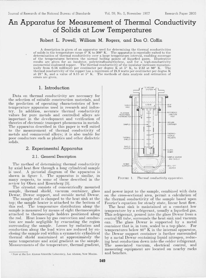
The method of determining thermal conductivity by axial heat flow through a long cylindrical sample is used. A pictorial diagram of the apparatus is shown in figure 1. The apparatus is similar, in many respects, to some of those described in the review by Olsen and Rosenberg [5].

The cryostat consists of concentrically mounted sample, thermal shield, vacuum container, glass Dewar, Dewar support, and outside metal Dewar.

The sample rod is clamped to the heat sink at the top; the sample heater is attached to the boltom of this rod . The temperature distribution along the sample is mcasured by means of eight thermocouples attached to thermocouple holders positioned along the rod. Heat losses by gas convection and conduc­tion are made negligible by evacuating the region sUlTounding the sample. Losses by radiation and conduction along the lead wires are reduced by en­closing the sample rod within a symmetric cylindrical thermal shield maintained at approximately the same temperature and axial gradient as the sample. M easurements of the temperature, thermal gradient,

1 Now at the Los Alamos Scienti fi c Laboratory, Los Alamos, New M exico.

SHIELD HEAT

RING SINK

PL ATINUM REFERENCE RESISTANCE JUNCTION

THERMOMETER POST

VACUUM SAMPLE CONTAINER

THERMO-COUPLE

THERMAL HOLDERS SHIELD

SHIELD HEATER

SAMPLE HEATER AND SHIE LD

DE WAR SUPPORT BOIL-OFF

HEATER

FI GUR E 1. Thermal conductivity appamtus.

and power input to the sample, combined with data on the cross-sectional area, permit a calculation of the thermal conductivity of the sample based upon Fourier's equation for steady state, lineal' h eat flow.

The heat sink is maintained at a constant low temperature by a refrigerant , usually a liquefied gas. This refrigerant, poured into the glass D ewar from a central fill tube, surrounds the heat sink and vacuum can. The glass Dewar is suppor ted by a metal container that is , in turn, sealed to a top plate. For temperatures below 80° Ie in the internal apparatus, the D ewar support container is further surrounded by a metal D ewar containing liquid nitrogen, reduc­ing heat conduction down into the colder refrigerant. The associated vacuum, electrical control, and measuring equipment are located on n earby racks and benches.

349

FIGURE 2. Cryostat and associated equipment.

Figure 2 is a photograph of this assembly. Two similar cryostats are used concurrcntly to increase the data output.

2 .2 . Sample Assembly

M etal and alloy sample rods are 0.367 cm in diameter and 23.2 cm long; plastic samples are 2.54 cm in diameter and 20.5 cm long. The metal and alloy rods are turned, then ground to the final diameter with a tolerance of 0.0005 cm. B ecD use of their largcr size, the plastics are turned with a toler­ance of only 0.001 cm. vVhen required, the sample is annealed after the last grinding operation. Then the thermocouple holders shown in fignre 3 arc attached, and the holders are placed on the sample with their centers 2.54 cm apart by means of gage blocks. The thermocouple holders have a thin interior edge that gives, essentially, line contact between the holder and the sample. The actual distances between flat surfaces on the holders are measured by a vernier height gage wiLh an attached precision dial test-indicator. The accuracy is aboul. 0.0005 cm. The average diameters of the samplf' are measured between the thermocouple holders to about the same accuracy.

The samples are attached to the heat sink by lL

clamping action for metals, or an internal tapered screw till'ead for plastics as is shown in figures 1 and 3. The details of the sample heaters are also in­cluded in figure 3. The heater for a metal sample is slipped onto the rod and clampcd with a small screw. In order to improve the thermal contact, mercury is placed in the hole that surrounds the lower end of the metal sample. The heater for plastic samples is screwed on so that it presses against a large copper washer used to increase the heater-to-sample con­tact area. Both heater blocks made of copper are wrapped with No. 36 or 40 AWG constantan heater wire in a single layer held in place wi th G. E. 7031

L~~ I I I I I I

~. j THERMOCOUPLE

~ BOLT

THERMOCOUPLE HOLDER

~w

METAL HEATER

AND SINK MOUNT

PLASTIC HEATER

AND SINK MOUNT

FIGURE 3. J-Ieaters and thermoccuple holders.

air-drying varnish. The sample heaters have a resistance ranging from 175 to 500 ohms for metals, and from 500 to 1,000 ohms for plastics. The power measuring circuits limit the current to a maximum of about 100 rna, and the voltage to a maximum of about 16 v. A small sample heater shield is attached to the sample by a split collet-and-serew clamp, so reducing radiation losses. These shields are covered on all exposed surfaces with aluminum foil to fur th er reduce radiation.

2 .3. Thermal Shielding, Tempering, and Controls

Several factors, such as gas conduction, radiation, and wire conduction, can lead to consistent errors in the experimental determinations of thermal con­ductivity. H eat losses by gas conduction or con­vection are reduced to an insignificant amount by baking out and evacuatin g the system to at least 10- 5 mm of H g while the system is at room tempera­ture. Cooling of the system during experimental runs further reduces the residual gas pressure.

Heat losses by radiation and lead wire conduction are greatly reduced by surrounding the sample with a cylindrical thermal shield as shown in figure l. The bottom, middle, and top of the shield are held at approximately the same temperature as the sample at the corresponding elevation . To provide a good thermal contact to the h eat sink when the shield is bolted in place, the upper shield fastening ring is made of copper . The bottom of the shield is also made of copper to provide a nearly isothermal region surrounding the sample heater. The longer inter­mediate section of the shield is made of thin stainless steel to reduce the power input necessary to maintain any given temperature gradient. The shield is split in two, vertically, to allow rota tion of the front half during the mounting and assembling of the sample.

350

The two halves are bolted together near the bottom, and a copper b ar is soldered across the bottom to im­prove thermal contact. A moun ted sample and the split shield are shown in figure 4.

Three heaters are wrapped on the shield to supply power necessary to maintain the proper thermal gra­dient. The main shield heater , wrapped back and forth across the bottom copper section, is made of 32 A WG constantan wire and has about 100 ohms re­sistance. The other two heaters at the midpoin t and near the top, made of 45 AWG constantan, have about 300 ohms resistance. All tlll'ee are kept in place with air-drying varnish. All wires connected to the sample pass through the shield and arc ce­mented to i t at areas close to the same temperature as that of their point of contact on the sample. These wires are 10 to 20 cm in length between the sample and shield .

The temperature difference between the sample heater and a horizontally opposed point on the lower copper section of the shield is measured with a gold­cobalt versus copper thermocouple. Potential differ­ences of about 0.1 J.l.v can be detected, cOl'l'esponding to from 0.02° K at liquid helium tempe'ratures, to 0.002° K at room temperature. Similar differential thermocouples are at midpoint and ncar the top .

The thermal electromotive forces developed across the middle and top differential thermocouples are measured with a d-c amplifier-galvanometer. To bring about thermal balance between the shield and sample, as indicated by null readings on the two up­per differential thermocouples, the a-c voltages sup­plied to the h eaters at the middle and top of the shield are adjusted manually. If the shield is hotter than the sample at either one of the two upper points, there is no way to obtain thermal balance. The lower, 01' m ain, differential thermocouple is th e' sensing device for a heater servomechanism. The approximately correct voltage for the bottom shield h eater is adjusted manually by varying two auto­transformers in series .

H eater and thermocouple wires arc wrapped back and forth upwards on the shield for thermal temper­ing an d then are wound on the posts attached to the heat sink. Two of the six cylindrical copper posts are shown in figUl'e 1. The winding on the posts al­lows most of the heat conducted down the wires from above to be shorted to the liquid bath. One of t he posts serves as a reference jun ction block for the eight measUl'ing thermocouples; another is used to hold a platinum resistance thermometer that indi­cates the reference temperature. The others are used for thermal tempering only.

The heat sink and posts are machined from free­cutting leaded copper , assuring both good conduc­tivity and machinability [6]. The vacuum chamber cylinder is soldered onto a lip of the heat sink with Rose's Alloy. Two thin stainless steel tubes serve as mechanical support for the internal apparatus, as exit tubes for the wires, and as pumping lines for evacua tion of the inside chamber.

For measuremen ts at liquid nitrogen, hydrogen, or helium temperatures, the entire apparatus is SUl'-

FIGU RE 4 . N/o'Unled sampLe.

rounded by liquid ni trogen in a large metal D ewar. To further reduce h eat transfer to the in ternal ap­paratus, all the wires ar c again tied down thermally to a copper post inserted into tbe pumping line just above t he top plate. The wires are brought out from the vacuum space through a hard wax seal. N ear the top of the apparatus is a thermally insu­Jated junction box where the various small wires from the cryostat are soldered to larger copper wires, usually 22 A WG, which lead to the control panel and measuring instruments.

2.4. Measuring Apparatus

The reference junction temperature for the ther­mocouples is assumed to be the same as that of the thermometer post. The measUl'ing thermometer is a strain-free capsule platinum resistor wi th an ice point resistance of about 25 ohms, which is embedded in one of the posts attached to the h eat sink. The resistance of this thermometer, calibrated down to 12° K by the T emperature M easurements Section of the Bureau, is measured on a five-dial Muell er bridge. ~When actual readings arc not being taken, this thermometer is switched to a resistance recorder. This switching allows a drift of the heat sinl;: tem-

351

1- 40 "-> , Ii

THERMOELECTRIC "..f---. POWER OF

V/ Au-2. 1 % Co vs Cu

V UJ 30 ~

~ / 0 a: t- 20 0 UJ oJ UJ 0 ~ a: 10 W

I /

/ :J: t-

I--' I/io"'" -i-"

o = I. 2 3 4 6 e 10 20 30 40 60 100 200

TEMPERATURE:K FIGURE 5. Thermocouple calibration.

perature to be observed without continual manual measurements. With liquid helium, the temperature of the heat sink is obtained from a reading of the barometric pressure by using the 1955 d compromise temperature scale [2].

Wire of 5-mil diameter , composed of gold wi th 2.1 atomic percent of cobal t, is used for the common element of the eight thermocouples [1]. The com­mon reference junction is on one post of the heat sink. The external common. lead and the separate wires going to each thermocouple JUD ction on the sample are standard thermocouple copper. The thermocouple combination was calibrated in a sep­arate apparatus. Different spools of gold-cobal t wire with the same nominal composition have been found to vary in sensitivity by about 5 to 10 per­cent. A graph of the sensitivity of the spool that was used is shown in figure 5. Each thermocouple junction has one separate external lead and is meas­ured with reference to the common junction at the heat sink. The junctions ar e electrically insulated by epo.xy resin from the thermocouple bol t and, therefore, from the holder, sample, and ground. The thermocouple leads are soldered to larger wires at the junction box. The v oltages arc read on a 5-dial vVenner potentiometer , usually to 0.01 /lV.

A determination of the power to the sample heater is obtained by measuring the d-c voltage and cur­rent. Figure 6 shows the circuit diagram. The total current passes through a calibrated I-ohm NBS- type resistor, R c; th e voltage developed across it is measured on a Rubicon type-B potenti­ometer. The effective current passes through the sample heater Rs and the lead resistances rho The currents range from several milliamperes to about 100. The voltage across the heater is divided across three calibrated resistors, arranged to give either 2 to 1 or 11 to 1 vol tage division. R esistor R3 is 10 K ohms; Rp is either 10 K ohms for 2 to 1 voltage divider ratio, or 1 K ohm for 11 to 1 ratio . The voltage, measured on the same potentiometer as the current, ranges from 1 to about 16 v. The four cal­ibrated resistors are in an oil bath maintained at 25° C by a commercial m ercury thermostat and infrared heating unit.

CRYOSTAT TERMINAL REGION BOX

1- - ------1 r -- - -l

I I I

I I II II 'I I II I II I II I II I I I I II I I I I

I: : I I _I I£.D -+ll)o. I I I • I

II II

L _ __ _ __ _ J L ___ .J

FIGURE 6.

R

H eater circuit.

Galvanometer unbalance voltages from the bridge and two potentiometers are directed to a commercial d-c breaker amplifier rather than the more commonly used moving-coil galvanometers. The input selector switch to the amplifier can be set to any of the galvanometer terminals of the bridge or potentiome­ters, or to some of the differential thermocouples between the sample and shield. The high sensitivity and several-million-fold amplification of the breaker amplifier allow interpolation one figure beyond the last dial setting on either the Mueller bridge or the Wenner potentiometer. The signal from the ampli­fi er is switched to a I-v, center zero, d-c voltmeter for precise readings, or to a slow-speed recorder for f?llowing temperature drifts or approach to equili.b­rmm.

Standard low-level electric techniques have been used: that is, all wires are s11ielcled; a special common ground wire is used ; the bridges are on insula ted ground plates; and all terminals, switches, batteries, and standard cells are thermally insulated.

2.5. Auxiliary Equipment

A pho tograph of the equipment is shown in figure 2. The vacuum control unit is behind the cryostat; the power panels and con trol are on the left. The sample space is evacuated through nominal I-in. tubes by an oil diffusion pump. Between the system and the diffusion pump is a metal cold trap that can hold liquid nitrogen over a weekend without refilling. Between the diffusion pump and the rotary mechani­cal pump is a 2-li ter reservoir that, with its valve to the mechanical pump closed, can normally hold the diffusion-pump output for 4 hI' before the pressure builds up to 100 /l . In parallel with the cold trap, diffusion pump, and reservoir, is a bypass line for pumping the system down initially without breaking the vacuum in the cold trap or diffusion pump. The pressure in the sample system is measured with a commercial ion gage when it is below 1 /l, and with a thermocouple gage when above that. The pressure in the reservoir, that is, the back pressure of the diffusion pump, is measured on another thermo-

352

couple gage system that has shutoff relays controlling the diffusion pumps and ion gage. "\Vhenever the back pressure goes above 100 Il , an alarm light turns on, and the power to the diffusion pump and ion gage turns off.

The liquid refrigcrant can be either maintained at a reduced pressure by a high-capacity mechanical pump, or vented - directly to an explosion-proof exhaust system. These ven t lines are necessary to r educe the explosion danger during liquid hydrogen tests. The vapor space over the liquid is connected to a mercury manometer, permitting measurement of the vapor pressure of the bath.

The power panel supplies both a-c and d-c voltage to the heaters and electronic equipment. The d-c voltage is obtained from a large bank of nickel­cadmium bat teries in a nearby room. The currenl through the main sample heater, which is adjusted by four variable decade re i tors, is read preliminaril y on a precision multirange milliammcter. The a-e power is obtained from a 110-v regulated power supply. Power to each of the shield heaters is con­troll ed by two autoLransformers in series. The a-c power supply also furni shes voltage to a millivolt recorder, breal er amplifier, and the main shield heater servomechanism.

2.6. Measurement Techniques

For each metal sample, the thermocouple holders are mounted in a temperature-contro ll ed shop room, where the dimensions are also measured. After these preliminary measurements, the sample is mounted in the heat sink and the heaters and thermocouples are attached. The sample is not heated or soldered after assembly of the thermocouple holders, and it is subjected to as little mechanical strain as possible during inserLion into the cryo tat. After this as­sembly, the shield is elosed and bol ted; then Lhe vacuum can is soldered in to place ,,,iLh Rose's Alloy. The sample space and tubes are evacuated and baked out for several days, usually over a weekend. The liquid refrigerants are not placed into the glass D ewar until the pressure in the cryostat is down to at least 10-5 mm of Hg.

Experimental runs are usually begun at liquid helium temperatures, after precooling first with nitrogen , then with hydrogen; and then the runs are continued at the hydrogen triple point, hydrogen boiling point, nitrogen triple point, nitrogen boiling point, carbon dioxide sublimation point, and then ice poin t. Normally, abou t six series of measure­ments at various temperature gradients are made in each temperature range. Two sets of measurements are made for each gradient to insure against reading errors or lack of steady state. The over-all tempera­ture differences across the sample vary from 10 K to a sufficiently large temperature necessary to over­lap r eadings in the next higher temperature range. The approach to steady-state conditions is observed by amplifying the unbalance emf from the Wenner potentiometer with the input switch set for the low­est thermocouple. The amplified signal is switched to the millivolt recorder, and, when this thermo-

couple emf no longer drifts with time, precise meas­urements of the voltage, current, and temperatures are begun. Measurements are also made at each sink temperaLure with no power input and with the normal vacuum space filled with helium exchange gas at a pressure of several hundred microns. Be­cause the apparatus should be isoLhermal under these conditions, these readings give the "zero" corrections for the thermocouples. These correcLions are attrib­uted primarily to inhomogeneous emf's and are assumed to be constant for a parlicular smk temperature.

Subsidiary measurements are made afterwards on a short section of the sample. They include mount­ing and polishing of the metal for photomicrographs of grain structure, measurement of hardness, meas­urement of density, and spectrographic or chemical analyses.

3. Analyses of Data

3.1. Basic Calculations

The fu ndamental equaLion of heat flow is utilized in ils differen Lial form:

Q=-XA dT dx

where Q is the heat flux, A is the lhermal conduc; tiyity, and A Lhe cross-sectional area. Because Q and A are essentially conslants of the sampl e for each run,

A d(- Qx/A). dT

Because we do not measure the temperaLure directly, but rather the Lhermocouple voltage E , we rearrange the equation to

A= d(- Qx/A) dE dE dT

where dE/dT is the thermoelectric power of Lhe thermocouple a t the given voltage E and for the given reference temperature.

Several corrections to a straightforward calculation of the heat power of the sample heater are necessary. The various componen ts of the power circuit are shown in figure 6. Basically, the power is the prod­uct of the voltage and current through the sample heater. The effective current through the heater is given by

Iell= I T- In/

where IT is the total current and In is the current through the divider circuit. The total current is given by the measmed voltage Vc across the standard resistor divided by its resistance Re. Similarly, the divider current is given by the measured divider voltage V p divided by the resistance of the particu­lar resistor R p • The effective cmrent is then

I Ve V p

ell= Rc - R p •

353

L_

The effective voltage is

V eff= p Vp- r h1efh

where rh1eff is the temperature-dependent voltage developed across the heater leads between the shield and the sample, and p is the voltage divider ratio. The ratio is given by

R1+ R2+ R3+ R p p Rp ,

where Rl and R2 are lead resistances (Rl is tempera­ture dependent), R3 is a standard 10 K ohm resistor, and Rp is either 1 K ohm or 10 K ohm.

The cross section and distances along the sample are measured at room temperature. These dimen­sions are corrected for thermal contraction at each sink temperature range whenever thermal expansion qata are available. A preliminary plot is made of Qx/A against E to check for points that arc considered to have too large a deviation. .

For the acceptable runs, the Qx/A and E are tabulated, and the values are processed by an I.BM 650 digital computer. The program fits the Qx/A data by a least squares method to polynomials to the first, second, third, and fourth degree in E. Gen­erally speaking, the first-degree polynomials give the best results for small temperature gradients, and the fourth-degree polynomials give the best for the large gradients. The computer is then programed to take the derivative of each of the polynomials, and then to multiply by the thermo­electric power of the thermocouples at each tem­perature. The final result is the thermal conduc­tivity at 1-deg intervals based upon each of the above polynomials.

Thermal conductivities as a function of tempera­ture for each run are then plotted on a large scale graph. Average or best curves are drawn through the many points for each range, and the various ranges are connected smoothly to give the complete graph.

3.2. Estimation of Errors

Three main sources of error appear in the apparatus described here: (1) Calibration of the thermocouples, (2) placement of the thermocouple holders, and (3) thermal contact resistance between the thermocouple and the sample. The first can be improved by a more complete and accurate thermocouple calibra­tion. A new series of thermocouple calibrations to improve the range and accuracy of the data has been started in thermometry calibration apparatus. The second source of error has been practically eliminated because of better control of the dimensions and place­ment of the holders. The third source of error can be reduced by increasing the length of the thermo­couple lead wire between the shield and the sample, and by obtaining better contact between the thermo­couple bolt and i ts holder.

Even after improvement, the first and third will probably remain the main sources of error. The thermocouple measurements can be improved, but appreciable errors will still come from chemical inhomogeneities, mechanical strains, uncertainty in calibration, r educed sensitivity at the lowest tem­peratures, and thermal emf in the external circuitry. The thermocouple errol' is estimated to be less than 1 percent over most of the temperature range. This error will be systematic and cannot be estimated or eliminated by statistical methods. The error caused by thermal contact resistance can be estimated by deliberately holding the thermal shield hotter or colder than the sample.

Except for gas conduction and radiation at high temperatures, the other sources of error have beeu reduced to an insignificant amount, considering the larger errors mentioned above. Errors in the cross­sectional measurements are probably about 0.2 per­cent; inaccuracy in locating the actual contact point between the thermocouple holder and sample is about the same. Errors due to radiation below 100° K and conduction along lead wires were calc­ulated to be below 0.1 percent. To check these radiation losses at higher temperatures, several trial runs with different gradients were made at the ice point. Apparently, for metals, an error of about 1 to 2 percent exists in the readings at that tempera­ture as disclosed by a systematic dependence of the apparent conductivity on the gradient. Several runs were made with a residual helium gas pressure of approximately 1 X 10- 5 mm Hg within the system. These runs differed by about 3 percent for most temperatul'e ranges .

Experimental runs in each temperature range have been analyzed for internal consistency. The devia­tions from an average curve are usually less than 1 percent in the liquid helium and hydrogen ranges, and less than }6 percent at liquid nitrogen tempera­tures and above. These inconsistencies are ap­parently due to the combined result of the various errors mentioned above, the one exception being thermocouple calibration error, which is systematic. The inaccuracies increase if the sample has ei ther a very high or a very low conductivity. The range of usable sample diameters is not as great as the variation in conductivity; therefore, at both ex­tremes of conductivi ty, optimum measuring con­ditions cannot be obtained. Recent measurements on a very pure copper sample that had a conductivity maximum over 100 w/cm oK gave inconsistencies of about 5 percent between 4° K and 60° K. Measure­ments on very low conductivity alloys or plastics have about this same inaccuracy, and, in addition, arc usually not reliable above 100° K because of the increasing significance of radiation exchange be­tween the sample and shield.

Many control experiments have been carried out to test the self-consistency of the apparatus. Many of the runs overlap in temperature range. For example, some of the runs were carried out with the heat sink at 4° K and the bottom of the sample

354

around 25° K, thus overlapping runs made with the sink at 19.7° K. The conductivity curves from the lower ranges fit smoothly with the curves at the higher tempemtures. Apparent conductivities from runs with diffeTent thermal gradients on the sample usually agree within the scatter normally character­istic of a single run. Various runs with different size samples and holders gave consistent results.

4. Results

4 .1. Polytetrafluoroethylene

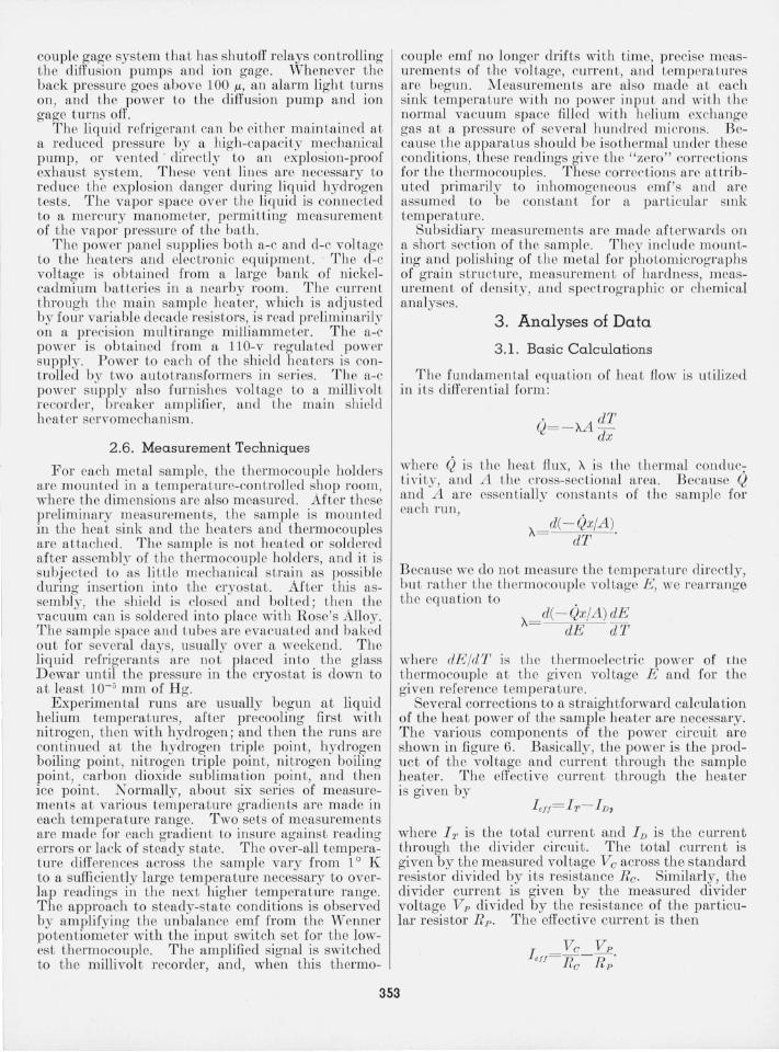
The graph of thermal conductivity of this plastic is given in figure 7. The estimated inaccuracy of the results is about 10 percent. The sample was ex­truded and had a density of 2.218 g/cm3 • Thermal contraction vvas calculated by using the data of Quinn, et a!. [7] for the higher temperatures, and the data of Head and Laquer [3] for the low tempera­tures [4].

2. 5 ---- -

2_ 0 -

--- --- -- -

f-- i--51- ---

t f----f--i-- /

V -o - f- -

4--0

I- i- VI - -01- ~j 1 t-------

0

.6

_5 '0

- I--- ..<

" ~ 7

/

~7

~ - ---

----

--I- -I-

-

t-- ~

20 TEMPERATURE, CI K

-

-

40

-/"

60 80 100

FIGURE 7. Thermal conductivity of poiytetTajluoroethylene. (The dashed lines indicate interpolated regions.)

4.2. Coalesced Copper

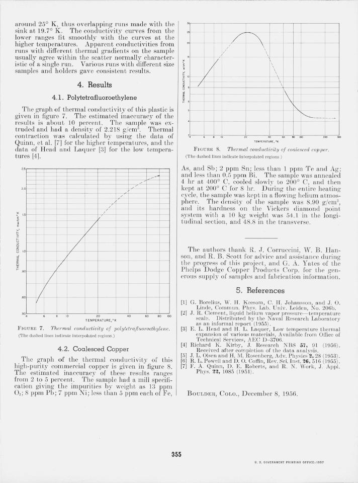
The graph of the thermal conductivity of this high-purity commercial copper is given in figure 8. The estimated inaccuracy of these results ranges from 2 to 5 percent. The sample had a mill specifi­cation giving the impurities by weight as 13 ppm O2 ; 8 ppm Pb; 7 ppm Ni; less than 5 ppm each of Fe,

1

,, -

"/ ~, -

20 - t-- t- -/

" \ / / \ :-J \ -

\ \ \ \

I-- - , i-\ -~ j--I - ---- I--\

B

.- -- t- r\ ~

, l- t- t- -

, --- 1"-1'---------

' I--- ~ -

, . 0 ., '00 200

TE MPERATURE, -I(

FIGUHE 8. Thermal conductivl:ty (Jf coalesced cop pel'. (The dashed lines indicate in te rpola ted regions)

"'"

As, and Sb; 2 ppm Sn; less than 1 ppm Te and Ag; and less than 0.5 ppm Bi. The sample was annealed 4 hr at 400 0 C, cooled slowly to 200 0 C, and then kept at 200 0 C for 8 hI". During the entire heating cycle, the sample was kept in a f-lowing helium atmos­phere. The densi ty of the sample was 8.90 g/cm3,

and its hardness on the Vickers diamond point system with a 10 kg weight was 54 .1 in the longi­tudinal section, and 48.8 in the transverse.

The authors thank R. J. COlTucci ni , W·. B. Han­SOil, and R. B. Scott for advice and assistance during the progress of this project, and G. A. Yates of the Phelps Dodge Copper Products Corp. for the gen­erous supply of samples and fabricatio n information.

5. References

[1] G. Borelius, IV. I-I. K eesom, C. H . Johansson, and J. O. Linde, Commun. Phys. Lab . Univ. Leiden, No . 206b.

[2] J. R. Clement, liquid helium vapor pressure- temperature scale. Distributed by the Naval Research Laboratory as an informal report (1955) .

[3] E. L. H ead and H. L. Laquer, Low temperature t hermal expansion of various materials, Available from Office of Technical Services, AEC D -3706.

[4] Richard K. Kirby, J . Research N BS 57, 91 (1956) . Received after comple tion of the data analysis.

[5] J. L. Olsen and H. M. Rosenberg, Adv. Physics 2, 28 (1953) . [6] R. L. Powell and D. O. Coffin, Rev. Sci. Inst. 26, 516 (1955) . [7] F. A. Quinn, D. E. Roberts , and R. N. Work, J . App!.

Phys. 22, 1085 (1951).

BOULDER, COLO., December 8, 1956.

355 U, S. GOVERNMENT PRINTING OFFICE: 1957