an automated process for concrete reinforcement layout …
TRANSCRIPT

IN DEGREE PROJECT THE BUILT ENVIRONMENT,SECOND CYCLE, 30 CREDITS
, STOCKHOLM SWEDEN 2018
An Automated Process for Concrete Reinforcement Layout Design
CECILIA GAVRELL
LUDVIG REUTERSWÄRD
KTH ROYAL INSTITUTE OF TECHNOLOGYSCHOOL OF ARCHITECTURE AND THE BUILT ENVIRONMENT
An Automated Process for ConcreteReinforcement Layout Design
MSc Thesis in Structural Engineering and BridgesKTH Royal Institute of Technology
CECILIA GAVRELL & LUDVIG REUTERSWÄRD
Master’s Thesis at ABESupervisors: Christo�er Svedholm, Raid Karoumi and Johan Ganebo
Examiner: Costin Pacoste
TRITA-ABE-MBT-18301

iii
Abstract
As many tasks considering structural design in civil engineering becomedigitalised, the possibility of creating a more e�ective workflow increases. Thedevelopment of computer programs that can handle large amounts of data andassist the decision making during design process increases the requirement ofthe data management to fully utilize the potential of a digital workflow. Thedesign of reinforcement layout of concrete structures is time demanding andoften performed manually. These characteristics of a workflow indicates thatit may be suitable to be subject to automation.
The aim of this thesis is to highlight the potential and the di�culties ofusing automated design procedures in civil engineering with focus on reinforce-ment layout design. Specifically, the selection of straight rebars and their place-ment within concrete structures has been studied with respect to buildabilityand the amount of reinforcement used.
A computer program has been developed to select rebar diameters andarrangement, satisfying the required amount of reinforcement as well as someof the rules according to the Eurocode standard. In order to find feasiblesolutions, an optimization of the amount of reinforcement as well as di�erentmeasures of buildability is performed, using a genetic algorithm.
The result from two case studies showed that the program managed toperform tasks similar to an engineer and create design solutions which reducedthe amount of reinforcement and the number of rebar types. Furthermore, itwas shown that consideration to the identified buildability parameters playedan important role in finding an optimal solution. The findings indicate thatthe design of reinforcement layout may be automated and that a more e�ectiveworkflow can be achieved.
Keywords: genetic algorithm, optimization, reinforcement layout design,automation, buildability, constructability
iv
Sammanfattning
I takt med att fler delar av projekteringen av anläggningskonstruktioner blirdigitaliserade ökar möjligheterna för att e�ektivisera arbetet. Utvecklandet avdatorprogram som kan hantera mycket information och ge stöd till beslutsfat-tande ställer också krav på hanterandet av denna data för att utnyttja denfulla potentialen av ett digitaliserat arbetsflöde. Arbetsprocessen vid armeringav betongkonstruktioner är tidskrävande och utförs idag ofta helt eller delvisför hand. Sådana processer bär karaktärsdrag som tyder på att de är lämpadeför automatisering.
Målet med studien är att undersöka problematiken kring att automatiseraarbetsprocesser vid projektering av anläggningskonstruktioner med inriktningpå armering av betongkonstruktioner. Specifikt, så har valet av raka arme-ringsjärn och dess placering i betongkonstruktioner studerats med avseende påbyggbarhet och armeringsmängder.
Ett datorprogram har utvecklats för att välja armeringsjärn och dess pla-cering för ett givet behov och ett antal krav som ställs enligt Eurokod. För atthitta en möjlig lösning är problemet formulerat som en optimering av arme-ringsmängd och olika mått på byggbarhet. Optimeringen genomfördes med engenetisk algoritm.
Resultatet från två fallstudier visar att programmet lyckades genomförakonstruktörens arbetsuppgifter och skapa lösningar som minskade mängdenanvänd armering och antalet olika typer av armeringsjärn samtidigt som deidentifierade måtten på byggbarhet främjades. Vidare visade resultatet att deidentifierade byggbarhetsparametrarna spelade en viktig roll för att finna enoptimal lösning. Detta indikerar att det är möjligt att automatisera dennaprocess och att ett e�ektivare arbetsflöde kan erhållas.
Nyckelord: genetisk algoritm, optimering, armering, automatisering, bygg-barhet

Preface
This master thesis was written for the Department of Civil and Architectural En-gineering, the division of Structural Engineering and Bridges at the Royal Instituteof Technology (KTH) during the spring of 2018.
First and foremost, we would like to express our gratitude to our supervisorPh.D. Christo�er Svedholm at ELU Konsult AB for showing great enthusiasm,encouragement and guidance throughout our thesis work.
We also would like to thank our supervisors Prof. Raid Karoumi at the Divisionof Structural Engineering and Bridges at KTH and Johan Ganebo at ELU KonsultAB who provided various perspectives and feedback on our work.
Last but not least, our deepest gratitude to ELU Konsult AB for giving us theopportunity to write our master thesis at their o�ce in Stockholm and lending usmaterial for the performed case studies.
Stockholm, June 2018
Cecilia Gavrell and Ludvig Reuterswärd
v
Contents
Abstract iii
Sammanfattning iv
Preface v
List of Symbols vii
1 Introduction 1
1.1 Aim . . . . . . . . . . . . . . . . . . . . . . . . . . . . . . . . . . . . 21.2 Scope . . . . . . . . . . . . . . . . . . . . . . . . . . . . . . . . . . . 21.3 Outline of the Thesis . . . . . . . . . . . . . . . . . . . . . . . . . . . 2
2 Background 3
2.1 Concrete Reinforcement Layout Design . . . . . . . . . . . . . . . . . 32.1.1 The Process of Choosing Rebar Types and Placement . . . . 3
2.2 Buildability . . . . . . . . . . . . . . . . . . . . . . . . . . . . . . . . 52.2.1 Buildability Factors in the Reinforcement Design Process . . 7
2.3 Design Practice in Structural Engineering . . . . . . . . . . . . . . . 72.3.1 Point Based Design . . . . . . . . . . . . . . . . . . . . . . . . 72.3.2 Set Based Design . . . . . . . . . . . . . . . . . . . . . . . . . 8
2.4 Automated Design in Civil Engineering . . . . . . . . . . . . . . . . 92.4.1 The Reinforcement Design Process and BIM . . . . . . . . . 9
2.5 Optimization . . . . . . . . . . . . . . . . . . . . . . . . . . . . . . . 102.5.1 The Optimization Process . . . . . . . . . . . . . . . . . . . . 112.5.2 Discrete Variable Optimization . . . . . . . . . . . . . . . . . 122.5.3 Genetic Algorithms . . . . . . . . . . . . . . . . . . . . . . . . 12
3 Method 15
3.1 Constructing the Program . . . . . . . . . . . . . . . . . . . . . . . . 153.1.1 Program Outline . . . . . . . . . . . . . . . . . . . . . . . . . 153.1.2 Module 1 . . . . . . . . . . . . . . . . . . . . . . . . . . . . . 173.1.3 Module 2 . . . . . . . . . . . . . . . . . . . . . . . . . . . . . 203.1.4 Module 3 . . . . . . . . . . . . . . . . . . . . . . . . . . . . . 22
vi
CONTENTS vii
3.2 Model Validation . . . . . . . . . . . . . . . . . . . . . . . . . . . . . 273.2.1 Convergence Check . . . . . . . . . . . . . . . . . . . . . . . . 273.2.2 Parameter Sensitivity . . . . . . . . . . . . . . . . . . . . . . 28
3.3 Case Study . . . . . . . . . . . . . . . . . . . . . . . . . . . . . . . . 293.3.1 Case 1 - Cirkulationen, Arenastaden . . . . . . . . . . . . . . 303.3.2 Case 2 - Slussen . . . . . . . . . . . . . . . . . . . . . . . . . 31
4 Results 33
4.1 Model Validation . . . . . . . . . . . . . . . . . . . . . . . . . . . . . 334.1.1 Convergence Check Module 1 . . . . . . . . . . . . . . . . . . 334.1.2 Convergence Check Module 3 . . . . . . . . . . . . . . . . . . 364.1.3 Parameter Sensitivity Module 1 . . . . . . . . . . . . . . . . . 384.1.4 Parameter Sensitivity Module 3 . . . . . . . . . . . . . . . . . 40
4.2 Case study 1 - Cirkulationen, Arenastaden . . . . . . . . . . . . . . . 424.3 Case Study 2 - Slussen . . . . . . . . . . . . . . . . . . . . . . . . . . 48
5 Discussion and Conclusions 53
5.1 Discussion . . . . . . . . . . . . . . . . . . . . . . . . . . . . . . . . . 535.2 Conclusions . . . . . . . . . . . . . . . . . . . . . . . . . . . . . . . . 555.3 Future Research . . . . . . . . . . . . . . . . . . . . . . . . . . . . . 55
Bibliography 57
A Case study 1 - Cirkulationen 61
A.1 Parameter Sensitivity Case 1 . . . . . . . . . . . . . . . . . . . . . . 61A.1.1 Top Flexural Reinforcement, Direction 1 . . . . . . . . . . . . 61A.1.2 Bottom Flexural Reinforcement, Direction 1 . . . . . . . . . . 63A.1.3 Top Flexural Reinforcement, Direction 2 . . . . . . . . . . . . 65A.1.4 Bottom Flexural Reinforcement, Direction 2 . . . . . . . . . . 67
B Case Study 2 - Slussen 71
B.1 Parameter Sensitivity Case 2 . . . . . . . . . . . . . . . . . . . . . . 71B.1.1 Top Flexural Reinforcement, Direction 1 . . . . . . . . . . . . 71B.1.2 Bottom Flexural Reinforcement, Direction 1 . . . . . . . . . . 73B.1.3 Top Flexural Reinforcement, Direction 2 . . . . . . . . . . . . 76B.1.4 Bottom Flexural Reinforcement, Direction 2 . . . . . . . . . . 78


List of Symbols
–
c
Objective function weight considering rebar centre-to-centre distance. [≠]
–
g
Objective function weight considering the number of rebar subgroups. [≠]
–
„
Objective function weight considering the number of rebar dimensions. [≠]
–
l
Objective function weight considering the number ofreinforcement levels. [≠]
–
v
Objective function weight considering the total amount of reinforcement. [≠]
‰ Decision variable. [≠]
≥p
Data structure containing all combinations of reinforcement levels. [≠]
„ Nominal rebar diameter. [mm]
„
p
Data structure containing all combinations of rebar dimensions. [mm]
Á
N
Percentage di�erence in number of di�erent reinforcement barsbetween optimization algorithm and hand calculations. [%]
Á
Q
Percentage di�erence in quantity between optimization algorithmand hand calculations. [%]
˛u
max
Vector containing maximum coordinates of L. [m]
˛u
min
Vector containing minimum coordinates of L. [m]
A Area of unadjusted rebar group polygon. [m2]
A
Õ Area of adjusted rebar group polygon. [m2]
A
s
Total reinforcement cross-section area per meter. [mm2/m]
A
cell
Area of node cell. [m2/m]
A
s,req,max
Maximum required reinforcement. [mm2/m]
A
s,req
Required reinforcement. [mm2/m]
ix
x CONTENTS
A
tot
Surface area of the structure. [m2]
B Boundary polygon of the vertices of L. [m2]
B
Õ Adjusted boundary polygon of the vertices of L
Õ. [m2]
c Centre-to-centre distance of rebars. [m]
C
u
Contour polyline in the u-plane. [m]
C
z
Contour polygon in the z-plane. [m]
c
max
Maximum centre-to-centre distance of rebars. [m]
L Group of contour intersection lines. [m]
L
Õ Adjusted group of contour intersection lines. [m]
N Number of di�erent types of reinforcement bars. [pcs]
n
„,max
Maximum number of rebar diameters. [pcs]
n
„
Number of rebar diameters. [pcs]
n
g,tol
Rebar subgroup size tolerance. [≠]
n
g
Number of rebar subgroups. [pcs]
n
l,max
Maximum number of reinforcement levels. [pcs]
n
layer
Number of reinforcement layers. [pcs]
n
l
Number of reinforcement levels. [pcs]
Q Amount of reinforcement [kg/m3]
S Surface interpolation of x, y, z [mm2/m]
u Direction parallel to the reinforcement. [m]
V Volume under surface S [m3]
v Direction perpendicular to the reinforcement. [m]
V
Õ Volume under adjusted surface S
Õ [m3]
V
max
Volume under the adjusted surface S
Õmax
[m3]
x Spatial coordinate. [m]
y Spatial coordinate. [m]
Chapter 1
Introduction
The design of concrete reinforcement layout is a cumbersome task. The amount ofinterdependent variables and constraints that has to be evaluated renders a iterativedesign process that is di�cult to oversee. In the design process, the possibility to in-fluence the final results are greater in an early phase while the available informationto base the decision on is sparse (Horn, 2015).
The reinforcement layout design is evaluated by assuming a specific dimensionand center distance between the rebars based on the required reinforcement inthe structure and the experience gathered from earlier projects. If the solution issatisfactory from a structural engineers point of view, the solution will be givento the contractor for evaluation. Thus, the contractor has one solution to choosefrom. This design methodology can be referred to as a point-based design. Possiblesolutions that may be optimal for other parts of the project may already havebeen discarded at this point. In order to to avoid this problem a set-based designmethodology can be used (Parrish et al., 2007). The main idea is to keep as manypossible solutions in the project for as long as possible to be able to make the decisionwhen the available information to find an optimal solution is greater (Horn, 2015).With such a design methodology multiple solutions are presented to the contractorand a solution that is considered optimal for both parties can be chosen.
The obvious problem with the set based design methodology is coupled withthe possibility to generate multiple solutions. Automatization of the design processhas been used in other areas of civil engineering to provide a method for generatingsolutions quickly. Techniques of solving non-linear optimization problems of discretevariables such as in genetic algorithms (GA) are commonly used.
Another di�culty is that the optimal solution is di�cult to define. Parameterssuch as the number of allowed di�erent types of reinforcement, the building orderand other buildability issues vary dependent on the project and contractor. Thissomewhat arbitrary objective has to be handled simulating human decision making.
1
2 CHAPTER 1. INTRODUCTION
1.1 AimThe aim of this thesis is to highlight the potential and the di�culties of using auto-mated design procedures in civil engineering with a focus on reinforcement layoutdesign. Di�erent measures of how to consider buildability in reinforcement layoutdesign and how these measures influence the amount of reinforcement material usedare evaluated.
1.2 ScopeThe work in this thesis is mainly focused on reinforced concrete slab structureswith straight reinforcement bars. To limit the scope of the study, corner detailing,openings in the geometry and structural connections will not be considered.
A new methodology for implementation of an automated design process is de-veloped. The approach includes using an optimization algorithm, programmed inMatlab, to minimize the amount of reinforcement used and optimize of the choice ofreinforcement bars. Previously calculated required reinforcement for the envelopeof all load combinations will be used as input data in the developed optimizationalgorithm, where the required reinforcement was calculated from section forces inin a Finite Element (FE) solver. The optimization algorithm will construct layoutsfor top and bottom flexural reinforcement in two directions.
Since this methodology is to be used as an aid in the design process, case studieswill be performed to validate the developed algorithm with regard to buildabilityas well as its ability of performing a task similar to an engineer.
1.3 Outline of the ThesisThe first chapter gives an introduction to this thesis. In chapter 2, a theoreticalbackground to the concepts discussed in this thesis is given and an introduction tothe specific problem studied. In chapter 3, a methodology for automation of concretereinforcement layout design is presented, as well as the procedure of measuringbuildability and performing the case studies. In chapter 4, the results are presentedand in chapter 5, conclusions are drawn from the results.
Chapter 2
Background
2.1 Concrete Reinforcement Layout DesignThe design of reinforced concrete elements is a process consisting of several steps.To perform some of the steps, assumptions regarding the final design must be madein order to perform the calculations. This is rendering an iterative procedure wheresome of the steps might have to be repeated to find a satisfactory design. Firstly,the geometry and the loads are defined. The sectional forces are then calculated, aswell as the required reinforcement. A set of rebar elements are chosen based on ex-perience and then placed to fulfill the design requirements. This task is cumbersomeand therefore it is possible that only one or few design alternatives are explored.Once the rebar placement is defined, reinforcement design drawings or 3D-modelsare made. An elaboration on the design process is presented is Section 2.4.1.
2.1.1 The Process of Choosing Rebar Types and Placement
Reinforcement design of structural concrete elements is performed considering theultimate limit state, serviceability limit state, fatigue and crack control. Calcula-tions of required reinforcement in ultimate limit state are carried out by assum-ing some placement of the reinforcement bars and then, from a static equilibriumbetween the loading and the resistance, the required amount of reinforcement isderived.
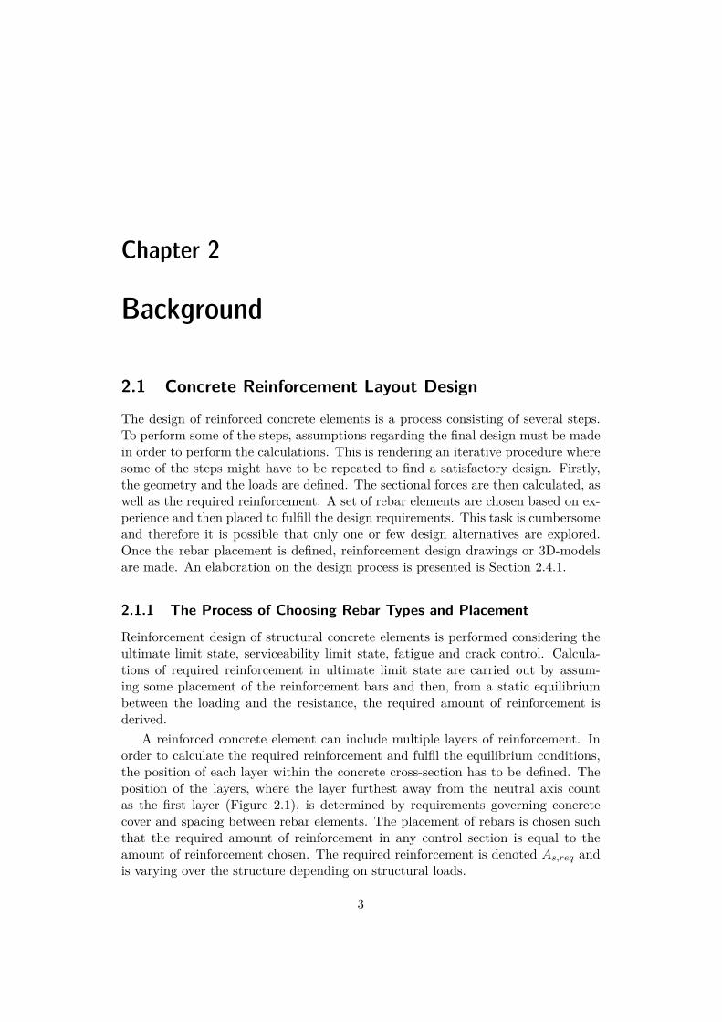
A reinforced concrete element can include multiple layers of reinforcement. Inorder to calculate the required reinforcement and fulfil the equilibrium conditions,the position of each layer within the concrete cross-section has to be defined. Theposition of the layers, where the layer furthest away from the neutral axis countas the first layer (Figure 2.1), is determined by requirements governing concretecover and spacing between rebar elements. The placement of rebars is chosen suchthat the required amount of reinforcement in any control section is equal to theamount of reinforcement chosen. The required reinforcement is denoted A
s,req
andis varying over the structure depending on structural loads.
3
4 CHAPTER 2. BACKGROUND
Layer 2Layer 1
M
FC
N.L
FS,1
FS,2
M
Figure 2.1: Position of reinforcement layers.
The chosen amount of reinforcement is calculated according to Eq. (2.1) whichis the total cross section area of the rebars per meter in a section perpendicular tothe reinforcement direction. The main objective is to find a combination of rebardimensions and spacing that matches A
s,req
in every point of the structure. However,the rebar dimensions are limited to available stock sizes and the rebar spacing islimited due to buildability reasons. Furthermore, individual rebar elements must besorted on site and the number of di�erent elements will render a more complicateddesign.
A
s
= fi„
2
41c
(2.1)
In this thesis, a reinforcement level is defined as a combination of reinforcementdiameter „ and centre-to-centre distance c. Reinforcement levels may be combineduntil the required amount of reinforcement is exceeded by the sum of the chosenreinforcement levels. However, the total amount of reinforcement levels must fitwithin the maximum number of layers, regarding rebar spacing limitations.
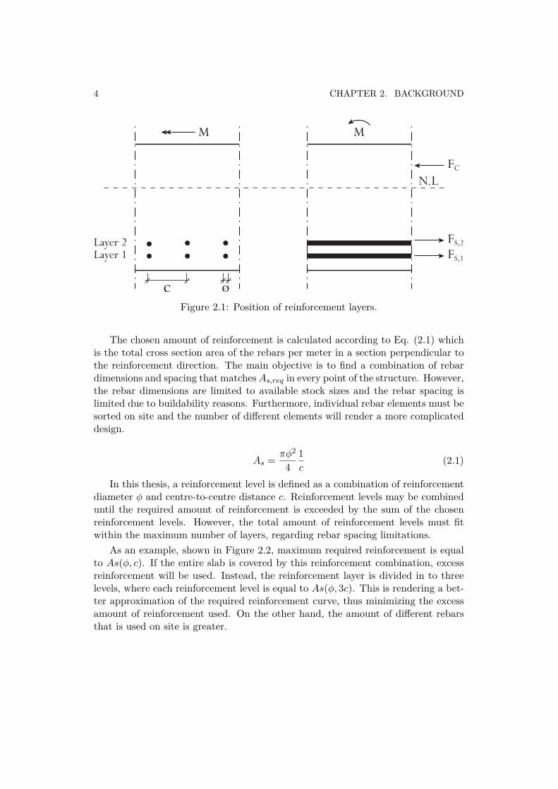
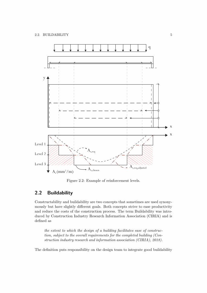
As an example, shown in Figure 2.2, maximum required reinforcement is equalto As(„, c). If the entire slab is covered by this reinforcement combination, excessreinforcement will be used. Instead, the reinforcement layer is divided in to threelevels, where each reinforcement level is equal to As(„, 3c). This is rendering a bet-ter approximation of the required reinforcement curve, thus minimizing the excessamount of reinforcement used. On the other hand, the amount of di�erent rebarsthat is used on site is greater.
2.2. BUILDABILITY 5
q
y
x
Level 1
Level 2
Level 3
As,req
As,req,adjustedAs,chosenAs (mm2/m)
x
Figure 2.2: Example of reinforcement levels.
2.2 BuildabilityConstructability and buildability are two concepts that sometimes are used synony-mously but have slightly di�erent goals. Both concepts strive to ease productivityand reduce the costs of the construction process. The term Buildability was intro-duced by Construction Industry Research Information Association (CIRIA) and isdefined as
the extent to which the design of a building facilitates ease of construc-tion, subject to the overall requirements for the completed building (Con-struction industry research and information association (CIRIA), 2018).
The definition puts responsibility on the design team to integrate good buildability
6 CHAPTER 2. BACKGROUND
in the design. The term constructability, on the other hand, was introduced by theConstruction Industry Institute (CII) and is defined as
the e�ective and timely integration of construction knowledge into theconceptual planning, design, construction, and field operations of a projectto achieve the overall project objectives in the best possible time and ac-curacy at the most cost-e�ective levels (Construction Industry Institute(CII), 2018).
The definition of constructability emphasises on management and includes allstages of the building process (Lam et al., 2005). This thesis concerns the influencethat the design team has on the ease of construction. Therefore the term buildabilitywill be used even though literature about both concepts will be explored.
Many studies have confirmed a positive relationship between improved buildabil-ity and cost- and time savings, safety, labour productivity and quality performance.The ability to influence buildability aspects in the design, decreases rapidly as theproject progresses to a stage when decisions become more detailed and the ability toinfluence the final design gets limited. Therefore, it is crucial to consider buildabil-ity aspects in an early stage of the design process, when important design changesare being executed (Lam et al., 2005).
The traditional design approach separates design from construction so that theengineer and the contractor have di�erent areas of responsibilities, e.g. the engi-neer will focus on finding a structurally sound design that the contractor later willproduce. If there is little communication between the engineer and the contractor,buildability aspects may not be considered in the design stage, which in turn canlead to project delays, ine�cient use of resources, reworks, schedule interruptionsand cost overruns (Lam et al., 2005). Not considering buildability in the designstage of a reinforced concrete construction may lead to a design that includes com-plicated fixing methods and connection details that significantly increase the timeworkers have to spend on bending and fixing the reinforcement bars and constructthe formwork (Simonsson, 2011).
One important factor for implementation of buildability in the design processis how to quantify buildability and select an appropriate method for integration ofbuildability. Using questionnaire surveys is a common method to quantify build-ability. Simonsson (2011) performed a questionnaire survey, targeting respondentswithin the Swedish civil engineering construction industry. The respondents in-cluded participants from contractor and designer firms and the Swedish transportadministration (Trafikverket). The survey showed that the top five factors a�ectingbuildability of civil engineering projects are early involvement of contractor, work-place organization, available space on construction site, production planning andprefabrication of reinforcement. Furthermore, the survey showed that contractorshave the least opportunity to influence buildability while designers and clients havethe most.
2.3. DESIGN PRACTICE IN STRUCTURAL ENGINEERING 7
Most studies found in the literature give guidelines of what to consider through-out the design and construction phase. The thesis by Horn (2015), on the otherhand, focuses on including buildability early on in the design phase by establishingquantifiable design metrics. By generating a large sample of designs for steel trussfacade structures and evaluating the designs according to quantifiable structuralperformance and buildability metrics, it was shown that there was a significanttrade-o� between the two metrics. The study lay grounds for investigation andapplication of similar metrics to various other structural elements and materials.
2.2.1 Buildability Factors in the Reinforcement Design ProcessThe main focus of this thesis is implementation of buildability early on in the designprocess of reinforced concrete structures. In the available literature, the followingfactors have been suggested to a�ect buildability of a reinforced concrete structure:
• Recurrence of reinforcement bars (Tauriainen et al., 2015). Stock lengths andstock dimension of bars should be used when possible (Concrete ReinforcingSteel Institute (CRSI), 2013).
• Dimension of reinforcement bars. Large dimensions of reinforcement barsshould be favored instead of small whenever it is possible (Tauriainen et al.,2015) since placing and fabrication costs are minimized by using the largestpractical bar sizes while still meeting the design requirements (Concrete Re-inforcing Steel Institute (CRSI), 2013).
• General placement of main reinforcement bars (Tauriainen et al., 2015).
• Distance between bars. Dense reinforcement bar mountings should be avoidedto facilitate compaction work (Tauriainen et al., 2015) and pouring of concrete(Simonsson, 2011).
• Geometric shape of bars. Straight reinforcement bars should be used whereverpossible because fabricating and placing straight bars is faster and easier thanbent bars (Concrete Reinforcing Steel Institute (CRSI), 2013).
The factors above will be incorporated into the optimization algorithm developedin this thesis in order to take buildability into account.
2.3 Design Practice in Structural Engineering2.3.1 Point Based DesignThe traditional design approach of structural design of concrete structures followsa point-based design methodology. A point-based design involves choosing a singlestructurally feasible option in the solution space at each step of the design process.
8 CHAPTER 2. BACKGROUND
The chosen option is then modified and refined in an iterative process until it is sat-isfactory from a structural point of view. Even though a point-based methodologycan render a technically feasible and structurally sound solution, it may not takeother factors, for example buildability, into account since the expertise of those whoperform the actual labour have not been included in the design (Parrish et al., 2007).Another disadvantage with a point-based design method is that it is mainly basedon a trial and error method, e.g. if a feasible solution is not found or backgroundconditions are changed, many iterations may be needed to backtrack and refine thesolution (Ward et al., 1995). Furthermore, the structural engineer is required tomake decisions in the early stages of the design process, unknowing of how it willa�ect the final outcome (Parrish et al., 2007).
2.3.2 Set Based Design
In contrast to point-based design a set-based design methodology makes it possibleto delay certain design decisions and consider a broader range of possible solutions.When using a set based approach, sets of possible solutions are broadly consideredin the initial phase and then gradually narrowed down, eliminating weaker solutions,until a final globally optimal solution is chosen (Parrish et al., 2007). A set baseddesign approach allows for greater parallelism in the design process and explorationof the space of possible designs before making important decisions, which minimizesthe risk for rework (Sobek II et al., 1999). Furthermore, it allows for communicationbetween the design team and other project participants, which can be an importantfactor for finding a solution that is optimal for all involved participants. By includingthe expertise and knowledge of for example contractors early on in the design processand by making sure that the chosen sets of solutions are compatible with theirpreferences, the final solution will most likely not only be a technical feasible solutionbut also be a buildable solution (Liker et al., 1996; Parrish et al., 2007).
The concept of set-based design was introduced in the late 1980s by Ward andSeering and is described in their work Quantitative Inference in a Mechanical Design"Compile" (Ward and Seering, 1989). Further development of the concept andestablishment of the principles of the set based design is presented in the articleToyotas Principles of Set-based Concurrent Engineering by (Sobek II et al., 1999).The authors suggested three basic principles for implementation of a set baseddesign: (1) map the design space, (2) integrate by intersection, and (3) establishfeasibility before commitment. The first principle involves defining feasible regions,designing multiple alternative solutions, exploring trade-o�s and communicatingpossibilities. The second principle includes looking for intersections of feasible sets,impose minimum constraints and seek conceptual robustness. The last principlefocuses on gradually narrowing the solution set and increase the detailing to a finda single solution and a final design (Sobek II et al., 1999).
The concept of set-based design has been widely applied and assessed in themanufacturing and production field. However, it has also been applied in the field

2.4. AUTOMATED DESIGN IN CIVIL ENGINEERING 9
of structural engineering. Parrish et al. (2007) studied reinforcement at a beam-column joint and examined the relationships between those who design the joint andthose who fabricate and install it. They found the set-based approach for concretedesign promising and concluded that the set-based design is an e�cient tool forcapturing the needs of multiple project participants across the supply chain. Thismay require additional work, time and expertise of more participants than what isusually required in the beginning of a project but will lead to overall savings lateron in project delivery (Parrish et al., 2007).
2.4 Automated Design in Civil EngineeringDevelopment of digitalization and new computer software for structural engineeringdesign enables more advanced computer modeling and analysis and thereby signifi-cantly more complex structures. Delegating tasks that can be considered as routinework or tedious engineering calculations to computers does not only enable engi-neers to focus on more creative tasks but also allows for more design options to beanalyzed. The ability to produce results rapidly renders an opportunity to analyzethe impact of design choices in terms of cost or buildability, for instance.
Tasks which require more human intuition and interaction can be delegated tocomputer using optimization techniques as for example genetic algorithm (GA),see Section 2.5.3, or artificial intelligence (AI) techniques (Sandberg et al., 2016).Automating the complete structural design process enables usage of Building infor-mation models (BIM) and interaction of multiple parties in the design process, seeSection 2.4.1.
2.4.1 The Reinforcement Design Process and BIMBIM is a way of creating and using digital models of structures in the built en-vironment (e.g. buildings, roads, railways, bridges, tunnels). The digital modelsthat are created are called Building Information Models and the work procedure iscalled Building Information Modeling. Both concepts are called BIM for short. ABIM model is a digital object-based model where objects in the model representobjects in reality, such as a wall, deck or roadway. The objects are provided withgeometries and other characteristics and in that way the information can be usedfor many purposes and by many actors.
There are many advantages of using BIM, for example more e�cient buildingprocesses, higher quality in processes and products, shorter lead times, fewer errors,improved sharing of information and lower costs (BIM Alliance, 2018).
Parts of the current reinforcement design process utilizes BIM but there is po-tential to use BIM for the complete process (Engstrom et al., 2011). The currentprocess of producing reinforcement drawings and specifications for a reinforced con-crete structure may be described by the following steps: (1) The designer createsa 3D model of the concrete structure in a Finite Element software. Design loads
10 CHAPTER 2. BACKGROUND
and load combinations are applied based on requirements of the Eurocode standardand analysis is performed. (2) Section forces are extracted from the Finite Elementsoftware and used as input data in a separate computer program, which calculatesthe required reinforcement to satisfy the ultimate limit state, serviceability limitstate and other design requirements. (3) The required reinforcement is exportedto a 2D drawing where the placement and distribution of the reinforcement barsare specified. (4) The designer hand over the 2D drawing, often a paper copy, toa colleague that creates a 3D model of the reinforcement in a BIM software. (5)The reinforcement quantities are then exported to an additional software where aspecification of the reinforcement is produced.
As of now multiple di�erent softwares are used and the automation process isnot coherent, for example between calculation of the required reinforcement (step2) and the 3D model in step 4, e.g. modifications made in step 1 to 3 must bemanually updated in the 3D model. This may give longer lead times and increasethe risk of errors. Furthermore, contractors often want to quickly make changes toreinforcement drawings in order to correct errors or choose another reinforcementsolution. This may be inhibited by the fact that all changes must be reviewedby several actors and information transferred in formats that do not retain theinformation from the BIM software (Engstrom et al., 2011).
The optimization algorithm described in this thesis automates step 3 and bridgesthe gap between step 3 and step 4 which is a step towards a complete buildinginformation model.
2.5 Optimization
In the field of structural engineering, there is often a desire to minimize cost, envi-ronmental impact, time or risk or to maximize profit, quality or e�ciency. In orderto find the most optimal, functional or e�ective solution possible, among all possiblesolutions, di�erent global optimization techniques can be used. The main focus ofglobal optimization is to find the most feasible solution among a set of availablealternatives and with respect to some criteria (Pardalos and Romeijn, 2002).
There are many di�erent methods for solving global optimization problems.These methods can be divided into two classes: exact and heuristic methods. Exactmethods are rigorous methods that can find a solution that is guaranteed to beoptimal or which can show that no feasible solution exists (Burke and Kendall,2014). They perform exhaustive searches of the search space, which require anincreasing number of search steps. For complicated or larger dimensional models thiscan be associated with an excessive computational burden (Pardalos and Romeijn,2002).
Heuristic methods can be a practical tool when it is impossible or impractical tofind an optimal solution with a rigorous exact method. These methods seek near-optimal solutions at a reasonable computation cost (Burke and Kendall, 2014).
2.5. OPTIMIZATION 11
However, they do not guarantee convergence to an optimal solution but may finda su�ciently good solution with less computational resources and are thereby lesstime consuming than exact methods (Pardalos and Romeijn, 2002).
Metaheuristic methods provide strategies for developing problem-independentheuristic optimization methods and are often nature-inspired algorithms with theambition to solve complicated optimization problems. Due to their ability to solvehard and complex problems in an acceptable time, metaheuristics have becomepopular in various research areas. Simulated annealing (Kirkpatrick et al., 1983),Genetic algorithm (Holland 1975), Particle swarm optimization (Kennedy and Eber-hart, 1995), Ant colony optimization (Dorigo, 1992), Cuckoo search (Yang and Deb,2010) include some examples of meta-heuristic methods.
The metaheuristic Genetic algorithm will be described in detail in Section 2.5.3since it was the method of choice in this thesis. It was chosen because it is arobust algorithm that is e�ective in multi-peak search spaces, does not requirefunctional derivatives, use probabilistic transition rules and can handle optimizationwith discrete variables (Goldberg, 1989).
2.5.1 The Optimization ProcessIn general, a global optimization problem can be formulated in terms of finding apoint x
k
= (x1,...,xn
) (called decision variables) in a set of all feasible solutions X
(called the search space) where a certain function f(x) (called the objective function)attains a minimum or maximum. In most cases the objective function is minimized,but if it is to be maximized the sign of the function is inverted. Mathematically, anoptimization problem seeking a minimum can be calculated according to Eq. (2.2).
Y_____]
_____[
min f(x)x
k
= x1, .., x
n
x œ Rg
i
(x) Æ 0 i = 1, ..., m
h
j
(x) = 0 j = 1, ..., m
lb Æ x Æ ub
(2.2)
Where lb are the lower bounds and ub the upper bounds that constrain the rangeof variables x
k
. The function g(x) is inequality constraints and h(x) is equalityconstraints. The variables x
k
can either be continuous or discrete variables.Constraint handling is an important part of the optimization process in order
for the algorithm to perform e�ciently. The constraints can be either linear or non-linear and equality or inequality constraints. There are two types of constraints,hard and soft constraints. The constraints above are hard constraints, e.g. setsof conditions that need to be satisfied in order to find a feasible solution. Softconstraints, on the other hand, are sets of conditions that preferably need to besatisfied but which is not absolutely essential in order to find a feasible solution.Since several soft constraints can be present, there might be a trade-o� in theobjective function where improvement of one constraint might lead to weakening of
12 CHAPTER 2. BACKGROUND
another (Burke and Kendall, 2014). Unconstrained optimization has no constraintsor the constraints are soft.
The most popular choice for metaheuristic constraint handling is to use penaltyfunctions to incorporate the constraints into the objective function. The constrainedoptimization problem is then transformed into an unconstrained problem by usinga penalty method, which adds or subtracts a penalty value for the hard constraintsso that any solution that violates the hard constraints is given a very high penaltyvalue (Burke and Kendall, 2014).
2.5.2 Discrete Variable Optimization
The variables in an optimization problem can either be continuous, discrete or acombination of both. Continuous variables have an infinitive number of possiblevalues and can theoretically take any value, for example the height of a structuralelement. Discrete variables have values that must be assigned from a given set ofvalues, for example the diameter of a reinforcement bar is selected from an availableset of values. Integer variables are a special case of discrete variables, for examplenumber of reinforcement bars.
Most structural systems used in practice include design variables of discretequantities, e.g. dimensions of structural elements are chosen from a list of com-mercial standard sizes. Solving such a system assuming continuous variables wouldrender an optimal solution in a theoretical sense but have limited value for practicaluse. Discrete optimization problems are somewhat more complex and di�cult tosolve than optimization with continuous variables. Various methods to solve dis-crete optimization problems have been developed and analysed (Templeman, 1988),most of which show the di�culty of solving such a problem. One suitable method tosolve discrete optimization problems is to use genetic algorithms (GA) because GAworks with coding of the parameters (design variables) rather than the variablesthemselves and do not require gradient information to search the solution space(Goldberg, 1989).
In this thesis, the input variables consist of dimensions and centre distances ofreinforcement bars and di�erent possible combinations of the reinforcement layers.Each of the variables are of discrete nature, which motivates the choice of GA asthe preferred search algorithm for optimization of the reinforced concrete problemin this thesis.
2.5.3 Genetic Algorithms
Genetic algorithms are optimization methods based on the concept of natural selec-tion, evolution processes and survival of the fittest. They are robust and e�ectivesearch algorithms, which are applicable to a wide range of problems. Furthermore,they make it possible to explore a set of acceptable optimal solutions, rather thana single solution, in order to select the most appropriate one (Goldberg, 1989).
2.5. OPTIMIZATION 13
The concept of genetic algorithms is not new, the first attempts of using evolu-tion as an optimization tool for engineering problems started in the 1950s. Theseearly methods of using evolution in computer science were further developed and inthe 1960s John Holland invented the programming technique, the genetic algorithm,which he later developed together with colleagues and students at the university ofMichigan (Goldberg, 1989). In 1975 Holland published the book Adaption in natu-ral and Artificial Systems (Holland, 1975) where he presented the genetic algorithmand theoretical framework for adaptive systems (Mitchell, 1999). Holland’s booksignificantly contributed to the popularity of genetic algorithms and since then ge-netic algorithms have been widely used as global optimization techniques and searchmethod in computer science.
Genetic algorithms di�er from other optimization methods in four di�erent ways.Firstly, they search from a population of points rather than a single point, whichmake them e�ective in multi-peak search spaces and less likely to find false peaks.Secondly, they do not require functional derivatives and other auxiliary informa-tion, instead GA only require payo� values (objective function values) associatedwith individual strings to perform an e�ective search for better and better values.Thirdly, they use probabilistic transition rules instead of deterministic rules to guidetheir search, which make them rapid in locating improved performance. Lastly, theywork with coding of the parameter set, not the parameters themselves, which makethem largely unconstrained by the limitations of other methods, e.g. not dependentupon continuity of the parameter space and derivative existence (Goldberg, 1989).
A genetic algorithm begins with a set of starting points, an initial population,that is randomly generated. The initial population of candidate solutions, some-times called individuals, is then used to generate successive populations that areevolved towards improved solutions over time. Each individual is represented by aset of parameters, genes. Each gene is structured by a string of values to form achromosome, usually a string of binary values of 0s and 1s are used. Each individualalso has a fitness value, determined by a fitness function. The algorithm seeks tomaximize the fitness of the population by selecting the fittest individuals, thereforethe more fit an individual is, the more likely it is to be selected to reproduce childrenand form a new generation (Mitchell, 1999).
The range of the fitness values a�ects the performance of the algorithm. Inorder to regulate the level of competition among members of the population and toachieve ultimate performance of the algorithm, fitness scaling can be used. This isespecially important in a genetic algorithm with a small population. Fitness scalingconverts the raw fitness scores from the fitness function to a range that is suitablefor the selection function. In the beginning of a run, if fitness scaling is not used,individuals with the highest scaled values would reproduce too quickly and takeover a significant proportion of the finite population in a single generation. Thisprevents the algorithm from searching other areas of the search space and can causepremature convergence. On the other hand, if there is a very small variation of thefitness values, average members and best members will get approximately the same
14 CHAPTER 2. BACKGROUND
chance of reproduction, which will slow down the search process (MathWorks, 2018;Goldberg, 1989).
The selection operator selects parents from the population of individuals andcombines them to reproduce children for the next generation. One common methodfor selection is roulette wheel selection, where individuals are given a probabilityof being selected based on their fitness, usually the value of the fitness function(Mitchell, 1999).
Once the parents are selected, the crossover operator is used to randomly ex-change parts of the parents genes to create a new o�spring (Holland, 1992). If noparents are selected, then the o�spring is an exact copy of each parent (Mitchell,1999).
Elitism is a selection method that is used in some genetic algorithms to force thealgorithm to retain some of the best individuals in each generation to ensure thatthe maximum objective function value within a population never reduce from onegeneration to the next. Elitism can be performed by copying the best individual of apopulation to the next generation (Back et al., 2000). Many researchers have foundthat this method significantly improves the performance of the genetic algorithm(Mitchell, 1999).
The mutation operator randomly flips some of the bits in the chromosomes inorder to provide insurance against development of a uniform population incapable offurther evolution (Mitchell, 1999). The new generation of individuals are then usedin the next iteration of the algorithm and the cycle of evolution is repeated until adesired termination criterion is reached, for example when a maximum number ofgenerations have been produced or a satisfactory fitness level has been reached forthe population (Goldberg, 1989).
Chapter 3
Method
3.1 Constructing the Program
3.1.1 Program Outline
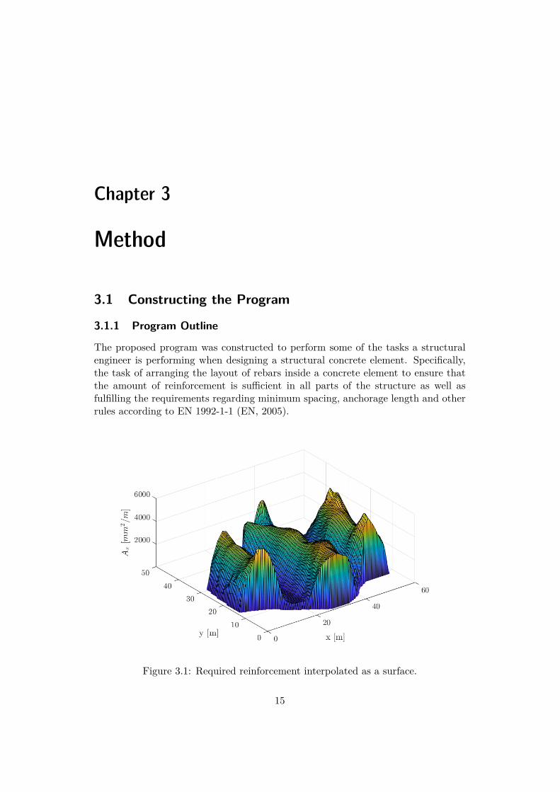
The proposed program was constructed to perform some of the tasks a structuralengineer is performing when designing a structural concrete element. Specifically,the task of arranging the layout of rebars inside a concrete element to ensure thatthe amount of reinforcement is su�cient in all parts of the structure as well asfulfilling the requirements regarding minimum spacing, anchorage length and otherrules according to EN 1992-1-1 (EN, 2005).
Figure 3.1: Required reinforcement interpolated as a surface.
15

16 CHAPTER 3. METHOD
Data for the required reinforcement is used as input to the program to arrangethe reinforcement layout. An example of how the required reinforcement data isscattered along the nodes of the structure is shown in Figure 3.1. The output dataof the program is a proposal of reinforcement layout, as well as the total amount ofreinforcement and the number of di�erent rebar used.
Similar to the design procedure used in a traditional design, the program isdivided into three main modules. The flowchart can be seen in Figure 3.2.
The first module was designed to choose a combination of rebar dimensions andcentre-to-centre (c.t.c) distances, as well as how the levels of reinforcement are ar-ranged. These variables are chosen in a manner that limits the excess reinforcementused while not using too many di�erent combinations, which would yield a com-plicated design. The second module is using the di�erent reinforcement levels tocalculate the required anchorage length depending on the results from module 1.
Finally, the third module was constructed to adjust the groups of reinforcementin order to find a satisfactory trade-o� between the number of di�erent lengths ofrebar elements and the excess reinforcement volume from adjusting these lengths.

3.1. CONSTRUCTING THE PROGRAM 17
Start
Initialize model
Requiredreinforcement
dataUser settings
Call Module 1? User rebar inputModule 1:
Optimizeselection of rebar
Module 2:
Adjust data forreinforcement
anchorage
Find placement ofminimum amountof reinforcement
Call Module 3?
Module 3:
Find trade-o�solution between
reinforcementmaterial usage
and buildability
Calculate totalamount of
reinforcementand number
of rebar types
Save resultsStop
yesno
yes
no
Figure 3.2: Program flowchart
3.1.2 Module 1
The first level of optimization was designed to search for a feasible and e�ectivecombination of reinforcement diameter „, c.t.c. distance c and the number of rein-forcement levels n
l
to use.The possible reinforcement diameters are determined by the available stock sizes
but might also be limited by the preferences of the contractor or which diametersthat are used elsewhere in the structure. Defining which levels to use is dependingon how many di�erent groups of rebar that is considered feasible for a buildable
18 CHAPTER 3. METHOD
solution. The c.t.c. distances are normally selected from a discrete range of dis-tances due to buildability reasons. According to the reasoning in Section 2.5 andthe discrete range of the variables that are to be optimized, the module is using agenetic algorithm optimization.
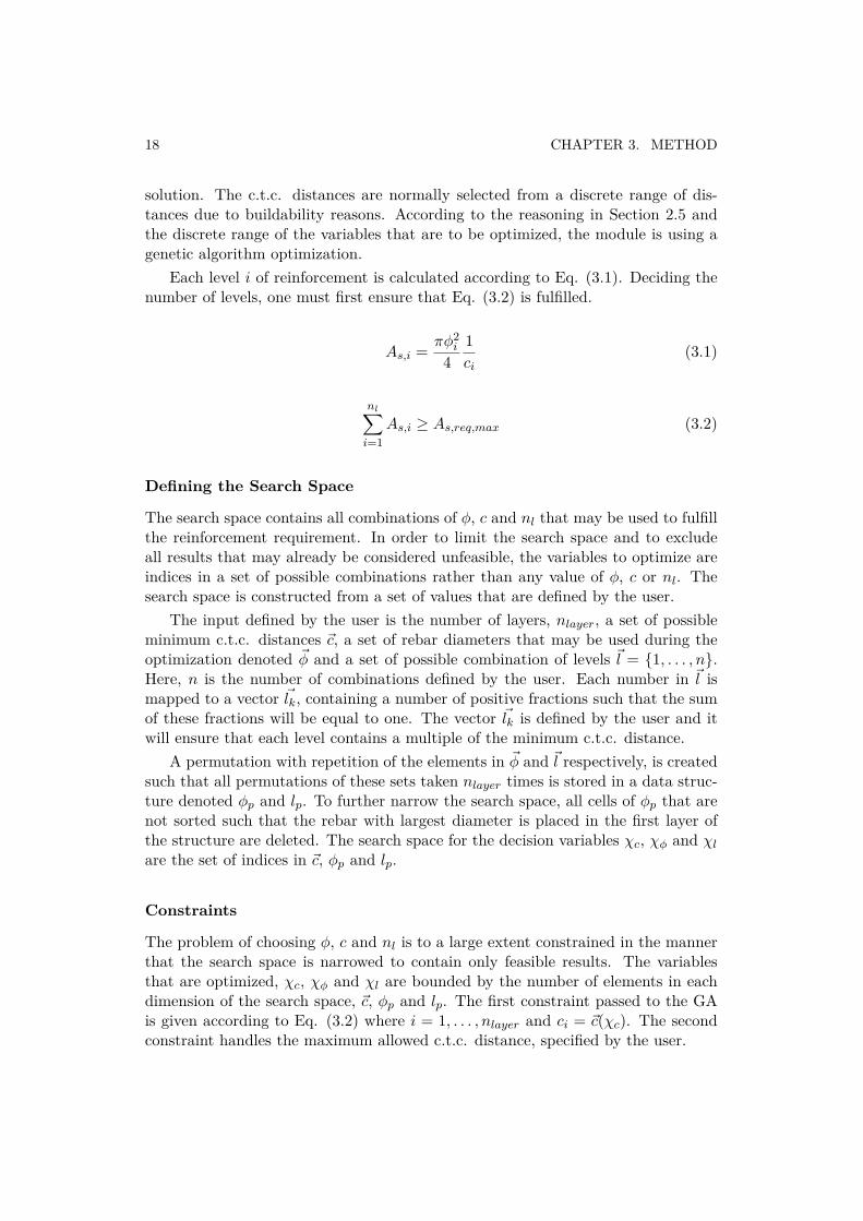
Each level i of reinforcement is calculated according to Eq. (3.1). Deciding thenumber of levels, one must first ensure that Eq. (3.2) is fulfilled.
A
s,i
= fi„
2i
41c
i
(3.1)
n
lÿ
i=1A
s,i
Ø A
s,req,max
(3.2)
Defining the Search Space
The search space contains all combinations of „, c and n
l
that may be used to fulfillthe reinforcement requirement. In order to limit the search space and to excludeall results that may already be considered unfeasible, the variables to optimize areindices in a set of possible combinations rather than any value of „, c or n
l
. Thesearch space is constructed from a set of values that are defined by the user.
The input defined by the user is the number of layers, n
layer
, a set of possibleminimum c.t.c. distances c̨, a set of rebar diameters that may be used during theoptimization denoted ˛
„ and a set of possible combination of levels ˛
l = {1, . . . , n}.Here, n is the number of combinations defined by the user. Each number in ˛
l ismapped to a vector ˛
l
k
, containing a number of positive fractions such that the sumof these fractions will be equal to one. The vector ˛
l
k
is defined by the user and itwill ensure that each level contains a multiple of the minimum c.t.c. distance.
A permutation with repetition of the elements in ˛
„ and ˛
l respectively, is createdsuch that all permutations of these sets taken n
layer
times is stored in a data struc-ture denoted „
p
and l
p
. To further narrow the search space, all cells of „
p
that arenot sorted such that the rebar with largest diameter is placed in the first layer ofthe structure are deleted. The search space for the decision variables ‰
c
, ‰
„
and ‰
l
are the set of indices in c̨, „
p
and l
p
.
Constraints
The problem of choosing „, c and n
l
is to a large extent constrained in the mannerthat the search space is narrowed to contain only feasible results. The variablesthat are optimized, ‰
c
, ‰
„
and ‰
l
are bounded by the number of elements in eachdimension of the search space, c̨, „
p
and l
p
. The first constraint passed to the GAis given according to Eq. (3.2) where i = 1, . . . , n
layer
and c
i
= c̨(‰c
). The secondconstraint handles the maximum allowed c.t.c. distance, specified by the user.
3.1. CONSTRUCTING THE PROGRAM 19
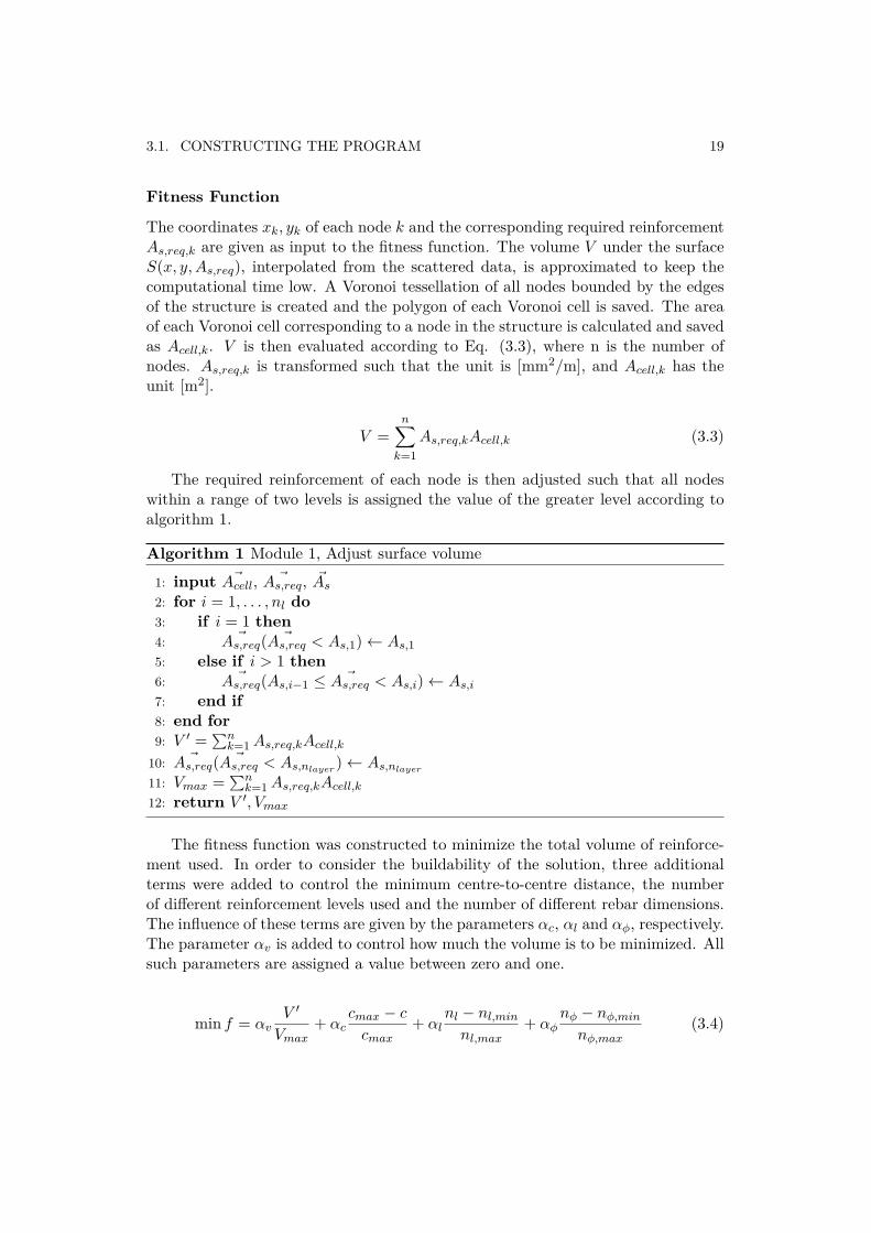
Fitness Function
The coordinates x
k
, y
k
of each node k and the corresponding required reinforcementA
s,req,k
are given as input to the fitness function. The volume V under the surfaceS(x, y, A
s,req
), interpolated from the scattered data, is approximated to keep thecomputational time low. A Voronoi tessellation of all nodes bounded by the edgesof the structure is created and the polygon of each Voronoi cell is saved. The areaof each Voronoi cell corresponding to a node in the structure is calculated and savedas A
cell,k
. V is then evaluated according to Eq. (3.3), where n is the number ofnodes. A
s,req,k
is transformed such that the unit is [mm2/m], and A
cell,k
has theunit [m2].
V =nÿ
k=1A
s,req,k
A
cell,k
(3.3)
The required reinforcement of each node is then adjusted such that all nodeswithin a range of two levels is assigned the value of the greater level according toalgorithm 1.
Algorithm 1 Module 1, Adjust surface volume1: input
˛
A
cell
, ˛
A
s,req
, ˛
A
s
2: for i = 1, . . . , n
l
do
3: if i = 1 then
4: ˛
A
s,req
( ˛
A
s,req
< A
s,1) Ω A
s,15: else if i > 1 then
6: ˛
A
s,req
(As,i≠1 Æ ˛
A
s,req
< A
s,i
) Ω A
s,i
7: end if
8: end for
9: V
Õ =q
n
k=1 A
s,req,k
A
cell,k
10: ˛
A
s,req
( ˛
A
s,req
< A
s,n
layer
) Ω A
s,n
layer
11: V
max
=q
n
k=1 A
s,req,k
A
cell,k
12: return V
Õ, V
max
The fitness function was constructed to minimize the total volume of reinforce-ment used. In order to consider the buildability of the solution, three additionalterms were added to control the minimum centre-to-centre distance, the numberof di�erent reinforcement levels used and the number of di�erent rebar dimensions.The influence of these terms are given by the parameters –
c
, –
l
and –
„
, respectively.The parameter –
v
is added to control how much the volume is to be minimized. Allsuch parameters are assigned a value between zero and one.
min f = –
v
V
Õ
V
max
+ –
c
c
max
≠ c
c
max
+ –
l
n
l
≠ n
l,min
n
l,max
+ –
„
n
„
≠ n
„,min
n
„,max
(3.4)
20 CHAPTER 3. METHOD
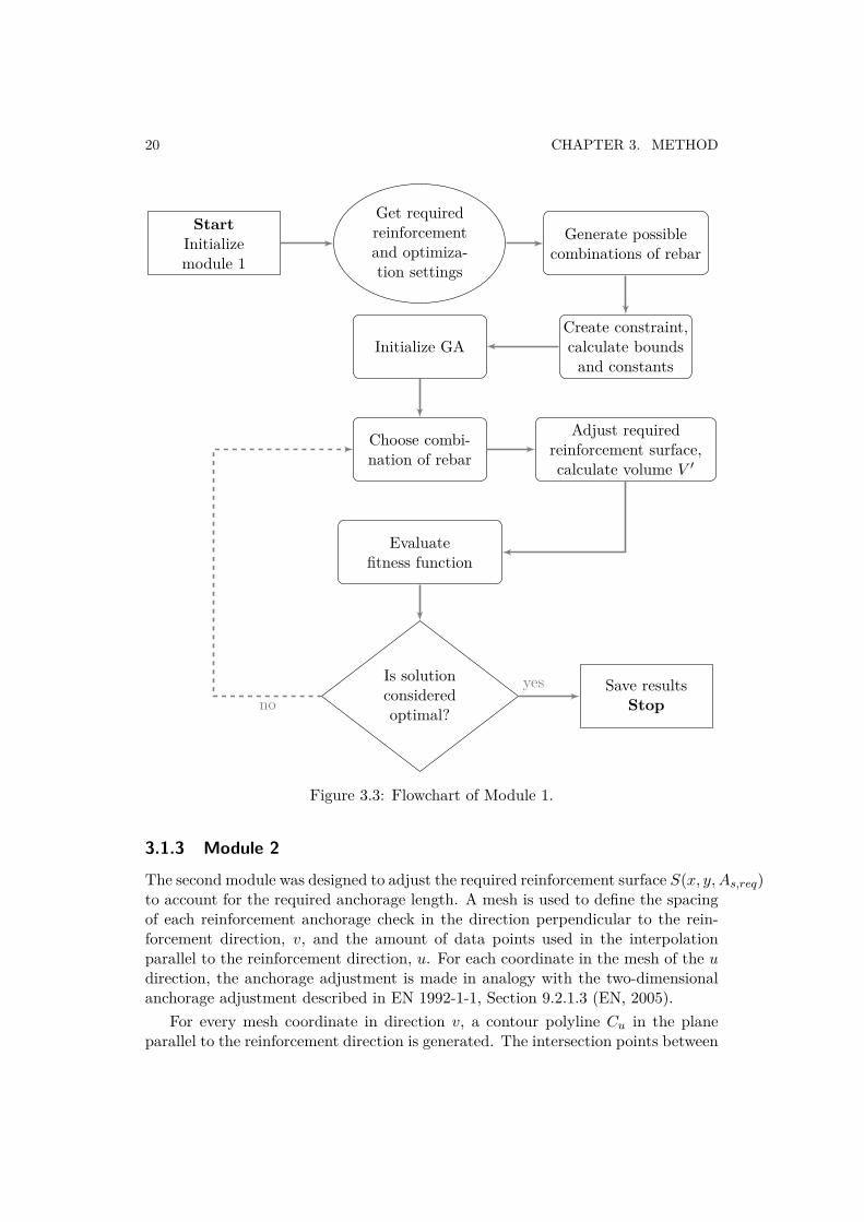
Start
Initializemodule 1
Get requiredreinforcementand optimiza-tion settings
Generate possiblecombinations of rebar
Create constraint,calculate bounds
and constantsInitialize GA
Choose combi-nation of rebar
Adjust requiredreinforcement surface,calculate volume V
Õ
Evaluatefitness function
Is solutionconsideredoptimal?
Save resultsStop
noyes
Figure 3.3: Flowchart of Module 1.
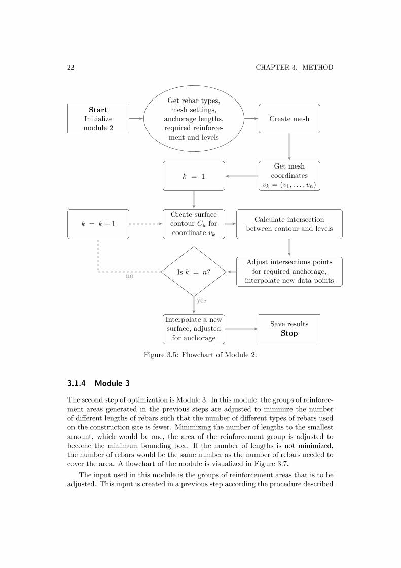
3.1.3 Module 2
The second module was designed to adjust the required reinforcement surface S(x, y, A
s,req
)to account for the required anchorage length. A mesh is used to define the spacingof each reinforcement anchorage check in the direction perpendicular to the rein-forcement direction, v, and the amount of data points used in the interpolationparallel to the reinforcement direction, u. For each coordinate in the mesh of the u
direction, the anchorage adjustment is made in analogy with the two-dimensionalanchorage adjustment described in EN 1992-1-1, Section 9.2.1.3 (EN, 2005).
For every mesh coordinate in direction v, a contour polyline C
u
in the planeparallel to the reinforcement direction is generated. The intersection points between
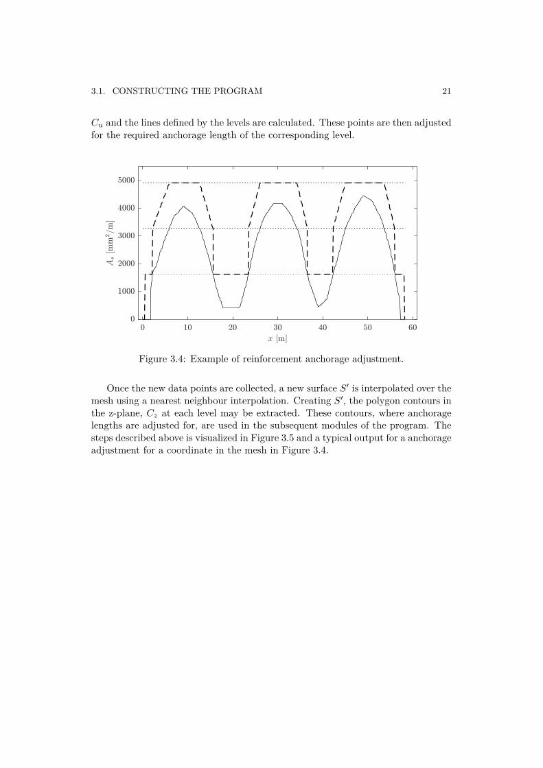
3.1. CONSTRUCTING THE PROGRAM 21
C
u
and the lines defined by the levels are calculated. These points are then adjustedfor the required anchorage length of the corresponding level.
Figure 3.4: Example of reinforcement anchorage adjustment.
Once the new data points are collected, a new surface S
Õ is interpolated over themesh using a nearest neighbour interpolation. Creating S
Õ, the polygon contours inthe z-plane, C
z
at each level may be extracted. These contours, where anchoragelengths are adjusted for, are used in the subsequent modules of the program. Thesteps described above is visualized in Figure 3.5 and a typical output for a anchorageadjustment for a coordinate in the mesh in Figure 3.4.
22 CHAPTER 3. METHOD
Start
Initializemodule 2
Get rebar types,mesh settings,
anchorage lengths,required reinforce-
ment and levels
Create mesh
Get meshcoordinates
v
k
= (v1, . . . , v
n
)k = 1
Create surfacecontour C
u
forcoordinate v
k
Calculate intersectionbetween contour and levels
Adjust intersections pointsfor required anchorage,
interpolate new data pointsIs k = n?
k = k + 1
Interpolate a newsurface, adjusted
for anchorage
Save resultsStop
no
yes
Figure 3.5: Flowchart of Module 2.
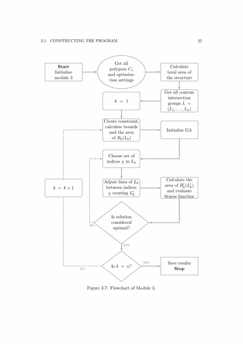
3.1.4 Module 3
The second step of optimization is Module 3. In this module, the groups of reinforce-ment areas generated in the previous steps are adjusted to minimize the numberof di�erent lengths of rebars such that the number of di�erent types of rebars usedon the construction site is fewer. Minimizing the number of lengths to the smallestamount, which would be one, the area of the reinforcement group is adjusted tobecome the minimum bounding box. If the number of lengths is not minimized,the number of rebars would be the same number as the number of rebars needed tocover the area. A flowchart of the module is visualized in Figure 3.7.
The input used in this module is the groups of reinforcement areas that is to beadjusted. This input is created in a previous step according the procedure described
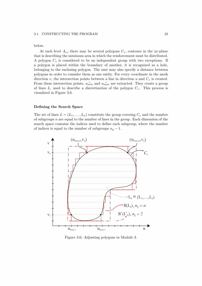
3.1. CONSTRUCTING THE PROGRAM 23
below.At each level A
s,i
there may be several polygons C
z
, contours in the xy-planethat is describing the minimum area in which the reinforcement must be distributed.A polygon C
z
is considered to be an independent group with two exceptions. Ifa polygon is placed within the boundary of another, it is recognized as a hole,belonging to the enclosing polygon. The user may also specify a distance betweenpolygons in order to consider them as one entity. For every coordinate in the meshdirection v, the intersection points between a line in direction u and C
z
is created.From these intersection points, ˛u
min
and ˛u
max
are extracted. They create a groupof lines L, used to describe a discretization of the polygon C
z
. This process isvisualized in Figure 3.6.
Defining the Search Space
The set of lines L = (L1, . . . , L
n
) constitute the group covering C
z
and the numberof subgroups n are equal to the number of lines in the group. Each dimension of thesearch space contains the indices used to define each subgroup, where the numberof indices is equal to the number of subgroups n
g
≠ 1.
uumin,1 umax,1
vn
v1
(umin,n,vn) (umax,n,vn)
Lk = (L1,...,Ln)
v
B’(L’k), ng = 2
B(Lk), ng = n
Cz
Figure 3.6: Adjusting polygons in Module 3.
24 CHAPTER 3. METHOD
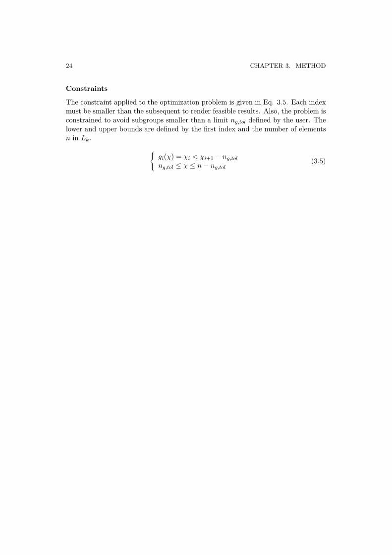
Constraints
The constraint applied to the optimization problem is given in Eq. 3.5. Each indexmust be smaller than the subsequent to render feasible results. Also, the problem isconstrained to avoid subgroups smaller than a limit n
g,tol
defined by the user. Thelower and upper bounds are defined by the first index and the number of elementsn in L
k
.I
g
i
(‰) = ‰
i
< ‰
i+1 ≠ n
g,tol
n
g,tol
Æ ‰ Æ n ≠ n
g,tol
(3.5)
3.1. CONSTRUCTING THE PROGRAM 25
Start
Initializemodule 3
Get allpolygons C
z
and optimiza-tion settings
Calculatetotal area ofthe structure
Get all contourintersectiongroups L =(L1, . . . , L
n
)k = 1
Create constraint,calculate bounds
and the areaof B
k
(Lk
)Initialize GA
Choose set ofindices ‰ in L
k
Adjust lines of L
k
between indices‰ creating L
Õk
Calculate thearea of B
Õk
(LÕk
)and evaluate
fitness function
Is solutionconsideredoptimal?
k = k + 1
Is k = n?Save results
Stop
no
no
yes
yes
Figure 3.7: Flowchart of Module 3.
26 CHAPTER 3. METHOD
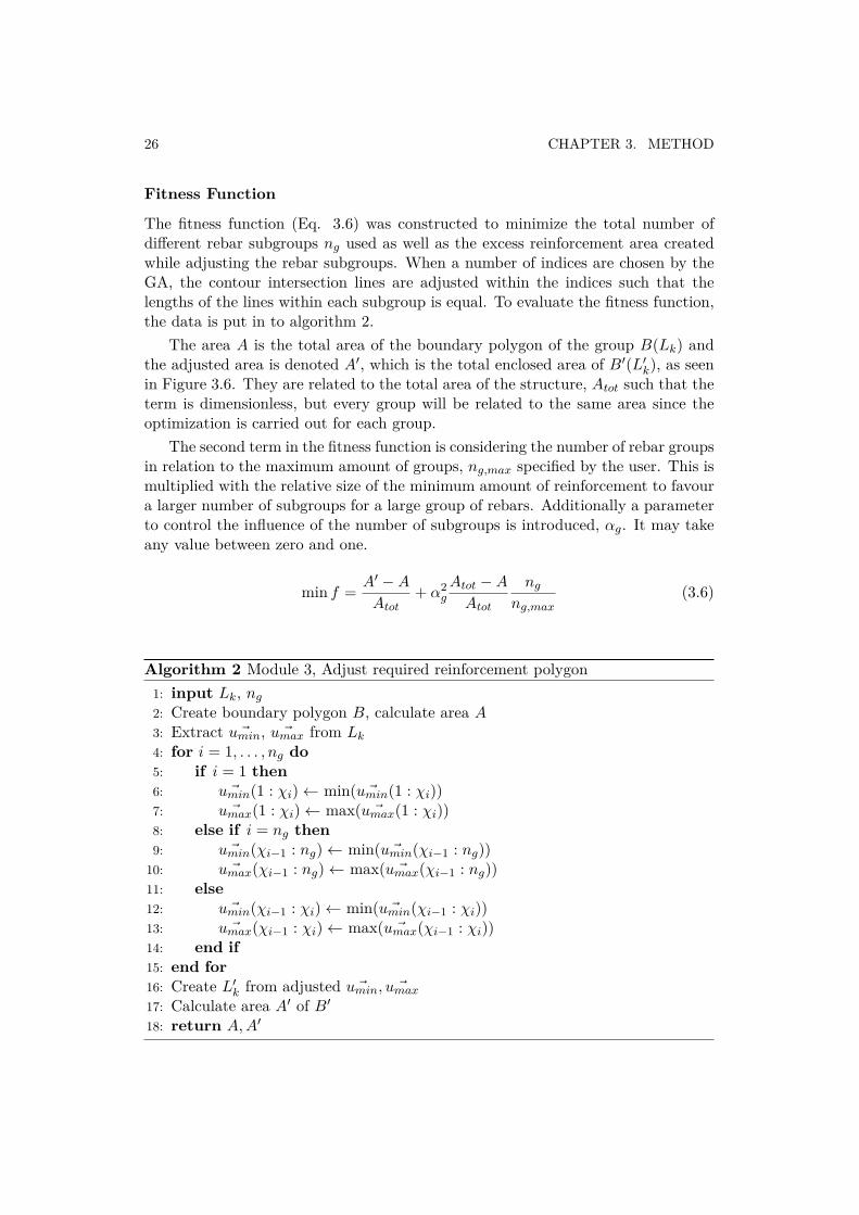
Fitness Function
The fitness function (Eq. 3.6) was constructed to minimize the total number ofdi�erent rebar subgroups n
g
used as well as the excess reinforcement area createdwhile adjusting the rebar subgroups. When a number of indices are chosen by theGA, the contour intersection lines are adjusted within the indices such that thelengths of the lines within each subgroup is equal. To evaluate the fitness function,the data is put in to algorithm 2.
The area A is the total area of the boundary polygon of the group B(Lk
) andthe adjusted area is denoted A
Õ, which is the total enclosed area of B
Õ(LÕk
), as seenin Figure 3.6. They are related to the total area of the structure, A
tot
such that theterm is dimensionless, but every group will be related to the same area since theoptimization is carried out for each group.
The second term in the fitness function is considering the number of rebar groupsin relation to the maximum amount of groups, n
g,max
specified by the user. This ismultiplied with the relative size of the minimum amount of reinforcement to favoura larger number of subgroups for a large group of rebars. Additionally a parameterto control the influence of the number of subgroups is introduced, –
g
. It may takeany value between zero and one.
min f = A
Õ ≠ A
A
tot
+ –
2g
A
tot
≠ A
A
tot
n
g
n
g,max
(3.6)
Algorithm 2 Module 3, Adjust required reinforcement polygon1: input L
k
, n
g
2: Create boundary polygon B, calculate area A
3: Extract ˛u
min
, ˛u
max
from L
k
4: for i = 1, . . . , n
g
do
5: if i = 1 then
6: ˛u
min
(1 : ‰
i
) Ω min( ˛u
min
(1 : ‰
i
))7: ˛u
max
(1 : ‰
i
) Ω max( ˛u
max
(1 : ‰
i
))8: else if i = n
g
then
9: ˛u
min
(‰i≠1 : n
g
) Ω min( ˛u
min
(‰i≠1 : n
g
))10: ˛u
max
(‰i≠1 : n
g
) Ω max( ˛u
max
(‰i≠1 : n
g
))11: else
12: ˛u
min
(‰i≠1 : ‰
i
) Ω min( ˛u
min
(‰i≠1 : ‰
i
))13: ˛u
max
(‰i≠1 : ‰
i
) Ω max( ˛u
max
(‰i≠1 : ‰
i
))14: end if
15: end for
16: Create L
Õk
from adjusted ˛u
min
, ˛u
max
17: Calculate area A
Õ of B
Õ
18: return A, A
Õ
3.2. MODEL VALIDATION 27
3.2 Model Validation
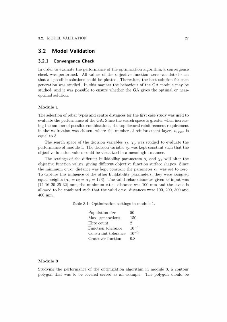
3.2.1 Convergence CheckIn order to evaluate the performance of the optimization algorithm, a convergencecheck was performed. All values of the objective function were calculated suchthat all possible solutions could be plotted. Thereafter, the best solution for eachgeneration was studied. In this manner the behaviour of the GA module may bestudied, and it was possible to ensure whether the GA gives the optimal or near-optimal solution.
Module 1
The selection of rebar types and centre distances for the first case study was used toevaluate the performance of the GA. Since the search space is greater when increas-ing the number of possible combinations, the top flexural reinforcement requirementin the x-direction was chosen, where the number of reinforcement layers n
layer
isequal to 3.
The search space of the decision variables ‰
l
, ‰
„
was studied to evaluate theperformance of module 1. The decision variable ‰
c
was kept constant such that theobjective function values could be visualized in a meaningful manner.
The settings of the di�erent buildability parameters –
l
and ‰
„
will alter theobjective function values, giving di�erent objective function surface shapes. Sincethe minimum c.t.c. distance was kept constant the parameter –
c
was set to zero.To capture this influence of the other buildability parameters, they were assignedequal weights (–
v
= –
l
= –
„
= 1/3). The valid rebar diametes given as input was[12 16 20 25 32] mm, the minimum c.t.c. distance was 100 mm and the levels isallowed to be combined such that the valid c.t.c. distances were 100, 200, 300 and400 mm.
Table 3.1: Optimization settings in module 1.
Population size 50Max. generations 150Elite count 2Function tolerance 10≠6
Constraint tolerance 10≠6
Crossover fraction 0.8
Module 3
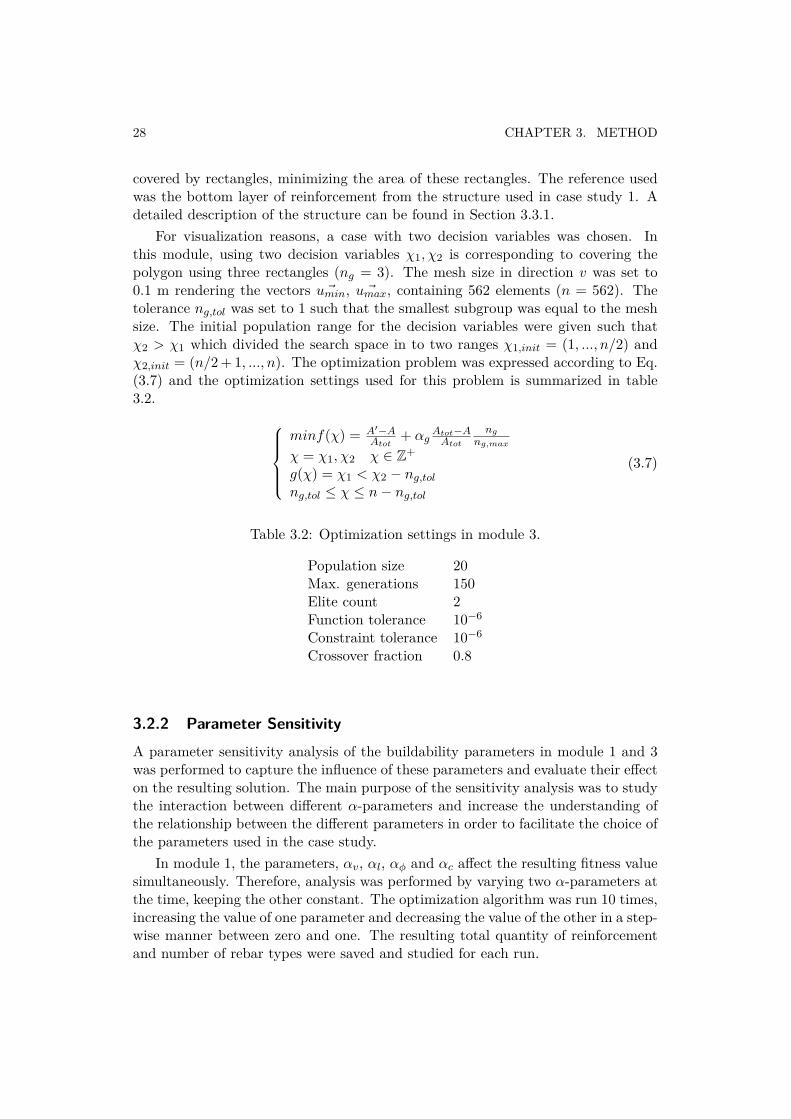
Studying the performance of the optimization algorithm in module 3, a contourpolygon that was to be covered served as an example. The polygon should be
28 CHAPTER 3. METHOD
covered by rectangles, minimizing the area of these rectangles. The reference usedwas the bottom layer of reinforcement from the structure used in case study 1. Adetailed description of the structure can be found in Section 3.3.1.
For visualization reasons, a case with two decision variables was chosen. Inthis module, using two decision variables ‰1, ‰2 is corresponding to covering thepolygon using three rectangles (n
g
= 3). The mesh size in direction v was set to0.1 m rendering the vectors ˛u
min
, ˛u
max
, containing 562 elements (n = 562). Thetolerance n
g,tol
was set to 1 such that the smallest subgroup was equal to the meshsize. The initial population range for the decision variables were given such that‰2 > ‰1 which divided the search space in to two ranges ‰1,init
= (1, ..., n/2) and‰2,init
= (n/2 + 1, ..., n). The optimization problem was expressed according to Eq.(3.7) and the optimization settings used for this problem is summarized in table3.2.
Y___]
___[
minf(‰) = A
Õ≠A
A
tot
+ –
g
A
tot
≠A
A
tot
n
g
n
g,max
‰ = ‰1, ‰2 ‰ œ Z+
g(‰) = ‰1 < ‰2 ≠ n
g,tol
n
g,tol
Æ ‰ Æ n ≠ n
g,tol
(3.7)
Table 3.2: Optimization settings in module 3.
Population size 20Max. generations 150Elite count 2Function tolerance 10≠6
Constraint tolerance 10≠6
Crossover fraction 0.8
3.2.2 Parameter SensitivityA parameter sensitivity analysis of the buildability parameters in module 1 and 3was performed to capture the influence of these parameters and evaluate their e�ecton the resulting solution. The main purpose of the sensitivity analysis was to studythe interaction between di�erent –-parameters and increase the understanding ofthe relationship between the di�erent parameters in order to facilitate the choice ofthe parameters used in the case study.
In module 1, the parameters, –
v
, –
l
, –
„
and –
c
a�ect the resulting fitness valuesimultaneously. Therefore, analysis was performed by varying two –-parameters atthe time, keeping the other constant. The optimization algorithm was run 10 times,increasing the value of one parameter and decreasing the value of the other in a step-wise manner between zero and one. The resulting total quantity of reinforcementand number of rebar types were saved and studied for each run.
3.3. CASE STUDY 29
To study the –
g
parameter in module 3, the optimization algorithm was run ina similar manner as for module 1, varying –
g
between zero and one and keeping the–-parameters in module 1 constant.
3.3 Case StudyTwo case studies were performed by analysing the results from the program andcomparing them to previously designed reinforced concrete structures. The objec-tive for performing the two case studies was to validate the optimization algorithmwith regard to buildability as well as its ability of performing a task similar toan engineer. The case study was carried out considering top and bottom flexuralreinforcement in two directions, which rendered four di�erent cases for each casestudy. Two-dimensional Cad drawings of the chosen structures, including specifi-cations of type, placement and distribution of reinforcing bars, provided basis forhand calculations of amount of required reinforcement and number of reinforcementbars.
The case study was performed in two steps where the first step involved deter-mining suitable values for the parameters in module 1 and 3 which take buildabilityinto account, here called –-parameters. The parameter –
g
in module 3, which con-trol the influence of the number of subgroups, was set to a value based on the resultsfrom the parameter sensitivity analysis in Section 3.2.2. To assign values to the –-parameters in module 1, the optimization algorithm was run multiple times for eachof the four cases with di�erent combinations of parameters, see Appendix A.1 andB.1. Each combination of parameters generated a solution which was evaluatedbased on buildability, total amount of reinforcement and number of di�erent typesof reinforcement bars. The assessment of buildability was carried out by evaluatinghow well the generated solution fulfilled the following buildability criterias:
• The dimension/centre distance ratio of rebars is su�ciently large.
• Few reinforcement levels are used rather than many whenever possible.
• Large rebar dimensions are used rather than small whenever possible.
• Centre distances of top flexural reinforcement are equal to or a multiple ofbottom flexural reinforcement c.t.c. distance.
• Rebars are distributed in few larger regions rather than many small regions.
Comparing the best results of each combination of –-parameters, a combinationof parameters was chosen which fulfilled the above mentioned criteria’s.
Following the first step of assigning values to the –-parameters, the second stepof the case study was performed by running the optimization algorithm for each ofthe four cases. The results from the algorithm were then compared with the resultsof the hand calculations and evaluated based on buildability aspects, similarity tosolution produced by an engineer and total quantity of reinforcement.
30 CHAPTER 3. METHOD
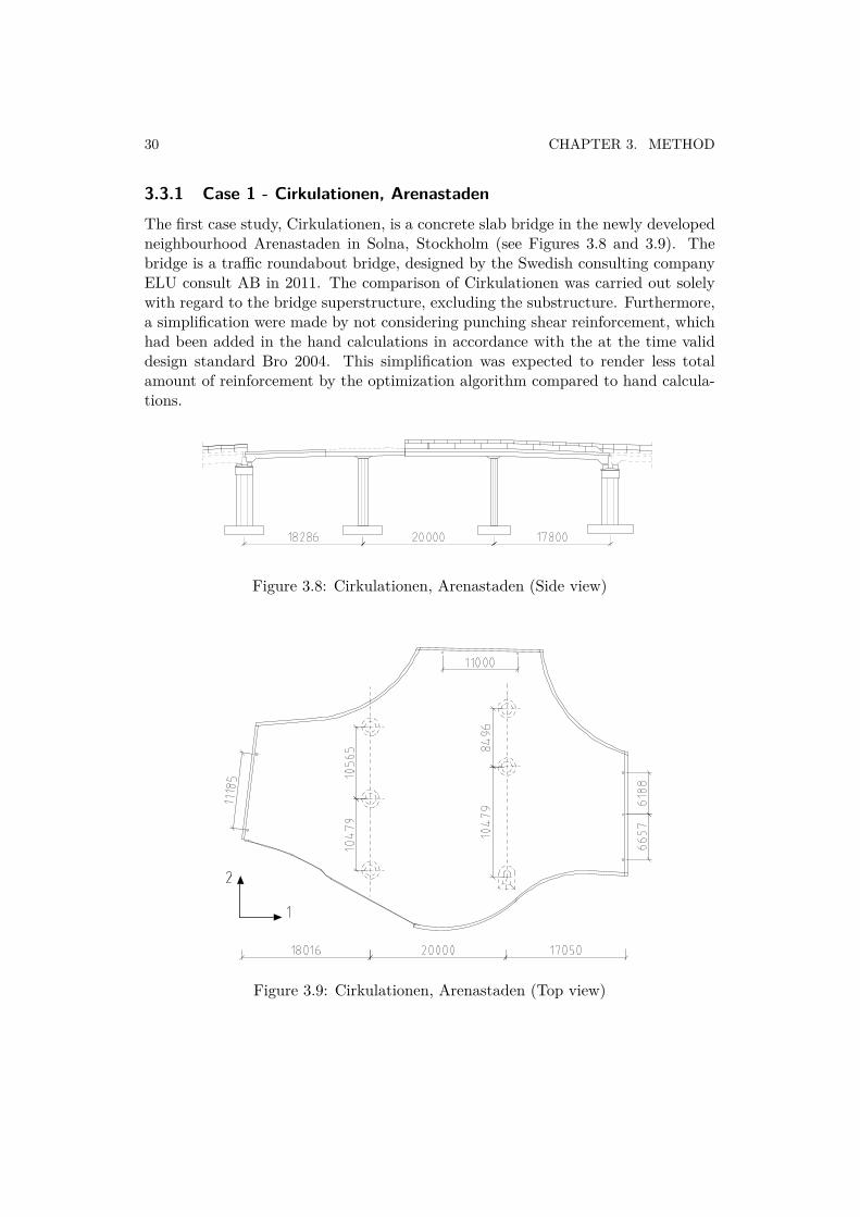
3.3.1 Case 1 - Cirkulationen, ArenastadenThe first case study, Cirkulationen, is a concrete slab bridge in the newly developedneighbourhood Arenastaden in Solna, Stockholm (see Figures 3.8 and 3.9). Thebridge is a tra�c roundabout bridge, designed by the Swedish consulting companyELU consult AB in 2011. The comparison of Cirkulationen was carried out solelywith regard to the bridge superstructure, excluding the substructure. Furthermore,a simplification were made by not considering punching shear reinforcement, whichhad been added in the hand calculations in accordance with the at the time validdesign standard Bro 2004. This simplification was expected to render less totalamount of reinforcement by the optimization algorithm compared to hand calcula-tions.
Figure 3.8: Cirkulationen, Arenastaden (Side view)
Figure 3.9: Cirkulationen, Arenastaden (Top view)

3.3. CASE STUDY 31
Table 3.3 show design assumptions and data used in the case study of Cirkula-tionen.
Table 3.3: Design assumptions and data
Total amount of concrete [m3] 1407No of layers (top flexural reinforcement) [pcs] 3No of layers (bottom flexural reinforcement) [pcs] 2Maximum no of subregions [pcs] 4Length [m] 56.1Thickness [m] 0.8
3.3.2 Case 2 - Slussen
The second case study is a concrete slab for a new canal sluice in Slussen, Stockholm.The slab is part of a larger sluice construction which is currently being designed bythe Swedish consulting company ELU consult AB, see Figures 3.10 and 3.11. Sincethe sluice construction is transported by sea, from the dock where it is being built tothe construction site in Slussen, extra reinforcement had been added to support theconstruction during transportation. A simplification was made in the optimizationalgorithm not considering this extra reinforcement and therefore it was expectedthat the total amount of reinforcement, calculated by the optimization algorithm,was to be less than hand calculations. Furthermore, only the red hatched area ofthe structure in Figure 3.11 was considered in the case study.
Figure 3.10: Slussen (Right-hand side of construction)

32 CHAPTER 3. METHOD
Figure 3.11: Slussen (Top view)
Table 3.4 show design assumptions and data used in the comparative study ofSlussen.
Table 3.4: Design assumptions and data
Total amount of concrete [m3] 1552No of layers [pcs] 2Maximum no of subregions [pcs] 4Length [m] 156Width [m] 24Thickness [m] 0.8
Chapter 4
Results
4.1 Model Validation
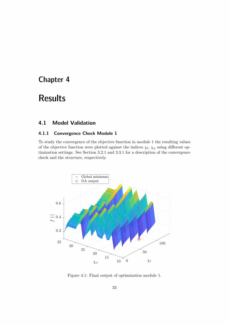
4.1.1 Convergence Check Module 1
To study the convergence of the objective function in module 1 the resulting valuesof the objective function were plotted against the indices ‰
l
, ‰
„
using di�erent op-timization settings. See Section 3.2.1 and 3.3.1 for a description of the convergencecheck and the structure, respectively.
Figure 4.1: Final output of optimization module 1.
33
34 CHAPTER 4. RESULTS
0.15
0.2
0.25
0.3
0.35
0.4
0.45
0.5
0.55
0.6
Figure 4.2: Initial population and best result per generation.
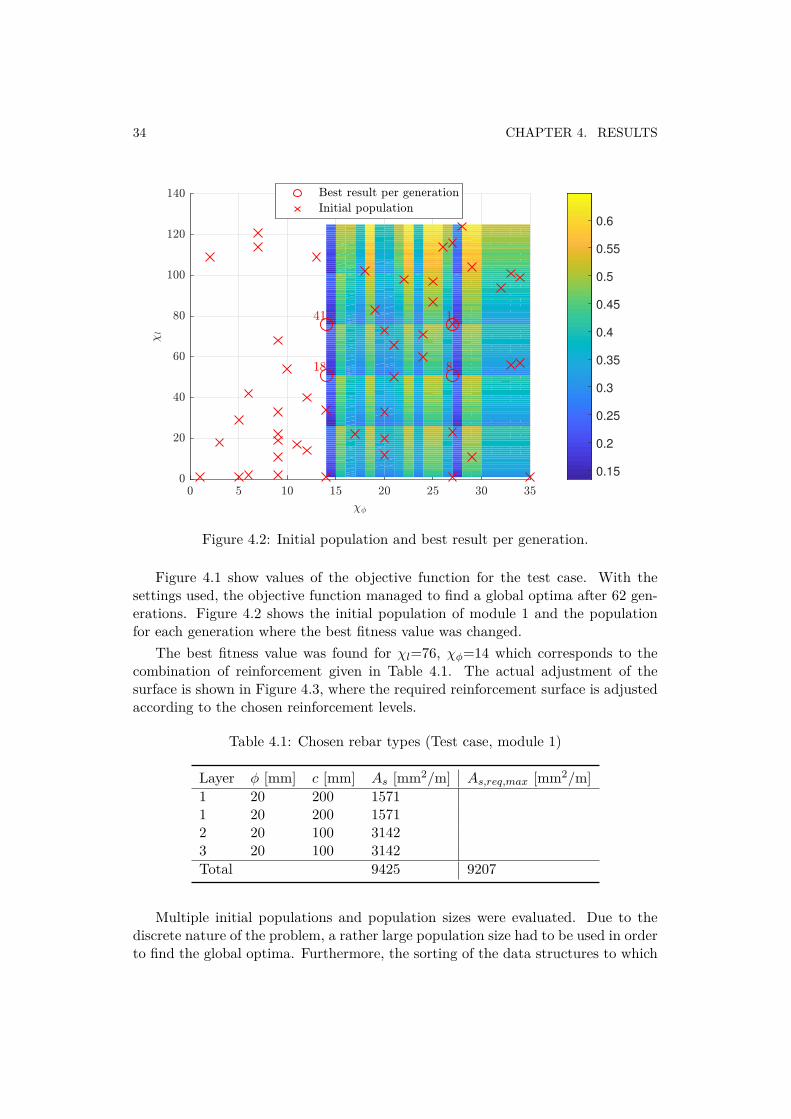
Figure 4.1 show values of the objective function for the test case. With thesettings used, the objective function managed to find a global optima after 62 gen-erations. Figure 4.2 shows the initial population of module 1 and the populationfor each generation where the best fitness value was changed.
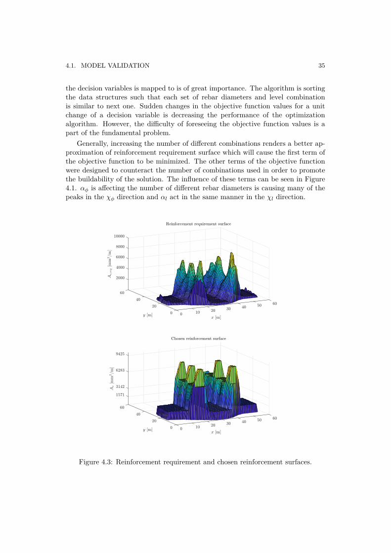
The best fitness value was found for ‰
l
=76, ‰
„
=14 which corresponds to thecombination of reinforcement given in Table 4.1. The actual adjustment of thesurface is shown in Figure 4.3, where the required reinforcement surface is adjustedaccording to the chosen reinforcement levels.
Table 4.1: Chosen rebar types (Test case, module 1)
Layer „ [mm] c [mm] A
s
[mm2/m] A
s,req,max
[mm2/m]1 20 200 15711 20 200 15712 20 100 31423 20 100 3142Total 9425 9207
Multiple initial populations and population sizes were evaluated. Due to thediscrete nature of the problem, a rather large population size had to be used in orderto find the global optima. Furthermore, the sorting of the data structures to which
4.1. MODEL VALIDATION 35
the decision variables is mapped to is of great importance. The algorithm is sortingthe data structures such that each set of rebar diameters and level combinationis similar to next one. Sudden changes in the objective function values for a unitchange of a decision variable is decreasing the performance of the optimizationalgorithm. However, the di�culty of foreseeing the objective function values is apart of the fundamental problem.
Generally, increasing the number of di�erent combinations renders a better ap-proximation of reinforcement requirement surface which will cause the first term ofthe objective function to be minimized. The other terms of the objective functionwere designed to counteract the number of combinations used in order to promotethe buildability of the solution. The influence of these terms can be seen in Figure4.1. –
„
is a�ecting the number of di�erent rebar diameters is causing many of thepeaks in the ‰
„
direction and –
l
act in the same manner in the ‰
l
direction.
Figure 4.3: Reinforcement requirement and chosen reinforcement surfaces.
36 CHAPTER 4. RESULTS
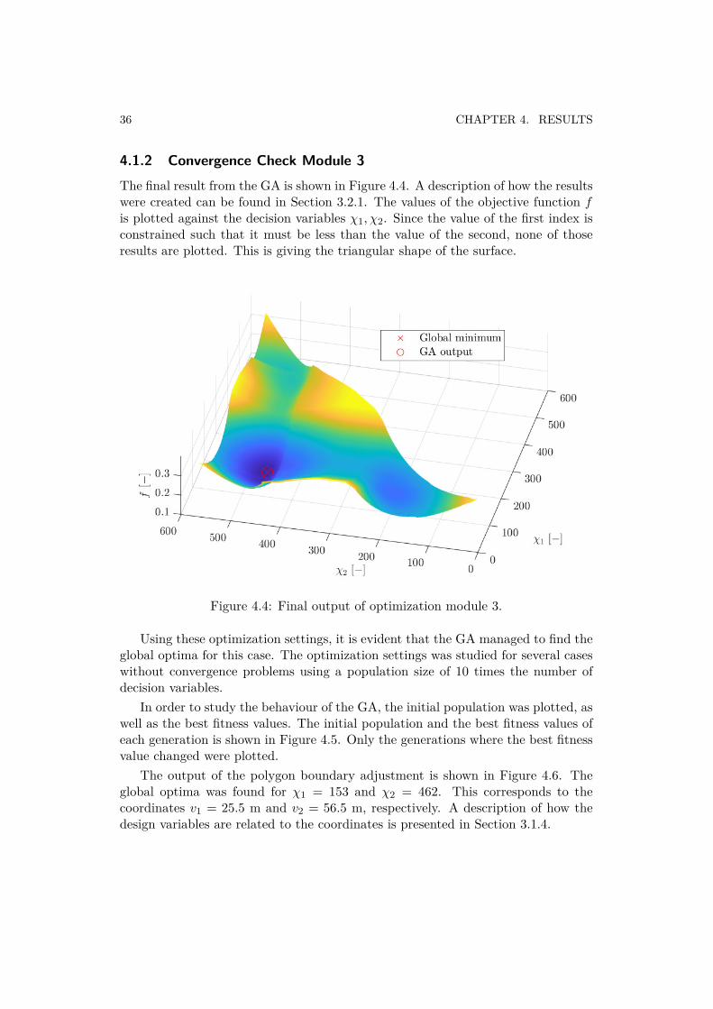
4.1.2 Convergence Check Module 3The final result from the GA is shown in Figure 4.4. A description of how the resultswere created can be found in Section 3.2.1. The values of the objective function f
is plotted against the decision variables ‰1, ‰2. Since the value of the first index isconstrained such that it must be less than the value of the second, none of thoseresults are plotted. This is giving the triangular shape of the surface.
Figure 4.4: Final output of optimization module 3.
Using these optimization settings, it is evident that the GA managed to find theglobal optima for this case. The optimization settings was studied for several caseswithout convergence problems using a population size of 10 times the number ofdecision variables.
In order to study the behaviour of the GA, the initial population was plotted, aswell as the best fitness values. The initial population and the best fitness values ofeach generation is shown in Figure 4.5. Only the generations where the best fitnessvalue changed were plotted.
The output of the polygon boundary adjustment is shown in Figure 4.6. Theglobal optima was found for ‰1 = 153 and ‰2 = 462. This corresponds to thecoordinates v1 = 25.5 m and v2 = 56.5 m, respectively. A description of how thedesign variables are related to the coordinates is presented in Section 3.1.4.

4.1. MODEL VALIDATION 37
Figure 4.5: Initial population and best fitness value per generation.
Figure 4.6: Polygon boundary adjustment.
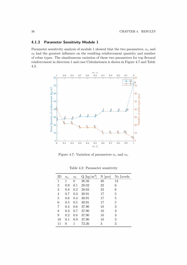
38 CHAPTER 4. RESULTS
4.1.3 Parameter Sensitivity Module 1
Parameter sensitivity analysis of module 1 showed that the two parameters, –
v
and–
l
had the greatest influence on the resulting reinforcement quantity and numberof rebar types. The simultaneous variation of these two parameters for top flexuralreinforcement in direction 1 and case Cirkulationen is shown in Figure 4.7 and Table4.2.
Figure 4.7: Variation of parameters –
v
and –
l
.
Table 4.2: Parameter sensitivity
ID –
v
–
l
Q [kg/m3] N [pcs] No Levels1 1 0 26.56 40 122 0.9 0.1 28.02 22 63 0.8 0.2 28.02 22 64 0.7 0.3 30.91 17 55 0.6 0.4 30.91 17 56 0.5 0.5 30.91 17 57 0.4 0.6 37.90 10 38 0.3 0.7 37.90 10 39 0.2 0.8 37.90 10 310 0.1 0.9 37.90 10 311 0 1 72.26 3 3
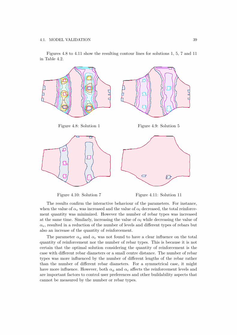
4.1. MODEL VALIDATION 39
Figures 4.8 to 4.11 show the resulting contour lines for solutions 1, 5, 7 and 11in Table 4.2.
Figure 4.8: Solution 1 Figure 4.9: Solution 5
Figure 4.10: Solution 7 Figure 4.11: Solution 11
The results confirm the interactive behaviour of the parameters. For instance,when the value of –
v
was increased and the value of –
l
decreased, the total reinforce-ment quantity was minimized. However the number of rebar types was increasedat the same time. Similarly, increasing the value of –
l
while decreasing the value of–
v
, resulted in a reduction of the number of levels and di�erent types of rebars butalso an increase of the quantity of reinforcement.
The parameter –
„
and –
c
was not found to have a clear influence on the totalquantity of reinforcement nor the number of rebar types. This is because it is notcertain that the optimal solution considering the quantity of reinforcement is thecase with di�erent rebar diameters or a small centre distance. The number of rebartypes was more influenced by the number of di�erent lengths of the rebar ratherthan the number of di�erent rebar diameters. For a symmetrical case, it mighthave more influence. However, both –
„
and –
c
a�ects the reinforcement levels andare important factors to control user preferences and other buildability aspects thatcannot be measured by the number or rebar types.

40 CHAPTER 4. RESULTS
4.1.4 Parameter Sensitivity Module 3
Figure 4.12 show parameter sensitivity analysis of –
g
for bottom flexural reinforce-ment in direction 1 for Cirkulationen. The settings used for this case was a maximumnumber of 10 rebar subgroups, a rebar dimension of 20 mm, a centre distance of200 mm and two reinforcement levels per layer, giving four reinforcement levels.
Figure 4.12: Variation of parameters –
g
Varying the parameter –
g
between 0 and 1 showed that the number of rebartypes decreased rapidly compared to the increase in quantity and that the largestdecrease was obtained for a –
g
-values between 0 and 0.5, see Figure 4.12. Tominimize the number of rebars in a layout a minimum value of 0.6 for –
g
is suggested.Figures 4.13 to 4.16 show solutions 1, 3, 6 and 11 in Figure 4.12.
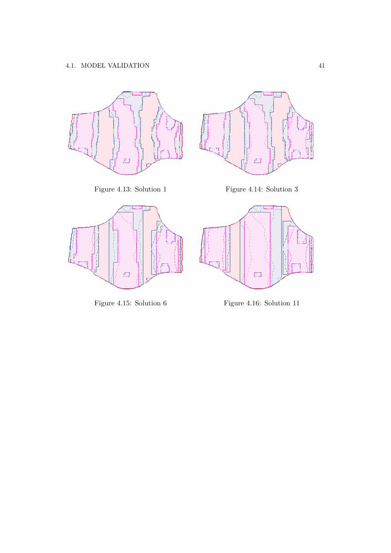
4.1. MODEL VALIDATION 41
Figure 4.13: Solution 1 Figure 4.14: Solution 3
Figure 4.15: Solution 6 Figure 4.16: Solution 11
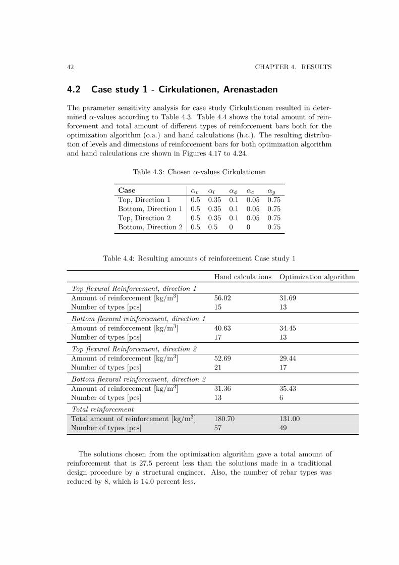
42 CHAPTER 4. RESULTS
4.2 Case study 1 - Cirkulationen, Arenastaden
The parameter sensitivity analysis for case study Cirkulationen resulted in deter-mined –-values according to Table 4.3. Table 4.4 shows the total amount of rein-forcement and total amount of di�erent types of reinforcement bars both for theoptimization algorithm (o.a.) and hand calculations (h.c.). The resulting distribu-tion of levels and dimensions of reinforcement bars for both optimization algorithmand hand calculations are shown in Figures 4.17 to 4.24.
Table 4.3: Chosen –-values Cirkulationen
Case –
v
–
l
–
„
–
c
–
g
Top, Direction 1 0.5 0.35 0.1 0.05 0.75Bottom, Direction 1 0.5 0.35 0.1 0.05 0.75Top, Direction 2 0.5 0.35 0.1 0.05 0.75Bottom, Direction 2 0.5 0.5 0 0 0.75
Table 4.4: Resulting amounts of reinforcement Case study 1
Hand calculations Optimization algorithmTop flexural Reinforcement, direction 1Amount of reinforcement [kg/m3] 56.02 31.69Number of types [pcs] 15 13Bottom flexural reinforcement, direction 1Amount of reinforcement [kg/m3] 40.63 34.45Number of types [pcs] 17 13Top flexural Reinforcement, direction 2Amount of reinforcement [kg/m3] 52.69 29.44Number of types [pcs] 21 17Bottom flexural reinforcement, direction 2Amount of reinforcement [kg/m3] 31.36 35.43Number of types [pcs] 13 6Total reinforcementTotal amount of reinforcement [kg/m3] 180.70 131.00Number of types [pcs] 57 49
The solutions chosen from the optimization algorithm gave a total amount ofreinforcement that is 27.5 percent less than the solutions made in a traditionaldesign procedure by a structural engineer. Also, the number of rebar types wasreduced by 8, which is 14.0 percent less.
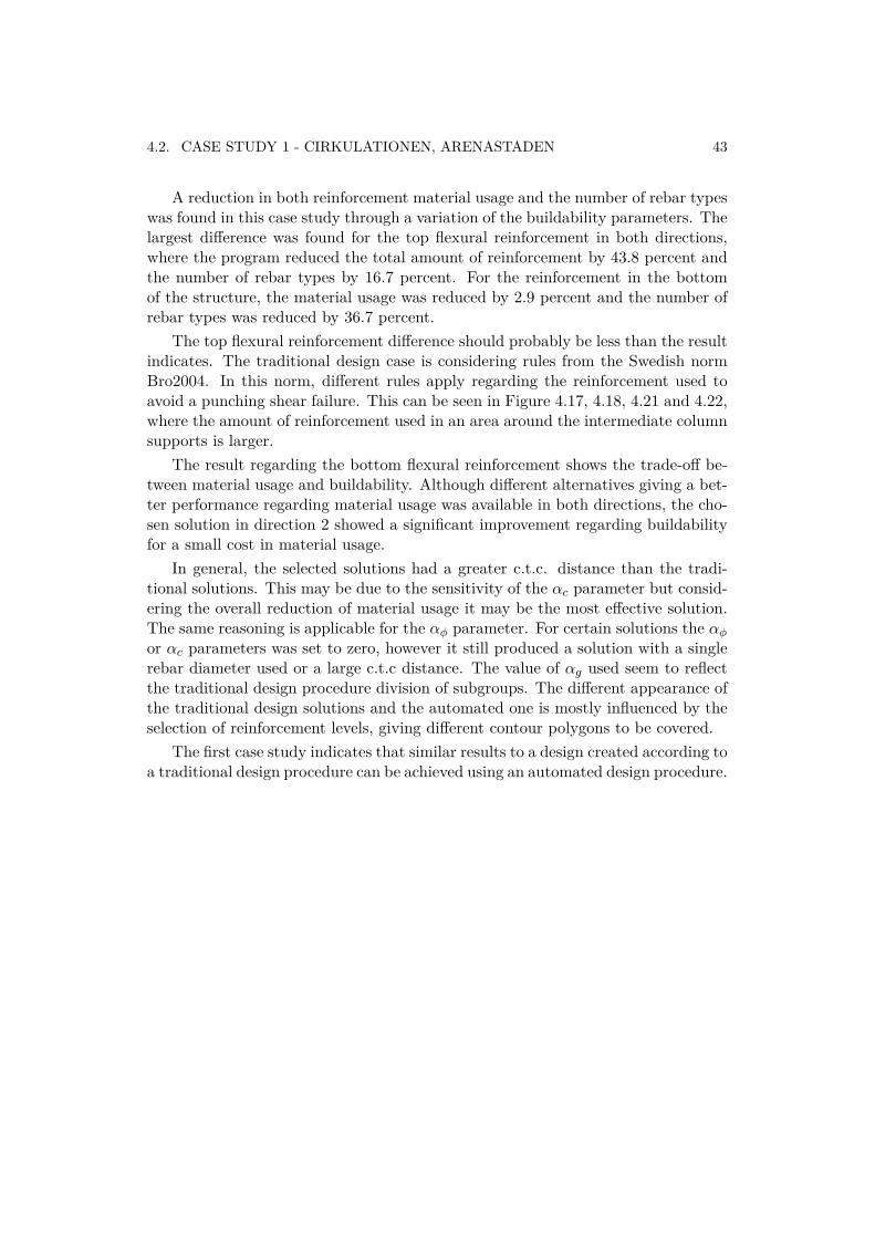
4.2. CASE STUDY 1 - CIRKULATIONEN, ARENASTADEN 43
A reduction in both reinforcement material usage and the number of rebar typeswas found in this case study through a variation of the buildability parameters. Thelargest di�erence was found for the top flexural reinforcement in both directions,where the program reduced the total amount of reinforcement by 43.8 percent andthe number of rebar types by 16.7 percent. For the reinforcement in the bottomof the structure, the material usage was reduced by 2.9 percent and the number ofrebar types was reduced by 36.7 percent.
The top flexural reinforcement di�erence should probably be less than the resultindicates. The traditional design case is considering rules from the Swedish normBro2004. In this norm, di�erent rules apply regarding the reinforcement used toavoid a punching shear failure. This can be seen in Figure 4.17, 4.18, 4.21 and 4.22,where the amount of reinforcement used in an area around the intermediate columnsupports is larger.
The result regarding the bottom flexural reinforcement shows the trade-o� be-tween material usage and buildability. Although di�erent alternatives giving a bet-ter performance regarding material usage was available in both directions, the cho-sen solution in direction 2 showed a significant improvement regarding buildabilityfor a small cost in material usage.
In general, the selected solutions had a greater c.t.c. distance than the tradi-tional solutions. This may be due to the sensitivity of the –
c
parameter but consid-ering the overall reduction of material usage it may be the most e�ective solution.The same reasoning is applicable for the –
„
parameter. For certain solutions the –
„
or –
c
parameters was set to zero, however it still produced a solution with a singlerebar diameter used or a large c.t.c distance. The value of –
g
used seem to reflectthe traditional design procedure division of subgroups. The di�erent appearance ofthe traditional design solutions and the automated one is mostly influenced by theselection of reinforcement levels, giving di�erent contour polygons to be covered.
The first case study indicates that similar results to a design created according toa traditional design procedure can be achieved using an automated design procedure.
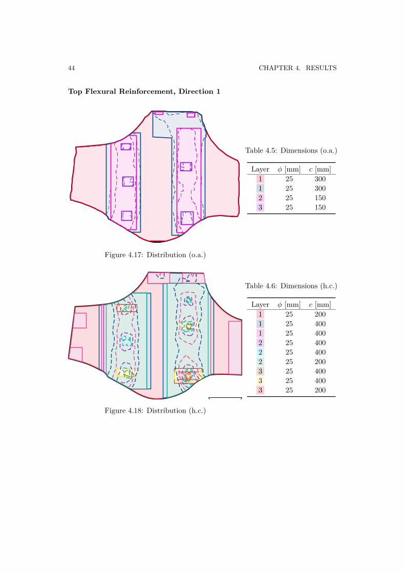
44 CHAPTER 4. RESULTS
Top Flexural Reinforcement, Direction 1
Figure 4.17: Distribution (o.a.)
Table 4.5: Dimensions (o.a.)
Layer „ [mm] c [mm]1 25 3001 25 3002 25 1503 25 150
Figure 4.18: Distribution (h.c.)
Table 4.6: Dimensions (h.c.)
Layer „ [mm] c [mm]1 25 2001 25 4001 25 4002 25 4002 25 4002 25 2003 25 4003 25 4003 25 200
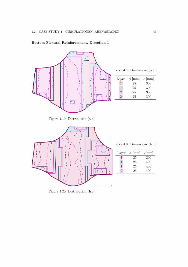
4.2. CASE STUDY 1 - CIRKULATIONEN, ARENASTADEN 45
Bottom Flexural Reinforcement, Direction 1
Figure 4.19: Distribution (o.a.)
Table 4.7: Dimensions (o.a.)
Layer „ [mm] c [mm]1 25 3001 25 3002 25 3002 25 300
Figure 4.20: Distribution (h.c.)
Table 4.8: Dimensions (h.c.)
Layer „ [mm] c[mm]1 25 2001 25 4001 25 4002 25 400
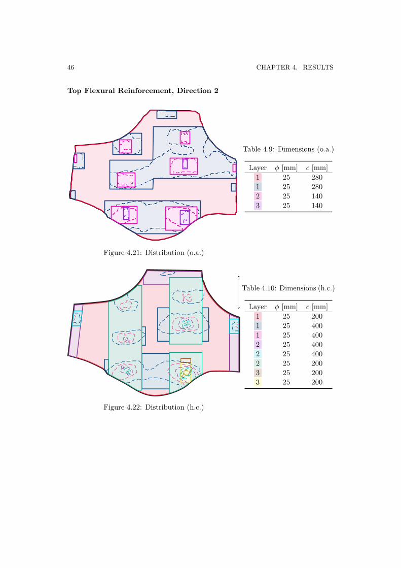
46 CHAPTER 4. RESULTS
Top Flexural Reinforcement, Direction 2
Figure 4.21: Distribution (o.a.)
Table 4.9: Dimensions (o.a.)
Layer „ [mm] c [mm]1 25 2801 25 2802 25 1403 25 140
Figure 4.22: Distribution (h.c.)
Table 4.10: Dimensions (h.c.)
Layer „ [mm] c [mm]1 25 2001 25 4001 25 4002 25 4002 25 4002 25 2003 25 2003 25 200

4.2. CASE STUDY 1 - CIRKULATIONEN, ARENASTADEN 47
Bottom Flexural Reinforcement, Direction 2
Figure 4.23: Distribution (o.a.)
Table 4.11: Dimensions (o.a.)
Layer „ [mm] c [mm]1 25 1402 25 140
Figure 4.24: Distribution (h.c.)
Table 4.12: Dimensions (h.c.)
Layer „ [mm] c [mm]1 25 2001 25 4001 25 4002 25 4002 25 400
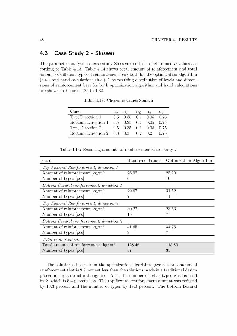
48 CHAPTER 4. RESULTS
4.3 Case Study 2 - SlussenThe parameter analysis for case study Slussen resulted in determined –-values ac-cording to Table 4.13. Table 4.14 shows total amount of reinforcement and totalamount of di�erent types of reinforcement bars both for the optimization algorithm(o.a.) and hand calculations (h.c.). The resulting distribution of levels and dimen-sions of reinforcement bars for both optimization algorithm and hand calculationsare shown in Figures 4.25 to 4.32.
Table 4.13: Chosen –-values Slussen
Case –
v
–
l
–
„
–
c
–
g
Top, Direction 1 0.5 0.35 0.1 0.05 0.75Bottom, Direction 1 0.5 0.35 0.1 0.05 0.75Top, Direction 2 0.5 0.35 0.1 0.05 0.75Bottom, Direction 2 0.3 0.3 0.2 0.2 0.75
Table 4.14: Resulting amounts of reinforcement Case study 2
Case Hand calculations Optimization AlgorithmTop Flexural Reinforcement, direction 1Amount of reinforcement [kg/m3] 26.92 25.90Number of types [pcs] 6 10Bottom flexural reinforcement, direction 1Amount of reinforcement [kg/m3] 29.67 31.52Number of types [pcs] 7 11Top Flexural Reinforcement, direction 2Amount of reinforcement [kg/m3] 30.22 23.63Number of types [pcs] 15 7Bottom flexural reinforcement, direction 2Amount of reinforcement [kg/m3] 41.65 34.75Number of types [pcs] 9 7Total reinforcementTotal amount of reinforcement [kg/m3] 128.46 115.80Number of types [pcs] 37 35
The solutions chosen from the optimization algorithm gave a total amount ofreinforcement that is 9.9 percent less than the solutions made in a traditional designprocedure by a structural engineer. Also, the number of rebar types was reducedby 2, which is 5.4 percent less. The top flexural reinforcement amount was reducedby 13.3 percent and the number of types by 19.0 percent. The bottom flexural
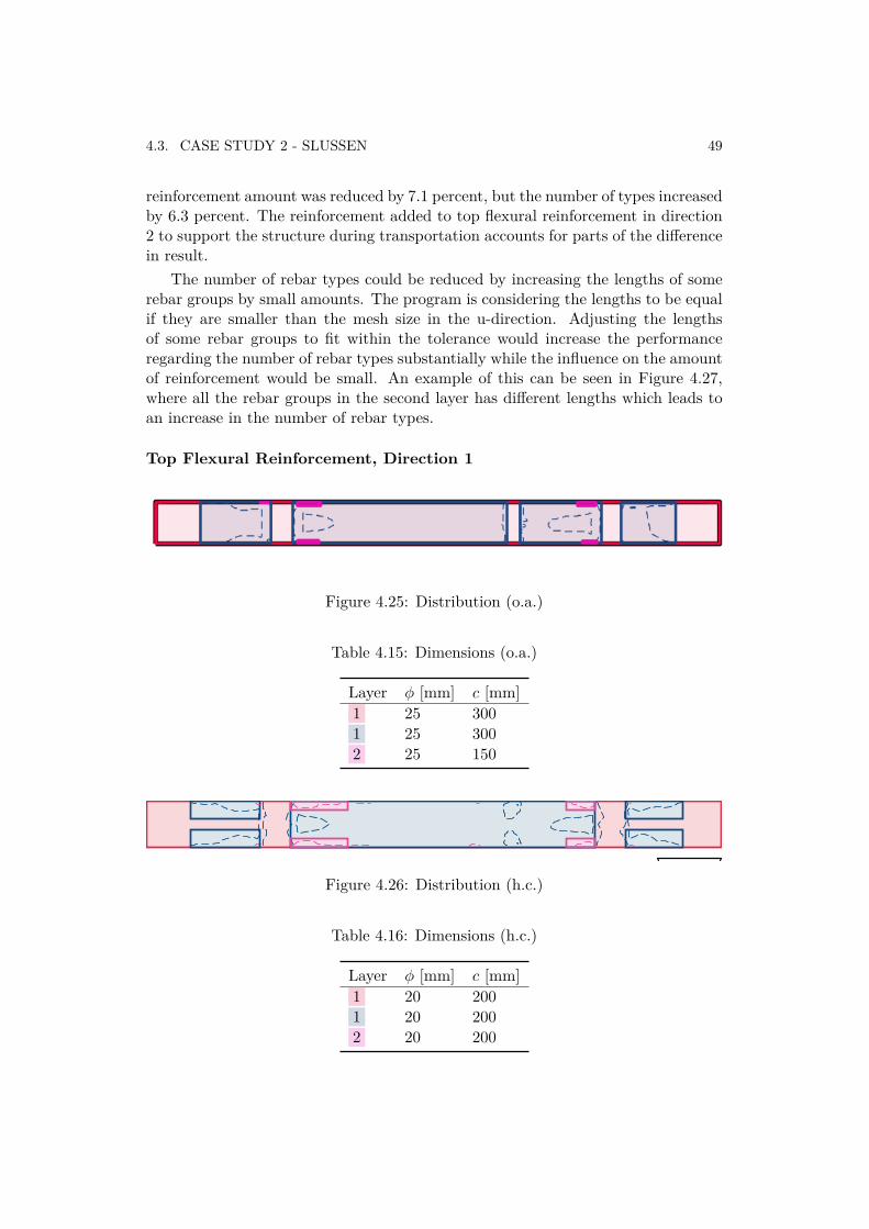
4.3. CASE STUDY 2 - SLUSSEN 49
reinforcement amount was reduced by 7.1 percent, but the number of types increasedby 6.3 percent. The reinforcement added to top flexural reinforcement in direction2 to support the structure during transportation accounts for parts of the di�erencein result.
The number of rebar types could be reduced by increasing the lengths of somerebar groups by small amounts. The program is considering the lengths to be equalif they are smaller than the mesh size in the u-direction. Adjusting the lengthsof some rebar groups to fit within the tolerance would increase the performanceregarding the number of rebar types substantially while the influence on the amountof reinforcement would be small. An example of this can be seen in Figure 4.27,where all the rebar groups in the second layer has di�erent lengths which leads toan increase in the number of rebar types.
Top Flexural Reinforcement, Direction 1
Figure 4.25: Distribution (o.a.)
Table 4.15: Dimensions (o.a.)
Layer „ [mm] c [mm]1 25 3001 25 3002 25 150
Figure 4.26: Distribution (h.c.)
Table 4.16: Dimensions (h.c.)
Layer „ [mm] c [mm]1 20 2001 20 2002 20 200
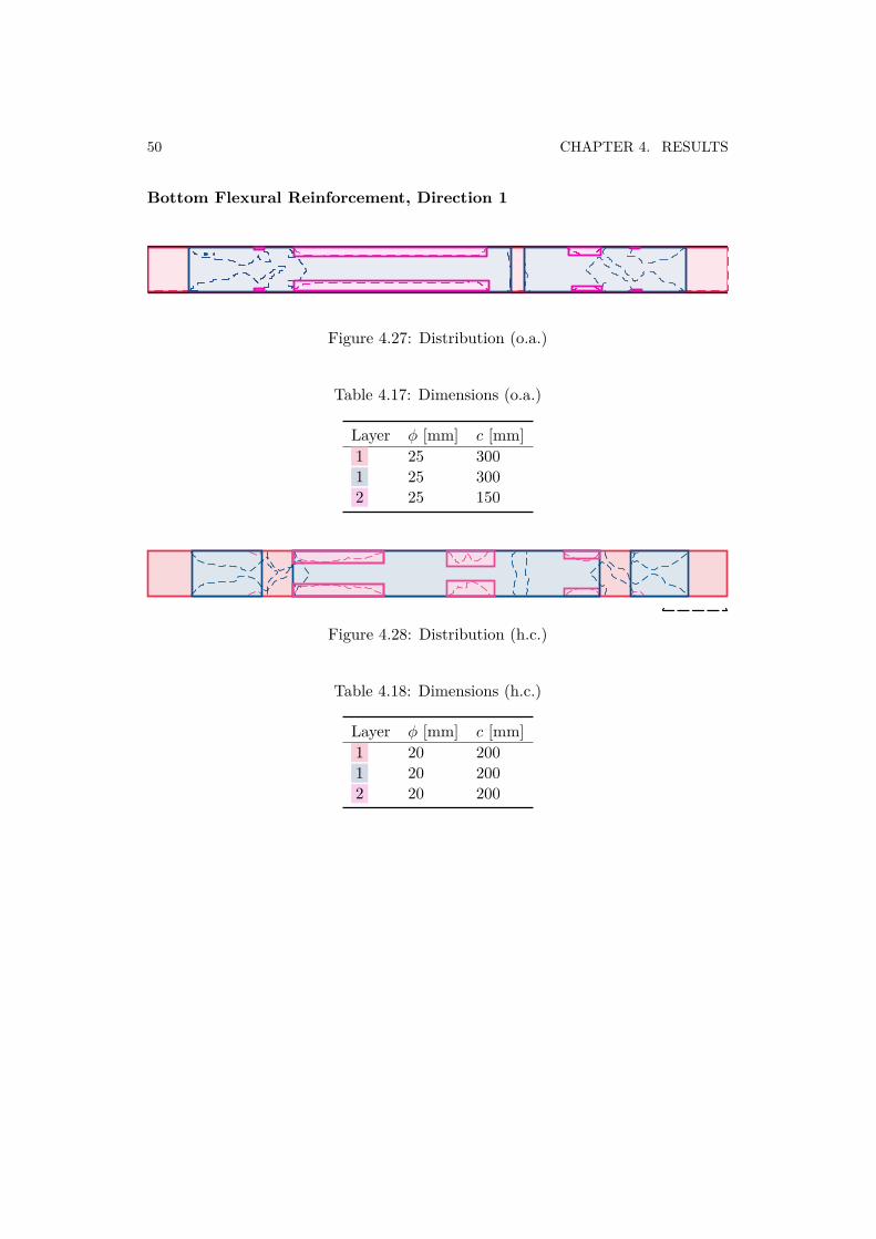
50 CHAPTER 4. RESULTS
Bottom Flexural Reinforcement, Direction 1
Figure 4.27: Distribution (o.a.)
Table 4.17: Dimensions (o.a.)
Layer „ [mm] c [mm]1 25 3001 25 3002 25 150
Figure 4.28: Distribution (h.c.)
Table 4.18: Dimensions (h.c.)
Layer „ [mm] c [mm]1 20 2001 20 2002 20 200
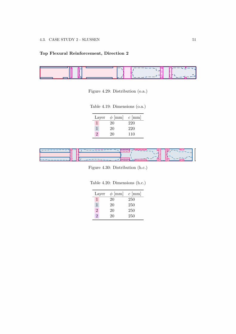
4.3. CASE STUDY 2 - SLUSSEN 51
Top Flexural Reinforcement, Direction 2
Figure 4.29: Distribution (o.a.)
Table 4.19: Dimensions (o.a.)
Layer „ [mm] c [mm]1 20 2201 20 2202 20 110
Figure 4.30: Distribution (h.c.)
Table 4.20: Dimensions (h.c.)
Layer „ [mm] c [mm]1 20 2501 20 2502 20 2502 20 250
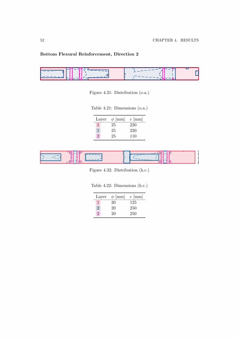
52 CHAPTER 4. RESULTS
Bottom Flexural Reinforcement, Direction 2
Figure 4.31: Distribution (o.a.)
Table 4.21: Dimensions (o.a.)
Layer „ [mm] c [mm]1 25 2201 25 2202 25 110
Figure 4.32: Distribution (h.c.)
Table 4.22: Dimensions (h.c.)
Layer „ [mm] c [mm]1 20 1252 20 2502 20 250
Chapter 5
Discussion and Conclusions
5.1 Discussion
In this thesis, a computer program has been developed to perform the process ofcreating a reinforcement design of a concrete structure. An approach to automatethis process was created by identifying the key aspects of the reinforcement layoutdesign according to previous literature as well as by examination of design drawings.
To find feasible solutions, an optimization algorithm was used. Due to the natureof the problem and the characteristics of the decision variables, a GA was selectedfor the ability of solving discrete optimization problems. The inability to guaranteean optimal solution to the problem using heuristic methods is not considered to becrucial since the best solution will be determined by many factors that are di�cultto quantify. Also, the computational time of using an exhaustive search method isconsidered impractical and would limit the usefulness of the program.
It is important to remember that the main idea is not to find a design that issupposed to be considered optimal for every case, rather a method to find a feasiblesolution according to the preferences of the user. Thus, keeping the computationaltime low, promoting the user-friendliness of the program and producing an optimalor near-optimal solution was considered more important than the guarantee of anoptimal solution.
To ensure that the optimization algorithms was returning an acceptable solution,a rather large population sizes had to be used. This is a drawback of optimizingdiscrete variables using a GA. Increasing the population size increases number ofcalculations at the cost of computational e�ort. To keep the computational timelow, the program is using approximations evaluating the objective functions and theproblem is divided in to two separate optimizations which might discard potentialdesign solutions.
An example of this is that the objective function of module 1 approximates thevolume under the surface and gives a penalty for the number of reinforcement levelsused. Increasing the number of levels was found to generally increase the number of
53
54 CHAPTER 5. DISCUSSION AND CONCLUSIONS
rebar types since there will be more polygons to cover in module 3. However, thisdepends on the shape of reinforcement requirement surface. Therefore, a solutionfrom module 1 that uses few reinforcement levels might be discarded since theobjective function is not evaluating the total amount of reinforcement of the finalsolution.
A part of the work that is traditionally being conducted during the design pro-cess is making decisions regarding spurious results from the FE-model. When au-tomating the design process, it is important to pre-process the data to account forthis before running the algorithm. Typical situations are singularities caused bypoint loads or geometric discontinuities.
The program developed only consider the spatial arrangement of the contourpolygons by a tolerance considering the distance between the polygons that allowsthe program to consider multiple polygons as a single entity. In the results fromthe case studies there are some solutions where a designer might cover the polygonsdi�erently. Di�erent rules of considering this could be implemented to improve thealgorithm.
Considering the buildability of the solutions, the objective functions was de-signed to capture some of the key features creating a feasible solution. Definingan objective function to fit a somewhat arbitrary goal that might di�er dependingon the project, the preferences of the contractor or the preferences of the engineeris a di�cult aspect. In the objective functions designed, each term was added todefine a cost associated with choosing a less buildable solution. The sizes of thesecosts will di�er depending on the input defined by the user. As an example, in theobjective function of module 1, the size of the term considering centre distances isdependent of the largest centre distance that is given as input. In a future study, itwould be interesting to redefine the objective functions to consider di�erent costs.
There are some di�erences regarding the prerequisites of the traditional designand the design created by the program in the case studies, particularly for the topflexural reinforcement for case study 1. This adds some uncertainty to the results,especially regarding the amount of reinforcement used. The ability of the programto create a feasible layout based on the contours can still be evaluated like the othersolutions.
One of the benefits of using an automated design process is that it is possible tosave time in the design phase. The time-saving renders a possibility to explore de-sign options that is di�cult to find using a traditional design procedure. An exampleof this is the parameter sensitivity analysis in Section 4.1.3 and 4.1.4. Visualizingthe trade-o� between buildability and material usage requires more design solutionsthan what would have been feasible to create without an automated design proce-dure. Likewise, adapting a set-based design method the concrete reinforcementdesign requires an e�ective technique to produce multiple designs.
Varying the parameters has shown some di�erences in the reinforcement layoutdesign. A large benefit of dividing the process in to modules that are performing
5.2. CONCLUSIONS 55
part of the task is the ability to control the process. It is possible to use this programas a tool to explore design options regarding rebar types and centre distances, but itmay also be used to calculate the required reinforcement anchorage length for everypoint in the structure if the designer wishes to only utilize part of the program.This possibility for interaction is important when automating a design process.
5.2 ConclusionsThe results from this study indicates that the reinforcement layout design proceduremay be subject to automation. According to the quantities that were selected asthe measure of the e�ectiveness and the buildability of the solution, the programmanaged to find designs that may be considered feasible. By the variation of thebuildability parameters, it was also shown that the consideration of buildability hasa direct impact on the reinforcement material usage.
5.3 Future ResearchAlthough the program managed to find designs that may be considered feasible, theprogram can be further improved in the future.
The heuristic nature of the problem encourages investigations of implementingan AI algorithm to analyse traditional designs and find ways of improving the in-corporation of the decision-making process of the designer. The incorporation ofdecision-making can also be further improved by an extended exploration of theobjective functions and the buildability parameters. It is recommended to furtherresearch the buildability parameters in this study, both quantitatively and qualita-tively. Qualitative studies may include performing interviews with contractors orother parties with knowledge of how consideration to buildability a�ects work onsite.
As of now, calculations performed for top and bottom flexural reinforcement arenot linked together. In order to improve buildability of the solutions the calcula-tions should be linked in such way that the centre distance of the bottom flexuralreinforcement being the same or a multiple of the top flexural reinforcement.
To expand the area of application of the program it is recommended that addi-tional types and geometries of reinforcement bars are incorporated into the program,for example bent bars. Additional rules in Eurocode should also be included intothe program, for example rules regarding overlapping bars and redistributions oversupports.
Module 3 could be further improved by implementation of di�erent ways ofcovering the contours of the required reinforcement, for example by allowing thesubareas to merge and separate.

Bibliography
Back, T., Fogel, D., and Michalewicz, Z. Evolutionary Computation 1. Basic Al-gorithms and Operators. PhD thesis, Institute of physics Publishing, Bristol andPhiladelphia, 2000.
BIM Alliance. Vad är bim?, 2018. URL http://www.bimalliance.se/vad-aer-
bim/.
Burke, E. and Kendall, G. Search Methodologies: Introductory Tutorials in Opti-mization and Decision Support Techniques. Springer, Boston, MA, 2014.
Concrete Reinforcing Steel Institute (CRSI), 2013. URL http://www.crsi.org/.
Construction Industry Institute (CII), 2018. URL https://www.construction-
institute.org/.
Construction industry research and information association (CIRIA), 2018. URLhttps://www.ciria.org/.
Dorigo, M. Optimization, Learning and Natural Algorithms, PhD thesis. PhD thesis,Politecnico di Milano, Italy, 1992.
EN 1992-1-1 Eurocode 2: Design of concrete structures - Part 1-1: General ruelsand rules for buildings, Brussels, 2005. EN, CEN.
Engstrom, D., Hyll, H., Fredsdotter, J., and Larsson, R. Armering i byggprocessen -e�ektivisering av informationshanteringen. NCC Construction Sverige AB, 2011.
Goldberg, D. Genetic Algorithms in search, Optimization, and Machine Learning".Addison-Wesley, 1989.
Holland, J. Adaptation in natural and artificial systems. The University of MichiganPress, 1975.
Holland, J. Genetic algorithms. Scientific American, 267:66–73, 1992.
Horn, A. Integrating Constructability into Conceptual Structural Design and Opti-mization. PhD thesis, Massachusetts Institute of Technology, 2015.
57

58 BIBLIOGRAPHY
Kennedy, J. and Eberhart, R. Particle swarm optimization. Proc. of IEEE Inter-national Conference on Neural Networks, pages 1942–1948, 1995.
Kirkpatrick, S., Gelatt, C., and Vecchi, M. Optimization by simulated annealing.Sience, New Series, 220:671–680, 1983.
Lam, P. T. I., Wong, F. W. H., and Chan, A. P. C. Contributions of designers toimproving buildability and constructability. PhD thesis, Department of Buildingand Real Estate, The Hong Kong Polytechnic University, Hong Kong, 2005.
Liker, J., Sobek II, D., Ward, A., and Christiano, J. Involving suppliers in productdevelopment in the united states; and japan: Evidence for set-based concurrentengineering. IEEE Transactions on Engineering Management, 43, 1996.
MathWorks. Matlab, 2018. URL https://se.mathworks.com/products/matlab.
html.
Mitchell, M. An Introduction to Genetic Algorithms. The MIT Press, 1999.
Pardalos, P. and Romeijn, H. Handbook of global optimization. Volume 2. SpringerScience and Business Media, 2002.
Parrish, K., Wong, J.-M., Tommelein, I., and Stojadinovic, B. Exploration of set-based design for reinforced concrete structures. University of California, Berkeley,2007.
Sandberg, M., Gerth, R., Lu, W., Jansson, G., Mukkavaara, J., and Olofsson, T.Design automation in construction: an overview. In 33rd CIB W78 Conference2016, Oct. 31st–Nov. 2nd 2016, Brisbane, Australia, 2016.
Simonsson, P. Buildability of Concrete Structures: Processes, Methods and Ma-terial. PhD thesis, Department of Civil, Environmental and Natural ResourcesEngineering, Lulea University of Technology, 2011.
Sobek II, D., Ward, A., and Liker, J. Toyota’s principles of set-based concurrentengineering. Sloan Management Review, 1999.
Tauriainen, M., Puttonen, J., and Saari, A. The assessment of constructability:BIM Cases. PhD thesis, Aalto University, School of Engineering, Department ofCivil and Structural Engineering, Espoo, Finland, 2015.
Templeman, B., A. Discrete optimum structural design. Computers and Structures,30:511–518, 1988.
Ward, A., Liker, J., Christiano, J., and Sobek II, D. The second toyota paradox:How delaying decisions can make better cars faster. Sloan Management Review,pages 43–61, 1995.

BIBLIOGRAPHY 59
Ward, A. and Seering, W. Quantitative Inference in a Mechanical Design "Com-plier". PhD thesis, Massachusetts Institute of Technology, 1989.
Yang, X.-S. and Deb, S. Engineering optimisation by cuckoo search. Int. J. Math-ematical Modelling and Numerical Optimisation, 1(4):330–343, 2010.


Appendix A
Case study 1 - Cirkulationen
A.1 Parameter Sensitivity Case 1A.1.1 Top Flexural Reinforcement, Direction 1Table A.1 shows results for –-parameter sensitivity analysis performed for top flex-ural reinforcement in direction 1. The chosen solution is highlighted in orange andthe solutions presented in the appendix is highlighted in grey.
Table A.1: Parameter sensitivity result
ID –
v
–
l
–
„
–
c
–
g
Q [kg/m3] N [pcs] Á
Q
[%] Á
N
[pcs]1 1 0 0 0 0.75 23.85 41 57 262 0 1 0 0 0.75 47.75 6 15 93 0.5 0.5 0 0 0.75 31.14 12 44 34 0.75 0.25 0 0 0.75 25.42 24 55 95 0.25 0.75 0 0 0.75 37.90 9 32 66 0 0.25 0.75 0 0.75 47.75 6 15 97 0 0.25 0 0.75 0.75 39.11 9 30 68 0.25 0.25 0.25 0.25 0.75 31.69 13 43 39 0.5 0.35 0.1 0.05 0.75 31.69 13 43 310 0.3 0.3 0.2 0.2 0.75 31.69 13 43 3
61

62 APPENDIX A. CASE STUDY 1 - CIRKULATIONEN
Solution ID 1
Figure A.1: Distribution
Table A.2: Dimensions
Layer „ [mm] c [mm]1 20 4001 20 4001 20 4001 20 4002 20 4002 20 4002 20 4002 20 4003 20 4003 20 4003 20 4003 20 400
Table A.3: Parameter sensitivity result
ID –
v
–
l
–
„
–
c
–
g
Q [kg/m3] N [pcs] Á
Q
[%] Á
N
[pcs]1 1 0 0 0 0.75 23.85 41 57 26
Solution ID 2
Figure A.2: Distribution
Table A.4: Dimensions
Layer „ [mm] c [mm]1 25 1002 20 100
Table A.5: Parameter sensitivity result
ID –
v
–
l
–
„
–
c
–
g
Q [kg/m3] N [pcs] Á
Q
[%] Á
N
[pcs]2 0 1 0 0 0.75 47.75 6 15 9
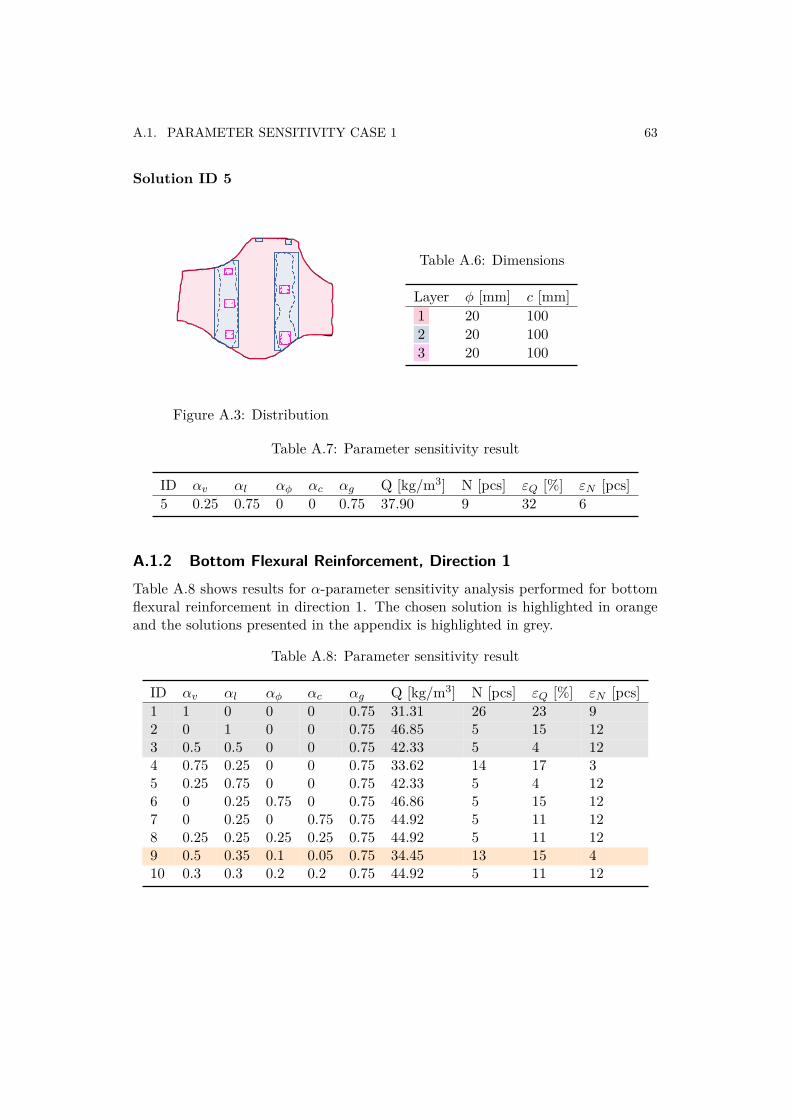
A.1. PARAMETER SENSITIVITY CASE 1 63
Solution ID 5
Figure A.3: Distribution
Table A.6: Dimensions
Layer „ [mm] c [mm]1 20 1002 20 1003 20 100
Table A.7: Parameter sensitivity result
ID –
v
–
l
–
„
–
c
–
g
Q [kg/m3] N [pcs] Á
Q
[%] Á
N
[pcs]5 0.25 0.75 0 0 0.75 37.90 9 32 6
A.1.2 Bottom Flexural Reinforcement, Direction 1Table A.8 shows results for –-parameter sensitivity analysis performed for bottomflexural reinforcement in direction 1. The chosen solution is highlighted in orangeand the solutions presented in the appendix is highlighted in grey.
Table A.8: Parameter sensitivity result
ID –
v
–
l
–
„
–
c
–
g
Q [kg/m3] N [pcs] Á
Q
[%] Á
N
[pcs]1 1 0 0 0 0.75 31.31 26 23 92 0 1 0 0 0.75 46.85 5 15 123 0.5 0.5 0 0 0.75 42.33 5 4 124 0.75 0.25 0 0 0.75 33.62 14 17 35 0.25 0.75 0 0 0.75 42.33 5 4 126 0 0.25 0.75 0 0.75 46.86 5 15 127 0 0.25 0 0.75 0.75 44.92 5 11 128 0.25 0.25 0.25 0.25 0.75 44.92 5 11 129 0.5 0.35 0.1 0.05 0.75 34.45 13 15 410 0.3 0.3 0.2 0.2 0.75 44.92 5 11 12
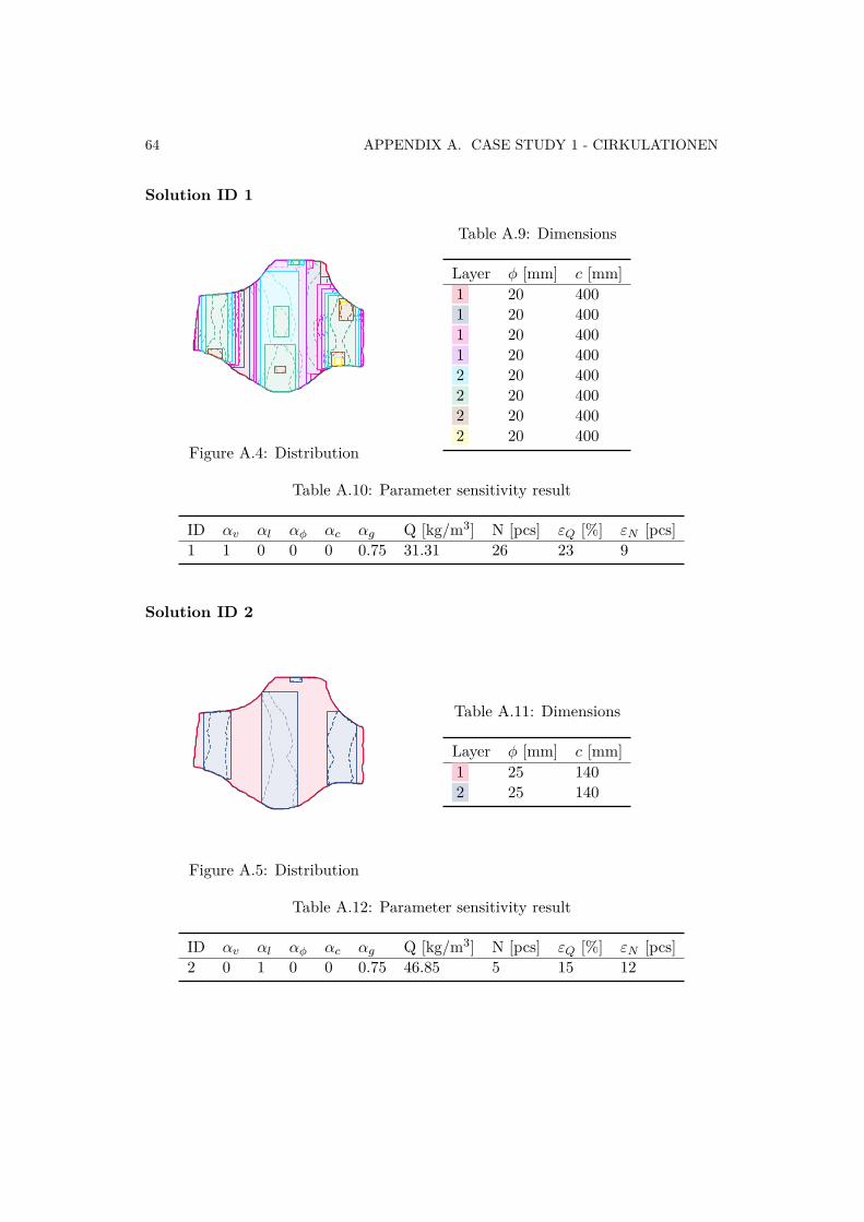
64 APPENDIX A. CASE STUDY 1 - CIRKULATIONEN
Solution ID 1
Figure A.4: Distribution
Table A.9: Dimensions
Layer „ [mm] c [mm]1 20 4001 20 4001 20 4001 20 4002 20 4002 20 4002 20 4002 20 400
Table A.10: Parameter sensitivity result
ID –
v
–
l
–
„
–
c
–
g
Q [kg/m3] N [pcs] Á
Q
[%] Á
N
[pcs]1 1 0 0 0 0.75 31.31 26 23 9
Solution ID 2
Figure A.5: Distribution
Table A.11: Dimensions
Layer „ [mm] c [mm]1 25 1402 25 140
Table A.12: Parameter sensitivity result
ID –
v
–
l
–
„
–
c
–
g
Q [kg/m3] N [pcs] Á
Q
[%] Á
N
[pcs]2 0 1 0 0 0.75 46.85 5 15 12
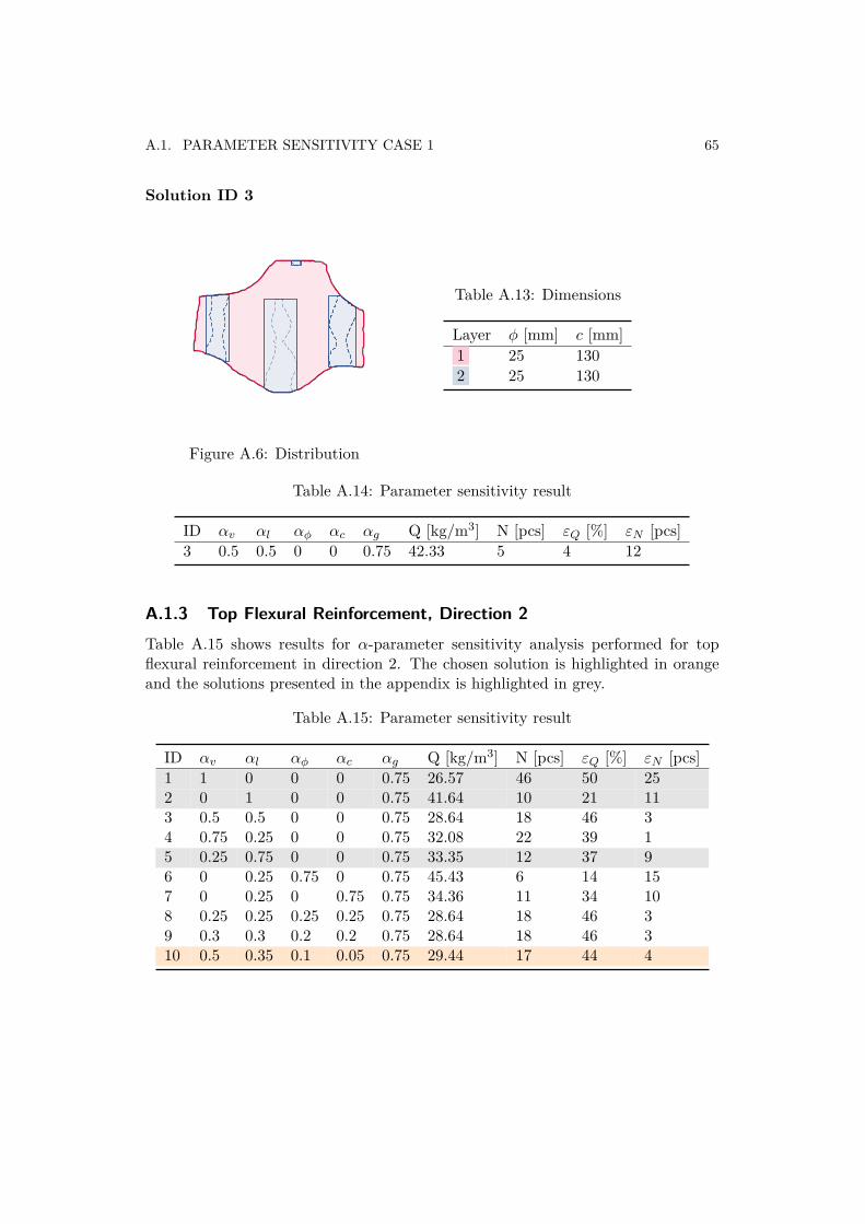
A.1. PARAMETER SENSITIVITY CASE 1 65
Solution ID 3
Figure A.6: Distribution
Table A.13: Dimensions
Layer „ [mm] c [mm]1 25 1302 25 130
Table A.14: Parameter sensitivity result
ID –
v
–
l
–
„
–
c
–
g
Q [kg/m3] N [pcs] Á
Q
[%] Á
N
[pcs]3 0.5 0.5 0 0 0.75 42.33 5 4 12
A.1.3 Top Flexural Reinforcement, Direction 2Table A.15 shows results for –-parameter sensitivity analysis performed for topflexural reinforcement in direction 2. The chosen solution is highlighted in orangeand the solutions presented in the appendix is highlighted in grey.
Table A.15: Parameter sensitivity result
ID –
v
–
l
–
„
–
c
–
g
Q [kg/m3] N [pcs] Á
Q
[%] Á
N
[pcs]1 1 0 0 0 0.75 26.57 46 50 252 0 1 0 0 0.75 41.64 10 21 113 0.5 0.5 0 0 0.75 28.64 18 46 34 0.75 0.25 0 0 0.75 32.08 22 39 15 0.25 0.75 0 0 0.75 33.35 12 37 96 0 0.25 0.75 0 0.75 45.43 6 14 157 0 0.25 0 0.75 0.75 34.36 11 34 108 0.25 0.25 0.25 0.25 0.75 28.64 18 46 39 0.3 0.3 0.2 0.2 0.75 28.64 18 46 310 0.5 0.35 0.1 0.05 0.75 29.44 17 44 4
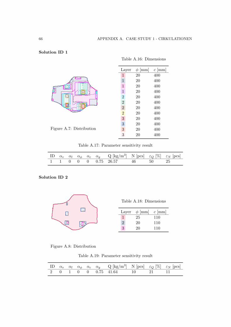
66 APPENDIX A. CASE STUDY 1 - CIRKULATIONEN
Solution ID 1
Figure A.7: Distribution
Table A.16: Dimensions
Layer „ [mm] c [mm]1 20 4001 20 4001 20 4001 20 4002 20 4002 20 4002 20 4002 20 4003 20 4003 20 4003 20 4003 20 400
Table A.17: Parameter sensitivity result
ID –
v
–
l
–
„
–
c
–
g
Q [kg/m3] N [pcs] Á
Q
[%] Á
N
[pcs]1 1 0 0 0 0.75 26.57 46 50 25
Solution ID 2
Figure A.8: Distribution
Table A.18: Dimensions
Layer „ [mm] c [mm]1 25 1102 20 1103 20 110
Table A.19: Parameter sensitivity result
ID –
v
–
l
–
„
–
c
–
g
Q [kg/m3] N [pcs] Á
Q
[%] Á
N
[pcs]2 0 1 0 0 0.75 41.64 10 21 11
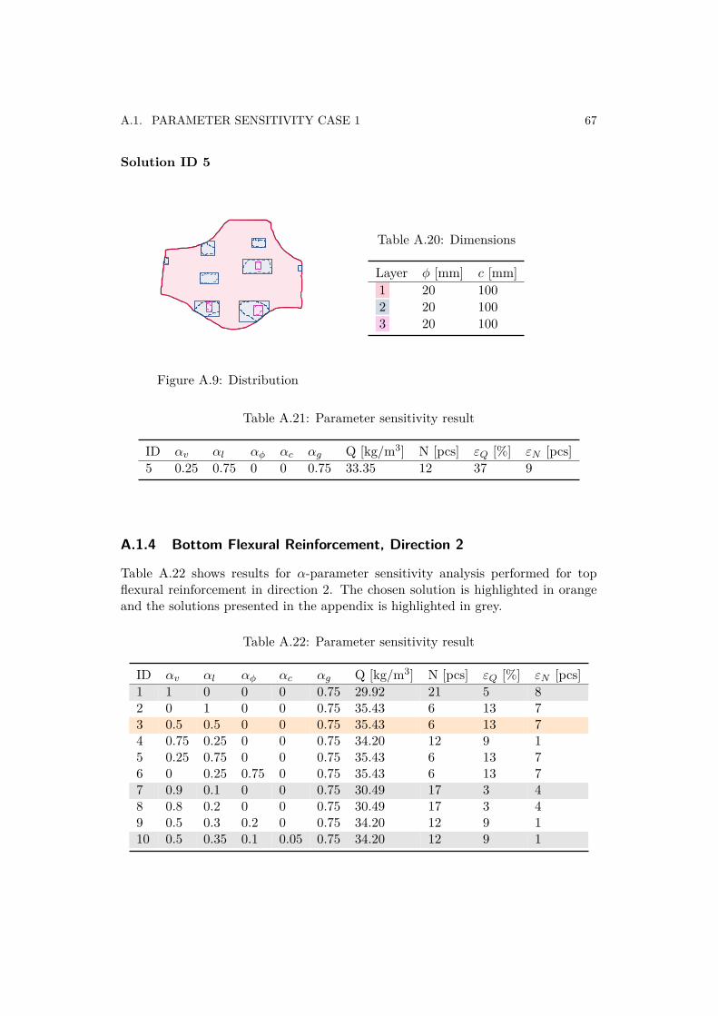
A.1. PARAMETER SENSITIVITY CASE 1 67
Solution ID 5
Figure A.9: Distribution
Table A.20: Dimensions
Layer „ [mm] c [mm]1 20 1002 20 1003 20 100
Table A.21: Parameter sensitivity result
ID –
v
–
l
–
„
–
c
–
g
Q [kg/m3] N [pcs] Á
Q
[%] Á
N
[pcs]5 0.25 0.75 0 0 0.75 33.35 12 37 9
A.1.4 Bottom Flexural Reinforcement, Direction 2
Table A.22 shows results for –-parameter sensitivity analysis performed for topflexural reinforcement in direction 2. The chosen solution is highlighted in orangeand the solutions presented in the appendix is highlighted in grey.
Table A.22: Parameter sensitivity result
ID –
v
–
l
–
„
–
c
–
g
Q [kg/m3] N [pcs] Á
Q
[%] Á
N
[pcs]1 1 0 0 0 0.75 29.92 21 5 82 0 1 0 0 0.75 35.43 6 13 73 0.5 0.5 0 0 0.75 35.43 6 13 74 0.75 0.25 0 0 0.75 34.20 12 9 15 0.25 0.75 0 0 0.75 35.43 6 13 76 0 0.25 0.75 0 0.75 35.43 6 13 77 0.9 0.1 0 0 0.75 30.49 17 3 48 0.8 0.2 0 0 0.75 30.49 17 3 49 0.5 0.3 0.2 0 0.75 34.20 12 9 110 0.5 0.35 0.1 0.05 0.75 34.20 12 9 1

68 APPENDIX A. CASE STUDY 1 - CIRKULATIONEN
Solution ID 1
Figure A.10: Distribution
Table A.23: Dimensions
Layer „ [mm] c [mm]1 25 4001 25 4001 25 4001 25 4002 16 4002 16 4002 16 4002 16 400
Table A.24: Parameter sensitivity result
ID –
v
–
l
–
„
–
c
–
g
Q [kg/m3] N [pcs] Á
Q
[%] Á
N
[pcs]1 1 0 0 0 0.75 29.92 21 5 8
Solution ID 7
Figure A.11: Distribution
Table A.25: Dimensions
Layer „ [mm] c [mm]1 25 4001 25 4001 25 4001 25 4002 16 100
Table A.26: Parameter sensitivity result
ID –
v
–
l
–
„
–
c
–
g
Q [kg/m3] N [pcs] Á
Q
[%] Á
N
[pcs]7 0.9 0.1 0 0 0.75 30.49 17 3 4
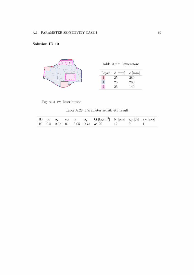
A.1. PARAMETER SENSITIVITY CASE 1 69
Solution ID 10
Figure A.12: Distribution
Table A.27: Dimensions
Layer „ [mm] c [mm]1 25 2801 25 2802 25 140
Table A.28: Parameter sensitivity result
ID –
v
–
l
–
„
–
c
–
g
Q [kg/m3] N [pcs] Á
Q
[%] Á
N
[pcs]10 0.5 0.35 0.1 0.05 0.75 34.20 12 9 1

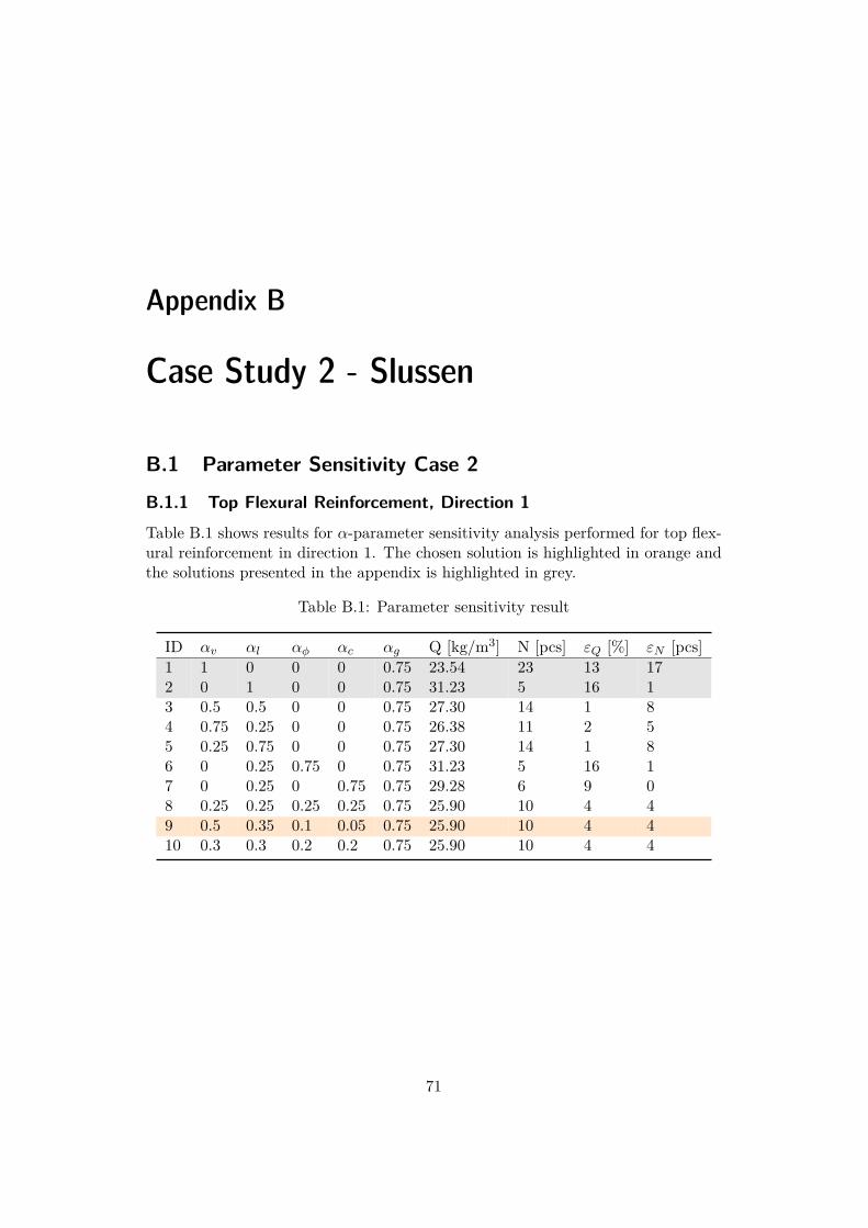
Appendix B
Case Study 2 - Slussen
B.1 Parameter Sensitivity Case 2B.1.1 Top Flexural Reinforcement, Direction 1Table B.1 shows results for –-parameter sensitivity analysis performed for top flex-ural reinforcement in direction 1. The chosen solution is highlighted in orange andthe solutions presented in the appendix is highlighted in grey.
Table B.1: Parameter sensitivity result
ID –
v
–
l
–
„
–
c
–
g
Q [kg/m3] N [pcs] Á
Q
[%] Á
N
[pcs]1 1 0 0 0 0.75 23.54 23 13 172 0 1 0 0 0.75 31.23 5 16 13 0.5 0.5 0 0 0.75 27.30 14 1 84 0.75 0.25 0 0 0.75 26.38 11 2 55 0.25 0.75 0 0 0.75 27.30 14 1 86 0 0.25 0.75 0 0.75 31.23 5 16 17 0 0.25 0 0.75 0.75 29.28 6 9 08 0.25 0.25 0.25 0.25 0.75 25.90 10 4 49 0.5 0.35 0.1 0.05 0.75 25.90 10 4 410 0.3 0.3 0.2 0.2 0.75 25.90 10 4 4
71
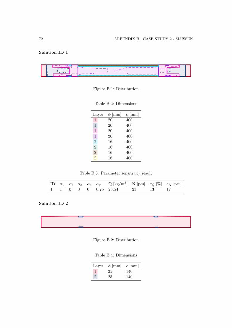
72 APPENDIX B. CASE STUDY 2 - SLUSSEN
Solution ID 1
Figure B.1: Distribution
Table B.2: Dimensions
Layer „ [mm] c [mm]1 20 4001 20 4001 20 4001 20 4002 16 4002 16 4002 16 4002 16 400
Table B.3: Parameter sensitivity result
ID –
v
–
l
–
„
–
c
–
g
Q [kg/m3] N [pcs] Á
Q
[%] Á
N
[pcs]1 1 0 0 0 0.75 23.54 23 13 17
Solution ID 2
Figure B.2: Distribution
Table B.4: Dimensions
Layer „ [mm] c [mm]1 25 1402 25 140
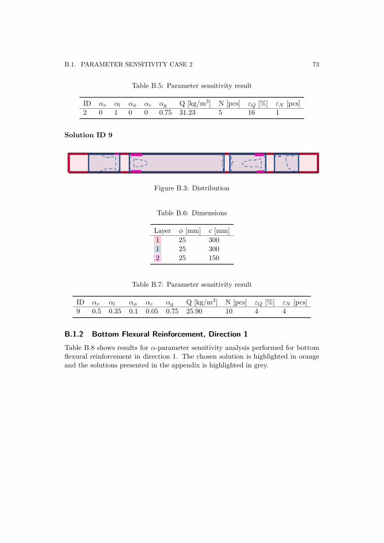
B.1. PARAMETER SENSITIVITY CASE 2 73
Table B.5: Parameter sensitivity result
ID –
v
–
l
–
„
–
c
–
g
Q [kg/m3] N [pcs] Á
Q
[%] Á
N
[pcs]2 0 1 0 0 0.75 31.23 5 16 1
Solution ID 9
Figure B.3: Distribution
Table B.6: Dimensions
Layer „ [mm] c [mm]1 25 3001 25 3002 25 150
Table B.7: Parameter sensitivity result
ID –
v
–
l
–
„
–
c
–
g
Q [kg/m3] N [pcs] Á
Q
[%] Á
N
[pcs]9 0.5 0.35 0.1 0.05 0.75 25.90 10 4 4
B.1.2 Bottom Flexural Reinforcement, Direction 1Table B.8 shows results for –-parameter sensitivity analysis performed for bottomflexural reinforcement in direction 1. The chosen solution is highlighted in orangeand the solutions presented in the appendix is highlighted in grey.
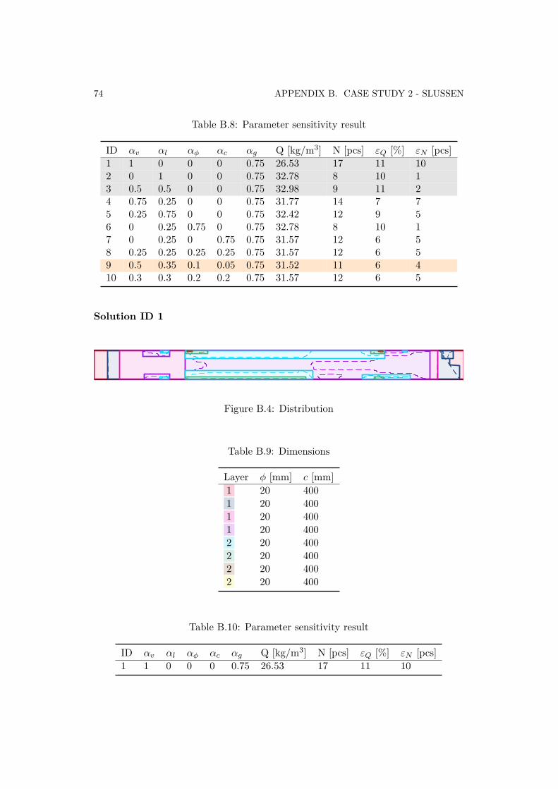
74 APPENDIX B. CASE STUDY 2 - SLUSSEN
Table B.8: Parameter sensitivity result
ID –
v
–
l
–
„
–
c
–
g
Q [kg/m3] N [pcs] Á
Q
[%] Á
N
[pcs]1 1 0 0 0 0.75 26.53 17 11 102 0 1 0 0 0.75 32.78 8 10 13 0.5 0.5 0 0 0.75 32.98 9 11 24 0.75 0.25 0 0 0.75 31.77 14 7 75 0.25 0.75 0 0 0.75 32.42 12 9 56 0 0.25 0.75 0 0.75 32.78 8 10 17 0 0.25 0 0.75 0.75 31.57 12 6 58 0.25 0.25 0.25 0.25 0.75 31.57 12 6 59 0.5 0.35 0.1 0.05 0.75 31.52 11 6 410 0.3 0.3 0.2 0.2 0.75 31.57 12 6 5
Solution ID 1
Figure B.4: Distribution
Table B.9: Dimensions
Layer „ [mm] c [mm]1 20 4001 20 4001 20 4001 20 4002 20 4002 20 4002 20 4002 20 400
Table B.10: Parameter sensitivity result
ID –
v
–
l
–
„
–
c
–
g
Q [kg/m3] N [pcs] Á
Q
[%] Á
N
[pcs]1 1 0 0 0 0.75 26.53 17 11 10
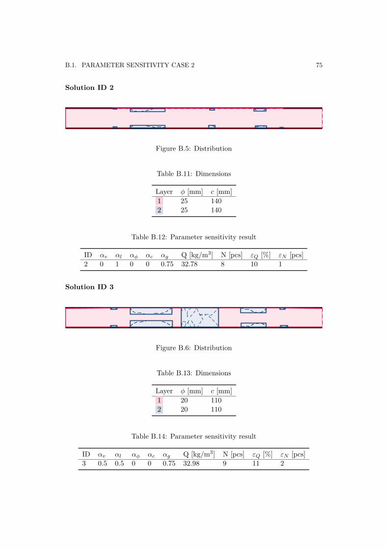
B.1. PARAMETER SENSITIVITY CASE 2 75
Solution ID 2
Figure B.5: Distribution
Table B.11: Dimensions
Layer „ [mm] c [mm]1 25 1402 25 140
Table B.12: Parameter sensitivity result
ID –
v
–
l
–
„
–
c
–
g
Q [kg/m3] N [pcs] Á
Q
[%] Á
N
[pcs]2 0 1 0 0 0.75 32.78 8 10 1
Solution ID 3
Figure B.6: Distribution
Table B.13: Dimensions
Layer „ [mm] c [mm]1 20 1102 20 110
Table B.14: Parameter sensitivity result
ID –
v
–
l
–
„
–
c
–
g
Q [kg/m3] N [pcs] Á
Q
[%] Á
N
[pcs]3 0.5 0.5 0 0 0.75 32.98 9 11 2
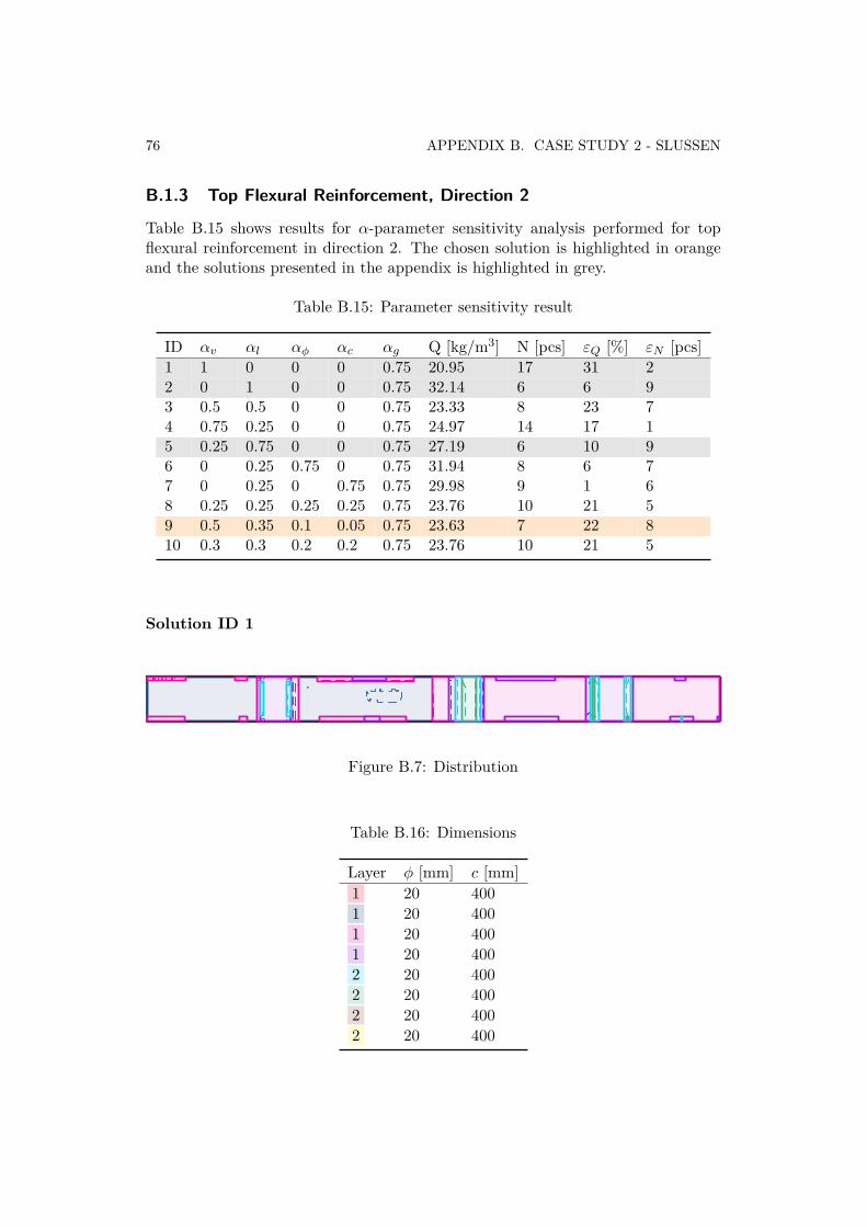
76 APPENDIX B. CASE STUDY 2 - SLUSSEN
B.1.3 Top Flexural Reinforcement, Direction 2
Table B.15 shows results for –-parameter sensitivity analysis performed for topflexural reinforcement in direction 2. The chosen solution is highlighted in orangeand the solutions presented in the appendix is highlighted in grey.
Table B.15: Parameter sensitivity result
ID –
v
–
l
–
„
–
c
–
g
Q [kg/m3] N [pcs] Á
Q
[%] Á
N
[pcs]1 1 0 0 0 0.75 20.95 17 31 22 0 1 0 0 0.75 32.14 6 6 93 0.5 0.5 0 0 0.75 23.33 8 23 74 0.75 0.25 0 0 0.75 24.97 14 17 15 0.25 0.75 0 0 0.75 27.19 6 10 96 0 0.25 0.75 0 0.75 31.94 8 6 77 0 0.25 0 0.75 0.75 29.98 9 1 68 0.25 0.25 0.25 0.25 0.75 23.76 10 21 59 0.5 0.35 0.1 0.05 0.75 23.63 7 22 810 0.3 0.3 0.2 0.2 0.75 23.76 10 21 5
Solution ID 1
Figure B.7: Distribution
Table B.16: Dimensions
Layer „ [mm] c [mm]1 20 4001 20 4001 20 4001 20 4002 20 4002 20 4002 20 4002 20 400
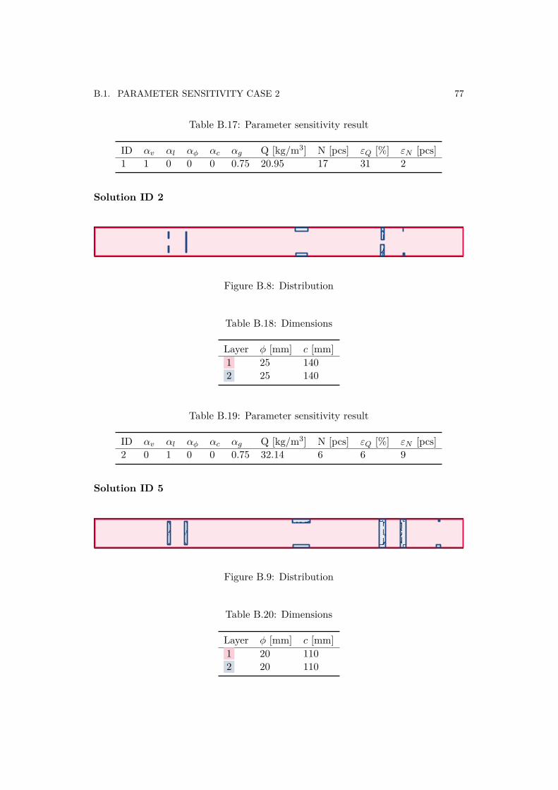
B.1. PARAMETER SENSITIVITY CASE 2 77
Table B.17: Parameter sensitivity result
ID –
v
–
l
–
„
–
c
–
g
Q [kg/m3] N [pcs] Á
Q
[%] Á
N
[pcs]1 1 0 0 0 0.75 20.95 17 31 2
Solution ID 2
Figure B.8: Distribution
Table B.18: Dimensions
Layer „ [mm] c [mm]1 25 1402 25 140
Table B.19: Parameter sensitivity result
ID –
v
–
l
–
„
–
c
–
g
Q [kg/m3] N [pcs] Á
Q
[%] Á
N
[pcs]2 0 1 0 0 0.75 32.14 6 6 9
Solution ID 5
Figure B.9: Distribution
Table B.20: Dimensions
Layer „ [mm] c [mm]1 20 1102 20 110

78 APPENDIX B. CASE STUDY 2 - SLUSSEN
Table B.21: Parameter sensitivity result
ID –
v
–
l
–
„
–
c
–
g
Q [kg/m3] N [pcs] Á
Q
[%] Á
N
[pcs]5 0.25 0.75 0 0 0.75 27.19 6 10 9
B.1.4 Bottom Flexural Reinforcement, Direction 2
Table B.22 shows results for –-parameter sensitivity analysis performed for bottomflexural reinforcement in direction 2. The chosen solution is highlighted in orangeand the solutions presented in the appendix is highlighted in grey.
Table B.22: Parameter sensitivity result
ID –
v
–
l
–
„
–
c
–
g
Q [kg/m3] N [pcs] Á
Q
[%] Á
N
[pcs]1 1 0 0 0 0.75 28.32 23 32 142 0 1 0 0 0.75 44.40 3 7 63 0.5 0.5 0 0 0.75 34.43 10 17 14 0.75 0.25 0 0 0.75 39.88 10 4 15 0.25 0.75 0 0 0.75 41.92 3 1 66 0 0.25 0.75 0 0.75 44.40 3 7 67 0 0.25 0 0.75 0.75 40.58 7 3 28 0.25 0.25 0.25 0.25 0.75 34.43 10 17 19 0.5 0.3 0.2 0 0.75 34.43 10 17 110 0.5 0.35 0.1 0.05 0.75 34.75 7 17 2
Solution ID 1
Figure B.10: Distribution
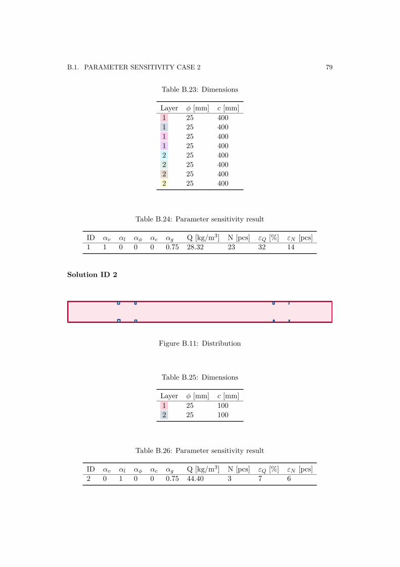
B.1. PARAMETER SENSITIVITY CASE 2 79
Table B.23: Dimensions
Layer „ [mm] c [mm]1 25 4001 25 4001 25 4001 25 4002 25 4002 25 4002 25 4002 25 400
Table B.24: Parameter sensitivity result
ID –
v
–
l
–
„
–
c
–
g
Q [kg/m3] N [pcs] Á
Q
[%] Á
N
[pcs]1 1 0 0 0 0.75 28.32 23 32 14
Solution ID 2
Figure B.11: Distribution
Table B.25: Dimensions
Layer „ [mm] c [mm]1 25 1002 25 100
Table B.26: Parameter sensitivity result
ID –
v
–
l
–
„
–
c
–
g
Q [kg/m3] N [pcs] Á
Q
[%] Á
N
[pcs]2 0 1 0 0 0.75 44.40 3 7 6
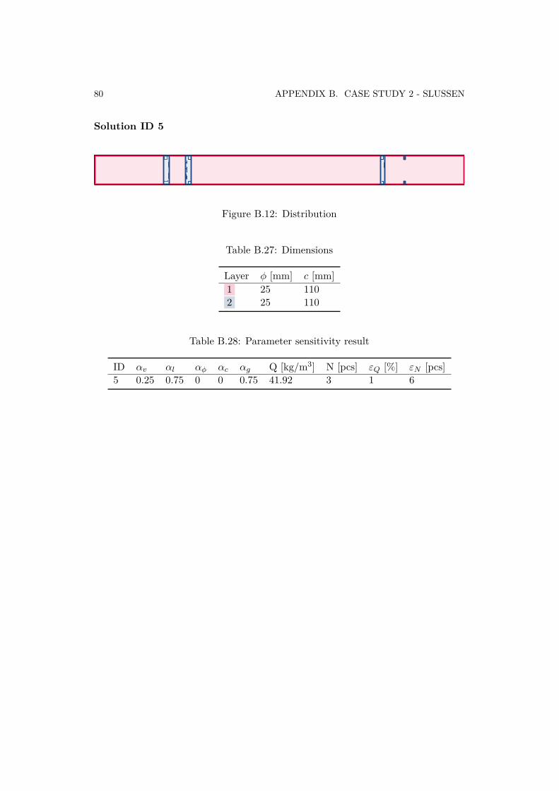
80 APPENDIX B. CASE STUDY 2 - SLUSSEN
Solution ID 5
Figure B.12: Distribution
Table B.27: Dimensions
Layer „ [mm] c [mm]1 25 1102 25 110
Table B.28: Parameter sensitivity result
ID –
v
–
l
–
„
–
c
–
g
Q [kg/m3] N [pcs] Á
Q
[%] Á
N
[pcs]5 0.25 0.75 0 0 0.75 41.92 3 1 6

TRITA ABE-MBT-18301
www.kth.se