An Automatic Visibility Measurement System Based on Video Cameras

Final Report

Prepared by

Taek Mu Kwon, Ph.D

Department of Electrical and Computer Engineering University of Minnesota, Duluth Campus

Duluth, MN 55812

September 1998

Prepared for the

Minnesota Department of Transportation Duluth Office and

Office of Research Administration 200 Ford Buildings Mail Stop 330

117 University Avenue St. Paul, Minnesota 55155

This report represents the results of research conducted by the author and does not necessarily represent the views or policy of the Minnesota Department of Transportation. This report does not constitute a standard, specification, or regulation. ***The original form of this report exists only as a printed copy. This electronic version was reproduced for electronic distribution by Dr. Taek Kwon from the original Mn/DOT’s printed copy. Readers should be aware that the page numbers do not exactly match with the printed version. While conversion, minor editing was also done but without changing the original contents.

Technical Report Documentation Page1. Report No. 2. 3. Recipient’s Accession No.

MN/RC-1998-25 4. Title and Subtitle 5. Report Date

September 1998

6.

An Automatic Visibility Measurement System Based on Video Cameras

7. Author(s) 8. Performing Organization Report No.

Taek Mu Kwon

9. Performing Organization Name and Address 10. Project/Task/Work Unit No.

47

11. Contract (C) or Grant (G) No.

Department of Electrical and Computer Engineering University of Minnesota, Duluth 10 University Dr. Duluth, MN 55812 (C) 74708 TOC # 10

12. Sponsoring Organization Name and Address 13. Type of Report and Period Covered

Final Report – 1996 to 1998

14. Sponsoring Agency Code

Minnesota Department of Transportation 395 John Ireland Boulevard Mail Stop 330 St. Paul, Minnesota 55155

15. Supplementary Notes

16. Abstract (Limit: 200 words)

This report describes a two year study on visibility measurement methods using video cameras. A good theoretical basis and practical methods along with the experimental results are presented. Among several methods and algorithms developed, the edge decay model along with a proper threshold technique worked best for evaluating daytime visibility. This approach estimates the distance where an object of specified size and shape is no longer distinguishable from the background in terms of edge information. For night time, a constant light source is required to evaluate visibility. A light diffusion model that follows an exponential decay curve was developed. It was found that the volume of light diffused out of the original source is logarithmically correlated to visibility. The developed day and night algorithms were implemented in the field and evaluated using manual measurements. For daytime, visibilities measured using the edge decay model closely approximated the manual measurements on all types of weather. For night time, evaluation was very difficult because of unreliability of manual measurements at night. However, it was verified that the trend of visibility change obtained by the proposed approach closely approximates the trend of manual measurements.

17. Document Analysis/Descriptors 18. Availability Statement

Visibility, video camera, visual range, scattering effect, stopping distance.

No restrictions. Document available from: National Technical Information Services, Springfield, Virginia 22161

19. Security Class (this report) 20. Security Class (this page) 21. No. of Pages 22. Price

Unclassified Unclassified 66

ACKNOWLEDGEMENTS The author expresses appreciation to the Office of Research Administration and Mn/DOT

District -1 for financial and manpower support for this research. Special thanks to Mr. Edward

Fleege of Mn/DOT for his tireless help on all phases of the project. Several maintenance engineers

at the Mn/DOT Duluth Office also provided valuable assistance. Thanks also to Mr. Tim Garret of

Castle Rock Consulting Company for providing me large collection of video data from the

previous visibility study.

CONTENTS ACKNOWLEDGEMENTS ................................................................................ i LIST OF TABLES .............................................................................................. iii LIST OF FIGURES ............................................................................................. iii EXECUTIVE SUMMARY .................................................................................. iv I. INTRODUCTION ............................................................................................ 1 II. VISIBILITY CONCEPTS AND TERMINOLOGY ........................................ 5 A. Daytime Visual Range .................................................................................. 5 B. Nighttime Visual Range ................................................................................ 6 C. Meteorological Range ................................................................................... 6 D. Runway Visual Range ................................................................................... 6 E. Recommended Accuracy Requirements ......................................................... 7 III. THEORETICAL DERIVATION OF VISUAL RANGE ................................ 9 A. Basic Principles of Visual Range Based on Contrast ...................................... 9 B. Dual Target Approach ..................................................................................... 10 C. A New Approach Based on Edge and Diffusion Models for Video Images .... 17 IV. IMPLEMENTATION .................................................................................... 25 A. Selection of Video Cameras ......................................................................... 25 B. Target Design ............................................................................................... 26 C. Image Sampling and Software Tools ............................................................. 27 D. User Interface ............................................................................................... 29 V. TESTS AND ANALYSES ON REAL-WORLD DATA ................................. 33 A. Castle Rock Video Data ............................................................................... 33 B. Implementation and Testing in the Field ....................................................... 43 VI. DISCUSSION ................................................................................................. 49 A. Lens Protection from Dirt, Snow, Water drops, etc. ..................................... 49 B. Visibility at Day-to-night or Night-to-day Transition .................................... 50 C. Reduced Visibility by Vehicle Generated Snow Cloud .................................. 50 D. Night Visibility Calibration .......................................................................... 51 E. Remote Control ........................................................................................... 52 F. Speed limit and Visibility relation ................................................................. 52 VII. SUMMARY BY TASKS ............................................................................ 55 VIII. CONCLUSIONS ........................................................................................ 59 REFERENCES ................................................................................................... 61

-ii-

LIST OF TABLES Table 1: Idealized Parameters for Modeling................................................................................................................38 Table 2: Visibility tests on May 30, 1994...................................................................................................................40 Table 3: Visibility tests on June 5, 1994......................................................................................................................40 Table 4: Visibility tests on June 6, 1994.....................................................................................................................41 Table 5: Visibility tests on June 24, 1994....................................................................................................................42 Table 6: Visibility tests on June 27, 1994, Water drops on lens..................................................................................44 Table 7: Visibility tests on February 25, 1994, Snow................................................................................................46 Table 8: Breaking distance on wet pavements (Source from American Association ofState Highway and Transportation Officials (AASHTO))..........................................................................................................................59 Table 9: Stopping sight distance..................................................................................................................................60 Table 10: Suggested speed limit model under various visibility conditions................................................................61

LIST OF FIGURES

Figure 1: Dual target setup for daytime visual range.....................................................................................................9 Figure 2: Dual target setup for nighttime visual range evaluation...............................................................................12 Figure 3: A sample road scene.....................................................................................................................................15 Figure 4: Image of a good visibility night. .................................................................................................................19 Figure 5: 3-D plot of the segmented light target from Figure 4..................................................................................19 Figure 6: 2-D cross-section plot of Figure 5................................................................................................................19 Figure 7: Image of a low visibility night. ...................................................................................................................20 Figure 8: 3-D plot of the segmented light target from Figure 7..................................................................................20 Figure 9: 2-D cross-section plot of Figure 8................................................................................................................20 Figure 10: Target design for a constant light source...................................................................................................25 Figure 11: Target model used in the field implementation.........................................................................................26 Figure 12: Sample screen of the visibility meter implemented. .................................................................................27 Figure 13: Customized visibility data and image loading program. ...........................................................................35 Figure 14: Polynomial visibility model for Sobel estimates.......................................................................................38 Figure 15: Example image that the lens is covered with water drops.........................................................................44 Figure 16: Example of daytime target detection.........................................................................................................49 Figure 17: Example of nighttime target detection. .....................................................................................................49 Figure 18: An example of good daytime visibility (clear day). The image was taken at 11:50AM, June 7, 1997. ....50 Figure 19: Visibility = 147 meters. The image was taken at 8:35AM on July 25, 1997. ............................................51 Figure 20: The visibility is measured at 73 meters. The image was taken at 11:50AM, June 7, 1997. .....................52 Figure 21: Night visibility=210 meters (Image taken at 10:20PM on Aug. 14, 1997) ...............................................53 Figure 22: Data with a good night visibility (image taken at 0:40AM on Aug. 19, 1997) .........................................54

-iii-

EXECUTIVE SUMMARY

This report describes the project entitled “An Automatic Visibility Measurement System Based on

Video Cameras” which was supported by the Mn/DOT MORE fund. The main goal of this project

was to develop a new technique that could measure visibility using video cameras. This design

goal was motivated by the fact that video cameras are used extensively in transportation

applications, and using the same hardware for visibility evaluation could provide a cost effective

solution. In Minnesota, areas with visibility problems identified by Mn/DOT have video cameras

already or will be in place. As an initial step, literature on visibility measurement methods was

extensively reviewed. The research team found that no practical and reliable techniques to

measure visibility using video cameras exist at the present time. Hence, this research embarked on

developing a new set of algorithms for daytime and nighttime visibility using video cameras which

are practical and reliable enough for field use.

The main algorithm developed for daytime is based on the concept that edge information decreases

with distance along with the line of sight. At some point, edges will become extinct. The distance

to the point of extinction is the visibility since the object of given characteristic is no longer

distinguishable from the background. This approach is significantly different from the traditional

approach (i.e. contrast based Koschmieder rule) in that we actually measure how far we can

recognize an object. Therefore, the parameter obtained by this new approach is close to the actual

visibility that a typical human observer may perceive. For nighttime, the amount of volume

diffused out of a constant light source was used. This diffused volume is then modeled using an

exponential decay rule from which an extinction coefficient is derived.

In order to evaluate the algorithms developed, two types of real world test beds were used. The

first test bed was based on a set of real-world highway data collected over a one-year period. This

data set was provided by the Castle Rock Consulting Co. which conducted a study on performance

comparison of commercially available visibility meters against manual measurements. The

second test bed was direct comparison of video visibility against manual measurements in the field

setup. This testing was conducted over a period of two years. The test results showed that the

-iv-

performance of the present video based approach in daytime is as good as the commercially

available scattering based instruments in fog and better in snow as long as the video images are

reliable. For nighttime, manual measurements were extremely difficult. Therefore, the algorithm

was only tuned using very rough estimates. A further study is recommended for night time.

-1-

I. INTRODUCTION

Visibility conditions are affected by the structure and elements of the atmosphere, such as fog,

snow, wind, dust, and other adverse conditions. It is loosely defined as the greatest distance at

which an object of specified characteristics can be seen and detected with the naked eye [1,2,8]. It

is expressed in meters or yards, or at greater ranges, in kilometers or miles. At night, it is

determined by measuring the distance from a point of light of a given intensity to the point where

the light source is just noticeable.

Visibility information provides an identifiable target distance from which we can derive safe speed

limits by incorporating breaking distances per speed. Consequently, visibility is one of the

important determinants for safe driving.

Traditionally, visibility has been evaluated manually or by using commercial visibility instruments.

The latter are constructed based on the principle of measuring forward or backward

light-scattering effects. The main advantage of the scattering based instruments is the capability of

evaluating nighttime visual range without modification from the daytime setup. However, several

drawbacks should be noted and are listed below:

• Visibility is not only reduced by the scattering effect but also by absorption. Hence

measuring scattering alone accounts for only a partial view of the atmospheric

visibility effects.

• Visibility measured by the scattering instruments represents a single spot; thus,

covering a large area requires many repeated installations, which can greatly

increase the overall cost.

• Scattering based instruments show a high margin of error under snow and rain while

they are relatively accurate under fog. This is due to a less significant relation of

visibility to the scattering effect under snow or rain. This observation was pointed

out by Castle Rock's study [5] whereby several commercial visual-range sensors

-2-

failed to recognize low visibility caused by snow. This inconsistency of errors could

pose a problem in practical implementation because it may require different

calibrations under different weather conditions.

• Scattering instruments only measure visual-range, not visibility. This means that

visibility perceived by human eye could be significantly different from the visual

range measured by the scattering based instruments.

• There are no easy ways to verify the correctness of the measured visual range. Video

cameras are frequently used to verify correctness of the measurements, but it greatly

increases the instrumentation and communication cost.

• The scattering based instruments are relatively expensive.

The above are not an exclusive list, but they are the items of concern when scattering based

commercial instruments are used as the visibility sensor in transportation. As an alternative to the

scattering-based instruments, video cameras offer an attractive solution for evaluating visibility.

The reasons are summarized below, and are the subject of this study in which we will explore and

develop useful techniques.

• Since many video cameras are already installed and used for transportation

applications, it provides a low cost solution for visibility evaluation if the same

hardware is used.

• Video cameras display a view along the line of sight instead of a single spot, so that it

represents a large area and provides an estimate less prone to drastic local errors.

• The camera lens system has the same structure as the lens system of human eye. Thus,

it provides an opportunity for measuring perceptual visibility.

• Video information on the actual scene can be obtained as a byproduct of the

approach which would provide an opportunity to verify the measured visibility by

manual inspection.

• In Minnesota, all areas with visibility problems have video cameras already in place.

The above are a list of the advantages that a video camera-based approach may have over the

light-scattering based approach. However, there are some disadvantages of video-based approach

-3-

that should be noted. These include: 1) images can be distorted by dirty lenses; 2) images are

sensitive to lighting conditions; 3) objects are not identifiable at night; 4) images can be blurred by

poor focusing.

Despite some difficulties associated with video cameras, the advantages clearly outweigh the

disadvantages. The researcher believes that it is essentially the ultimate approach to resolve the

visibility issue, because the information seen by the human eye has the same principle as the

information generated by a video camera. Therefore, we have an opportunity to explore the

various methods and principles that could derive what a human observer may perceive the

visibility.

II. VISIBILITY CONCEPTS AND TERMINOLOGY

Measuring visibility is inherently difficult because it involves a measurement of the perceptual

process of human eye, i.e. object recognition. As of today, it is still not well understood how we

recognize objects. For example, identification rate can be increased with prior knowledge about

the object, and quantization of such phenomenon is very difficult. In order to avoid such problems

scientists evaluate another parameter called the visual range in place of visibility. This is defined

by a just minute difference of a black target against the horizon measured by the contrast ratio. In

this concept, visual range is only evaluated by measuring the atmospheric attenuation of contrast,

and scientists and engineers are no longer concerned about human perception. The following

summarizes the basic terminologies related to visual range [1,13].

A. Daytime Visual Range

Daytime visual range is evaluated based on an assumed minimal contrast ratio (0.02 - 0.05, we

adopt 0.05 based on the recommendation by the National Bureau of Standards [8]) for a black

target of a “reasonable” size silhouetted against the horizon viewed by a typical human eye. A

reasonable size by this definition is an object that subtends an angle of 0.5-1.0 degree of arc from

the observer. Under these conditions, visual range V is estimated from the average extinction

coefficient σ using the Koschmieder equation:

V =

3 0.σ (1)

where V is the visual range in meters if σ is in m-1.

-4-

B. Nighttime Visual Range

The nighttime visual range is evaluated based on the minimum amount of lights falling on the

observer's eye which produces a recognizable sensation of brightness. It is governed by the

Allard's law, which is expressed by

E

IeVth

V

=−σ

2 (2)

where Eth is the threshold illuminance detected at the visual range V by a light source of intensity I.

C. Meteorological Range

Meteorological Range is an empirically consistent measure of visual range; a concept developed to

eliminate from consideration of the threshold contrast and adaptation luminance, both of which

vary from observer to observer. For practical purposes one may calculate meteorological range in

the same manner as the daytime visual range relation given in Eq. (1). This formulation satisfies

the requirements of meteorologists since it yields a one-to-one correlation with atmospheric

transmittance, and a change from day to night does not produce a change in the visual range.

D. Runway Visual Range

The maximum distance along the runway at which the runway lights are visible to a pilot after

touchdown. Runway visual range may be determined by an observer located at the end of the

runway, facing in the direction of landing, or by means of a transmissometer installed near the end

of the runway.

-5-

-6-

E. Recommended Accuracy Requirements

The accuracy requirements recommended for visibility measurements are specified in World

Meteorological Organization (WMO) Publication No. 8, “Guide to Meteorological Instruments

and Methods of Observation,” 5th Ed., 1983. It includes the error requirements for aeronautical

and meteorological applications but does not include the requirements for ground level

transportation applications. The requirements for runway visual range may be closely related to

the highway transportation applications, in which the allowable errors are defined

as ±25 meters up to visibility 150 meters; ±50 meters for visibility between 150 to 500 meters; and

±100 meters for visibility between 500 to 1000 meters, and ±200 meters for visibility above 1000

meters.

III. THEORETICAL DERIVATION OF VISUAL RANGE

This section presents theoretical derivations of visual-range algorithms studied in this project. The

fundamental theory of visual range based on contrast is reviewed. New approaches are derived

from the basic theorem.

A. Basic Principles of Visual Range Based on Contrast

Let the luminance of a target be Bt and the horizon background surrounding the target be Bh, then

the contrast C is defined as

C

B BB

t h

h=

−

. (3)

With this definition, contrast may be either positive or negative, with negative meaning that the

target is less luminous than the background. According to Duntley [4], the contrast ratio is

governed by the following rule:

CC

e d

0= −σ

(4)

where C0 is the inherent contrast against sky (i.e the contrast measured at the target), C is the

apparent contrast of the target observed from distance d, and σ is the light attenuation coefficient

(called the extinction coefficient). Visual range V is then defined at the distance where the contrast

ratio falls down to C/C0 = ε0=0.05;

(5) 0 05. = −e Vσ

If σ is obtainable through a transmissometer, visual range is simply computed from Eq. (5) as:

-7-

V =

−=

ln .εσ σ

0 3 0

(6)

If the contrast ratio C/C0 at distance d is measurable, its visual range is computed by substituting σ

in Eq. (4) to Eq. (6), i.e.

Vd

CC

=⋅3 0

0

.

ln (7)

B. Dual Target Approach

Daytime Visual Range

Direct measurement of inherent contrast C0 in Eq. (7) is not simple, because the contrast must be

measured against sky which is infinite while the measurement has to incorporate the dependency

of contrast in light-intensity and weather conditions. To avoid such a difficulty we develop a

dual-target approach that removes the requirement of measuring the inherent (reference) contrast

C0. The basic principle of theory is derived by assuming that two targets are set up at distances d1

and d2 against horizon as shown in Fig. 1. At the observation point of the diagram, an observer or

an instrument measures the contrast of the two targets. Let the measured contrasts be C1 and C2 for

each target, respectively. Then, using Eq. (4) we have

-8-

Figure 1: Dual target setup for daytime visual range.

σ =

1

1

0

1dCC

ln (8)

σ =

1

2

0

2dCC

ln . (9)

Solving for C0 from Eqs. (8) and (9) gives,

-9-

ln ln lnC

dd d

Cd

d dC0

2

2 11

1

2 12=

−−

− . (10)

Finally, substituting Eq. (10) to Eq. (7) yields the visual range we wish to calculate without using

the reference contrast:

Vd d

CC

=− −( )( ln )

ln

2 1 0

1

2

ε

. (11)

Notice from Eq. (11) that the formula consists of no C0 but all easily measurable values. Moreover,

since the contrast values only appear as a ratio (i.e. C1/C2 ), any contrast measurements are valid as

long as the lighting conditions are consistent for both targets. In other words, brightness change

during the day or automatic iris adjustments will not influence the accuracy of the visibility

computation as long as the both targets are under the same atmospheric conditions. On the other

hand, we learned that creating such a condition is hard to obtain. For example, light attenuation

coefficients of atmosphere can be inconsistent within a short distance.

In our case, since the contrasts of two targets are measured from a video image, it is

simultaneously recorded in the same image. Hence, it is temporally consistent as well as spatially

(i.e. the photo-cells at each pixel location is consistent). However, since atmospheric

inconsistency can not be controlled, a short separation distance between the two targets is

recommended in order to minimize the atmospheric inconsistency.

It should be noted that a video image is a collection of pixel values some of which are saturated to

upper or lower limits. Grey scale resolution of each pixel is generally limited to 256 levels (8-bit).

Because of these limits, directly computing visual range using Eq. (11) is prone to a large error,

depending on the resolution and the linearity of luminance of the pixel values. Consequently, some

adjustments must be made to Eq. (11) to minimize the effect; the following is suggested:

-10-

V

C C=

−β

ln ln1 2 (12)

where β is a constant factor that must be calibrated through manual verification of visibility. This

adjustment is necessary to establish a mapping relation between the pixel value and the actual

luminance. In Eq (12), if the contrast of target-2 is reduced with respect to target-1, the visibility is

reduced proportionally in a log scale. This follows the Duntley's law in Eq. (4).

Nighttime Visual Range

Nighttime visual range is defined as the greatest distance at which a point of light-source of the

given candle-power can be perceived at night by an observer under the given atmospheric

condition. Nighttime visual range is limited by the atmospheric attenuation of luminous flux

density as described by the Allard's law in Eq. (2). Let Eth be the luminance threshold that is just

noticeable from the visual range V, then rewriting Eq. (2) gives

EI

V eth V2 = −σ

(13)

The nighttime visual range [2] is then simply derived by solving for V from Eq.(13), i.e.,

V

IE

Vth

= −1

2σ

(ln ln ) (14)

Unfortunately, the relationship in (14) is impractical for visual-range computation, since the light

attenuation coefficient σ is unknown (must be measured) and the luminance threshold Eth must be

adjusted under different lighting conditions. Therefore, we develop a dual-target approach similar

to that of the daytime visual-range, which does not require either Eth or σ. Suppose that two targets

-11-

are set up at distances d1 and d2 with an identical light intensity (unfocused light source) as shown

in Fig. 2. Let the luminance of the two targets detected at the observation point be E1 and E2,

respectively. Then, for each target, the following relations hold:

E

Id

e d1

12

1= −σ

(15)

E

Id

e d2

22

2= −σ

(16)

Solving for σ from Eqs. (15) and (16) gives

σ =

−1

1 2

2 22

1 12d d

E dE d

ln (17)

Figure 2: Dual target setup for nighttime visual range evaluation.

-12-

Notice that E1, E2, d1, and d2 are all known or measurable values. This means that we can derive

the light attenuation of atmosphere if two identical light sources at different locations are available.

Using Eqs (17) and (14), we arrive at a measurable nighttime visual range as:

Vd d

E dE d

V=−

−( )

ln( ln )1 2

2 22

1 12

2ε

(18)

where ε is determined through field experiments.

Further simplification is necessary in order to remove the recursive relation in Eq. (18) , i.e.

V(d d )

E dE d

≈−1 2

2 22

1 12

α

ln (19)

where α is a multiplication factor that is required by just noticeable light source. If sufficient data

can be collected, a sophisticated model can be further developed using the key variables. Let the

variables be

D d dd = −1 2

D EE = −ln ln1 2E

N E

The visibility is then conveniently modeled through an Nth order polynomial, i.e.

(20) V a a D b b D b D b Dd E EN= + + + + + +0 1 0 1 2

2 . . .

-13-

-14-

The coefficients are commonly solved using iterative methods such as a least squares method.

Comments on Night Visibility

In reality, measuring visibility at night is extremely challenging whether it is manual or automated

system. Middleton best describes this difficulty in his famous book, Vision Through the

Atmosphere [2] as follows: “If observation in daytime have their difficulties, these are negligible in

comparison with those encountered at night.”

Ideally, we want to have a camera that gives a parameter linear to the light intensity of targets.

However, video cameras in general are designed to work best for capturing daytime images and

not for detecting light-intensity at night. We found that the pixels of the video camera tend to

saturate quickly against any light source due to the high contrast against dark background at night.

Therefore, we believe that the method developed in Subsection III.B is more appropriate for the

sensors that exhibit a large linear region against light intensity. In the next section, we show new

approaches that are more applicable for video cameras.

C. A New Approach Based on Edge and Diffusion Models for Video Images

Daytime Visibility Derivation Using Edge Information

This approach utilizes the perceptual degradation of an image along the line of sight that

corresponds to actual distances from the observation point. For example, tree lines or fence lines

along the highway can form a continuous degradation model along the straight line of sight from

which extinction of contrast may be detected at some point along that line. To be more specific,

consider the sample road scene shown in Figure 3, where the right side along the edge strip is

chosen for processing. Let the localized contrast along the ideal line be denoted C(d), then it is an

exponentially decreasing function due to the contrast reduction principle in Eq. (4):

(21) C d k C e d( ) = ⋅ −0

σ

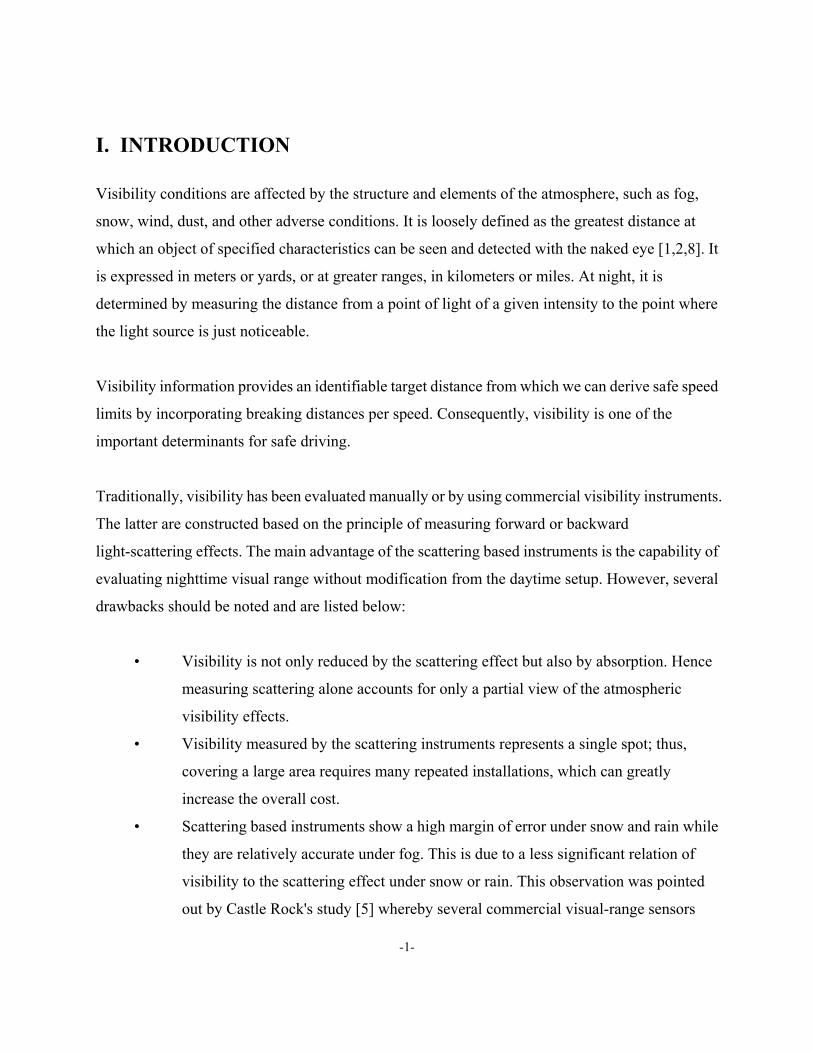
where k is a scaling factor. It should be mentioned that this relation is a rough approximation of

real contrast due to the limits imposed on each pixel and existence of non-ideal continuous targets.

Figure 3: A sample road scene.

For the evaluation of localized contrasts at pixel location (i,j), the following formulation can be

used by incorporating the contrast definition given by Eq. (3):

C i j

p i j pP

av

av( , )

( , )=

−

(22)

where p(i,j) denotes the pixel value at location (i,j) and pav is the average of the pixel values

surrounding the location (i,j). At this point, we may depart from the traditional computation of

-15-

contrast. It is well known that the human visual system inherently utilizes edge information

for object recognition, as is readily evidenced by the way we recognize cartoon pictures.

Hence, it is more logical to utilize the degree of edge information for visibility evaluation than the

contrast by luminance. Thus, we replace the contrast computation in Eq. (22) with an edge

operator. A well known edge operator that has been successfully used in many applications is the

Sobel operator [6], which is given by

-16-

2

(23) S m n d dx y( , ) ( ) /= +2 2 1

where

d p m n p m n p m np m n p m n p m n

d p m n p m n p m np m n p m n p m n

x

y

= − − + − + + − −− + + + + + +

= + − + + + + +

− − + − + − +

( ( , ) ( , ) ( , ))( ( , ) ( , ) ( , )),

( ( , ) ( , ) ( , ))( ( , ) ( , ) ( , )).

1 1 2 1 1 11 1 2 1 1 1

1 1 2 1 1 11 1 2 1 1 1

−

It should be mentioned that other edge operators may be equally eligible for this application, i.e.,

the performance difference by the choice of different edge operators is negligible in this case.

The Sobel values essentially approximate the gradient of an image by a difference operator.

Notice that both the contrast in Eq. (22) and the gradient in (23) include differential terms. This

implies that both in essence represent the same characteristics, i.e. gradient but in different scale.

Next we map the two-dimensional Sobel data to a one dimensional representation by selecting a

maximum edge from each orthogonal direction along the line of sight. The reason for this is to

construct the model based on the best edges. Let the maximum edge values along the line-of-sight

be represented by . We experimentally found that follows the following exponential

rule:

$( )S d $( )S d

$( ) ( )S d

Ke

Kd d=+

+−1

01 0α (24)

where d is the distance from camera to target, and α is a parameter that controls the slope of the

curve, and d0 is the displacement of sloped region. Finally visibility is determined at the

threshold as $S th

V d

KS Kth

= −−

−01

0

11

αln( $ ).

(25)

This new approach is particularly suitable for measuring visibility on highways, since objects

along the straight line-of-sight usually exist (such as tree lines, fence, side ditches), or artificial

targets can be easily placed. One particular advantage of this method is that it is minimally

sensitive to the types of targets. For example, if we choose a tree line along the roadway, no

maintenance of targets will be required, and will be free of errors due to minor target damages or

distortions.

Nighttime Visual Range

Since nighttime visual range is defined by a distance where a light source is just noticeable, the

availability of a light source and a light-intensity meter is prerequisite for nighttime visual-range

measurements. In this project, the average pixel value of a light source in a video image was

initially used as the intensity. After many trial and error of using a video-camera for a

light-intensity measurement, we recognized that directly measuring light intensity from video

images cannot work. This is due to the fact that, characteristically, many video cameras use charge

coupled devises (CCD) which tend to quickly saturate at the location of light source. This quick

saturation is caused by the very high contrast existing between the light source and the total dark

background, leaving only a very narrow linear range. Therefore, we concluded that a new

-17-

approach must be developed for nighttime visual-range if we are going to use a video camera.

After many experiments, we found one characteristic that closely relates to light intensity which is

useable for night visibility. It was the amount of diffused volume out of the saturated region of the

light source. According to our observation, the diffusion volume was increased as visibility

decreased. This phenomenon is clearly shown in Figs. 4- 6 and 7-9 where Figs. 4-6 show a good

visibility example and Figs. 7-9 show a bad visibility example (about 200 meters). The three-D

graphs show the light intensity profile, and the two-D graphs show the cross-section. Notice that

Fig. 5 has almost no diffused lights while Fig. 8 has a lot of diffused lights. If we plot the

cross-section of the diffused area, it follows exponential curves as shown in Figs. 6 and 9. In

general, the following relation holds:

. (26) F d F e d( , )η η= −0

We will call η as the diffusion coefficient and F as the diffusion curve. In order to relate Eq. (26)

with the traditional formulation, let's assume that we measured an identical light source under two

different extinction coefficients, σ1 and σ2. Let the measured light intensities at a distance R be E1

and E2, respectively to σ1 and σ2. Then, the following relation can be derived using the classical

Allard's law in Eq. (2):

E E

ER

e eR R1 2

02

1 2− = −− −( )σ σ

. (27)

-18-

Figure 4: Image of a good visibility night.

Figure 5: 3-D plot of the segmented light target from Figure 4.

Figure 6: 2-D cross-section plot of Figure 5.

-19-

Figure 7: Image of a low visibility night.

Figure 8: 3-D plot of the segmented light target from Figure 7.

Figure 9: 2-D cross-section plot of Figure 8.

-20-

Now, let's further assume that we derived two diffusion curves on the same light source under the

same extinction coefficients σ1 and σ2 as in Eq. (27). Let the diffusion values measured be F1 and

F2 at distance d, then we have,

F F

FR

e ed d1 2

02

1 2− = −− −( )η η

(28)

where η1 and η2 are the computed diffusion coefficients using the basic diffusion model in Eq. (26).

From Eqs. (27) and (28), we have the following relation

η σd = R (29)

Since both d and R represent distances, we can derive the visual range by setting a threshold Eth as

the reference. In conclusion, nighttime visual range holds the following relation with respect to the

diffusion coefficient:

V ∝η (30)

or can be computed by

V k= ⋅η (31)

where k is a constant scaling factor. This linear relation holds in most of the visual ranges.

However, if some areas do deviate from this linear relation, we can always introduce a polynomial

mapping function, i.e.

V f p= ( )η (32)

where is a polynomial function. f p ( )⋅

-21-

-22-

-23-

IV. IMPLEMENTATION

This section describes implementation of the theory into practice where various hardware,

software, and communication issues are involved.

A. Selection of Video Cameras

With the advances in imaging technologies, video cameras can capture sufficient resolution of

images suitable for visibility evaluation. Ideally, we would like to have a camera that can simulate

the characteristics and functions of human eye. As a general rule, cameras with the following

features are recommended:

• Auto iris. Iris automatically controls the amount of light. It is generally controlled

through the exposer time in CCD Cameras.

• High resolution. The human eye has much higher resolution than present video

camera resolutions. One way of overcoming this problem is through the use of

telephoto lenses to compensate the lack of resolution in the video camera.

• Back light compensation. An automatic back light compensation function is

desirable to minimize the drastic contrast drop at the objects when the camera is

against sunlight.

• Defrost heater and fan. During cold winter weather or damp summer days, frost or

fog on the lens can severely degrade the quality of an image. Heaters and cooling

fans are required to defrost or defog the camera lens.

• Automatic lens cleaning function. Snow, mud, dust, etc., on the lens can severely

distort the image. An automatic cleaning function or a protective mechanism is

required to maintain the lens clean.

-24-

B. Target Design

How to design the target model is important, but it is not a critical factor to the performance as long

as some common senses described below are applied. The following guidelines are recommended.

• At least one target must include a constant light source for night visibility.

• The size of the targets must appear approximately the same size in the video image.

This is achieved by increasing the size of the targets as the distance to the

observation point increases. As a rule of thumb, targets must be subtended about 0.5

degree with respect to the distance.

• About five targets spaced up to 300 meters from the camera are recommended. This

is to allow accurate measurement of visibility up to 300 meters, which is considered

an important range for highway applications.

• All targets must be visible in one screen.

• Targets must have black background and white stripes. The white stripes against the

black background create strong contrast and edge information desirable for good

visibility measurements. Anything other than white color can fail when the ground is

covered with snow. It is important to recognize that white snow can create a strong

false edge or contrast that can dominate the true edge or contrast information.

In our implementation, six targets were used, and two of them housed a constant light source. The

targets were spaced 20m, 40m, 100m, 150m, 200m, and 300m. The target at 20m was installed for

the initial dual-target approach introduced in Section III and does not contribute to the current

computational model implemented in the field. However, it serves as a reference point for target

search. The design of target with light source and the rest of the target dimension and pattern are

shown Fig. 10 and 11, respectively.

Figure 10: Target design for a constant light source.

C. Image Sampling and Software Tools

For sampling video images, a Snappy developed by the Plays Corp. was used. This digitizer is

designed for still images and is connected through a printer port. The sampling time is about 6

seconds due to the slow speed of the printer port. A customized, automated data collection

program and a snapshot program were written using a C++ language for this research. Most image

sampling was done at intervals of five minutes.

-25-

Figure 11: Target model used in the field implementation.

For the development of algorithms and implementation in the field, an Interactive Data Language

(IDL) package was used as the basic language tool. The IDL provides a rich set of image

processing routines that are very useful for implementing present application.

In order to remotely access the computer in the field, a modem and a LapLink from Traveling

Software Co. were used. Initially, pcAnywhere from Symntec was used, but it caused frequent

lock up of the remote computer and modem. The LapLink performed better under unstable phone

lines and provided a better file transfer speed. In order to take an advantage of the file transfer

capability of LapLink, a JPEG file viewing program that also shows the visibility computed at the

field was developed.

-26-

Figure 12: Sample screen of the visibility meter implemented.

D. User Interface

The final form of user interface developed for this project is shown in Figure. 12. The primary

goal was to develop a user-friendly interface which provides essential information that could lead

to a better decision-making process with respect to visibility.

The image provided in the window allows manual verification. The graph in the right side window

provides a mathematical modeling of the visibility which can be used to verify the correct curve

fitting of the data.

The function of each button in the window is described below.

Snap Press this button to sample a picture using the Snappy digitizer. It digitizes

and creates a 640X480 color bitmap-image, and then saves it as a file

“tmpidl.bmp” which is later used by the other routines. This button would

be the first to press if one wishes to check the current visibility.

-27-

34

Comp Snapped Pressing this button will cause two actions. First, the color image grabbed

by Snap (stored in “tmpidl.bmp”) is converted to a gray scaled 320X240

image and displayed in the left side of the window. Next, visibility is

computed, and the result is displayed using a pop-up message box.

Load/Comp This button loads an image from a storage selected by a user and computes

its visibility. The result is displayed using a pop-up message box. This

button is useful when the user wants to check images sampled in the past.

Compute Vis It computes the visibility of the image available in the current buffer. It can

be used after Comp Snapped or Load/Comp to recheck the visibility.

Targets This button is used to see how the algorithm searches the targets. Pressing

this button will display the searched result of the targets in the right side of

the window. This routine is useful to check the target search-algorithm and

to calibrate the camera angle to the targets.

Save as JPEG This routine converts the image available in the current buffer to a JPEG

color image (320X240) and saves it at “C:\imagex\download.jpg”. This file

is created for the LapLink’s automatic file synchronization utility to allow

effective downloading to a local computer.

Exit Ends the current session.

The above program resides in the remote computer which is accessed though a LapLink remote

control program from a local computer. Downloading of the captured image is done through the

LapLink’s Automatic File Synchronization utility. Although images can be downloaded, there is

no simple way to display the downloaded images along with the measured visibility at the local

computer. Therefore, another utility program was created in order to decompress the downloaded

JPEG image and display the measured visibility. A sample screen of this program is shown in Fig.

13

Figure 13: Customized visibility data and image loading program.

35

36

V. TESTS AND ANALYSES ON REAL-WORLD DATA

This section describes the tests and analyses of the developed visibility algorithms on real-world

data. The first set of data was provided by the Castle Rock Company and served as the resource for

trying out various algorithms and developing new visibility evaluation techniques. Experimental

results of Castle Rock’s data are described in Subsection V.A. The field tests conducted are

discussed in Subsection V.B.

A. Castle Rock Video Data

During the period from 1993 to 1995, Castle Rock Consulting firm tested several commercially

available visibility sensors in a real world setting. The goal of this testing was to analyze the

performance (accuracy and robustness) of each sensor against manual measurements. During this

testing, video images were captured for verification and analysis purposes [5] and became the

initial source of this study. In order to manually evaluate the visibility, the research team installed

nine targets which were at distances: 5, 10.5, 20.1, 32.7, 67, 80, 100, 150, and 200 meters. The

targets were numbered 1 though 9 for identification purpose. (See Fig. 3 in Section III.)

Before the analysis of Castle Rock’s video data, a number of aspects must be taken into

consideration. First, the manual measurements recorded in the data themselves had a large margin

of errors due to the limited number of targets. For example, at 150 meters, the error range is about

50 meters, since the next target available is at 200 meters. Second, the research team used identical

target sizes for all targets regardless of the distance, such that targets located farther away were

difficult to recognize or at least not given a fair chance of recognition rate. Third, in order to make

a fair analysis, we wanted to have the data chosen from many different visual ranges and under

different weather conditions. Ideally, this would include an equal number of samples from

visibility near zero to two hundred meters from various weather conditions. Unfortunately, nature

did not allow such an ideal data set. Indeed, the population of actual data was heavily biased, i.e.,

the data set was mostly concentrated in foggy conditions, and only one day for snow and no data

for rain. Forth, some of the images were distorted by out-of-focus or water drops in the lens.

However, these imperfect data helped develop a more robust algorithm.

As an initial test, the dual target approach developed in Section III was tested for all available

images. The dual target approach worked well as long as the extinction coefficients were similar

in both target areas. However, when the extinction coefficients were significantly different, it

failed badly. We found that such conditions occur more frequently if the distance between two

targets is larger. Another factor that influenced this method was distortion of image by water drops

in the lens. If water drops appear at the target regions, a false contrast is measured for the affecting

targets. Thus, the visibility computation significantly deviated from the real visibility. Later we

realized that the log difference appears in Eq. (12) works as a noise or distortion amplifier for

distorted images. After many experiments, we concluded that this method is not robust enough and

not appropriate for video images.

After trying many ideas, we came to the conclusion that we need to develop a method that filters

the localized errors. This direction led to a new theoretical model derived in Section III.C. In this

approach, the main idea is to fit the imperfect data into a perfect model, such that the outliers of the

data are ignored. The test of this idea was done through calculating the Sobel operator given in Eq.

(23) in the target region (right side of image) and calculating the average which approximately

represents the area under the curve of Eq. (24). From the data set, we selected the images that we

consider ideal and constructed a table as shown in Table 1. Since this table is a one dimensional

mapping, a polynomial model with a fifth order was used, i.e.

(33) V a a S a S a S a S a S= + + + + +0 1 22

33

44

55

37

n.

where a0=-0.00596, a1=4.3541, a2=-0.07, a3=0.000402, a4=-9.683*10-7 , and a5=8.521*10-10.

The graph of polynomial fitting is shown in Figure 14 which exhibits a near exponential relatio

Table 1: Idealized Parameters for Modeling.

Visibility 10 48 58 78 86.6 106 117 131 150 184 205 261 760

Sobel

Estimate

150 245 270 280 289 311 325 342 360 377 396 412 485

Figure 14: Polynomial visibility model for Sobel estimates.

The test results for the Castle Rock’s data are summarized in Tables 2 through 7 which include

comparison of the visual ranges obtained from the commercial instruments. The column labeled

Manual represents the visibilities measured by human observers in meters. The other columns

correspond to visual ranges measured in meters by visibility sensors supplied by four companies,

i.e. Viasala FD-12, Belfort Instrument’s Model 6210, HSS’s VR-301B-120, and Stern Löfving

Optical Sensors’ OPVD. Within the table, manual data should be considered most reliable (but

38

39

may not be most accurate), and should serve as the basis for the performance comparison. The

symbol N/A indicates malfunction of the instrument at the time of measurement.

Tables 2 and 3 show the results of visibility tests on May 30 and June 6, 1994, respectively.

Reduced visibilities on both days occurred due to fog. Notice that all of the video based

measurements fall within the acceptable range. On the other hand, some of the commercial

instruments such as the Stern clearly show a large error. For manual measurements, the highest

measurable visibility was 200 meters, since the farthest target was located at 200 meters from the

observation point. Hence, any visibility greater than 200 meters is shown as “200+”.

Table 4 shows the test results for June 6, 1994 data. Again, the video approach shows reliable

measurements. It can be noticed that the rest of instruments also fall within reasonable acceptable

range except the Stern which appears to have been calibrated wrong.

Table 5 shows a case where the camera is out of focus. It happened between 5:00 - 5:10AM.

Clearly the video approach slightly over estimates visibility due to the reduced edge information

caused by the out-of-focus blur. Although the error is not drastic, this example illustrates the

importance of focusing or clarity of images for the video approach.

40

Table 2: Visibility tests on May 30, 1994

Time Manual Video Vaisala Belfort HSS Stern

5:00 PM 200+ 769 2923 1685 6912 836

5:05 PM 80 - 100 100 85 80 93 66

5:10 PM 32 - 67 44 44 61 50 32.7

5:15 PM 100 - 150 117 101 113 105 56

5:20 PM 150 - 200 165 143 152 134 68

5:25 PM 200+ 795 1061 663 784 358

Table 3: Visibility tests on June 5, 1994

Time Manual Video Belfort HSS Stern

7:15 AM 200 + 746 N/A 1359 864

7:20 AM 80 - 100 106 163 158 271

7:25 AM 80 - 100 95 101 90 79

7:30 AM 100 - 150 128 132 106 91

7:35 AM 150 - 200 182 197 177 199

7:40 AM 200+ 303 318 272 696

41

Table 4: Visibility tests on June 6, 1994

Time Manual Video Vaisala Belfort HSS Stern

5:30 AM 100 - 150 99 N/A 124 105 256

5:35 AM 100 - 150 104 N/A 114 95 295

5:40 AM 100 - 150 96 N/A 105 88 279

5:45 AM 100 - 150 106 N/A 108 94 257

5:50 AM 100 - 150 94 N/A 95 79 272

5:55 AM 80 - 100 84 N/A 90 77 187

6:00 AM 80 - 100 86 N/A 84 69 162

6:05 AM 100 - 150 95 N/A 89 78 178

6:10 AM 100 - 150 107 N/A 97 80 227

6:15 AM 100 - 150 104 N/A 78 67 186

6:20 AM 80 - 100 88 N/A 69 58 153

6:25 AM 67 - 80 76 N/A 66 54 130

6:30 AM 100 - 150 116 N/A 92 85 169

6:35 AM 100 - 150 145 N/A 137 118 349

6:40 AM 150 - 200 246 N/A 190 170 1045

6:45 AM 150 - 200 165 N/A 144 133 522

6:55 AM 200+ 1600 570 705 624 12108

7:00 AM 200+ 995 432 392 413 864

7:05 AM 200+ 405 214 208 210 783

42

7:10 AM 150 - 200 266 N/A 178 151 313

7:15 AM 100 - 150 133 102 112 110 358

7:20 AM 100 - 150 151 115 129 101 220

7:25 AM 100 - 150 141 129 149 127 292

7:30 AM 100 - 150 151 121 135 130 330

7:35 AM 150 - 200 164 151 156 154 284

7:40 AM 100 - 150 156 118 132 130 209

7:45 AM 100 - 150 242 105 126 111 176

7:50 AM 100 - 150 137 127 151 116 199

7:55 AM 150 - 200 152 256 235 219 738

Table 5: Visibility tests on June 24, 1994

Time Manual Video Vaisala Belfort HSS Stern

5:00 AM 100 - 150 72 126 153 144 267

5:05 AM 80 - 100 60 78 95 101 146

5:10 AM 80 - 100 72 127 112 99 123

5:15 AM 100 - 150 104 89 120 101 159

5:20 AM 150 - 200 152 170 206 189 181

5:25 AM 100 - 150 130 123 202 138 212

5:30 AM 80 - 100 67 77 119 77 120

5:35 AM 80 - 100 94 69 88 80 109

43

5:40 AM 80 - 100 77 54 72 68 106

5:45 AM 80 - 100 89 62 79 72 107

5:50 AM 80 - 100 91 66 85 77 130

5:55 AM 80 - 100 101 72 100 81 140

6:00 AM 150 - 200 177 151 191 184 236

6:05 AM 150 - 200 181 194 266 24 605

6:10 AM 150 - 200 219 212 283 241 447

6:15 AM 150 - 200 161 212 264 245 380

6:20 AM 200+ 271 283 359 319 597

Note: Camera out of focused between 5:00 - 5:15 AM.

Table 6: Visibility tests on June 27, 1994, Water drops on lens

Time Manual Video Vaisala Belfort HSS Stern

4:40 PM 150 - 200 109 199 221 219 390

4:50 PM 150 - 200 84 140 142 133 100

4:55 PM 100 - 150 177 214 288 240 118

5:00 PM 150 - 200 142 196 234 215 182

5:05 PM 100 - 150 115 155 168 145 93

5:10 PM 100 - 150 102 151 171 185 110

5:15 PM 100 - 150 95 109 126 98 85

5:20 PM 200+ 290 399 357 297 180

5:25 PM 200+ 306 590 708 618 274

Figure 15: Example image that the lens is covered with water drops.

44

45

Table 6 reflects the cases in which the camera lens has water drops. The most severe example

occurred at 4:50 PM and its image is shown in Fig. 15. The distorted camera image resulted in an

over estimate of visibility. Therefore, this clearly shows that it is extremely important to protect

the lens from water drops or other possible causes of image distortions. One of the worst cases can

be expected when snow covers the lens, since a large portion of the image could be lost. The

visibility method applied here is based on filtering of outliers using average. This method works

reasonably well even under distorted images as shown above, i.e., the visibilities measured by

video are not that far removed from the manual measurements. However, we found that this

method can be further improved by directly finding a fit function using the model given in Eq. (24).

This method was implemented in the computer in the field.

Finally, we show the test results under snow conditions in Table 7. It can be clearly seen that all

scattering based instruments tend to under estimate the visibility (i.e. show higher visibility) than

human observers. On the other hand, the video based approach closely approximates the manual

measurements. This is almost predictable, since the size of the snow particles are much larger, and

the distribution is not uniform, the scattering effect becomes more random and inconsistent.

Another very important factor is that visibility is significantly reduced under snowy condition by

the distortion of images sensed by the human visual system which can never be measured by the

scattering effects. The advantage of the video based approach is apparent in that the method itself

takes the degree of image distortion into consideration. It should be also mentioned that the basic

polynomial model used in the video approach did not use the snow data at all, and yet the approach

produced a reasonably good approximation to the manual measurements.

46

Table 7: Visibility tests on February 25, 1994, Snow

Time Manual Video Vaisala Belfort HSS

8:10 AM 150 - 200 160 0 329 609

8:15 AM 100 - 150 123 0 268 525

8:20 AM 200+ ?? 139 0 296 476

8:25 AM 150 - 200 153 0 323 500

8:30 AM 200+ 183 0 271 477

8:35 AM 100 - 150 128 0 238 343

8:40 AM 80 - 100 105 0 214 325

8:45 AM 100 - 150 122 0 244 405

8:50 AM 100 - 150 111 0 262 475

8:55 AM 150 - 200 179 0 0 656

9:00 AM 150 - 200 140 0 300 615

9:05 AM 150 - 200 167 0 291 581

9:10 AM 150 - 200 118 0 343 798

9:15 AM 200+ 206 0 581 1103

9:20 AM 200+ 396 0 664 1376

9:25 AM 150 - 200 343 0 454 1025

9:30 AM 150 - 200 216 0 485 1140

9:35 AM 150 - 200 250 0 474 767

9:40 AM 200+ 340 0 431 760

47

9:45 AM 200+ 185 0 442 858

9:50 AM 100 - 150 194 0 317 674

9:55 AM 100 - 150 112 0 235 347

10:00 AM 80 - 100 123 0 177 351

10:05 AM 200+ 258 0 359 664

Note for Table 7: Error in manual measurement at 10:00AM and the Vaisala and HSS sensors was

not operating correctly.

B. Implementation and testing in the field

The daytime visibility algorithm was developed using Castle Rock’s data, and modifications were

made in the field implementation to accommodate the difference in targets and the sampling

method. For nighttime, since no data was available, a new data set was collected and the

appropriate algorithm was developed.

For real-world implementation, cameras can be shifted by wind or its own weight over time.

Therefore, proper implementation requires a search of targets before visibility processing. A

correlation coefficient algorithm [6] given in Eq. (33) was used for this purpose.

γ ( , )[ ( , ) ( , )][ ( , ) ]

[ ( , ) ( , )] [ ( , ) ( , )]/s t

f x y f X Y w x s y t w

f x y f x y w x y w x y

x y

x x yy

=− − − −

− −⎧⎨⎩

⎫⎬⎭

∑ ∑

∑ ∑∑∑ 2 2

1 2

(33)

where f is an M*N image, s=0,1,2,..,M-1, t=0,1,2,...,N-1, w is the average of the reference

pattern w, f x y( , ) is the average value of f(x,y) in the region coincident with the current location

of w. The correlation coefficient μ(s,t) is scaled in the range -1 to 1. The detection result of actual

targets using Eq. (33) for daytime targets and the night target is demonstrated in Fig. 16 and 17,

respectively.

48

Figure 16: Example of daytime target detection.

Figure 17: Example of nighttime target detection.

49

Figure 18: An example of good daytime visibility (clear day). The image was taken at 11:50AM, June 7, 1997.

Since the goal of this research was to develop a practical visibility measurement method that could

be reliably used in the field, the algorithm was continuously fine tuned through manual

observations. A comparison study with commercial visibility sensors was not conducted, since the

comparison was already done through Castle Rock’s data in the previous subsection. Hence, we

simply show the performance of the present implementation through the examples which we

typically came across during the period of this research.

In Fig. 18, good visibility where all targets can be clearly seen is shown. Notice that the

exponential curve fit does not work on a clear day. This is because identification of an object is no

longer a function of atmospheric conditions but rather a function of its size. In general, we found

that visibilities greater than 1,000 meters do not follow the standard exponential model. However,

this characteristic is normal and adequate for transportation applications, since visibilities greater

than 500 meters are of no concern.

50

Figure 19: Visibility = 147 meters. The image was taken at 8:35AM on July 25, 1997.

Figure 19 shows an example image with visibility at 147 meters. From the graph on the right, the

dotted line shows how the edge measurements are reduced with respect to the distance from the

camera. It is observable that the threshold line, which represents extinction of edges, crosses

around 150 meters. The exact measurement turns out to be 147 meters. This example follows the

edge model developed in Section III.C. We found that visibilities less than 400 meters follow the

model extremely well. From 400 meters to about 1,000 meters, the curve fit error slightly

increases, but the model still works reasonably well and certainly operates within a tolerable range

of highway applications. However, after about 1,000 meters, the model fit error begins to

drastically increase, and eventually the images no longer follow the exponential model.

51

Figure 20: The visibility is measured at 73 meters. The image was taken at 11:50AM, June 7, 1997.

Figure 20 shows an extremely bad visibility condition which was recorded at 11:50 AM on June 7,

1997. The visibility was at 73 meters. Notice from the right side graph that, it closely follows the

model. Although Fig. 20 looks less fit to the exponential model than Fig. 19, it is actually a better

fit if they are plotted in the same scale. The key aspect is that the model works better as visibility

gets worse, which is a desirable characteristic of a visibility sensor in transportation applications.

52

Figs. 21 and 22 show night visibility examples. The graphs show the diffusion characteristics of

each case where, as the visibility gets lower, the amount of light diffused from the saturated area

becomes larger. This characteristic is used to compute the visibility. One possible problem for

night visibility is the illumination of targets by the vehicles passing by, which can distort the

amount of light diffused, i.e. adds lights to the target. In order to minimize this effect, it is

recommended that a non-glossy black color is painted on the housing of the light source. Also, the

height of the target should be high enough, so that it can avoid direct headlight hits. According to

our experiments, the influence of light sources by vehicles crossing is minimal under low visibility,

i.e. the lower the visibility, the less influence. However, it was a significant source of distortion if

the night is clear. Notice from Fig. 22 that light sources from a long distance and headlights from

vehicles show on the screen. Fortunately, such patterns can be easily detected and avoided by

simple image processing techniques, i.e., by segmenting only the area close to the target.

Figure 21: Night visibility=210 meters (Image taken at 10:20PM on Aug. 14, 1997)

53

Figure 22: Data with a good night visibility (image taken at 0:40AM on Aug. 19, 1997)

54

55

VI. DISCUSSION

This section discusses a number of issues related to video visibility learned during this research

project. It includes the existing problems, some solutions we found, related problems (such as

blowing snow), and future directions.

A. Lens protection from dirt, snow, water drops, etc

One of the key prerequisites that the video camera based approach must try to achieve is to obtain

a good image sample. The degree of distortion in the original image can significantly influence the

performance of visibility accuracy as shown in Section V. The typical distortions include

out-of-focus, motion blur, dirt, water drops, snow, frost, and blocking of targets by large objects.

The next question then is then how do we protect the image quality from the various types of

distortions to obtain truthful images. The steps taken in this research are as follows. In order to

minimize out-of-focus camera conditions, we placed targets at extended distances and set the

focus to infinity. Motion blurs were avoided by stabilizing the camera from the wind. This was

achieved by covering the camera with a wind blocking box which was designed using aluminum.

Water drops on a rainy day can be minimized by placing a protective shade at the top of the camera

lens. Frost was minimized by the internal blower and heating block of the camera.

Protecting the lens from blowing snow was difficult to achieve. Due to the random direction of

blowing snow, snow usually crept into the protective cover and eventually blocked the view of

camera. When the protective lens was completely covered with snow, we often saw a totally black

picture containing no image or information. One possible solution to this problem is a regular

application of compressed air onto the protective cover of the camera. Although we did not install

a compressed air blower for the present installation, it is highly recommend for future installations

or a study.

56

B. Visibility at day-to-night or night-to-day transition

Since our video based approach requires different algorithms depending on daytime or nighttime,

the algorithm must be able to first detect day or night. It was found that the day to night transition

occurs within a short period of time in the evening and rather abruptly at the point of view of the

algorithm application. This phenomenon helps widen the working range of the video based

algorithm. However, we still need some means to measure which algorithm would work better or

a separate algorithm during the day/night transition period. One solution is to compare the

correlation coefficients (Eq. 33) for both the day and night references and to choose the larger

value to determine which algorithm to use. Another possible solution is to use a weighted average

of both the day and night measurement results, where the weights are determined based on the

correlation coefficients. However, this approach would require more computation time.

C. Reduced Visibility by vehicle generated snow clouds

The algorithms for this research have been developed for measuring atmospheric visibility which

changes due to weather related atmospheric phenomena. However, there is another type of

occurrence that can significantly influence visibility and create dangerous driving conditions.

When a small passenger car is behind a large truck on a snow covered road, the visibility seen by

the passenger car can reach near zero visibility if the truck generates a huge snow cloud (even if the

atmospheric visibility is good). This zero visibility experience is frequently encountered when a

vehicle follows a snowplow truck.

During the data collection period, we observed the significance of blowing snow or snow clouds

near the pavement. Indeed, we observed that most snow storms did not significantly reduce the

atmospheric visibility, but the snow cloud generated by vehicles or blowing snow near the surface

very often severely reduced the visibility. This type of reduced visibility usually occurs at a height

of less than 1.5 meters from the ground. It was clear that the video based approach developed in

this research would not be effective for this type of visibility because blowing snow can easily

57

cover the lens and cannot locate the proper targets to reference. However, the following approach

would be possible. A video camera is positioned at about three meters from the ground.

Consecutive video images are then taken when a vehicle comes into the video screen and until it

completely disappears. When a car is influenced by snow clouds, its overall shape will quickly

disappear into the snow cloud. So if we measure the distance where the shape of vehicle is

unrecognizable, that would give us the visibility that was reduced by the snow cloud. Although

this method would require a great deal of computational time and memory because of the

processing of many sequential frames, it will provide a solution for measuring visibility under

vehicle generated snow clouds. Another approach that is low cost and attractive is counting the

speed and size of snow particles using optical measurements. This could provide a good indirect

measurement for the visibility generated by snow clouds. For more information on this method,

please refer to references, [11,12].

D. Night visibility calibration

We found that manually measuring visibility at night is extremely difficult. The human eye can

recognize light sources from greater distances at night than an object during the day. A simple

example of this effect is that we can recognize the stars at night, but cannot recognize them during

daytime. Because of this phenomenon, manual measurements usually end up severely under

estimating (record higher than actual visibility) the visibility at night. Therefore, a solution is that

night visibility be calibrated using light-scatter sensors during fog which gives more consistent

visibility readings. The calibration in this case means finding a multiplication factor in Eq. (30).

Once the calibration is done during the fog, the camera system is then used for snow or other

conditions. At the present time, we are in the process of obtaining a light-scatter visibility sensor

and will eventually implement this calibration process.

58

E. Remote control

In order to remotely monitor the visibility and download the actual image, a remote control

procedure must be implemented between the local and the field computer. The simplest way to

accomplish this is to use a remote control software through an analog telephone line. In our case, a

LapLink package developed by Traveling Software Co. was used. One difficulty we experienced

was an unstable telephone line. The line was repeatedly connected and disconnected whenever the

wind blew. This frequent line break caused a lockup of the remote computer or error in the modem.

Eventually the line was fixed and all remote control functions worked flawlessly. The lesson we

learned was that if the line is noisy, the modem will communicate with a slower speed, which is

OK for visibility readings. However, if the line is unstable (meaning it randomly connects and

disconnects), no remote control software was able to sustain the operation without an exception

error which locks up the whole system or requires a direct input from the field computer. We also

tested the pcAnywhere remote control package developed by Symantec Corp., but it caused a

frequent exception error at the field computer when the line was unstable.

F. Speed limit and visibility relation

If a driver sees a stopped vehicle in front in a single lane, the driver will break to stop his or her

vehicle. The breaking distance will be greater if the vehicle is traveling at a higher speed. Also,

before applying the breaks, the driver needs some reaction time. During this reaction time, the

vehicle will travel farther if its speed is higher. Let’s assume that visibility is only 100 meters,

which means that the driver will not be able to see any vehicle stopped beyond 100 meters.

Therefore, the safe speed limit in this case would be the speed that can bring the vehicle to a

complete stop within 100 meters. The distance required for a complete stop to each speed is called

a stopping sight distance and is computed using breaking distance and reaction time. The breaking

distance at various speeds on wet pavement is shown in Table 8. The stopping distance computed

using reaction time and breaking distance is shown in Table 9. From Table 9, we can create a

simple rounded rule for a speed limit model which could be used in practice. An example

speed-model generated using 2.5 seconds reaction time is shown in Table 10.

59

Table 8: Breaking distance on wet pavements (Source from American Association ofState Highway and Transportation Officials (AASHTO))

Break Reaction Assumed

Speed

(Mph) Time (sec) Distance (ft)

Friction

Coefficient

(f)

Breaking

Distance

on Level

20 2.5 73.3 0.40 33.3

24-25 2.5 88.0-91.7 0.38 50.5-54.8

28-30 2.5 102.7-110.0 0.35 74.7-85.7

32-35 2.5 117.3-128.3 0.34 100.4-120.1

36-40 2.5 132.0-146.7 0.32 135.0-166.7

40-45 2.5 146.7-166.0 0.31 172.0-212.7

44-50 2.5 161.3-183.3 0.30 215.1-277.8

48-55 2.5 176.0-201.7 0.30 256.0-336.0

52-60 2.5 190.7-220.0 0.29 310.8-413.8

55-65 2.5 201.7-238.3 0.29 347.7-485.6

58-70 2.5 212.7-256.7 0.28 400.5-583.3

-60-

Table 9: Stopping sight distance

Stopping Sight Distance (meters) Speed

(mph) Reaction Time (2.5sec) Reaction Time (5sec)

25 45 73

30 60 93

35 76 115

40 95 140

45 117 167

50 141 196

55 164 225

60 193 260

65 221 293

70 256 334

-61-

Table 10: Suggested speed limit model under various visibility conditions

Weather Visibility

(meter)

Speed Limit (mph)

Clear Above 270 70

Light Fog/ Flurry 190-270 60

Moderate Fog/ Light Snow 140-190 50

Dense Fog/Moderate Snow 95-140 40

Severe fog/Heavy Snow 45-95 25

Zero Visibility Below 45 No Travel

-62-

VII. SUMMARY BY TASKS

This section describes the tasks proposed in the original proposal and then discusses the results.

Task-1 Equipment Acquisition

Contact vendors and purchase the necessary equipment. A list of equipment and software includes

a video camera, an image digitizer, a modem, a PC, remote access software, and miscellaneous

items.

Results:

The purchased items can be divided into hardware and software tools. The hardware items

purchased include:

• Compaq 4112 PC with 24M RAM and a VGA monitor.

• Iomega Zip Driver and Disks.

• Panasonic Color Video Camera (WV-CL354) with Heater and Blower Housing.

• Image Digitizer: Snappy.

• Constant Voltage Transformer.

• Modems: US Robotics Sportster and Motorola Voice SURFR

• Light Meter.

Software tools purchased include:

• Borland C++, Visual C++

• PC anywhere and LapLink

• IDL by Research Systems Inc.

During this period, data acquisition programs were developed and integrated into the overall

system as an additional task. All programs were written for the Windows-95 interface.

-63-

Task-2 Development of Software

Develop algorithms and computer programs that derive visibility from the digitized video images.

The techniques considered for the algorithm development include contrast measurement and

analysis, noise level detection, discrete Fourier domain analysis, pattern identification, and

statistical analysis.

Results:

For this task, a set of test data (images) was obtained from Castle Rock Consulting Co. The nature

of this data is described in detail in Section V.A. Using this data, visibility algorithms were

developed from SUN workstations at UMD using the IDL programming tools (IDL is a powerful

scientific programming tool which have been used by many universities and government agencies).

The resulting algorithms are described in Section III of this report.

Task-3 Data Acquisition and Measurement Verification

Collect data using the video camera under varying visibility conditions: fog, snow, and rain. Verify

and refine the visibility measured by the system.

Results:

A data acquisition system was installed at the Thompson Hill research site using the equipment

and software tools purchased and developed in Task-1. This site is well known for reduced

visibility problems and was recommended by Mn/DOT. Data was collected from Oct. 1996 to

Dec. 1997 and saved in Zip disks. The visibility algorithm developed from Task-2 was installed in

the field computer at this time for verification and continuous refinements. The final result of the

algorithm was shown in Section III.C of this report. The data collection task was extended from the

original plan of Oct. 31, 1997 to July 15, 1998 due to an additional need for collecting night data.

Additional night data was successfully collected and contributed to the development of a new

nighttime algorithm shown in Section III.C.

-64-

Task-4 Installation of Remote Access Capability

Install and test remote access software. Installation of this utility provides a mechanism that

transfers data to remote users. A user may dial-in to the modem attached to the system and may

receive data for visibility and the corresponding video information. The received video

information can then be used for manual verification and also for other purposes such as traffic

control.

Results:

For this task, two remote control programs, LapLink by Traveling Software Co. and pcAnywhere

by Symantec Corp., were purchased and installed. After extensive testing, we concluded that

LapLink was more stable and appropriate for the given application. PcAnywhere frequently

locked up the modem in the field. The installed remote control program was then used to connect

two other programs (Mn/DOT Video Visibility and Visibility Data Load Program) developed for

this project. These two programs were described in Section IV.D User Interface.

The overall system was delivered and installed in the field. Using the overall system is very simple

and works as follows: (1) Connect the field computer using LapLink through a standard modem,

(2) Double click on the IDL icon, (3) Type in ‘video_vis’ at the IDL command line which brings

up the window shown in Figure 12, (3) Click on the ‘snap’ button to take a picture and then click

on the ‘comp snapped’ button to compute the visibility. The present visibility will then be

displayed in a pop-up message box. After checking the visibility, the user may download the

image or simply close the windows. Downloading the captured image is also very simple. Simply

click on the ‘Save as JPEG’ button and then click on the LapLink’s Automatic File

Synchronization icon. The downloading of the captured image then will be automatically

performed. Clinking the ‘Visibility Data Load Program’ icon on the desktop of local PC will

display the window shown in Figure 13 which displays the measured visibility and the

downloaded image.

-65-

VIII. CONCLUSIONS

The goal of this research was to develop a good theoretical basis and a practical method for

measuring visibility using video cameras. Several new algorithms were developed and tested. The

most practical algorithm for daytime was the one introduced in Section III.C which is based on an

edge decay model. The edge information of an image provides information on how far one can see

and recognize an object of a specific size if the distances to each target are known. For nighttime

visibility, we developed a new diffusion model that can be effectively fitted into an image with a

constant light source. These new concepts and algorithms were extensively tested using the data

collected by a previous study and the present study. However, for night time, a fine tuning of the

multiplication factor in Eq. (30) or a mapping function in Eq. (31) is necessary because it was

solely determined by manual measurements which are unreliable at night as described in Section

VI.D. This study is presently underway and will be reported in the future.

Through this study, we noticed that reduced visibility in Minnesota occurs mostly due to two

factors, fog and snow. Let us consider fog first. Fog usually forms under certain geographical

characteristics with a combination of special atmospheric conditions. Therefore, fog does not

occur at random and tends to occur in certain isolated areas. Spotting such areas is not that difficult

in Minnesota due to its frequent occurrences. This leads to a recommendation that visibility

sensors should only be placed in problem areas. The author believes that the developed video

based approach is particularly suitable for remote areas where reduced visibility frequently occurs

and the visual information is very important. Let us now consider snow. Throughout this study,

the author observed visibility under many snow storms and found that atmospheric visibility is

rarely reduced to below 200 meters. This observation is based on manual measurements at a

stationary position. It may sound strange, but the intelligence of human visual system seems to

recognize noisy objects (distorted by snow particles) reasonably well. However, the visibility

sensed by a driver of a moving vehicle is much lower than the stationary observation. This is

mainly because as the vehicle moves, snow particles begin to hit the front window shield and block

the clear view of objects. Moreover, the perceived visibility is further decreased as the speed of the

vehicle increases, due to the increased hit rate of snow particles. The problem is compounded at

-66-

night by lights reflected off vehicle’s head light, snow particles and other light sources. Since these

factors severely reduce the driver’s perceived visibility beyond the atmospheric visibility,

visibility computation for snow should include all of the factors mentioned. Further consideration

should also be given to the vehicle generated snow clouds and blowing snow. These generally

occur near ground (within 2 meters from ground) and severely influences the driver perceived

visibility. Some suggestions to this problem were described in Section VI.C.

In conclusion, the video based approach developed in this project is an effective tool for measuring

atmospheric visibility for all types of weather conditions. The method is reasonably reliable and

cost effective, and also provides a means of verifying the visibility through visual images.

Moreover, many areas with visibility problems in Minnesota already have video cameras in place

and could take an advantage of the video camera based technology developed in this research. One

limiting factor observed was a good design of video camera housing from which blowing snow

and rain can be blocked or prevented from getting into the lens area. However, the author believes

that this problem is solvable through a new camera housing design. In the case of evaluating driver

perceived visibility, the main challenge occurs under snow as described above. A further study is

recommended for proper quantization of such effects.

-67-

REFERENCES

[1] American Meteorological Society. Glossary of Meteorology, 1989.

[2] W. E. Knowles Middleton, Vision Through Atmosphere, 1968, University of Toronto Press.

[3] E. J. McCartney, Optics of the Atmosphere: Scattering by Molecules and Particles, John Wiley

& Sons, New York, 1976.

[4] S. Q. Duntley, ‟ The Reduction of Apparent Contrast by the Atmosphere,” J. Opt. Soc. Am.,

vol 38, 179-191.

[5] Castle Rock Consultants, Environmental Sensor Systems for Safe Traffic Operations, U.S.

Department of Transportation, Federal Highway Administration, Research and Development,

Turner-Fairbank Highway Research Center, Publication No. FHWA-RD-95-073, 1995.

[6] R. C. Gonzalez and R. E. Woods, Digital Image Processing, Addison-Wesley Publishing

Company, Reading, Massachusetts, 1993.

[7] E. L. Hall, Computer Image Processing and Recognition, Academic Press, London, UK, 1979.

[8] C. A. Douglas and R. L. Booker, Visual Range: Concepts, Instrumental Determination and

Aviation Applications, U.S. Department of Transportation, Systems Research and

Development Service, Report No. FAA-RD-77-8, Washington, D.C. 20590, 1977.

[9] S.Q. Duntley, R.W. Johnson, J.I. Gordon and A.R. Boileau, Airborne Measurements of Optical

Atmospheric Properties at Night, University of California, Scripps Institution of

Oceanography, Visibility Laboratory, SIO Ref 70-7, AFCRL-70-0137, NTIS No AD 870 734,

1970.

[10] R.W. Johnson, W.S. Hering, and J.E. Shields, Automatic Visibility & Cloud Cover

Measurements with a Solid-State Imaging System, University of California, Scripps Institution

of Oceanography, Parine Physical Laboratory, SIO Ref 89-7, MPL-U-26/89, GL-TR-89-0061,

1989.

[11] R. A. Schmit, ‟ Measuring Visibility in Blowing Snow,” Snow Removal and Ice Control

Research, Spec. Rep. 185. Proc. 2nd International Symp, National Academy of Science, pp.

200-207, May 15-10, 1978.

-68-

[12] R. D. Tabler, ‟ Using Visual Range Data for Highway Operations in Blowing Snow,”

Optical Engineering SPIE, vol. 23, pp. 55-61, Jan/Feb, 1984.

[13] Biral, “Operation and Maintenance Manual for the VPF-700 Series of Sensors,” Biral HSS

Sensors, United Kingdom, 1997.