An Efficient Heuristic for Real-TimeAmbulance Redeployment

C.J. Jagtenberg,jagtenbe@cwi.nl

S. Bhulai,s.bhulai@vu.nl

R.D. van der Meimei@cwi.nl

February 1, 2015

Abstract

We address the problem of dynamic ambulance repositioning, inwhich the goal is to minimize the expected fraction of late arrivals.The decisions on how to redeploy the vehicles have to be made in realtime, and may take into account the status of all other vehicles andaccidents. This is generally considered a difficult problem, especiallyin urban areas, and exact solution methods quickly become intractablewhen the number of vehicles grows. Therefore, there is a need for ascalable algorithm that performs well in practice.

We propose a polynomial-time heuristic that distinguishes itselfby requiring neither assumptions on the region nor extensive stateinformation. We evaluate its performance in a simulation model ofemergency medical services (EMS) operations. We compare the per-formance of our repositioning method to so-called static solutions: aclassical scenario in which an idle vehicle is always sent to its prede-fined base location. We show that the heuristic performs better thanthe optimal static solution for a tractable problem instance. More-over, we perform a realistic urban case study in which we show thatthe performance of our heuristic is a 16.8% relative improvement ona benchmark static solution. The studied problem instances showthat our algorithm fulfils the need for real-time, simple redeploymentpolicies that significantly outperform static policies.

keywords Ambulances, Emergency medical services, Relocation, Rede-ployment.

2008 MSC: 90B99, 60K20, 90C90

1

1 Introduction

In a world where medical resources and budgets are limited, emergency med-ical services (EMS) managers are forced to rethink the way they spend both.Medical decisions aside, mathematical models can help them obtain moreefficiency. They can also be helpful in understanding the effects of a certaindecision (e.g., adding one extra vehicle, or changing the dispatch policy),which is otherwise difficult to oversee due to the stochastic nature of acci-dents. Typically, geographical aspects and service level agreements need tobe taken into account when solving such problems.

In an EMS system, accidents occur randomly throughout the region1.Each accident needs to be served as soon as possible by an ambulance. Thenumber of vehicles is typically limited, and vehicles are not always availabledue to serving other accidents. If an ambulance is not busy serving an acci-dent, it is either on the road (driving), or stationed at one of the selected baselocations. (Note that an idle ambulance can respond to an accident whilestill on the road, there is no need to return to a base location first.) Sinceminimizing the response time is critical in emergency situations, it is impor-tant to place ambulances in good positions with respect to the demand. Thisleads to the search for good base locations, as well as a good distribution ofvehicles over the bases.

1.1 Related Work

In ambulance planning, models often use graph representations. Accidentscan occur at the nodes, and there are certain distances (or driving times)between nodes. The travel times are assumed to be known in advance, andmay be deterministic or stochastic (in which case they are only known indistribution). The goal is usually to maximize the fraction of accidents servedwithin a certain (pre-determined) time. There are articles that search for thenumber of vehicles needed [17], the best base locations [4], and/or the bestdistribution of vehicles over the bases [5].

1Throughout this paper, we will use ‘accidents’ to refer to demand for ambulances.Accidents include medical incidents and are not limited to traffic collisions.

2

Static Models

Mathematical models can be used at various stages of the EMS process.First, consider the planning stage. At this point, static models are oftenused to describe the problem. Here ‘static’ means that each ambulance issent to its own home base whenever it becomes idle. These models can beused to determine the optimal locations of bases, as well as the number ofvehicles needed per base.

Early research in ambulance planning focused on deterministic locationproblems [4], [8]. These formulations ignore the stochastic aspects of an EMSsystem, typically by assuming that one vehicle, or a constant number of vehi-cles, is always sufficient to cover the demand points. Later, research turned toprobabilistic static models. A well-known example is the maximum expectedcovering location problem formulation (MEXCLP) [5]. In this formulationthere is a limited number of vehicles that need to be distributed over a setof possible base locations. Each vehicle is modeled to be unavailable with apre-determined probability. For a more detailed description of this model,we refer the reader to Section 2.

Over the years, several variants of MEXCLP have been published bydifferent authors [7], [15]. These models are generally considered to givegood static solutions. (Note a static solution can be defined by giving thelocation of the ‘home base’ for each vehicle.) The downside of static policies isthat they do not utilize all possibilities, e.g., real-time information, to obtaingood coverage. Clearly, the assumption of a vehicle belonging to a specificbase is unnecessary in real life. Using the models above, one can attempt tofind the optimal policy within the solution space of static policies. However,in the space of all policies, this will almost always be suboptimal.

Dynamic Models

Dynamic models are used to find good (re)distributions of vehicles when anumber of ambulances is busy responding to accidents. I.e., they look forrepositioning strategies, which stand in contrast to strategies where everyambulance is sent back to its ‘home base’ after serving an accident. The firstof such models can be found in [6], using tabu search. This shifted focusof research was accompanied with an increasing number of EMS systemsusing a dynamic allocation of vehicles to bases. Surveys of North AmericanEMS operators showed that the percentage of operators who used a dynamic

3

strategy increased from 23% in 2001 [3] to 37% in 2009 [19] (see also [1]). Thisindicates that the EMS community is becoming more aware that a dynamicpolicy can help them achieve greater service without increasing capacity.

Dynamic models usually do not search for good base locations, but insteadconsider the bases as a given, fixed set. The redeployment policies that havebeen published so far are roughly dividable in two subclasses, which we will(very generalizing) refer to as lookup tables and real-time optimization.

Lookup tables. The models in this class are typically looking for an optimalconfiguration for each number of available ambulances. A recent examplecan be found in [1]. The job of steering the set of available vehicles towardsthis configuration is usually left to the dispatchers. Unfortunately, poorly ex-ecuted redeployment can devaluate even the most crafty policy. Even if thedecision of how to move the vehicles in order to obtain the required configura-tion is part of the mathematical solution, this approach altogether requires alot of ambulance movements. This increases the work load on the ambulancecrew, which is a downside in many realistic situations. Furthermore, notethat in busy regions, where the number of idle ambulances changes rapidly,the system will not be in compliance with the lookup table for most of thetime.

Real-time optimization. On the other hand, there are various papers thatmodel the randomness in the system explicitly, for example, by formulatingthe problem as a Markov decision process. When the model has only a fewambulances, one can solve it using exact dynamic programming [21].

When the state space grows, for example due to the number of vehi-cles considered, the problem quickly becomes intractable. In those cases weneed to turn to alternative solution methods. Successful approaches includeapproximate dynamic programming [13]. Here, the state space is modelledrather elaborately, and the authors need advanced mathematical methods tosolve the problem. Furthermore, it requires a mechanism to tune parametersto the use case, which is time consuming to both implement and execute.For one large city, the tuning process can take as long as one year. It re-mains possible to calculate the repositioning decision in real time, becausethese heavy computations are done in a preparatory phase. Furthermore,the authors try to speed up the tuning process, for example by using the socalled post decision state. (For an elaborate discussion of the post decisionstate, see [14].) For the use case of the city of Melbourne described in [12],

4

this reduced the computation time from approximately one year to 12 hours.Although this demonstrates the power of the post decision state, the remain-ing 12 hours should also highlight the complexity of the method. The heavypre-computations and the need for an expert to implement this, make thismethod inaccessible and impractical.

Furthermore, the performance of the approximate dynamic programmingapproach is highly dependent on the choice of base functions. The basefunctions as defined in [12] are elegant, but unlikely to work well in general.That is because the underlying idea used is the following: An accident is likelyto be served late if there are no idle vehicles present at the nearest base. Formany EMS regions, for example in the Netherlands, this is typically far fromthe truth. Moreover, the policies should work well for densely populatedareas, the more difficult case of ambulance planning, where some demandpoints can be reached within the time threshold from as many as 8 differentbase locations. This complexifies the construction of good base functions.

1.2 Our Contribution

In practice, ambulance planners face a number of challenges. Usually onlylimited and coarse-grained information about the state of the system is avail-able for decision making, while the accuracy of the computations should begood, and at the same the computation times should not be prohibitivelylarge. Motivated by this, the goal of this paper is to propose an algorithmthat efficient yet easy-to-use, thereby properly balancing the trade-off be-tween simplicity, accuracy and scalability. Thereby, we ensure that evenEMS providers with few tools available to track real-time information, canimplement this solution. We focus on busy, urban areas. In such a settingit is unacceptable to move every vehicle each time an accident occurs. Andalthough some pro-active relocations may be useful, they clearly enlarge theworkload for the crew. We choose to limit our repositioning opportunitiesin the following way. An ambulance is only allowed to relocate when it be-comes idle (which can be at the incident scene, or at a hospital). Thereby,the number of trips will be the same as for a static strategy, which will helpconvince EMS managers that our proposed solution is a good alternative toa static strategy.

The ambulance redeployment algorithm we develop in this paper, is bothintuitively clear and computable in real time. The solution does not requirea preparatory learning phase and is easy to implement. Furthermore, the

5

algorithm requires very little real time data, in fact, only the destinations(locations) of the available vehicles are used. We then decide where to sendthe available vehicle, based on an expression for marginal coverage improve-ment. Marginal coverage is an idea that originated in static ambulance plan-ning [5], but this paper shows that it can be useful in dynamic ambulanceplanning as well. Through this notion of coverage we aim to reduce our KPI:the expected fraction of late arrivals. Our algorithm is designed particularlyfor busy (urban) areas, but with some adaptations the same technique alsoworks for more rural regions. From a practical perspective, the solution iseasily extendable for many restrictions that may occur in real life, e.g., amaximum capacity per base. Since the computation is not a black box, thiswill help when convincing EMS managers to start using this policy.

Throughout this paper, the key performance indicator (KPI) is the ex-pected fraction of late arrivals. In order to obtain this KPI, we simulate theEMS regions and report the observed fractions of late arrivals - an estimatorfor the true performance. Our results show that we can obtain an averageof 7.8% late arrivals, compared to 9.5% for a benchmark static policy underthe same circumstances. In fact, our simulations show that our policy notonly performs better for the time threshold, but shifts the entire distributionof response times to the left.

The rest of this paper is structured as follows. In Section 2 we formulatethe problem and describe the MEXCLP model in detail. In Section 3 we giveour ambulance redeployment algorithm and analyze its computation time. InSection 4 we describe our case studies and measure the performance of ouralgorithm on these cases. We do a small case study, allowing us to computethe optimal static policy, which we compare to our dynamic policy. Wealso include a realistic case study on one of the largest EMS regions in theNetherlands. We end with our conclusions in Section 5.

2 Problem Formulation

In this section, we introduce the real-time ambulance redeployment problem.To formulate the problem, we define the set V as the set of locations atwhich demand for ambulances can occur. Note that the demand locationsare modeled as a set of discrete points. Accidents at locations in V occuraccording to a Poisson process with a rate λ. Let di be the fraction of thedemand rate λ that occurs at node i, i ∈ V . Then, on a smaller scale,

6

A The set of ambulances.V The set of demand locations.H The set of hospital locations, H ⊆ V .W The set of base locations, W ⊆ V .T The time threshold.λ Accident rate.di The fraction of demand in i, i ∈ V .τij The driving time between i and j with siren turned on, i, j ∈ V .ni The number of idle ambulances that have destination i, i ∈ W .

Table 1: Notation.

accidents occur at node i with rate diλ.Let A be the set of ambulances. When an accident has occurred, we

require the nearest (in time) available ambulance to immediately drive tothe scene of the accident. We assume that the travel times τij between twonodes i, j ∈ V are deterministic. Idle ambulances can only be on the roadwhile driving to a base location in the set W ⊆ V , or be at a base locationitself waiting for an accident to respond to. Note that idle ambulances onthe road may be dispatched immediately, and need not arrive at the baselocation they were headed to. When an accidents occurs and there are noambulances idle, the call goes into a first-come first-serve queue. Accidentshave the requirement that an ambulance must be present within T time units.When an ambulance arrives at the accident scene, it provides service for acertain random time τonscene. Then it is decided whether the patient needstransport to a hospital. If not, the ambulance immediately becomes idle.Otherwise, the ambulance drives to the nearest hospital in a set H ⊆ V .Upon arrival, the patient is transferred to the emergency department, takinga random time τhospital, after which the ambulance becomes idle.

We allow an ambulance only to relocate whenever it becomes idle, whichcould be at the accident scene or at a hospital. Although this choice may seemrestrictive, it is a very reasonable choice, and is both crew and fuel friendly.In particular, in complicated busy regions, an ambulance becomes idle quiteoften. Our restriction on relocation moments provides the system enoughfreedom to keep updating and avoids getting stuck in a local optimum. Inour model, any ambulance is capable of serving any accident. An ambulanceis able to respond to an accident (queued or newly arriving), immediately

7

when it becomes idle. Note that this implies that the vehicle does not needto return to a base location before being dispatched again.

2.1 State Space and Policy Definition

When defining the state space, one should consider all information of theEMS system that the best relocation might depend on. In a way, the stateshould represent a ‘snap shot’ of the system at a decision moment. Mostdynamic models (see Section 1.1) use a rather elaborate description of thesystem, which results in a large state space. In contrast, we will define arelatively small state space, which will help us obtain an intuitive policy thatcan be understood and explained to EMS employees in practice.

We define the state space as the destinations of all idle ambulances. (Ifan ambulance is waiting to be dispatched, we say its destination is simply itscurrent location.) It should be clear that this definition of the state space ig-nores many details of the system, such as information about the busy vehiclesand the exact location of ambulances that are driving. Note that ignoringthis information (which might affect the best relocation decision) impliesthat we cannot possibly hope for our method to find an optimal solution.Nevertheless, we show that we can obtain a policy with good performanceusing only this small state space.

Remember that idle ambulances can only be sent to the predefined baselocations in W . Furthermore, the vehicles are exchangeable or identical. Itis then sufficient to model the state as the number of idle ambulances thatare headed to each base location. Hence, define the state space S to be theset of states s = {n1, . . . , n|W |} such that ni ∈ N for i = 1, . . . , |W | and∑|W |

i=1 ni ≤ |A|. Here, ni represents the number of idle ambulances that havedestination i. We also define the action space A = W , where the actionrepresents the new destination for the newly available ambulance. Now wecan define a policy π, as a mapping S → A. Let Π denote the set of all suchpolicies.

2.2 Objective

We look for a relocation policy that minimizes the expected fraction of ac-cidents that are reached later than T . Recall that accidents are generatedaccording to the Poisson process described above. Therefore, we can give

8

our accidents an index i = 1, 2, . . ., sorted by their arrival time. Now we canexpress our objective as:

arg minπ∈Π

limI→∞

∑Ii=1 1[hπ(i)− t(i) > T ]

I, (1)

where t(i) represents the time that accident i occurs, and hπ(i) representsthe time a vehicle arrives at the scene of accident i, under policy π.

Our model uses two different travel speeds. If the ambulance is travelingwithout siren, its travel speed is 0.9 times the travel speed when it is travelingtowards an accident scene.

3 Algorithm

In this section, we develop an algorithm to solve the dynamic ambulancerelocation problem. Our goal is to minimize the expected fraction of latearrivals. In order to reach this goal, we will use the notion of coverage. It isintuitive that a well-covered region will result in a small expected fraction oflate arrivals. Thereto, we can benefit from a related coverage model that wewill describe next.

3.1 A Related Model

We highlight a related model called the maximum expected covering locationproblem formulation (MEXCLP) [5]. This is a model that searches for thebest static policy using integer linear programming. Although static modelsare conceptually different from the dynamic policy that we are looking for,the underlying idea of MEXCLP will turn out to be useful.

In this formulation there is a limited number, say |A|, ambulances thatneed to be distributed over a set of possible base locations W . Each am-bulance is modeled to be unavailable with a pre-determined probability q,called the busy fraction. Note that it is implicitly assumed that this prob-ability is the same for all vehicles, regardless of their position with respectto the demand and the other vehicles. The busy fraction can be estimatedby dividing the expected load of the system by the total number of availableambulances. Consider a node i ∈ V that is within range of k ambulances.The travel times τij, i, j ∈ V are assumed to be deterministic, which allow

9

us to straightforwardly determine this number k. If we let di be the demandat node i, the expected covered demand of this vertex is Ek = di(1 − qk).The authors of [5] show that the marginal contribution of the kth ambulanceto this expected value is Ek − Ek−1 = di(1− q)qk−1. We introduce a binaryvariable yik that is equal to 1 if and only if vertex i ∈ V is within range ofat least k ambulances. The variables xj (for j ∈ W ) represent the number ofvehicles at each base. Let Wi denote the set of bases that are within rangeof demand point i, that is: Wi = {j ∈ W : τij ≤ T}, then we can formulatethe MEXCLP model as:

Maximize∑i∈V

p∑k=1

di(1− q)qk−1yik

subject to∑j∈Wi

xj ≥p∑

k=1

yik, i ∈ V,

∑j∈W

xj ≤ |A|,

xj ∈ N, j ∈ W,

yik ∈ {0, 1}, i ∈ V, k = 1, . . . , p.

Note that there is no need to add the extra constraint yih ≤ yik for h ≤ k.This will always hold for an optimal solution, since Ek − Ek−1 is decreasingin k.

In Section 3.2, we reuse the MEXCLP expression for the marginal coveragecontribution (Ek − Ek−1) to obtain a dynamic redeployment strategy.

3.2 Algorithm Description

Our aim is to use as little information possible, such that it can be appliedin very general settings, and such that it is implicitly insensitive to changesor estimation errors of the parameters. Hence, we search for a redeploymentpolicy π, using the state space as described in Section 2. This means thatwhenever an ambulance becomes idle, we can only use the destinations of allother idle ambulances to base our decision on. This corresponds to takinga decision in the state in which all idle ambulances have arrived at their

10

destination. Note, however, that this situation may not even occur, becauseaccidents may occur or other vehicles may become idle in the mean time.However, it will turn out to be a useful state description nonetheless.

Recall that we are looking for a policy that minimizes the expected frac-tion of late arrivals over a set of random accidents (see Equation (1)). Atany decision moment, the idle ambulances at that epoch already provide acertain coverage of the region. We then decide where to send the vehiclethat is about to become idle, by calculating the coverage improvement whenit is sent to base w, for all w ∈ W . Note that there are several definitionsof ‘coverage’, which all lead to different redeployment strategies. We find itinstructive to first address the most basic notion of coverage. This resultsin a myopic redeployment policy. We discuss its behavior and shortcomings,which builds up to our proposed solution that uses the same definition ofcoverage as the MEXCLP model.

Myopic Solution

At decision moments, we can straightforwardly calculate which regions arenot covered at all. That is, the demand nodes that are further than T awayfrom any idle ambulance destination. We can then make a greedy choiceby sending the newly idle ambulance to a base that covers most of the yetuncovered demand. Note that this is a myopic solution, it is in fact a dynamicversion of the Maximum Coverage Location Problem (MCLP) [4]. We haveimplemented this policy, and found that its performance hardly improved thestatic MEXCLP solution. (For some choices for the parameters of the system,the performance was even worse than the static solution.) The intuition isthat this policy steers towards a configuration that is optimal with respectto covering the next emergency call, but it lacks the insight of how muchcoverage is left after responding to the first call. This is typical for myopicpolicies, and in order to overcome this, we require some quantification ofwhere there will be a shortage of ambulances in the future.

Dynamic MEXCLP Solution

In order to obtain a good policy, we need to include some measure of howmuch coverage we can provide in the future. In other words, we need totake into account that some of the currently idle vehicles may be dispatched,and ensure the remaining coverage in the future is still good. Therefore, we

11

propose a policy that sends the idle ambulance to the base that results in thelargest marginal coverage according to the MEXCLP model. This describesthe benefit of adding a kth ambulance within range of demand node i. Recallthat this is given by Ek − Ek−1 = di(1 − q)qk−1. We choose the base thatgives the largest marginal coverage over all demand, which implies that alsothe largest coverage overall is obtained. This can be expressed as follows.

π({n1, . . . , n|W |}) = arg maxw∈W

∑i∈V

di(1− q)qk(i,w,n1,...,n|W |)−1,

where k(i, w, n1, . . . , n|W |) =

|W |∑j=1

nj · 1(τji ≤ T ) + 1(τwi ≤ T ).

Here, 1 denotes the indicator function. The travel times τji are taken asestimates for movements with siren turned on. We perform the search forthe best relocation brute force, as described in Algorithm 1.

12

Data: The demand di per node i ∈ V ,base locations W ⊆ V ,busy fraction q ∈ [0, 1],current destinations dest(a) for all a ∈ IdleAmbulances ⊆ Atravel times τij between any i, j ∈ V ,time threshold T to reach an emergency call.Result: A new destination for the ambulance that is about to become

idleBestImprovement = 0BestLocation = NULLforeach j in W do

CoverageImprovement = 0foreach i in V do

k = 0if τji ≤ T then

k++foreach a in IdleAmbulances do

if τdest(a)i ≤ T thenk++

end

endCoverageImprovement + = di(1− q)qk−1

end

endif CoverageImprovement > BestImprovement then

BestLocation = jBestImprovement = CoverageImprovement

end

endreturn BestLocation

Algorithm 1: Dynamic MEXCLP

3.3 Limitations

As described in Section 2.1, our state space definition prohibits the ambu-lance relocation problem from being solved to optimality. But even withinour state space, the Dynamic MEXLP model need not lead to optimal deci-

13

sions. The definition of (marginal) coverage as given by the MEXCLP modelhas some well-known imperfections. For example, vehicles are assumed tooperate independently, and the busy fraction is assumed to be the same for allvehicles. These limitations also transfer to the dynamic usage of (MEXCLP)coverage. Therefore, our proposed solution must be a heuristic one, andwe do not claim to have solved the problem in an exact manner. However,heuristic policies are common in dynamic ambulance planning, due to thedifficulty of the problem. Furthermore, we consider the MEXCLP definitionof coverage an elegant one, and it allows for fast computations (as we willsee in Section 3.4).

3.4 Computation Time

We analyse the computation time of dynamic MEXCLP, in order to deter-mine the scalability of our method. In Algorithm 1 it is easy to see thatwe loop over all bases, demand nodes and idle ambulances. Therefore, thedynamic MEXCLP algorithm runs in O(|W ||V ||A|) iterations.

In practice the number of base locations is typically small, e.g., 20 or 30.Also the number of ambulances that an EMS provider uses, is very limited.The size of V is mostly dependent on the way the data is aggregated, and itis the only quantity that is likely to be large. The fact that the computationtime is linear in |V |, ensures that Algorithm 1 will remain tractable even forlarge regions or regions with a high level of detail.

4 Computational Results

In this section we verify our dynamic MEXCLP repositioning policy by simu-lating several EMS regions. To this end, we built a discrete event simulationmodel that keeps track of all accidents and vehicles. There are events for anaccident occurring, an ambulance arriving at the scene of the accident, anambulance leaving for a hospital, an ambulance arriving at a hospital, andan ambulance becoming idle.

When an accident occurs, the closest idle ambulance is dispatched. Forevery vehicle we keep track of the origin and destination, including the starttime of its movement. This allows us to determine where moving ambulancesare while we look for the closest available vehicle. We do this by a linearinterpolation between the origin and destination, given the time since the

14

ambulance started moving and the known total driving time from origin todestination. We then round our result down to the nearest point in V , sinceour estimates for driving times are only given between points in V . Ourexperiments show that for the majority of the accidents, approximately 77%,the corresponding ambulance departs from a base location.

When an ambulance completes an accident, we check if there are anyunattended accidents left in the queue. If not, the ambulance becomes idle,and is sent to a base location2. In our proposed solution, this base location isdetermined by Algorithm 1. As benchmarks, we use so-called static solutions,in which the idle ambulance returns to its own pre-defined home base. Thisis a typical benchmark in ambulance redeployment literature (used, e.g., in[13] and [20]).

We measure the fraction of ambulances arriving at the scene of an accidentwith a response time larger than T .

4.1 A Small Region

We first start with a tractable region, which consists of a small number ofdemand nodes. This is insightful as it allows for a brute force search amongall static policies. For a more realistic case study, we refer the reader toSection 4.2.

The region we use is inspired by a small part of the Netherlands. Weaggregate the demand on the level of municipalities, which in this case boilsdown to cities and towns. Furthermore, we add three nodes, A, B and C,that are located at important road intersections. These last nodes have nodemand, but it is possible to strategically station an ambulance there. Forthe geographical characteristics of the region, see Figure 1. In this regionthere is only one hospital, which is located in City 2.

For illustration, we set the time threshold to T = 10 minutes, and usedemand as described in Table 2. Furthermore, we allow exactly 5 ambulancesto serve the accidents in this region.

Static Policies

Let us consider static policies first. We have 9 nodes and 5 vehicles avail-able. If vehicles were distinguishable, this would mean there are 95 = 59, 049

2Recall that the ambulance might not arrive at this base location, because it may bedispatched before reaching its destination.

15

Town 2

A B

Town 1 Town 3

C City 3

City 2

City 1297

375

200 210

329

400 181

600

182

Figure 1: A graph representation of the region. The numbers on the edgesrepresent the driving times in seconds with siren turned on.

i diCity 1 0.2City 2 0.4City 3 0.2Town 1 0.07Town 2 0.07Town 3 0.06

A 0B 0C 0

Table 2: Distribution of demand in a small region

16

different static policies. Instead, we assume vehicles are indistinguishable,which makes the set of truly different policies smaller. If we number thenodes 1 up until 9, we can describe a policy by a five tuple of non-decreasingintegers, representing the home locations of the five vehicles. E.g., (2,2,5,8,9)denotes a policy, but (5,6,3,1,9) does not. Using this definition, we can iter-ate over all static policies. This allows us to take a closer look at the staticsolution space. Finding the optimal solution for a discrete event dynamicsystem (DEDS) is in general difficult due to the large search space and thesimulation-based performance evaluation. Inspired by Ordinal Optimization(see, for example, [11] or [16]), which has become an important tool for opti-mizing DEDSs, we create an Ordered Performance Curve (OPC) as follows.For each policy, we simulate the EMS region for an amount of time, and usethe measured fraction of late arrivals as an estimate for the true performanceof the policy.3 Then, we sort the policies by their estimated performance,giving us the desired OPC. At first, we look into the case where there arerelatively few accidents, i.e., λ = 1/45 minutes. In this case, we evaluate eachpolicy with 10 simulated days. For the corresponding OPC, see Figure 2a.According to the theory of Ordinal Optimization, the shape of this OPCindicates that there are many good solutions (policies) for this problem.

However, it would be incorrect to conclude that this is true for all staticambulance positioning problems. In fact, our experiments show that chang-ing the accident rate λ, while keeping all other parameters the same, alreadyaffects the shape of the OPC. For λ = 1/13 minutes, the OPC is shown inFigure 2b. For this case, we evaluate each policy with 2.9 simulated days,which boils down to the same expected number of accidents per evaluationas in the λ = 1/45 case. First of all, note that the best static solution for thisproblem seems to have a performance of 17% (compared to 1% in Figure 2a).An increase was to be expected, because the same number of vehicles needsto serve a higher number of accidents. Perhaps more surprising is that alsothe shape of the OPC has changed. For Figure 2b, the OPC indicates thatthere exist only a few good static policies for this problem.

In order to determine the best static policy, we perform longer simulationsto explore the region of the good solutions with more accuracy. Note thatwhen λ changes, the optimal static policy may change as well. In fact, we

3We start with an empty system, i.e., no accidents have occurred. Therefore, we needto allow the system some time to evolve towards a more natural and representative state.We disregard the first five simulated hours in each run, and only consider the performanceof the remaining time.

17

find that for λ = 1/45 the best static policy is (City 1, City 1, City 2, C, C),while for λ = 1/13 the best static policy is (City 1, City 1, City 2, City 2,C).

(a) λ = 1/45 minutes (b) λ = 1/13 minutes

Figure 2: OPC curves for static policies in the same region, for two differentaccident intensities.

DMEXCLP versus the Best Static Policy

We now compare the performance of dynamic MEXCLP (DMEXCLP) withthe best static policy. We will test our method on multiple scenarios, to showthat the method gives good results for more than just one specific probleminstance. We create different problem instances by changing the value of λ.Since we keep the number of vehicles equal to 5, by varying λ we also varythe load of the system. In Figure 3, it shows that the DMEXCLP policyoutperforms the best static policy for every choice of λ. When we let λ takeeven more extreme values, we see that DMEXCLP has approximately thesame performance as the best static solution. This occurs when λ = 1/9minutes, in which case the expected fraction of late arrivals for both the beststatic and the DMEXCLP solution is around 67%. A fraction this high willnever be acceptable in real life, and would indicate that more vehicles areneeded. Therefore, we should not draw conclusions on the applicability basedon this parameter choice. Note that, even if the performance of DMEXCLPis equal to the performance of the best static policy, DMEXCLP is still usefulin the sense that its calculations are faster than the search for the best staticpolicy.

18

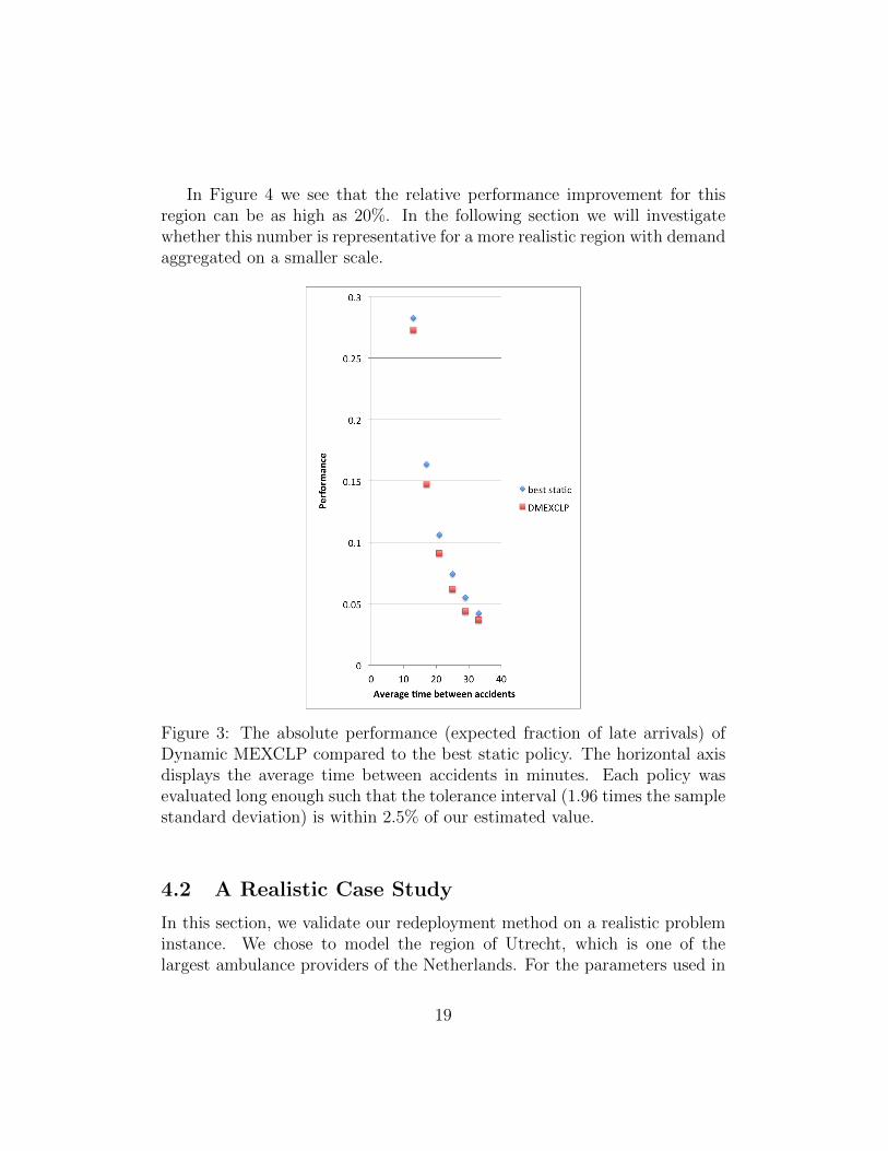
In Figure 4 we see that the relative performance improvement for thisregion can be as high as 20%. In the following section we will investigatewhether this number is representative for a more realistic region with demandaggregated on a smaller scale.

Figure 3: The absolute performance (expected fraction of late arrivals) ofDynamic MEXCLP compared to the best static policy. The horizontal axisdisplays the average time between accidents in minutes. Each policy wasevaluated long enough such that the tolerance interval (1.96 times the samplestandard deviation) is within 2.5% of our estimated value.

4.2 A Realistic Case Study

In this section, we validate our redeployment method on a realistic probleminstance. We chose to model the region of Utrecht, which is one of thelargest ambulance providers of the Netherlands. For the parameters used in

19

Figure 4: The relative improvement in performance of Dynamic MEXCLPcompared to the best static policy. The horizontal axis displays the averagetime between accidents in minutes. Each policy was evaluated long enoughsuch that the tolerance interval (1.96 times the sample standard deviation)of both policies is within 2.5% of the estimated value.

the implementation, see Table 3. This is a region with multiple hospitals,and for simplicity we assume that the patient is always transported to thenearest hospital, if necessary.

Note that we use the fraction of inhabitants as our choice for di. In reality,the fraction of demand could differ from the fraction of inhabitants. However,the number of inhabitants are known with great accuracy, and this is astraightforward way to obtain a realistic setting. Furthermore, the analysisof robust optimization for uncertain ambulance demand in [9] indicates thatwe are likely to find good solutions, even if we make mistakes in our estimatesfor di.

In the Netherlands, the time target for the highest priority emergencycalls is 15 minutes. Usually, 3 minutes are reserved for answering the call,therefore we choose to run our simulations with T = 12 minutes. The drivingtimes for EMS vehicles between any two nodes in V were estimated by theDutch National Institute for Public Health and the Environment (RIVM)in 2009. These are driving times with the siren turned on. For ambulancemovements without siren, e.g., when repositioning, we use 0.9 times the speedwith siren. The number of vehicles used in our implementation is such thata good policy gives a performance (expected fraction of late arrivals) of amagnitude that is realistic for practical purposes.

20

parameter magnitude choiceλ 1/9.5 minutes Realistic for urgent calls on a weekday

in this region.A 19 Realistic number to cover demand.W 19 Base locations as existing in 2013.V 217 4 digit postal codes.H 10 The hospitals within the region in 2013,

excluding private clinics.τij Driving times as estimated by the

RIVM.di Fraction of inhabitants as known in

2009.

Table 3: Parameter choices for our implementation of the region of Utrecht.

Results

We compare the performance of the dynamic MEXCLP solution with abenchmark. We let the benchmark be the static MEXCLP solution, whichis generally assumed to give a good static policy (for a comparison of staticmethods, see [18]). Note that the verification of the value of one single pol-icy is not feasible within polynomial time. Therefore, it is not tractable toperform a brute force search over all static policies using 19 base locationsand 19 vehicles. Since there is no alternative known to compute the optimalstatic solution, this means we cannot use the optimal static solution as abenchmark.

In both the static (benchmark) and the dynamic (proposed solution) case,we initialize the locations of the ambulances according to the static MEXCLPsolution. We simulate the EMS system 10 times per policy and compare theresults in Figure 5. We measure the fraction of late arrivals, which decreasedfrom on average 9.5% to 7.9%. This is a difference of 1.6 percentage point,and a decrease of 16.8%. This is a significant improvement that can be madewithout purchasing extra vehicles or increasing the number of crew shifts.Furthermore, this improvement is large in comparison to other results inliterature (e.g., an improvement from 26.7% to 25.8% in [12], which boilsdown to a 3.4% gain).

We would like to emphasize that the dynamic MEXCLP policy does not

21

0.075

0.08

0.085

0.09

0.095

static dynamicpolicy

fra

ctio

n la

te a

rriv

als

Figure 5: Comparing the performance of Dynamic MEXCLP with the staticMEXCLP solution. For both policies a value of q = 0.3 is used. Each policywas evaluated with 10 runs of 500 simulated hours.

only reduce the expected fraction of late arrivals, but also reduces the averageresponse times overall. This can be concluded from Figure 6.

4.3 Sensitivity to the Busy Fraction

We investigate the sensitivity of Algorithm 1 to the parameter q, the busyfraction. In order to do this, we keep the number of vehicles equal to 19,and we also keep the average time between accidents equal to 9.5 minutes.We run the DMEXCLP algorithm for several values of q, and compare theperformance in Figure 7. We conclude that, at least for this particular prob-lem instance, the quality of the solution is very insensitive to the value ofparameter q.

5 Conclusions

In this paper we have developed real-time scalable algorithms for dynamicambulance redeployment with a focus on minimizing the expected fractionof late arrivals. We have introduced a dynamic MEXCLP heuristic (see Al-gorithm 1) that reduces the expected fraction of late arrivals by relatively

22

0 200 400 600 800 10000

0.1

0.2

0.3

0.4

0.5

0.6

0.7

0.8

0.9

1

seconds

cu

mu

lative fra

ction r

esp

on

se tim

es

Empirical CDF

static

dynamic

Figure 6: Response times for dynamic MEXCLP and the static MEXCLPsolution. For both policies a value of q = 0.3 is used. Each policy wasevaluated with 2,500 simulated hours.

16.8% compared to a good static policy. Additionally, the dynamic MEXCLPheuristic also reduces the average response times overall. The heuristic de-pends on the busy fraction, i.e., the fraction of time that an ambulance isunavailable, that needs to be estimated. Our experiments indicate that goodperformance is still obtained, even if there is an error in the estimation ofthe busy fraction.

5.1 Remarks

In terms of applicability, we find it useful to consider whether the DynamicMEXCLP heuristic is still feasible when we relax some of our assumptions.We address the following cases.

Changes During the Day

In practice, EMS systems may deal with characteristics that change over thecourse of a day. This is reflected in changing parameters in our model. We

23

0.07

0.072

0.074

0.076

0.078

0.08

0.082

0.084

0.086

0,1 0.2 0.3 0.4q

fraction late

arr

ivals

Figure 7: Comparing the performance of DMEXCLP for several values of q.The boxes consist of ten runs, in which we simulate 1000 hours, each.

mention a few examples.

• Accident probabilities may shift, for example, an accident is more likelyto occur in an industrial area during office hours.

• Travel times may be longer in rush hour, or may depend on the weather.

Changing parameters over time, such as the examples above, are often diffi-cult to incorporate in a solution. However, in our case, there is no need tocomplicate the algorithm. At any decision epoch, use the parameters thatare relevant for the upcoming period. The choice of the period size maydepend on the EMS region, but for example 30 minutes would be a goodstarting point.

However, we want to point out that emergency services do not alwaysexperience the impact of the time of day on their response velocities. Forexample, empirical evidence shows only a minor impact for fire fighters inNew York [10] and ambulances in Calgary [2]. Furthermore, even if one iscertain that the time of day is relevant for the response velocities, the taskremains to estimate the different velocities accurately. Care has to be taken

24

as to not make mistakes, e.g., due to the data containing only a small numberof trips from i to j in each time segment. At this moment, we do not haveaccess to accurate time dependent travel time estimates, and therefore wedid not implement such a case study.

Stochastic Travel Times

One straightforward way of dealing with stochastic travel times, is to use theexpectations E[τij] in Algorithm 1. Alternatively, we did some additionalsimulations, in which we found good performance when using the 0.8 quantile,i.e., the number Xij such that P [τij ≤ Xij] = 0.8. The performance will ofcourse depend on the exact distribution function chosen, and we suggestsome preliminary experiments to obtain a good strategy.

Staff Satisfaction

Staff members that come from a ‘static’ work environment may be used tohaving their own, fixed home base. Giving up this concept can be difficult.Although our proposed method already limits the relocation moments, extraadjustments can be made to accommodate the staff. For example, a goodcompromise would be the following. Each vehicle (and the correspondingcrew) still has its own, fixed home base. Preferably, we send the vehicleto this home base, but we may choose another base if the expected gain islarge enough. One can measure this by calculating the marginal coveragethat would be obtained if we were to send the vehicle to its own home base,and compare this with the marginal coverage that could be obtained by arelocation. Finally, one might relocate the vehicle if and only if the differencein marginal coverage is greater than a certain threshold.

Rural Regions

As we mentioned in Section 1.2, our algorithm is designed particularly forbusy (urban) areas. For rural regions, however, the same technique maystill be applicable, albeit with some adaptations. A key observation is thatrural regions have a lower accident frequency - which is directly related tothe frequency at which ambulances become idle. This implies that there willbe fewer relocation moments, and therefore we expect performance improve-ments to be smaller. In order to overcome this, we suggest adding some

25

additional relocations4. For example, one could allow a relocation when anew accident arrives. In addition, it is possible to allow two vehicles to re-locate upon completion of an accident. The decision on where to send thevehicles, can still be made using the Dynamic MEXCLP method.

Multiple Targets

In some countries there exist multiple time targets, depending on the ur-gency of the situation. For example, in the Netherlands, the highest priorityaccidents have to be reached within 15 minutes, and the less severe (but stillurgent) accidents have to be reached within 30 minutes. We advise to applythe Dynamic MEXCLP algorithm using the most strict time target. Ournumerical experiments regarding realistic use cases, indicate that this resultsin a policy that also has a good performance for a target of 30 minutes.

Acknowledgements

The authors of this paper would like to thank the Dutch Public Ministry ofHealth (RIVM) for giving access to the travel times for EMS vehicles in theNetherlands. We also thank the editor and the anonymous referee for theiruseful comments. The first author thanks the EMS provider of the regionUtrecht (Ravu), for discussions, and the opportunity to experience severalaspects of the EMS system in practice. This research was financed in partby Technology Foundation STW under contract 11986, which we gratefullyacknowledge.

References

[1] R. Alanis, A. Ingolfsson, and B. Kolfal. A Markov chain model for anEMS system with repositioning. Production and Operations Manage-ment, 22(1):216–231, 2013.

[2] S. Budge, A. Ingolfsson, and D. Zerom. Empirical analysis of ambulancetravel times: The case of Calgary emergency medical services. Manage-ment Science, 56(4):716–723, 2010.

4This will obviously increase the workload for the crew, but we think this is acceptablesince a rural region is typically not very busy.

26

[3] G. Cady. JEMS 200 city survey, JEMS 2001 annual report on EMSoperational & clinical trends in large, urban areas. JEMS: A Journal ofEmergency Medical Serices, 27(2):46–71, 2002.

[4] R.L. Church and C.S. Revelle. The maximal covering location problem.Papers of the Regional Science Association, 32:101–118, 1974.

[5] M.S. Daskin. A maximum expected location model: Formulation, prop-erties and heuristic solution. Transportation Science, 7:48–70, 1983.

[6] M. Gendreau, G. Laporte, and F. Semet. A dynamic model and par-allel tabu search heuristic for real-time ambulance relocation. ParallelComputing, 27:1641–1653, 2001.

[7] J. Goldberg, R. Dietrich, J.M. Chen, and M.G. Mitwasi. Validating andapplying a model for locating emergency medical services in Tucson,AZ. Euro, 34:308–324, 1990.

[8] K. Hogan and C.S. Revelle. Concepts and applications of backupcoverage. Management Science, 34:1434–1444, 1986.

[9] R.B.O. Kerkkamp. Optimising the deployment of emergency medicalservices. Master’s thesis, Delft University of Technology, 2014.

[10] P. Koleskar, W. Walker, and J. Hausner. Determining the relation be-tween fire engine travel times and travel distances in New York City.Operations Research, 23(4):614–627, 1975.

[11] L. Lee, T. Lau, and Y. Ho. Explanation of goal softening in ordinaloptimization. IEEE Transactions on Automatic Control, 44(1):94–99,1999.

[12] M.S. Maxwell, S.G. Henderson, and H. Topaloglu. Tuning approximatedynamic programming policies for ambulance redeployment via directsearch. Stochastic Systems, 9999. To appear.

[13] M.S. Maxwell, M. Restrepo, S.G. Henderson, and H. Topaloglu. Approx-imate dynamic programming for ambulance redeployment. INFORMSJournal on Computing, 22:226–281, 2010.

[14] W. B. Powell. Approximate Dynamic Programming: Solving the Cursesof Dimensionality. John Wiley & Sons, 2011.

27

[15] J.F. Repede and J.J. Bernardo. Developing and validating a decisionsupport system for locating emergency medical vehicles in Louisville,Kentucky. European Journal of Operational Research, 75:567–581, 1994.

[16] Z. Shen, Q.-C. Zhao, and Q.-S. Jia. Quantifying heuristics in the ordinaloptimization framework. Discrete Event Dynamic Systems, 20(4):441–471, 2010.

[17] C. Toregas, R. Swain, C. ReVelle, and L. Bergman. The location of emer-gency service facilities. Operations Research, 19(6):1363–1373, 1971.

[18] P.L. van den Berg, J.T. van Essen, and E.J. Harderwijk. Comparison ofstatic ambulance location models. Under review, 2014.

[19] D.M. Williams. 2008 JEMS 200 city survey: The future is your choice.JEMS: A Journal of Emergency Medical Services, 34(2):36–51, 2009.

[20] Yisong Yue, Lavanya Marla, and Ramayya Krishnan. An efficientsimulation-based approach to ambulance fleet allocation and dynamicredeployment. In AAAI Conference on Artificial Intelligence (AAAI),July 2012.

[21] O. Zhang, A.J. Mason, and A.B. Philpott. Simulation and optimisationfor ambulance logistics and relocation. Presented at the INFORMS 2008Conference, 2008.

28