an econometric analysis on the co-movement of stock market volatility between china ... · pdf...

International Journal of Business and Social Science Vol. 4 No. 14; November 2013

181

An Econometric Analysis on the Co-Movement of Stock Market Volatility between

China and ASEAN-5

Shaharudin Jakpar

Vejayapurni Vejayon

Faculty of Economics and Business Universiti Malaysia Sarawak

94300 Kota Samarahan Sarawak Malaysia

Anita Johari

Khin Than Myint

School of Business Curtin University of Technology Sarawak Campus

CDT 250, 98000 Miri Sarawak Malaysia Abstract

This study aims to examine the co-movement of stock market volatility between China and ASEAN-5 countries from the year 2000 to 2009. This study applies the standard linear GARCH (1, 1) model where these models estimate using monthly price data from year 2000 to 2009 for China, Malaysia, Singapore, Thailand, Indonesia and Philippines. The standard time series econometrics analysis is used which are ADF unit root test, JJ co-integration test, and Granger causality test. The results indicate the co movement of stock market volatility between China and ASEAN-5 have fairly relation among them. The result shows there are two way relations which are bidirectional causality between china and Indonesia; China and Thailand; and China and Singapore. Meanwhile, there have no causality relation between China and Malaysia; and also China and Philippines. Though, it can be concluded that there are relationship between regions in the stock market volatility.

1. Introduction

1.1 Background of the study

Volatility is a statistical measure of dispersion of returns for a given security or market index. Volatility can either be measured by using the standard deviation or variance between returns from the same security or market index. Generally, the security gets more risky when the volatility is getting higher and higher. There are a few researches on co-movement of volatility market of China, Malaysia, Singapore, Indonesia, Myanmar and Thailand. Nishimura and Men (2010), has done a study on the paradox of China’s international stock market co-movement, they had examine on the daily and overnight volatility spillover effects in common stock prices between China and G5 countries. They have done a study on the existence of volatility spillover effects between China and G5 stock markets by using the EGARCH model, the CCF approach and realized volatility. The empirical results reveal some intriguing characteristics of these markets. They found evidence of short-run one-way volatility spillover effects from China to the US, the UK, German and French stock markets. The empirical results suggest that Chinese investors were not rational and China’s stock market entered a speculative bubble period after the second half of 2006.

An earlier study of volatility Co-movement of ASEAN-5 Equity Markets examines on Economic cross-linkages and the increased co-movement of asset prices across international markets is important outcomes as the result of globalization. It concludes that through the various valid economic tests underlying the issue of economic integration, while the stock market volatility indicated that partial Market integration prevails in the pre-crisis, the post crisis period was in fact completely integrated (Oh et.al., April, 2010).

© Center for Promoting Ideas, USA www.ijbssnet.com

182

The study examines the degree and nature of volatility co-movement between the Malaysian stock market with that of US, UK, Hong Kong and Japan, the extent to which movements in the Malaysian stock market can be explained by shocks in the four major markets. The analysis of volatility co-movement between Malaysia and US, UK, Japan and Hong Kong have yielded some encouraging outcomes to be considered by market analyst and investors. From the analysis, Malaysia is the only market in the analysis with a positive returns (positive mean) and low risk (lowest standard deviation). The analysis also proved that the Malaysian market is less vulnerable to external market movements though it is receptive Japan and US.

In a study of “Financial Co-Movement and Correlation” studies on 33 International Stock Market Indices by Evans (2006). He has initially used established co-integration and multivariate GARCH frameworks, and the results suggest correlations with the US have not in general exhibited an upward trend. The main exception to this is the G7 economies, although even here the correlations. There are two results. First, during normal period when volatility (risk) is low the VaR estimates are similar for both portfolio types. Second, when portfolio risk is high, or increasing, then the level of risk experienced by the equally weighted portfolio is greater than the level of risk experienced by the portfolio which has time-varying weights based upon the estimated correlation coefficient, with the exception of one period for the others portfolio.

According to Raju (2004) on stock Market Volatility, an International Comparison examines on Peripatetic stock prices and their volatility, which has now become endemic features of securities markets add to the concern. The growing linkages of national markets in currency, commodity and stock with world markets and existence of common players, have given volatility a new property that of its speedy transmissibility across markets. It shows that daily average return and daily volatility across markets vary over time and space. Their divergences are highly demonstrable. Some countries (US) provide as high as 0.04 percentage return while some of the emerging markets such as Indonesia recorded negative returns of -0.01 percentages.

On the Volatility and Co-movement of U.S. Financial Markets around Macroeconomic News Announcements the short-term anticipation and response of U.S. studies on stock, Treasury, and corporate bond markets to the first release of surprise U.S. macroeconomic information. The analysis of the extent to which prices in financial markets incorporate fundamental information is central to the theoretical and empirical finance literature. The traditional notion of market efficiency requires that new information about asset payoffs should be quickly and fully reflected in asset prices and drive their dynamics. Prior research has examined the links between financial and real variables by studying the effects of the disclosure of macroeconomic information (often without first identifying its surprise content) on stock and bond markets (Brenner, Pasquariello, Subrahmanyam, 2009).

1.2 Problem statement

The issues of stock markets co-movement linkages had been investigated over the time. The Asian crisis started in mid-1997 had affected the currencies, stock markets, and other asset prices of several Southeast Asian economies. Since then, many economists are concerned about the relationship between Asian stock markets and others in the world. After the Mexican peso crisis in 1994, Western investors have lost confidence in securities in Southeast Asia. Therefore, they began to pull money out, and this situation created a domino effect.

In mid 1997, Thailand was hit by currency speculators, resulting in great damages in the financial sectors of country. What at first appeared to be local financial crisis in Thailand has escalated into a global financial crisis within few months. This spreads to other Asian countries such as Indonesia, Singapore, Malaysia and the Philippines. Then, the Asian crisis turned out to be far more serious than its two predecessors in terms of the extent of contagion and the severity of resultant economic and social costs. Financial institutions and corporations with high foreign currencies debts in the afflicted countries were driven to financial distress and many were forced to default because of the massive depreciations in local currencies.

Several factors were responsible for the onset of Asian financial crisis which are a weak domestic financial system, free international capital flows, the contagion effects of changing market sentiment and inconsistent economic policies. As Asian developing countries ardently sourcing foreign capitals from US, Japanese and European investors, who were attracted to these fast growing emerging markets for extra returns for their portfolios. Large inflows of private capital resulted in a credit boom in the Asian countries in the early and mid-1990s. The credit boom was often directed to speculations in real estate and stock markets as well as to investments in marginal industrial projects.


183

Fixed or stable exchange rates also encouraged un-hedged financial transactions and excessive risk-taking by both lenders and borrowers, who were not much concerned with exchange risk.

As asset prices declined such Thailand, due to the government’s effort to control the overheated economy, the quality of banks’ loan portfolios also declined as the same assets were held as collateral for the loans. In addition, their lending decisions were often influenced by political considerations, likely leading suboptimal allocation of resources. However, the so-called crony capitalism was not a new condition, and the East Asian economies achieved an economic miracle under the same system.

Meanwhile, the booming economies with a fixed or stable nominal exchange rate inevitably brought about an appreciation of the currencies. This, in turn, resulted in a market slowdown in export growth in these Asian countries like Thailand and Malaysia. If the Asian currencies had been allowed to depreciate in real terms which were not possible because of the fixed nominal exchange rates, discrete changes of the exchange rates as observed in 1997 might have been avoided.

There are several reasons that are important for the stock market co-movement to work together. For example, the increase in capital flows across national boundaries and potential benefits from diversification of investment on international level. It is important for the investors to diversify international portfolio if they have the knowledge on the structure of equity market linkages across countries.

This study is to investigate on China and ASEAN-5 namely Malaysia, Singapore, Indonesia, Thailand and Philippines countries whether these countries can be integrated in their movement of stock market with each other due to their economic as trading partners and in terms of investment flows. It is because it is important for these countries to be independent and do not depend on other country such as US so that they can manage when there are crisis happen again as before. So, if the crisis happens again, these countries could manage and it will never impact those countries badly.

In addition, nowadays, the financial markets are getting better capital movements, financial reforms, and advances in computer technology and information processing. These factors have increases the ability to react promptly to news and shocks originating from the rest of the world. This indicates that the linkages between stock markets around the world have grown stronger. Hence there is a need to study these linkages and investigated empirically.

1.3 Objective of the study

1.3.1 General Objective

To determine the co-movement of stock market volatility between China and ASEAN-5 countries from the year 2000 to 2009.

1.3.2 Specific Objective

To investigate the long run relationship of the stock market volatility between China with ASEAN-5 countries.

To investigate the causal direction of the stock market volatility between China with ASEAN-5 countries.

1.4 Significant of study

1.4.1 Existing investors

To all investor of every country whether they are being categorized as retail or institutional investors, the problem in forecasting in the volatility stock market have become one of the major factor that contributing to the lower return from their investment. This phenomenon happens because of their lacking in information regarding to the changes in the economic variables. Due to this, most of them are not able to grasp the opportunities and cannot avoid or reduced the risks because there are changes in stock market variables. Generally, by having this study, the investor might use it as a guideline to predict the future movement of stock market price and consumer price market in the stock market volatility.

1.4.2 Prospect Investors

This study will also contribute to new or prospect investors. Surely they need information regarding the volatility of stock market. They can use it as a consideration as market risk in investment.


184

The investors cannot eliminate it but they can use of it in formulating their strategies in order to diversify the risks. By having information in this study, they will feel more confident in committing themselves in stock market investment. Therefore, the total capital market of the country will increase by having a strong support from new investor who is fully with the knowledge of stock market.

1.4.3 Nation leaders and other researchers

The possible constructive finding may deliver pragmatic evidence with comprehensive features and knowledge to nation leaders, economists and people. Another contribution of work in this research is by employing more advance and specific variables with higher frequency dataset to obtain specific and accurate findings together extra significance measures. However, if the results show weak evidence, then other researches should carry out to develop new techniques to the interdependence and spillover effect.

1.5 Scope of study

On this study of co-movement of stock market volatility between China and ASEAN-5 countries which is Malaysia, Singapore, Philipines, Indonesia and Thailand. The time frame is from 2000 to 2009.

2. Literature Review

2.1 Concept of Co-movement

According Baur (2003), the author of the article of what is Co-Movement, extracts co-movement as: “The movements of assets that is shared by all assets at time”. (p.5)

The author studied on co-movement argues on the term co-movement is used inflationary and that the correlation coefficient is not a natural measure of co-movement. The multinomial logit model used to estimate the co-movement as an alternative of Multivariate GARCH models. The finding shows that the co-movement always increases in crisis periods. Baur stressed out that that it could be condensed to the fact that the co-movement has increased or all ’portfolios’ of markets analyzed and that negative co-movement is generally less probable than positive co-movement. So, it does not mean that negative co-movement is less pronounced than positive co-movement.

Volatility is one of remarkable phenomena in financial market. According to Kiseok, (1988), it signify the underlying process of variability or uncertainty of a transaction or portfolio and is widely used as a measure of risk that financial asset returns. Volatility has a crucial role in theoretical and empirical finance where the trade-off between risk and return is the most fundamental theory. Together with return, risk is used to measure the performance of the portfolio. As investors require higher returns for investing in investment with higher risk, then the fluctuations in price is characteristic of volatility.

One of the most common and basic measure of volatility is called standard deviation, where volatility is measured in relation to a defined time frame. It takes into account the way a security has performed in the past and estimates the probability as whether it will perform in the same manner in the future (Chia, 2003). Generally, the higher the standard deviation, the more volatile is the security.

Meanwhile, according to Vannerson and Rudderow, (2000), another study of measure on risk is the beta coefficient, which measures the volatility of a security in relation to that of the stock market as a whole. Any security with a beta higher than one is more volatile relative to market index and inversely, a beta less than one will yield less volatile than the index. Beta is useful in providing a measurement of a security’s past volatility relative to a specific benchmark or index.

2.2 Review on the co-movement of stock market volatility in emerging stock market

According to Beine and Candelon (2007) in a study of liberalization and stock market co-movement between emerging markets, they investigate the impact of trade and financial liberalization on the degree of stock market co-movement among emerging economies. Multivariate GARCH models are used in this study. Daily data on stock returns of the various national stock markets in order to compute annual estimate of the cross-country correlation are used. Their findings shows it’s strong to alternative measures of capital openness where in estimation technique and to the choice of the measure of stock price co-movements. The result shows that that policy reforms affecting both the real side and the financial system in emerging economies exert strong effects on the behavior of financial investor.


185

Ramlall (2009) has proved that the US subprime crisis has not even spared developing stock market such as SEMDEX in terms of pronounced co-movements with international stock. Symmetric GARCH and asymmetric GJR models were employed. Results show that GARCH model is able to fit in for all the stock markets with the exception of SEMDEX. He found that findings show that volatility clustering has risen on the back of a higher level of unconditional variance noted in the post crisis period. In case of leverage effects, a general rise is noted in the post crisis period.

According to Modi (2008), there are various alternative techniques for recognizing co-movement resulting among the selected developed stock markets and the emerging stock markets of the world. The authors examine the stock market indices of India (SENSEX), Hong Kong (HANGSENG), Mexico (MXX), Russia (RTS), Brazil (BVSP), UK (FTSE-100) and US (DJIA and NASDAQ). Three descriptive tests was done where, they have found all the markets showed positive average daily returns for the selected period. The correlation analysis reveals that there is high correlation between some pairs and low correlation between some market pairs and finally the rolling correlation analysis results indicate that there is considerable volatility in the correlations between the eight stock markets over time. BSE has the positive trend of rolling correlation with other stock indices.

Another study by Wai and Cheung (2000) was done on the impulse of stock market volatility and the market crash of October 1987. They explores on issue of stock returns' volatility spillover from the US stock market to the stock markets of Australia, Hong Kong, Japan, Singapore, and the United Kingdom before, around, and after the October 1987 crash. The unconstrained vector autoregressive (VAR) model was used where the result shows that the crash originated in the US and caused a spillover to other stock markets. The empirical result shows that there is a co-movement between US stock volatility and other stock markets' volatility after the crash.

2.3 Review on previous study of Co-movement of stock market volatility

Le and Vietinbank (2010) have investigated the transmission of mean return and volatility from the US, Japan, and China to the Indonesian and Malaysian markets, using daily data from January 2005 to December 2007. These emerging countries have increased their economic integration in recent years, and their stock markets have achieved remarkable development. Through GARCH model, the authors construct mean return and volatility spillover models to discuss whether regional (China and Japan) and global (the US) impacts are crucial for the determination of stock returns in Indonesia and Malaysia. They found that the US market influences the Indonesian and Malaysian markets. The results also support significant feedback relationships in mean return between Japan and Indonesia and between Japan and Malaysia.

According to Batra and March (2004) on their study on stock return volatility patterns in India, they examines if there has been an increase in volatility persistence in the Indian stock market on account of the process of financial liberalization in India. Asymmetric GARCH model has been used to estimate the element of time variation in volatility. The result shows that liberalization of the stock market or the FII entry in particular does not have any direct implications for the stock return volatility.

Adrian and Rosenberg (2008) have conducted a study on stock returns and volatility. They explores on cross-sectional pricing of volatility risk by decomposing equity market volatility into short- and long-run components. In their study, they used exponential generalized autoregressive conditional heteroskedasticity (EGARCH) model of Nelson (1991), the generalized autoregressive conditional heteroskedasticity components (GARCH components) model of Engle and Lee (1999), and the GARCH-GJR model of Glosten, Jagannathan, and Runkle (1993). In each alternative specification, they include the market variance in the expected return equation. They found that prices of risk are negative and significant for both volatility components, indicating that investors require compensation in order to hold assets that depreciate when volatility rises, even if the volatility shocks have little persistence.

In addition, Brenner, Pasquariello, and Subrahmanyam (2009) had done a study on the short-term anticipation and response of U.S. stock, Treasury, and corporate bond markets to the first release of surprise U.S. macroeconomic information. Authors used estimating several extensions of the parsimonious multivariate GARCH-DCC model of Engle (2002) for the excess holding-period returns on seven portfolios of asset classes. From the study they found that the arrival of surprise macroeconomic news has a statistically and economically significant impact on the U.S. financial markets, but also that this impact varies greatly across asset classes. Mishra and Rahmanthe (2010) studies on the dynamics of stock market return volatility of India and Japan. They used TGARCH-M model where the results shows the stock markets returns data of India and Japan are non-normal and stationary.


186

The stock market return of India is more predictable based on the lagged-realized rates of return than those of Japan. They found that India's stock market is influenced more by positive news and Japan's stock market is influenced more by negative news. In addition, there is also evidence of volatility persistence in both markets.

According to a study by Sarkar and Barat (2003), on the Daily Close Price Index of Bombay Stock Exchange (BSE) that the returns of daily close price index of BSE follow Levy stable distribution and exhibit randomness. The Finite Variance Scaling Method (FVSM) and Diffusion Entropy Analysis (DEA) were used in this study to detect the exact scaling behavior of the daily close price index of the BSE.

According to Chen, Lung, and Wang (2009) on their study on Stock Market Mispricing in Money Illusion or Resale Option, they examine on two hypotheses to explain the mispricing phenomenon which are the money illusion hypothesis (Modigliani and Cohn (1979) and the resale option hypothesis by Scheinkman and Xiong (2003). Their empirical analysis was through two proxies are used for heterogeneous beliefs among investors which are the index share turnover and the implied volatility differential (IVD) between out of the money and at-the-money SPX put options. Their result shows that the level of mispricing is positively related to both share turnover and IVD, and negatively related to expected inflation. They found that a strong resale option effect in stock mispricing underscores the importance of further research in this direction for asset price bubbles.

Another study was done on the investor sentiment spillover effects of the stock index and stock index futures markets of Taiwan. Using GARCH models, this study examines the spillover effects of investor psychology on different trading indices. The results clearly suggest the existence of dynamic relationships between investor sentiment in the spot and futures markets. The empirical findings of the spillover effects of sentiment between the spot market and the futures market may be analyzed in terms of overall implications on market efficiency. The findings clearly reveal that the links between investor sentiment and market returns are only short-term (Wang, 2010).

Bhargava and Konku examine on the impact of elimination of uptick rule on stock market volatility. In this study four different methods to measure volatility are used which are two each for the intraday and daily volatility. Intraday volatility is measured by the method proposed by Parkinson (1980), which uses the daily high and low prices and the method developed by Garman and Klass (1980), which uses the high, low, open, and close price to determine intraday volatility. In addition, daily historical volatility as well the daily conditional variance using GARCH modeling is used for inter-day volatility. DJIA and S&P 500 index are used to determine the impact on volatility of the overall market in response to the elimination of uptick rule. It is found that for both periods the volatility goes up for both the indexes and all the Dow companies irrespective of the method used for measuring volatility. (Bhargava, 2009)

Hong Xie and Jian Li (2010) examine on intraday volatility analysis on S&P 500 stock index future. Modes used are the GARCH series which including GARCH (1,1), EGARCH and IGARCH, moreover run such models again by GARCH-In-Mean process. The result shows that EGARCH model is the best one of intraday volatility estimation in evidence of S&P500 stock index future market. Meanwhile the IGARCH Model is the better one in in-the-sample estimation. Otherwise the IGARCH model is the preferred for estimation in out-of sample and EGARCH model is the better one. GARCH (1,1) model haven’t good performance in the testing. They found that the crucial factor of high frequency trading successful is that accurate forecast the volatility of asset.

Schornick (2009) has done a study on International Capital Constraints and Stock Market Dynamics. The author analyzed two-country situation where separate restrictions on international capital flows interact to affect stock market dynamics, specifically market volatility and correlation. While found that removing either one of the constraints individually can be seen as an event of ‘partial liberalization’, the effects of removing capital outflow restrictions is indeed opposite to those of removing capital inflow restrictions. When multiple constraints are lifted simultaneously, the net effect on stock dynamics will be dominated by the more severely binding of the constraints.

A study on Modeling and Estimation of Volatility in the Indian Stock Market was done by Goudarzi and Ramanarayanan (2010). They attempted to study the volatility and its stylized facts in the Indian stock market. The BSE500 index of Mumbai stock exchange is used as a proxy for the Indian market. In this study, the empirical results shows that GARCH (1, 1) model can adequately describe the BSE500 stylized facts. The results suggest that the volatility in the Indian stock market exhibits the persistence of volatility and mean reverting behavior. Their findings shows that the conditional volatility of the BSE500 was to be quite persistence.


187

Xing, Zhang, and Zhao (2010) investigate whether the shape of the volatility smirk contains relevant information for the underlying stock’s future returns. The results are consistent with the notion that informed traders with negative news prefer to trade out-of-the-money put options, and that the equity market is slow in incorporating the information embedded in volatility smirks. In other words, empirically, the result shows that the majority of individual stock options exhibit a downward sloping volatility smirk pattern. They found that volatility skew has significant predictive power for future cross-sectional equity returns.

Reexaminations of the causes of time varying stock return volatilities study was done by Zhang (2010). He compares fundamentals-based theories with trading volume-based theories. The results have implications for many asset pricing and corporate finance issues. The author found that the concern for investors who cannot fully diversify their investments that investment performance would continually deteriorate, produce by the Campbell et al. (2001) finding, is unwarranted. Next, he found that for large investors, such as mutual funds and pension funds, diversification gains exist mostly in stocks that have high earnings volatilities and high market to book ratios, which, to some extent, are predictable and therefore can be taken into consideration in forming dynamically optimal portfolios. Finally, he found that the empirical facts documented in this paper should help to resolve the theoretical and empirical issues on the cross-sectional relationship between expected returns and idiosyncratic volatilities.

Engsted and Tanggraad (2002) had done a study on the co-movement of US and UK stock markets. According to them the co-movement of US and UK are highly correlated across country. The main empirical findings in is the future excess return in the main determinants of stock market volatility in both the US and UK. Vector auto-regression (VAR) model are used to determine the underlying forces behind the movements in both the US and UK. An empirical model are computed in this study because of variance decomposition require estimates of infinite horizon expectations. The result of the study shows that the major shocks to economic growth have been common to the US and UK where it induced fluctuations in stock returns in the two countries.

Kallberg and Pasquariello (2003), had investigates one of the most fundamental aspects of aspect pricing, the co-movement of security prices, focusing on the degree to which observed correlations cannot be explained by fundamental factors. The author’s studies on Time-Series and Cross-Sectional Excess Co-movement in Stock Indexes had used the OLS and FGLS procedures. We then use the corresponding estimated residuals to compute the unconditional measures of excess co-movement. Their found that excess co-movement is also consistently significant across all industries over the entire time interval.

According to Forbes and Rigobon (2002), their study on no Contagion, only Interdependence, they explained that the correlation coefficients which are conditional on market volatility. They found that under certain assumptions, it is possible to adjust for this bias. Using this adjustment, there was virtually no increase in unconditional correlation coefficients. For example, during the 1997 Asian crisis, 1994 Mexican devaluation, and 1987 U.S. market crash, there is a high level of market co-movement in all periods, however, they were interdependence.

3. Research Methodology

In this study of stock market volatility between China and 5-ASEAN countries and also between them itself where stock market index will be analyzed. The independent variable is stock market index. The study is to explain that its sense for the country to convergence for each other benefit. In relation to it, the stock market volatility of China and 5-ASEAN countries, the sources of data are obtain by using the data stream published by Thomson data stream on monthly basis for the period of TEN (10) years from the year 2000 to 2009. A standard time series econometric analysis is used. In addition, other tests which are correlation coefficient, unit root tests (ADF unit root tests, Philip-peron test and KPss), Toda-Yamamoto (1995), Granger non causality test, Impulse response function and variance decomposition will be used. The information regarding the stock market price index obtained from the Thomson Data Stream of China and 5 ASEAN countries for past TEN (10) years on monthly bases.

3.1 Theoretical framework

According to Narayan and Smyth (2005), integrated markets will contain information on common stochastic trends. Hereby, market inefficiency exists as market predictability can be enhanced through the information contain in other stock market. Moreover, recent empirical works lie upon the view that co-integration does not necessarily imply anything about efficiency.


188

In addition, according to Masih and Masih, (1999), another important aspects within the context of market integration and interdependence is that assets associate with similar level of risk in different countries should lead to similar level of return. Meanwhile, Wheatly (1988), entailed that even without market integration: asset being diversified internationally could possibly be “mean-variance efficient”.

In the portfolio theory, the integration and stock market interdependence addresses the issue of diversifying assets (Forbes, 1993). Mainly, potential gains from international diversification can be examined through the rate of returns on common stock (Levy and Sarnat, 1970).The rate of return for each country is defined as percentage change in the dollar value of its common stock index as below expression (1):

(1)

Where beholds the dollar value of the country’s stock index and (t) is the rate of return in period t. Besides that, according to Jang and Sul (2002), the return using stock market can be simplified into expression (2) as below:

(2) Where Rt signifies the rate of return at period t and Cit is the stock market index during the same period.

This study applies the standard linear GARCH (1,1) model where these models estimate using monthly price data from year 2000 to 2009 for China, Malaysia, Singapore, Thailand, Indonesia and Philippines. For the model, define the information Ωt of monthly returns to be {rt,rt-g,…,r1}. The jointly estimated GARCH (1,1) model introduced by Bollerslev (1986) is then

r1 = µ + ɛt , ɛt = σt zt and zt i.i.d. (0,1) σt

2 = ω + αɛ2t-1 + βσ2

t-1 (1)

Where σt2 is measurable with respect to Ωt-1 and ω > 0, α >0, β ≥ 0 and α + β < 1, such that the model is covariance-stationary that is first two moments of the unconditional distribution of the return series is time invariant. To estimate the impact of asymmetric effect of shocks on volatility, the above specification is replaced with QGARCH (1,1) model

r1 = µ + ɛt , ɛt = σt zt and zt i.i.d. (0, 1) σt

2 = ω + αɛ2t-1 + βσ2

t-1 + γɛt-1 (2)

The additional term γɛt-1 makes it possible for positive and negative shocks to have different effects on conditional volatility. The condition for covariance-stationary is the same GARCH (1,1).

3.2 Econometric methodology

Mainly, unit root tests are applied to test the order of integration between the countries. Time series unit root tests were used along with unit root tests to study the stationary properties of the data. The co-integration test is conducted to study the long-run relationships among the variables. Finally, the continuation and direction of causality in the short-run and long-run will be assessed by using the Granger Causality test based on VECM framework.

3.2.1 Unit root tests

A test of stationary that has become widely popular over the past several years is the unit root test. Based on Chebbi and Boujelbene, (2008), when the number of observation is low, unit root test have a little power. For this reason, two tests were used to examine the results. The standard ADF and KPSS testing principles have different null hypothesis whereby ADF tests the null of unit root and KPSS tests the null of stationary. The purpose of unit root test is to determine whether the series is consistent with I (1) process with a stochastic trend, or if it is consistent with I (0) process, which means it is stationary, with a deterministic trend. It is essential to examine the stationary of the variables before specification and estimation of co-integration and VAR. Since most of the research were on time series analysis this shows that many macroeconomic time series contain unit roots and non-stationary repressors could be invalidate most of the standard empirical results, a test of stationary is important to set up the specification and estimation of the correct model (Engle and Granger, 1987). The test co-integration among variables that were used in the models needs a test for the presence of unit root for every individual variable based on the auxiliary regression. (3)


189

The ADF auxiliary regression test for the existence of a unit root in yt, specifically the logarithm of all model’s variables at time t. The variables ∆yt-1 expresses the lagged first differences, ut adjusts the serial correlation errors and α, β, δ and y is the parameters to be estimated. The null and alternative hypotheses for a unit root in variable yt are: H0: β = 0, H1: β < 0

The test performed consecutively. First, the ADF test is calculated for the sample period, with and without a deterministic trend. The time trend is included in the auxiliary regression equation if the reported ADF t-statistics shows that the regression is statistically significant. If time trend is not included in the examined variables, then the regression equation will reduce the power of the test. A sufficient number of lagged first differences are included to remove any serial correlation in the residuals.

3.2.2 Multivariate co-integration test

Johansen (1988) and Johansen and Juselius (1990) conveyed the co-integration perceptive in the long-run relationship among the selected variables for the research. Cheung and Ng (1998) distinguished that the Johansen’s procedure is more efficient than the two-step approach by Engle-Granger (1987). Cheung and Lai (1993) and Gonzalo (1994) stated that the Johansen procedures have good large and finite-sample properties. Therefore, in this research, procedure developed by Johansen (1988, 1991) and Johansen and Juselius (1990) were used to conduct the Vector Auto-regression (VAR)-based co-integration test. The model is as follows:

(4)

According to the model above, and are the vector of (P x l) and in the other hand, A is considered as an (P x P) matrix form and the l is considered as the identity matrix form. The purpose of this test is to determine whether the possibility of the selected variables which is non-stationary, to have long-run relationships among these variables or not. According to Granger (1981), co-integration means that the non-stationary variables are integrated in the same order with the residuals stationary. If there is co-integration between two variables, then there is a long-run effect that prevents the two time series from drifting away from each other and there is a force existing to converge into long-run equilibrium.

Johansen’s procedures use two likelihood ratio tests, a trace test and maximum Eigen value test to test the number of co-integrating relationships. Trace Test (5) Maximal Eigen Value Test: λ max ) (6)

By referring to equation (5) and (6), T is the number of observation used for estimation, λi is the ith largest estimated Eigen value and the order of r is determined by using the likelihood ratio (LR) trace test statistic suggested by Johansen (1988). The trace statistic either rejects the null hypothesis of no co-integration among the variables (r = 0) or does not reject the null hypothesis which means there is one co-integrating relationship between the variables (r ≤1) (Dritsakis, 2003).

3.2.3 Granger causality test

The Granger Causality test is used to investigate the causal relationships among the variables which are inflation and stock index price in short-run. By using Granger causality approach, the three possible relationships can be identified. First is the inflation-led stock index price. Second, whether the stock index price which leads to inflation and finally is the bi-directional relationship between inflation and stock index price will be identified. Granger causality test is the appropriate method to determine whether the lags of one variable enter into the equation for another variable (Enders, 1995).

The concept of Granger causality (Granger, 1969) is widely used to study causal effects between time series variables. According to Bohm (2009) in a bivariate case X is said to “Granger cause” Y if and only if Y is better predicted by using the past values of X. In other words, if a variable X Granger causes another variable Y, X can be used to predict Y, or X is a possible cause of Y. Feedback exists between these variables, if Y also Granger causes X. The traditional Granger test can be written as:

(7)


190

Whereby is a constant, p is the lag length, t is time, and t is a disturbance term with mean zero. If time series appear to be non-stationary I (1) processes, the direction of Granger causality may be decided upon standard F-tests in the first differenced VAR framework. The test equation takes the form of:-

(8) In the case of two co-integrating variables, the long-run equilibrium relationship is represented by a Vector error correction model (VECM) as follow:-

(9)

ECT is the co-integrating vector which acts as an error correction term. In this procedure, X Granger causes Y, if either the estimated coefficients on lagged values of X or the estimated coefficient on the lagged value of the error term from the co-integrated regression is statistically significant (and vice versa) (Bohm, 2009).

Granger causality tests the constraint that all lags of the variables do not enter significantly into VAR model specification. This is done by a conventional F test. If co-integration is detected, then the Granger causality must be conducted in Vector Error Correction Model (VECM) to avoid problem of misspecification (Granger, 1988). Or else, the analyses may be conducted as a standard first difference vector autoregressive (VAR) model. VECM is a special case of VAR that imposes co-integration on its variables where it allows us to distinguish between short-run and long-run Granger causality. The relevant error correction terms (ECTs) must be included in the VAR to avoid misspecification and omission of the important constraints (Lau et al., 2008). The existence of a co-integrated relationship in the long-run indicates that the residuals from the co-integration equation can be used as an ECT as follows:

Refer to equation (10) and (11), is the lag operator, α0, δ0, β’s and ø’s are the estimated coefficients, m and n are the optimal lags of the series total energy consumptions (EC) and sectoral outputs refer to (X), ζit’s are serially uncorrelated random error terms while µ1 and µ2 measure a single period responses of the EC (X) to a exit from equilibrium. The error correction terms ECT offers an alternative test of causality (or weak erogeneity of the dependent variable). The coefficients on the ECTs represent how fast deviations from the long-run equilibrium are eliminated from following changes in each variable (Bohm, 2009). The null hypothesis for equation (10) is H0: β2,i = 0 for all i and μ1 = 0. This is to test whether EC Granger causes X1. If the null hypothesis were rejected, it means that EC causes X. Besides, in equation (11), the null hypothesis is H0 : ø2,i = 0 for all i and µ2 = 0 in order to test whether X Granger causes EC2 ( Lau et al.,2008).

4. Results and Findings

The empirical findings of the test utilized would be explained in this chapter reviewing their results and provide an interpretation to each of the finding. To identify the co-movement of stock market volatility between China and ASEAN-5 countries, E-Views are applied in this study. There are three tests have been done which is unit root test, co integration test and granger causality test. The overall empirical illustrations are based on data from Thomson data stream which spans from year 1999 to 2009.

4.1 Empirical results

4.1.1 Augmented Dickey-Fuller Unit Root Test (ADF)

1 The null hypothesis for equation (10) is total energy consumption do not Granger causes sectoral output for every sector. 2 The null hypothesis for equation (11) is sectoral outputs do not Granger causes total energy consumption.


191

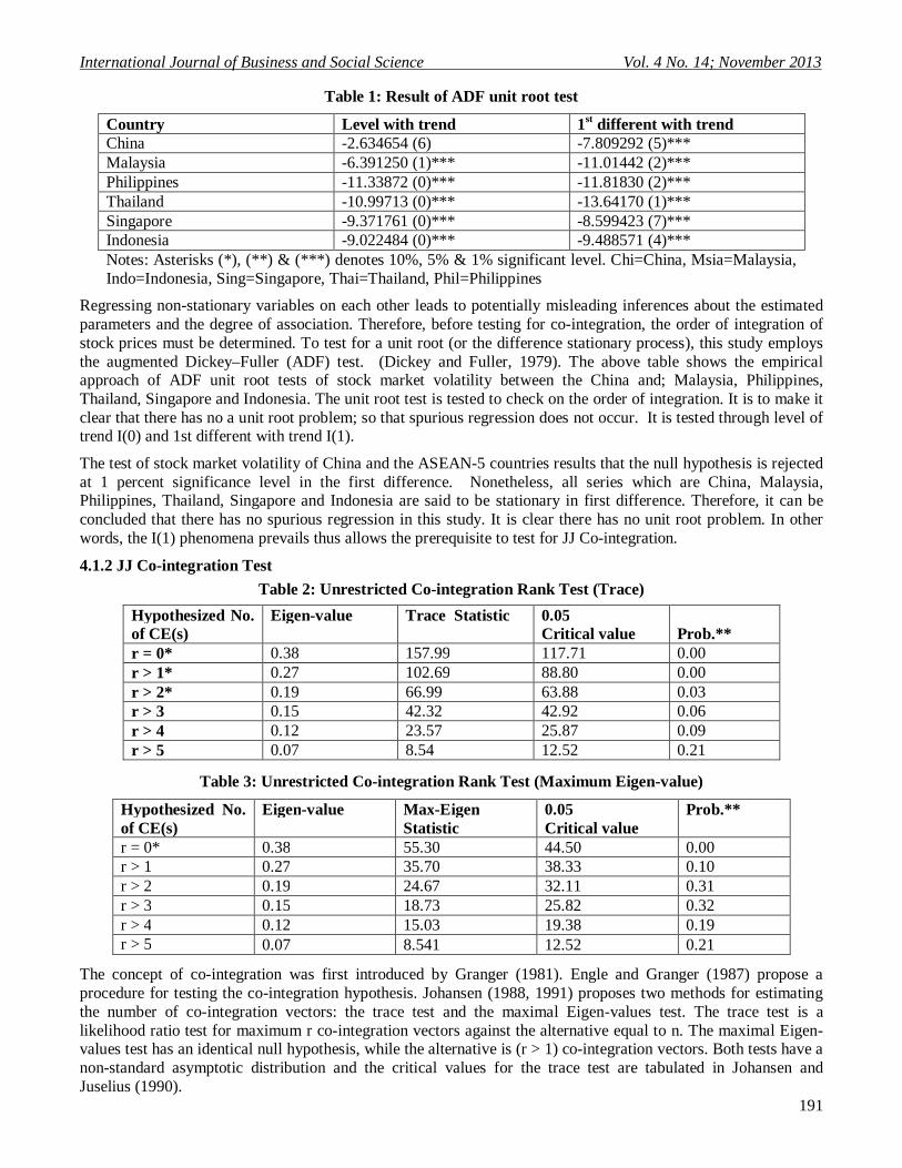
Table 1: Result of ADF unit root test

Country Level with trend 1st different with trend China -2.634654 (6) -7.809292 (5)*** Malaysia -6.391250 (1)*** -11.01442 (2)*** Philippines -11.33872 (0)*** -11.81830 (2)*** Thailand -10.99713 (0)*** -13.64170 (1)*** Singapore -9.371761 (0)*** -8.599423 (7)*** Indonesia -9.022484 (0)*** -9.488571 (4)*** Notes: Asterisks (*), (**) & (***) denotes 10%, 5% & 1% significant level. Chi=China, Msia=Malaysia, Indo=Indonesia, Sing=Singapore, Thai=Thailand, Phil=Philippines

Regressing non-stationary variables on each other leads to potentially misleading inferences about the estimated parameters and the degree of association. Therefore, before testing for co-integration, the order of integration of stock prices must be determined. To test for a unit root (or the difference stationary process), this study employs the augmented Dickey–Fuller (ADF) test. (Dickey and Fuller, 1979). The above table shows the empirical approach of ADF unit root tests of stock market volatility between the China and; Malaysia, Philippines, Thailand, Singapore and Indonesia. The unit root test is tested to check on the order of integration. It is to make it clear that there has no a unit root problem; so that spurious regression does not occur. It is tested through level of trend I(0) and 1st different with trend I(1).

The test of stock market volatility of China and the ASEAN-5 countries results that the null hypothesis is rejected at 1 percent significance level in the first difference. Nonetheless, all series which are China, Malaysia, Philippines, Thailand, Singapore and Indonesia are said to be stationary in first difference. Therefore, it can be concluded that there has no spurious regression in this study. It is clear there has no unit root problem. In other words, the I(1) phenomena prevails thus allows the prerequisite to test for JJ Co-integration.

4.1.2 JJ Co-integration Test

Table 2: Unrestricted Co-integration Rank Test (Trace)

Hypothesized No. of CE(s)

Eigen-value Trace Statistic 0.05 Critical value

Prob.**

r = 0* 0.38 157.99 117.71 0.00 r > 1* 0.27 102.69 88.80 0.00 r > 2* 0.19 66.99 63.88 0.03 r > 3 0.15 42.32 42.92 0.06 r > 4 0.12 23.57 25.87 0.09 r > 5 0.07 8.54 12.52 0.21

Table 3: Unrestricted Co-integration Rank Test (Maximum Eigen-value)

Hypothesized No. of CE(s)

Eigen-value Max-Eigen Statistic

0.05 Critical value

Prob.**

r = 0* 0.38 55.30 44.50 0.00 r > 1 0.27 35.70 38.33 0.10 r > 2 0.19 24.67 32.11 0.31 r > 3 0.15 18.73 25.82 0.32 r > 4 0.12 15.03 19.38 0.19 r > 5 0.07 8.541 12.52 0.21

The concept of co-integration was first introduced by Granger (1981). Engle and Granger (1987) propose a procedure for testing the co-integration hypothesis. Johansen (1988, 1991) proposes two methods for estimating the number of co-integration vectors: the trace test and the maximal Eigen-values test. The trace test is a likelihood ratio test for maximum r co-integration vectors against the alternative equal to n. The maximal Eigen-values test has an identical null hypothesis, while the alternative is (r > 1) co-integration vectors. Both tests have a non-standard asymptotic distribution and the critical values for the trace test are tabulated in Johansen and Juselius (1990).


192

The above tables show the result of the study of co-integration test of stock market volatility and ASEAN-5 countries. As been affirmed before, there are two test of co-integration have been done which are trace test and maximum Eigen-value test. The result of trace test shows there has no long time relationship in stock market volatility between China and ASEAN-5 countries. It is because the result shows they do not move together.

Meanwhile, the result of co-integration on maximum Eigen-value, it shows a good result where there has long run relationship in stock market volatility between China and ASEAN-5. It can be seen in the result that only r = 0 is significant. This means China and ASEAN-5 countries move together in long run relationship. Thus, in this study it is preferable that the result of Eigen-value is more considerable. It is because in co-integration test, the Eigen-values test is more noteworthy than the trace test. According to Chen (2000), the maximal Eigen-values test tends to give better results when the 3trace tests are either large or small. Therefore, for this test of co-integration, this study can conclude that there has long run relationship in stock market volatility between China and ASEAN-5.

4.1.3 Granger causality test Table 4: Result of granger causality test

Null hypothesis F statistics P value Conclusion Indo does not Granger Cause Chi 2.14 0.08* Indo does Granger Cause Chi. Chi does not Granger Cause Indo 4.28 0.00*** Chi does Granger Cause Indo Msia does not Granger Cause Chi 0.75 0.56 Msia does not Granger Cause Chi Chi does not Granger Cause Msia 0.13 0.97 Chi does not Granger Cause Msia Phil does not Granger Cause Chi 0.27 0.90 Phil does not Granger Cause Chi Chi does not Granger Cause Phil 1.00 0.41 Chi does not Granger Cause Phil Sing does not Granger Cause Chi 2.32 0.06* SING does Granger Cause Chi Chi does not Granger Cause Sing 2.72 0.03** Chi does Granger Cause Sing Thai does not Granger Cause Chi 3.69 0.01*** Thai does Granger Cause Chi Chi does not Granger Cause Thai 4.00 0.00*** Chi does Granger Cause Thai Notes: Asterisks (*), (**) & (***) denotes 10%, 5%& 1% significant level. Chi=China, Msia=Malaysia, Indo=Indonesia, Sing=Singapore, Thai=Thailand, Phil=Philippines

The above table shows the granger causality test that results on the null hypothesis of causality on the stock market volatility between China and ASEAN-5 countries. The null hypothesis of causality on the stock market for Indonesia does not granger cause China has been rejected at 10 percent significance level. Therefore, Indonesia seems to granger cause China. Meanwhile, for the examination on stock market volatility for China does not granger-cause Indonesia, the null hypothesis has been rejected at 1 percent significance level. Therefore it is clear that China also granger cause Indonesia.

The null hypothesis of causality on stock market volatility for Malaysia which does not granger-cause China has not been rejected. Otherwise, the null hypothesis of causality on stock market volatility of China does not granger-cause Malaysia also have not been rejected. Therefore, it clarifies that Malaysia and China does not granger-cause each other. The null hypothesis of causality on stock market volatility for Philippines does not granger-cause China have not been rejected. Otherwise, the null hypothesis of causality on stock market volatility of China does not granger-cause Philippines also have not been rejected. Therefore, it also simplifies that Malaysia and China does not dot granger-cause each other.

The null hypothesis of causality on the stock market for Singapore does not granger-cause China has been rejected at 10 percent significance level. Therefore, Singapore seems to granger-cause China. Meanwhile, for the examination on stock market volatility for China does not granger-cause Singapore, the null hypothesis has been rejected at 5 percent significance level. Therefore it is clear that Singapore also granger-cause China.

The null hypothesis of causality on the stock market for Thailand does not granger-cause China has been rejected at 1 percent significance level. Therefore, Thailand seems to granger cause China. Meanwhile, for the examination on stock market volatility for China does not granger-cause Thailand, the null hypothesis has been rejected at 1 percent significance level. Therefore it is clear that China also granger-cause Thailand. As a conclusion, it is clear that there is relationship between China and Indonesia; China and Singapore; and China and Thailand where the null hypothesis have been rejected. Meanwhile, the result also shows that there is no relationship between China and Malaysia; and China and Philippines.


193

5. Discussion

The issues of stock markets co-movement linkages had been investigated over the time. Since the Asian financial crisis in 1997, many economists are concerned about the relationship between Asian stock markets and others in the world. Though, this study examines on the relationship of stock market volatility between China and ASEAN-5 (Malaysia, Indonesia, Thailand, Singapore and Philippines). This study is to examine on the long run relationship of the stock market volatility between China with ASEAN-5 countries.

There are two findings have been found in this study. First, there are long run relationship in stock market volatility between China and ASEAN-5. It shows that China and ASEAN-5 countries move together in long run relationship. The result can be seen it the test of co-integration on maximum Eigen-value where only r = 0 are significance. This shows that the countries move together in a same direction where it means there have relationship in the co-movement of stock market volatility. The second finding is there are relationship in co-movement of stock market volatility between China and Indonesia; China and Singapore; and China and Thailand where the null hypothesis have been rejected in the granger causality test. Meanwhile, the result also shows that there is no relationship between China and Malaysia; and China and Philippines.

The figure 1 below shows the relationship between Malaysia, Indonesia, Singapore, Thailand, Philippines and China.

Figure 1: the co-movement of stock market volatility between China and ASEAN-5

2ways – Bidirectional causality

No causality relation

In the figure 1, summarizes the finding of the study. It shows there are two way relations which are bidirectional causality between china and Indonesia; China and Thailand; and China and Singapore. Meanwhile, there have no causality relation between China and Malaysia; and also China and Philippines. So, it can be concluded that the co movement of stock market volatility between China and ASEAN-5 have fairly relation among them. It is because the findings of the study shows China and three of five countries have two way relationships between them. This shows that the co movement of stock market volatility does have relationship in each other even though this study unable to show there are relation between China and all the five countries.

This study finally has found several policy implications through the various valid economic tests underlying the issue of economic integration. The first policy implication is while the stock market volatility indicated, the partial market are integrated in each other. Second, the formation of Investment Union (IU) for ASEAN-5 is feasible and in fact desirable as market convergence provides one of the many preconditions in establishing a union (with the assessments of other conditional factors to be included as well).

Indonesia

Philippines Malaysia

Singapore

Thailand

China


194

An IU provides a platform for investment funds to flow across borders. Free-flow of capital between borders would discourage saturation of funds within one market as free movement of capital enables the diversion of funds towards less saturated markets. Third, conditionally too, investors may consider another form of investment targeting strategy drawn upon the CI’s volatility through thorough mitigation of the volatility series.

Overall, the securities commission (SC) of each market is responsible to ensure the co-movement of capital markets’ policies and master plan. Witnessing the formation of the ASEAN Investment Area (AIA- 1998) parallel with the establishment of a developed ASEAN Index-Financial Times Stock Exchange (FTSE) regional index are in fact viable initial initiatives to foster regional market convergence.

6. Conclusion and Recommendations

6.0 Introduction

This study was developed in an effort to determine whether there is long run relationship of the stock market volatility between China with ASEAN-5 countries. Further, this study also developed also to identify whether there are causal direction of the stock market volatility between China with ASEAN-5 countries. Last but not least, recommendations and limitations of the research are presented in this chapter, too.

6.1 Limitation of the study

This research focused on the co movement of stock market volatility where it stressed out on the stock index price for 6 countries which are Malaysia, Philippines, Singapore, Thailand, Indonesia and China duration period of year 2000 to 2009. This mean the study only involved in studying the convergence of only six countries where the findings will not represent the overall countries in ASEAN region. So, the linkage uncovered in this study does not hold for other countries thus it does not show the usefulness of the findings if it was to be implement for other countries.

In addition, align to this research, only three test have been discussed in this study which are unit root test, co integration test and, granger causality test while in fact, there are still many other test can be done to identify the co movement of stock market volatility. Moreover, in this study only one variable are used which are stock index price, while there are many other elements that may influence volatility of stock market. Moreover, the study only limited to ten years which are from year 2000 to 2009 because there are some data could not be obtained from the previous years. Other than that, the time frame of covering the field work is also too short. This may limit the researcher to study on more countries and for more long periods.

6.2 Concluding remarks

So far, we have analyzed the co-movement of stock market volatility between China and ASEAN-5 countries from the year 2000-2009. The result of empirical analysis can be summarized that countries are integrated each other in the co-movement of stock market volatility. Therefore it is important for all the country to be concern on the co-movement stock market volatility for precaution of any dilemma. For example, one of the dilemmas that can be seen clearly is in the Asian crisis started in mid-1997 which had affected the currencies, stock markets, and other asset prices of several Southeast Asian economies. However, a single study on this subject is not enough, and further research and studies are required to give more reliable theoretical and empirical proof.

6.3 Recommendations

This paper has provided an overview of the co-movement of stock market volatility. There was fairly relation among countries outcomes highlighted for the overall study. In addition, one shall take note that the data used in this study were only taken from certain and not all countries which are only six countries which are china, Malaysia, Thailand, Malaysia, Philippines, and Singapore. As a result, the findings will not represent the overall countries in this world. Though, in progress of this study, further study must be done. Moreover, throughout this review, this study has attempted to emphasize some of the current literature so as to offer scholars with directions for future research.

Overall, there are numerous opportunities for researchers to further this study based on other element other that stock market such as inflation, interest rate, news announcement and so on. In addition, this study uses panel data analysis where linear examinations are done. So, a non linear study can be used in the further study. Moreover, another recommendation is pool data methodology should be used in further study where it is the best methodology to do an examination.


195

Other that, in further study another test of unit root test can be used which are unit root of structural breaks. Researchers, students, financial professionals, and educators are encouraged to use this paper as a foundation to better understand the existing literature and to identify promising areas for future research. References

Adrian, T., & Rosenberg, J. (2008). Stock Returns and Volatility: Pricing the Short-Run and Long-Run Components of Market Risk. The journal of Finance, Vol.LXIII, No 6.

Batra, A. (2004). Stock return volatility patterns in India. Indian council on International Economic Relations, Working paper 124.

Baur, D. (2003). What is comovement. European Commission, Joint Research Center, Ispra (VA). Beine, M., & Candelon, B. (2007). Liberalization and stock market comovement between emerging markets. Monetary

policy and International Finance. Cesifo Working Paper, No 2131. Bhamra, H.S,. & Uppal, R. (2009). The Effect of Introducing a Non-Redundant Derivative on the Volatility of Stock-

Market Returns When Agents Differ in Risk Aversion. The Review of Financial Studies , v 22 n 6. Bhargava, V., & Konku, D (2010). Impact of elimination of uptick rule on stock market volatility. Journal of Finance

and Accountancy, pg 1-12. Vol 3 July 2010. Böhm, M., Hutchings, M.R. & White, P.C.L. (2009) Contact networks in a wildlife-livestock host community:

identifying high-risk individuals in the transmission of bovine TB among badgers and cattle. PLOSone 4(4): e5016. doi:10.1371/journal.pone.0005016.

Bohm, V., Kaas, L., (2000): Differential savings, factor shares, and endogenous growth cycles," Journal of Economic Dynamics and Control, 24, 965-980

Bohn, Henning, 2009. "Intergenerational risk sharing and fiscal policy," Journal of Monetary Economics, Elsevier, vol. 56(6), pages 805-816, September.

Bollerslev T (1986), Generalized Autoregressive Conditional Heteroskedasticity. Journal of Econometrics,31:307–327. Brenner, M., Pasquariello, P., & Subrahmanyam, M. (2009). On the Volatility and Co movement of U.S. Financial

Markets around Macroeconomic News Announcements. Journal of Financial and Quantitative Analysis, Vol.44, No.6, pp. 1265–1289.

Brenner, M., Pasquariello, P., & Subrahmanyam, M. (2009). On volatility and comovement of U.S. Financial Markets around Macroeconomic News Announcements.

Chebbi H.E and Y.Boujelbene (2008), ‘Agricultural and non-agricultural outputs and energy consumption in Tunisia.;empirical evidences from co-integration and causality ,12 Congress of the European Association of Agricultural Economists (EAAE) .

Chen, C.R., Lung, P.P., & Wang, F.A. (2009). Stock Market Mispricing: Money Illusion or Resale Option. Journal of Financial and Quantitative Analysis, Vol. 44, No. 5, pp. 1125-1147.

Chen, Yongmin, (2000), "Promises, Trust, and Contracts," Journal of Law, Economics and Organization, Oxford University Press, vol. 16(1), pages 209-32, April.

Chen, Yongmin, (2000), "Strategic Bidding by Potential Competitors: Will Monopoly Persist?", Journal of Industrial Economics, Wiley Blackwell, vol. 48(2), pages 161-75, June.

Cheung, Y. W. and Lai, K. S. (1993), Finite-sample Sizes of Johansen's Likelihood Ratio Tests for Cointegration. Oxford Bulletin of Economics and Statistics 55: 313-328.

Cheung, Yin-Wong and Menzie Chinn, 1998, “Integration, Cointegration, and the Forecast Consistency of Structural Exchange Rate Models,” Journal of International Money and Finance 17: 813-830.

Chia, C, K. (2003). Bond Market volatility versus Stock Market Volatility in Malaysia. Unpublished MBA Thesis. Dickey, D. A. and Fuller, W.A. (1979) “Distribution of the estimators for autoregressive time series with a unit root”

Journal of the American Statistical Association, Vol.74, pp. 427–431. Dickey, D.A. and W.A. Fuller (1979), “Distribution of the Estimators for Autoregressive Time Series with a Unit

Root,” Journal of the American Statistical Association, vol. 74, p. 427–431. Dritsakis, N., 2003. Hungarian macroeconomic variables – reflection on causal relationships. Acta Oeconomica, 53:

61-73. Enders, W., 1995. Applied Econometric Time Series. Wiley, New York Engle, R. and Granger, C. W.S. (1987) “Cointegration and error correction: representation estimation and testing”

Econometrica, Vol.55, pp. 251–276. Engle, R. F. and C. W. J. Granger (1987), ACointegration and Error Correction: Representation,Estimation, and

Testing, Econometrica 55, 251-76. Engle, Robert F & Granger, Clive W J, (1987). "Co-integration and Error Correction: Representation, Estimation, and

Testing," Econometrica, Econometric Society, vol. 55(2), pages 251-76, March.


196

Engsted,T., & Tanggaard,C. (2002). The comovement of US and UK stock markets. Centre of Analytic Finance,

Working Paper Series, No. 105. Evan Lau & Koon Po Lee, (2008). "Interdependence of income between China and ASEAN-5 countries," Journal of

Chinese Economic and Foreign Trade Studies, Emerald Group Publishing, vol. 1(2), pages 148-161, December.

Evens, T., & McMillan, D.G. (2006). Financial Co-Movement and Correlation: Evidence from 33 International Stock Market Indices. School of Business & Economics, University of Wales, Swansea.

Forbes, K.J., & Rigobon, R. (2002). No Contagion, Only Interdependence: Measuring Stock Market Comovements. The journal of finance, vol. LVII, no. 5.

Forbes, W.P. (1993), “The integration of European stock markets: The case of the banks”, Journal of Business Finance and Accounting, Vol. 20, pp. 306-686.

Garman, M. B. and Klass, M. J. (1980) On the estimation of security price volatility from historical data ; Journal of Business, 53(1):67--78.

Glosten, Jagannathan, and Runkle (1993) “On the relation between the expected value and the volatility of the Nominal Excess Return on stocks”, The journal of Finance, Vol. XLVIII, No. 5 December 1993

Gonzalo, J. (1994), “Five Alternative Methods of Estimating Long-Run Equilibrium Relationships”, Journal of Econometric, 60, 203-233.

Goudarzi, G., & Ramanarayanan, C.S. (2010). Modeling and Estimation of Volatility in the Indian Stock Market. International Journal of Business and Management, Vol. 5, No. 2.

Granger, C. W. J. (1988) “Some recent development in a concept of causality” Journal of Econometrics, Vol.39, pp. 199–211.

Granger, C. W. J., 1981. "Some properties of time series data and their use in econometric model specification," Journal of Econometrics, Elsevier, vol. 16(1), pages 121-130, May.

Granger, C.W.J. (1969): "Prediction with a Generalized Cost of Error Function," Operational Research Quarterly, 20,199-207.

Granger, C.W.J. (1981). Some properties of time series data and their use in econometric model specification. Journal of Econometrics, 16, 121-130.

Investorwords (2010). The biggest Best Investing Glossary on the Web .Volatility. Retrieved October 31, 2010, from http://www.investorwords.com/5256/volatility.html.

Investorwords (2010). The biggest Best Investing Glossary on the Web. Stock market. Retrieved October 31, 2010, http://www.investorwords.com/4743/stock_market.html.

Jang, H and Sul, W. (2002), “The Asian financial crisis and the co-movement of Asian stock markets”, Journal of Asian Economics, Vol.13, pp. 94-104.

Johansen, S. (1988), A Statistical Analysis of Cointegration Vectors, Journal of Economic Dynamics and Control, 12, 231-54.

Johansen, S. (1991). Estimation and hypothesis testing of cointegration vectors in Gaussian vector autoregressive models. Econometrica, 59, 1551-1580.

Johansen, S. and Juselius, K. (1990) “Maximum Likelihood Estimation and Inference on Cointegration with Applications to the Demand for Money” Oxford Bulletin of Economics and Statistics, Vol.52, pp. 169-210.

Johansen, S., 1991. "A Statistical Analsysis of Cointegration for I(2) Variables," Papers 77, Helsinki - Department of Economics.

Johansen, Soren & Juselius, Katarina, (1990). "Maximum Likelihood Estimation and Inference on Cointegration--With Applications to the Demand for Money," Oxford Bulletin of Economics and Statistics, Department of Economics, University of Oxford, vol. 52(2), pages 169-210, May.

Johansen, Soren, 1988. "Statistical analysis of cointegration vectors," Journal of Economic Dynamics and Control, Elsevier, vol. 12(2-3), pages 231-254.

Kallberg, J., & Pasquariello, P. (2003). Time-Series and Cross-Sectional Excess Comovement in Stock Indexes. Stern School of Business.

Kiseok, N. (1988). Essay on stock market volatility. Unpublished PhD Thesis. Texas A&M University, ATT 9903175. Lau, Chi-Lei Oscar, (2008). "Disentangling Intertemporal Substitution and Risk Aversion under the Expected Utility

Theorem," MPRA Paper 11482, University Library of Munich, Germany. Le, T., & Vietinbank. (2010). International transmission of stock returns: Mean and volatility spillover effects in

Indonesia and Malaysia. The International Journal of Business and Finance Research, Volume 4, Number 1. Lee, Gary, and Robert Engle (1993). "A Permanent and Transitory Component Model of Stock Return Volatility."

Available at SSRN 5848 (1993).


197

Levy, H. and Sarnat, M. (1970), “International diversification of investment portfolios”, American Economic Review,

Vol. 60, pp. 668-675. Masih, A.M.M and Masih, R. (1999), “Are Asian stock market fluctuations due mainly to intra-regional cantogian

effects? Evidence based on Asian emerging stock markets”, Pacific-Basin Finance Journal, Vol. 7, pp. 251-282.

Mishra, B., Rahman, M. (2010). Dynamics of Stock Market Return Volatility: Evidence from the Daily Data of India and Japan. International Business & Economics Research Journal, Volume 9, Number 5.

Modi, A.G., Patel, B.K,. & Patel, N.R. (2010). The Study on Co-Movement of Selected Stock Markets. International Research Journal of Finance and Economics, ISSN 1450-2887 Issue 47.

Modigliani, Franco, and Richard Cohn. 1979. “Inflation, Rational Valuation, and the Market.” Financial Analysts Journal 35(2), pp. 24 - 44.

Narayan, P.K. and Smyth, R. (2005), Cointegration of stock market between New Zealand, Australia and the G7 economies: searching for comovement under structural change, Australian Economic Papers, Vol.44,pp.231-247.

Nelson, Daniel B., (1991). “Conditional Heteroskedasticity in Asset Returns: A New Approach”, Econometrica, Vol.59, No. 2 (Mar, 1991), 347-370

Nishimura, Y., & Men, M. (2010). The paradox of China’s international stock market co-movement: Evidence from volatility spillover effects between China and G5 stock markets. Journal of Chinese Economic and Foreign Trade Studies, Vol. 3 No. 3, 2010, pp. 235-253.

Oh, S.L., Lau, E., Puah, C. H., & Shazali, A.M. (April 2010). Volatility Co-movement of ASEAN-5 Equity Markets. Munich Personal RePEc Archive, MPRA Paper, No. 22244

Parkinson, M.1980. The extreme value method for estimating the variance of the rate of return, Journal of Business, 53(1):61-65.

R. Engle and H. White (ed.) Cointegration, Causality, and Forecasting: A Festschrift in Honor of Clive W. J. Granger, Oxford University Press, pp. 475–497.

Raju, M. T., Ghosh, A. (2004). Stock Market Volatility-An International Comparison. Securities and Exchange Board of India, Working Paper Series No. 8

Ramlall, I. (2010). Has the US Subprime Crisis Accentuated Volatility Clustering and Leverage Effects in Major International Stock Markets. International Research Journal of Finance and Economics, Issue 39.

Sarkar, A., & Barat, (2003). P. Statistical Analysis on Bombay Stock Market. Variable Energy Cyclotron Centre. Scheinkman, Jose, and Wei Xiong, 2003, Overconfidence and speculative bubbles, Journal of Political Economy 111,

1183–1219. Schornick, A.V. (2009). International Capital Constraints and Stock Market Dynamics. INSEAD Working Papers

Collection. Toda, H.Y., & Yamamoto, T. (1995). Statistical inference in vector autoregressive with possibly integrated processes.

Journal of Econometric, 66, 225-250. Vannerson, F.L., Rudderow, T, J. (2000). Effective Asset Allocation. A comparison of Returns and Volatility. Special

report, Futures Investment Series No.1, Mount Lucas Management Corp. Wai, D., & Cheung, W. (2000). The Impulse of Stock Market Volatility and the Market Crash of October 1987. Journal

of Business Finance & Accounting. Wang, Y.M., Li, C.A., & Lin, C.F. (2010). The Investor Sentiment Spillover Effects of the Stock Index and Stock

Index Futures Markets of Taiwan. Northeast Decision Sciences Institute Proceedings, pg 93-98. Wheatly, S. (1988) “Some tests of international equity integration”, Journal of Financial economics, Vol. 21, pp. 177-

212. Xie, H., & Li, J. (2010). Intraday Volatility Analysis on S&P 500 Stock Index Future. International Journal of

Economics and Finance, Vol. 2, No. 2. Xing, Y., Zhang, X., and Zhao, R. (2010). What Does the Individual Option Volatility Smirk Tell Us About Future

Equity Returns? Journal of Financial and Quantitative Analysis, Vol 45, No 3, pp. 641–662. Yongmin Chen, (2000). "On Vertical Mergers and Their Competitive Effects," Econometric Society World Congress

2000 Contributed Papers 0383, Econometric Society. Zhang, C. (2010). A Reexamination of the Causes of Time-Varying Stock Return Volatilities. Journal of financial and

quantitative analysis, Vol. 45, No. 3, pp. 663–684

an econometric analysis on the co-movement of stock market volatility between china ... · pdf...

Documents