four essays on the econometric modelling of volatility and
TRANSCRIPT
Four Essays on the Econometric Modelling
of Volatility and Durations

EFI MissionEFI, the Economic Research Institute at the Stockholm School of Economics, is a scientific institutionthat works independently of economic, political and sectional interests. It conducts theoretical andempirical research in the management and economic sciences, including selected related disciplines.The Institute encourages and assists in the publication and distribution of its research findings and isalso involved in the doctoral education at the Stockholm School of Economics. At EFI, the researchersselect their projects based on the need for theoretical or practical development of a research domain,on their methodological interests, and on the generality of a problem.
Research OrganizationThe research activities at the Institute are organized into 20 Research Centres.Centre Directors are professors at the Stockholm School of Economics.
EFI Research Centre: Centre Director:
Management and Organisation (A) Sven-Erik SjostrandCentre for Entrepreneurship and Business Creation (E) Carin HolmquistPublic Management (F) Nils BrunssonInformation Management (I) Mats LundebergCentre for People and Organization (PMO) Andreas WerrCentre for Innovation and Operations Management (T) Par AhlstrmCentre for Media and Economic Psychology (P) Richard WahlundCentre for Consumer Marketing (CCM) Magnus SoderlundCentre for Information and Communication Research (CIC) Per AnderssonMarketing, Distribution and Industrial Dynamics (D) Bjorn Axelsson
Centre for Strategy and Competitiveness (CSC) Orjan SolvellAccounting and Managerial Finance (B) Johnny LindCentre for Financial Analysis and Managerial Economics in Accounting(BFAC)
Kenth Skogsvik
Finance (FI) Clas BergstromCentre for Health Economics (CHE) Bengt JonssonInternational Economics and Geography (IEG) Mats LundahlEconomics (S) Paul SegerstromEconomic Statistics (ES) Anders WestlundCentre for Business Law (RV) Johnny HerreCentre for Tax Law (SR) Bertil Wiman
Chair of the Board: Professor Carin HolmquistDirector: Associate Professor Filip Wijkstrom
AddressEFI, Box 6501, SE-113 83 Stockholm, Sweden • Website: www.hhs.se/efi/Telephone: +46(0)8-736 90 00 • Fax: +46(0)8-31 62 70 • E-mail [email protected]

Four Essays on the Econometric Modelling
of Volatility and Durations
Cristina Amado

Dissertation for the Degree of Doctor of Philosophy, Ph.D.Stockholm School of Economics 2009.
c© EFI and the author, 2009ISBN 978-91-7258-794-6
Keywords:Financial econometrics; Model specification; Misspecification testing; Nonstationar-ity; GARCH; Unconditional heteroskedasticity; Long financial time series; Ultra-high-frequency data; Diurnal Variation.
Printed by:Elanders, Vallingby 2009
Distributed by:EFI, The Economic Research InstituteStockholm School of EconomicsP O Box 6501, SE 113 83 Stockholm, Swedenwww.hhs.se/efi

To my parents, Arminda e Jose,
for their example
The Road goes ever on and onDown from the door where it began.Now far ahead the Road has gone,And I must follow, if I can,Pursuing it with eager feet,Until it joins some larger wayWhere many paths and errands meet.And whither then? I cannot say.
The Road goes ever on and onOut from the door where it began.Now far ahead the Road has gone,Let others follow it who can!Let them a journey new begin,But I at last with weary feetWill turn towards the lighted inn,My evening-rest and sleep to meet.
J.R.R. Tolkien in “The Lord of the Rings”


Contents
Acknowledgements ix
1 Introduction 1
2 Modelling Conditional and Unconditional Heteroskedasticity withSmoothly Time-Varying Structure 92.1 Introduction . . . . . . . . . . . . . . . . . . . . . . . . . . . . . . . . . 122.2 The model . . . . . . . . . . . . . . . . . . . . . . . . . . . . . . . . . . 132.3 Testing parameter constancy . . . . . . . . . . . . . . . . . . . . . . . 192.4 Model specification . . . . . . . . . . . . . . . . . . . . . . . . . . . . . 252.5 Estimation of the TV-GARCH model . . . . . . . . . . . . . . . . . . 272.6 Misspecification testing of TV-GARCH models . . . . . . . . . . . . . 292.7 Simulation study . . . . . . . . . . . . . . . . . . . . . . . . . . . . . . 382.8 Applications . . . . . . . . . . . . . . . . . . . . . . . . . . . . . . . . . 422.9 Concluding remarks . . . . . . . . . . . . . . . . . . . . . . . . . . . . 48
3 Modelling Changes in the Unconditional Variance of Long StockReturn Series 753.1 Introduction . . . . . . . . . . . . . . . . . . . . . . . . . . . . . . . . . 783.2 A model for the long-term volatility component . . . . . . . . . . . . . 793.3 Estimation of parameters . . . . . . . . . . . . . . . . . . . . . . . . . 833.4 Application to the Dow Jones Industrial Average index . . . . . . . . 853.5 Monte Carlo experiment . . . . . . . . . . . . . . . . . . . . . . . . . . 933.6 Conclusions . . . . . . . . . . . . . . . . . . . . . . . . . . . . . . . . . 96
4 Conditional Correlation Models of Autoregressive Conditional Het-eroskedasticity with Nonstationary GARCH Equations 1074.1 Introduction . . . . . . . . . . . . . . . . . . . . . . . . . . . . . . . . . 1104.2 The model . . . . . . . . . . . . . . . . . . . . . . . . . . . . . . . . . . 1114.3 Estimation of parameters . . . . . . . . . . . . . . . . . . . . . . . . . 1144.4 Modelling with TVGJR-GARCH models . . . . . . . . . . . . . . . . . 1184.5 Empirical analysis . . . . . . . . . . . . . . . . . . . . . . . . . . . . . 1204.6 Conclusions . . . . . . . . . . . . . . . . . . . . . . . . . . . . . . . . . 125
vii

viii Contents
5 A Smooth Transition Approach to Modelling Diurnal Variation inModels of Autoregressive Conditional Duration 1515.1 Introduction . . . . . . . . . . . . . . . . . . . . . . . . . . . . . . . . . 1545.2 The ACD framework . . . . . . . . . . . . . . . . . . . . . . . . . . . . 1555.3 Adjusting diurnal variation with smooth transitions . . . . . . . . . . 1565.4 Specification tests for the diurnal component . . . . . . . . . . . . . . 1575.5 An application to the IBM trade durations . . . . . . . . . . . . . . . 1595.6 Conclusions . . . . . . . . . . . . . . . . . . . . . . . . . . . . . . . . . 164

Acknowledgements
My adventure in Scandinavian lands and frozen seas is finally coming to an end.Many were the frustrating days, sleepless nights, lonely moments and an uncountablenumber of lost weekends during my voyage of discovery in the land of Econometricresearch. The next paragraphs are dedicated to everyone who helped me to see thesunshine in the long dark days during my lonely expedition.
First of all, I would like to express my sincere gratitude to my supervisor, TimoTerasvirta, for his excellent guidance in the rough hills of Nonlinear Time SeriesModels. I am particularly thankful to him for being always available to listen tome, for his invaluable comments and for his tolerance during the teaching semestersI spent in Portugal. His exceptional skills and extraordinary intuition have helpedme so many times to see the light at the end of the tunnel. It has been an absoluteprivilege to learn from and to work with him.
Special thanks go to Sune Karlsson who has given me the opportunity to pursuemy Ph.D. studies at the former Department of Economic Statistics at StockholmSchool of Economics. I also would like to thank Stefan Lundbergh for his guidanceand for his extremely useful advices at an early stage of this thesis. Many thanksto my fellow Ph.D. students and to the faculty at SSE for providing a friendly andstimulating working environment. I am also indebted to Pernilla Watson for helpingme with administrative problems.
This thesis has benefited greatly from the inspiring research atmosphere at CRE-ATES, University of Aarhus, which I had the opportunity to visit twice during theSpring. Very special thanks go to Niels Haldrup for making my visit possible. Bothvisits have been financed by the Louis Fraenckels Stiependiefond.
I also express my gratitude to the direction of the Department of Economics atthe University of Minho for allowing me, in the past three years, to spend the Springsemesters abroad to work on my doctoral thesis.
Many of my thanks go to my dear friend Jana Eklund for her unconditional helpin practical matters surrounding the editing of this thesis. Thank you so much, Jana!I am also extremely grateful to Andres Gonzalez. He has taught me how to code myfirst simulations in Ox programming language when a computer code seemed to mea collection of ancient Egyptian Hieroglyphs.
ix

x
To all my friends I met in Stockholm, I thank you for making my stay more pleas-ant and less lonely. My warmest thanks go to Agatha Murgoci, Ana Beleza, BirgitStrikholm, Helina Laakkonen, Ingvar Strid, Jaewon Kim, Mika Meitz, Milo Bianchi,Mirco Tonin, Rickard Sandberg, Sam Azasu, Tomoaki Nakatani and Zhenfang Zhao.Our social events and nice talks will always be remembered.
Thanks to my friend Ganesh with whom I shared so many happy and not so happymoments in the past years. He has been my office mate, neighbour and my best friendwhen I was in Stockholm. Thank you for your ever-patience, for the funny talks andfor the valuable discussions about the fundamental things in life.
Several colleagues and friends in Portugal also deserve a special mention. Specialthanks go to all my dearest friends from the University of Evora who have alwaysbelieved in me. I really appreciate your loyal friendship and, in my heart, our goodold times will always be remembered as the best moments of my life. I am also verygrateful to Joana Girante and Luıs Aguiar-Conraria for being always there for me andfor their boosting morale. I am thankful to them and to Miguel Portela for helping mein midterm proctoring and grading when I was away. Carla Monteiro and HenriqueCizeron are the best Vets one can have for their pets. Thank you so much for yourfriendship and especially for your patience during the exorcism sessions, days beforemy way back to Stockholm.
Special thanks are dedicated to all my family for their unconditional love and forcheering me on. My dearest aunts, Ivone Silva and Odete Gregorio, have never forgotto call me on the important event dates and have always shown me their supportthroughout these years.
Thanks to my traveller companion, Juno, for making my long working hours duringthe night a little more sweet and for showing me with his meows and purrs that lifeis much more than research.
I especially need to thank Filipe Cizeron for the encouraging words and for beingon the other side of the phone when I most needed. Without his motivation for doingmy doctoral studies abroad it would not be possible to write this dissertation. Thankyou for sharing my joys and for smoothing my way through the troubled times.
Special gratitude goes to my parents for giving me the opportunity to learn despitetheir sacrifice. To my dearest mother, I am deeply thankful for her unconditional loveand encouragement in my most challenging endeavors. To my beloved father, forbeing my source of inspiration, who missed sharing this moment but always has aspecial place in my heart. To them I dedicate this thesis.
Financial support from the Stockholm School of Economics and the University ofMinho is gratefully acknowledged.
Stockholm, May 2009Cristina Amado

Chapter 1
Introduction
1


Introduction 3
This thesis consists of four research chapters in the area of financial econometricson topics of the modelling of financial market volatility and the econometrics of ultra-high-frequency data. The aim of the thesis is to develop new econometric methodsfor modelling and hypothesis testing in these areas. A brief introduction to thoseresearch areas and a short description of the specific topics in the chapters follows.For a more detailed overview of the contents of the chapters, the reader is referred tothe introductions of the individual chapters.
When making investment decisions, volatility is commonly regarded by marketinvestors as a measure of risk. Modelling volatility is therefore essential in manyfinancial areas such as portfolio diversification, risk management, and derivative assetpricing. The models can be then used for forecasting volatility of stock prices, strikeprices or interest rates. The success of the volatility model will depend on how well itpredicts and captures the characteristics of financial data. Financial market volatilityis also of great importance in financial regulation, monetary policy and economicactivity. The central role of risk (or volatility) in financial decision making and theample evidence that the measures of risk exhibit stochastic behaviour through timehave stimulated the development of many sophisticated tools in the field of time serieseconometrics.
The Autoregressive Conditional Heteroskedastic class of models introduced byEngle (1982)1 was designed to parameterize time-varying volatility. The GeneralizedARCH (GARCH) process defined by Bollerslev (1986) specifies present volatility as afunction of past volatilities in addition of past squared returns. The GARCH modelis able to capture the temporal dependence in financial time series by allowing theinvestors to update their risk expectations when new information becomes availableon the market. Moreover, the GARCH model also successfully accommodates somespecial features of financial data such as volatility clustering and excess kurtosis. Sinceits introduction, richer parameterizations and numerous extensions to the GARCHmodel have been suggested to increase the flexibility of the original model.
A vast literature focusing on the implications of the assumption of parameter con-stancy in the GARCH model has been developed in recent years. The occurrence ofsocial, polical or economic events during a long time span may make the structureof volatility to change over time, making the series to become nonstationary. Forthis reason, as Mikosch and Starica (2004) documented, the assumption of station-arity (or parameter constancy) may not be very appropriate when the series to bemodelled is sufficiently long. In applications it is often found that the sum of theestimated GARCH parameters (excluding the intercept) is close to unity. This so-called ‘integrated GARCH effect’ may be well explained by occasional level shifts inthe intercept of the GARCH model; Diebold (1986) and Lamoureux and Lastrapes(1990). This means that the high persistence (or the observed long-memory) in stockmarket volatility may not be an inherent feature of the financial data but it can beexplained by neglected structural breaks in the variance process.
1Robert F. Engle was awarded in 2003 the Sveriges Riksbank Prize in Economic Sciences inMemory of Alfred Nobel “for methods of analyzing economic time series with time-varying volatility(ARCH)”.

4 Chapter 1
Some modelling proposals have been suggested to accommodate deterministicchanges in the volatility. One possibility is to use Markov-switching GARCH-typeprocesses for modelling sudden breaks in the volatility at specific points in time.Alternatively, one may consider that volatility is parameterized by a ’smoothly’ non-stationary process. One of such models is the spline-GARCH of Engle and Gon-zalo Rangel (2008) in which volatility is multiplicatively decomposed into stationaryand nonstationary components. More specifically, the nonstationary component ismodelled using an exponential spline, and the stationary component is described asa GARCH process.
The chapter “Modelling Conditional and Unconditional Heteroskedasticity withSmoothly Time-Varying Structure”2 introduces a new model, the time-varying GARCH(TV-GARCH) model, in which volatility has a smooth time-varying structure of eitheradditive or multiplicative type. To characterize smooth changes in the (un)conditionalvariance we assume that the parameters vary smoothly over time according to thelogistic transition function. As a result, the parameterizations provide very flexi-ble representations of volatility, and they can describe many types of nonstationarybehaviour. These parametric alternatives are particularly useful in applications formodelling long financial data where the non-constancy of parameters becomes an is-sue. Testing parameter constancy is therefore an important tool for checking theadequacy of the model. For this reason, we provide a modelling framework relying onstatistical inference to specify the parametric structure of the TV-GARCH models.We first test the standard GARCH model against these time-varying alternatives and,in case of the rejection of the null hypothesis, determine the structure of the time-varying component is from the data. This is done by testing a sequence of hypothesesby Lagrange multiplier tests presented in the chapter. Misspecification tests are alsoprovided for evaluating the adequacy of the estimated model.
Finite-sample properties of the test statistics and sequential testing are examinedby simulation. The Monte Carlo experiments suggest that these procedures havereasonable good properties already in samples of moderate size. The model buildingstrategy is illustrated with an application to the daily S&P 500 index and the spotSPD/USD exchange rate returns. The results show that the tests strongly rejectthe hypothesis of parameter constancy against the time-varying GARCH alternativesfor the two return series. Moreover, our findings suggest that the long-memory typebehaviour of the sample autocorrelation functions of the absolute or squared returnscan also be explained by deterministic changes in the unconditional variance.
In some applications, the time series used for fitting a GARCH model coversdecades of economic activity. For such long series, one may inevitably expect periodsof turbulence such as recessions and, possibly, deterministic shifts. In those cases,the assumption of constant unconditional variance of the GARCH model turns outto be too restrictive. Shifts in the unconditional variance then affect the estimationtowards an IGARCH model as documented in Lamoureux and Lastrapes (1990).
2This is a joint work with Timo Terasvirta.

Introduction 5
Consequently, modelling deterministic changes in the second unconditional momentof the returns is important when the time series covers a long period.
The chapter “Modelling Changes in the Unconditional Variance of Long StockReturn Series”3 addresses the issue of modelling deterministic changes in the uncon-ditional variance over a long return series. For this purpose, we assume that volatilityis modelled by a multiplicative decomposition of both conditional and unconditionalvariance. More specifically, the conditional variance component is parameterized bya GARCH-type model and it describes the short-run dynamics. The unconditionalvariance component is assumed to be vary slowly over time and it is modelled using alinear combination of logistic transition functions. The structure of the time-varyingcomponent is specified using a testing sequence which is similar to the one withinthe TV-GARCH framework. In order to facilitate the specification, the long series issplitted into non-overlapping subperiods, and parameter estimation in this modellingframework requires special care. The modelling strategy is illustrated with an appli-cation to the daily returns of the Dow Jones Industrial Average (DJIA) index from1920 until 2003. The empirical results sustain the hypothesis that the assumptionof constancy of the unconditional variance is not adequate over long return seriesand indicate that deterministic changes in the unconditional variance may be associ-ated with macroeconomic factors. The observed long-memory property observed inthe original series is weakened when the deterministic changes in the unconditionalvariance are incorporated into the model.
Many financial considerations do not only rely on the behaviour of an individualasset. Instead, standard tools applied by financial analysts typically use informa-tion about the covariances or correlations between asset returns. This has moti-vated the modelling of volatility using multivariate financial time series rather thanmodelling individual returns separately. However, the growing literature on multi-variate GARCH models has so far paid little attention on modelling multivariatefinancial data with nonstationary volatilities. Recently, Hafner and Linton (2008)proposed a semiparametric generalization of the spline-GARCH model of Engle andGonzalo Rangel (2008) in which the parametric component is a first-order BEKKmodel. The authors suggested an estimation procedure for the parametric and non-parametric components and established semiparametric efficiency of their estimators.
In the chapter “Conditional Correlation Models of Autoregressive ConditionalHeteroskedasticity with Nonstationary GARCH Equations”4 we propose an extensionof the univariate multiplicative TV-GARCH model to the multivariate ConditionalCorrelation GARCH (CC-GARCH) framework. The variance equations are parame-terized such that they combine the long-run and the short-run dynamic behaviour ofthe volatilities. In this framework, the long-run behaviour is described by the individ-ual unconditional variances, and it is allowed to vary smoothly over time accordingto the logistic transition function. Our model differs from the semiparametric modelof Hafner and Linton (2008) in the sense that a data-based modelling technique is
3This is a joint work with Timo Terasvirta.4This is a joint work with Timo Terasvirta.

6 Chapter 1
used for specifying the deterministic time-varying component. It may be of interest toinvestigate how careful specification of the individual variances affects the correlationstructure of several CC-GARCH models. The effects of modelling the nonstationaryvariance component are examined empirically using pairs of seven daily stock returnseries from the S&P 500 index. According to the results, the nature and magnitudeof the effects on the correlation estimates depend on the correlation structure matrixof the model. The fit of the CC-GARCH models to the data is remarkably improvedthrough taking nonstationarity in variances into account. Another advantage of thisframework is that we are able to generalize the news impact surfaces of Kroner andNg (1998) such that they can vary over time. The so-called time-varying news impactsurfaces are now able to distinguish between responses at different levels of turbulencein the market as well as at different correlation levels.
With the increasing availability of intraday databases, new methods in time serieseconometrics are needed to investigate the recorded information of these more de-tailed and complex datasets. The available information usually contains the precisetime (“time-stamp”) at which the order in the stock market has been executed andother associated characteristics with the trade. Transaction data containing recordedfinancial events at the highest frequency possible are defined as ultra-high-frequencydata. An inherent feature of such data is that the events are irregularly spaced.Standard tools of time series econometrics are thus inadequate for such time seriesas they are based on regularly spaced data. This has contributed to the birth of anew branch of financial econometrics where the so-called high-frequency models havebeen introduced to account the irregular spacing of the data.
The pioneering work on this area was originated with the class of AutoregressiveConditional Duration (ACD) models of Engle and Russell (1998) and Engle (2000).The focus in this work was on modelling the time elapsed between two market events(or duration). Duration data share some of the stylized facts present in financial datasuch as duration clustering, high persistence and, among others, fat tails. Anotherdocumented feature of the data is their systematic pattern over the day as tradingactivity tends to be more active near the opening and closing of the market thanin the midday. In the chapter “A Smooth Transition Approach to Modelling Diur-nal Variation in Models of Autoregressive Conditional Duration”5 we propose a newparameterization for describing the diurnal component. This is done by allowingthe durations to change smoothly over the day according to the logistic transitionfunction. For the purpose, we provide a modelling framework for specifying the pa-rameteric structure of the systematic pattern over the trading day. An application tothe IBM trade durations suggests that the diurnal pattern may not always have theshape proposed earlier: short durations early and late in the day and lower activityin the middle. For this reason, one should proceed with care when specifying thediurnal component. The estimation of the ACD model should be then preceded by aspecification search to determine the structure of the diurnal variation.
5This is a joint work with Timo Terasvirta.

Bibliography
Bollerslev, T. (1986): “Generalized Autoregressive Conditional Heteroskedastic-ity,” Journal of Econometrics, 31, 307–327.
Diebold, F. X. (1986): “Comment on ”Modelling the Persistence of ConditionalVariance”, by R. Engle and T. Bollerslev,” Econometric Reviews, 5, 51–56.
Engle, R. F. (1982): “Autoregressive Conditional Heteroskedasticity with Estimatesof the Variance of United Kingdom Inflation,” Econometrica, 50, 987–1007.
Engle, R. F. (2000): “The Econometrics of Ultra-High-Frequency Data,” Econo-metrica, 68, 1–22.
Engle, R. F., and J. Gonzalo Rangel (2008): “The Spline-GARCH Model forLow-Frequency Volatility and its Global Macroeconomic Causes,” Review of Fi-nancial Studies, 21, 1187–1222.
Engle, R. F., and J. R. Russell (1998): “Autoregressive Conditional Duration: ANew Model for Irregularly Spaced Transition Data,” Econometrica, 66, 1127–1162.
Hafner, C., and O. Linton (2008): “Efficient Estimation of a Multivariate Multi-plicative Model,” Unpublished paper.
Kroner, K. F., and V. K. Ng (1998): “Modeling Asymmetric Comovements ofAsset Returns,” Review of Financial Studies, 11, 817–844.
Lamoureux, C. G., and W. D. Lastrapes (1990): “Persistence in Variance, Struc-tural Change, and the GARCH Model,” Journal of Business & Economic Statistics,8, 225–234.
Mikosch, T., and C. Starica (2004): “Nonstationarities in Financial Time Series,the Long-Range Dependence, and the IGARCH Effects,” The Review of Economicsand Statistics, 86, 378–390.
7


Chapter 2
Modelling Conditional andUnconditionalHeteroskedasticity withSmoothly Time-VaryingStructure
9


11
Modelling Conditional and Unconditional
Heteroskedasticity with Smoothly Time-Varying
Structure 1
Abstract
In this paper, we propose two parametric alternatives to the standard GARCH model.They allow the conditional variance to have a smooth time-varying structure of eitheradditive or multiplicative type. The suggested parameterizations describe both non-linearity and structural change in the conditional and unconditional variances wherethe transition between regimes over time is smooth. A modelling strategy for thesenew time-varying parameter GARCH models is developed. It relies on a sequence ofLagrange multiplier tests, and the adequacy of the estimated models is investigatedby Lagrange multiplier type misspecification tests. Finite-sample properties of theseprocedures and tests are examined by simulation. An empirical application to dailystock returns and another one to daily exchange rate returns illustrate the function-ing and properties of our modelling strategy in practice. The results show that thelong memory type behaviour of the sample autocorrelation functions of the absolutereturns can also be explained by deterministic changes in the unconditional variance.
1This paper is a joint work with Timo Terasvirta.Acknowledgements: This research has been supported by the Danish National Research Foun-
dation. Material from this paper has been presented at the International Symposium on EconometricTheory and Applications, Xiamen, April 2006; 5th Annual International Conference ‘Forecasting Fi-nancial Markets and Economic Decision-making’, Lodz, May 2006; 13th International Conferenceon ‘Forecasting Financial Markets’, Marseille, May-June 2006; 26th International Symposium onForecasting, Santander, June 2006; Workshop ’Volatility day’, Stockholm, November 2006; NordicEconometric Meeting, Tartu, May 2007; Symposium on ”Long Memory”, Aarhus, June-July 2007;LACEA-LAMES, Bogota, October 2007; and at the seminars at Banca d’Italia, Rome, EuropeanUniversity Institute, Florence, Humboldt University, Berlin, University of Minho, Braga, StockholmSchool of Economics, Leonard N. Stern School of Business at New York University, and University ofVilnius. We would like to thank the participants at these occasions for their comments, and StefanLundbergh, Mika Meitz, Anders Rahbek and Esther Ruiz for useful discussions and suggestions. Theresponsibility for any errors and shortcomings in this article remains ours.

12 Chapter 2
2.1 Introduction
The modelling of time-varying volatility of financial returns has been a flourishing fieldof research for a quarter of a century following the introduction of the AutoregressiveConditional Heteroskedasticity (ARCH) model by Engle (1982) and the GeneralizedARCH (GARCH) model developed by Bollerslev (1986). The increasing popularityof the class of GARCH models has been mainly due to their ability to describe thedynamic structure of volatility clustering of stock return series, specifically over shortperiods of time. However, one may expect that economic or political events or changesin institutions cause the structure of volatility to change over time. This means thatthe assumption of stationarity may be inappropriate under the evidence of structuralchanges in financial return series. Recently, Mikosch and Starica (2004) argued thatstylized facts in financial return series such as the long-range dependence and the‘integrated GARCH effect’ can be well explained by unaccounted structural breaksin the unconditional variance (see also Lamoureux and Lastrapes (1990)). Diebold(1986) was the first to suggest that occasional level shifts in the intercept of theGARCH model can bias the estimation towards an integrated GARCH model.
Another line of research has focussed on explaining nonstationary behaviour ofvolatility by long-memory models, such as the Fractionally Integrated GARCH (FI-GARCH) model by Baillie, Bollerslev, and Mikkelsen (1996). The FIGARCH modelis not the only way of handling the ‘integrated GARCH effect’ in return series. Baillieand Morana (2007) generalized the FIGARCH model by allowing a deterministicallychanging intercept. Hamilton and Susmel (1994) and Cai (1994) suggested a Markov-switching ARCH model for the purpose, and their model has later been generalizedby others. One may also assume that the GARCH process contains sudden determin-istic switches and try and detect them; see Berkes, Gombay, Horvath, and Kokoszka(2004) who proposed a method of sequential switch or change-point detection.
Yet another way of dealing with high persistence would be to explicitly assume thatthe volatility process is ’smoothly’ nonstationary and model it accordingly. Dahlhausand Subba Rao (2006) introduced a time-varying ARCH process for modelling nonsta-tionary volatility. Their tvARCH model is asymptotically locally stationary at everypoint of observation but it is globally nonstationary because of time-varying param-eters. Engle and Gonzalo Rangel (2008) assumed that the variance of the process ofinterest can be decomposed into two components, a stationary and a nonstationaryone. The nonstationary component is described by using splines, and the stationarycomponent follows a GARCH process. The parameters of the latter are estimatedconditionally on the spline component.
In this paper, we introduce two nonstationary GARCH models for situations inwhich volatility appears to be nonstationary. First, we propose an additive time-varying parameter model, in which a directly time-dependent component is addedto the GARCH specification. In the second alternative, the variance is multiplica-tively decomposed into the stationary and nonstationary component as in Engle andGonzalo Rangel (2008). These two alternatives are quite flexible representations ofvolatility and can describe many types of nonstationary behaviour. We emphasizethe role of model building in this approach. The standard GARCH model is first

Modelling Conditional and Unconditional Heteroskedasticity 13
tested against these time-varying alternatives. If the null hypothesis is rejected, thestructure of the time-varying component of the model is determined using the data.This is done by testing a sequence of hypotheses, and these tests are presented in thepaper. After parameter estimation, the model is evaluated by misspecification tests,following the ideas in Eitrheim and Terasvirta (1996) and Lundbergh and Terasvirta(2002).
The outline of this paper is as follows. In Section 2.2 we present the new Time-Varying (TV-) GARCH model and discuss some of its properties. In Section 2.3we derive LM parameter constancy tests against an additive and a multiplicativealternative. In Section 2.4 we present a modelling strategy for both specifications.Details regarding the estimation are discussed in Section 2.5, and diagnostic testsfor the TV-GARCH model are given in Section 2.6. Section 2.7 contains simulationresults on the empirical performance of the tests and the specification strategy. InSection 2.8 we apply our modelling cycle to both stock and exchange rate returns.Finally, Section 2.9 contains concluding remarks.
2.2 The model
Let the model for an asset or index return yt be
yt = µt + εt
where {εt} is an innovation sequence with the conditional mean E(εt|Ft−1) = 0 and apotentially time-varying conditional variance E(ε2t |Ft−1) = σ2
t , and Ft−1 is the sigma-field generated by the available information until t−1. We assume that E(yt|Ft−1) = 0,because our focus will be on the conditional variance σ2
t . More precisely, define
εt = ζtσt (2.1)
where {ζt} is a sequence of independent standard normal variables. Furthermore,assume that σ2
t is a time-varying representation measurable with respect to Ft−1
with either an additive structure
σ2t = ht + gt (2.2)
or a multiplicative oneσ2t = htgt. (2.3)
The function ht is a component describing conditional heteroskedasticity in the ob-served process yt, whereas gt introduces nonstationarity. Thus, we assume that htfollows the standard GARCH(p, q) model of Bollerslev (1986):
ht = α0 +q∑i=1
αiε2t−i +
p∑j=1
βjht−j . (2.4)
Then the GARCH(p, q) model is nested in (2.2) when gt ≡ 0 and in (2.3) whengt ≡ 1. More generally, when (2.3) holds, ε2t−i is replaced by ε2t−i/gt−i, i = 1, . . . , q,
14 Chapter 2
in (2.4). Both parameterizations (2.2) and (2.3) define a time-varying parameterGARCH model.
In order to characterize smooth changes in the conditional variance we assumethat the parameters in (2.4) vary smoothly over time. This is done by defining thefunction gt in (2.2) as follows:
gt = (α∗0 +q∑i=1
α∗i ε2t−i +
p∑j=1
β∗j ht−j)G(t∗; γ, c), (2.5)
where G(t∗; γ, c) is the so-called transition function which is a continuous and non-negative function bounded between zero and one. Furthermore, t∗ = t/T, where Tis the number of observations. A suitable choice for G(t∗; γ, c) is the general logisticsmooth transition function defined as follows:
G(t∗; γ, c) =
(1 + exp
{−γ
K∏k=1
(t∗ − ck)
})−1
, γ > 0, c1 ≤ c2 ≤ . . . ≤ cK . (2.6)
This transition function is such that the parameters of the GARCH model (2.1)-(2.2)fluctuate smoothly over time between (αi, βj) and (αi+α∗i , βj+β
∗j ), i = 0, 1, . . . , q, j =
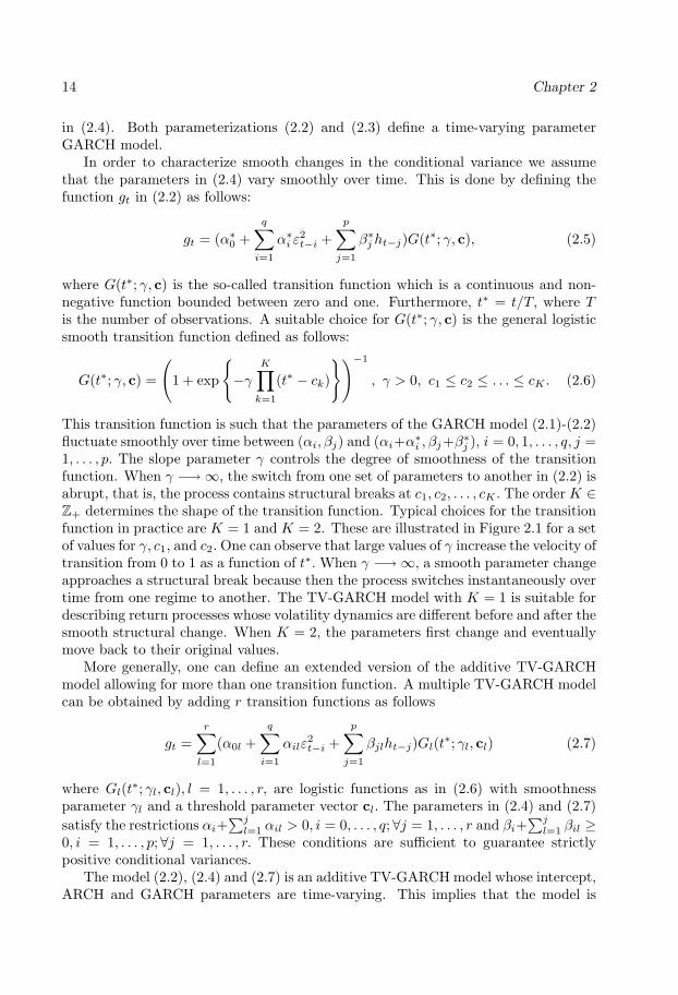
1, . . . , p. The slope parameter γ controls the degree of smoothness of the transitionfunction. When γ −→∞, the switch from one set of parameters to another in (2.2) isabrupt, that is, the process contains structural breaks at c1, c2, . . . , cK . The order K ∈Z+ determines the shape of the transition function. Typical choices for the transitionfunction in practice are K = 1 and K = 2. These are illustrated in Figure 2.1 for a setof values for γ, c1, and c2.One can observe that large values of γ increase the velocity oftransition from 0 to 1 as a function of t∗. When γ −→∞, a smooth parameter changeapproaches a structural break because then the process switches instantaneously overtime from one regime to another. The TV-GARCH model with K = 1 is suitable fordescribing return processes whose volatility dynamics are different before and after thesmooth structural change. When K = 2, the parameters first change and eventuallymove back to their original values.
More generally, one can define an extended version of the additive TV-GARCHmodel allowing for more than one transition function. A multiple TV-GARCH modelcan be obtained by adding r transition functions as follows
gt =r∑l=1
(α0l +q∑i=1
αilε2t−i +
p∑j=1
βjlht−j)Gl(t∗; γl, cl) (2.7)
where Gl(t∗; γl, cl), l = 1, . . . , r, are logistic functions as in (2.6) with smoothnessparameter γl and a threshold parameter vector cl. The parameters in (2.4) and (2.7)satisfy the restrictions αi+
∑jl=1 αil > 0, i = 0, . . . , q;∀j = 1, . . . , r and βi+
∑jl=1 βil ≥
0, i = 1, . . . , p;∀j = 1, . . . , r. These conditions are sufficient to guarantee strictlypositive conditional variances.
The model (2.2), (2.4) and (2.7) is an additive TV-GARCH model whose intercept,ARCH and GARCH parameters are time-varying. This implies that the model is

Modelling Conditional and Unconditional Heteroskedasticity 15
0.0 0.1 0.2 0.3 0.4 0.5 0.6 0.7 0.8 0.9 1.0
0.1
0.2
0.3
0.4
0.5
0.6
0.7
0.8
0.9
1.0
(a)
0.0 0.1 0.2 0.3 0.4 0.5 0.6 0.7 0.8 0.9 1.0
0.1
0.2
0.3
0.4
0.5
0.6
0.7
0.8
0.9
1.0
(b)
Figure 2.1 Plots of the logistic transition function (2.6) for: (a) K = 1 with locationparameter c1 = 0.5; and (b) K = 2 with location parameters c1 = 0.2 and c2 = 0.7for γ = 5, 10, 50, and 100 where the lowest value of γ corresponds to the smoothestfunction.
capable of accommodating systematic changes both in the “baseline volatility” (orunconditional variance) and in the amplitude of volatility clusters. Such changescannot be explained by a constant parameter GARCH model.
Function (2.7) with r > 1 is extremely flexible and probably makes the modeldifficult to estimate in practice. A more applicable but still flexible model is obtainedby only letting the “baseline volatility” or the intercept to change smoothly over time.This leads to the following definition for gt:
gt =r∑l=1
α0lGl(t∗; γl, cl). (2.8)
It may be mentioned that Baillie and Morana (2007) recently proposed a GARCHmodel which also has a deterministically time-varying intercept. It is modelled usingthe flexible functional form of Gallant (1984) based on the Fourier decomposition.Their model differs from our time-varying intercept model in the sense that it is inother respects a FIGARCH model, and the authors called it the Adaptive FIGARCHmodel.
In the GARCH(p, q) model, the unconditional variance of the returns is constantover time, that is, E(ε2t ) = α0/(1 −
∑qi=1 αi −
∑pj=1 βj) if and only if
∑qi=1 αi +∑p
j=1 βj < 1. However, this assumption is not consistent with the behaviour of thevolatilities of the stock market returns if the dynamic behaviour of volatility changesin the long run. The additive TV-GARCH model with a time-varying intercept iscapable of generating changes in the dynamics of the unconditional variance overtime. The model ( 2.2), (2.4) and (2.8) can be seen as a GARCH(p, q) model witha stochastic time-varying intercept fluctuating smoothly over time between α0 andα0 +
∑rl=1 α0lGl(t∗; γl, cl). Therefore, it can generate smooth changes over time in
the “baseline volatility”. Hence, such parameterization can explain the systematic

16 Chapter 2
movements of the conditional variance as in the GARCH model but relaxing theassumption of constancy of the unconditional volatility.
Consider again the model (2.2), (2.4) and (2.7) and assume that α0l = α0δl, αil =αiδl, i = 1, . . . , q;βjl = βjδl, j = 1, . . . , p. Furthermore, assume δl > 0, l = 1, . . . , r, ifthe transition function Gl(t∗; γl, cl) is increasing over time. For the case Gl(t∗; γl, cl) isa decreasing function assume
∑rl=1 δl < 1 for l = 1, . . . , r. Imposing these restrictions
on (2.7) and rewriting (2.2) yields
σ2t = ht(1 +
r∑l=1
δlGl(t∗; γl, cl)). (2.9)
Setting gt = 1 +∑rl=1 δlGl(t
∗; γl, cl) in (2.9) gives the multiplicative representation(2.3). It is thus seen to be a special case of the additive TV-GARCH model (2.2), (2.4)and (2.7). The multiplicative model has a straightforward interpretation. Writing itin terms of (2.1) as
φt = εt/g1/2t = ζtht
1/2 (2.10)
it is seen that φt has a constant unconditional variance Eht and, moreover, that φthas a standard stationary GARCH(p, q) representation ht. Turning (2.10) around,one obtains that ψt = εt/h
1/2t , t = 1, . . . , T, form a sequence of independent but
not identically distributed observations, as the unconditional variance of ψt changessmoothly as a function of time.
We consider properties of both time-varying GARCH specifications by generat-ing 1000 replications with Gaussian errors each with 5000 observations. Figure 2.2illustrates the relation of the average excess kurtosis of the two models given thepersistence and the time-varying constants α01 and δ1. The degree of persistence,measured by the sum α1 +β1, varies between 0.90 and 0.99. The range of parametersα01 and δ1 varies between 0 and 0.1 while α0 = 0.01. Interestingly, simply by assum-ing normality the proposed models are capable of generating higher kurtosis than thestandard GARCH model. Larger values of the time-varying constants generate largervalues of the excess kurtosis for both time-varying parameterizations. A high degreeof persistence is also able to reproduce heavy-tailed marginal distributions that areoften observed in financial return series.
The level of persistence generated by the TV-GARCH models is another prop-erty of interest. Figure 2.3 depicts the first 100 autocorrelations of absolute returnsof two simulated TV-GARCH processes. The autocorrelations for the additive andmultiplicative form are plotted in Figure 2.3(a) and Figure 2.3(b), respectively. Thesample length in both cases is 5000 observations. The artificial series are generatedwith α0 = 0.01, α1 = 0.05, α01 = 0.03, δ1 = 0.04, γ1 = 10 and c1 = 0.50. The dottedhorizontal lines represent the 95% confidence bounds corresponding to the ACF of aniid Gaussian process. A visual inspection of Figure 2.3 shows that both time-varyingspecifications can generate long-range dependence looking behaviour.
The dependence structure of each model is also illustrated by the empirical dis-tribution of the GPH estimates of the long-memory parameter d; see Geweke andPorter-Hudak (1983). The results obtained by using absolute values of the returns

Modelling Conditional and Unconditional Heteroskedasticity 17E
xces
s ku
rtos
is
Persistence α 010.01 0.03 0.05 0.07 0.09
0.91
0.93
0.95
0.97
0.99
0.5
1.0
1.5
2.0
(a)
δ1
Exc
ess
kurt
osis
Persistence0.01 0.03 0.05 0.07 0.09
0.91
0.93
0.95
0.97
0.99
100
200
300
400
500
(b)
Figure 2.2 Plots of the excess kurtosis, persistence and the constants α01 and δ1for: (a) an additive TV-GARCH model with a time-varying constant; and (b) amultiplicative TV-GARCH model.
0 10 20 30 40 50 60 70 80 90 100
0.0
0.1
0.2
0.3
0.4
0.5
(a)
0 10 20 30 40 50 60 70 80 90 100
0.0
0.1
0.2
0.3
0.4
0.5
(b)
Figure 2.3 Sample autocorrelation functions of absolute returns with the 95% con-fidence bounds for: (a) an additive TV-GARCH model with a time-varying constant;and (b) a multiplicative TV-GARCH model.

18 Chapter 2
−0.1 0.0 0.1 0.2 0.3 0.4 0.5
1
2
3
4
5
6
(a)
0.2 0.3 0.4 0.5 0.6 0.7
1
2
3
4
5
6
(b)
0.2 0.3 0.4 0.5 0.6 0.7 0.8 0.9
1
2
3
4
5
6
(c)
Figure 2.4 Histograms of the GPH long memory parameter estimates for: (a) aGARCH model; (b) an additive TV-GARCH model with a time-varying constant;and (c) a multiplicative TV-GARCH model. The artificial series are generated withα0 = 0.01, α1 = 0.05, β1 = 0.90, α01 = 0.03, δ1 = 0.04, γ1 = 10 and c1 = 0.50 for asample of 5000 observations based on 1000 replications.
are displayed in Figure 2.4. The standard GARCH model is known to have a shortmemory in the sense that the theoretical autocorrelation function decays to zero atan exponential rate. The exponential decay turns out to be too fast if one wantsto adequately describe the high persistence observed in financial data. This may beseen from Figure 2.4(a). If the data are generated by the standard GARCH model,the estimates of the long memory parameter are rather close to zero. However, whenthe intercept of the GARCH model changes smoothly over time, the degree of thelong-memory dependence in the data increases. This is seen from the fact that theempirical distribution for the GPH estimates in Figure 2.4(b) has shifted to the right.As Figure 2.4(c) shows, this effect is even more evident for the TV-GARCH with amultiplicative time-varying structure as more than one half of the probability massof the empirical distribution of the long-memory parameter is located in the nonsta-tionary area, d > 0.5.

Modelling Conditional and Unconditional Heteroskedasticity 19
2.3 Testing parameter constancy
2.3.1 Testing against an additive alternative
Against the background discussed above, testing parameter constancy is an importanttool for checking the adequacy of a GARCH model. If one rejects parameter constancyagainst a GARCH model with time-varying parameters one may conclude that thestructure of the dynamics of volatility is changing over time. Other interpretationscannot be excluded, however, because a rejection of a null hypothesis does not implythat the alternative hypothesis is true. In this section, we propose two parameterconstancy tests that allow the parameters to change smoothly over time under thealternative. The first one tests parameter constancy of the GARCH model againstan additive TV-GARCH specification. This idea has previously been considered byLundbergh and Terasvirta (2002). The second one is a test of constant unconditionalvariance against the alternative that the variance changes smoothly over time.
We shall first look at the additive alternative where the nonstationary componentgt is defined in (2.5). In order to derive the test statistic rewrite the model as
εt = ζtht1/2, εt|Ft−1 ∼ N(0, ht)
ht = α0 +q∑i=1
αiε2t−i +
p∑j=1
βjht−j
+ (α01 +q∑i=1
αi1ε2t−i +
p∑j=1
βj1ht−j)G(t∗; γ, c) (2.11)
where, for simplicity, r = 1 and Ft−1 is the information set containing all informa-tion until t − 1. The null hypothesis of parameter constancy corresponds to testingH0 : γ = 0 against H1 : γ > 0 in (2.11). Under the null hypothesis, gt ≡ 1/2. Onecan see that model (2.11) is only identified under the alternative. In particular, whenγ = 0, the parameters αi1, i = 0, . . . , q, and βj1, j = 1, . . . , p, as well as c are notidentified. This makes the standard asymptotic inference invalid as the test statisticshave a nonstandard asymptotic null distribution. This identification problem wasfirst considered in Davies (1977) and more recently, among others, in Hansen (1996).
In this paper, we circumvent the identification problem following Luukkonen,Saikkonen, and Terasvirta (1988). Thus we replace the transition function by itsfirst-order Taylor approximation around γ = 0. Without losing generality, we replaceG(t∗; γ, c) by G(t∗; γ, c) = G(t∗; γ, c)−1/2 for notational convenience. From Taylor’s

20 Chapter 2
theorem one obtains
G(t∗; γ, c) = G(t∗; 0, c) +∂G(t∗; 0, c)
∂γγ +R(t∗; γ, c)
=14γ
K∏k=1
(t∗ − ck) +R(t∗; γ, c)
=K∑k=0
γck(t∗)k +R(t∗; γ, c) (2.12)
where R(t∗; γ, c) is the remainder term. Replacing G(t∗; γ, c) in (2.11) by (2.12) andrearranging terms gives
ht = α∗0 +q∑i=1
α∗i ε2t−i +
p∑j=1
β∗j ht−j
+K∑k=1
(ωk(t∗)k +q∑i=1
ϕik(t∗)kε2t−i +p∑j=1
λjk(t∗)kht−j) +R∗1 (2.13)
where α∗s = αs+γαs1c0, s = 0, . . . , q, β∗j = βj+γβj1c0, j = 1, . . . , p, ωk = γα01ck, ϕik =γαi1ck, i = 1, . . . , q, and λjk = γβj1ck, k = 1, . . . ,K. The parameters ck, k = 0, . . . ,K,are functions of the original location parameters ck. In particular, c0 = 1
4
∏Kk=1 ck and
cK = 14 . Under H0, the remainder R∗1 ≡ 0, so it does not affect the asymptotic null
distribution of the test statistic. Using the reparameterization (2.13) it follows thatthe null hypothesis of parameter constancy becomes
H′0 : ωk = ϕik = λjk = 0, k = 1, . . . ,K, i = 1, . . . , q, j = 1, . . . , p. (2.14)
This hypothesis can be tested by a standard LM test. One can also test constancy ofa subset of parameters. For example, it may be assumed that αi1 = 0, i = 1, . . . , q,and βj1 = 0, j = 1, . . . , p, which means that only the intercept is time-varying underthe alternative. In this case the null hypothesis reduces to H′0 : ωk = 0, k = 1, . . . ,K.
In Theorem 1 we present the LM-type statistic for testing parameter constancyagainst the additive TV-GARCH specification. Under the null hypothesis, the “hats”indicate maximum likelihood estimators and h0
t denotes the conditional variance attime t estimated under H0.
Theorem 1 Consider the model (2.13) and let θ1 = (α∗0, α∗1, . . . , α
∗q , β∗1 , . . . , β
∗p)′
and θ2 = (ω′,ϕ′i,λ′j)′ where ω = (ω1, . . . , ωK)′,ϕi = (ϕi1, . . . , ϕiK)′ and λj =
(λj1, . . . , λjK)′ for i = 1, . . . , q and j = 1, . . . , p. In addition, denote zt = (1, ε2t−1, . . . ,ε2t−q, ht−1, . . . , ht−p)′,Z1t = [t∗kε2t−i](k = 1, . . . ,K, i = 1, . . . , q) and Z2t = [t∗kht−j ](k = 1, . . . ,K, j = 1, . . . , p). Furthermore, assume that the maximum likelihood esti-mator of θ1 is asymptotically normal. Under H0 : θ2 = 0, the LM type statistic
ξLM =12
T∑t=1
utx′2t
T∑t=1
x2tx′2t −T∑t=1
x2tx′1t
(T∑t=1
x1tx′1t
)−1 T∑t=1
x1tx′2t
−1
T∑t=1
utx2t
(2.15)

Modelling Conditional and Unconditional Heteroskedasticity 21
is asymptotically χ2-distributed with dim(θ2) degrees of freedom, where ut = ε2t/h0t−1,
x1t =1
h0t
∂ht∂θ1
∣∣∣∣∣H0
= (h0t )−1(zt +
p∑j=1
β∗j∂ht−j∂θ1
∣∣∣∣∣H0
) (2.16)
and
x2t =1
h0t
∂ht∂θ2
∣∣∣∣∣H0
= (h0t )−1((t∗, . . . , t∗K , (vec Z1t)′, (vec Z2t)′)′ +
p∑j=1
β∗j∂ht−j∂θ2
∣∣∣∣∣H0
)
(2.17)Proof. See Appendix A.
In practice, the test of Theorem 1 may be carried out in a straightforward wayusing an auxiliary least squares regression. Thus:
1. Estimate consistently the parameters of the conditional variance under the nullhypothesis, and compute ut = ε2t/h
0t − 1, t = 1, . . . , T, and the residual sum of
squares, SSR0 =∑Tt=1 u
2t .
2. Regress ut on x′1t and x′2t, t = 1, . . . , T, and compute the sum of the squaredresiduals, SSR1.
3. Compute the χ2 test statistic as
ξLM =T (SSR0 − SSR1)
SSR0.
As a computational detail, note that ∂ht/∂θ1|H0 and ∂ht/∂θ2|H0 in (2.16) and(2.17) are obtained recursively in connection with the parameter estimation, whereit is assumed that ∂ht/∂θ1|H0 = 0 and ∂ht/∂θ2|H0 = 0 for t = 0,−1, . . .. We shallcall our LM test statistic LMK , where K indicates the order of the polynomial in theexponent of the transition function and the tests carried out by means of an auxiliaryregression are called LM-type tests.
It should also be mentioned that a robust version of the test statistics (2.15)can be derived when ζt are not identically distributed. One can construct a robustversion using the procedure by Wooldridge (1990,1991). This test can be carried outas follows:
1. Estimate by quasi maximum likelihood the conditional variance under H0, com-pute ε2t/h
0t − 1, x′1t and x′2t, t = 1, . . . , T.
2. Regress x2t on x1t, and compute the (dimθ2×1) residual vectors rt, t = 1, . . . , T.
3. Regress 1 on(ε2t/h
0t − 1
)rt and compute the residual sum of squares SSR0 from
this regression. Under the null hypothesis, the test statistic ξLMR= T − SSR0
has an asymptotic χ2 distribution with dimθ2 degrees of freedom.

22 Chapter 2
One may extend Theorem 1 to the case where the model has been estimated withr − 1 transition functions and one wants to test r − 1 against r transitions. For thatpurpose, consider the model
εt = ζtht1/2, εt|Ft−1 ∼ N(0, ht)
ht = (θ0 +r−1∑l=1
θ1lGl(t∗; γl, cl))′zt + θ′1rGr(t∗; γr, cr)zt (2.18)
where θ0 = (α0, α1, . . . , αq, β1, . . . , βp)′,θ1l = (α0l, α1l, . . . , αql, β1l, . . . , βpl)′, l = 1, . . . ,r − 1, r, and zt = (1, ε2t−1, . . . , ε
2t−q, ht−1, . . . , ht−p)′. The null hypothesis is then
H0 : γr = 0. Again, model (2.18) is not identified under the null hypothesis. To cir-cumvent the problem we proceed as before and expand the logistic functionGr(t∗; γr, cr)into a first-order Taylor approximation around γr = 0. After rearranging terms wehave
ht = (η +r−1∑l=1
θ1lGl(t∗; γl, cl))′zt +K∑k=1
µ′k(t∗)kzt +R∗2 (2.19)
where η = θ0 + γrθ1r c0,µk = γrθ1r ck, k = 1, . . . ,K. The test statistic is based onthe following corollary of Theorem 1.
Corollary 2 Consider the model (2.19) and let θ1 = (η′,θ′1l, γl, c′l)′ and θ2 = (µ′1, . . . ,
µ′K)′. In addition, denote zt = (1, ε2t−1, . . . , ε2t−q, ht−1, . . . , ht−p)′,Z1t = [t∗kε2t−i](k =
1, . . . ,K, i = 1, . . . , q),Z2t = [t∗kht−j ](k = 1, . . . ,K, j = 1, . . . , p) and Gl(t∗) ≡Gl(t∗; γl, cl). Assume that the maximum likelihood estimator of (θ′0,θ
′11, . . . ,θ
′1,r−1, γ1,
. . . , γr−1, c′1, . . . , c′r−1)′ is asymptotically normal. Under H0 : θ2 = 0, the LM type
statistic (2.15) with ut = ε2t/h0t − 1,
x1t =1
h0t
∂ht∂θ1
∣∣∣∣∣H0
= (h0t )−1(zt +
r−1∑l=1
ztGl(t∗) +r−1∑l=1
θ′1lzt
∂Gl(t∗)∂θ1
+p∑j=1
(βj +r−1∑l=1
β∗jlGl(t∗))
∂ht−j∂θ1
∣∣∣∣∣H0
)
and
x2t =1
h0t
∂ht∂θ2
∣∣∣∣∣H0
= (h0t )−1((t∗, . . . , t∗K , (vecZ1t)′, (vecZ2t)
′)′ +p∑j=1
(βj +r−1∑l=1
β∗jlGl(t∗))
∂ht−j∂θ2
∣∣∣∣∣H0
)
has an asymptotic χ2−distribution with dim(θ2) degrees of freedom.
Remark 3 The assumption of asymptotic normality in this corollary remains unver-ified. The existing asymptotic theory of nonlinear GARCH models does not cover the

Modelling Conditional and Unconditional Heteroskedasticity 23
case where the transition function is a function of time. Besides, Meitz and Saikko-nen (in press) who have worked out asymptotic theory for smooth transition GARCHmodels, have only obtained results on ergodicity and stationarity. Asymptotic normal-ity of maximum likelihood estimators has not even been proven for ’standard’ smoothtransition GARCH models in which the transition variable is a stochastic variable.For these reasons, showing asymptotic normality of θ1 in (2.19) is beyond the scopeof this paper. Two things should be emphasized in this context. First, sequentialtesting to find r is just a model selection device analogous to model selection crite-ria such as AIC or BIC. The p-values of the tests are simply indicators helping themodeller to choose the number of transitions. Second, our simulation results do notcontradict the assumption that the asymptotic null distribution of the test statistic isa χ2-distribution.
2.3.2 Testing against a multiplicative alternative
In order to consider the problem of testing parameter constancy in the unconditionalvariance assume that the error term is parameterized as
εt = ζtht1/2
where ht is a GARCH(p, q) model as in (2.4) and ζt is a time-varying random variablesatisfying
ζt = ztg1/2t
such that {zt} is a sequence of independent standard normal variables and gt =1 +
∑rl=1 δlGl(t
∗; γl, cl). This formulation allows the unconditional variance of ζt andthus εt to change smoothly over time. As already mentioned, {ζt} is a sequence ofindependent variables. The null hypothesis of constant unconditional variance is thenH0 : δl = 0, l = 1, . . . , r. For the purpose of deriving the test statistic consider r = 1and rewrite the model as follows:
εt = zt(htgt)1/2, εt|Ft−1 ∼ N(0, htgt)
htgt = (α0 +q∑i=1
αiε2t−i +
p∑j=1
βjht−j)(1 + δ1G(t∗; γ, c)). (2.20)
The null hypothesis of constant unconditional variance equals H0 : γ = 0 againstH1 : γ > 0. In testing this hypothesis we encounter the same identification problemas the one present in testing parameter constancy against an additive TV-GARCHprocess. Even here, our solution consists of approximating the transition functionwith a Taylor expansion around γ = 0. Proceeding as before, we reparameterizeequation (2.20) as follows:
htgt = (α0 +q∑i=1
αiε2t−i +
p∑j=1
βjht−j)(δ0 +K∑k=1
ωk(t∗)k +R∗3) (2.21)

24 Chapter 2
where δ0 = 1 + γδ1c0 and ωk = γδ1ck, k = 1, . . . ,K. Under the null hypothesis, theremainder R∗3 ≡ 0 and does not affect the distribution theory. The null hypothesis ofparameter constancy for the multiplicative structure becomes
H′0 : ωk = 0, k = 1, . . . ,K.
The following corollary of Theorem 1 defines the LM-type test statistic for testingparameter constancy in the unconditional variance. The notation g0
t denotes theestimated gt evaluated under H0.
Corollary 4 Consider the model (2.21) and let θ1 = (α0, α1, . . . , αq, β1, . . . , βp)′ andθ2 = (ω1, . . . , ωK)′. In addition, denote zt = (1, ε2t−1, . . . , ε
2t−q, ht−1, . . . , ht−p)′ and
gt = 1 + δ1G(t∗; γ, c). Under H0 : θ2 = 0, the LM type statistic (2.15) with ut =ε2t/h
0t − 1,
x1t =1
h0t
∂ht∂θ1
∣∣∣∣∣H0
= (h0t )−1(zt +
p∑j=1
β∗j∂ht−j∂θ1
∣∣∣∣∣H0
)
and
x2t =1g0t
∂gt∂θ2
∣∣∣∣H0
= (t∗, t∗2, . . . , t∗K)′
has an asymptotic χ2−distribution with dim(θ2) degrees of freedom.
Once the TV-GARCH model with a single transition has been estimated we maywant to investigate the possibility of remaining parameter nonconstancy in the un-conditional variance. This is important from the model specification point of view.Thus, similarly to the additive structure, the previous corollary may be extended tothe case where we want to test r = 1 against r ≥ 2. To derive the test, consider themodel
εt = zt(htgt)1/2, εt|Ft−1 ∼ N(0, htgt)
htgt = (α0 +q∑i=1
αiε2t−i +
p∑j=1
βjht−j)(1 +∑2
l=1δlGl(t∗; γl, cl)). (2.22)
The null hypothesis is H0 : γ2 = 0. Again, model (2.22) is only identified underthe alternative. The solution to the identification problem consists of replacing thetransition function G2(t∗; γ2, c2) by a Taylor approximation around γ2 = 0. After areparameterization, the resulting model is
htgt = (α0 +q∑i=1
αiε2t−i+
p∑j=1
βjht−j)(δ0 + δ1G1(t∗; γ1, c1) +K∑k=1
ωk(t∗)k +R∗4) (2.23)
where δ0 = 1 + γ2δ2c0 and ωk = γ2δ2ck, k = 1, . . . ,K. Under the null, the remainderR∗4 ≡ 0.
The next corollary to Theorem 1 gives the test statistic.

Modelling Conditional and Unconditional Heteroskedasticity 25
Corollary 5 Consider the model (2.23) and let θ1 = (α0, α1, . . . , αq, β1, . . . , βp, δ1, γ1,c′1)′ and θ2 = (ω1, . . . , ωK)′. In addition, denote zt = (1, ε2t−1, . . . , ε
2t−q, ht−1, . . . , ht−p)′
and gt = 1 +∑2l=1 δlGl(t
∗; γl, cl). Under H0 : θ2 = 0, the LM type statistic (2.15)with ut = ε2t/h
0t g
0t − 1,
x1t =1
h0t
∂ht∂θ1
∣∣∣∣∣H0
= (h0t )−1(ztg0
t + h0t
∂g0t
∂θ1+
p∑j=1
βj g0t
∂ht−j∂θ1
∣∣∣∣∣H0
)
and
x2t =1g0t
∂gt∂θ2
∣∣∣∣H0
= (g0t )−1(t∗, t∗2, . . . , t∗K)′
has an asymptotic χ2−distribution with dim(θ2) degrees of freedom.
Remark 6 The previous remark is valid even here.
A special case of this test, in which ht ≡ α0, will be used in the specification ofmultiplicative TV-GARCH models in Subsection 2.4.2.
2.4 Model specification
We propose a model-building cycle for TV-GARCH models identical to the specific-to-general strategy for nonlinear models recommended by Granger (1993) or Terasvirta(1998), among others. The idea is to begin with a parsimonious model and proceedto more complicated ones until the evaluation techniques indicate that an adequatemodel has been obtained. Adapting this approach to the present situation means de-termining the number of smooth transitions sequentially by LM-type tests discussedin Section 2.3. These tests can be used to build a GARCH model with time-varyingparameters using either the additional or the multiplicative structure. We start offwith a restricted specification and gradually increase the number of transition func-tions as long as the hypothesis of parameter constancy is rejected. The final model isestimated after the first non-rejection of the null hypothesis and evaluated through asequence of misspecification tests.
2.4.1 Specification of additive TV-GARCH models
In order to describe the specification procedure for TV-GARCH models with an addi-tional time-varying structure, we consider the function gt defined in (2.7) such that allparameters are changing smoothly over time. However, the strategy may also be ap-plied to a more restrictive functions such as gt in (2.8). The time-varying conditionalvariance equals
ht = α0 +q∑i=1
αiε2t−i +
p∑j=1
βjht−j +r∑l=1
(α0l +q∑i=1
αilε2t−i +
p∑j=1
βjlht−j)Gl(t∗; γl, cl),
(2.24)

26 Chapter 2
where the transition function Gl(t∗; γl, cl) is defined in (2.6).Our specification procedure for building additive TV-GARCH models contains the
following stages:
1. Check for the presence of conditional heteroskedasticity by testing the null hy-pothesis of no ARCH against high-order ARCH. When the order of the ARCHprocess is sufficiently high, the standard LM test has adequate power againstGARCH. If the null hypothesis is rejected, model the conditional variance by aGARCH(1,1) model. Evaluate the estimated GARCH(1,1) model by misspeci-fication tests and, if necessary, expand it to a higher-order model. The squaredstandardized errors of the selected GARCH model should be free of serial cor-relation. Neglected autocorrelation may bias tests of parameter constancy.
2. Test the final GARCH model against the alternative of smoothly changing pa-rameters over time using the LM-type statistic described in Theorem 1. Ifparameter constancy is rejected at a predetermined significance level α, esti-mate the TV-GARCH model (2.24) with a single transition function. If the nullhypothesis of parameter constancy in (2.14) is rejected, the problem of choosingthe order of the polynomial of the transition function arises. For the specifica-tion of K, we propose a model selection rule based on a sequence of nested testsas in Terasvirta (1994) and Lin and Terasvirta (1994). Assume K = 3 to ensurea parameterization sufficiently flexible for G(t∗; γ, c). If parameter constancy isrejected, test the following sequence of hypotheses:
H03 : ω3 = 0, ϕi3 = 0, λj3 = 0,H02 : ω2 = 0, ϕi2 = 0, λj2 = 0 | ω3 = 0, ϕi3 = 0, λj3 = 0,H01 : ω1 = 0, ϕi1 = 0, λj1 = 0 | ω2 = ω3 = 0, ϕi2 = ϕi3 = 0, λj2 = λj3 = 0,
where i = 1, . . . , q, j = 1, . . . , p, in (2.13), by means of LM-type tests. Theresults of this test sequence may be used as follows. If H01 and H03 are rejectedmore strongly, measured by p-values, than H02, then either K = 1 or K = 3.If testing H02 yields the strongest rejection, the choice is K = 2. Furthermore,if only H01 is rejected at the appropriate significance level or is rejected clearlymore strongly than the other two null hypotheses, then the modeller shouldchoose K = 1. Visual inspection of the return series is also helpful in makinga decision about K. The rules or suggestions based on p-values are based onexpressions of the parameters ωk, ϕik and λjk in the auxiliary regression asfunctions of the original parameters at different values of K. The test sequenceis analogous to that proposed in Terasvirta (1994) for specifying the type of thesmooth transition autoregressive model, where the choice is between K = 1 andK = 2.
3. Test the TV-GARCH model with one transition function against the TV-GARCHmodel with two transition functions at the significance level ατ, 0 < τ < 1. Thesignificance level is decreased giving a preference for parsimonious models. Theoverall significance level of the sequence of tests may be approximated by the

Modelling Conditional and Unconditional Heteroskedasticity 27
Bonferroni upper bound. The user can choose the value for τ. In our simu-lations we set τ = 1/2. If the null hypothesis is rejected, specify K for thenext transition and estimate the TV-GARCH model (2.12) with two transitionfunctions.
4. Proceed sequentially by testing the TV-GARCH model with r − 1 transitionfunctions against the TV-GARCH model with r transitions at the significancelevel ατ r−1 until the first non-rejection of the null hypothesis. Evaluate theselected model by misspecification tests and once it passes them accept it as thefinal model. In the opposite case, modify the specification of the model or tryanother family of models.
2.4.2 Specification of multiplicative TV-GARCH models
The specific-to-general approach for specifying TV-GARCH models with a multiplica-tive time-varying component consists in first modelling the unconditional variance asfollows:
1. Use the LM-type statistic developed in Section 2.3.2 to test the null hypothesisof constant variance against a time-varying unconditional variance with a singletransition function at the significance level α. First, assume ht = α0 and testH10 : gt ≡ 1 against H11 : gt = 1 + δ1G1(t∗; γ1, c1). In case of a rejection, testH20 : gt = 1 + δ1G1(t∗; γ1, c1) against H21 : gt = 1 +
∑2l=1 δlGl(t
∗; γl, cl) atthe significance level ατ, 0 < τ < 1. Continue until the first non-rejection ofthe null hypothesis. The significance level is reduced at each step of the testingprocedure and converging to zero for reasons previously mentioned.
2. After specifying gt, test the null hypothesis of no conditional heteroskedasticityin {ζt}. If it is rejected, model the conditional variance ht of the standardizedvariable εt/g
1/2t in the standard fashion, such that
ht = α∗0 +q∑i=1
αi
(ε2t−igt−i
)+
p∑j=1
βjht−j . (2.25)
3. The estimated model is evaluated by means of LM-type diagnostic tests pro-posed in Subsection 2.6.1. If the model passes all the misspecification tests,tentatively accept it. Otherwise, modify it or consider another family of volatil-ity models.
2.5 Estimation of the TV-GARCH model
Suppose that εt is generated by a GARCH model with a time-varying structure de-scribed in Section 2.2. Let ht = ht(θ1) and gt = gt(θ2) where θ1 = (α0, α1, . . . , αq, β1,. . . , βp)′ and θ2 = (δ′,α′1, . . . ,α
′r,β′1, . . . ,β
′r, γ1, . . . , γr, c′1, . . . , c
′r)′ with δ = (δ1, . . . ,

28 Chapter 2
δr)′,αi = (α1i, . . . , αqi)′ and βi = (β1i, . . . , βpi)′, i = 1, . . . , r. For the additive pa-rameterization, δ = 0 and for the multiplicative one, αi = 0 and βi = 0. Thequasi maximum likelihood (QML) estimator θ = (θ
′1,θ′2)′ is obtained maximizing∑T
t=1 `t(θ) with respect to θ where the log-likelihood for observation t equals
`t(θ) = −12
ln 2π − 12
ln{ht(θ1) + gt(θ2)} − 12
ε2tht(θ1) + gt(θ2)
(2.26)
for the additive TV-GARCH model or
`t(θ) = −12
ln 2π − 12{lnht(θ1) + ln gt(θ2)} − 1
2ε2t
ht(θ1)gt(θ2)(2.27)
for the multiplicative TV-GARCH model.The asymptotic properties of the QML estimators for the GARCH(p, q) process
have been studied, among others, by Ling and Li (1997). They showed that theQML estimators are consistent and asymptotic normal provided that Eε4t <∞. Lingand McAleer (2003) established consistency for the global maximum of QML estima-tors under the condition Eε2t < ∞. Berkes, Horvath, and Kokoszka (2003) obtainedconsistency of the QML estimators assuming Eε2t < ∞ and asymptotic normalityby assuming Eε4t < ∞. These results have in common the assumption that the pro-cess yt is stationary and ergodic such that the laws of large numbers apply. Morerecently, Jensen and Rahbek (2004) relaxed this assumption and allowed the param-eters to lie in the region where the process is nonstationary. They showed that forthe GARCH(1,1) case, under a finite conditional variance for ζ2
t , consistency andasymptotic normality still hold independently of whether the process yt is stationaryor not. As already mentioned, asymptotic normality for the parameter estimators ofthe TV-GARCH models has not yet been proven.
Three remarks are in order regarding numerical aspects of the estimation of TV-GARCH models. The first one concerns the accuracy of the slope estimates when thetrue parameters γl are very large. In order to achieve an accurate estimate for a largeγl, the number of observations of the transition variable in the neighbourhood of clmust be very large. This is due to the fact that even large changes in γl only havean effect on the transition function in a small neighbourhood of cl. But then, for thesame reason for large γl it is sufficient to obtain an estimate that is large; whetheror not it is very accurate is not of utmost importance. Note that if γl is large, an“insignificant” γl is an indication of a large γl, not of γl ≡ 0. Besides, because of theidentification problem the t-ratio does not have its standard asymptotic distributionwhen γl ≡ 0. A more serious problem is that large estimates for the smoothnessparameter γl may lead to numerical problems when carrying out parameter constancytests. A simple solution, suggested in Eitrheim and Terasvirta (1996), is to omit thoseelements of the score that are partial derivatives with respect to the parameters inthe transition function. This can be done without significantly affecting the value ofthe test statistic.
The second comment has to do with the computation of the derivatives of thelog-likelihood function. Many of the existing optimization algorithms require the
Modelling Conditional and Unconditional Heteroskedasticity 29
computation of at least the first and, in some cases, also the second derivatives ofthe log-likelihood function. It is common practice to use numerical derivates that arerelatively fast to compute and reliable, and the derivation of exact analytic deriva-tives is avoided. Fiorentini, Calzolari, and Panattoni (1996), however, encourage theemployment of analytic derivatives, because that leads to fewer iterations than opti-mization with numerical derivatives. Furthermore, the use of analytic derivatives alsoimproves the accuracy of the estimates of the standard errors of the parameter esti-mates. Consequently, we use analytic first derivatives in all the computations, bothin calculating values of the test statistics and in estimating TV-GARCH models.
The third remark is related to the manner in which the parameter estimates areobtained. The parameters in the additive TV-GARCH model are estimated simulta-neously by full conditional maximum likelihood. In this context, care is required inthe estimation. Since the log-likelihood (2.27) may contain several local maxima, itis advisable to initiate the estimation from different sets of starting-values before set-tling for the final parameter estimates. Numerical problems in the estimation of themultiplicative TV-GARCH model can be alleviated by concentrating the likelihooditeratively. This considerably reduces the dimensionality problem and is computation-ally much easier than maximizing the log-likelihood with respect to all parameterssimultaneously. The estimation of the TV-GARCH model with multiplicative struc-ture can be simplified since the log-likelihood can be decomposed into two separatesets of parameters: the GARCH and the time-varying parameter vectors. The esti-mation is divided into two steps which are then repeated one after the other. Theiterations start by first estimating θ2, assuming ht to be a positive constant, for in-stance ht = σ2 = T−1
∑Tt=1 ε
2t , and continue by estimating θ1, given the estimates
of θ2. The estimate of θ1 will then be used for re-estimating θ2, and so on. Theiterative two-stage estimation procedure is terminated when a local maximum of thelog-likelihood has been reached.
2.6 Misspecification testing of TV-GARCH models
The final step of the modelling strategy consists of evaluating the adequacy of theestimated TV-GARCH model by means of a sequence of misspecification tests. Weshall assume that the true process of either the additive or the multiplicative time-varying variance is misspecified. The general idea is to construct an augmented versionof the TV-GARCH model by introducing a new component ft = f(vt;θ3) into theoriginal model. This component is a function that is at least twice continuouslydifferentiable with respect to the elements of θ3, vector of additional parameters.The vector vt is a vector of omitted random variables, and its definition varies fromone test to the next.
2.6.1 Misspecification tests for the multiplicative model
The misspecification tests considered here may be divided into three categories. Thefirst two correspond to additive and the third one to multiplicative misspecification.
30 Chapter 2
Let ht = ht(θ1) and gt = gt(θ2), such that the parameter vectors θi, i = 1, 2,represent the parameters belonging to ht = α0 +
∑qi=1 αiε
2t−i +
∑pj=1 βjht−j and
gt = 1 +∑rl=1 δlGl(t
∗; γl, cl). Under H0 : θ3 = 0, the augmented model reduces tothe multiplicative TV-GARCH model.
Additive misspecification - case 1
The first category of tests assumes that, under the alternative hypothesis, the originalTV-GARCH model may be extended by assuming
εt = ζt(ht + ft)1/2g1/2t . (2.28)
Under the null hypothesis, ft ≡ 0, which is equivalent to θ3 = 0. If gt ≡ 1, the testcollapses into the additive misspecification test in Lundbergh and Terasvirta (2002).At least three types of alternative hypotheses can be considered within this family oftests. The test of the GARCH(p, q) component against higher-order alternatives aswell as the test against a smooth transition GARCH (ST-GARCH) and, furthermore,the test against an asymmetric component (GJR-GARCH) belong to the additiveclass (2.28).
The log-likelihood function for observation t of model (2.28) is
`t = −12
ln 2π − 12{ln(ht + ft) + ln gt} −
ε2t2(ht + ft)gt
. (2.29)
When the estimated multiplicative TV-GARCH model is tested against the differenttypes of alternatives, the first component of the score corresponding to θ1 and θ2,evaluated under H0, is equal to
∂`t∂θ
∣∣∣∣H0
=12
(ε2thtgt
− 1)
x1t
where x1t =(
1ht
∂ht
∂θ′1, 1gt
∂gt
∂θ′2
)′and the parameter vector θ is partitioned as θ =
(θ′1,θ′2)′. The estimated quantities for ∂ht
∂θ1|H0 and ∂gt
∂θ2|H0 are defined as
∂ht∂θ1
∣∣∣∣∣H0
= zt +p∑j=1
βj∂ht−j∂θ1
∣∣∣∣∣H0
(2.30)
∂gt∂θ2
∣∣∣∣H0
=r∑l=1
Gl(t∗; γl, cl) +r∑l=1
δl∂Gl(t∗; γl, cl)
∂θ2. (2.31)
The differences show up in the partial derivatives of (2.29) with respect to θ3. Itfollows that the additional block of the score for observation t due to θ3 has the form
∂`t∂θ3
=12
(ε2t
(ht + ft)gt− 1)
1ht
∂ft∂θ3
Modelling Conditional and Unconditional Heteroskedasticity 31
so that, under H0,∂`t∂θ3
∣∣∣∣H0
=12
(ε2thtgt
− 1)
1ht
∂ft∂θ3
∣∣∣∣H0
where ∂ft
∂θ3= vt. The resulting LM test may be easily performed using an auxiliary
regression as in Section 2.3. In terms of previous notation, we have
x1t =
(1
h0t
∂ht
∂θ′1
∣∣∣∣∣H0
,1g0t
∂gt
∂θ′2
∣∣∣∣H0
)′(2.32)
x2t =1
h0t
∂ft∂θ3
∣∣∣∣∣H0
=vth0t
(2.33)
where ∂ht
∂θ1|H0 and ∂gt
∂θ2|H0 are as in (2.30) and (2.31), respectively. We shall now
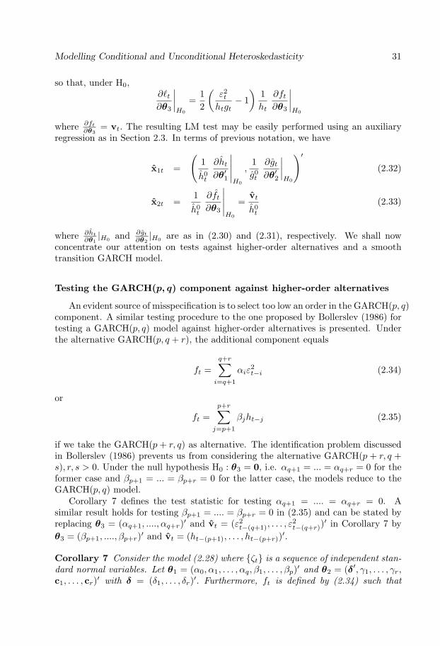
concentrate our attention on tests against higher-order alternatives and a smoothtransition GARCH model.
Testing the GARCH(p, q) component against higher-order alternatives
An evident source of misspecification is to select too low an order in the GARCH(p, q)component. A similar testing procedure to the one proposed by Bollerslev (1986) fortesting a GARCH(p, q) model against higher-order alternatives is presented. Underthe alternative GARCH(p, q + r), the additional component equals
ft =q+r∑i=q+1
αiε2t−i (2.34)
or
ft =p+r∑j=p+1
βjht−j (2.35)
if we take the GARCH(p+ r, q) as alternative. The identification problem discussedin Bollerslev (1986) prevents us from considering the alternative GARCH(p + r, q +s), r, s > 0. Under the null hypothesis H0 : θ3 = 0, i.e. αq+1 = ... = αq+r = 0 for theformer case and βp+1 = ... = βp+r = 0 for the latter case, the models reduce to theGARCH(p, q) model.
Corollary 7 defines the test statistic for testing αq+1 = .... = αq+r = 0. Asimilar result holds for testing βp+1 = .... = βp+r = 0 in (2.35) and can be stated byreplacing θ3 = (αq+1, ...., αq+r)′ and vt = (ε2t−(q+1), . . . , ε
2t−(q+r))
′ in Corollary 7 byθ3 = (βp+1, ...., βp+r)′ and vt = (ht−(p+1), . . . , ht−(p+r))′.
Corollary 7 Consider the model (2.28) where {ζt} is a sequence of independent stan-dard normal variables. Let θ1 = (α0, α1, . . . , αq, β1, . . . , βp)′ and θ2 = (δ′, γ1, . . . , γr,c1, . . . , cr)′ with δ = (δ1, . . . , δr)′. Furthermore, ft is defined by (2.34) such that

32 Chapter 2
θ3 = (αq+1, . . . , αq+r)′ and vt = (ε2t−(q+1), . . . , ε2t−(q+r))
′. Assume that the maxi-mum likelihood estimators of the parameters of (2.28) are asymptotically normal whenH0 : θ3 = 0 is valid. Thus, under this null hypothesis, the LM statistic (2.15), withut = ε2t/h
0t g
0t−1, x1t as in (2.32) and x2t as in (2.33) is asymptotically χ2−distributed
with r degrees of freedom.
Remark 8 Note that the result stated in Corollary 7 depend on an assumption ofasymptotic normality which so far remains unproven. Asymptotic normality has,however, been proven in the special case θ2 = 0 when the null model (2.28) is astandard GARCH(p,q) model. A similar remark will hold for Corollaries 9, 10, 11and 12.
Testing the GARCH(p, q) component against a nonlinear specification
It is possible that responses of volatility in financial series to negative and positiveshocks are not symmetric around zero (or some other value). The GARCH literatureoffers a variety of parameterizations for describing asymmetric effects of shocks on theconditional variance. The ST-GARCH model, discussed in Hagerud (1997), Gonzalez-Rivera (1998) and Anderson, Nam, and Vahid (1999), is one of them. Symmetry of theestimated TV-GARCH can be tested against asymmetry or, more generally, againstnonlinearity, using these models as alternatives. To this end, let
ft =q∑i=1
(α∗1i + α∗2iε2t−i)G(εt−i; γ, c) (2.36)
where G(εt−i; γ, c) is the transition function given in (2.6) with εt−i as the transi-tion variable. With the purpose of simplifying the derivation of the test we replaceG(εt−i; γ, c) by G(εt−i; γ, c) = G(εt−i; γ, c)− 1/2. The null hypothesis of linearity isH0 : γ = 0 under which G(εt−i; γ, c) ≡ 1/2. However, the remaining parameters in(2.36) are not identified under the null hypothesis. Again the identification problemmay be circumvented using a Taylor series approximation of the transition functionaround γ = 0. After rearranging terms, one obtains
ht + ft = α∗0 +q∑i=1
α∗i ε2t−i +
p∑j=1
βjht−j +q∑i=1
K∑k=1
($ikεkt−i + πikε
k+2t−i ) +R∗5 (2.37)
where α∗0 = α0 +∑qi=1 γα
∗1ic0, α
∗i = αi + γα∗2ic0, $ik = γα∗1ick and πik = γα∗2ick. The
component given in (2.36) can be rewritten as
ft =q∑i=1
K∑k=1
($ikεkt−i + πikε
k+2t−i ) +R∗5 (2.38)
When the null hypothesis holds, the remainder R∗5 vanishes, and so does not affectthe distributional properties of the test. Using this notation, the hypothesis of noadditional nonlinear structure becomes H′0 : $ik = πik = 0,i = 1, . . . , q, k = 1, . . . ,K.The next corollary gives the test statistic.
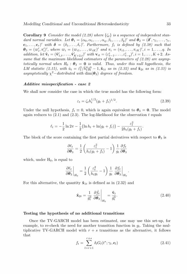
Modelling Conditional and Unconditional Heteroskedasticity 33
Corollary 9 Consider the model (2.28) where {ζt} is a sequence of independent stan-dard normal variables. Let θ1 = (α0, α1, . . . , αq, β1, . . . , βp)′ and θ2 = (δ′, γ1, . . . , γr,c1, . . . , cr)′ with δ = (δ1, . . . , δr)′. Furthermore, ft is defined by (2.38) such thatθ3 = ($′i, π
′i)′, where $i = ($i1, . . . , $iK)′ and πi = (πi1, . . . , πiK)′, i = 1, . . . , q. In
addition, let vt = (v′1,t, . . . , v′K+2,t)
′ with vit = (εit−1, . . . , εit−q)
′, i = 1, . . . ,K+2. As-sume that the maximum likelihood estimators of the parameters of (2.28) are asymp-totically normal when H0 : θ3 = 0 is valid. Thus, under this null hypothesis, theLM statistic (2.15), with ut = ε2t/h
0t g
0t − 1, x1t as in (2.32) and x2t as in (2.33) is
asymptotically χ2−distributed with dim(θ3) degrees of freedom.
Additive misspecification - case 2
We shall now consider the case in which the true model has the following form:
εt = ζth1/2t (gt + ft)1/2. (2.39)
Under the null hypothesis, ft ≡ 0, which is again equivalent to θ3 = 0. The modelagain reduces to (2.1) and (2.3). The log-likelihood for the observation t equals
`t = −12
ln 2π − 12{lnht + ln(gt + ft)} −
ε2t2ht(gt + ft)
.
The block of the score containing the first partial derivatives with respect to θ3 is
∂`t∂θ3
=12
(ε2t
ht(gt + ft)− 1)
1gt
∂ft∂θ3
which, under H0, is equal to
∂`t∂θ3
∣∣∣∣H0
=12
(ε2thtgt
− 1)
1gt
∂ft∂θ3
∣∣∣∣H0
.
For this alternative, the quantity x1t is defined as in (2.32) and
x2t =1g0t
∂ft∂θ3
∣∣∣∣∣H0
=vtg0t
. (2.40)
Testing the hypothesis of no additional transitions
Once the TV-GARCH model has been estimated, one may use this set-up, forexample, to re-check the need for another transition function in gt. Taking the mul-tiplicative TV-GARCH model with r + s transitions as the alternative, it followsthat
ft =r+s∑l=r+1
δlGl(t∗; γl, cl) (2.41)

34 Chapter 2
The hypothesis of no additional transitions is H0 : γr+1 = ... = γr+s = 0. Under thishypothesis, the parameters (δl, c′l)
′ are not identified. To circumvent this problem, wereplace the transition function Gl(t∗; γl, cl) by its first-order Taylor expansion aroundγl = 0, l = r + 1, . . . , r + s. After merging terms, we obtain
gt + ft = 1 +r∑l=1
δlGl(t∗; γl, cl) +r+s∑l=r+1
δl(γlc0 +K∑k=1
γlck(t∗)k) +R∗6
= δ∗l +r∑l=1
δlGl(t∗; γl, cl) +r+s∑l=r+1
K∑k=1
ψlk(t∗)k +R∗6 (2.42)
where δ∗l = 1 +∑r+sl=r+1 γlδlc0 and ψlk = γlδlck, l = r+ 1, . . . , r+ s, k = 1, . . . ,K. It is
convenient to reparameterize (2.41) as follows:
ft =r+s∑l=r+1
K∑k=1
ψlk(t∗)k +R∗6 (2.43)
Under the null hypothesis, the remainder R∗6 vanishes. It seems that the coefficientsψlk, l = r + 1, . . . , s, for a fixed k, are not identified because they are all related tothe same variable (t∗)k. They have to be merged, which leads to
ft =K∑k=1
ψ∗k(t∗)k +R∗6.
In other words, the test statistic is the same, independent of whether we would betesting against including Gr+1 or including Gr+1, . . . , Gr+s, s ≥ 2. Compare this withCorollary 5, which is a special case. In fact, Corollary 5 contains another example ofa misspecification test of the multiplicative model in which the misspecification is ofthe type ht(gt + ft).
Multiplicative misspecification
Under multiplicative misspecification, the parametric alternative to the TV-GARCHmodel is formulated as
εt = ζt(htgtft)1/2. (2.44)
In this framework, H0 : ft ≡ 1, which is equivalent to θ3 = 0. Under the nullhypothesis, the model reduces to the multiplicative TV-GARCH model. For thisspecification, the log-likelihood function for observation t may be written
`t = −12
ln 2π − 12
(lnht + ln gt + ln ft)−ε2t
2htgtft.
The additional block of the score has the form
∂`t∂θ3
=12
(ε2t
htgtft− 1)∂ft∂θ3

Modelling Conditional and Unconditional Heteroskedasticity 35
which, under H0, reduces to
∂`t∂θ3
∣∣∣∣H0
=12
(ε2thtgt
− 1)∂ft∂θ3
∣∣∣∣H0
.
Taking (2.44) as the alternative, the vector x1t is given in (2.32) and
x2t =∂ft∂θ3
∣∣∣∣∣H0
= vt. (2.45)
This category includes general misspecification tests of adequacy of the estimatedspecification. After the estimation of the TV-GARCH model, one may want tocheck whether the estimated standardized errors still contain some structure. In theGARCH context, Lundbergh and Terasvirta (2002) proposed a Lagrange multiplierstatistic for testing the hypothesis of no remaining ARCH which is asymptoticallyequivalent to the portmanteau statistic introduced by Li and Mak (1994). A similartest statistic can be obtained for the multiplicative TV-GARCH model.
Testing the hypothesis of no remaining ARCH
An important misspecification test for the multiplicative TV-GARCH specificationis the so-called ’ARCH-in-GARCH’ test. The original model
εt = ζth1/2t g
1/2t , ζt ∼ nid(0, 1)
is extended by assuming that, under the alternative, ζt = ξtf1/2t , where ξt ∼ nid(0, 1),
and
ft = 1 +s∑j=1
φjζ2t−j . (2.46)
The hypothesis of interest is H0 : φ1 = ... = φs = 0 and ∂ft
∂θ3|H0 = (ζ2
1 , . . . , ζ2s )′. Some
special cases may be mentioned. If gt ≡ 1, the test collapses into the test of ’noARCH-in-GARCH’ in Lundbergh and Terasvirta (2002). If ht ≡ 1 as well, the testcoincides with the Engle’s test of no ARCH. Setting only ht ≡ 1, it reduces to thetest of no ARCH in εt/g
1/2t . The test is presented in the next corollary.
Corollary 10 Consider the model (2.44) where {ζt} is a sequence of independentstandard normal variables. Let θ1 = (α0, α1, . . . , αq, β1, . . . , βp)′ and θ2 = (δ′, γ1, . . . ,γr, c1, . . . , cr)′ with δ = (δ1, . . . , δr)′. Furthermore, ft is defined by (2.46) such thatθ3 = (φ1, . . . , φs)′ and vt = (ζ2
1 , . . . , ζ2s )′. Assume that the maximum likelihood estima-
tors of the parameters of (2.44) are asymptotically normal when H0 : θ3 = 0 is valid.Thus, under this null hypothesis, the LM statistic (2.15), with ut = ε2t/h
0t g
0t − 1, x1t
as in (2.32) and x2t = vt is asymptotically χ2−distributed with s degrees of freedom.
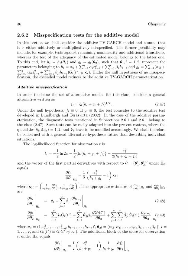
36 Chapter 2
2.6.2 Misspecification tests for the additive model
In this section we shall consider the additive TV-GARCH model and assume thatit is either additively or multiplicatively misspecified. The former possibility mayinclude, for example, tests against remaining nonlinearity and additional transitions,whereas the test of the adequacy of the estimated model belongs to the latter one.To this end, let ht = ht(θ1) and gt = gt(θ2), such that θi, i = 1, 2, represent theparameters belonging to ht = α0 +
∑qi=1 αiε
2t−i +
∑pj=1 βjht−j and gt =
∑rl=1(α0l +∑q
i=1 αilε2t−i +
∑pj=1 βjlht−j)Gl(t
∗; γl, cl). Under the null hypothesis of no misspeci-fication, the extended model reduces to the additive TV-GARCH parameterization.
Additive misspecification
In order to define the set of alternative models for this class, consider a generalalternative written as
εt = ζt(ht + gt + ft)1/2. (2.47)
Under the null hypothesis, ft ≡ 0. If gt ≡ 0, the test coincides to the additive testdeveloped in Lundbergh and Terasvirta (2002). In the case of the additive param-eterization, the diagnostic tests mentioned in Subsections 2.6.1 and 2.6.1 belong tothe class (2.47). Such tests can be easily adapted into the present context, where thequantities ut, xit, i = 1, 2, and vt have to be modified accordingly. We shall thereforebe concerned with a general alternative hypothesis rather than describing individualsituations.
The log-likelihood function for observation t is
`t = −12
ln 2π − 12{ln(ht + gt + ft)} −
ε2t2(ht + gt + ft)
and the vector of the first partial derivatives with respect to θ = (θ′1,θ′2)′ under H0
equals∂`t∂θ
∣∣∣∣H0
=12
(ε2t
ht + gt− 1)
x1t
where x1t =(
1ht+gt
∂ht
∂θ′1, 1ht+gt
∂gt
∂θ′2
)′. The appropriate estimates of ∂ht
∂θ1|H0 and ∂gt
∂θ2|H0
are
∂ht∂θ1
∣∣∣∣∣H0
= zt +p∑j=1
βj∂ht−j∂θ1
∣∣∣∣∣H0
(2.48)
∂gt∂θ2
∣∣∣∣H0
=r∑l=1
ztGl(t∗) +r∑l=1
θ′2lzt
∂Gl(t∗)∂θ2
+p∑j=1
r∑l=1
βjlGl(t∗)∂gt−j∂θ2
∣∣∣∣H0
(2.49)
where zt = (1, ε2t−1, . . . , ε2t−q, ht−1, . . . , ht−p)′,θ2l = (α0l, α1l, . . . , αql, β1l, . . . , βpl)′, l =
1, . . . , r, and Gl(t∗) ≡ Gl(t∗; γl, cl). The additional block of the score for observationt, under H0, equals
∂`t∂θ3
∣∣∣∣H0
=12
(ε2t
ht + gt− 1)
1ht + gt
∂ft∂θ3
∣∣∣∣H0

Modelling Conditional and Unconditional Heteroskedasticity 37
where ∂ft
∂θ3= vt. To define the LM statistic, set
x1t =
(1
h0t + g0
t
∂ht
∂θ′1
∣∣∣∣∣H0
,1
h0t + g0
t
∂gt
∂θ′2
∣∣∣∣H0
)′(2.50)
x2t =1
h0t + g0
t
∂ft∂θ3
∣∣∣∣∣H0
=vt
h0t + g0
t
(2.51)
where ∂ht
∂θ1|H0 and ∂gt
∂θ2|H0 are given in (2.48) and (2.49), respectively. These results
apply to the test against remaining nonlinearity. The test will be presented in thefollowing corollary.
Corollary 11 Consider the model (2.47) where {ζt} is a sequence of independentstandard normal variables. Let θ1 = (α0, α1, . . . , αq, β1, . . . , βp)′,θ2 = (δ′, γ1, . . . , γr,c1, . . . , cr)′ with δ = (δ1, . . . , δr)′ and θ3 = ($′i, π
′i)′, where $i = ($i1, . . . , $iK)′
and πi = (πi1, . . . , πiK)′, i = 1, . . . , q. Assume that the maximum likelihood estima-tors of the parameters of (2.47) are asymptotically normal when H0 : θ3 = 0 isvalid. Thus, under this null hypothesis, the LM statistic (2.15), with ut = ε2t/(h
0t +
g0t ) − 1, x1t as in (2.50) and x2t as in (2.51) with vt = (v′1,t, . . . , v
′K+2,t)
′ wherevit = (εit−1, . . . , ε
it−q)
′, i = 1, . . . ,K+2, is asymptotically χ2−distributed with dim(θ3)degrees of freedom.
Multiplicative misspecification
Consider the following extended TV-GARCH model
εt = ζt(ht + gt)1/2f1/2t . (2.52)
Under the null hypothesis, ft ≡ 1. This category entails the test for assessing theadequacy of the functional form of the estimated model. This test was already dis-cussed when the TV-GARCH model was in the multiplicative form and the sameconsiderations apply here.
The log-likelihood function for a single observation on (2.52) is
`t = −12
ln 2π − 12{ln(ht + gt) + ln ft)} −
ε2t2(ht + gt)ft
and the relevant block of the score due to θ3, under H0, has the form
∂`t∂θ3
∣∣∣∣H0
=12
(ε2t
ht + gt− 1)∂ft∂θ3
∣∣∣∣H0
.
The hypothesis of interest is that the squared standardized error sequence is iid.Under the alternative, ft is defined in (2.46). In this framework, the vector x1t isgiven as in (2.50) and x2t = ∂ft
∂θ3|H0 = vt. The following Corollary defines the test
statistic.

38 Chapter 2
Corollary 12 Consider the model (2.52) where {ζt} is a sequence of independentstandard normal variables. Let θ1 = (α0, α1, . . . , αq, β1, . . . , βp)′ and θ2 = (δ′, γ1, . . . ,γr, c1, . . . , cr)′ with δ = (δ1, . . . , δr)′. Furthermore, ft is defined by (2.46) such thatθ3 = (φ1, . . . , φs)′ and vt = (ζ2
1 , . . . , ζ2s )′. Assume that the maximum likelihood estima-
tors of the parameters of (2.52) are asymptotically normal when H0 : θ3 = 0 is valid.Thus, under this null hypothesis, the LM statistic (2.15), with ut = ε2t/(h
0t+g
0t )−1, x1t
as in (2.50) and x2t = vt is asymptotically χ2−distributed with s degrees of freedom.
2.7 Simulation study
2.7.1 Monte Carlo design
In this section, we conduct a small simulation experiment to evaluate the finite-sample properties of the proposed parameter constancy tests. These are the testsagainst an additive and a multiplicative TV-GARCH specifications. Specifically, weshall investigate the size and power properties of the LM-type tests involved in themodelling strategies as well as the success rate of the specification procedures. Samplelengths of 1000, 2500 and 5000 observations have been used in all simulations. Foreach design, the total number of replications equals 2000. To avoid the initializationeffects, the first 1000 observations have been discarded before generating the actualseries. All the computations have been carried out using Ox, version 3.30 (see Doornik(2002)). The behaviour of the test statistics is examined for several data generatingprocesses (DGP’s) that can be nested in the following TV-GARCH specification:
yt = εt, εt|Ft−1 ∼ N(0, ht)ht = α0 + α1ε
2t−1 + β1ht−1 + (α01 + α11ε
2t−1 + β11ht−1)G1(t∗; γ1, c1). (2.53)
The data generating processes are as following:
DGP (i):ht = 0.10 + α1ε
2t−1 + β1ht−1
α1 = {0.05, 0.09, 0.10} and β1 = {0.80, 0.85, 0.90}
DGP (ii):ht = 0.10 + α01G1(t∗; γ1, c1) + 0.10ε2t−1 + 0.80ht−1
α01 = {0.10, 0.30}
DGP (iii):ht = 0.10 + (0.10 + α11G1(t∗; γ1, c1))ε2t−1 + 0.80ht−1
α11 = {0.05, 0.09}

Modelling Conditional and Unconditional Heteroskedasticity 39
DGP (iv):ht = (0.10 + α01G1(t∗; γ1, c1)) + (0.10 + α11G1(t∗; γ1, c1))ε2t−1 + 0.80ht−1
α01 = {0.10, 0.30} and α11 = {0.05, 0.09}
DGP (v):ht = 0.10 + 0.10ε2t−1 + (0.80 + β11G1(t∗; γ1, c1))ht−1
β11 = {0.05, 0.09}
DGP (vi):ht = 0.10 + α01G1(t∗; γ1, c1) + 0.10ε2t−1 + (0.80 + β11G1(t∗; γ1, c1))ht−1
α01 = {0.10, 0.30} and β11 = {0.05, 0.09}
DGP (vii):ht = (0.10 + 0.10ε2t−1 + 0.85ht−1)(1 + δ1G1(t∗; γ1, c1))δ1 = {0.05, 0.08}
The first six designs concern the additive TV-GARCH model, whereas the re-maining one relates to the multiplicative model. In all these seven experiments, themidpoint of the change in volatility is at c1 = 0.5, whereas the slope parameter γ1
varies in the interval γ1 = {5, 10}. Following the suggestion in Bollerslev (1986), re-cursive computation of ht is initialized by using the estimated unconditional variancefor the pre-sample values t ≤ 0.
2.7.2 Finite sample properties
In this section we shall look at the small-sample properties of the modelling strategyfor the TV-GARCH model. We first report results on the size and power propertiesof our parameter constancy tests. Then we turn to the specification of TV-GARCHmodels.
Size and power simulations
The size and the power results of the tests are presented in graphs following therecommendation by Davidson and MacKinnon (1998). Both the ordinary and therobustified versions of each test are computed using auxiliary regressions. Results ofthe size simulations appear in the form of p-value discrepancy plots in Figure 2.5. Inthese graphs, the difference between the empirical size and the nominal size is plottedagainst the nominal size. The upper panel of Figure 2.5 presents the results for thesize simulations for the test against an additive alternative, whereas the bottom panelshows the empirical size results of the test against a multiplicative alternative. Foreach test we calculate the actual rejection frequencies for the three sample sizes at thefollowing nominal levels: 0.1%, 0.3%, 0.5%, 0.7%, 0.9%, 1%, ...., 10%. The series are

40 Chapter 2
0.00 0.01 0.02 0.03 0.04 0.05 0.06 0.07 0.08 0.09 0.10−0.08
−0.06
−0.04
−0.02
0.00
0.02
0.04
0.06
0.08LM3_1000 LM3_2500 LM3_5000
0.00 0.01 0.02 0.03 0.04 0.05 0.06 0.07 0.08 0.09 0.10−0.08
−0.06
−0.04
−0.02
0.00
0.02
0.04
0.06
0.08LM3rob_1000 LM3rob_2500 LM3rob_5000
0.00 0.01 0.02 0.03 0.04 0.05 0.06 0.07 0.08 0.09 0.10−0.08
−0.06
−0.04
−0.02
0.00
0.02
0.04
0.06
0.08LM3_1000 LM3_5000 LM3_2500
0.00 0.01 0.02 0.03 0.04 0.05 0.06 0.07 0.08 0.09 0.10−0.08
−0.06
−0.04
−0.02
0.00
0.02
0.04
0.06
0.08LM3rob_1000 LM3rob_2500 LM3rob_5000
Figure 2.5 Size discrepancy plots of the additive (upper panel) and multiplicative(lower panel) parameter constancy tests. Both the ordinary (left) and the robust(right) versions of the tests are plotted.
generated from the GARCH model given by the DGP (i) where α0 = 0.10, α1 = 0.10and β1 = 0.85.
Both tests are somewhat size-distorted at the sample size T = 1000, but the resultsbecome more accurate as the sample size increases. For sample sizes typically usedfor modelling volatility clustering, such as T = 2500 and T = 5000, the tests arereasonably well-sized. Furthermore, the size distortions in the robust version of thetests do not differ too much from those in the non-robust test. Our main conclusionis that both the non-robust and robust versions of the test statistics are rather goodapproximations to the finite-sample distributions for T ≥ 2500. Employing a robusttest even when the errors are normal does not seem to lead to a large loss of power.
Although there exist several parameter constancy tests in the GARCH literature,none of them can be considered a direct benchmark for our parameter constancy tests.Because of this, in Figure 2.6 we only report power results for our tests. In thesegraphs the rejection frequencies are plotted against the nominal significance levels0.1%, 0.3%, 0.5%, 0.7%, 0.9%, 1%, . . ., 10%. Instead of the size-adjusted power-sizecurves suggested by Davidson and MacKinnon (1998), we simply report power curvesas the tests have good size properties.
The power results in Figure 2.6 have been obtained by generating artificial data

Modelling Conditional and Unconditional Heteroskedasticity 41
0.00 0.01 0.02 0.03 0.04 0.05 0.06 0.07 0.08 0.09 0.10
0.2
0.4
0.6
0.8
1.0
LM3_1000 LM3_2500 LM3_5000
0.00 0.01 0.02 0.03 0.04 0.05 0.06 0.07 0.08 0.09 0.10
0.2
0.4
0.6
0.8
1.0
LM3rob_1000 LM3rob_2500 LM3rob_5000
0.00 0.01 0.02 0.03 0.04 0.05 0.06 0.07 0.08 0.09 0.10
0.2
0.4
0.6
0.8
1.0
LM3_1000 LM3_2500 LM3_5000
0.00 0.01 0.02 0.03 0.04 0.05 0.06 0.07 0.08 0.09 0.10
0.2
0.4
0.6
0.8
1.0
LM3rob_1000 LM3rob_2500 LM3rob_5000
Figure 2.6 Power curves of the additive (upper panel) and multiplicative (lowerpanel) parameter constancy tests. Both the ordinary (left) and robust (right) versionsof the tests are plotted.
from the DGP (ii) where the coefficient α01 = 0.10, the slope parameter γ1 = 5 andthe location parameter c1 = 0.5. The rejection frequencies of the additive LM teststatistics shown in the top panel are moderate when T = 1000 and increase with thesample size. The pattern of the power results for the robustified version of the test isvery similar to the non-robust one.
Rejection frequencies for the LM-type test against a multiplicative alternative areshown in the lower panel of Figure 2.6. The results refer to power simulations whenthe data generating process is a multiplicative TV-GARCH model (DGP vii). Thecoefficient δ1 = 0.05 and γ1 = 5 as before. As expected, the rejection frequencies arean increasing function of the sample size and of the parameter δ1 (as well as of theparameter α01 in the additive case). Moreover, the LM-type test statistic turns outto be very powerful even for short time series. Again, the behaviour of the robustversion of the test in the power simulations is quite similar to that of the non-robustversion.
Simulating the model selection strategy
In this section we consider the performance of the specific-to-general specificationstrategy for TV-GARCH models with an additive time-varying structure. This is done

42 Chapter 2
by studying the selection frequencies of various models. The specification procedurehas been discussed in Section 2.4.1. A total of 2000 replications are carried out for eachDGP and all three sample sizes. The first 1000 observations of each generated seriesare discarded to avoid the initialization effects. Throughout, we set α = 0.05 for boththe LM1 and LM3 versions of the test. The maximum number of transitions consideredequals two. Furthermore, τ = 1/2, which means that we halve the significance levelof the test at each stage of the sequence.
Results for DGP (i) are reported in Table 2.1 (see Appendix B). The frequencies ofthe correct number of transitions are shown in boldface. The column labelled ‘choice’refers to the number of transition functions selected. In general, the statistic LM1
has better size properties than LM3. However, in most cases, the test based on thethird-order Taylor expansion also has an empirical size very close to the nominal sizeexcept when the sum α1 + β1 is close to one and the sample size is less than 2500observations.
Results for series generated from a model with a single transition function can befound in Table 2.2. We report separately an additive time-varying structure in eachparameter of the GARCH model when c1 = 0.50. This corresponds to the DGP’s(ii), (iii) and (v). For all the cases, the parameters of the linear GARCH are α0 =0.10, α1 = 0.10 and β1 = 0.80. Clearly, the constant-parameter GARCH model ischosen too often for parameterizations with smoothest changes and shortest series.For large sample sizes, the selection frequencies of the true model become quite higheven for very smooth changes. Again, the LM1-test has higher power than LM3. Asexpected, the correct model is selected more frequently for high than for low values ofα01, α11 or β11. Moreover, the correct model is selected slightly more often when thechange only occurs either in the constant α0 or in the GARCH parameter β1 thanwhen it does in the ARCH parameter α1.
The model selection frequencies when the series are generated from DGP (iv) aregiven in Table 2.3. The correct model is chosen more frequently when the change inα01 and α11 becomes large. It also becomes easier to identify a single transition whenthe slope parameter γ increases. Again, the results concern the case when the changeoccurs in the middle of the sample. Finally, Table 2.4 contains the frequencies of theselected models for the DGP (vi). In this case, the power of our procedure turns outto be very similar to that shown in Table 2.3. This may be explained by the factthat either changes in α01 and α11 or the ones in α01 and β11 simultaneously changethe amplitude of clusters as well as the unconditional variance. We also carried outsimulations for the DGP (vii) which are not reported in the paper. The results arealmost identical to what is reported for the additive TV-GARCH model. Overall, thesequential procedure seems to work relatively well for all combinations of parametersconsidered and for sample sizes T ≥ 1000.
2.8 Applications
In this section we shall present two empirical examples involving two financial timeseries, a stock index and an exchange rate return series. The former is the Standard

Modelling Conditional and Unconditional Heteroskedasticity 43
0 250 500 750 1000 1250 1500 1750 2000 2250 2500
−6
−4
−2
0
2
4
6
Figure 2.7 Daily returns of the S&P 500 composite index from January 2, 1990until December 31, 1999 (2531 observations).
and Poor 500 composite index (S&P 500) and the latter the spot exchange rate ofthe Singapore dollar versus the U.S. dollar (SPD/USD). Both series are observed ata daily frequency and transformed into the continuously compounded rates of return.
2.8.1 Stock index returns
The daily S&P 500 return series was provided by the Yahoo-Quotes database. Thesample extends from January 2, 1990, to December 31, 1999, which amounts to 2531observations. The series is plotted in Figure 2.7. It contains periods of large volatilityboth in the beginning and at the end of the sample period, whereas the averagevolatility in the middle of the sample is somewhat lower than in both ends.
Summary statistics for the series can be found in the second column of Table 2.5.It is seen that there is both negative skewness and excess kurtosis in the series.Normality of the marginal distribution of the S&P 500 returns is strongly rejected.Robust skewness and kurtosis estimates (see Kim and White (2004) and Terasvirtaand Zhao (2007)) are also provided. The robust skewness measure is positive but veryclose to zero, which suggests that the asymmetry of the empirical distribution of thereturns is due to a small number of outliers. The robust centred kurtosis that hasvalue zero for the normal distribution indicates some excess kurtosis but much lessthan the conventional measure. This is in line with the robust skewness estimate. As

44 Chapter 2
expected, the null hypothesis of no ARCH is strongly rejected.We first estimate a standard GARCH(1,1) model to this series. In order to save
space, the results are not shown here. Results of the parameter constancy test againstan additive time-varying structure are reported in Table 2.7. The test of parameterconstancy against an additive TV-GARCH model, when several parameters are as-sumed to change under the alternative, rejects the null hypothesis. The tests againstalternatives in which some parameters remain constant, suggest that the the interceptmay be the main source of nonconstancy.
Instead of specifying and estimating an additive TV-GARCH model with a time-varying intercept, we test the iid hypothesis of our stochastic sequence {εt} againstdeterministic change. This is Step 1 in the specification of multiplicative TV-GARCHmodels outlined in Subsection 2.4.2. The results can be found in Table 2.8. Thenull hypothesis is rejected very strongly as the p-value of the test equals 3 × 10⁻²³.The test sequence for specifying the structure of the deterministic function gt pointstowards K = 2. Fitting the TV-GARCH model with a single transition function andK = 2 to the series and testing for another transition still leads to rejecting the nullhypothesis. The p-value, however, is now considerably larger, equalling 0.0028, andthe specification test sequence now clearly suggests K = 1. Accepting this outcome,fitting the corresponding TV-GARCH model to the series and testing for yet anothertransition yields the p-value 0.0623. If the null hypothesis is tested directly against astandard logistic transition function, the p-value equals 0.0197. Given the relativelylarge number of observations, this is not a small value, and the model with twotransitions is tentatively accepted as the final model.
In this model, the estimate of gt has the following form:
gt = {1 + 1.7041(0.4265)
G1(t∗; γ1, c1) + 1.7335(0.5455)
G2(t∗; γ2, c2)} (2.54)
withG1(t∗; γ1, c1) = (1 + exp{−100
(−)(t∗ − 0.1643
(0.0100))(t∗ − 0.6950
(0.0831))})−1 (2.55)
andG2(t∗; γ2, c2) = (1 + exp{−100
(−)(t∗ − 0.8534
(0.0043))})−1. (2.56)
The graph of the deterministic component gt is depicted in Figure 2.9. The twotransitions are clearly visible and illustrate how volatility first decreases and thenincreases over time. A GARCH model is fitted to the standardized residuals εt/g
1/2t ,
and the estimated model is subjected to misspecification tests described in Subsection2.6.1. Table 2.9 contains the test results. The hypothesis of ’no ARCH in GARCH’is not rejected for any lag length considered. As may be expected, the hypothesis ofno additional transitions is not rejected either. There is, however, some indication ofnonlinearity in the conditional variance as the GARCH(1,1) component is stronglyrejected against a STGARCH(1,1) one for K = 1. In order to remedy this problem,we specify a GJR-GARCH(1,1) model for ht.
The parameter estimates of the GJR-GARCH model can be found in Table 2.6. Itis seen that the persistence factor equals α1 + β1 + γ1/2 = 0.993, so that the estimated

Modelling Conditional and Unconditional Heteroskedasticity 45
model is practically an integrated GJR-GARCH model. For illustration, Table 2.6also contains the parameter estimates at the point where the parameters in ht havebeen estimated for the first time. It is seen that there is already a large changein the value of the log-likelihood compared to the maximum found for the GJR-GARCH(1,1) model. The persistence, however, has not yet decreased very much.Figure 2.10 contains the autocorrelations of |εt| (Panel (a)) and those of |εt|/g1/2
t
after a single iteration (Panel (b)). It is seen that the increase in the log-likelihoodis mainly due to a decrease in the general level of the autocorrelations. At the sametime, the autocorrelations retain the ’long-memory property’, the very slow decay asa function of the lag, that is obvious in the autocorrelations of |εt|.
The log-likelihood considerably increases with further iterations, and the finalpersistence indicator has the remarkably low value α1 + β1 + γ1/2 = 0.918. A cleartrade-off is observed here. When it is assumed that the process is stationary there isonly one level (unconditional variance) to which the conditional variance convergeswhen it is assumed that zt = 0 for t > t0. This convergence then takes a very longtime (α1 + β1 + γ1/2 = 0.993 is very close to unity). In the TV-GJR-GARCH modelthis level is time-varying, and the rate of convergence to a particular level can thusbe much more rapid than it is in the standard GJR-GARCH model. Panel (c) ofFigure 2.10 now shows that the autocorrelations of |εt|/g1/2
t have decreased evenfurther, and only few of them exceed two standard deviations of |εt| under the iidnormality assumption, marked by the straight line in the figure. A major part of thevariation in the daily S&P 500 return series can thus be attributed to the slow-movingcomponent gt, and surprisingly little remains to be explained by the traditional GJR-GARCH component.
Table 2.10 contains the misspecification test results for this model. Even if theGJR-GARCH model is a rather crude representation of asymmetry compared to thesmooth transition GARCH specification, it manages to capture most of the asym-metry. The p-value of the test of no additional nonlinearity, when applied to theTV-GJR-GARCH model, equals 0.024, which is much larger than 1× 10⁻¹⁰ obtainedwhen the test was applied to the estimated TV-GARCH(1,1) model. Applying the1% significance level, the other misspecification tests do not reject the model either,and the TV-GJR-GARCH model is thus accepted to be our final model.
Figure 2.11 that contains the estimated conditional standard deviations h1/2t of
{εt} for the GJR-GARCH(1,1) model and the ones of {εt/g1/2t } illustrates the sit-
uation as well. For the GJR-GARCH model, see Panel (a), the graph looks rather’nonstationary’. Some nonstationarity remains after a single iteration, as the autocor-relations of {εt/g1/2
t } in Panel (b) also demonstrate. From the graph in Panel (c) (thefinal model) it is seen that volatility is still changing over time, but there no longerseem to be persistent level changes. They have been absorbed by the deterministiccomponent.
Column 4 in Table 2.5 contains the skewness and kurtosis estimates for εt/g1/2t .
The negative skewness remains but, as can be expected from the other results, theexcess kurtosis of the final εt/g
1/2t series is considerably less (2.8) than the original
number (5.3). This is another illustration of the fact that volatility to be modelled by

46 Chapter 2
ht in the TV-GJR-GARCH model is much smaller than it is in the GJR-GARCH(1,1)model without the nonstationary component. Even the robust kurtosis estimate inTable 2.5 shows some decrease, but because its nonrobust value was already small,the decrease has remained rather modest.
In Figure 2.12, the estimated news impact curve of the standard GJR-GARCH(1,1)model is compared with corresponding curves of the TV-GJR-GARCH(1,1) model.The news impact curve of the TV-GJR-GARCH model is time-varying because it de-pends on gt−1. The news impact curve of the GJR-GARCH model is time-invariant,and from the figure it is seen how the curve can vary over time in the TV-GJR-GARCH model. This curve is completely flat for εt−1 > 0 because α1 = 0 in themodel. Its estimate was originally slightly negative but statistically insignificant, andthe model was re-estimated after restricting α1 to zero. The curves based on theTV-GJR-GARCH model clearly show the obvious fact that when there is plenty ofturbulence in the market, the news impact of a particular negative shock is smallerthan it is when calm prevails. In the latter case, even a minor piece of ’bad news’(a negative shock) can be ’news’, whereas in the former case, even a relatively largenegative shock can have a rather small news component. This distinction cannotbe made in the standard GJR-GARCH model. According to our TV-GJR-GARCHmodel, ’good news’ (positive shocks) have no impact on volatility in this application.
2.8.2 Exchange rate data
The data of this section consist of daily returns of the spot SPD/USD exchange rateprovided by the Federal Reserve Bank of New York. The time series is shown inFigure 2.8. It covers the period from May 1, 1997 until July 11, 2005, yielding a totalof 2060 observations. At first sight, it appears that one can distinguish two differentregimes in the series. A period of high volatility occurs during the East Asian financialcrisis due to the significant depreciation of the Singapore dollar relative to the U.S.dollar. After the crisis, the volatility of the currency returns descends to a low level.
Descriptive statistics for the SPD/USD exchange rate returns are reported inTable 2.5. There is plenty of excess kurtosis, and the estimated skewness is stronglynegative. These values are due to a limited number of large negative returns earlyin the series during the so-called Asian crisis. Naturally, the marginal distribution ofthe returns is far from normal. The robust measure of skewness indicates that thereis in fact little skewness and the robust centred kurtosis is substantially smaller thanits standard measure. The hypothesis of no ARCH is strongly rejected, as can beexpected. The GARCH(1,1) model fitted to this exchange rate return series againshows high persistence of volatility. The estimate of α1 is larger and that of β1 smallerthan in the S&P 500 model, which is a consequence of the fact that the kurtosis islarger in the exchange rate series than it is in the S&P 500 returns.
Parameter constancy of the GARCH(1,1) model is rejected against an additive TV-GARCH model. These test results are presented in Table 2.7. In this case, however,the rejection is not due to the intercept but rather to the other two parameters.As in the previous application, we shall not fit any additive TV-GARCH modelsto our return series but choose to work with the multiplicative model. The test of

Modelling Conditional and Unconditional Heteroskedasticity 47
0 300 600 900 1200 1500 1800 2100−4
−3
−2
−1
0
1
2
3
Figure 2.8 Daily returns of the Singapore Dollar versus US dollar exchange ratefrom May 1, 1997 until July 11, 2005 (2060 observations).
constant unconditional variance against a time-varying one has the p-value equal to1 × 10−20. Table 2.8 contains the outcomes of the sequence of specification tests.The results indicate that one should choose K = 1, that is, have a monotonicallyincreasing transition function. A multiplicative TV-GARCH model with a singletransition appears adequate in the sense that the test for another transition hasp = 0.14. The diagnostic tests of this model in Table 2.9 do not reject the model.There is no remaining ARCH in the standardized errors, no evidence of higher-orderstructure in the GARCH component, and nothing suggests the existence of additionaltransitions. Finally, the linearity test against the smooth transition GARCH doesnot indicate remaining nonlinearity. Judging from these statistics, the model seemsto be adequately specified. It is thus tentatively accepted as our final model for theSPD/USD daily return series.
The final estimates for the function gt are as follows:
gt = {1− 0.7890(0.0074)
G1(t∗; γ1, c1)}, (2.57)
whereG1(t∗; γ1, c1) = (1 + exp{−100
(−)(t∗ − 0.2101
(0.0014))})−1 (2.58)
The graph of the transition function can be found in Figure 2.13. Figure 2.8 already

48 Chapter 2
shows that the volatility is high in the beginning and settles down to a lower levelafter about 500 observations (two years). From Table 2.5 it is seen that the excesskurtosis has decreased substantially from its value for {εt} and, furthermore, thatthe skewness has been reduced from −0.9 to less than −0.3. This large reductioncan be ascribed to the fact that the original skewness was due to a couple of verylarge negative returns during the Asian crisis. Their significance has subsequentlybeen reduced in {εt/g1/2
t } where the conditional heteroskedasticity component hasbeen standardized by the underlying nonstationary volatility component. Besides,according to the robust estimates the skewness has not been affected, which is in linewith this conclusion as well.
The parameter estimates of the model appear in Table 2.6. It can be seen thateven for the exchange rate series, the first iteration already has a large effect on thevalue of the log-likelihood. Figure 2.14 shows that at that stage, the autocorrelationsof |εt|/g1/2
t are considerably lower than those of |εt|, although their decay as a functionof the lag length is still slow. The final estimates indicate more persistence than thereis in the S&P 500 case, but the decrease is still large compared to the GARCH(1,1)model. The decay rate of the autocorrelations of |εt|/g1/2
t in Figure 2.14 is quite rapidand looks more or less exponential. The first-order autocorrelation that was about0.304 for |εt| equals 0.121 for |εt|/g1/2
t . The graph of the conditional variance ht inPanel (a) of Figure 2.15 clearly shows the period of high volatility, which is the causeof the high persistence suggested by the GARCH(1,1) model. Panel (c) shows that inthe final model this high-volatility period is explained by the deterministic componentgt, and that the graph of ht does not show signs of nonstationarity. This is preciselywhat one would expect after a look at the parameter estimates in Table 2.6.
Figure 2.16 contains the estimated news impact curves of the traditional GARCH(1,1)model and the ones of the TV-GARCH(1,1) model for three regimes. It is seen thatsymmetry in the response of volatility to news is preserved in the latter model. This isobviously because of certain ’symmetry’ of the exchange rates: good news for the USdollar may be bad news for the SPD, and vice versa. An additional result, similarlyto the previous application, is the ability of the time-varying news impact curves todistinguish different reaction levels of volatility to news in calm and turbulent times.In general, the impact of news on volatility tends to be high in expansions and low inrecessions.
2.9 Concluding remarks
In this paper we introduce two new nonstationary GARCH models whose parame-ters are allowed to have a smoothly time-varying structure. Time-variation of the(un)conditional variance is incorporated in the model either in an additive or a mul-tiplicative form. This approach is appealing since most daily financial return seriescover a long time period and non-constancy of parameters in models describing themtherefore appears quite likely. We also develop a modelling strategy for our TV-GARCH specifications. In order to determine the appropriate number of transitionswe propose a procedure consisting of a sequence of Lagrange multiplier tests. The

Modelling Conditional and Unconditional Heteroskedasticity 49
test statistics can be robustified against deviations from the iid assumption. Oursimulation experiments suggest that the parameter constancy tests have reasonablegood properties already in samples of moderate size. The modelling strategy appearsto work quite well for the data-generating processes that we simulate.
We put our TV-GARCH models to test by applying the modelling strategy todaily stock index and exchange rate returns. We find that parameter constancyagainst an additive and a multiplicative structure is strongly rejected for both returnseries. Fitting a traditional GARCH model to these series yields results that arequite different from the ones obtained by our approach and suggest the presence oflong memory in volatility. Our results show that the long-memory type behaviour ofthe sample autocorrelation functions of the absolute returns may also be induced bychanges in the unconditional variance. Once the model accounts for the time-variationin the baseline volatility or unconditional variance, the evidence for long memory isconsiderably weakened or even vanishes altogether.
An extension to multivariate GARCH models appears possible. The so-calledConstant Conditional Correlation (CCC-) GARCH model by Bollerslev (1990) andits extensions typically make use of a standard GARCH(1,1) specification for condi-tional variances. These GARCH equations could be generalized to account for time-variation in parameters. An interesting question to investigate with our TV-GARCHspecifications is how such a generalization would affect estimates of time-varying cor-relations in a situation in which there are changes in the unconditional variance ofthe return series. This and other extensions to multivariate models will be left forfuture work.

50 Chapter 2
Appendix A: Proof of Theorem 1
Proof of Theorem 1. Assuming the independent innovations to be normallydistributed, it follows that for model (2.11), the conditional log-likelihood function isgiven by
LT (θ) = −T2
ln 2π − 12
T∑t=1
lnht −12
T∑t=1
ε2tht.
Let θ be a parameter vector partitioned as θ = (θ′1,θ′2)′. The null hypothesis is
θ2 = 0. The corresponding partition of the average score vector q(T )(θ) is q(T )(θ) =(q1(T )(θ1)′,q2(T )(θ2)′)′. Let h0
t denote the conditional variance under the null hy-pothesis and let the true parameter vector under H0 be θ0 = (θ0′
1 ,0′)′. The Lagrange
multiplier statistic is defined as follows:
ξLM = Tq(T )(θ)′I(θ)−1q(T )(θ)
where T is the sample size, θ = (θ′1,0′)′ is the constrained maximum likelihood esti-
mator of θ,
q(T )(θ) = (0′,q2(T )(0)′)′ = (0′,1T
T∑t=1
∂`t(θ)∂θ′2
|H0)′
is the average score vector and I(θ) the information matrix, both evaluated at θ = θ.In this case, the partial derivatives with respect to θ have the form
∂`t(θ)∂θ
=12
(ε2tht− 1)
1ht
∂ht∂θ
=12
(ε2tht− 1)
xt
where xt = (x′1t,x′2t)′, with x1t = 1
ht
∂ht
∂θ1and x2t = 1
ht
∂ht
∂θ2. Accordingly,
q(T )(θ) =1
2T
T∑t=1
(ε2t
h0t
− 1
)xt =
(0′,
12T
T∑t=1
(ε2t
h0t
− 1
)x′2t
)′
where h0t and xt = (x′1t, x
′2t)′ denote h0
t and xt, respectively, evaluated at θ = θ. Under normality, the population information matrix equals the negative expectedvalue of the average Hessian matrix:
I(θ) = −E
[1T
T∑t=1
∂2`t(θ)∂θ∂θ′
].
The Hessian of the log-likelihood equals
T∑t=1
∂2`t(θ)∂θ∂θ′
= −12
T∑t=1
[ε2th3t
∂ht∂θ
∂ht
∂θ′+
1ht
(ε2tht− 1)(
∂2ht
∂θ∂θ′− 1ht
∂ht∂θ
∂ht
∂θ′
)]

Appendix A: Proof of Theorem 1 51
so the information matrix becomes
I(θ) =1
2T
T∑t=1
E
[ε2th3t
∂ht∂θ
∂ht
∂θ′
]=
12T
T∑t=1
Extx′t.
As the maximum likelihood estimator θ is consistent for θ0,
I(θ) =1
2T
T∑t=1
xtx′t
is consistent for I(θ). Then the Lagrange multiplier type test statistic for testingparameter constancy has the standard form:
ξLM =12
T∑t=1
utx′t
(T∑t=1
xtx′t
)−1 T∑t=1
xtut
=12
T∑t=1
utx′2t
T∑t=1
x2tx′2t −T∑t=1
x2tx′1t
(T∑t=1
x1tx′1t
)−1 T∑t=1
x1tx′2t
−1
T∑t=1
x2tut.
where ut = ε2t/h0t −1. Under H0 and standard regularity conditions, the statistic ξLM
has an asymptotic χ2-distribution with dim (θ2) degrees of freedom.

52 Chapter 2
Appendix B: Tables and Figures
Table 2.1 Model selection frequencies based on the additive sequential procedure
Number of T = 1000 T = 2500 T = 5000α1 β1 transitions LM1 LM3 LM1 LM3 LM1 LM3
DGP (i): GARCH model with α0 = 0.10
0.10 0.80 r = 0 95.45 94.15 95.00 95.35 95.50 94.35r = 1 3.36 4.10 3.90 3.05 3.30 3.90r ≥ 2 1.20 1.75 1.10 1.60 1.20 1.75
0.10 0.85 r = 0 94.70 91.90 94.30 94.10 95.10 93.70r = 1 3.65 5.20 4.60 3.90 3.40 4.45r ≥ 2 1.65 2.90 1.05 2.00 1.50 1.85
0.05 0.90 r = 0 94.45 90.45 94.20 93.75 94.40 93.25r = 1 4.00 6.35 4.50 4.20 4.00 4.40r ≥ 2 1.55 3.20 1.30 2.05 1.60 2.35
0.09 0.90 r = 0 90.45 76.95 92.80 88.10 94.30 90.85r = 1 8.20 14.10 4.95 7.10 4.10 5.50r ≥ 2 1.35 8.95 2.25 4.80 1.60 3.65
Notes: Selection frequencies in percentage of the standard LM parameter constancy testbased on 2000 replications. The initial nominal significance level equals 5%. The columns‘LM1’ and ‘LM3’ correspond to the test procedure based on the first-order and third-orderTaylor expansions, respectively.

Appendix B: Tables and Figures 53
Table 2.2 Model selection frequencies based on the additive sequential procedure
Number of T = 1000 T = 2500 T = 5000Parameters transitions LM1 LM3 LM1 LM3 LM1 LM3
DGP (ii): Change only in the constantα01=0.10 γ1=5 r = 0 64.75 72.65 31.75 50.55 6.70 19.25
r = 1 33.25 24.00 65.80 46.95 91.45 78.10r ≥ 2 2.00 3.35 2.45 2.50 1.85 3.65
γ1=10 r = 0 46.50 58.10 9.45 21.90 0.20 1.20r = 1 51.35 37.35 88.35 75.75 97.45 96.65r ≥ 2 2.15 4.55 2.20 2.35 2.35 2.15
α01=0.30 γ1=5 r = 0 17.90 33.55 0.25 2.85 0.00 0.00r = 1 78.35 60.90 97.15 93.75 97.35 96.75r ≥ 2 3.75 5.55 2.60 3.40 2.65 3.25
γ1=10 r = 0 5.75 11.15 0.00 0.00 0.00 0.00r = 1 90.45 82.00 98.05 96.70 97.15 96.25r ≥ 2 3.80 6.85 1.95 3.30 2.85 3.75
DGP (iii): Change only in the ARCH componentα11=0.05 γ1=5 r = 0 80.25 84.55 55.80 69.65 22.65 41.30
r = 1 18.70 13.40 42.70 28.95 75.15 56.45r ≥ 2 1.05 2.05 1.50 1.40 2.20 2.25
γ1=10 r = 0 68.10 76.35 29.05 47.00 3.65 10.80r = 1 30.20 21.60 68.85 51.00 93.55 86.95r ≥ 2 1.70 2.05 2.10 2.00 2.80 2.25
α11=0.09 γ1=5 r = 0 50.30 62.05 7.75 22.20 0.00 1.10r = 1 46.95 34.40 89.20 74.95 96.35 95.80r ≥ 2 2.75 3.55 3.05 2.85 3.65 3.10
γ1=10 r = 0 27.80 38.65 0.95 3.05 0.00 0.00r = 1 68.95 56.90 95.70 94.70 96.85 96.80r ≥ 2 3.35 4.45 3.35 2.25 3.15 3.20
DGP (v): Change only in the GARCH componentβ11=0.05 γ1=5 r = 0 68.40 76.50 30.60 50.80 5.00 14.90
r = 1 30.00 21.10 67.40 47.05 93.30 83.05r ≥ 2 1.60 2.40 2.00 2.15 1.70 2.05
γ1=10 r = 0 50.15 62.30 8.35 21.20 0.10 0.70r = 1 47.90 34.90 89.55 76.50 97.35 97.25r ≥ 2 1.95 2.80 2.30 2.30 2.55 2.05
β11=0.09 γ1=5 r = 0 18.75 30.10 0.00 1.80 0.00 0.00r = 1 77.75 64.90 95.95 94.85 96.35 96.65r ≥ 2 3.50 5.00 4.05 3.35 3.65 3.35
γ1=10 r = 0 9.80 11.25 0.00 0.00 0.00 0.00r = 1 85.90 81.70 96.60 96.20 97.05 96.00r ≥ 2 4.30 7.05 3.40 3.80 1.95 4.00
Notes: Selection frequencies in percentage of the standard LM parameter constancy test basedon 2000 replications. The initial nominal significance level equals 5%. The columns ‘LM1’ and‘LM3’ correspond to the test procedure based on the first-order and third-order Taylor expansions,respectively.

54 Chapter 2
Table 2.3 Model selection frequencies based on the additive sequential procedure
Number of T = 1000 T = 2500 T = 5000α01 α11 γ1 transitions LM1 LM3 LM1 LM3 LM1 LM3
DGP (iv): Change in the intercept and ARCH component
0.10 0.05 5 r = 0 24.55 41.40 0.75 3.80 0.00 0.00r = 1 72.75 55.05 96.70 93.85 97.65 97.50r ≥ 2 2.70 3.55 2.55 2.35 2.35 2.50
10 r = 0 7.80 17.05 0.00 0.05 0.00 0.00r = 1 88.80 79.45 97.80 97.65 97.35 97.40r ≥ 2 3.40 3.50 2.20 2.30 2.65 2.60
0.10 0.09 5 r = 0 11.80 25.50 0.00 0.80 0.00 0.00r = 1 84.35 69.45 96.90 95.85 96.35 96.20r ≥ 2 3.85 5.05 3.10 3.35 3.65 3.80
10 r = 0 3.25 7.45 0.00 0.00 0.00 0.00r = 1 91.95 87.25 96.90 96.90 96.40 97.10r ≥ 2 4.80 5.30 3.10 3.10 3.60 2.90
0.30 0.05 5 r = 0 2.30 8.80 0.00 0.00 0.00 0.00r = 1 93.20 86.35 97.35 97.40 97.05 96.90r ≥ 2 4.50 4.85 2.65 2.60 2.95 3.10
10 r = 0 0.95 0.90 0.00 0.00 0.00 0.00r = 1 94.95 93.65 96.95 97.15 97.15 97.20r ≥ 2 4.10 5.45 3.05 0.50 2.85 2.80
0.30 0.09 5 r = 0 1.65 5.80 0.00 0.00 0.00 0.00r = 1 92.40 86.65 96.60 96.25 96.60 96.60r ≥ 2 5.95 7.55 3.40 3.75 3.40 3.40
10 r = 0 0.55 0.45 0.00 0.00 0.00 0.00r = 1 92.40 91.30 96.05 95.50 95.80 95.70r ≥ 2 7.05 8.25 3.95 4.50 4.20 4.30
Notes: Selection frequencies in percentage of the standard LM parameter constancy test basedon 2000 replications. The initial nominal significance level equals 5%. The columns ‘LM1’ and‘LM3’ correspond to the test procedure based on the first-order and third-order Taylor expansions,respectively.

Appendix B: Tables and Figures 55
Table 2.4 Model selection frequencies based on the additive sequential procedure
Number of T = 1000 T = 2500 T = 5000α01 β11 γ1 transitions LM1 LM3 LM1 LM3 LM1 LM3
DGP (vi): Change in the intercept and GARCH component
0.10 0.05 5 r = 0 12.45 27.20 0.00 0.70 0.00 0.00r = 1 84.85 69.55 97.30 96.60 97.60 97.25r ≥ 2 2.70 3.25 2.70 2.70 2.40 2.75
10 r = 0 4.50 8.45 0.00 0.00 0.00 0.00r = 1 92.50 87.85 97.75 97.50 97.05 97.30r ≥ 2 3.00 3.70 2.25 2.50 2.95 2.70
0.10 0.09 5 r = 0 2.95 7.45 0.00 0.00 0.00 0.00r = 1 91.70 86.35 95.65 95.55 96.50 96.50r ≥ 2 5.35 6.20 4.35 4.45 3.50 3.50
10 r = 0 3.20 1.55 0.00 0.00 0.00 0.00r = 1 90.90 89.85 95.40 93.90 96.15 95.15r ≥ 2 5.90 8.60 4.60 6.10 3.85 4.85
0.30 0.05 5 r = 0 1.25 4.35 0.00 0.00 0.00 0.00r = 1 94.65 90.00 96.70 96.50 97.25 97.15r ≥ 2 4.10 5.65 3.30 3.50 2.75 2.85
10 r = 0 1.15 0.55 0.00 0.00 0.00 0.00r = 1 95.05 95.00 96.80 96.20 97.20 96.50r ≥ 2 3.80 4.45 3.20 3.80 2.80 3.50
0.30 0.09 5 r = 0 0.60 1.70 0.00 0.00 0.00 0.00r = 1 91.70 89.10 95.35 94.15 96.10 95.95r ≥ 2 7.70 9.20 4.65 5.85 3.90 4.05
10 r = 0 1.25 0.20 0.00 0.00 0.00 0.00r = 1 91.60 88.00 94.60 91.35 94.30 92.70r ≥ 2 7.15 11.80 5.40 8.65 5.70 7.30
Notes: Selection frequencies in percentage of the standard LM parameter constancy test basedon 2000 replications. The initial nominal significance level equals 5%. The columns ‘LM1’ and‘LM3’ correspond to the test procedure based on the first-order and third-order Taylor expansions,respectively.

56 Chapter 2
Table 2.5 Descriptive statistics and diagnostics for the daily returns
S&P 500 returns SPD/USD returns
εt εt/g1/2t εt/(htgt)1/2 εt εt/g
1/2t εt/(htgt)1/2
Minimum −7.1127 −4.3309 −6.3139 −4.1444 −1.9042 −6.0724
Maximum 4.9887 3.0374 4.0498 2.7618 1.4231 4.0671
Skewness −0.3678 −0.3361 −0.3898 −0.9045 −0.2839 −0.2424
Robust SK 0.0325 0.0318 0.0229 −0.0045 −0.0165 −0.0217
Ex.kurtosis 5.2867 2.7996 2.1736 14.593 3.2055 2.1941
Robust KR 0.2541 0.1737 0.1503 0.1662 0.1120 0.1030
Std. dev. 0.8912 0.6120 0.9980 0.4150 0.2887 0.9971
Mean 0.0538 0.0407 0.0621 0.0077 0.0035 0.0142
LJB 3004.5(0.0000)
874.21(0.0000)
562.31(0.0000)
18558.6(0.0000)
909.62(0.0000)
433.4(0.0000)
ARCH(4) 154.19(3×10⁻³²)
55.34(3×10⁻¹¹)
4.056(0.3478)
339.69(3×10−72)
108.07(2×10⁻²²)
5.111(0.2761)
T 2531 2531 2531 2060 2060 2060
Notes: LJB denotes the Lomnicki-Jarque-Bera test. ARCH(4) is the fourth-order ARCH LM teststatistic described in Engle (1982). Robust SK denotes the robust measure for skewness based onquantiles proposed by Bowley (see Kim and White (2004)) and the robust KR denotes the robustcentred coefficient for kurtosis proposed by Moors (see Kim and White (2004)). The numbers inparentheses are p-values.

Appendix B: Tables and Figures 57
Tab
le2.
6E
stim
atio
nre
sult
sfo
rth
eG
JR-G
AR
CH
and
GA
RC
Hm
odel
sin
the
two
appl
icat
ions
GJR
-GA
RC
Hm
odel
ε t/g
1/2
t S&
P500
S&P
500
Fir
stit
erat
ion
Las
tit
erat
ion
Est
imat
e(S
td.
erro
r)E
stim
ate
(Std
.er
ror)
Est
imat
e(S
td.
erro
r)
α0
0.00
9(0.0
03)
0.02
4(0.0
07)
0.03
3(0.0
08)
α1
0.01
4(0.0
07)
−(−
)−
(−)
β1
0.93
9(0.0
12)
0.90
1(0.0
19)
0.85
5(0.0
31)
γ1
0.07
9(0.0
17)
0.12
3(0.0
24)
0.12
5(0.0
23)
α1
+β
1+γ1 2
0.99
30.
963
0.91
8
Log
-Lik
−30
34.9
8−
2760.9
1−
2280.9
8
GA
RC
Hm
odel
ε t/g
1/2
t SP
D/
US
D
SPD
/USD
Fir
stit
erat
ion
Las
tit
erat
ion
Est
imat
e(S
td.
erro
r)E
stim
ate
(Std
.er
ror)
Est
imat
e(S
td.
erro
r)
α0
9×
10−
4(3×
10−
4)
0.00
2(0.0
01)
0.00
3(0.0
01)
α1
0.05
7(0.0
17)
0.05
8(0.0
19)
0.06
5(0.0
21)
β1
0.93
7(0.0
20)
0.92
9(0.0
27)
0.90
1(0.0
31)
α1
+β
10.
994
0.98
70.
966
Log
-Lik
−63
5.66
−45
5.38
−28
3.45

58 Chapter 2T
able
2.7
Tes
tof
para
met
erco
nsta
ncy
ofth
eG
AR
CH
(1,1
)m
odel
agai
nst
ati
me-
vary
ing
GA
RC
Hm
odel
wit
had
diti
vest
ruct
ure
for
seve
ral
com
bina
tion
sof
para
met
ers
S&P
500
retu
rns
Par
amet
erD
ecis
ion
rule
for
sele
ctin
gK
cons
tanc
yte
stH
03
H02
H01
LM
p-va
lue
LM
3p-
valu
eL
M2
p-va
lue
LM
1p-
valu
e
α0
16.6
958×
10−
40.
087
0.76
8015
.713
7×10−
50.
901
0.34
25α
19.
477
0.02
363.
364
0.06
674.
652
0.03
11.
473
0.22
49β
18.
779
0.03
241.
886
0.16
976.
083
0.01
40.
817
0.36
60α
0an
dα
122
.829
7×10−
44.
293
0.11
6917
.071
2×10−
41.
507
0.47
08α
0an
dβ
119
.974
0.00
282.
181
0.33
6016
.900
2×10−
40.
914
0.63
31α
0,α
1an
dβ
126
.415
0.00
176.
694
0.08
2316
.518
9×10−
43.
277
0.35
09
SPD
/USD
retu
rns
Par
amet
erD
ecis
ion
rule
for
sele
ctin
gK
cons
tanc
yte
stH
03
H02
H01
LM
p-va
lue
LM
3p-
valu
eL
M2
p-va
lue
LM
1p-
valu
e
α0
5.16
90.
1598
1.87
90.
1705
3.01
10.
0827
0.28
30.
5946
α1
15.2
910.
0016
3.84
10.
0500
7.59
80.
0058
3.88
80.
0486
β1
10.9
670.
0119
1.94
40.
1633
6.72
10.
0095
2.31
80.
1279
α0
andα
117
.435
0.00
783.
750
0.15
334.
901
0.08
638.
830
0.01
21α
0an
dβ
113
.523
0.03
541.
679
0.43
194.
209
0.12
197.
660
0.02
17α
0,α
1an
dβ
120
.816
0.01
356.
886
0.07
564.
795
0.18
749.
203
0.02
67
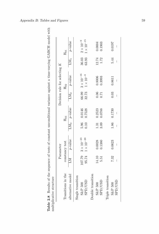
Appendix B: Tables and Figures 59
Tab
le2.
8R
esul
tsof
the
sequ
ence
ofte
sts
ofco
nsta
ntun
cond
itio
nal
vari
ance
agai
nst
ati
me-
vary
ing
GA
RC
Hm
odel
wit
hm
ulti
plic
ativ
est
ruct
ure
Par
amet
erD
ecis
ion
rule
for
sele
ctin
gK
Tra
nsit
ions
inth
eco
nsta
ncy
test
H03
H02
H01
alte
rnat
ive
mod
elL
Mp-
valu
eL
M3
p-va
lue
LM
2p-
valu
eL
M1
p-va
lue
Sing
letr
ansi
tion
S&P
500
107.
793×
10−
23
5.96
0.01
4666.9
93×
10−
16
36.0
32×
10−
9
SPD
/USD
95.7
41×
10−
20
0.10
0.75
2832.7
31×
10−
863.9
31×
10−
15
Dou
ble
tran
siti
onS&
P50
014.1
00.
0028
1.31
0.25
230.
060.
8006
12.7
40.
0004
SPD
/USD
5.51
0.13
803.
090.
0788
0.71
0.39
931.
720.
1903
Tri
ple
tran
siti
onS&
P50
07.
320.
0623
1.86
0.17
300.
030.
8611
5.44
0.01
97SP
D/U
SD−
−−
−−
−−
−

60 Chapter 2T
able
2.9
Mis
spec
ifica
tion
test
sfo
rth
eG
AR
CH
mod
els
inth
etw
oap
plic
atio
ns
No
AR
CH
-in-
GA
RC
HG
AR
CH
(1,1
)vs
GA
RC
H(1
,1)
vsN
oad
diti
onal
No
STG
AR
CH
r=
1r
=5
r=
10G
AR
CH
(1,2
)G
AR
CH
(2,1
)tr
ansi
tion
wit
hK
=1
S&P
500
LM
test
0.84
16.
167
7.22
30.
001
0.30
39.
993
20.0
88p-v
alue
0.35
90.
290
0.70
40.
971
0.58
20.
019
4×
10−
5
ε t/g
1/2
t S&
P500
LM
test
0.15
55.
115
6.82
40.
558
0.73
80.
677
45.3
87p-v
alue
0.69
40.
402
0.74
20.
455
0.39
00.
879
1×
10−
10
No
AR
CH
-in-
GA
RC
HG
AR
CH
(1,1
)vs
GA
RC
H(1
,1)
vsN
oad
diti
onal
No
STG
AR
CH
r=
1r
=5
r=
10G
AR
CH
(1,2
)G
AR
CH
(2,1
)tr
ansi
tion
wit
hK
=1
SPD
/USD
LM
test
0.34
312
.83
15.9
40.
666
2.77
214
.93
2.74
1p-v
alue
0.55
80.
025
0.10
10.
415
0.09
60.
002
0.25
4
ε t/g
1/2
t SP
D/
US
D
LM
test
0.01
46.
988
10.3
40.
064
2.60
72.
133
1.16
7p-v
alue
0.90
50.
222
0.41
10.
780
0.10
60.
545
0.55
8
Note
s:T
he
test
sare
those
again
stre
main
ing
AR
CH
inth
est
an
dard
ized
resi
du
als
,G
AR
CH
(1,2
)an
dG
AR
CH
(2,1
)m
od
els,
add
itio
nal
tran
siti
on
inth
efu
nct
iongt,
an
dS
TG
AR
CH
(1,1
)m
odel
of
ord
er1.

Appendix B: Tables and Figures 61
Tab
le2.
10M
issp
ecifi
cati
onte
sts
for
the
GJR
-GA
RC
Hm
odel
inth
est
ock
retu
rns
appl
icat
ion
No
AR
CH
-in-
GA
RC
HG
AR
CH
(1,1
)vs
GA
RC
H(1
,1)
vsN
oad
diti
onal
No
STG
AR
CH
r=
1r
=5
r=
10G
AR
CH
(1,2
)G
AR
CH
(2,1
)tr
ansi
tion
wit
hK
=1
S&P
500
LM
test
0.51
82.
094
3.06
021.8
748.
317
17.1
7616.8
04p-v
alue
0.47
20.
836
0.98
02×
10−
50.
004
7×
10−
40.
002
ε t/g
1/2
t S&
P500
LM
test
2.45
04.
963
7.82
18.
113
3.29
30.
184
11.2
35p-v
alue
0.11
80.
420
0.64
60.
017
0.07
00.
980
0.02
4
Note
s:T
he
test
sare
those
again
stre
main
ing
AR
CH
inth
est
an
dard
ized
resi
du
als
,G
AR
CH
(1,2
)an
dG
AR
CH
(2,1
)m
od
els,
ad
dit
ion
al
tran
siti
on
inth
efu
nct
iongt,
an
dS
TG
AR
CH
(1,1
)m
od
elof
ord
er1.

62 Chapter 2
0 250 500 750 1000 1250 1500 1750 2000 2250 25001.0
1.5
2.0
2.5
3.0
3.5
4.0
4.5
Figure 2.9 Graph of the final estimated function gt for the S&P 500 returns modelas a smooth function of the rescaled time variable t∗ as given in (2.54)-(2.56)

Appendix B: Tables and Figures 63
10 20 30 40 50 60 70 80 90 100
0.0
0.1
0.2
0.3
0.4
0.5
(a) S&P 500 returns
10 20 30 40 50 60 70 80 90 100
0.0
0.1
0.2
0.3
0.4
0.5
(b) 1st iteration
10 20 30 40 50 60 70 80 90 100
0.0
0.1
0.2
0.3
0.4
0.5
(c) 23rd iteration
Figure 2.10 Sample autocorrelations of absolute log returns of the S&P 500 andthe standardized variable |εt|/g1/2
tS&P500for the first and the final iterations with the
95% confidence bounds.

64 Chapter 2
0 250 500 750 1000 1250 1500 1750 2000 2250 25000.5
1.0
1.5
2.0
2.5
3.0
(a) S&P 500 returns
0 250 500 750 1000 1250 1500 1750 2000 2250 25000.5
1.0
1.5
2.0
2.5
3.0
(b) 1st iteration
0 250 500 750 1000 1250 1500 1750 2000 2250 25000.5
1.0
1.5
2.0
2.5
3.0
(c) 23rd iteration
Figure 2.11 Conditional standard deviation of the GJR-GARCH(1,1) model for theS&P 500 returns and the standardized variable εt/g
1/2tS&P500
for the first and the finaliterations.

Appendix B: Tables and Figures 65
−7 −6 −5 −4 −3 −2 −1 0 1 2 3 4 50.5
0.8
1.1
1.4
1.7
2.0
2.3
2.6
Figure 2.12 News impact curves of the GJR-GARCH(1,1) (solid line in boldface)and the TV-GJR-GARCH(1,1) models for several regimes. The time-varying newsimpact curves are plotted for the lower regime, i.e. G1(t∗) = G2(t∗) = 0 (dotted line),for an intermediate regime, i.e. G1(t∗) = 1 and G2(t∗) = 0 (dashed line) and for thehigher regime, i.e. G1(t∗) = G2(t∗) = 1 (solid line).

66 Chapter 2
0 300 600 900 1200 1500 1800 2100
0.2
0.3
0.4
0.5
0.6
0.7
0.8
0.9
1.0
Figure 2.13 Graph of the final estimated function gt for the SPD/USD returnsmodel as a smooth function of the rescaled time variable t∗ as given in (2.57)-(2.58).

Appendix B: Tables and Figures 67
10 20 30 40 50 60 70 80 90 100
0.0
0.1
0.2
0.3
0.4
0.5
(a) SPD/USD returns
10 20 30 40 50 60 70 80 90 100
0.0
0.1
0.2
0.3
0.4
0.5
(b) 1st iteration
10 20 30 40 50 60 70 80 90 100
0.0
0.1
0.2
0.3
0.4
0.5
(c) 41st iteration
Figure 2.14 Sample autocorrelations of absolute log returns of the SPD/USD andfor the standardized variable |εt|/g1/2
tSP D/USDfor the first and the final iterations with
the 95% confidence bounds.

68 Chapter 2
0 300 600 900 1200 1500 1800 2100
0.3
0.6
0.9
1.2
1.5
1.8
(a) SPD/USD returns
0 300 600 900 1200 1500 1800 2100
0.3
0.6
0.9
1.2
1.5
1.8
(b) 1st iteration
0 300 600 900 1200 1500 1800 2100
0.3
0.6
0.9
1.2
1.5
1.8
(c) 41st iteration
Figure 2.15 Conditional standard deviation of the GARCH(1,1) model for theSPD/USD returns and for the standardized variable εt/g
1/2tSP D/USD
for the first andthe final iterations.

Appendix B: Tables and Figures 69
−4 −3 −2 −1 0 1 2 30.2
0.5
0.8
1.1
1.4
1.7
2.0
2.3
2.6
Figure 2.16 News impact curves of the GARCH(1,1) (solid line in boldface) and theTV-GARCH(1,1) models for several regimes. The time-varying news impact curvesare plotted for the lower regime, i.e. G1(t∗) = 0 (dotted line), for an intermediateregime, i.e. G1(t∗) = 0.5 (dashed line) and for the higher regime, i.e. G1(t∗) = 1(solid line)


Bibliography
Anderson, H. M., K. Nam, and F. Vahid (1999): “Asymmetric Nonlinear SmoothTransition GARCH Models,” in Nonlinear Time Series Analysis of Economic andFinancial Data, ed. by P. Rothman, pp. 191–207. Kluwer Academic Publishers,Boston.
Baillie, R. T., T. Bollerslev, and H. O. Mikkelsen (1996): “FractionallyIntegrated Generalized Autoregressive Conditional Heteroskedasticity,” Journal ofEconometrics, 74, 3–30.
Baillie, R. T., and C. Morana (2007): “Modeling Long Memory and StructuralBreaks in Conditional Variances: An Adaptive FIGARCH Approach,” WorkingPaper No. 593, Queen Mary University of London, Department of Economics.
Berkes, I., E. Gombay, L. Horvath, and P. Kokoszka (2004): “SequentialChange-Point Detection in GARCH(p,q) Models,” Econometric Theory, 20, 1140–1167.
Berkes, I., L. Horvath, and P. Kokoszka (2003): “GARCH Processes: Structureand Estimation,” Bernoulli, 9, 201–207.
Bollerslev, T. (1986): “Generalized Autoregressive Conditional Heteroskedastic-ity,” Journal of Econometrics, 31, 307–327.
Bollerslev, T. (1990): “Modelling the Coherence in Short-Run Nominal ExchangeRates: A Multivariate Generalized ARCH Model,” The Review of Economic andStatistics, 72, 498–505.
Cai, J. (1994): “A Markov Model of Unconditional Variance in ARCH,” Journal ofBusiness & Economic Statistics, 12, 309–316.
Dahlhaus, R., and S. Subba Rao (2006): “Statistical Inference for Time-VaryingARCH Processes,” Annals of Statistics, 34, 1075–1114.
Davidson, R., and J. G. MacKinnon (1998): “Graphical Methods for Investigatingthe Size and Power of Hypothesis Tests,” The Manchester School, 66, 1–26.
Davies, R. B. (1977): “Hypothesis Testing When a Nuisance Parameter is PresentOnly under the Alternative,” Biometrika, 64, 247–254.
71

72 Bibliography
Diebold, F. X. (1986): “Comment on ”Modelling the Persistence of ConditionalVariance”, by R. Engle and T. Bollerslev,” Econometric Reviews, 5, 51–56.
Doornik, J. A. (2002): Object-Oriented Matrix Programming Using Ox. TimberlakeConsultants Press, see also www.nuff.ox.ac.uk/Users/Doornik, 3rd edn.
Eitrheim, Ø., and T. Terasvirta (1996): “Testing the Adequacy of Smooth Tran-sition Autoregressive Models,” Journal of Econometrics, 74, 59–75.
Engle, R. F. (1982): “Autoregressive Conditional Heteroskedasticity with Estimatesof the Variance of United Kingdom Inflation,” Econometrica, 50, 987–1007.
Engle, R. F., and J. Gonzalo Rangel (2008): “The Spline-GARCH Model forLow-Frequency Volatility and its Global Macroeconomic Causes,” Review of Fi-nancial Studies, 21, 1187–1222.
Fiorentini, G., G. Calzolari, and L. Panattoni (1996): “Analytic Derivativesand the Computation of GARCH Estimates,” Journal of Applied Econometrics,11, 399–417.
Gallant, R. (1984): “The Fourier Flexible Form,” American Journal of AgriculturalEconomics, 66, 204–208.
Geweke, J., and S. Porter-Hudak (1983): “The Estimation and Application ofLong-Memory Time-Series Models,” Journal of Time Series Analysis, 4, 221–238.
Gonzalez-Rivera, G. (1998): “Smooth Transition GARCH Models,” Studies inNonlinear Dynamics and Econometrics, 3, 61–78.
Granger, C. W. J. (1993): “Strategies for Modelling Nonlinear Time-Series Rela-tionships,” Economic Record, 69, 233–239.
Hagerud, G. E. (1997): “A New Non-Linear GARCH Model,” Ph.D. thesis, EFI,Stockholm School of Economics.
Hamilton, J. D., and R. Susmel (1994): “Autoregressive Conditional Het-eroskedasticity and Changes in Regime,” Journal of Econometrics, 64, 307–333.
Hansen, B. E. (1996): “Inference When a Nuisance Parameter is Not Identifiedunder the Null Hypothesis,” Econometrica, 64, 413–430.
Jensen, S. T., and A. Rahbek (2004): “Asymptotic Inference for NonstationaryGARCH,” Econometric Theory, 20, 1203–1226.
Kim, T.-H., and H. White (2004): “On More Robust Estimation of Skewness andKurtosis,” Finance Research Letters, 1, 56–73.
Lamoureux, C. G., and W. D. Lastrapes (1990): “Persistence in Variance, Struc-tural Change, and the GARCH Model,” Journal of Business & Economic Statistics,8, 225–234.

Bibliography 73
Li, W. K., and T. K. Mak (1994): “On the Squared Residual Autocorrelationsin Non-Linear Time Series With Conditional Heteroskedasticity,” Journal of TimeSeries Analysis, 15, 627–636.
Lin, C.-F. J., and T. Terasvirta (1994): “Testing the Constancy of RegressionParameters Against Continuous Structural Change,” Journal of Econometrics, 62,211–228.
Ling, S., and W. Li (1997): “Diagnostic Checking of Nonlinear Multivariate TimeSeries with Multivariate ARCH Errors,” Journal of Time Series Analysis, 18, 447–464.
Ling, S., and M. McAleer (2003): “Asymptotic Theory for a New Vector ARMA-GARCH Model,” Econometric Theory, 19, 280–310.
Lundbergh, S., and T. Terasvirta (2002): “Evaluating GARCH Models,” Jour-nal of Econometrics, 110, 417–435.
Luukkonen, R., P. Saikkonen, and T. Terasvirta (1988): “Testing LinearityAgainst Smooth Transition Autoregressive Models,” Biometrika, 75, 491–499.
Meitz, M., and P. Saikkonen (in press): “Ergodicity, Mixing, and Existence ofMoments of a Class of Markov Models with Applications to GARCH and ACDModels,” Econometric Theory.
Mikosch, T., and C. Starica (2004): “Nonstationarities in Financial Time Series,the Long-Range Dependence, and the IGARCH Effects,” The Review of Economicsand Statistics, 86, 378–390.
Terasvirta, T. (1994): “Specification, Estimation, and Evaluation of Smooth Tran-sition Autoregressive Models,” Journal of the American Statistical Association, 89,208–218.
(1998): “Modeling Economic Relationships with Smooth Transition Regres-sions,” in Handbook of Applied Economic Statistics, ed. by A. Ullah, and D. Giles,pp. 507–552. New York: Dekker.
Terasvirta, T., and Z. Zhao (2007): “Stylized Facts of Return Series, RobustEstimates, and Three Popular Models of Volatility,” SSE/EFI Working Paper Seriesin Economics and Finance No. 662.
Wooldridge, J. M. (1990): “A Unified Approach to Robust, Regression-BasedSpecification Tests,” Econometric Theory, 6, 17–43.
(1991): “On the Application of Robust, Regression-Based Diagnostics toModels of Conditional Means and Conditional Variances,” Journal of Econometrics,47, 5–46.


Chapter 3
Modelling Changes in theUnconditional Variance ofLong Stock Return Series
75


77
Modelling Changes in the Unconditional Variance of
Long Stock Return Series1
Abstract
In this paper we develop a testing and modelling procedure for describing the long-term movements over very long return series. For the purpose, we assume that volatil-ity is multiplicatively decomposed into a conditional and an unconditional componentas in Amado and Terasvirta (2008). The latter component is modelled by incorpo-rating smooth changes so that the unconditional variance is allowed to evolve slowlyover time. Statistical inference is used for specifying the parameterization of thetime-varying component by applying a sequence of Lagrange multiplier tests. Themodel building procedure is illustrated with an application to the daily returns ofthe DJIA index covering a period of eighty three years of financial market history.Two major conclusions are as follows. First, the LM tests strongly reject the as-sumption of constancy of the unconditional variance. Second, the results show thatthe long-memory property in volatility may be explained by ignored changes in theunconditional variance of the long series.
1This paper is a joint work with Timo Terasvirta.Acknowledgements: The first author would like to acknowledge financial support from the
Louis Fraenckels Stipendiefond. Part of this research was done while the first author was visitingCREATES, University of Aarhus, whose kind hospitality is gratefully acknowledged. The Centerfor Research in Econometric Analysis of Time Series, CREATES, is funded by the Danish NationalResearch Foundation. The responsibility for any errors and shortcomings in this paper remains ours.

78 Chapter 3
3.1 Introduction
The observation that deterministic shifts in long return series can generate long-memory behaviour has received much attention in recent years. Most of the work inthis topic is related with the study of the behaviour of standard statistical tools andmodel misspecification under nonstationarity. Early studies include Diebold (1986)and Lamoureux and Lastrapes (1990) who suggested that occasional level shifts inthe intercept of the first-order GARCH model can bias the estimation towards anintegrated GARCH model. More recently, Mikosch and Starica (2004) argued thatthe so-called ‘integrated GARCH effect’ is caused by the nonstationary behaviour ofvery long return series. They show how the long-range dependence in volatility andthe IGARCH effect may be explained by neglected deterministic changes in the un-conditional variance of the stochastic process. Moreover, Granger and Hyung (2004)claimed that occasional breaks in a long time series of absolute stock returns can alsoexplain the observed slow decay of the autocorrelation functions of absolute returnsin long return series.
It is well documented that shocks to the conditional variance of the standardGARCH model of Bollerslev (1986) decay at an exponential rate. This has motivatedthe development of more flexible models to describe the observed dependence structurein financial market volatility. One of these models is the Fractionally IntegratedGARCH model of Baillie, Bollerslev, and Mikkelsen (1996) which belongs to theclass of long-memory models. In these processes, shocks to the conditional variancedecay at a slow hyperbolic rate which is more strongly supported by financial datathan the GARCH model. A generalization of the FIGARCH model was recentlyproposed by Baillie and Morana (2007) in which they allow the intercept to changedeterministically according to the flexible functional form of Gallant (1984).
The question of explicitly modelling nonstationarity in stock market volatilityhas, however, received somewhat less attention. There have been some attempts toincorporate nonstationarity directly into the model. Starica and Granger (2005) intro-duced a nonstationary approach in which the returns are modelled as nonstationarysequence of independent random variables with time-varying unconditional variancebut their model does not allow for volatility clustering. More recently, Engle andGonzalo Rangel (2008) proposed modelling the volatility process by a multiplicativedecomposition into a nonstationary and a stationary component. The nonstationarycomponent (or the unconditional variance) is described by an exponential spline, andthe stationary component (or the short-run dynamics of volatility) follows a first-orderGARCH process.
This paper addresses the issue of modelling deterministic changes in the uncon-ditional variance of long return series. It is assumed that volatility is modelled bydecomposing the variance into a conditional and an unconditional component as inAmado and Terasvirta (2008). The conditional variance follows a GARCH process,and describes the short-run dynamics of volatility. The nonstationary componentof volatility describes the long-volatility dynamics, and it is represented by a linearcombination of logistic transition functions. Statistical inference is used for specifyingthe parametric structure of the time-varying component by applying a sequence of

Modelling Changes in the Unconditional Variance 79
Lagrange multiplier tests. Our modelling strategy is applied to describe the long-runproperties of the long daily Dow Jones Industrial Average (DJIA) return series from1920 to 2003. One may expect that the longer the observation period, the more likelythe occurrence of structural changes or shifts in the second unconditional momentof returns. The test results strongly support the time-variation of the unconditionalvariance in the period under study. The estimation results indicate that the strongestdeterministic changes in the unconditional variance are associated with the largesteconomic recessions. This in turn suggests that the unconditional variance behaviourmay be related to the evolution of the deterministic conditions in the economy. Ourfindings also suggest that the observed long-memory property in volatility may wellbe due to deterministic changes in the unconditional variance of the return series.
The paper is organized as follows. The TV-GARCH model and the modellingstrategy are presented in Section 3.2. Details regarding the estimation of the modelare discussed in Section 3.3. Section 3.4 contains the application. In Section 3.5 weshow by a small Monte Carlo simulation how ignored deterministic changes in theunconditional variance affect the estimation of a misspecified model. Finally, Section3.6 concludes.
3.2 A model for the long-term volatility component
3.2.1 The time-varying GARCH framework
In this paper the tool for modelling an asset return series over a long period isa GARCH-type model in which the unconditional variance is assumed to evolvesmoothly over time. To motivate the introduction of our model we shall begin byfocusing on the long-run properties of the GJR-GARCH(p, q) model of Glosten, Ja-gannathan, and Runkle (1993). Let Ft−1 be the information set containing the his-torical information of the series of interest available at time t− 1 and write the assetreturns {yt} as
yt = E(yt|Ft−1) + εt (3.1)
εt = ζth1/2t (3.2)
where {ζt} is a sequence of independent standard normal variables. Under this as-sumption the conditional distribution of the innovation sequence {εt} is εt|Ft−1 ∼N(0, ht). For simplicity, the conditional mean of the asset returns is set equal to zero,i.e. E(yt|Ft−1) = 0. The component ht describes the dynamics of the conditionalvariance of the asset returns. To allow positive and negative shocks to have an asym-metric effect on the stock market volatility we choose the GJR-GARCH(p, q) modelfor ht. It has the form
ht = ω +q∑i=1
αiε2t−i +
q∑i=1
κiε2t−iIt−i(εt−i < 0) +
p∑j=1
βjht−j . (3.3)
where the set of conditions for positivity and stationarity are imposed and It−i(εt−i <0) is an indicator function that equals 1 when εt−i < 0, i = 1, . . . , q, and 0 otherwise.
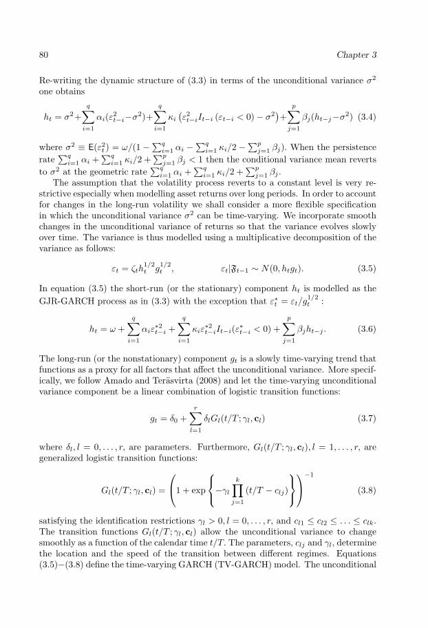
80 Chapter 3
Re-writing the dynamic structure of (3.3) in terms of the unconditional variance σ2
one obtains
ht = σ2+q∑i=1
αi(ε2t−i−σ2)+q∑i=1
κi(ε2t−iIt−i (εt−i < 0)− σ2
)+
p∑j=1
βj(ht−j−σ2) (3.4)
where σ2 ≡ E(ε2t ) = ω/(1 −∑qi=1 αi −
∑qi=1 κi/2 −
∑pj=1 βj). When the persistence
rate∑qi=1 αi +
∑qi=1 κi/2 +
∑pj=1 βj < 1 then the conditional variance mean reverts
to σ2 at the geometric rate∑qi=1 αi +
∑qi=1 κi/2 +
∑pj=1 βj .
The assumption that the volatility process reverts to a constant level is very re-strictive especially when modelling asset returns over long periods. In order to accountfor changes in the long-run volatility we shall consider a more flexible specificationin which the unconditional variance σ2 can be time-varying. We incorporate smoothchanges in the unconditional variance of returns so that the variance evolves slowlyover time. The variance is thus modelled using a multiplicative decomposition of thevariance as follows:
εt = ζth1/2t g
1/2t , εt|Ft−1 ∼ N(0, htgt). (3.5)
In equation (3.5) the short-run (or the stationary) component ht is modelled as theGJR-GARCH process as in (3.3) with the exception that ε∗t = εt/g
1/2t :
ht = ω +q∑i=1
αiε∗2t−i +
q∑i=1
κiε∗2t−iIt−i(ε
∗t−i < 0) +
p∑j=1
βjht−j . (3.6)
The long-run (or the nonstationary) component gt is a slowly time-varying trend thatfunctions as a proxy for all factors that affect the unconditional variance. More specif-ically, we follow Amado and Terasvirta (2008) and let the time-varying unconditionalvariance component be a linear combination of logistic transition functions:
gt = δ0 +r∑l=1
δlGl(t/T ; γl, cl) (3.7)
where δl, l = 0, . . . , r, are parameters. Furthermore, Gl(t/T ; γl, cl), l = 1, . . . , r, aregeneralized logistic transition functions:
Gl(t/T ; γl, cl) =
1 + exp
−γlk∏j=1
(t/T − clj)
−1
(3.8)
satisfying the identification restrictions γl > 0, l = 0, . . . , r, and cl1 ≤ cl2 ≤ . . . ≤ clk.The transition functions Gl(t/T ; γl, cl) allow the unconditional variance to changesmoothly as a function of the calendar time t/T. The parameters, clj and γl, determinethe location and the speed of the transition between different regimes. Equations(3.5)−(3.8) define the time-varying GARCH (TV-GARCH) model. The unconditional

Modelling Changes in the Unconditional Variance 81
variance in this model is time-varying and equals Et(ε2t ) =E(ζ2t htgt) = gtEht. This
approach of introducing nonstationarity in the long run volatility component has beendiscussed in detail by Amado and Terasvirta (2008).
Some special cases of the TV-GARCH model are of interest. Under δ1 = . . . =δr = 0, the unconditional variance Et(ε2t ) becomes constant. When r = 1 and k = 1, gtincreases (decreases) monotonically over time from δ0 to δ0 + δ1 when δ1 > 0(δ1 < 0),with the location centred at t = c1T. The slope parameter γ1 in (3.8) controls thedegree of smoothness of the transition: the larger γ1, the faster the transition isbetween the extreme regimes. When γ1 → ∞, gt collapses into a step function. Forsmall values of γ1, the transition between regimes is approximately linear aroundc1. When δl 6= 0, for values r > 1 and k > 1, (3.7)−(3.8) form a very flexibleparameterization capable of describing nonmonotonic deterministic changes in theunconditional variance.
3.2.2 Model specification
Since the nonlinear model in (3.5)−(3.8) is our most general parameterization, asystematic modelling strategy is required when a TV-GARCH model is fitted to thedata. The strategy for building TV-GARCH models is based on statistical inferenceand it consists of the specification, estimation and evaluation of the model. At thespecification stage, one first specifies the structure of gt and, once that has been done,models the dynamics of the short-run component ht. In practice, the parametricstructure of the unconditional variance component has to be determined from thedata, which involves two sets of decision problems. First, the number of transitions rin (3.7) has to be determined. Second, when r ≥ 1, the integer k for each transitionfunction has to be selected. This specification procedure is sequential and based onstatistical inference. We shall apply the procedure of Amado and Terasvirta (2008)for selecting r and k.
An important feature of the modelling strategy in this paper is that, since weare modelling very long return series, we shall divide the observation period into anumber of subperiods. To introduce notation, let r be the total number of tran-sitions in the whole period and ri, i = 1, . . . , N, be the number of transitions inthe subperiod i, so r =
∑Ni=1 ri. Define hit as the conditional variance and git =
1 +∑ri
l=1 δilGil(t/T ; γl, cl), i = 1, . . . , N, for each subperiod.The sequence of LM tests for specifying a TV-GARCH model is as follows:
1. Split the original time series into N non-overlapping subsamples. To facilitatespecification the splits should preferably be located in tranquil periods.
2. For each i = 1, . . . , N, specify git under the assumption that the conditionalvariance is constant, i.e. hit ≡ ωi > 0. This is done as follows. First, test thehypothesis of constant unconditional variance H01 : γi1 = 0 against H11 : γi1 > 0in
git = ω−1i {1 + δi1Gi1 (t/T ; γi1, ci1)} = ω−1
i + δ∗i1Gi1(t/T ; γi1, ci1) (3.9)

82 Chapter 3
where δ∗i1 = ω−1i δi1, at the significance level α(1). Under the null hypothesis, the
function contains unidentified nuisance parameters δi1 and ci1. To circumventthis identification problem we follow Luukkonen, Saikkonen, and Terasvirta(1988) and approximate Gi1(t/T ; γi1, ci1) by its third-order Taylor expansionaround γi1 = 0. After reparameterizing, we obtain
git = ω∗i +3∑j=1
φij(t/T )j +R3(t/T ; γi1, ci1) (3.10)
where φij = γi1δ∗ij , i = 1, . . . , N, and R3(t/T ; γi1, ci1) is the remainder. Further-
more, R3(t/T ; γi1, ci1) ≡ 0 under H01, so the remainder of the Taylor expansiondoes not affect the asymptotic distribution theory. The null hypothesis of con-stant unconditional variance becomes H
′
01 : φi1 = φi2 = φi3 = 0. Under H′
01, thestandard LM statistic has an asymptotic χ2−distribution with three degrees offreedom. See Amado and Terasvirta (2008) for details on how to compute thetest statistic.
3. If H′
01 is rejected, for each subperiod select the order k ≤ 3 in the exponentof Gi1(t/T ; γi1, ci1) using a short sequence of tests within (3.10); for detailssee Amado and Terasvirta (2008). Next, estimate git with a single transitionfunction and test H02 : git = ω−1
i +δ∗i1Gi1(t/T ; γi1, ci1) against H12 : git = ω−1i +∑2
l=1 δ∗ilGil(t/T ; γil, cil) at the significance level α(2) = τα(1), where τ ∈ (0, 1).
The significance level is reduced at each stage by a factor τ in order to favourparsimony. In our application we set τ = 0.5. Test the hypothesis of no secondtransition H02 : γi2 = 0 in
git = ω−1i + δ∗i1Gi1(t/T ; γi1, ci1) + δ∗i2Gi2(t/T ; γi2, ci2) (3.11)
Again, model (3.11) is not identified under the null hypothesis. To circumventthe problem we proceed as before and express the logistic functionGi2(t/T ; γi2, ci2)by a third-order Taylor approximation around γi2 = 0. After rearranging termswe have
git = ω∗i + δ∗i1Gi1(t/T ; γi1, ci1) +3∑j=1
ϕij(t/T )j +R∗3(t/T ; γi2, ci2) (3.12)
where ϕij = γi2δ∗ij , i = 1, . . . , N, and R∗3(t/T ; γi2, ci2) is the remainder. The
new null hypothesis based on this approximation is H′
02 : ϕi1 = ϕi2 = ϕi3 = 0.Again, this hypothesis can be tested using a LM test. If the null hypothesis isrejected, specify k for the second transition and estimate git with two transitionfunctions.
4. More generally, when git has been estimated with ri−1 transition functions onetests for another transition in git using the significance level α(ri) = τα(ri−1).Testing continues until the first non-rejection of the null hypothesis.

Modelling Changes in the Unconditional Variance 83
In summary, we begin the model specification problem by first modelling the un-conditional variance assuming that the conditional variances remain constant. Afterspecifying and estimating gt, the hypothesis of no conditional heteroskedasticity istested in {ε∗t }. If the null hypothesis of no ARCH is rejected, the conditional variancecomponent ht is modelled as in (3.6) with p = q = 1. At the evaluation stage theadequacy of the estimated model is tested by means of LM-type misspecification tests(see Amado and Terasvirta (2008) for further details).
3.3 Estimation of parameters
After the number of transitions and their type in (3.7) have been determined, theparameters of the TV-GARCH model are estimated by quasi-maximum likelihood(QML). For this purpose, let θ = (θ′1,θ
′2)′ be the parameter vector of the model.
Let ht ≡ ht(θ1,θ2) and gt ≡ gt(θ2) where θ1 = (ω, α1, . . . , αq, κ1, . . . , κq, β1, . . . , βp)′
and θ2 = (δ′, γ1, . . . , γr, c′1, . . . , c′r)′ with δ = (δ0, δ1, . . . , δr)′. The model defined in
(3.5)−(3.8) can be now rewritten as follows:
εt = ζt {ht (θ1,θ2) gt (θ2)}1/2 . (3.13)
Assuming that {ζt} is a sequence of independent standard normal variables, the log-likelihood function for observation t equals
`t(θ) = −(1/2) ln 2π− (1/2){lnht(θ1,θ2)+ln gt(θ2)}− (1/2)ε2t
ht(θ1,θ2)gt(θ2)(3.14)
The unconditional and the conditional variance components are estimated separatelyusing maximization by parts. The iterative algorithm proceeds as follows:
Step 1: Maximize
LUT (θ2) =T∑t=1
`Ut (θ2) = −(1/2)T∑t=1
{ln gt(θ2) + ε2t/gt(θ2)}
with respect to θ2, assuming εt = εt, that is, setting ht(θ1,θ2) ≡ 1. Let the
estimator of θ2 be θ(1)
2 . Making use of θ(1)
2 , maximize
LVT (θ1, θ(1)
2 ) =T∑t=1
`Vt (θ1, θ(1)
2 ) = −(1/2)T∑t=1
{lnht(θ1, θ
(1)
2 ) + ε∗2t /ht(θ1, θ(1)
2 )}
with respect to θ1, where ε∗t = εt/{gt(θ(1)
2 )}1/2. Denote the estimator as θ(1)
2 .
Step 2: Maximize
LUT (θ2) =T∑t=1
`Ut (θ2) = −(1/2)T∑t=1
{ln gt(θ2) + ε2t/gt(θ2)}
84 Chapter 3
with respect to θ2, where εt = εt/{ht(θ(1)
1 , θ(1)
2 )}1/2. Call this estimator θ(2)
2
and maximize
LVT (θ1, θ(2)
2 ) =T∑t=1
`Vt (θ1, θ(2)
2 ) = −(1/2)T∑t=1
{lnht(θ1, θ
(2)
2 ) + ε∗2t /ht(θ1, θ(2)
2 )}
with respect to θ1, where ε∗t = εt/{gt(θ(2)
2 )}1/2. This yields θ(2)
1 .
Iterate until convergence.
In the nth iteration, maximization is carried out in the usual way by solving thescore equations:
∂
∂θ2LUT (θ2) = (1/2)
T∑t=1
(ε2t
gt(θ2)− 1)
1gt(θ2)
∂gt(θ2)∂θ2
= 0
for θ2 with εt = εt/{ht(θ(n−1)
1 , θ(n−1)
2 )}1/2, and
∂
∂θ1LVT (θ1) = (1/2)
T∑t=1
(ε∗2t
ht(θ1, θ(n)
2 )− 1
)1
ht(θ1, θ(n)
2 )
∂ht(θ1, θ(n)
2 )∂θ1
= 0
for θ1, where ε∗t = εt/{gt(θ(n)
2 )}1/2. Letting Glt ≡ Gl(t/T ; γl, cl), l = 1, . . . , r, we have
∂gt(θ2)∂θ2
= (1, G1t, G(γ)1t , G
(c)1t , . . . , Grt, G
(γ)rt , G
(c)rt )′
where, for k = 1 in (3.8),
G(γ)lt =
∂Glt∂γl
= δlGlt(1−Glt)(t/T − cl)
G(c)lt =
∂Glt∂cl
= −γlδlGlt(1−Glt)
and for k > 1
G(γ)lt =
∂Glt∂γl
= δlGlt(1−Glt)∏k
j=1(t/T − clj)
G(c)ilt =
∂Gilt∂cl
= −γlδlGlt(1−Glt)∏k
j=1,j 6=l(t/T − clj)
where clj denotes the jth element in the parameter vector cl, l = 1, . . . , r, and
∂ht(θ1, θ(n)
2 )∂θ1
= (1, ε∗2t−1, . . . , ε∗2t−q, ε
∗2t−1It−1(ε∗t−1 < 0), . . . , ε∗2t−qIt−q(ε
∗t−q < 0),
ht−1(θ1, θ(n)
2 ), . . . , ht−p(θ1, θ(n)
2 ))′ +p∑j=1
βj∂ht−j(θ1, θ
(n)
2 ))∂θ1

Modelling Changes in the Unconditional Variance 85
This algorithm is computationallly attractive for situations in which direct maxi-mization of the log-likelihood function is difficult. Under certain regularity conditions,the resulting estimator coincides with the ML estimator and becomes fully efficientupon convergence; see Song, Fan, and Kalbfleisch (2005) for details. Throughout thispaper, we assume that certain regularity conditions are satisfied to ensure consistencyand asymptotic normality of the QML estimator. The asymptotic properties of theestimators of the TV-GARCH model are not yet known. Extending the results to thenonstationary TV-GARCH model is not straightforward and is beyond the scope ofthis paper.
In this work, the long time series requires some modifications to the estimationalgorithm. Because the whole series is divided into non-overlapping subperiods, thedifferent data segments can have different “baseline” volatility levels. For this reason,the algorithm iterates from an initial value which is estimated by “chain rule” toaccommodate differences in the volatility levels. This proceeds as follows. First, forthe first subperiod, estimate the parameters of g1t = δ0 +
∑r1l=1 δ1lG1l(t/T ; γ1l, c1l)
where r1 is the number of transitions for this period. The estimate g1t serves as the“intercept” in the nonstationary component of the next subperiod. Conditioning onthis value, carry out the estimation of the parameters for the next subperiod. Moregenerally, for the ith subperiod, estimate git = δ
(i−1)0 +
∑ri
l=1 δilGil(t/T ; γil, cil) byconditioning on δ
(i−1)0 , where δ
(i−1)0 = δ0 +
∑ri−1l=1 δlGl(t/T ; γl, cl) and ri−1 is the
number of transitions in the (i − 1)th subperiod. The estimates γl and cl are thenused as fixed values in the next iterations. This means that the estimation algorithmis carried out without iterating γl and cl, and therefore the parameters δl, l = 0, . . . , r,are estimated conditionally on those estimates.
Another aspect that deserves attention in the estimation of the model is the selec-tion of starting-values of the time-varying parameters. Since the log-likelihood maycontain several local maxima, it is advisable to initiate the estimation from differentsets of starting-values before settling for the final parameter estimates. In addition,to improve the accuracy of the estimates of the standard errors, we follow Fiorentini,Calzolari, and Panattoni (1996) and use analytic first derivatives both in the esti-mation of the TV-GARCH models and in the computation of the test statistics. Allcomputations in this paper have been carried out using Ox programming language,version 3.40 (see Doornik (2002)).
3.4 Application to the Dow Jones Industrial Aver-age index
3.4.1 Data description
In this section we illustrate the use of the modelling building procedure of the TV-GARCH model to the daily returns of the Dow Jones Industrial Average (DJIA)index. The entire sample covers the period between January 2, 1920 and December31, 2003, yielding 21121 observations. The daily returns are defined as the log dif-ferences of the closing prices of the index between two consecutive days. The closing

86 Chapter 3
Table 3.1 Summary statistics of the daily DJIA return series: full sample
Series Min Max Mean S.D. Skew Ex.Kr. Rob.Sk. Rob.Kr.
εt -25.63 14.27 0.022 1.136 -0.659 25.28 -0.006 0.227
εt/g1/2t -17.71 6.680 0.018 0.660 -1.185 29.73 -0.006 0.145
Notes: The table contains summary statistics for the DJIA return series. The sample periodstarts in January 2, 1920 and ends in December 31, 2003 (21121 observations).
prices of the DJIA index have been obtained from the Wharton Research Data Ser-vices (WRDS) provided by the Wharton School of the University of Pennsylvania.Descriptive statistics of the return series can be found in Table 3.1. The coefficientsof skewness and kurtosis seem to indicate that the stock returns εt have a left skewedand a significantly fat-tailed distribution. To check this conclusion, we also providethe robust measures of skewness and kurtosis as recommended by Kim and White(2004) in order to account for outliers. The robust measure for skewness is practicallyzero whereas the robust kurtosis measure suggests that there is indeed some excesskurtosis in the series. Figure 3.1 graphs the daily returns for the DJIA index for theobservation period. The period covers the Great Depression of 1929 and the early1930’s, the Second World War, the 1973 oil crisis, the stock market crash of October1987 and the recent dot-com bubble. Because of the long observation period it isunlikely that the series is stationary.
We divide the 83 years long series into six non-overlapping subperiods each com-prising at least of 2500 observations. In most cases we report the findings for eachof the six periods and the full sample. Summary statistics of the subperiods can befound in Table 3.9.
3.4.2 Estimation results
The focus of the empirical analysis lies in the specification of the unconditional vari-ance using the modelling strategy described in Section 3.2.2. We begin by determiningthe number of transitions for each subperiod separately. This is done using the se-quence of specification tests. The initial significance level of the sequence of tests isα(1) = 0.01. At each stage of the sequence we halve the significance level of the test,i.e. τ = 0.5. The tests results are presented in the second column of Table 3.2.
We first test the hypothesis of constant unconditional variance against a smoothlytime-varying unconditional variance with one transition function. The null hypothesisis rejected for all subperiods with the exception of the subperiod 5 covering the Oc-tober 1987 crash. The stock market volatility returned to normal levels very quicklyafter the crash, which suggests that the unconditional variance remained stable duringthat period. These findings are consistent with the hypothesis of Engle and Lee (1999)that the 1987 crash is more transient than other big shocks. The null hypothesis ofconstant unconditional variance is, however, rejected very strongly for the subperiods1, 2, 4 and 6. The first period contains the Great Depression, the second includes the

Modelling Changes in the Unconditional Variance 87
500 1000 1500 2000 2500 3000 3500 4000−15−10−5
05
1015
4500 5000 5500 6000 6500 7000 7500 8000−10
−5
0
5
10
8500 9000 9500 10000 10500 11000 11500 12000 12500
−5
−2
1
4
7
12700 13200 13700 14200 14700 15200 15700 16200 16700
−5
−2
1
4
7
17000 17500 18000 18500 19000 19500 20000 20500 21000−25
−15
−5
5
15
Figure 3.1 The DJIA daily returns from January 2, 1920 until December 31, 2003.The vertical lines represent the split dates.
Second World War, the fourth one the OPEC oil crisis and the most recent one theIT bubble. The results indicate that the strongest deterministic changes in the un-conditional variance are associated with the largest economic recessions in the periodunder study.
The sequence of nested tests based on (3.10) to select k in (3.8) are given in thelast three columns of Table 3.2 (see Amado and Terasvirta (2008) for details). Thestrongest rejection is when k = 1 for all four periods. Note that, for the subperiod 1,the tests H01 and H02 cannot discriminate between k = 1 and k = 2 as the p-valuesare very close to each other. We choose k = 2 to minimize the number of transitions tobe specified. Misspecification tests to check the validity of this choice can be carriedout at the model evaluation stage.
We proceed to first estimate a TV-GARCH model with a single transition andtest against a double transition model at α(2) = 0.005. We reject the hypothesis inthree out of the five cases and select k = 1. Fitting the model with two transitionfunctions for the three subsamples and testing against another transition leads to arejection only for the fourth period. The p-value, however, is 0.0021 which is veryclose to α(3) = 0.0025. Thus, we tentatively accept the model with two transitions asthe final parameterization for the first, second and fourth subperiods.
The above results imply that eight transition functions in total are needed todescribe the unconditional variance for the whole series. Estimation results for the

88 Chapter 3
Table 3.2 p-values of sequences of Lagrange multiplier tests for the six subperiods
Subperiods H0 H03 H02 H01
Subsample 1 (02/01/1920 − 31/12/1931)Single transition 5× 10−44 7× 10⁻⁴ 3× 10⁻²² 3× 10⁻²⁴
Double transition 2× 10⁻⁸ 0.4773 0.0111 2× 10⁻⁸
Triple transition 0.2632 0.0574 0.7178 0.6213
Subsample 2 (04/01/1932 − 31/12/1943)Single transition 5× 10−77 3× 10⁻¹⁹ 3× 10⁻²⁰ 2× 10−46
Double transition 2× 10⁻⁶ 0.0017 0.0242 1× 10⁻⁴
Triple transition 0.2818 0.1547 0.3484 0.3388
Subsample 3 (04/01/1944 − 29/12/1961)Single transition 0.0079 0.0712 0.9654 0.0034Double transition 0.0792 0.2789 0.2364 0.0402Triple transition − − − −
Subsample 4 (01/01/1962 − 16/11/1982)Single transition 1× 10⁻¹⁷ 2× 10⁻⁴ 0.3328 3× 10⁻¹⁶
Double transition 4× 10⁻⁵ 9× 10⁻⁴ 0.8199 6× 10⁻⁴
Triple transition 0.0021 0.1889 0.0006 0.2988
Subsample 5 (17/11/1982 − 31/12/1993)Single transition 0.1018 0.8983 0.0173 0.4688Double transition − − − −
Subsample 6 (03/01/1994 − 31/12/2003)Single transition 3× 10⁻¹⁸ 0.0012 0.0017 8× 10⁻¹⁶
Double transition 0.0315 0.0361 0.0694 0.2817Triple transition − − − −
Notes: The entries are the p-values of the LM-type tests of constant unconditional variance against atime-varying GARCH model for each subperiod of the DJIA stock index returns. The test sequencestarts at the significance level α = 0.01 and setting τ = 0.5. The order k in (3.8) is chosen from thesequence of nested tests based on (3.10). If H 0i is rejected most strongly, measured by the p-value,of the three hypotheses, one selects k = i. See Amado and Terasvirta (2008) for further details.

Modelling Changes in the Unconditional Variance 89
Table 3.3 Estimation results for the DJIA returns: full samplePanel (a): parameter estimates of the TV-GJR-GARCH(1,1) model
ht = 0.0285(0.0052)
+ 0.0236(0.00386)
ε∗2t−1 + 0.9011(0.0136)
ht−1 + 0.0913(0.0166)
It−1(ε∗t−1 < 0)ε∗2t−1
Log-Lik = −19112.1 α1 + β1 + κ1/2 = 0.9704
gt = 0.82506(0.0276)
+ 1.1680(0.1382)
(1 + exp{−52.81(−)
(t/T − 0.0119(−)
)(t/T − 0.1047(−)
)})−1
+6.3472(0.3886)
(1 + exp{−100(−)
(t/T − 0.1154(−)
)})−1
− 6.4953(0.37118)
(1 + exp{−96.65(−)
(t/T − 0.1643(−)
)})−1
−1.2475(0.0657)
(1 + exp{−70.03(−)
(t/T − 0.2454(−)
)})−1
−0.1522(0.0188)
(1 + exp{−100(−)
(t/T − 0.3697(−)
)})−1
+1.7541(0.1486)
(1 + exp{−67.17(−)
(t/T − 0.6355(−)
)})−1
−1.2656(0.1495)
(1 + exp{−100(−)
(t/T − 0.6544(−)
)})−1
+0.6952(0.0599)
(1 + exp{−100(−)
(t/T − 0.9216(−)
)})−1
Panel (b): parameter estimates of the GJR-GARCH(1,1) model
ht = 0.0116(0.0021)
+ 0.0304(0.0039)
ε∗2t−1 + 0.9208(0.0085)
ht−1 + 0.0784(0.0123)
It−1(ε∗t−1 < 0)ε∗2t−1
Log-Lik = −27468.5 α1 + β1 + κ1/2 = 0.9903
TV-GARCH model are reported in Table 3.3, Panel (a). The estimation results foreach of the subperiods can be found in Table 3.10 in Appendix B.
The estimation is carried out with the sequential quadratic programming opti-misation algorithm using analytical derivatives. The numbers in parenthesis belowthe parameter estimates are the asymptotic standard error estimates and calculatedusing numerical second derivatives. The standard errors of γi and ci, i = 1, . . . , 8,are not available because the parameters δj , j = 0, . . . , 8, are estimated conditionallyon those parameters. In some subperiods we observe that the transition between theextreme regimes of volatility is quite rapid. For these cases, the maximum value of γjis constrained to 100 to avoid convergence problems. This approximation is adequatebecause the shape of the transition function does not change much beyond values ofγj larger or equal than 100.
For an idea how the unconditional variance changes over time, the estimatedcomponent g1/2
t is plotted in Figure 3.2 (upper panel). The estimated gt functionsfor each subperiod are also shown in Figure 3.8 (Appendix A). It is seen that the

90 Chapter 3
0 2500 5000 7500 10000 12500 15000 17500 20000
1
3
5
7
9
0 2500 5000 7500 10000 12500 15000 17500 20000
1
3
5
7
9
Figure 3.2 First panel, shows the estimated function g1/2t (black curve) and
the conditional standard deviation from the GJR-GARCH(1,1) model (grey curve).Second panel, shows the estimated conditional standard deviations from the GJR-GARCH(1,1) model (grey curve) and from the TV-GJR-GARCH(1,1) (black curve)models.
largest deterministic changes in the unconditional variance occur during the periodsof recession in the economy. In particular, the strongest movement in the long-runvolatility is observed during the Great Depression. This is in agreement with Mikoschand Starica (2004) who find that most of the recessions coincide with an increase inthe unconditional variance of the series. In their analysis of the S&P 500 returns,they identify the 1973 oil crisis as the major change detected in the unconditionalvariance, but then they study a time series only covering the period from January 2,1953, until December 31, 1990.
For comparison, we also report the results of fitting the GJR-GARCH(1,1) modelinto the complete series. They can be found in Panel (b) of Table 3.3. The resultsfor each subperiod appear in Table 3.11 (Appendix B). We find that the subperiodscharacterized by the largest changes in the unconditional variance have a strongerintegrated GJR-GARCH effect. The stationary condition for the full sample modelis α1 + β1 + κ1/2 < 1. This model is practically an integrated GJR-GARCH modelas the persistence indicator α1 + β1 + κ1/2 = 0.9903. The autocorrelation functionsof |εt| plotted in Figure 3.3 (upper panel) lead to the same conclusion. The graphclearly displays the long-memory property: relatively rapid decay at short lags fol-

Modelling Changes in the Unconditional Variance 91
50 100 150 200 250 300 350 400 450 500
0.0
0.1
0.2
0.3
0.4
0.5
50 100 150 200 250 300 350 400 450 500
0.0
0.1
0.2
0.3
0.4
0.5
Figure 3.3 First panel, shows the sample autocorrelation functions of the absolutevalues of the DJIA daily returns. Second panel, shows the sample autocorrelationfunctions of the standardized variable |εt| /g1/2
t . The horizontal lines are the corre-sponding 95% confidence interval under the iid normality assumption.
lowed by positive autocorrelations around a stable level at long lags. On the contrary,the autocorrelations of |εt| /g1/2
t , plotted in the lower panel of Figure 3.3, decay veryquickly with the lag length and only the first 70 autocorrelation estimates or so aresignificantly different from zero judging from the 95% confidence bounds drawn underthe assumption that the errors are normal and independent. The decay rate looksmore or less exponential, and the persistence indicator now equals 0.97. The resultsshow that modelling the changes in the unconditional variance strongly reduces theamount of evidence for long-memory. This can also be seen from the Geweke andPorter-Hudak (1983) (GPH) estimates of the long-memory parameter in Table 3.4.Of course, the GPH parameter estimates are different for different bandwidths but,overall, the table indicates that the daily DJIA return series is either nonstationary(for the bandwidth choices m = T 0.4 and m = T 0.5) or is very close to the nonsta-tionary region (for m = T 0.6). However, when the movements in the unconditionalvariance component are taken into account the GPH estimates have the remarkablelow values of 0.1198, 0.2340 and 0.3050 for these three bandwidths.
A similar conclusion can be reached by looking at the estimated conditional atthe estimated conditional standard deviations from the GJR-GARCH(1,1) model of

92 Chapter 3
Table 3.4 GPH estimates of the long-memory parameter: full sample
dGPH(m = T 0.4) dGPH(m = T 0.5) dGPH(m = T 0.6)
εt 0.7364(0.0614)
0.5470(0.0511)
0.4588(0.0322)
εt/g1/2t 0.1198
(0.1035)0.2340(0.0576)
0.3050(0.0333)
Notes: The numbers in parentheses are the standard errors. The bandwidthm equals Tα, α ∈ {0.4, 0.5, 0.6} where T is the number of observations.
Table 3.5 Diagnostic tests: p-values of the test of no ARCH in GARCH
Lag order
Model 1 2 3 4 5
GJR-GARCH(1,1) 0.197 0.266 0.448 0.612 0.718TV-GJR-GARCH(1,1) 0.366 0.360 0.561 0.717 0.835
εt and εt/g1/2t . The lower panel of Figure 3.2 displays both series. The (almost)
stationary behaviour of the conditional standard deviation of εt/g1/2t (black curve)
contrasts with the nonstationary behaviour of the conditional standard deviation of εt(grey line). It shows that the conditional variance of εt/g
1/2t is considerably smaller
than that of εt from the GJR-GARCH(1,1) model. For illustration, we also showin Figure 3.9 (Appendix A) the estimated conditional standard deviations generatedfrom both models separately for each subperiod.
The adequacy of the estimated TV-GJR-GARCH(1,1) model is checked using thediagnostic tests proposed by Amado and Terasvirta (2008). We perform tests againstremaining ARCH in the standardized residuals, additional transitions in gt, TV-GJR-GARCH(1,2) and TV-GJR-GARCH(2,1) models, and ST-GJR-GARCH(1,1) modelof order 1. The p-values of the tests are given in Tables 3.5-3.7. For comparison we alsoshow the test results for the estimated GJR-GARCH(1,1) model. The results indicateno evidence of remaining ARCH in the standardized residuals, nor can argue in favourof additional transitions in gt; see Tables 3.5 and 3.6. However, the tests againstTV-GJR-GARCH(1,2) and TV-GJR-GARCH(2,1) reject the null hypothesis at the5% significance level; see Table 3.7. Moreover, the TV-GJR-GARCH(1,1) model isstrongly rejected against ST-GJR-GARCH(1,1) model. The results suggests that theTV-GJR-GARCH(1,1) model is an inadequate parameterization, and a higher lagin the GJR-GARCH component or a nonlinear GARCH model should be employed.Modelling the short-run dynamics of volatility over a long time series does need morework. But then, the focus of this paper is on the modelling of changes in the long-runvolatility component and refinements in the modelling of ht are left for further work.

Modelling Changes in the Unconditional Variance 93
Table 3.6 Diagnostic tests: p-values of tests of no additional transition in gt
Model LM1 LM2 LM3
GJR-GARCH(1,1) 0.905 4× 10⁻⁵ 1× 10⁻⁴
TV-GJR-GARCH(1,1) 0.092 0.186 0.321
Table 3.7 Diagnostic tests: p-values of tests against models of higher orders andagainst a nonlinear structure
Alternative modelModel GJR(1,2) GJR(2,1) ST-GJR (K = 1)
GJR-GARCH(1,1) 0.0094 0.006 1× 10⁻⁶
TV-GJR-GARCH(1,1) 0.0086 0.036 3× 10⁻⁴
3.5 Monte Carlo experiment
In this section, we further investigate the effects of ignoring deterministic changesin the unconditional variance on the estimation of two GARCH-type models. Thisis done by conducting a small Monte-Carlo experiment. The purpose of the ex-periment is to illustrate how such shifts may bias the GARCH parameters and thepersistence indicator. We generate data from two models. The first model is a TV-GARCH(1,1) model, whereas the second one is a TV-GJR-GARCH(1,1) model. Thedata-generating process is defined as follows:
εt = ζth1/2t g
1/2t , εt|Ft−1 ∼ N(0, htgt) (3.15)
ht = ω + α1ε2t−1 + κ1ε
2t−1It−1(εt−1 < 0) + β1ht−1 (3.16)
gt = 1 + δ1(1 + exp{−γ1(t/T − c1)})−1 (3.17)
with ω = 0.05, α1 = {0.1, 0.05}, κ1 = {0, 0.05}, β1 = 0.8, δ1 = {0.05, 0.10}, andc1 = 0.5 in each experiment. The simulations differ according to the pair {α1, κ1}and to the values of the slope parameter γ1 which varies in the interval γ1 = {10, 50}.The first 1000 observations of each generated series have been discarded to avoidinitialization effects. For each experiment, the number of replications equals 2000with a sample size of 5000 observations.
Figure 3.4 contains the estimated density of the estimated GARCH parametersand the persistence measured by the sum α1 + β1 when the true model is (3.15)-(3.17)with {α1, κ1} = {0.1, 0} and γ1 = 10. The figure shows that the probability mass of theempirical distribution of the parameter ω is shifted to the left and is very close to zeroand that the empirical distribution of the parameter β1 is shifted to the right whenδ1 = 0.05. These results are even more striking for a large change in the unconditionalvariance, i.e. for δ1 = 0.1. The empirical distribution of the persistence of volatilityshocks measured by α1 + β1 is very close to 0.95 when small changes occur in theunconditional variance. Of course, the probability of α1 + β1 being very close to one
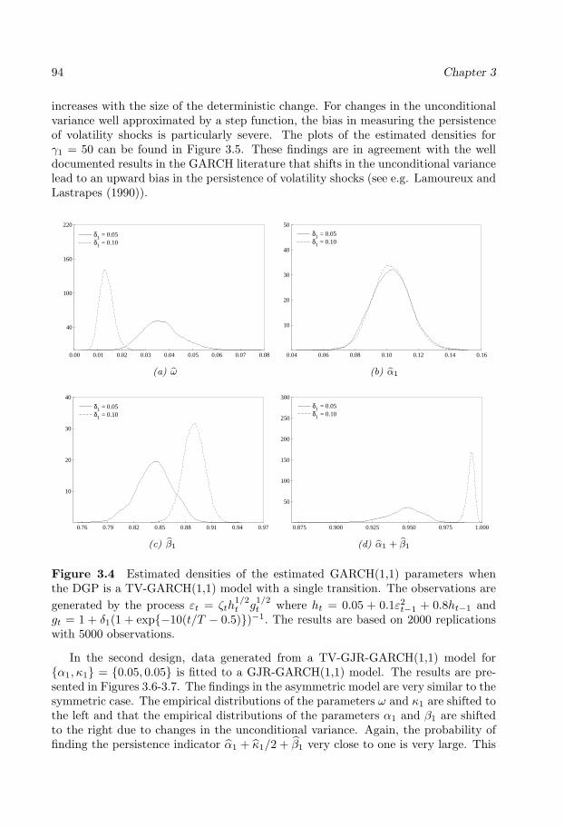
94 Chapter 3
increases with the size of the deterministic change. For changes in the unconditionalvariance well approximated by a step function, the bias in measuring the persistenceof volatility shocks is particularly severe. The plots of the estimated densities forγ1 = 50 can be found in Figure 3.5. These findings are in agreement with the welldocumented results in the GARCH literature that shifts in the unconditional variancelead to an upward bias in the persistence of volatility shocks (see e.g. Lamoureux andLastrapes (1990)).
0.00 0.01 0.02 0.03 0.04 0.05 0.06 0.07 0.08
40
100
160
220
δ1 = 0.05 δ1 = 0.10
(a) ω
0.04 0.06 0.08 0.10 0.12 0.14 0.16
10
20
30
40
50
δ1 = 0.05 δ1 = 0.10
(b) α1
0.76 0.79 0.82 0.85 0.88 0.91 0.94 0.97
10
20
30
40
δ1 = 0.05 δ1 = 0.10
(c) β1
0.875 0.900 0.925 0.950 0.975 1.000
50
100
150
200
250
300
δ1 = 0.05 δ1 = 0.10
(d) α1 + β1
Figure 3.4 Estimated densities of the estimated GARCH(1,1) parameters whenthe DGP is a TV-GARCH(1,1) model with a single transition. The observations aregenerated by the process εt = ζth
1/2t g
1/2t where ht = 0.05 + 0.1ε2t−1 + 0.8ht−1 and
gt = 1 + δ1(1 + exp{−10(t/T − 0.5)})−1. The results are based on 2000 replicationswith 5000 observations.
In the second design, data generated from a TV-GJR-GARCH(1,1) model for{α1, κ1} = {0.05, 0.05} is fitted to a GJR-GARCH(1,1) model. The results are pre-sented in Figures 3.6-3.7. The findings in the asymmetric model are very similar to thesymmetric case. The empirical distributions of the parameters ω and κ1 are shifted tothe left and that the empirical distributions of the parameters α1 and β1 are shiftedto the right due to changes in the unconditional variance. Again, the probability offinding the persistence indicator α1 + κ1/2 + β1 very close to one is very large. This

Modelling Changes in the Unconditional Variance 95
0.00 0.01 0.02 0.03 0.04 0.05 0.06 0.07 0.08
40
100
160
220
δ1 = 0.05 δ1 = 0.10
(a) ω
0.04 0.06 0.08 0.10 0.12 0.14 0.16
10
20
30
40
50
δ1 = 0.05 δ1 = 0.10
(b) α1
0.76 0.79 0.82 0.85 0.88 0.91 0.94 0.97
10
20
30
40
δ1 = 0.05 δ1 = 0.10
(c) β1
0.875 0.900 0.925 0.950 0.975 1.000
50
100
150
200
250
300
δ1 = 0.05 δ1 = 0.10
(d) α1 + β1
Figure 3.5 Estimated densities of the estimated GARCH(1,1) parameters whenthe DGP is a TV-GARCH(1,1) model with a single transition. The observations aregenerated by the process εt = ζth
1/2t g
1/2t where ht = 0.05 + 0.1ε2t−1 + 0.8ht−1 and
gt = 1 + δ1(1 + exp{−50(t/T − 0.5)})−1. The results are based on 2000 replicationswith 5000 observations.
effect is more remarkable when the changes in the unconditional variance are abrupt.Moreover, the simulations agree with the results obtained in the application.
It may be of interest to investigate the behaviour of the LM-type tests involved inthe modelling strategy when the data has been generated by a long-memory process.For this purpose, we study the empirical power properties of the test statistic usingas data-generating process the FIGARCH model of Baillie, Bollerslev, and Mikkelsen(1996). In particular, the artificial series is generated according to a FIGARCH(1,d,1)model as follows:
εt = ζth1/2t , εt|Ft−1 ∼ N(0, ht)
[1− βL]ht = ω + [1− βL− φL(1− L)d]ε2t
where ω = 0.05, φ = 0.5 and β = 0.7. We use sample sizes of 1000, 2500 and 5000observations with 2000 replications. The actual rejection frequencies of the test at

96 Chapter 3
0.00 0.01 0.02 0.03 0.04 0.05 0.06 0.07 0.08
50
100
150
200δ1 = 0.05 δ1 = 0.10
(a) ω
0.00 0.02 0.04 0.06 0.08 0.10 0.12
10
20
30
40
50δ1 = 0.05 δ1 = 0.10
(b) α1
0.01 0.03 0.05 0.07 0.09 0.11 0.13 0.15 0.17
5
10
15
20
25
30δ1 = 0.05 δ1 = 0.10
(c) κ1
0.75 0.77 0.79 0.81 0.83 0.85 0.87 0.89 0.91 0.93 0.95
10
20
30
40δ1 = 0.05 δ1 = 0.10
(d) β1
0.89 0.91 0.93 0.95 0.97 0.99 1.01
20
60
100
140
180
220δ1 = 0.05 δ1 = 0.10
(e) α1 + κ1/2 + β1
Figure 3.6 Estimated densities of the estimated GJR-GARCH(1,1) parameters whenthe DGP is a TV-GJR-GARCH(1,1) model with a single transition. The observa-tions are generated by the process εt = ζth
1/2t g
1/2t where ht = 0.05 + 0.05ε2t−1 +
0.1ε2t−1It−1(εt−1 < 0) + 0.8ht−1 and gt = 1 + δ1(1 + exp{−10(t/T − 0.5)})−1. Theresults are based on 2000 replications with 5000 observations.
1% and 5% critical values are reported in Table 3.8. Since we focus on the powerresults when the long-memory parameter d is located in the nonstationary region weuse d = 0.5, 0.6, 0.7 and 0.8. The power of the tests is moderate for the LM1−typetest for the sample size of 2500 observations. The LM3−type test is, however, morepowerful than the LM1−test and it has better power properties for the larger samplesize. Interestingly, the power is higher at low values of the long memory parameter dit is at higher values of this parameter.
3.6 Conclusions
In this paper we develop a testing and modelling procedure for describing the long-term movements in stock market returns over very long time periods. This is doneby multiplicatively decomposing the variance of a GARCH model into a conditionaland an unconditional component, in which the unconditional variance is allowed tochange smoothly over time. The proposed model is the Time-Varying GARCH modelas in Amado and Terasvirta (2008). The model building strategy relies on statisticalinference, making use of a sequence of Lagrange-multiplier type specification tests.Because of the length of the observation period, the time series is divided into non-overlapping subperiods with the aim of alleviating the model building procedure. One

Modelling Changes in the Unconditional Variance 97
0.00 0.01 0.02 0.03 0.04 0.05 0.06 0.07 0.08
50
100
150
200δ1 = 0.05 δ1 = 0.10
(a) ω
0.00 0.02 0.04 0.06 0.08 0.10 0.12
10
20
30
40
50δ1 = 0.05 δ1 = 0.10
(b) α1
0.01 0.03 0.05 0.07 0.09 0.11 0.13 0.15 0.17
5
10
15
20
25
30δ1 = 0.05 δ1 = 0.10
(c) κ1
0.75 0.77 0.79 0.81 0.83 0.85 0.87 0.89 0.91 0.93 0.95
10
20
30
40δ1 = 0.05 δ1 = 0.10
(d) β1
0.89 0.91 0.93 0.95 0.97 0.99 1.01
20
60
100
140
180
220δ1 = 0.05 δ1 = 0.10
(e) α1 + κ1/2 + β1
Figure 3.7 Estimated densities of the estimated GJR-GARCH(1,1) parameters whenthe DGP is a TV-GJR-GARCH(1,1) model with a single transition. The observa-tions are generated by the process εt = ζth
1/2t g
1/2t where ht = 0.05 + 0.05ε2t−1 +
0.1ε2t−1It−1(εt−1 < 0) + 0.8ht−1 and gt = 1 + δ1(1 + exp{−50(t/T − 0.5)})−1. Theresults are based on 2000 replications with 5000 observations.
Table 3.8 Actual rejection frequencies of the standard LM test of constant uncon-ditional variance
d = 0.5 d = 0.6 d = 0.7 d = 0.8α LM1 LM3 LM1 LM3 LM1 LM3 LM1 LM3
T = 1000 1% 18.20 27.80 19.55 29.75 18.70 28.90 14.80 23.805% 33.15 48.35 33.85 50.45 31.90 48.85 27.30 41.95
T = 2500 1% 29.85 49.20 29.60 49.80 25.95 45.40 19.20 35.155% 45.25 67.55 44.75 68.40 38.30 62.10 30.40 53.50
T = 5000 1% 37.65 66.30 35.50 64.85 28.95 54.05 20.50 38.005% 50.95 78.80 48.15 76.25 42.45 69.65 32.65 56.00
Notes: Monte Carlo results in percentage of the non-robust LM parameter constancy testbased on 2000 replications. The artificial series is generated according to a FIGARCH(1,d,1)model yt = εt, εt|Ft−1 ∼ N(0, ht) and [1 − βL]ht = ω + [1 − βL − φL(1 − L)d]ε2t . Resultsare shown for the LM test at the 1%, 5% and 10% nominal significance levels. The columns‘LM1’ and ‘LM3’ correspond to the test procedure based on the first-order and third-orderTaylor expansions, respectively.

98 Chapter 3
advantage of this device is that it provides a modelling framework particularly usefulin applications involving very long time series.
An empirical example applied to the long daily DJIA return series shows howthe technique works in practice. Our results show that the dependence structure ofthe series is best explained by deterministic changes in the unconditional variance,and consequently the hypothesis of constant unconditional variance turns out to beinappropriate. We also show empirically and with a small Monte Carlo experimenthow unmodelled deterministic changes in the unconditional variance reproduce thelong-memory property in the variance. Based on the diagnostic tests, we claim thatthe nonstationary TV-GARCH model should be preferred to the stationary model inapplications using long financial data.
Moreover, the results indicate that the first-order GJR-GARCH model is inad-equate to describe the short-run dynamics of volatility over long return series, andanother type of nonlinear model should be considered. Further improvements in themodelling of the conditional variance over long time series are needed, but this prob-lem is left for further research.

Appendix A: Figures 99
Appendix A: Figures
0 500 1000 1500 2000 2500 3000
0.5
1.0
1.5
2.0
2.5
3.0
3.5
(a) Subperiod 1
3000 3500 4000 4500 5000 5500 6000
0.2
0.4
0.6
0.8
1.0
1.2
(b) Subperiod 2
6000 6500 7000 7500 8000 8500 9000 9500 10000 10500
0.75
0.80
0.85
0.90
0.95
1.00
(c) Subperiod 3
10750 11750 12750 13750 14750 15750
1.0
1.5
2.0
2.5
3.0
(d) Subperiod 4
18600 19100 19600 20100 20600 21100
1.1
1.4
1.7
2.0
2.3
(e) Subperiod 6
Figure 3.8 Estimated gt functions for the five subperiods.

100 Chapter 3
0 500 1000 1500 2000 2500 3000
1
2
3
4
5
6
7
8GJR−GARCH(1,1) TV−GJR−GARCH(1,1)
(a) Subperiod 1
3000 3500 4000 4500 5000 5500 6000
1
2
3
4
5
6
7
8GJR−GARCH(1,1) TV−GJR−GARCH(1,1)
(b) Subperiod 2
6000 6500 7000 7500 8000 8500 9000 9500 10000 10500
1.0
1.5
2.0
2.5
3.0GJR−GARCH(1,1) TV−GJR−GARCH(1,1)
(c) Subperiod 3
10750 11750 12750 13750 14750 15750
0.5
1.0
1.5
2.0
2.5
3.0GJR−GARCH(1,1) TV−GJR−GARCH(1,1)
(d) Subperiod 4
18600 19100 19600 20100 20600 21100
1
2
3
4GJR−GARCH(1,1) TV−GJR−GARCH(1,1)
(e) Subperiod 6
Figure 3.9 Conditional standard deviations of the GJR-GARCH(1,1) and the TV-GJR-GARCH(1,1) model for the five subperiods.

Appendix B: Tables 101
Appendix B: Tables
Table 3.9 Summary statistics of the subperiod return seriesPeriods Min Max Mean S.D. Skew Ex.Kr. Rob.Sk. Rob.Kr.
Subsample 1 (02/01/1920 − 31/12/1931): T=3004
εt -14.47 13.86 -0.011 1.486 -0.402 13.97 -0.073 0.173
εt/g1/2t -5.669 4.704 0.017 0.876 -0.435 2.899 -0.030 0.118
Subsample 2 (04/01/1932 − 31/12/1943): T=2995
εt -8.778 14.27 0.019 1.652 0.198 7.178 -0.015 0.389
εt/g1/2t -4.785 5.824 0.011 0.860 -0.173 3.684 0.008 0.266
Subsample 3 (04/01/1944 − 29/12/1961): T=4511
εt -6.766 4.048 0.037 0.702 -0.869 6.378 0.008 0.145
εt/g1/2t -6.766 4.048 0.036 0.660 -0.818 6.054 0.013 0.143
Subsample 4 (01/01/1962 − 16/11/1982): T=5241
εt -5.882 4.952 0.006 0.844 0.251 2.908 -0.015 0.123
εt/g1/2t -5.878 4.576 0.005 0.656 0.185 3.822 -0.002 0.068
Subsample 5 (17/11/1982 − 31/12/1993): T=2813
εt -25.63 9.666 0.047 1.087 -4.768 115.57 -0.020 0.187Subsample 6 (03/01/1994 − 31/12/2003): T=2557
εt -7.455 6.155 0.040 1.111 -0.261 4.131 0.030 0.232
εt/g1/2t -5.655 4.262 0.033 0.814 -0.287 3.653 0.040 0.148
Notes: The table contains summary statistics for each of the subperiod series. The sample periodsare indicated in parentheses. The statistic ‘S.D.’ is the standard deviation, ‘Skew’ is the coefficientof skewness and the statistic ‘Ex.Kr’ is the value of the excess kurtosis. ‘Rob.Sk.’ denotes therobust measure for skewness and ‘Rob.Kr.’ denotes the robust centred coefficient for kurtosis.‘Rob.Sk.’ is computed as SK = (Q3 +Q1 − 2Q2)/(Q3 −Q1) where Qi is the i th quartile of thereturns and ‘Rob.Kr.’ is computed as KR = (E7 − E5 + E3 − E1)/(E6 − E2)− 1.23 where Ei isthe i th octile (see Kim and White (2004) for details).

102 Chapter 3
Table 3.10 Estimation results of the TV-GJR-GARCH(1,1) model: subperiods
Subsample 1
ht = 0.0668(0.0223)
+ 0.0032(0.0132)
ε∗2t−1 + 0.8244(0.0405)
ht−1 + 0.1575(0.0383)
It−1(ε∗t−1 < 0)ε∗2t−1
Log-Lik = −3677.8 α1 + β1 + κ1/2 = 0.9063
gt = 0.3738(0.0128)
+ 0.4779(0.0627)
(1 + exp{−24.379(8.3423)
(t∗ − 0.0856(0.0036)
)(t∗ − 0.7228(0.0118)
)})−1
+2.3966(0.2051)
(1 + exp{−100(−)
(t∗ − 0.8109(0.0023)
)})−1
Subsample 2
ht = 0.0205(0.0065)
+ 0.0338(0.0098)
ε∗2t−1 + 0.8876(0.0220)
ht−1 + 0.1041(0.0277)
It−1(ε∗t−1 < 0)ε∗2t−1
Log-Lik = −3524.3 α1 + β1 + κ1/2 = 0.9735
gt = 1.1331(0.0585)
− 0.7717(0.0599)
(1 + exp{−100(−)
(t∗ − 0.2128(0.0031)
)})−1
−0.2130(0.0152)
(1 + exp{−100(−)
(t∗ − 0.7395(0.0020)
)})−1
Subsample 3
ht = 0.0423(0.0255)
+ 0.0007(0.0109)
ε∗2t−1 + 0.8331(0.0793)
ht−1 + 0.1348(0.05278)
It−1(ε∗t−1 < 0)ε∗2t−1
Log-Lik = −4298.5 α1 + β1 + κ1/2 = 0.9012
gt = 1− 0.2369(0.0207)
(1 + exp{−100(−)
(t∗ − 0.3937(0.0039)
)})−1
Subsample 4
ht = 0.0076(0.0016)
+ 0.0203(0.0056)
ε∗2t−1 + 0.9191(0.0094)
ht−1 + 0.0884(0.0116)
It−1(ε∗t−1 < 0)ε∗2t−1
Log-Lik = −4769.2 α1 + β1 + κ1/2 = 0.9836
gt = 1 + 2.4727(0.2498)
(1 + exp{−14.373(4.9947)
(t∗ − 0.5568(0.0059)
)})−1
−1.4488(0.2590)
(1 + exp{−100(−)
(t∗ − 0.6775(0.0040)
)})−1
Subsample 6
ht = 0.0197(0.0065)
+ 0.9026(0.0225)
ht−1 + 0.1400(0.0341)
It−1(ε∗t−1 < 0)ε∗2t−1
Log-Lik = −2883.1 α1 + β1 + κ1/2 = 0.9726
gt = 1 + 1.0949(0.0741)
(1 + exp{−8.3780(9.5905)
(t∗ − 0.2967(0.0128)
)})−1
Notes: The table contains the parameter estimates from the TV-GJR(1,1) model foreach of the subperiods of the DJIA daily returns from January 2, 1920 until December31, 2003. The estimated model has the form of the equations (3.5)-(3.8). The numbersin parentheses are the standard errors.

Appendix B: Tables 103
Table 3.11 Estimation results of the GJR-GARCH(1,1) model: subperiods
Subsample 1
ht = 0.0467(0.0110)
+ 0.0230(0.0093)
ε∗2t−1 + 0.8752(0.0176)
ht−1 + 0.1399(0.0255)
It−1(ε∗t−1 < 0)ε∗2t−1
Log-Lik = −4675.49 α1 + β1 + κ1/2 = 0.9680
Subsample 2
ht = 0.0168(0.0063)
+ 0.0349(0.0111)
ε∗2t−1 + 0.9126(0.0192)
ht−1 + 0.0930(0.0260)
It−1(ε∗t−1 < 0)ε∗2t−1
Log-Lik = −4911.1 α1 + β1 + κ1/2 = 0.9940
Subsample 3
ht = 0.0332(0.0274)
+ 0.0015(0.0105)
ε∗2t−1 + 0.8732(0.0881)
ht−1 + 0.1111(0.0642)
It−1(ε∗t−1 < 0)ε∗2t−1
Log-Lik = −4542.8 α1 + β1 + κ1/2 = 0.9302
Subsample 4
ht = 0.0045(0.0012)
+ 0.0252(0.0055)
ε∗2t−1 + 0.9310(0.0077)
ht−1 + 0.0814(0.0110)
It−1(ε∗t−1 < 0)ε∗2t−1
Log-Lik = −5908.2 α1 + β1 + κ1/2 = 0.9969
Subsample 5
ht = 0.0359(0.0313)
+ 0.0279(0.0136)
ε∗2t−1 + 0.8932(0.0633)
ht−1 + 0.0941(0.0799)
It−1(ε∗t−1 < 0)ε∗2t−1
Log-Lik = −3736.4 α1 + β1 + κ1/2 = 0.9681
Subsample 6
ht = 0.0189(0.0062)
+ 0.0059(0.0095)
ε∗2t−1 + 0.9169(0.0177)
ht−1 + 0.1299(0.0313)
It−1(ε∗t−1 < 0)ε∗2t−1
Log-Lik = −3587.5 α1 + β1 + κ1/2 = 0.9878
Notes: The table contains the parameter estimates from the GJR(1,1) model for eachof the subperiods of the DJIA daily returns from January 2, 1920 until December31, 2003. The estimated model has the form hit = ωi + αi1ε
2it−1 + βi1hit−1 +
κi1Iit−1(εit−1)ε2it−1, where Iit(εit) = 1 if εit < 0 (and 0 otherwise) for all i. Thenumbers in parentheses are the Bollerslev-Wooldridge robust standard errors.

104 Chapter 3
Table 3.12 GPH estimates of the long-memory parameter
dGPH(m = T 0.4) dGPH(m = T 0.5) dGPH(m = T 0.6)
Periods εt εt/g1/2t εt εt/g
1/2t εt εt/g
1/2t
Subsample 1 0.3688(0.1434)
−0.171(0.1214)
0.4237(0.0866)
0.1059(0.0837)
0.4050(0.0539)
0.2001(0.04865)
Subsample 2 0.7285(0.1199)
0.2173(0.1918)
0.6442(0.0889)
0.2924(0.1035)
0.5240(0.0651)
0.3725(0.0683)
Subsample 3 0.2958(0.1618)
0.2454(0.1493)
0.3134(0.0885)
0.2892(0.0836)
0.2898(0.0466)
0.2802(0.0454)
Subsample 4 0.4457(0.1330)
0.2228(0.1179)
0.4728(0.0893)
0.3198(0.0773)
0.4873(0.0605)
0.4333(0.0520)
Subsample 5 0.2996(0.0974)
0.2996(0.0974)
0.4420(0.0819)
0.4420(0.0819)
0.2902(0.0446)
0.2902(0.0446)
Subsample 6 0.4776(0.1543)
0.3804(0.1820)
0.4250(0.0924)
0.3552(0.0968)
0.4015(0.0551)
0.3515(0.0572)
Notes: The numbers in parentheses are the standard errors. The bandwidth mequals Tα, α ∈ {0.4, 0.5, 0.6} where T is the number of observations.
Bibliography
Amado, C., and T. Terasvirta (2008): “Modelling Unconditional and ConditionalHeteroskedasticity with Smoothly Time-Varying Structure,” SSE/EFI Working Pa-per Series in Economics and Finance No. 691.
Baillie, R. T., T. Bollerslev, and H. O. Mikkelsen (1996): “FractionallyIntegrated Generalized Autoregressive Conditional Heteroskedasticity,” Journal ofEconometrics, 74, 3–30.
Baillie, R. T., and C. Morana (2007): “Modeling Long Memory and StructuralBreaks in Conditional Variances: An Adaptive FIGARCH Approach,” WorkingPaper No. 593, Queen Mary University of London, Department of Economics.
Bollerslev, T. (1986): “Generalized Autoregressive Conditional Heteroskedastic-ity,” Journal of Econometrics, 31, 307–327.
Diebold, F. X. (1986): “Comment on ”Modelling the Persistence of ConditionalVariance”, by R. Engle and T. Bollerslev,” Econometric Reviews, 5, 51–56.
Doornik, J. A. (2002): Object-Oriented Matrix Programming Using Ox. TimberlakeConsultants Press, see also www.nuff.ox.ac.uk/Users/Doornik, 3rd edn.
Engle, R. F., and J. Gonzalo Rangel (2008): “The Spline-GARCH Model forLow-Frequency Volatility and its Global Macroeconomic Causes,” Review of Fi-nancial Studies, 21, 1187–1222.
Engle, R. F., and G. G. J. Lee (1999): “A Long-Run and Short-Run ComponentModel of Stock Return Volatility,” in Cointegration, Causality, and Forecasting: AFestschrift in Honour of Clive W. J. Granger, ed. by R. F. Engle, and H. White,pp. 475–497. Oxford University Press.
Fiorentini, G., G. Calzolari, and L. Panattoni (1996): “Analytic Derivativesand the Computation of GARCH Estimates,” Journal of Applied Econometrics,11, 399–417.
Gallant, R. (1984): “The Fourier Flexible Form,” American Journal of AgriculturalEconomics, 66, 204–208.
105

106 Bibliography
Geweke, J., and S. Porter-Hudak (1983): “The Estimation and Application ofLong-Memory Time-Series Models,” Journal of Time Series Analysis, 4, 221–238.
Glosten, L. R., R. Jagannathan, and D. E. Runkle (1993): “On the RelationBetween the Expected Value and the Volatility of the Nominal Excess Return onStocks,” The Journal of Finance, 48, 1779–1801.
Granger, C. W. J., and N. Hyung (2004): “Occasional Structural Breaks andLong Memory with an Application to the SP 500 Absolute Stock Returns,” Journalof Empirical Finance, 11, 399–421.
Kim, T.-H., and H. White (2004): “On More Robust Estimation of Skewness andKurtosis,” Finance Research Letters, 1, 56–73.
Lamoureux, C. G., and W. D. Lastrapes (1990): “Persistence in Variance, Struc-tural Change, and the GARCH Model,” Journal of Business & Economic Statistics,8, 225–234.
Luukkonen, R., P. Saikkonen, and T. Terasvirta (1988): “Testing LinearityAgainst Smooth Transition Autoregressive Models,” Biometrika, 75, 491–499.
Mikosch, T., and C. Starica (2004): “Nonstationarities in Financial Time Series,the Long-Range Dependence, and the IGARCH Effects,” The Review of Economicsand Statistics, 86, 378–390.
Song, P. X., Y. Fan, and J. D. Kalbfleisch (2005): “Maximization by Parts inLikelihood Inference,” Journal of the American Statistical Association, 100, 1145–1158.
Starica, C., and C. W. J. Granger (2005): “Nonstationarities in Stock Returns,”Review of Economics and Statistics, 87, 503–522.

Chapter 4
Conditional CorrelationModels of AutoregressiveConditionalHeteroskedasticity withNonstationary GARCHEquations
107


109
Conditional Correlation Models of Autoregressive
Conditional Heteroskedasticity with Nonstationary
GARCH Equations 1
Abstract
In this paper we investigate the effects of careful modelling the long-run dynamicsof the volatilities of stock market returns on the conditional correlation structure.To this end we allow the individual unconditional variances in Conditional Correla-tion GARCH models to change smoothly over time by incorporating a nonstationarycomponent in the variance equations. The modelling technique to determine theparametric structure of this time-varying component is based on a sequence of speci-fication Lagrange multiplier-type tests derived in Amado and Terasvirta (2008). Thevariance equations combine the long-run and the short-run dynamic behaviour of thevolatilities. The structure of the conditional correlation matrix is assumed to be ei-ther time independent or to vary over time. We apply our model to pairs of sevendaily stock returns belonging to the S&P 500 composite index and traded at the NewYork Stock Exchange. The results suggest that accounting for deterministic changesin the unconditional variances considerably improves the fit of the multivariate Con-ditional Correlation GARCH models to the data. The effect of careful specification ofthe variance equations on the estimated correlations is variable: in some cases rathersmall, in others more discernible.
1This paper is a joint work with Timo Terasvirta.Acknowledgements: The first author would like to acknowledge financial support from the
Louis Fraenckels Stipendiefond. Part of this research was done while the first author was visitingCREATES, University of Aarhus, whose kind hospitality is gratefully acknowledged. The Centerfor Research in Econometric Analysis of Time Series, CREATES, is funded by the Danish NationalResearch Foundation. The responsibility for any errors and shortcomings in this paper remains ours.
110 Chapter 4
4.1 Introduction
Many financial issues, such as hedging and risk management, portfolio selection andasset allocation rely on information about the covariances or correlations between theunderlying returns. This has motivated the modelling of volatility using multivariatefinancial time series rather than modelling individual returns separately. A numberof multivariate generalized autoregressive conditional heteroskedasticity (GARCH)models have been proposed, and some of them have become standard tools for financialanalysts. For recent surveys of Multivariate GARCH models see Bauwens, Laurent,and Rombouts (2006) and Silvennoinen and Terasvirta (2008).
In the univariate setting, volatility models have been extensively investigated.Many modelling proposals of univariate financial returns have suggested that non-stationarities in return series may cause the extreme persistence of shocks observedthrough estimated GARCH models. In particular, Mikosch and Starica (2004) foundthat the long-range dependence and the ‘integrated GARCH effect’ can also be ex-plained by unaccounted structural breaks in the unconditional variance. Previously,Diebold (1986) and Lamoureux and Lastrapes (1990) have also argued that spuriouslong memory may be detected from a time series with structural breaks.
The problem of structural breaks in the conditional variance can be tackled byintroducing nonstationarity in the volatility equations. In the univariate context,Dahlhaus and Subba Rao (2006) proposed a locally time-varying ARCH processfor modelling nonstationary. Engle and Gonzalo Rangel (2008) and, independently,Amado and Terasvirta (2008) proposed an approach in which the volatility is mod-elled by a multiplicative decomposition of both conditional and unconditional vari-ance. More specifically, the unconditional variance component is modelled by a slowlyvarying function: Engle and Gonzalo Rangel (2008) used an exponential spline for thispurpose. As an alternative, Amado and Terasvirta (2008) described the nonstationarycomponent of volatility by a linear combination of logistic transition functions. Theauthors proposed a modelling technique for determining the parametric structure ofthe time-varying component from the data.
Despite the growing literature on multivariate GARCH models, little attentionhas been devoted to modelling multivariate financial data by explicitly allowing fornonstationarity. Recently, Hafner and Linton (2008) proposed a semiparametric gen-eralization of the scalar multiplicative model of Engle and Gonzalo Rangel (2008).Their multivariate GARCH model is a first-order BEKK model with a deterministicnonstationary component. The authors suggested an estimation procedure for theparametric and nonparametric components and established semiparametric efficiencyof their estimators.
In this paper, we propose a parametric extension of the univariate multiplicativeGARCH model of Amado and Terasvirta (2008) to the multivariate case. We investi-gate the effects of careful modelling of the time-varying unconditional variance on thecorrelation structure in Conditional Correlation GARCH (CC-GARCH) models. Tothis end, we allow the individual unconditional variances in the multivariate GARCHmodels to change smoothly over time by incorporating a nonstationary componentin the variance equations. The empirical analysis consists of fitting bivariate con-

Conditional Correlations Models with Nonstationary GARCH Equations 111
ditional correlation GARCH models to pairs of daily return series and comparingthe results from models with the time-varying unconditional variance component tomodels without such a component. As a by-product, we extend the concept of newsimpact surfaces of Kroner and Ng (1998) to the case where both the variances andconditional correlations are fluctuating over time. These surfaces illustrate how theimpact of news to covariances between asset returns depends both on the state of themarket and the time-varying dependence between the returns.
This paper is organized as follows. In Section 4.2 we describe the ConditionalCorrelation GARCH model in which the individual unconditional variances changesmoothly over time. Estimation of parameters of these models is discussed in Section4.3. Details regarding the modelling strategy are considered in Section 4.4. Section4.5 contains the empirical results of fitting bivariate CC-GARCH models to 21 pairs ofseven daily stock return series belonging to the S&P 500 composite index. Conclusionscan be found in Section 4.6.
4.2 The model
4.2.1 The general framework
Consider a N × 1 vector of return time series {yt}, t = 1, . . . , T, described by thefollowing vector process:
yt = E(yt|Ft−1) + εt (4.1)
where Ft−1 is the sigma-algebra generated by the available information up until t−1.For simplicity, we assume that the conditional expectation of the returns E(yt|Ft−1) =0. The N−dimensional vector of innovations (or returns) {εt} is defined as
εt = Σ1/2t ζt (4.2)
where the conditional covariance matrix Σt = [σijt] of εt, given the informationset Ft−1, is a positive-definite N × N matrix. The error vectors ζt form a se-quence of independent and identically distributed variables with mean zero and apositive definite correlation matrix Pt. Furthermore, the vector of standardized er-rors P−1/2
t ζt ∼ iid(0, IN ). Under these assumptions, the error vector εt satisfies thefollowing moments conditions:
E(εt|Ft−1) = 0
E(εtε′t|Ft−1) = Σt = DtPtD′t (4.3)
where Dt is a diagonal matrix of standard deviations. It is now assumed that Dt con-sists of a conditionally heteroskedastic component and a deterministic time-dependentone such that
Dt = StGt (4.4)
where St = diag(h1/21t , . . . , h
1/2Nt ) contains the conditional standard deviations h1/2
it , i =1, . . . , N, and Gt = diag(g1/2
1t , . . . , g1/2Nt ). The elements git, i = 1, . . . , N, are positive-
valued deterministic functions of time, whose structure will be defined in a moment.

112 Chapter 4
Equations (4.3) and (4.4) jointly define the time-varying covariance matrix
Σt = StGtPtGtSt. (4.5)
It follows thatσijt = ρijt(hitgit)1/2(hjtgjt)1/2, i 6= j (4.6)
and thatσiit = hitgit, i = 1, . . . , N. (4.7)
From (4.7) it follows that hit = σiit/git = E(ε∗itε∗′it |Ft−1), where ε∗it = εit/g
1/2it . When
Gt ≡ IN and the conditional correlation matrix Pt ≡ P, these assumptions define theConstant Conditional Correlation (CCC-) GARCH model of Bollerslev (1990). Moregenerally, when Gt ≡ IN and Pt is a time-varying correlation matrix, the modelbelongs to the family of Conditional Correlation GARCH models.
The diagonal elements of the matrix Gt are defined as follows:
git = 1 +r∑l=1
δilGil(t/T ; γil, cil) (4.8)
with γil > 0, i = 1, . . . , N, l = 1, . . . , r. Each git varies smoothly over time satisfyingthe conditions inf
t=1,...,Tgit > 0, and δil ≤ Mδ < ∞, l = 1, . . . , r, for i = 1, . . . , N.
The parametric form of (4.8), introduced in Amado and Terasvirta (2008), allows theunconditional variance to change smoothly over time according to the transition func-tion Gil(t/T ; γil, cil). The function Gil(t/T ; γil, cil) is a generalized logistic function,that is,
Gil(t/T ; γil, cil) =
1 + exp
−γilk∏j=1
(t/T − cilj)
−1
, γil > 0, cil1 ≤ ... ≤ cilk.
(4.9)Function (4.9) is by construction continuous and bounded between zero and one.The parameters, cilj and γil, determine the location and the speed of the transitionbetween regimes.
The parametric form of (4.8) with (4.9) is very flexible and capable of describingsmooth deterministic changes in volatility. Under δi1 = ... = δir = 0, i = 1, . . . , N, in(4.8), the unconditional volatility becomes constant. Assuming either r > 1 or k > 1or both with δil 6= 0 adds flexibility to the unconditional variance component git. Inthe simplest case, r = 1 and k = 1, git increases monotonically over time when δil > 0and decreases monotonically when δil < 0. The slope parameter γi1 in (4.9) controlsthe degree of smoothness of the transition: the larger γi1, the faster the transition isbetween the extreme regimes. As γi1 →∞, git approaches a step function. For smallvalues of γi1, the transition between regimes is very smooth.
In this work we shall account for potentially asymmetric responses of volatility topositive and negative shocks or returns by modelling the conditional variances by the

Conditional Correlations Models with Nonstationary GARCH Equations 113
GJR-GARCH process of Glosten, Jagannathan, and Runkle (1993). In the presentcontext,
hit = ωi +q∑j=1
αijε∗2i,t−j +
q∑j=1
κijI(ε∗i,t−j < 0)ε∗2i,t−j +p∑j=1
βijhi,t−j , (4.10)
where the indicator function I(A) = 1 when A is valid, otherwise I(A) = 0.
4.2.2 The structure of the conditional correlations
In this work we shall investigate the effects of modelling changes in the unconditionalvariances on conditional correlations. The idea is to compare models in which thenonstationary component is left unmodelled with ones relying on the decomposition(4.5) with Gt 6= IN . As to modelling the time-variation in the correlation matrixPt, several choices exist. As already mentioned, the simplest multivariate correlationmodel is the CCC-GARCH model in which Pt ≡ P. With hit specified as in (4.10),this model will be called the CCC-TVGJR-GARCH model. When git ≡ 1, (4.10)defines the ith conditional variance of the CCC-GJR-GARCH model.
The CCC-GARCH model has considerable appeal due to its computational sim-plicity, but in many studies the assumption of constant correlations has been found tobe too restrictive. There are several ways of relaxing this assumption using parametricrepresentations for the correlations. Engle (2002) introduced the so-called DynamicCC-GARCH (DCC-GARCH) model in which the conditional correlations are definedthrough GARCH(1,1) type equations. Tse and Tsui (2002) presented a rather similarmodel. In the DCC-GARCH model, the coefficient of correlation ρijt is a typicalelement of the matrix Pt with the dynamic structure
Pt = {diagQt}−1/2Qt{diagQt}−1/2 (4.11)
whereQt = (1− θ1 − θ2)Q + θ1ζt−1ζ
′t−1 + θ2Qt−1 (4.12)
with the scalars θ1 and θ2 satisfying θ1 > 0 and θ2 ≥ 0 such that θ1 + θ2 < 1,Q isthe unconditional correlation matrix of the standardized errors ζit, i = 1, . . . , N, andζt = (ζ1t, . . . , ζNt)′. In our case, each ζit = εit/(hitgit)1/2, and this version of themodel will be called the DCC-TVGJR-GARCH model. Accordingly, when git ≡ 1,the model becomes the DCC-GJR-GARCH model.
Another way of introducing time-varying correlations is to assume that the con-ditional correlation matrix Pt varies smoothly over time between two extreme statesof correlations P(1) and P(2); see Berben and Jansen (2005) and Silvennoinen andTerasvirta (2005, 2007). The correlation matrix is a convex combination of these twomatrices such that:
Pt = {1−G(st; γ, c)}P(1) +G(st; γ, c)P(2) (4.13)
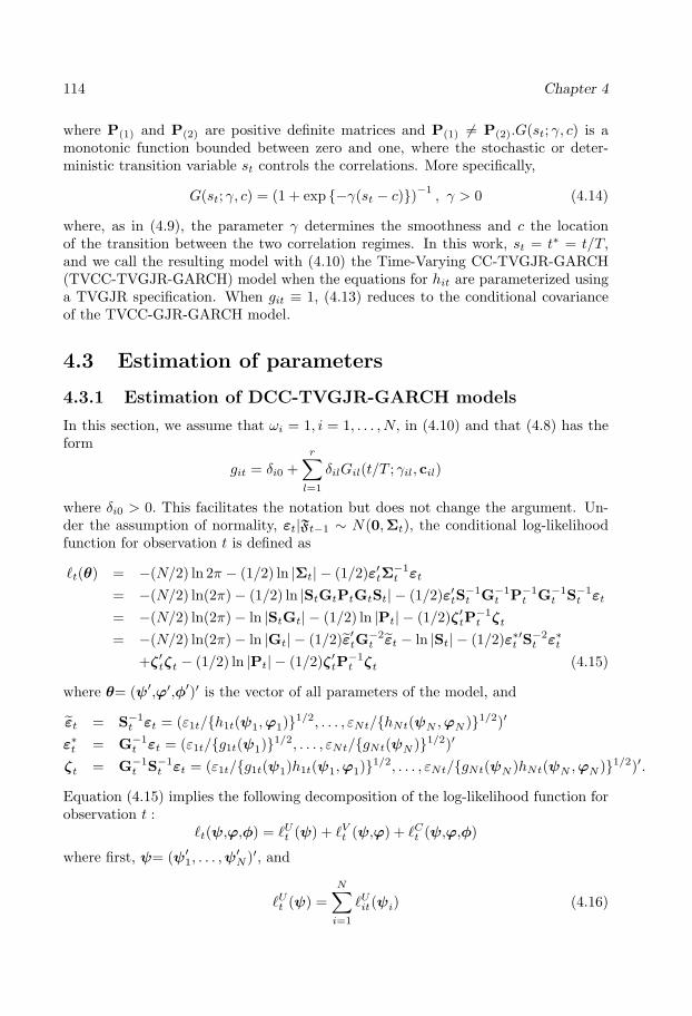
114 Chapter 4
where P(1) and P(2) are positive definite matrices and P(1) 6= P(2).G(st; γ, c) is amonotonic function bounded between zero and one, where the stochastic or deter-ministic transition variable st controls the correlations. More specifically,
G(st; γ, c) = (1 + exp {−γ(st − c)})−1, γ > 0 (4.14)
where, as in (4.9), the parameter γ determines the smoothness and c the locationof the transition between the two correlation regimes. In this work, st = t∗ = t/T,and we call the resulting model with (4.10) the Time-Varying CC-TVGJR-GARCH(TVCC-TVGJR-GARCH) model when the equations for hit are parameterized usinga TVGJR specification. When git ≡ 1, (4.13) reduces to the conditional covarianceof the TVCC-GJR-GARCH model.
4.3 Estimation of parameters
4.3.1 Estimation of DCC-TVGJR-GARCH models
In this section, we assume that ωi = 1, i = 1, . . . , N, in (4.10) and that (4.8) has theform
git = δi0 +r∑l=1
δilGil(t/T ; γil, cil)
where δi0 > 0. This facilitates the notation but does not change the argument. Un-der the assumption of normality, εt|Ft−1 ∼ N(0,Σt), the conditional log-likelihoodfunction for observation t is defined as
`t(θ) = −(N/2) ln 2π − (1/2) ln |Σt| − (1/2)ε′tΣ−1t εt
= −(N/2) ln(2π)− (1/2) ln |StGtPtGtSt| − (1/2)ε′tS−1t G−1
t P−1t G−1
t S−1t εt
= −(N/2) ln(2π)− ln |StGt| − (1/2) ln |Pt| − (1/2)ζ′tP−1t ζt
= −(N/2) ln(2π)− ln |Gt| − (1/2)ε′tG−2t εt − ln |St| − (1/2)ε∗′t S−2
t ε∗t
+ζ′tζt − (1/2) ln |Pt| − (1/2)ζ′tP−1t ζt (4.15)
where θ= (ψ′,ϕ′,φ′)′ is the vector of all parameters of the model, and
εt = S−1t εt = (ε1t/{h1t(ψ1,ϕ1)}1/2, . . . , εNt/{hNt(ψN ,ϕN )}1/2)′
ε∗t = G−1t εt = (ε1t/{g1t(ψ1)}1/2, . . . , εNt/{gNt(ψN )}1/2)′
ζt = G−1t S−1
t εt = (ε1t/{g1t(ψ1)h1t(ψ1,ϕ1)}1/2, . . . , εNt/{gNt(ψN )hNt(ψN ,ϕN )}1/2)′.
Equation (4.15) implies the following decomposition of the log-likelihood function forobservation t :
`t(ψ,ϕ,φ) = `Ut (ψ) + `Vt (ψ,ϕ) + `Ct (ψ,ϕ,φ)
where first, ψ= (ψ′1, . . . ,ψ′N )′, and
`Ut (ψ) =N∑i=1
`Uit(ψi) (4.16)

Conditional Correlations Models with Nonstationary GARCH Equations 115
withψi = (δi0, δ′i,γ′i, c′i)′, δi = (δi1, . . . , δir)′,γi = (γi1, . . . , γir)′, ci = (c′i1, . . . , c
′ir)′, i =
1, . . . , N, and`Uit(ψi) = −(1/2){ln git(ψi) + ε2it/git(ψi)}.
Second,
`Vt (ψ,ϕ) =N∑i=1
`Vit(ψi,ϕi) (4.17)
where ϕ= (ϕ′1, . . . ,ϕ′N )′, and
`Vit(ψi,ϕi) = −(1/2){lnhit(ψi,ϕi) + ε∗2it /hit(ψi,ϕi)}.
with ϕi = (αi1, . . . , αiq, κi1, . . . , κiq, βi1, . . . , βip)′, i = 1, . . . , N. Finally,
`Ct (ψ,ϕ,φ) = −(1/2){ln |Pt(ψ,ϕ,φ)|+ ζ′tP−1t (ψ,ϕ,φ)ζt − 2ζ′tζt}. (4.18)
The GARCH equations are estimated separately using maximization by parts.The first iteration consists of the following:
1. Maximize
LUiT (ψ) =T∑t=1
`Uit(ψ) = −(1/2)T∑t=1
{ln git(ψi) + ε2it/git(ψi)}
for each i, i = 1, . . . , N, separately, assuming εit = εit, that is, setting
hit(ψi,ϕi) ≡ 1. The resulting estimators are ψ(1)
i , i = 1, . . . , N.
2. Making use of ψ(1)
i , i = 1, . . . , N, maximize
LViT (ψ(1)
i ,ϕi) =T∑t=1
`Vit(ψ(1)
i ,ϕi) = −(1/2)T∑t=1
{lnhit(ψ(1)
i ,ϕi)+ε∗2it /hit(ψ
(1)
i ,ϕi)}
with respect to ϕi assuming ε∗it = εit/g1/2it (ψ
(1)
i ), for each i, i = 1, . . . , N, sepa-rately. Call the resulting estimators ϕ(1)
i , i = 1, . . . , N.
The second iteration is as follows:
1. Maximize
LUiT (ψ) =T∑t=1
`Uit(ψi) = −(1/2)T∑t=1
{ln git(ψi) + ε2it/git(ψi)}
assuming εit = εit/h1/2it (ψ
(1)
i , ϕ(1)i ), for each i, i = 1, . . . , N. Call the resulting
estimators ψ(2)
i .

116 Chapter 4
2. Maximize
LViT (ψ(2)
i ,ϕi) =T∑t=1
`Vit(ψ(2)
i ,ϕi) = −(1/2)T∑t=1
{lnhit(ψ(2)
i ,ϕi)+ε∗2it /hit(ψ
(2)
i ,ϕi)}
with respect toϕi for each i, i = 1, . . . , N, separately, assuming ε∗it = εit/git(ψ(2)
i ).This yields ϕ(2)
i , i = 1, . . . , N.
Iterate until convergence. Call the resulting estimators ψi and ϕi, i = 1, . . . , N,and set ψ = (ψ
′1, . . . , ψ
′N )′ and ϕ = (ϕ′1, . . . , ϕ
′N )′.
Maximization is carried out in the usual fashion by solving the equations
∂
∂ψiLUiT (ψi) = (1/2)
T∑t=1
(ε2it
git(ψi)− 1)
1git(ψi)
∂git(ψi)∂ψi
= 0
for ψi and
∂
∂ϕiLViT (ϕi) = (1/2)
T∑t=1
(ε∗2it
hit(ψ(n)
i ,ϕi)− 1)
1
hit(ψ(n)
i ,ϕi)
∂hit(ψ(n)
i ,ϕi)∂ϕi
= 0
for ϕi in the nth iteration. Writing Gilt = G(t∗, γil, cil), we have
∂git(ψi)∂ψi
= (1, Gi1t, G(γ)i1t , G
(c)i1t, . . . , Girt, G
(γ)irt , G
(c)irt)′
where, for k = 1 in (4.9),
G(γ)ilt =
∂Gilt∂γil
= δilGilt(1−Gilt)(t∗ − cil)
G(c)ilt =
∂Gilt∂cilj
= −γilδilGilt(1−Gilt)
where cilj denotes the jth element in the parameter vector cil, l = 1, . . . , r, and
∂hit(ψ(n)
i ,ϕi)∂ϕi
= (1, ε∗2i,t−1, . . . , ε∗2i,t−q, ε
∗2i,t−1I(ε∗i,t−1 < 0), . . . , ε∗2i,t−qI(ε∗i,t−q < 0),
hi,t−1(ψ(n)
i ,ϕi), . . . , hi,t−p(ψ(n)
i ,ϕi))′ +
p∑j=1
βij∂hi,t−j(ψ
(n)
i ,ϕi)∂ϕi
when the conditional variance hit is defined in (4.10).After estimating the TVGARCH equations, estimate φ given ψi and ϕi by max-
imizing
LCT (φ) =T∑t=1
`Ct (φ) = −(1/2)T∑t=1
{ln |Pt(φ)|+ ζ′tP−1t (φ)ζt − 2ζ′tζt}

Conditional Correlations Models with Nonstationary GARCH Equations 117
where ζt = (ζ1t, . . . , ζNt)′ with ζit = εit/{hit(ψi, ϕi)git(ψi)}1/2, i = 1, . . . , N, and
∂
∂φLCT (φ) = −(1/2)
T∑t=1
∂vec(Pt)′
∂φvec(P−1
t −P−1t ζtζ
′tP−1t ).
All computations in this paper have been performed using Ox, version 3.40 (seeDoornik (2002)) and a modified version of Matteo Pelagatti’s source code2.
This approach is computationally attractive. Engle and Sheppard (2001) onlyestimate the GARCH equations once and show that for Gt = IN , the maximum like-lihood estimators ϕi, i = 1, . . . , N, (in their framework git(ψi) ≡ 1) are consistent.The two-step estimator is, however, asymptotically less efficient than the full maxi-mum likelihood estimator. Further iteration in order to obtain efficient estimators ispossible, see Fan, Pastorello, and Renault (2007) for discussion, but it has not beenundertaken here.
4.3.2 Estimation of TVCC-TVGJR-GARCH models
The maximum likelihood estimation of the parameters of the model TVCC-GJR-GARCH model can be carried out in three steps as in Silvennoinen and Terasvirta(2005, 2007). The log-likelihood function can be decomposed as before. The compo-nents (4.16) and (4.17) remain the same, whereas (4.18) becomes
`Ct (ψ,ϕ,$) = −(1/2){ln |Pt($)|+ ζ′tP−1t ($)ζt − 2ζ′tζt}
where the {N(N − 1) + 2} × 1 vector $ = (vecl(P(1))′,vecl(P(2))
′, γ, c)′. (The vecloperator stacks the columns below the main diagonal into a vector.) In their scheme,the parameter vectors ψ and ϕ of the GARCH equations are estimated first, followedby the conditional correlations in P(1) and P(2), given the transition function param-eters γ and c in (4.14). Finally, γ and c are estimated given ψ,ϕ,P(1) and P(2). Thenext iteration begins by re-estimating ϕ given the previous estimates of P(1),P(2),γand c. The only modification required for the estimation of TVCC-TVGJR-GARCHmodels compared to Silvennoinen and Terasvirta (2005) is that for each main iterationthere is an inside loop for iterative estimation (maximization by parts) of ψ and ϕ.In practice, compared to the two-step estimates, the extra iterations do not changethe estimates very much, but the estimators become fully efficient.
Asymptotic properties of the maximum likelihood estimators of the TVCC-TVGJR-GARCH model are not yet known. The existing results only cover the CCC-GARCHmodel; see Ling and McAleer (2003). Deriving corresponding asymptotic results forthe TVCC-TVGJR-GARCH model is a nontrivial problem and beyond the scope ofthe present paper.
2The Ox estimation package is freely available athttp://www.statistica.unimib.it/utenti/p matteo/Ricerca/research.html

118 Chapter 4
4.4 Modelling with TVGJR-GARCH models
4.4.1 Specifying the unconditional variance component
In applying a model belonging to the family of CC-TVGJR-GARCH models, there aretwo specification problems. First, one has to determine p and q in (4.10) and r in (4.8).Furthermore, if r ≥ 1, one also has to determine k for each transition function (4.9).Second, one has to test the null of conditional correlations against either the DCC-or TVCC-GARCH model. We shall concentrate on the first set of issues. It appearsthat in applications involving DCC-GARCH models, the null hypothesis of constantcorrelations is never tested, and we shall adhere to that practice. In applications of theSTCC-GARCH model, constancy of correlations is typically tested before applying thelarger model, see Silvennoinen and Terasvirta (2005, 2007). The test can be extendedto the current situation in which the GARCH equations are TVGJR-GARCH onesinstead of plain GJR-GARCH ones. Nevertheless, in this work we assume that thecorrelations do vary over time as is done in the context of DCC-GARCH models andapply the TVCC-GARCH model without a constancy test.
We shall thus concentrate on the first set of specification issues. We choose p =q = 1 and test for higher orders at the evaluation stage. As to selecting r and k, weshall follow Amado and Terasvirta (2008) and briefly review their procedure. Thefunctions git are specified equation by equation under the assumption hit ≡ αi0 > 0,which means that the specification is carried out by assuming that the conditionalvariances remain constant. For the ith equation, the first hypothesis to be tested isH01: γi1 = 0 against H11: γi1 > 0 in
git = α−1i0 {1 + δi1Gi1(t/T ; γi1, ci1)} = α−1
i0 + δ∗i1Gi1(t/T ; γi1, ci1)
where δ∗i1 = α−1i0 δi1. The standard test statistic has a non-standard asymptotic dis-
tribution because δ∗i1 and ci1 are unidentified nuisance parameters when H01 is true.This lack of identification may be circumvented by following Luukkonen, Saikkonen,and Terasvirta (1988). This means that Gi1(t/T ; γi1, ci1) is replaced by its mth-orderTaylor expansion around γi1 = 0. Choosing m = 3, this yields
git = α∗0 +3∑j=1
δ∗∗ij (t/T )j +R3(t/T ; γi1, ci1) (4.19)
where δ∗∗ij = γi1δ∗ij with δ∗ij 6= 0, and R3(t/T ; γi1, ci1) is the remainder. The new null
hypothesis based on this approximation is H′01: δ∗∗i1 = δ∗∗i2 = δ∗∗i3 = 0 in (4.19). In orderto test this null hypothesis, we use the Lagrange multiplier (LM) test. Furthermore,R3(t/T ; γi1, ci1) ≡ 0 under H01, so the asymptotic distribution theory is not affectedby the remainder. As discussed in Amado and Terasvirta (2008), the LM-type teststatistic has an asymptotic χ2-distribution with three degrees of freedom when H01
holds.If the null hypothesis is rejected, the model builder also faces the problem of
selecting the order k ≤ 3 in the exponent of Gil(γil; cil, t/T ). It is solved by carryingout a short test sequence within (4.19); for details see Amado and Terasvirta (2008).

Conditional Correlations Models with Nonstationary GARCH Equations 119
The next step is then to estimate the alternative with the chosen k, add anothertransition, and test the hypothesis γi2 = 0 in
git = α−10 + δ∗i1Gi1(t/T ; γi1, ci1) + δ∗i2Gi1(t/T ; γi2, ci2)
using the same technique as before. Testing continues until the first non-rejection ofthe null hypothesis.
4.4.2 The modelling cycle
After specifying the model, its parameters are estimated and the estimated modelevaluated. In short, building TVGJR-GARCH models for the elements of Dt = StGt
of the CC-GARCH model defined by equations (4.3) and (4.4) proceeds as follows:
1. First assume ht ≡ αi0 and test H01: git ≡ α−1i0 (constant) against H11: git =
α−1i0 +δi1Gi1(t/T ; γi1, ci1), for i = 1, . . . , N, at the significance level α(1). In case
of a rejection, select k and test H02: git = α−1i0 + δ∗i1Gi1(t/T ; γi1, ci1) against
H12: git = α−1i0 +
∑2l=1 δ
∗ilGil(t/T ; γil, cil) at the significance level α(2) = τα(1),
where τ ∈ (0, 1). More generally, α(j) = τα(j−1), j = 2, 3, ... . The significancelevel is lowered at each stage for reasons of parsimony. (We choose τ = 1/2 butnote that in our application, the results are quite robust to the choice α(1) andτ in the sense that a wide range of these parameters yield the same r.) Testingis continued until the first non-rejection of the null hypothesis.
2. After specifying and estimating git, test for conditional heteroskedasticity in{ε∗it}. If the null hypothesis of no ARCH is rejected, then model the conditionalvariance ht as in (4.10) with p = q = 1. In applications to financial return seriesof sufficiently high frequency, the test may be omitted and the TVGJR-GARCHmodel for σijt estimated directly using maximization by parts.
3. Evaluate the estimated individual TVGJR-GARCH equations by means ofLM and LM-type diagnostic tests. For relevant misspecification tests for TV-GARCH models (they are directly applicable to testing TVGJR-GARCH mod-els), see Amado and Terasvirta (2008). This includes testing for higher ordersof p and q in (4.10). If the models pass the tests, they will be incorporatedin multivariate CC-GARCH models. If the multivariate model is the TVCC-GJR-GARCH model, the GARCH equations will be re-estimated as describedin Section 4.3.
We shall now apply the modelling cycle to individual daily return series. As al-ready indicated, the interest lies in how careful modelling of nonstationarity in returnseries affects correlation estimates. This will be investigated by a set of bivariateCC-GARCH models.
120 Chapter 4
4.5 Empirical analysis
4.5.1 Data
The effects of modelling the nonstationarity in return series on the conditional corre-lations are studied with price series of seven stocks of the S&P 500 composite indextraded at the New York Stock Exchange. The time series are available at the web-site Yahoo! Finance. They consist of daily closing prices of American InternationalGroup Inc. (AIG), American Express (AXP), Boeing Company (BA), Ford MotorCompany (F), Intel Corporation (INTC), JPMorgan Chase & Co. (JPM) and AT&TInc. (T). The seven companies belong to different industries that are insurance ser-vices (AIG), consumer finance (AXP), aerospace and defence (BA), automotive (F),semiconductors (INTC), banking (JPM) and telecommunications services (T). A bi-variate analysis of returns of these companies may give some idea of how different thecorrelations between firms representing different industries can be. The observationperiod starts in October 1, 1993 and ends in September 30, 2003, yielding a total of2518 observations. All stock prices are converted into continuously compounded ratesof returns, whose values are plotted in Figure 4.1. A common pattern is evident inthe seven return series. There is a less volatile period from the beginning until themiddle of the observation period and a more volatile period starting around 1998 thatcontinues until the end of the sample. Moreover, as expected, all seven return seriesexhibit volatility clustering.
Descriptive statistics for the individual return series can be found in Table 4.1.Conventional measures for skewness and kurtosis and also their robust counterpartsare provided for all series. The conventional estimates indicate both non-zero skew-ness and excess kurtosis: both are typically found in financial asset returns. However,conventional measures of skewness and kurtosis are sensitive to outliers and shouldtherefore be viewed with caution. Kim and White (2004) suggested to look at robustestimates of these quantities. The robust measures for skewness are all positive butvery close to zero indicating that the return distributions show very little skewness.All robust kurtosis measures are positive, which suggests some excess kurtosis (thekurtosis equals zero for normally distributed returns) but less than what the conven-tional measures indicate. The estimates are strictly univariate and any correlationsbetween the series are ignored.
4.5.2 Modelling the unconditional variances
We shall now construct an adequate parametric model for the unconditional varianceof each of the seven return series as discussed in Section 4.4.1. First we shall testthe hypothesis of constant unconditional variance against a smoothly time-varyingunconditional variance with one transition in git. We choose α(1) = 0.05. The testresults are reported in the second column of Table 4.3. As already mentioned, they arequite insensitive to this choice of significance level. The null hypothesis is rejected verystrongly for each of the seven return series as the largest p-value equals 3×10⁻¹⁰. Thetests of the last three columns correspond to a sequence of nested tests based on (4.19)

Conditional Correlations Models with Nonstationary GARCH Equations 121
for choosing k in (4.9). If H0i is rejected most strongly, measured by the p-value, ofthe three hypotheses, one selects k = i. For details, see Amado and Terasvirta (2008).Table 4.3 shows that k = 1 in (4.9) for all seven series. After fitting the TV-GARCHmodel with one transition function and setting k = 1, the estimated model is testedagainst a double transition model. The results indicate that the null hypothesis isrejected at α(2) = 0.025 in three out of the seven return series. For two of these threeprice series, k = 1 appears to be the right alternative, whereas for INTC k = 2 isthe appropriate choice. The p-values for testing for another transition for the threeseries appear at the bottom of Table 4.3. Now α(3) = 0.0125, but the decision notto reject the null hypothesis could be made at all conventional significance levels.Consequently, the TV-GARCH model with two transitions is tentatively selected asthe final model for the AXP, F and INTC.
Table 4.4 contains the final estimates for the functions git from the TVGJR-GARCH(1,1) models. Plots of the time-varying unconditional variances appear inFigure 4.2. With the exception of INTC, the volatility has increased around mid-1997 in most of the series, which coincides with the beginning of the East Asianfinancial crisis. The level of volatility has then remained high, except for the AXPand INTC returns. For these two stocks, the general level of volatility has decreasedtowards the end of the observation period. It is interesting to note that the transitionbetween the extreme volatility regimes is quite rapid for all series. The maximumvalue of the slope parameter γ has been set to 100 to save computing time. It shouldbe noted that the standard error estimates reported in Table 4.4 have been computedconditionally on γ = 100. Descriptive statistics of the standardized returns ε∗it(orεit/g
1/2it ) can be found in 4.2.
For comparison, we have also fitted the stationary GJR-GARCH(1,1) model to ourreturn series, and the results can be found in Table 4.6. The stationarity condition forthis model is α1+κ1/2+β1 < 1. In all cases the estimated models show high persistenceas α1 + κ1/2 + β1 is very close to one. A look at the sample autocorrelation functionsof |εit| plotted in Figure 4.4 leads to the same conclusion. The autocorrelations decayat a rate that appears clearly slower than the exponential rate.
Table 4.5 contains the results (other than the ones involving git) from fitting a TV-GJR-GARCH(1,1) model to the series. The persistence measured by α1 + κ1/2 + β1
is in all seven cases lower than indicated by the GJR-GARCH(1,1) model. In twooccasions, remarkably low values, 0.740 for BA and 0.907 for INTC, are obtained.For the remaining series the reduction in persistence is smaller but the values are stilldistinctly different from the corresponding ones in Table 4.6. The autocorrelationsfunctions of |ε∗it| shown in Figure 4.6 are in line with these findings. The autocor-relations decay very quickly with the lag length and only a few first of them exceedthe 95% confidence bounds drawn under the assumption that the errors are normaland independent. Moreover, the decay rate of the autocorrelogram appears close toexponential for all seven series. This is what we would expect after the unconditionalvariance component has absorbed the long-run movements in the series. These find-ings justify at an empirical level that the low level of persistence is exclusively due tothe modelling of the changes in the unconditional variance.
122 Chapter 4
Finally, Figure 4.3 shows the estimated conditional standard deviations obtainedfrom the GJR-GARCH model. The behaviour of these series looks clearly nonstation-ary. The ’baseline volatility’ clearly increases around 1998. The observed evidenceof long-memory in Figure 4.4 accords with the behaviour of the series in Figure 4.3.The conditional standard deviations from the GJR model for ε∗it can be found inFigure 4.5. These plots, in contrast to the ones in Figure 4.3, do not show signsof nonstationarity. The deterministic component git is able to handle the changingbaseline volatility, and only volatility clustering is left to be parameterized by ht.
In order to assess the validity of the GJR-GARCH model several LM misspeci-fication tests were carried out (see Amado and Terasvirta (2008) for details). Thep-values are reported in Table 4.7. The hypothesis of no transition (git ≡ 1) is stronglyrejected for the seven return series. Thus, even if the modelling had been begun byfirst fitting a GJR-GARCH(1,1) model to the data, the need for transitions wouldhave been discovered at the evaluation stage. With three exceptions, the remainingdiagnostic tests do not show signs of misspecification. The same misspecification testsapplied to the TVGJR-GARCH model can be found in Table 4.8. The model passesthe misspecification tests for the seven return series with a single exception. For F,it seems that the asymmetry in the effect of shocks is not satisfactorily describedby the GJR-GARCH model as the test against the Smooth Transition GARCH hasthe p-value 0.015. This is not, however, a very small p-value, and no action is takenhere. This means that the model is indeed able to capture the time-variation in theunconditional variance. The main conclusion is that the TVGJR-GARCH model ad-equately captures the most conspicuous features in our set of daily return series. Weshall therefore retain these models for modelling the conditional correlations.
4.5.3 Effects of modelling the long-run dynamics of volatilityon the conditional correlations
In this section, we shall investigate the effects of modelling nonstationary volatilityequations on the conditional correlations. From equation (4.3) we can expect thatignoring the nonstationary component Gt may affect the correlation estimates, butthe magnitude of the effect is not known. We consider three bivariate ConditionalCorrelation GARCH models, the CCC-, the DCC-, and the TVCC-GJR-GARCH(1,1)model. They were defined in Section 4.2.2. Two specifications will be estimated foreach model. One is the first-order GJR-GARCH model that corresponds to Gt ≡ I2,whereas the other one is the TVGJR-GARCH model for which Gt 6= I2 in (4.3). Asalready discussed, the TVGJR-GARCH model can also account for slow movementsin volatility, whereas the GJR-GARCH model is designed for only modelling volatilityclustering.
The log-likelihood values of the estimated models for the 21 pairs of return seriesare reported in Table 4.9. The maximum values of the log-likelihood function acrossmodels are shown in boldface. Three remarks are in order. First, as may be expected,the CC-GARCH model with time-varying correlations outperforms the CCC-GARCHmodel for all pairs of assets. No formal test has been carried out, but this resultsuggests that the conditional correlations are time-varying. Second, the in-sample fit

Conditional Correlations Models with Nonstationary GARCH Equations 123
of the multivariate models when the univariate GARCH component is specified asa TVGJR-GARCH(1,1) model is vastly superior to the fit obtained by the standardGJR-GARCH(1,1) model. Third, the DCC-TVGJR-GARCH and TVCC-TVGJR-GARCH models provide the best in-sample fit to the bivariate data. Overall, theTVCC-TVGJR model fits the data best in 16 pairs out of 21.
In order to save space, the results for the estimated correlations for the CCC-GJRand CCC-TVGJR models are not shown. A general finding is that the values of thecorrelations from the CCC-TVGJR-GARCH model remain equal to the ones obtainedfrom the CCC-GJR-GARCH model. This tells us that while careful modelling of theGARCH equations alone considerably improves the in-sample fit, the correlationsremain unaffected.
The differences between the estimated conditional correlations obtained from theDCC-GJR-GARCH model and the DCC-TVGJR-GARCH model for pairs of assetreturns are plotted in Figure 4.7. The effect of careful modelling of the individualGARCH equations on the estimated correlations is generally rather small. In someoccasions the effect seems to be systematic such that the correlations decrease overtime, but the magnitude of the change remains small. The AIG (insurance) andAXP (consumer finance) pair constitutes the only exception: the difference reaches0.13 in the beginning of the observation period and lies around −0.08 at the end. Arather general conclusion is that in the DCC-GJR-GARCH model, the nonmodellednonstationarity in the variances only has a small effect on time-varying correlations.Thus, if the focus on the analysis is on estimating time-varying correlations andthe model is a DCC-GJR-GARCH model, the simpler GJR-GARCH model for theconditional variance may be preferred to the more sophisticated TVGJR-GARCHmodel. However, the results show that the magnitude of such effect varies acrossdifferent stock series and according to the level of the correlations. Pairs in whichat least one asset belongs to the consumer finance, banking and semiconductors withhigher than average estimated correlations display a tendency for greater than averagedifferences between the estimated correlations from the two models. On the otherhand, pairs where at least one asset belongs to the telecommunication services areresponsible for smallest differences. These pairs of assets also coincide with the onesthat have rather low (but positive) correlations. To summarize, the empirical evidencesuggests that the magnitude of the effect on the estimated correlations implied by theDCC-GJR-GARCH model when accounting for time-variation in the unconditionalvariances is driven by certain stock returns, in particular, those having higher valuesfor the correlations.
The results are somewhat different when the DCC-GJR-CARCH model is replacedby the TVCC-GJR-GARCH model. The results from fitting a TVCC-GJR-GARCHmodel to all pairs of asset returns appear in Table 4.10. They include the estimatedcorrelations and the estimates of the parameters for the smooth transition function(4.14). For the majority of the estimated models the estimate of the slope transitionparameter γ attains its upper bound of 500. For these cases, the transition functionis close to a step function. The estimates of the location parameter c lie in the range0.7−0.9 with the exception of the pair AXP-JPM. This range roughly corresponds tothe years 2000 − 2002. For all pairs of assets, the estimated conditional correlations

124 Chapter 4
increase over time. This is in agreement with the rather frequent observation thatcorrelations between stock returns increase with the degree of market turbulence.Note, however, that the increase in volatility seen in Figure 4.1 is not immediatelyreflected in the correlations that increase later than the volatilities.
The estimated results for the TVCC-TVGJR-GARCH model are shown in Ta-ble 4.11. A comparison of Tables 4.10 and 4.11 show some differences between theresults from TVCC-GJR-GARCH and TVCC-TVGJR-GARCH models. In a numberof cases, the changes from the low correlation regime to the high correlation one oftenbecomes smoother than it was estimated in the TVCC-GJR-GARCH model. Thishappens in 13 cases out of 21, whereas the opposite occurs only twice. The two setsof correlations over time are graphed in Figure 4.8. The largest changes in condi-tional correlations involve the returns of Ford (F). For the pairs AIG-F and AXP-Fthe location c of the change in correlations changes to close to the one-third of theobservations, and on the average correlations become smaller. A more modest butstill distinct change in location is also observed for the INTC-F pair. Furthermore,the change becomes clearly smoother in the JPM-F pair than it is when estimatedfrom a TVCC-GJR-GARCH model.
In Figures 4.4 and 4.6, we showed the autocorrelations of |εt| and |ε∗t | for all sevenreturn series. Somewhat analogously, we shall compare moving correlations betweenεit and εjt on one hand and ε∗it and ε∗jt on the other. Figure 4.9 contains the pairwisecorrelations of the between the former (grey dotted curve) and the latter (black solidcurve) computed over 100 trading days. Modelling the nonstationary component in εthas a strong effect on the correlations. Typically, the conditional correlations betweenε∗it and ε∗jt are generally lower towards the end of the sample than the correspondingcorrelations between εit and εjt and look ’stationary’ overall. The increase observedin the latter cannot be seen in the former. It appears that the observed increase overtime in correlations between the raw returns is due to the systematic increased involatility towards the end of the period. This increase is left unmodelled in TVCC-GJR-GARCH models.
4.5.4 Time-varying news impact surfaces
Next, we shall consider the impact of unexpected shocks to the asset returns on the es-timated covariances. This is done by employing a generalization of the univariate newsimpact curve of Engle and Ng (1993) to the multivariate case introduced by Kronerand Ng (1998). The so-called news impact surface is the plot of the conditional covari-ance against a pair of lagged shocks, holding the past conditional covariances constantat their unconditional sample mean levels. The news impact surfaces of the multi-variate correlation models with the volatility equations modelled as TVGJR-GARCHmodels are time-varying because they depend on the component git−1. Therefore,these will be called as time-varying news impact surfaces. The time-varying newsimpact surface for hijt is the three dimensional graph of the function
hijt = f(εit−1, εjt−1, git−1; ht−1)
Conditional Correlations Models with Nonstationary GARCH Equations 125
where ht−1 is a vector of conditional covariances at time t− 1 defined at their uncon-ditional sample means. As an example, Figure 4.10 contains the time-varying newsimpact surface for the covariance generated by the CCC-TVGJR-GARCH model forthe pair AIG-AXP. The choice of this single pair of assets is merely illustrative, butthe same shapes of the surfaces can be found for other pairs as well. From the figurewe see how the surface can vary over time due to the nonstationary component git−1.We are able to distinguish different reaction levels of covariance estimates to pastshocks during tranquil and turbulent times. It shows that the response to the newsof a given size on the estimated covariances is clearly stronger during periods of calmin the market than it is during periods of high turbulence. According to the results,when calm prevails a minor piece of ‘bad news’ (unexpected negative shock) is ratherbig news compared to a big piece of ‘good news’ (unexpected positive shock) duringturbulent periods. This is seen from the asymmetric bowl-shaped impact surface.
Figure 4.11 contains the time-varying news impact surfaces under low and highvolatility from the CCC-TVGJR-GARCH model for the conditional variance of AIGwhen there is no shock to AXP. Figure 4.12 contains a similar graph for AXP whenthere is no shock to AIG. The asymmetric shape shows that a negative return shockhas a greater impact than a positive return shock of the same size. Furthermore, as isalready obvious from Figure 4.10, a piece of news of a given size has a stronger effecton the conditional variance when volatility is low than when it is high.
Estimated news impact surfaces from the TVCC-TVGJR-GARCH model, allowingfor time-variation in correlations, are plotted in Figure 4.13. These news impactsurfaces are able to distinguish between responses low and high variance as well aslow and high correlation levels. It is seen from Figure 4.13 that not only the degreeof turbulence in the market but also the level of the correlations affect the impact ofpast shocks on the covariances. This means that both factors play an important rolein assessing the effect of shocks on the covariances according to the TVCC-TVGJR-GARCH model. It is evident from the figure that high covariance estimates are relatedto strong correlations and a high degree of turbulence in the market.
4.6 Conclusions
In this paper, we extend the univariate multiplicative TV-GARCH model of Amadoand Terasvirta (2008) to the CC-GARCH framework. The model allows the indi-vidual unconditional volatilities to vary smoothly over time according to the logistictransition function. We also develop a modelling technique for specifying the para-metric structure of the deterministic time-varying component that involves a sequenceof Lagrange multiplier-type tests. In this respect, our model differs from the semi-parametric model of Hafner and Linton (2008).
We consider a set of CC-GJR-GARCH models to investigate the effects of non-stationary variance equations on the conditional correlation matrix. The models areapplied to pairs of seven daily stock returns belonging to the S&P 500 compositeindex. We find that in our examples, modelling the time-variation of the uncondi-tional variances considerably improves the fit of the CC-GJR-GARCH models. The

126 Chapter 4
results show that multivariate correlation models combining both time-varying corre-lations and time-varying unconditional variances provide the best in-sample fit. Theyalso indicate that modelling the nonstationary component in the variance has rela-tively little effect on correlation estimates when the conditional correlation model isthe DCC-GJR-GARCH model, whereas the results are different for the STCC-GJR-GARCH model of Silvennoinen and Terasvirta (2005, 2007). In a number of occasions,the correlations estimated from this model with time as the sole transition variable(TVCC-GJR-GARCH) are quite different from what they are when the GJR-GARCHequations are implicitly assumed stationary. The most conspicuous difference is thatthe time-varying correlations estimated from the TVCC-TVGJR-GARCH model areoften smoother than the ones obtained from the TVCC-GJR-GARCH model.
With the TVGJR-GARCH equations we are also able to consider the effect ofthe nonstationary variance component on the moving correlations. For many pairsof returns, the fact that correlations between raw returns increase over time can beattributed to increasing volatility. This conclusion is based on the observation thatthe same moving correlations computed from returns with constant unconditionalvariance do not increase over time.
The TVGJR-GARCH approach also gives us the opportunity to generalize thenews impact surfaces introduced by Kroner and Ng (1998) such that they can varyover time. In the TVCC-TVGJR-GARCH model, the impact of news (shocks) on thecovariances between returns is a function of both time-varying variances and time-varying correlations. As in the univariate case already considered in Amado andTerasvirta (2008), it is seen that the impact of a piece of news of a given size is largerwhen the market is calm than when it is when during periods of high volatility. Inthe present multivariate case we can also conclude that high conditional correlationbetween to returns adds to the impact as compared to the situation in which thecorrelation is low. We also reproduce the old result that negative shocks or news havea stronger effect on volatility than positive news of the same size.
An extension of this methodology to the case in which the conditional correla-tions are also controlled by a stochastic variable is available through the DoubleSTCC-GJR-GARCH model. This makes it possible to model for example asymmet-ric responses of conditional correlations to functions of past returns. This, however,is a topic left for future research.
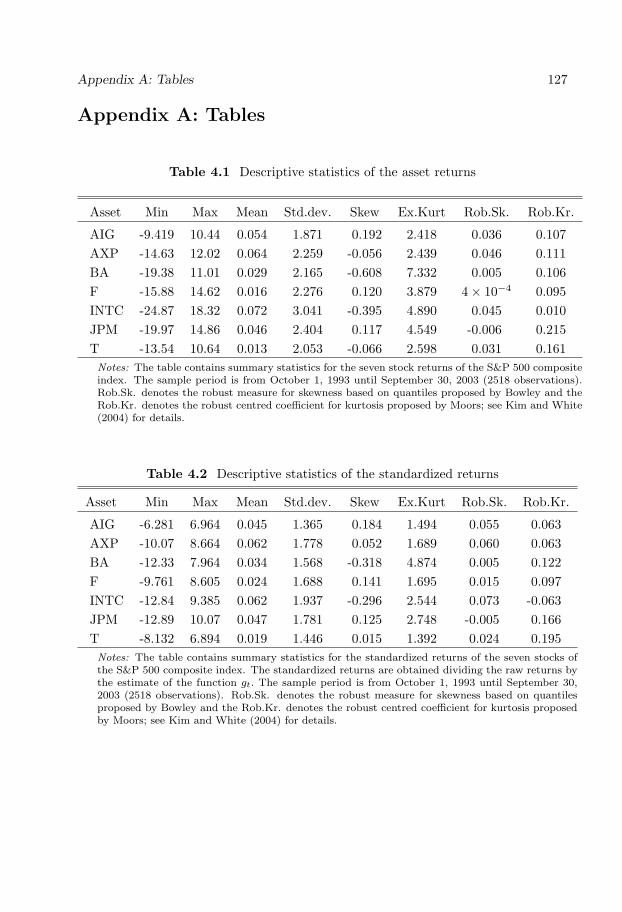
Appendix A: Tables 127
Appendix A: Tables
Table 4.1 Descriptive statistics of the asset returns
Asset Min Max Mean Std.dev. Skew Ex.Kurt Rob.Sk. Rob.Kr.
AIG -9.419 10.44 0.054 1.871 0.192 2.418 0.036 0.107AXP -14.63 12.02 0.064 2.259 -0.056 2.439 0.046 0.111BA -19.38 11.01 0.029 2.165 -0.608 7.332 0.005 0.106F -15.88 14.62 0.016 2.276 0.120 3.879 4× 10⁻⁴ 0.095INTC -24.87 18.32 0.072 3.041 -0.395 4.890 0.045 0.010JPM -19.97 14.86 0.046 2.404 0.117 4.549 -0.006 0.215T -13.54 10.64 0.013 2.053 -0.066 2.598 0.031 0.161Notes: The table contains summary statistics for the seven stock returns of the S&P 500 compositeindex. The sample period is from October 1, 1993 until September 30, 2003 (2518 observations).Rob.Sk. denotes the robust measure for skewness based on quantiles proposed by Bowley and theRob.Kr. denotes the robust centred coefficient for kurtosis proposed by Moors; see Kim and White(2004) for details.
Table 4.2 Descriptive statistics of the standardized returns
Asset Min Max Mean Std.dev. Skew Ex.Kurt Rob.Sk. Rob.Kr.
AIG -6.281 6.964 0.045 1.365 0.184 1.494 0.055 0.063AXP -10.07 8.664 0.062 1.778 0.052 1.689 0.060 0.063BA -12.33 7.964 0.034 1.568 -0.318 4.874 0.005 0.122F -9.761 8.605 0.024 1.688 0.141 1.695 0.015 0.097INTC -12.84 9.385 0.062 1.937 -0.296 2.544 0.073 -0.063JPM -12.89 10.07 0.047 1.781 0.125 2.748 -0.005 0.166T -8.132 6.894 0.019 1.446 0.015 1.392 0.024 0.195Notes: The table contains summary statistics for the standardized returns of the seven stocks ofthe S&P 500 composite index. The standardized returns are obtained dividing the raw returns bythe estimate of the function gt. The sample period is from October 1, 1993 until September 30,2003 (2518 observations). Rob.Sk. denotes the robust measure for skewness based on quantilesproposed by Bowley and the Rob.Kr. denotes the robust centred coefficient for kurtosis proposedby Moors; see Kim and White (2004) for details.

128 Chapter 4
Table 4.3 Sequence of tests of constant unconditional variance against a time-varyingGARCH model with multiplicative structure
Transitions in thealternative model H0 H03 H02 H01
Single transitionAIG 1× 10⁻²¹ 0.0120 0.0044 1× 10⁻²⁰
AXP 6× 10⁻²⁵ 2× 10⁻¹⁰ 1× 10⁻⁵ 3× 10⁻¹⁴
BA 3× 10⁻¹⁰ 0.0019 0.0015 1× 10⁻⁷
F 1× 10⁻²⁰ 0.0359 0.0491 8× 10⁻²¹
INTC 2× 10⁻²⁰ 2× 10⁻⁸ 0.0627 6× 10⁻¹⁵
JPM 1× 10⁻¹⁹ 5× 10⁻⁵ 0.0513 2× 10⁻¹⁷
T 2× 10⁻²⁵ 8× 10⁻⁷ 0.3812 3× 10⁻²²
Double transitionAIG 0.1127 0.0418 0.5284 0.2297AXP 4× 10⁻⁴ 0.2735 0.0073 0.0016BA 0.2419 0.2362 0.3391 0.1712F 0.0084 0.3381 0.3607 0.0016INTC 3× 10⁻⁵ 0.8513 1× 10⁻⁵ 0.0277JPM 0.1421 0.9199 0.0352 0.3175T 0.0939 0.0174 0.7878 0.4116
Triple transitionAIG − − − −AXP 0.2405 0.1536 0.3026 0.2932BA − − − −F 0.3205 0.1264 0.8555 0.2869INTC 0.0433 0.2563 0.0210 0.2170JPM − − − −T − − − −
Notes: The entries are the p-values of the LM-type tests of constant unconditional varianceapplied to the seven stock returns of the S&P 500 composite index. The appropriate orderk in (4.9) is chosen from the short sequence of hypothesis as follows: If the smallest p-valueof the test corresponds to H02, then choose k = 2. If either H01 or H03 are rejected morestrongly than H02, then select either k = 1 or k = 3. See Amado and Terasvirta (2008) forfurther details.

Appendix A: Tables 129
Table 4.4 Estimation results for the univariate TV-GJR-GARCH models
Asset δ1 γ1 c11 δ2 γ2 c21 c22 r
gt component
AIG 1.2550(0.0803)
100(−)
0.3709(0.0028)
— — — — 1
AXP 1.4280(0.1218)
100(−)
0.4815(0.0025)
-0.8940(0.1568)
100(−)
0.8022(0.0032)
— 2
BA 1.4708(0.0902)
100(−)
0.4041(0.0027)
— — — — 1
F 1.0413(0.0979)
100(−)
0.4426(0.0030)
0.8489(0.2003)
100(−)
0.7872(0.0038)
— 2
INTC 0.2720(0.0310)
100(−)
0.1650(0.0020)
-0.6862(0.0209)
100(−)
0.6180(0.0106)
0.9240(0.0118)
2
JPM 1.3984(0.0938)
100(−)
0.4814(0.0026)
— — — — 1
T 1.7708(0.1048)
100(−)
0.4442(0.0023)
— — — — 1
Notes: The table contains the parameter estimates of the git component from theTV-GJR-GARCH(1,1) model for the seven stocks of the S&P 500 composite index,over the period October 1, 1993 - September 30, 2003. The estimated model has theform git = 1 +
∑rl=1 δilGil(t/T ; γil, cil), where Gil(t/T ; γil, cil) is defined in (4.9) for
all i. The numbers in parentheses are the standard errors.
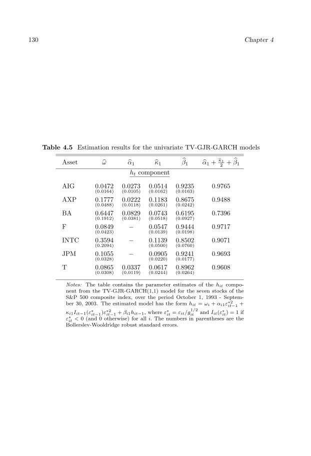
130 Chapter 4
Table 4.5 Estimation results for the univariate TV-GJR-GARCH models
Asset ω α1 κ1 β1 α1 + κ12 + β1
ht component
AIG 0.0472(0.0164)
0.0273(0.0105)
0.0514(0.0162)
0.9235(0.0163)
0.9765
AXP 0.1777(0.0488)
0.0222(0.0118)
0.1183(0.0261)
0.8675(0.0242)
0.9488
BA 0.6447(0.1912)
0.0829(0.0381)
0.0743(0.0518)
0.6195(0.0927)
0.7396
F 0.0849(0.0423)
− 0.0547(0.0139)
0.9444(0.0198)
0.9717
INTC 0.3594(0.2094)
− 0.1139(0.0500)
0.8502(0.0760)
0.9071
JPM 0.1055(0.0328)
− 0.0905(0.0220)
0.9241(0.0177)
0.9693
T 0.0865(0.0308)
0.0337(0.0119)
0.0617(0.0244)
0.8962(0.0264)
0.9608
Notes: The table contains the parameter estimates of the hit compo-nent from the TV-GJR-GARCH(1,1) model for the seven stocks of theS&P 500 composite index, over the period October 1, 1993 - Septem-ber 30, 2003. The estimated model has the form hit = ωi + αi1ε
∗2it−1 +
κi1Iit−1(ε∗it−1)ε∗2it−1 + βi1hit−1, where ε∗it = εit/g1/2it and Iit(ε
∗it) = 1 if
ε∗it < 0 (and 0 otherwise) for all i. The numbers in parentheses are theBollerslev-Wooldridge robust standard errors.
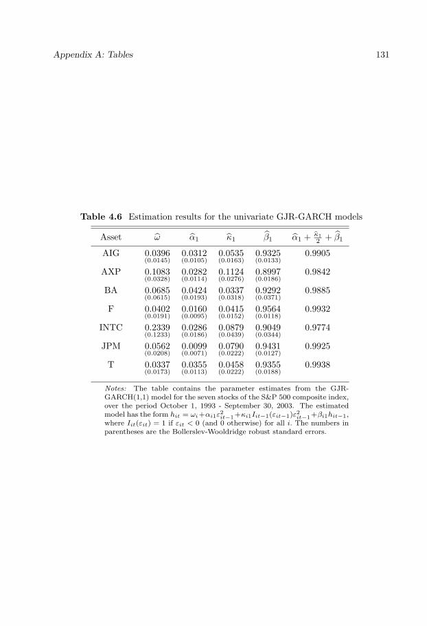
Appendix A: Tables 131
Table 4.6 Estimation results for the univariate GJR-GARCH models
Asset ω α1 κ1 β1 α1 + κ12 + β1
AIG 0.0396(0.0145)
0.0312(0.0105)
0.0535(0.0163)
0.9325(0.0133)
0.9905
AXP 0.1083(0.0328)
0.0282(0.0114)
0.1124(0.0276)
0.8997(0.0186)
0.9842
BA 0.0685(0.0615)
0.0424(0.0193)
0.0337(0.0318)
0.9292(0.0371)
0.9885
F 0.0402(0.0191)
0.0160(0.0095)
0.0415(0.0152)
0.9564(0.0118)
0.9932
INTC 0.2339(0.1233)
0.0286(0.0186)
0.0879(0.0439)
0.9049(0.0344)
0.9774
JPM 0.0562(0.0208)
0.0099(0.0071)
0.0790(0.0222)
0.9431(0.0127)
0.9925
T 0.0337(0.0173)
0.0355(0.0113)
0.0458(0.0222)
0.9355(0.0188)
0.9938
Notes: The table contains the parameter estimates from the GJR-GARCH(1,1) model for the seven stocks of the S&P 500 composite index,over the period October 1, 1993 - September 30, 2003. The estimatedmodel has the form hit = ωi+αi1ε
2it−1+κi1Iit−1(εit−1)ε2it−1+βi1hit−1,
where Iit(εit) = 1 if εit < 0 (and 0 otherwise) for all i. The numbers inparentheses are the Bollerslev-Wooldridge robust standard errors.

132 Chapter 4
Table 4.7 Misspecification tests for the GJR-GARCH models
(a) LM test of no ARCH in the standardized residuals
Return AIG AXP BA F INTC JPM Tr = 1 0.133 0.180 0.243 0.018 0.786 0.435 0.215r = 5 0.568 0.670 0.314 0.170 0.822 0.776 0.700r = 10 0.253 0.727 0.362 0.302 0.812 0.902 0.766
(b) LM test of GJR-GARCH(1,1) vs. GJR-GARCH(1,2) model
Return AIG AXP BA F INTC JPM T0.404 0.773 0.001 0.374 0.320 0.308 0.965
(c) LM test of GJR-GARCH(1,1) vs. GJR-GARCH(2,1) model
Return AIG AXP BA F INTC JPM T0.490 0.607 0.007 0.026 0.049 0.272 0.482
(d) LM type test of no additional transition in the function gt
Return AIG AXP BA F INTC JPM T0.003 2× 10⁻⁴ 0.008 0.001 10× 10−5 0.016 0.003
(e) LM type test of no ST-GJR-GARCH model of order 1
Return AIG AXP BA F INTC JPM T0.795 0.685 0.403 0.007 0.286 0.165 0.626
Notes: The entries are the p-values of the LM-type misspecification tests in Amadoand Terasvirta (2008). The diagnostic tests are the following: (a) test of no ARCH-in-GARCH against remaining ARCH of order r in the standardized residuals; (b)test of a GJR-GARCH(1,1) model against a GJR-GARCH(1,2) model; (c) testof a GJR-GARCH(1,1) model against a GJR-GARCH(2,1) model; (d) test of noadditional transition against another transition function in gt; (e) test of no remain-ing nonlinearity against a Smooth Transition GJR-GARCH (ST-GJR-GARCH) oforder k = 1.

Appendix A: Tables 133
Table 4.8 Misspecification tests for the TV-GJR-GARCH models
(a) LM test of no ARCH in the standardized residuals
Return AIG AXP BA F INTC JPM Tr = 1 0.112 0.077 0.907 0.104 0.993 0.429 0.390r = 5 0.641 0.429 0.956 0.360 0.881 0.871 0.759r = 10 0.392 0.570 0.725 0.340 0.557 0.960 0.749
(b) LM test of GJR-GARCH(1,1) vs. GJR-GARCH(1,2) model
Return AIG AXP BA F INTC JPM T0.579 0.700 0.208 0.411 0.191 0.487 0.819
(c) LM test of GJR-GARCH(1,1) vs. GJR-GARCH(2,1) model
Return AIG AXP BA F INTC JPM T0.878 0.943 0.741 0.419 0.071 0.702 0.557
(d) LM type test of no additional transition in the function gt
Return AIG AXP BA F INTC JPM T0.660 0.085 0.128 0.718 0.855 0.587 0.453
(e) LM type test of no ST-GJR-GARCH model of order 1
Return AIG AXP BA F INTC JPM T0.630 0.265 0.123 0.015 0.442 0.170 0.846
Notes: The entries are the p-values of the LM-type misspecification testsin Amado and Terasvirta (2008). The diagnostic tests are the following:(a) test of no ARCH-in-GARCH against remaining ARCH of order r inthe standardized residuals; (b) test of a GJR-GARCH(1,1) model againsta GJR-GARCH(1,2) model; (c) test of a GJR-GARCH(1,1) model againsta GJR-GARCH(2,1) model; (d) test of no additional transition against an-other transition function in gt; (e) test of no remaining nonlinearity againsta Smooth Transition GJR-GARCH (ST-GJR-GARCH) of order k = 1.

134 Chapter 4
Table 4.9 Log-likelihood values from the bivariate normal density for the CC-GJR-GARCH estimated models
Pairs of CCC DCC TVCCAssets GJR TV-GJR GJR TV-GJR GJR TV-GJR
AIG−AXP −9965.1 −8834.7 −9937.2 −8798.7 −9934.4 −8801.2
AIG−BA −10176.6 −8805.8 −10166.8 −8795.9 −10162.2 −8789.6
AIG−F −10256.1 −8999.0 −10250.2 −8989.9 −10249.6 −8991.8
AIG−INTC −11007.0 −9366.1 −10991.0 −9348.7 −10991.7 −9345.1
AIG−JPM −10084.6 −8851.0 −10050.6 −8813.2 −10058.6 −8821.3
AIG−T −9947.4 −8556.8 −9941.6 −8552.4 −9938.6 −8547.9
AXP−BA −10658.2 −9461.8 −10623.3 −9430.5 −10623.5 −9429.8
AXP−F −10712.7 −9624.7 −10697.6 −9606.7 −10704.2 −9613.4
AXP−INTC −11459.6 −9988.8 −11432.9 −9961.0 −11428.2 −9953.9
AXP−JPM −10445.9 −9381.6 −10388.2 −9315.7 −10409.4 −9334.6
AXP−T −10466.0 −9248.4 −10454.1 −9233.2 −10447.2 −9228.3
BA−F −10741.8 −9422.1 −10734.3 −9415.0 −10726.1 −9405.5
BA−INTC −11481.5 −9780.2 −11463.6 −9761.9 −11464.2 −9756.7
BA−JPM −10769.5 −9470.4 −10752.4 −9455.9 −10750.1 −9446.8
BA−T −10485.0 −9037.9 −10475.3 −9029.6 −10471.0 −9022.6
F−INTC −11537.5 −9937.9 −11522.4 −9924.7 −11526.9 −9924.5
F−JPM −10786.9 −9593.6 −10768.7 −9576.5 −10771.5 −9572.8
F−T −10578.2 −9237.6 −10575.4 −9233.6 −10569.8 −9226.9
INTC−JPM −11540.4 −9966.7 −11527.4 −9951.2 −11522.7 −9941.8
INTC−T −11314.7 −9594.2 −11306.7 −9585.9 −11298.6 −9575.5
JPM−T −10569.5 −9247.9 −10555.7 −9233.4 −10546.5 −9224.3
Notes: The table contains the log-likelihood values for each of the bivariate CC-GJR-GARCHmodel. The conditional variances are modelled as GJR-GARCH(1,1). The GJR column indicatesthat the unconditional variances are time-invariant functions. The TV-GJR column indicates thatthe unconditional variances vary over time according to function (4.8). The maximized values forthe log-likelihood are shown in boldface.

Appendix A: Tables 135
Table 4.10 Estimation results for the bivariate TVCC-GJR-GARCH models
Pairs of assets ρ(1) ρ(2) γ c
AIG−AXP 0.4564(0.0338)
0.7394(0.0177)
500(−)
0.88(0.001)
AIG−BA 0.2193(0.0379)
0.4907(0.0454)
15.06(66.91)
0.85(0.09)
AIG−F 0.2647(0.0211)
0.4490(0.0604)
500(−)
0.88(0.001)
AIG−INTC 0.1992(0.0274)
0.5000(0.0667)
9.51(6.05)
0.85(0.06)
AIG−JPM 0.4422(0.0216)
0.6948(0.0244)
500(−)
0.86(0.000)
AIG−T 0.2906(0.0219)
0.4785(0.0397)
500(−)
0.85(0.001)
AXP−BA 0.1839(0.0272)
0.4954(0.0305)
139.98(114.18)
0.71(0.01)
AXP−F 0.2880(0.0223)
0.4436(0.0383)
500(−)
0.75(0.000)
AXP−INTC 0.2159(0.0257)
0.5137(0.0297)
44.61(52.01)
0.74(0.02)
AXP−JPM 0.3842(0.0330)
0.6241(0.0163)
500(−)
0.34(0.001)
AXP−T 0.2445(0.0230)
0.5377(0.0443)
32.43(21.82)
0.86(0.02)
BA−F 0.1789(0.0241)
0.4136(0.0419)
500(−)
0.78(0.002)
BA−INTC 0.1390(0.0273)
0.3820(0.0435)
500(−)
0.75(0.001)
BA−JPM 0.1984(0.0250)
0.4445(0.0426)
500(−)
0.74(0.001)
BA−T 0.1488(0.0214)
0.4217(0.0420)
33.64(15.056)
0.85(0.02)
F−INTC 0.2412(0.0226)
0.4743(0.0531)
500(−)
0.88(0.001)
F−JPM 0.3200(0.0331)
0.5888(0.0554)
15.56(64.01)
0.87(0.07)
F−T 0.1657(0.0237)
0.3572(0.0429)
500(−)
0.82(0.001)
INTC−JPM 0.2701(0.0265)
0.4962(0.0428)
500(−)
0.78(0.000)
INTC−T 0.1197(0.0235)
0.3834(0.0567)
159.43(105.88)
0.82(0.02)
JPM−T 0.2396(0.0222)
0.5473(0.0401)
500(−)
0.86(0.001)
Notes: The table contains the estimation results for eachof the bivariate TVCC-GJR-GARCH model. The condi-tional variances are modelled as GJR-GARCH(1,1) and theunconditional variances are time-invariant functions. Thenumbers in parentheses are the standard errors.

136 Chapter 4
Table 4.11 Estimation results for the bivariate TVCC-TVGJR-GARCH models
Pairs of assets ρ(1) ρ(2) γ cAIG−AXP 0.4504
(0.0175)0.7459(0.0224)
500(−)
0.88(0.001)
AIG−BA 0.2202(0.0235)
0.5390(0.1174)
6.54(4.09)
0.84(0.070)
AIG−F 0.1824(0.0341)
0.3303(0.0249)
53.85(51.68)
0.33(0.036)
AIG−INTC 0.1872(0.0240)
0.4554(0.0443)
144.64(37.18)
0.75(0.004)
AIG−JPM 0.4355(0.0218)
0.7052(0.0236)
109.72(52.88)
0.86(0.007)
AIG−T 0.2954(0.0211)
0.4786(0.0387)
500(−)
0.84(0.001)
AXP−BA 0.1910(0.0273)
0.5069(0.0373)
29.57(21.12)
0.73(0.025)
AXP−F 0.2033(0.0392)
0.3852(0.0256)
15.37(9.46)
0.37(0.053)
AXP−INTC 0.2137(0.0240)
0.5327(0.0306)
40.15(19.92)
0.74(0.011)
AXP−JPM 0.3705(0.0338)
0.6397(0.0173)
23.58(16.22)
0.36(0.033)
AXP−T 0.2414(0.0230)
0.5413(0.0626)
25.43(29.86)
0.85(0.032)
BA−F 0.1746(0.0230)
0.4172(0.0413)
500(−)
0.75(0.001)
BA−INTC 0.1366(0.0251)
0.4342(0.0436)
144.19(38.35)
0.76(0.005)
BA−JPM 0.1975(0.0241)
0.4753(0.0409)
500(−)
0.74(0.001)
BA−T 0.1554(0.0211)
0.7707(0.2668)
6.62(2.06)
0.94(0.043)
F−INTC 0.2258(0.0234)
0.4369(0.0373)
500(−)
0.76(0.001)
F−JPM 0.3040(0.0222)
0.7842(0.5354)
4.56(4.05)
0.91(0.174)
F−T 0.1623(0.0232)
0.3826(0.0452)
500(−)
0.82(0.001)
INTC−JPM 0.2537(0.0267)
0.5291(0.0468)
24.54(11.48)
0.74(0.019)
INTC−T 0.1183(0.0228)
0.4100(0.0559)
500(−)
0.82(0.004)
JPM−T 0.2410(0.0223)
0.5462(0.0377)
500(−)
0.84(0.001)
Notes: The table contains the estimation results for each of thebivariate TVCC-TVGJR-GARCH model. The conditional vari-ances are modelled as GJR-GARCH(1,1) and the unconditionalvariances vary over time according to function (4.8). The numbersin parentheses are the standard errors.

Appendix B: Figures 137
Appendix B: Figures
0 500 1000 1500 2000 2500−10
−5
0
5
10
(a) AIG returns
0 500 1000 1500 2000 2500
−14
−8
−2
4
10
(b) AXP returns
0 500 1000 1500 2000 2500
−18
−12
−6
0
6
12
(c) BA returns
0 500 1000 1500 2000 2500−15
−10
−5
0
5
10
15
(d) F returns
0 500 1000 1500 2000 2500−24
−16
−8
0
8
16
(e) INTC returns
0 500 1000 1500 2000 2500
−18
−12
−6
0
6
12
(f) JPM returns
0 500 1000 1500 2000 2500
−12
−6
0
6
12
(g) T returns
Figure 4.1 The seven stock returns of the S&P 500 composite index from October1, 1993 until September 30, 2003 (2518 observations).

138 Chapter 4
0 500 1000 1500 2000 2500
1.0
1.5
2.0
2.5
(a) AIG returns
0 500 1000 1500 2000 2500
1.0
1.5
2.0
2.5
(b) AXP returns
0 500 1000 1500 2000 2500
1.0
1.5
2.0
2.5
(c) BA returns
0 500 1000 1500 2000 2500
1.0
1.5
2.0
2.5
3.0
(d) F returns
0 500 1000 1500 2000 25000.25
0.50
0.75
1.00
1.25
(e) INTC returns
0 500 1000 1500 2000 2500
1.0
1.5
2.0
2.5
(f) JPM returns
0 500 1000 1500 2000 2500
1.0
1.5
2.0
2.5
3.0
(g) T returns
Figure 4.2 Estimated gt functions for the seven stock returns of the S&P 500composite index.

Appendix B: Figures 139
0 500 1000 1500 2000 25001
2
3
4
5
(a) AIG returns
0 500 1000 1500 2000 2500
2
3
4
5
6
7
(b) AXP returns
0 500 1000 1500 2000 2500
2
3
4
5
6
7
(c) BA returns
0 500 1000 1500 2000 2500
2
3
4
5
6
(d) F returns
0 500 1000 1500 2000 25002
4
6
8
10
(e) INTC returns
0 500 1000 1500 2000 2500
2
3
4
5
6
7
8
(f) JPM returns
0 500 1000 1500 2000 25001
2
3
4
5
6
(g) T returns
Figure 4.3 Estimated conditional standard deviations from the GJR(1,1) model forthe seven stock returns of the S&P 500 composite index.

140 Chapter 4
10 20 30 40 50 60 70 80 90 100
0.0
0.1
0.2
0.3
0.4
(a) AIG returns
10 20 30 40 50 60 70 80 90 100
0.0
0.1
0.2
0.3
0.4
(b) AXP returns
10 20 30 40 50 60 70 80 90 100
0.0
0.1
0.2
0.3
0.4
(c) BA returns
10 20 30 40 50 60 70 80 90 100
0.0
0.1
0.2
0.3
0.4
(d) F returns
10 20 30 40 50 60 70 80 90 100
0.0
0.1
0.2
0.3
0.4
(e) INTC returns
10 20 30 40 50 60 70 80 90 100
0.0
0.1
0.2
0.3
0.4
(f) JPM returns
10 20 30 40 50 60 70 80 90 100
0.0
0.1
0.2
0.3
0.4
0.5
(g) T returns
Figure 4.4 Sample autocorrelation functions of the absolute value for the seven stockreturns of the S&P 500 composite index. The horizontal lines are the corresponding95% confidence interval under the iid normality assumption.

Appendix B: Figures 141
0 500 1000 1500 2000 25001
2
3
4
5
(a) AIG returns
0 500 1000 1500 2000 2500
2
3
4
5
6
7
(b) AXP returns
0 500 1000 1500 2000 2500
2
3
4
5
6
7
(c) BA returns
0 500 1000 1500 2000 2500
2
3
4
5
6
(d) F returns
0 500 1000 1500 2000 2500
2
4
6
8
10
(e) INTC returns
0 500 1000 1500 2000 2500
2
3
4
5
6
7
8
(f) JPM returns
0 500 1000 1500 2000 25001
2
3
4
5
6
(g) T returns
Figure 4.5 Estimated conditional standard deviations from the GJR(1,1) model forthe standardized variable εt/g
1/2t for the seven stock returns of the S&P 500 composite
index.

142 Chapter 4
10 20 30 40 50 60 70 80 90 100
0.0
0.1
0.2
0.3
0.4
(a) AIG returns10 20 30 40 50 60 70 80 90 100
0.0
0.1
0.2
0.3
0.4
(b) AXP returns10 20 30 40 50 60 70 80 90 100
0.0
0.1
0.2
0.3
0.4
(c) BA returns
10 20 30 40 50 60 70 80 90 100
0.0
0.1
0.2
0.3
0.4
(d) F returns10 20 30 40 50 60 70 80 90 100
0.0
0.1
0.2
0.3
0.4
(e) INTC returns10 20 30 40 50 60 70 80 90 100
0.0
0.1
0.2
0.3
0.4
(f) JPM returns
10 20 30 40 50 60 70 80 90 100
0.0
0.1
0.2
0.3
0.4
(g) T returns
Figure 4.6 Sample autocorrelation functions of the absolute value of the standard-ized variable εt/g
1/2t for the seven stock returns of the S&P 500 composite index. The
horizontal lines are the corresponding 95% confidence interval under the iid normalityassumption.

Appendix B: Figures 143
050
010
0015
0020
0025
00
−0.14−0.050.040.13
(a)
AIG
-AX
P
050
010
0015
0020
0025
00
−0.05−0.020.010.04
(b)
AIG
-BA
050
010
0015
0020
0025
00
−0.08−0.030.020.07
(c)
AX
P-B
A
050
010
0015
0020
0025
00
−0.04−0.010.020.05
(d)
AIG
-F0
500
1000
1500
2000
2500
−0.08−0.020.040.10
(e)
AX
P-F
050
010
0015
0020
0025
00
−0.030.000.030.06
(f)
BA
-F
050
010
0015
0020
0025
00
−0.06−0.030.000.03
(g)
AIG
-IN
TC
050
010
0015
0020
0025
00
−0.08−0.030.020.07 (h)
AX
P-I
NT
C0
500
1000
1500
2000
2500
−0.06−0.020.020.06
(i)
BA
-IN
TC
050
010
0015
0020
0025
00
−0.07−0.030.010.05
(j)
F-I
NT
C
050
010
0015
0020
0025
00
−0.05−0.020.010.04
(k)
AIG
-JPM
050
010
0015
0020
0025
00
−0.08−0.030.020.07
(l)
AX
P-J
PM
050
010
0015
0020
0025
00
−0.08−0.020.040.10
(m)
BA
-JPM
050
010
0015
0020
0025
00
−0.04−0.010.020.05
(n)
F-J
PM
050
010
0015
0020
0025
00
−0.04−0.010.020.05
(o)
INT
C-J
PM
050
010
0015
0020
0025
00
−0.06−0.030.000.03
(p)
AIG
-T0
500
1000
1500
2000
2500
−0.03−0.010.010.03
(q)
AX
P-T
050
010
0015
0020
0025
00
−0.03−0.010.010.03
(r)
BA
-T0
500
1000
1500
2000
2500
−0.04−0.010.020.05
(s)
F-T
050
010
0015
0020
0025
00−0.03−0.010.010.03
(t)
INT
C-T
050
010
0015
0020
0025
00
−0.020.000.020.04
(u)
JPM
-T
Fig
ure
4.7
Diff
eren
cebe
twee
nth
ees
tim
ated
cond
itio
nalc
orre
lati
ons
obta
ined
from
the
biva
riat
eD
CC
-GJR
-GA
RC
Han
dth
ebi
vari
ate
DC
C-T
VG
JR-G
AR
CH
mod
els
for
the
asse
tre
turn
s.

144 Chapter 4
050
010
0015
0020
0025
000.
0
0.2
0.4
0.6
0.8
1.0
(a)
AIG
-AX
P
050
010
0015
0020
0025
000.
0
0.2
0.4
0.6
0.8
1.0
(b)
AIG
-BA
050
010
0015
0020
0025
000.
0
0.2
0.4
0.6
0.8
1.0
(c)
AX
P-B
A
050
010
0015
0020
0025
000.
0
0.2
0.4
0.6
0.8
1.0
(d)
AIG
-F0
500
1000
1500
2000
2500
0.0
0.2
0.4
0.6
0.8
1.0
(e)
AX
P-F
050
010
0015
0020
0025
000.
0
0.2
0.4
0.6
0.8
1.0
(f)
BA
-F
050
010
0015
0020
0025
000.
0
0.2
0.4
0.6
0.8
1.0
(g)
AIG
-IN
TC
050
010
0015
0020
0025
000.
0
0.2
0.4
0.6
0.8
1.0
(h)
AX
P-I
NT
C0
500
1000
1500
2000
2500
0.0
0.2
0.4
0.6
0.8
1.0
(i)
BA
-IN
TC
050
010
0015
0020
0025
000.
0
0.2
0.4
0.6
0.8
1.0
(j)
F-I
NT
C
050
010
0015
0020
0025
000.
0
0.2
0.4
0.6
0.8
1.0
(k)
AIG
-JPM
050
010
0015
0020
0025
000.
0
0.2
0.4
0.6
0.8
1.0
(l)
AX
P-J
PM
050
010
0015
0020
0025
000.
0
0.2
0.4
0.6
0.8
1.0
(m)
BA
-JPM
050
010
0015
0020
0025
000.
0
0.2
0.4
0.6
0.8
1.0
(n)
F-J
PM
050
010
0015
0020
0025
000.
0
0.2
0.4
0.6
0.8
1.0
(o)
INT
C-J
PM
050
010
0015
0020
0025
000.
0
0.2
0.4
0.6
0.8
1.0
(p)
AIG
-T0
500
1000
1500
2000
2500
0.0
0.2
0.4
0.6
0.8
1.0
(q)
AX
P-T
050
010
0015
0020
0025
000.
0
0.2
0.4
0.6
0.8
1.0
(r)
BA
-T0
500
1000
1500
2000
2500
0.0
0.2
0.4
0.6
0.8
1.0
(s)
F-T
050
010
0015
0020
0025
000.
0
0.2
0.4
0.6
0.8
1.0
(t)
INT
C-T
050
010
0015
0020
0025
000.
0
0.2
0.4
0.6
0.8
1.0
(u)
JPM
-T
Fig
ure
4.8
The
esti
mat
edco
ndit
iona
lcor
rela
tion
sob
tain
edfr
omth
ebi
vari
ate
TV
CC
-GJR
-GA
RC
H(s
olid
curv
e)an
dth
ebi
vari
ate
TV
CC
-TV
GJR
-GA
RC
H(d
otte
dcu
rve)
mod
els
for
the
asse
tre
turn
s.

Appendix B: Figures 145
050
010
0015
0020
0025
00
0.2
0.4
0.6
0.8
1.0
(a)
AIG
-AX
P
050
010
0015
0020
0025
00
0.0
0.2
0.4
0.6
0.8
1.0
(b)
AIG
-BA
050
010
0015
0020
0025
00
0.0
0.2
0.4
0.6
0.8
1.0
(c)
AX
P-B
A
050
010
0015
0020
0025
00
0.0
0.2
0.4
0.6
0.8
1.0
(d)
AIG
-F0
500
1000
1500
2000
2500
0.0
0.2
0.4
0.6
0.8
1.0
(e)
AX
P-F
050
010
0015
0020
0025
000.
0
0.2
0.4
0.6
0.8
1.0
(f)
BA
-F
050
010
0015
0020
0025
00
−0.
2
0.0
0.2
0.4
0.6
0.8
1.0
(g)
AIG
-IN
TC
050
010
0015
0020
0025
00
0.0
0.2
0.4
0.6
0.8
1.0
(h)
AX
P-I
NT
C0
500
1000
1500
2000
2500
−0.
2
0.0
0.2
0.4
0.6
0.8
1.0
(i)
BA
-IN
TC
050
010
0015
0020
0025
00
0.0
0.2
0.4
0.6
0.8
1.0
(j)
F-I
NT
C
050
010
0015
0020
0025
00
0.2
0.4
0.6
0.8
1.0
(k)
AIG
-JPM
050
010
0015
0020
0025
00
0.2
0.4
0.6
0.8
1.0
(l)
AX
P-J
PM
050
010
0015
0020
0025
00
0.0
0.2
0.4
0.6
0.8
1.0
(m)
BA
-JPM
050
010
0015
0020
0025
00
0.0
0.2
0.4
0.6
0.8
1.0
(n)
F-J
PM
050
010
0015
0020
0025
00
0.0
0.2
0.4
0.6
0.8
1.0
(o)
INT
C-J
PM
050
010
0015
0020
0025
00
0.0
0.2
0.4
0.6
0.8
1.0
(p)
AIG
-T0
500
1000
1500
2000
2500
0.0
0.2
0.4
0.6
0.8
1.0
(q)
AX
P-T
050
010
0015
0020
0025
00
0.0
0.2
0.4
0.6
0.8
1.0
(r)
BA
-T0
500
1000
1500
2000
2500
0.0
0.2
0.4
0.6
0.8
1.0
(s)
F-T
050
010
0015
0020
0025
00−
0.2
0.0
0.2
0.4
0.6
0.8
1.0
(t)
INT
C-T
050
010
0015
0020
0025
000.
0
0.2
0.4
0.6
0.8
1.0
(u)
JPM
-T
Fig
ure
4.9
Diff
eren
cebe
twee
nth
ees
tim
ated
rolli
ngco
rrel
atio
nco
effici
ents
for
pair
sof
the
raw
retu
rns
(gre
ydo
tted
curv
e)an
dpa
irs
ofth
est
anda
rdiz
edre
turn
s(b
lack
solid
curv
e).

146 Chapter 4C
ovar
ianc
e
AXPAIG
−2 −1 01
2
−2−1
01
2
1.3
1.4
1.5
(a) lower regime
Cov
aria
nce
AXPAIG
−2 −1 01
2
−2−1
01
2
1.2
1.3
1.4
1.5
(b) upper regime
Figure 4.10 Estimated estimated time-varying news impact surfaces for the covari-ance between the AXP and AIG returns under the CCC-TVGJR-GARCH model inthe (a) lower regime and in the (b) upper regime of volatility.
AXPAIG
Var
ianc
e of
AIG
−1.5−0.5
0.51.5
−1.5
−0.5
0.5
1.5
0.90
0.95
1.00
1.05
1.10
(a) lower regime
AXPAIG
Var
ianc
e of
AIG
−1.5−0.5
0.51.5
−1.5
−0.5
0.5
1.5
0.90
0.95
1.00
1.05
1.10
(b) upper regime
Figure 4.11 Estimated time-varying news impact surfaces for the conditional vari-ance of the AIG returns under the CCC-TVGJR-GARCH model in the (a) lowerregime and (b) upper regime of volatility.
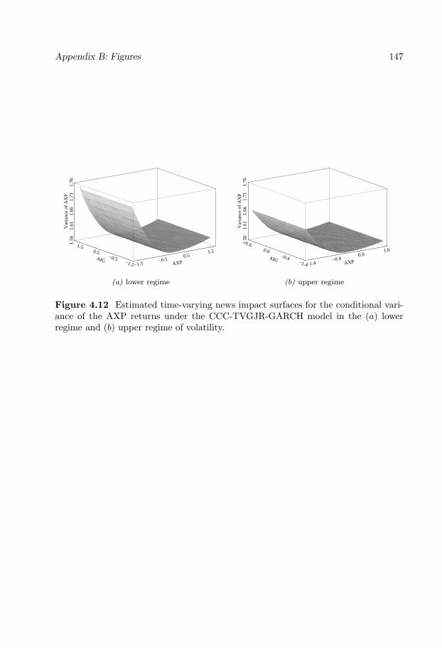
Appendix B: Figures 147
AXPAIG
Var
ianc
e of
AX
P
−1.5−0.5
0.51.5
−1.5
−0.5
0.5
1.5
1.56
1.61
1.66
1.71
1.76
(a) lower regime
AXPAIG
Var
ianc
e of
AX
P
−1.4−0.4
0.61.6
−1.4
−0.4
0.6
1.61.56
1.61
1.66
1.71
1.76
(b) upper regime
Figure 4.12 Estimated time-varying news impact surfaces for the conditional vari-ance of the AXP returns under the CCC-TVGJR-GARCH model in the (a) lowerregime and (b) upper regime of volatility.
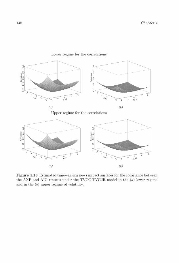
148 Chapter 4
Lower regime for the correlations
Cov
aria
nce
AXPAIG
−2 −1 01
2
−2−1
01
2
1.12
1.19
1.26
1.33
1.40
(a)
Cov
aria
nce
AXPAIG
−2 −1 01
2
−2−1
01
21.
121.
191.
261.
331.
40
(b)
Upper regime for the correlations
Cov
aria
nce
AXPAIG
−2 −1 01
2
−2−1
01
2
1.8
1.9
2.0
2.1
2.2
(a)
Cov
aria
nce
AXPAIG
−2 −1 01
2
−2−1
01
2
1.8
1.9
2.0
2.1
2.2
(b)
Figure 4.13 Estimated time-varying news impact surfaces for the covariance betweenthe AXP and AIG returns under the TVCC-TVGJR model in the (a) lower regimeand in the (b) upper regime of volatility.

Bibliography
Amado, C., and T. Terasvirta (2008): “Modelling Unconditional and ConditionalHeteroskedasticity with Smoothly Time-Varying Structure,” SSE/EFI Working Pa-per Series in Economics and Finance No. 691.
Bauwens, L., S. Laurent, and J. Rombouts (2006): “Multivariate GARCHModels: A Survey,” Journal of Applied Econometrics, 21, 79–109.
Berben, R.-P., and W. J. Jansen (2005): “Comovements in International EquityMarkets: A Sectorial View,” Journal of International Money and Finance, 24,832–857.
Bollerslev, T. (1990): “Modelling the Coherence in Short-Run Nominal ExchangeRates: A Multivariate Generalized ARCH Model,” The Review of Economic andStatistics, 72, 498–505.
Dahlhaus, R., and S. Subba Rao (2006): “Statistical Inference for Time-VaryingARCH Processes,” Annals of Statistics, 34, 1075–1114.
Diebold, F. X. (1986): “Comment on ”Modelling the Persistence of ConditionalVariance”, by R. Engle and T. Bollerslev,” Econometric Reviews, 5, 51–56.
Doornik, J. A. (2002): Object-Oriented Matrix Programming Using Ox. TimberlakeConsultants Press, see also www.nuff.ox.ac.uk/Users/Doornik, 3rd edn.
Engle, R. F. (2002): “Dynamic Conditional Correlation: A Simple Class of Multi-variate Generalized Autoregressive Conditional Heteroskedasticity Models,” Jour-nal of Business and Economic Statistics, 20, 339–350.
Engle, R. F., and J. Gonzalo Rangel (2008): “The Spline-GARCH Model forLow-Frequency Volatility and its Global Macroeconomic Causes,” Review of Fi-nancial Studies, 21, 1187–1222.
Engle, R. F., and V. Ng (1993): “Measuring and Testing the Impact of News onVolatility,” Journal of Finance, 48, 1749–1778.
Fan, Y., S. Pastorello, and E. Renault (2007): “Maximization by Parts inExtremum Estimation,” Unpublished paper.
149
150 Bibliography
Glosten, L. R., R. Jagannathan, and D. E. Runkle (1993): “On the RelationBetween the Expected Value and the Volatility of the Nominal Excess Return onStocks,” The Journal of Finance, 48, 1779–1801.
Hafner, C., and O. Linton (2008): “Efficient Estimation of a Multivariate Multi-plicative Model,” Unpublished paper.
Kim, T.-H., and H. White (2004): “On More Robust Estimation of Skewness andKurtosis,” Finance Research Letters, 1, 56–73.
Kroner, K. F., and V. K. Ng (1998): “Modeling Asymmetric Comovements ofAsset Returns,” Review of Financial Studies, 11, 817–844.
Lamoureux, C. G., and W. D. Lastrapes (1990): “Persistence in Variance, Struc-tural Change, and the GARCH Model,” Journal of Business & Economic Statistics,8, 225–234.
Ling, S., and M. McAleer (2003): “Asymptotic Theory for a New Vector ARMA-GARCH Model,” Econometric Theory, 19, 280–310.
Lutkepohl, H. (1996): Handbook of Matrices. John Wiley & Sons, Chichester.
Luukkonen, R., P. Saikkonen, and T. Terasvirta (1988): “Testing LinearityAgainst Smooth Transition Autoregressive Models,” Biometrika, 75, 491–499.
Mikosch, T., and C. Starica (2004): “Nonstationarities in Financial Time Series,the Long-Range Dependence, and the IGARCH Effects,” Review of Economics andStatistics, 86, 378–390.
Silvennoinen, A., and T. Terasvirta (2005): “Multivariate Autoregressive Con-ditional Heteroskedasticity with Smooth Transitions in Conditional Correlations,”SSE/EFI Working Paper Series in Economics and Finance No. 577.
(2007): “Modelling Multivariate Autoregressive Conditional Heteroskedas-ticity with the Double Smooth Transition Conditional Correlation GARCH Model,”SSE/EFI Working Paper Series in Economics and Finance No. 652.
(2008): “Multivariate GARCH Models,” in Handbook of Financial TimeSeries, ed. by T. G. Andersen, R. A. Davis, J.-P. Kreiss, and T. Mikosch. NewYork: Springer.
Tse, Y., and A. K. Tsui (2002): “A Multivariate GARCH Model with Time-VaryingCorrelations,” Journal of Business & Economic Statistics, 20, 351–362.

Chapter 5
A Smooth TransitionApproach to ModellingDiurnal Variation in Modelsof Autoregressive ConditionalDuration
151


153
A Smooth Transition Approach to Modelling Diurnal
Variation in Models of Autoregressive Conditional
Duration1
Abstract
This paper introduces a new approach for adjusting the diurnal variation in the tradedurations. The model considers that durations are multiplicatively decomposed intoa deterministic time-of-day and a stochastic component. The parametric structureof the diurnal component allows the duration process to change smoothly over thetime-of-day. In addition, a testing framework consisting of Lagrange multiplier testsis proposed for specifying the diurnal component. Our methodology is applied to theIBM transaction durations traded at the New York Stock Exchange.
1This paper is a joint work with Timo Terasvirta.Acknowledgements: This research has been supported by the Danish National Research Foun-
dation. The responsibility for any errors and shortcomings in this article remains ours.

154 Chapter 5
5.1 Introduction
The automated trading in financial markets and the development in computing powerhave made available intraday datasets containing recorded information of the trans-actions at the exchanges. Because transaction data arrive in irregularly spaced timeintervals, standard econometric methods are no longer applicable. The so-called high-frequency financial duration models were first introduced by Engle and Russell (1998)for tackling this inherent feature of the transaction data. These authors developedthe class of Autoregressive Conditional Duration (ACD) models, in which the timeelapsed between two market events (or duration) is the object of modelling. Theirmodel considers an autoregressive structure on the conditional expected durationswhose dynamics resembles the GARCH process for modelling the conditional vari-ances.
An important feature of financial durations is the evidence of a strong diurnalvariation over the trading day. Several studies have documented that trading activityis usually more intensive (shorter durations) near the opening and the closing ofthe market, and less intensive (longer durations) around lunchtime. Therefore, priorto using the ACD model any daily periodicity should be removed from the financialdurations. This observation has been first reported in Engle and Russell (1998) whoseprocedure is often used for taking into account the diurnal variation in the durations.Their approach consists of decomposing the durations into a deterministic component,that accounts for the diurnal variation, and a stochastic component for modelling thedurations dynamics. A common practice is to parameterize the diurnal componentaccording to a spline function; see Engle and Russell (1998) and Bauwens and Giot(2000). Some others methods have been considered in previous studies. McCullochand Tsay (2001) suggested a smooth quadratic function, whereas Zhang, Russell, andTsay (2001) have estimated the diurnal variation using the super smoother methodof Friedman (1984). As an alternative, Rodriguez-Poo, Veredas, and Espasa (2008)suggested a joint estimation of the deterministic and stochastic components in whichthe diurnal variation is estimated nonparametrically.
In this paper we follow Engle and Russell (1998) and let the durations be multi-plicatively decomposed into a deterministic and a stochastic component. We proposea new parameterization for the diurnal component in which the duration process isallowed to change smoothly over the time-of-day. In addition, we provide a testingframework for specifying the structure of the diurnal component by a sequence of La-grange multiplier tests. The empirical results suggest that the diurnal variation maynot always have the inverted U-shaped pattern for the trade durations as documentedin earlier studies. For this reason, one should proceed with care in the modelling ofthe time-of-day component.
The outline of the paper is as follows. In Section 5.2 we briefly review the ACDmodel. In Section 5.3 we present our method for removing the diurnal variation.Section 5.4 introduces the testing strategy for specifying the diurnal variation com-ponent. Section 5.5 contains the application for the IBM trade durations. Section 5.6concludes.

A Smooth Transition Approach to Modelling Diurnal Variation 155
5.2 The ACD framework
Let ti be the time (measured in seconds) at which the i−th trade occurs and the du-ration xi = ti− ti−1 be the time interval between two consecutive transactions occur-ring at times ti and ti−1. Let Fi−1 be the information set consisting of past durationsavailable at time ti−1. Following Engle and Russell (1998), the basic assumption ofthe ACD model is that the time dependence in the durations be captured by theirconditional expectation such that
xiE(xi|Fi−1)
≡ εi ∼ i.i.d. D($) (5.1)
where E(xi|Fi−1) = ψi(xi−1, . . . , x1;θψ) is the conditional mean duration on Fi−1,and D is a general distribution with positive support and parameter vector $. Inthe simplest ACD model, the durations are defined in terms of a multiplicative errorterm as
xi = ψiεi, (5.2)ψi = ψi(xi−1, . . . , x1;θψ), (5.3)
andεi ∼ i.i.d. exp(1) (5.4)
for i = 1, . . . , n. Equations (5.2)-(5.4) define the Exponential ACD model. The ex-pectation of the duration conditional on Fi−1 is specified as
ψi = ω +m∑j=1
αjxi−j +q∑j=1
βjψi−j . (5.5)
The condition 1−∑mj=1 αj−
∑qj=1 βj < 1 is necessary and sufficient for the existence
of E(xi). The parameter restrictions ω > 0, αj ≥ 0, j = 1, . . . ,m, and βj ≥ 0, j =1, . . . , q, are sufficient for the positivity of the conditional durations. For m = q = 1they are also necessary. Bauwens and Giot (2000) proposed a class of logaritmicACD models to ensure positiveness of the conditional durations without parametricconstraints. The autoregressive structure in equation (5.5) allows the model to ac-count for clustering of durations. Its dynamic structure resembles that of the GARCHmodel of Bollerslev (1986): it is a linear autoregressive process of past durations andconditional expectations. Consequently, many results and properties of the GARCHliterature can be adapted to the ACD context.
The distribution for the errors of the ACD model (5.1)-(5.3) is not limited to theexponential density as defined in (5.4). Other choices of distribution are possiblesuch as the Weibull, Burr, or generalized gamma distribution. Gourieroux, Monfort,and Trognon (1984) showed that the Quasi-Maximum Likelihood (QML) methodproduces consistent estimators of a correctly specified conditional mean model if andonly if the QML is based on a distribution belonging to the linear exponential family,and this holds even when the density is misspecified. For this reason, the QML

156 Chapter 5
estimators based on the exponential distribution will be consistent regardless the trueerror distribution, whereas the QML estimation based on densities not belongingto the linear exponential family such as the Weibull, Burr, or generalized gammadistributions will not produce consistent estimators. As an alternative, Drost andWerker (2004) showed that the QML estimators are consistent based on the standardgamma distribution. The score function of this log-likelihood, however, is proportionalto the one from the exponential density, and using either one of these two distributionsthus yields identical estimators.
5.3 Adjusting diurnal variation with smooth tran-sitions
It is well documented in the literature that trading market activity is subjected tosystematic variations over the time of the day. This is mainly because of the insti-tutional features of the exchanges. Trading activity is usually more intense at thebeginning and at the end of the day than it is around lunchtime. The high tradingactivity after the opening of the market occurs because traders want to adjust theirpositions to the information accumulated before the opening of the exchange. Thefrequency of transactions is also high near the closing of the market as traders wantto close their positions before the trading session ends. This leads to an invertedU-shaped pattern for the average intertrade durations over the trading day.
In order to account for this diurnal variation, the durations may be multiplica-tively decomposed into a deterministic and a stochastic component. The deterministiccomponent describes the intradaily pattern of the durations and the stochastic onerepresents the dynamics of the ACD-type model. The deterministic effect may beremoved from the data prior to estimating the ACD model. Engle and Russell (1998)suggested to ‘diurnally adjust’ the duration series by
xi = xi/φ(ti−1;θφ) (5.6)
in which xi is the adjusted duration and φ(ti−1;θφ) is the deterministic time-of-daycomponent. The expected duration equals
E(xi|Fi−1) = φ(ti−1;θφ)ψi(xi−1, . . . , x1;θψ) (5.7)
The component ψi is interpreted as the expected proportion above or below the normalduration level at that time of day.
The usual practice is to ‘diurnally adjust’ the duration series by estimating theaverage durations using a linear or a cubic spline function conditioned on the time-of-day and then remove this diurnal component from the original durations. Thediurnal pattern is estimated by averaging the durations over thirty minute intervals,and using a cubic spline over the course of the day to smooth the durations; seeBauwens and Giot (2000). The duration series is ‘diurnally adjusted’ by dividingthe original durations by the estimated diurnal component as in (5.6). This is doneseparately for each trading day as the time-of-day component may vary according to

A Smooth Transition Approach to Modelling Diurnal Variation 157
the day of the week. Alternatively, the parameter vectors θψ and θφ may be estimatedjointly by maximum likelihood. However, Engle and Russell (1998) pointed out thatthe two-step procedure and the joint estimation by ML yield almost the same resultsfor large samples.
Alternative ways of parameterizing the time-of-day effect exist. McCulloch andTsay (2001) have developed a linear regression method to remove the diurnal patternusing quadratic time functions and indicator variables. Furthermore, Rodriguez-Poo,Veredas, and Espasa (2008) suggested a semiparametric approach to the problemusing a simple transformation of the Nadaraya–Watson estimator to remove diurnalvariation from the process.
In this paper we propose to ‘diurnally adjust’ the durations by parameterizing thediurnal component as follows:
φ(ti−1;θφ) = δ0 +r∑l=1
δlGl(ti−1; γl, cl) (5.8)
where Gl(ti−1; γl, cl), l = 1, . . . , r, is a transition function bounded between zero andone. This implies that the duration process is assumed to change smoothly overthe time-of-day. In this context, the transition variable ti−1 is the intraday time(measured in seconds from the beginning of the trading day) which is for conveniencerescaled to run from zero to one. The transition function is the logistic function
Gl(ti−1; γl, cl) =
1 + exp
−γlk∏j=1
(ti−1 − clj)
−1
, l = 1, . . . , r, (5.9)
satisfying the identification restrictions γl > 0, cl1 ≤ cl2 ≤ ... ≤ clk. The slope param-eter γl controls the degree of smoothness of the transition function: the larger γl, thefaster the transition is between the extreme regimes. When γl −→∞, (5.9) becomes astep function, and the process switches instantaneously from one regime to the otherat ti−1 = clj . Typical choices for the transition function in practice are k = 1 andk = 2. When k = 2 the model can describe the aforementioned situation in whichtrading activity is higher in the beginning and then at the end of the session than itis in the middle of the day. Note that when δ1 = ... = δr = 0 in (5.8) there are nosystematic changes in the durations during the day. In this case, the durations tendto be uniformly exponentially distributed around their “normal” level. This specialcase is included in our model.
5.4 Specification tests for the diurnal component
In our framework, the structure of the diurnal component is determined by a sequenceof specification tests. These are based on statistical inference and they consist on twospecification tests. The first one tests the hypothesis of no diurnal variation againstdurations that change smoothly over the time-of-day. The other tests are for testingwhether yet another transition function is required in the definition of the diurnalcomponent.

158 Chapter 5
5.4.1 Testing for no diurnal variation
The test of no diurnal variation is an important tool for checking the presence ofsystematic changes over the time-of-day. The starting-point is that there is no sys-tematic change over the time-of-day while the alternative is that durations are varyingsmoothly during the day. In order to consider this testing problem let r = 1 in (5.8)and assume that the conditional duration process ψi = ω, i.e.
xi = ψiφiεi, εi ∼ i.i.d. exp(1) (5.10)ψiφi = ω{1 + δ1G1(ti−1; γ1, c1)} = ω + δ∗1G1(ti−1; γ1, c1). (5.11)
where ψi ≡ ψi(xi−1, . . . , x1;θψ), φi ≡ φ(ti−1;θφ) and δ∗1 = ωδ1. The null hypothesisof no diurnal variation is γ1 = 0 and the alternative γ1 > 0. The testing problem isnonstandard as δ∗1 and c1 are unidentified nuisance parameters when γ1 = 0. FollowingLuukkonen, Saikkonen, and Terasvirta (1988) we solve the identification problem byapproximating G1(ti−1; γ1, c1) with its third-order Taylor expansion around γ1 = 0 .After reparameterizing, we obtain
ψiφi = ω +3∑k=1
λktki−1 +R3(ti−1; γ1, c1) (5.12)
where λj = γ1δ∗j and R3(t/T ; γi1, ci1) is the remainder. Under H0, R3(ti−1; γ1, c1) ≡
0, so the asymptotic theory of the LM test statistic is not affected by this approxi-mation. The null hypothesis of no diurnal variation becomes H
′
0 : λ1 = λ2 = λ3 = 0.This hypothesis can be tested by an LM test as follows:
1. Estimate the conditional duration process under the assumption that ψi = ω,and compute ui = xi/ω − 1, i = 1, . . . , n, and SSR0 =
∑ni=1 u
2i .
2. Regress ui on x′1i = ω−1 and x′2i = (ti−1, t2i−1, t
3i−1)′, i = 1, . . . , n, and compute
SSR1.
3. Then, under the null hypothesis and the assumption ψi = ω, the test statistic
LM = n(SSR0 − SSR1)/SSR0
has an asymptotic χ2 distribution with three degrees of freedom.
We shall call our LM test statistic LMk, where k indicates the order of the polyno-mial in the exponent of the transition function. The rejection of the null hypothesisraises the problem of choosing k. In order to select k, we carry out a short sequence ofnested tests following Terasvirta (1994) and Lin and Terasvirta (1994). This is doneas follows. If parameter constancy is rejected at the significance level α(1), test thefollowing sequence of hypotheses:
H03 : λ3 = 0,H02 : λ2 = 0 | λ3 = 0,H01 : λ1 = λ2 = λ3 = 0 | λ2 = λ3 = 0,

A Smooth Transition Approach to Modelling Diurnal Variation 159
in (5.12), by means of LM-type tests. If H0i is rejected most strongly, measured bythe p-value, of the three hypotheses, one selects k = i. Visual inspection of the seriesmay sometimes also be helpful choosing k and can be used in parallel with the tests.
5.4.2 Testing the hypothesis of no additional transitions
After estimating the diurnal component with a single transition the next step is toinvestigate the possibility of remaining diurnal variation in the durations. In order todo that, the previous test must be generalized to the case where we test r = 1 againstr ≥ 2 in (5.8). To derive the test, consider the model
xi = ψiφiεi, εi ∼ i.i.d. exp(1) (5.13)ψiφi = ω + δ∗1G1(ti−1; γ1, c1) + δ∗2G2(ti−1; γ2, c2). (5.14)
The hypothesis of no additional transition is γ2 = 0. Again, the parameters δ∗2 andc2 are only identified under the alternative. The identification problem is solved asbefore, using a Taylor series approximation of G2(ti−1; γ2, c2) around γ2 = 0. Afterrearranging terms we have
ψiφi = ω + δ∗1G1(ti−1; γ1, c1) +3∑k=1
θktki−1 +R∗3(ti−1; γ2, c2) (5.15)
Under the null, the remainder R∗3(ti−1; γ2, c2) ≡ 0, so it does not affect the asymptotictheory. The new null hypothesis becomes H
′
02 : θ1 = θ2 = θ3 = 0. The significancelevel is now reduced by a factor τ ∈ (0, 1) in order to favour parsimony: α(2) = τα(1).In the application, we set τ = 0.5. Assuming ψi = ω, this hypothesis can be testedusing an LM test as before with ui = xi/ψiφi − 1, x′1i = ψ−1
i (φi + ψi∂φi
∂δ ), ∂φi
∂δ =(∂φi
∂δ∗1, ∂φi
∂γ1, ∂φi
∂c′1)′, and x′2i = φ−1
i (ti−1, t2i−1, t
3i−1)′, i = 1, . . . , n.
5.5 An application to the IBM trade durations
5.5.1 Data
The time series in this application consist of intertrade durations between transactionsof IBM shares traded at the New York Stock Exchange (NYSE). The original serieswere extracted from the Trade and Quote (TAQ) database available from the NYSE,and the sample period covers the entire month of December 2002. Besides detailedinformation about volume, transaction prices, and bid and ask quotes at the time ofthe trade, the database contains a time stamp, measured in seconds after midnightand indicating the time when the transaction occurred.
Prior to using the data, we remove the irregular transactions using the correctionindicator attached to each trade. Trades that occur before 9:30 AM and after 4:00PM are also excluded. Because the market was partly closed on December 24th, thisday has been removed from the data set. Furthermore, the overnight durations areignored as the trades are treated consecutively from day to day. This leaves us with

160 Chapter 5
0 10 20 30 40 50 60 70 8040
50
60
70
(a) Transactions: 5-min time intervals
0 10 20 30 40 50 60 70 80
5
6
7
8
(b) Durations: 5-min time intervals
Figure 5.1 Plots of the IBM transactions data in December 2002: (a) averagenumber of transactions in 5-minute time intervals; (b) average durations in 5-minutetime intervals.
20 trading days with a total of 82011 transactions at 76823 unique times. Multipletransactions within a second are considered as a single trade. Thus the minimum timebetween events is one second, whereas the maximum observed duration turns out tobe 142 seconds or 2 minutes and 22 seconds. The average duration between sucessiveevents is 6.09 seconds with a standard deviation of 6.22 seconds. Moreover, there isstrong autocorrelation in the durations as the Ljung-Box statistic of serial correlationup to the 15th order equals Q(15) = 1244 with p-value = 7 × 10−256. For modellingsuch dependence, we follow Engle and Russell (1998) and use the linear ACD model.At this stage, where the focus is on modelling the diurnal variation, we consider thesimplest version of the model. A better alternative such as a nonlinear ACD-typemodel would probably be needed to adequately capture the dynamic behaviour ofthe durations. Evidence of nonlinearity in the durations has been reported in Zhang,Russell, and Tsay (2001) and Meitz and Terasvirta (2006), among others.
Figure 5.1(a) displays the average number of transactions within 5-minute timeintervals over the 20 trading days. Each trading day contains 78 intervals. Theplot exhibits a U-shaped pattern indicating active trading at the opening and theclosing of the market and slower pace around the lunch hour. The average intradaydurations in 5-minute time intervals plotted in Figure 5.1(b) reinforces this feature.The durations are usually shorter at the beginning and the end of the trading day,and longer around midday, which yields an inverted U-shaped in the durations. Asthe intraday variation is repeated systematically for every trading day, the ACF ofthe number of transactions in 5-minute intervals is characterized by the periodicityshown in Figure 5.2.
Our analysis differs from the usual practice in the sense that we consider everyweek in the sample separately. This way we can accommodate possible calendar effectsover the time-of-week. However, a formal test is needed for testing the hypothesisof no systematic pattern over the days of the week. In case of rejection, the day-of-the week effect should be explicitly incorporated in the model. This problem is,
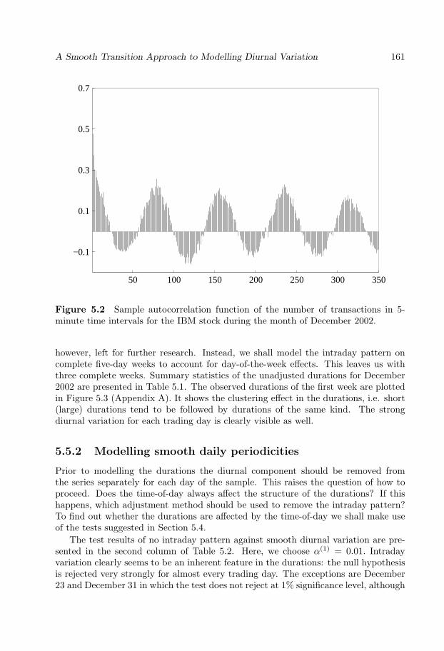
A Smooth Transition Approach to Modelling Diurnal Variation 161
50 100 150 200 250 300 350
−0.1
0.1
0.3
0.5
0.7
Figure 5.2 Sample autocorrelation function of the number of transactions in 5-minute time intervals for the IBM stock during the month of December 2002.
however, left for further research. Instead, we shall model the intraday pattern oncomplete five-day weeks to account for day-of-the-week effects. This leaves us withthree complete weeks. Summary statistics of the unadjusted durations for December2002 are presented in Table 5.1. The observed durations of the first week are plottedin Figure 5.3 (Appendix A). It shows the clustering effect in the durations, i.e. short(large) durations tend to be followed by durations of the same kind. The strongdiurnal variation for each trading day is clearly visible as well.
5.5.2 Modelling smooth daily periodicities
Prior to modelling the durations the diurnal component should be removed fromthe series separately for each day of the sample. This raises the question of how toproceed. Does the time-of-day always affect the structure of the durations? If thishappens, which adjustment method should be used to remove the intraday pattern?To find out whether the durations are affected by the time-of-day we shall make useof the tests suggested in Section 5.4.
The test results of no intraday pattern against smooth diurnal variation are pre-sented in the second column of Table 5.2. Here, we choose α(1) = 0.01. Intradayvariation clearly seems to be an inherent feature in the durations: the null hypothesisis rejected very strongly for almost every trading day. The exceptions are December23 and December 31 in which the test does not reject at 1% significance level, although

162 Chapter 5
Table 5.1 Summary statistics of the IBM durations
Durations Min Max Mean S.D. Skew. Ex.Kurt.
Week 1(02/12/02 - 06/12/02): T=20811
Raw 1 142 5.618 5.554 3.631 33.26Adjusted Spline 0.125 21.43 1.000 0.941 3.083 22.10Adjusted Smooth 0.130 19.01 0.933 0.895 3.069 19.90
Week 2(09/12/02 - 13/12/02): T=19248
Raw 1 81 6.074 6.101 2.893 13.71Adjusted Spline 0.113 13.19 1.000 0.966 2.768 13.01Adjusted Smooth 0.116 12.10 0.967 0.949 2.778 12.56
Week 3(16/12/02 - 20/12/02): T=18818
Raw 1 82 6.215 6.220 2.701 11.64Adjusted Spline 0.0951 12.18 0.999 0.961 2.533 10.07Adjusted Smooth 0.1226 13.66 0.956 0.949 2.698 11.97
Notes: Summary statistics for transaction duration data in seconds for the IBMstock traded at NYSE in December 2002.
the p-values still remain below the 5% level. This is explained by the irregular tradingactivity of these days due to their proximity to the Christmas Eve and the New Year’sDay. Note, however, that the test based on the first-order Taylor approximation doesreject the null hypothesis (it is H01) at the 1% level.
The tests of the last three columns correspond to a sequence of nested tests basedon (5.12) for choosing k in (5.9). In this context, k is related with the shape of diurnalpattern. As mentioned aboved, if H0i is rejected most strongly, measured by the p-value, of the three hypotheses, one selects k = i. The table shows k = 2 for sixteenout of nineteen days, whereas for the remaining days k = 1 is the appropriate choice.As already mentioned, the test of H01 is the test of no diurnal variation based on thefirst-order Taylor approximation. It has power against the single logistic transitionk = 1. Because the diurnal variation typically has an inverted U-shape, we fit thediurnal component φi with a single transition and then test for another transition.The resulting p-values are presented in Table 5.3. The hypothesis of one transitionagainst another transition in the diurnal component is still rejected at α(2) = 0.005for one trading day, but the rejection is much weaker than before. Consequently, thefunction φi with two transitions is chosen as the diurnal component for December16th.
For comparison, tests for October 2002 are also reported in Table 5.4 (AppendixB). Two outcomes deserve particular attention. First, the null hypothesis of no diurnal

A Smooth Transition Approach to Modelling Diurnal Variation 163
Table 5.2 p-values of the LM tests of no diurnal variation (December 2002)
Day H0 H03 H02 H01
02/12/2002 3× 10⁻¹⁵ 0.0169 3× 10⁻¹³ 5× 10⁻⁴
03/12/2002 9× 10⁻¹³ 0.2428 8× 10⁻¹³ 0.009704/12/2002 6× 10⁻¹⁵ 0.1887 2× 10⁻⁷ 2× 10⁻¹⁰
05/12/2002 6× 10⁻²² 0.3468 1× 10⁻¹⁷ 1× 10⁻⁷
06/12/2002 4× 10⁻⁷ 0.1053 9× 10⁻⁵ 1× 10⁻⁴
09/12/2002 1× 10⁻¹¹ 0.0927 1× 10⁻¹² 0.491310/12/2002 3× 10⁻²⁰ 0.9704 1× 10⁻²¹ 0.100511/12/2002 1× 10⁻¹¹ 7× 10⁻⁴ 2× 10⁻⁹ 0.009512/12/2002 3× 10⁻¹¹ 0.0071 2× 10⁻¹¹ 0.810813/12/2002 6× 10⁻⁵ 0.1327 9× 10⁻⁶ 0.592416/12/2002 3× 10⁻¹⁰ 1× 10⁻⁴ 0.0021 1× 10⁻⁶
17/12/2002 1× 10⁻²⁰ 2× 10⁻⁴ 4× 10⁻¹⁹ 0.178218/12/2002 5× 10⁻¹⁵ 0.7886 1× 10⁻¹² 1× 10⁻⁵
19/12/2002 1× 10⁻¹⁵ 0.0038 4× 10⁻¹³ 1× 10⁻⁴
20/12/2002 1× 10⁻¹⁷ 0.1157 4× 10⁻¹⁸ 0.034023/12/2002 0.0164 0.0666 0.0086 0.962726/12/2002 4× 10⁻⁸ 0.6262 5× 10⁻⁹ 0.106927/12/2002 2× 10⁻¹³ 0.2733 1× 10⁻⁹ 1× 10⁻⁶
31/12/2002 0.0360 0.5900 0.4609 0.0055
Notes: The table contains p-values of the LM tests of no diurnal variation againstsmoothly time-varying diurnal pattern in the durations for December 2002. The p-values shown in boldface indicate the lowest rejection rate.
pattern is not rejected for seven out of 23 trading days. The intraday pattern is thusconsiderably less conspicuous in October than in December, which suggests that thedurations may also vary systematically over the year besides the time of day. Second,when the null hypothesis is rejected, the tests support the usual inverted U-shape ofdiurnal variation only in four out of fifteen days. This suggests the diurnal patternmay not always have the shape proposed earlier: short durations early and late in theday and lower activity in the middle. For this reason, one should proceed with carewhen specifying the diurnal component. The estimation of the ACD model should bepreceded by a specification search to determine the diurnal variation.
For the empirical analysis, durations are ‘diurnally adjusted’ using two differentestimators for the diurnal component. The first estimator is cubic spline of Engle andRussell (1998), and the second one our smooth transition component. The adjusteddurations are obtained by dividing the raw durations by one of these deterministic

164 Chapter 5
Table 5.3 p-values of the LM tests of a single transition against a double transitionin the diurnal component
Day H0 H03 H02 H01
04/12/2002 0.0161 0.2310 0.0272 0.045516/12/2002 9× 10⁻⁵ 0.0476 0.0282 4× 10⁻⁴
31/12/2002 0.0967 0.4336 0.5983 0.0197Notes: The table contains p-values of the LM tests of no diurnal variationagainst smoothly time-varying diurnal pattern in the durations for Decem-ber 2002. The p-values shown in boldface indicate the lowest rejectionrate.
diurnal factors. The diurnal components estimated by cubic splines for each day of thesecond week of December are shown in Figure 5.4 whereas the ones estimated usingthe smooth transition approach can be found in Figure 5.5. The durations changesystematically through the day, and the pattern of trading activity accords to whathas been reported in earlier studies. Durations tend to be shorter at the beginningand at the end of the day and longer around lunch time. Some summary statistics ofthe adjusted durations can be found in Table 5.1.
Table 5.5 presents the estimation results for the two parameterizations of φi. Theparameter estimates are significant in the three weeks. The smooth diurnal compo-nent has a larger value of α1 + β1 than the cubic spline method. Similar results wereobtained by Rodriguez-Poo, Veredas, and Espasa (2008) who employed a semipara-metric model for the diurnal factor. Furthermore, the results indicate that the smoothtransition parameterization attains higher likelihood values, and therefore seems tofit durations better than the cubic spline approach.
5.6 Conclusions
In this paper we have introduced the smooth transition method for parameterizingthe diurnal variation in the intertrade durations. This is done by multiplicativelydecomposing durations into a deterministic and an stochastic component, in which thedurations are allowed to change smoothly over the time-of-day. A testing framework isalso provided for determining the structure of the diurnal component using a sequenceof specification tests.
Our modelling technique is illustrated with an application to IBM stock transac-tion data. The test results indicate that the diurnal variation may not always havethe documented inverted U-shaped pattern for the trade durations. In addition, theresults suggest that our method fits durations better than the cubic spline approach.
A possible extension of this framework is to jointly estimate the parametric condi-tional duration and diurnal variation components. This may be done by maximisationby parts as in Song, Fan, and Kalbfleisch (2005) in which the resulting estimator coin-cides with the ML estimator. This consideration is, however, left for future research.
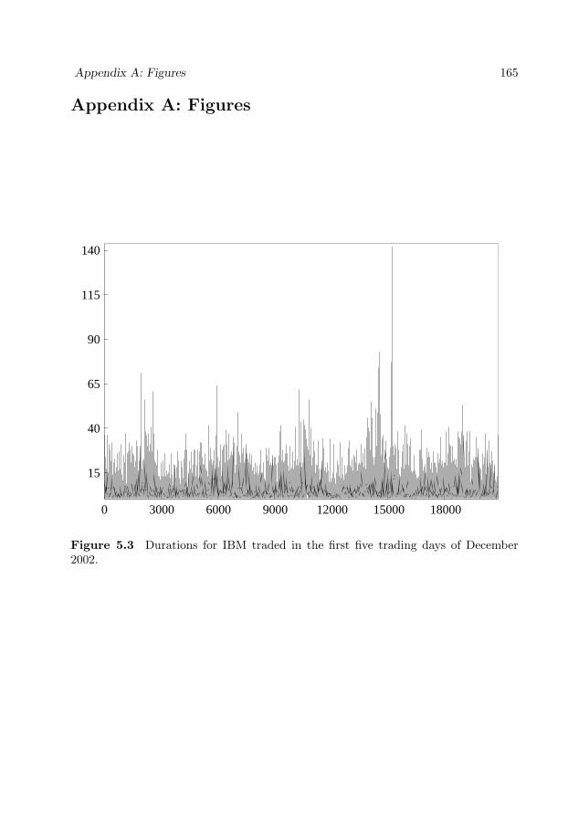
Appendix A: Figures 165
Appendix A: Figures
0 3000 6000 9000 12000 15000 18000
15
40
65
90
115
140
Figure 5.3 Durations for IBM traded in the first five trading days of December2002.

166 Appendix A: Figures
34000 37000 40000 43000 46000 49000 52000 55000 58000
5
6
7
8
(a) Monday
34000 37000 40000 43000 46000 49000 52000 55000 58000
5
6
7
8
(b) Tuesday
34000 37000 40000 43000 46000 49000 52000 55000 58000
4
5
6
7
8
9
(c) Wednesday
34000 37000 40000 43000 46000 49000 52000 55000 58000
4
5
6
7
8
(d) Thursday
34000 37000 40000 43000 46000 49000 52000 55000 58000
4
5
6
7
8
(e) Friday
Figure 5.4 Estimated diurnal variation using the cubic spline for the trade durationsof IBM in the second week of December 2002. The scale of the x-axis is time measuredin seconds after midnight.

Appendix A: Figures 167
34000 37000 40000 43000 46000 49000 52000 55000 58000
5.0
5.5
6.0
6.5
7.0
(a) Monday
34000 37000 40000 43000 46000 49000 52000 55000 58000
5.0
5.5
6.0
6.5
7.0
7.5
(b) Tuesday
34000 37000 40000 43000 46000 49000 52000 55000 58000
6.0
6.5
7.0
(c) Wednesday
34000 37000 40000 43000 46000 49000 52000 55000 58000
5.0
5.5
6.0
6.5
7.0
(d) Thursday
34000 37000 40000 43000 46000 49000 52000 55000 58000
6.5
7.0
7.5
8.0
8.5
9.0
(e) Friday
Figure 5.5 Estimated diurnal variation using the smooth transition for the tradedurations of IBM in the second week of December 2002. The scale of the x-axis istime measured in seconds after midnight.

168 Appendix B: Tables
Appendix B: Tables
Table 5.4 p-values of the LM tests of no diurnal variation (October 2002)
Day H0 H03 H02 H01
01/10/2002 9× 10⁻⁴ 0.6022 2× 10⁻⁴ 0.116602/10/2002 9× 10⁻⁴ 0.0041 0.1707 0.010903/10/2002 6× 10⁻¹⁷ 0.0025 7× 10⁻¹⁷ 0.838204/10/2002 0.3204 0.1032 0.4342 0.627007/10/2002 0.4354 0.5866 0.2659 0.274108/10/2002 0.0985 0.2842 0.5659 0.028309/10/2002 3× 10⁻⁴ 0.0327 0.5361 2× 10⁻⁴
10/10/2002 3× 10⁻¹⁷ 3× 10⁻⁵ 1× 10⁻⁵ 3× 10⁻¹¹
11/10/2002 4× 10⁻⁸ 0.1502 0.0655 2× 10⁻⁸
14/10/2002 7× 10⁻¹⁰ 6 × 10⁻⁷ 6× 10⁻⁶ 0.668315/10/2002 0.2632 0.7177 0.3549 0.083316/10/2002 0.0797 0.1412 0.9622 0.031917/10/2002 9× 10⁻¹² 0.3052 0.2504 5 × 10⁻¹³
18/10/2002 0.5046 0.7125 0.1597 0.631821/10/2002 0.0023 0.0508 0.2786 0.0021
22/10/2002 0.0205 0.6768 0.0517 0.0157
23/10/2002 9× 10⁻¹³ 0.0932 7 × 10⁻⁸ 2× 10⁻⁷
24/10/2002 9× 10⁻⁹ 7 × 10⁻⁶ 2× 10⁻⁵ 0.214625/10/2002 1× 10⁻⁷ 0.5485 2 × 10⁻⁵ 4× 10⁻⁵
28/10/2002 0.0018 3 × 10⁻⁴ 0.2108 0.703429/10/2002 0.7720 0.7551 0.7723 0.332330/10/2002 2× 10⁻⁹ 0.0193 0.9384 6× 10⁻¹⁰
31/10/2002 2× 10⁻⁸ 0.6035 0.3705 1× 10⁻⁹
Notes: The table contains p-values of the LM tests of no diurnal variation againsta smooth diurnal pattern in the durations for October 2002. The p-values shown inboldface indicate the lowest rejection rate of the null hypothesis.

Appendix B: Tables 169
Table 5.5 ACD Estimation results for the Exponential ACD model (robust standarderrors in parentheses)
ω α1 β1 α1 + β1 Log-Lik
Week 1: 02/12/02 - 06/12/02
Spline 0.2095(0.0227)
0.0865(0.0072)
0.7042(0.0268)
0.7907 -20673.7
Smooth 0.1111(0.0237)
0.0843(0.0100)
0.7969(0.0341)
0.8812 -19150.2
Week 2: 9/12/02 - 13/12/02
Spline 0.1289(0.0251)
0.0640(0.0075)
0.8071(0.0311)
0.8711 -19128.6
Smooth 0.0553(0.0141)
0.0560(0.0078)
0.8868(0.0216)
0.9429 -18382.0
Week 3: 16/12/02 - 20/12/02
Spline 0.1612(0.0277)
0.0781(0.0080)
0.7608(0.0339)
0.8389 -18669.7
Smooth 0.0308(0.0100)
0.0551(0.0094)
0.9129(0.0195)
0.9679 -17629.3


Bibliography
Bauwens, L., and P. Giot (2000): “The Logarithmic ACD Model: An Applicationto the Bid-Ask Quote Process of Three NYSE Stocks,” Annales d’economie et destatistique, 60, 117–149.
Bollerslev, T. (1986): “Generalized Autoregressive Conditional Heteroskedastic-ity,” Journal of Econometrics, 31, 307–327.
Drost, F. C., and B. J. M. Werker (2004): “Semiparametric Duration Models,”Journal of Business and Economic Statistics, 22, 40–50.
Engle, R. F., and J. R. Russell (1998): “Autoregressive Conditional Duration: ANew Model for Irregularly Spaced Transition Data,” Econometrica, 66, 1127–1162.
Friedman, J. H. (1984): “A Variable Span Smoother,” Technical Report No. 5,Laboratory for Computational Statistics, Department of Statistics, Stanford Uni-versity.
Gourieroux, C., A. Monfort, and A. Trognon (1984): “Pseudo MaximumLikelihood Methods: Theory,” Econometrica, 52, 681–700.
Lin, C.-F. J., and T. Terasvirta (1994): “Testing the Constancy of RegressionParameters Against Continuous Structural Change,” Journal of Econometrics, 62,211–228.
Luukkonen, R., P. Saikkonen, and T. Terasvirta (1988): “Testing LinearityAgainst Smooth Transition Autoregressive Models,” Biometrika, 75, 491–499.
McCulloch, R. E., and R. S. Tsay (2001): “Nonlinearity in High-Frequency Fi-nancial Data and Hierarchical Models,” Studies in Nonlinear Dynamics and Econo-metrics, 5, 1–17.
Meitz, M., and T. Terasvirta (2006): “Evaluating Models of Autoregressive Con-ditional Duration,” Journal of Business and Economic Statistics, 24, 104–124.
Rodriguez-Poo, J. M., D. Veredas, and A. Espasa (2008): “Semiparamet-ric Estimation for Financial Durations,” in High Frequency Financial Economet-rics: Recent Developments (Studies in Empirical Economics), ed. by L. Bauwens,W. Pohlmeier, and D. Veredas, pp. 225–251. Springer Verlag.
171

172 Bibliography
Song, P. X., Y. Fan, and J. D. Kalbfleisch (2005): “Maximization by Parts inLikelihood Inference,” Journal of the American Statistical Association, 100, 1145–1158.
Terasvirta, T. (1994): “Specification, Estimation, and Evaluation of Smooth Tran-sition Autoregressive Models,” Journal of the American Statistical Association, 89,208–218.
Zhang, M. Y., J. R. Russell, and R. S. Tsay (2001): “A Nonlinear Autore-gressive Conditional Duration Model with Applications to Financial TransactionData,” Journal of Econometrics, 104, 179–207.

EFI, The Economic Research Institute
Published in the language indicated by the title.A complete publication list can be found at www.hhs.se/efiBooks and dissertations can be ordered from EFI via e-mail: [email protected]
Reports since 2006
2009
Dissertations
Hernant, Mikael. Profitability performance of supermarkets: the effects of scale ofoperation, local market conditions, and conduct on the economic performance of su-permarkets.Lakomaa, Erik. The economic psychology of the welfare state.
2008
Books
Breman, Anna. Forskning om filantropi. Varfor skanker vi bort pengar? Forskning iFickformat.Einarsson, Torbjorn. Medlemskapet i den svenska idrottsrorelsen: En studie av medlem-mar i fyra idrottsforeningar. EFI Civil Society Reports.Helgesson, Claes-Fredrik and Hans Winberg (eds). Detta borde varddebatten handlaom.Jennergren, Peter, Johnny Lind, Walter Schuster and Kenth Skogsvik (eds). Redovis-ning i fokus. EFI:s Arsbok 2008. EFI/Studentlitteratur.Kraus, Kalle. Sven eller pengarna? Styrningsdilemman i aldrevarden. Forskning iFickformat.Petrelius Karlberg, Pernilla. Vd under press – om medialiseringen av naringslivetsledare. Forskning i Fickformat.Portnoff, Linda. Musikbranschens styrningsproblematik. Forskning i Fickformat.Sjostrand, Sven-Erik. Management: fran kontorsteknik till lednings- och organisa-tionsteori: utveck-lingen pa Handelshogskolan under 100 ar: 1909–2009.Ostman, Lars. Den finansiella styrningens realiteter och fiktioner: de finansiellastyrformernas svenska historia, berattelser om Petersson och ”Ericsson”, finansiellstyrning – en ansats till generell teori.Ostman, Lars. Mycket hande pa vagen fran Buchhaltung till Accounting: delar avHandelshogskolan under 100 ar.
Dissertations
Axelson, Mattias. Enabling Knowledge Communication between Companies – the roleof integration mechanisms in product development collaborations.

Benson, Ilinca. Organisering av overgangar pa arbetsmarknaden: en studie av omstallnings-program.Elhouar, Mikael. Essays on interest rate theory.Farooqi Lind, Raana. On capital structure and debt placement in Swedish companies.Granstrom, Ola. Aid, drugs, and informality: essays in empirical economics.Hvenmark, Johan. Reconsidering membership: a study of individual members’ formalaffiliation with democratically governed federations.Hoglin, Erik. Inequality in the labor market: insurance, unions, and discrimination.Johansson, Marjana. Engaging resources for cultural events: a performative view.Kallenberg, Kristian. Business at risk. Four studies on operational risk anagement.Kviselius, Niklas Z. Trust-building and communication in SME internationalization:a study of Swedish-Japanese business relations.Landberg, Anders. New venture creation: resistance, coping and energy.Pemer, Frida. Framgang eller fiasko? En studie av hur konsultprojekt varderas iklientorganisationer.Rosengren, Sara. Facing Clutter: On Message Competition in Marketing Communi-cation.Schilling, Annika. Kan konsulter fusionera?: en studie av betydelsen av identitet viden fusion mellan konsultforetag.Schriber, Svante. Ledning av synergirealisering i fusioner och forvarv.Sjodin, Henrik. Tensions of extensions: adverse effects of brand extension withinconsumer relationship.Strandqvist, Kristoffer. Kritiska ar: formativa moment for den svenska flygplansin-dustrin 1944–1951.Stromqvist, Maria. Hedge funds and international capital flow.Soderstrom, Johan. Empirical studies in market efficiency.Solvell, Ingela. Formalization in high-technology ventures.Thorsell, Hakan. The pricing of corporate bonds and determinants of financial struc-ture.Ulbrich, Frank. The adoption of IT-enabled management ideas: insights from sharedservices in government agencies.Ostling, Robert. Bounded rationality and endogenous preferences.
2007
Books
Andersson, Per, Ulf Essler and Bertil Thorngren (eds). Beyond mobility. EFI Year-book 2007. EFI/Studentlitteratur.Einarsson, Torbjorn and Filip Wijkstrom. Analysmodell for sektorsoverskridandestatistik: fallet vard och omsorg. EFI Civil Society Reports.Ericsson, Daniel. Musikmysteriet: organiserade stamningar och motstamningar.Samuelson, Lennart (ed). Bonder och bolsjeviker: den ryska landsbygdens historia1902–1939.

Dissertations
Ahlersten, Krister. Empirical asset pricing and investment strategies.Alexius, Susanna. Regelmotstandarna: om konsten att undkomma regler.Andersson, Magnus. Essays in empirical finance.Berg, Bengt Ake. Volatility, integration and grain bank: studies in harvests, rye pricesand institutional development of the parish magasins in Sweden in the 18th and 19thcenturies.Bianchi, Milo. Of speculators, migrants and entrepreneurs: essays on the economicsof trying your fortune.Brodin, Karolina. Consuming the commercial break: an ethnographic study of thepotential audiences for television advertising.Elger, Max. Three essays on investment-specific technical change.Hagberg, Axel. Bankkrishantering: aktorer, marknad och stat.Hinnerich, Mia. Derivatives pricing and term Structure modeling.Hjalmarson, Hanna. En vaxande marknad: studie av nojdheten med konsumtionsre-laterade livsomraden bland unga konsumenter.Hjelstrom, Tomas. The closed-end investment company premium puzzle: model de-velopment and empirical tests on Swedish and British data.Kraus, Kalle. Sven, inter-organisational relationships and control: a case study ofdomestic care of the elderly.Lindqvist, Erik. Essays on privatization, identity, and political polarization.Macquet, Monica. Partnerskap for hallbar utveckling: systrar av Oikos och guvernan-ten som blev diplomat.Melian, Catharina. Progressive open source.Nilsson, Daniel. Transactions in cyberspace: the continued use of Internet banking.Petrelius Karlberg, Pernilla. Den medialiserade direktoren.Portnoff, Linda. Control, cultural production and consumption: theoretical perspec-tives, empirical dilemmas, and Swedish music industry practices.Skold, Martin. Synergirealisering: realisering av produktsynergier efter foretags- sam-manslagningar.Sonnerby, Per. Contract-theoretic analyses of consultants and trade unions.Tyrefors, Bjorn. Institutions, policy and quasi-experimental evidence.Valiente, Pablo. Re-innovating the existing: a study of wireless IS capabilities tosupport mobile workforces.
2006
Books
Lundeberg, Mats, Par Martensson and Magnus Mahring (eds). IT & business perfor-mance: a dynamic relationship. EFI Yearbook 2006. EFI / Studentlitteratur.Thodenius, Bjorn. Organisering av kunskap: en studie av Wallenberg ConsortiumNorth. EFI Civil Society Reports.Wijkstrom, Filip and Torbjorn Einarsson. Fran nationalstat till naringsliv?: det civilasamhallets organisationsliv i forandring.

Wijkstrom, Filip, Stefan Einarsson and Ola Larsson. Staten och det civila samhallet:idetraditioner och tankemodeller i den statliga bidragsgivningen till ideella organisa-tioner.Ostman, Lars. Lysande ogonblick och finansiella kriser: Dramaten under ett sekel.
Dissertations
Argenton, Cedric. Quality provision in duopoly.Beckerman, Carina. The clinical eye: constructiong and computerizing an anesthesiapatient record.Borglund, Tommy. Aktievarden i fokus: internationell paverkan pa intressentrela-tioner vid forvarv och fusion.Breman, Anna. The Economics of altruism, paternalism and self-control.Edquist, Harald. Technological breakthroughs and productivity growth.Eklund, Jana. Essays on forecasting and bayesian model averaging.Frostenson, Magnus. Legitimitetskontrollen: en studie av etiska varderingars roll igransoverskridande forvarv och fusioner.Gaspar, Raquel M. Credit risk and forward price models.Gustafsson, Peter. Essays on trade and technological change.Hopkins, Elisabeth. Is a higher degree of local currency pricing associated with lowerexchange rate pass-through?: a study of import pricing in 51 Swedish industries.Kling, Ragnar. Developing product development in times of brutal change.Langenskiold, Sophie. Peer influence on smoking: causation or correlation?Lychnell, Lars-Olof. ”Och fungerar det inte, gor vi pa nagot annat satt” en kliniskfallstudie av IT-relaterat forandringsarbete i smaforetag.Meitz, Mika. Five contributions to econometric theory and the econometrics of ultra-high-frequency data.Mendicino, Caterina. Financial market imperfections, business cycle fluctuations andeconomic growth.Ovanfors, Anna. Essays on nonlinear time series analysis and health economics.Paltseva, Elena. Essays on commitment and inefficiency in political economy.Rogberg, Martin. Den modefoljande organisationen: om acceptansen av TQM ochandra populara managementmodeller.Silvennoinen, Annastiina. Essays on autoregressive conditional heteroskedasticity.Sjogren, Ebba. Reasonable drugs: making decisions with ambiguous knowledge.Slinko, Irina. Essays in option pricing and interest rate models.Wilander, Fredrik. Essays on exchange rates and prices.