essays on economic volatility and financial frictions
TRANSCRIPT
Essays on Economic Volatility and Financial Frictions
by
Hongyan Zhao
A dissertation submitted in partial satisfaction of the
requirements for the degree of
Doctor of Philosophy
in
Economics
in the
GRADUATE DIVISION
of the
UNIVERSITY OF CALIFORNIA, BERKELEY
Committee in charge:Professor Yuriy Gorodnichenko, Chair
Professor Maurice ObstfeldProfessor Demian PouzoProfessor James Wilcox
Fall 2012
Essays on Economic Volatility and Financial Frictions
Copyright 2012by
Hongyan Zhao
Abstract
Essays on Economic Volatility and Financial Frictions
by
Hongyan ZhaoDoctor of Philosophy in Economics
University of California, Berkeley
Professor Yuriy Gorodnichenko, Chair
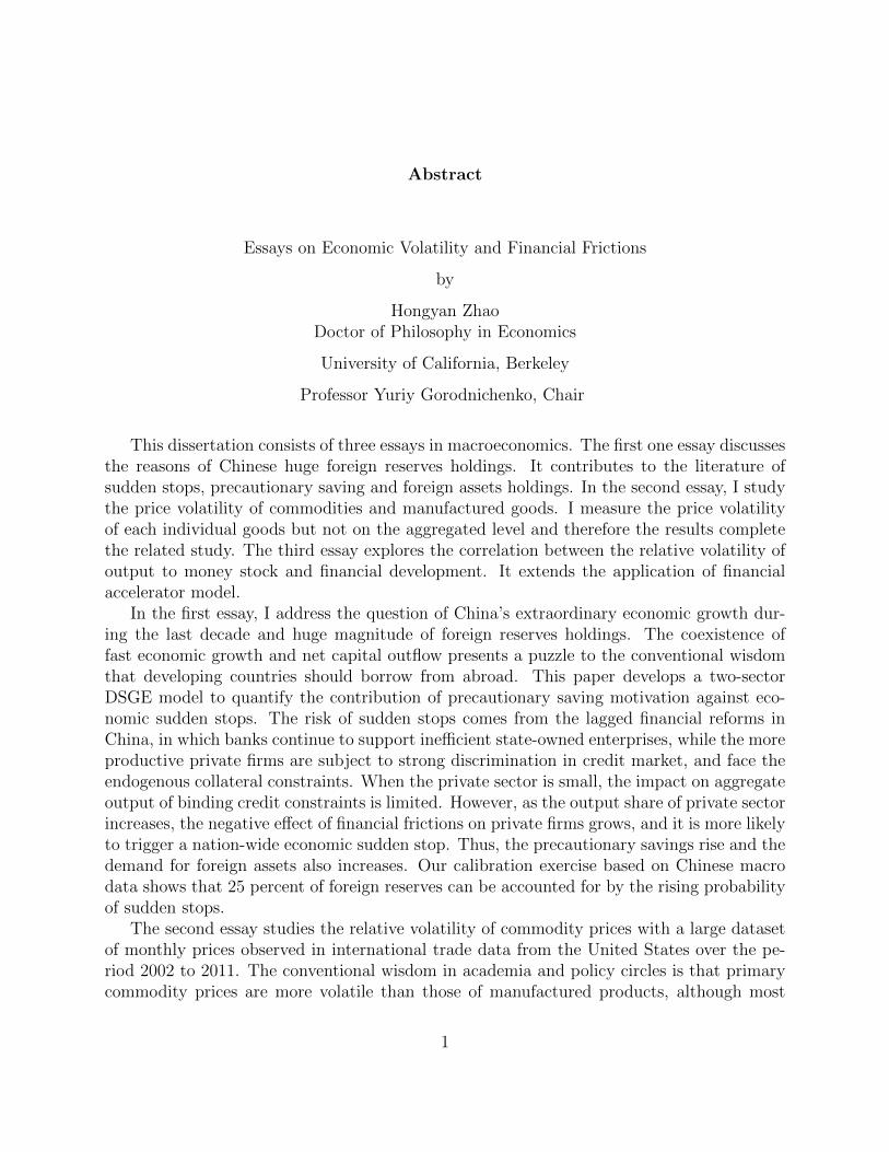
This dissertation consists of three essays in macroeconomics. The first one essay discussesthe reasons of Chinese huge foreign reserves holdings. It contributes to the literature ofsudden stops, precautionary saving and foreign assets holdings. In the second essay, I studythe price volatility of commodities and manufactured goods. I measure the price volatilityof each individual goods but not on the aggregated level and therefore the results completethe related study. The third essay explores the correlation between the relative volatility ofoutput to money stock and financial development. It extends the application of financialaccelerator model.
In the first essay, I address the question of China’s extraordinary economic growth dur-ing the last decade and huge magnitude of foreign reserves holdings. The coexistence offast economic growth and net capital outflow presents a puzzle to the conventional wisdomthat developing countries should borrow from abroad. This paper develops a two-sectorDSGE model to quantify the contribution of precautionary saving motivation against eco-nomic sudden stops. The risk of sudden stops comes from the lagged financial reforms inChina, in which banks continue to support inefficient state-owned enterprises, while the moreproductive private firms are subject to strong discrimination in credit market, and face theendogenous collateral constraints. When the private sector is small, the impact on aggregateoutput of binding credit constraints is limited. However, as the output share of private sectorincreases, the negative effect of financial frictions on private firms grows, and it is more likelyto trigger a nation-wide economic sudden stop. Thus, the precautionary savings rise and thedemand for foreign assets also increases. Our calibration exercise based on Chinese macrodata shows that 25 percent of foreign reserves can be accounted for by the rising probabilityof sudden stops.
The second essay studies the relative volatility of commodity prices with a large datasetof monthly prices observed in international trade data from the United States over the pe-riod 2002 to 2011. The conventional wisdom in academia and policy circles is that primarycommodity prices are more volatile than those of manufactured products, although most
1
existing studies do not measure the relative volatility of prices of individual goods or com-modities. The literature tends to focus on trends in the evolution and volatility of ratios ofprice indexes composed of multiple commodities and products. This approach can be mis-leading. The evidence presented here suggests that, on average, prices of individual primarycommodities are less volatile than those of individual manufactured goods. Furthermore,robustness tests suggest that these results are not likely to be due to alternative productclassification choices, differences in product exit rates, measurement errors in the trade data,or the level of aggregation of the trade data. Hence the explanation must be found in therealm of economics, rather than measurement. However, the challenges of managing termsof trade volatility in developing countries with concentrated export baskets remain.
The third essay tries to understand why the relative volatility of nominal output tomoney stock is negatively related to countries’ financial development level from cross-countryevidence. In the paper I modify Bernanke et al. (1999)’s financial accelerator model byintroducing the classic money demand function. The calibration to US data shows that themodel is able to replicate this empirical pattern quite well. Given the same monetary shocks,countries with poorer financial system have larger output volatility due to the stronger effectof financial accelerator mechanism.
2

To my family, who made it possible,and to my dearest Liugang, who made it happen.
i

Acknowledgments
I would like to thank my advisor and committee chair, Yuriy Gorodnichenko, who hasguided me from the earliest stage of my research. Without his advice and encouragement, Iwould not have been able to finish the Ph.D. program. I would also like to thank committeemembers, Maurice Obstfeld, Demian Pouzo, and James Wilcox.
I wrote the third chapter as preparation for my oral exam. During those periods, Igot many helpful comments and suggestions from Professor Yuriy Gorodnichenko, FredericoFinan, Maurice Obstfeld, Demian Pouzo, and James Wilcox. The second chapter is what Ihave done as a summer intern in the International Monetary Fund in 2011. It is coauthoredwith Rabah Arezki in IMF and Daniel Lederman in World Bank. Not only thanks for theuseful comments from Rabah, but also many thanks for his encouragement and great supportto my application for IMF.
ii
Contents
Contents iv
List of Tables v
List of Figures vi
1 Capital Misallocation, Sudden Stop and Foreign Reserves in China 11.1 Introduction . . . . . . . . . . . . . . . . . . . . . . . . . . . . . . . . . . . . 11.2 Literature Review . . . . . . . . . . . . . . . . . . . . . . . . . . . . . . . . . 31.3 External Sector in China . . . . . . . . . . . . . . . . . . . . . . . . . . . . . 6
1.3.1 Foreign Debts . . . . . . . . . . . . . . . . . . . . . . . . . . . . . . . 61.3.2 Capital Flows and Reserve Asset . . . . . . . . . . . . . . . . . . . . 8
1.4 Model . . . . . . . . . . . . . . . . . . . . . . . . . . . . . . . . . . . . . . . 91.4.1 Preference . . . . . . . . . . . . . . . . . . . . . . . . . . . . . . . . . 91.4.2 Production . . . . . . . . . . . . . . . . . . . . . . . . . . . . . . . . 101.4.3 Solutions . . . . . . . . . . . . . . . . . . . . . . . . . . . . . . . . . . 14
1.5 Calibration . . . . . . . . . . . . . . . . . . . . . . . . . . . . . . . . . . . . 151.5.1 Parameters Estimation . . . . . . . . . . . . . . . . . . . . . . . . . . 151.5.2 Shocks and Estimation . . . . . . . . . . . . . . . . . . . . . . . . . . 17
1.6 Results . . . . . . . . . . . . . . . . . . . . . . . . . . . . . . . . . . . . . . . 171.6.1 Long Run Moments of Major Variables . . . . . . . . . . . . . . . . . 171.6.2 Sudden Stop Event Simulation . . . . . . . . . . . . . . . . . . . . . . 181.6.3 Effects of Relative Productivity . . . . . . . . . . . . . . . . . . . . . 191.6.4 Effects of Financial Development . . . . . . . . . . . . . . . . . . . . 20
1.7 Conclusions . . . . . . . . . . . . . . . . . . . . . . . . . . . . . . . . . . . . 20
2 The Relative Volatility of Commodity Prices: A Reappraisal 362.1 Introduction . . . . . . . . . . . . . . . . . . . . . . . . . . . . . . . . . . . . 362.2 Data . . . . . . . . . . . . . . . . . . . . . . . . . . . . . . . . . . . . . . . . 382.3 Main Results . . . . . . . . . . . . . . . . . . . . . . . . . . . . . . . . . . . 40
iii
2.3.1 Product “Re-Classification” . . . . . . . . . . . . . . . . . . . . . . . 402.3.2 Formal Tests of CDF Stochastic Dominance . . . . . . . . . . . . . . 40
2.4 Robustness . . . . . . . . . . . . . . . . . . . . . . . . . . . . . . . . . . . . 412.4.1 Product Destruction . . . . . . . . . . . . . . . . . . . . . . . . . . . 422.4.2 Volatility of Quantities . . . . . . . . . . . . . . . . . . . . . . . . . . 422.4.3 Homogeneous versus Differentiated Products . . . . . . . . . . . . . . 432.4.4 Measurement Errors . . . . . . . . . . . . . . . . . . . . . . . . . . . 432.4.5 Level of Aggregation and Product Varieties in the Trade Nomenclature 44
2.5 Conclusions . . . . . . . . . . . . . . . . . . . . . . . . . . . . . . . . . . . . 45
3 The Relative Output Volatility and Financial Development 583.1 Introduction . . . . . . . . . . . . . . . . . . . . . . . . . . . . . . . . . . . . 583.2 Literature Review . . . . . . . . . . . . . . . . . . . . . . . . . . . . . . . . . 603.3 Model . . . . . . . . . . . . . . . . . . . . . . . . . . . . . . . . . . . . . . . 61
3.3.1 Financial Friction . . . . . . . . . . . . . . . . . . . . . . . . . . . . . 613.3.2 Household . . . . . . . . . . . . . . . . . . . . . . . . . . . . . . . . . 623.3.3 Enterprise Sector . . . . . . . . . . . . . . . . . . . . . . . . . . . . . 633.3.4 Log-linearized Equations . . . . . . . . . . . . . . . . . . . . . . . . . 65
3.4 Simulations . . . . . . . . . . . . . . . . . . . . . . . . . . . . . . . . . . . . 663.4.1 Parameters and Coefficients . . . . . . . . . . . . . . . . . . . . . . . 663.4.2 Simulation Results . . . . . . . . . . . . . . . . . . . . . . . . . . . . 673.4.3 Parameters Sensitivity Check . . . . . . . . . . . . . . . . . . . . . . 673.4.4 Quantitative Analysis . . . . . . . . . . . . . . . . . . . . . . . . . . . 68
3.5 Conclusions . . . . . . . . . . . . . . . . . . . . . . . . . . . . . . . . . . . . 68
A Appendices 84A.1 Lists of Commodities under the IMF Primary Commodity Price Tables and
UNCTAD Classifications . . . . . . . . . . . . . . . . . . . . . . . . . . . . . 84A.2 The Case with Investment Delay . . . . . . . . . . . . . . . . . . . . . . . . 84A.3 Other Shocks . . . . . . . . . . . . . . . . . . . . . . . . . . . . . . . . . . . 85A.4 Parameters Sensitivity Check . . . . . . . . . . . . . . . . . . . . . . . . . . 85
iv
List of Tables
1.1 China’s External Debt, 2001-2011 . . . . . . . . . . . . . . . . . . . . . . . . 211.2 Structure of China International Investment Position . . . . . . . . . . . . . 221.3 Chinese Holdings of U.S. Securities . . . . . . . . . . . . . . . . . . . . . . . 231.4 Values of Parameters . . . . . . . . . . . . . . . . . . . . . . . . . . . . . . . 241.5 Moments for Exogenous Variables . . . . . . . . . . . . . . . . . . . . . . . . 251.6 Comparison of Business Cycle Moments in the Model and Data . . . . . . . 26
2.1 Price Volatility by Harmonized System Groups . . . . . . . . . . . . . . . . . 472.2 Price Volatility Using Alternate Goods Classification . . . . . . . . . . . . . 482.3 Goods Entry and Exit . . . . . . . . . . . . . . . . . . . . . . . . . . . . . . 492.4 CDFs of Price Volatilities and the Level of Aggregation of Trade Data . . . . 50
3.1 Standard Deviations of Money and Nominal GDP Growth Rates (Annual Data) 703.2 Standard Deviations of Money and Nominal GDP Growth Rates (Quarterly
Data) . . . . . . . . . . . . . . . . . . . . . . . . . . . . . . . . . . . . . . . 713.3 Values of Parameters . . . . . . . . . . . . . . . . . . . . . . . . . . . . . . . 72
v
List of Figures
1.1 Foreign Reserves Ratio to GDP and Private Firms Output Share in China(1980-2010) . . . . . . . . . . . . . . . . . . . . . . . . . . . . . . . . . . . . 27
1.2 Liabilities-to-Assets Ratio of Industrial Firms (2000) . . . . . . . . . . . . . 281.3 External Debt in China (1985-2011) . . . . . . . . . . . . . . . . . . . . . . . 291.4 The Compostion of Annual Capital Inflows in China 1982-2011 (%) . . . . . 301.5 Simulated Sudden Stop Events Dynamics . . . . . . . . . . . . . . . . . . . . 311.6 Sudden Stops Probability and Foreign Reserves Holdings . . . . . . . . . . . 321.7 Current China’s Position in the Calibrated Model . . . . . . . . . . . . . . . 331.8 Savings by Sectors (%) . . . . . . . . . . . . . . . . . . . . . . . . . . . . . . 341.9 The Effect of Financial Constraint . . . . . . . . . . . . . . . . . . . . . . . . 35
2.1 Volatility of Aggregate Price Indices Using IMF Commodity Indices . . . . . 512.2 Volatility of Aggregate Price Indices using UNCTAD Commodity Indices . . 522.3 Cumulative Distribution Functions of Price Volatility for Goods with Unin-
terrupted Price Series . . . . . . . . . . . . . . . . . . . . . . . . . . . . . . . 532.4 Cumulative Distribution Functions of Price Volatility for Selected Manufac-
tured Products . . . . . . . . . . . . . . . . . . . . . . . . . . . . . . . . . . 542.5 Cumulative Distribution Function of Price Volatility for Goods Available for
the Whole Period . . . . . . . . . . . . . . . . . . . . . . . . . . . . . . . . . 552.6 Cumulative Distribution Function of Volatility of Import Quantities . . . . . 562.7 Cumulative Distribution Function of Price Volatility for Differentiated and
Homogenous Goods . . . . . . . . . . . . . . . . . . . . . . . . . . . . . . . . 57
3.1 Financial Development and Volatility Ratio . . . . . . . . . . . . . . . . . . 733.2 Financial Development and Volatility Ratio (Developed Countries) . . . . . . 743.3 Impulse Response of Monetary Shock-Basic Case: µ = 0.12 . . . . . . . . . . 753.4 Impulse Response of Monetary Shock-Alternative Case: µ = 0.52 . . . . . . . 763.5 Simulated Financial Development Measure and Volatility Ratio . . . . . . . 773.6 Simulated Financial Development Measure and Volatility Ratio in China . . 783.7 Simulated Financial Development Measure and Ratio of Credit to Output . . 79
vi
3.8 Simulated Ratio of Credit to Output and Volatility Ratio . . . . . . . . . . . 803.9 Impulse Responses of Monetary Shock with Investment delay: µ = 0.12 . . . 813.10 Comparison under Different Shocks . . . . . . . . . . . . . . . . . . . . . . . 823.11 Parameters Sensitivity Check . . . . . . . . . . . . . . . . . . . . . . . . . . 83
vii
Chapter 1
Capital Misallocation, Sudden Stop andForeign Reserves in China
1.1 Introduction
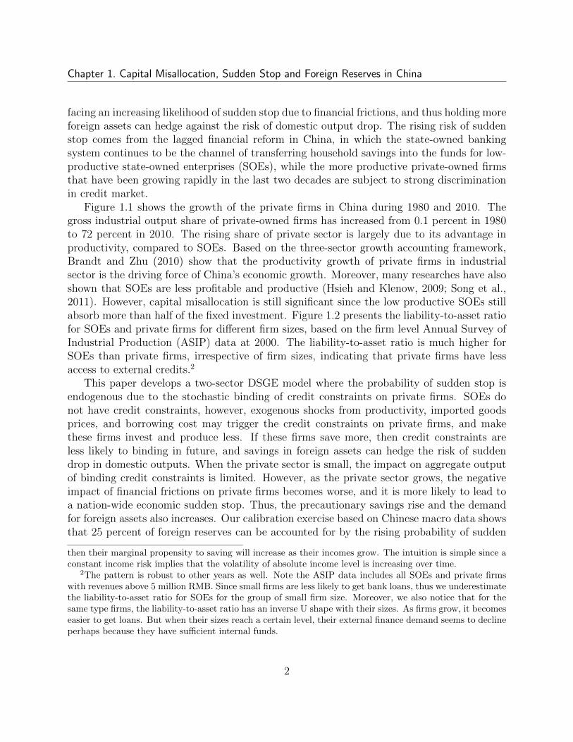
The rising stocks of foreign reserves in emerging economies in the last decade have stimulateda considerable debate both in policy institutions and academic circle, because it has beenconsidered as a major force of global imbalance and housing price bubble. The reserves toGDP ratio has increased from about 4.7 percent in 1995 to 14.7 percent in 2011, and the surgeof reserves in the emerging and developing economies is even more striking. The reserves toGDP ratio in those countries has risen from about 8 percent to 27 percent. Initially Dooleyet al. (2003, 2004a,b) take the view of modern mercantilism-the accumulation of reserves ispart of the development strategy for developing countries that pursue an export-led growthsupported by undervalued exchange rates and capital controls. Recently economists areleaning toward the precautionary view of reserves accumulation-emerging economies treatreserves as a war chest against uninsured risks associated with financial frictions and suddenstops (Aizenman and Lee, 2007; Durdu et al., 2009; Obstfeld et al., 2010).
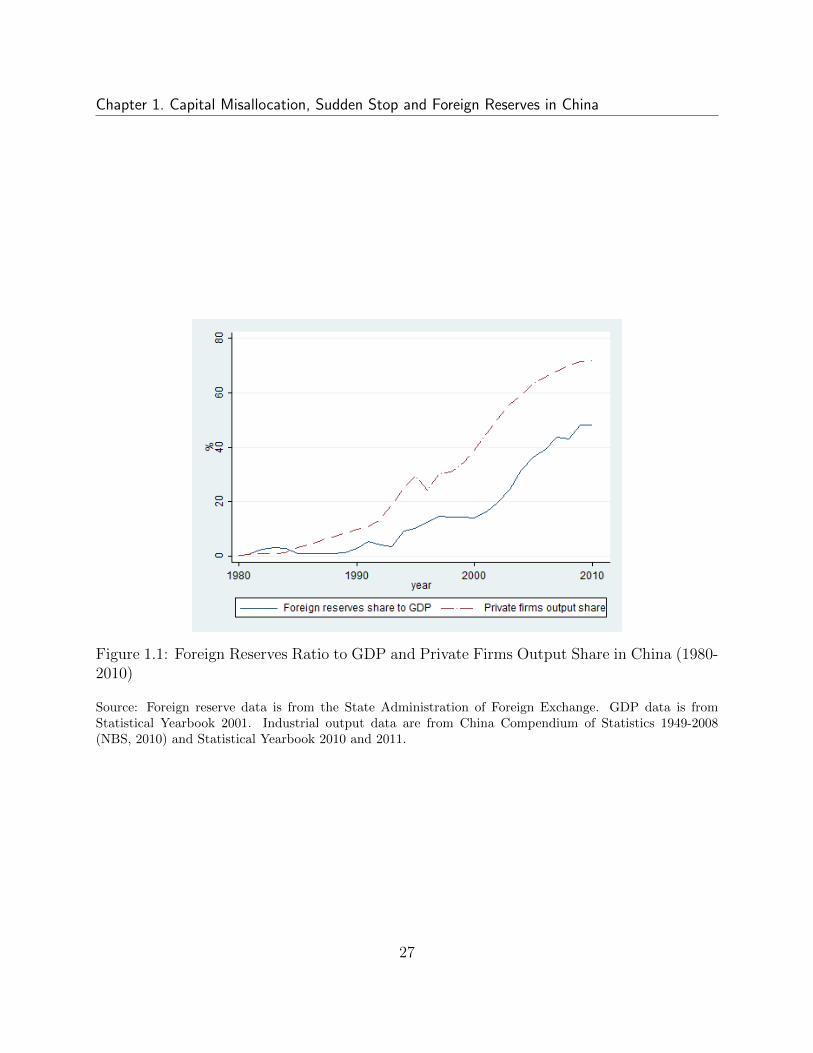
Undoubtedly China has been the focus of this debate because the country has held thelargest amount of foreign reserves in the world; one single country has contributed more than30 percent of total world reserves by 2011. As a result of market oriented reform, China hasachieved miraculous economic growth in the last three decades. Meanwhile, the reserves toGDP ratio has increased dramatically to about 48 percent by the end of 2010 (Figure 1.1),which is very high even among those emerging and developing countries. Most of studieson China attribute this feature to the high saving rates (Song et al., 2011), however, nosystematic exercise has been carried out to quantify the precautionary motivation of reserveassets except Wen (2011).1 Our paper develops a quantitative framework where China is
1Wen (2011) argues that if entrepreneurs face constant uninsured income risk despite long-run growth,
1
Chapter 1. Capital Misallocation, Sudden Stop and Foreign Reserves in China
facing an increasing likelihood of sudden stop due to financial frictions, and thus holding moreforeign assets can hedge against the risk of domestic output drop. The rising risk of suddenstop comes from the lagged financial reform in China, in which the state-owned bankingsystem continues to be the channel of transferring household savings into the funds for low-productive state-owned enterprises (SOEs), while the more productive private-owned firmsthat have been growing rapidly in the last two decades are subject to strong discriminationin credit market.
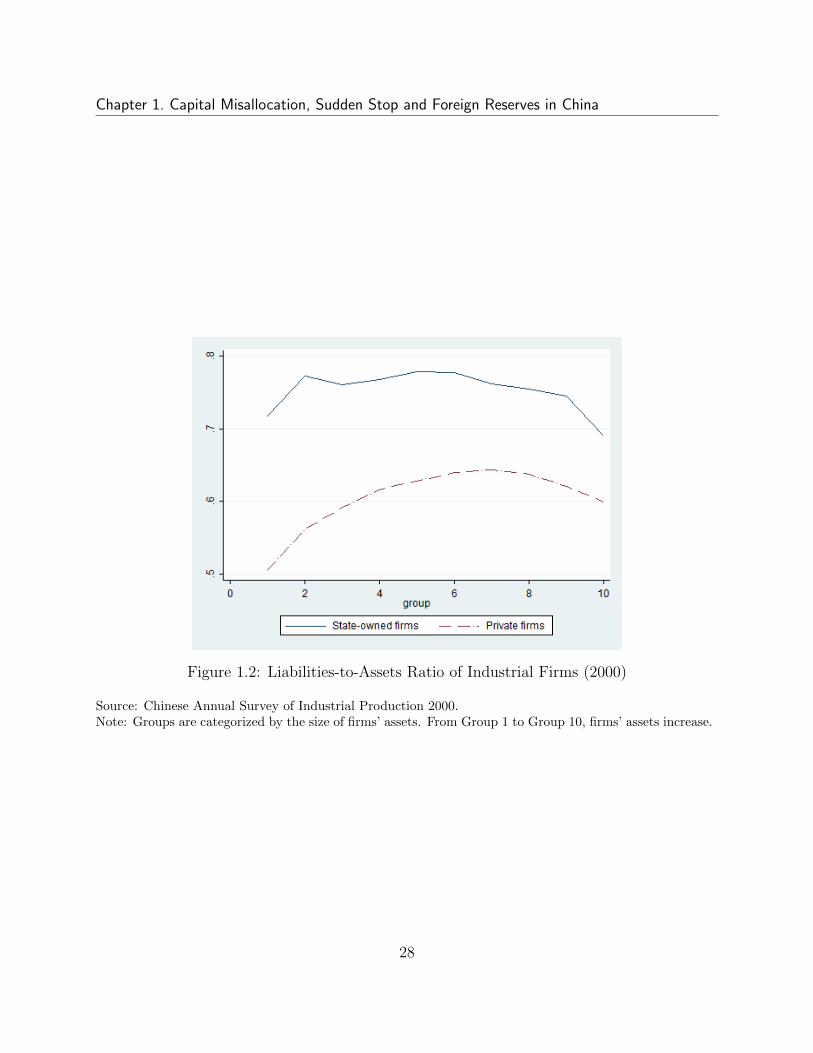
Figure 1.1 shows the growth of the private firms in China during 1980 and 2010. Thegross industrial output share of private-owned firms has increased from 0.1 percent in 1980to 72 percent in 2010. The rising share of private sector is largely due to its advantage inproductivity, compared to SOEs. Based on the three-sector growth accounting framework,Brandt and Zhu (2010) show that the productivity growth of private firms in industrialsector is the driving force of China’s economic growth. Moreover, many researches have alsoshown that SOEs are less profitable and productive (Hsieh and Klenow, 2009; Song et al.,2011). However, capital misallocation is still significant since the low productive SOEs stillabsorb more than half of the fixed investment. Figure 1.2 presents the liability-to-asset ratiofor SOEs and private firms for different firm sizes, based on the firm level Annual Survey ofIndustrial Production (ASIP) data at 2000. The liability-to-asset ratio is much higher forSOEs than private firms, irrespective of firm sizes, indicating that private firms have lessaccess to external credits.2
This paper develops a two-sector DSGE model where the probability of sudden stop isendogenous due to the stochastic binding of credit constraints on private firms. SOEs donot have credit constraints, however, exogenous shocks from productivity, imported goodsprices, and borrowing cost may trigger the credit constraints on private firms, and makethese firms invest and produce less. If these firms save more, then credit constraints areless likely to binding in future, and savings in foreign assets can hedge the risk of suddendrop in domestic outputs. When the private sector is small, the impact on aggregate outputof binding credit constraints is limited. However, as the private sector grows, the negativeimpact of financial frictions on private firms becomes worse, and it is more likely to lead toa nation-wide economic sudden stop. Thus, the precautionary savings rise and the demandfor foreign assets also increases. Our calibration exercise based on Chinese macro data showsthat 25 percent of foreign reserves can be accounted for by the rising probability of sudden
then their marginal propensity to saving will increase as their incomes grow. The intuition is simple since aconstant income risk implies that the volatility of absolute income level is increasing over time.
2The pattern is robust to other years as well. Note the ASIP data includes all SOEs and private firmswith revenues above 5 million RMB. Since small firms are less likely to get bank loans, thus we underestimatethe liability-to-asset ratio for SOEs for the group of small firm size. Moreover, we also notice that for thesame type firms, the liability-to-asset ratio has an inverse U shape with their sizes. As firms grow, it becomeseasier to get loans. But when their sizes reach a certain level, their external finance demand seems to declineperhaps because they have sufficient internal funds.
2

Chapter 1. Capital Misallocation, Sudden Stop and Foreign Reserves in China
stop.Our study also shows that improvement of financial constraints on private firms will
reduce the risk of sudden stop significantly, as well as the precautionary saving in foreignreserves. This finding has important policy implication for the Chinese government. To easethe external imbalance of Chinese economy, the government needs to remove the barriers tocredit market for private firms in future.
Our paper is close to Mendoza (2010) and Durdu et al. (2009) where they also argue thatthe high stocks of foreign reserves held by emerging economies act as a war chest againstthe risks of sudden stop. However, their models do not have two sectors in which theyhave different access to credit market, thus there is no capital misallocation across sectors orcomposition effect of production and probability of sudden stop. In this sense, our research isalso complementary to the literature of capital misallocation (Hsieh and Klenow, 2009; Songet al., 2011), in which most of current studies focus on the impact of capital misallocationon aggregate productivity. However, this paper shows that capital misallocation also hasimplications on economic fluctuations.
We discuss the related literature in section 1.2 and China’s foreign debts, capital flowsand foreign exchange reserves in section 1.3. Section 1.4 discusses the model set up and howto solve it. Section 1.5 summarizes the parameters’ estimation and introduces the exogenousshocks to the model. Section 1.6 presents the simulation results for China’s case and insection 1.7 we conclude.
1.2 Literature Review
The rising stocks of foreign reserves in emerging economies in the last decade have prompteda considerable debate. Among these explanations, Dooley et al. (2003, 2004a,b) take the viewof modern mercantilism-the accumulation of reserves is part of the development strategy fordeveloping countries that pursue an export-led growth supported by undervalued exchangerates and capital controls. They also claim that official capital outflows in the form ofaccumulation of reserve asset are not only a necessary policy to maintain the undervaluedexchange rates, but also serve as a “collateral” for encouraging foreign direct investment.
However, this explanation may not hold for the case of China. First, it is unlikelyto maintain undervalued exchange rates for a median run or long run by using monetarypolicy, as shown in many studies that monetary policies usually do not have long run effecton exchange rates and outputs (Aizenman and Lee, 2008). Moreover, Cheung et al. (2007)have not found statistical significant evidence showing that China’s currency is undervalued,in terms of the deviation of the price level from the international trend, based on a detailedexamination of the price level data for a panel of more than 100 countries over the periodof 1975-2004. Second, the impact of undervalued exchange rates on trade surplus is notuncontroversial. The extant literature studying the price and income elasticities of Chinese
3
Chapter 1. Capital Misallocation, Sudden Stop and Foreign Reserves in China
trade flows are relatively small, if there was a consensus among researchers (Cheung et al.,2010; Xing, 2012). In fact, previous research has indicated a mixed evidence of the effect ofan appreciation of the Renminbi on Chinese trade flow, and sometimes researchers even finda wrong sign of the exchange rate elasticity on imports (e.g. see the discussion in Thorbeckeand Smith (2012)). One important reason is that processing trade in China contributesabout a half to Chinese total trade volume, so a large portion of Chinese imports is forre-export. An appreciation of the RMB that reduces exports will also reduce imports thatare used to produce products for re-export. Thus, the impact of exchange rates on tradebalance is ambiguous. Third, a systematic comparison of precautionary versus mercantilistviews of foreign reserves requires a detailed econometric analysis. Based on a panel of 49developing countries including China over the period 1908-2000, Aizenman and Lee (2007)have found supporting evidence for precautionary motives, while the role of mercantilism isquantitatively limited.
The second possible explanation of rising reserves in China is international portfoliodiversification. In the last three decades, China has grown from a neglectable player inthe world market to the largest exporter in the world. However, residential Chinese stillhave limited access to foreign assets, due to the government capital control. Thus, as analternative way to diversify the country’s portfolio, it might be optimal for the government toincrease the holdings of foreign reserves. However, this portfolio diversification view cannotstand after a careful examination. The objective of portfolio diversification is to maximizethe expected return of asset holdings; however, the dramatic accumulation of reserves bythe Chinese government was accompanied by a significant depreciation of the U.S. dollar inthe last decade. Because the majority of reserve assets are in U.S. dollar and highly liquidgovernment bonds with low returns, the capital loss due to the depreciation of the dollaris tremendous.3 Moreover, this capital loss is even foreseeable because in early 2004 thepresident of Federal Reserves, Alan Greenspan delivered a warning message that China wasfacing an increasing US dollar “concentration risk” as its reserves increased quickly. It isdifficult to reconcile the low return of the dollar assets and the fast accumulation of reserves,if precautionary incentive does not play a significant role.
The third popular explanation is the “saving glut” hypothesis (Caballero et al., 2008a).Our model also follows this line to explain the rising saving rate and foreign reserves, andwe also note that there is no shortage of theories of savings behavior in the literature.
China’s national saving rates have been increasing from 38 percent in 2000 to 53 percentin 2007 (Yang et al., 2011). We observe the similar pattern in the experiences of the EastAsian economies, such as Japan in the 1970s and Korea and Taiwan in the 1980s, as well
3A back-of-the-envelope calculation suggests that the capital loss of Chinese reserves due to the dollardepreciation since 2005, can easily exceed 5 percent of its annual GDP: 830 ∗ 0.7 ∗ (1− 6.3/8.1)/2400 = 5.3percent, where 830 billion dollars were the reserves by the end of 2005, 70 percent is the proportion of theU.S. dollar assets in the reserves (Sheng, 2011), 8.1 was the RMB/dollar rate at the end of 2005, 6.3 is thecurrent exchange rate of RMB, and 2400 billion dollars was China’s nominal GDP in 2005.
4
Chapter 1. Capital Misallocation, Sudden Stop and Foreign Reserves in China
as other BRIC countries (Brazil, Russia, India, and China) in recent years. Thus, the co-movement of high economic growth and high saving rate is not new to China. This presentsa puzzle to the classical Life Cycle Hypothesis (Modigliani, 1970; Modigliani and Cao, 2004),because it predicts that households tend to save less when they expect high income growthin future. Thus, Chamon and Prasad (2010) argue that because Chinese government did notprovide systematic health insurance and unemployment insurance, household expenditureon health care, education and housing is rising as well. This uninsured income risk andunexpected expenditures render the Chinese households to save more even though theirincomes increase.4 Wen (2011) develops a quantitative model showing that this precautionarysaving motivation can account for the rising trade surplus and foreign reserves in China aswell.
Moreover, Wei and Zhang (2011) provide a novel and interesting theory to account forthe rising saving rates in China. They argue that as the sex ratio (the number of men perwoman in the premarital cohort) rises, families with sons raise their saving rate to promotetheir sons’ standing on marriage market. They show that this unbalanced sexual bias canaccount for about half of the actual increase in the household savings rate during 1990 and2007. Based on this idea, Du and Wei (2010) develop a quantitative OLG model of openeconomies, and their calibration exercise show that the cross country difference in sex ratiocan account for more than 1/2 of the actual current account imbalances observed in theinternational data.
Our explanation relies on precautionary saving incentive, but emphasizes on the role offinancial friction. In this sense our research is close to Durdu et al. (2009), which argue thatemerging economies are practicing a New Mercantilism that takes foreign reserves as a warchest against future economic sudden stops due to debt limit constraint in a more financialintegrated world. Because reserves accumulation will decrease the probability of suddenstops in the long run, emerging economies prefer to hold more foreign assets although thereturn might be very low. The authors find that financial globalization and risk of suddenstop may account for the rising reserves in emerging economies; however, output volatilityis not the driving force of precautionary saving since the data for countries experiencedwith sudden stops in history shows that their output volatility did not increase substantiallybefore sudden stops.
Jeanne and Ranciere (2011) develop a tractable model of the optimal level of foreignreserves for a small open economy hedging against sudden stops in capital inflows. However,different from our model where the probability of sudden stop is endogenous, they treatforeign reserves as a state-contingent insurance contract that helps consumers to smooth
4Recently, Song and Yang (2010) develop an explanation to reconcile the co-movement of saving ratesand economic growth with the Life Cycle theory. They argued that in fast-growing economies, the youngercohorts earn much more than the elders as they enter labor market, but their income growth rates are lowerthan the elders’. This flatten life-time income profile encourages the younger cohorts to save more, thus theaggregate household saving rate also increases as the aggregate income increases.
5
Chapter 1. Capital Misallocation, Sudden Stop and Foreign Reserves in China
their consumptions between their sudden stop state and normal state with pre-specifiedprobabilities. They find that the reserves accumulation in emerging market Asia can beexplained only if these countries have a high level of risk aversion or a large anticipatedoutput drop of sudden stops. Their calibration implies an optimal level of reserves of 9.1percent of GDP.
Obstfeld et al. (2010) extend this precautionary saving motivation and focus on the roleof foreign reserves in hedging the risk of domestic financial instability and exchange rates ina world of rising financial globalization. The central banks of emerging economics attempt toease domestic illiquidity by acting as lenders of last resort, in the case of dramatic and vastcapital flight due to various reasons including economic sudden stops and large devaluationof exchange rates. This explanation is one of possible reasons for China’s huge reserves, butquantitatively it is not sufficient as the authors admitted that their empirical model left asubstantial fraction of China’s reserves unexplained in 2003-2004, however, it is the timethat China’s reserves accumulation started to accelerate.
Our research is also related to Song et al. (2011) where financial frictions play a centralrole in misallocation of capital between state-owned firms and private firms. In their model,more productive private firms have more severe credit constraints and the banking systemin China prefers state-owned firms. However, saving in foreign assets in their model ismechanical as state-owned firms shrink and their demand for bank loans decreases, thusbanks can only hold foreign reserves as their assets. In our model, foreign reserves are usedto hedge domestic production risk of sudden stop, thus this paper is complementary to theirstudies.
1.3 External Sector in China
The risk of sudden stop is certainly associated with the country’s exposure to foreign capitalmarket, especially short term capital flows. Moreover, if the governments plan to use foreignreserves to hedge against the risk of massive capital outflow and economic sudden stops, thenthe majority of reserves must be highly liquid assets. This section provides a careful exami-nation of China’s external sector including the foreign debts, capital flows, and compositionof foreign reserves. As a result, we find that the private sector in China essentially involvedsignificantly in the foreign capital inflow, both in terms of foreign direct investment andshort term foreign debts, and the main component of reserves is highly liquid governmentbonds.
1.3.1 Foreign Debts
China has been very cautious about taking on external debt. There has been little sovereignborrowing and enterprises have been discouraged from taking on external debt except for
6
Chapter 1. Capital Misallocation, Sudden Stop and Foreign Reserves in China
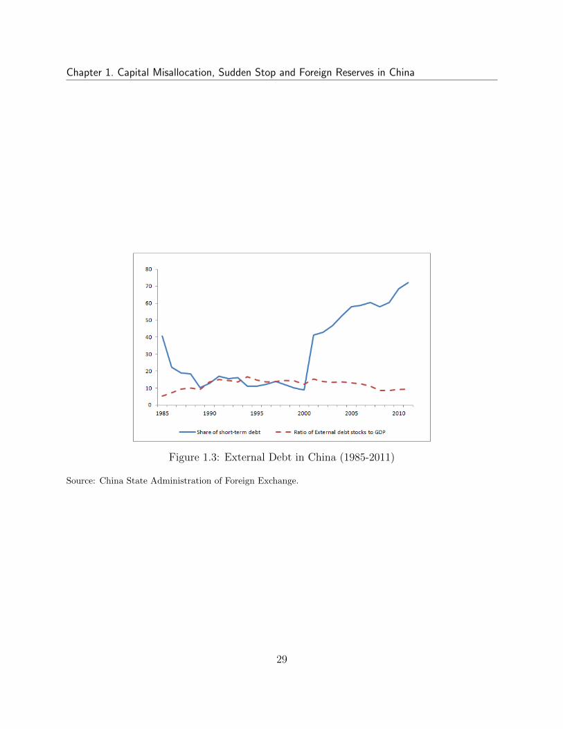
foreign owned enterprises. As a result, although the stocks of external debt significantlyincreased, the ratio of external debt stock over GDP has never exceeded 20 percent since1981 (Table 1.1 and Figure 1.3). Since GDP includes a large portion of nontradeable goods,sometimes people prefer to use the ratio of external debt to export goods and services(tradeable goods) as a measure of countries’ debt-paying ability. The third row in Table 1.1presents this index indicating a decline of the relative size of external debts since 2001, andthe index of China was below the average of emerging economies. However, since processingexports contribute about a half of aggregated trade in China, and their value added is small.Thus, we also compute the ratio of external debt to ordinary export, and this index ismuch higher; however, it declined over time as well. The common declining pattern in thesethree indices implies that the Chinese government aimed to control the size of external debt,particularly after the East Asian financial crisis. Given the limited size of external debt,it seems that one does not need to worry about China’s external debt; however, a closeexamination hints that this might not be true.
First, it is not just the level of external debt but also the maturity structure and typesof debts that have been shown to be associated with currency and financial crisis. Countriesthat have more short-term debt relative to long-term debt tend to be more susceptible to suchcrisis. At this point, one significant change is that the share of short-term debt in China’stotal external debt has risen dramatically, from 9 percent in 2000 to an unprecedented level63 percent in 2011. Moreover, a significant part of this rising in the relative importanceof short-term debt since 2001 can be accounted for by the surge in trade credits.5 Tradecredits contributed 27 percent of total external debt in 2001, and the share of trade creditshas increased up to 36 percent. In addition, many external debt borrowed by financialinstitutions are also related to trade, such as Usance Credit. According to a recent reportby the State Administration of Foreign Exchange, trade credit contributed about 84 percentof the rising short-term debt during 2001 and 2010 (SAFE, 2010, p.47.).
One important feature of the rising external debt inflow is that it is mainly driven bythe private sector. The external debts taken by the Chinese government have been keptat a stable level and thus its share in debt stocks decreased from about a quarter in 2001to only 5 percent. Even if the Chinese-funded financial institutions are considered as apart of government sector, the private sector still contributed more than 60 percent of totalexternal debts in recent years because trade credits are also mainly driven by private firms.In particular, within the private sector, foreign funded enterprises play a significant andactive role in taking on registered external debts, partly because they have better access toglobal financial market, partly because the Chinese government has more restrictive policiesfor Chinese-funded firms to borrow overseas. Chinese owned private firms are more likely touse trade credits to finance their liquidity because the government regulation on trade credit
5The statistics of short-term debts are not comparable before and after 2001, because trade credits within3 months were not counted in the short term debts until 2001. Thus, the short term debts before 2001 wereunderreported.
7
Chapter 1. Capital Misallocation, Sudden Stop and Foreign Reserves in China
is relatively limited, compared with those restrictions on registered debt.Overall, the stock of external debt itself may not be the source of concern. However, the
maturity structure of external debt and its concentration on trade credits and private sectorrequire particular attention. Because the Chinese currency RMB is not convertible, themajority of foreign debts are in foreign currency, particularly in US dollar. If there occurreda short-term liquid shock on external debts, it would certainly hurt China’s exports in shortrun, and further on foreign direct investment in the long run as well. This feature is verysimilar to developing countries that have experienced sudden stops, such as Malaysia andKorea in 1997. Given the important role of export and FDI in promoting economic growthin China, it might not be groundless to suspect a financial or currency crisis. In fact, theworrisome about a hard-landing of China’s economy never ends in newspapers and media.
1.3.2 Capital Flows and Reserve Asset
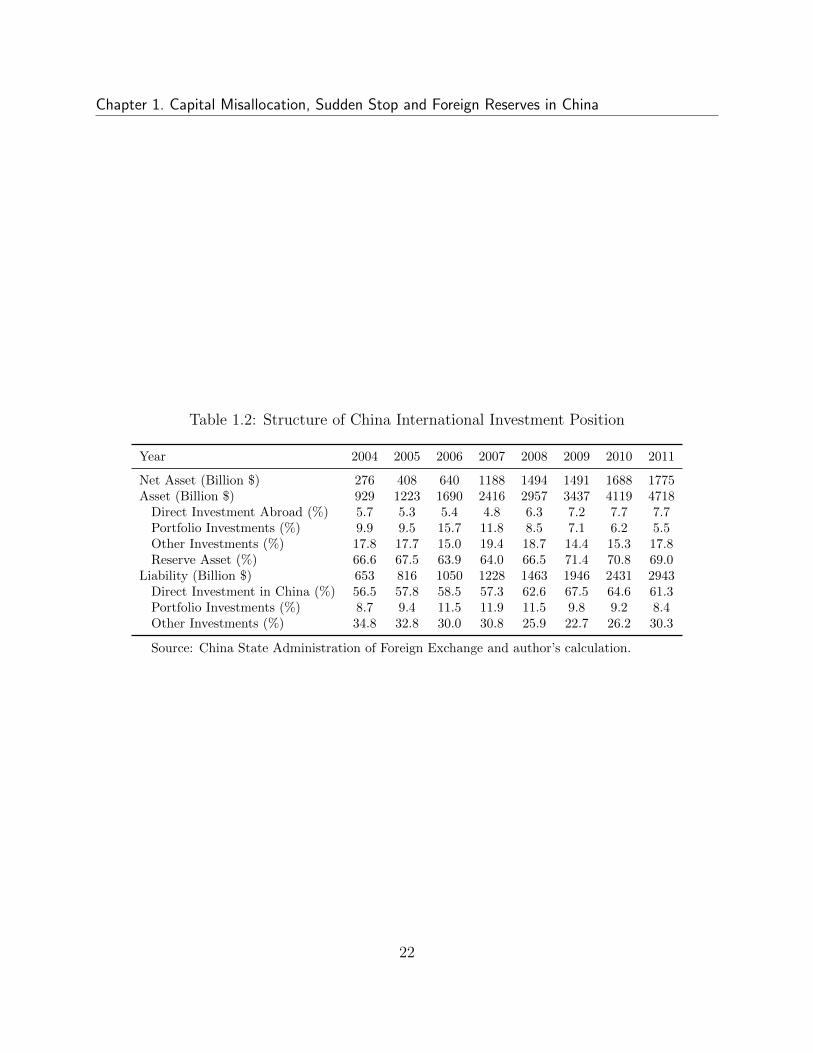
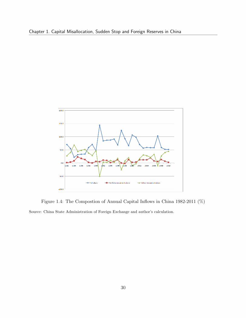
The Chinese government took a conservative approach to the capital flow liberalization. Inthe last two decades the country was successful in encouraging foreign capital inflows in theform of direct investment, as it has emerged as the largest FDI receipting country amongdeveloping countries. Table 1.2 shows that inward FDI has contributed about 60 percentof total stocks of capital inflow during 2004 and 2011. A longer period covering 1982-2011in Figure 1.4 shows that the annual FDI inflow is more important in 1990s than in 2000s,and other investments including trade credits, bank loans and currency and deposits werecatching up in recent years, but the share of portfolio investment kept stable. This impliesthat the Chinese government was gradually lifting the capital controls in financial sector,but took a prudential step in liberalizing the restrictions on portfolio investment.
People do not worry about the current pattern of Chinese capital inflows, given its strongregulations and controls on financial capital. The problem is how to liberalize the capitaland financial account and its embedded risk of changes of international investment positionafter financial liberalization.6
Table 1.2 also shows that the majority of China’s foreign assets are reserve asset, whichon average contributed about 67.5 percent to total asset during 2004 and 2011. Directinvestment abroad, porfolio and other investments play a minor role in its asset portfolio.Most of reserve assets are foreign exchange reserves held by the central bank. This is partlybecause the Chinese government had regulation on the holdings in foreign assets of residentialhouseholds and domestic firms, partly because investors expected the RMB would appreciatein the long run, thus the central bank had to buy foreign assets at the given exchange rate.
Although the Chinese government does not provide information of currency compositionand portfolio of its official foreign reserves, researchers have shown China held about two-thirds of its foreign exchange reserves in the U.S. dollar and more than one fifth in the
6See He et al. (2012) for a detailed discussion of the impact of capital account liberalization on China’scapital flows, international investment position and the value of the Chinese RMB.
8
Chapter 1. Capital Misallocation, Sudden Stop and Foreign Reserves in China
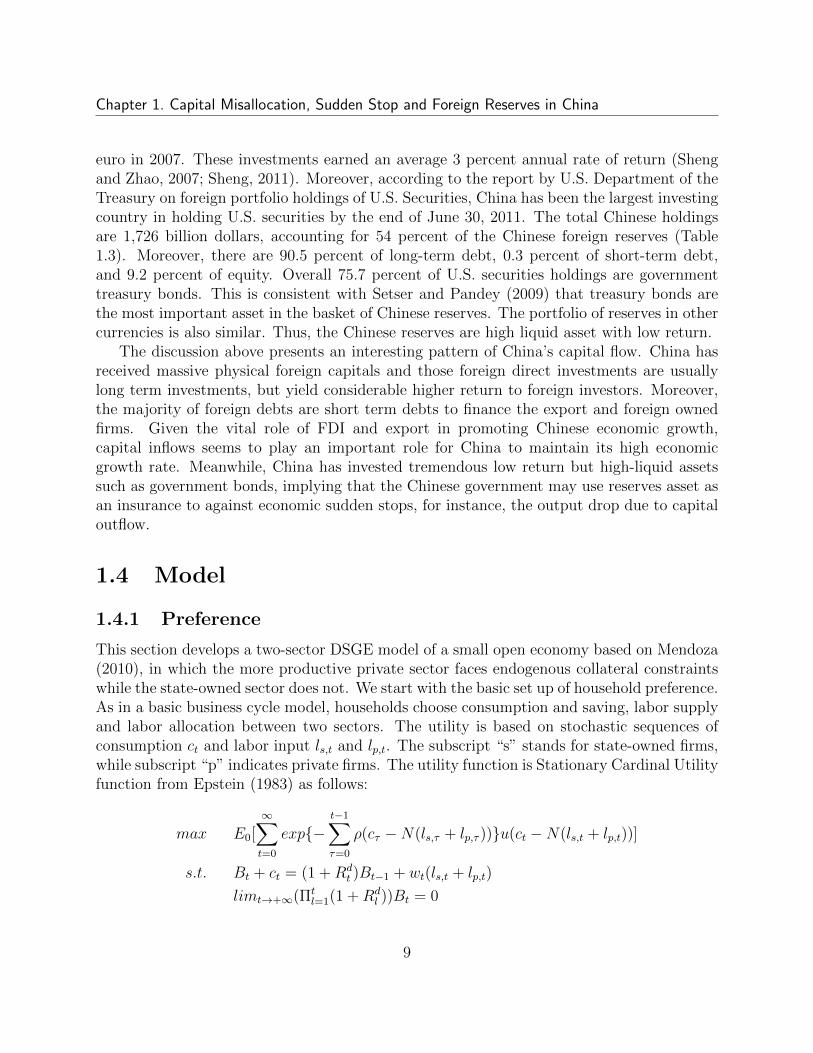
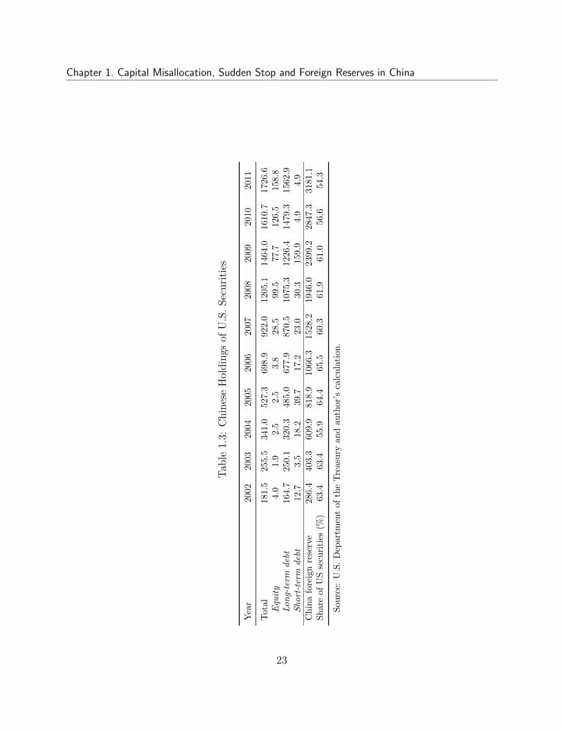
euro in 2007. These investments earned an average 3 percent annual rate of return (Shengand Zhao, 2007; Sheng, 2011). Moreover, according to the report by U.S. Department of theTreasury on foreign portfolio holdings of U.S. Securities, China has been the largest investingcountry in holding U.S. securities by the end of June 30, 2011. The total Chinese holdingsare 1,726 billion dollars, accounting for 54 percent of the Chinese foreign reserves (Table1.3). Moreover, there are 90.5 percent of long-term debt, 0.3 percent of short-term debt,and 9.2 percent of equity. Overall 75.7 percent of U.S. securities holdings are governmenttreasury bonds. This is consistent with Setser and Pandey (2009) that treasury bonds arethe most important asset in the basket of Chinese reserves. The portfolio of reserves in othercurrencies is also similar. Thus, the Chinese reserves are high liquid asset with low return.
The discussion above presents an interesting pattern of China’s capital flow. China hasreceived massive physical foreign capitals and those foreign direct investments are usuallylong term investments, but yield considerable higher return to foreign investors. Moreover,the majority of foreign debts are short term debts to finance the export and foreign ownedfirms. Given the vital role of FDI and export in promoting Chinese economic growth,capital inflows seems to play an important role for China to maintain its high economicgrowth rate. Meanwhile, China has invested tremendous low return but high-liquid assetssuch as government bonds, implying that the Chinese government may use reserves asset asan insurance to against economic sudden stops, for instance, the output drop due to capitaloutflow.
1.4 Model
1.4.1 Preference
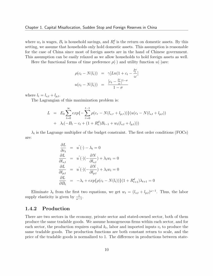
This section develops a two-sector DSGE model of a small open economy based on Mendoza(2010), in which the more productive private sector faces endogenous collateral constraintswhile the state-owned sector does not. We start with the basic set up of household preference.As in a basic business cycle model, households choose consumption and saving, labor supplyand labor allocation between two sectors. The utility is based on stochastic sequences ofconsumption ct and labor input ls,t and lp,t. The subscript “s” stands for state-owned firms,while subscript “p” indicates private firms. The utility function is Stationary Cardinal Utilityfunction from Epstein (1983) as follows:
max E0[∞∑t=0
exp−t−1∑τ=0
ρ(cτ −N(ls,τ + lp,τ ))u(ct −N(ls,t + lp,t))]
s.t. Bt + ct = (1 +Rdt )Bt−1 + wt(ls,t + lp,t)
limt→+∞(Πtl=1(1 +Rd
l ))Bt = 0
9
Chapter 1. Capital Misallocation, Sudden Stop and Foreign Reserves in China
where wt is wages, Bt is household savings, and Rdt is the return on domestic assets. By this
setting, we assume that households only hold domestic assets. This assumption is reasonablefor the case of China since most of foreign assets are in the hand of Chinese government.This assumption can be easily relaxed as we allow households to hold foreign assets as well.
Here the functional forms of time preference ρ(·) and utility function u(·)are:
ρ(ct −N(lt)) = γ[Ln(1 + ct −lωtω
]
u(ct −N(lt)) =[ct − lωt
ω]1−σ
1− σ
where lt = ls,t + lp,t.The Lagrangian of this maximization problem is:
L = E0
∞∑t=0
exp−t−1∑τ=0
ρ(cτ −N(ls,τ + lp,τ ))(u(ct −N(ls,t + lp,t))
+ λt(−Bt − ct + (1 +Rdt )Bt−1 + wt(ls,t + lp,t)))
λt is the Lagrange multiplier of the budget constraint. The first order conditions (FOCs)are:
∂L
∂ct= u
′(·)− λt = 0
∂L
∂ls,t= u
′(·)(− ∂N
∂ls,t) + λtwt = 0
∂L
∂lp,t= u
′(·)(− ∂N
∂lp,t) + λtwt = 0
∂L
∂Bt
= −λt + expρ(ct −N(lt))(1 +Rdt+1)λt+1 = 0
Eliminate λt from the first two equations, we get wt = (ls,t + lp,t)ω−1. Thus, the labor
supply elasticity is given by 1ω−1
.
1.4.2 Production
There are two sectors in the economy, private sector and stated-owned sector, both of themproduce the same tradable goods. We assume homogeneous firms within each sector, and foreach sector, the production requires capital kt, labor and imported inputs vt to produce thesame tradable goods. The production functions are both constant return to scale, and theprice of the tradable goods is normalized to 1. The difference in productions between state-
10
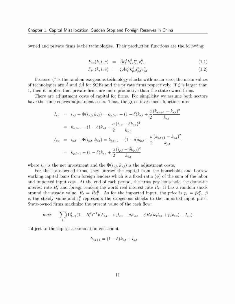
Chapter 1. Capital Misallocation, Sudden Stop and Foreign Reserves in China
owned and private firms is the technologies. Their production functions are the following:
Fs,t(k, l, v) = AεAt kβs,tl
αs,tv
ηs,t (1.1)
Fp,t(k, l, v) = ζAεAt kβp,tl
αp,tv
ηp,t (1.2)
Because εAt is the random exogenous technology shocks with mean zero, the mean valuesof technologies are A and ζA for SOEs and the private firms respectively. If ζ is larger than1, then it implies that private firms are more productive than the state-owned firms.
There are adjustment costs of capital for firms. For simplicity we assume both sectorshave the same convex adjustment costs. Thus, the gross investment functions are:
Is,t = is,t + Φ(is,t, ks,t) = ks,t+1 − (1− δ)ks,t +a
2
(ks,t+1 − ks,t)2
ks,t
= ks,t+1 − (1− δ)ks,t +a
2
(is,t − δks,t)2
ks,t
Ip,t = ip,t + Φ(ip,t, kp,t) = kp,t+1 − (1− δ)kp,t +a
2
(kp,t+1 − kp,t)2
kp,t
= kp,t+1 − (1− δ)kp,t +a
2
(ip,t − δkp,t)2
kp,t
where is,t is the net investment and the Φ(is,t, ks,t) is the adjustment costs.For the state-owned firms, they borrow the capital from the households and borrow
working capital loans from foreign lenders which is a fixed ratio (φ) of the sum of the laborand imported input cost. At the end of each period, the firms pay household the domesticinterest rate Rd
t and foreign lenders the world real interest rate Rt. It has a random shockaround the steady value, Rt = RεRt . As for the imported input, the price is pt = pεpt . pis the steady value and εpt represents the exogenous shocks to the imported input price.State-owned firms maximize the present value of the cash flow:
max∑t
(Πtl=1(1 +Rd
l )−1)(Fs,t − wtls,t − ptvs,t − φRt(wtls,t + ptvs,t)− Is,t)
subject to the capital accumulation constraint
ks,t+1 = (1− δ)ks,t + is,t
11
Chapter 1. Capital Misallocation, Sudden Stop and Foreign Reserves in China
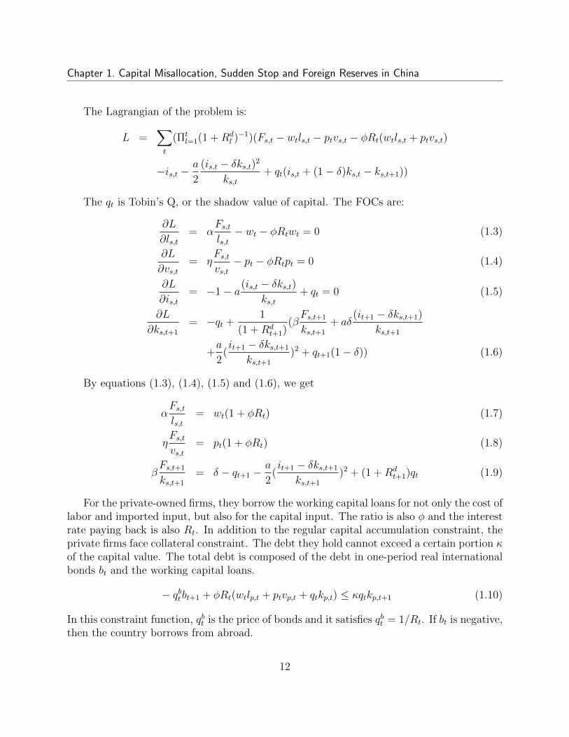
The Lagrangian of the problem is:
L =∑t
(Πtl=1(1 +Rd
l )−1)(Fs,t − wtls,t − ptvs,t − φRt(wtls,t + ptvs,t)
−is,t −a
2
(is,t − δks,t)2
ks,t+ qt(is,t + (1− δ)ks,t − ks,t+1))
The qt is Tobin’s Q, or the shadow value of capital. The FOCs are:
∂L
∂ls,t= α
Fs,tls,t− wt − φRtwt = 0 (1.3)
∂L
∂vs,t= η
Fs,tvs,t− pt − φRtpt = 0 (1.4)
∂L
∂is,t= −1− a(is,t − δks,t)
ks,t+ qt = 0 (1.5)
∂L
∂ks,t+1
= −qt +1
(1 +Rdt+1)
(βFs,t+1
ks,t+1
+ aδ(it+1 − δks,t+1)
ks,t+1
+a
2(it+1 − δks,t+1
ks,t+1
)2 + qt+1(1− δ)) (1.6)
By equations (1.3), (1.4), (1.5) and (1.6), we get
αFs,tls,t
= wt(1 + φRt) (1.7)
ηFs,tvs,t
= pt(1 + φRt) (1.8)
βFs,t+1
ks,t+1
= δ − qt+1 −a
2(it+1 − δks,t+1
ks,t+1
)2 + (1 +Rdt+1)qt (1.9)
For the private-owned firms, they borrow the working capital loans for not only the cost oflabor and imported input, but also for the capital input. The ratio is also φ and the interestrate paying back is also Rt. In addition to the regular capital accumulation constraint, theprivate firms face collateral constraint. The debt they hold cannot exceed a certain portion κof the capital value. The total debt is composed of the debt in one-period real internationalbonds bt and the working capital loans.
− qbtbt+1 + φRt(wtlp,t + ptvp,t + qtkp,t) ≤ κqtkp,t+1 (1.10)
In this constraint function, qbt is the price of bonds and it satisfies qbt = 1/Rt. If bt is negative,then the country borrows from abroad.
12
Chapter 1. Capital Misallocation, Sudden Stop and Foreign Reserves in China
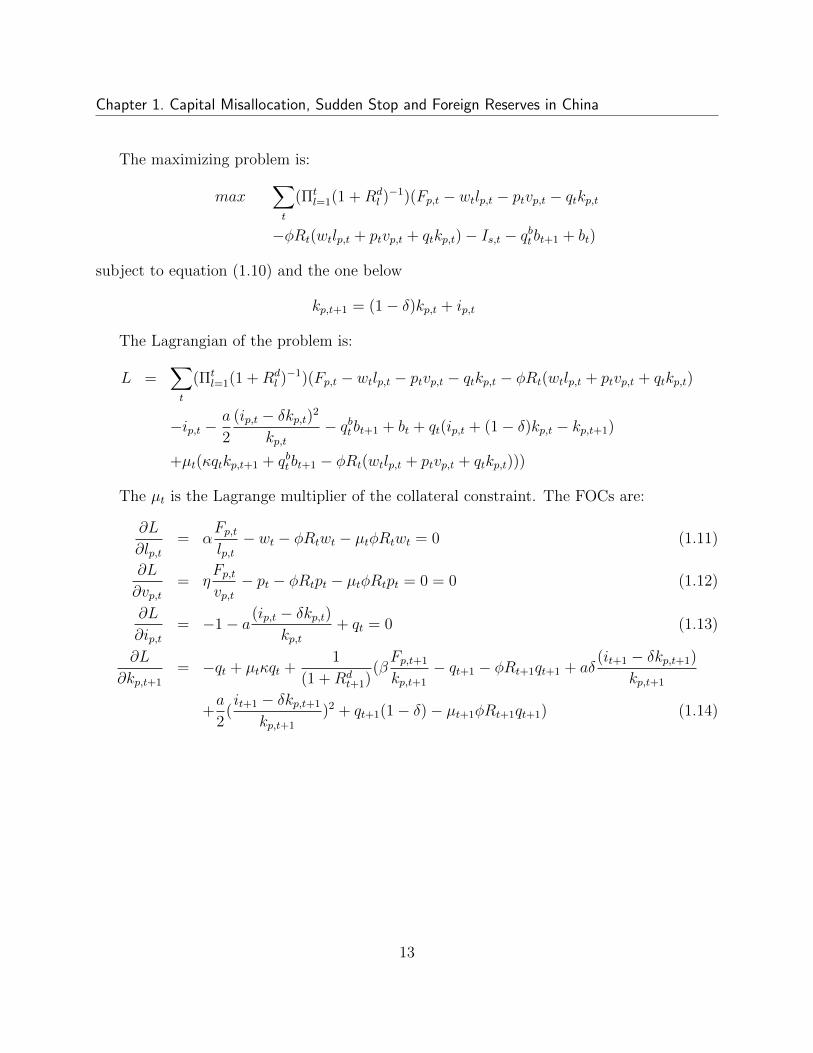
The maximizing problem is:
max∑t
(Πtl=1(1 +Rd
l )−1)(Fp,t − wtlp,t − ptvp,t − qtkp,t
−φRt(wtlp,t + ptvp,t + qtkp,t)− Is,t − qbtbt+1 + bt)
subject to equation (1.10) and the one below
kp,t+1 = (1− δ)kp,t + ip,t
The Lagrangian of the problem is:
L =∑t
(Πtl=1(1 +Rd
l )−1)(Fp,t − wtlp,t − ptvp,t − qtkp,t − φRt(wtlp,t + ptvp,t + qtkp,t)
−ip,t −a
2
(ip,t − δkp,t)2
kp,t− qbtbt+1 + bt + qt(ip,t + (1− δ)kp,t − kp,t+1)
+µt(κqtkp,t+1 + qbtbt+1 − φRt(wtlp,t + ptvp,t + qtkp,t)))
The µt is the Lagrange multiplier of the collateral constraint. The FOCs are:
∂L
∂lp,t= α
Fp,tlp,t− wt − φRtwt − µtφRtwt = 0 (1.11)
∂L
∂vp,t= η
Fp,tvp,t− pt − φRtpt − µtφRtpt = 0 = 0 (1.12)
∂L
∂ip,t= −1− a(ip,t − δkp,t)
kp,t+ qt = 0 (1.13)
∂L
∂kp,t+1
= −qt + µtκqt +1
(1 +Rdt+1)
(βFp,t+1
kp,t+1
− qt+1 − φRt+1qt+1 + aδ(it+1 − δkp,t+1)
kp,t+1
+a
2(it+1 − δkp,t+1
kp,t+1
)2 + qt+1(1− δ)− µt+1φRt+1qt+1) (1.14)
13
Chapter 1. Capital Misallocation, Sudden Stop and Foreign Reserves in China
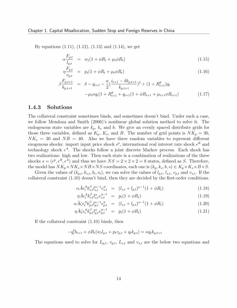
By equations (1.11), (1.12), (1.13) and (1.14), we get
αFp,tlp,t
= wt(1 + φRt + µtφRt) (1.15)
ηFp,tvp,t
= pt(1 + φRt + µtφRt) (1.16)
βFp,t+1
kp,t+1
= δ − qt+1 −a
2(it+1 − δkp,t+1
kp,t+1
)2 + (1 +Rdt+1)qt
−µtκqt(1 +Rdt+1 + qt+1(1 + φRt+1 + µt+1φRt+1) (1.17)
1.4.3 Solutions
The collateral constraint sometimes binds, and sometimes doesn’t bind. Under such a case,we follow Mendoza and Smith (2006)’s nonlinear global solution method to solve it. Theendogenous state variables are kp, ks and b. We give an evenly spaced distribute grids forthose three variables, defined as Kp, Ks, and B. The number of grid points is NKp = 30,NKs = 30 and NB = 40. Also we have three random variables to represent differentexogenous shocks: import input price shock εp, international real interest rate shock εR andtechnology shock εA. The shocks follow a joint discrete Markov process. Each shock hastwo realizations: high and low. Then each state is a combination of realizations of the threeshocks s = (εp, εR, εA) and thus we have NS = 2× 2× 2 = 8 states, defined as S. Therefore,the model has NKp×NKs×NB×NS coordinates, each one is (kp, ks, b, s) ∈ Kp×Ks×B×S.
Given the values of (kp,t, ks,t, bt, st), we can solve the values of lp,t, ls,t, vp,t and vs,t. If thecollateral constraint (1.10) doesn’t bind, then they are decided by the first-order conditions.
αAεAt kβs,tl
α−1s,t v
ηs,t = (ls,t + lp,t)
ω−1(1 + φRt) (1.18)
ηAεAt kβs,tl
αs,tv
η−1s,t = pt(1 + φRt) (1.19)
αAζεAt kβp,tl
α−1p,t v
ηp,t = (ls,t + lp,t)
ω−1(1 + φRt) (1.20)
ηAζεAt kβp,tl
αp,tv
η−1p,t = pt(1 + φRt) (1.21)
If the collateral constraint (1.10) binds, then
−qbtbt+1 + φRt(wtlp,t + ptvp,t + qtkp,t) = κqtkp,t+1
The equations used to solve for Lp,t, vp,t, Ls,t and vs,t are the below two equations and
14
Chapter 1. Capital Misallocation, Sudden Stop and Foreign Reserves in China
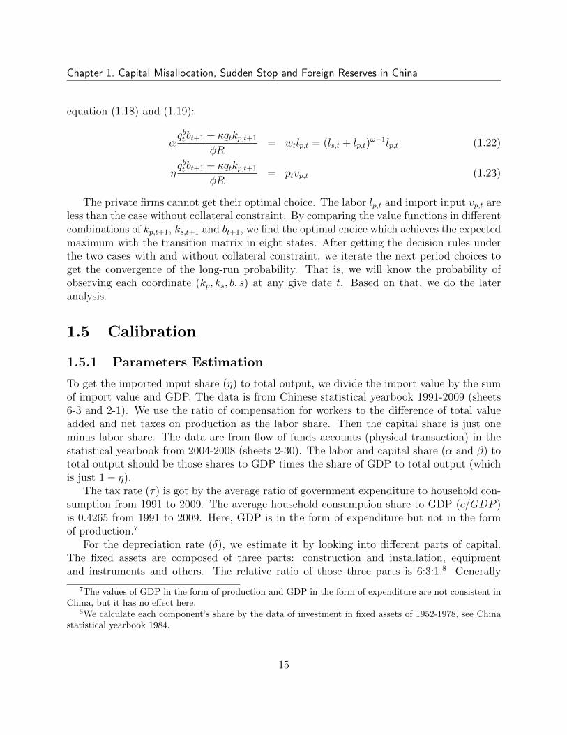
equation (1.18) and (1.19):
αqbtbt+1 + κqtkp,t+1
φR= wtlp,t = (ls,t + lp,t)
ω−1lp,t (1.22)
ηqbtbt+1 + κqtkp,t+1
φR= ptvp,t (1.23)
The private firms cannot get their optimal choice. The labor lp,t and import input vp,t areless than the case without collateral constraint. By comparing the value functions in differentcombinations of kp,t+1, ks,t+1 and bt+1, we find the optimal choice which achieves the expectedmaximum with the transition matrix in eight states. After getting the decision rules underthe two cases with and without collateral constraint, we iterate the next period choices toget the convergence of the long-run probability. That is, we will know the probability ofobserving each coordinate (kp, ks, b, s) at any give date t. Based on that, we do the lateranalysis.
1.5 Calibration
1.5.1 Parameters Estimation
To get the imported input share (η) to total output, we divide the import value by the sumof import value and GDP. The data is from Chinese statistical yearbook 1991-2009 (sheets6-3 and 2-1). We use the ratio of compensation for workers to the difference of total valueadded and net taxes on production as the labor share. Then the capital share is just oneminus labor share. The data are from flow of funds accounts (physical transaction) in thestatistical yearbook from 2004-2008 (sheets 2-30). The labor and capital share (α and β) tototal output should be those shares to GDP times the share of GDP to total output (whichis just 1− η).
The tax rate (τ) is got by the average ratio of government expenditure to household con-sumption from 1991 to 2009. The average household consumption share to GDP (c/GDP )is 0.4265 from 1991 to 2009. Here, GDP is in the form of expenditure but not in the formof production.7
For the depreciation rate (δ), we estimate it by looking into different parts of capital.The fixed assets are composed of three parts: construction and installation, equipmentand instruments and others. The relative ratio of those three parts is 6:3:1.8 Generally
7The values of GDP in the form of production and GDP in the form of expenditure are not consistent inChina, but it has no effect here.
8We calculate each component’s share by the data of investment in fixed assets of 1952-1978, see Chinastatistical yearbook 1984.
15
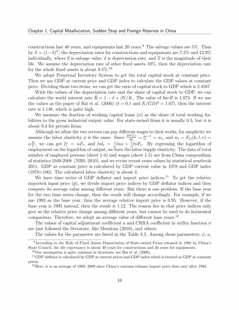
Chapter 1. Capital Misallocation, Sudden Stop and Foreign Reserves in China
constructions last 40 years, and equipments last 20 years.9 The salvage values are 5%. Thusby S = (1−δ)T , the depreciation rates for constructions and equipments are 7.2% and 13.9%individually, where S is salvage value, δ is depreciation rate, and T is the magnitude of theirlife. We assume the depreciation rate of other fixed assets 10%, then the depreciation ratefor the whole fixed assets is about 9.5%.10
We adopt Perpetual Inventory System to get the total capital stock at constant price.Then we use GDP at current price and GDP index to calculate the GDP values at constantprice. Dividing those two items, we can get the ratio of capital stock to GDP which is 2.4587.
With the values of the depreciation rate and the share of capital stock to GDP, we cancalculate the world interest rate R = 1 − δ + βY/K. The value of barR is 1.073. If we usethe values as the paper of Bai et al. (2006) (δ = 0.1 and K/GDP = 1.67), then the interestrate is 1.148, which is quite high.
We measure the fraction of working capital loans (φ) as the share of total working lia-bilities to the gross industrial output value. For state-owned firms it is usually 0.5, but it isabout 0.3 for private firms.
Although we allow the two sectors can pay different wages to their works, for simplicity weassume the labor elasticity φ is the same. Since ∂N(lt)
∂lt= lω−1
t = wt, and wt = Fl,t(k, l, v) =
αFtlt
, we can get lωt = αFt, and lnlt = 1ωlnα + 1
ωlnFt. By regressing the logarithm of
employment on the logarithm of output, we have the labor supply elasticity. The data of totalnumber of employed persons (sheet 1-4) and wages (sheet 1-5) are from China compendiumof statistics 1949-2008 (NBS, 2010), and we revise recent years values by statistical yearbook2011. GDP at constant price is calculated by GDP current value in 1978 and GDP index(1978=100). The calculated labor elasticity is about 4.
We have time series of GDP deflator and import price indices.11 To get the relativeimported input price (p), we divide import price indices by GDP deflator indices and thencompute its average value among different years. But there is one problem. If the base yearfor the two time series change, then the result will change accordingly. For example, if weuse 1993 as the base year, then the average relative import price is 0.95. However, if thebase year is 1995 instead, then the result is 1.12. The reason lies in that price indices onlygive us the relative price change among different years, but cannot be used to do horizontalcomparison. Therefore, we adopt an average value of different base years.12
The values of capital adjustment coefficient a and CRRA coefficient in utility function σare just followed the literature, like Mendoza (2010), and others.
The values for the parameter are listed in the Table 3.3. Among those parameters, φ, a,
9According to the Rule of Fixed Assets Depreciation of State-owned Firms released in 1985 by China’sState Council, the life expectancy is about 40 years for constructions and 20 years for equipments.
10Our assumption is quite common in literature, see Bai et al. (2006).11GDP deflator is calculated by GDP at current prices and GDP index which is treated as GDP at constant
prices.12Here, it is an average of 1993- 2009 since China’s customs releases import price data only after 1993.
16
Chapter 1. Capital Misallocation, Sudden Stop and Foreign Reserves in China
σ can be used to do parameters robust check. A and ζ are adjusted to simulate the modelto the real China’s economy.
1.5.2 Shocks and Estimation
The shocks are from import input price, real international interest rate and productivity.We let the positive and negative shocks are both one standard deviation from the steadystate level.13
To calibrate the transition matrix, we also need to get the first order autocorrelationsand correlations among shocks for the above three variables. Price indices of imported goodsare released by General Administration of Customs of the People’s Republic of China. Thereare two types of import price index. One is the index over the same period of the previousyear, and the other is the one which sets last year average 100. Based on those two series wecan calculate the import price index which uses the average of a certain year as base (100).Here we use the year 2004 as the base year. As one of the tools to implement monetarypolicies, the interest rate is controlled by the People’s Bank of China (PBoC). The officialinterest rates of deposits and loans of financial institutions doesn’t fluctuate frequently andthey are only adjusted when the central bank decides to use monetary policy to managemoney flow or just send a signal to the market. Here we find the data of official interestrates of deposits of financial institutions (1 year) and the date when it was adjusted in themonetary policy department of PBoC. We use the yearly average deposit interest rate levelas nominal interest rate. Then it is deflated by GDP deflator to get the real interest rate.We use the common methods to decompose the GDP growth rate and calculate the TotalFactor Productivity (TFP).14 We find the correlations among the three variables are small(the absolute value less than 0.12), thus we assume the shocks are independent. Table 1.5list their standard deviations and first order correlations.
1.6 Results
1.6.1 Long Run Moments of Major Variables
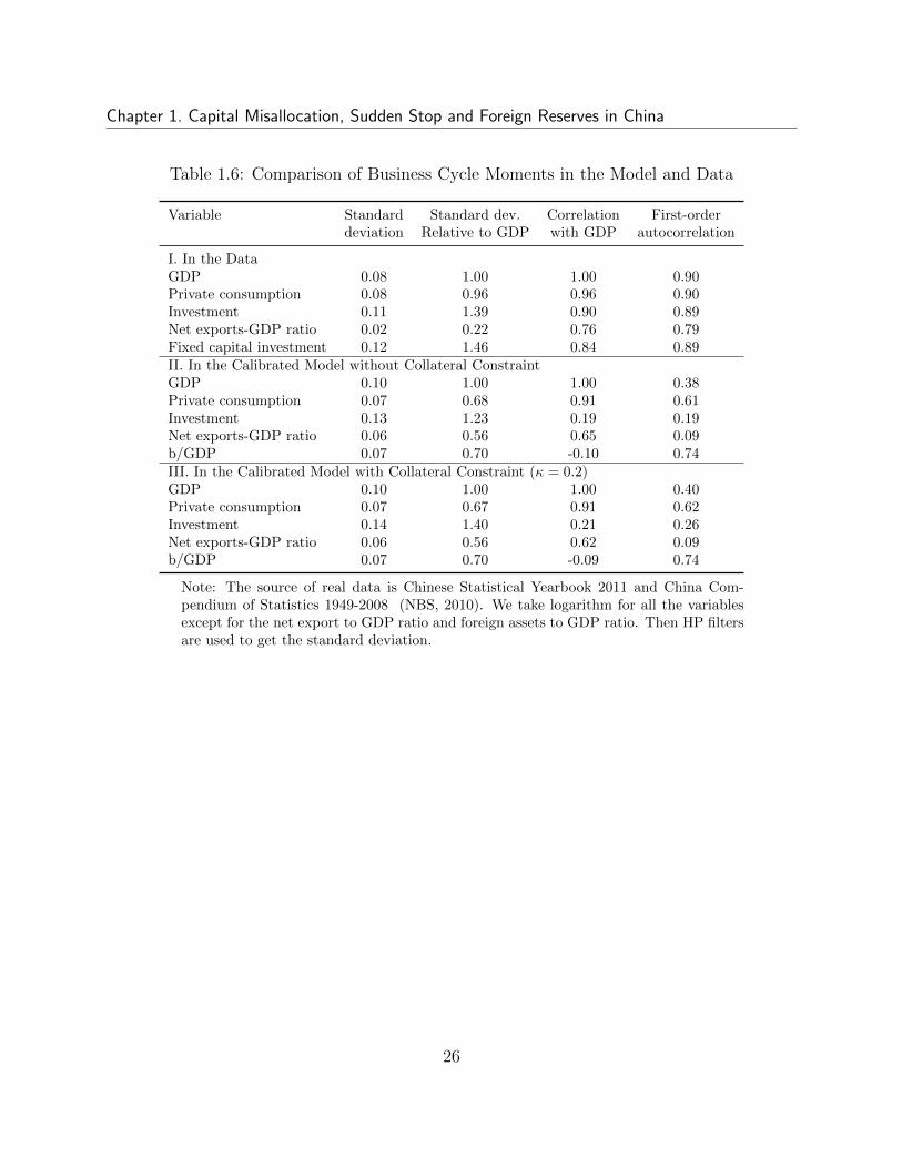
First, let’s look at the performance of our model under two cases: without and with collateralconstraint. No matter under which cases, they can match the long-run business cyclesmoments pretty well, which is also the result of the paper Mendoza (2010). Table 1.6shows the moments for the major economic variables, including GDP, private consumption,investment, net export to GDP ratio and foreign assets to GDP ratio in the real data and
13The real interest rate is too volatile, and thus we only apply one tenth of its standard deviation.14The source of data of GDP at constant price, labor, capital stock and shares of capital and labor are
the same as previously mentioned.
17
Chapter 1. Capital Misallocation, Sudden Stop and Foreign Reserves in China
calibrated models. The real data is from Chinese Statistical Yearbook 2011 and ChinaCompendium of Statistics 1949-2008 (NBS, 2010). The moments here include standarddeviation (in percent), standard deviation relative to GDP, correlation with GDP and first-order autocorrelation. In the real data, private consumption is less volatile than GDP andinvestment is more volatile. The consumption, investment and next exports to GDP ratioall correlated with GDP tightly. But the net export is not counter-cyclical like the analysisin Mendoza (2010). By several countries evidence, Backus and Kehoe (1992) show thatin two-thirds of the cases, the correlation with GDP is negative, and in the other cases,the correlation is generally small. Thus the pro-cyclicity of net export in China is not aspecial thing. In the calibrated models, there is no big difference between the one withoutcollateral constraint and the one with it. They both display the same moments as theempirical evidence. Only for the first-order autocorrelation, the calibrated models havesmaller magnitude.
1.6.2 Sudden Stop Event Simulation
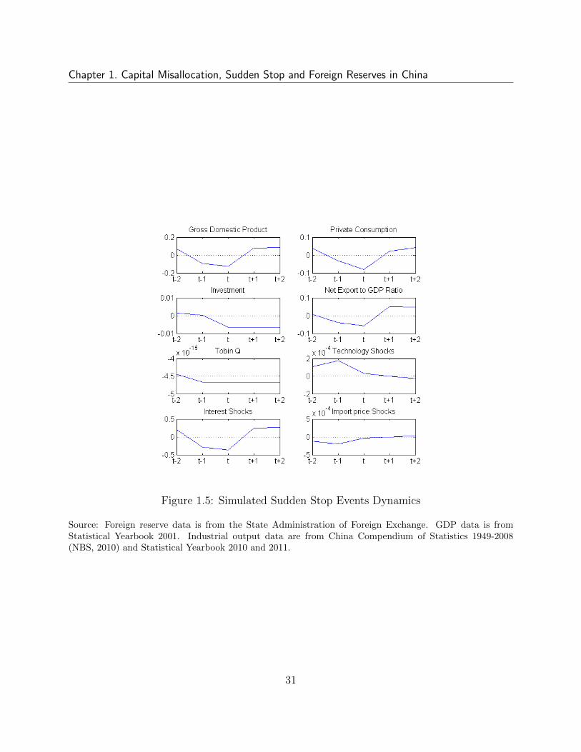
In literature, three main empirical regularities define sudden stop: reversals of internationalcapital flows, reflected in sudden increases in net exports and the current account; declines inproduction and absorption; and corrections in asset prices. Mendoza (2010) and Calvo et al.(2006) use net exports-GDP ratio as 2 percentage points above the mean as the definitionof sudden stop states. However, this criterion seems to be not feasible for the case of Chinagiven the fact that China’s export/GDP ratio increased significantly. Meanwhile, there isno sudden stop event in the past three decades which demonstrates the above three featuresat the same time in China. China also has current account surplus since 1994, and thesurplus is more than 200 billion U.S. dollars in 2011. Thus, it already has significant capitaloutflow. Thus, in the sense of reversals from capital inflow to outflow, it is unlikely to havesudden stop in China. But it doesn’t mean we have no need to worry about. China’s outputhas experienced fast growth in the past thirty years. We all care about its prospect. If ithas a dramatic decline, then clearly it will cause many other problems like unemployment,stock market crash and even social instability. Therefore we want to predict the behaviors ofother variables when the output declines significantly. Thus in the case of China, we definesudden stop states as those in which the collateral constraint binds with positive long-runprobability and the GDP is at least 2 percentage points below its mean.
To see the dynamics of the simulated sudden stop event, we conduct a 10,000 time periodsstochastic simulation and then construct a five-year event windows around the sudden stopevent.15 Figure 1.5 shows the dynamics for GDP, private consumption, investment, netexports to GDP ratio, Tobin Q and the three exogenous variables (technology, internationalinterest and import price). For the first four variables, we take logarithm. Then HP filters
15The calibrated parameters are based on the yearly data, thus here the time periods are represented byyears.
18

Chapter 1. Capital Misallocation, Sudden Stop and Foreign Reserves in China
are used to get the deviations from the trends. Among the simulated 10,000 time series, weidentify the sudden stop events as the situation in which the collateral constraint binds andGDP is at least one standard deviation below the trend. Unlike the papers in Mendoza (2010)and Calvo et al. (2006), we don’t use the net export to GDP ratio (at least one standarddeviation above trend) as an identification because China’s real situations are quite differentfrom Mexico as we explain in the above paragraph. We depict the median deviation fromthe trend for each variable around the sudden stop event.
The model predicts that two periods before Sudden Stops GDP and private consumptionbegin to decline and after that they increase quickly. On the second periods before andafter sudden stop, output and consumption are above the trend. But for the investmentalthough it is above trend before the sudden stop event, it cannot recover after two periods.Net export to GDP ratio has the same dynamics as output and consumption. It is stillpro-cyclical which is far different from other capital inflow countries. The Tobin’s Q’s pathalso has no recovery which might not be a good implication of the calibrated model.
1.6.3 Effects of Relative Productivity
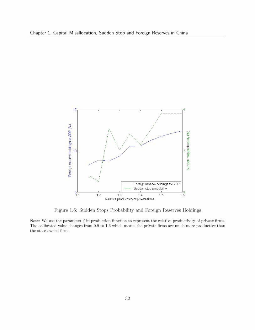
In order to simulate the high growth path in China, we have two choices: increase A orζ. The increase of A means there is technology improvement in both two sectors, but therelative efficiency doesn’t change. The increase of ζ means there is an improvement inrelative productivity of the private firms and the technology level of the state-owned firmskeeps constant. The combination of these two parameters change is more suitable to the realeconomy path. But here we want to show the effect of relative productivity. If the parameterζ increases from 0.9 to 1.6, then the output share of private firms changes from 42% to 73%.It is close to the development path of Chinese private firms in the past two decades (seeFigure 1.1). With the increase of productivity of private firms, the corresponding SuddenStops probability and the international bonds holding both increase (Figure 1.6).
By Figure 1.7, we are confirmed that higher productivity will lead to bigger shares in thetotal output. Currently the private firms contribute about 70% to the whole production (year2010). In our calibrated model it links to the productivity coefficient ζ = 1.5. We depictit as a point in Figure 1.7. Also by that figure we can tell higher output share is positivelyrelated to the foreign reserve holdings and Sudden Stops probability. Corresponding to theprivate firms’ share, the ratio of foreign reserve holdings to GDP would be 12.4% in 2010. Inreality there were 2,847 billion U.S. dollars reserves in China in 2010 and it was 48% of GDP.Our calibration result can explain a quarter of the foreign reserves accumulation. For theunexplained part, the reason may lay in the governments’ behavior. Figure 1.8 shows thatsavings of general governments are more than 40 percent of the total domestic savings from1992 to 2008. And in some years it exceeds 50 percent. Thus government’s behavior playsan important role in explaining foreign reserves. In the future work, it would be helpful toinclude government into our model.
19

Chapter 1. Capital Misallocation, Sudden Stop and Foreign Reserves in China
1.6.4 Effects of Financial Development
To see the effect of financial improvement, we increase the value of κ. κ is the ratio of firms’maximum debt holding to its total capital wealth. Thus when it increases, it means the col-lateral constraint for the private firms loosens. Figure 1.9 shows with the decreasing financialconstraint or better financial environment, the ratio of sudden stop probability and foreignreserve holdings to GDP decrease too. It confirms our hypothesis that financial constraintis one of the reasons that private firms hold foreign reserves. With the improvement in fi-nancial restrictions, private firms can get the loans easily from domestic lenders, the capitalallocation will be more efficient and the precautionary saving part of firms will decrease.
1.7 Conclusions
In this paper we discuss the puzzle that China has very large growth rates and huge mag-nitude of foreign reserves accumulation. We use a two-sector DSGE model to explain theprivate firms’ incentive of precautionary savings. Then by calibration the major parame-ters from Chinese real data, we simulate the model and get some useful results. As therelative productivity of private firms to state-owned firms increases, the private firms’ sharein total output rises. They become the driving force of economic growth. And given thatprivate firms have collateral constraint and capital allocation is less efficient, the probabilityof Sudden Stops increases and foreign reserves holding increases too. In the real case ofChina’s macro economy the private firms contribute about 70% of industry output.16 Usingthe calibrated value of relative productivity of private firms corresponding to their outputshare, the Sudden Stops probability is 3.8%, and the share of foreign reserves holdings toGDP is 12.4%. Our model can explain about 25% of China’s reserves holding. To interpretsuch a result, one way is that there must be other reasons that contribute a lot to such ahuge amount of foreign reserves and the other one is that China’s reserves holding is quiteexcessive.
In our model, we let the relative price of import to output is an exogenous shock. Butgiven China is a big country in terms of total output and trade volume, the import andexport price will be changed accordingly by China’s import and export volume. Thus asmall open economy hypothesis may need to be revised to fit China’s real case.
16Here it is only the industry output, and it doesn’t include other sectors.
20

Chapter 1. Capital Misallocation, Sudden Stop and Foreign Reserves in China
Tab
le1.
1:C
hin
a’s
Exte
rnal
Deb
t,20
01-2
011
Yea
r20
012002
2003
2004
2005
2006
2007
2008
2009
2010
2011
Tot
alIn
bil
lion
sof
U.S
.d
olla
rs20
3.3
202.6
219.4
263.0
296.5
338.6
389.2
390.2
428.6
548.9
695.0
In%
ofG
DP
15.3
13.9
13.4
13.6
13.1
12.5
11.1
8.6
8.6
9.3
9.5
In%
ofex
por
tof
good
san
dse
rvic
e67
.955.5
45.2
40.1
35.4
31.9
29.0
24.7
32.1
31.3
30.3
In%
ofor
din
ary
exp
ort
171.0
139.1
111.6
99.1
85.8
73.8
64.8
51.8
69.9
65.7
65.5
By
mat
uri
ty(i
n%
ofto
tal
deb
t)S
hor
tte
rm41
.243.0
46.9
52.7
57.9
58.8
60.6
58.0
60.5
68.4
72.1
Med
ian
and
Lon
gte
rm58
.857.0
53.2
47.3
42.1
41.2
39.5
42.0
39.5
31.6
27.9
By
typ
e(i
n%
ofto
tal
deb
t)T
rad
eC
red
its
27.0
28.4
28.4
30.8
35.8
35.3
38.2
33.2
37.7
38.5
35.9
Reg
iste
red
exte
rnal
deb
t73
.071.6
71.6
69.2
64.2
64.7
61.8
66.8
62.3
61.5
64.1
Reg
iste
red
exte
rnal
deb
tby
deb
tor
(in
%of
tota
ld
ebt)
Min
istr
ies
un
der
the
Sta
teC
oun
cil
24.5
24.9
24.1
12.8
11.1
10.1
9.0
8.5
8.6
7.1
5.4
Ch
ines
e-fu
nd
edF
inan
cial
Inst
itu
tion
s16
.917.9
17.2
25.1
20.6
20.8
20.6
21.2
21.9
24.7
30.5
For
eign
-fu
nded
Fin
anci
alIn
stit
uti
ons
8.4
7.4
9.5
12.0
13.8
14.7
11.9
11.2
8.9
8.8
7.8
For
eign
-fu
nded
Ente
rpri
ses
17.3
16.4
17.2
17.0
17.0
18.0
19.0
24.6
21.7
20.0
19.6
Ch
ines
e-fu
nd
edE
nte
rpri
ses
5.5
4.9
3.5
2.3
1.5
1.0
1.2
1.1
1.0
1.1
0.9
Oth
ers
0.4
0.0
0.1
0.1
0.1
0.1
0.1
0.1
0.1
0.0
0.0
Sou
rce:
Ch
ina
Sta
teA
dm
inis
trat
ion
ofF
ore
ign
Exch
an
ge
an
dau
thor’
sca
lcu
lati
on
.T
he
trad
ecr
edit
isfr
om
surv
eyd
ata
,so
itm
ayn
otm
atch
wit
hth
etr
ade
cred
itin
the
Bala
nce
of
Pay
men
t.
21
Chapter 1. Capital Misallocation, Sudden Stop and Foreign Reserves in China
Table 1.2: Structure of China International Investment Position
Year 2004 2005 2006 2007 2008 2009 2010 2011
Net Asset (Billion $) 276 408 640 1188 1494 1491 1688 1775Asset (Billion $) 929 1223 1690 2416 2957 3437 4119 4718
Direct Investment Abroad (%) 5.7 5.3 5.4 4.8 6.3 7.2 7.7 7.7Portfolio Investments (%) 9.9 9.5 15.7 11.8 8.5 7.1 6.2 5.5Other Investments (%) 17.8 17.7 15.0 19.4 18.7 14.4 15.3 17.8Reserve Asset (%) 66.6 67.5 63.9 64.0 66.5 71.4 70.8 69.0
Liability (Billion $) 653 816 1050 1228 1463 1946 2431 2943Direct Investment in China (%) 56.5 57.8 58.5 57.3 62.6 67.5 64.6 61.3Portfolio Investments (%) 8.7 9.4 11.5 11.9 11.5 9.8 9.2 8.4Other Investments (%) 34.8 32.8 30.0 30.8 25.9 22.7 26.2 30.3
Source: China State Administration of Foreign Exchange and author’s calculation.
22
Chapter 1. Capital Misallocation, Sudden Stop and Foreign Reserves in China
Tab
le1.
3:C
hin
ese
Hol
din
gsof
U.S
.Sec
uri
ties
Yea
r20
0220
032004
2005
2006
2007
2008
2009
2010
2011
Tot
al18
1.5
255.
5341.0
527.3
698.9
922.0
1205.1
1464.0
1610.7
1726.6
Equity
4.0
1.9
2.5
2.5
3.8
28.5
99.5
77.7
126.5
158.8
Long-term
debt
164.
725
0.1
320.3
485.0
677.9
870.5
1075.3
1226.4
1479.3
1562.9
Short-term
debt
12.7
3.5
18.2
39.7
17.2
23.0
30.3
159.9
4.9
4.9
Ch
ina
fore
ign
rese
rve
286.
440
3.3
609.9
818.9
1066.3
1528.2
1946.0
2399.2
2847.3
3181.1
Sh
are
ofU
Sse
curi
ties
(%)
63.4
63.4
55.9
64.4
65.5
60.3
61.9
61.0
56.6
54.3
Sou
rce:
U.S
.D
epar
tmen
tof
the
Tre
asu
ryan
dau
thor’
sca
lcu
lati
on
.
23
Chapter 1. Capital Misallocation, Sudden Stop and Foreign Reserves in China
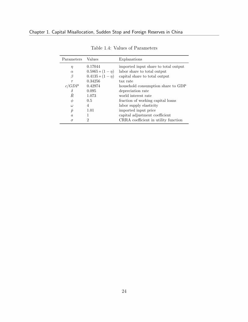
Table 1.4: Values of Parameters
Parameters Values Explanations
η 0.17044 imported input share to total outputα 0.5865 ∗ (1− η) labor share to total outputβ 0.4135 ∗ (1− η) capital share to total outputτ 0.34256 tax rate
c/GDP 0.42974 household consumption share to GDPδ 0.095 depreciation rateR 1.073 world interest rateφ 0.5 fraction of working capital loansω 4 labor supply elasticityp 1.01 imported input pricea 1 capital adjustment coefficientσ 2 CRRA coefficient in utility function
24
Chapter 1. Capital Misallocation, Sudden Stop and Foreign Reserves in China
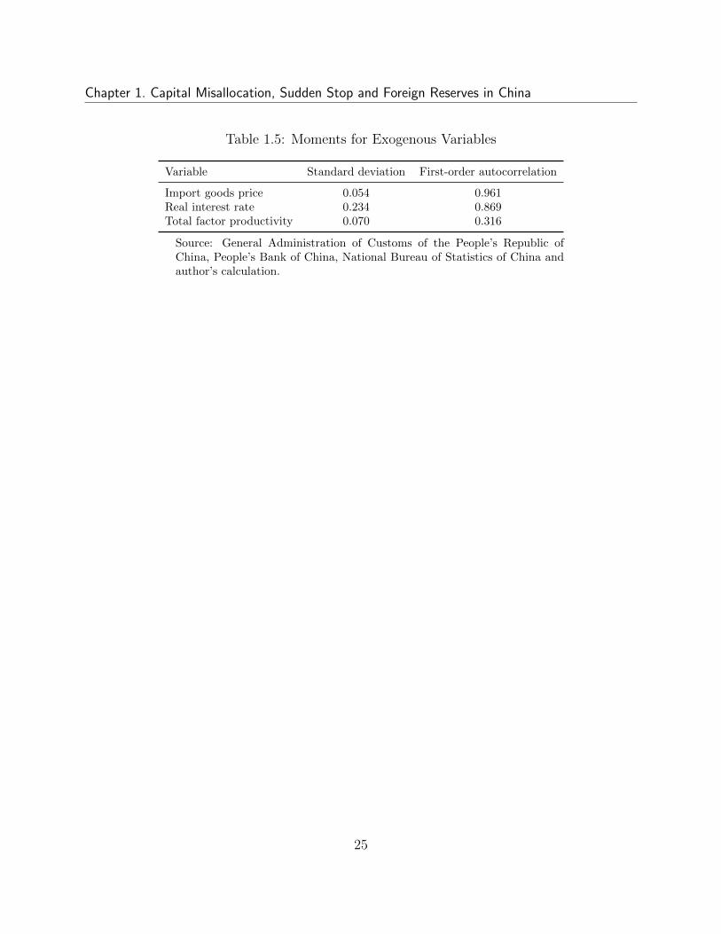
Table 1.5: Moments for Exogenous Variables
Variable Standard deviation First-order autocorrelation
Import goods price 0.054 0.961Real interest rate 0.234 0.869Total factor productivity 0.070 0.316
Source: General Administration of Customs of the People’s Republic ofChina, People’s Bank of China, National Bureau of Statistics of China andauthor’s calculation.
25
Chapter 1. Capital Misallocation, Sudden Stop and Foreign Reserves in China
Table 1.6: Comparison of Business Cycle Moments in the Model and Data
Variable Standarddeviation
Standard dev.Relative to GDP
Correlationwith GDP
First-orderautocorrelation
I. In the DataGDP 0.08 1.00 1.00 0.90Private consumption 0.08 0.96 0.96 0.90Investment 0.11 1.39 0.90 0.89Net exports-GDP ratio 0.02 0.22 0.76 0.79Fixed capital investment 0.12 1.46 0.84 0.89II. In the Calibrated Model without Collateral ConstraintGDP 0.10 1.00 1.00 0.38Private consumption 0.07 0.68 0.91 0.61Investment 0.13 1.23 0.19 0.19Net exports-GDP ratio 0.06 0.56 0.65 0.09b/GDP 0.07 0.70 -0.10 0.74III. In the Calibrated Model with Collateral Constraint (κ = 0.2)GDP 0.10 1.00 1.00 0.40Private consumption 0.07 0.67 0.91 0.62Investment 0.14 1.40 0.21 0.26Net exports-GDP ratio 0.06 0.56 0.62 0.09b/GDP 0.07 0.70 -0.09 0.74
Note: The source of real data is Chinese Statistical Yearbook 2011 and China Com-pendium of Statistics 1949-2008 (NBS, 2010). We take logarithm for all the variablesexcept for the net export to GDP ratio and foreign assets to GDP ratio. Then HP filtersare used to get the standard deviation.
26
Chapter 1. Capital Misallocation, Sudden Stop and Foreign Reserves in China
Figure 1.1: Foreign Reserves Ratio to GDP and Private Firms Output Share in China (1980-2010)
Source: Foreign reserve data is from the State Administration of Foreign Exchange. GDP data is fromStatistical Yearbook 2001. Industrial output data are from China Compendium of Statistics 1949-2008(NBS, 2010) and Statistical Yearbook 2010 and 2011.
27
Chapter 1. Capital Misallocation, Sudden Stop and Foreign Reserves in China
Figure 1.2: Liabilities-to-Assets Ratio of Industrial Firms (2000)
Source: Chinese Annual Survey of Industrial Production 2000.Note: Groups are categorized by the size of firms’ assets. From Group 1 to Group 10, firms’ assets increase.
28
Chapter 1. Capital Misallocation, Sudden Stop and Foreign Reserves in China
Figure 1.3: External Debt in China (1985-2011)
Source: China State Administration of Foreign Exchange.
29
Chapter 1. Capital Misallocation, Sudden Stop and Foreign Reserves in China
Figure 1.4: The Compostion of Annual Capital Inflows in China 1982-2011 (%)
Source: China State Administration of Foreign Exchange and author’s calculation.
30
Chapter 1. Capital Misallocation, Sudden Stop and Foreign Reserves in China
Figure 1.5: Simulated Sudden Stop Events Dynamics
Source: Foreign reserve data is from the State Administration of Foreign Exchange. GDP data is fromStatistical Yearbook 2001. Industrial output data are from China Compendium of Statistics 1949-2008(NBS, 2010) and Statistical Yearbook 2010 and 2011.
31
Chapter 1. Capital Misallocation, Sudden Stop and Foreign Reserves in China
Figure 1.6: Sudden Stops Probability and Foreign Reserves Holdings
Note: We use the parameter ζ in production function to represent the relative productivity of private firms.The calibrated value changes from 0.9 to 1.6 which means the private firms are much more productive thanthe state-owned firms.
32
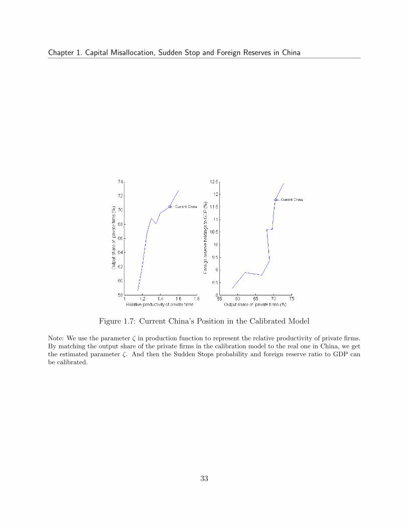
Chapter 1. Capital Misallocation, Sudden Stop and Foreign Reserves in China
Figure 1.7: Current China’s Position in the Calibrated Model
Note: We use the parameter ζ in production function to represent the relative productivity of private firms.By matching the output share of the private firms in the calibration model to the real one in China, we getthe estimated parameter ζ. And then the Sudden Stops probability and foreign reserve ratio to GDP canbe calibrated.
33
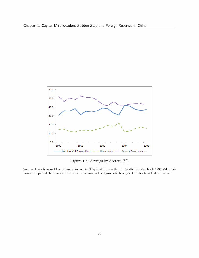
Chapter 1. Capital Misallocation, Sudden Stop and Foreign Reserves in China
Figure 1.8: Savings by Sectors (%)
Source: Data is from Flow of Funds Accounts (Physical Transaction) in Statistical Yearbook 1996-2011. Wehaven’t depicted the financial institutions’ saving in the figure which only attributes to 4% at the most.
34
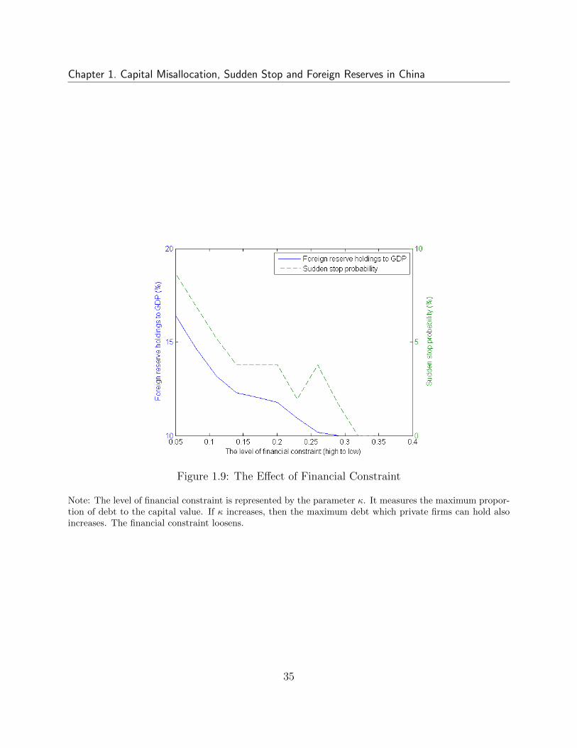
Chapter 1. Capital Misallocation, Sudden Stop and Foreign Reserves in China
Figure 1.9: The Effect of Financial Constraint
Note: The level of financial constraint is represented by the parameter κ. It measures the maximum propor-tion of debt to the capital value. If κ increases, then the maximum debt which private firms can hold alsoincreases. The financial constraint loosens.
35
Chapter 2
The Relative Volatility of Commodity
Prices: A Reappraisal1
2.1 Introduction
Are the international prices of primary commodities more volatile than those of manufacturedgoods? This question has important implications for macroeconomic and development poli-cies, and the conventional wisdom expressed in academic and policy circles is that they are.The policy literature is replete with prescriptions for economies to cope with the volatilityof commodity prices, ranging from prescribed investments in financial hedging instrumentssuch as commodity futures to fiscal stabilization rules to help reduce the pass through ofcommodity price volatility into domestic economies. A recent example is the World Bank’s4 billion dollar contribution to a joint fund launched in June 21, 2011 with J.P. Morganto help developing countries invest in commodity-price hedging instruments.2 In fact, theconcern over the impact of commodity price volatility on developing countries has also ledthe World Bank to argue that economic diversification away from commodities should be apriority for these countries even if this requires industrial policies. These policy prescriptionsand concerns are valid, regardless of the relative volatility of commodity prices. Such policiesare justified even if the prices of commodities are less volatile than those of manufacturedgoods, for example, because many developing countries tend to have highly concentratedexport baskets that are associated with volatile terms of trade and thus macroeconomic un-certainty, which itself can lead to social unrest (Bruckner and Ciccone (2010)). In addition,the volatility of some commodities linked to food staples can result even in social unrest (seeArezki and Bruckner (2011)).
Indeed, there are good reasons to expect that commodity prices are relatively volatile.
1This paper is coauthored with Rabah Arezki and Daniel Lederman.2World Bank, Press Release No:2011/559/EXT, Washington, DC.
36
Chapter 2. The Relative Volatility of Commodity Prices: A Reappraisal
One is that commodities, by definition, are goods that retain their qualities over time,which allows economic agents to use them as financial assets. This might be the case, forexample, of gold and other commodities whose prices tend to rise amidst global financialuncertainty. Caballero et al. (2008b), for example, argued that the volatility of commodityprices could be due to the lack of a global safe asset (besides the U.S. Treasury bills). Anearlier literature argued that commodity price volatility was fueled by stockpiling policies tosecure access to food or fuel during times of relative scarcity (Deaton and Laroque (1992)).These mechanisms add price volatility because of unavoidable asymmetric stockpiling rules;that is, the stockpile of commodities cannot be negative. Yet another potential explanationis the lumpiness of exploration investments in mining, which results in inelastic supply inthe short run (Deaton and Laroque (2003)). Finally, more traditional economic analysis ofthe effects of random demand shocks on homogeneous (i.e., commodities) and differentiatedgoods (i.e., manufactured products) also suggests that the resulting price volatility of thelatter would tend to be lower as producers of differentiated products could maximize profitsby reducing supply in response to negative demand shocks.
However, there are also good reasons to expect a higher volatility of differentiated man-ufactured goods. Product innovation and differentiation itself might contribute to pricevolatility by producing frequent shifts in residual demand for existing varieties. Indeed,the trade literature has acknowledged the wide dispersion in unit values of within narrowlydefined product categories in the United States import data at the 10-digit level of the Har-monized System (HS) (Schott (2004)). Also, the demand for differentiated products mightbe more unstable with respect to household and aggregate income shocks than that for basiccommodities. For instance, the demand for fuel and food might decline proportionately lessthan the demand for automobiles or electronics when incomes fall.
In spite of these contradictory predictions, there are few analyses that systematicallycompare the volatility of commodity and manufactured goods prices. An important excep-tion is the historical study by Jacks et al. (2011), who examined the volatility of domesticprices since 1700 in several countries; however, it covered only few commodities due to dataconstraints. In contrast, analyses of the evolution and volatility of the average price of bas-kets of commodities relative to the average price of a basket of manufactured goods-usuallythe manufacturing unit value index (MUV) constructed by the International Monetary Fund-are omnipresent in the literature and policy documents (e.g. Cashin and McDermott (2002);Calvo-Gonzalez et al. (2010)).
Figures 2.1 and 2.2 show the time series of aggregate price indices for various defini-tions of primary commodities. These series seem to corroborate the conventional wisdomas commodity prices appear to be more volatile than non-commodity prices. The presentpaper challenges this conventional wisdom by providing a new stylized fact on the relativevolatility of primary commodity prices using data from U.S. imports data at the 10-digitlevel of aggregation in the Harmonized System (HS) nomenclature.
This paper contributes to several strands of the literature. First, it contributes more
37
Chapter 2. The Relative Volatility of Commodity Prices: A Reappraisal
directly to the literature studying the behavior of commodity prices. This literature does notnecessarily compare commodity prices to non commodity prices but focuses on the former.For instance, Deaton and Laroque (1992) used coefficients of variation of aggregated priceindexes as a measure of volatility to analyze the volatility of 13 commodities. They arguethat “commodity prices are extremely volatile” but do not provide an explicit comparisonwith non-commodity price volatility.3 As far as we know, this paper is the first to comparethe volatility of individual primary commodity prices not with aggregate indexes but ratherwith disaggregated monthly data.
Second, our paper contributes to the literature on trends in commodity prices relativeto manufactured products (e.g., Harvey et al. (2010)). Our paper instead focuses on thedifferences in the second moments of commodity prices compared to those of non-commodityprices.
Third, this paper also contributes to the literature on the so-called “resource curse” thathas focused on the adverse effect of resource endowments on economic growth (e.g., Leder-man and Maloney (2007); Van der Ploeg (2011); Frankel (2010)). If commodity prices areintrinsically more volatile than the prices of manufactured goods, a higher natural resourceendowments could result in higher macroeconomic volatility.
The rest of this paper is organized as follows. Section 2.2 discusses the monthly datafrom the United States international trade records over the period from 2002 to 2011 coveringmore than 18 thousand goods. Section 2.3 presents the main results. Section 2.4 providesan array of robustness tests. Section 2.5 concludes.
2.2 Data
Our data come from trade records of the United States, classified at the 10-digit level ofthe Harmonized System (HS) of trade classification. We use monthly frequency import datafrom January 2002 to April 2011. The data was obtained from the Foreign Trade Divisionof the U.S. Census Bureau. From these data, prices were computed as the ratio of importvalues to quantities. These unit values are used as our proxy for goods prices.
In total, the dataset covers 26,459 product categories. However, not all categories haveprice information; 7,976 products do not. Also, the analysis of volatility requires data forextended periods of time, and we dropped products that do not have price data for at least36 consecutive months. The final data set thus covers 12,955 products.4 Our benchmark
3More recently, Deaton and Laroque (2003) have focused on the longer-run determinants of commodityprices. They developed a Lewis model where commodity supply is infinitely elastic in the long run and therate of growth of supply responds to the excess of the current price over the long-run supply price. They findthat commodity prices are stationary around its supply price and are driven in the short run by fluctuationsin world income.
4The results reported below are unaffected by alternative choices of datasets such as keeping productswith price data available throughout the whole sample period.
38
Chapter 2. The Relative Volatility of Commodity Prices: A Reappraisal
analysis focuses on U.S. imports data rather than on exports data for two reasons. First, thereporting of imports data is generally less subject to measurement errors than exports data,as imports are more subject to tariffs and inspections than exports. Second, U.S. importedproducts are more numerous and diverse than exports. In fact, the U.S. reports twice asmany imported as exported goods. Also, 17 percent of imports are commodities comparedto only 4 percent for exports. While studying the pattern of US exports may be relevant fora U.S. specific analysis, it is essential for our general analysis to use imports data.5
It is noteworthy that this sample period covers years of historically high volatility ofreal commodity prices, perhaps only surpassed by the early 1970s (see, e.g., Calvo-Gonzalezet al. (2010)). Consequently, if there is a period selection bias in the data, it would probablybias commodity price volatility upwards. But, again, such historical analyses focus on com-modity prices relative to an aggregate price index of non-commodity goods, which might bemisleading.
As a starting point, the analysis focuses on aggregate price indexes-see Figures 2.1 and2.2. A relevant issue in this type of analysis concerns the definition of commodities. TheInternational Monetary Fund has one such classification, which includes non-fuel, energyand all primary commodities. The United Nations Conference on Trade and Development(UNCTAD) also has a definition, which includes some commodities that are not in the IMF,such as cottonseed oil and manganese ore. Appendix A.1 lists the commodities includedunder both definitions. In addition, it is easy to tell which goods are manufactured in theNorth American Industry Classification System (NAICS). At the two digit level, chapters31-39 of the NAICS are classified as manufactured goods.
Since the data on import prices from the U.S. are classified according to the HarmonizedSystem, we used concordance tables between the HS and the NAICS.6 To match the HSdata classification to the IMF and UNCTAD commodity classifications, we used the namesof the commodities as keywords to find matching product descriptions in the trade data.
To assess the volatility of individual goods prices it is important to de-trend the priceseries. We report results based on the Hodrick-Prescott filtered series, but all results re-ported herein hold with alternative filters, including the Baxter-King band-pass filter andfirst differences.7 In all three cases, we measure volatility with the standard deviation of de-trended price series. After calculating the standard deviations for each 10-digit product, wecompare the distribution of volatilities across groups of goods, namely commodities versusmanufactured goods.
5Nevertheless, the main result presented in this paper holds when using US exports data rather thanimports.
6Robert Feenstra’s web site provides the concordance for data from 1989-2006:http://cid.econ.ucdavis.edu/. The U.S. Census Bureau provides concordance tables for 2010 and2011: http://www.cnesus.gov/foreign-trade/reference/codes/index.html.
7There is thus no concern that the main result presented in this paper is driven by the choice of filteringmethod.
39
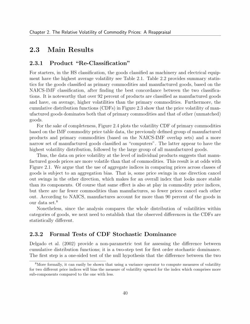
Chapter 2. The Relative Volatility of Commodity Prices: A Reappraisal
2.3 Main Results
2.3.1 Product “Re-Classification”
For starters, in the HS classification, the goods classified as machinery and electrical equip-ment have the highest average volatility see Table 2.1. Table 2.2 provides summary statis-tics for the goods classified as primary commodities and manufactured goods, based on theNAICS-IMF classification, after finding the best concordance between the two classifica-tions. It is noteworthy that over 92 percent of products are classified as manufactured goodsand have, on average, higher volatilities than the primary commodities. Furthermore, thecumulative distribution functions (CDFs) in Figure 2.3 show that the price volatility of man-ufactured goods dominates both that of primary commodities and that of other (unmatched)goods.
For the sake of completeness, Figure 2.4 plots the volatility CDF of primary commoditiesbased on the IMF commodity price table data, the previously defined group of manufacturedproducts and primary commodities (based on the NAICS-IMF overlap sets) and a morenarrow set of manufactured goods classified as “computers”. The latter appear to have thehighest volatility distribution, followed by the large group of all manufactured goods.
Thus, the data on price volatility at the level of individual products suggests that manu-factured goods prices are more volatile than that of commodities. This result is at odds withFigure 2.1. We argue that the use of aggregate indices in comparing prices across classes ofgoods is subject to an aggregation bias. That is, some price swings in one direction cancelout swings in the other direction, which makes for an overall index that looks more stablethan its components. Of course that same effect is also at play in commodity price indices,but there are far fewer commodities than manufactures, so fewer prices cancel each otherout. According to NAICS, manufactures account for more than 90 percent of the goods inour data set.8
Nonetheless, since the analysis compares the whole distribution of volatilities withincategories of goods, we next need to establish that the observed differences in the CDFs arestatistically different.
2.3.2 Formal Tests of CDF Stochastic Dominance
Delgado et al. (2002) provide a non-parametric test for assessing the difference betweencumulative distribution functions; it is a two-step test for first order stochastic dominance.The first step is a one-sided test of the null hypothesis that the difference between the two
8More formally, it can easily be shown that using a variance operator to compute measures of volatilityfor two different price indices will bias the measure of volatility upward for the index which comprises moresub-components compared to the one with less.
40
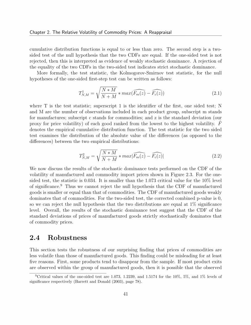
Chapter 2. The Relative Volatility of Commodity Prices: A Reappraisal
cumulative distribution functions is equal to or less than zero. The second step is a two-sided test of the null hypothesis that the two CDFs are equal. If the one-sided test is notrejected, then this is interpreted as evidence of weakly stochastic dominance. A rejection ofthe equality of the two CDFs in the two-sided test indicates strict stochastic dominance.
More formally, the test statistic, the Kolmogorov-Smirnov test statistic, for the nullhypotheses of the one-sided first-step test can be written as follows:
T 1N,M =
√N ∗MN +M
∗max(Fm(z)− Fc(z)) (2.1)
where T is the test statistic; superscript 1 is the identifier of the first, one sided test; Nand M are the number of observations included in each product group, subscript m standsfor manufactures; subscript c stands for commodities; and z is the standard deviation (ourproxy for price volatility) of each good ranked from the lowest to the highest volatility. Fdenotes the empirical cumulative distribution function. The test statistic for the two sidedtest examines the distribution of the absolute value of the differences (as opposed to thedifferences) between the two empirical distributions:
T 2N,M =
√N ∗MN +M
∗max|Fm(z)− Fc(z)| (2.2)
We now discuss the results of the stochastic dominance tests performed on the CDF of thevolatility of manufactured and commodity import prices shown in Figure 2.3. For the one-sided test, the statistic is 0.034. It is smaller than the 1.073 critical value for the 10% levelof significance.9 Thus we cannot reject the null hypothesis that the CDF of manufacturedgoods is smaller or equal than that of commodities. The CDF of manufactured goods weaklydominates that of commodities. For the two-sided test, the corrected combined p-value is 0,so we can reject the null hypothesis that the two distributions are equal at 1% significancelevel. Overall, the results of the stochastic dominance test suggest that the CDF of thestandard deviations of prices of manufactured goods strictly stochastically dominates thatof commodity prices.
2.4 Robustness
This section tests the robustness of our surprising finding that prices of commodities areless volatile than those of manufactured goods. This finding could be misleading for at leastfive reasons. First, some products tend to disappear from the sample. If most product exitsare observed within the group of manufactured goods, then it is possible that the observed
9Critical values of the one-sided test are 1.073, 1.2239, and 1.5174 for the 10%, 5%, and 1% levels ofsignificance respectively (Barrett and Donald (2003), page 78).
41
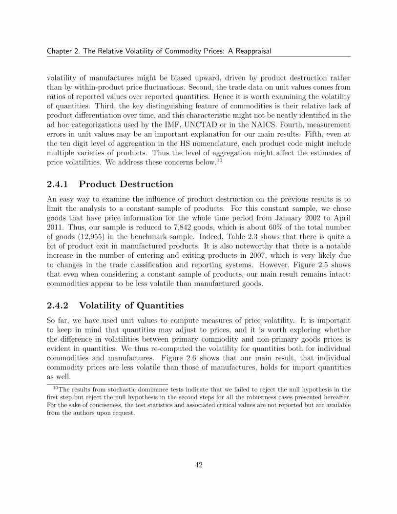
Chapter 2. The Relative Volatility of Commodity Prices: A Reappraisal
volatility of manufactures might be biased upward, driven by product destruction ratherthan by within-product price fluctuations. Second, the trade data on unit values comes fromratios of reported values over reported quantities. Hence it is worth examining the volatilityof quantities. Third, the key distinguishing feature of commodities is their relative lack ofproduct differentiation over time, and this characteristic might not be neatly identified in thead hoc categorizations used by the IMF, UNCTAD or in the NAICS. Fourth, measurementerrors in unit values may be an important explanation for our main results. Fifth, even atthe ten digit level of aggregation in the HS nomenclature, each product code might includemultiple varieties of products. Thus the level of aggregation might affect the estimates ofprice volatilities. We address these concerns below.10
2.4.1 Product Destruction
An easy way to examine the influence of product destruction on the previous results is tolimit the analysis to a constant sample of products. For this constant sample, we chosegoods that have price information for the whole time period from January 2002 to April2011. Thus, our sample is reduced to 7,842 goods, which is about 60% of the total numberof goods (12,955) in the benchmark sample. Indeed, Table 2.3 shows that there is quite abit of product exit in manufactured products. It is also noteworthy that there is a notableincrease in the number of entering and exiting products in 2007, which is very likely dueto changes in the trade classification and reporting systems. However, Figure 2.5 showsthat even when considering a constant sample of products, our main result remains intact:commodities appear to be less volatile than manufactured goods.
2.4.2 Volatility of Quantities
So far, we have used unit values to compute measures of price volatility. It is importantto keep in mind that quantities may adjust to prices, and it is worth exploring whetherthe difference in volatilities between primary commodity and non-primary goods prices isevident in quantities. We thus re-computed the volatility for quantities both for individualcommodities and manufactures. Figure 2.6 shows that our main result, that individualcommodity prices are less volatile than those of manufactures, holds for import quantitiesas well.
10The results from stochastic dominance tests indicate that we failed to reject the null hypothesis in thefirst step but reject the null hypothesis in the second steps for all the robustness cases presented hereafter.For the sake of conciseness, the test statistics and associated critical values are not reported but are availablefrom the authors upon request.
42
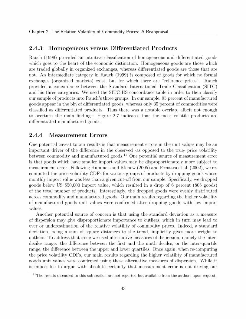
Chapter 2. The Relative Volatility of Commodity Prices: A Reappraisal
2.4.3 Homogeneous versus Differentiated Products
Rauch (1999) provided an intuitive classification of homogeneous and differentiated goodswhich goes to the heart of the economic distinction. Homogeneous goods are those whichare traded globally in organized exchanges, whereas differentiated goods are those that arenot. An intermediate category in Rauch (1999) is composed of goods for which no formalexchanges (organized markets) exist, but for which there are “reference prices”. Rauchprovided a concordance between the Standard International Trade Classification (SITC)and his three categories. We used the SITC-HS concordance table in order to then classifyour sample of products into Rauch’s three groups. In our sample, 95 percent of manufacturedgoods appear in the bin of differentiated goods, whereas only 35 percent of commodities wereclassified as differentiated products. Thus there was a notable overlap, albeit not enoughto overturn the main findings: Figure 2.7 indicates that the most volatile products aredifferentiated manufactured goods.
2.4.4 Measurement Errors
One potential caveat to our results is that measurement errors in the unit values may be animportant driver of the difference in the observed -as opposed to the true- price volatilitybetween commodity and manufactured goods.11 One potential source of measurement erroris that goods which have smaller import values may be disproportionately more subject tomeasurement error. Following Hummels and Klenow (2005) and Feenstra et al. (2002), we re-computed the price volatility CDFs for various groups of products by dropping goods whosemonthly import value was less than a given cut-off from our sample. Specifically, we droppedgoods below US $50,000 import value, which resulted in a drop of 6 percent (805 goods)of the total number of products. Interestingly, the dropped goods were evenly distributedacross commodity and manufactured goods. Our main results regarding the higher volatilityof manufactured goods unit values were confirmed after dropping goods with low importvalues.
Another potential source of concern is that using the standard deviation as a measureof dispersion may give disproportionate importance to outliers, which in turn may lead toover or underestimation of the relative volatility of commodity prices. Indeed, a standarddeviation, being a sum of square distances to the trend, implicitly gives more weight tooutliers. To address that issue we used alternative measures of dispersion, namely the inter-deciles range: the difference between the first and the ninth deciles, or the inter-quartilerange, the difference between the upper and lower quartiles. Once again, when re-computingthe price volatility CDFs, our main results regarding the higher volatility of manufacturedgoods unit values were confirmed using these alternative measures of dispersion. While itis impossible to argue with absolute certainty that measurement error is not driving our
11The results discussed in this sub-section are not reported but available from the authors upon request.
43
Chapter 2. The Relative Volatility of Commodity Prices: A Reappraisal
main results, this evidence suggests that measurement errors that disproportionately affectunit values of manufactured goods are unlikely to be the main source of the difference involatilities with respect to commodities.
2.4.5 Level of Aggregation and Product Varieties in the TradeNomenclature
Lastly, we explore the role of the level of aggregation in the trade classification system toascertain whether our results might be due to the existence of multiple product varietiesand even various types of products, especially among manufactured products, within thenarrowly defined product categories even at the 10-digit level of the HS. Hence it is plausiblethat the CDFs of product-price volatilities might reflect price fluctuations of many products.The results might thus be biased in either direction. If the product categories include manyproducts and their underlying unit values do not co-move, then the observed volatilitiesof the manufactured products might be under-estimated. If the underlying prices co-movethen the price volatilities might be either over-stated or unbiased, depending on the natureof the co-movement of the underlying prices. To assess whether this product bundlingwithin product aggregates biases the estimated volatilities, we examined the relationshipbetween the level of aggregation of the trade nomenclature and the differences in the CDF ofvolatilities between commodities and manufactured products. The idea is to assess whetherthe level of aggregation affects the estimated differences in the CDFs of price volatilitiesbetween commodities and manufactured goods. If the difference becomes attenuated athigher (than 10 digits) then we can expect the differences to become more pronounced ifwe were to find even more disaggregated price data at the product level. This seems tobe a practical way to proceed, because we do not have access to data at higher levels ofdisaggregation than the data at 10 digits.
The results for the stochastic dominance tests with the data at different levels of ag-gregation are shown in Table 2.4. At all levels of aggregation, we can reject the null thatcommodity prices are more volatile than those of manufactured goods (again, using theNAICS-IMF classification of products as manufactured or commodities). In contrast, wecannot reject the null that manufactured goods prices are more volatile than those of com-modities at the 10- and 8-digit levels of aggregation, but the significance disappears at higherlevels of aggregation. Likewise, we can reject the null of the two-sided test that the two CDFsare equal only at the 10- and 8-digit level of aggregation. That is, it seems that the differ-ences in the CDFs of price volatilities become more pronounced with the number of digitsin the product code of the HS nomenclature. Thus we conclude that our estimates of thedifferences using the 10-digit level data are a floor rather than a ceiling, and commodityprices are likely to become relatively more stable than those of manufactured goods if wewere able to get a more precise product classification system.
44
Chapter 2. The Relative Volatility of Commodity Prices: A Reappraisal
2.5 Conclusions
Conventional wisdom holds that commodity prices are much more volatile than prices ofdifferentiated manufactured products are. However, there are economic arguments thatboth support and counter this perception. Our empirical results challenge the conventionalwisdom. In fact, the evidence presented in this paper suggests that on average the prices ofindividual primary commodities might be less volatile than those of individual manufacturedgoods. Furthermore, robustness tests suggest that these results are not likely to be due toalternative product classification choices, differences in product exit rates, measurementerrors in the trade data, or the level of aggregation of the trade data. Indeed, our estimateswith the U.S. trade data at the 10-digit level of aggregation in the HS nomenclature arelikely to be a floor estimate of the difference between the volatilities of commodities andmanufactured (or differentiated) goods. Hence the explanation must be found in the realmof economics, rather than measurement.
The literature has thus far focused on trends in the evolution and volatility of ratiosof price indexes composed of multiple commodities and products. This approach can bemisleading as the use of aggregate indices in comparing prices across classes of goods issubject to aggregation bias. More research is needed to explore the theoretical explanationsbehind these new findings. As mentioned in the introduction, one likely candidate to explainwhy differentiated manufactured goods prices would be more volatile that commodities isthat product differentiation itself might contribute to price volatility by producing frequentshifts in residual demand for existing varieties. The wide dispersion in unit values of withinnarrowly defined product categories in the United States import data at the 10-digit level ofthe Harmonized System (HS) (Schott (2004)) certainly supports that view.
Our empirical results also have potentially important implications for the macroeco-nomics literature and perhaps for development policy. For instance, our evidence suggeststhat specialization in the manufacturing sector does not necessarily yield less volatility. Onthe contrary, specializing in manufacturing activity could increase an economy’s exposureto price volatility. Moreover, manufacturing may prove more challenging than commodityspecialization, perhaps because it requires constant upgrading of the production process tomeet international competition through product upgrading and quality differentiation. Thus,while specializing in manufactures should still be considered an objective of policy options,authorities should keep in mind that manufacturing requires a strong capacity to innovateand adapt to withstand international competition.
That said, developing countries tend to be smaller, poorer and more dependent on pri-mary commodity exports than high-income economies, all of which result in higher exportconcentration dominated by basic commodities. This concentration of their export basketsis, in turn, associated with volatile terms of trade. Hence managing external volatility andeconomic diversification in the long run remain important policy challenges for developingcountries, but this is not because commodity prices per se are more volatile. Similarly,
45

Chapter 2. The Relative Volatility of Commodity Prices: A Reappraisal
developing financial hedging instruments to help countries to dampen the consequences ofcommodity-price volatility are also worth pursuing, but this is so because it is plausible todevelop such instruments for goods that are homogeneous over time rather than because theprices of commodities are (supposedly) relatively more volatile than those of differentiatedmanufactured goods.
46
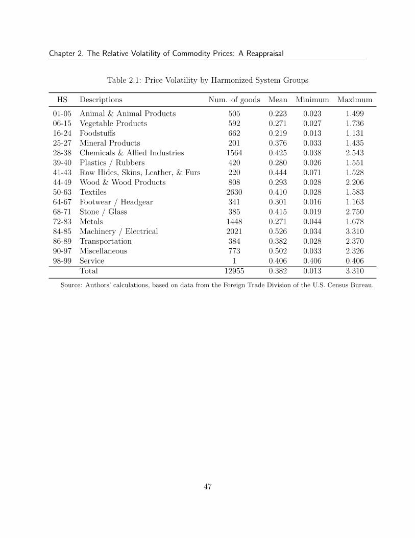
Chapter 2. The Relative Volatility of Commodity Prices: A Reappraisal
Table 2.1: Price Volatility by Harmonized System Groups
HS Descriptions Num. of goods Mean Minimum Maximum
01-05 Animal & Animal Products 505 0.223 0.023 1.49906-15 Vegetable Products 592 0.271 0.027 1.73616-24 Foodstuffs 662 0.219 0.013 1.13125-27 Mineral Products 201 0.376 0.033 1.43528-38 Chemicals & Allied Industries 1564 0.425 0.038 2.54339-40 Plastics / Rubbers 420 0.280 0.026 1.55141-43 Raw Hides, Skins, Leather, & Furs 220 0.444 0.071 1.52844-49 Wood & Wood Products 808 0.293 0.028 2.20650-63 Textiles 2630 0.410 0.028 1.58364-67 Footwear / Headgear 341 0.301 0.016 1.16368-71 Stone / Glass 385 0.415 0.019 2.75072-83 Metals 1448 0.271 0.044 1.67884-85 Machinery / Electrical 2021 0.526 0.034 3.31086-89 Transportation 384 0.382 0.028 2.37090-97 Miscellaneous 773 0.502 0.033 2.32698-99 Service 1 0.406 0.406 0.406
Total 12955 0.382 0.013 3.310
Source: Authors’ calculations, based on data from the Foreign Trade Division of the U.S. Census Bureau.
47
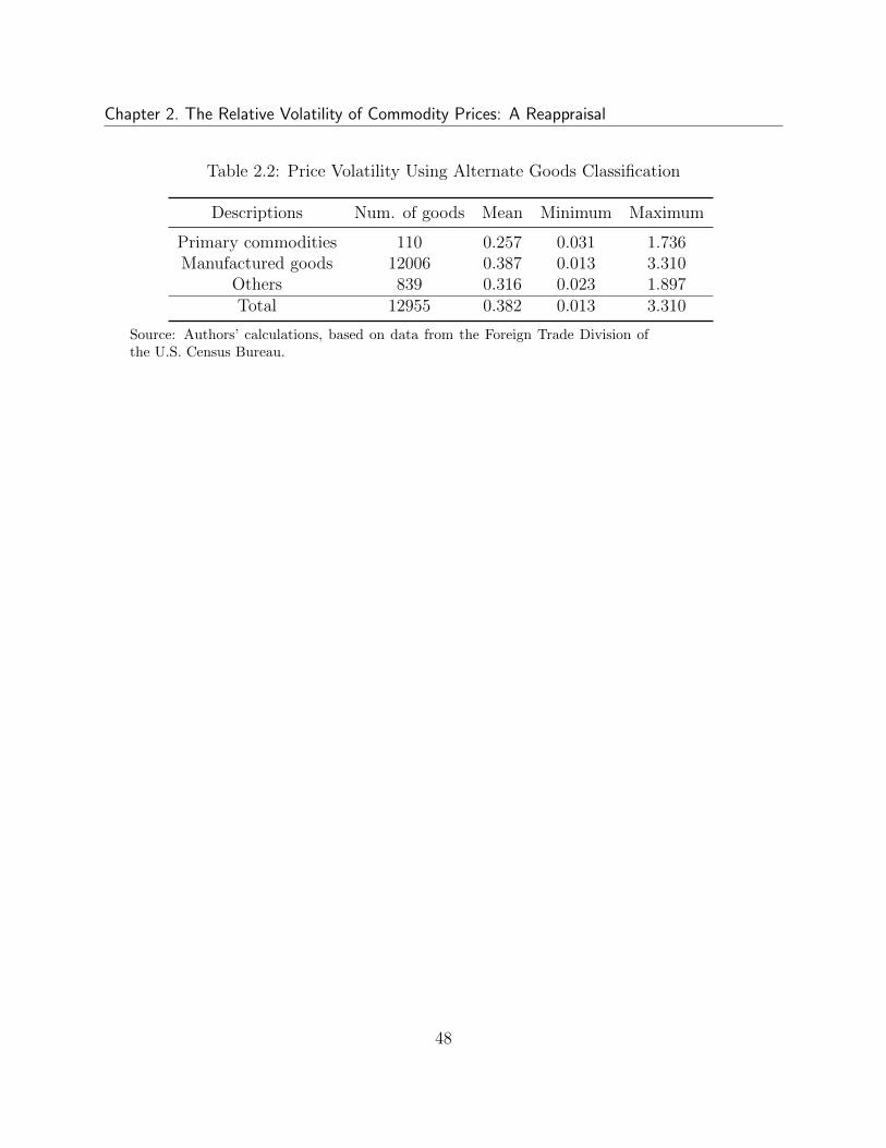
Chapter 2. The Relative Volatility of Commodity Prices: A Reappraisal
Table 2.2: Price Volatility Using Alternate Goods Classification
Descriptions Num. of goods Mean Minimum Maximum
Primary commodities 110 0.257 0.031 1.736Manufactured goods 12006 0.387 0.013 3.310
Others 839 0.316 0.023 1.897Total 12955 0.382 0.013 3.310
Source: Authors’ calculations, based on data from the Foreign Trade Division ofthe U.S. Census Bureau.
48
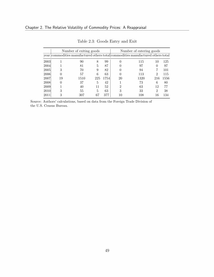
Chapter 2. The Relative Volatility of Commodity Prices: A Reappraisal
Table 2.3: Goods Entry and Exit
Number of exiting goods Number of entering goodsyear commodities manufactured others total commodities manufactured others total
2003 1 90 8 99 0 115 10 1252004 1 81 5 87 0 97 0 972005 3 70 9 82 0 94 7 1012006 0 57 6 63 0 113 2 1152007 19 1510 225 1754 20 1320 216 15562008 0 37 5 42 1 73 6 802009 1 40 11 52 2 63 12 772010 3 55 5 63 3 33 2 382011 3 307 67 377 10 108 16 134
Source: Authors’ calculations, based on data from the Foreign Trade Division ofthe U.S. Census Bureau.
49

Chapter 2. The Relative Volatility of Commodity Prices: A Reappraisal
Table 2.4: CDFs of Price Volatilities and the Level of Aggregation of Trade Data
Stochastic Dominance Test:Null Hypothesis
HS Level of Aggregation10 8 6 4 2
Commodity Price Volatility DominatesManufactured Price Volatility
K-S test statistic 0.034 0.255 0.227 0.697 0.563p-value 0.998 0.878 0.902 0.379 0.531
Manufactures Price Volatility DominatesCommodity Price Volatility
K-S test statistic 2.404 1.312 0.656 0.826 0.366p-value 0.000 0.032 0.423 0.256 0.765
CDFs of Price Volatilities are Equal Two-Sided Test p-value 0.000 0.042 0.699 0.376 0.670No. of manufactured 12006 5788 3598 983 77No. of commodities 110 33 26 10 5
Source: Authors’ calculations, based on data from the Foreign Trade Division of the U.S.Census Bureau – see text for details. Here the test means Kolmogorov-Smirnov test.
50
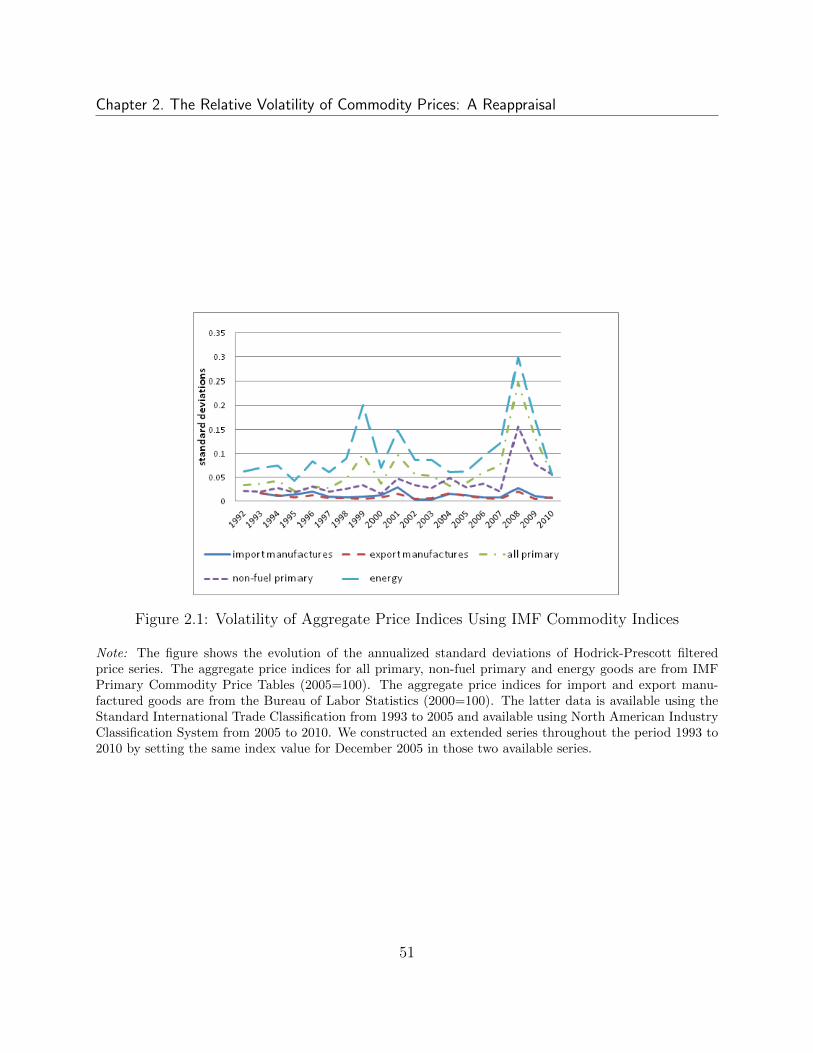
Chapter 2. The Relative Volatility of Commodity Prices: A Reappraisal
Figure 2.1: Volatility of Aggregate Price Indices Using IMF Commodity Indices
Note: The figure shows the evolution of the annualized standard deviations of Hodrick-Prescott filteredprice series. The aggregate price indices for all primary, non-fuel primary and energy goods are from IMFPrimary Commodity Price Tables (2005=100). The aggregate price indices for import and export manu-factured goods are from the Bureau of Labor Statistics (2000=100). The latter data is available using theStandard International Trade Classification from 1993 to 2005 and available using North American IndustryClassification System from 2005 to 2010. We constructed an extended series throughout the period 1993 to2010 by setting the same index value for December 2005 in those two available series.
51
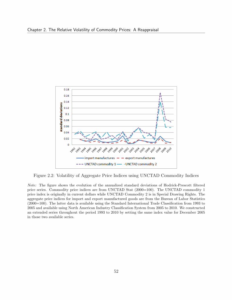
Chapter 2. The Relative Volatility of Commodity Prices: A Reappraisal
Figure 2.2: Volatility of Aggregate Price Indices using UNCTAD Commodity Indices
Note: The figure shows the evolution of the annualized standard deviations of Hodrick-Prescott filteredprice series. Commodity price indices are from UNCTAD Stat (2000=100). The UNCTAD commodity 1price index is originally in current dollars while UNCTAD Commodity 2 is in Special Drawing Rights. Theaggregate price indices for import and export manufactured goods are from the Bureau of Labor Statistics(2000=100). The latter data is available using the Standard International Trade Classification from 1993 to2005 and available using North American Industry Classification System from 2005 to 2010. We constructedan extended series throughout the period 1993 to 2010 by setting the same index value for December 2005in those two available series.
52
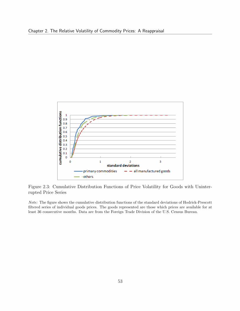
Chapter 2. The Relative Volatility of Commodity Prices: A Reappraisal
Figure 2.3: Cumulative Distribution Functions of Price Volatility for Goods with Uninter-rupted Price Series
Note: The figure shows the cumulative distribution functions of the standard deviations of Hodrick-Prescottfiltered series of individual goods prices. The goods represented are those which prices are available for atleast 36 consecutive months. Data are from the Foreign Trade Division of the U.S. Census Bureau.
53
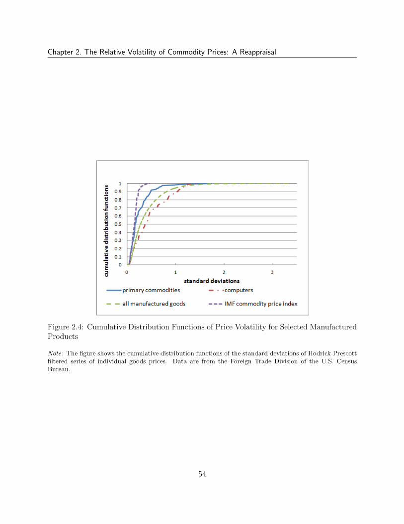
Chapter 2. The Relative Volatility of Commodity Prices: A Reappraisal
Figure 2.4: Cumulative Distribution Functions of Price Volatility for Selected ManufacturedProducts
Note: The figure shows the cumulative distribution functions of the standard deviations of Hodrick-Prescottfiltered series of individual goods prices. Data are from the Foreign Trade Division of the U.S. CensusBureau.
54

Chapter 2. The Relative Volatility of Commodity Prices: A Reappraisal
Figure 2.5: Cumulative Distribution Function of Price Volatility for Goods Available for theWhole Period
Note: The figure shows the cumulative distribution functions of the standard deviations of Hodrick-Prescottfiltered series of individual goods prices. The goods represented are those which prices are available for thewhole sample period. Data are from the Foreign Trade Division of the U.S. Census Bureau.
55

Chapter 2. The Relative Volatility of Commodity Prices: A Reappraisal
Figure 2.6: Cumulative Distribution Function of Volatility of Import Quantities
Note: The figure shows the cumulative distribution functions of the standard deviations of Hodrick-Prescottfiltered series of individual goods quantities. Data are from the Foreign Trade Division of the U.S. CensusBureau.
56
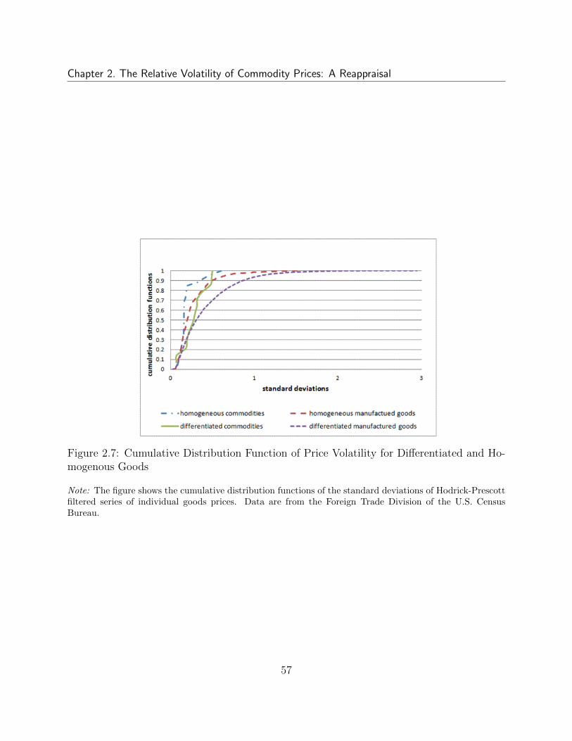
Chapter 2. The Relative Volatility of Commodity Prices: A Reappraisal
Figure 2.7: Cumulative Distribution Function of Price Volatility for Differentiated and Ho-mogenous Goods
Note: The figure shows the cumulative distribution functions of the standard deviations of Hodrick-Prescottfiltered series of individual goods prices. Data are from the Foreign Trade Division of the U.S. CensusBureau.
57
Chapter 3
The Relative Output Volatility andFinancial Development
3.1 Introduction
Understanding the economic volatilities is one of the central topics in the literature ofBusiness Cycles (Kydland and Prescott, 1982; Lucas, 1987). Macro economists have spentdecades in understanding the source of frictions in investment, labor and financial market,and searching for the channels that amplify exogenous shocks (Bernanke et al., 1999; Chariet al., 2007). One noticeable channel is the financial accelerator, which has been receivednew attention with global perspective, due to the recent global financial crisis and economicrecession. Mendoza (2010) shows that financial crash can lead to economic “sudden stop”through the mechanism of financial accelerator.
The essential spirit of Bernanke et al. (1999) is that the effect of Balance Sheet onfirms’ investment decision may amplify the impact of exogenous shocks such as interest rateschanges, leading to the fluctuations of aggregate economy. Previous cross-country analysesfocus on the relationship between the volatility of real output and financial friction, butignore the difference in the magnitude of exogenous shocks. The current paper presentsnew cross-country evidence of the relative output volatility and financial development, inparticular, we focus on the volatility ratio of nominal output to money stocks.1 Cross-country evidence shows that there is a negative correlation between the relative outputvolatility and financial development, and we show that it is consistent with an extended
1We use the volatility of money stock, rather than the volatility of nominal interest rate, as a measureof the magnitude of monetary shocks. It is because the nominal interest rate instruments are likely to bemanipulated by governments in many developing countries, which adopt inflation targeting monetary policyby controlling money supplies directly. Moreover, we find a weakly negative correlation between the realoutput volatility and financial development, but it makes more sense to use the relative volatility of outputbecause the magnitude of monetary shocks can be different across countries.
58
Chapter 3. The Relative Output Volatility and Financial Development
model of financial accelerator based on Bernanke et al. (1999).Our paper is firstly motivated by the observation of the volatilities of nominal GDP to
money stock (M2) in the US and China.2 Table 3.1 shows that the volatilities of moneystock (gM) and nominal output (gPY ) are both larger in China than in the US. 3 It is notsurprising to see that the Chinese economy is more volatile than the US, because it is afast-growing transitional economy. However, it is interesting to see that the volatility ratioof the output to money stock is much larger in China (more than 1) than in the U.S. (aboutone half).
Table 3.1 and Table 3.2 list the volatilities of money stock and nominal GDP’s growthrates for 22 (annual data) and 18 (quarterly data) countries individually. First, we observelarge variations in both the volatilities of money stocks and output, and there is a positivecorrelation between them. Basically, more volatile money stock is associated with moredramatic fluctuation of output. Second, we also observe a large variation of the relativevolatility of output to money stock. Notice that Mexico and India, just like China, have alarger ratio than 1, while the relative volatility ratio is smaller in UK and Denmark.
Figure 3.1 shows that the relative volatility of output to money stock is negatively cor-related with financial development level.4 It implies that the relative volatility of output issmaller in countries with better financial systems. Figure 3.2 shows a similar pattern for agroup of developed countries in which we use a different measure of financial index. 5 Ourconjecture is that countries with poorer financial system have larger output volatility due tothe stronger effect of financial accelerator mechanism, given the same monetary shocks.
We introduce the classic liquidity demand for money into the framework of Bernankeet al. (1999) model. This allows us to evaluate the relative volatility of output to moneydemand (in money market equilibrium it is equal to money stock). By doing so, we canevaluate the role of financial friction in the relative volatility of output. We calibrate themodel to both the U.S. and China, simulation exercise shows that the model can catch theempirical evidence that financial development and relative output volatility is negativelycorrelated.
This paper is organized as follows. Section 3.2 describes the literature of financial accel-erator. Section 3.3 describes the model. In section 3.4 we do simulation and show the resultscan replicate the empirical evidence. Section 3.5 presents concluding remarks.
2We use the standard deviation of de-trended time series data to assess the volatility. Here we reportresults based on the first difference filter, namely the growth rates, but all results reported herein also holdwith alternative filters, including the Hodrick-Prescott and Baxter-King band-pass filter.
3The sample period is between 1985 and 2008 because China has begun to build the modern bank systemand the central bank has started to release international comparable statistics since 1985.
4The sample size is small as we limit the countries which have consistent definition of money stock in IFSdataset.
5In Figure 3.1, the measure of financial development is FD score from world economic forum. In Figure3.2, it is financial index scores from IMF, 4th chapter of World Economic Outlook, September 2006.
59
Chapter 3. The Relative Output Volatility and Financial Development
3.2 Literature Review
Most economists agree that monetary policy can significantly influence the real economy, atleast in the short run (Friedman et al. (1989), Romer and Romer (1989),Christiano et al.(1996)). Conventional wisdom about how money influences real economy is that monetarypolicymakers use their leverage over short-term interest rate to influence the cost of capital,and consequently spending on fixed investment, housing, inventories and consumer durables.Changes in aggregate demand affect the level of production. But empirical studies show thatthe effect of cost-of-capital is weak. Also it is puzzling to see that monetary policy has largeeffects on purchase of long-term assets. Thus Bernanke and Gertler (1995) introduce financialfriction, so called credit channel, to explain those puzzles. They emphasize two channels.One is balance sheet channel, stressing the potential impact of changes in monetary policyon borrowers’ balance sheets and income statements, including variables such as borrowers’net worth, cash flow and liquid assets. Another is bank lending channel, focusing morenarrowly on the possible effect of monetary policy actions on the supply of loans by depositoryinstitutions.
The procyclical nature of net worth leads the external finance premium, the wedge be-tween the cost of external finance and internal funds, to fall during booms and to rise duringrecessions. Bernanke et al. (1999) and others, including Kiyotaki and Moore (1997) andCarlstrom and Fuerst (1997), demonstrate that these financial frictions may significantlyamplify the magnitude and the persistence of fluctuations in economic activity.
Bernanke et al. (1999) develop a model in which there is a two-way link between theborrowing costs of firms and their net worth. In their model, entrepreneurs, who borrowfunds to undertake investment projects, face an external finance premium that rises whentheir leverage increases. A tightening in monetary policy, for example, reduces the return oncapital and then the net worth of firms. The declines in net worth raise external financingcosts and reduce the demand for capital. The drop in demand for capital reinforces thedecline in its value. This mechanism is often called an accelerator effect, because the lowerprice of capital has a feedback effect, further lowering the net worth of firms.
Carlstrom and Fuerst (1997) find that the financial friction allows the model to bettermatch the key feature of the data: a hump-shaped output response to shocks in a standardreal business cycle model, but it did not amplify the response of output. Using a sticky-pricemodel calibrated to postwar US data, Bernanke et al. (1999) show that a different setupfor the financial-accelerator mechanism both amplifies the impact of shocks and provides aquantitatively important mechanism that propagates shocks at business cycle frequencies.
Meier and Muller (2005) estimate their model with US data by matching impulse re-sponses with the empirical ones to a monetary policy shock from a vector autoregression.Their findings attribute an important role to capital adjustment costs, but only a marginalrole to the accelerator in explaining the transmission of monetary policy shocks. They arguethat little is lost if DSGE models do not incorporate financial-accelerator effects. Chris-
60
Chapter 3. The Relative Output Volatility and Financial Development
tensen and Dib (2008) find that the accelerator mechanism plays an important role in thetransmission of monetary policy shocks.
3.3 Model
We follow the financial accelerator model discussed in Bernanke et al. (1999). The financialfriction is represented by “costly state verification”. The lender must pay a cost if he or shewishes to observe a borrower’s realized return on capital. The monitoring cost is assumedto be equal to a proportion (µ) of the realized gross payoff to the firm’s capital. Thus, µis a measure of financial development. It is smaller in a financially developed country andbigger in a less developed country. In order to control other differences between developedand developing countries, we will look at the effect of µ in a specified economy.
When µ increases, the lender must pay a larger proportion to know the real return ofcapital if the borrower defaults; thus the lender will ask for a bigger return premium. Theborrower then will decrease its borrowings and accumulate more net worth, therefore thesteady state capital-net worth ratio decreases. As money expands, values of net worthincrease and firms only need to pay a smaller risk premium to get loans. It stimulatesinvestment and therefore increases output. On the other side, if there is a negative shockto shrink money stock, the prices of goods and capital decrease which make the net worthof firms worthless. Risk premium will increase and prevent firms from buying a lot todo investment. Therefore the µ plays an important role in accelerating output to makeit more volatile than money stock. In the following model we will see in detail how thisparameter works. We add the money demand function into the basic model so that ingeneral equilibrium we can identify the role of µ on volatility of money and output.
3.3.1 Financial Friction
Let’s denote the profit per unit of capital as ωRk, where ω is an idiosyncratic shock to afirm’s return and Rk is the return to capital. Assume E(ω) = 1, F (x) = Pr(ω < x) is theCDF and f(ω) is the pdf of ω. The initial net worth of a firm is N, and the price of capital isQ. In order to invest a project which needs capital K, the firm has to borrow QK-N. Beforeinvestment ω is unknown to both firms and lender. After making the investment decision,the firm knows ω, but the lender has to pay some monitoring cost to know it. The cost isproportional (µ) to the total return of that firm.
If ω is quite large, the firm will have enough return to pay the loan back to the lender,and then get the left. The non-default loan rate is Z. But if ω is very small, the firm will goto bankruptcy and receive nothing. After paying the monitoring cost the lender will thenget the residual which is 1 − µ times the total capital payoff. Thus the cut-off ω is definedas ωRkQK = Z(QK −N). Let’s define the total capital payoff of default firms as:
61
Chapter 3. The Relative Output Volatility and Financial Development
G(ω) =∫ ω
0ωf(ω)dω
Then the total gross share of the capital payoff going to the lender isΓ(ω) = G(ω) + ω
∫∞ωf(ω)dω.
The net share to the lender is (1− µ)G(ω) + ω∫∞ωf(ω)dω.
For firms they want to get maximal payoff by choosing the quantity of capital K. Forlenders the expected return should be equal to the opportunity cost of their funds which isthe riskless rate R. Therefore the optimal contracting problem is:
maxK,ω
(1− Γ(ω))RkQK
s.t.[Γ(ω)− µG(ω)]RkQK = R(QK −N)
Let’s define the premium on external financing s = Rk/R, capital-wealth ratio k = QK/N ,and λ as the Lagrange multiplier on the constraint. After rearranging the first order condi-tions to K,ω, λ, we can get three equations for s, k, λ.
λ(ω) =1− F (ω)
1− F (ω)− µωf(ω)
s =λ(ω)
(1− Γ(ω)) + λ(Γ(ω)− µG(ω))
k = 1 +λ(Γ(ω)− µG(ω))
1− Γ(ω)
By calculation, we get ω′(s) > 0, k′(ω) > 0 and thus ∂s∂k> 0. It is the most important
result in our analysis. If a firm has relatively large ratio of net worth to the total capitalrequired, then the risk premium the lender would like to charge is relatively small; thus inequilibrium the firm gets more capital and invest more.
Then, the supply of extern financing is defined by the below equation.
E(Rkt ) = s(
Nt
Qt−1Kt
)Rt (3.1)
3.3.2 Household
In the model, there is a continuum of households. Each household works, consumes, holdsmoney, and deposits. Let’s denote Ct as consumption, Ht as labor supply, Dt as deposit,Mt as money holdings, Wt as real wage, Rt as riskless interest rate, Πt as dividends from
62
Chapter 3. The Relative Output Volatility and Financial Development
ownership of retail firms, Tt as tax. Then the household problem is:
maxCt,Ht,Dt,Mt
EtΣ∞k=0β
k[ln(Ct+k) + ςln(Mt+k/Pt+k)−H
1+ 1η
t+k
1 + 1η
]
s.t.Ct = wtHt −TtPt
+Πt
Pt+RtDt −Dt+1 +
Mt−1 −Mt
Pt
Arranging the first order conditions, we can get the following equations.
1
Ct=
β
Ct+1
Rt (3.2)
H1η
t =Wt
Ct(3.3)
Mt
Pt= ςCt
Rt · Pt+1
Pt− 1
Rt · Pt+1
Pt
(3.4)
3.3.3 Enterprise Sector
First, we assume the labor input is composed of two parts: household labor Ht and en-trepreneurial labor He
t . Lt = HΩt (He
t )1−Ω. For the enterprises which produce the wholesale
goods, they hire house labor at wage rate Wt, give entrepreneurial labor wage rate W et and
rent capital at rate Rkt to produce and sell at a relative price of 1/Xt. Their optimal problem
is:
maxHt,He
t ,Kt
∏t
=1
Xt
Yt −WtHt −W et H
et −Rk
tQt−1Kt−1 + (1− δ)QtKt−1
s.t.Yt = AtKαt−1H
(1−α)Ωt (He
t )(1−α)(1−Ω)
The first order conditions are:
Wt = Ω(1− α)Yt
XtHt
(3.5)
W et = (1− Ω)(1− α)
YtXtHe
t
(3.6)
Rkt =
α YtXtKt−1
+ (1− δ)Qt
Qt−1
(3.7)
Yt = AtKαt−1H
(1−α)Ωt (He
t )(1−α)(1−Ω) (3.8)
63
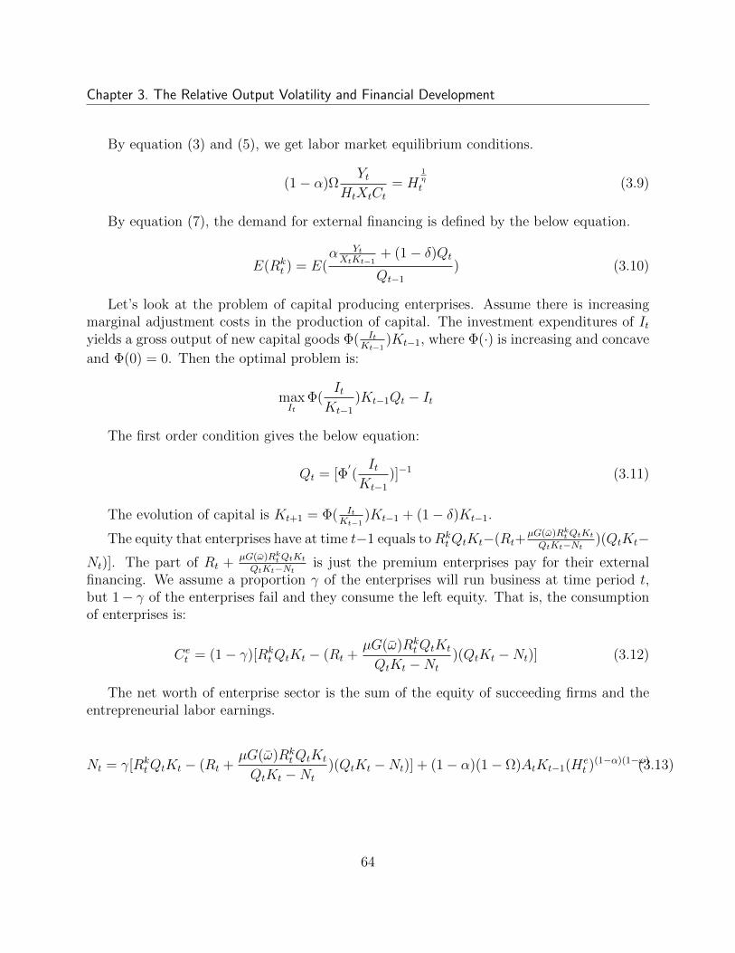
Chapter 3. The Relative Output Volatility and Financial Development
By equation (3) and (5), we get labor market equilibrium conditions.
(1− α)ΩYt
HtXtCt= H
1η
t (3.9)
By equation (7), the demand for external financing is defined by the below equation.
E(Rkt ) = E(
α YtXtKt−1
+ (1− δ)Qt
Qt−1
) (3.10)
Let’s look at the problem of capital producing enterprises. Assume there is increasingmarginal adjustment costs in the production of capital. The investment expenditures of Ityields a gross output of new capital goods Φ( It
Kt−1)Kt−1, where Φ(·) is increasing and concave
and Φ(0) = 0. Then the optimal problem is:
maxIt
Φ(It
Kt−1
)Kt−1Qt − It
The first order condition gives the below equation:
Qt = [Φ′(It
Kt−1
)]−1 (3.11)
The evolution of capital is Kt+1 = Φ( ItKt−1
)Kt−1 + (1− δ)Kt−1.
The equity that enterprises have at time t−1 equals toRktQtKt−(Rt+
µG(ω)RktQtKtQtKt−Nt )(QtKt−
Nt)]. The part of Rt +µG(ω)RktQtKtQtKt−Nt is just the premium enterprises pay for their external
financing. We assume a proportion γ of the enterprises will run business at time period t,but 1− γ of the enterprises fail and they consume the left equity. That is, the consumptionof enterprises is:
Cet = (1− γ)[Rk
tQtKt − (Rt +µG(ω)Rk
tQtKt
QtKt −Nt
)(QtKt −Nt)] (3.12)
The net worth of enterprise sector is the sum of the equity of succeeding firms and theentrepreneurial labor earnings.
Nt = γ[RktQtKt − (Rt +
µG(ω)RktQtKt
QtKt −Nt
)(QtKt −Nt)] + (1− α)(1− Ω)AtKt−1(Het )
(1−α)(1−ω)(3.13)
64

Chapter 3. The Relative Output Volatility and Financial Development
3.3.4 Log-linearized Equations
To complete the model, we add the equilibrium conditions. In equilibrium, the goods marketis clear.
Yt = Ct + It +Gt + Cet (3.14)
The shocks that we consider here are exogenous disturbances to nominal interest rate,technology and government expenditure. They are autoregressive processes.
Gt = Gρgt−1 ∗ ε
gt (3.15)
At = Aρat−1 ∗ εat (3.16)
Rnt = R
nρgt−1 ∗ εrnt (3.17)
Also we introduce traditional money demand equation into the model. Real moneydemand is a function of real output and nominal interest rate. It increases with the increaseof real output and (or) the decrease of nominal interest rate.
We use lower case to denote deviations from steady state. Then the whole log-linearized
65

Chapter 3. The Relative Output Volatility and Financial Development
model is composed of the following equations.
yt =C
Yct +
I
Yit +
G
Ygt +
Ce
Ycet
ct = −rt + ct+1
cet = nt
rkt+1 − rt = −v[nt − (qt + kt)]
rkt = (1− ε)(yt − kt−1 − xt) + εqt − qt−1
qt = ψ(it − kt−1)
yt = at + αkt−1 + (1− α)Ωht
yt − ht − xt − ct =1
ηht
πt = κxt + βπt+1
kt+1 = δit + (1− δ)kt−1
nt =γRK
N(rkt − rt−1) + rt−1 + nt−1
rnt = ρrnt−1 + ζπt−1 + εrntgt = ρggt−1 + εgtat = ρaat−1 + εatrnt = rt + πt+1
mt + xt = φyyt − φrrnt
3.4 Simulations
3.4.1 Parameters and Coefficients
To choose the values of parameters in the log-linearized equations, we followed the paper ofFisher (1999), Carlstrom and Fuerst (1997), Clarida et al. (2000), and Bernanke et al. (1999)(See Table 3.3).
In order to solve the model, we need to fix some steady state values. There are somecoefficients which are strictly affected by the value and the distribution of µ, like Rk, K/N ,X, and Y/K. If we change the value of µ, the return premium varies and thus the requiredreturn to the capital does. The steady state ratio of capital to net worth will change too.The leverage ratio decreases with higher financial friction.
In steady states, βR = 1, thus we know the value of R = 1/β. For the share of governmentexpenditure to the total output, we use the historical average (0.2) like Bernanke et al. (1999).
66
Chapter 3. The Relative Output Volatility and Financial Development
The share of income to entrepreneurs’ labor is 0.01 given Ω = 0.99. We use the historicalaverage data to estimate C/Y and then compute I/Y = 1− C/Y −G/Y − Ce/Y . For theincome and interest rate elasticity of money demand, we use the long-run estimators: 1 and-0.6. Different values of φy and φi change the absolute values of the variance ratio, but thenegative correlations between µ and variance ratio still exist. This is what we want to get.Using the parameters in Table 3.3 and the steady states values, we can directly calculate εand κ.
3.4.2 Simulation Results
Consider a positive monetary shock, nominal interest rate unanticipated decreases 0.25points. Here the time period we use is in quarters. Following the regular assumption,µ = 0.12, the impulse response functions are shown in Figure 3.3. The impulse response ofoutput does not have humped shape like the VAR evidence, but this question will be solvedby adding investment delay (See appendix A.2).6
Then let’s look at the case of µ = 0.52, which is a random value bigger than 0.12 that wechoose. Comparing with the benchmark case, the larger the µ is, the larger the responses ofmajor variables are (Figure 3.4).
Next we show the correlation between µ and the volatility ratio (std(PY )/std(M)).Choosing T=100, we see a downward sloping curve (Figure 3.5).7 With the decrease of µ,which means the financial conditions get better, the relative volatility of output to money issmaller. This is exactly what we have seen in the empirical facts.
Also, Figure 3.6 shows the calibration of China’s case, and it has a similar pattern likethe benchmark case of US.8
3.4.3 Parameters Sensitivity Check
In the appendix A.4, we plot the figures of parameters robust check. ρa and ρg have noimpact since we only consider the monetary shock. α should be bigger than 0.3, η is lessthan 0.5, δ is less than 0.1, θ is bigger than 0.2, γ is bigger than 0.4, F (ω) is less than 0.5,Variance of ω is bigger than 0.6, and ρ needs bigger than 0.89. As long as all the parameterstake the above reasonable values, we can get the negative correlation between µ and volatilityratio std(gPY )/std(gM). The simulated results are not affected by the choice of parameters’values.
6The results reported herein hold if we add investment delay.7Here one period is one quarter, thus 100 means 25 years. It is long enough to show the effect of shocks.8To calibrate China, I modified the following parameters: depreciation rate for capital (δ = 0.025),
response of nominal interest rate to lagged inflation (ζ = 0.04), serial correlation of nominal interest rate(ρ = 0.96), death rate (1 − γ = 0.3), entrepreneurial consumption share (Ce/Y = 0.02), steady-state shareof government expenditures (G/Y = 0.1437), consumption share to GDP (C/Y = 0.4517)
67
Chapter 3. The Relative Output Volatility and Financial Development
3.4.4 Quantitative Analysis
Until now our simulation results are qualitatively similar as the empirical evidence. In orderto see the model performance, let’s do quantitative analysis. Since it is hard to define µ inreality, we need to turn to an intermediate statistics. In the model, the interest premiumfluctuates more as µ increases. It not only leads to bigger variance ratio, but also a smallerratio of credit to output. Credit is the total capital purchased and invested by entrepreneurminus the net worth it has. It is just what the entrepreneurs borrow. See Figure 3.7 for thecorrelation of µ and credit/(PY).
By Figure 3.5 and 3.7, we can infer there is a negative correlation between the ratio ofcredit to output and the variance ratio. Figure 3.8 is the simulated result of credit/(PY)and variance ratio std(gPY )/std(gM).
We would like to find a measure of credit, and then divide it by nominal GDP to get theratio of credit/(PY) in real world. By adjusting parameters we can let the simulated ratiothe same number as the real one.
In Flow of Funds Accounts of the United States, there is a measure of credit marketdebt outstanding.9 It is a stock but not flow variable, just like the credit definition in ourmodel. We add credit market debt outstanding of household sector, non-financial corporatebusiness, nonfarm noncorporate business, and farm business together to get the domesticdebts without government. It is consistent with our definition in the model. Dividing thisvariable by nominal GDP we get credit/(PY). Taking average for 1985-2005, the value is1.36.
Slightly adjusting some parameters values, η decreases from 3 to 1 and var(ω) increasesfrom 0.282 to 0.62. We can get simulated value of credit/PY, which is 1.36. We change ψfrom 0.25 to 2 and then the simulated value of std(PY )/std(M) approaches the real one0.53.10 Ideally if we have other countries credit data, we can compare it with the value gotfrom calibration by US parameters. Then we can tell to what extent the output volatilitydifference among countries is caused by the difference of financial development. This is myfuture work.
3.5 Conclusions
In this paper, we reveal the correlation between relative output volatility and financial de-velopment using cross country data. Then we expand the financial accelerator model toexplain such a correlation. With poorer financial conditions, the changes of asset prices leadto dramatic fluctuations of net worth, and thus the wedge between external and internal
9It is table L.1, end of period measurement. Unit is billions of dollars and the frequency is annually.10King and Wolman (1996) also uses a value of 2 based on estimates from aggregate data by Chirinko
(1993).
68

Chapter 3. The Relative Output Volatility and Financial Development
financing cost is bigger. The stronger effect of financial accelerator mechanism accounts forthe larger volatility of output to money. The simulation results are also consistent with theempirical facts.
69
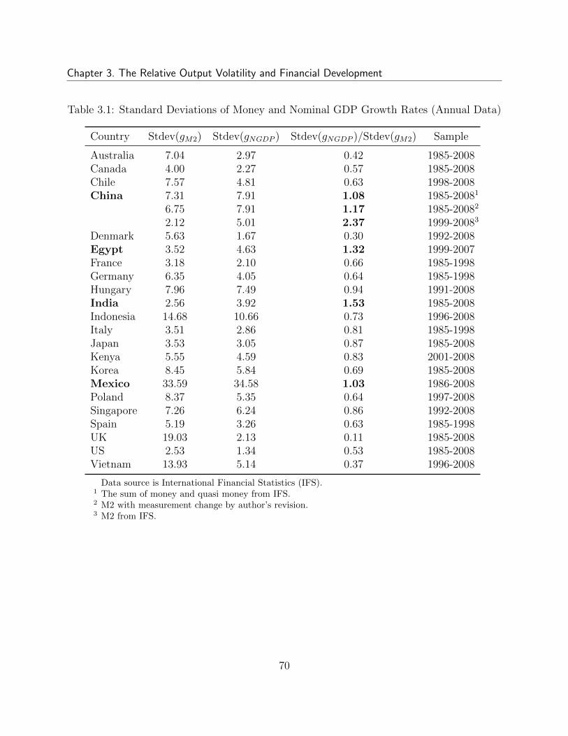
Chapter 3. The Relative Output Volatility and Financial Development
Table 3.1: Standard Deviations of Money and Nominal GDP Growth Rates (Annual Data)
Country Stdev(gM2) Stdev(gNGDP ) Stdev(gNGDP )/Stdev(gM2) Sample
Australia 7.04 2.97 0.42 1985-2008Canada 4.00 2.27 0.57 1985-2008Chile 7.57 4.81 0.63 1998-2008China 7.31 7.91 1.08 1985-20081
6.75 7.91 1.17 1985-20082
2.12 5.01 2.37 1999-20083
Denmark 5.63 1.67 0.30 1992-2008Egypt 3.52 4.63 1.32 1999-2007France 3.18 2.10 0.66 1985-1998Germany 6.35 4.05 0.64 1985-1998Hungary 7.96 7.49 0.94 1991-2008India 2.56 3.92 1.53 1985-2008Indonesia 14.68 10.66 0.73 1996-2008Italy 3.51 2.86 0.81 1985-1998Japan 3.53 3.05 0.87 1985-2008Kenya 5.55 4.59 0.83 2001-2008Korea 8.45 5.84 0.69 1985-2008Mexico 33.59 34.58 1.03 1986-2008Poland 8.37 5.35 0.64 1997-2008Singapore 7.26 6.24 0.86 1992-2008Spain 5.19 3.26 0.63 1985-1998UK 19.03 2.13 0.11 1985-2008US 2.53 1.34 0.53 1985-2008Vietnam 13.93 5.14 0.37 1996-2008
Data source is International Financial Statistics (IFS).1 The sum of money and quasi money from IFS.2 M2 with measurement change by author’s revision.3 M2 from IFS.
70

Chapter 3. The Relative Output Volatility and Financial Development
Table 3.2: Standard Deviations of Money and Nominal GDP Growth Rates (Quarterly Data)
Country Stdev(gM2) Stdev(gNGDP ) Stdev(gNGDP )/Stdev(gM2) Sample
Australia 7.18 3.27 0.46 1985q1-2009q3Canada 4.00 3.23 0.81 1985q1-2009q3Chile 7.30 5.98 0.82 1998q4-2009q3China 3.66 9.06 2.47 2000q1-2009q3
6.22 8.97 1.44 1993q1-2009q31
Denmark 5.25 2.75 0.52 1992q1-2009q3France 3.36 2.25 0.67 1984q1-1998q4Germany 6.71 5.46 0.81 1984q1-1998q4Hungary 4.28 7.33 1.71 1996q1-2009q3India 3.63 6.40 1.76 2005q1-2009q3Indonesia 15.26 10.99 0.72 1996q1-2009q3Italy 4.14 3.20 0.77 1984q1-1998q4Korea 8.28 5.95 0.72 1984q1-2008q4Mexico 33.52 34.99 1.04 1986q4-2009q3Poland 7.89 4.39 0.56 1997q4-2009q3Singapore 5.47 6.96 1.27 2004q1-2009q2Spain 5.15 3.25 0.63 1984q1-1998q4UK 18.45 2.81 0.15 1984q1-2009q3US 2.41 1.94 0.81 1984q1-2009q3
Data source is International Financial Statistics (IFS).1 we construct the quarterly GDP data from 1993Q1 to 1999Q4 by using yearly data.
71
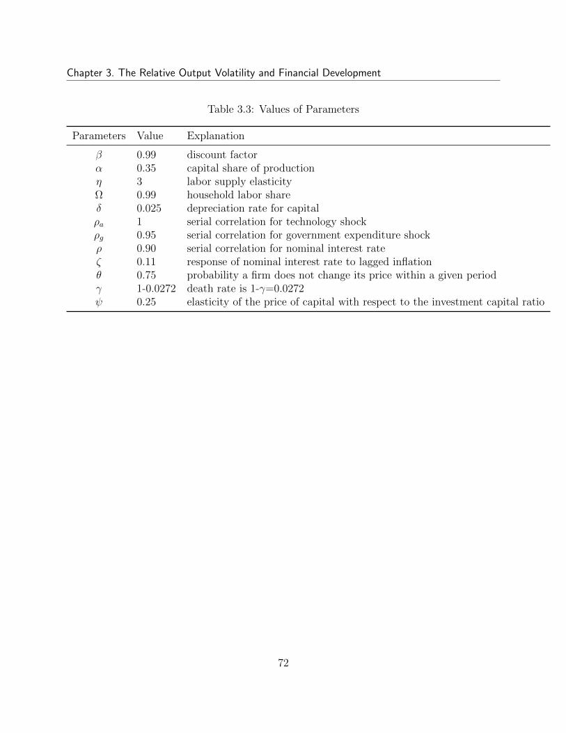
Chapter 3. The Relative Output Volatility and Financial Development
Table 3.3: Values of Parameters
Parameters Value Explanation
β 0.99 discount factorα 0.35 capital share of productionη 3 labor supply elasticityΩ 0.99 household labor shareδ 0.025 depreciation rate for capitalρa 1 serial correlation for technology shockρg 0.95 serial correlation for government expenditure shockρ 0.90 serial correlation for nominal interest rateζ 0.11 response of nominal interest rate to lagged inflationθ 0.75 probability a firm does not change its price within a given periodγ 1-0.0272 death rate is 1-γ=0.0272ψ 0.25 elasticity of the price of capital with respect to the investment capital ratio
72

Chapter 3. The Relative Output Volatility and Financial Development
Figure 3.1: Financial Development and Volatility Ratio
73
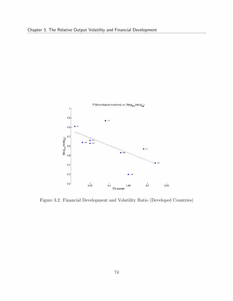
Chapter 3. The Relative Output Volatility and Financial Development
Figure 3.2: Financial Development and Volatility Ratio (Developed Countries)
74
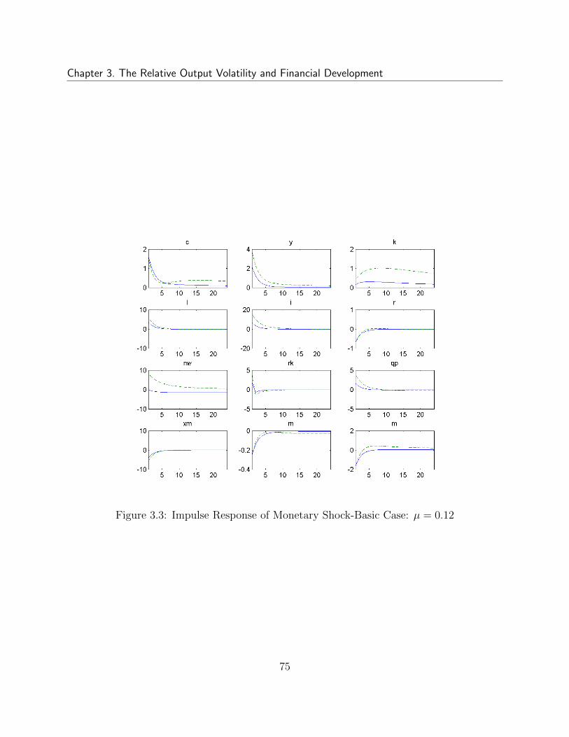
Chapter 3. The Relative Output Volatility and Financial Development
Figure 3.3: Impulse Response of Monetary Shock-Basic Case: µ = 0.12
75
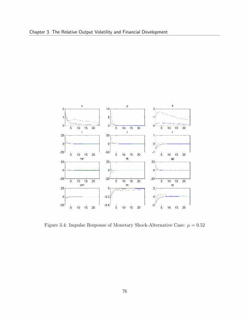
Chapter 3. The Relative Output Volatility and Financial Development
Figure 3.4: Impulse Response of Monetary Shock-Alternative Case: µ = 0.52
76
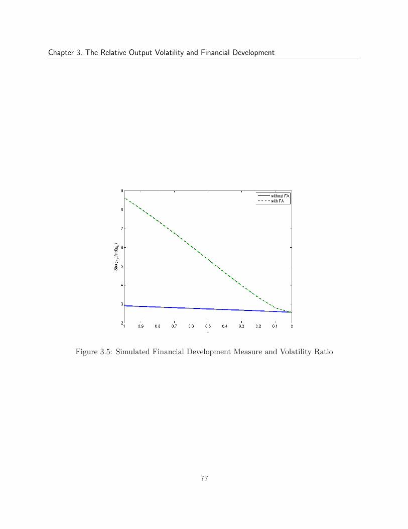
Chapter 3. The Relative Output Volatility and Financial Development
Figure 3.5: Simulated Financial Development Measure and Volatility Ratio
77
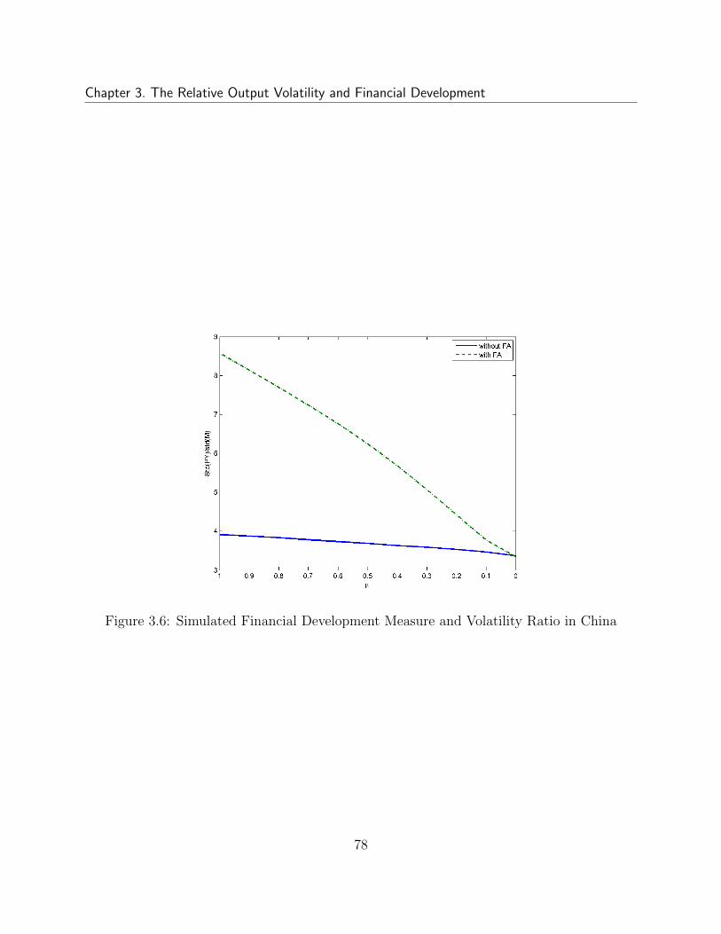
Chapter 3. The Relative Output Volatility and Financial Development
Figure 3.6: Simulated Financial Development Measure and Volatility Ratio in China
78
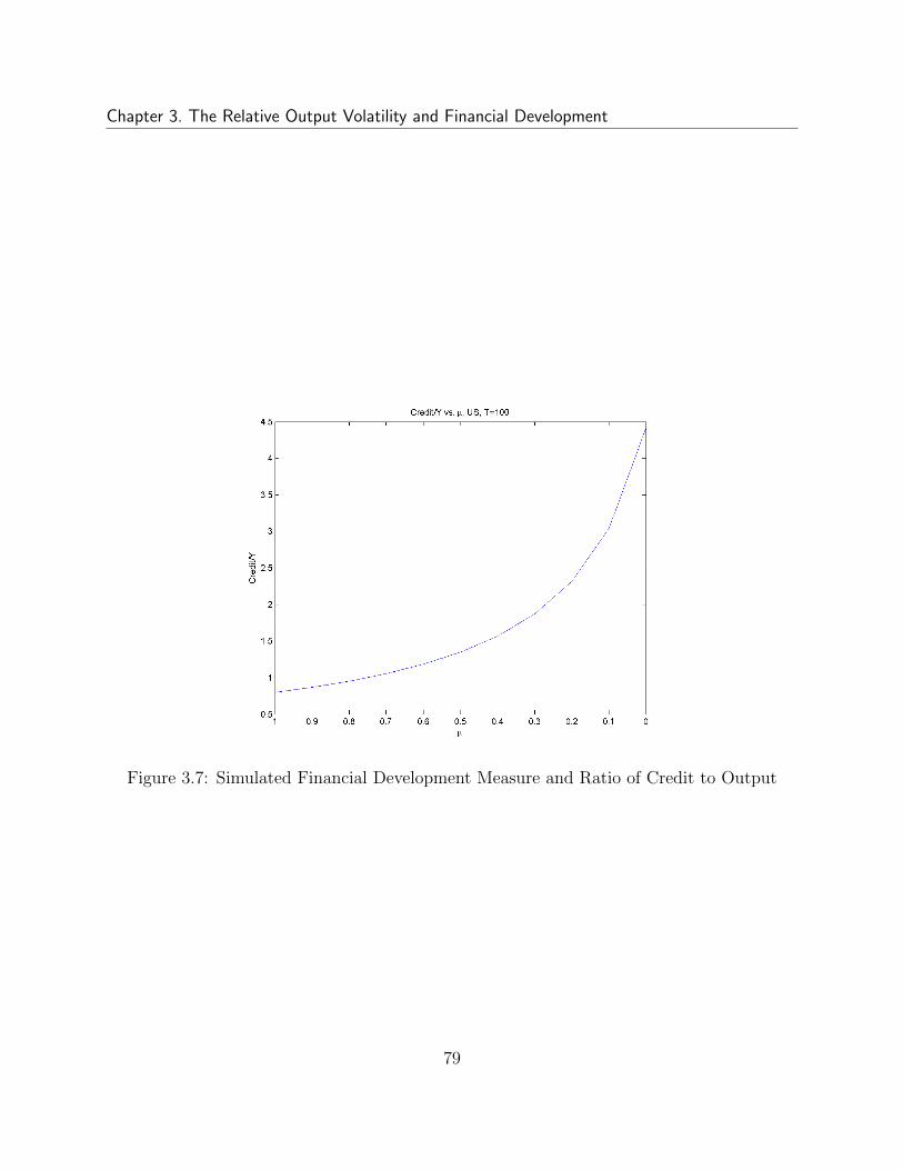
Chapter 3. The Relative Output Volatility and Financial Development
Figure 3.7: Simulated Financial Development Measure and Ratio of Credit to Output
79
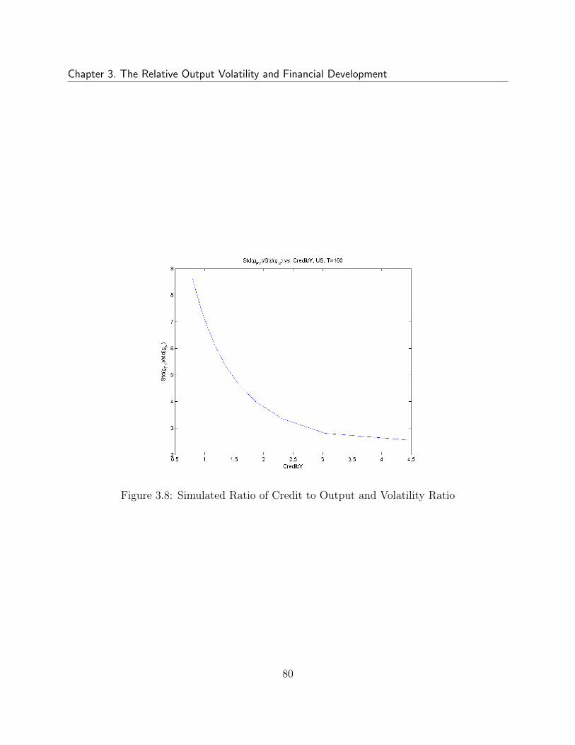
Chapter 3. The Relative Output Volatility and Financial Development
Figure 3.8: Simulated Ratio of Credit to Output and Volatility Ratio
80
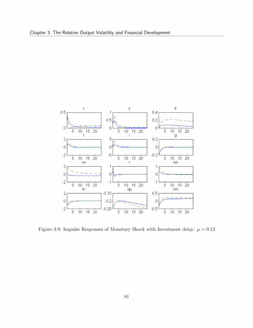
Chapter 3. The Relative Output Volatility and Financial Development
Figure 3.9: Impulse Responses of Monetary Shock with Investment delay: µ = 0.12
81
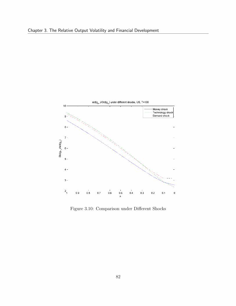
Chapter 3. The Relative Output Volatility and Financial Development
Figure 3.10: Comparison under Different Shocks
82
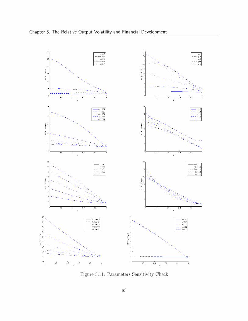
Chapter 3. The Relative Output Volatility and Financial Development
Figure 3.11: Parameters Sensitivity Check
83
Appendix A
A.1 Lists of Commodities under the IMF Primary Com-
modity Price Tables and UNCTAD Classifications
IMF Primary Commodity Price Tables: Aluminum, bananas, barley, beef, butter, coal, co-coa beans, coconut oil, coffee, copper, copra, cotton, DAP, fish, fish meal, gasoline, gold,groundnuts, groundnut oil, hides, iron ore, jute, lamb, lead, linseed oil, maize, natural gas,newsprint, nickel, olive oil, oranges, palm kernel oil, palm oil, pepper, petroleum, phosphaterock, potash, poultry, plywood, pulp, rice, rubber, shrimp, silver, sisal, sorghum, soybeans,soybean meal, soybean oil, sugar, sunflower oil, superphosphate, swine meat, tea, timber,hardwood logs, hardwood sawnwood, softwood logs, softwood sawnwood, tin, tobacco, ura-nium, urea, wheat, wool, zinc.
UNCTAD: Aluminum, bananas, beef, cattle hides, coarse wool, cocoa beans, coconutoil, coffee, copper, copra, cotton, cottonseed oil, crude petroleum, fine wool, fish meal, gold,groundnut oil, iron ore, jute, lead, linseed oil, maize, manganese ore, nickel, non-coniferouswoods, palm kernel oil, palm oil, pepper, phosphate rock, plywood, rice, rubber, silver, sisal,soybean oil, soybeans, soybean meal, sugar, sunflower oil, tea, tin, tobacco, tropical logs,tropical sawnwood, tungsten ore, wheat, zinc.
A.2 The Case with Investment Delay
Different from the basic model in the text, we consider the case with investment delay. SeeFigure 3.9 of the impulse response functions for the same µ like Figure 3.3, output hashumped shape like the VAR evidence.
84

Chapter A. Appendices
A.3 Other Shocks
In the basic model, if the shocks are not from the changes of interest rate, but from thechanges of technology or government expenditure, then we still get downward sloping curves(Figure 3.10).
A.4 Parameters Sensitivity Check
We do robust checks for main parameters: α, η, δ, θ, γ, F (ω), V ar(ω) and ρ. See Figure3.11 for the simulation results.
85
Bibliography
Aizenman, J., Lee, J., 2007. International reserves: precautionary versus mercantilist views, theoryand evidence. Open Economies Review 18 (2), 191–214.
Aizenman, J., Lee, J., 2008. Financial versus monetary mercantilism: Long-run view of largeinternational reserves hoarding. The World Economy 31 (5), 593–611.
Arezki, R., Bruckner, M., 2011. Food prices and political instability. No. 3544. International Mon-etary Fund.
Backus, D., Kehoe, P., 1992. International evidence on the historical properties of business cycles.The American Economic Review, 864–888.
Bai, C.-E., Hsieh, C.-T., Qian, Y., 2006. The return to capital in china. Brookings Papers onEconomic Activity 37 (2), 61–102.
Barrett, G., Donald, S., 2003. Consistent tests for stochastic dominance. Econometrica 71 (1),71–104.
Bernanke, B., Gertler, M., 1995. Inside the black box: the credit channel of monetary policytransmission. The Journal of Economic Perspectives 9 (4), 27–48.
Bernanke, B. S., Gertler, M., Gilchrist, S., 1999. Chapter 21 the financial accelerator in a quanti-tative business cycle framework. Vol. 1, Part C of Handbook of Macroeconomics. Elsevier, pp.1341 – 1393.
Brandt, L., Zhu, X., 2010. Accounting for china’s growth.
Bruckner, M., Ciccone, A., 2010. International commodity prices, growth and the outbreak of civilwar in sub-saharan africa*. The Economic Journal 120 (544), 519–534.
Caballero, R., Farhi, E., Gourinchas, P., 2008a. An equilibrium model of global imbalances and lowinterest rates. American Economic Review 98 (1), 358–393.
Caballero, R., Farhi, E., Gourinchas, P., 2008b. Financial crash, commodity prices and globalimbalances. Tech. rep., National Bureau of Economic Research.
86
BIBLIOGRAPHY
Calvo, G., Izquierdo, A., Talvi, E., 2006. Phoenix miracles in emerging markets: recovering withoutcredit from systemic financial crises. Tech. rep., National Bureau of Economic Research.
Calvo-Gonzalez, O., Shankar, R., Trezzi, R., 2010. Are commodity prices more volatile now? along-run perspective. A Long-Run Perspective (October 1, 2010). World Bank Policy ResearchWorking Paper Series, Vol.
Carlstrom, C., Fuerst, T., 1997. Agency costs, net worth, and business fluctuations: A computablegeneral equilibrium analysis. The American Economic Review, 893–910.
Cashin, P., McDermott, C., 2002. The long-run behavior of commodity prices: small trends andbig variability. IMF staff Papers, 175–199.
Chamon, M., Prasad, E., 2010. Why are saving rates of urban households in china rising? AmericanEconomic Journal: Macroeconomics 2 (1), 93–130.
Chari, V. V., Kehoe, P. J., McGrattan, E. R., 2007. Business cycle accounting. Econometrica 75 (3),781–836.
Cheung, Y., Chinn, M., Fujii, E., 2007. The overvaluation of renminbi undervaluation. Journal ofInternational Money and Finance 26 (5), 762–785.
Cheung, Y.-W., Chinn, M. D., Fujii, E., 2010. China’s current account and exchange rate. In:Feenstra, R. C., Wei, S.-J. (Eds.), China’s Growing Role in World Trade. University of ChicagoPress, pp. 231–271.
Chirinko, R., 1993. Business fixed investment spending: Modeling strategies, empirical results, andpolicy implications. Journal of Economic Literature 31 (4), 1875–1911.
Christensen, I., Dib, A., 2008. The financial accelerator in an estimated new keynesian model.Review of Economic Dynamics 11 (1), 155 – 178.
Christiano, L., Eichenbaum, M., Evans, C., 1996. The effects of monetary policy shocks: evidencefrom the flow of funds. The Review of Economics and Statistics 78 (1), 16–34.
Clarida, R., Gali, J., Gertler, M., 2000. Monetary Policy Rules and Macroeconomic Stability:Evidence and Some Theory. Quarterly Journal of Economics 115 (1), 147–180.
Deaton, A., Laroque, G., 1992. On the behaviour of commodity prices. The Review of EconomicStudies 59 (1), 1–23.
Deaton, A., Laroque, G., 2003. A model of commodity prices after sir arthur lewis. Journal ofDevelopment Economics 71 (2), 289–310.
Delgado, M., Farinas, J., Ruano, S., 2002. Firm productivity and export markets: a non-parametricapproach. Journal of international Economics 57 (2), 397–422.
87
BIBLIOGRAPHY
Dooley, M., Folkerts-Landau, D., Garber, P., 2003. An essay on the revived Bretton Woods system.NBER Working Paper.
Dooley, M., Folkerts-Landau, D., Garber, P., 2004a. The revived Bretton Woods system: Theeffects of periphery intervention and reserve management on interest rates & exchange rates incenter countries. NBER Working Paper.
Dooley, M., Folkerts-Landau, D., Garber, P., 2004b. Direct investment, rising real wages and theabsorption of excess labor in the periphery. NBER Working Paper.
Du, Q., Wei, S., 2010. A sexually unbalanced model of current account imbalances.
Durdu, C., Mendoza, E., Terrones, M., 2009. Precautionary demand for foreign assets in suddenstop economies: An assessment of the new mercantilism. Journal of Development Economics89 (2), 194–209.
Epstein, L., 1983. Stationary cardinal utility and optimal growth under uncertainty. Journal ofEconomic Theory 31 (1), 133–152.
Feenstra, R., Romalis, J., Schott, P., 2002. Us imports, exports, and tariff data, 1989-2001. Tech.rep., National Bureau of Economic Research.
Fisher, J., 1999. Credit Market Imperfections and the Heterogeneous Response of Firms to Mone-tary Shocks. Journal of Money, Credit & Banking 31 (2), 187–188.
Frankel, J., 2010. Natural resource curse: A survey of the literature. forthcoming in Commod-ity Prices and Inclusive Growth in Low-Income Countries, eds, Arezki, Pattillo and Quintyn,International Monetary Fund.
Friedman, M., Schwartz, A., of Economic Rese, Y. N. B., 1989. A monetary history of the UnitedStates. Princeton University Press.
Harvey, D., Kellard, N., Madsen, J., Wohar, M., 2010. The prebisch-singer hypothesis: four cen-turies of evidence. The review of Economics and Statistics 92 (2), 367–377.
He, D., Cheung, L., Zhang, W., Wu, T., 2012. How would capital account liberalisation affectchinas capital flows and the renminbi real exchange rates?
Hsieh, C.-T., Klenow, P. J., 2009. Misallocation and manufacturing tfp in china and india*. Quar-terly Journal of Economics 124 (4), 1403–1448.
Hummels, D., Klenow, P. J., 2005. The variety and quality of a nation’s exports. American EconomicReview 95 (3), 704–723.
Jacks, D., O’Rourke, K., Williamson, J., 2011. Commodity price volatility and world market inte-gration since 1700. Review of Economics and Statistics 93 (3), 800–813.
88
BIBLIOGRAPHY
Jeanne, O., Ranciere, R., 2011. The optimal level of international reserves for emerging marketcountries: A new formula and some applications*. The Economic Journal 121 (555), 905–930.
King, R., Wolman, A., 1996. Inflation targeting in a St. Louis model of the 21st century.
Kiyotaki, N., Moore, J., 1997. Credit cycles. Journal of political economy 105 (2), 211–248.
Kydland, F., Prescott, E., 1982. Time to build and aggregate fluctuations. Econometrica: Journalof the Econometric Society, 1345–1370.
Lederman, D., Maloney, W., 2007. Natural resources, neither curse nor destiny. Stanford Economicsand Finance.
Lucas, R., 1987. Models of business cycles.
Meier, A., Muller, G., 2005. Fleshing out the monetary transmission mechanism: Output compo-sition and the role of financial frictions. ECB Working Paper.
Mendoza, E., 2010. Sudden stops, financial crises, and leverage. The American Economic Review100 (5), 1941–1966.
Mendoza, E., Smith, K., 2006. Quantitative implications of a debt-deflation theory of sudden stopsand asset prices. Journal of International Economics 70 (1), 82–114.
Modigliani, F., 1970. The life cycle hypothesis of saving and intercountry differences in the savingratio. In: W. A. Elits, M. F. Scott, and J. N. Wolfe. (Ed.), Growth and trade: essays in honourof Sir Roy Harrod. Harvard University Press, p. 197.
Modigliani, F., Cao, S., 2004. The chinese saving puzzle and the life-cycle hypothesis. Journal ofEconomic Literature 42 (1), 145–170.
National Bureau of Statistics of China (NBS), 2010. China Compendium of Statistics 1949-2008.China Statistics Press, Beijing.
Obstfeld, M., Shambaugh, J., Taylor, A., 2010. Financial stability, the trilemma, and internationalreserves. American Economic Journal: Macroeconomics 2 (2).
Rauch, J., 1999. Networks versus markets in international trade. Journal of international Economics48 (1), 7–35.
Romer, C., Romer, D., 1989. Does monetary policy matter? A new test in the spirit of Friedmanand Schwartz. NBER macroeconomics annual 4, 121–170.
Schott, P., 2004. Across-product versus within-product specialization in international trade. TheQuarterly Journal of Economics 119 (2), 647–678.
89
BIBLIOGRAPHY
Setser, B., Pandey, A., 2009. China’s $1.7 trillion bet: China’s external portfolio and dollar reserves.Council on Foreign Relations, January 15.
Sheng, L., 2011. Did China diversify its foreign reserves? Journal of Applied Econometrics, pub-lished online in Wiley Online Library (wileyonlinelibrary.com) doi: 10.1002/ jae.1268.
Sheng, L., Zhao, H., 2007. Yield, currency composition of foreign reserves and hot money in China.China Economic Quarterly (in Chinese) 6 (4), 1255–1276.
Song, M., Yang, D., 2010. Life cycle earnings and the household saving puzzle in a fast-growingeconomy. Manuscript, Chinese University of Hong Kong.
Song, Z., Storesletten, K., Zilibotti, F., 2011. Growing like china. The American Economic Review101 (1), 196–233.
Thorbecke, W., Smith, G., 2012. Are chinese imports sensitive to exchange rate changes? DiscussionPapers (by fiscal year) 2011, 2010.
Van der Ploeg, F., 2011. Natural resources: Curse or blessing? Journal of Economic Literature49 (2), 366–420.
Wei, S., Zhang, X., 2011. The competitive saving motive: Evidence from rising sex ratios andsavings rates in china. Journal of Political Economy 119 (3), 511–564.
Wen, Y., 2011. Explaining china’s trade imbalance puzzle. Federal Reserve Bank of St. LouisWorking Paper Series.
Xing, Y., 2012. Processing trade, exchange rates and china’s bilateral trade balances. Journal ofAsian Economics 23 (5), 540 – 547.
Yang, D., Zhang, J., Zhou, S., 2011. Why are saving rates so high in china? In: Capitalizing China.University of Chicago Press.
90