essays on financial frictions: china and rest of the worldetheses.lse.ac.uk/444/1/chen_essays on...
TRANSCRIPT
Essays on Financial Frictions: Chinaand Rest of the World
Jiaqian Chen
A thesis submitted for the degree of
Doctor of Philosophy in Economics
Department of Economics
London School of Economics and Political Science
May 2012

Declaration
I certify that the thesis I have presented for examination for the Ph.D. degree
of the London School of Economics and Political Science is solely my own
work other than where I have clearly indicated that it is the work of oth-
ers. I certify that chapter three and four of this thesis were co-authored with
Patrick Imam. I, Jiaqian Chen, contributed over half of the work on these
two chapters.
The copyright of this thesis rests with the author. Quotation from it is
permitted, provided that full acknowledgement is made. This thesis may not
be reproduced without my prior written consent.
I warrant that this authorization does not, to the best of my belief, in-
fringe the rights of any third party.
Jiaqian Chen
Abstract
This thesis studies the role of financial frictions in shaping the consumption
and investment behavior in China and its implications on rest of the world.
The first chapter uses a panel of Chinese individual level data to show
that the inability to borrow against future labour income forces a significant
portion of individuals to deviate from a smooth consumption path over the
life cycle, which they would otherwise follow. Financial frictions also affect
the Chinese corporate sector.
The second chapter relates China’s current account surplus, as well as
productivity differential between state-owned (SOEs) and privately-owned
enterprises (POEs), to differences in access to finance. I consider an open-
economy DSGE model of the Chinese economy with two productive sectors.
I model SOEs and POEs as start-ups which need to borrow in order to begin
production. Following a policy-induced asymmetric shock to the borrowing
constraints, SOEs are on average less productive than POEs. Because of the
lower hurdle rate for investment they face, SOEs end up creating more in-
vestable assets than POEs, while, due to more constrained credit availability,
POEs save more and invest less than SOEs. In aggregate, this simple mech-
anism implies investment (driven by less productive SOEs) does not keep up
with savings (driven by more productive POEs), resulting in a current ac-
count surplus. Furthermore, the savings of Chinese POEs owners in search
of investable foreign assets put downward pressure on the world long run real
interest rate.
In the third chapter, I move from China to an international perspective.
This chapter constructed a measure of financial frictions for 41 emerging
economies (EMs) between 1995 and 2008 in order to shed light on common
factors across countries. Finally, Chapter four shows econometrically that fi-
nancial frictions pose a serious danger to EMs, by reducing long run economic
growth, raising the probability of a crisis, and leading to asset bubbles. Con-
sistent with Chapter 2, I confirm that financial fractions can also help explain
the current account position of EMs.


To my Parents

Acknowledgements
Reflecting on whom I want to thank, I come to realize that completing the
Ph.D. leaves me indebted to many people. It is comfortable feeling that so
many people have helped and supported me during the past years.
Firstly, I owe a large debt of gratitude to my supervisors Danny Quah
and Oliver Linton for their constant support and encouragement throughout
my life at the LSE. I have been very lucky to have the opportunity to work
closely with them which proved to be invaluable learning experience. They
opened my eyes to the beauty of economics and provided many comments
and suggestions on all chapters of this thesis.
I am especially indebted to Patrick Imam, with whom I worked on the
third and fourth chapter of this thesis. I benefited a lot from our discussions
which provided me with valuable insight and intuition. I am also thankful for
his friendship and support.
Many individuals have provided comments and support on the different
chapters of this thesis and the Ph.D. in general. First, I would like to thank
Kevin Sheedy for his advice and guidance on the second chapter. The first
chapter of this thesis benefited especially from helpful comments and guid-
ances by Alexander Michaelides. This thesis also benefited from many dis-
cussions with Albert Marcet and Giuseppe Vera.
Many individuals have provided feedback on the chapters of this thesis.
I would like to thank Pol Antras, Giancarlo Corsetti, Wouter Den Haan,
Mathias Hoffmann, Marcel Fratzscher, Rodrigo Guimaraes, Athar Hussain,
Nataliya Ivanyk, Keyu Jin, Ruth Kattumuri, Nobuhiro Kiyotaki, Kangni
Kpodar, Cheng Hoon Lim, Kalina Manova, Carlos Medeiros, Gian Maria
Milesi-Ferretti, Ken Miyajima, Stephen Millard, Maurice Obstfeld, Emanuel
Ornelas, Matthias Paustian, Ricardo Sousa, John Sutton, Alwyn Young, and

ii
seminar participants at LSE Macroeconomics Ph.D. seminar, IMF Monetary
and Capital Market seminar 2010, Midwest Economic Association Meeting
2011, Bank of England Monetary Analysis seminar 2011, Money, Finance
and Banking in East Asia Workshop 2011, Bank of Finland PhD seminar
2012 and Bank of Canada PhD seminar 2012 for the many discussions, com-
ments and suggestions.
I want to thank my colleagues at the Ph.D. programme, with whom we
shared the ups and downs of Ph.D. life since day one, and exchanged many
ideas related to both course-work and research. I would like to give special
thanks to Nathan Converse and Christoph Ungerer for their invaluable friend-
ship and support.
I gratefully acknowledge financial support during my Ph.D. from the Asia
Research Center and the department of economics of LSE.
I would like to thank my family, especially my wife, for their support and
care throughout the period of this thesis was being written.
Lastly, I dedicate this work to my parents in thanks for their love, support
and patience through all these years we spent apart.
Contents
List of Figures vi
List of Tables viii
Preface x
1 Consumption, Habit Formation and Liquidity Constrains: Ev-
idence from Chinese Consumers 1
1.1 Introduction . . . . . . . . . . . . . . . . . . . . . . . . . . . . 1
1.2 Data . . . . . . . . . . . . . . . . . . . . . . . . . . . . . . . . 5
1.2.1 A Brief Description . . . . . . . . . . . . . . . . . . . . 5
1.2.2 Splitting the Sample . . . . . . . . . . . . . . . . . . . 7
1.3 The Model . . . . . . . . . . . . . . . . . . . . . . . . . . . . . 8
1.3.1 The Model Without Liquidity Constraint . . . . . . . . 9
1.3.2 The Model With Liquidity Constraint . . . . . . . . . 10
1.4 Description of the Euler Equation Test . . . . . . . . . . . . . 12
1.4.1 Assumptions and Identification Issues . . . . . . . . . . 13
1.4.2 Implication and Test I - Euler Equation Estimation on
the Two Groups . . . . . . . . . . . . . . . . . . . . . . 14
1.4.3 Implication and Test II - One Sided Inequality of the
Euler Equation . . . . . . . . . . . . . . . . . . . . . . 15
1.4.4 Implication and Test III - The Relationship between λi,t
and yi,t . . . . . . . . . . . . . . . . . . . . . . . . . . . 16
1.5 Empirical Analysis and Results . . . . . . . . . . . . . . . . . 17
1.5.1 Test I - Estimation for Each of the Two Groups . . . . 17
1.5.2 Test II - One-side Inequality in the Euler Equation . . 18
1.5.3 Test III - Relationship between Unexplained Consump-
tion Growth and Income . . . . . . . . . . . . . . . . . 19
1.6 Discussion . . . . . . . . . . . . . . . . . . . . . . . . . . . . . 20
1.6.1 Evidence on Habit Formation . . . . . . . . . . . . . . 20

CONTENTS iv
1.6.2 An Alternative ‘Story’ on Aggregate Chinese Consump-
tion . . . . . . . . . . . . . . . . . . . . . . . . . . . . 21
1.6.3 Some Evidence from the Rural Household . . . . . . . 22
1.7 Conclusion . . . . . . . . . . . . . . . . . . . . . . . . . . . . . 25
1.A Appendix . . . . . . . . . . . . . . . . . . . . . . . . . . . . . 27
1.A.1 Tables . . . . . . . . . . . . . . . . . . . . . . . . . . . 27
1.A.2 Figures . . . . . . . . . . . . . . . . . . . . . . . . . . . 28
1.A.3 Data . . . . . . . . . . . . . . . . . . . . . . . . . . . . 29
2 Firm Productivity and the Current Account: One Country
with Two Financial Markets 32
2.1 Introduction . . . . . . . . . . . . . . . . . . . . . . . . . . . . 32
2.2 Some Stylized Facts in the Chinese Economy . . . . . . . . . . 41
2.2.1 A Brief History of the Chinese Financial System and
Macroeconomic Trends . . . . . . . . . . . . . . . . . . 41
2.2.2 Some Unexpected Events . . . . . . . . . . . . . . . . . 44
2.3 Evidence from a Simple VAR . . . . . . . . . . . . . . . . . . 47
2.4 The Basic Set Up - A Closed Economy . . . . . . . . . . . . . 49
2.5 The World Economy . . . . . . . . . . . . . . . . . . . . . . . 56
2.6 Quantitative Analysis . . . . . . . . . . . . . . . . . . . . . . . 59
2.6.1 A Calibration . . . . . . . . . . . . . . . . . . . . . . . 60
2.6.2 A Temporary Borrowing Ability Shock . . . . . . . . . 61
2.6.3 An Asymmetric Borrowing Abilities Shock and Trend I 62
2.6.4 An Asymmetric Borrowing Abilities Shock and Trend II 69
2.7 Conclusion . . . . . . . . . . . . . . . . . . . . . . . . . . . . . 69
2.A Appendix . . . . . . . . . . . . . . . . . . . . . . . . . . . . . 72
2.A.1 Tables . . . . . . . . . . . . . . . . . . . . . . . . . . . 72
2.A.2 Figures . . . . . . . . . . . . . . . . . . . . . . . . . . . 74
3 Causes of Asset Shortages in Emerging Markets 87
3.1 Introduction . . . . . . . . . . . . . . . . . . . . . . . . . . . . 87
3.2 What are Asset Shortages and What are the Symptoms? . . . 89
3.3 What Causes Asset Shortages? . . . . . . . . . . . . . . . . . 91
3.3.1 Dwindling Supply of Financial Assets in EMs . . . . . 91
3.3.2 Increased Supply of Domestic Savings . . . . . . . . . . 92
3.3.3 Regulatory Restrictions . . . . . . . . . . . . . . . . . . 92
3.3.4 Other Reasons for Asset Shortages in EMs . . . . . . . 95
3.4 Asset Shortage Index . . . . . . . . . . . . . . . . . . . . . . . 95
3.4.1 Flow of Funds of Assets . . . . . . . . . . . . . . . . . 96

CONTENTS v
3.4.2 Construction of the Index . . . . . . . . . . . . . . . . 97
3.5 Empirical Estimation . . . . . . . . . . . . . . . . . . . . . . . 101
3.5.1 Methodology . . . . . . . . . . . . . . . . . . . . . . . 101
3.5.2 Key Findings . . . . . . . . . . . . . . . . . . . . . . . 102
3.5.3 Regulation . . . . . . . . . . . . . . . . . . . . . . . . . 106
3.6 Conclusion and Policy Implications . . . . . . . . . . . . . . . 109
3.6.1 Capital Market Development . . . . . . . . . . . . . . . 110
3.6.2 Improving Regulation to Increase Supply . . . . . . . . 110
3.6.3 Reducing Savings . . . . . . . . . . . . . . . . . . . . . 112
3.A Appendix . . . . . . . . . . . . . . . . . . . . . . . . . . . . . 113
3.A.1 Tables . . . . . . . . . . . . . . . . . . . . . . . . . . . 113
3.A.2 Figures . . . . . . . . . . . . . . . . . . . . . . . . . . . 115
4 Consequences of Asset Shortages in Emerging Markets 121
4.1 Introduction . . . . . . . . . . . . . . . . . . . . . . . . . . . . 121
4.2 Theoretical Model . . . . . . . . . . . . . . . . . . . . . . . . . 122
4.2.1 The Basic Structure - A Small Open Economy . . . . . 123
4.2.2 Consumption . . . . . . . . . . . . . . . . . . . . . . . 123
4.2.3 Production . . . . . . . . . . . . . . . . . . . . . . . . 124
4.2.4 Intermediate Firm Entry and Exit Decisions . . . . . . 125
4.2.5 Asset Market . . . . . . . . . . . . . . . . . . . . . . . 126
4.2.6 Calibration . . . . . . . . . . . . . . . . . . . . . . . . 127
4.2.7 Quantitative Analysis - An Asset Supply Shock . . . . 128
4.3 Consequences of Asset Shortages . . . . . . . . . . . . . . . . 130
4.3.1 Economic Growth . . . . . . . . . . . . . . . . . . . . . 130
4.3.2 Asset Bubbles . . . . . . . . . . . . . . . . . . . . . . . 138
4.3.3 Probability of A Crisis . . . . . . . . . . . . . . . . . . 143
4.3.4 Current Account . . . . . . . . . . . . . . . . . . . . . 147
4.4 Conclusion and Policy Implications . . . . . . . . . . . . . . . 152
4.A Appendix . . . . . . . . . . . . . . . . . . . . . . . . . . . . . 154
4.A.1 Tables . . . . . . . . . . . . . . . . . . . . . . . . . . . 154
4.A.2 Data . . . . . . . . . . . . . . . . . . . . . . . . . . . . 155
Bibliography 161

List of Figures
1.1 Income and Consumption Dynamics . . . . . . . . . . . . . . . 6
1.2 Cash Income for Rural Household . . . . . . . . . . . . . . . . 23
1.3 Cash Consumption for Rural Household . . . . . . . . . . . . 24
1.4 Histogram for the ‘Error’ Term . . . . . . . . . . . . . . . . . 28
2.1 TFP Levels - SOEs vs. POEs . . . . . . . . . . . . . . . . . . 33
2.2 Current Account Balances . . . . . . . . . . . . . . . . . . . . 33
2.3 Real Interest Rate . . . . . . . . . . . . . . . . . . . . . . . . 33
2.4 Loan Balance by end of Year in China . . . . . . . . . . . . . 37
2.5 Differences Between SOEs’ and POEs’ Loan Issuance in China 38
2.6 De-trended Differences Between SOEs’ and POEs’ Loan Is-
suance and the Event in China . . . . . . . . . . . . . . . . . 45
2.7 IRF 1 - Response of the Chinese current account balances to
one standard deviation of loan issuance shock . . . . . . . . . 48
2.8 IRF 1 - Response of the differences between SOEs’ and POEs’
loan issuance to one standard deviation of loan issuance shock 48
2.9 Equilibrium Path after an Asymmetric Borrowing Shock - 1 . 66
2.10 Equilibrium Path after an Asymmetric Borrowing Shock - 2 . 67
2.11 Equilibrium Path after an Asymmetric Borrowing Shock - 3 . 68
2.12 Ease of Doing Business Index . . . . . . . . . . . . . . . . . . 74
2.13 Productivity Comparison between SOEs and POEs Across 28
Manufacturing Industries in China . . . . . . . . . . . . . . . 75
2.14 Fixed Capital Investment between SOEs and POEs in China . 76
2.15 Total Output in Manufacturing Sector between SOEs and POEs
in China . . . . . . . . . . . . . . . . . . . . . . . . . . . . . . 76
2.16 Differences Between SOEs’ and POEs’ Syndicated Loan Is-
suance in China . . . . . . . . . . . . . . . . . . . . . . . . . . 77
2.17 Differences between SOEs’ and POEs’ Bond Issuance in China 77
2.18 Trade Balance vs. share of SOEs Across 28 Manufacturing
Industries in China . . . . . . . . . . . . . . . . . . . . . . . . 78

LIST OF FIGURES vii
2.19 IRF 2 - Response of the China vs. US bilateral current account
balances to one standard deviation of loan issuance shock . . . 79
2.20 IRF 2 - Response of the Chinese GDP to one standard deviation
of loan issuance shock . . . . . . . . . . . . . . . . . . . . . . 79
2.21 IRF 2 - Response the differences between SOEs’ and POEs’
loan issuance to one standard deviation of loan issuance shock 79
2.22 Equilibrium Path after a Borrowing Ability Shock . . . . . . . 80
2.23 Trend vs. No-Trend - 1 . . . . . . . . . . . . . . . . . . . . . . 81
2.24 Trend vs. No-Trend - 2 . . . . . . . . . . . . . . . . . . . . . . 82
2.25 Trend vs. No-Trend - 3 . . . . . . . . . . . . . . . . . . . . . . 83
2.26 3 Cases - 1 . . . . . . . . . . . . . . . . . . . . . . . . . . . . . 84
2.27 3 Cases - 2 . . . . . . . . . . . . . . . . . . . . . . . . . . . . . 85
2.28 3 Cases - 3 . . . . . . . . . . . . . . . . . . . . . . . . . . . . . 86
3.1 Asset Shortages in Emerging Economies . . . . . . . . . . . . 89
3.2 Flow of Fund . . . . . . . . . . . . . . . . . . . . . . . . . . . 97
3.3 Asset Shortage Index . . . . . . . . . . . . . . . . . . . . . . . 100
3.4 Asset Issuance by Region between 1990 and 2008 (share of GDP)115
3.5 Issuance of Financial Assets in Emerging Markets between 1990
and 2008 (share of GDP) . . . . . . . . . . . . . . . . . . . . . 116
3.6 Bond Issuance by Region between 1990 and 2008 (share of GDP)117
3.7 Syndicated Loan Issuance by Region between 1990 and 2008
(share of GDP) . . . . . . . . . . . . . . . . . . . . . . . . . . 118
3.8 Equity Issuance by Region between 1990 and 2008 (share of
GDP) . . . . . . . . . . . . . . . . . . . . . . . . . . . . . . . 119
3.9 Net Purchase of Foreign Assets between 1990 and 2008 (share
of GDP) . . . . . . . . . . . . . . . . . . . . . . . . . . . . . . 120
4.1 Responses of the Key Variables After the Borrowing Ability
Shock . . . . . . . . . . . . . . . . . . . . . . . . . . . . . . . 129
4.2 Asset Bubbles in EMs for Equity, Government Bonds, and
Housing Market (z-score) between 1990 and 2008 . . . . . . . 139

List of Tables
1.1 Test I: Euler Equation for Two Samples . . . . . . . . . . . . 18
1.2 Test II: Estimate of Average Excess Consumption Growth . . 19
1.3 Test III: Regression of Estimate of Excess Consumption Growth 20
1.4 Share of Rural Household who ‘Unable’ to Save . . . . . . . . 25
1.5 Wooldridge Test for Each Subsample . . . . . . . . . . . . . . 27
1.6 Test I: Euler Equation IV Estimation for Two Samples . . . . 27
1.7 Portmanteau Test for White Noise . . . . . . . . . . . . . . . 27
1.8 Descriptive Food Consumption Statistics . . . . . . . . . . . . 29
1.9 Descriptive Real Disposable Income Statistics . . . . . . . . . 29
1.10 Real Annual Interest Rate . . . . . . . . . . . . . . . . . . . . 29
1.11 Data Description I . . . . . . . . . . . . . . . . . . . . . . . . 30
1.12 Data Description II . . . . . . . . . . . . . . . . . . . . . . . . 31
2.1 Reserve Requirement Ratio in China 1985 - 2010 . . . . . . . 72
2.2 Open Market Operations in China 2000 - 2006 . . . . . . . . . 73
2.3 Issuance of Central Bank Bill in China 2000 - 2009 . . . . . . 73
3.1 System GMM Regression Output for Macroeconomic Variables
Explanation of the Index . . . . . . . . . . . . . . . . . . . . . 103
3.2 Fixed Effect/Random Effect Estimations for the Asset Short-
age Index . . . . . . . . . . . . . . . . . . . . . . . . . . . . . 107
3.3 Regulatory Restrictions on Pension Funds in Brazil (as of April
2010, as a percentage of assets under management) . . . . . . 113
3.4 Regulatory Restrictions on Pension Funds in Colombia (as of
April 2010, as a percentage of assets under management) . . . 113
3.5 Regulatory Restrictions on Pension Funds in Uruguay (as of
April 2010, as a percentage of assets under management) . . . 113
3.6 Regulatory Restrictions on Pension Funds in Peru (as of April
2010, as a percentage of assets under management) . . . . . . 114

LIST OF TABLES ix
3.7 Regulatory Restrictions on Pension Funds in Chile (as of April
2010, as a percentage of assets under management) . . . . . . 114
3.8 Regulatory Restrictions on Pension Funds in Mexico (as of
April 2010, as a percentage of assets under management) . . . 114
4.1 System GMM Regression Results for Explaining GDP Growth 133
4.2 Panel Co-integration Test . . . . . . . . . . . . . . . . . . . . 136
4.3 Panel Causality Test Results for 39 Countries during 1995 - 2008137
4.4 System GMM Panel Regression for Asset Bubbles 1995 - 2008 141
4.5 Crisis Estimation Using the Probit Model . . . . . . . . . . . 145
4.6 Estimating Changes in the Current Account Using System-GMM149
4.7 Panel Unit Root Test 1995 - 2008 I . . . . . . . . . . . . . . . 154
4.8 Panel Unit Root Test 1995 - 2008 II . . . . . . . . . . . . . . . 154
4.9 Panel Unit Root Test for 1995 - 2008 III . . . . . . . . . . . . 154
4.10 Country Classifications . . . . . . . . . . . . . . . . . . . . . . 155
4.11 Data Description I . . . . . . . . . . . . . . . . . . . . . . . . 156
4.12 Data Description II . . . . . . . . . . . . . . . . . . . . . . . . 157
4.13 Data Description III . . . . . . . . . . . . . . . . . . . . . . . 158
4.14 Data Description IV . . . . . . . . . . . . . . . . . . . . . . . 159
4.15 Data Description V . . . . . . . . . . . . . . . . . . . . . . . . 160

Preface
To worry before the whole world
worries, and to rejoice after the
whole world rejoices.
Fan Zhongyan 1064
China’s current account surplus has been on a constantly increasingly
trend in recent years, becoming a source of friction with the US, with con-
cern about the system’s long-term stability. With China’s leadership having
characterized macro conditions as “unstable, unbalanced, uncoordinated, and
unsustainable” the question is how to rebalance the economy and making the
current account surplus sustainable. Policies such as improving the social
safety net, reforming public sector and revalue the Renminbi have been ad-
vanced by organizations such as the World Bank.
I will, instead, propose an unexplored channel so far, the tackling of fi-
nancial frictions and development of more efficient capital markets as a way
of reducing current account imbalances. In this thesis, I show that financial
market underdevelopment - inefficiency in channelling savings to potential
borrowers or ‘financial frictions’ - can be a common factor behind all these
policy issues. Motivated by micro evidence, I investigate two different forms
of financial frictions. First, I study the impact of symmetric liquidity con-
straints - households’ and firms’ inability to borrow against their future wealth
- for consumption and investment purposes. Second, as my main contribu-
tion to the existing literature, I show that distortions caused by asymmetric
liquidity constraints - whereby different agents within the same economy face
different liquidity constraints - ‘outweighs’ the symmetric liquidity constraint
in explaining high saving rates, inefficient public sectors and current account
imbalances. In particular, aggregate financial market improvement will not
mask these distortions caused by asymmetric financial markets. Further-

Preface xi
more, I suggest that policy intervention, such as changes in monetary policy
in China, can unintentionally exacerbate these financial frictions. Monetary
policy such as Window Guidance - originally designed to control credit quality
in the Chinese banking system, however, its implementation distorts credit
allocation - creates asymmetric financial markets, as most SOEs are implicitly
backed by the local official, rendering SOEs ‘safer’ regardless their productiv-
ity levels.
The first chapter investigates the impact of liquidity constraint on shaping
Chinese household’s consumption pattern. I begin by testing the null hypoth-
esis that individuals smooth their consumption over the life cycle (permanent
income/life cycle hypothesis) against the alternative hypothesis that they op-
timize subject to a set of well defined borrowing constraints. When the condi-
tion is estimated using individual food consumption data drawn from a study
of income and consumption dynamics in Tianjin, China and allowing for a
general non-separable preference structure, the results support the hypothesis
that an inability to borrow against future labour income forces a significant
portion of the population to deviate from a smoothed life cycle consumption
path, which they would otherwise follow. Moreover, the evidence from ru-
ral household suggests that at least a quarter of the Chinese population are
unable to make any savings during the years between 2000 and 2007. As a
result, policy designed to boost low income households’ wage will be a more
efficient way to increase consumption level, policy designed to improve finan-
cial market structure - such as widening asset classes accepted as collateral
and improving credit worthiness assessment system - will be a more efficient
way to reduce saving rate, more important these policies should be integrated
into current policy tool box in order to correct the current account surplus
more efficiently.
However, the first chapter remains silent on the other main ingredient
of the current account - investment. The second chapter aim to rational-
ize high saving rate, (relative) low investment rate - China’s current account
surplus, as well as productivity differential between state-owned (SOEs) and
privately-owned enterprises (POEs), to differences in access to finance. It il-
lustrates how financial frictions within China can induce foreign countries to
‘over’ consume - current account deficit, via interest rate channel. I consider
an open-economy DSGE model of the Chinese economy with two productive
sectors. I model SOEs and POEs as start-ups which need to borrow in order
Preface xii
to begin production. Following a policy-induced asymmetric shock to the bor-
rowing constraints - after which SOEs’ borrowing condition relaxed at cost of
tighten credit condition for POEs - SOEs are on average less productive than
POEs. Because of the lower hurdle rate for investment they face, SOEs end
up creating more investable assets than POEs, while, due to more constrained
credit availability, POEs save more and invest less than SOEs. In aggregate,
this simple mechanism implies investment (driven by less productive SOEs)
does not keep up with savings (driven by more productive POEs), resulting in
a current account surplus. Furthermore, the savings of Chinese POEs owners
in search of investable foreign assets put downward pressure on the world long
run real interest rate. Earlier literature either discusses China’s current ac-
count and productivity differentials separately, or assumes one phenomenon
to explain the other. This chapter shows that they could jointly be explained
in general equilibrium by preferential access to credit for government backed
firms.
I then broaden the perspective to an international setting. A quantitative
measure of these financial fictions will not only provide a deeper understanding
on financial market development over time but also provide an assessment of
the financial market development across different countries, which has drawn
little attention in the existing literature.
The third and fourth chapter, which is joint work with Patrick Imam, at-
tempt to fill this gap. Chapter 3 begins by illustrating that emerging markets
face a shortage of financial assets, with financial assets not growing as rapidly
as domestic savings. We then estimate the asset shortage as a measure of the
financial frictions in emerging markets between 1995 and 2008. We econo-
metrically estimate the causes of asset shortages. A model is then developed
in Chapter 4 that assesses the impact of asset shortages on economic growth,
asset bubbles, and the current account. The model is then calibrated and also
empirically estimated on a group of 41 emerging markets between 1995 and
2008. The econometric estimations confirm that asset shortages pose a serious
danger to emerging markets in terms of reducing economic growth, raising the
probability of a crisis, and leading to asset price bubbles. Consistent with the
findings in Chapter 2, asset shortages can also explain the current account
positions of these emerging markets. The findings suggest that the conse-
quences of asset shortages for macroeconomic stability are significant, and
must be tackled urgently. We conclude with policy implications.

Preface xiii
In summary, this thesis studies the consequences or distortions (to be more
precise) of financial frictions on both domestic economy and its spillover to
rest of the world. In particular, the main results suggest that these frictions
in the financial market can explain many of the empirical puzzles, ranging
from the inefficiency in the state manufacturing sector in China as well as
the global imbalances. The macroeconomic implications are grave, and must
be addressed to avoid macroeconomic instabilities going forward. I would
like to conclude by pointing out that, this thesis barely covered a tip of the
iceberg, therefore much more future research is needed in understanding these
financial frictions, more important, in designing policy both to spur financial
market development as well as correcting these distortions.

Chapter 1
Consumption, Habit Formation
and Liquidity Constrains:
Evidence from Chinese
Consumers
1.1 Introduction
After impressing the world with a 10 percent annual growth rate for the
past 15 years, China surpassed Japan in 2010 became the world’s second
largest economy. However its economic growth miracle relied heavily on in-
vestment and export, whereas the contribution from domestic consumption
has not been able to match up with the standard positioned by other ad-
vance economies. With the Chinese leadership having noticed the inefficiency
of state-directed investment, the problems within its trading partners, more
important, the un-sustainability of the current model, the question is how to
boost the domestic consumption in order for it to become the backbone of
future economic growth. Despite efforts in improving the social safety net
and reforming the public sector, domestic consumption remains far from the
main driver for the Chinese economic growth. As a result, many policies have
been proposed and implemented in solving the puzzle, however no obvious
result is observed.
This chapter empirically investigates Chinese household consumption be-
haviour, moreover, making the connection with China’s underdeveloped finan-
cial market, in particular how will the existence of liquidity constraint affect

1.1 Introduction 2
consumption decisions. I approach this question by asking: can permanent
income/life cycle hypothesis (PIH/LCH) explain the household consumption
behaviour in China, if it failed, whether the existence of liquidity constraint
can account for this failure.
The permanent income/life cycle hypothesis (PIH/LCH) was thought ini-
tially to be relevant for developed market economies only. Therefore test-
ing the explanatory power of the PIH/LCH for Chinese consumers is not
only relevant with regard to understanding consumption behaviour of the
Chinese household but also has theoretical implication as to applicability of
the PIH/LCH model to a more general environment - developing economies.
Moreover, a better understanding of the consumption behaviour also shed
some light on the Chinese households’ saving motivations - as a first step
towards a deeper understanding of China’s current account surplus. Several
empirical studies using aggregate time-series data have rejected restrictions
on the data implied by stochastic version of the PIH/LCH, including the
work by Hansen and Singleton (1983), Mankiw, Rotemberg, and Summers
(1985) and Flavin (1989). Furthermore, some of these authors suggest that
the main reason for this rejection is because some individuals are liquidity
constrained. However, the work of Altonji and Siow (1987) and Mariger and
Shaw (1988) show that this relationship is not presented in all years. More
recently, Modigliani and Cao (2004) concluded that the PIH/LCH model
matches Chinese household consumption behaviour between 1978 and 2000,
despite notable changes in the underlying economy.
Zeldes (1989) identifies household’s inability to borrow against future in-
come - liquidity constraint - affects consumption pattern for a significant por-
tion of the US population. In this chapter, I test the validity of this hypothesis
in China, in order to gain a deeper understanding of Chinese household con-
sumption behaviour, as well as the role of liquidity constraint. Test statistics
are derived to test for consumption behaviour with existence of liquidity con-
straints and non-separable preferences. The tests are crucially dependent on
observing individuals over time. Therefore, I used a panel of ‘hand-collected’
data from the city of Tianjin, which traces same set of individuals over the
years between 1996 and 2005. The goal is to test the explanatory power of
the PIH/LCH in a developing country, moreover, whether liquidity constraint
is capable to explain the rejections of the PIH/LCH as discovered in the lit-
erature. As a result, to shed some light on future policy design in tackling

1.1 Introduction 3
the low Chinese consumption level.
Since it is difficult to identify the liquidity constrained individuals ex-post,
I follow the idea developed in Zeldes (1989). My sample is split into two groups
according to different employment categories. Individuals work in more ‘pres-
tiges’ jobs are less likely to be liquidity constrained (group one), while people
with a less ‘prestige’ job are more likely to be liquidity constrained (group
two). Three tests will be carried out in this chapter. The first one involves
estimating the Euler equation using data from both groups, with the expecta-
tion that the Euler equation should be satisfied for group one and violated for
group two, a violation which can take form of implausible parameter estima-
tions. The comparison of the two results will be the key identification strategy
for liquidity constraint effect on consumption. Whereas, the general individ-
ual’s consumption behaviour emerges from regression results using group one
data. Secondly, there should be a one-sided inequality in the Euler equa-
tion for group two observations. The Lagrange multiplier associated with
the liquidity constraint should be strictly positive, the constraint will limit
their abilities to transfer additional resources from future to today. Hence the
marginal utility of consumption will be much higher today relative to tomor-
row than would be predicted in a model with no constraints, in other words,
liquidity constrained household’s consumption level is much lower than it
would have been otherwise. The Lagrange multiplier will be estimated as the
‘excess’ consumption that is unexplained by the Euler equation. Therefore, if
the liquidity constraint exists then the estimator should be strictly positive.
Lastly, I estimate the total derivative of the Lagrange multiplier with respect
to current period real disposable income. As an increase in current period
income would relax the liquidity constraint, value of the Lagrange multiplier
should be lower. Hence there is expected to be a negative relationship be-
tween the two. The third test is suggestive, but is not a formal test, because
the sign of the total derivative is not necessarily equal to the partial derivative.
This chapter tests for liquidity constraint by allowing for very general
preference structures. I focus on a specific class of time non-separable pref-
erence: those exhibiting habit formations. Habit formation causes consumers
to adjust slowly to shocks to permanent income, therefore it can explain the
“excess” smoothness of aggregate consumption as suggested by Campbell and
Deaton (1989). Also preferences may seem non-separable because of the liq-
uidity constraints: Quantities of other goods or labour market status can

1.1 Introduction 4
often be constructed as a proxy for anticipated income growth (see Heckman
(1974), Deaton (1992), Blundell, Browning, and Meghir (1994), Attanasio
and Weber (1993) and Attanasio and Weber (1995)).
The first test shows that individuals in group one (unconstrained group)
satisfy the Euler equation, while the Euler equation is rejected for the con-
strained group. This suggests that individuals in China also follow a well
defined life cycle consumption path, moreover liquidity constraint is a key
factor forces them to deviate from the PIH/LCH implied consumption path,
in particular inabilities to borrow force them to consume less than they oth-
erwise would have done. Furthermore, the second test shows that Lagrange
multiplier associated with the constrained group is positive, implies that there
is a strictly one-sided inequality in the Euler equation for the constrained
group. The point estimate indicates that liquidity constraint caused annual
food consumption growth for the constrained group to be 0.95 percentage
points higher than it would have been in the absence of constraints (with the
rate of return held constant). The last test shows that the total derivative
between lagged income growth and consumption growth is negative and it is
significant at the 5 percent level.
Overall, this chapter extended application of the PIH/LCH to a developing
country, and shown that it is still robust in this case. Furthermore, the esti-
mated Lagrange multiplier for the constrained group is statistically significant
and overwhelming, reflects household’s inability to borrowing against future
resources or existence of the liquidity constraint account for the rejection of
the PIH/LCH. These results provide an alternative solution to the Chinese
consumption puzzle. It suggests that policies target at Chinese financial mar-
ket development, which improves liquidity constrained households’ abilities
to transfer future resources to smooth their current period consumption, will
eventually lead to a higher aggregate consumption level and lower saving rate.
More evidence from Chinese rural household are reported in section VI
and the results support the findings above. More important, these results
suggest that 40 percent of the rural household - that is 25 percent of the total
Chinese population - between 1995 and 2007 are not able to save, which is
striking given the high aggregate household saving level.
The chapter is organized as follows: Section II discusses the data and the
1.2 Data 5
variables used for the estimation. In section III the models are presented with
and without the liquidity constraint as well as the derived Euler equations
with non-separable preferences. Section IV discusses the implication of the
three tests. The estimation method and empirical results are discussed in
section V, with a discussion in section VI and conclude in section VII.
1.2 Data
The core analysis presented in this chapter is based on a dataset collected
from individuals residence in urban area of Tianjin, for two main reasons.
Firstly, it is very difficult to construct a comprehensive set of panel data to
track the same individuals over a period of time, therefore I begin the study
by focusing on one city1. Secondly, Tianjin is a city consists a population of
10.42 million people in 2005, an area of 11, 920 square kilometers and is one of
the four multi-provincial level cities2 in China. Therefore, I argue the dataset
provides a good starting point to understand the broader Chinese economy.
1.2.1 A Brief Description
This dataset was collected in part of a project with the Tianjin Municipal
Bureau of Statistics, the goal is to collect a set of panel data in order to
study income and consumption dynamics of households who live in Tianjin.
Tianjin Municipal Bureau of Statistics has conducted the survey covers both
urban and rural area of Tianjin since 1950s. The survey has been carried
out in spring each year and followed same set of individuals over time. It
should be noted that the sample used in this chapter are collected on indi-
vidual basis rather than household, similar to the structure of Panel Study of
Income Dynamics (PSID thereafter) dataset, so these data are probably far
less influenced by family composition factors that affect household level data.
The dataset used for this chapter runs between 1996 and 2005. Post 1990
data is chosen because Chinese national pension system started to take shape
in early 1990s, as a result, household’s saving and consumption behaviour
is very likely to be changed after this period. Most of the questions in the
survey ask for values of the prior calendar year’s variables. Throughout the
chapter, the value of a variable in year t refers to the value as reported in the
survey taken at year t+ 1.
1I will also show some results based on rural household data in section VI.2The four multi-provincial level cities are: Beijing, Shanghai, Tianjin and Chongqing.
1.2 Data 6
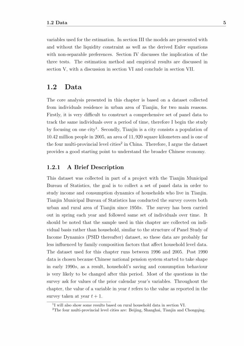
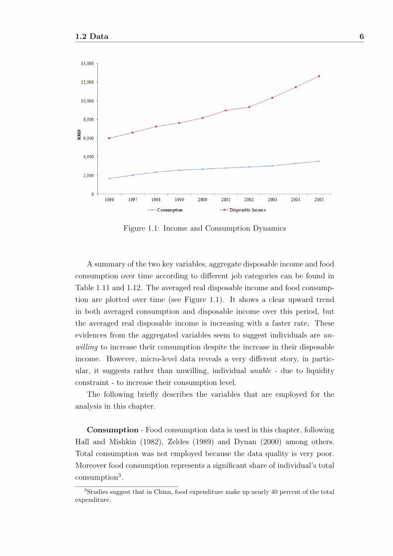
Figure 1.1: Income and Consumption Dynamics
A summary of the two key variables, aggregate disposable income and food
consumption over time according to different job categories can be found in
Table 1.11 and 1.12. The averaged real disposable income and food consump-
tion are plotted over time (see Figure 1.1). It shows a clear upward trend
in both averaged consumption and disposable income over this period, but
the averaged real disposable income is increasing with a faster rate. These
evidences from the aggregated variables seem to suggest individuals are un-
willing to increase their consumption despite the increase in their disposable
income. However, micro-level data reveals a very different story, in partic-
ular, it suggests rather than unwilling, individual unable - due to liquidity
constraint - to increase their consumption level.
The following briefly describes the variables that are employed for the
analysis in this chapter.
Consumption - Food consumption data is used in this chapter, following
Hall and Mishkin (1982), Zeldes (1989) and Dynan (2000) among others.
Total consumption was not employed because the data quality is very poor.
Moreover food consumption represents a significant share of individual’s total
consumption3.
3Studies suggest that in China, food expenditure make up nearly 40 percent of the totalexpenditure.

1.2 Data 7
The question in the survey asks “How much do you spend on your food
at home and restaurants in an average week?”. Food consumption data is
very likely to be measured with error, as shown in Table 1.8, it has a very
large standard deviation. Fortunately, parameter estimates presented in the
following sections are consistent as long as the first difference of the log mea-
surement error of consumption is unrelated to the regressors used.
Real Disposable Income - Questions were asked about how much in-
come do you receive in a month on average during the interview. The nominal
disposable income is first calculated as total income minus taxes plus trans-
fers. This is then adjusted for inflation, that is, deflated to constant prices
using index numbers. The formula is real disposable income equals disposable
income times the base year index, divided by the current year index. This is
summarized in Table 1.9, where it shows the average income is 8, 833RMB,
with a standard deviation of 4, 534 reflects the poor quality of the data, some-
how expected.
Real after-Tax Interest Rate - This reflects the actual rate of interest
paid on capital sum after allowance for the effects of inflation, see Table 1.10.
In this chapter, it is assumed that only investment option for each individual
is to invest in a one year government bond4. As a result, each individual’s
return on capital will be the same and equal to the one-year bond rate, as
given by the People’s Bank of China.
Year Dummy - In order to capture the year and other un-controlled
effects, eight year dummy variables are introduced.
1.2.2 Splitting the Sample
The approach of splitting the sample of individuals into two groups - sepa-
rating individuals who are more likely to be liquidity constrained and those
are less likely to be constrained - is the key for estimation strategy in this
chapter. It allows the test of the PIH/LCH, moreover it creates a natural
experiment to identify the impact of liquidity constraint. In particular, for
group one where each household’s current period liquidity constraint is not
binding implies the Lagrange multiplier corresponding to the constraint is zero
i.e. λi,t = 0, whereas for constrained group a positive Lagrange multiplier is
4Although it is not a realistic assumption, since household faces a shortage of investableassets in most emerging economies this assumption is not far from the reality.

1.3 The Model 8
expected. The sample is split by observations, so that a given individual can
sometimes fall in group one and other times in group two.
The sample is split into two groups according to different job categories,
because it is expected that nature of an individual’s job will have a major
impact on the likelihood to be liquidity constrained (see also Carroll and
Lawrence (1989)). The idea is that individuals who fall into the low ‘paid’
group will have less current-period disposable income, less assets and lower
savings to use as a buffer stock, however a steeper earning curve. Hence they
will have higher willingness, but more constrained (unable) to borrow. Out
of the 1500 people sampled, there are 50 professors, 100 government employ-
ees, 120 engineers, 130 school teachers, 300 people work in service sector and
finally 800 blue collar workers.
50 professors, 100 government employees, 120 engineers, 130 school teach-
ers and 300 people work in service sector (sales) are assigned to the first group,
who are less likely (relative to the second group) to be liquidity constrained.
The remaining 800 blue collar workers form the more liquidity constrained
group two. After this split there are 700 cross sectional observations in group
one and 800 in group two, which provides a well balanced sample size in each
group.
1.3 The Model
The Euler equation approach to test the PIH/LCH model under rational ex-
pectations was first developed by Hall (1978) and extended by Mankiw (1981),
Hansen and Singleton (1983) and others. Here the habit formation model is
presented with no liquidity constraints and with the corresponding set of Eu-
ler equations. In the second subsection, the model presented includes liquid-
ity constraints and derives the corresponding set of Euler equations. Zeldes
(1989) first applied this method using PSID data, so this chapter adopts the
estimation idea developed by Zeldes (1989) but the Euler equation used in this
chapter follows Hayashi (1985) and Dynan (2000). The goal of this section
is to extend the applicability of a PIH/LCH model to a developing country,
moreover, to understand the role of liquidity constraint in shaping Chinese
households’ consumption decisions.
1.3 The Model 9
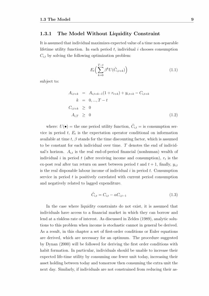
1.3.1 The Model Without Liquidity Constraint
It is assumed that individual maximizes expected value of a time non-separable
lifetime utility function. In each period t, individual i chooses consumption
Ci,t by solving the following optimization problem:
Et
( T−t∑k=0
βkU(Ci,t+k))
(1.1)
subject to:
Ai,t+k = Ai,t+k−1(1 + rt+k) + yi,t+k − Ci,t+kk = 0, ..., T − t
Ci,t+k ≥ 0
Ai,T ≥ 0 (1.2)
where: U(•) = the one period utility function, Ci,t = is consumption ser-
vice in period t, Et is the expectation operator conditional on information
available at time t, β stands for the time discounting factor, which is assumed
to be constant for each individual over time. T denotes the end of individ-
ual’s horizon. Ai,t is the real end-of-period financial (nonhuman) wealth of
individual i in period t (after receiving income and consumption), rt is the
ex-post real after tax return on asset between period t and t + 1, finally, yi,t
is the real disposable labour income of individual i in period t. Consumption
service in period t is positively correlated with current period consumption
and negatively related to lagged expenditure.
Ci,t = Ci,t − αCi,t−1 (1.3)
In the case where liquidity constraints do not exist, it is assumed that
individuals have access to a financial market in which they can borrow and
lend at a riskless rate of interest. As discussed in Zeldes (1989), analytic solu-
tions to this problem when income is stochastic cannot in general be derived.
As a result, in this chapter a set of first-order conditions or Euler equations
are derived, which are necessary for an optimum. The procedure suggested
by Dynan (2000) will be followed for deriving the first order conditions with
habit formation. In particular, individuals should be unable to increase their
expected life-time utility by consuming one fewer unit today, increasing their
asset holding between today and tomorrow then consuming the extra unit the
next day. Similarly, if individuals are not constrained from reducing their as-

1.3 The Model 10
set at the current amount, then they should not be able to increase expected
utility by consuming an extra unit today, decreasing holding, and reducing
consumption next period. The first order condition for each individual opti-
mization problem is:
Et
(MUi,t − αβMUi,t+1
)= Et
((1 + rt+1)βMUi,t+1 − (1 + rt+1)αβ2MUi,t+2
)(1.4)
where: MUi,t =δU(Ci,t)
δCi,trepresents the partial derivative of current utility with
respect to current consumption.
The left hand side of Equation 1.4 is the net marginal cost of forgoing one
unit of consumption expenditure in period t. The utility in period t decreases
and utility in the following period increases because habit stock in t + 1 is
lower. The right hand side represents next marginal benefits of increasing con-
sumption expenditure by (1+rt+1) units in period t+1. Where habit stock is
higher, the utility in period t+1 increases and utility in period t+2 decreases.
Equation 1.4 is simplified for the purposes of empirical estimation. One
reason for this is that there are only a limited number of observations available
for empirical estimations. More important, the methodologies suggested by
Zeldes (1989) are designed for linear equations, so the model needs to be
linearized. Hayashi (1985) provides a simplification of the first order condition
when preferences are time non-separable. If the time dimension T is large and
interest rate is constant, Equation 1.4 can be reduced to:
Et
((1 + r)β
MUi,t+1
MUi,t
)= 1 (1.5)
Under the assumption of rational expectations, Equation 1.5 implies:
(1 + r)β(MUi,t+1
MUi,t
)= 1 + ei,t (1.6)
where ei,t is individual i′s error uncorrelated with the information available
at time t, which reflects innovations to permanent income.
1.3.2 The Model With Liquidity Constraint
Under a general equilibrium setting, Scheinkman and Weiss (1986) show that
imposing exogenous restriction that individuals unable to borrow against the
future proceeds of their labour can induce price and output fluctuations that

1.3 The Model 11
mimic actual business cycles, but that are absent under a perfect markets
assumption. The importance of liquidity constraint is tested in this chapter
in the context of PIH/LCH, in order to shed some light on the overall Chinese
consumption level.
Many different forms of liquidity constraint have been examined in the
literature, to be consistent with the theme of this thesis, the constraint used
in this chapter is a floor on the total end-of-period net stock of traded asset
and it is not endogenously determined5. This kind of constraint has also been
used extensively in the literature, for example Bewley (1977), Scheinkman and
Weiss (1986) and Ljungqvist and Sargent (2004) among others. The equation
below constitutes what I refer to as a borrowing constraint throughout this
chapter:
Ai,t+k ≥ 0 (1.7)
Although liquidity constraint is a bigger set contains the borrowing constraint
defined here, I use the terms interchangeably in this chapter6. This constraint
implies that individual will have non-negative real end-of-period financial
wealth in period t, in other words, individuals can not consume today the
proceeds from supplying labour in the future.
The two hypothesis essentially differ by the fact that, under the null agents
can borrow and lend at the same rate, whereas the alternative hypothesis
‘restricts’ (liquidity constrained) individual to borrow from the market. Al-
though under the alternative hypothesis that all individuals face a set of
constraints at any point in time. Each individual could potentially build up
enough wealth in their early periods to relax these constraints, given China is
a developing country with low per capita incomes there will be periods where
some individuals hit the liquidity constraint. Therefore when the maximiza-
tion for this problem with the liquidity is derived, there will be a Lagrange
multiplier assigned to the constraint. Since the liquidity constraint is just
restricting individuals to borrow against their future wealth, while not being
5Essentially, the liquidity constraint can arise from financial market underdevelopmentor policy distortions. However, the constraint can also be interpreted as it is too expensivefor household to borrow.
6The constraint can be written in a more general form, for example Ai,t+k ≥ −B; k =0, ..., T − t − 1 where B is the limit on net indebtedness. In Chapter 2, I consider aslightly more general version of the constraint. Moreover, rather than considering exogenousquantity constrains, it would be interesting to study other reasons, such as credit historyand lenders’ credit supply conditions which can also lead to sub-optimal lending. Chen andVera (2012) look into this question using a UK dataset.

1.4 Description of the Euler Equation Test 12
restricted for saving. As a result, the Lagrange multiplier is expected to have
a positive sign, because if individuals are constrained with regard to borrow
by allowing them to borrow one more unit today, this should lead to a positive
increase in their lifetime utility - otherwise they would not choose to do so.
The ‘constrained’ version of the Euler equation is shown below:
MUi,t = Et((1 + r)βMUi,t+1) + λ′′
i,t (1.8)
where λ′′i,t is the Lagrange multiplier associated with the liquidity con-
straint7. For simplicity, I normalized the Lagrange multiplier, define λ′i,t:
λ′
i,t ≡λ′′i,t
Et((1 + r)βMUi,t+1)(1.9)
The Euler equation can be re-written as:
Et
((1 + r)β
MUi,t+1
MUi,t
)(1 + λ
′
i,t) = 1 (1.10)
Again by rational expectations, the equation above translates to:
(1 + λ′
i,t)(1 + r)βMUi,t+1
MUi,t= 1 + e
′
i,t (1.11)
where e′i,t is the error term.
1.4 Description of the Euler Equation Test
This chapter tests the null hypothesis that individuals are unconstrained
PIH/LCH consumers against the alternative hypothesis that individuals are
maximizing lifetime utility subject to a liquidity/borrowing constraint.
All tests in the rest of this chapter are based on the implication that a
current binding liquidity constraint will result in a violation of the Euler equa-
tion. Hereinafter, it is said that liquidity constraint is binding meaning that
individuals are constrained to borrow against their future assets/income and
this situation implies that the Lagrange multiplier associated with the liq-
uidity constraint is strictly positive and that furthermore, the Euler equation
between today and tomorrow is not satisfied.
7Scaled by a constant term.

1.4 Description of the Euler Equation Test 13
In order to estimate the Euler equation, some assumptions are made about
the preferences together with some additional identification assumptions.
1.4.1 Assumptions and Identification Issues
The utility function exhibits habit formation, in particular current utility
depends not only on today’s expenditures, but also on habit stock formed by
lagged expenditures. I assume the utility function is of the constant relative
risk aversion form
U(Ci,t) =(Ci,t)
1−ρ
1− ρ(1.12)
where ρ stands for the coefficient of risk aversion, assumed to be constant for
each individual and Ci,t stands for consumption services in current period,
which is positively related to current consumption and negatively related to
lagged expenditure.
Ci,t = Ci,t − αCi,t−1 (1.13)
The parameter α measures the strength of the habit formation, when
α is large, the consumer receives less lifetime utility from a given amount
of consumption, if α = 0 then the utility function is in the same form as
Zeldes (1989)8. The utility function can be substituted into Equation 1.11
and rearranged into the following form:
(1 + r)(1 + λ′
i,t)β( Ci,t
Ci,t−1
)−ρ= 1 + e
′
i,t (1.14)
Taking natural logarithm of the equation above and using Equation 1.13 to
substitute for C leads to:
∆ln(Ci,t − αCi,t−1) =1
ρ(ln(1 + r) + lnβ) +
1
ρln(1 + λ
′
i,t)−1
ρ(1 + e′i,t) (1.15)
Following Muellbauer (1988), I approximate ∆ln(Ci,t−αCi,t−1) by (∆lnCi,t−α∆lnCi,t−1) so Equation 1.15 can be rewritten as:
∆ln(Ci,t) = γ0 + α∆ln(Ci,t−1) + ε′
i,t + ln(1 + λi,t) (1.16)
For simplicity, λ′i,t is normalized with a sign preserving transformation i.e.
(1 + λi,t) ≡ (1 + λ′i,t)1ρ . Where γ0 is a constant term, moreover, it is a func-
tion of the real interest rate, the time discounting factor and forecast error
8without the taste preference parameters

1.4 Description of the Euler Equation Test 14
variance, but this chapter assumes that these terms are constant across house-
holds and different time periods and ε′i,t is the error term with mean zero.
As described above, the empirical tests use data on food consumption
rather than total consumption. Moreover, I do not consider the role for labour
supply or the purchase of durable goods. Therefore, I assume that the utility
function is additively separable in food, leisure, and other consumption goods.
Otherwise, additional terms will create extra variables in the Euler equation
and these data do not exist in the current survey.
1.4.2 Implication and Test I - Euler Equation Estima-
tion on the Two Groups
This chapter follows Zeldes (1989) and Runkle (1991) for the first test, which
suggest that the Euler equation is expected to be satisfied for group one but
not for group two. For this type of model it is necessary to test whether the
information known at time t is orthogonal to the error term. The standard
orthogonal test is carried out here by including lagged log of real disposable
income growth (ln(yi,t−1/yi,t−2)) in Equation 1.16, and test statistical sig-
nificance of this term in the regression. While in Zeldes (1987) log of real
disposable income is used, there is a concern that this term is correlated with
the expectation error term, because as mentioned earlier, if the current period
aggregate income were unexpectedly high, all individuals will have unexpected
higher consumption growth between current and last period, and higher ag-
gregate income means that each individual has higher income at macro level.
Furthermore, I have included eight extra dummy variables on the right hand
side of Equation 1.16 to capture the year effects of the data. So the equation
used for empirical estimation has the following specification:
ln(Ci,tCi,t−1
) = γ0 + αln(Ci,t−1
Ci,t−2
) + γ1ln(yi,t−1
yi,t−2
) +∑k
dkY Dki,t + εi,t + ln(1 + λi,t)
(1.17)
Equation 1.17 is estimated separately for each of the two groups. Under
the null hypothesis that liquidity constraint does not exist, λi,t will equal to
zero for both groups, implies that the parameter estimates should be plau-
sible and similar to each other, in particular, income should be insignificant
in explaining consumption in both cases. Under the alternative hypothesis
that liquidity constraint exists, empirical estimates based on group two data
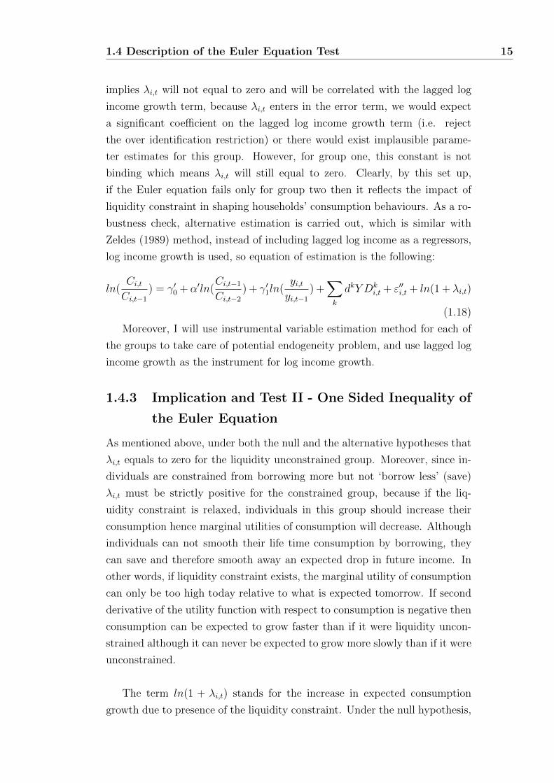
1.4 Description of the Euler Equation Test 15
implies λi,t will not equal to zero and will be correlated with the lagged log
income growth term, because λi,t enters in the error term, we would expect
a significant coefficient on the lagged log income growth term (i.e. reject
the over identification restriction) or there would exist implausible parame-
ter estimates for this group. However, for group one, this constant is not
binding which means λi,t will still equal to zero. Clearly, by this set up,
if the Euler equation fails only for group two then it reflects the impact of
liquidity constraint in shaping households’ consumption behaviours. As a ro-
bustness check, alternative estimation is carried out, which is similar with
Zeldes (1989) method, instead of including lagged log income as a regressors,
log income growth is used, so equation of estimation is the following:
ln(Ci,tCi,t−1
) = γ′0 + α′ln(Ci,t−1
Ci,t−2
) + γ′1ln(yi,tyi,t−1
) +∑k
dkY Dki,t + ε′′i,t + ln(1 + λi,t)
(1.18)
Moreover, I will use instrumental variable estimation method for each of
the groups to take care of potential endogeneity problem, and use lagged log
income growth as the instrument for log income growth.
1.4.3 Implication and Test II - One Sided Inequality of
the Euler Equation
As mentioned above, under both the null and the alternative hypotheses that
λi,t equals to zero for the liquidity unconstrained group. Moreover, since in-
dividuals are constrained from borrowing more but not ‘borrow less’ (save)
λi,t must be strictly positive for the constrained group, because if the liq-
uidity constraint is relaxed, individuals in this group should increase their
consumption hence marginal utilities of consumption will decrease. Although
individuals can not smooth their life time consumption by borrowing, they
can save and therefore smooth away an expected drop in future income. In
other words, if liquidity constraint exists, the marginal utility of consumption
can only be too high today relative to what is expected tomorrow. If second
derivative of the utility function with respect to consumption is negative then
consumption can be expected to grow faster than if it were liquidity uncon-
strained although it can never be expected to grow more slowly than if it were
unconstrained.
The term ln(1 + λi,t) stands for the increase in expected consumption
growth due to presence of the liquidity constraint. Under the null hypothesis,

1.4 Description of the Euler Equation Test 16
this term is equal to zero for both groups and the parameter estimates should
be similar, however, under the alternative hypothesis this term remains zero
for group one and if group two observations are not liquidity constrained then
this term should be statistically insignificant from zero. To estimate this term,
Equation 1.17 will be estimated (without λi,t included) for group one. If the
liquidity constraint is not binding for group two, then these parameter esti-
mates will be also consistent estimates for group two. I then use the group
one parameter estimates to construct estimates of group two residuals xi,t,
letting the estimated residual be labeled xi,t.
The estimated residual xi,t in Equation 1.17 includes both the Lagrange
multiplier term and the disturbance εi,t term. However the εi,t term has
a mean of zero, hence sample mean of xi,t over all observations in group
two will equal to the sample mean of the Lagrange multiplier (call this ¯xi,t).
Furthermore, as size of cross sectional observation N goes to infinity sample
mean of xi,t will approach to the population mean. So ¯xi,t will be a consistent
estimate of the group two population mean of ln(1+λi,t). In turn, this means
that if the liquidity constraint is binding for the second group, this estimate
should be statistically significant different from zero, more specifically, strictly
positive.
1.4.4 Implication and Test III - The Relationship be-
tween λi,t and yi,t
For individuals in group two, if their real disposable income increase at time
t and all other variables are kept constant, this situation will directly relax
their liquidity constraints, consumption should increase today (relative to
tomorrow) hence λi,t will fall. Therefore, under the existence of liquidity
constraint, there should be a negative partial correlation between λi,t and yi,t
(since yi,t is assumed to be uncorrelated with the error term). As a test of
this, the estimate xi,t is regressed on yi,t. The sign will then be tested to see
if it is negative. However this is an estimate for the total derivate which may
not necessarily be the same as partial derivative.
1.5 Empirical Analysis and Results 17
1.5 Empirical Analysis and Results
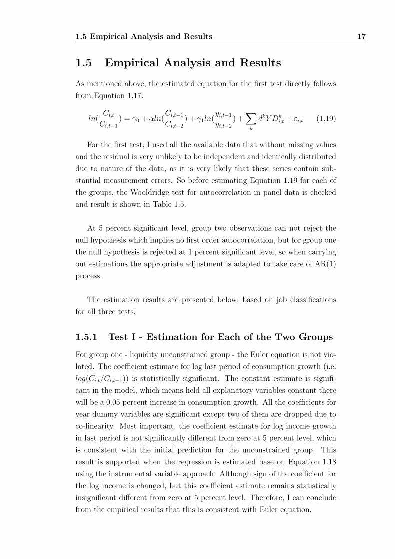
As mentioned above, the estimated equation for the first test directly follows
from Equation 1.17:
ln(Ci,tCi,t−1
) = γ0 + αln(Ci,t−1
Ci,t−2
) + γ1ln(yi,t−1
yi,t−2
) +∑k
dkY Dki,t + εi,t (1.19)
For the first test, I used all the available data that without missing values
and the residual is very unlikely to be independent and identically distributed
due to nature of the data, as it is very likely that these series contain sub-
stantial measurement errors. So before estimating Equation 1.19 for each of
the groups, the Wooldridge test for autocorrelation in panel data is checked
and result is shown in Table 1.5.
At 5 percent significant level, group two observations can not reject the
null hypothesis which implies no first order autocorrelation, but for group one
the null hypothesis is rejected at 1 percent significant level, so when carrying
out estimations the appropriate adjustment is adapted to take care of AR(1)
process.
The estimation results are presented below, based on job classifications
for all three tests.
1.5.1 Test I - Estimation for Each of the Two Groups
For group one - liquidity unconstrained group - the Euler equation is not vio-
lated. The coefficient estimate for log last period of consumption growth (i.e.
log(Ci,t/Ci,t−1)) is statistically significant. The constant estimate is signifi-
cant in the model, which means held all explanatory variables constant there
will be a 0.05 percent increase in consumption growth. All the coefficients for
year dummy variables are significant except two of them are dropped due to
co-linearity. Most important, the coefficient estimate for log income growth
in last period is not significantly different from zero at 5 percent level, which
is consistent with the initial prediction for the unconstrained group. This
result is supported when the regression is estimated base on Equation 1.18
using the instrumental variable approach. Although sign of the coefficient for
the log income is changed, but this coefficient estimate remains statistically
insignificant different from zero at 5 percent level. Therefore, I can conclude
from the empirical results that this is consistent with Euler equation.

1.5 Empirical Analysis and Results 18
For group two, the coefficient estimate for consumption growth in the
previous period and the constant estimate are almost identical and both are
statistically significant compared to the group one estimates. However, the
coefficient for the lagged log income growth is negative, and its magnitude
is nearly twice as large as the coefficient estimate for group one, most im-
portantly this coefficient is significantly different from zero at 5 percent level.
Again, this evidence is supported when the parameter is estimated using
Equation 1.18 and the coefficient for log income growth last period is sig-
nificantly different from zero at 1 percent level, which is a stronger result.
As discussed before, this is inconsistent with the PIH/LCH and this is the
prediction under the existence of liquidity constraint. Moreover estimated
coefficients for year dummies are all significant apart from the dummy for
year 1998, which has been dropped due to co-linearity.
Table 1.1: Test I: Euler Equation for Two Samples
Dependent Variable: log(Ci,tCi,t−1
)
Independent Variables Group 1 Group 2
Constant 0.0482*** 0.0477***(0.002) (0.002)
log(Ci,t−1
Ci,t−2) -0.5551*** -0.5374***
(0.013) (0.013)log(
yi,t−1
yi,t−2) 0.0261 -0.0396**
(0.035) (0.020)year dummies yes yes
Number of observations 4884 5587N 698 799
Robust standard errors in parentheses. ∗ ∗ ∗p < 0.01, ∗ ∗ p < 0.05, ∗p < 0.1
To summarize, these results (see Table 1.1 and 1.6) show that the PIH/LCH
have significant power in explaining consumption behavior of the Chinese
household, moreover, the inability to pledge against future income forces
the liquidity constrained household to deviate from a smoothed consumption
path.
1.5.2 Test II - One-side Inequality in the Euler Equa-
tion
In Table 1.2, I present a consistent estimate for the averaged Lagrange mul-
tiplier from group two sample which equals to the averaged unexplained con-
sumption growth in this group. It was expected that this term should be
strictly positive for the constrained group two. The Portmanteau test for

1.5 Empirical Analysis and Results 19
white noise is carried out for the sequence of xi,t. Since the sample size is
relatively large, the central limit theorem implies that xi,t should be white
noise. Table 1.7 shows rejection of the Portmanteau test, which suggests this
sequence is not white noise. The point estimate for the averaged Lagrange
multiplier is 0.010. Moreover, this averaged Lagrange multiplier is signifi-
cantly greater than zero at 1 percent level (one tail test) because the sample
mean should follow a normal distribution with a mean of 0.01 and a variance
of 0.051/n (n=sample size).
Table 1.2: Test II: Estimate of Average Excess Consumption Growth
Group Two due to Binding Liquidity Constraint
¯xi,t 0.0095229***(0.051)
Robust standard errors in parentheses. ∗ ∗ ∗p < 0.01, ∗ ∗ p < 0.05, ∗p < 0.1
Furthermore, the histogram plotted in Figure 1.4 confirms these error
terms are not only statistically different from zero, but greater than zero on
average. In particular, Figure 1.4 shows most of the estimated ‘errors’ are
indeed lying on the positive region. The estimate is more statistically sig-
nificant compare to the one in Zeldes (1989), which is consistent with the
expectation that Chinese households are more liquidity constrained relative
to household in US. The possible reasons behind the underdevelopment of
Chinese financial markets are being explored in the second and third chapter
of this thesis.
So far, the first test leads to a rejection of the Euler equation for liquid-
ity constrained group but not for group one. The second test indicates that
sign and magnitude of the one-sided inequality are consistent with the view
that liquidity constraints exist and have a major impact on individual’s con-
sumption behaviour in particular liquidity constrained households consume
less than they would otherwise have done.
1.5.3 Test III - Relationship between Unexplained Con-
sumption Growth and Income
The results from regressing xi,t on the log of real disposable income (ln(yi,t))
is shown in Table 1.3. The estimated coefficient for the log of real disposable
income is negative, more important it is statistically significant at 5 percent
level. The coefficient is a consistent estimate of the relationship between the

1.6 Discussion 20
Lagrange multiplier and current income, it suggests that individuals in group
two are facing a binding borrowing constraint. It is negative, meaning that if
disposable income at time t increases and nothing else in the model changes,
the constraint will be relaxed directly, hence the Lagrange multiplier will fall.
Table 1.3: Test III: Regression of Estimate of Excess Consumption Growth
Group Two on the log of Real Disposable Income
ln(yi,t) -0.0913**(0.008)
Robust standard errors in parentheses. ∗ ∗ ∗p < 0.01, ∗ ∗ p < 0.05, ∗p < 0.1
1.6 Discussion
1.6.1 Evidence on Habit Formation
So far the discussion has focused on impact of liquidity constraint on house-
holds’ consumption behaviors. Since the utility function exhibits habit for-
mation, whether Chinese household’s consumption behaviour has been influ-
enced by habit formation can be studied using the estimation results based
on liquidity unconstrained (group one) sample. The habit formation model
predicts α in Equation 1.16 to be strictly positive, with its magnitude re-
flecting the fraction of past expenditures that make up the habit stock and
indicating the importance of habit formation in behavior. Intuitively, Equa-
tion 1.16 shows that habit formation creates a positive link between current
and lagged consumption growth, which stems from consumers’ gradual ad-
justment to permanent income shocks. In contrast to traditional models in
which consumption adjusts immediately to permanent income innovations,
habits cause consumers to prefer a number of small consumption changes to
one large consumption change. Results in Table 1.1 shows that the coefficient
estimate for α is −0.56, thus, there is no evidence of significant habit forma-
tion in food consumption.
Some caveats apply in making the conclusion, for example durability in
the data could partially or even completely obscure habit formation. Durabil-
ity tends to offset habit formation in behaviour, it makes expenditure growth
lumpy whereas habit smooth it out. Hayashi (1985) shows that with durability
alone, α should be negative. The variable of interest in this chapter is annual
food consumption, therefore it is very unlikely to be durable. However, the re-

1.6 Discussion 21
sults hinge on the assumption that preferences are separable in food and other
expenditures, if food were a complement to other expenditures, the durability
of related goods might affect the dynamics of food spending. Unfortunately,
it is impossible to study separate habit formation and durability parameters
with the current dataset and it is not the main focus of current chapter.
1.6.2 An Alternative ‘Story’ on Aggregate Chinese Con-
sumption
As the results based on group two observations show, if additional resource
can be obtained, for example by allowing household to borrow against fu-
ture income or increase low income bracket households’ disposable income,
liquidity constrained households will respond by increasing current period
consumption, whereas the effect is silent for the unconstrained group. This
result provides an alternative story in explaining the low consumption level
(as share of GDP) in China - suppose that liquidity constrained households
have a ‘desired’ level of consumption (implied by the PIH/LCH) over their
lifetime, moreover they expect their future income will grow at a rate in line
with the rate which the aggregate economy grows. Now during early period
of their life time, they would have borrowed to smooth their consumption,
in particular, they borrow against expected (higher) future income, to in-
crease current period consumption. However, due to the existence of liquidity
constraint they can only consume what their current period income allows.
Whereas in the later part of life time (before retirement), their incomes eas-
ily exceed the cost of ‘desire’ level of consumption therefore they will save
the remaining incomes. This story predicts that the low consumption level,
moreover the high saving rates in China will automatically correct itself as
the financial market develops and household’s income grows (evenly across
different income brackets) in China. Moreover, it suggests the policy focus
should be steered away from the conventional views, on to financial market
development and increase household’s income.
Unfortunately this hypothesis is not tested in this chapter due to data
limitation, however, in the next subsection I discuss some findings from the
rural area in China does also support this argument.

1.6 Discussion 22
1.6.3 Some Evidence from the Rural Household
Rural household represents a large share of the total population in China, al-
though this share has fallen from over 70 percent during 1990s to 50 percent
by 2010, it still represents nearly 7bn people. The ratio between averaged
rural household net income to urban household disposable income has fallen
from 45 percent in 1990 to 31 percent in 2010. Moreover, the price index
for rural residence grown at a similar rate as the urban price index, while
the rate of rural household income increased has not been able to match up
with the urban counter part. Therefore, it is natural to expect that the rural
households are more liquidity constrained relative to the urban households,
put it differently, if liquidity constraint or even precautionary saving motives
(as argued in the literature as the main factor drives the high saving rate in
China) have any effects on the Chinese household consumption and saving
decisions, they should have larger impact on the rural household.
To my knowledge, very few analysis using Chinese rural household data
exist in the literature, the main reason was due to data availability, unfortu-
nately, I do not escape from this problem. It is very difficult to track same
set of individuals over a period of time to construct a similar panel in rural
China. Therefore in this subsection I try to provide some evidences based
on a country-wide dataset which reveal three key findings: 1, liquidity con-
straint has a significant impact in shaping household consumption behaviours
in rural area; 2, similar to my previous findings, liquidity constraint affects
the low income bracket households the most. Moreover, the analysis sug-
gests that the bottom 40 percent of the rural household are unable to save,
in other words, it is the households in top income brackets, after meeting
their ‘desired’ level of consumption, depositing the ‘extra’ incomes (due to
lack of investment opportunities, the extra income is usually packed at bank
deposit.) and contributing to the high aggregate saving rate in China. This
is particularly interesting, because if this finding is robust, then policy inter-
ventions such as improving the social safety nets will not necessary have a big
impact on boosting Chinese consumption level or lowering the saving rate in
China9. Instead, policy designed to boost low income households’ wage will
be a more efficient way to increase consumption level, policy designed to im-
prove financial market structure - such as widening asset classes accepted as
collateral and improving credit worthiness assessment system - will be a more
9This does not imply the Chinese Government should not improve the social safety net,instead it says these policy will have little impact on resolving the ‘saving glut’.
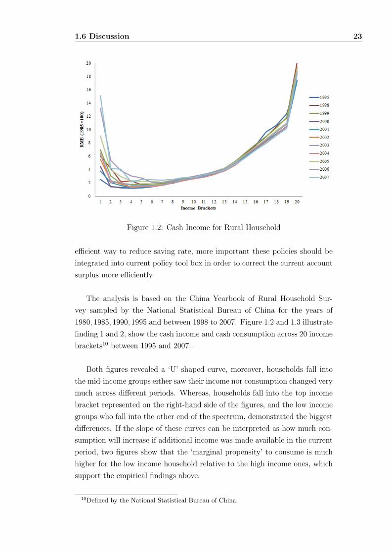
1.6 Discussion 23
Figure 1.2: Cash Income for Rural Household
efficient way to reduce saving rate, more important these policies should be
integrated into current policy tool box in order to correct the current account
surplus more efficiently.
The analysis is based on the China Yearbook of Rural Household Sur-
vey sampled by the National Statistical Bureau of China for the years of
1980, 1985, 1990, 1995 and between 1998 to 2007. Figure 1.2 and 1.3 illustrate
finding 1 and 2, show the cash income and cash consumption across 20 income
brackets10 between 1995 and 2007.
Both figures revealed a ‘U’ shaped curve, moreover, households fall into
the mid-income groups either saw their income nor consumption changed very
much across different periods. Whereas, households fall into the top income
bracket represented on the right-hand side of the figures, and the low income
groups who fall into the other end of the spectrum, demonstrated the biggest
differences. If the slope of these curves can be interpreted as how much con-
sumption will increase if additional income was made available in the current
period, two figures show that the ‘marginal propensity’ to consume is much
higher for the low income household relative to the high income ones, which
support the empirical findings above.
10Defined by the National Statistical Bureau of China.

1.6 Discussion 24
Figure 1.3: Cash Consumption for Rural Household
Moreover, I constructed a simple measure (based on the data available)
tries to capture the idea of inability to save which reflects both the household’s
ability to save as well as to consume, defined as:
disposable income(cash) − (total income − cash income) − living
expenditure(cash)
The idea is that if this measure is below 0 implies in the current period
(year), the households on average (within this income bracket) will not have
sufficient cash income to finance their cash living expenditures11, as a result
they will not only be credit constrained to achieve the ‘desired’ (implied by
the PIH/LCH) level of consumption, but will not be able to save for example
making any bank deposit. The share of rural household who fall into this
category is listed in Table 1.4 for the years that data is available and I argue
this measure provide, at least, a lower bound of the share of rural household
who are unable to save.
These results suggest that on average 40 percent of the rural household
can not save, that is a quarter of the total Chinese population, on the other
hand household in the top income brackets, alone, is contributing to the high
saving rates in China.
11this shortfall is normally met using savings or interest payment.
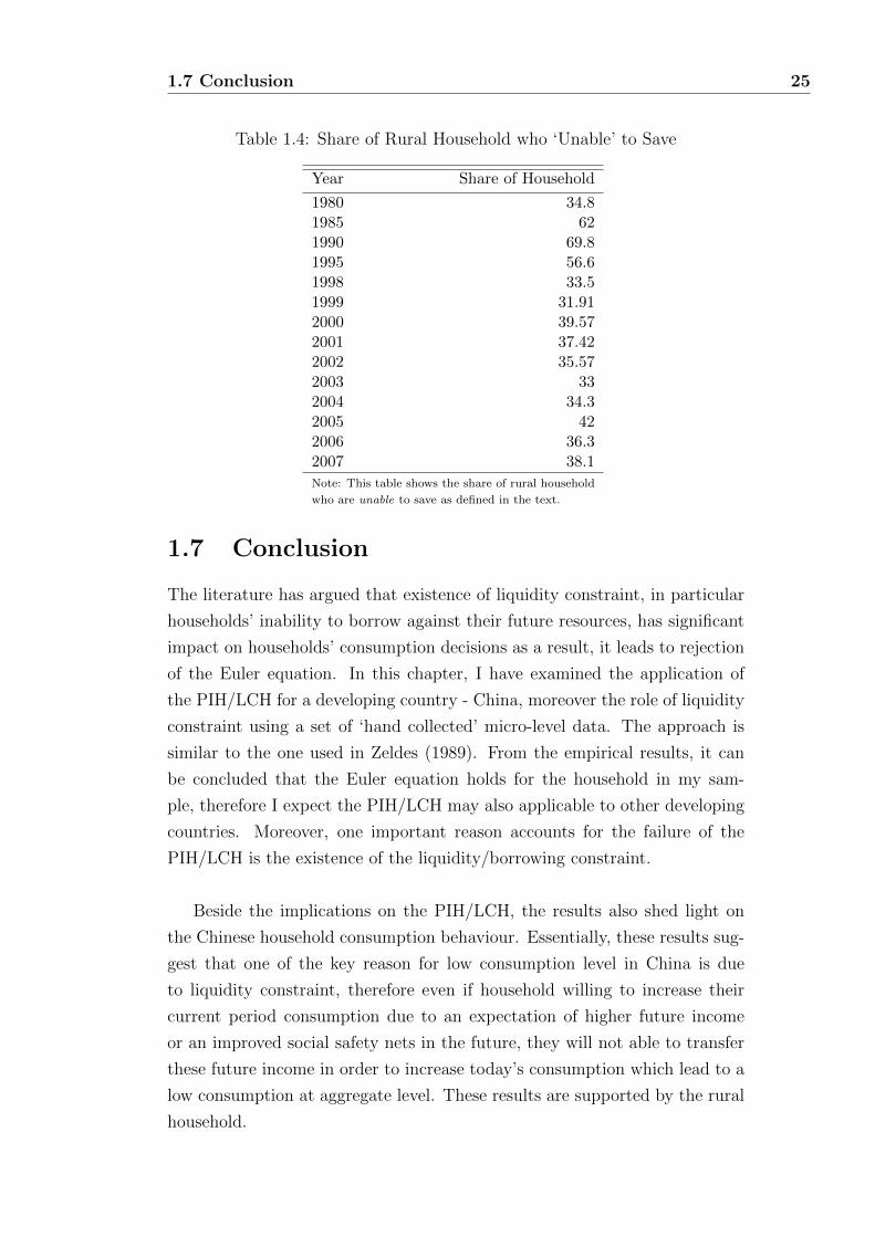
1.7 Conclusion 25
Table 1.4: Share of Rural Household who ‘Unable’ to Save
Year Share of Household
1980 34.81985 621990 69.81995 56.61998 33.51999 31.912000 39.572001 37.422002 35.572003 332004 34.32005 422006 36.32007 38.1
Note: This table shows the share of rural household
who are unable to save as defined in the text.
1.7 Conclusion
The literature has argued that existence of liquidity constraint, in particular
households’ inability to borrow against their future resources, has significant
impact on households’ consumption decisions as a result, it leads to rejection
of the Euler equation. In this chapter, I have examined the application of
the PIH/LCH for a developing country - China, moreover the role of liquidity
constraint using a set of ‘hand collected’ micro-level data. The approach is
similar to the one used in Zeldes (1989). From the empirical results, it can
be concluded that the Euler equation holds for the household in my sam-
ple, therefore I expect the PIH/LCH may also applicable to other developing
countries. Moreover, one important reason accounts for the failure of the
PIH/LCH is the existence of the liquidity/borrowing constraint.
Beside the implications on the PIH/LCH, the results also shed light on
the Chinese household consumption behaviour. Essentially, these results sug-
gest that one of the key reason for low consumption level in China is due
to liquidity constraint, therefore even if household willing to increase their
current period consumption due to an expectation of higher future income
or an improved social safety nets in the future, they will not able to transfer
these future income in order to increase today’s consumption which lead to a
low consumption at aggregate level. These results are supported by the rural
household.

1.7 Conclusion 26
However, these results should be interpreted with caution. The data con-
tains considerable measurement errors as well as less than ideal in that some
more variables need to be constructed. The model could be improved by
many ways, such as introducing bequest motive and a taste factor in the util-
ity function or including some demographic information of each individual
and some household information. Moreover, tests should be re-estimated us-
ing different ways of splitting the sample as a robustness check. I conclude
the main improvement is needed on the quality of data collection, which is
one of the tasks I am currently undertaking.
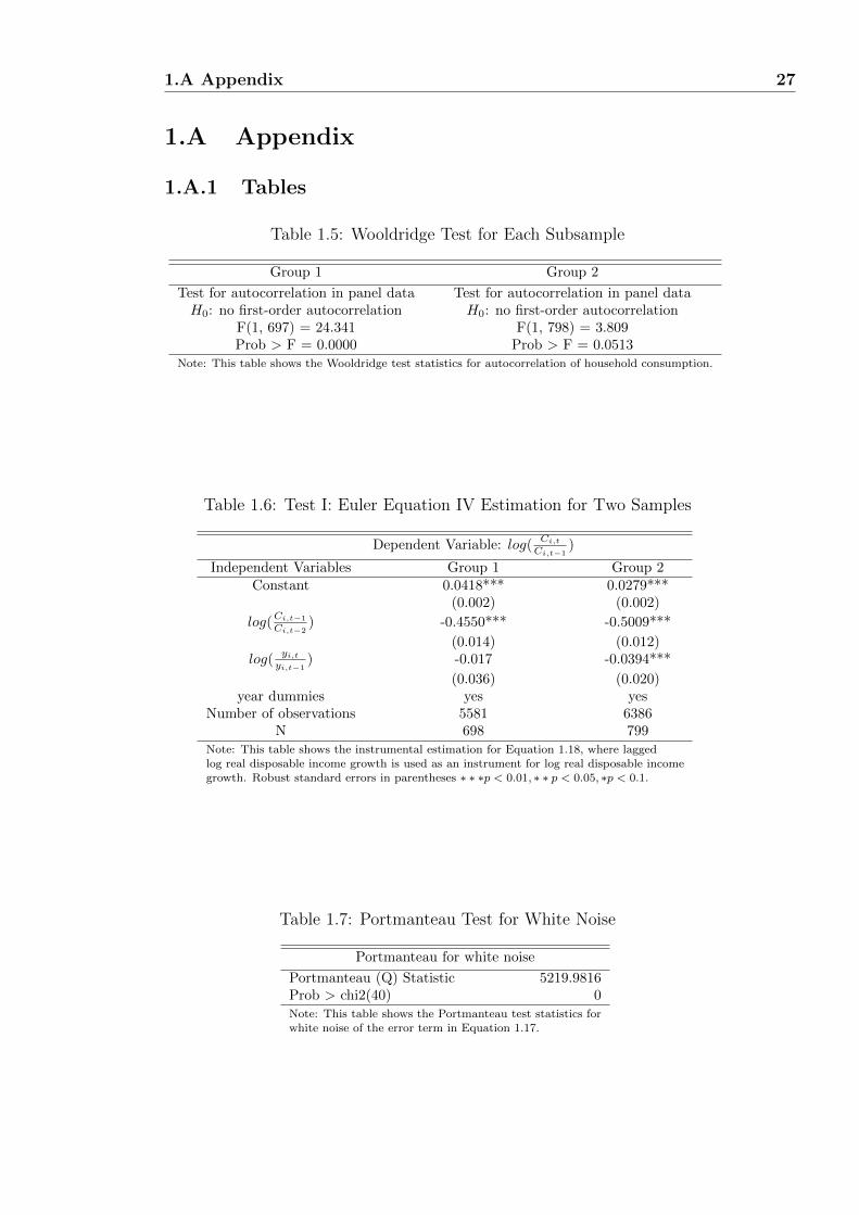
1.A Appendix 27
1.A Appendix
1.A.1 Tables
Table 1.5: Wooldridge Test for Each Subsample
Group 1 Group 2
Test for autocorrelation in panel data Test for autocorrelation in panel dataH0: no first-order autocorrelation H0: no first-order autocorrelation
F(1, 697) = 24.341 F(1, 798) = 3.809Prob > F = 0.0000 Prob > F = 0.0513
Note: This table shows the Wooldridge test statistics for autocorrelation of household consumption.
Table 1.6: Test I: Euler Equation IV Estimation for Two Samples
Dependent Variable: log(Ci,t
Ci,t−1)
Independent Variables Group 1 Group 2Constant 0.0418*** 0.0279***
(0.002) (0.002)
log(Ci,t−1
Ci,t−2) -0.4550*** -0.5009***
(0.014) (0.012)log(
yi,t
yi,t−1) -0.017 -0.0394***
(0.036) (0.020)year dummies yes yes
Number of observations 5581 6386N 698 799
Note: This table shows the instrumental estimation for Equation 1.18, where laggedlog real disposable income growth is used as an instrument for log real disposable incomegrowth. Robust standard errors in parentheses ∗ ∗ ∗p < 0.01, ∗ ∗ p < 0.05, ∗p < 0.1.
Table 1.7: Portmanteau Test for White Noise
Portmanteau for white noise
Portmanteau (Q) Statistic 5219.9816Prob > chi2(40) 0Note: This table shows the Portmanteau test statistics forwhite noise of the error term in Equation 1.17.

1.A Appendix 28
1.A.2 Figures
Figure 1.4: Histogram for the ‘Error’ Term

1.A Appendix 29
1.A.3 Data
Table 1.8: Descriptive Food Consumption Statistics
Variable Mean Std. Dev. Min Max Observations(RMB) (RMB) (RMB)
Food overall 2682.02 1369.961 172.1 19965.2 N = 14997
Consumption between 1199.6 1839.68 8591.53 n = 1500
within 662.1212 2927.97 17072.87 T-bar = 10
Note: This table shows some summary statistics of food consumption between 1996 and 2005for household resident in Tianjin.
Table 1.9: Descriptive Real Disposable Income Statistics
Variable Mean Std. Dev. Min Max Observations(RMB) (RMB) (RMB)
Real overall 8833.426 4534.746 522.1 36996.5 N = 14997
Disposable between 3929.88 6091.38 26108.82 n = 1500
Income within 2264.347 1354.174 20920.2 T-bar = 10
Note: This table shows some summary statistics of real disposable income between 1996 and 2005for household resident in Tianjin.
Table 1.10: Real Annual Interest Rate
Year Real Interest Rate
1996 9.181997 7.471998 5.671999 5.222000 4.772001 3.782002 2.252003 1.982004 2.252005 2.52
Note: This table shows the real interest rateone year government bond.

1.A Appendix 30
Table 1.11: Data Description I
Real Food Real FoodJob Sample disposable consumption disposable consumption
Classifications size income 1996 1996 income 1997 1997
Govt. Employee 100 1980010 555046 1796495 524559Engineer 120 2174390 609536 1972859 576056Professor 50 1796020 503469 1629558 475815Teacher 130 2207370 618781 2002782 584793Worker 800 7488010 2099075 6793992 1983780Sales 300 3312025 928443 3005054 877447
Total 1500 18957825 5314350 17200740 5022450Average 12638.55 3542.9 11467.16 3348.3
Real Food Real FoodJob Sample disposable consumption disposable consumption
Classifications size income 1998 1998 income 1999 1999
Govt. Employee 100 1615666 473346 1462859 456426Engineer 120 1774277 519815 1606470 501234Professor 50 1465531 429361 1326925 414013Teacher 130 1801188 527698 1630836 508836Worker 800 6110129 1790100 5532248 1726113Sales 300 2702574 791780 2446972 763478
Total 1500 15469365 4532100 14006310 4370100Average 10312.91 3021.4 9337.54 2913.4
Note: This table shows some summary statistics of real disposable income and food consumptionin RMB between 1996 and 1999 for household resident in Tianjin.
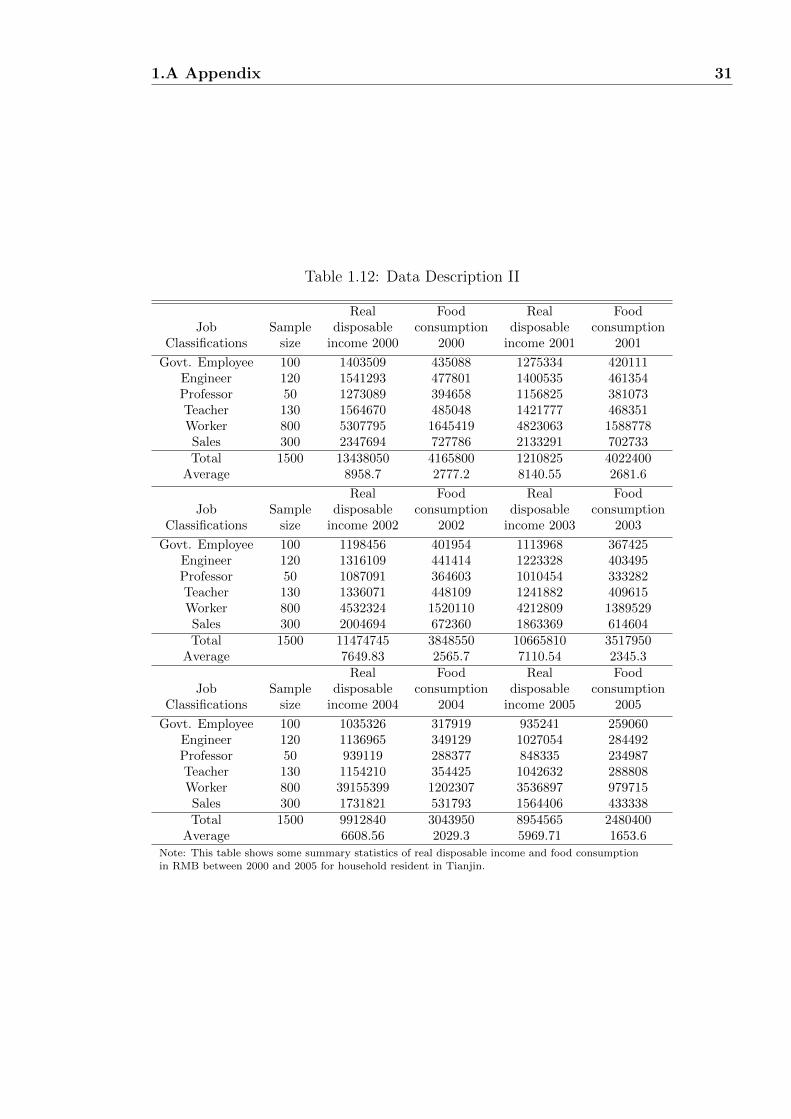
1.A Appendix 31
Table 1.12: Data Description II
Real Food Real FoodJob Sample disposable consumption disposable consumption
Classifications size income 2000 2000 income 2001 2001
Govt. Employee 100 1403509 435088 1275334 420111Engineer 120 1541293 477801 1400535 461354Professor 50 1273089 394658 1156825 381073Teacher 130 1564670 485048 1421777 468351Worker 800 5307795 1645419 4823063 1588778Sales 300 2347694 727786 2133291 702733Total 1500 13438050 4165800 1210825 4022400
Average 8958.7 2777.2 8140.55 2681.6
Real Food Real FoodJob Sample disposable consumption disposable consumption
Classifications size income 2002 2002 income 2003 2003
Govt. Employee 100 1198456 401954 1113968 367425Engineer 120 1316109 441414 1223328 403495Professor 50 1087091 364603 1010454 333282Teacher 130 1336071 448109 1241882 409615Worker 800 4532324 1520110 4212809 1389529Sales 300 2004694 672360 1863369 614604Total 1500 11474745 3848550 10665810 3517950
Average 7649.83 2565.7 7110.54 2345.3Real Food Real Food
Job Sample disposable consumption disposable consumptionClassifications size income 2004 2004 income 2005 2005
Govt. Employee 100 1035326 317919 935241 259060Engineer 120 1136965 349129 1027054 284492Professor 50 939119 288377 848335 234987Teacher 130 1154210 354425 1042632 288808Worker 800 39155399 1202307 3536897 979715Sales 300 1731821 531793 1564406 433338Total 1500 9912840 3043950 8954565 2480400
Average 6608.56 2029.3 5969.71 1653.6Note: This table shows some summary statistics of real disposable income and food consumptionin RMB between 2000 and 2005 for household resident in Tianjin.
Chapter 2
Firm Productivity and the
Current Account: One Country
with Two Financial Markets
2.1 Introduction
Three facts have dominated the discussion on the Chinese economy and global
macroeconomics:
Fact 1: The state-owned enterprises (SOEs) on average have lower pro-
ductivity level compare to privately-owned enterprises (POEs) in China (see
Figure 2.1).
Fact 2: The Chinese economy has run a persistent current account surplus
since the early 1990s; the counterparts of its surplus has been the deficit in
the United States, the United Kingdom and other advanced economies1(see
Figure 2.2).
Fact 3: The long run real interest rate has been declining over the last
decade (see Figure 2.3), despite recent efforts from central banks to raise in-
terest rates - The “Greenspan’s Conundrum”.
Despite extensive studies on various factors driving this environment, there
1India, a country which is at a similar stage of financial development as China (accordingto the Financial Freedom Index see Figure 2.12), has completely opposite ‘experiences’ incurrent account balance. The Indian story suggests that, it is difficult to explain China’scurrent account surplus by just focusing on the aggregate financial market development.
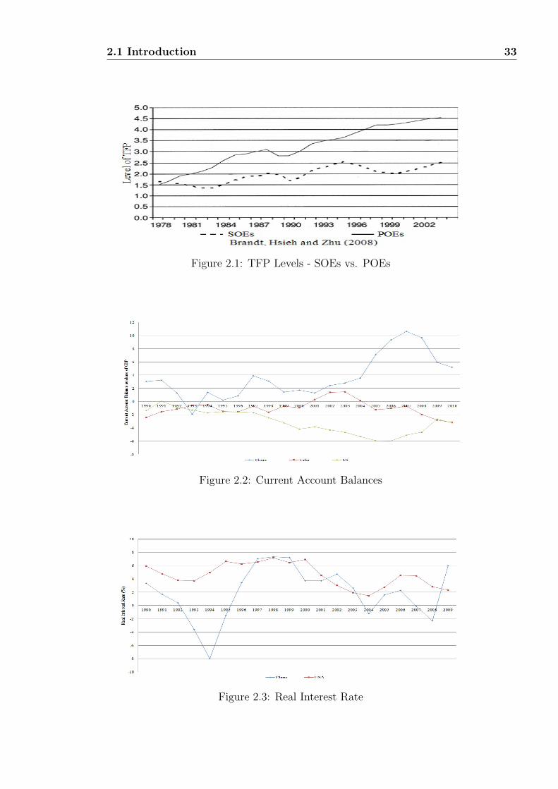
2.1 Introduction 33
Figure 2.1: TFP Levels - SOEs vs. POEs
Figure 2.2: Current Account Balances
Figure 2.3: Real Interest Rate
2.1 Introduction 34
are very few formal structures to analyze these joint phenomena. The growth
literature deals with fact 1 (Brandt, Hsieh, and Zhu (2008) and Brandt and
Zhu (2010)), while international macroeconomics deals with fact 2 and 3, al-
though these facts are deeply integrated in practice. In this chapter I argue
that such separation between the real economy and the financial market is
not warranted when the productivity differential in China is an important
driving force behind the last two set of facts. Hence it must be made an
integral part of analysis if we are to conjecture on what got the world into
the current situation and how it is likely to get out of it.
There have been many papers documented the productivity differential
between SOEs and POEs in China. Song, Storesletten, and Zilibotti (2011),
using the ratio between net fixed asset investment and total profit as a mea-
sure of productivity, show the productivity gap between SOEs and POEs is
about 9 percentage point per year, and a similar figure was reported by Islam,
Dai, and Sakamoto (2006). I confirm these results by comparing output to
total asset ratio between SOEs and POEs across 28 manufacturing industries
(see Figure 2.13). From the TFP accounting point of view, Brandt, Hsieh,
and Zhu (2008)) estimate an average TFP gap between POEs and SOEs of
1.8 during 1998− 2004, while Brandt and Zhu (2010) estimate a gap of 2.3 in
2004. Furthermore, using a different methodology, Hsieh and Klenow (2009)
estimate a “revenue-TFP” of 1.42.
A number of theories argue that the global imbalances is the product of
credit frictions in Emerging Markets (EMs) have emerged in recent years.
These papers focus on fact 2 or 3, while fact 1 is largely ignored. Caballero,
Farhi, and Gourinchas (2006) primarily analyze the collapse of asset markets
in newly industrialized economies (or EMs). Following a collapse in the asset
market, newly industrialized economies’ abilities to supply financial assets to
savers are reduced, so savings flow towards advanced economies in search of
investable assets, and long run interest rate declines. The key mechanism in
their paper, is a collapse in the asset market leads to a reduction in agents’
borrowing abilities, which transfer to a reduction in domestic asset supply
one to one. Moreover, both investments and outputs in newly industrial-
ized economy remain unaffected by the shock (ignoring fact 1). However,
financial frictions have proven to be one of the most important factors be-
hind both investment and economic development (see Jeong and Twonsend
(2005), Amaral and Quintin (2010), Buera, Kaboski, and Shin (2009), Moll

2.1 Introduction 35
(2010), Greenwood, Sanchez, and Wang (2010) and Midrigan and Xu (2010)).
In contrast, I explicitly model the impact of borrowing ability on investment
and output, via firm’s entry decision, which permits the interplay of both
saving and investment in determining capital flow. In this chapter, shock to
a firm’s borrowing ability affects its optimal entry decision. These decisions
collectively form the structure of the industry, in turn affect the equilibrium
productivity level, furthermore the new industrial composition will interact
with the financial shock shapes the new domestic saving and investment rates.
Coeurdacier, Guibaud, and Jin (2011) explain the high saving rates in EMs, as
a consequence of households in EMs have tighter liquidity constraints (relative
to households in Advanced Economies). However, liquidity constraint should
be a dynamic concept; by keeping it fixed the key picture will be missed.
Moreover, on the saving side, Mendoza, Quadrini, and Rios-Rull (2009) show
that lower risk sharing opportunities in developing countries increase precau-
tionary savings so that when opening up to capital markets, these countries
see a net capital outflows. However, risk is likely to be of second-order com-
pared to the rapid productivity growth in EMs. Some other papers have put
the emphasis on corporate savings. Sandri (2010) shows that in the face of
uninsurable investment risks, firms rely on precautionary savings to finance
future investment opportunities. Bacchetta and Benhima (2010) show that
credit-constrained firms in EMs demand liquidity to finance investment in
periods of high productivity growth with the assumption that demand for
foreign bond complements domestic investment when firms are credit con-
strained. In both papers, corporate savings rise above investment, and the
outcome is a net capital outflow, although it is unclear that corporate savings
are the force behind the current account imbalances. Bayoumi, Tong, and
Wei (2010) using firm-level data, show that corporate saving rate has fallen
in China; furthermore, Chinese firms do not have a significantly higher sav-
ing rate than the global average. It is the household’s counterpart in China,
however is much higher compares to advanced economies.
On the investment side, Buera and Shin (2010) emphasize a suppression
of investment demand due to financial frictions. While investment slowed
down during the East Asian crisis, it quickly reverted back to a beyond the
pre-crisis level in Emerging Asia, making investment a less plausible candi-
date for explaining the recent divergence in global imbalances. Furthermore,
Song, Storesletten, and Zilibotti (2011) provide a framework to explain some
facts during China’s economic transition. The key assumption in their paper

2.1 Introduction 36
is that, POEs are more productive relative to SOEs ex-ante, and the main
mechanism is that resources re-allocate to more productive POEs over the
transition, as a result the size of financially integrated SOEs shrink, and do-
mestic savings are stored in foreign assets. Essentially, their paper analyses
fact 2, but largely ignores fact 3 and takes fact 1 as exogenous anomalies.
However, Brandt, Biesebroeck, and Zhang (2009) show the average entry and
exit rate of Chinese firms is around 11 percent each year, and the Chinese
high TFP growth over the period 1998 - 2006 is primarily driven by the new
entrants where the contribution of reallocation of resources towards firms with
higher productivity is very small. Figure 2.14 and 2.15 compare the fixed cap-
ital investment and output levels in manufacturing sector between SOEs and
POEs, these figures indicate no sign of SOEs are slowing down, although they
confirm the fact that POEs are catching up, but these do not imply SOEs are
shrinking. In this chapter, I do not assume POEs are more productive than
SOEs ex-ante, although the average productivity of SOEs is lower compared
to POEs. However, it is the equilibrium outcome where SOEs and POEs
compete to start up productions, given they have different borrowing abili-
ties, and it is this competition to start-up interacts with asymmetric credit
conditions force only the “super” productive POEs to enter. Why should I
focus on the start-ups? Since size of the initial fixed cost to set up production
is much larger relative to the re-financing cost, borrowing constraint must
play a greater role at a firm’s start-up stage; secondly, once a firm has its own
production plant, it becomes much easier to obtain a bank loan, because fixed
assets such as land, are the most important collateral accepted by commercial
banks (especially in EMs like China) when they assess the credit worthiness
of the POEs. Given Chinese firms’ high entry and exit rates, in this chapter
I investigate the impact of borrowing abilities on firms’ entry decisions. To
analyze such a situation, I model firms’ entry decisions as commonly found
in the international trade literature see Hopenhayn (1992) and Melitz (2003),
with additional borrowing constraints incorporated.
Above all, it is widely acknowledged that the financial markets in EMs
have developed in the past decades, especially in China as confirmed in Fig-
ure 2 2.4. Therefore, if any of the current account imbalances are driven by
the level of aggregate financial market development, we should expect the
current account surplus in China to shrink and the savings in EMs to fall.
In this chapter, I argue the level of aggregate financial development is just a
2Figure 2.4 illustrates the total loan outstanding between 1990 to 2008.
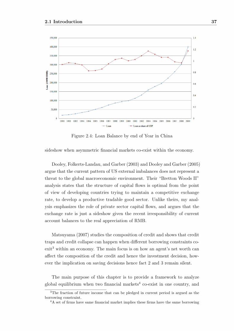
2.1 Introduction 37
Figure 2.4: Loan Balance by end of Year in China
sideshow when asymmetric financial markets co-exist within the economy.
Dooley, Folkerts-Landau, and Garber (2003) and Dooley and Garber (2005)
argue that the current pattern of US external imbalances does not represent a
threat to the global macroeconomic environment. Their “Bretton Woods II”
analysis states that the structure of capital flows is optimal from the point
of view of developing countries trying to maintain a competitive exchange
rate, to develop a productive tradable good sector. Unlike theirs, my anal-
ysis emphasizes the role of private sector capital flows, and argues that the
exchange rate is just a sideshow given the recent irresponsibility of current
account balances to the real appreciation of RMB.
Matsuyama (2007) studies the composition of credit and shows that credit
traps and credit collapse can happen when different borrowing constraints co-
exit3 within an economy. The main focus is on how an agent’s net worth can
affect the composition of the credit and hence the investment decision, how-
ever the implication on saving decisions hence fact 2 and 3 remain silent.
The main purpose of this chapter is to provide a framework to analyze
global equilibrium when two financial markets4 co-exist in one country, and
3The fraction of future income that can be pledged in current period is argued as theborrowing constraint.
4A set of firms have same financial market implies these firms have the same borrowing

2.1 Introduction 38
Figure 2.5: Differences Between SOEs’ and POEs’ Loan Issuance in China
as an important side product to shed some light on facts 1, 2 and 3. The
model is designed to highlight the role of asymmetric borrowing constraints,
in particular the interaction between different borrowing abilities and firms’
entry decisions in shaping the aggregate productivity level, saving and invest-
ment decisions, moreover international trade, global capital flow and world
equilibrium interest rate. The model is fairly standard in its ingredients, and
is based on three building blocks - goods, labour and asset markets, each in-
teracting with the others via equilibrium conditions. I use this model to show
the facts above, can arise naturally when the Chinese financial market hits by
a shock such that after the shock, for one set of the firms (SOEs) it becomes
easier to borrow, while at the same time for the remaining firms (POEs) it
becomes more difficult to borrow.
The dramatic divergence in credit allocation between SOEs and POEs
appears in Figure 2.5, 2.16 and 2.17, where both private and public funding
markets reveal the same striking trend. In the early 1990s, before the cur-
rent account take off in China, rather small differences in borrowing abilities
were observed. Although financial markets have developed across EMs during
the past two decades, the progress has been ‘slightly’ different in China, in
particular SOEs see their borrowing abilities improved much more relative to
POEs’, while the aggregate financing condition improved on average. These
ability.

2.1 Introduction 39
observations rise two important questions, firstly is it plausible to consider an
economy with asymmetric borrowing constraints by a representative economy
with one ‘averaged’ financial market? Secondly, how much does the existence
of asymmetric financial markets ‘contribute’ to not only the Chinese economy
but the world equilibrium? The answer to the first question is “No” and in
this chapter I show many facts in the Chinese economy can be explained by
the co-existence of asymmetric borrowing constraints, furthermore its impact
on shaping the world equilibrium.
Consider a world consists of only two regions - home (China or simi-
lar countries with asymmetric financial markets) and foreign (US and other
economies such as UK), I investigate the implications of a shock in the home
region which worsens the borrowing constraints for one set of firms, at the
same time loosens the borrowing constraints for the remaining firms5. More
importantly, I want to emphasis the equilibrium outcomes in an economy
which has two financial markets, are very different from an economy has just
one financial market which is measured by the average of the two financial
markets. Firms with better access to credit (SOEs) will prevent the POEs
with average productivity enter the market through competition, as a result
only the “super” productive POEs can enter, who produce cheaper output
and drive the large export in the home region (as observed in China see Fig-
ure 2.18). The benchmark framework consists of multiple open economies,
characterized by an overlapping generation structure. This structure pro-
vides scope for both international and intergenerational borrowing. In both
regions, all agents are subject to a borrowing constraint, but the key is that
within the home region, asymmetric borrowing constraints co-exist. The bor-
rowing constraint matters, since prior entering to production, each firm needs6
to borrow against its present discounted value of future profits in order to fi-
nance an initial fixed asset investment7, the fraction of present discounted
value of future profit a firm can pledge is argued as its borrowing constraint8,
and the weighted average across all firms’ borrowing abilities is argued as a
5To be consistent with empirical evidences, throughout this chapter I label firms thathave better access to the credit market as SOEs, and firms that have relatively worseborrowing abilities as POEs.
6I assume the initial fixed cost is too large relative to each agent’s/firm’s saving, so thepotential entrant has to borrow.
7This fixed cost can be seen as the initial set-up cost i.e. firm’s expenditure on purchasingfactory plant or machineries.
8Throughout the chapter, I use words: credit constraint, borrowing constraint andborrowing ability interchangeably, but they all refer to the same concept as defined here.

2.1 Introduction 40
region’s financial market development. Each firm’s profit level is proportional
to its productivity and market share, so for a given level of borrowing ability,
firms’ entry decisions pin down a reservation productivity level where only
firms with higher productivities can enter production. When an ‘asymmetric’
shock hits home agents’ borrowing abilities9, home region’s aggregate demand
for investable assets (or saving) increases because: 1, SOEs take advantage
of better access to the credit market, force the average productive POEs out
of the competition, so only the “super” productive POEs can enter to pro-
duction, therefore in equilibrium the average productivity of POEs is higher
relative to SOEs; 2, the price level of final goods produced using POEs’ inter-
mediate inputs falls (due to cheaper POEs’ input prices), which leads to an
improvement in home region’s trade balance and higher POEs’ profit levels;
3, since POEs can borrow less, POEs owners’ saving increases as they cannot
channel their profits to potential POEs’ investment projects; 4, on the other
hand, SOEs take advantage of better credit market access, boost investment
at the same time generate new investable assets; 5, however, SOEs’ invest-
ment opportunities are limited by their lower (relative to POEs) productivity
levels; 6, therefore the rate of new asset generated by SOEs is not able to
match up with the rate of saving increases in home region; 7, as a result a
large capital outflows towards foreign region; 8, excess saving from the home
region in searching for investable foreign assets, puts downward pressure on
the world equilibrium interest rate.
Finally to close the world asset market equilibrium, the supply of in-
vestable assets increase from the foreign region is driven by a higher demand
for the foreign produced final goods from the households in home region (since
POEs owners receive higher profits, their consumption increases, in turn leads
to a higher demand for both home and foreign produced final goods).
The chapter is organized as follows. Section II will lay out some stylized
facts about the Chinese economy, which rationalize the main assumptions in
this chapter, section III presents some VAR evidence to empirically establish
the connection between the current account and asymmetric borrowing abil-
ities, section IV and V are the core of this chapter where I present the main
model and mechanisms. Section VI supports the main quantitative claims
with different experiments. Section VII concludes with policy implications.
9In particular, this shock increases the borrowing abilities for SOEs and simultaneouslyreduces the borrowing abilities for POEs.

2.2 Some Stylized Facts in the Chinese Economy 41
2.2 Some Stylized Facts in the Chinese Econ-
omy
2.2.1 A Brief History of the Chinese Financial System
and Macroeconomic Trends
China introduced its first economic reform in December 1978. The early re-
forms reduced land collectivization, increased the role of local government
and communities, and experimented with market reforms in a few selected
areas. During which the People’s Bank of China (PBC) departed from the
Ministry of Finance and became a separate entity, at the same time three
state-owned banks took over some its commercial banking business. The
Bank of China (BOC) was given the mandate to specialize in transactions
related to foreign trade and investment; the People’s Construction Bank of
China (CCB), originally formed in 1954, was set up to handle transactions
related to fixed investment (especially in manufacturing sector); the Agri-
culture Bank of China (ABC) was set up in 1979 to deal with all banking
business in rural areas and the PBC was formally established as China’s cen-
tral bank; finally, the fourth state-owned commercial bank, the Industrial
Commercial Bank of China (ICBC) was formed in 1984, and it took over the
rest of commercial transactions of the PBC10. As a result of such reforms in
policy and banking sector, the role of private sector underwent a substantial
change. As rural China was in the ascendancy, where peasants were free to
set up manufacturing, distribution and services businesses that were allowed
to retain profits, pay dividends, issue share capital and even a form of stock
option, state-owned banks rushed to provide the finance (see Huang (2003)).
However, this fundamental shift in policy was not sustained, since the 1990s,
China had adopted the “Shanghai model” of rapid urban development that
favored massive SOEs and big foreign multinational companies, as a result of
which the countryside suffered and indigenous entrepreneurs were starved of
funds and strangled with red tape. As Huang (2003) points out, the worst
weaknesses of China’s state led capitalism - a reliance on creaking state com-
panies rather than more efficient private ones and the weak financial sector
are increasing distorting the economy. This is not the only work that shows
10Note, the four state-controlled commercial banks possess more than 80 percent of thewhole banking sector’s assets and liabilities, and they account for around 80 percent of thelending and 70 percent of the deposit business. Furthermore, given they originally wereassigned different tasks, they do not compete in all business and geographic areas with eachother.

2.2 Some Stylized Facts in the Chinese Economy 42
the non-uniform financial repression; Boyreau-Debray and Wei (2005) docu-
ment that the Chinese banks that are mostly state owned, tend to offer easier
credit to SOEs, so the financial system severely weakens the efficient alloca-
tion of capital, and the private capital does not seem to be large enough to
undo the inefficiency associated with the government dictated finance. As a
result, SOEs finance more than 30 percent of their investment through bank
loans, compared to less than 10 percent for POEs in 2003 (see Song, Storeslet-
ten, and Zilibotti (2011)). Similarly, Dollar and Wei (2007) and James, Jin,
and Gao (2007) report that POEs rely significantly less on bank loans for
investment. Batra, Kaufmann, and Stone (2003) provide survey evidence on
over 10, 000 firms in eighty-one countries around 2000. The subjective per-
ceptions of Chinese entrepreneurs concerning the financial constraints they
face are quite similar to those prevailing in other transitional economies, such
as Croatia, the Czech Republic, Romania, and Slovak Republic, or in poor
economies, such as Ghana and Ethiopia. Furthermore, other forms of mar-
ket financing are marginal for private firms. Despite the rapid growth of the
Chinese stock market in recent years, equity and debt markets continue to
play an insignificant role for POEs, while these markets have become increas-
ing important for large semi-privatized SOEs11 (Neil and Tenev (2001) and
James, Jin, and Gao (2007) chapter 7).
Some surveys organized by the Chinese government reach similar conclu-
sions. A research report based on a private-sector survey conducted in 2002
concludes12:
“In the survey, many private firms say that financing is difficult. The
problem always exists. Government, banks, firms, All-China Federation of
Industry and Commerce have made many efforts but no improvements were
observed. We can see from the survey that lending to the private firms is
scarce and that informal sources represent a substantial part of a firm’s fi-
nance.”
Huang (2003) using firm level data, shows the share of POEs, ranked for-
11In this chapter, I use SOEs and POEs as approximations for the set of firms whohave better and worse borrowing abilities. I notice that some of the semi-privatized SOEs,also fall into the POEs category in my dataset, despite they have ‘good’ access to creditmarket, due to data limitation it is very difficult to disentangle these firms from the otherPOEs, therefore the empirical evidences provide at least a measure of the lower bound ofasymmetric borrowing abilities.
12http://www.china.com.cn/chinese/zhuanti/283076.htm

2.2 Some Stylized Facts in the Chinese Economy 43
mal finance as an important source for starting up has declined from 24.5
percent between 1984 - 1989, to 19.6 percent in 2001.
There are many ways to confirm these results, in this chapter I look at
some direct measurements, namely how much of loan, syndicated loan and
bond have issued by SOEs and POEs (bear in mind that POEs on average
are more profitable compare to SOEs). The total loans outstanding in the
Chinese economy stood at 11.23tr RMB by 2001, and this number had grown
nearly 4 times as large by the end of 2009, to 40tr RMB. Beside the rapid
development in financial market, another striking trend also arose - the differ-
ences between SOEs and POEs in accessing to loan finance13 show in Figure
2.5. Moreover, syndicated loan issuance data in Figure 2.16 confirms the same
message14.
The bond market in China has been dominated by government issuance,
which had an annual growth rate of 27 percent between 1990 and 2005, in
terms of new bond issuance. The second largest component of the bond mar-
ket is called “policy financial bonds”, which are issued by the policy banks and
operated under the supervision of the Ministry of Finance, with the proceeds
of bond issuance being invested in government-run projects and industries.
Despite the fact that corporate bonds are minuscule compared to the size of
government bonds, in terms of the amount of outstanding bonds at the end
of 2005, corporate bonds are only one-eleventh, SOEs also dominated the cor-
porate bond market. A number of possible reasons for the underdevelopment
of bond market in China could be, the lack of sound accounting systems and
high quality bond rating agencies as well as a well-constructed yield curve.
Figure 2.17 shows this striking divergence between corporate bond issuances
between SOEs and POEs.
The credit allocation in China, is far more ‘complicated’ than just the
trend documented above, after the official credit plan was abolished in 1998,
events drive the allocation of the credit on an ad-hoc basis were frequently
implemented ......
13The loan issuance date is obtained from China Monthly Statistics, and the numbersare consistent with Allen, Qian, and Qian (2008)
14The possible reasons behind the trend are out of scope for this chapter, although somepapers have proposed a few possible explanations see Huang (2003) and Shih (2004).
2.2 Some Stylized Facts in the Chinese Economy 44
2.2.2 Some Unexpected Events
Policies designed to control both quality and quantity of new credit issuance,
unintentionally distort the credit allocation in the Chinese economy, in partic-
ular these policy interventions unexpectedly lead to a larger gap in borrowing
abilities between SOEs and POEs. In this subsection I discuss some monetary
policy events, which I argue as unexpected ‘side-effects’, these policy inter-
ventions lead to a distortion in credit allocation within the Chinese economy.
Monetary Policy - 2003 was a major turning point as the Chinese govern-
ment steered away from an expansionary path to prudent monetary policy.
I list a few important interventions carried out by either the People’s Bank
of China (PBC) or the China Banking Regulatory Commission (CBRC) to
control both the quality and the quantity of the new credit issuance, which
describe below.
Credit - Quality
Window Guidance - The PBC started to adopt the policy of “Window
Guidance” in 1998 and it has seemed to be one of the most important tools
to guide the domestic loan increase due to insufficient interest rate elastic-
ity of loans in China. This policy uses benevolent compulsion to persuade
banks and other financial institutions to stick to official guidelines. Despite
the phrase “guidance”, which implies a voluntary aspect in the system, the
PBC has a major influence on lending decisions, especially those of the four
state-controlled commercial banks. In essence, during each of the Window
Guidance meetings, policy makers require banks to improve the quality of
new loan issuance in order to control credit risk. Since it is much more dif-
ficult to accurately assess the credit worthiness of POEs relative to SOEs15,
due to an underdeveloped credit assessment system in China, as a ‘side-effect’,
this policy intervention tends to widen the gap between SOEs’ and POEs’ bor-
rowing abilities.
On June 5, 2003, the PBC initiated a particular Window Guidance pro-
cess to curb the expansionary tendency in the economic cycle 2003/2004. In
the second half of the same year, the PBC asked for Window Guidance meet-
ings three times in the second half of 2003; in those meetings on July 18,
August 11 and September 12, the PBC invited representatives of all Chinese
15One possible reason why lending to SOEs are less risky despite the large non-performingloans, it is majority of the SOEs are backed by local or central government.
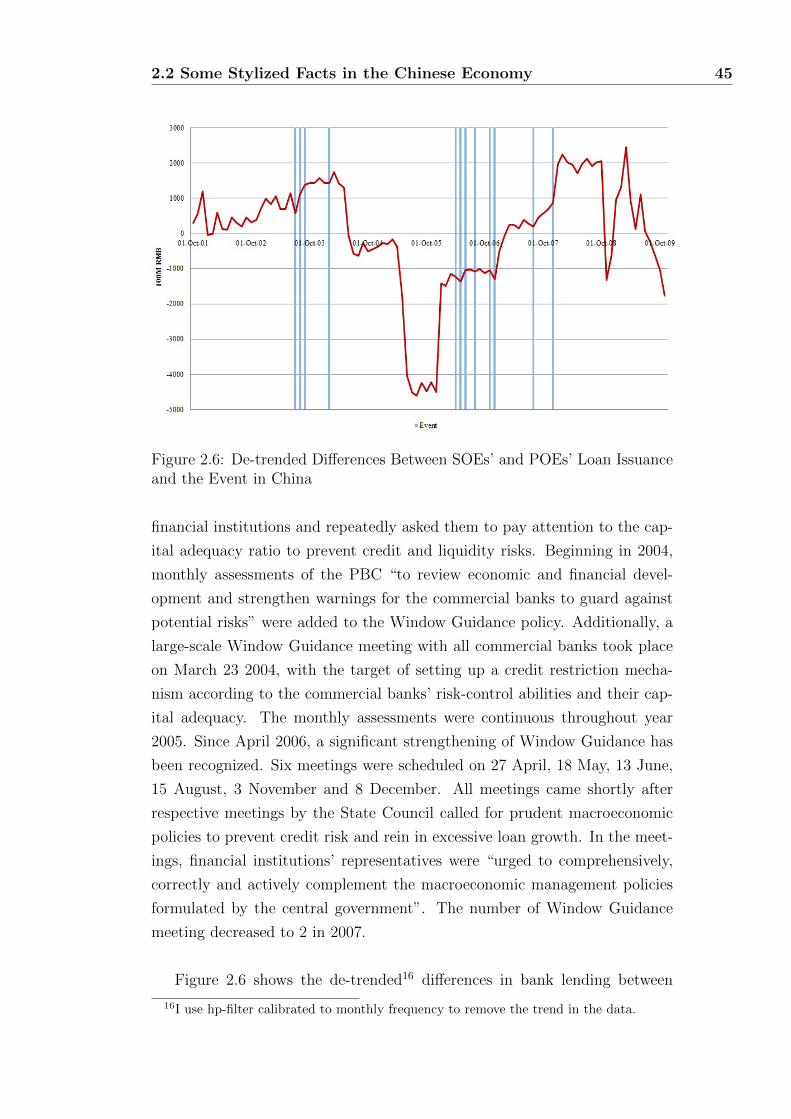
2.2 Some Stylized Facts in the Chinese Economy 45
Figure 2.6: De-trended Differences Between SOEs’ and POEs’ Loan Issuanceand the Event in China
financial institutions and repeatedly asked them to pay attention to the cap-
ital adequacy ratio to prevent credit and liquidity risks. Beginning in 2004,
monthly assessments of the PBC “to review economic and financial devel-
opment and strengthen warnings for the commercial banks to guard against
potential risks” were added to the Window Guidance policy. Additionally, a
large-scale Window Guidance meeting with all commercial banks took place
on March 23 2004, with the target of setting up a credit restriction mecha-
nism according to the commercial banks’ risk-control abilities and their cap-
ital adequacy. The monthly assessments were continuous throughout year
2005. Since April 2006, a significant strengthening of Window Guidance has
been recognized. Six meetings were scheduled on 27 April, 18 May, 13 June,
15 August, 3 November and 8 December. All meetings came shortly after
respective meetings by the State Council called for prudent macroeconomic
policies to prevent credit risk and rein in excessive loan growth. In the meet-
ings, financial institutions’ representatives were “urged to comprehensively,
correctly and actively complement the macroeconomic management policies
formulated by the central government”. The number of Window Guidance
meeting decreased to 2 in 2007.
Figure 2.6 shows the de-trended16 differences in bank lending between
16I use hp-filter calibrated to monthly frequency to remove the trend in the data.

2.2 Some Stylized Facts in the Chinese Economy 46
SOEs and POEs, and the month which Window Guidance meeting (“event”)
was carried out. Data suggests that following the event of Window Guidance,
an unexpected increase between the loans held by SOEs and POEs is ob-
served, which confirms lack of a robust credit worthiness assessment system
in China, as a result of such, any policy designed to control the quality of new
credit issuance unintentionally widen the borrowing abilities between SOEs
and POEs.
Remark: I notice the Window Guidance is not the only event which causes
the difference between POEs’ and SOEs’ borrowing abilities, as it is always
difficult to identify these events, but Figure 2.6 does suggest Window Guid-
ance is one of these events which unexpectedly widen the borrowing abilities
between SOEs and POEs17.
Credit - Quantity
Despite the fact that credit plan was officially abolished in 1998, preferen-
tial lending to certain areas and industries is still observed. During the recent
economic crisis, the Chinese government implemented a 4 trillion RMB stim-
ulus package to prevent a slowdown in the Chinese economy from the global
financial crisis. The package was injected into economy via central government
direct credit and instructed bank lending, however many evidences suggest
the majority of the funding was channeled to SOEs. Thus, credit alloca-
tion does not follow cost-utility criteria, in the sense that credit allocation
is not steered by the price but by the required or desired amount of money.
In essence, there is still a quasi credit plan in effect, although, most impor-
tantly, compared to the long-term determination of the official credit plans
of former times, the amount of driven credit allocation of today serves on an
ad-hoc basis. Notice, since the four state-controlled commercial banks are in
favor of lending to SOEs; therefore, any form of credit tightening at aggre-
gate level will pass through to POEs relatively more than SOEs. As a result,
any policies designed to control the quantity of new credit issuance, will also
unintentionally lead to a larger gap in borrowing abilities between SOEs and
POEs.
Reserve Requirement - Table 2.1 shows the development of the reserve
requirement in China since 1985. This table illustrates how the regulators
17Year 2005 stood out from the trend, one reason behind the huge fall was due to a dryup in new loan issuance at national level, as the planned target loan growth was expectedat 14.1 percent and the actual growth was at 9.8 percent.

2.3 Evidence from a Simple VAR 47
passively used the instrument between 1985 and 1998 and the ever increas-
ing activity since 2003. These moves partly reflect how PBC’s regard reserve
requirement ratio as a main instrument to control liquidity in the financial
system, and also show how the PBC have restrained the monetary and credit
aggregates of the economy since 2003, and more severely in the recent years.
Open Market Operations18(OMO) - On May 26th, 1998 the Chinese au-
thorities officially re-introduced open market operations. Before 27 February
2003, open market operations were generally carried out every Tuesday. Since
11 May 2004, the operation has generally been conducted on a two day a week
basis. Open market operations include national bonds, central bank bills and
financial bonds from other financial institutions(the so called policy bank).
From May 1998 to mid-2000 only repurchasing operations were utilized for
the sole purpose of issuing base money. Since mid-2000, however, a major
shift has taken place: repurchase agreements were increasingly used to with-
draw base money from the financial system. In 2003, the PBC started to
additionally issue central bank bills19.
2.3 Evidence from a Simple VAR
Figure 2.7 and 2.8, present impulse responses (with 68 and 95 percent con-
fidence bands respectively) from a simple VAR with the Chinese current
account balance(CA) and the differences between loan issued to SOEs and
POEs(Ldiff), between 1994 and 2009. I use this VAR20 to document the key
relationships in the data, and to provide a qualitative assessment of the sim-
ulated model.
Here all the variables are expressed in logarithmic terms. The shocks are
othogonalized in the order of the differences between log of loans issued to
SOEs and POEs and the log of Chinese current account balance. Due to data
limitation, the analysis can only be carried out at annual frequency; however,
the results already suggest a positive response to the current account balance
18see Table 2.2 for a list of the OMOs19see Table 2.3 for a list of the central bank bills, designed to withdraw the liquidity in
the system.20These graphs are constructed following generalized impulse response function method
in Pesaran and Shin (1998), therefore, I do not need to make any assumption on the orderingvariables. However, similar result is obtained if instead using Cholesky decompositionassuming that the policy makers do not foresee the current period current account balancewhen they carry out policy interventions.

2.3 Evidence from a Simple VAR 48
Figure 2.7: IRF 1 - Response of the Chinese current account balances to onestandard deviation of loan issuance shock
Figure 2.8: IRF 1 - Response of the differences between SOEs’ and POEs’loan issuance to one standard deviation of loan issuance shock

2.4 The Basic Set Up - A Closed Economy 49
after a shock to the borrowing ability, and it converges back to 0 after 2 time
periods.
Furthermore, I carry out a similar exercise but with improved sample
size. Figure 2.19, 2.20 and 2.21 present impulse responses from a VAR with
the log of US vs China bi-lateral current account balances(CA), the log of
Chinese GDP(GDP), and the differences between loans issued by SOEs and
POEs(Ldiff), at quarterly frequency. The results confirm a positive response
of both the current account balance and China’s GDP after a shock to the
borrowing ability.
In this chapter, I construct and estimate a model that is consistent with
these facts and that can be used for policy analysis. I start with a basic
model, which conveys the intuition.
2.4 The Basic Set Up - A Closed Economy
Time is continuous, infinitesimal agents are born at a rate ρ per unit time and
exist at the same rate, population mass remaining constant. A cohort born
at time zero has a size, as of time t, of ρe−ρt, and the size of the population
at any time t is∫ t−∞ ρe
−ρ(t−s)ds = 1.
Following Blanchard (1985), I assume that private markets provide insur-
ance, and agents will contract to have all of their wealth return to the life
insurance company contingent on their death, such that agents do not need
to worry about longevity risk of death; more specifically, if an agent’s wealth
is w, they will receive ρw if they do not die, and pay w if they die.
Consumption
• Individual Consumption.
Denote c(s, t), a(s, t) and w(s, t) consumption, per period income and
wealth of an agent born at time s, as of time t. Let rt be the interest rate at
time t, τ be the agent’s time discount. Under the assumption that instanta-
neous utility is logarithmic, agent maximizes:∫ ∞t
logc(s, v)e(τ+ρ)(t−v)dv (2.1)

2.4 The Basic Set Up - A Closed Economy 50
subject to the dynamic budget constraint:
dw(s, t)
dt= (rt + ρ)w(s, t) + a(s, t)− c(s, t) (2.2)
which can be integrated to give:∫ ∞t
c(s, v)e−∫ vt (r(µ)+ρ)dµdv = w(s, t) + h(s, t) (2.3)
So the optimal consumption path is:
c(s, t) = (ρ+ τ)(w(s, t) + h(s, t)) (2.4)
Individual consumption depends on total individual wealth, with propen-
sity (ρ+ τ).
where:
h(s, t) =
∫ ∞t
a(s, v)e−∫ vt (r(µ)+ρ)dµdv (2.5)
• Aggregate Consumption.
Let Ct, Wt and Ht denote aggregate consumption, wealth and income at
time t.
Aggregating equation 2.4 across all agents in the economy at time t leads
to:
Ct =
∫ t
−∞c(s, t)ρeρ(s−t)ds = (ρ+ τ)(Wt +Ht) (2.6)
Now, I assume that household income is equally distributed: a(s, v) = av
for all s, i.e. a household’s income is independent of when he was born, fur-
thermore define Av =∫ v−∞ a(s, v)ρe(s−v)ρds.
The aggregate income can be expressed as:
Ht =
∫ t
−∞h(s, t)ρeρ(s−t)ds
=
∫ ∞t
Ave−∫ µt (rµ+ρ)dµdv (2.7)
Differentiate with respect to time:
dHt
dt= (rt + ρ)Ht − At (2.8)

2.4 The Basic Set Up - A Closed Economy 51
The aggregate wealth:
Wt =
∫ t
−∞w(s, t)ρeρ(s−t)ds (2.9)
Differentiating with respect to time gives:
dWt
dt= w(t, t)− ρWt +
∫ t
−∞
dw(s, t)
dtρeρ(s−t)ds
= w(t, t)− ρWt + (rt + ρ)Wt + At − Ct (2.10)
to arrive at the second line, I used equation 2.4.
Furthermore, I assume that agents have no initial wealth w(t, t) = 0, then
aggregate wealth is characterized by:
dWt
dt= rtWt + At − Ct (2.11)
Collecting equations:
Ct = (rt + τ)(Wt +Ht)
Ht = (rt + ρ)Ht − AtWt = rtWt + At − Ct (2.12)
These equations reduce to:
Ct = (rt − τ)Ct − ρ(ρ+ τ)Wt
Wt = rtWt + At − Ct (2.13)
Production
Two types of good exist, final good B is used for consumption and inter-
mediate goods are used for final good production.
• Final Good Production.
Final good B is produced by aggregating ωB differentiated intermediate
inputs.
YB,t =(∫ ωB,t
0
yB,t(i)θ−1θ di
) θθ−1
(2.14)

2.4 The Basic Set Up - A Closed Economy 52
Final good B producer faces perfect competition, who minimizes its total
cost by choosing the level of intermediate inputs, for a given level of output
YB,t, yields the following demand for intermediate input yB,t(i) at time t:
y∗B,t(i) =1
ωB,t
(pB,t(i)PB,t
)−θYB,t (2.15)
Where, PB,t is the price index for final good B at time t and pB,t(i) is the
price for intermediate inputs i.
The price for good B has the following expression (more on this later):
PB,t = ω1/θB,t
(∫ ωB,t
0
(pB,t(i))1−θdi
) 11−θ
(2.16)
• Intermediate Good Production.
Each intermediate good producer faces monopolist competition, who takes
the demand as given (from the final good producer), and sets a price with
a constant markup over its marginal cost. Intermediate good production
requires only one factor of input - labour, which is inelastically supplied at
aggregate level. Firm’s technology is represented by a cost function that
exhibits constant marginal cost. Labour is thus a linear function of output
y: l = yϕ
. All firms have different productivity levels indexed by ϕ ≥ ϕmin.
Higher productivity is modelled as producing a symmetric variety at lower
marginal cost, or it can also be thought as producing a higher quality variety
at equal cost. Regardless of its productivity, each firm faces a residual demand
curve with constant elasticity θ and thus chooses the same profit maximizing
markup. This yields a pricing rule for a firm producing variety i:
pB,t(i) =( θ
θ − 1
)( vtϕ(i)
)(2.17)
Where the profit function for an intermediate firm i at time t can be
written as:
πB,t(i) =(pB,t(i)−
vtϕ(i)
)yB,t(i)
=(( v1−θ
t
θ − 1
( θ
θ − 1
)−θ)ϕθ−1(i)
ωB,tP θB,tYB,t (2.18)
vt is the wage rate at time t, which is determined by the labour market

2.4 The Basic Set Up - A Closed Economy 53
clearing condition, to arrive the second line, I substitute in the demand curve
for intermediate good i.
Intermediate Firm Entry and Exit Decisions
• Entry.
There is a large (unbounded) pool of prospective entrants into interme-
diate goods production. I assume that firms are owned by agents21, initially
each firm draws a specific initial productivity parameter ϕ from a common
distribution g(ϕ). g(ϕ) has positive support over [ϕmin,∞) with correspond-
ing cumulative distribution G(ϕ). To enter, each firm must makes an initial
investment modelled as a fixed entry cost FB > 0, which is thereafter sunk. To
finance this initial fixed cost firm needs to borrow, the fraction of its present
discounted value of future profits, the firm can pledge (denote by δt) reflects
this firm’s borrowing ability. Therefore each firm given its productivity draws,
knowing the entry cost (FB) and its borrowing ability, they simultaneously
choose to enter the intermediate goods production or not.
Therefore, a potential entrance will enter intermediate good production
if and only if he makes a non-negative profit by entering22 and has sufficient
borrowing to finance the initial fixed investment that is:
δπ∞(i)− FB ≥ 0 (2.19)
Where π∞(i) denotes the present discounted value of future profits for
intermediate firm i23.
π∞(i) =
∫ ∞t
πs(i)e−∫ st (r(τ)+ρ)dτds (2.20)
Let Πt denotes the aggregate (across all intermediate firms) profit in the
economy at time t.
Πt =
∫ ωB,t
0
πt(i)di (2.21)
The reservation productivity (ϕ∗B,t) at time t is determined at which the
firm is indifferent between enter or not, therefore, all the potential entrants
21This assumption serves one purpose: intermediate firms’ profits will transfer to house-hold.
22This condition requires π∞(i)−FB ≥ 0, since δ < 1 this condition always hold as longas firm’s borrowing condition is satisfied.
23Note, since the agent owns the firms, firms also exit at the point agent dies.

2.4 The Basic Set Up - A Closed Economy 54
with a productivity draw higher than ϕ∗B,t, will decide to enter the production
in intermediate good.
δtπ∞(ϕ∗B,t)− FB = 0 (2.22)
Given the reservation productivity, the equilibrium number of intermedi-
ate good firms (ωB,t) at time t is pinned down by:
ωB,t = 1−G(ϕ∗B) (2.23)
Remark 1: Under this setting, as δt → ∞, that is FB → 0, the reserva-
tion productivity approaches to the lower bound of productivity distribution
(ϕ∗B,t → ϕmin), where ϕmin can be seem as the TFP level in the region.
Remark 2: The fixed entry cost (FB) is treated as constant across different
firms despite their output and profit levels, seems at first instant implausible.
However, letting the fixed entry cost vary with firm’s profit level is equiv-
alent to the situation with varying borrowing abilities and a constant fixed
entry cost (F f ). For example: let F v(Π∞) denote the fixed cost, a firm has
to pay prior to entry, which is a function of the profit level, for simplicity, I
assume F v(Π∞) = F f ∗ (Π∞)β, where F f is a constant and 0 < β < 1, then
firm’s entry decision becomes δtπ∞(i) − F v(Π∞) = 0 which is equivalent as
δ1
1−βt π∞(i)− (F f )
11−β = 0.
• Exit.
Once a firm successfully entered the intermediate good production, it has
to pay a running cost ft (to its current owner/agent) each period, which is
financed by firm’s current period profit24. For example, this cost can be seem
as the additional compensation to the managers. Therefore, intermediate firm
can only continues to produce if and only if:
πt(i)− ft ≥ 0 (2.24)
Otherwise, firm exists the production at time t. I discuss ft in more detail in
the calibration section.
24Similar results are concluded if I assume instead firm finance this cost by using retainedearnings.

2.4 The Basic Set Up - A Closed Economy 55
Asset Market
The corporate bond issued by intermediate firms (to finance the initial
fixed cost) is the only saving option (investable assets) for the agents, which
yield a return of δtΠt per unit time.
Let Vt denotes the total corporate bond outstanding at time t. By arbi-
trage, the instantaneous return from holding a unit of bond rt, satisfies:
rtVt = δtΠt + Vt (2.25)
The equation says, return on bond equals the divined price ratio δtΠt/Vt plus
the capital gain Vt/Vt.
Recall the total savings accumulated by active agents at date t, denote
by Wt is increasing with the income and the return accumulated on savings,
decreases with consumption.
Wt = rtWt + At − Ct (2.26)
Asset market equilibrium imposes Vt = Wt, which pins down the domestic
equilibrium interest rate.
Labour Market
For simplicity I assume that labour are inelastically supplied at aggregate
level L, therefore the labour market clearing condition imposes:∫ ωB,t
0
l(i)di = L (2.27)
where, l(i) is the employment level in intermediate firm (i) and L is the
population size, moreover, the wage rate is pinned down by:∫ ωB,t
0
l(i)di =
∫ ωB,t
0
yB,t(i)
ϕt(i)di (2.28)
gives the equilibrium wage rate:
vt =(θ − 1
θ
)(
α
α + 1− θ)
1θϕ
θ−1θ PB,tY
1θB,t (2.29)
2.5 The World Economy 56
Given the wage rate, the aggregate household income at time t is the
sum of the wage incomes, profits from intermediate firms minus the fixed
investments.
At = vtL+ (1− δt)Πt − ρwtFB (2.30)
Note, the intermediate firm owners can only keep (1 − δt) fraction of the
profit each period and remaining δt fraction of the profits are paid back to
the bond holders.
2.5 The World Economy
This section services two purposes: firstly, as the title suggests, to consider
an open economy version of the model above, which provides the framework
to study global equilibrium; Secondly, to introduce the asymmetric financial
markets.
The world is sliced up to two large regions, home (h) and foreign (f) i.e.
j = (h, f), home can be seen as region consists of developing countries i.e.
China, and foreign region consists of advanced economies i.e. U.S. or U.K. as
discussed before.
Each of the regions is described by the same setup up as in the closed econ-
omy, let Cjt denotes the consumption of country j at time t. Furthermore,
final goods and corporate bonds are traded across the border, and intermedi-
ate goods and labour are only used within each region for production.
Recall the consumer’s inter-temporal consumption decision
Cjt = (rt − τ)Cj
t − ρ(ρ+ τ)W jt (2.31)
Each region j produces one type of final goods i.e. Bh,Bf , which are
traded across the border, therefore, consumer in each region consumes both
final goods, with intra-temporal consumption decision given by:
Cjt = (1/2(cjBh,t)
θ−1θ + 1/2(cjBf,t)
θ−1θ )
θθ−1 (2.32)
Given CES preference, demand for good Bj by the residents in region
z = h, f satisfy:
czBj,t =(PBj,tP zt
)−θCzt (2.33)
2.5 The World Economy 57
The aggregate demand for final good Bj is the sum of demand from both
regions, hence equilibrium in final good markets require:
YBj,t = chBj,t + cfBj,t (2.34)
with the following price index P jt and j = h, f :
P jt = (1/2P 1−θ
Bh,t + 1/2P 1−θBf,t)
11−θ (2.35)
P jt denotes region j’s price index for consumption bundle Cj
t , which is
normalized to 1. PBj,t denotes the price index for the goods produced in
country j at time t.
PBj,t = ω1/θBj,t
(∫ ωBj,t
0
(pBj,t(i))1−θdi
) 11−θ
(2.36)
Therefore, profit for an intermediate firm i in country j can be written as:
πBj,t(ωBj, ϕ(i), i) =(pBj,t(i)−
vj,tϕ(i)
)yBj,t(i)
=( v1−θ
t
θ − 1
( θ
θ − 1
)−θ)ϕBj,t(i)θ−1
ωBj,t(Ch
t + Cft ) (2.37)
Asymmetric Financial Markets
I assume that in region f all potential entrants can borrow the same frac-
tion δf of their present discount value of future profits to finance the initial
set up cost, hence there is no asymmetric financial market in region f , or
put it simply all potential entrances in foreign region has the same borrowing
ability. However, in the home region, I assume q share of the total potential
entrants (SOEs) can borrow δSOEs fraction and the remaining (1 − q) share
of firms (POEs) can borrow δPOEs fraction of their present discount value of
future profits. Moreover, the aggregate financial condition at home region is
defined as δht = q ∗ δSOEst + (1− q) ∗ δPOEst .
The entry decision rule within each region is the same as in the closed
economy, where the potential entrant will only decide to enter if he can make
non-negative profit conditional on having sufficient funds to finance the initial
fixed investment:

2.5 The World Economy 58
In the foreign region, an agent will enter production if:
δfπf∞(i) ≥ FBf (2.38)
The reservation rule is when agent is indifferent between entry or not to
enter, leads to the reservation productivity (ϕf∗t ) at time t:
ϕf∗t =(
(δfκ
FBf)
∫ ∞t
(vfs )1−θω−1Bf,s(C
hs + Cf
s )e−∫ st (rµ+ρ)dµds
) 11−θ
(2.39)
where κ = ( 1θ−1
)1−θ is a constant, differentiate with respect to time:
ϕft = (δft κ(vft )1−θ
FBf ∗ (θ − 1)) ∗ ω−1
Bf,t ∗ (ϕft )θ(Ch
t + Cft )− rt + ρ
(θ − 1)ϕft (2.40)
The equilibrium number of intermediate firms at time t is pinned down
by:
ωBf,t = 1−G(ϕf∗t ) (2.41)
In the home region it is more interesting, SOEs’ entry decisions are char-
acterized by:
δSOEsπh∞(i) ≥ FBh (2.42)
Gives:
ϕh∗δSOEs,t = (δSOEsκ(vht )1−θ
FBh ∗ (θ − 1)) ∗ ω−1
Bh,t ∗ (ϕhδSOEs,t)θ(Ch
t + Cft )− rt + ρ
(θ − 1)ϕhδSOEs,t
(2.43)
For the remaining (1− q) POEs the enter decision:
δPOEs ∗ πh∞(i) ≥ FBh (2.44)
Gives:
ϕh∗δPOEs,t = (δPOEsκ(vht )1−θ
FBh ∗ (θ − 1)) ∗ ω−1
Bh,t ∗ (ϕhδPOEs,t)θ(Ch
t + Cft )− rt + ρ
(θ − 1)ϕhδPOEs,t
(2.45)
Hence the equilibrium number of firms in home economy is:
ωBh,t = 1− q ∗G(ϕh∗δSOEs,t)− (1− q) ∗G(ϕh∗δPOEs,t) (2.46)
2.6 Quantitative Analysis 59
World Asset Market
Similar to the closed economy, each region j’s wealth evolves according to:
W jt = rtW
jt + Ajt − C
jt (2.47)
rtVjt = δtΠ
jt + V j
t (2.48)
Let, Wwt denote the world demand for asset or world’s total saving; simi-
larly V wt denotes the total asset outstanding in the world:
Wwt = W h
t +W ft (2.49)
V wt = V h
t + V ft (2.50)
The world equilibrium interest rate at time t, is pinned down by the global
asset market clearance condition:
V wt = Ww
t (2.51)
Finally, I define the current account balance and trade balance:
CAjt = W jt − V
jt
TBjt = PBj,tY
zBj,t − PBz,tY
jBz,t (2.52)
where j, z = h, f ; j 6= z.
2.6 Quantitative Analysis
In this section, I investigate whether facts observed both at national and in-
ternational level: 1, the productivity differential between SOEs and POEs in
China; 2, the sustained Chinese current account surplus; and 3, the stubborn
decline in long run real interest rate, are results of the co-existence of two dif-
ferent borrowing constraints within the home region. I start the investigation
by looking at when a negative shock hits the aggregate financial market in
the home region (a fall in both δSOEst and δPOEst hence δht ), i.e. a temporary
crash in the Chinese financial market or a contraction in monetary policy. I
will then layout the core results in the following subsection, where I show how
the facts are generated, when the Chinese economy hits by a more ‘realistic’
asymmetric financial shock such that, SOEs see their credit constraints re-
laxed at the cost of tightening borrowing constraints for the remaining POEs.

2.6 Quantitative Analysis 60
Given it is widely accepted that, the aggregate financial condition in China
has developed in the past, I show all the results hold still true, even in the
case where aggregate credit condition in China is improving, as long as the
differences between SOEs’ and POEs’ borrowing abilities exist. That is δh
grows but δSOEs > δPOEs i.e. an implementation of expansionary monetary
policy to inject more credit in the economy, plus its unintended consequences
which lead to a wider gap in borrowing abilities between SOEs and POEs.
2.6.1 A Calibration
I begin by discussing the parameter calibration in the home region. Pref-
erence parameters are standard, for simplicity I assume the intertemporal
elasticity of substitution is same for the final good producer and household’s
final good consumption, and it is fixed at θ = 2.1. The time discount factor
for the household is set at τ = 0.02 to match the average real interest rate in
China between 2002 and 201025. The productivity ϕ follows Pareto distribu-
tion, with shape parameter α equals to 2.6 and the minimum productivity set
to equal 0.2, these assumptions follow Corcos, Gatto, Mion, and Ottaviano
(2009), where they show that Pareto distribution closely fits the observed
firm productivity distribution, and using a large firm level dataset from E.U.,
they estimate share parameter α across different manufacturing industries.
The exogenous entry and exit rate is calibrated to 5.5 percent, which was
calculated as the (yearly) average of the firm’s entry and exit rate in China
between 2002 to 2006 from Brandt, Biesebroeck, and Zhang (2009)26. The
initial fixed cost (FB) is set to equal to 0.32 which is calibrated to the ratio
between total fixed investment and total output across Chinese manufactur-
ing industries. The share of SOEs - q, I calibrated to 0.5 to match the average
SOEs’ output share in 26 manufacturing industries between 2002 and 2007.
To make the model more manageable, I assume ft(i) = πt(i)π∞(i)
FBδ
, by making
this simplification assumption the number of state variables which I need to
keep track of, is significantly reduced. Finally, since it is difficult to measure
borrowing constraints directly, I calibrate the value of δh indirectly (follow-
ing Caballero, Farhi, and Gourinchas (2006)), to do so I assume the steady
state interest rate to be around 3 percentage points, which implies a value of
25Data from World Development Indicator.26Figure 1 in Brandt, Biesebroeck, and Zhang (2009) suggests between 2003 and 2006,
there are on average 2.75 percent new SOEs, 13.75 percent new POEs enter into and 2.9percent of SOEs, 5.6 percent of POEs exit from current production. One caveat, some ofthe new semi-privatized SOEs entrance, enters the production as POEs in the data, thiscould explain the low SOEs entering rate.

2.6 Quantitative Analysis 61
δh = 0.12.
Given the initial calibrations at home, I now explore a number of different
cases which will lay out the parameter calibrations in the foreign economy.
2.6.2 A Temporary Borrowing Ability Shock
I start with the analysis of a temporary collapse in δh. In order to reveal
the impacts and mechanisms of this shock, I make the assumption that both
home and foreign regions start at same line or operate at the same steady
state prior the shock.
Assumption 1 (Initial Conditions): The world is initially symmetric, more
specifically δh = δPOEs = δSOEs = δf . Moreover, FBh = FBf .
Since both regions are initially symmetric, there is no initial net trade and
capital flow. Suppose now, unexpectedly at t = 0, δh drops temporarily to
δSOEs = δPOEs = δh < δf . The fall in δh in general could result from, a crash
in a bubble, a monetary tightening (as I argued before) or a significant loss
of informed and intermediation capital.
Note that the definition for current account in this chapter excludes, as
does the one of national accounts, unexpected valuation effects - unexpected
capital gains and losses from international positions. It is not a relevant issue
for now, since the only surprise takes place at date 0, when agents are not
holding international assets.
Also note that, since CAht + CAft = 0, I need only describe one of the
current accounts to characterize both. Henceforth, I will focus on describing
the behaviour of CAht , with the understanding that this concept describes
features of the global equilibrium rather than h-specific features.
Figure27 2.22 characterizes the path for some key variables following a
collapse of δh calibrated so that h’s investment level drops by just above 25
percent relative to the steady state value. Panel A (CA) shows that h’s cur-
rent account exhibits an initial surplus of 1.6 percent of GDP. This sharp
and concentrated initial spike may be partly due to the lack of smoothing
27Note: each of the graphs plots the response of a variable as a percentage deviationfrom its steady state value after the shock, unless otherwise stated.

2.6 Quantitative Analysis 62
mechanism in the model. Still, note that in this fast environment, current
account surplus does not disappear after 2 time periods. The main driver
behind these results, is the gap between home saving and home asset issuance
rates. The interest rate drops by more than 5 percent before rising back to
its original steady state value of 2.9 percentage points.
In summary, the model is able to generate, simultaneously, a large current
account surplus and a decline in real interest rate which are consistent with
Caballero, Farhi, and Gourinchas (2006).
2.6.3 An Asymmetric Borrowing Abilities Shock and
Trend I
Given that the aggregate credit condition has improved in EMs, especially in
China, it is difficult to reconcile any facts as the consequences of a collapse in
financial market. Therefore, in this subsection, I consider a temporary credit
shock in the home region, such that one set of firms (POEs) became harder
to borrow, and the remaining firms (SOEs) became easier to borrow at the
same magnitude, most importantly the aggregate credit condition remains
unchanged after the shock, that is, δSOEs increases, δPOEs decreases but δh
remain unchanged28. As mentioned in earlier section, the empirical evidences
revealed an important trend in the Chinese economy. Namely, SOEs consis-
tently had better access to credit market relative to POEs. Therefore, I con-
sider two cases, firstly I assume prior to the shock, both SOEs and POEs have
the same borrowing abilities (δSOEs = δPOEs), hence all the results are driven
by the asymmetric borrowing ability shock moreover firm’s endogenous entry
decision, it is important as these decisions collectively affect the aggregate
profit levels in the economy; secondly, I incorporate the trend δSOEs > δPOEs
into the main mechanism, in particular I assume SOEs on average can bor-
row 40 percent (a number calculated from annual Chinese loan issuance data)
more relative to POEs.
One caveat, standard models imply that capital flows from low to high
growth economies; I argue here that this conclusion does not carry over to
the case where productive agents have limited ability to generate assets in or-
der to carry out investment. In particular, high productivity combined with
28I define an asymmetric borrowing abilities shock is a shock, such that after the shockPOEs became harder to borrow and SOEs became easier to borrow, however I make noassumption on the aggregate borrowing condition, as you shall see the reason later.

2.6 Quantitative Analysis 63
low ability to generate asset in the home region imply greater savings which
in turn lower long-run interest rates and generate large capital outflow.
Assumption 2 (Initial Conditions): The world is initially symmetric, with
δh = δf . Moreover, prior to the shock, SOEs and POEs have the same bor-
rowing abilities δSOEs = δPOEs and FBh = FBf .
Figure29 2.9 2.10 and 2.11 illustrate the entire path following the asymmet-
ric borrowing ability shock in the home economy. I explore the transmission
paths in detail:
Immediately after the shock, SOEs’ borrowing ability rises at the cost of
fallen POEs’ borrowing ability, where the aggregate credit condition remains
unchanged in the home region (see Panel 1, 2 and 3). The reservation pro-
ductivity for POEs to enter production becomes higher (see Panel 5), whereas
the reservation productivity for SOEs (Panel 4) falls due to better access to
credit market. Furthermore, since a firm’s profit level is positively correlated
with its market share, SOEs deter the marginal POEs enter into production
(competition effect); this creates a second order effect30 which limits only the
‘super’ productive POEs can enter and survive in the intermediate good pro-
duction. Most importantly, this competition effect leads to a higher increase
in averaged POEs’ productivities than the fall in averaged SOEs’ productivi-
ties, hence the net aggregate productivity at home region increases (see Panel
6).
The equilibrium number of POEs falls and SOEs rises, as shown in Panel
7 and 8, and aggregate number of intermediate good producers increase, due
to a large number of SOEs enter by taking advantages of the better access to
credit market (see Panel 9).
The intermediate good price level is inversely related to its producer’s
productivity level, hence the average price of POEs produced intermediate
outputs fall, and vice versa for the intermediate output produced by SOEs.
The final good producer sets the final good price at its marginal cost, since
29Note: each of the graphs plots the response of a variable as a percentage deviationfrom its steady state value after the shock, unless otherwise stated.
30Although the effect is second order, as this chapter shows its impact on shaping globalequilibrium is large in magnitude, therefore it is important to understand the mechanismsbehind this effect.

2.6 Quantitative Analysis 64
the aggregate cost of intermediate input falls due to more productive POEs
(the competition effect, see Panel 10 and 11) the price of home produced final
goods fall (see Panel 12). This leads to an improvement of the trade balance
in the home region31 (see Panel 15).
Furthermore, an intermediate firm’s profit level is positively related to its
productivity level, as shown in Panel 13 and 14, POEs see their profits rise
and a fall in SOEs’ profit level.
Higher profit level translates to a higher consumption level and saving rate
for the households who own POEs (see Panel 17 and 20), and the opposite
story is true for SOEs owners (see Panel 16 and 19). The key message here
is that the rise in averaged POEs’ productivities is higher than the fall in
averaged SOEs’ productivities due to competition effect at the enter to pro-
duction stage. Therefore the aggregate consumption level and saving rate rise
in home region (see Panel 18 and 21).
In the home region, POEs owners drive the high saving rate due to larger
profit levels, and SOEs become the drivers behind the high investment rate
due to better access to credit, as confirmed in Panel 20 and 22. Hence, SOEs
are the main drivers behind the new asset issuance in the home region.
However, the average productivity level of SOEs is lower relative to POEs’
average, since saving rate is driven by POEs (see Panel 20), and the new asset
issuance rate is driven by SOEs (see Panel 22). The aggregate saving rate
increases (see Panel 21), and the aggregate new asset issuance falls (see Panel
25). As a result, capital flows from home to foreign region, as Panel 26 shows.
The final good produced in the home region is a close substitute for the
foreign produced final good, foreign final good output level is downsized as
shown in Panel 27 (households substitute their consumption in foreign pro-
duced final goods with the cheaper final output produced by the home region).
This environment leads to a fall in aggregate profit level and saving rate in
foreign region (see Panel 28 and 29). However, the foreign households’ con-
sumption levels do not fall as much, since they are taking advantages of the
cheaper import from the home region (see Panel 30).
31In Figure 2.18 suggests that Chinese export is mainly driven by the POEs.
2.6 Quantitative Analysis 65
Furthermore, the higher consumption levels in the home region (together
with lower world interest rate) increases the demand for foreign produced final
goods. This increase in demand for foreign produced final goods, translates
into a higher number of intermediate good producers, as a result the new
asset issuance increases in the foreign region (see Panel 31).
The saving accumulated by POEs owners in searching for investable as-
sets, drives up the world saving rate at the same time new investable asset
from the foreign region leads to an increase in world asset supply. These
observations have two consequences: 1, a large capital outflow from home to
foreign region; 2, the world equilibrium interest rate falls (see Panel 26 and
34). This fall in interest rate feeds back to encourage more investment and
consumption in both regions. Therefore the final good output in home region
rises, this increase is partly driven by the external demand from foreign region
(see Panel 35). Furthermore, the rise in home produced final output is also
driven by an internal factor - the re-allocation of labour towards the more
productive POEs within the home region, since there are no job searching
nor matching frictions, labour can easily switch between jobs. Finally, wage
rate in home region rises (see Panel 36).
Overall, this asymmetric borrowing ability shock is able to generate: 1, a
productivity differential between SOEs and POEs; 2, a large current account
surplus in home region; and 3, a fall in world equilibrium interest rate.
In Figure32 2.23 2.24 and 2.25, the green lines represent the path with
the initial conditions where SOEs have better borrowing ability than POEs
i.e. δSOEs > δPOEs, in particular I assume SOEs can on average borrow 40
percent more relative to POEs. The blue lines represent the base line results
as shown above, where initially SOEs and POEs have the same borrowing
abilities. These results suggest that by incorporating the trend into the main
mechanism, all the impacts point to the same direction, and the trend ampli-
fies the propagation mechanism, lead to larger impact on all variables.
32Note: each of the graphs plots the response of a variable relative to its steady statevalue after the shock, unless otherwise stated.

2.6 Quantitative Analysis 66
Figure 2.9: Equilibrium Path after an Asymmetric Borrowing Shock - 1

2.6 Quantitative Analysis 67
Figure 2.10: Equilibrium Path after an Asymmetric Borrowing Shock - 2

2.6 Quantitative Analysis 68
Figure 2.11: Equilibrium Path after an Asymmetric Borrowing Shock - 3

2.7 Conclusion 69
2.6.4 An Asymmetric Borrowing Abilities Shock and
Trend II
In this subsection, I deliberately used the same title as the previous one, since
I also show the main mechanism interacts with a trend, but with a trend that
the financial market has been on the path of development during past years.
The term financial market development refers to the case where the aggre-
gate borrowing ability at time s has improved relative to previous period t i.e.
δhs > δht and s > t. In particular, I consider an asymmetric borrowing abili-
ties shock, such that after the shock SOEs improve their borrowing abilities
and POEs see their borrowing abilities fall, where the aggregate credit con-
dition has improved after the shock (δhs > δht )33. Additionally, I consider two
more cases, where the aggregate credit condition remain unchanged (δhs = δht )
and the aggregate credit condition weakened (δhs < δht ). The results of these
experiments pose two important messages. Firstly, financially market devel-
opment can not correct the distortions caused by a asymmetric borrowing
abilities shock. In particular when the financial market is growing at a ‘slow’
rate, all model implied results on productivity differential between SOEs and
POEs in China; large Chinese current account surplus and decline in world
equilibrium interest rate still exist after the asymmetric borrowing abilities
shock (despite the improvement in aggregate financial market). Secondly, the
results under all three different cases (see Figure34 2.26 2.27 and 2.28, where
the green lines correspond to a financial market improvement - case 1, the
blue lines correspond to an unchanged aggregate financial condition - case 2
and lastly, red lines correspond to a collapse of the financial market - case 3
after the shock) are pointing to the same direction, suggests that the aggre-
gate financial market condition is just a sideshow when asymmetric borrowing
constraints co-exit within one region.
2.7 Conclusion
In this chapter, I proposed a framework to analyze the impact of financial
market shocks on productivity differential, trade balance, capital flow and
equilibrium interest rate. The framework highlights the central role played
by the co-existence of asymmetric borrowing abilities within an economy.
33s refers to a time after the shock and t refers to a time period before the shock.34Note: each of the graphs plots the response of a variable relative to its steady state
value after the shock, unless otherwise stated.
2.7 Conclusion 70
I use this framework to discuss different financial shocks and their inter-
action with macroeconomic trends which I think are particular important in
explaining both the facts at the national level - productivity differential in
China, and some observations at the global level such as the global imbalances
and long run interest rate conundrum. A few examples of the shock can be
a sudden tightening of monetary policy to control both the quality and the
quantity of new credit issuance, in particular the implementation of “Window
Guidance”, where the trend is the secular process of a country’s policy. These
shocks all pointed to the same direction: a force (competition effect) leads
to only “super” productive POEs (firms with low credit access) to enter the
production, a re-allocation of savings toward advanced economies and a fall
in world equilibrium interest rate.
The framework is flexible enough to explore a variety of different situations
that have been postulated in both the growth literature and the global imbal-
ances debate. For example, in this model the aggregate productivity growth
in China is driven by the new POEs entrance, which is consistent with the
findings in Brandt, Biesebroeck, and Zhang (2009). The model is also able
to replicate the results in Caballero, Farhi, and Gourinchas (2006), although
their main argument is the inability to supply financial assets, whereas in
this chapter I argue it is the gap between saving rate and investment rate
caused by productivity differential between POEs and SOEs. Furthermore
this productivity differential is the result of SOEs and POEs compete to be-
gin production under asymmetric financial markets, where this competition
effect was largely ignored by the existing literature.
There are many extensions that can be done based on this basic struc-
ture, for example a better model of households’ labour supply decisions and
labour market searching and matching frictions will help to generate smoother
version of the output dynamic. Secondly, there are no robust borrowing deci-
sions after firms have entered the production, the reason it was not included
in this chapter is I want to emphasize the importance of credit constraint on
firms’ entry decisions in shaping the industrial composition. Thirdly, the high
growth rate in EMs was not incorporated into the model. However, since the
key driver in this chapter is the asymmetry between SOEs and POEs, by al-
lowing both SOEs and POEs to grow will not change the main results, in fact,
high growth rate will only enlarge the already existed asymmetries. Lastly,
one interesting extension is to allow households use their savings to finance
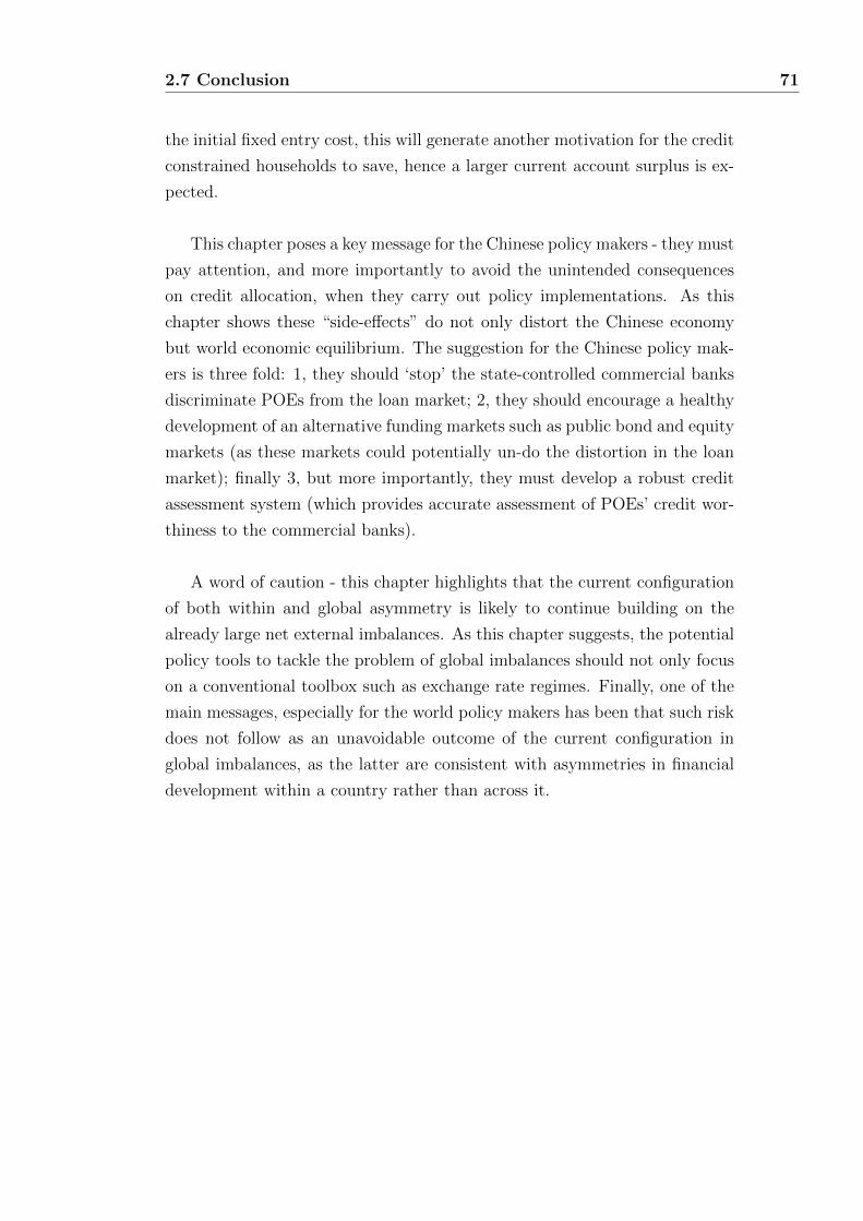
2.7 Conclusion 71
the initial fixed entry cost, this will generate another motivation for the credit
constrained households to save, hence a larger current account surplus is ex-
pected.
This chapter poses a key message for the Chinese policy makers - they must
pay attention, and more importantly to avoid the unintended consequences
on credit allocation, when they carry out policy implementations. As this
chapter shows these “side-effects” do not only distort the Chinese economy
but world economic equilibrium. The suggestion for the Chinese policy mak-
ers is three fold: 1, they should ‘stop’ the state-controlled commercial banks
discriminate POEs from the loan market; 2, they should encourage a healthy
development of an alternative funding markets such as public bond and equity
markets (as these markets could potentially un-do the distortion in the loan
market); finally 3, but more importantly, they must develop a robust credit
assessment system (which provides accurate assessment of POEs’ credit wor-
thiness to the commercial banks).
A word of caution - this chapter highlights that the current configuration
of both within and global asymmetry is likely to continue building on the
already large net external imbalances. As this chapter suggests, the potential
policy tools to tackle the problem of global imbalances should not only focus
on a conventional toolbox such as exchange rate regimes. Finally, one of the
main messages, especially for the world policy makers has been that such risk
does not follow as an unavoidable outcome of the current configuration in
global imbalances, as the latter are consistent with asymmetries in financial
development within a country rather than across it.
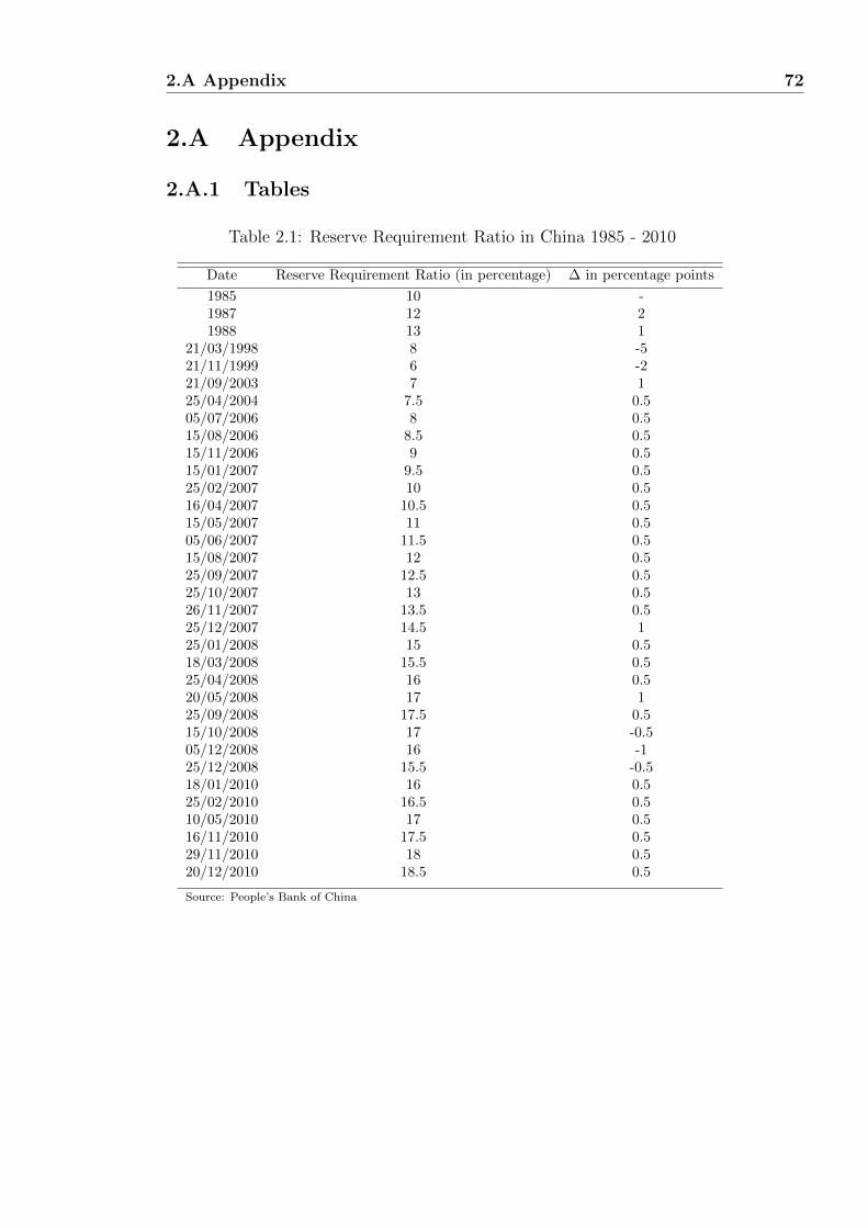
2.A Appendix 72
2.A Appendix
2.A.1 Tables
Table 2.1: Reserve Requirement Ratio in China 1985 - 2010
Date Reserve Requirement Ratio (in percentage) ∆ in percentage points
1985 10 -1987 12 21988 13 1
21/03/1998 8 -521/11/1999 6 -221/09/2003 7 125/04/2004 7.5 0.505/07/2006 8 0.515/08/2006 8.5 0.515/11/2006 9 0.515/01/2007 9.5 0.525/02/2007 10 0.516/04/2007 10.5 0.515/05/2007 11 0.505/06/2007 11.5 0.515/08/2007 12 0.525/09/2007 12.5 0.525/10/2007 13 0.526/11/2007 13.5 0.525/12/2007 14.5 125/01/2008 15 0.518/03/2008 15.5 0.525/04/2008 16 0.520/05/2008 17 125/09/2008 17.5 0.515/10/2008 17 -0.505/12/2008 16 -125/12/2008 15.5 -0.518/01/2010 16 0.525/02/2010 16.5 0.510/05/2010 17 0.516/11/2010 17.5 0.529/11/2010 18 0.520/12/2010 18.5 0.5
Source: People’s Bank of China

2.A Appendix 73
Table 2.2: Open Market Operations in China 2000 - 2006
Year Total Reserve Repos Repos Central Bank Bills
2000 132 107 25 02001 50 26 24 02002 77 45 32 192003 73 6 18 492004 138 1 43 942005 189 3 62 1242006 137 1 39 98
Total 796 189 243 384Note: This table shows number of OMOs within a year.Source: People’s Bank of China
Table 2.3: Issuance of Central Bank Bill in China 2000 - 2009
Year Size of Central Bank Bill (RMB 100m)
2000 02001 02002 1937.52003 7226.82004 17037.342005 278222006 36573.812007 40721.282008 429602009 39740Source: People’s Bank of China

2.A Appendix 74
2.A.2 Figures
Figure 2.12: Ease of Doing Business Index

2.A Appendix 75
Figure 2.13: Productivity Comparison between SOEs and POEs Across 28Manufacturing Industries in China
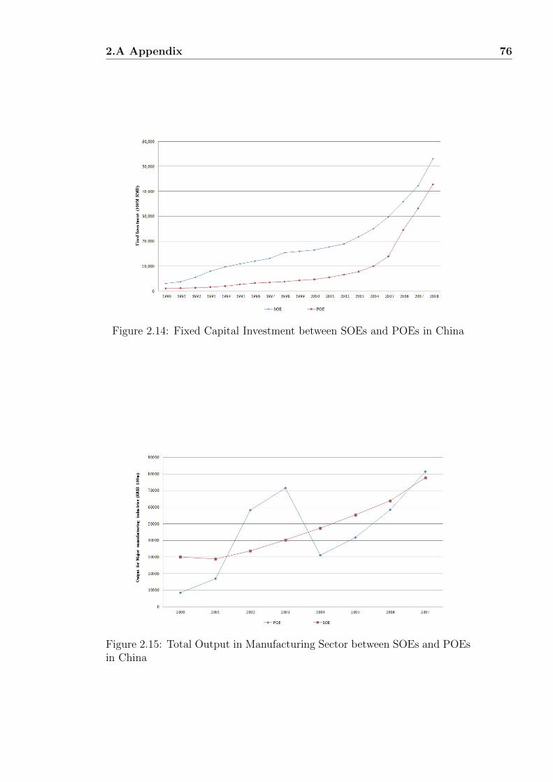
2.A Appendix 76
Figure 2.14: Fixed Capital Investment between SOEs and POEs in China
Figure 2.15: Total Output in Manufacturing Sector between SOEs and POEsin China
2.A Appendix 77
Figure 2.16: Differences Between SOEs’ and POEs’ Syndicated Loan Issuancein China
Figure 2.17: Differences between SOEs’ and POEs’ Bond Issuance in China
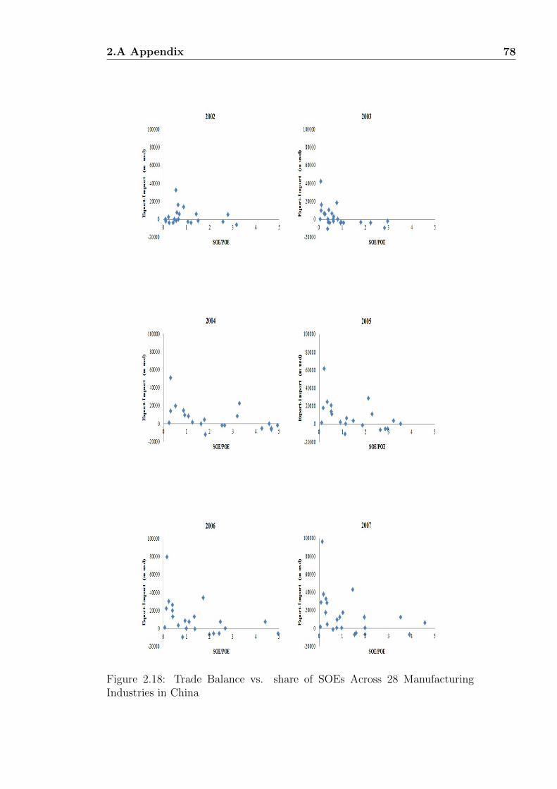
2.A Appendix 78
Figure 2.18: Trade Balance vs. share of SOEs Across 28 ManufacturingIndustries in China
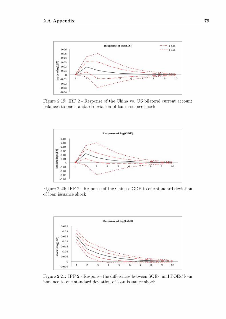
2.A Appendix 79
Figure 2.19: IRF 2 - Response of the China vs. US bilateral current accountbalances to one standard deviation of loan issuance shock
Figure 2.20: IRF 2 - Response of the Chinese GDP to one standard deviationof loan issuance shock
Figure 2.21: IRF 2 - Response the differences between SOEs’ and POEs’ loanissuance to one standard deviation of loan issuance shock

2.A Appendix 80
Figure 2.22: Equilibrium Path after a Borrowing Ability Shock

2.A Appendix 81
Figure 2.23: Trend vs. No-Trend - 1
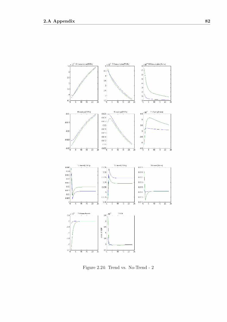
2.A Appendix 82
Figure 2.24: Trend vs. No-Trend - 2
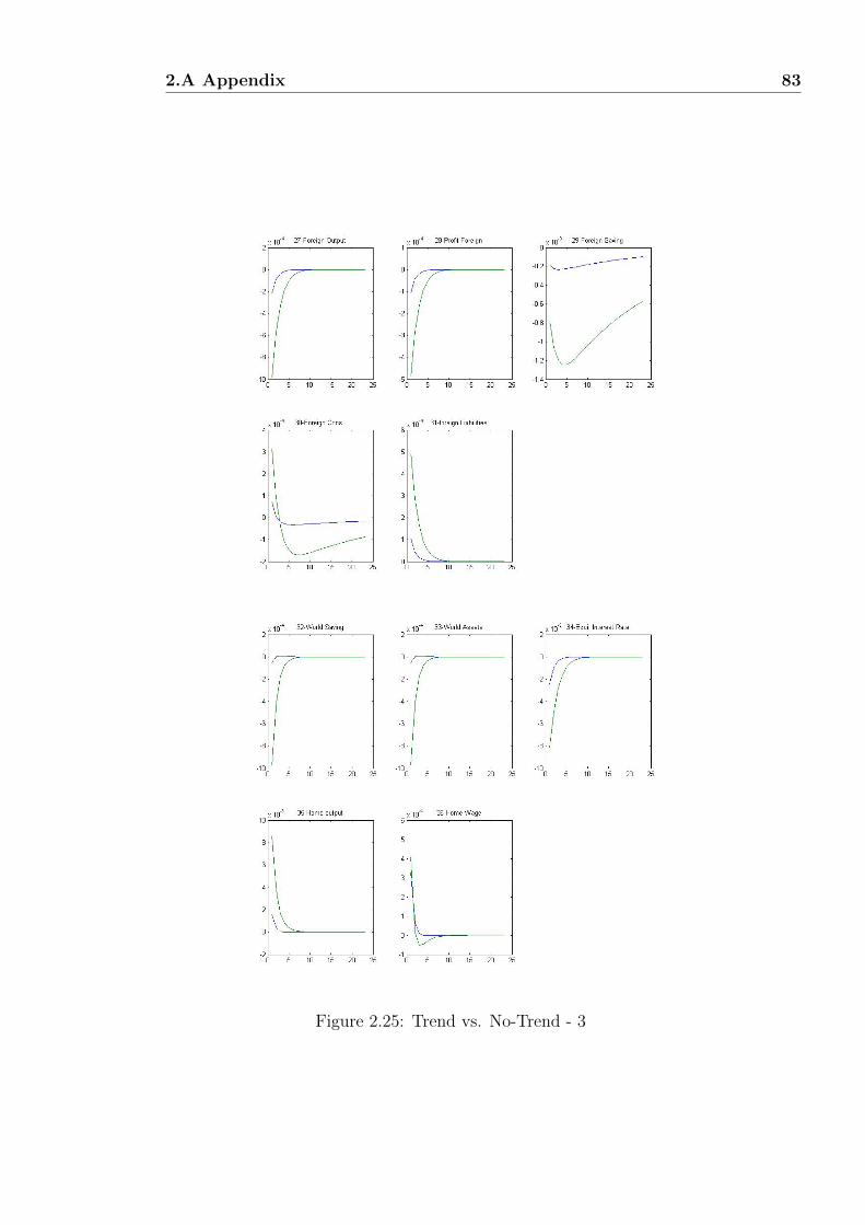
2.A Appendix 83
Figure 2.25: Trend vs. No-Trend - 3

2.A Appendix 84
Figure 2.26: 3 Cases - 1

2.A Appendix 85
Figure 2.27: 3 Cases - 2

2.A Appendix 86
Figure 2.28: 3 Cases - 3

Chapter 3
Causes of Asset Shortages in
Emerging Markets
3.1 Introduction
Capital markets in emerging markets (EMs) have expanded rapidly in recent
years, with demand for assets expected to grow strongly for the foreseeable
future. Following the 1980s crisis in Latin America and the 1990s crisis in
East Asia, most EMs undertook bold reforms, encompassing fiscal ortho-
doxy, predictable monetary policies, and other structural reforms that led to
a strengthening of the balance sheets of both the public and private sectors.
The ensuing macroeconomic stability was not materially affected by the 2008
global credit crisis, with macroeconomic stability remaining intact and bal-
ance sheets still robust. Rising domestic savings - in the form of increasingly
capitalized pension and mutual funds and reduced financing needs of public
entities - and the increasing demand for EMs assets from local and foreign
investors, insurance companies, and other financial intermediaries, have led
to greater appetite for domestic equity, bonds, and other financial assets.
The paradox of the improved macroeconomic environment in EMs is that
while savings have remained strong or even increased, the supply of financial
assets has not risen commensurately. High equity returns, a stable macroeco-
nomic environment and increasing assets under management by institutional
investors have not led to the takeoff of the primary market in most EMs.
Equity issuances/Initial Public Offerings (IPOs) are still infrequent, though
there are regional variations (Figure 3.4). Whereas Asian companies tend to
issue domestically, Latin American companies are biased toward raising capi-

3.1 Introduction 88
tal overseas instead. Most domestic fixed income markets are highly underde-
veloped and dominated by public debt; outside public short-term debt, most
fixed-income products remain illiquid (de la Torre and Schmukler (2006)).
The constraint to expanding domestic assets is partly structural, related
to market size. Outside the Brazil, Russia, India, and China (BRICs), most
EMs are small economies, which limits the scope for deep domestic financial
markets. The selective nature of issuers - mainly companies in the mining
sector in Latin America or manufacturing companies in East Asia - restricts
the benefit of diversification for investors. Corporate culture, such as the un-
willingness to give up control, also plays a part in explaining why entities and
controlling shareholders are reluctant to relinquish control over firms.
The lack of domestically investible assets, if not addressed, could poten-
tially lead to large macroeconomic imbalances that threaten stability. A short-
age of investible assets leads to excess liquidity that lowers interest rates and
raises asset prices on equity and housing. Moreover, the dominance of buy
and hold investors leads to fewer transactions, which raises the entry and exit
costs into the stock market. In any case, share prices are not good indicators
of actual market prices in illiquid and underdeveloped markets. They suffer
from a shortage of information and high spreads, and are prone to be affected
by noise traders and large swings in price volatility. The shortage of domestic
financial assets, combined with investment restrictions abroad, could lead to
bubbles with too much capital chasing too few assets. Market efficiency is
also affected, as in a world of imperfect capital mobility - owing to investment
restrictions misalignments in asset valuation relative to the economic funda-
mentals can be long lasting.
The chapter is structured as follows. In Section II, we describe asset short-
ages and their symptoms; in Section III, we discuss possible causes of asset
shortages. The asset shortage index is constructed in Section IV, followed in
Section V by an estimation of the factors driving asset shortages. Section VI
concludes with policy implications.
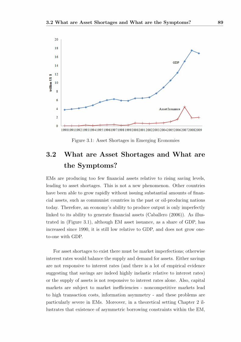
3.2 What are Asset Shortages and What are the Symptoms? 89
Figure 3.1: Asset Shortages in Emerging Economies
3.2 What are Asset Shortages and What are
the Symptoms?
EMs are producing too few financial assets relative to rising saving levels,
leading to asset shortages. This is not a new phenomenon. Other countries
have been able to grow rapidly without issuing substantial amounts of finan-
cial assets, such as communist countries in the past or oil-producing nations
today. Therefore, an economy’s ability to produce output is only imperfectly
linked to its ability to generate financial assets (Caballero (2006)). As illus-
trated in (Figure 3.1), although EM asset issuance, as a share of GDP, has
increased since 1990, it is still low relative to GDP, and does not grow one-
to-one with GDP.
For asset shortages to exist there must be market imperfections; otherwise
interest rates would balance the supply and demand for assets. Either savings
are not responsive to interest rates (and there is a lot of empirical evidence
suggesting that savings are indeed highly inelastic relative to interest rates)
or the supply of assets is not responsive to interest rates alone. Also, capital
markets are subject to market inefficiencies - noncompetitive markets lead
to high transaction costs, information asymmetry - and these problems are
particularly severe in EMs. Moreover, in a theoretical setting Chapter 2 il-
lustrates that existence of asymmetric borrowing constraints within the EM,
3.2 What are Asset Shortages and What are the Symptoms? 90
leads to supply of financial asset can not match up with the rate of demand
increases, as a result asset shortages emerges.
Prior to the emerging market crises of the 1990s, EMs grew rapidly, with
high savings rates accompanied by high investment rates. However, while
savings rates have remained high, investment rates have started to decline
following the Asian crisis, leading to a shortage of financial assets in these
countries (Rajan (2006)). The shortage was exacerbated by the rapid growth
of savings in China and in commodity producing countries that do not gener-
ate financial assets on a sufficient scale to satisfy demand for them (Caballero,
Farhi, and Gourinchas (2006)).
Fewer investment opportunities in EMs have resulted in asset shortages,
with negative implications for both the macroeconomy and financial markets.
Investment opportunities have been restrained by the inability to issue finan-
cial assets in EMs. Emerging bottlenecks in capital markets, with too much
money chasing too few assets, have given rise to some perverse consequences
for market efficiency. These include:
• Low real interest rates. With too much savings chasing too few invest-
ments, real interest rates are kept low (by historical standards) (see also
GFSR (2012)). Low interest rates are in turn pushing economic agents
into higher-risk assets, searching for yields and bringing real interest
rates down further.
• Illiquid capital markets in EMs. The lack of liquidity in many EM
capital markets is a result of investors trying to grab any assets they
can and holding on to them. The mismatch leads to buy and hold
strategies by investors and concentrated ownership, leading to illiquidity
in domestic capital markets (and lending itself to market misconduct
and price manipulation).
• Misalignment in the valuation of assets, leading to bubbles in extreme
cases. A mismatch between asset supply and demand may lead to sus-
tained misalignments in asset valuation relative to the economic funda-
mentals. The recurrent speculative bubbles observed in EM economies
are a reflection of these misalignments1.
1While only anecdotal, the last few decades have seen increases in bubbles, which havebecome more frequent across more financial assets. Mexican and other Latin Americandebt suffered from a crash in 1982 and again in 1994; stocks of the Asian Tiger economies

3.3 What Causes Asset Shortages? 91
• Capital flows from EMs to advanced economies (AEs). The Lucas para-
dox, that capital is flowing from EMs to advanced countries, is again a
symptom of asset shortages in EMs. With a limited amount of assets to
invest in, savers in EMs invest their savings overseas. Sovereign Wealth
Funds (SWFs) are an extreme form of asset shortage, with massive sav-
ings in EMs not absorbed by the domestic economy, because of the lack
of financial assets.
3.3 What Causes Asset Shortages?
Asset shortages have become severe in the last two decades in EMs, owing to
a combination of (i) the dwindling supply of financial assets; (ii) the increased
supply of domestic savings; (iii) regulatory restrictions; and (iv) other factors.
Let us look at them in turn.
3.3.1 Dwindling Supply of Financial Assets in EMs
• Fiscal improvements. Government fiscal policy is a key source of the
supply of financial assets. According to the ‘Original Sin’ line of rea-
soning (Eichengreen and Hausmann (1999); Hausmann and Panizza
(2010)), most EM governments and corporations are unable to bor-
row in local currency, due to shallow domestic capital markets and the
unwillingness of investors to fund large investments in an EM currency,
with the side effect of leading to a lack of supply of domestic financial
assets. Several EM countries have improved their overall sovereign debt
management practices, by increasing the share of domestic-currency de-
nominated debt. Nonetheless, although the issuance of domestic debt
has recently increased thereby raising the supply of domestic financial
assets, the original sin has declined only marginally and only in a few
countries (Hausmann and Panizza (2010)). Given original sin, absti-
nence of debt has become an important strategy in EMs, with govern-
ments running orthodox fiscal policies, thereby supplying few financial
assets.
came back to earth in 1997; China, and with it commodity prices, peaked in 2007, andprices have fallen since, before recovering more recently. EM stock, currencies, credit, andother commodities once operated in their separate kingdoms and followed their own rules.Now, given asset shortages, they increasingly are interlinked financial assets; and when onemarket expands with the inflow of money, many risky assets shoot upward simultaneously,forming synchronized bubbles.
3.3 What Causes Asset Shortages? 92
• High uncertainty. EMs have been subject to severe and repeated shocks
in the last two decades, most notably the Asian crisis, which created high
risk averseness. Banking systems in Asia and Latin America have been
highly regulated since, forced to keep high liquidity buffers and capital
ratios, which has created a stable banking system, though also a conser-
vative one often constraining credit growth. In addition, poor property
rights, weak contract enforcement, and judicial arbitrariness are just a
few problems that by increasing uncertainty, constrain investment and
lead to low private rates of return (owing to low appropriability). While
most EMs have made great progress in addressing these problems over
time, this has not been enough to address asset shortages2.
3.3.2 Increased Supply of Domestic Savings
• Pension reforms in Latin America, increasing commodity prices in the
Middle East and Africa, and rising savings in East Asia have contributed
to an increasing supply of savings in EMs. While one could have ex-
pected rising consumption levels and falling savings with rising income
per capita, pension reforms and positive exogenous shocks in the form
of rising commodity prices or rising demand for export products have
tended to lead to high saving rates.
• Underdeveloped capital markets. Savings in EMs are motivated in part
to fund lumpy physical investments, because underdeveloped capital
markets require agents to save on a massive scale and over an extended
period of time. As EMs industrialize, and as investment requirements
increase substantially, credit constrained investors require ever larger
savings to finance lumpy investments. Investors have to accumulate a
large share of the savings before they can ever invest, leading to an
increase in domestic savings.
3.3.3 Regulatory Restrictions
• Regulatory restrictions on agents. A substantial portion of the world’s
desired savings are put to work by governments, central banks, and fi-
2Past investment excesses. One argument, advanced by Rajan (2006), is that past boomsare still working themselves through the system. Following past over-investment, the in-vestment overhang still needs some time to pass through the system. In other words, pastmis-allocations of investment are still haunting current investment expenditure. Corpora-tions are therefore cautious in their investment strategy to avoid over-investment. Whilethere is some plausibility to this argument, it is a temporary phenomenon.

3.3 What Causes Asset Shortages? 93
nancial institutions like insurance companies. Many of these agents are
ordered by law to buy fixed-income products, such as domestic govern-
ment bonds, and are constrained in regard to investments in certain
assets classes, including foreign assets.
Regulatory Restrictions of Latin American Pension Funds
Chile3 was the pioneer in pension reform in Latin America, and its
model was copied throughout Latin America. In 1981, a comprehen-
sive change took place in the pension system, changing the state-run,
defined-benefit scheme to a defined-contribution system managed en-
tirely by the private sector (by pension management companies called
“AFPs”), under the supervision of a dedicated government agency, the
Superintendency of AFP. Chile introduced mandatory individual sav-
ings accounts in the early 1980s; later, Argentina, Bolivia, Colombia,
Ecuador, Mexico, Peru, and Uruguay followed suit, borrowing heavily
on the Chilean model (Borensztein, Cowan, Eichengreen, and Panizza
(2008)).
The system’s investment opportunities are heavily regulated. The reg-
ulator of pension funds in all these Latin American countries sets strict
regulations on foreign exposure, ranging from single-digit limits to about
one-third of the funds. Both foreign and domestic fixed income in-
vestments typically are restricted to high-grade entities, funds for the
government, and local blue-chip companies. Exposure to equity is also
highly restricted, again only to blue-chip companies. Pension fund in-
vestments have given rise to abnormally low corporate bond spreads,
well below sovereign spreads. The upward trend in stock prices is at-
tributed partly to the demand exerted by these pension funds. This
brings about some perverse consequences for market efficiency: prices
may become misaligned from fundamentals; and liquidity is continually
drained from the market place.
Restricting investment opportunities for pension funds reduces the in-
vestment universe. The limits might have been set on the grounds that
(i) pension funds should rejuvenate anemic local financial markets; (ii)
emerging markets are financially constrained and hence should not be
3See Table 3.3, 3.4, 3.5, 3.6, 3.7 and 3.8

3.3 What Causes Asset Shortages? 94
capital exporters; and (iii) pension fund managers and supervisors are
unfamiliar with external investment opportunities, exacerbating portfo-
lio risk and moral hazard. These motives increasingly do not hold sway,
and if not reformed, could lead to rising asset shortages. First, the
overarching goal of any funded pension system is to maximize old-age
retirement wealth at tolerable risk levels. This goal should not be sub-
ordinated to other commendable objectives. Local markets are poorly
correlated with international markets, thus diversification is likely to
pay off in the long term. Second, for crisis prone economies, domestic
systemic risk makes it advisable to partially rely on more stable mar-
kets, provided efficient risk management policies are in place in every
AFP. Finally, it is not necessary for the pension fund manager to deal
with foreign asset selection directly, because many reputable interna-
tional global fund managers with excellent track records can be hired
at low cost, as they are in many countries.
The limit on foreign investment and risky domestic investable securities
could be further relaxed from the current levels to reduce asset short-
age problem. There is strong evidence internationally that home bias
tends to result in strong sub-optimality of portfolios. Thus, it is not
possible to justify a limit on foreign investment on economic grounds.
Ideally, limits should be lax enough to allow AFPs to use less restrictive
risk management policies and to eliminate the apparent excess demand
for local financial instruments. Public offerings have not shown the ex-
pected dynamism and have largely lost their desirable characteristics
(efficient pricing and liquidity). Asset-backed securities on mortgages
and other receivables, real estate, and infrastructure projects should be
given priority.
• Regulation restricting supply of risky financial assets. Many EMs (e.g.,
China) do not allow issuance of high-yield debt or other non-plain vanilla
financial assets. This prevents the development of a whole asset class
in such countries, thereby restricting the supply of financial assets.
• Asymmetric financial markets. As argued in Chapter 2, policy inter-
ventions (or its unintended consequences see Chapter 2) which favor
(or discriminate) a certain set of firms in accessing to domestic credit
market can distort the equilibrium between demand and supply of the
financial assets. In particular these policies reduce the ability of asset

3.4 Asset Shortage Index 95
supplier in issuing financial assets, lead to asset shortages in domestic
economy.
3.3.4 Other Reasons for Asset Shortages in EMs
• Home bias (for political reasons). While investors in EMs often are keen
to invest their assets overseas as a store of value, worsening macroeco-
nomic conditions of advanced economies in recent years, compared to
EMs, has made it increasingly risky to invest in these regions, as epit-
omized by the recent crisis. Also, from the Balassa-Samuelson effect4,
we know that EMs should expect their real equilibrium exchange rate
(REER) to appreciate over time, meaning that overseas investment in
AEs will be subject to capital losses arising from exchange rate appreci-
ation. Finally, the investments of Middle Eastern and Chinese investors
in AEs are being increasingly scrutinized, thereby creating considerable
uncertainty (as epitomized by the failure of Dubai World and CNOOC
to acquire Western assets owing to political opposition). Such uncer-
tainty has made investment overseas less attractive, thereby reducing
access to an important asset class.
• Increasing appetite for EM assets by AEs. As part of portfolio diver-
sification, advanced country portfolio managers have been increasingly
investing part of their portfolios in EMs, thereby reducing the supply
of domestic financial assets available to EM domestic investors.
3.4 Asset Shortage Index
We define our asset shortages index by capturing the difference between de-
mand and supply for financial assets. Domestic demand for assets (latent
asset demand) is proxied by gross domestic savings (i.e. all the resources
available to invest), while the supply of financial assets is defined as domestic
issuance of bonds, loans, and equity, as well as the net purchase of foreign as-
sets and domestic assets by foreign investors. In addition, the change in short
term deposits also is considered to be adding to the supply of financial asset,
because it reflects the temporary parking of funds, which could be motivated
4The Balassa-Samuelson effect postulates that if the productivity growth differentialbetween the traded and non-traded goods sectors is larger in the developing countries thanin advanced ones, then the relative price of non-traded to traded goods will be rising fasterin the developing than in advanced countries, leading to an exchange rate appreciation.

3.4 Asset Shortage Index 96
by a willingness to hold liquid assets as a precaution.
The supply of financial asset is modeled in the same spirits as discussed in
other chapters of the current thesis as well as in Caballero, Farhi, and Gour-
inchas (2008). Broadly speaking these papers defined the supply of financial
asset as Vt = δPVt , where PVt denote the present value of the economy’s
future output, and the parameter δ represents the share of PVt that can be
capitalized today and transformed into a tradable asset hence the total asset
issued in domestic economy. The δ parameter captures the level of financial
development in an economy, intuitively for a given level of future output, a
higher δ implies domestic agent (enterprise, government or household) can
borrow more against their future income, this is equivalent as saying agents
can issue more financial assets (Bond, Equity and Loans).
To estimate our asset shortages (AS) index, we use the following formula:
AS = 1−(B + E + L+ ∆S.D.+NPFA
S
)(3.1)
where S=domestic national savings, B=bond issuance in the domestic
market, E=equity issuance in the domestic market, L=loan issuance in the
domestic market, and S.D.= short term deposits. NPFA= net purchase of
foreign financial assets by domestic residents, which reflects the position of do-
mestic investors’ holdings of foreign assets (debt, equity, financial derivatives
and other investments) minus the net position of foreign investors’ holdings
of domestic assets. The sum of B + E + L + ∆S.D. + NPFA is therefore a
reflection of the supply of financial assets.
3.4.1 Flow of Funds of Assets
Figure 3.2 illustrates the foundation of the asset shortage index, in which
household savings is being invested in either liquid or non-liquid financial
assets. On the demand side, enterprises, government and households issue
new loans, bonds, or equity to finance their real investment project (or con-
sumption), ranging from a new mortgage to a new enterprise. Alternatively,
they finance projects either by reducing short-term assets or through foreign
borrowing. According to the system of national accounts, the national finan-
cial account comprises seven categories of investment assets: (1) monetary
gold; (2) currency and deposits; (3) securities other than shares; (4) loans;
(5) shares and other equity; (6) insurance technical reserves; and (7) other

3.4 Asset Shortage Index 97
Figure 3.2: Flow of Fund
accounts receivable. In our asset shortage index, we have captured the cur-
rency and deposits, loans, and shares and other equity. The remaining terms,
for the purposes of the AS-Index are unlikely to be significant. For example,
monetary gold is mainly an investment option for the central banks. Also, the
level of monetary gold reserves in the central bank does not vary from year
to year, so in the overall economy monetary gold has very little relevance to
asset shortages. Insurance technical reserves are very small in EMs, and data
limitations made it impossible to include it in our index. Other accounts re-
ceivable is in general small in EMs; limited and underdeveloped credit ratings
data make it difficult for companies to assess the risk of lending. Moreover,
the duration of such a transaction is very short, limiting its importance.
3.4.2 Construction of the Index
Using available data, the asset shortage index for 41 EMs was constructed
from 1995 - 20085. Depending on the issuing country and issuing market, we
5The EMs are Argentina, Brazil, Chile, Colombia, Mexico, Panama, Peru, Venezuela,China, Hong Kong, India, Indonesia, Korea, Malaysia, Philippines, Taiwan, Thailand,Vietnam, Bahrain, Egypt, Israel, Kazakhstan, Kuwait, Morocco, Pakistan, Saudi Arabia,

3.4 Asset Shortage Index 98
combined a number of databases to obtain the most comprehensive data set
that is consistent across countries. The variables used to construct the Asset
Shortage Index are as follows:
• Gross national savings. The data for gross national savings reflect
gross national disposable income subtracted by total expenditure; it
represents economic resources available for investment. The dataset on
gross domestic savings was obtained from the World Development Index
(WDI) or was constructed from the World Economic Outlook (WEO)
when WDI data were not available.
• Bond, equity, and loan issuance. Dealogic records all the domestic is-
suances of bonds, equity and syndicated loan. In this chapter, as a
starting point, we use syndicated loan data as a proxy for the total loan
issuance6 because: 1, it is already difficult to obtain gross loan issuance
data for advanced economies and this task became ‘mission impossible’
in EMs; 2, a series of recent papers have emerged, which use syndicated
loan issuance data to study the properties of the loan market (i.e. Sufi
(2007)); 3, the short term deposit is included as part of the asset supply
which reflects large share of the unaccounted (by syndicated loan) gross
loan issuance. For each country, the bond, loan and equity issuances
were aggregated for each year.
• Net purchase of foreign financial assets. In an open economy, when
a domestic resident purchases assets overseas (debt, equity, financial
derivative, other investments), it represents an increase in the supply
of financial assets for the domestic investor. Similarly, when a for-
eigner buys domestic assets, this is equivalent to a reduction in domes-
tic financial assets available to domestic investors. Foreign institutional
investors’ interest in emerging markets has surged in recent years, be-
cause of improved sovereign liability management, resulting in a secular
increase in demand for both external and local EM asset classes. In-
creases in privatization, improvements in investment climate, and easing
of capital account regulations, resulting in a rapid rise in the share of
the investable portion of the local equity market, have also attracted
South Africa, Turkey, UAE, Bulgaria, Croatia, Czech Republic, Hungary, Latvia, Lithua-nia, Poland, Romania, Russia, Slovak Republic, Slovenia, Ukraine.
6As a robustness check, we also used loan stock data (from Bankscope) to constructa proxy for gross loan issuance, the implied asset shortage index is ‘similar’ to the oneconstructed using syndicated loan data therefore they are not reported in the currentchapter.

3.4 Asset Shortage Index 99
foreign institutional investor participation. Data for net purchase of
foreign financial assets are obtained from balance of payment statistics.
• Change in short-term deposits. Part of an economic agent’s assets is
parked in short-term deposits, as a precaution against uncertainty, for
instance. Investors can temporarily park funds as short-term deposits,
creating a temporary investment vehicle. Data for short-term deposits
are obtained from Bankscope, which aggregates all the banks’ balance
sheets to construct short-term deposits in an economy.
It is clear from the asset shortage index that, in recent years, asset short-
age has become a rising issue in EMs, with few countries left out (Figure 3.3).
The four snapshots 1996, 2000, 2005, and 2008 indicate that asset shortage is
a general EM problem, with slight regional variations (e.g., the Middle East,
which benefited from the oil windfall, and East Asia, which benefited from
the manufacturing boom) and with some variations over time.
Issuance of financial assets has been on an upward trend regionally - un-
til the recent crisis - but with low levels relative to GDP (negative numbers
mean that the reduction in cash deposits outweighs issuance of bonds, equity,
and loans). Regional variations are striking. East Asia, the Middle East,
and Africa appear to have the highest issuance of financial assets, while Latin
America and Eastern Europe lag behind (Figure 3.4).
Bond and syndicated loan issuance has been the principal source of finan-
cial assets in EMs, with equity issuance starting only in the mid-2000s. While
the Asian crisis has dented some of the supply of bonds, in the last decade
there has been a rise in both domestic bond issuance and syndicated loan is-
suance, though the latter has seen a sharp fall during the global crisis. Equity
issuance, on the other hand, started growing rapidly only in 2005, from very
low levels, and was negatively affected by the crisis. Net purchase of foreign
financial assets, while initially positive, has turned negative in recent years as
domestic investors have started to pick up foreign financial assets, suggesting
that foreigners are buying relatively more domestic financial assets (Figure
3.5, 3.7, 3.6, 3.8 and 3.9).
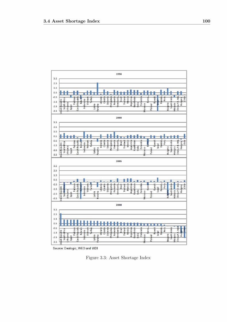
3.4 Asset Shortage Index 100
Figure 3.3: Asset Shortage Index

3.5 Empirical Estimation 101
3.5 Empirical Estimation
3.5.1 Methodology
We will proceed by estimating the determinants of the asset shortage (AS)
index. In macroeconomic panel regressions, various estimation issues are en-
countered that must be addressed to make appropriate inferences. The first
major hurdle is the omitted variables bias, which can lead to possible corre-
lation between the regressors and the error term. Second, two-way causality
between the dependent variable and the explanatory variables is likely to be
present, which leads to inconsistent estimators. The third problem specific to
dynamic panels is the “dynamics panel bias”, from the inevitable correlation
between the lagged dependent variable and country-specific fixed effects (Al-
varez and Arellano (2003)).
System-GMM is used instead to carry out the estimations (Arellano and
Bover (1995) and Blundell and Bond (1998)). While it still might suffer from
weak instrument bias, it provides consistent and more efficient estimators.
It reduces the bias by incorporating more moment conditions, with these
additional moment restrictions also being tested. The regressions are run on
first-difference and not on levels, owing to concerns about trending variables
and unit root. The test statistics indicate that the instruments are valid7,
and that there is no serial correlation in the error term, which allows us to
carry on with the system-GMM method. We can therefore proceed with the
following estimation (results are in Table 3.1):
AssetShortageIndexit = β1ASIndexit−1 + β2ln(∆GDPit)
+ β3Inflationit + β4∆RealInterestRateit
+ β5CountryCreditRatingit−1 + β6d.f.Ex.Rateit−1
+ β7GovtF iscalBalanceit−1 + β8Govt.Stabilityit
+ β9WorldGDPGrowthit + β10X + εit (3.2)
with the countries defined in Table 4.10, the key variable and their sources
in Table 4.11, 4.12, 4.13, 4.14 and 4.15. The variables were chosen on theo-
7We noticed that the Arellano-Bond test statistics are ‘too’ high in some of the regres-sion specifications, which poses potential problem - invalidity of the instruments, howeverpanel fixed effect estimations are also implemented in parallel as robustness check. Theresults are similar between two estimation procedures moreover, estimation results on othervariables are consistent with the existing literature therefore we believe the results fromGMM estimations reflect the true estimates with certain degree of consistency.

3.5 Empirical Estimation 102
retical grounds (see below).
3.5.2 Key Findings
There is strong evidence of asset shortage persistence. An asset shortage in
the previous period has a negative impact on asset shortages in the current
period, with significance at the 1 percent level. This implies that the imbal-
ance between asset supply and asset demand is not being addressed rapidly
by capital markets, which could reflect impediments to asset creation.
Government stability is found to reduce the AS index. Across the various
specifications, some statistically significant evidence shows that as govern-
ment stability improves - presumably leading to a more stable investment
climate - investors might be more willing to supply financial assets because
uncertainty is diminished. If openness and change in GDP per capita are
added as additional variables in the regression, the explanatory power of gov-
ernment stability is reduced - probably because of their co-linear relationship
with this variable.
GDP growth worsens the AS index, confirming that economic growth and
supply of financial assets do not grow together. The coefficients are significant
across all the different specifications, confirming that the issuance of financial
assets is not dependent on economic growth per se. A country can therefore
grow despite limited financial assets.
A stable macroeconomic environment proxied by low inflation encourages
the issuance of financial assets, because it reduces the level of risk, though
the statistical significance of this variable is not always strong.
A country’s credit rating has no significant power in explaining asset short-
ages. This means investors are less concerned about a country’s credit rating
when making investment decisions.
Change in real interest rates is not statistically significant in explaining
the AS index, suggesting that interest rates do not act as an equilibrium force
between supply and demand for assets in EMs. Under the incomplete market
setting that characterizes EMs, this is to be expected, because savings and
the supply of financial assets do not necessarily respond rapidly to interest

3.5 Empirical Estimation 103
Tab
le3.
1:Syst
emG
MM
Reg
ress
ion
Outp
ut
for
Mac
roec
onom
icV
aria
ble
sE
xpla
nat
ion
ofth
eIn
dex
Asset
Sh
ortage
In
dex
In
dep
en
dent
varia
ble
s(1)
(2)
(3)
(4)
(5)
(6)
(7)
(8)
(9)
A.S
.In
dex
(t-1)
0.2
89***
0.2
66***
0.2
62***
0.2
92***
0.2
80***
0.2
83***
0.2
93***
0.2
85***
0.2
88***
(0.0
46)
(0.0
41)
(0.0
72)
(0.0
46)
(0.0
48)
(0.0
49)
(0.0
45)
(0.0
47)
(0.0
51)
Log
∆G
DP
0.0
577**
0.0
63**
0.0
74
0.0
58*
0.0
52*
0.0
75**
0.0
68**
0.0
61**
0.0
57**
(0.0
282)
(0.0
28)
(0.0
48)
(0.0
28)
(0.0
26)
(0.0
28)
(0.0
29)
(0.0
28)
(0.0
27)
In
flatio
n0.0
433
0.0
48
0.0
69
0.0
46
0.0
45
0.0
49
0.0
43
0.0
47
0.0
42
(0.0
330)
(0.0
34)
(0.0
52)
(0.0
33)
(0.0
34)
(0.0
34)
(0.0
32)
(0.0
33)
(0.0
31)
∆R
eal
interest
rate
-0.0
0748
-0.0
12
0.0
04
-0.0
03
-0.0
08
-0.0
09
-0.0
04
-0.0
06
-0.0
08
(0.0
167)
(0.0
18)
(0.0
16)
(0.0
15)
(0.0
17)
(0.0
17)
(0.0
17)
(0.0
17)
(0.0
17)
Cou
ntrys
credit
ratin
g-0.0
976
-0.0
32
-0.0
71
-0.1
03
-0.0
74
-0.0
83
-0.0
63
-0.1
00
-0.0
96
(t-1)
(0.0
691)
(0.0
82)
(0.0
89)
(0.0
71)
(0.0
83)
(0.0
70)
(0.0
73)
(0.0
67)
(0.0
69)
De
facto
exch
an
ge
rate
0.0
467
-0.0
06
-0.0
49
0.0
47
0.0
37
0.0
46
0.0
41
0.0
45
0.0
49
(t-1)
(0.0
896)
(0.0
82)
(0.1
57)
(0.0
92)
(0.0
91)
(0.0
90)
(0.0
89)
(0.0
89)
(0.0
85)
Govern
ment
fiscal
bal.
1.6
20*
0.5
74
1.8
78
1.6
90*
1.4
27
1.6
57*
1.3
20
1.8
49**
1.5
44*
(t-1)
(0.9
17)
(1.1
66)
(1.2
58)
(0.9
33)
(0.9
44)
(0.8
98)
(0.9
38)
(0.8
46)
(0.9
01)
Govern
ment
stab
ilit
y-0.1
05*
-0.0
89
-0.1
30
-0.1
07*
-0.0
98*
-0.1
07*
-0.1
11*
-0.1
03*
-0.1
04*
(0.0
590)
(0.0
62)
(0.0
80)
(0.0
59)
(0.0
56)
(0.0
59)
(0.0
59)
(0.0
59)
(0.0
56)
World
GD
Pgrow
th
-4.7
28*
-4.8
49*
-4.1
32
-4.5
80*
-4.7
61*
-6.3
31**
-5.4
00**
-4.6
01*
-4.7
65*
(2.3
96)
(2.3
88)
(2.7
19)
(2.4
23)
(2.3
56)
(2.6
18)
(2.4
45)
(2.3
86)
(2.4
68)
Op
enn
ess
(t-1)
-0.0
04*
(0.0
02)
Log
∆G
DP
-0.0
43
per
cap
ita
(t-1)
(0.0
64)
Cris
isd
um
my
(t-1)
-0.5
70**
(0.2
15)
Regio
nal
du
mm
y0.1
65
(L
atin
Am
eric
a)
(0.1
69)
Regio
nal
du
mm
y0.0
32
(E
ast
Asia
)(0.1
96)
US
nom
inal
interest
rate
-0.1
09***
(0.0
39)
Corru
ptio
n(t-1)
-0.1
20*
(0.0
64)
Dep
en
den
cy
ratio
-0.8
92
(1.1
07)
Com
mon
law
-0.0
45
(U
Kle
gal
orig
in)
(0.2
10)
Arell
an
o-B
on
dtest
for
AR
(2)
In
first
diff
eren
ces
0.2
14
0.2
05
0.4
69
0.1
99
0.2
10
0.1
42
0.2
17
0.2
10
0.2
13
Han
sen
test
of
overrid
erestric
tio
ns
0.9
86
0.9
85
0.9
85
0.9
82
0.9
82
0.9
82
0.9
81
0.9
82
0.9
80
Note:
This
table
show
sG
MM
regression
results,
instrum
ents
are
used
up
to
5lags.
Robust
standard
errors
in
parentheses∗∗∗p<
0.01,∗∗p<
0.05,∗p<
0.1

3.5 Empirical Estimation 104
rate signals in these cases, because of information and transaction costs, for
instance. The supply of financial assets is inelastic to interest rates and de-
pendent on other factors.
The exchange rate regime is insignificant in explaining the AS index. The
impact of a stable exchange rate is theoretically ambiguous. We could have
expected that a stable exchange rate policy, by reducing exchange rate risk,
would make issuance of financial assets in overseas markets more attractive.
At the same time, domestic savers might prefer to park their savings overseas
to diversify away from risk, thereby reducing domestic asset shortages.
Government fiscal balance has a positive impact on the AS index. As ex-
pected, countries in better fiscal positions have lower AS indexes. Although
a small budget deficit - the raw material for securitized government debt -
is needed to create a benchmark on how to price other financial assets and
thereby encourages the supply of financial assets, large deficits have an inverse
impact on the AS index by creating instability. However, it is not significant
across all specifications of the regressions, presumably because the explana-
tory variable is highly co-linear.
World growth appears to have a small, but statistically significant impact
on reducing asset shortages. The coefficients on world GDP growth are all
negative and significant at 10 or 5 percentage levels. Why this finding? First,
domestic exporting companies will increase their investment level, hence is-
suing more financial assets. In addition, higher world growth makes foreign
assets more attractive to domestic investors, leading to an outflow of savings
overseas.
Openness, as measured by world trade, has a negative, though weakly sig-
nificant, impact on the AS index. Globalization has in most cases proceeded
gradually, liberalizing trade before liberalizing the capital account. As the
domestic economy becomes more integrated into the world economy, an EM
can improve its welfare by specializing in products in which it has a compara-
tive advantage, thereby increasing its income. Initially, if the capital account
is still closed, the domestic firm will issue more financial assets domestically,
thereby reducing the AS index.
GDP per capita is insignificant in explaining the AS index. This means
3.5 Empirical Estimation 105
that asset shortage is not explained by the level of economic development and
can affect rich Gulf countries as much as Latin American countries.
The coefficient of the crisis dummy is negative and significant at the 1 per-
cent level. This reflects the fact that, during a crisis, savings fall more rapidly
than does the issuance of financial assets and is consistent with the view that
savings collapse during a crisis, thereby reducing the asset shortage imbalance.
Corruption8 has a negative coefficient and is statistically significant, though
only at the 10 percent level. By increasing uncertainty, and hence the cost of
doing business, asset issuance becomes less likely. Therefore, the more cor-
rupt countries have bigger asset shortage problems.
US interest rates have a negative and significant explanatory power in the
AS index. As overseas asset returns increase, they become, relatively speak-
ing, more attractive to domestic investors. The resulting large capital outflow
effectively reduces domestic asset shortages.
The dependency ratio - the ratio of individuals under 15 or over 65 relative
to the working population - does not have a statistically significant impact on
asset shortages. We would expect that as the dependency ratio falls in EMs,
rising incomes and savings should initially out pace the supply of financial
assets. However, as our group of EMs is heterogeneous, cultural and institu-
tional differences could explain the variation in the saving rates, independent
of the dependency ratio. Also, income, regardless of the dependency ratio,
might be unequally distributed in many EMs.
Regional variations do not appear to explain the AS index. Both the Latin
America and East Asia regional dummies are statistically insignificant in ex-
plaining asset shortages, implying that regional differences are not important
in explain differences in asset shortages across countries.
If we analyze institutional differences, as proxied by the difference between
common law jurisdictions (as proxied by UK legal origin) from civil law ones,
we do not have a statistically significant effect either. Although La Porta,
Lopez-de Silanes, Shleifer, and Vishny (1997) suggest that common law is
associated with more dynamic economies, because it protects creditors more
8Note: A higher number corresponds to a country with lower corruption level.
3.5 Empirical Estimation 106
strongly, we find this effect does not matter for asset shortages. This means
that imbalances in savings and financial assets are not affected by institutional
differences.
3.5.3 Regulation
As argued above, regulations are another important determinant of asset
shortages. So far, our analysis has focused primarily on macroeconomic vari-
ables, but institutional factors also affect asset shortages. In what follows we
will study the impact on asset shortages of regulations imposed by national
authorities. In EMs, the regulatory environment is often very stringent, which
could be a reason for the large AS index. Econometrically, using system-GMM
is complicated by the fact that most regulatory variables are dummy variables
or variables that contain limited variance, making it difficult to obtain a set
of valid instruments. Furthermore, when regulations are implemented, asset
shortages are typically not a major consideration, such that reverse causality
(from asset shortages to regulation variables or when these indicators were
constructed they did not take asset shortage into consideration) is likely to
be weak. The random effects can yield a more efficient estimator; however,
random effects do not always guarantee a consistent estimator. Therefore the
Hausman test (not reported) to investigate the consistency of the RE estima-
tor is used; as it cannot be rejected, the more efficient RE will be employed
(for completeness, both FE and RE are illustrated).
We estimate the following regression:
ASIndexit = β1CapitalAccountOpennessit−1 + β2BusinessFreedomit−1
+ β3FinancialFreedomit−1 + β4PropertyRightsit−1
+ β5X + εit (3.3)
Capital account openness (K.A. openness), business freedom, financial
freedom, and property rights, and other variables are added to the regression
individually. Note that the R-squared measure of goodness of fit is quite low
(see Table 3.2). This is not unexpected, as we are using regulation variables on
the right hand side, which, because of lack of granularity, have low variability.
The coefficients of capital account openness are negative and significant.
Capital account openness is a variable constructed by Chinn and Ito (2008)
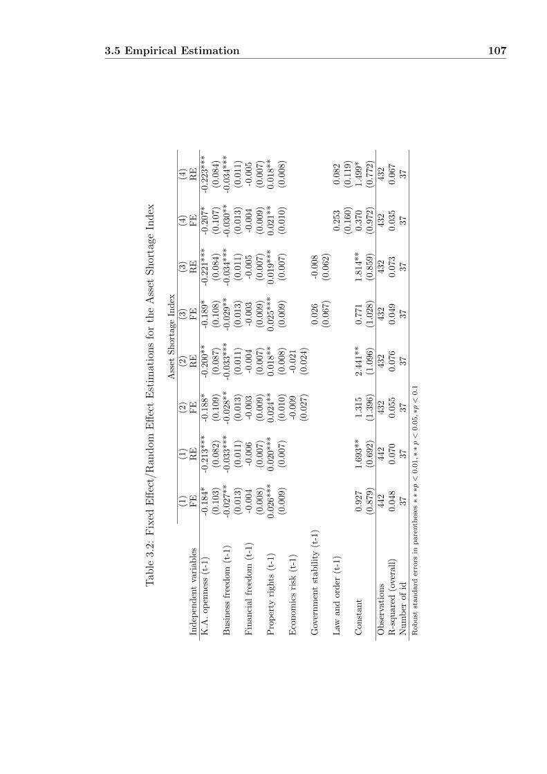
3.5 Empirical Estimation 107
Tab
le3.
2:F
ixed
Eff
ect/
Ran
dom
Eff
ect
Est
imat
ions
for
the
Ass
etShor
tage
Index
Ass
etS
hort
age
Ind
ex(1
)(1
)(2
)(2
)(3
)(3
)(4
)(4
)In
dep
end
ent
vari
able
sF
ER
EF
ER
EF
ER
EF
ER
EK
.A.
open
nes
s(t
-1)
-0.1
84*
-0.2
13***
-0.1
88*
-0.2
00**
-0.1
89*
-0.2
21***
-0.2
07*
-0.2
23***
(0.1
03)
(0.0
82)
(0.1
09)
(0.0
87)
(0.1
08)
(0.0
84)
(0.1
07)
(0.0
84)
Bu
sin
ess
free
dom
(t-1
)-0
.027
**-0
.033***
-0.0
28**
-0.0
33***
-0.0
29**
-0.0
34***
-0.0
30**
-0.0
34***
(0.0
13)
(0.0
11)
(0.0
13)
(0.0
11)
(0.0
13)
(0.0
11)
(0.0
13)
(0.0
11)
Fin
anci
alfr
eed
om(t
-1)
-0.0
04-0
.006
-0.0
03
-0.0
04
-0.0
03
-0.0
05
-0.0
04
-0.0
05
(0.0
08)
(0.0
07)
(0.0
09)
(0.0
07)
(0.0
09)
(0.0
07)
(0.0
09)
(0.0
07)
Pro
per
tyri
ghts
(t-1
)0.
026*
**0.0
20***
0.0
24**
0.0
18**
0.0
25***
0.0
19***
0.0
21**
0.0
18**
(0.0
09)
(0.0
07)
(0.0
10)
(0.0
08)
(0.0
09)
(0.0
07)
(0.0
10)
(0.0
08)
Eco
nom
ics
risk
(t-1
)-0
.009
-0.0
21
(0.0
27)
(0.0
24)
Gov
ern
men
tst
abil
ity
(t-1
)0.0
26
-0.0
08
(0.0
67)
(0.0
62)
Law
and
ord
er(t
-1)
0.2
53
0.0
82
(0.1
60)
(0.1
19)
Con
stan
t0.
927
1.6
93**
1.3
15
2.4
41**
0.7
71
1.8
14**
0.3
70
1.4
99*
(0.8
79)
(0.6
92)
(1.3
96)
(1.0
96)
(1.0
28)
(0.8
59)
(0.9
72)
(0.7
72)
Ob
serv
atio
ns
442
442
432
432
432
432
432
432
R-s
qu
ared
(ove
rall
)0.
048
0.0
70
0.0
55
0.0
76
0.0
49
0.0
73
0.0
35
0.0
67
Nu
mb
erof
id37
37
37
37
37
37
37
37
Rob
ust
stan
dard
erro
rsin
pare
nth
eses∗∗∗p<
0.0
1,∗∗p<
0.0
5,∗p<
0.1

3.5 Empirical Estimation 108
and is an index that measures the extent of restrictions on external accounts,
with a higher value reflecting more open cross-border capital transactions.
This result suggests that by widening the investment universe for domestic
institutional investors in EMs, and allowing savings to be invested overseas,
the domestic AS problem is reduced.
The business freedom index is statistically significant and negative, sug-
gesting that a friendlier business environment reduces the AS index. The
business freedom score is composed of various factors with equal weights: pro-
cedures, time, cost, and minimum capital for starting a business, obtaining a
license and the time, cost recovery rate for closing a business. The business
freedom index ranges from 0 to 100; a higher value implies a more friendly
business environment. As the business environment improves, investors will
find it easier to create new businesses and invest, thereby increasing the sup-
ply of financial assets and decreasing the asset shortage.
The financial freedom index, stronger property rights, and macroeconomic
risks (Government stability) have no significant impact on reducing the asset
shortages. The financial freedom index is a measure of government interven-
tion in the financial markets, with higher values representing fewer regulations
imposed by the government. Our finding shows that countries with stronger
government intervention in capital markets do not have larger asset shortages
than less interventionist countries. Stronger property rights are not found to
lead to greater issuance of financial assets. Intuitively, it would be expected
that stronger property rights, by increasing protection, should be good for
asset issuance. As EMs are still catching up, and therefore use existing tech-
nologies to grow, stronger property rights may in fact be bad for growth
by hindering the copying of existing technologies, and hence increasing asset
shortages. Only when countries have reached sufficiently advanced develop-
ment will property rights be good for asset issuance (Chang (2001)).
Economic risk - a measure of the overall macroeconomic environment - is
shown to have insignificant effects on the AS index. The index is a compos-
ite of GDP, growth, inflation, balanced budget, and current accounts. This
suggests that improving economic stability does not matter for our countries,
perhaps because the countries in our sample are stable enough to generate
financial assets.
3.6 Conclusion and Policy Implications 109
Law and order has a positive but insignificant impact on asset shortages.
This suggests that a stronger legal system, which protects investors more
solidly, will not lead to the issuance of more financial assets relative to na-
tional savings.
We can conclude that the ease of doing business, rather than economic
stability, matters the most in reducing asset shortages. However, macroeco-
nomic factors, as well as regulation variables, also affect asset shortages.
Remark, one caveat applies when reading these results against the predic-
tion in Chapter 2. The theory suggested in Chapter 2 predicts the business
freedom (instead of the financial freedom index) to be negatively correlated
with the asset shortage index, if it has any predictive power. The reason
been that by construction the business freedom index captures the idea of
minimum percentage of capital (as share of income per capita) required to
start-up a business, where a lower percentage represents a more friendly busi-
ness environment reflected as a higher business freedom score. Therefore,
when the asymmetric financial market arises as discussed in Chapter 2, it
translates into a higher minimum percentage of capital required to start-up
(a lower business freedom score), hence it worsen the asset shortage index.
Where as the financial market freedom index measures the degree in which
government’s control on financial market, one reason that it is insignificant
in explaining asset shortages, may due to the government’s ‘control’ became
more ‘invisible’ over time in the EMs.
3.6 Conclusion and Policy Implications
In this chapter, an index to proxy the asset shortages in EMs by capturing the
difference between the demand and supply of financial assets was constructed.
This allowed the analysis of the evolution of asset shortages over time. To
our knowledge, this is the first such measure to have been constructed. This
index provides a quantitative measure to study asset shortages. To reduce
the imbalances between supply and demand for financial assets in EMs, but
even more so to frontier markets - the subset of emerging markets with small
and illiquid market capitalizations - several policy measures could help:
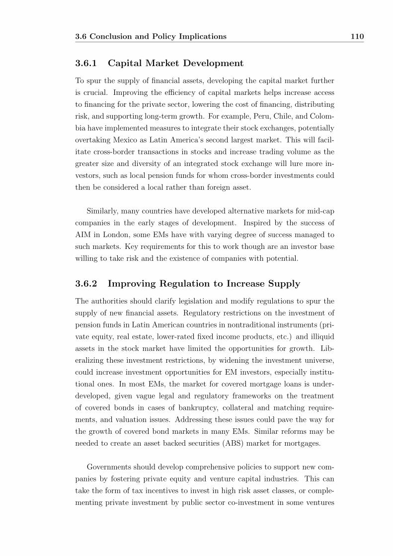
3.6 Conclusion and Policy Implications 110
3.6.1 Capital Market Development
To spur the supply of financial assets, developing the capital market further
is crucial. Improving the efficiency of capital markets helps increase access
to financing for the private sector, lowering the cost of financing, distributing
risk, and supporting long-term growth. For example, Peru, Chile, and Colom-
bia have implemented measures to integrate their stock exchanges, potentially
overtaking Mexico as Latin America’s second largest market. This will facil-
itate cross-border transactions in stocks and increase trading volume as the
greater size and diversity of an integrated stock exchange will lure more in-
vestors, such as local pension funds for whom cross-border investments could
then be considered a local rather than foreign asset.
Similarly, many countries have developed alternative markets for mid-cap
companies in the early stages of development. Inspired by the success of
AIM in London, some EMs have with varying degree of success managed to
such markets. Key requirements for this to work though are an investor base
willing to take risk and the existence of companies with potential.
3.6.2 Improving Regulation to Increase Supply
The authorities should clarify legislation and modify regulations to spur the
supply of new financial assets. Regulatory restrictions on the investment of
pension funds in Latin American countries in nontraditional instruments (pri-
vate equity, real estate, lower-rated fixed income products, etc.) and illiquid
assets in the stock market have limited the opportunities for growth. Lib-
eralizing these investment restrictions, by widening the investment universe,
could increase investment opportunities for EM investors, especially institu-
tional ones. In most EMs, the market for covered mortgage loans is under-
developed, given vague legal and regulatory frameworks on the treatment
of covered bonds in cases of bankruptcy, collateral and matching require-
ments, and valuation issues. Addressing these issues could pave the way for
the growth of covered bond markets in many EMs. Similar reforms may be
needed to create an asset backed securities (ABS) market for mortgages.
Governments should develop comprehensive policies to support new com-
panies by fostering private equity and venture capital industries. This can
take the form of tax incentives to invest in high risk asset classes, or comple-
menting private investment by public sector co-investment in some ventures

3.6 Conclusion and Policy Implications 111
targeting earlier stages of development. Brazil and South Africa are successful
examples of such policies. Asymmetric financial markets need to be removed,
policy which discriminates a certain set of firms from the credit market should
be eliminated. Moreover policymaker should take extra caution when design-
ing the policies, in order to minimizes the ‘unintended’ consequences which
create distortion in the financial markets and lead to asset shortages9.
Rules should be set in place to increase the supply of assets further by en-
forcing a minimum amount of assets that must be listed on a stock exchange.
For example, in 2010, the Ministry of Finance in India announced new rules
for companies listed on Indian bourses, requiring them to make available,
within 5 years, a minimum of 25 percent of equity, as opposed to the existing
10 percent. This should raise liquidity, and thereby reduce volatility10.
Countries with many state-owned Enterprises (SOEs) could also launch a
program to list and privatize. Malaysia is currently launching such an exer-
cise. While privatization per se is not a panacea in necessarily improving the
productivity of SOEs, it does tend to improve governance and profitability of
companies, and has the side benefit of increasing the supply of financial assets.
Regulators should remove or reduce the limit on how much institutional
investors are allowed by law to invest overseas. This would allow the system
to mitigate the excessive exposure to domestic systemic risk and the risk
of domestic security prices moving too far from fundamentals. Local market
booms tend not to persist indefinitely, and there is a need to protect retirement
savings from the swings that characterize most small and open economies.
Local markets are poorly correlated with international markets, and thus
diversification is likely to pay off in the long term. Furthermore, for crisis-
prone economies, domestic systemic risk makes it advisable to partially rely
on more stable markets. Finally, it is not necessary for the pension fund
manager to deal with foreign asset selection directly, because many reputable
international global fund managers with excellent track records can be hired
at low cost.
9See Chapter 2 for a detailed discussion.10Development of hedging instruments is also important. In this regard, the surge in the
use of derivates to hedge currency and interest rate risk bodes well for more complete capitalmarkets. Korea, Hong Kong, and Singapore have a well-developed interest rate, futures,and currency swap market, respectively, while in countries with capital account restrictions(e.g., China and India), use of the non-deliverable forward market is widespread.

3.6 Conclusion and Policy Implications 112
The business environment should be improved. Encouraging entrepreneurs
to expand by using capital markets is an important step in increasing asset
supply.
3.6.3 Reducing Savings
Too often, going public, which raises the company’s visibility, leads to regu-
latory hurdles and increased costs, thereby discouraging asset issuance. One
reason EMs have large savings rates is as a precautionary tool. Increasing
consumption can therefore also help EMs reduce asset shortages. This can be
achieved by strengthening social safety nets. High saving rates in EMs (e.g.,
China) have been described as a reflection of high individual risk, related
to costs of health, retirement, and education. Therefore it is important to
improve the ability of individuals to insure against these types of risks. For
example, in 2008 China expanded the “Yi Bao” (a Chinese state health care
system) to 229 cities.
In countries where the fiscal position is very strong and infrastructural
needs are acute, raising infrastructural investment can be a way of reducing
national savings while creating positive externalities for the rest of the econ-
omy. Following past crises, governments in EMs have been reluctant to spend
money, even if the social rate of return is very high, for fear of over-indebting
themselves. However, the positive externalities of government spending on
growth, such as infrastructure for example, could be even more important if
it leads to the supply of financial assets that could spur further development
of capital markets.
While there is no magic bullet, a comprehensive set of reforms mentioned
above will certainly help reduce the asset shortage problem, and will stim-
ulate the development of EMs further. It will improve the macroeconomic
environment of EMs, by spurring growth, leading to a better allocation of
resources, and reducing the likelihood of bubbles.

3.A Appendix 113
3.A Appendix
3.A.1 Tables
Table 3.3: Regulatory Restrictions on Pension Funds in Brazil (as of April2010, as a percentage of assets under management)
BrazilAssets Maximum LimitGovernment 100Corporate Debt 80Equities 50Real Estate Investment 8Loans and Financing 15Offshore Investment 3Corporate Debt applies for high quality assetsSource: SPC and J.P. Morgan
Table 3.4: Regulatory Restrictions on Pension Funds in Colombia (as of April2010, as a percentage of assets under management)
ColombiaAssets Maximum LimitGovernment (Domestic and External) 50Corporate Bonds 40Fogafin/Fogacoop 10Mortgage Security 40Equity/Soc. Participations 40Offshore Issued Assets (EQ+FI) 5CDs 5Source: Superfinanciera and J.P. Morgan
Table 3.5: Regulatory Restrictions on Pension Funds in Uruguay (as of April2010, as a percentage of assets under management)
UruguayAssets Maximum LimitSovereign Debt 60CB + Hipotecario Bank 30Onshore Deposits 30Hedge Operations 10Offshore Fixed Income Assets 15Source: J.P. Morgan

3.A Appendix 114
Table 3.6: Regulatory Restrictions on Pension Funds in Peru (as of April2010, as a percentage of assets under management)
PeruAssets Maximum LimitOverall Investment LimitsSovereign Debt (A) 30CB Instruments (B) 30Sovereign and CB instruments (A)+(B) 40Offshore holdings 30Maximum Limits by funds Fund 1 Fund 2 Fund 3Local and Offshore Equities 10 45 80Bonds 100 75 70Short-term Securities and Cash 40 30 30Derivatives 10 10 20Source: SBS and J.P. Morgan
Table 3.7: Regulatory Restrictions on Pension Funds in Chile (as of April2010, as a percentage of assets under management)
ChileAssets Fund A Fund B Fund C Fund D Fund EGovernment Debt 60 60 60 60 60Corporate Bonds (pri.+pub) 30 30 10 10 3Foreign Currency Investments(*) 50 40 35 25 15Equities 80 60 40 20 5CDs (Offshore) 15 15 15 15 15Mutual Funds+Invet. Funds 40 30 20 10 5Overnight Deposits 2 2 2 2 2Onshore Mutual Funds 5 5 5 5 5Net of hedge positions: an overall limit of 30 percent of AUM (unhedged) appliesfor the entire portfolio.The 15 percent limit applies to the onshore portfolio.Source: SAF JP and J.P. Morgan
Table 3.8: Regulatory Restrictions on Pension Funds in Mexico (as of April2010, as a percentage of assets under management)
MexicoAssets Fund 1 Fund 2 Fund 3 Fund 4 Fund 5Equities (domestic+Foreign 0 15 20 25 30Foreign Currency Investment 30 30 30 30 30Government Securities no limit no limit no limit no limit no limitInternational Fixed Income 20 20 20 20 20Corporate Debt no limit no limit no limit no limit no limitFinancial Institutions no limit no limit no limit no limit no limitMortgage-backed Securities no limit no limit no limit no limit no limitSemi-stat, state and Municipal entities no limit no limit no limit no limit no limitVaR (currently not published) no limit no limit no limit no limit no limitSource: Development Banks, non-bank banks, commercial banks and other financial services.

3.A Appendix 115
3.A.2 Figures
Figure 3.4: Asset Issuance by Region between 1990 and 2008 (share of GDP).Top-left: Latin America. Top-right: Eastern Europe. Bottom-left: MiddleEast and South Africa. Bottom-right: East Asia.

3.A Appendix 116
Figure 3.5: Issuance of Financial Assets in Emerging Markets between 1990and 2008 (share of GDP). Top-left: Bond. Top-right: Syndicated Loan.Bottom-left: Equity. Bottom-right: Net Purchase of Foreign Assets.

3.A Appendix 117
Figure 3.6: Bond Issuance by Region between 1990 and 2008 (share of GDP).Top-left: Latin America. Top-right: Middle East and Africa. Bottom-left:Eastern Europe. Bottom-right: East Asia.

3.A Appendix 118
Figure 3.7: Syndicated Loan Issuance by Region between 1990 and 2008(share of GDP). Top-left: Latin America. Top-right: Middle East and Africa.Bottom-left: Eastern Europe. Bottom-right: East Asia.

3.A Appendix 119
Figure 3.8: Equity Issuance by Region between 1990 and 2008 (share of GDP).Top-left: Latin America. Top-right: Middle East and Africa. Bottom-left:Eastern Europe. Bottom-right: East Asia.
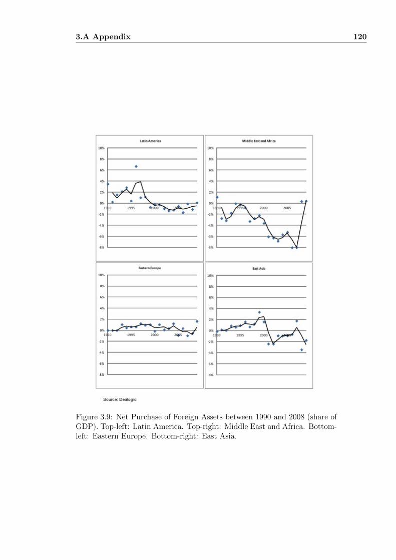
3.A Appendix 120
Figure 3.9: Net Purchase of Foreign Assets between 1990 and 2008 (share ofGDP). Top-left: Latin America. Top-right: Middle East and Africa. Bottom-left: Eastern Europe. Bottom-right: East Asia.

Chapter 4
Consequences of Asset
Shortages in Emerging Markets
4.1 Introduction
Emerging market economies (EMs) have weathered the global crisis since
2008 relatively well. Underlying the resilience were strong macroeconomic
fundamentals, the solid balance sheets of governments (low public debt), cor-
porates, and the private sector, and a tightly regulated banking system. The
rapid rebound in most EMs attests not only to the strong fundamentals, but
also to the skillful policy management of most authorities in these countries.
Yet, as illustrated in Chapter 3, despite solid fundamentals and enormous
wealth creation, EMs have not been able to generate enough financial assets
to invest their rising savings. This asset shortage is not limited to safe assets
(see Caballero (2006)) but encompasses riskier types of assets as well, rang-
ing from both fixed income to equity instruments. This is in part because
capital markets in EMs tend to be relatively shallow. They are less complex
than their counterparts in advanced economies, with banks typically playing
a larger role than non-bank financial institutions. Liquidity in these markets
is often eroded by sudden shocks, causing panic sales and disorderly adjust-
ment. In addition, the domestic investor base is not diverse enough to act as
a source of stability during a crisis. Such an underdeveloped infrastructure is
not conducive to the supply of financial assets.
This chapter proposes a theoretical model of the impact of asset shortages
on the macroeconomic environment, and after calibrating the model, also to

4.2 Theoretical Model 122
test it econometrically. This chapter aims to demonstrate that if the supply-
demand imbalance of domestically investable financial assets is not addressed,
it could potentially result in large macroeconomic imbalances that threaten
financial and macroeconomic stability. It will be shown that a shortage of
investable assets leads to suboptimal growth, as savings cannot be channeled
optimally to investment projects. In addition, asset shortages, combined with
restrictions on investment abroad, lead to excess liquidity that lowers interest
rates and raises asset prices on equity, bonds, and housing. The outcome
of too much capital chasing too few assets is bubbles followed by a crisis.
Market efficiency is also affected, as in a world of imperfect capital mobility -
owing to investment restrictions misalignments in asset valuation relative to
the economic fundamentals can be long lasting. Finally, the current account
is impacted by asset shortages, with economic agents attempting to shift their
savings overseas, creating structural surpluses.
The chapter is structured as follows. In Section II, we provide the the-
oretical model and calibrate it; in Section III, we empirically estimate the
consequences of asset shortages. Section IV concludes with policy implica-
tions.
4.2 Theoretical Model
In this section, we develop a small open economy model based on Chen (2011)
to illustrate how asset shortages in EMs lead to lower economic growth, an
increase in local asset prices, and current account surpluses. The starting
point is to divide the world into two regions: Emerging Markets (EM) and
Advanced Economies (AE), with the focus being on the former group. The
key feature of the model is that it focuses on region EM’s inability to supply
financial assets to domestic savers. The inability to generate sufficient instru-
ments locally, from safe triple A-rated store-of-value instruments to riskier
bonds and equity, increases EM savers’ demand for overseas investable in-
struments. If distortions, such as regulations, restrict the outflow, the excess
demand for investable assets will spill over into the domestic economy. EMs’
inability to create a large set of financial assets will (i) starve domestic firms
of capital, thus slowing their growth, (ii) push up domestic asset prices, and
(iii) create a current account surplus.
4.2 Theoretical Model 123
4.2.1 The Basic Structure - A Small Open Economy
The benchmark framework consists of multiple open economies, characterized
by an overlapping generation structure. This structure provides scope for
both international and intergenerational borrowings. In each region, a final
good producer manufactures one type of tradable final good (YEM ,YAE), with
each final good produced with intermediate goods that are not traded across
borders. Households own the intermediate good producing firms. In this
world, borrowing ability matters prior to production; each potential new firm
needs to make a fixed investment, which is financed by borrowing against the
present discounted value of future cash flows. The fraction of the present
value of future profits that a potential entrant can pledge is the borrowing
constraint. Furthermore, the weighted average of all agents’ borrowing ability
within each region (EM, AE) is defined as the financial development in that
region. The inability to supply financial assets is therefore akin to a tightening
of borrowing abilities.
4.2.2 Consumption
Time is evolving continuously, with infinitesimal agents born at a rate ρ per
unit time and dying at the same rate, leading to a constant population mass
equal to one. Consider an agent in region EM, who optimally decides the
consumption of the final good and savings, where he can purchase the local
assets or/and the assets issued by the intermediate firms (more on this be-
low). Following Blanchard (1985), we assume that private markets provide
insurance, and agents will contract to have all of their wealth return to the
life insurance company contingent on their death, such that agents do not
need to worry about longevity risk. If an agent’s wealth is ω, they will receive
ρω if they do not die, and pay ω if they die. By assuming agents have loga-
rithmic utility functions, optimal aggregate consumption and saving (wealth)
dynamics have the following characteristics:
Ct = (rt − τ)Ct − ρ(ρ+ τ)Wt
Wt = rtWt + At − Ct (4.1)
where, At denotes aggregate (across all household) income at time t, Wt is
the total wealth (saving) at time t, Ct is the aggregate consumption, while rt
is the exogenous foreign interest rate and τ is the (domestic) time discounting
factor.

4.2 Theoretical Model 124
The final goods produced in each region EM and AE, are traded across
borders. Therefore, the optimal intra-temporal consumption decision for an
agent in region EM or AE is:
cji,t =(P j
i,t
P jt
)−θCjt i, j = EM,AE (4.2)
where, cji,t is the consumption for final good i at time t in region j, P ji,t
is the price of good i at time t, θ is the elasticity of substitution between
goods and PEMt = PAE
t = ((1/2p1−θEM,t + 1/2p1−θ
AE,t)1
1−θ is the price index of
the consumption bundle Cjt in region EM and AE, which we normalize to
1. Since households in each region consume the same basket of final goods,
PEMt = PAE
t .
4.2.3 Production
Let us begin by focusing on the EM region. The final good producer’s pro-
duction technology uses 0 to wEM intermediate goods as inputs to produce
one unit of final good YEM :
YEM = wEM
(∫ 1
0
(yEM(i))θ−1θ di
) θθ−1
(4.3)
where, YEM denotes the final good produced in region EM, wEM refers to the
number of intermediate good producing firms in the region, and yEM(i) is the
intermediate good with i input for production. The same applies for the final
good produced in region AE.
The final good producer chooses the quantity of intermediate inputs yEM(i)
to minimize the total cost function subject to a given level of output YEM :
minyEM (i)
(wEMpEM(i)yEM(i)
)(4.4)
subject to
YEM = YEM (4.5)
gives:
y∗EM(i) =1
wEM
(PEM(i)
PEM
)−θYEM (4.6)
Intermediate good producing firms use only labor as the factor of input.
Under monopolistic competition, they set the prices at a constant mark-up
4.2 Theoretical Model 125
over the marginal costs: pEM(i) = ( θθ−1
)( vϕ(i)
), where v is the wage rate deter-
mined by labor market clearing condition1, ϕ(i) is firm i’s specific productivity
parameter. Intermediate firms take the demand as given from the final good
producer, generating a profit function at time t that has the following form:
π∗EM,t(i) =( v1−θ
θ − 1
( θ
θ − 1
)−θ)ϕθ−1EM(i)
wEM,t
(PEM,t(i)
PEM,t
)−θYEM,t (4.7)
4.2.4 Intermediate Firm Entry and Exit Decisions
• Entry.
There is a large (unbounded) pool of prospective entrants into intermedi-
ate good production. We assume that each firm is owned by an agent; initially
a firm (or agent) draws a productivity parameter ϕ from a common distribu-
tion g(ϕ). g(ϕ) has positive support over [ϕmin,∞) and has corresponding
cumulative distribution G(ϕ). To enter, each potential entrant has to make
an initial sunk investment in the form of a fixed entry cost FEM > 0. To
finance this initial fixed cost, each firm needs to borrow against its present
discounted value of future profits. Therefore, each potential entrant, given his
productivity parameter, knows the entry cost and the fraction he can borrow,
and all firms simultaneously decide whether to begin production or not.
In summary, a potential entrant will enter intermediate good production
if and only if he makes non-negative profit by entering and meets the initial
financial requirement. Consider an agent with borrowing ability δ, meaning
he can pledge δ fraction of discount value of future profits. In that case, the
entry decision rule is given by :
δEMπ∞(i)− FEM ≥ 0 (4.8)
where π∞(i) denotes the present discounted value of future profits for a po-
tential intermediate firm i.
π∞(i) =
∫ ∞t
πs(i)e−∫ st (r(τ)+ρ)dτds (4.9)
Furthermore, let Πt denote the aggregate (across all intermediate firms) profit
1We assume that labour market is operating at its natural level of employment, more-over, labour can not switch between jobs due to reasons such as skill mismatch. In contrastto Chen (2011) we make this inflexible labour market condition assumption to generate afallen output after the asset supply shock.
4.2 Theoretical Model 126
at time t.
Πt = wEM
∫ 1
0
πs(i)di (4.10)
The reservation productivity ϕ∗EM is characterized by the following equation,
implying that all potential entrants with productivity draw higher than ϕ∗EMwill enter and begin intermediate goods production.
ϕ∗EM,t =( δEMFEM
( 1
θ − 1
)1−θ ∫ ∞t
(vs)1−θω−1
EM,s(CEM,s+CAM,s)e−∫ st (r(τ)+ρ)dτds
) 11−θ
(4.11)
The Nash Equilibrium number of firms in the market is then given by:
wEM,t = 1−G(ϕ∗EM,t) (4.12)
• Exit.
Following Chen (2011) we assume, that after a firm successfully entered
the intermediate good production, it has to pay a running cost fEM,t (to its
current owner/agent) each period, which is financed by firm’s current period
profit. For example, this cost can be seem as the additional compensation to
the managers. Therefore, intermediate firm can only continues to produce if
and only if:
πEM,t(i)− fEM,t ≥ 0 (4.13)
Otherwise, firm exists the production at time t. I discuss fEM,t in more detail
in the calibration section.
4.2.5 Asset Market
One option which agents can deposit their savings is the corporate bonds
issued by intermediate firms (when they finance the initial fixed cost FEM).
The return on the corporate bond equals the dividend price ratio δEMΠEMVEM
plus the capital gain VEMVEM
. This return is equal to the world interest rate r
(which is exogenously given). At time t, this relationship is given by:
rtVEM,t = δEM,tΠEM,t + VEM,t (4.14)
Since we investigate the asset shortage problems in EMs, it is natural to focus
on a ‘small’ open economy, suggesting that the EM region takes the interest
rate as given, or put differently, the EM region is too small so it cannot affect
the world equilibrium interest rate rt.
4.2 Theoretical Model 127
Furthermore, we assume that, within each region, there exists a local asset
called L, which pays the same interest rate as the corporate bond. However,
while asset L is not traded on the international market, meaning it can only
be purchased by locals whereas corporate bonds can be purchased by both lo-
cals and foreigners. Furthermore, for reasons of riskiness, liquidity and home
bias, we assume each agent has a strict preference as to the type of asset in
which he chooses to store his savings.
Assumption 1 (Preference of Assets): Each agent has a strict preference
within different asset classes. In particular, they will firstly satisfy their needs
with domestic corporate bonds that can be traded internationally, due to
higher liquidity, followed by local asset L, because of home bias, and lastly
foreign bonds.
Moreover, due to the inability to supply assets, we assume that local asset
supply is capped at L. Finally, we introduce the definition of current account
balance in region EM:
CAEMt = WEM,t − VEM,t (4.15)
4.2.6 Calibration
Let us now calibrate the parameters for the EM region. For simplicity, we
assume standard preference parameters, with the inter-temporal elasticity of
substitution being the same for the final goods producer and household’s final
good consumption, which is fixed at θ = 2.1. The time discount factor for
the household is set at τ = 0.02 to match the average median real interest
rate in our EM country sample between 2002 and 2010. The productivity ϕ
follows a Pareto distribution, with shape parameter α equal to 2.6 and the
minimum productivity set to equal 0.2. These assumptions follow Corcos,
Gatto, Mion, and Ottaviano (2009), where they show that Pareto distribu-
tion closely fits the observed firm productivity distribution, and using a large
firm level dataset from AE, they estimate shape parameter α across different
manufacturing industries. The exogenous entry and exit rate is calibrated to
5.5 percentage points, which was calculated as the (yearly) average of the firm
entry and exit in EMs between 2002 and 2006 for a country like China (see
also Brandt, Biesebroeck, and Zhang (2009)). The initial fixed cost (FEM)
is set to equal 0.32, which is calibrated to the ratio between total fixed in-
vestments as a share of total output across EM manufacturing industries.

4.2 Theoretical Model 128
The world interest rate is assumed equal to 3 percentage points. To make
the model more manageable, we assume fEM,t(i) =πEM,t(i)
π∞(i)FEMδ
, by making
this simplification assumption the number of state variables which we need to
keep track of, is significantly reduced. Finally, since it is difficult to measure
borrowing abilities directly, we calibrate the value of ϕEM to 0.12 following
Caballero, Farhi, and Gourinchas (2006).
Given this initial calibration in region EM, we now explore a few scenarios,
which we will lay out in the parameter calibrations in the AE region.
4.2.7 Quantitative Analysis - An Asset Supply Shock
We focus on the analysis of a temporary collapse in δEM . This shock is anal-
ogous to the existence of asset shortages in region EM when investable asset
growth lags behind savings growth. This could be spurred by structural re-
forms that facilitate entrepreneurship. In order to reveal the impacts and
mechanisms of this shock, we assume that both region EM and AE start in
the same steady state prior the shock. Put differently, all the results are
driven by the shock.
Assumption 2 (Initial Conditions): The world is initially symmetric, more
specifically, δEM = δAE, implying no initial asset shortage across regions.
Suppose now, unexpectedly at t = 0, δEM drops temporally to δEM < δAE.
The fall in δEM in general could result from a structural reform or a change
in monetary policy, for instance see Chapter 3 for a detailed analysis of asset
shortages. After the shock, asset shortages appear in region EM.
Note that the definition for current account in this chapter excludes un-
expected capital gains and losses from international positions. It is not of
relevance, since at date 0, agents are assumed not to be holding international
assets. Also note that, since CAEMt +CAAEt = 0, by characterizing the CA of
EM, by default we also describe the CA of AE. Henceforth, we will focus on
describing the behavior of CAEMt , with the understanding that this concept
describes features of the global equilibrium rather than EM-specific features.
One caveat, standard models imply that capital flows from low to high
growth economies; we argue that this conclusion does not carry over to a

4.2 Theoretical Model 129
(a) Borrowing Ability in Region EM (b) Output in Region EM
(c) Asset Demand in Region EM (d) Asset Supply in Region EM
(e) Local Asset Price (f) Current Account Balance in Re-gion EM
Figure 4.1: Responses of the Key Variables After the Borrowing Ability Shock

4.3 Consequences of Asset Shortages 130
situation in which productive agents have limited ability to generate assets in
order to carry out investment. In particular, the inability to generate assets
in the EM region implies an uphill capital flow, as illustrated in empirical
work by Lucas (‘Lucas paradox’).
Figure 4.1 characterizes the path for some key variables following the col-
lapse of δEM calibrated so that Region EM’s borrowing ability falls by 25
percent (see Panel a). Panel b shows the output falls by 5 percent immedi-
ately after the shock. The reason behind this fall in output is the inability
to channel domestic savings to investment opportunities, which is reflected in
Panels c and d. When savings in the EM region rise above and beyond the
size of domestic corporate bonds, agents will increase their demand for local
assets (due to home bias), thereby driving up the price of local assets (see
Panel e). Since the local asset supply has a limit (due to the lack of asset
issuance in region EM), the excess savings is channeled to foreign investable
assets (see Panel f).
To recap, the calibration implies that an asset shortage leads to a slow-
down in economic growth, an increase in local asset prices (potentially leading
to a crisis if the asset shortage is excessive), and current account imbalances.
Having calibrated the model, we will now econometrically estimate the re-
lationship for our sample of EMs using macroeconomic data, and will con-
firm that asset shortages, as developed by in Chapter 3, constrain economic
growth, lead to domestic asset bubbles and ultimately a crisis, while also
causing current account surpluses.
4.3 Consequences of Asset Shortages
4.3.1 Economic Growth
This section will demonstrate that asset shortages owing either to insufficient
investment opportunities or to savings not being properly intermediated hold
back economic growth. In the real world, the intermediation of savings, either
via banks or capital markets, to those who have investment projects with net
present values is crucial. Without this intermediation, investment would not
get financed, leading to suboptimal growth (see also King and Levine (1993a)
and King and Levine (1993b)). It is not enough for countries to generate
savings if there is a lack of assets through which savings can be intermediated

4.3 Consequences of Asset Shortages 131
(see Chen and Imam (2011)).
Asset shortages, as measured by the asset shortage index, is therefore
likely to have an asymmetric impact on growth. Countries with asset short-
ages are likely to have credit-constrained firms, thereby holding back growth.
If there is an excess supply of financial assets, the impact on growth is likely
to be more ambiguous, because financing can also come from overseas if do-
mestic savings is insufficient and these ‘excessive’ cheap fundings can increase
investors’ risk appetite and have adverse effect on economic growth, as may
be the case in countries such as the US and UK. To test this proposition, the
AS-index is divided into two variables: (i) AS-index above zero corresponding
to a country with asset shortages at a given period of time, and (ii) AS-index
below zero representing asset surplus. We will also differentiate between the
impact of asset shortages on short-term and on long-term growth. The coun-
try classification is provided in Table 4.10. The source of data are displayed
in Table 4.11, 4.12, 4.12, 4.13, 4.14 and 4.15.
Short-Run Relationship
As many of the variables explaining asset shortages are potentially endoge-
nous, to empirically assess the impact of asset shortages on growth, we make
use of system-GMM. Another concern is robustness, as estimators are of-
ten sensitive to other conditional variables (Sala-i Martin (1997); Levine and
Renelt (1992) and Durlauf, Johnson, and Temple (2005)). Therefore, an ap-
proach suggested by Bosworth and Collins (2003) is adopted, in which the
focus is on a core set of explanatory variables that have been associated con-
sistently with growth. We then evaluate the importance of other variables
conditional on inclusion of the core set. Based on the existing literature, the
following variables are therefore included as core explanatory variables: previ-
ous economic growth, real effective exchange rate (REER), inflation and real
interest rate. Other variables such as: corruption, government deficit, world
GDP growth, GDP per capita, legal origin, US interest rate, total trade as
share of GDP, and percentage of secondary school enrollment as a proxy of
human capital are then augmented with the core regressors.
∆GDPGrowthit = β1∆ASIndex(above0)it
+ β2∆ASIndex(below0)it
+ β3∆GDPGrowthi,t−1 + β4∆REERi,t−1

4.3 Consequences of Asset Shortages 132
+ β5∆Inflationi,t−1 + β6∆Inflation2i,t−1
+ β7∆RealInterestRatei,t−1 + β8X + εit (4.16)
where X is a matrix containing all the additional variables not included
in the core regression, and β8 is the corresponding coefficient vector. Note
that the Hansen J-test and Arellano-Bond2 tests both confirm that the set of
instruments chosen for the estimation is valid, in the sense that the instru-
ments are uncorrelated with the error terms, and they satisfy the additional
restriction on the first difference.
The evidence from the econometric estimation is unambiguous. Asset
shortages negatively affect growth, while an asset surplus has no discernible
impact. The results suggest a negative relationship between change in the AS
index (truncated above zero) and subsequent GDP growth. A 1 percentage
point increase in asset shortages is associated with a slowdown in annual GDP
growth of around 0.7 percentage points, consistent with our original hypoth-
esis. This implies that, as firms become financially constrained and unable to
borrow to meet the desired level of investment, and savings are not allocated
where they are needed, growth slows down.
The findings are robust to different specifications of the regression, as
displayed in Table 4.1, with our premises mostly confirmed. In particular:
• GDP growth. If an economy has grown rapidly in the recent past, it
will revert back to a more sustainable growth rate.
• Inflation. There is evidence that inflation is statistically significant and
non-linear. While inflation has a mild positive impact on growth when
it is contained, its impact becomes negative beyond a certain threshold.
• Real interest rate. A higher real interest rate is significantly negatively
correlated with GDP growth, as high interest rates render borrowing
more expensive.
• Real exchange rate. While the real effective exchange rate is statisti-
cally significant and positive, the coefficient is close to zero. This implies
2We noticed that the Arellano-Bond test statistics are ‘too’ high in some of the regres-sion specifications, which poses potential problem - invalidity of the instruments, howeverpanel fixed effect estimations are also implemented in parallel as robustness check. Theresults are similar between two estimation procedures moreover, estimation results on othervariables are consistent with the existing literature therefore we believe the results fromGMM estimations reflect the true estimates with certain degree of consistency.

4.3 Consequences of Asset Shortages 133
Tab
le4.
1:Syst
emG
MM
Reg
ress
ion
Res
ult
sfo
rE
xpla
inin
gG
DP
Gro
wth
∆G
DP
Gro
wth
Ind
ep
en
dent
Var.
(1)
(2)
(3)
(4)
(5)
(6)
(7)
(8)
(9)
(10)
∆A
Sin
dex
-0.1
35*
(0.0
79)
∆A
Sin
dex
-0.6
95**
-0.6
95**
-0.8
75**
-0.6
83**
-0.6
96**
-0.6
92**
-0.6
70**
-0.6
92**
-0.6
73**
(tru
ncate
dab
ove
0)
(0.3
17)
(0.3
21)
(0.4
27)
(0.3
16)
(0.3
19)
(0.3
20)
(0.3
20)
(0.3
19)
(0.3
19)
∆A
Sin
dex
-0.0
16
-0.0
16
0.0
29
-0.0
01
-0.0
17
-0.0
211
-0.0
19
-0.0
18
-0.0
18
(tru
ncate
db
elo
w0)
(0.0
66)
(0.0
67)
(0.0
90)
(0.0
68)
(0.0
66)
(0.0
68)
(0.0
66)
(0.0
66)
(0.0
67)
∆G
DP
gro
wth
(t-1
)-0
.281***
-0.2
73***
-0.2
73***
-0.2
84***
-0.2
94***
-0.2
75***
-0.2
76***
-0.2
82***
-0.2
77***
-0.2
84***
(0.0
37)
(0.0
40)
(0.0
41)
(0.0
45)
(0.0
42)
(0.0
41)
(0.0
392)
(0.0
41)
(0.0
41)
(0.0
41)
∆R
EE
R0.0
01***
0.0
01***
0.0
01**
0.0
01***
0.0
01***
0.0
01***
0.0
01***
0.0
01***
0.0
01***
0.0
01***
(0.0
003)
(0.0
003)
(0.0
004)
(0.0
004)
(0.0
003)
(0.0
004)
(0.0
003)
(0.0
003)
(0.0
003)
(0.0
003)
∆In
flati
on
-0.3
94***
-0.3
86***
-0.3
86***
-0.5
06***
-0.4
08***
-0.3
88***
-0.3
89***
-0.3
92***
-0.3
90***
-0.3
94***
(0.1
06)
(0.1
06)
(0.1
08)
(0.1
23)
(0.1
08)
(0.1
08)
(0.1
07)
(0.1
08)
(0.1
07)
(0.1
07)
∆In
flati
on
squ
are
d0.0
02**
0.0
02**
0.0
02**
0.0
03***
0.0
02**
0.0
02**
0.0
02**
0.0
02**
0.0
02**
0.0
02**
(0.0
01)
(0.0
01)
(0.0
01)
(0.0
01)
(0.0
01)
(0.0
01)
(0.0
01)
(0.0
01)
(0.0
01)
(0.0
01)
∆R
eal
inte
rest
rate
-0.1
84***
-0.1
82***
-0.1
82***
-0.1
78***
-0.1
59***
-0.1
81***
-0.1
81***
-0.1
74***
-0.1
80***
-0.1
74***
(0.0
35)
(0.0
34)
(0.0
34)
(0.0
39)
(0.0
34)
(0.0
34)
(0.0
34)
(0.0
34)
(0.0
34)
(0.0
34)
∆C
orr
up
tion
-0.0
04
(0.4
26)
Govern
ment
defi
cit
0.0
15
(0.0
19)
Worl
dG
DP
gro
wth
5.8
40***
(1.8
83)
GD
Pp
er
cap
ita
0.0
00009
(0.0
0001)
Com
mon
law
0.2
62**
(0.1
15)
Secon
dary
ed
u.
0.0
05*
(perc
enta
ge)
(0.0
03)
US
inte
rest
rate
(t-1
)0.0
28
(0.0
33)
Tota
ltr
ad
e/G
DP
(t-1
)0.0
03**
(0.0
01)
Are
llan
o-B
on
dte
stfo
r0.3
88
0.4
01
0.3
98
0.3
96
0.3
83
0.3
96
0.3
93
0.3
68
0.3
60
0.3
67
AR
(2)
infi
rst
diff
Han
sen
test
of
overi
de
0.9
20.9
50.9
00.9
30.9
20.9
10.9
20.9
20.9
20.9
2re
stri
cti
on
sR
obust
standard
errors
inparentheses.∗∗∗p<
0.0
1,∗∗p<
0.0
5,∗p<
0.1
4.3 Consequences of Asset Shortages 134
that its impact on growth matters, though only in a limited way. This
could reflect the heterogeneity of our sample, which includes commod-
ity producers and manufacturing economies, which have very different
elasticities of exports and imports.
We now turn to the additional variables entered into the base regression
separately.
• Government deficit. Government deficit is positively correlated with
GDP growth, but is not statistically significant. This implies mild
evidence for the validity of the Ricardian equivalence in EMs, which
postulates that consumers internalize government’s budget constraint.
Taxpayers put aside savings to pay for expected future tax increases,
offsetting any positive impact of a budget deficit on growth.
• World GDP growth. World GDP growth, a proxy for overseas eco-
nomic conditions, has a positive and significant impact on domestic
GDP growth. Better global growth means higher exports and positive
effects on consumer and investor confidence.
• US interest rates. US interest rates, a proxy for worldwide monetary
policy, have a positive impact on domestic GDP growth. One hypothesis
would be that higher US interest rates, by making it more difficult to
borrow overseas, might encourage local investors to borrow domestically
instead, thereby stimulating growth.
• GDP per capita. GDP per capita is positively correlated with GDP
growth but is not statistically significant. While we therefore do not
see evidence of a convergence effect, this might be because all of our
countries are part of a similar income group, suggesting that they may
already have converged to similar steady states.
• Openness. More openness, by encouraging specialization in the produc-
tion of goods and services, benefits the domestic and the world economy.
• Common law. UK legal origin, a proxy for common law, has a posi-
tive and statistically significant effect on GDP growth, as confirmed in
several studies. According to this literature, common law is more cred-
itor friendly than civil law, and hence creates a more dynamic economy
(La Porta, Lopez-de Silanes, Shleifer, and Vishny (1997)).
4.3 Consequences of Asset Shortages 135
• Corruption. Change in corruption has no significant impact on GDP
growth. Corruption is not always bad for growth, if, like a tax, it is
predictable and facilitates transactions. Some studies have suggested
that in EMs, notably in East Asia, greasing the wheels of government
may have helped spur growth (Khan (2001)).
• Human capital. Human capital, as one would expect from theory, is an
important factor determining GDP growth.
Long-run Relationship
This subsection examines the long-run nature of the relationship between as-
set shortages and economic growth. Thus far, we have looked at their short-
run relationship, ignoring both whether a long-run relationship exists and
causality. We first use a panel unit root (Im, Pesaran, and Shin (2003)) and
panel co-integration tests (Pedroni (1999) and Pedroni (2004)) to determine
the long-run relationship. These allow for heterogeneity in coefficients and
different dynamics across units. This enables us to determine the long-run
structure of the asset shortage and growth relationship, avoiding the prob-
lems of low power that occur in traditional (time series) co-integration testing
owing to the small samples. We also test the direction of the causality by em-
ploying a panel co-integration causality test (Canning and Pedroni (2008)).
Before embarking on co-integration techniques, we need to test for non-
stationarity against the alternative that the variables are trend stationary,
where we allow different intercepts and time trends for each country. We
adopt the Im, Pesaran, and Shin (2003) approach, which allows each panel
member to have a different autoregressive parameter and short-run dynamics
under the alternative hypothesis of trend stationarity. The variables GDP
growth and the AS index are tested both in levels and in first difference. We
cannot reject the null hypothesis (i.e., unit root) at levels; however, the null
hypothesis is rejected at the 1 percent significance level when differences are
tested. In what follows, we therefore proceed on the assumption that all vari-
ables are I(1) and all difference variables are I(0) (Table 4.7).
As the order of stationarity has been confirmed, we next turn to the ques-
tion of possible co-integration between asset shortage and GDP growth. Given
the possibility of reverse causality between the two variables, the panel co-
integration technique of Pedroni (1999) and Pedroni (2004) is adopted. It is
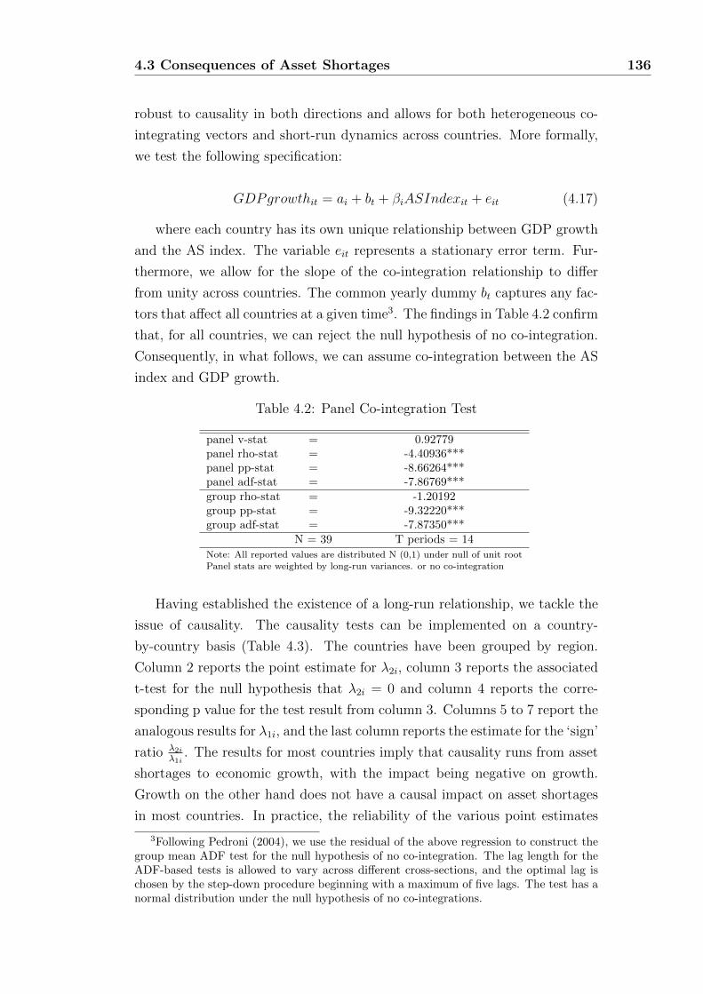
4.3 Consequences of Asset Shortages 136
robust to causality in both directions and allows for both heterogeneous co-
integrating vectors and short-run dynamics across countries. More formally,
we test the following specification:
GDPgrowthit = ai + bt + βiASIndexit + eit (4.17)
where each country has its own unique relationship between GDP growth
and the AS index. The variable eit represents a stationary error term. Fur-
thermore, we allow for the slope of the co-integration relationship to differ
from unity across countries. The common yearly dummy bt captures any fac-
tors that affect all countries at a given time3. The findings in Table 4.2 confirm
that, for all countries, we can reject the null hypothesis of no co-integration.
Consequently, in what follows, we can assume co-integration between the AS
index and GDP growth.
Table 4.2: Panel Co-integration Test
panel v-stat = 0.92779panel rho-stat = -4.40936***panel pp-stat = -8.66264***panel adf-stat = -7.86769***group rho-stat = -1.20192group pp-stat = -9.32220***group adf-stat = -7.87350***
N = 39 T periods = 14Note: All reported values are distributed N (0,1) under null of unit rootPanel stats are weighted by long-run variances. or no co-integration
Having established the existence of a long-run relationship, we tackle the
issue of causality. The causality tests can be implemented on a country-
by-country basis (Table 4.3). The countries have been grouped by region.
Column 2 reports the point estimate for λ2i, column 3 reports the associated
t-test for the null hypothesis that λ2i = 0 and column 4 reports the corre-
sponding p value for the test result from column 3. Columns 5 to 7 report the
analogous results for λ1i, and the last column reports the estimate for the ‘sign’
ratio λ2i
λ1i. The results for most countries imply that causality runs from asset
shortages to economic growth, with the impact being negative on growth.
Growth on the other hand does not have a causal impact on asset shortages
in most countries. In practice, the reliability of the various point estimates
3Following Pedroni (2004), we use the residual of the above regression to construct thegroup mean ADF test for the null hypothesis of no co-integration. The lag length for theADF-based tests is allowed to vary across different cross-sections, and the optimal lag ischosen by the step-down procedure beginning with a maximum of five lags. The test has anormal distribution under the null hypothesis of no co-integrations.
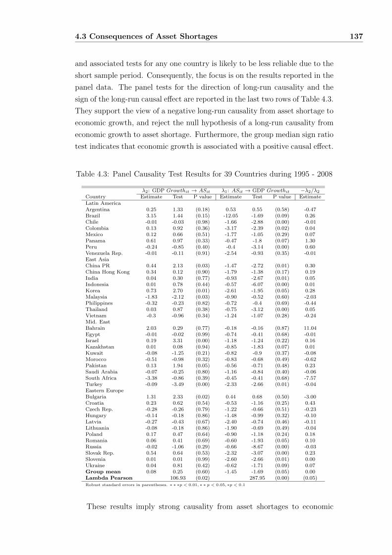
4.3 Consequences of Asset Shortages 137
and associated tests for any one country is likely to be less reliable due to the
short sample period. Consequently, the focus is on the results reported in the
panel data. The panel tests for the direction of long-run causality and the
sign of the long-run causal effect are reported in the last two rows of Table 4.3.
They support the view of a negative long-run causality from asset shortage to
economic growth, and reject the null hypothesis of a long-run causality from
economic growth to asset shortage. Furthermore, the group median sign ratio
test indicates that economic growth is associated with a positive causal effect.
Table 4.3: Panel Causality Test Results for 39 Countries during 1995 - 2008
λ2: GDP Growthit → ASit λ1: ASit → GDP Growthit −λ2/λ2
Country Estimate Test P value Estimate Test P value EstimateLatin AmericaArgentina 0.25 1.33 (0.18) 0.53 0.55 (0.58) -0.47Brazil 3.15 1.44 (0.15) -12.05 -1.69 (0.09) 0.26Chile -0.01 -0.03 (0.98) -1.66 -2.88 (0.00) -0.01Colombia 0.13 0.92 (0.36) -3.17 -2.39 (0.02) 0.04Mexico 0.12 0.66 (0.51) -1.77 -1.05 (0.29) 0.07Panama 0.61 0.97 (0.33) -0.47 -1.8 (0.07) 1.30Peru -0.24 -0.85 (0.40) -0.4 -3.14 (0.00) 0.60Venezuela Rep. -0.01 -0.11 (0.91) -2.54 -0.93 (0.35) -0.01East AsiaChina PR 0.44 2.13 (0.03) -1.47 -2.72 (0.01) 0.30China Hong Kong 0.34 0.12 (0.90) -1.79 -1.38 (0.17) 0.19India 0.04 0.30 (0.77) -0.93 -2.67 (0.01) 0.05Indonesia 0.01 0.78 (0.44) -0.57 -6.07 (0.00) 0.01Korea 0.73 2.70 (0.01) -2.61 -1.95 (0.05) 0.28Malaysia -1.83 -2.12 (0.03) -0.90 -0.52 (0.60) -2.03Philippines -0.32 -0.23 (0.82) -0.72 -0.4 (0.69) -0.44Thailand 0.03 0.87 (0.38) -0.75 -3.12 (0.00) 0.05Vietnam -0.3 -0.96 (0.34) -1.24 -1.07 (0.28) -0.24Mid. EastBahrain 2.03 0.29 (0.77) -0.18 -0.16 (0.87) 11.04Egypt -0.01 -0.02 (0.99) -0.74 -0.41 (0.68) -0.01Israel 0.19 3.31 (0.00) -1.18 -1.24 (0.22) 0.16Kazakhstan 0.01 0.08 (0.94) -0.85 -1.83 (0.07) 0.01Kuwait -0.08 -1.25 (0.21) -0.82 -0.9 (0.37) -0.08Morocco -0.51 -0.98 (0.32) -0.83 -0.68 (0.49) -0.62Pakistan 0.13 1.94 (0.05) -0.56 -0.71 (0.48) 0.23Saudi Arabia -0.07 -0.25 (0.80) -1.16 -0.84 (0.40) -0.06South Africa -3.38 -0.86 (0.39) -0.45 -0.41 (0.68) -7.57Turkey -0.09 -3.49 (0.00) -2.33 -2.66 (0.01) -0.04Eastern EuropeBulgaria 1.31 2.33 (0.02) 0.44 0.68 (0.50) -3.00Croatia 0.23 0.62 (0.54) -0.53 -1.16 (0.25) 0.43Czech Rep. -0.28 -0.26 (0.79) -1.22 -0.66 (0.51) -0.23Hungary -0.14 -0.18 (0.86) -1.48 -0.99 (0.32) -0.10Latvia -0.27 -0.43 (0.67) -2.40 -0.74 (0.46) -0.11Lithuania -0.08 -0.18 (0.86) -1.90 -0.69 (0.49) -0.04Poland 0.17 0.47 (0.64) -0.90 -1.18 (0.24) 0.18Romania 0.06 0.41 (0.69) -0.60 -1.93 (0.05) 0.10Russia -0.02 -1.06 (0.29) -0.66 -8.67 (0.00) -0.03Slovak Rep. 0.54 0.64 (0.53) -2.32 -3.07 (0.00) 0.23Slovenia 0.01 0.01 (0.99) -2.60 -2.66 (0.01) 0.00Ukraine 0.04 0.81 (0.42) -0.62 -1.71 (0.09) 0.07Group mean 0.08 0.25 (0.60) -1.45 -1.69 (0.05) 0.00Lambda Pearson 106.93 (0.02) 287.95 (0.00) (0.05)Robust standard errors in parentheses. ∗ ∗ ∗p < 0.01, ∗ ∗ p < 0.05, ∗p < 0.1
These results imply strong causality from asset shortages to economic
4.3 Consequences of Asset Shortages 138
growth. Moreover, the point estimate is negative, meaning that a higher
asset shortage leads to lower economic growth, with the finding being robust
for most countries in our sample.
4.3.2 Asset Bubbles
We argued in Chapter 3 that asset bubbles have become ever more frequent.
Empirically, however, it is difficult to test for asset bubbles ex ante. Theo-
retically, rising asset bubbles tend to be (i) caused by macroeconomic factors
(e.g., overheating), or (ii) are driven by speculation. It is crucial to identify
which one of these two reasons may lead to a crisis in EMs, as the policy im-
plication can be very different. Economists typically identify the two forces
by investigating the extent to which macroeconomic variables explain asset
prices, and the variation that cannot be explained is assumed to be driven
by speculative demand. Owing to market imperfections, and given rising evi-
dence from behavioral finance that economic agents are driven by psychology
(overconfidence, heuristic bias, framing etc.) as much as by fundamentals,
the assumption that asset prices reflect market fundamentals does not always
hold. Therefore, asset prices can deviate from market fundamentals. One
factor that to our knowledge has not been explicitly tested is the impact of
asset shortages on bubbles. As Tirole (1985) argued, it is always difficult to
identify the right set of variables as proxy for market fundamentals. At the
same time finding an appropriate measure to proxy the speculative demand
is also not an easy task, however, we expect the asset shortage index captures
the ‘speculative demand’ to certain degree.
Our analysis begins by constructing an index to proxy asset over-valuation.
The methodology is based on the bubble-o-meter used in the GFSR (2010).
The asset bubble is a weighted average of three z-scores corresponding to three
major assets for each country4. The three asset classes used to construct the
asset bubble index are (i) equity, measured by a forward-looking (shorter
horizon) 12-month price-to-earnings ratio; (ii) housing market, proxied by a
price-to-rent ratio by rescaling residential house prices by rental rates; and
(iii) local sovereign bonds, estimated by local sovereign yield. The z-score
represents the deviation of the latest observation from the model prediction
and is demeaned and normalized by its standard deviation. This provides a
natural standardization for the three asset classes.
4Other assets should also be included, for example, corporate bond; but because of datalimitations in emerging economies, they are not considered in this chapter.

4.3 Consequences of Asset Shortages 139
Figure 4.2: Asset Bubbles in EMs for Equity, Government Bonds, and Hous-ing Market (z-score) between 1990 and 2008

4.3 Consequences of Asset Shortages 140
There is some evidence in our sample of countries that prices have in-
creased gradually over time for assets, though with variation across asset
classes (Figure 4.2). The housing market in EMs followed a similar pattern
to that in AEs, with a steady rise in the deviation of house prices from fun-
damentals, even after the 2008 crisis. The equity market in EMs also has
deviated above its equilibrium in recent years, though with the volatility of-
ten associated with a crisis. The z-scores for domestic sovereign bonds show a
mean reversion process, meaning that a below-model predicted yield is always
followed by a higher-than-model predicted valuation.
The intent is to estimate whether asset shortages are a key driver of asset
bubbles in EMs. We want to test whether the AS index has a significant
impact on the deviation of asset prices as predicted by its market fundamen-
tals. Besides the AS index, we use a set of macro variables that are deemed
important in determining asset prices: domestic GDP growth, inflation, real
interest rate, government fiscal balance, real effective exchange rate (REER),
legal origin, and dependency ratio. Moreover, variables that explain the in-
ternational macroeconomic environment, namely US interest rates and world
GDP growth, are also taken into account. The core regression has the follow-
ing form:
∆BubbleIndexit = β1ASIndexit + β2GDPgrowthit + β3Inflationit
+ β4RealInterestRateit + β5X + εit (4.18)
To deal both with the possibility of reverse causality and omitted variable
bias, system-GMM is again employed. Note that we lead all variables by one
year, as we assume that asset prices are priced using expectations; hence they
are not affected by contemporaneous variables, but by expected future ones.
Before deciding whether to use level effects or first difference, we test for unit
roots, with evidence of first difference, but not level effects (Table 4.8). We
therefore use first differences in asset bubble index as the dependent variable.
The results (Table 4.4) provide evidence of a strong positive link between
asset shortages and asset bubbles. Asset bubbles increase when asset short-
ages worsen. Columns 1 - 14 show that the coefficients are positive and are
statistically significant at the 5 percent level. The results imply that asset
prices will deviate from fundamentals if there is excess demand expected in
the next period.
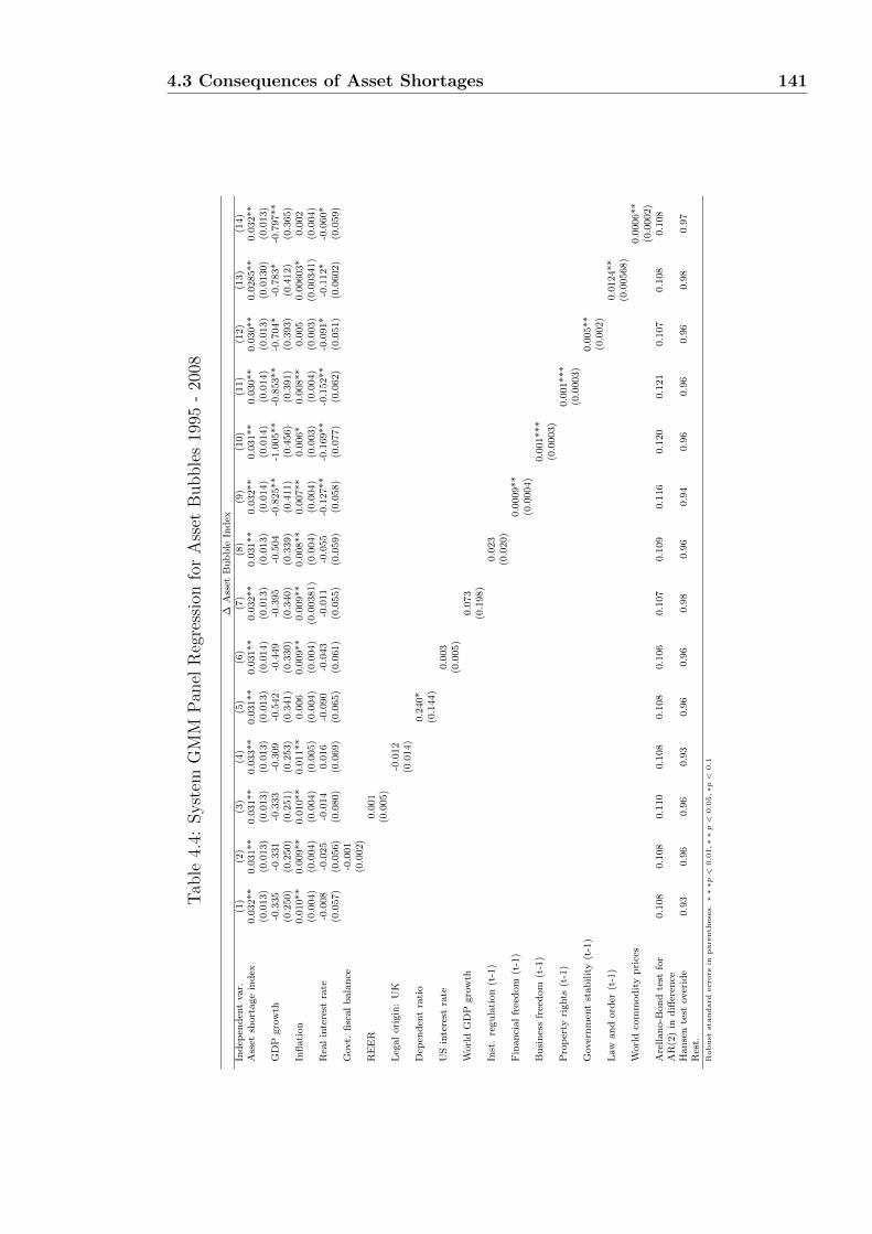
4.3 Consequences of Asset Shortages 141
Tab
le4.
4:Syst
emG
MM
Pan
elR
egre
ssio
nfo
rA
sset
Bubble
s19
95-
2008
∆A
sset
Bu
bb
leIn
dex
Ind
epen
den
tva
r.(1
)(2
)(3
)(4
)(5
)(6
)(7
)(8
)(9
)(1
0)
(11)
(12)
(13)
(14)
Ass
etsh
ort
age
ind
ex0.0
32**
0.0
31**
0.0
31**
0.0
33**
0.0
31**
0.0
31**
0.0
32**
0.0
31**
0.0
32**
0.0
31**
0.0
30**
0.0
30**
0.0
285**
0.0
32**
(0.0
13)
(0.0
13)
(0.0
13)
(0.0
13)
(0.0
13)
(0.0
14)
(0.0
13)
(0.0
13)
(0.0
14)
(0.0
14)
(0.0
14)
(0.0
13)
(0.0
130)
(0.0
13)
GD
Pgro
wth
-0.3
35
-0.3
31
-0.3
33
-0.3
09
-0.5
42
-0.4
49
-0.3
95
-0.5
04
-0.8
25**
-1.0
05**
-0.8
53**
-0.7
04*
-0.7
83*
-0.7
97**
(0.2
50)
(0.2
50)
(0.2
51)
(0.2
53)
(0.3
41)
(0.3
30)
(0.3
40)
(0.3
39)
(0.4
11)
(0.4
56)
(0.3
91)
(0.3
93)
(0.4
12)
(0.3
65)
Infl
ati
on
0.0
10**
0.0
09**
0.0
10**
0.0
11**
0.0
06
0.0
09**
0.0
09**
0.0
08**
0.0
07**
0.0
06*
0.0
08**
0.0
05
0.0
0603*
0.0
02
(0.0
04)
(0.0
04)
(0.0
04)
(0.0
05)
(0.0
04)
(0.0
04)
(0.0
0381)
(0.0
04)
(0.0
04)
(0.0
03)
(0.0
04)
(0.0
03)
(0.0
0341)
(0.0
04)
Rea
lin
tere
stra
te-0
.008
-0.0
25
-0.0
14
0.0
16
-0.0
90
-0.0
43
-0.0
11
-0.0
55
-0.1
27**
-0.1
69**
-0.1
52**
-0.0
91*
-0.1
12*
-0.0
60*
(0.0
57)
(0.0
56)
(0.0
80)
(0.0
69)
(0.0
65)
(0.0
61)
(0.0
55)
(0.0
59)
(0.0
58)
(0.0
77)
(0.0
62)
(0.0
51)
(0.0
602)
(0.0
59)
Gov
t.fi
scal
bala
nce
-0.0
01
(0.0
02)
RE
ER
0.0
01
(0.0
05)
Leg
al
ori
gin
:U
K-0
.012
(0.0
14)
Dep
end
ent
rati
o0.2
40*
(0.1
44)
US
inte
rest
rate
0.0
03
(0.0
05)
Worl
dG
DP
gro
wth
0.0
73
(0.1
98)
Inst
.re
gu
lati
on
(t-1
)0.0
23
(0.0
20)
Fin
an
cial
free
dom
(t-1
)0.0
009**
(0.0
004)
Bu
sin
ess
free
dom
(t-1
)0.0
01***
(0.0
003)
Pro
per
tyri
ghts
(t-1
)0.0
01***
(0.0
003)
Gov
ern
men
tst
ab
ilit
y(t
-1)
0.0
05**
(0.0
02)
Law
an
dord
er(t
-1)
0.0
124**
(0.0
0568)
Worl
dco
mm
od
ity
pri
ces
0.0
006**
(0.0
002)
Are
llan
o-B
on
dte
stfo
r0.1
08
0.1
08
0.1
10
0.1
08
0.1
08
0.1
06
0.1
07
0.1
09
0.1
16
0.1
20
0.1
21
0.1
07
0.1
08
0.1
08
AR
(2)
ind
iffer
ence
Han
sen
test
over
ide
0.9
30.9
60.9
60.9
30.9
60.9
60.9
80.9
60.9
40.9
60.9
60.9
60.9
80.9
7R
est.
Robust
standard
err
ors
inpare
nth
ese
s.∗∗∗p<
0.0
1,∗∗p<
0.0
5,∗p<
0.1

4.3 Consequences of Asset Shortages 142
Most fundamental factors GDP growth, interest rates, fiscal balance, real
effective exchange rate and legal origin do not have a significant impact on the
asset bubble index. This confirms that non-fundamental factors, such as psy-
chology and market imperfections, matter more in explaining bubbles. The
coefficient of GDP growth is insignificant. Similarly, real interest rates are
not statistically significant, which could be either a reflection of the limited
allocative capacity of interest rates in some EMs, or more likely the fact that
bubbles, reflecting non-fundamental factors, are unaffected by interest rate
changes, except if they are increased sharply, which rarely happens. Fiscal
balance, REER, and legal origin also are insignificant factors.
Future inflation has a positive and statistically significant impact on the
asset bubble index. This could reflect the fact that increasing inflation, a
measure associated with rising macroeconomic instability, encourages eco-
nomic actors to hedge themselves by buying assets such as equity and hous-
ing, which are either natural hedges or which have some intrinsic value.
The dependency ratio - the share of the population under 15 and over 65
over working population - has a positive impact on asset prices. In principle,
following the life-cycle hypothesis, a young population with a low dependency
ratio should lead to rising asset prices. The demographic transition, charac-
terized by an increase in the active labor force, raises demand for housing and
financial assets. Therefore, an initially falling dependency, typically leads to
rising housing and financial asset prices, creating potentially bubbles. How-
ever, Chapter 1 illustrates a significant share of the population in EMs violate
the permanent income hypothesis due to the existence of liquidity constraint.
Likewise, these liquidity constrained - unable to borrow against future in-
come - young working population will not able to raise demand for housing
and financial assets. Whereas, later on in their life time, they would either
have much higher income or accumulated a sizable stock of assets (enough to
relax the liquidity constraint) therefore start buying houses or invest in other
financial assets. As a result, Chapter 1 predicts dependent ratio should be
positively correlated with asset prices when liquidity constraint exist, which is
a common theme in EMs. Our regression results confirm that the dependency
ratio is positive and significant at 10 percent, suggesting that as a population
ages, asset prices are likely to rise, though the effect is not very strong.
World commodity prices have a positive and significant impact on the as-

4.3 Consequences of Asset Shortages 143
set bubble index. This result is not unexpected, because rising commodity
prices lead to large inflows of capital into commodity producing EMs; this
reduces the availability of financial assets for domestic investors, thereby rais-
ing prices of domestic assets. Even though rising commodity prices in general
reflect a healthy growing economy, the supply of financial assets does not ap-
pear to rise commensurately, because commodity producing countries often
finance themselves overseas or through the cash flow generated by projects,
which does not directly lead to a supply of financial assets.
US interest rates and world GDP growth, proxies for the international
macroeconomic environment, both have insignificant effects on asset bubbles
in EMs. This implies that asset bubbles are country specific phenomena, not
global. Global factors have a limited impact on EM asset prices, because
domestic regulatory and market imperfections create entry and exit barriers
in domestic asset prices (see Chen and Imam (2011)).
The regression results suggest that business friendly regulatory environ-
ments increase the probability of asset bubbles. Whether measured by busi-
ness and financial freedom, property rights, government stability, or law and
order, better regulatory environments, perhaps by providing a false sense
of security, may increase the demand for financial assets disproportionately,
thereby allowing asset bubbles to increase. Whereas the impact of institution
regulation is insignificant.
In sum, the regression estimates suggest that asset shortages have a sig-
nificant impact on asset prices. The natural question is: can asset shortages
also ‘explain’ the probability of a crisis?
4.3.3 Probability of A Crisis
Asset shortages are more likely to increase the probability of a crisis, because
too much money chasing too few financial assets leads to bubbles that if ex-
cessive can end in a crisis. Rising prices tend to create euphoria and will
attract the attention of investors. Herd behavior in turn reinforces pricing
bubbles, which eventually burst.
A probit estimation is used to study the effect of asset shortages on the
probability of crisis together with an additional set of macroeconomic vari-
4.3 Consequences of Asset Shortages 144
ables. The dependent variable (Crisis) is a binary dummy variable that takes
the value of 1 in the year crisis occurs and 0 otherwise. The regression results
are presented in Table 4.5. A set of key variables identified in the litera-
ture as major causes of crisis, including the AS index, were selected for the
econometric estimation: the log of GDP, real interest rate, a country’s credit
rating, government deficit, de facto exchange rate, inflation, and log of GDP
per capita. The analysis tests the effect of legal origin, US interest rates, ex-
ternal debt, government debt, government revenue, REER and foreign asset
liability and assets in separate regressions. Our probit regression follows:
Crisisit = β1ASIndexit + β2ln(GDP )it−1 + β3RealInterestRateit−1
+ β4Country′sCreditRatingit−1 + β5Govt.F iscalBalancei,t−1
+ β6DeFactoEx.Rate+ β7Inflationi,t−1
+ β8GDPperCapitai,t−1 + β9X + εit (4.19)
where matrix X contains a set of additional variables added to the core
regression.
The AS index has a significant and positive impact on the probability
of a crisis. The coefficient on the AS index is positive and significant across
different specifications of the regression. This means that a rise in asset short-
ages increases the probability of a crisis in the current year. Asset shortages
could be a major source of crisis, by leading to a misallocation of assets. The
imbalance between supply and demand, because it is not being addressed,
results in assets appreciating beyond their fundamentals as illustrated in the
previous section, leading to a crisis.
The coefficients of the real interest rate, income per capita, and GDP have
no statistically significant impact on the probability of crisis. As argued ear-
lier, the sensitivity of asset prices to interest rates does not seem very large,
with interest rates not leading to an equalization of demand and supply of
assets. Interest rates in EMs can increase or reduce the probability of a crisis,
depending on the credibility of monetary policy, which is high in some EMs
and low in others. The development level of an economy does not make a
crisis more likely. The size of a country’s economy and GDP per capita nei-
ther increases nor decreases the probability of a crisis, with the coefficients
being insignificant. This is not necessarily surprising, as it is not clear why
either bigger or smaller economies, or richer or poorer countries, should be
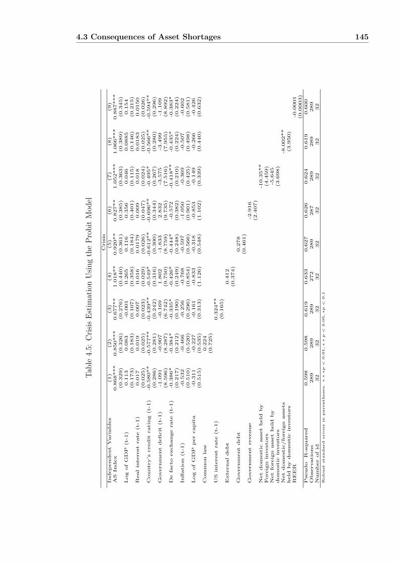
4.3 Consequences of Asset Shortages 145
Tab
le4.
5:C
risi
sE
stim
atio
nU
sing
the
Pro
bit
Model
Cris
isIn
dep
en
dent
Varia
ble
s(1)
(2)
(3)
(4)
(5)
(6)
(7)
(8)
(9)
AS
In
dex
0.8
68***
0.8
50***
0.6
77**
1.0
18**
0.9
20**
0.8
27**
1.0
52***
1.0
66***
0.8
87***
(0.3
29)
(0.3
26)
(0.2
76)
(0.4
40)
(0.3
61)
(0.3
85)
(0.3
63)
(0.3
89)
(0.3
45)
Log
of
GD
P(t-1
)0.1
13
0.0
83
-0.0
01
0.2
65
0.1
16
0.3
56
0.0
46
0.0
885
0.1
54
(0.1
73)
(0.1
83)
(0.1
07)
(0.3
58)
(0.1
84)
(0.4
01)
(0.1
15)
(0.1
46)
(0.2
15)
Real
interest
rate
(t-1
)0.0
17
0.0
19
0.0
07
0.0
16
0.0
179
0.0
09
0.0
18
0.0
183
0.0
150
(0.0
25)
(0.0
25)
(0.0
23)
(0.0
29)
(0.0
26)
(0.0
47)
(0.0
24)
(0.0
25)
(0.0
26)
Cou
ntry’s
cred
itratin
g(t-1
)-0
.580**
-0.5
77**
-0.4
39**
-0.5
49*
-0.6
12**
-0.6
96**
-0.4
95*
-0.5
66**
-0.5
94**
(0.2
86)
(0.2
81)
(0.2
42)
(0.3
16)
(0.3
00)
(0.3
44)
(0.2
67)
(0.2
80)
(0.2
96)
Govern
ment
defi
cit
(t-1
)-1
.091
-0.9
07
-0.1
69
1.8
02
-1.8
33
2.8
32
-3.5
75
-3.4
99
-1.1
09
(8.5
96)
(8.2
87)
(6.7
42)
(9.7
50)
(8.7
59)
(9.7
35)
(7.5
16)
(7.9
55)
(8.8
92)
De
facto
exch
an
ge
rate
(t-1
)-0
.386*
-0.3
84*
-0.3
35*
-0.4
26*
-0.4
44*
-0.5
72
-0.4
18**
-0.4
35*
-0.3
83*
(0.2
17)
(0.2
12)
(0.1
90)
(0.2
49)
(0.2
48)
(0.3
82)
(0.2
10)
(0.2
24)
(0.2
24)
In
flatio
n(t-1
)-0
.532
-0.4
66
-0.2
56
-0.7
68
-0.5
97
-1.0
50
-0.3
69
-0.5
07
-0.6
02
(0.5
10)
(0.5
20)
(0.2
96)
(0.8
54)
(0.5
66)
(0.9
01)
(0.4
25)
(0.4
98)
(0.5
81)
Log
of
GD
Pp
er
cap
ita
-0.3
11
-0.2
27
-0.1
61
-0.8
33
-0.3
18
-0.8
53
-0.1
49
-0.2
66
-0.4
26
(0.5
15)
(0.5
35)
(0.3
13)
(1.1
26)
(0.5
48)
(1.1
02)
(0.3
39)
(0.4
40)
(0.6
32)
Com
mon
law
0.2
24
(0.7
25)
US
interest
rate
(t-1
)0.3
24**
(0.1
65)
Extern
al
deb
t0.4
12
(0.3
74)
Govern
ment
deb
t0.2
78
(0.4
61)
Govern
ment
revenu
e-2
.916
(2.4
07)
Net
dom
estic
asset
held
by
-10.3
5**
Foreig
nin
vestors
(4.4
59)
Net
foreig
nasset
held
by
-5.6
45
dom
estic
investors
(3.6
98)
Net
dom
estic
/fo
reig
nassets
-8.0
02**
held
by
dom
estic
investors
(3.9
50)
RE
ER
-0.0
001
(0.0
003)
Pseu
do
R-s
qu
ared
0.5
98
0.5
98
0.6
19
0.6
33
0.6
27
0.6
26
0.6
24
0.6
19
0.6
00
Ob
servatio
ns
289
289
289
272
289
287
289
289
289
Nu
mb
er
of
id32
32
32
32
32
32
32
32
32
Robust
standard
errors
inparentheses.∗∗∗p<
0.01,∗∗p<
0.05,∗p<
0.1

4.3 Consequences of Asset Shortages 146
more susceptible to a crisis.
A country’s credit rating is statistically significant in explaining the prob-
ability of a crisis. The regression results suggest that, as the country’s credit
rating improves, the probability of a crisis decreases. The improvement of a
country’s credit rating is a reflection of better fundamentals in the domestic
economy, and hence better buffers against a crisis.
The probability of crisis is negatively affected by exchange rate flexibility.
In our sample, fixed change rate regimes are often observed before a crisis, for
example, the Thai baht in 1997 and the Russian ruble in 1998. Defending the
peg is difficult for any country on the eve of a crisis. Because a fixed exchange
rate is difficult to defend in the absence of a sound fiscal balance sheet and a
large accumulation of foreign reserves, it is often a source of crisis. However,
the real effective exchange rate (REER) does not have a clear impact on the
probability of a crisis. This could be because a sharp depreciation is normally
observed after a crisis, so the causality is from crisis to real exchange rate.
Key macroeconomic variables such as inflation and budget balance do not
appear to be significant in explaining the probability of a crisis. Government
fiscal balance is not statistically significant, though it does have the correct
sign. Although a budget deficit does not appear to be a key driver of crisis,
it is certainly the case that entering a crisis with a large deficit makes it more
difficult to use anti-cyclical policies. Similarly, there appears to be no close
relationship between inflation and probability of crisis. Higher inflation, by
raising instability, should lead to less confidence and lower investment levels.
Perhaps, an explanation could be that inflation over the last two decades has
been low in the EM countries we analyzed, and the evidence tends to suggest
that the negative impact of inflation on growth occurs once inflation is above
a certain threshold, typically above 20 percent or so. Common law, as proxied
by UK legal origin, is also insignificant. This suggests that legal origin is not
a major determinant of crisis.
Rising US nominal interest rates increase the probability of a crisis. The
coefficient of US nominal interest rates is positive and significant at 5 per-
cent, suggesting that rising US interest rates increase the probability of a
crisis. Rising US interest rates make domestic EM assets less attractive, lead-
ing to a reallocation of assets overseas. Capital outflow, if it accelerates, can

4.3 Consequences of Asset Shortages 147
then enhance the likelihood of a crisis.
Government debt level, external debt ratio, and government revenue have
no clear impact on the probability of a crisis. This is not surprising. Although
a government with a lower debt should, in principle, be less likely to have a
crisis, we know that government debt levels were at very different levels dur-
ing the EM crisis. The explanation could be that the debt tolerance of each
country differs, being high in some countries and low in others, which reflects
credibility arising from a country’s history of debt defaults (Reinhart, Rogoff,
and Savastano (2003)). A change in government revenue does not have a sig-
nificant impact on the probability of a crisis. This is not unexpected, because
it is revenue and expenditure jointly that matter, rather than one or the other.
The purchase of domestic financial assets a proxy for financial integration
with the world economy by foreigners increases the probability of a crisis.
In Table 4.5, the connection between net positions in foreign and domestic
assets is analyzed. The regression results show that only foreigners’ holdings
of domestic assets matter for the probability of a crisis occurring, and the
coefficients are negative and significant at the 5 percent level, while ownership
of foreign assets by domestic holders does not appear to matter in explaining
crisis. The results imply that foreign investors raise the probability of crisis,
since when they accumulate domestic assets, they effectively increase domestic
asset shortages, raising pressure for even higher asset prices.
4.3.4 Current Account
In this section, an empirical estimation of the relationship between asset short-
ages and the current account balances is undertaken. Caballero, Farhi, and
Gourinchas (2006) has argued that the current global imbalances reflect EMs’
inability to produce safe assets. Chapter 2 argued that the existence of asym-
metric financial markets can also lead to a rise in demand for asset at the
same time a fall in asset supply in EMs. In other words, EMs are unable to
generate enough assets to store their new-found wealth. On the other hand,
advanced economies notably the US and UK are able to generate such assets
easily, reflecting the strength of their capital markets. With increased liberal-
ization of capital markets, asset shortages in EMs have spillover effects, with
excess savings being channeled to overseas economies that are better able to
generate financial assets. As we argued earlier in this chapter, at the micro

4.3 Consequences of Asset Shortages 148
level, many private enterprises in EMs are credit constrained. To finance
their future investment, instead of issuing financial assets to raise funds on
capital markets, they have to raise financing through internal savings. The
rapid growth of these self-financed firms, combined with the corresponding
downsizing of banks and financial firms, creates an artificial lack of domes-
tic investment opportunities for banks. As a consequence, a growing share
of domestic savings has to be invested abroad, leading to a current account
surplus (see also Song, Storesletten, and Zilibotti (2011)).
To avoid endogeneity problems, system-GMM is again used for the esti-
mation. First difference is used, given evidence of unit roots. We test for unit
roots in the current account balance using the Im, Pesaran, and Shin (2003)
panel unit root test. Because the test suggests that the null hypothesis can-
not be rejected, the current account balance contains a unit root. The null
hypothesis in its first difference can be rejected (Table 4.9), leading to the use
of change in the current account as the dependent variable.
The starting point is to regress the change in the current account balance
on a set of core variables selected according to the literature, with additional
regulation variables added separately. Moreover, by definition, the real econ-
omy factors that drive current account balances are orthogonal to the deter-
minant of financial asset issuances; hence, by excluding the real side factors
in our regression, the results will not be biased. The following regression is
estimated:
∆CAit = β1∆CAit−1 + β2ASIndexit + β3∆Inflationit
+ β4Opennessit + β5∆RealInterestRateit
+ β6REERit + β7∆GovtF iscalBalanceit
+ β8∆WorldGDPgrowthit + β9X + εit (4.20)
The core regression includes the impact of change in the current account
lagged by one period, the AS index, openness, change in inflation and real in-
terest rate, real effective exchange rate (REER), change in government fiscal
balance, and change in world GDP growth. Subsequent regressions include
GDP per capita as a measure of the wealth of individuals, change in a coun-
try’s credit rating, overseas investment restrictions, legal origin, US interest
rate, crisis introduced as a dummy variable, exchange rate risk and term of
trade.

4.3 Consequences of Asset Shortages 149
Tab
le4.
6:E
stim
atin
gC
han
ges
inth
eC
urr
ent
Acc
ount
Usi
ng
Syst
em-G
MM
∆C
urr
ent
Accou
nt
Bala
nce
Ind
ep
en
dent.
(1)
(2)
(3)
(4)
(5)
(6)
(7)
(8)
(9)
∆C
.A.(
t-1)
-0.0
25
-0.0
37
-0.0
29
-0.0
33
-0.0
25
-0.0
43
-0.0
15
-0.0
24
-0.0
21
(0.1
07)
(0.1
24)
(0.1
11)
(0.1
14)
(0.1
07)
(0.1
06)
(0.1
08)
(0.1
06)
(0.1
05)
AS
ind
ex
0.0
07**
0.0
06**
0.0
07**
0.0
07**
0.0
07**
0.0
07**
0.0
07**
0.0
07**
0.0
07**
(0.0
03)
(0.0
03)
(0.0
03)
(0.0
04)
(0.0
03)
(0.0
04)
(0.0
03)
(0.0
04)
(0.0
03)
∆In
flati
on
0.0
13***
0.0
13***
0.0
13***
0.0
15***
0.0
14***
0.0
12***
0.0
14***
0.0
149***
0.0
16***
(0.0
02)
(0.0
02)
(0.0
02)
(0.0
02)
(0.0
02)
(0.0
02)
(0.0
02)
(0.0
02)
(0.0
02)
Op
en
ness
-0.0
0005**
-0.0
0008
-0.0
0004*
0.0
0001
-0.0
0005**
-0.0
0005**
-0.0
00001
0.0
0003
0.0
0001
(0.0
0002)
(0.0
0005)
(0.0
0002)
(0.0
0004)
(0.0
0003)
(0.0
0003)
(0.0
0003)
(0.0
0003)
(0.0
0003)
∆R
eal
0.0
01
0.0
01
0.0
01
0.0
01
0.0
0117
0.0
02
0.0
0109
0.0
01
0.0
01
inte
rest
(0.0
01)
(0.0
01)
(0.0
01)
(0.0
01)
(0.0
009)
(0.0
008)
(0.0
0101)
(0.0
01)
(0.0
01)
RE
ER
-0.0
00001***
0.0
00001***
0.0
00001***
-0.0
00001***
-0.0
00001***
-0.0
00001***
-0.0
00001***
-0.0
00001**
-0.0
00001**
(0.0
000004)
(0.0
000004)
(0.0
000004)
(0.0
000004)
(0.0
000004)
(0.0
000004)
(0.0
000004)
(0.0
000004)
(0.0
000004)
∆G
overn
ment
0.0
04*
0.0
05*
0.0
05*
0.0
05*
0.0
05*
0.0
05*
0.0
05*
0.0
05*
0.0
05*
fisc
al
bala
nce
(0.0
02)
(0.0
02)
(0.0
02)
(0.0
02)
(0.0
02)
(0.0
03)
(0.0
02)
(0.0
02)
(0.0
02)
∆W
orl
dG
DP
0.0
80*
0.0
77*
0.0
82*
0.0
84*
0.0
80*
0.0
56
0.0
695
0.0
90*
0.0
89*
gro
wth
(0.0
44)
(0.0
42)
(0.0
45)
(0.0
45)
(0.0
440)
(0.0
43)
(0.0
458)
(0.0
46)
(0.0
45)
GD
Pp
er
0.0
000004
cap
ita
(0.0
000004)
∆C
ou
ntr
ys
-0.0
09*
cre
dit
rati
ng
(0.0
05)
Regu
lati
on
-0.0
08
(0.0
05)
Com
mon
law
0.0
0237
(0.0
0356)
Cri
sis
du
mm
y(t
-1)
0.0
40***
(0.0
12)
US
inte
rest
rate
-0.0
02
(0.0
01)
Ex.
rate
risk
-0.0
01**
(0.0
004)
Term
of
trad
e-0
.0001*
(0.0
0003)
Are
llan
o-B
on
dte
st0.0
70
0.0
70
0.0
90
0.0
70
0.0
70
0.0
70
0.0
77
0.0
70
0.0
70
for
AR
(2)
infi
rst
diff
Han
sen
test
of
overi
de
0.9
80.9
90.9
60.9
60.9
60.9
60.9
60.9
60.9
6re
stri
cti
on
sR
obust
standard
errors
inparentheses.∗∗∗p<
0.0
1,∗∗p<
0.0
5,∗p<
0.1
4.3 Consequences of Asset Shortages 150
The impact of asset shortages on the current account is positive and sta-
tistically significant (see Table 4.6). This is consistent with our analysis that
EMs’ inability to generate enough financial assets relative to domestic savings
leads them to invest in overseas financial assets. The export of capital results
in a current account surplus. This finding is robust to different specifica-
tions and inclusion of different explanatory variables. The finding empirically
supports the idea advanced in Chapter 2 as well as Caballero, Farhi, and
Gourinchas (2006), though the latter’s focus mainly is on asset shortages for
safe assets, whereas our analysis argues that asset shortages in general, rather
than just safe assets, are the problem. Other key results include:
• Inflation and improvements in the fiscal balance have a positive and
statistically significant effect on the current account balance. A higher
inflation rate in the economy has a negative income effect on house-
holds, decreasing domestic consumption and reducing imports. More-
over, rising inflation tends to lead to higher uncertainty, which again
dampens investment. Similarly, improving government balances, either
via higher taxes or lower expenditure, reduces aggregate demand and
imports, thereby improving the current account.
• The real exchange rate has, as expected, a negative and statistically sig-
nificant effect on the current account balance. A depreciating currency
makes local goods more attractive in overseas markets, while render-
ing imported goods more expensive in the domestic economy, thereby
helping to improve the current account.
• A change in the real interest rate does not have a statistically significant
impact on changes in the current account. This could be a reflection of
imperfectly functioning financial markets, with the interest rate channel
not acting as an equilibrating mechanism between savings and invest-
ments. Moreover, capital flow might be driven by more than simply
interest rates.
• Our results confirm that growing world GDP improves the current ac-
count. A flourishing world economy, proxied by changes in world GDP
growth, should spur exports, thereby improving the current account.
• GDP per capita has an insignificant impact on changes in the current
account. We would have expected the coefficient to be statistically
significant, because all else being equal, poorer economies need more

4.3 Consequences of Asset Shortages 151
investment, which is likely to be financed by borrowing externally. As
capital markets are imperfect, however, this relationship may not hold.
• Capital account openness has a statistically significant and negative
relationship to changes in the current account balance. As EMs are
experiencing asset shortages, the excess savings will flow into overseas
asset markets if restrictions on investing overseas are low, but stay in
the domestic markets if these restrictions are high.
• A change in a country’s credit rating has a statistically significant and
negative impact on the current account balance. Because a credit rating
is associated with improved growth prospects and higher tolerance for
debt and shocks in general, this relationship is to be expected. As a
country moves up the rating ladder, it attracts more capital inflow from
the rest of the world, shrinking the capital account balance and thereby
raising the current account balance.
• Overseas investment restrictions (Regulation) do not have a statisti-
cal significant impact on the current account, although the sign is as
expected. The institutional restriction variable is a dummy variable,
taking the value of 1 if the restriction on institutional investors exists,
and 0 otherwise. We argue that restrictions on how institutional in-
vestors can invest overseas will reduce capital outflow and hence reduce
the current account. Perhaps, in many EMs, the institutional restriction
variable is not binding. Alternatively, our variable is too crude.
• Legal origin does not affect the current account. Legal origin is in prin-
ciple an important indicator affecting the macroeconomic environment,
as pointed out by numerous studies (e.g., La Porta, Lopez-de Silanes,
Shleifer, and Vishny (1998)). According to this literature, common law
is more creditor friendly than civil law, and hence more dynamic and
conducive to investment. We do not find such a relationship. First,
the variable might be too crude, and ignore the indirect ways through
which institutional factors could affect changes in the current account
(e.g., asset shortages, interest rates, inflation). Second, legal origin is a
variable that does not vary much over time, which can again explain its
lack of significance.
• US nominal interest rates do not have a significant negative effect on the
current account. This could reflect a lack of financial integration with

4.4 Conclusion and Policy Implications 152
the US, such that the capital flows do not respond to changes in US
interest rates. At the same time, there might be high transaction costs
or other market imperfections that make capital inflows insensitive to
US interest rates.
• Exchange rate risk has a negative impact on the current account bal-
ance. This is consistent with the finding that as exchange rate volatility
increases, risk averse investors get more cautious. Import and export
activities decline, and in extreme cases, the world ‘deglobalizes’ and the
current account closes.
• Crises, as expected, have a positive and statistically significant impact
on the current account. Crisis leads to a compression of domestic de-
mand, and hence imports.
• Terms of trade improvements have a positive impact on the current
account. An improvement in the terms of trade means a country has
to pay less per unit of imports it receives and therefore is positively
correlated with changes in the current account.
In sum, our evidence shows that asset shortages lead to current account
surpluses. One way for EMs to address the current account surpluses is to
increase the supply of financial assets, through improving economic fundamen-
tals further and improving the domestic investment environment, for instance.
4.4 Conclusion and Policy Implications
We started the chapter by modeling and calibrating the impact of asset short-
ages in EMs. The implications of the model were as follows: First, we found
that asset shortages have a negative impact on economic growth. Second,
asset shortages are a significant source of asset bubbles over time and thereby
increase the probability of a crisis. Last, asset shortages are a leading explana-
tory variable in current account surpluses of emerging markets. The macroe-
conomic implications are grave, and must be addressed to avoid macroeco-
nomic instability going forward.
Asset shortages are not only dangerous for the macroeconomic stability
of EMs, but are also a cause of the present global imbalances. Shortages of
financial assets in EMs generate permanent current account surpluses, which
are clearly not sustainable. Eventually, for creditors to repay their debt, they

4.4 Conclusion and Policy Implications 153
will either have to generate current account surpluses, or the assets owned by
EMs in AEs will have to fall in value (through exchange rate adjustment for
instance).
Given the danger that asset shortages pose for EMs and global stability
more generally, it is crucial for policy makers to tackle the problem sooner
rather than later. The arguments do not apply just to EMs, but even more
so to frontier market - the subset of emerging markets with small and illiquid
market capitalizations - because the consequences of asset shortages are par-
ticularly strong there.
Measures that would help reduce asset shortages include the following (see
Chapter 3, for other policies to address the asset shortage imbalances.):
• Correcting asymmetric financial markets. It is crucial for the policy
makers to stop favoring or discriminating a certain set of firms in access-
ing credit markets, furthermore to avoid the un-intended consequences
on financial markets when implementing policies (see Chapter 2 for a
detailed discussion).
• Deepening of domestic capital markets. It is essential that efforts be
made to deepen capital markets so as to provide a wider range of assets
for investment.
• Encouraging more domestic companies to list on the domestic stock
market and privatizing public corporations. In many EMs, tax reasons
and a judicial environment that is cumbersome and unpredictable act
as restraints on listing domestically. This would also improve financial
intermediation, thereby raising growth.
• Providing support for money to flow out. This can be achieved through
reducing the foreign investment restrictions for institutional investors.
Developing capital markets is however, a double edge sword, and may ini-
tially worsen, rather than improve the asset shortage problem. By deepening
capital markets, more capital may flow in for instance relative to the new asset
being created, while monetary policy may become less effective, and more un-
predictable. Therefore, EMs may have to live with the consequences of asset
shortages, and the resulting risk to the economy, for the foreseeable future.
Policy makers should therefore strengthen buffers to increase the resilience of
the financial system simultaneously.
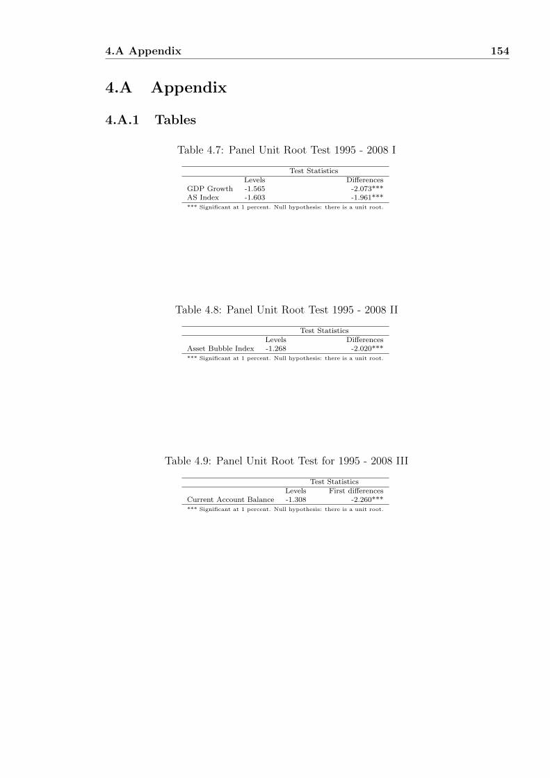
4.A Appendix 154
4.A Appendix
4.A.1 Tables
Table 4.7: Panel Unit Root Test 1995 - 2008 I
Test StatisticsLevels Differences
GDP Growth -1.565 -2.073***AS Index -1.603 -1.961****** Significant at 1 percent. Null hypothesis: there is a unit root.
Table 4.8: Panel Unit Root Test 1995 - 2008 II
Test StatisticsLevels Differences
Asset Bubble Index -1.268 -2.020****** Significant at 1 percent. Null hypothesis: there is a unit root.
Table 4.9: Panel Unit Root Test for 1995 - 2008 III
Test StatisticsLevels First differences
Current Account Balance -1.308 -2.260****** Significant at 1 percent. Null hypothesis: there is a unit root.

4.A Appendix 155
4.A.2 Data
Table 4.10: Country Classifications
Latin America East AsiaArgentina China, PRBrazil China, Hong KongChile IndiaColombia IndonesiaMexico Korea, Republic ofPanama MalaysiaPeru PhilippinesVenezuela Rep. Taiwan
ThailandVietnam
Middle East/South Africa East EuropeBahrain BulgariaEgypt CroatiaIsrael Czech RepublicKazakhstan HungaryKuwait LatviaMorocco LithuaniaPakistan PolandSaudi Arabia RomaniaSouth Africa Russia FederationTurkey Slovak RepublicUAE Slovenia
Ukraine
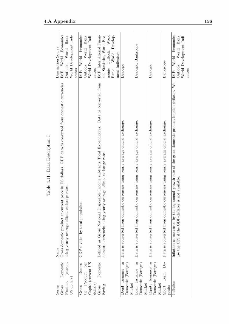
4.A Appendix 156
Tab
le4.
11:
Dat
aD
escr
ipti
onI
Ser
ies
Nam
eD
escr
ipti
on
Sou
rce
Gro
ssD
omes
tic
Pro
du
ct(c
urr
ent
US
dol
lars
)
Gro
ssd
omes
tic
pro
du
ctat
curr
ent
pri
cein
US
doll
ars
.G
DP
data
isco
nve
rted
from
dom
esti
ccu
rren
cies
usi
ng
year
lyav
erag
eoffi
cial
exch
ange
rate
s.IM
F:
Worl
dE
con
om
ics
Ou
tlook;
Worl
dB
an
k:
Worl
dD
evel
op
men
tIn
di-
cato
rsG
ross
Dom
es-
tic
Pro
du
ctp
erC
apit
a(c
urr
ent
US
dol
lars
)
GD
Pd
ivid
edby
tota
lp
opu
lati
on.
IMF
:W
orl
dE
con
om
ics
Ou
tlook;
Worl
dB
an
k:
Worl
dD
evel
op
men
tIn
di-
cato
rsG
ross
Dom
esti
cS
avin
gD
efin
edas
Gro
ssN
atio
nal
Dis
pos
able
Inco
me
sub
tract
sT
ota
lE
xp
end
itu
res.
Data
isco
nve
rted
from
dom
esti
ccu
rren
cies
usi
ng
year
lyav
erage
offi
cial
exch
an
ge
rate
s.IM
F:
Inte
rnati
on
al
Fin
an
-ci
al
Sta
tist
ics,
Worl
dE
co-
nom
icO
utl
ook;
Worl
dB
an
k:
Worl
dD
evel
op
-m
ent
Ind
icato
rsB
ond
Issu
ance
inD
omes
tic
(For
eign
)M
arke
t
Dat
ais
conve
rted
from
dom
esti
ccu
rren
cies
usi
ng
yearl
yav
erage
offi
cial
exch
an
ge.
Dea
logic
Loa
nIs
suan
cein
Dom
esti
c(F
orei
gn)
Mar
ket
Dat
ais
conve
rted
from
dom
esti
ccu
rren
cies
usi
ng
yearl
yav
erage
offi
cial
exch
an
ge.
Dea
logic
,B
an
ksc
op
e
Equ
ity
Issu
ance
inD
omes
tic
(For
eign
)M
arke
t
Dat
ais
conve
rted
from
dom
esti
ccu
rren
cies
usi
ng
yearl
yav
erage
offi
cial
exch
an
ge.
Dea
logic
Sh
ort
Ter
mD
e-p
osit
sD
ata
isco
nve
rted
from
dom
esti
ccu
rren
cies
usi
ng
yearl
yav
erage
offi
cial
exch
an
ge.
Ban
ksc
op
e
Infl
atio
nIn
flat
ion
asm
easu
red
by
the
log
annu
al
gro
wth
rate
of
the
gro
ssd
om
esti
cp
rod
uct
imp
lici
td
eflato
r.W
eu
seth
eC
PI
ifth
eG
DP
-defl
ator
isn
ot
avail
ab
le.
IMF
:W
orl
dE
con
om
ics
Ou
tlook;
Worl
dB
an
k:
Worl
dD
evel
op
men
tIn
di-
cato
rs
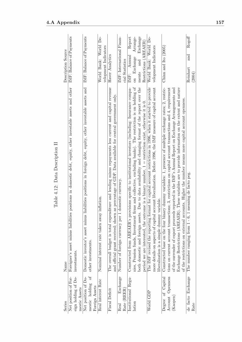
4.A Appendix 157
Tab
le4.
12:
Dat
aD
escr
ipti
onII
Ser
ies
Nam
eD
escr
ipti
on
Sou
rce
Net
pos
itio
nof
For
-ei
gnh
old
ing
ofD
o-m
esti
cA
sset
s
For
eign
er’s
asse
tm
inu
sli
abil
itie
sp
osi
tion
sin
dom
esti
cd
ebt,
equ
ity,
oth
erin
vest
ab
leass
ets
an
doth
erin
vest
men
ts.
IMF
:B
ala
nce
ofP
aym
ents
Net
pos
itio
nof
Do-
mes
tic
hol
din
gof
For
eign
Ass
ets
Dom
esti
cin
ves
tor’
sas
set
min
us
liab
ilit
ies
posi
tion
sin
fore
ign
deb
t,eq
uit
y,oth
erin
vest
ab
leass
ets
an
dot
her
inves
tmen
ts.
IMF
:B
ala
nce
ofP
aym
ents
Rea
lin
tere
stR
ate
Nom
inal
inte
rest
rate
taken
away
infl
ati
on
.W
orl
dB
an
k:
Worl
dD
e-ve
lop
men
tIn
dic
ato
rsF
isca
lD
efici
tT
he
over
all
bu
dge
tis
tota
lex
pen
dit
ure
an
dle
nd
ing
min
us
rep
aym
ents
less
curr
ent
an
dca
pit
al
reve
nu
ean
doffi
cial
gran
tre
ceiv
ed;
show
nas
per
centa
ge
of
GD
P.
Data
avail
ab
lefo
rce
ntr
al
gov
ern
men
ton
ly.
Hav
erA
naly
tics
Rea
lE
xch
ange
Rat
e(R
EE
R)
Nu
mb
erof
fore
ign
curr
ency
per
1d
om
esti
ccu
rren
cy.
IMF
:In
tern
ati
on
al
Fin
an
-ci
al
Sta
tist
ics
Inst
itu
tion
alR
egu
-la
tion
Con
stru
cted
from
AR
EA
ER
’sp
rovis
ion
ssp
ecifi
cto
inst
itu
tion
al
inve
stors
(in
clu
din
g:
Insu
ran
ceco
mp
a-
nie
s,P
ensi
onfu
nd
s,In
vest
men
tfi
rms
an
dco
llec
tive
,ex
clu
din
gb
an
ks)
.T
he
rest
rict
ion
ison
hold
ing
of
bot
hd
omes
tic
and
fore
ign
asse
ts.
Du
eto
data
avail
ab
ilit
yan
dch
an
gin
gfo
rmat
of
the
rep
ort
over
the
per
iod
we
are
inte
rest
ed,
the
outc
ome
isa
bin
ary
nu
mb
er,
1=
rest
rict
ion
exis
t,oth
erw
ise
itis
0.
IMF
:A
nnu
al
Rep
ort
on
Exch
an
ge
Arr
an
ge-
men
tsan
dE
xch
an
ge
Res
tric
tion
s(A
RE
AE
R)
Wor
ldG
DP
Th
eIM
Fre
vis
edth
ere
por
tin
gfo
rmat
for
cap
ital
acc
ou
nt
rest
rict
ion
sin
1996,
wh
enit
start
edto
pro
vid
em
ore
det
ails
onas
pec
tsof
cap
ital
acco
unt
lib
erali
zati
on
.B
efore
1996,
the
IMF
mea
sure
of
cap
italacc
ount
lib
eral
izat
ion
isa
sim
ple
du
mm
yva
riab
le.
Worl
dB
an
k:
Worl
dD
e-ve
lop
men
tIn
dic
ato
rs
Deg
ree
ofC
apit
alA
ccou
nt
Op
enn
ess
(Kao
pen
)
Con
stru
cted
bas
eon
the
fou
rb
inar
yd
um
my
vari
ab
les:
1,
pre
sen
ceof
mu
ltip
leex
chan
ge
rate
s;2,
rest
ric-
tion
son
curr
ent
acco
unt
tran
sact
ion
s;3,
rest
rict
ion
son
cap
ital
acc
ou
nt
transa
ctio
ns
an
d4,
requ
irem
ent
ofth
esu
rren
der
ofex
por
tp
roce
eds
rep
ort
edin
the
IMF
’sA
nnu
alR
eport
on
Exch
an
ge
Arr
an
gem
ents
an
dE
xch
ange
Res
tric
tion
s(A
RE
AE
R).
Th
ese
vari
ab
les
are
top
rovid
ein
form
ati
on
on
the
exte
nt
and
natu
reof
the
rest
rict
ion
son
exte
rnal
acco
unts
.H
igh
erth
enu
mb
erm
ean
sm
ore
cap
ital
acc
ou
nt
op
enn
ess.
Ch
inn
an
dIt
o(2
005)
de
fact
oE
xch
ange
Rat
eT
he
num
ber
ran
gin
gfr
om1
-6,
1m
ean
ing
de
fact
op
eg.
Rei
nh
art
and
Rogoff
(2004)

4.A Appendix 158
Tab
le4.
13:
Dat
aD
escr
ipti
onII
I
Ser
ies
Nam
eD
escr
ipti
on
Sou
rce
Inst
itu
tion
aliz
edD
emocr
acy
Dem
oc-
racy
isco
nce
ived
asth
ree
elem
ents
.1,
the
pre
sen
ceof
inst
itu
tion
san
dp
roce
du
res
thro
ugh
wh
ich
citi
zen
sca
nex
pre
sseff
ecti
vep
refe
ren
ceab
out
alte
rnati
vep
oli
cies
an
dle
ad
ers.
2,
the
exis
ten
ceof
inst
itu
tion
ali
zed
con
stra
ints
onth
eex
erci
seof
pow
erby
the
exec
uti
ve.
3,
the
gu
ara
nte
eof
civil
lib
erti
esto
all
citi
zen
sin
thei
rd
aily
live
san
din
acts
ofp
olit
ical
part
icip
ati
on
s.T
he
ind
icato
ris
an
ad
dit
ive
elev
en-p
oin
tsc
ale
(0-1
0)
Poli
cyIV
pro
ject
-U
niv
er-
sity
of
Mary
lan
d
Ed
uca
tion
Att
ain
-m
ent
(Sec
ond
ary)
Set
ofP
anel
dat
are
cord
ing
the
edu
cati
on
att
ain
men
tin
146
cou
ntr
ies
from
1950
to2010.
Barr
oan
dL
ee2010
Tra
de
Op
enn
ess
(Tot
alT
rad
e)S
um
ofim
por
tsan
dex
por
tsof
good
san
dse
rvic
esov
erG
DP
.IM
F:B
ala
nce
ofP
aym
ents
Gov
ern
men
tF
isca
lB
alan
ceIM
F:
Gov
ern
men
tF
i-n
an
ceS
tati
stic
s,S
taff
Rep
ort
;H
aver
An
aly
tics
Exte
rnal
Deb
tIM
F:
Inte
rnati
on
al
Fin
an
-ci
al
Sta
tist
ics;
Sta
ffR
e-p
ort
Gov
ern
men
tD
ebt
IMF
:G
over
nm
ent
Fi-
nan
ceS
tati
stic
s,S
taff
Rep
ort
Gov
ern
men
tR
ev-
enu
eIM
F:
Gov
ern
men
tF
i-n
an
ceS
tati
stic
s,S
taff
Rep
ort
Cou
ntr
yC
red
itR
atin
gS
hor
tte
rmC
red
itR
atin
gfo
rea
chco
untr
yw
eare
inte
rest
edov
er1990
-2009.
Fit
ch
Gov
ern
men
tS
tabil
-it
yIC
RG
pol
itic
alri
sksu
b-c
omp
onen
t(1
2p
erce
nt)
wei
ght.
Th
isis
am
easu
reb
oth
of
the
gov
ern
men
t’s
abil
ity
toca
rry
out
its
dec
lare
dp
rogr
am
(s),
an
dit
sab
ilit
yto
stay
inoffi
ce.
Th
isw
ill
dep
end
on
the
typ
eof
gove
rnan
ce,
the
coh
esio
nof
the
gover
nm
ent
an
dgov
ern
ing
part
yor
part
ies,
the
close
nes
sof
the
nex
tel
ecti
on,
the
gove
rnm
ent’
sco
mm
and
of
the
legis
latu
re,
an
dp
op
ula
rap
pro
val
of
gov
ern
men
tp
oli
cies
.
Poli
tica
lR
isk
Ser
vic
es:
In-
tern
ati
on
al
Cou
ntr
yR
isk
Gu
ide.
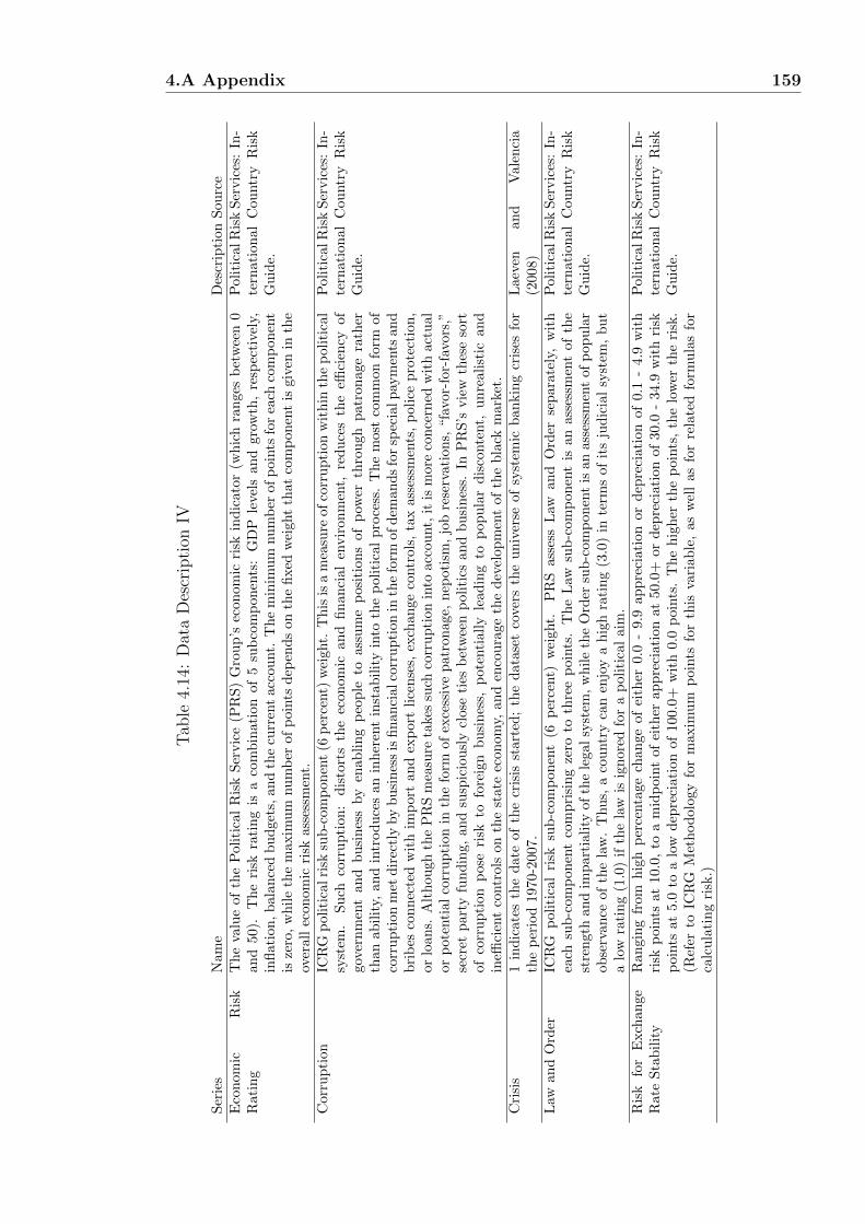
4.A Appendix 159
Tab
le4.
14:
Dat
aD
escr
ipti
onIV
Ser
ies
Nam
eD
escr
ipti
on
Sou
rce
Eco
nom
icR
isk
Rat
ing
Th
eva
lue
ofth
eP
olit
ical
Ris
kS
ervic
e(P
RS
)G
rou
p’s
econ
om
icri
skin
dic
ato
r(w
hic
hra
nges
bet
wee
n0
and
50).
Th
eri
skra
tin
gis
aco
mb
inati
on
of
5su
bco
mp
onen
ts:
GD
Ple
vels
an
dgro
wth
,re
spec
tive
ly,
infl
atio
n,b
alan
ced
bu
dge
ts,an
dth
ecu
rren
tacc
ou
nt.
Th
em
inim
um
nu
mb
erof
poin
tsfo
rea
chco
mp
on
ent
isze
ro,
wh
ile
the
max
imu
mnu
mb
erof
poin
tsd
epen
ds
on
the
fixed
wei
ght
that
com
pon
ent
isgiv
enin
the
over
all
econ
omic
risk
asse
ssm
ent.
Poli
tica
lR
isk
Ser
vic
es:
In-
tern
ati
on
al
Cou
ntr
yR
isk
Gu
ide.
Cor
rup
tion
ICR
Gp
olit
ical
risk
sub
-com
pon
ent
(6p
erce
nt)
wei
ght.
Th
isis
am
easu
reofco
rru
pti
on
wit
hin
the
politi
cal
syst
em.
Su
chco
rru
pti
on:
dis
tort
sth
eec
on
om
ican
dfi
nan
cial
envir
on
men
t,re
du
ces
the
effici
ency
of
gove
rnm
ent
and
bu
sin
ess
by
enab
lin
gp
eople
toass
um
ep
osi
tion
sof
pow
erth
rou
gh
patr
on
age
rath
erth
anab
ilit
y,an
din
trod
uce
san
inh
eren
tin
stab
ilit
yin
toth
ep
oli
tica
lp
roce
ss.
Th
em
ost
com
mon
form
of
corr
up
tion
met
dir
ectl
yby
bu
sin
ess
isfi
nan
cialco
rru
pti
on
inth
efo
rmofd
eman
ds
for
spec
ialp
aym
ents
an
db
rib
esco
nn
ecte
dw
ith
imp
ort
and
exp
ort
lice
nse
s,ex
chan
ge
contr
ols
,ta
xass
essm
ents
,p
olice
pro
tect
ion
,or
loan
s.A
lth
ough
the
PR
Sm
easu
reta
kes
such
corr
up
tion
into
acc
ou
nt,
itis
more
con
cern
edw
ith
act
ual
orp
oten
tial
corr
up
tion
inth
efo
rmof
exce
ssiv
ep
atr
on
age,
nep
oti
sm,
job
rese
rvati
on
s,“fa
vor-
for-
favo
rs,”
secr
etp
arty
fun
din
g,an
dsu
spic
iou
sly
close
ties
bet
wee
np
oli
tics
an
db
usi
nes
s.In
PR
S’s
vie
wth
ese
sort
ofco
rrup
tion
pos
eri
skto
fore
ign
bu
sin
ess,
pote
nti
all
yle
ad
ing
top
op
ula
rd
isco
nte
nt,
un
reali
stic
an
din
effici
ent
contr
ols
onth
est
ate
econ
om
y,an
den
cou
rage
the
dev
elop
men
tof
the
bla
ckm
ark
et.
Poli
tica
lR
isk
Ser
vic
es:
In-
tern
ati
on
al
Cou
ntr
yR
isk
Gu
ide.
Cri
sis
1in
dic
ates
the
dat
eof
the
cris
isst
art
ed;
the
data
set
cove
rsth
eu
niv
erse
of
syst
emic
ban
kin
gcr
ises
for
the
per
iod
1970
-200
7.L
aev
enan
dV
ale
nci
a(2
008)
Law
and
Ord
erIC
RG
pol
itic
alri
sksu
b-c
omp
onen
t(6
per
cent)
wei
ght.
PR
Sass
ess
Law
an
dO
rder
sep
ara
tely
,w
ith
each
sub
-com
pon
ent
com
pri
sin
gze
roto
thre
ep
oin
ts.
Th
eL
awsu
b-c
om
pon
ent
isan
ass
essm
ent
of
the
stre
ngt
han
dim
par
tial
ity
ofth
ele
gal
syst
em,
wh
ile
the
Ord
ersu
b-c
om
pon
ent
isan
ass
essm
ent
of
pop
ula
rob
serv
ance
ofth
ela
w.
Thu
s,a
cou
ntr
yca
nen
joy
ah
igh
rati
ng
(3.0
)in
term
sof
its
jud
icia
lsy
stem
,b
ut
alo
wra
tin
g(1
.0)
ifth
ela
wis
ign
ored
for
ap
oli
tica
laim
.
Poli
tica
lR
isk
Ser
vic
es:
In-
tern
ati
on
al
Cou
ntr
yR
isk
Gu
ide.
Ris
kfo
rE
xch
ange
Rat
eS
tab
ilit
yR
angi
ng
from
hig
hp
erce
nta
gech
ange
of
eith
er0.0
-9.
9ap
pre
ciati
on
or
dep
reci
ati
on
of
0.1
-4.
9w
ith
risk
poi
nts
at10
.0,
toa
mid
poi
nt
ofei
ther
ap
pre
ciati
on
at
50.0
+or
dep
reci
ati
on
of
30.0
-34.9
wit
hri
skp
oints
at5.0
toa
low
dep
reci
atio
nof
100.0
+w
ith
0.0
poin
ts.
Th
eh
igh
erth
ep
oin
ts,
the
low
erth
eri
sk.
(Ref
erto
ICR
GM
eth
od
olog
yfo
rm
axim
um
poin
tsfo
rth
isva
riab
le,
as
wel
las
for
rela
ted
form
ula
sfo
rca
lcu
lati
ng
risk
.)
Poli
tica
lR
isk
Ser
vic
es:
In-
tern
ati
on
al
Cou
ntr
yR
isk
Gu
ide.

4.A Appendix 160
Tab
le4.
15:
Dat
aD
escr
ipti
onV
Ser
ies
Nam
eD
escr
ipti
on
Sou
rce
Ris
kfo
rIn
flat
ion
Ran
gin
gfr
omh
igh
per
centa
geof
130+
wit
hri
skp
oin
tsat
0.0
,to
alo
wof
0.0
wit
h10.0
poin
ts.
Th
eh
igh
erth
ep
oints
,th
elo
wer
the
risk
.(R
efer
toIC
RG
Met
hod
olo
gy
for
maxim
um
poin
tsfo
rth
isva
riab
le,
asw
ell
asfo
rre
late
dfo
rmu
las
for
calc
ula
tin
gri
sk.)
Poli
tica
lR
isk
Ser
vic
es:
In-
tern
ati
on
al
Cou
ntr
yR
isk
Gu
ide.
Bu
sin
ess
Fre
edom
Bu
sin
ess
Fre
edom
isa
qu
anti
tati
vem
easu
reof
the
ab
ilit
yto
start
,op
erate
,an
dcl
ose
ab
usi
nes
sth
at
rep
rese
nts
the
over
all
bu
rden
ofre
gu
lati
on
,as
wel
las
the
effici
ency
of
gov
ern
men
tin
the
regu
lato
ryp
roce
ss.
Th
eb
usi
nes
sfr
eedom
scor
efo
rea
chco
untr
yis
anu
mb
erb
etw
een
0an
d100,
wit
h100
equ
alin
gth
efr
eest
bu
sin
ess
envir
onm
ent.
Th
eS
core
isb
ase
don
10
fact
ors
,u
sin
gd
ata
from
the
Worl
dB
an
k’s
Doi
ng
Bu
sin
ess
stu
dy.
Th
eH
erit
age
Fou
nd
ati
on
Fin
anci
alF
reed
omF
inan
cial
free
dom
isa
mea
sure
ofb
ankin
gse
curi
tyas
wel
las
am
easu
reof
ind
epen
den
cefr
om
gov
ern
men
tco
ntr
ol.
Sta
teow
ner
ship
ofb
anks
an
doth
erfi
nan
cial
inst
itu
tion
sis
an
ineffi
cien
tb
urd
enth
at
redu
ces
com
pet
itio
nan
dge
ner
ally
low
ers
the
leve
lof
avail
ab
lese
rvic
es.
Ith
as
scale
bet
wee
n0
to100,
100
mea
ns
neg
ligi
ble
gover
nm
ent
infl
uen
ce.
Th
eH
erit
age
Fou
nd
ati
on
Pro
per
tyR
ights
Pro
per
tyri
ghts
com
pon
ent
isan
asse
ssm
ent
of
the
ab
ilit
yof
ind
ivid
uals
toacc
um
ula
tep
riva
tep
rop
erty
,se
cure
dby
clea
rla
ws
that
are
full
yen
forc
edby
the
state
.It
mea
sure
sth
ed
egre
eto
wh
ich
aco
untr
y’s
law
pro
tect
pri
vate
pro
per
tyri
ghts
an
dth
ed
egre
eto
wh
ich
its
gov
ern
men
ten
forc
esth
ose
law
s.It
als
oas
sess
esth
eli
keli
hood
that
pri
vate
pro
per
tyw
ill
be
exp
rop
riate
dan
dan
aly
zes
the
ind
epen
den
ceof
the
jud
icia
ry,
the
exis
ten
ceof
corr
up
tion
wit
hin
the
jud
icia
ry,
an
dth
eab
ilit
yof
ind
ivid
uals
an
db
usi
nes
ses
toen
forc
eco
ntr
acts
.It
has
scal
eb
etw
een
0an
d100,
100
mea
ns
Pri
vate
pro
per
tyis
guara
nte
edby
the
gove
rnm
ent.
Th
eH
erit
age
Fou
nd
ati
on
Loca
lS
over
eign
Yie
ldH
aver
An
aly
tics
Exte
rnal
Sov
erei
gnC
red
itE
MB
ICS
pre
ad
Pri
ceto
Ren
tR
atio
Glo
bal
Pro
per
tyIn
dic
ato
rP
rice
and
Ear
nin
gR
atio
Blo
om
ber
g;
IBE
S
Com
mod
ity
Pri
ces
Ind
exT
he
ind
exis
con
stru
cted
usi
ng
ase
tof
wei
ghte
dco
mm
od
ity
pri
ces,
ran
gin
gfr
om
Pet
role
um
,N
atu
ral
gas;
Cop
per
,A
lum
inu
mto
Food
pri
ces.
IMF
Com
mod
ity
Ind
ex
Bibliography
Allen, F., J. Qian, and M. Qian (2008). China’s Great Economic Transforma-
tion (Loren Brandt and Thomas Rawski ed.)., Chapter China’s Financial
System: Past, Present and Future, pp. 569 – 632. Cambridge University
Press.
Altonji, J. G. and A. Siow (1987, May). Testing the response of consumption
to income changes with (noisy) panel data. Quarterly Journal of Eco-
nomics 102, 293 – 328.
Alvarez, J. and M. Arellano (2003). The time series and cross-section asymp-
totic of dynamic panel data estimators. Econometrica 71 (4), 1121 – 1159.
Amaral, P. S. and E. Quintin (2010). Limited enforcement, financial interme-
diation and economic development: A quantitative analysis. International
Economic Review 51 (3), 785 – 811.
Arellano, M. and O. Bover (1995). Another look at the instrumental variables
estimation of error-component models. Journal of Econometrics 68, 29 –
51.
Attanasio, O. P. and G. Weber (1993, July). Consumption growth, the interest
rate and aggregation. Review of Economic Studies 60, 631 – 49.
Attanasio, O. P. and G. Weber (1995). Is consumption growth consistent
with intertemporal optimization? evidence from the consumer expenditure
survey. Journal of Political Economy 103 (6), 1121 – 57.
Bacchetta, P. and K. Benhima (2010). The demand for liquid assets, corporate
saving, and global imbalance. mimeo.
Batra, G., D. Kaufmann, and A. H. Stone (2003). Investment climate around
the world: Voices of firms from the world business environment survey.
Washington, DC: World Bank .

BIBLIOGRAPHY 162
Bayoumi, T., H. Tong, and S.-J. Wei (2010). The chinese corporate sav-
ings puzzles: A firm-level cross-country perspective. NBER Working Pa-
pers (16432).
Bewley, T. (1977, December). The permanent income hypothesis: A theoret-
ical formulation. Journal of Economic Theory 16 (2), 252 – 292.
Blanchard, O. J. (1985). Debt, deficits, and finite horizons. Journal of Political
Economy 93 (2), 223 – 47.
Blundell, R. and S. Bond (1998). Initial conditions and moment restrictions
in dynamic panel data models. Journal of Econometrics 87 (7), 115 – 143.
Blundell, R., M. Browning, and C. Meghir (1994, January). Consumer de-
mand and the life-cycle allocation of household expenditures. Review of
Economic Studies 61 (1), 57 – 80.
Borensztein, E., K. Cowan, B. Eichengreen, and U. Panizza (2008). Bond
Markets in Latin America: On the Verge of a Big Bang? Cambridge MA,
The MIT Press.
Bosworth, B. and S. M. Collins (2003). The empirics of growth: An update.
Brookings papers on Economic Activity 2, 113 – 206.
Boyreau-Debray, G. and S.-J. Wei (2005). Pitfalls of a state-dominated finan-
cial system: The case of china. NBER Working Paper Series (11214).
Brandt, L., J. V. Biesebroeck, and Y. Zhang (2009). Creative accounting or
creative destruction? firm-level productivity growth in chinese manufactur-
ing. NBER Working Paper Series (15152).
Brandt, L., C.-T. Hsieh, and X. Zhu (2008). China’s Great Economic Trans-
formation (Loren Brandt and Thomas Rawski ed.)., Chapter Growth and
Structural Transformation in China. Number 569 – 632. Cambridge Uni-
versity Press.
Brandt, L. and X. Zhu (2010). Account for china’s growth. IZA Discussion
Papers (4764).
Buera, F. J., J. Kaboski, and Y. Shin (2009). Finance and development: A
tale of two sectors. NBER Working Paper Series (14914).
Buera, F. J. and Y. Shin (2010). Productivity growth and capital flows: The
dynamics of reforms. NBER Working Paper Series (15268).

BIBLIOGRAPHY 163
Caballero, R. (2006). On the macroeconomics of asset shortages. MIT Mimeo.
Caballero, R., E. Farhi, and P.-O. Gourinchas (2008). An equilibrium model
of “global imbalances” and low interest rates. American Economic Re-
view 98 (1), 358 – 393.
Caballero, R. J., E. Farhi, and P.-O. Gourinchas (2006). An equilibrium
model of “global imbalances” and low interest rate. NBER Working Paper
Series (11996).
Campbell, J. Y. and A. S. Deaton (1989, Nov). Is consumption too smooth?
NBER Working Papers (2134).
Canning, D. and P. Pedroni (2008, Sept). Infrastructure, long-run eco-
nomic growth and causality tests for cointegrated panels. The Manchester
School 76 (5), 504 – 527.
Carroll, C. and S. H. Lawrence (1989). Consumption growth parallels income
growth: Some new evidence. NBER Working Papers (3090).
Chang, H.-J. (2001). Intellectual property rights and economic development:
Historical lessons and emerging issues. Journal of Human Development and
Capabilities 2, 287 – 309.
Chen, J. (2011). Firm Productivity and the Current Account: One Country
with Two Financial Markets. Ph. D. thesis, LSE.
Chen, J. and P. Imam (2011). Causes of asset shortages in emerging markets.
IMF Working Paper (WP11/114).
Chen, J. and G. Vera (2012). What does monitors monitor?
Chinn, M. and H. Ito (2008). A new measure of financial openness. Journal
of Comparative Policy Analysis 10 (3), 309 – 322.
Coeurdacier, N., S. Guibaud, and K. Jin (2011). Credit constraints and
growth in a global economy. mimeo LSE .
Corcos, G., M. D. Gatto, G. Mion, and G. I. Ottaviano (2009). Productivity
and firm selection: Quantifying the ‘new’ gains from trade. FEEM Working
Papers (379).
de la Torre, A. and S. Schmukler (2006). Emerging Capital Markets and
Globalization: The Latin American Experience. Stanford, CA: Stanford
University Press.

BIBLIOGRAPHY 164
Deaton, A. S. (1992). Understanding Consumption. Oxford University Press.
Dollar, D. and S.-J. Wei (2007). Das(wasted) kapital: Firm ownership and
investment efficiency in china. NBER Working Paper Series (13103).
Dooley, M., D. Folkerts-Landau, and P. Garber (2003). An essay on the
revived bretton woods system. NBER Working Paper (9971).
Dooley, M. and P. Garber (2005). Is it 1958 or 1968? three notes on the
longevity of the revived bretton woods system. Brookings Papers on Eco-
nomic Activity (36), 147 – 210.
Durlauf, S., P. Johnson, and J. Temple (2005). Handbook of Economic Growth
(Philippe Aghion and Steven Durlauf ed.), Volume 1, Chapter Growth
Econometrics, pp. 555 – 677. Elsevier.
Dynan, K. E. (2000, June). Habit formation in consumer preferences: Evi-
dence from panel data. American Economic Review 90, 391 – 406.
Eichengreen, B. and R. Hausmann (1999). Exchange rates and financial
fragility. NBER Working Papers (7418).
Flavin, A. (1989). The adjustment of consumption to changing expectations
about future income. Journal of Political Economy 89, 974 – 1009.
GFSR (2010). Resolving the crisis legacy and meeting new challenges to
financial stability. GFSR.
GFSR (2012). Development of corporate bond markets in emerging market
countries. GFSR.
Greenwood, J., J. Sanchez, and C. Wang (2010). Quantifying the impact
of financial development on economic development. NBER Working Pa-
per (15893).
Hall, R. E. (1978, December). Stochastic implications of the life cycle-
permanent income hypothesis: Theory and evidence. Journal of Political
Economy 6 (6), 971 – 87.
Hall, R. E. and F. S. Mishkin (1982, March). The sensitivity of consumption
to transitory income: Estimates from panel data on households. Econo-
metrica 50 (2), 461 – 81.

BIBLIOGRAPHY 165
Hansen, L. P. and K. J. Singleton (1983, April). Stochastic consumption, risk
aversion and the temporal behavior of asset returns. Journal of Political
Economy 91, 249 – 65.
Hausmann, R. and U. Panizza (2010). Redemption or abstinence? original sin,
currency mismatches and counter-cyclical policies in the new millennium.
Center for International Development at Harvard University, Working Pa-
per (194).
Hayashi, F. (1985, November). The permanent income hypothesis and con-
sumption durability: Analysis based on japanese panel data. Quarterly
Journal of Economics. 100 (4), 1083 – 1113.
Heckman, J. J. (1974, March). Life cycle consumption and labor supply: An
explanation of the relationship between income and consumption over the
life cycle. American Economic Review. 64 (1), 188 – 94.
Hopenhayn, H. (1992). Entry, exit, and firm dynamics in long run equilibrium.
Econometrica 60, 1127 – 1150.
Hsieh, C.-T. and P. J. Klenow (2009). Misallocation and manufacturing tfp
in china and india. Quarterly Journal of Economics 124 (4), 1403 – 48.
Huang, Y. (2003). Selling China: Foreign Investment during the Reform Era.
Cambridge University Press.
Im, K. S., H. Pesaran, and Y. Shin (2003). Testing for unit roots in hetero-
geneous panels. Journals of Econometrics 115 (1), 53 – 74.
Islam, N., E. Dai, and H. Sakamoto (2006). Role of tfp in china’s growth.
Asian Economic Journal 20 (2), 127 – 59.
James, R., J. Jin, and J. Gao (2007). How China Grows: Investment, Finance
and Reform. Princeton and Oxford: Princeton University Press.
Jeong, H. and R. M. Twonsend (2005). Sources of tfp growth: Occupational
choice and financial deepening. Economic Theory 32 (1), 179 – 221.
Khan, M. (2001). The New Political Economy of Corruption (Fine, Ben,
Costas Lapavitsas and Jonathan Pincus ed.)., Chapter 6, pp. 112 – 35.
London: Routledge.
King, R. G. and R. Levine (1993a). Finance and growth: Schumpeter might
be right. Quarterly Journal of Economics 108 (3), 717 – 737.

BIBLIOGRAPHY 166
King, R. G. and R. Levine (1993b). Finance, entrepreneurship and growth.
Journal of Monetary Economics 32 (3), 513 – 542.
La Porta, R., F. Lopez-de Silanes, A. Shleifer, and R. W. Vishny (1997).
Legal determinants of external finance. Journal of Finance 52 (3), 1131 –
50.
La Porta, R., F. Lopez-de Silanes, A. Shleifer, and R. W. Vishny (1998). Law
and finance. Journal of Political Economy 106 (6), 1135 – 55.
Laeven, L. and F. Valencia (2008). Systemic banking crisis: A new database.
IMF Working Paper (WP/08/224).
Levine, R. and D. Renelt (1992). A sensitivity analysis of cross-country growth
regressions. American Economic Review 82, 942 – 63.
Ljungqvist, L. and T. J. Sargent (2004). Recursive Macroeconomic Theory
(2nd ed.). The MIT Press.
Mankiw, G. N. (1981). The permanent income hypothesis and the real interest
rate. Economics Letters 7 (4), 307 – 311.
Mankiw, N., J. J. Rotemberg, and L. H. Summers (1985, February). In-
tertemporal substitution in macroeconomics. Quarterly Journal of Eco-
nomics 100 (1), 225 – 51.
Mariger, R. P. and K. Shaw (1988). Reexamining the sensitivity of consump-
tion to transitory income. mimeo.
Matsuyama, K. (2007). Credit traps and credit cycles. American Economic
Review 97 (1), 503 – 516.
Melitz, M. (2003). The impact of trade on intra-industry reallocations and
aggregate industry productivity. Econometrica 71 (6), 1695 – 1725.
Mendoza, E. G., V. Quadrini, and J.-V. Rios-Rull (2009). Financial inte-
gration, financial development and global imbalances. Journal of Political
Economy 117 (3).
Midrigan, V. and Y. D. Xu (2010). Finance and mis-allocation evidence from
plant-level data. NBER working Paper Series (15647).
Modigliani, F. and S. L. Cao (2004, March). The chinese saving puzzle and the
life-cycle hypothesis. Journal of Economic Literature 42 (1), 145 – 170(26).
BIBLIOGRAPHY 167
Moll, B. (2010). Productivity losses from financial friction: Can self-financing
undo capital misallocation. Princeton University manuscript .
Muellbauer, J. (1988, Janvier-Mars). Habits, rationality and myopia in the
life cycle consumption function. Annales d’Economie et de Statistique (9),
04.
Neil, G. and S. Tenev (2001, March). The financing of private enterprise in
china. Finance and Development 38 (1).
Pedroni, P. (1999). Critical values for co-integration test in heterogeneous
panels with multiple regressors. Oxford Bulletin of Economics and Statis-
tics 61, 653 – 670.
Pedroni, P. (2004). Panel co-integration; asymptotic and finite sample prop-
erties of pooled time series tests, with an application to the ppp hypothesis.
Econometric Theory 20, 597 – 625.
Pesaran, H. H. and Y. Shin (1998, 1). Generalized impulse response analysis
in linear multivariate models. Economics Letters 58, 17 – 29.
Rajan, R. (2006). Investment restraint, the liquidity glut, and global imbal-
ances. http://www.imf.org/external/np/speeches/2006/111506.htm.
Reinhart, C. M., K. S. Rogoff, and M. A. Savastano (2003). Debt intolerance.
NEBR Working Paper (9908).
Runkle, D. E. (1991, February). Liquidity constraints and the permanent-
income hypothesis : Evidence from panel data. Journal of Monetary Eco-
nomics 27 (1), 73 – 98.
Sala-i Martin, X. (1997, May). I just ran two million regressions. American
Economic Review Papers and Proceedings , 178 – 183.
Sandri, D. (2010). Growth and capital flows and risky entrepreneurship. IMF
Working Paper (10/37).
Scheinkman, J. A. and L. Weiss (1986, January). Borrowing constraints and
aggregate economic activity. Econometrica 54 (1), 23 – 45.
Shih, V. (2004). Factions matter: Personal networks and the distribution of
bank loans in china. Journal of Contemporary China 13:38, 3 – 19.
Song, Z., K. Storesletten, and F. Zilibotti (2011). Growing like china. Amer-
ican Economics Review 101, 202 – 241.
BIBLIOGRAPHY 168
Sufi, A. (2007, April). Information asymmetry and financing arrangements:
Evidence from syndicated loans. Journal of Finance 62 (2).
Tirole, J. (1985). Asset bubbles and overlapping generations. Economet-
rica 53, 1499 – 1528.
Zeldes, S. P. (1987). The effects of borrowing constraints on consumption in
a multiperiod model with income uncertainty. Manuscript. Philadelphia:
Univ. Pennsylvania, Wharton School .
Zeldes, S. P. (1989, April). Consumption and liquidity constraints: An em-
pirical investigation. Journal of Political Economy 97 (2), 305 – 46.