three essays on volatility and information content …
TRANSCRIPT

THREE ESSAYS ON VOLATILITY AND
INFORMATION CONTENT OF
FUTURES MARKETS
by
PAVEL TETERIN
ROBERT BROOKS, COMMITTEE CHAIR KEVIN MULLALLY MICHAEL PORTER BRANDON CLINE
JUNSOO LEE
A DISSERTATION
Submitted in partial fulfillment of the requirements for the degree of Doctor of Philosophy in the Department
of Economics, Finance, and Legal Studies in the Graduate School of
The University of Alabama
TUSCALOOSA, ALABAMA
2018

Copyright Pavel Teterin 2018 ALL RIGHTS RESERVED

ii
ABSTRACT
This dissertation includes three essays on volatility and information content of futures
markets. This work gives new insight into the structural changes in volatility, the information
content of global interest rate futures, and the time-series behavior of the volatility term
structure.
The first essay examines structural volatility shifts U.S. crude oil and corn futures
markets. In trying to capture the interrelations present in the two markets, we take seriously the
importance of properly modelling smooth structural shifts. We incorporate trigonometric
functions into a multivariate GARCH model of crude and corn futures prices to obtain the
empirical volatility response functions and the time-varying correlation coefficient. Although
both short-term and long-term futures exhibit shifts in the mean and volatility, volatility shifts do
not manifest themselves in the same manner for different maturities.
In the second essay, we investigate the term structure of interest rate futures in the US,
Eurozone, United Kingdom, and Switzerland and empirically document five unique results. First,
implied USD futures rates contain significantly different information compared to USD spot
rates. Second, the four interest rate futures contracts contain similar information that is driven by
one common component. Third, implied futures rates contain more information regarding future
rate changes than return premiums. Fourth, information shifts are associated with
macroeconomic conditions and central bank policies. Finally, significant information shifts
occurred during the 2013-2015 time frame, which were greater than those of the great
recessionary period of 2008-2009.
iii
The third essay focuses on the Samuelson hypothesis, a proposition that futures volatility
declines with maturity. We study the strength of the Samuelson effect over time in ten most
actively traded U.S. commodity futures. Capturing the dynamics of the futures volatility term
structure with three factors, we show that in most markets the slope factor is strongly negative in
certain periods and only weakly or not at all negative in other periods. Consistent with the
linkage between carry arbitrage and the Samuelson hypothesis, we find that high inventory levels
correspond to a flatter volatility term structure. We also find that a flatter volatility term structure
corresponds to lower absolute futures term premiums.

iv
DEDICATION
This dissertation is dedicated to my parents, Yuri Teterin and Olga Teterina, and my
grandmother, Tamara Teterina, whose unwavering and selfless support is the reason I have been
able to embark on this ten-year journey from first entering undergraduate studies to now
completing this dissertation. The heartfelt encouragement of my wife, Jamie Eloff Teterin, and
the inspiration from my two sons, Asa and Henry, are what kept me on this path during the
hardest moments, and so I dedicate this dissertation to them as well.

v
ACKNOWLEDGEMENTS
A number of people have been invaluable in helping me complete this work. My
dissertation chair, Robert Brooks, has never failed to challenge my thinking, and his expert
guidance and support during the dissertation process have been unparalleled. I am grateful for
the numerous hours he has spent discussing with me the questions that are at the heart of
economics and finance and that have eventually taken shape as essays in this dissertation. I
deeply appreciate the work and advice of my committee members, Junsoo Lee, Brandon Cline,
Kevin Mullally, and Michael Porter. I am extremely thankful for their time and participation. I
would like to especially thank Walt Enders for his tutelage, mentorship, and involvement in the
work on my first essay.
I am grateful for the leadership of Matt Holt and Laura Razzolini who led the Department
of Economics, Finance, and Legal Studies during my time here. I have been fortunate to have
been served by the outstanding support staff of this department. I am also indebted to the
excellent instruction of a number of professors at the University of Montevallo and The
University of Alabama.

vi
CONTENTS ABSTRACT .................................................................................................................................... ii DEDICATION ............................................................................................................................... iv ACKNOWLEDGEMENTS ............................................................................................................ v LIST OF TABLES ......................................................................................................................... ix LIST OF FIGURES ........................................................................................................................ x CHAPTER 1: INTRODUCTION ................................................................................................... 1 CHAPTER 2: SMOOTH VOLATILITY SHIFTS AND SPILLOVERS IN U.S. CRUDE OIL AND CORN FUTURES MARKETS ............................................................................................. 6
2.1. Introduction .......................................................................................................................... 6
2.2. Data .................................................................................................................................... 10
2.3. Methods .............................................................................................................................. 12
2.3.1. Smooth structural change ............................................................................................ 15
2.4. Results ................................................................................................................................ 18
2.4.1. The model of the mean ................................................................................................ 18
2.4.2. The model of the variance ........................................................................................... 20
2.4.3. Structural changes in volatility .................................................................................... 22
2.4.4. Variance impulse response function ............................................................................ 24
2.4.5. Analysis of the term spread ......................................................................................... 28
2.5. Conclusion .......................................................................................................................... 29
2.6. References .......................................................................................................................... 33
vii
CHAPTER 3: THE INFORMATION IN GLOBAL INTEREST RATE FUTURES CONTRACTS ............................................................................................................................... 41
3.1. Introduction ........................................................................................................................ 41
3.2. Data and Theoretical Framework ....................................................................................... 46
3.2.1. Data .............................................................................................................................. 46
3.2.2. Theoretical framework ................................................................................................ 48
3.2.3. Preliminary analysis .................................................................................................... 50
3.3. Empirical Methods ............................................................................................................. 51
3.3.1. Fama regressions ......................................................................................................... 51
3.3.2. Rolling window analysis ............................................................................................. 53
3.3.3. Multiple structural breaks ............................................................................................ 54
3.3.4. Time-varying correlations ........................................................................................... 55
3.4. Empirical Results ............................................................................................................... 56
3.4.1. Individual interest rate futures results ......................................................................... 56
3.4.2. Differential beta results ............................................................................................... 58
3.4.3. Interpreting the results ................................................................................................. 61
3.5. Conclusion .......................................................................................................................... 67
3.6. References .......................................................................................................................... 68 CHAPTER 4: SAMUELSON HYPOTHESIS, ARBITRAGE ACTIVITY, AND FUTURES RISK PREMIUMS........................................................................................................................ 98
4.1. Introduction ........................................................................................................................ 98
4.2. Data .................................................................................................................................. 104
4.3. Estimation of the Volatility Term Structure ..................................................................... 108
4.4. Results .............................................................................................................................. 113

viii
4.5. Conclusion ........................................................................................................................ 119
4.6. References ........................................................................................................................ 121 CHAPTER 5: OVERALL CONCLUSION ................................................................................ 148 REFERENCES ........................................................................................................................... 149

ix
LIST OF TABLES
3.1. Estimated Number of Breaks and Break Dates for Individual Rates......................................70 3.2. Estimated Number of Breaks and Break Dates for Rate Pairs................................................71 3.3. Estimated Breaks and Break Sizes ..........................................................................................72 3.4. Univariate Betas and Macroeconomic Conditions .................................................................76 3.5. Results of Principal Component Analysis of the Individual Fama Regressions Betas...........80 3.6. Differential Betas and Macroeconomic Conditions ................................................................81 3.7. Estimated Number of Breaks and Break Dates for Macroeconomic Indicators .....................82 4.1. Descriptive Statistics .............................................................................................................123 4.2. Summary Statistics of Volatility Term Structure Factors .....................................................127 4.3. Effect of Inventories on the Slope of the Volatility Term Structure .....................................128 4.4. Threshold Behavior in the Effect of Inventories on the Slope of the
Volatility Term Structure .....................................................................................................129 4.5. Effect of Inventories on the Slope of the Volatility Term Structure
with Daily Frequency ...........................................................................................................130 4.6. Threshold Behavior in the Effect of Inventories on the Slope of the
Volatility Term Structure with Daily Frequency .................................................................131 4.7. Futures Term Premiums and Volatility Term Structure Factors ..........................................132 4.8. Incremental Futures Term Premiums and Volatility Term Structure Factors ......................137

x
LIST OF FIGURES
2.1. Futures Settlement Prices ........................................................................................................36 2.2. Estimates of Conditional Variance: Short-Term Futures........................................................37 2.3. Estimates of Conditional Variance: Long-Term Futures ........................................................38 2.4. Variance Impulse Responses: Short-Term Futures.................................................................39 2.5. Variance Impulse Responses: Long-Term Futures .................................................................40 3.1. Estimated One Month Spot Rates ...........................................................................................84 3.2. Slope Coefficients and Two Standard Deviation Confidence Intervals:
Fama Regression 1 (Return Premiums) ..................................................................................85 3.3. Slope Coefficients and Two Standard Deviation Confidence Intervals:
Fama Regression 2 (Rate Changes) ........................................................................................86 3.4. Slope Coefficients and Two Standard Deviation Confidence Intervals:
Fama Regression 3 (Incremental Return Premiums) .............................................................87 3.5. Slope Coefficients and Two Standard Deviation Confidence Intervals:
Fama Regression 4 (Incremental Rate Changes) ...................................................................88 3.6. Differential Betas and Two Standard Deviation Confidence Intervals:
Fama Regression 1 (Return Premiums) ..................................................................................89 3.7. Differential Betas and Two Standard Deviation Confidence Intervals:
Fama Regression 2 (Rate Changes) ........................................................................................90 3.8. Differential Betas and Two Standard Deviation Confidence Intervals:
Fama Regression 3 (Incremental Return Premiums) .............................................................91 3.9. Differential Betas and Two Standard Deviation Confidence Intervals:
Fama Regression 4 (Incremental Rate Changes) ...................................................................92 3.10. Time-Varying Correlations: Fama Regression 1 (Return Premiums) ..................................93 3.11. Time-Varying Correlations: Fama Regression 2 (Rate Changes) ........................................94
xi
3.12. Time-Varying Correlations: Fama Regression 3 (Incremental Return Premiums) ..............95 3.13. Time-Varying Correlations: Fama Regression 4 (Incremental Rate Changes) ....................96 3.14. Results of Principal Component Analysis of the Individual Fama Regression Betas ..........97 4.1. Average Futures Volatility Term Structure ..........................................................................142 4.2. Time-Series Behavior of the Futures Volatility Slope Factor and Inventories .....................144 4.3. Average Futures Term Premiums .........................................................................................146

1
CHAPTER 1: INTRODUCTION
The three essays of this dissertation empirically examine the time-series behavior of
volatility and forecasting ability with the emphasis on the futures markets. The key difference
between futures and spot markets lies in the maturity dimension present in futures but lacking in
spot markets. The ability to observe the maturity term structure of futures prices and volatilities
leads to key insights in each of the essays.
The first essay shows that trigonometric functions work well in capturing structural
changes in futures volatility and that the presence of trigonometric functions reduces model
persistence. Improved model persistence has implications for the quality of volatility forecasts,
while the coincident structural volatility changes in the short-term and long-term futures are
related to the volatility term structure. The second essay studies the ability of current information
to forecast future conditions in interest rate futures markets and finds that the predictive ability
varies over time with the substantial portion of variation attributable to global phenomena. The
third essay further examines futures volatility term structure by decomposing it into three
component factors and tracking the time-series behavior of the factors.
Motivation for the first essay comes from the literature that studies the linkages between
corn and crude oil markets and the changes that the two markets have undergone due to
increased ethanol production in the U.S. in part mandated by federal law. Existing literature has
considered two primary features of the changes in these markets: structural shifts and volatility
spillovers. We add to the debate by allowing structural shifts in both the mean and the variance-
covariance matrix. It is important to allow for both types of breaks because seminal works of

2
Perron (1989) and Hillebrand (2005) show that neglected structural change in the mean
and variances equations typically results in spurious persistence.
We modify Gallant's (1981) Flexible Fourier Form to allow for breaks in a VAR with
GARCH effects by incorporating several low frequency trigonometric components of a Fourier
series approximation into the mean and conditional variance equations of a bivariate GARCH
model. We show that the means and the variance–covariance matrix of corn and crude oil futures
exhibit structural change. Existence of structural change in the variance-covariance matrix is our
key contribution to the research on the interaction between petroleum and corn markets because
it allows us to reconcile the opposing viewpoints found in the literature. Specifically, the period
surrounding the financial crisis of 2008 was marked by increased interaction between the two
markets resulting in the rise of conditional correlations, consistent with the traditional view
expressed in Enders and Holt (2012) and others; correlations were much lower throughout the
rest of the sample period, consistent with Myers et al. (2014).
We also contribute to the literature on structural change by showing that our modification
of a well-known trigonometric function approach can control for breaks in the variance-
covariance matrix. The variance impulse response function methodology of Hafner and Herwartz
(2006) effectively demonstrates that controlling for volatility breaks leads to reduction in
volatility persistence. A given shock’s dissipation time declines by approximately 50% when we
switch from a no-break model to one that controls for mean and volatility breaks. Shorter shock
dissipation time is indicative of the principal ability of our approach to alleviate the problem of
spurious persistence by controlling for breaks in a GARCH model.
The second essay examines the information content of global interest rate futures. While
determining the prevailing information content of forward rates in different countries is

3
important to policymakers, investors, financial institutions and other economic agents, nearly all
existing literature on the estimation of term premia and forecasting rate changes and holding
period returns has used data from only a single country, most often the United States (Wright,
2011). Recent studies find that there exist global yield factors that are economically important
and explain significant fractions of country yield curve dynamics (Diebold, Li, and Yue, 2008)
and that the term premium components of forward rates in the ten major industrialized countries
have trended together for the last 20 years (Wright, 2011). These findings fit well within the
emerging global financial cycle framework (Miranda-Agrippino and Rey, 2015; Rey, 2015).
We contribute to the existing literature on the cross-country term structure differences in
two ways. First, the observed rate in our study is based on the futures market rather than the spot
market. Thus, we expect differences between the spot rates and implied futures rates because
informed traders are more likely to trade futures contracts rather than making interbank
transactions or trading government bonds. Second, instead of imposing a factor structure on the
yield curve and studying the factors, we investigate time-series variation in the information
content of the term structure by employing simple forecasting regressions involving forward
rates.
Our goal is to determine whether interest rate markets in different countries are
experiencing convergence in terms of their information content, which would be consistent with
the literature on global yield factors and global financial cycle, or if these markets generate
distinct information, perhaps due to difference in macroeconomic conditions and monetary
policies. To this end, we apply the methodology of Brooks, Cline, and Enders (2015) to global
rate-based futures contracts. Specifically, we investigate the information content in four available
interest rate futures markets – Eurozone, US, UK, and Switzerland – by assessing the forecasting
4
power of forward rates in predicting return premiums and future rate changes as in Fama (1984).
We find that the four markets contain similar information, while U.S. interest rate futures differ
from the spot markets in terms of their information content. Implied forward rates contain more
information regarding future rate changes rather than return premiums. While information shifts
appear to be related to macroeconomic conditions and monetary policy, the 2013-2015 time
frame stands out as a period of widespread information shifts, but relatively contained changes in
the macroeconomic indicators.
In the third essay, the focus is on the Samuelson hypothesis – a much-tested proposition
that futures volatility increases as expiration date approaches used by Samuelson (1965) as an
example within his model of price behavior. While empirical literature over the years has found
mixed support for the hypothesis across a variety of markets, time periods, and observation
frequencies, theoretical literature has put forth three explanation of the maturity effect. Anderson
and Danthine (1983) introduce a state-variable framework within which the hypothesis can be
interpreted as a special case when progressively more uncertainty is resolved as the maturity date
approaches. Bessembinder et al. (1996) show that the hypothesis will generally be supported in
markets where the spot price process contains a mean reverting component. Brooks (2012)
develops a futures market representation to show that the hypothesis cannot hold in fully
arbitraged markets where the cost-of-carry model holds without the need to assume the existence
of a convenience yield.
Our contribution to the literature is empirical in nature as we study the variation in the
strength of the Samuelson hypothesis over time in ten most actively traded U.S. commodity
futures across three categories: agriculture, energy, and metals. We reduce dimensionality of the
research question by borrowing from the interest rate term structure literature (Diebold and Li,

5
2006) and showing that changes in the shape of the futures volatility term structure can be
explained by three dynamic factors whose loadings have the Nelson and Siegel (1987) functional
form. Using the slope factor as a measure of strength of the Samuelson effect, we show that,
except for natural gas futures, the markets in our study had a statistically flat volatility term
structure sometime during the sample period. The fact that the Samuelson effect was absent in
corn, soybeans, wheat, crude oil, heating oil, and reformulated blend futures during certain
periods is particularly remarkable because at other times the effect was very strong; in contrast,
even when the Samuelson effect was present in gold, copper, and silver futures it was not very
strong.
Carry arbitrage transactions involving short sales of the underlying commodity become
more feasible and the Samuelson effect disappears as per Brooks (2012) only when inventories
are sufficiently high; consistent with this notion, we find that high inventory levels correspond to
a flatter volatility term structure in corn, crude oil, heating oil, gold, silver and copper futures.
Furthermore, the relationship is generally stronger when inventories are above a market-specific
threshold. Threshold behavior lends support to the carry arbitrage explanation of the Samuelson
hypothesis because other explanations of the hypothesis predict a continuous inventory-slope
relationship. In addition, when the volatility term structure flattens, term premiums in all futures
markets except for wheat move closer to zero, consistent with the explanation that arbitrageurs
provide infinite supply to meet net hedging demand.

6
CHAPTER 2: SMOOTH VOLATILITY SHIFTS AND SPILLOVERS IN U.S. CRUDE OIL AND CORN FUTURES MARKETS
2.1. Introduction
The recent history of petroleum and agricultural commodity prices is replete with large
fluctuations accompanied by sizable changes in their conditional volatilities. Sumner (2009) and
Wright (2011) indicate that from 2006 through mid-2008 grains experienced one of the largest
percentage price increases in history and that the volatility increases were sustained. For
example, corn cash prices rose from $1.87 at the end of 2005 to $5.35 in August 2008. The price
reached a maximum of $7.13 in 2013 only to fall to $3.53 by the end of 2015. Similarly, West
Texas Intermediate spot prices fluctuated around $55 per barrel in 2005, rose to $145 in July
2008, and began a steady decent to $37 per barrel by the end of 2015. The co-movements
between corn and oil futures prices can be seen in Figure 2.1. It appears that the two prices often
move together and that both volatilities are far larger in the latter third of the sample than during
the 1990s.
Papers such as Hertel and Beckman (2011), Tyner (2010), and Muhammad and Kebede
(2009) argue that the increased reliance on biofuels (particularly on ethanol) is a key factor
contributing to the increased linkages between the grain and petroleum markets. As part of the
Energy Policy Act of 2005, the Renewable Fuel Standard (RFS) requires that an increasing
volume of renewable fuels be blended into all gasoline sold in the United States. The RFS
required that four billion gallons of renewal fuels be blended into gasoline in 2006. The number
rose to nine billion gallons in 2008 and is mandated to rise to 36 billion gallons by 2022.

7
Moreover, as pointed out by Wetzstein and Wetzstein (2011), U.S. biofuel refining
receives a federal tax credit of $0.45 per gallon along with various state subsidies combined with
a $0.54 per gallon U.S. ethanol tariff. As a result, in 2011 over 40 percent of the U.S. corn crop
was used in ethanol production.
In addition to increased biofuel production, researchers have offered additional
explanations for these recent shifts in commodity prices and the accompanying volatility
increases. Enders and Holt (2012) suggest that rapid income growth in emerging economies,
specifi- cally the so-called BRIC (Brazil, Russia, India, and China) countries, is one of the
primary drivers of the price boom, citing increased demand for both agricultural and energy
products. Trujillo-Barrera et al. (2012) argue that underinvestment in agriculture, low inventory
levels, supply shocks in key producing regions, fiscal expansion and lax monetary policy in
many countries, as well as a depreciation of the U.S. dollar, have also contributed to increased
commodity price volatility.
In contrast, a number of authors have argued that the relationship between the two prices
is not especially tight. For example, Myers et al. (2014) use common trend-cycle decompositions
and find that the co-movements between energy and agricultural feedstock prices tend to
dissipate in the long-run. Similarly, Wetzstein and Wetzstein (2011) contend that a strong
connection between oil and agricultural prices is a “myth.” Their reasoning is that the creation of
biofuel capacity entails adjustment costs, non-reversibilities, and uncertainties. As such, biofuel
production is not likely to be highly responsive to short- run oil-price changes. In the same vein,
papers such as Tyner (2010), Hertel and Beckman (2010), Saghaian (2010) and Zhang et al.
(2010) find that changes in government policy and/or non-petroleum input price changes often
govern large movements in grain prices.

8
The aim of the paper is to examine the changing relationship between energy and
agricultural markets, as represented by crude oil and corn prices, respectively. Note that Enders
and Holt (2012) examine the behavior of real petroleum and agricultural prices over a fifty-year
period and identify structural changes in each by estimating shifting-mean autoregressions.
Enders and Holt (2014) generalize the procedure and estimate the prices as a mean-shifting
vector autoregression (VAR). Nevertheless, both papers treat the conditional variance of each
market as a constant, so that they ignore the possibility of volatility shifts and spillovers. In
contrast, Zhang et al. (2009) and Trujillo-Barrera et al. (2012) model agricultural and petroleum
prices in a multivariate generalized autoregressive conditional heteroscedasticity (GARCH)
setting and explore volatility spillovers, but do not allow for structural breaks in mean or
variance. It is important to allow for mean and volatility breaks as Perron (1989) and Hillebrand
(2005) demonstrate that neglected structural change in the mean and variance equations typically
result in spurious persistence.
Our approach is novel in the sense that we allow for breaks in both the mean and variance
equations. As in Enders and Holt (2012, 2014), we incorporate several low-frequency
trigonometric functions into the mean equations to capture gradual structural change. As in
Baillie and Morana (2009), we incorporate several low-frequency trigonometric functions into
the conditional variance equations in order to capture the growth of the BRIC countries and the
adoption of ethanol standards. Since we model the two processes in a multivariate GARCH
framework, a key feature of our methodology is that it allows for smooth shifts in the volatility
spillovers between the two markets. A desirable feature of the trigonometric functions is that
they enable us to model the mean and volatility shifts as ongoing, rather than pure jump,
processes.

9
We use a modification of Gallant’s (1981) Flexible Fourier Form to allow for breaks in a
VAR with GARCH effects, and show that the means and the variance-covariance matrix of corn
and crude oil futures exhibit structural change. This structural change in volatility is present in
both the short-term and the long-term futures contracts. A number of paper such as Baillie and
Meyers (1991), Brunetti and Gilbert (2000), and Jin and Frechette (2004) have found that
commodity process exhibit long-memory in that conditional volatilities appear to be fractionally
integrated. We construct variance impulse response function using the methodology suggested
by Hafner and Herwartz (2006) in order to assess whether control- ling for volatility breaks leads
to reduction in volatility persistence. We show that a given shock’s dissipation time declines by
approximately 50% when we switch from a no-break model to one that controls for mean and
volatility breaks. Since a longer shock dissipation time corresponds to a model with more
persistence, we can conclude that our approach to controlling for breaks in a GARCH model
helps alleviate the problem of spurious persistence.
In our analysis, we use daily settlement prices of corn and crude oil futures. There are
several reasons for examining futures prices. First, price discovery is an important feature of
exchange-traded futures. Informed traders will prefer futures over spot transactions due to low
margin requirements and lack of physical product. Second, as shown by Brooks (2012), crude oil
and corn futures are characterized more as unarbitraged rather than fully arbitraged markets;
thus, futures prices may reflect future expected spot prices.1 Third, futures markets permit the
analysis of the maturity time dimension as well as the calendar time dimension. Therefore,
volatility shocks and spillovers can be studied from both short-term and long-term perspectives.
1 Based on a proxy for the degree to which a futures market is unarbitraged, corn ranked 14th, crude oil ranked 19th, and unarbitraged markets comprised roughly 30 of the 50 markets examined by Brooks. Due to the consumption nature of both corn and WTI as well as the inability to short sell them, both commodities exhibit the Samuelson effect of declining volatility of longer dated futures contracts.

10
Although we find structural change in the variance-covariance matrix of both the short-
term and the long-term futures, it is difficult to tell whether this change manifests itself in the
same manner when looking at each maturity separately. To circumvent this issue, we repeat our
analysis using the term spread between the long-term and the short-term futures contracts in each
market. We find that the variance-covariance matrix of term spreads also exhibits structural
change, which indicates that the term structure of volatility in corn and crude oil futures markets
changes over time. Thus, even if the term structure of volatility is flat at some point in time, it
does not stay flat throughout our sample, which further confirms Brooks’ (2012) finding that
U.S. corn and crude oil futures markets are unarbitraged. At the same time, we find no evidence
that the term structure of futures prices changes over time.
2.2. Data
We obtain daily settlement prices of corn and crude oil futures2 from Commodity
Systems Incorporated, a data vendor. The sample starts on June 1, 1993 and ends on March 19,
2015, totaling 5688 days. We exclude weekends, and forward fill the prices on the weekdays
when the futures markets are closed. For each commodity, settlement prices are available for
every traded futures contract from the first day it has traded until the last day of trading in the
contract.3 Starting on the first day of our sample, we construct a time-series of settlement prices
of the contract with the nearest delivery month, the contract with next nearest delivery month,
2 Corn futures trade in the open outcry at the Chicago Board of Trade and electronically on the CME Globex platform. Crude oil (West Texas Intermediate) futures trade in the open outcry on NYMEX and electronically on the CME Globex platform. 3 For crude oil futures, the settlement price of the front month contract is the volume weighted average price of trades occurring on Globex between 14:28:00 and 14:30:00 Eastern Time. The settlements of the second through sixth contract months are determined from Globex spread data. For corn futures, the CME Group staff determines the daily settlement prices by incorporating both Floor-based and Globex-based trading activity between 13:14:00 and 13:15:00 Central Time. The settlement procedure for corn futures is a bit more involved compared to crude oil futures; details can be found at http://www.cmegroup.com/trading/agricultural/files/daily-grains-settlement-procedure.pdf.

11
and so on up to the longest dated contract that is traded on any day in our sample. Note that a
traded contract with the nearest delivery month is termed the first nearby, whereas a contract
with the next nearest delivery month is the second nearby, and so forth.
In order to gauge the differences in the volatility interaction between crude oil and corn
futures across maturities, for each commodity we select two contracts: a short-term contract and
a long-term contract. Specifically, the short-term corn futures contract in our sample is the
second nearby; the use of the first nearby contract is not desirable because of the significant
decline in trading volume and open interest, as well as the noise associated with trading in the
delivery month. Average number of days to expiration of the second nearby corn futures is 115
calendar days. The short-term crude oil futures contract in our sample is the fourth nearby. On
average, this contract has 110 days to expiration, so it is closest to the average maturity of the
short-term corn futures contract. For instance, July, 2015 is the delivery month of both the
second nearby corn futures and the fourth nearby oil futures on the last day in our sample. Both
the second nearby corn futures and the fourth nearby crude oil futures are actively traded:
throughout our sample, the minimum open interest in these contracts is 28967 and 12113,
respectively.4
When choosing a long-term contract for each commodity, the primary consideration is
ensuring sufficient open interest and volume of trading in the contract. We select the fifth nearby
corn futures and the eleventh nearby crude oil futures as our long-term contracts, purposefully
choosing the contracts with matching average maturities. These contracts have, on average, 338
and 330 days to expiration, respectively. Across our sample, the minimum open interest in the
4 To assess the market value of open interest, we multiply the minimum open interest by the futures price corresponding to the day when the minimum open interest is observed and by the contract size. We find that the assessed market values are $381.64 million and $208.83 million for corn and crude oil, respectively.

12
fifth nearby corn futures is 986, and the average is 52874. For the eleventh nearby crude oil
futures, the minimum open interest is 2349 with the average of 22142.
Figure 2.1 presents plots of each of the four time-series. Beginning in 2007, corn futures
have experienced significantly higher volatility than in previous years; perhaps, the shocks
related to the financial crisis have caused initial increases in volatility, but volatility seems to
have remained higher than before the crisis. Crude oil futures have experienced high volatility
around the time of the financial crisis, but appear to have returned to the pre- crisis levels of
volatility. Finally, the short-term contracts in both commodities appear to be more volatile than
the long-term contracts.
As should be anticipated from Figure 2.1, formal testing indicates that each series is
difference-stationary using standard Dickey-Fuller tests and the Enders and Lee (2012b)
nonlinear tests. Moreover, at conventional significance levels, the null hypothesis of no
cointegration could not be rejected for short- and long-term futures.5
2.3. Methods
Let us first consider the simple vector autoregression (VAR):
∆𝑤𝑤𝑡𝑡 = 𝜂𝜂0 + 𝜂𝜂1𝑡𝑡 + 𝐴𝐴11(𝐿𝐿)∆𝑤𝑤𝑡𝑡−1 + 𝐴𝐴12(𝐿𝐿)∆𝑐𝑐𝑡𝑡−1 + 𝜀𝜀1𝑡𝑡 (2.1)
∆𝑐𝑐𝑡𝑡 = 𝛿𝛿0 + 𝛿𝛿1𝑡𝑡 + 𝐴𝐴21(𝐿𝐿)∆𝑤𝑤𝑡𝑡−1 + 𝐴𝐴22(𝐿𝐿)∆𝑐𝑐𝑡𝑡−1 + 𝜀𝜀2𝑡𝑡
where 𝑤𝑤𝑡𝑡 is the log of the price of WTI futures at time 𝑡𝑡, 𝑐𝑐𝑡𝑡 is the log of the price of corn futures
at time 𝑡𝑡, the 𝐴𝐴𝑖𝑖𝑖𝑖(𝐿𝐿) are polynomials in the lag operator 𝐿𝐿, and the 𝜀𝜀𝑖𝑖𝑡𝑡 are independent and
identically normally distributed (across time) error terms that might be contemporaneously
correlated with variance-covariance matrix 𝐻𝐻 given by
5 Results of these tests are available from the authors upon request.
13
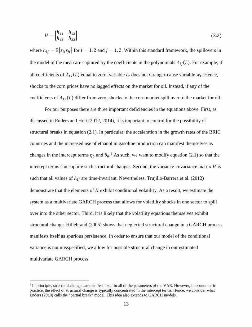
𝐻𝐻 = �ℎ11 ℎ12ℎ12 ℎ22
� (2.2)
where ℎ𝑖𝑖𝑖𝑖 = 𝔼𝔼�𝜀𝜀𝑖𝑖𝑡𝑡𝜀𝜀𝑖𝑖𝑡𝑡� for 𝑖𝑖 = 1, 2 and 𝑗𝑗 = 1, 2. Within this standard framework, the spillovers in
the model of the mean are captured by the coefficients in the polynomials 𝐴𝐴𝑖𝑖𝑖𝑖(𝐿𝐿). For example, if
all coefficients of 𝐴𝐴12(𝐿𝐿) equal to zero, variable 𝑐𝑐𝑡𝑡 does not Granger-cause variable 𝑤𝑤𝑡𝑡. Hence,
shocks to the corn prices have no lagged effects on the market for oil. Instead, if any of the
coefficients of 𝐴𝐴12(𝐿𝐿) differ from zero, shocks to the corn market spill over to the market for oil.
For our purposes there are three important deficiencies in the equations above. First, as
discussed in Enders and Holt (2012, 2014), it is important to control for the possibility of
structural breaks in equation (2.1). In particular, the acceleration in the growth rates of the BRIC
countries and the increased use of ethanol in gasoline production can manifest themselves as
changes in the intercept terms 𝜂𝜂0 and 𝛿𝛿0.6 As such, we want to modify equation (2.1) so that the
intercept terms can capture such structural changes. Second, the variance-covariance matrix 𝐻𝐻 is
such that all values of ℎ𝑖𝑖𝑖𝑖 are time-invariant. Nevertheless, Trujillo-Barrera et al. (2012)
demonstrate that the elements of 𝐻𝐻 exhibit conditional volatility. As a result, we estimate the
system as a multivariate GARCH process that allows for volatility shocks in one sector to spill
over into the other sector. Third, it is likely that the volatility equations themselves exhibit
structural change. Hillebrand (2005) shows that neglected structural change in a GARCH process
manifests itself as spurious persistence. In order to ensure that our model of the conditional
variance is not misspecified, we allow for possible structural change in our estimated
multivariate GARCH process.
6 In principle, structural change can manifest itself in all of the parameters of the VAR. However, in econometric practice, the effect of structural change is typically concentrated in the intercept terms. Hence, we consider what Enders (2010) calls the “partial break” model. This idea also extends to GARCH models.
14
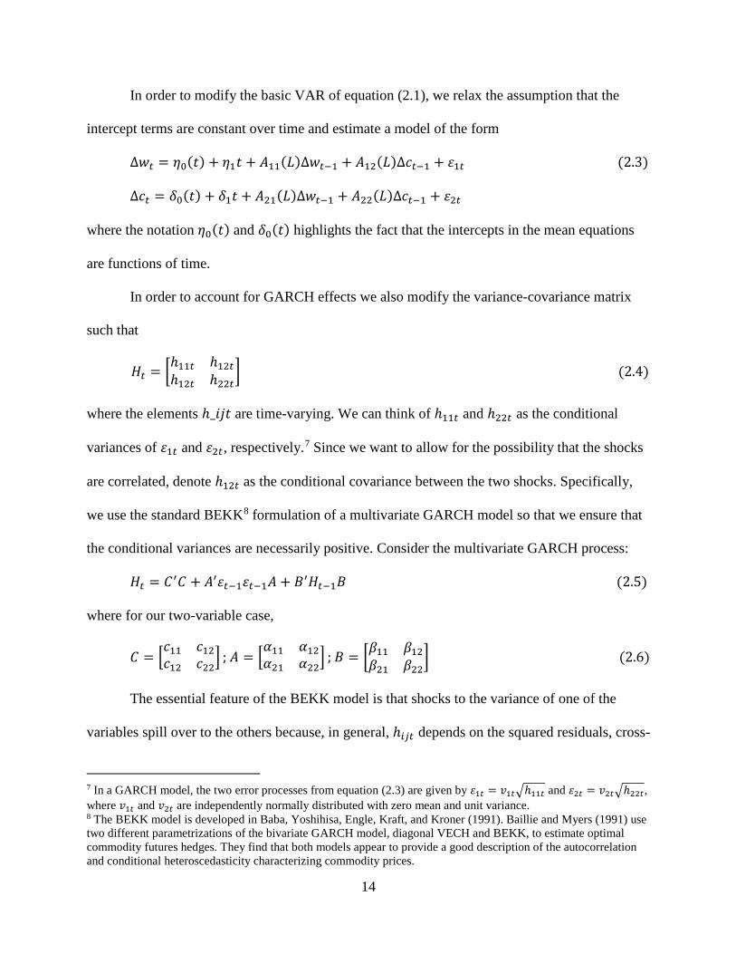
In order to modify the basic VAR of equation (2.1), we relax the assumption that the
intercept terms are constant over time and estimate a model of the form
∆𝑤𝑤𝑡𝑡 = 𝜂𝜂0(𝑡𝑡) + 𝜂𝜂1𝑡𝑡 + 𝐴𝐴11(𝐿𝐿)∆𝑤𝑤𝑡𝑡−1 + 𝐴𝐴12(𝐿𝐿)∆𝑐𝑐𝑡𝑡−1 + 𝜀𝜀1𝑡𝑡 (2.3)
∆𝑐𝑐𝑡𝑡 = 𝛿𝛿0(𝑡𝑡) + 𝛿𝛿1𝑡𝑡 + 𝐴𝐴21(𝐿𝐿)∆𝑤𝑤𝑡𝑡−1 + 𝐴𝐴22(𝐿𝐿)∆𝑐𝑐𝑡𝑡−1 + 𝜀𝜀2𝑡𝑡
where the notation 𝜂𝜂0(𝑡𝑡) and 𝛿𝛿0(𝑡𝑡) highlights the fact that the intercepts in the mean equations
are functions of time.
In order to account for GARCH effects we also modify the variance-covariance matrix
such that
𝐻𝐻𝑡𝑡 = �ℎ11𝑡𝑡 ℎ12𝑡𝑡ℎ12𝑡𝑡 ℎ22𝑡𝑡
� (2.4)
where the elements ℎ_𝑖𝑖𝑗𝑗𝑡𝑡 are time-varying. We can think of ℎ11𝑡𝑡 and ℎ22𝑡𝑡 as the conditional
variances of 𝜀𝜀1𝑡𝑡 and 𝜀𝜀2𝑡𝑡, respectively.7 Since we want to allow for the possibility that the shocks
are correlated, denote ℎ12𝑡𝑡 as the conditional covariance between the two shocks. Specifically,
we use the standard BEKK8 formulation of a multivariate GARCH model so that we ensure that
the conditional variances are necessarily positive. Consider the multivariate GARCH process:
𝐻𝐻𝑡𝑡 = 𝐶𝐶′𝐶𝐶 + 𝐴𝐴′𝜀𝜀𝑡𝑡−1𝜀𝜀𝑡𝑡−1𝐴𝐴 + 𝐵𝐵′𝐻𝐻𝑡𝑡−1𝐵𝐵 (2.5)
where for our two-variable case,
𝐶𝐶 = �𝑐𝑐11 𝑐𝑐12𝑐𝑐12 𝑐𝑐22� ; 𝐴𝐴 = �
𝛼𝛼11 𝛼𝛼12𝛼𝛼21 𝛼𝛼22� ; 𝐵𝐵 = �𝛽𝛽11 𝛽𝛽12
𝛽𝛽21 𝛽𝛽22� (2.6)
The essential feature of the BEKK model is that shocks to the variance of one of the
variables spill over to the others because, in general, ℎ𝑖𝑖𝑖𝑖𝑡𝑡 depends on the squared residuals, cross-
7 In a GARCH model, the two error processes from equation (2.3) are given by 𝜀𝜀1𝑡𝑡 = 𝑣𝑣1𝑡𝑡�ℎ11𝑡𝑡 and 𝜀𝜀2𝑡𝑡 = 𝑣𝑣2𝑡𝑡�ℎ22𝑡𝑡, where 𝑣𝑣1𝑡𝑡 and 𝑣𝑣2𝑡𝑡 are independently normally distributed with zero mean and unit variance. 8 The BEKK model is developed in Baba, Yoshihisa, Engle, Kraft, and Kroner (1991). Baillie and Myers (1991) use two different parametrizations of the bivariate GARCH model, diagonal VECH and BEKK, to estimate optimal commodity futures hedges. They find that both models appear to provide a good description of the autocorrelation and conditional heteroscedasticity characterizing commodity prices.

15
products of residuals, and the conditional variances and covariances of all variables in the
system.
As it stands, equation (2.5) only captures autoregressive dynamics in the variance-
covariance matrix. In order to allow for structural change in the volatility equations, we now
discuss how to incorporate time-varying intercepts into the ℎ𝑖𝑖𝑖𝑖𝑡𝑡.
2.3.1. Smooth structural change
Bai and Perron (1998) develop a methodology that can be used to test for the presence of
multiple sharp structural breaks in a univariate time-series model. In essence, the methodology
entails estimating the model for every possible combination of breaks and selecting the one that
maximizes the log likelihood function (ℒ∗). Bai and Perron develop the appropriate critical
values for a likelihood ratio test in which ℒ∗is compared to the maximized value of the
likelihood function assuming there are no breaks. The situation is more complicated in a VAR
because a break in one variable (say 𝑤𝑤𝑡𝑡) has the potential to cause mean shifts in all of the other
variables. As such, it becomes difficult to determine whether a perceived break in 𝑤𝑤𝑡𝑡 is due to a
shift in its own parameters or to changes in the parameters of the other variables in the model.
Bai, Lumsdaine and Stock (1998) and Qu and Perron (2007) extend the Bai and Perron (1998)
methodology to allow for the presence of multiple structural breaks in the coefficients and/or in
the variance-covariance matrix of a VAR.
All of these papers assume, however, that the breaks are sharp in that they fully manifest
themselves in a single period. In contrast, the work of Enders and Holt (2014) indicates that
smooth breaks best characterize the linkages in the corn and oil price relationship. After all, the
growth rates of the BRIC countries did not jump to their new higher levels in one particular
quarter and the increased use of ethanol is an ongoing process. As such, we believe it reasonable

16
to model the changes in the VAR coefficients and in the variance-covariance matrix as being
smooth rather than sharp.
Fourier series approximation can capture the behavior of any absolutely integrable
function to any degree of accuracy. Hence, instead of estimating the number, form, and the size
of the breaks, we use Enders and Lee’s (2012a) modification of Gallant’s (1981) Flexible Fourier
Form (FFF) to control for breaks in a VAR. Specifically, Enders and Lee (2012a) demonstrate
that their modification of Gallant’s FFF can mimic a time-series with multiple structural breaks.
Enders and Jones (2015) have shown that the FFF approximation works well in the context of a
VAR. In order to understand the nature of the approximation, let 𝜂𝜂0(𝑡𝑡) in equation (2.3) be
represented by9
𝜂𝜂0(𝑡𝑡) = 𝜂𝜂 + ��𝜙𝜙𝑖𝑖 cos �2𝜋𝜋𝑖𝑖𝑡𝑡𝑇𝑇
� + 𝜓𝜓𝑖𝑖 sin �2𝜋𝜋𝑖𝑖𝑡𝑡𝑇𝑇
��𝑘𝑘
𝑖𝑖=1
(2.7)
where 𝜂𝜂, 𝜙𝜙𝑖𝑖, and 𝜓𝜓𝑖𝑖 are constants, 𝑇𝑇 is the number of observations, and 𝑘𝑘 is a constant that
controls how many cumulative Fourier frequencies are included in the approximation.
The key feature of equation (2.7) is the presence of trigonometric terms cos �2𝜋𝜋𝑖𝑖𝑡𝑡𝑇𝑇� and
sin �2𝜋𝜋𝑖𝑖𝑡𝑡𝑇𝑇�. There are several desirable features of this approximation. In particular, equation (2.7)
nests the linear model, and Gallant and Souza (1991) show that the ordinary least squares
estimates of 𝜙𝜙𝑖𝑖 and 𝜓𝜓𝑖𝑖 in equation (2.7) have a multivariate normal distribution.10 As such, a test
for linearity (that is, whether it is possible to reject the null hypothesis that 𝜙𝜙1 = ⋯ = 𝜙𝜙𝑘𝑘 =
𝜓𝜓1 = ⋯ = 𝜓𝜓𝑘𝑘 = 0) can be conducted using a standard F test. Given that the trigonometric terms
9 We model 𝛿𝛿0(𝑡𝑡) in a similar fashion. 10 Note that Astill et al. (2014) develop the critical values to test for the presence of deterministic Fourier components in a univariate time-series model that is asymptotically robust to the order of integration of the process in question.
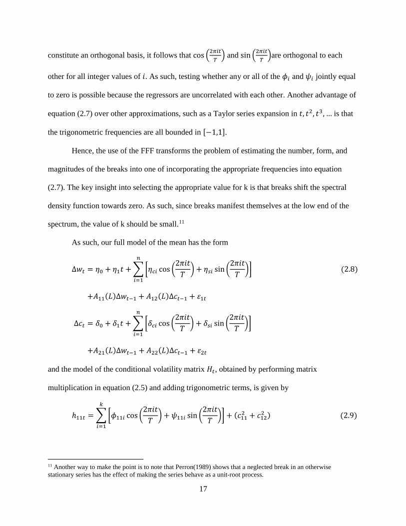
17
constitute an orthogonal basis, it follows that cos �2𝜋𝜋𝑖𝑖𝑡𝑡𝑇𝑇� and sin �2𝜋𝜋𝑖𝑖𝑡𝑡
𝑇𝑇�are orthogonal to each
other for all integer values of 𝑖𝑖. As such, testing whether any or all of the 𝜙𝜙𝑖𝑖 and 𝜓𝜓𝑖𝑖 jointly equal
to zero is possible because the regressors are uncorrelated with each other. Another advantage of
equation (2.7) over other approximations, such as a Taylor series expansion in 𝑡𝑡, 𝑡𝑡2, 𝑡𝑡3, … is that
the trigonometric frequencies are all bounded in [−1,1].
Hence, the use of the FFF transforms the problem of estimating the number, form, and
magnitudes of the breaks into one of incorporating the appropriate frequencies into equation
(2.7). The key insight into selecting the appropriate value for k is that breaks shift the spectral
density function towards zero. As such, since breaks manifest themselves at the low end of the
spectrum, the value of k should be small.11
As such, our full model of the mean has the form
∆𝑤𝑤𝑡𝑡 = 𝜂𝜂0 + 𝜂𝜂1𝑡𝑡 + ��𝜂𝜂𝑐𝑐𝑖𝑖 cos �2𝜋𝜋𝑖𝑖𝑡𝑡𝑇𝑇
� + 𝜂𝜂𝑠𝑠𝑖𝑖 sin �2𝜋𝜋𝑖𝑖𝑡𝑡𝑇𝑇
��𝑛𝑛
𝑖𝑖=1
(2.8)
+𝐴𝐴11(𝐿𝐿)∆𝑤𝑤𝑡𝑡−1 + 𝐴𝐴12(𝐿𝐿)∆𝑐𝑐𝑡𝑡−1 + 𝜀𝜀1𝑡𝑡
∆𝑐𝑐𝑡𝑡 = 𝛿𝛿0 + 𝛿𝛿1𝑡𝑡 + ��𝛿𝛿𝑐𝑐𝑖𝑖 cos �2𝜋𝜋𝑖𝑖𝑡𝑡𝑇𝑇
� + 𝛿𝛿𝑠𝑠𝑖𝑖 sin �2𝜋𝜋𝑖𝑖𝑡𝑡𝑇𝑇
��𝑛𝑛
𝑖𝑖=1
+𝐴𝐴21(𝐿𝐿)∆𝑤𝑤𝑡𝑡−1 + 𝐴𝐴22(𝐿𝐿)∆𝑐𝑐𝑡𝑡−1 + 𝜀𝜀2𝑡𝑡
and the model of the conditional volatility matrix 𝐻𝐻𝑡𝑡, obtained by performing matrix
multiplication in equation (2.5) and adding trigonometric terms, is given by
ℎ11𝑡𝑡 = ��𝜙𝜙11𝑖𝑖 cos �2𝜋𝜋𝑖𝑖𝑡𝑡𝑇𝑇
� + 𝜓𝜓11𝑖𝑖 sin �2𝜋𝜋𝑖𝑖𝑡𝑡𝑇𝑇
�� + (𝑐𝑐112 + 𝑐𝑐122 )𝑘𝑘
𝑖𝑖=1
(2.9)
11 Another way to make the point is to note that Perron(1989) shows that a neglected break in an otherwise stationary series has the effect of making the series behave as a unit-root process.
18
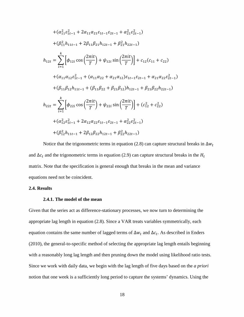
+(𝛼𝛼112 𝜀𝜀1𝑡𝑡−12 + 2𝛼𝛼11𝛼𝛼21𝜀𝜀1𝑡𝑡−1𝜀𝜀2𝑡𝑡−1 + 𝛼𝛼212 𝜀𝜀2𝑡𝑡−12 )
+(𝛽𝛽112 ℎ11𝑡𝑡−1 + 2𝛽𝛽11𝛽𝛽21ℎ12𝑡𝑡−1 + 𝛽𝛽212 ℎ22𝑡𝑡−1)
ℎ12𝑡𝑡 = ��𝜙𝜙12𝑖𝑖 cos �2𝜋𝜋𝑖𝑖𝑡𝑡𝑇𝑇
� + 𝜓𝜓12𝑖𝑖 sin �2𝜋𝜋𝑖𝑖𝑡𝑡𝑇𝑇
�� + 𝑐𝑐12(𝑐𝑐11 + 𝑐𝑐22)𝑘𝑘
𝑖𝑖=1
+(𝛼𝛼11𝛼𝛼12𝜀𝜀1𝑡𝑡−12 + (𝛼𝛼11𝛼𝛼22 + 𝛼𝛼21𝛼𝛼12)𝜀𝜀1𝑡𝑡−1𝜀𝜀2𝑡𝑡−1 + 𝛼𝛼21𝛼𝛼22𝜀𝜀2𝑡𝑡−12 )
+(𝛽𝛽11𝛽𝛽12ℎ11𝑡𝑡−1 + (𝛽𝛽11𝛽𝛽22 + 𝛽𝛽21𝛽𝛽12)ℎ12𝑡𝑡−1 + 𝛽𝛽21𝛽𝛽22ℎ22𝑡𝑡−1)
ℎ22𝑡𝑡 = ��𝜙𝜙22𝑖𝑖 cos �2𝜋𝜋𝑖𝑖𝑡𝑡𝑇𝑇
� + 𝜓𝜓22𝑖𝑖 sin �2𝜋𝜋𝑖𝑖𝑡𝑡𝑇𝑇
�� + (𝑐𝑐122 + 𝑐𝑐222 )𝑘𝑘
𝑖𝑖=1
+(𝛼𝛼122 𝜀𝜀1𝑡𝑡−12 + 2𝛼𝛼12𝛼𝛼22𝜀𝜀1𝑡𝑡−1𝜀𝜀2𝑡𝑡−1 + 𝛼𝛼222 𝜀𝜀2𝑡𝑡−12 )
+(𝛽𝛽122 ℎ11𝑡𝑡−1 + 2𝛽𝛽12𝛽𝛽22ℎ12𝑡𝑡−1 + 𝛽𝛽222 ℎ22𝑡𝑡−1)
Notice that the trigonometric terms in equation (2.8) can capture structural breaks in ∆𝑤𝑤𝑡𝑡
and ∆𝑐𝑐𝑡𝑡 and the trigonometric terms in equation (2.9) can capture structural breaks in the 𝐻𝐻𝑡𝑡
matrix. Note that the specification is general enough that breaks in the mean and variance
equations need not be coincident.
2.4. Results
2.4.1. The model of the mean
Given that the series act as difference-stationary processes, we now turn to determining the
appropriate lag length in equation (2.8). Since a VAR treats variables symmetrically, each
equation contains the same number of lagged terms of ∆𝑤𝑤𝑡𝑡 and ∆𝑐𝑐𝑡𝑡. As described in Enders
(2010), the general-to-specific method of selecting the appropriate lag length entails beginning
with a reasonably long lag length and then pruning down the model using likelihood ratio tests.
Since we work with daily data, we begin with the lag length of five days based on the a priori
notion that one week is a sufficiently long period to capture the systems’ dynamics. Using the

19
significance level of five percent, the general-to-specific procedure results in optimal lag length
of one day for the system of short-term crude oil and corn futures.12 For the system of long-term
futures, the general-to-specific algorithm optimally selects the lag length of five days.
We next determine the number of Fourier frequencies to include in the models of the
mean, equation (2.8), using the general-to-specific method. We begin with five cumulative
trigonometric frequencies (𝑛𝑛 ≤ 5) so that we do not estimate a large number of unnecessary
parameters and because structural breaks manifest themselves in the low end of the spectrum.
The general-to-specific method indicates that five cumulative trigonometric frequencies should
be included in the model of the short-term futures (reducing the number of frequencies from five
to four produces a likelihood ratio test statistic with marginal significance level of 0.038) and in
the model of the long-term futures (0.021). Consequently, when we turn to estimating the models
of the variance we use five Fourier frequencies in our models of the mean for both short- and
long-term futures.
A properly specified model of the mean is essential in assessing the extent to which the
error terms exhibit conditional heteroscedasticity. To this end, we employ a series of diagnostic
tests to ensure that our VAR in equation (2.8) adequately captures all of the dynamics in the
relationship between logarithmic changes of oil and corn futures prices. These tests indicate that
our models of the mean for both short-term and long-term futures capture the autoregressive
effects sufficiently well. For instance, the Ljung-Box Q-statistics for the residuals from each
equation in the short-term model of the mean are 𝑄𝑄(5) = 7.180 and 𝑄𝑄(10) = 10.185 for oil,
and 𝑄𝑄(5) = 1.277 and 𝑄𝑄(10) = 9.598 for corn. None of these statistics are significant at any
12 Use of alternative significance levels of one and ten percent sometimes results in the different number of lags, but our main results are unaffected by the change.

20
conventional level, indicating that the residuals from our short-term VAR display no significant
sample autocorrelations.
Having ensured that our models of the mean properly capture the autoregressive
dynamics in the data, we turn to formal tests for autoregressive conditional heteroscedasticity
(ARCH). For the short-term futures, the Ljung-Box Q-statistics for the squared residuals are
𝑄𝑄(5) = 855 and 𝑄𝑄(10) = 1467 for oil, and 𝑄𝑄(5) = 687 and 𝑄𝑄(10) = 1106 for corn, which
are all highly significant at any conventional level. Not surprisingly, performing the McLeod-Li
(1983) test using a lag length of five days, we find that the value of the test statistic is 𝑇𝑇𝑅𝑅2 =
540 for oil and 𝑇𝑇𝑅𝑅2 = 440 for corn. The magnitudes of the Ljung-Box and McLeod-Li tests
statistics for the long-term futures are similar. Therefore, there is strong evidence of ARCH
errors in the models of the mean for both short-term and long-term futures.
2.4.2. The model of the variance
Given that the error terms in the models of the mean for the short-term and long-term
futures exhibit conditional heteroscedasticity, we now turn to estimating the multivariate
GARCH model given in equation (2.9) that allows for smooth structural changes in volatility;
thus, we address the second and third shortcomings of a basic VAR model that we discuss in the
methods section.
As in the case of the models of the mean, we estimate the models of the variance using up
to five cumulative trigonometric frequencies (i.e., 𝑘𝑘 ≤ 5) in equation (2.9).13 Keep in mind that
inclusion of trigonometric terms in the variance equations accounts for possible structural
changes in conditional volatility, whereas we have already captured possible structural changes
13 Parameter estimates from these models are available from the authors upon request.

21
in the means of the series by selecting appropriate models of the mean for the short-term and
long-term futures in the previous section.
Comparing the model with only one trigonometric frequency, 𝑘𝑘 = 1, to the model with
no trigonometric terms, the estimates suggest that the trigonometric terms are statistically
significant in both the short-term and long-term futures models: the likelihood ratio test statistic
is significant at any conventional level. Thus, we can conclude that there are structural changes
in the conditional volatility of the series and that inclusion of trigonometric terms helps account
for these changes.
Whereas it is clear that the model with only one Fourier frequency is better than the
standard BEKK, models with more cumulative frequencies may offer an even better trade- off
between fit and number of regressors. The likelihood ratio test statistic for 𝑘𝑘 = 5 is not
significant at any conventional level, indicating that the inclusion of Fourier terms with
frequency five to the model that already contains four cumulative frequencies is not warranted.
On the other hand, the statistic for 𝑘𝑘 = 4 is highly significant, suggesting that the restriction that
the coefficients of trigonometric terms with frequency four are equal to zero is binding when
compared against the model with three cumulative Fourier frequencies. Therefore, the general-
to-specific method points to the model with 𝑘𝑘 = 4. For the long-term futures, the general-to-
specific method also suggests the model with four cumulative Fourier frequencies.
Examining the estimated variance equations, we find that the autoregressive coefficients
become smaller after we include trigonometric terms in the model. This observation is consistent
with Hillebrand’s (2005) finding that neglected structural change in a GARCH model manifests
itself as spurious persistence: Fourier terms in our models help account for structural change, so
that the models display less persistence.

22
We use the models with the optimal number of Fourier frequencies in the mean and
variance equations (𝑛𝑛 = 5, 𝑘𝑘 = 4 for both the short- and long-term models) to perform a series
of diagnostic tests. These diagnostic tests reveal that the model of the mean remains properly
specified as we cannot reject the null hypothesis that the various Q-statistics for the standardized
residuals sequences are equal to zero. We test for remaining GARCH effects and find that for
both short- and long-term futures the estimated residuals from the corn equation do not display
any remaining conditional volatility, whereas the residuals from the oil equation do.
Interestingly, the inclusion of the Fourier terms in the variance equations attenuates the problem
of remaining GARCH effects. For example, the Q-statistic for the squared standardized residuals
sequence from the oil equation in the short-term model decreases from 𝑄𝑄(10) = 26.969 to
𝑄𝑄(10) = 22.095 (note that the one percent critical value is 23.21) when we include four
trigonometric frequencies in the variance equations.
2.4.3. Structural changes in volatility
After we estimate our GARCH models with the optimum number of Fourier terms in the
mean and variance equations (five Fourier frequencies in the mean and four in the variance), we
can obtain the predicted values of the conditional volatility series. Specifically, we use the
estimated coefficients and equation (2.9) to obtain predicted values for crude oil conditional
variance, ℎ�11𝑡𝑡, corn conditional variance, ℎ�22𝑡𝑡, and conditional covariance, ℎ�12𝑡𝑡. We construct
the estimates of conditional correlation as follows
𝜌𝜌�12𝑡𝑡 =ℎ�12𝑡𝑡
�ℎ�11𝑡𝑡ℎ�22𝑡𝑡
(2.10)
In addition to estimated conditional volatility series, we obtain the values of the time-varying
intercepts from each member equation in equation (2.9). Since the long-run mean of the series

23
can be found by scaling the intercept by a function of the autoregressive coefficients from the
model, which is a constant, the time-varying intercept is equal to the time-varying long-run mean
of the series up to a multiplicative constant. Note that if we did not include trigonometric terms
in the variance equations, the intercepts (and the long-run means of the series) would be constant
over time. Thus, the time-variation in the intercepts indicates shifts in the long-run means of the
series.
In Panels (a), (b), (c) of Figure 2.2, we plot the estimated conditional volatility series
from the short-term futures model while overlaying the time-varying intercept from each
equation in (9) on the second axis. Looking at the intercept plot in Panel (a), we note that the
long- run mean of the crude oil futures volatility seems to have experienced an increase during
the period from 1997 to 1999 and since then has been on a slow, but steady decline, returning to
pre-1997 levels in 2013. The autoregressive behavior accounted for most of the transient spikes
in crude oil conditional volatility, including the sharp increase in 2008-2009.
Panel (b) indicates that the long-run mean of the corn futures volatility has been steadily
increasing from 2001 to 2010, with accelerated growth beginning in 2006. Therefore, the corn
futures market began experiencing accelerated volatility growth well before the onset of the
crisis in financial markets. An important difference between the crude oil and corn futures
markets is that in the corn market the increased volatility levels associated with the financial
crisis of 2008 were to a larger degree explained by a shift in the long-run mean of the conditional
variance, compared to the oil market.
Turning to the correlation plot in Panel (c), we note that the two markets appear to have
been weakly related until 2007: the correlation coefficient stayed positive most of the time, but
rarely exceeded 0:25. Starting in 2007, the correlation between the two markets increased rapidly

24
and stayed around 0.50 until 2010, experiencing a short, but steep decline in 2010, before
returning to the financial crisis levels until 2012. The correlation since declined to pre-crisis
levels. Comparing the estimated correlation series to its time-varying intercept, we note that the
shifts in the intercept closely mimic the shifts in the series, so that the observed shifts in the
correlation series are for the most part explained by the shifts in its long-run mean, and not by
autoregressive behavior. Given that the beginning of the increase in the correlation coefficient
roughly corresponds to the onset of the financial crisis, we are inclined to conclude that the
increased correlation could be a result of increased integration of the two markets due to ethanol
production, as well as a result of systemic effects in the global economy.
In Figure 2.3, we plot the conditional volatility series from the long-term futures model.
In comparison to the same plots for the short-term model, the peaks of volatility series in the
long-term model are somewhat smaller, as well as the average volatility levels; however, the
overall behavior of the series is almost indistinguishable from the short-term model, including
the time-variation in the intercepts. Thus, we can conclude that the long-term crude oil and corn
futures are slightly less volatile than the short-term futures during both normal times and the
episodes of extreme volatility. The nature of correlation between the two markets does not
appear to depend on the maturity of the contracts with the exception that the estimated
correlation series from the long-term model appears to be noisier.14
2.4.4. Variance impulse response function
Hafner and Herwartz (2006) introduce the concept of the volatility impulse response
function (VIRF) for multivariate GARCH models. Here we briefly discuss how the VIRF can be
14 The plots of the data sequences and conditional variances suggest that there are seasonal impulses. Consistent with this observation, we find evidence of annual seasonality with period 22, which corresponds to the number of summers in our sample. Controlling for seasonality does not qualitatively affect our results. A reproduction of our main analyses with seasonal controls is available upon request.
25
constructed before applying the procedure to our data. Since our BEKK formulation can be
easily put into the VECH form, the calculation of the variance impulse responses is not
difficult.15 Specifically, consider the VECH formulation:
𝑣𝑣𝑣𝑣𝑐𝑐ℎ(𝑯𝑯𝑡𝑡) = 𝑪𝑪 + 𝑨𝑨𝑣𝑣𝑣𝑣𝑐𝑐ℎ(𝜀𝜀𝑡𝑡−1𝜀𝜀𝑡𝑡−1′ ) + 𝑩𝑩𝑣𝑣𝑣𝑣𝑐𝑐ℎ(𝑯𝑯𝑡𝑡−1) (2.11)
where 𝑣𝑣𝑣𝑣𝑐𝑐ℎ is the half-vectorization operator that takes a symmetric 𝑛𝑛 × 𝑛𝑛 matrix and converts it
to an 𝑛𝑛(𝑛𝑛+1)2
× 1 vector by arranging the elements of the lower triangular part of the matrix in a
column vector, 𝑪𝑪 is a vector that is a result of half-vectorization of a positive semi-definite
matrix, and 𝑨𝑨 and 𝑩𝑩 are full 𝑛𝑛(𝑛𝑛+1)2
× 𝑛𝑛(𝑛𝑛+1)2
matrices.
Note that we have essentially written out the expressions for the three elements of
𝑣𝑣𝑣𝑣𝑐𝑐ℎ(𝑯𝑯𝑡𝑡) for our two-variable case with trigonometric terms in equation (2.9). The exact
expressions for 𝑪𝑪, 𝑨𝑨 and 𝑩𝑩 that result from putting our BEKK model in VECH form are
available upon request.
As discussed by Hafner and Herwartz (2006), although the recursion governing equation
(2.11) is very similar to the one governing a one-lag VAR in the mean, we cannot use a
standardized set of shocks to obtain variance impulse responses in a GARCH model since the 𝜀𝜀𝑡𝑡
terms enter the equations as an outer-product. Instead, we must use a complete vector of shocks
to calculate the VIRF. Hafner and Herwarz (2006) offer several interesting ways to create the
vector of shocks to enter into the recursion. For the impulse responses to make sense, these
shocks must somehow be representative of the data. In our analysis, we pick a vector of shocks,
𝜀𝜀𝑡𝑡, that corresponds to a date of some significance.
15 The VECH formulation is named after the 𝑣𝑣𝑣𝑣𝑐𝑐ℎ operator described in the text.

26
Given the chosen vector of shocks, using equation (2.11) we can can construct what
Hafner and Herwartz (2006) call the conditional volatility profile by taking the difference
between the forecast corresponding to the chosen vector of shocks and the forecast
corresponding to the zero vector (𝜀𝜀𝑡𝑡 = 0). Specifically, the conditional volatility profile is given
by
𝑣𝑣𝑣𝑣𝑐𝑐ℎ(𝒗𝒗𝑡𝑡+1) = 𝑨𝑨𝑣𝑣𝑣𝑣𝑐𝑐ℎ(𝜀𝜀𝑡𝑡𝜀𝜀𝑡𝑡′) (2.12)
𝑣𝑣𝑣𝑣𝑐𝑐ℎ(𝒗𝒗𝑡𝑡+𝑘𝑘) = (𝑨𝑨 + 𝑩𝑩)𝑣𝑣𝑣𝑣𝑐𝑐ℎ(𝒗𝒗𝑡𝑡+𝑘𝑘−1)
Note that the conditional volatility profile is a function of the model coefficients and the
shock, and not the data. By analogy with the standard impulse response functions in a VAR, the
VIRF is the revision in the forecast due to observing the given shock. Thus, the VIRF is given by
𝑣𝑣𝑣𝑣𝑐𝑐ℎ(𝑽𝑽𝑡𝑡+1) = 𝑨𝑨𝑣𝑣𝑣𝑣𝑐𝑐ℎ(𝜀𝜀𝑡𝑡𝜀𝜀𝑡𝑡′ − 𝑯𝑯𝑡𝑡) (2.13)
𝑣𝑣𝑣𝑣𝑐𝑐ℎ(𝑽𝑽𝑡𝑡+𝑘𝑘) = (𝑨𝑨 + 𝑩𝑩)𝑣𝑣𝑣𝑣𝑐𝑐ℎ(𝑽𝑽𝑡𝑡+𝑘𝑘−1)
where, as before, 𝑯𝑯𝑡𝑡 is the covariance matrix for time 𝑡𝑡. Thus, the shock to the variance is the
amount by which 𝜀𝜀𝑡𝑡𝜀𝜀𝑡𝑡′ exceeds its expected value, so that the VIRF now depends on the data
through 𝑯𝑯𝑡𝑡.
The historical episode that we consider is the financial crisis of 2008. Since we use daily
data, we have to pick a specific day to obtain the vector of shocks to be used for the VIRF. The
collapse of Lehman Brothers on September 15, 2008 marks the beginning of the period of
extreme turbulence in the U.S. financial markets: during the fall of 2008, the S&P 500 recorded
five of its ten worst trading days in history.16 The first of these five came on September 29, 2008
when the S&P 500 closed 8.79 percent lower than the day before after the U.S. House of
Representatives rejected the proposed $700 billion bailout of the financial industry (three days
16 The complete list can be found at http://money.usnews.com/money/personal-finance/ mutual-funds/articles/2012/10/19/october-sell-off-anyone-the-sps-10-worst-trading-days.

27
later the bailout was passed). We use this date to obtain a vector of shocks for the VIRF as the
news of the rejection of the bailout significantly affected both financial and commodity markets.
Figures 2.4 and 2.5 present the volatility impulse responses of the short-term and the
long-term futures to the shock of September 29, 2008. We scale the responses by the historical
variances at the time of the shock in question as recommended by Hafner and Herwartz (2006).
We first focus on the short-term futures VIRF.
In Panels (a), (c), and (e) of Figure 2.4 we plot the impulse responses of the crude oil
variance, corn variance, and covariance to the shock using the estimates from the GARCH model
with the optimal number of Fourier terms in the mean and variance equations (five Fourier
frequencies in the mean and four in the variance). The shock had a significant initial effect on oil
and corn variance as it caused each to increase by roughly 30 percent; however, the diffusion of
the shock differed noticeably between the two markets. Whereas the shock dissipated relatively
quickly in the corn market, almost vanishing after 100 days, it took more than 200 days to
dissipate in the oil market. The effect of the shock on the covariance between the two markets
was even larger than the effect on the individual variances. The covariance initially increased by
more than 60 percent, and the impulse took almost 200 days to dissipate.
In Panels (b), (d), and (f) of Figure 2.4 we plot the impulse responses of the crude oil
variance, corn variance, and covariance to the shock using the estimates from the GARCH model
without any trigonometric terms in the variance equations. The initial effect of the shock on the
individual variances and the covariances remains similar to the case of the GARCH model with
Fourier terms in the variance equations; however, the shock takes much longer to dissipate, still
appearing to have a significant influence on each variance and the covariance even after 200
days. Thus, when we do not control for structural breaks, the volatility impulse responses appear

28
similar to those from integrated GARCH (IGARCH) processes. The presence of the Fourier
frequencies in our GARCH models make the responses far less persistent.
Focusing now on the long-term futures, we find that the volatility impulse responses in
Figure 2.5 closely resemble those of the short-term futures. The initial effect, the diffusion time,
and the notable increases in persistence when switching to the model without Fourier terms are
almost identical for the VIRF of the short-term and the long-term futures. Based on this
observation, we can conclude that the markets perceived the shock of September 29, 2008 to be
profound enough to affect both the short-term and the long-term futures to an equal degree.
2.4.5. Analysis of the term spread
For corn and oil futures, we can construct the term spread as the difference between
logarithmic changes in the long-term contract and the logarithmic changes in the short-term
contract. In order to better assess whether the relationship between corn and oil volatilities
differs across maturities, we repeat our analysis using the term spread in corn and oil futures.
Specifically, we begin by selecting the optimal lag length in the model of the mean for the
spread. Following the lag selection procedure we used in Section 2.4.2, we find that the optimal
lag length is five days, just as in the case of long-term oil and corn futures. Next, we estimate six
models of the mean by varying the number of included Fourier frequencies from zero to five.
The general-to-specific method indicates that trigonometric terms do not belong in the model of
the mean.
We can conclude that there were no significant structural changes in the spread between
the long-term and the short-term futures prices during our sample period. In other words, the
short-term and the long-term futures price series tend to co-break. Structural shifts seem to affect
the whole term-structure of futures prices, which is consistent with the interpretation of structural

29
change as a long-run effect, so that the markets do not expect the effect to dissipate by the
expiration date of the long-term futures contract.
Using the specification with five lags and no Fourier frequencies as the model of the
mean, we run diagnostic tests to confirm that the error terms exhibit conditional
heteroscedasticity, so that it is appropriate to estimate the relationship between the oil futures
spread and the corn futures spread as a GARCH process. Thus, we estimate six GARCH models
using equations (2.8) and (2.9) by varying the number of trigonometric frequencies included in
the variance equations from zero to five. The general-to-specific method selects the model with
four Fourier frequencies at the one percent level, indicating that volatility breaks are present in
the system of corn and oil futures term spreads.
Our results paint an interesting picture: while structural shifts in the short-term and the
long-term futures prices are statistically indistinguishable, the same does not apply to structural
breaks in the volatility. This effect is consistent with the findings of Brooks (2012) that corn and
crude oil futures markets appear to be unarbitraged. If the markets were arbitraged, we would
expect a flat term structure of futures volatility as shown by Brooks (2012). In turn, this implies
that any structural change experienced by the volatility of the short-term contract would have to
be mimicked by the long-term contract, which we do not observe.
2.5. Conclusion
The purpose of the paper is to examine the interrelationships between prices in the
petroleum and grain markets. Grain prices have always reflected the effects of petroleum prices
on transport and on fertilizers (since most fertilizers require petroleum or natural gas to
manufacture). However, intuition suggests that the interactions between them have become
tighter as a result of the increased importance of the BRIC countries and the regulations

30
requiring increased ethanol production. However, the interactions are not necessarily
unidirectional in that the new biofuel technologies mean that grain prices should be reflected in
petroleum markets. Nevertheless, researchers such as Myers et al. (2014) and Wetzstein and
Wetzstein (2011), contend that impediments like adjustment costs, capacity constraints, and
uncertainties imply that short-run price interactions should be weak.
In order to disentangle the two arguments, we utilize a technique allowing for smooth
shifts in the price relationships between the two markets. Specifically, we model the interaction
between corn and crude oil futures prices as a bivariate GARCH process allowing for smooth
structural change in both the mean and variance/covariance matrix. Toward this end, we expand
the work of Enders and Holt (2012), Trujillo-Barrera et al. (2012), Enders and Lee (2012a), Bai,
Lumsdaine and Stock (1998), Qu and Perron (2007) and Bai and Perron (1998) by using a
Fourier series approximation to account for the slow shifts in a multivariate GARCH model of
corn and oil prices. Specifically, we generalize the Baillie and Morana (2009) and Enders and
Jones (2015) methodologies by incorporating several low frequency trigonometric components
of a Fourier series approximation into the mean and conditional variance equations of a bivariate
GARCH model.
Our key finding is that the opposing viewpoints on the degree of interaction between
petroleum and corn prices each have some validity. In the early part of our sample, the
conditional correlation between innovations in the two markets is generally below 0.25.
Beginning in 2007 there was a sustained increase in the correlation that can be explained by the
traditional view expressed in Enders and Holt (2014) and Trujillo-Barrera et al. (2012). In
essence, the adoption of ethanol standards and the uncertainty resulting from the financial crisis
likely manifested itself in increase in the conditional correlation. After reaching a peak of more

31
than 0.5 in 2010, the conditional correlation began to decline back toward its pre-2007 average.
Hence, we also support the view of Myers et al. (2014), Wetzstein and Wetzstein (2011), Hertel
and Beckman (2010), and Tyner (2010) that the relationship is likely to weaken for a number of
reasons.
Neglected structural change in the mean and/or variance-covariance matrix typically
results in overstated persistence of parameters. We show that our use of the Flexible Fourier
Form to control for structural change leads to quicker shock dissipation in the variance impulse
response function. Compared to a standard multivariate GARCH model without smooth breaks,
our model with Fourier terms indicates that the markets adjust far more rapidly. Specifically, we
construct the variance impulse response function to the shock of September 29, 2008 (the date of
the initial rejection by the U.S. House of Representatives of the proposed $700 billion bailout of
the financial industry) and find that the number of days required for the shock to dissipate more
than doubles when we use the model that does not control for structural change in volatility
compared to the model that does. Noting that this shock happened during the time of a
significant shift in the variance-covariance matrix, we emphasize that the danger of
overestimating the effect of shocks to volatility is greatest during the time of a long-term change
in the volatility structure. It is important to note that controlling for structural change mitigates
the potential problem of spurious persistence often found in bivariate GARCH models.
Finally, our data set allows us to investigate the relationship of corn and oil futures along
the maturity dimension. We find that the structural change in the variance-covariance matrix is
present in both the short-term and the long-term futures. When we focus on the spread between
the long-term futures price and the short-term futures price for each commodity, we find that
there are structural changes in the variance equations in the GARCH model of the term spreads,

32
indicating that the variance-covariance matrices of the short-term and the long-term futures do
not co-break. In other words, the term structures of volatility in these markets, including the
correlation term structure, change over time. This is further evidence that the U.S. corn and crude
oil futures markets are unarbitraged, so that the term-structure of volatility in each market is not
flat. On the other hand, there are no structural breaks in the model of the mean of terms spreads,
hinting that the term structure of futures prices in the corn and oil markets does not change over
time.

33
2.6. References
Astill, S., Harvey, D. I., Leybourne, S. J., & Taylor, A. M. (2015). Robust and powerful tests for nonlinear deterministic components. Oxford Bulletin of Economics and Statistics, 77(6), 780–799.
Bai, J., Lumsdaine, R. L., & Stock, J. H. (1998). Testing for and dating common breaks in
multivariate time series. The Review of Economic Studies, 65(3), 395–432. Bai, J., & Perron, P. (1998). Estimating and testing linear models with multiple structural
changes. Econometrica, 66(1), 47–78. Baillie, R. T., & Morana, C. (2009). Modelling long memory and structural breaks in conditional
variances: An adaptive FIGARCH approach. Journal of Economic Dynamics and Control, 33(8), 1577–1592.
Baillie, R. T., & Myers, R. J. (1991). Bivariate GARCH estimation of the optimal commodity
futures hedge. Journal of Applied Econometrics, 6(2), 109–124. Baba, Y., Engle R., Kraft, D., & Kroner, K. (1991). Multivariate simultaneous generalized
ARCH. Discussion paper, 89–57, Department of Economics: UCSD. Brooks, R. (2012). Samuelson hypothesis and carry arbitrage. The Journal of Derivatives, 20(2),
37–65. Brunetti, C., & Gilbert, C. L. (2000). Bivariate FIGARCH and fractional cointegration. Journal
of Empirical Finance, 7(5), 509–530. Enders, W. (2010). Applied econometric time series. John Wiley and Sons. Enders, W., & Holt, M. T. (2012). Sharp breaks or smooth shifts? An investigation of the
evolution of primary commodity prices. American Journal of Agricultural Economics, 94(2), 659–673.
Enders, W., & Holt, M. T. (2014). The evolving relationships between agricultural and energy
commodity prices: a shifting-mean vector autoregressive analysis. In J. P. Chavas, D. Hummels, and B. Wright, eds. The Economics of Food Price Volatility (pp. 135–87). University of Chicago Press.
Enders, W., & Jones, P. (2016). Grain prices, oil prices, and multiple smooth breaks in a VAR.
Studies in Nonlinear Dynamics and Econometrics, 20(4), 399-419.

34
Enders, W., & Lee, J. (2012a). A unit root test using a Fourier series to approximate smooth breaks. Oxford Bulletin of Economics and Statistics, 74(4), 574–599.
Enders, W., & Lee, J. (2012b). The flexible Fourier form and Dickey–Fuller type unit root tests.
Economics Letters, 117(1), 196–199. Gallant, A. R. (1981). On the bias in flexible functional forms and an essentially unbiased form:
the Fourier flexible form. Journal of Econometrics, 15(2), 211–245. Gallant, A. R., & Souza, G. (1991). On the asymptotic normality of Fourier flexible form
estimates. Journal of Econometrics, 50(3), 329–353. Hafner, C. M., & Herwartz, H. (2006). Volatility impulse responses for multivariate GARCH
models: An exchange rate illustration. Journal of International Money and Finance, 25(5), 719–740.
Hertel, T. W., & Beckman, J. (2011). Commodity price volatility in the biofuel era: an
examination of the linkage between energy and agricultural markets. In The Intended and Unintended Effects of US Agricultural and Biotechnology Policies (pp. 189–221). University of Chicago Press.
Hillebrand, E. (2005). Neglecting parameter changes in GARCH models. Journal of
Econometrics, 129(1), 121–138. Jin, H. J., & Frechette, D. L. (2004). Fractional integration in agricultural futures price
volatilities. American Journal of Agricultural Economics, 86(2), 432–443. Muhammad, A., & Kebede, E. (2009). The emergence of an agro-energy sector: Is agriculture
importing instability from the oil sector. Choices, 24(1), 12–15. Myers, R. J., Johnson, S. R., Helmar, M., & Baumes, H. (2014). Long-run and short-run co-
movements in energy prices and the prices of agricultural feedstocks for biofuel. American Journal of Agricultural Economics, 96(4), 991–1008.
Perron, P. (1989). The great crash, the oil price shock, and the unit root hypothesis.
Econometrica, 57(6), 1361–1401. Qu, Z., & Perron, P. (2007). Estimating and testing structural changes in multivariate
regressions. Econometrica, 75(2), 459–502. Saghaian, S. H. (2010). The impact of the oil sector on commodity prices: Correlation or
causation? Journal of Agricultural and Applied Economics, 42(03), 477–485. Sumner, D. A. (2009). Recent commodity price movements in historical perspective. American
Journal of Agricultural Economics, 91(5), 1250–1256.
35
Trujillo-Barrera, A., Mallory, M., & Garcia, P. (2012). Volatility spillovers in US crude oil, ethanol, and corn futures markets. Journal of Agricultural and Resource Economics, 37(2), 247–262.
Tyner, W. E. (2010). The integration of energy and agricultural markets. Agricultural
Economics, 41(s1), 193–201. Wetzstein, M., & Wetzstein, H. (2011). Four myths surrounding US biofuels. Energy Policy,
39(7), 4308–4312. Wright, B. D. (2011). The economics of grain price volatility. Applied Economic Perspectives
and Policy, 33(1), 32–58. Zhang, Z., Lohr, L., Escalante, C., & Wetzstein, M. (2009). Ethanol, corn, and soybean price
relations in a volatile vehicle-fuels market. Energies, 2(2), 320–339. Zhang, Z., Lohr, L., Escalante, C., & Wetzstein, M. (2010). Food versus fuel: What do prices tell
us? Energy Policy, 38(1), 445–451.

36
Figure 2.1. Futures Settlement Prices. Panels (a) through (d) present the evolution of short-term and long-term corn and crude oil futures settlement prices throughout our sample period. In each panel, the futures prices are normalized by the price of the contract on June 1, 1993, and the resulting index is plotted on the vertical axis.
(a) Short-Term Crude Oil (b) Long-Term Crude Oil
(c) Short-Term Corn (d) Long-Term Corn

37
Figure 2.2. Estimates of Conditional Variance: Short-Term Futures. Panels (a) through (c) present the estimates of crude oil variance, corn variance, and correlation series for our sample period. The variance estimates are the predicted values from equation (2.9). The correlation estimate is obtained by scaling the covariance estimate by the variance estimates. The time-varying intercept from each equation in equation (2.9) is plotted on the second (right) axis. The evolution of the intercept mimics the evolution of the long-run mean of each series.
(a) Crude Oil Variance
(b) Corn Variance
(c) Correlation Coefficient

38
Figure 2.3. Estimates of Conditional Variance: Long-Term Futures. Panels (a) through (c) present the estimates of crude oil variance, corn variance, and correlation series for our sample period. The variance estimates are the predicted values from equation (2.9). The correlation estimate is obtained by scaling the covariance estimate by the variance estimates. The time-varying intercept from each equation in equation (2.9) is plotted on the second (right) axis. The evolution of the intercept mimics the evolution of the long-run mean of each series.
(a) Crude Oil Variance
(b) Corn Variance
(c) Correlation Coefficient

39
Figure 2.4. Variance Impulse Responses: Short-Term Futures. Panels (a) through (e) present the variance impulse responses to the shock of September 29, 2008. Responses in Panels (a), (c), and (e) use the model that includes four Fourier frequencies in the variance equations, whereas responses in the other panels use the model without Fourier terms in the variance equations.
(a) Crude Oil (b) No-Fourier Crude Oil
(c) Corn (d) No-Fourier Corn
(e) Covariance (f) No-Fourier Covariance

40
Figure 2.5. Variance Impulse Responses: Long-Term Futures. Panels (a) through (e) present the variance impulse responses to the shock of September 29, 2008. Responses in Panels (a), (c), and (e) use the model that includes four Fourier frequencies in the variance equations, whereas responses in the other panels use the model without Fourier terms in the variance equations.
(a) Crude Oil (b) No-Fourier Crude Oil
(c) Corn (d) No-Fourier Corn
(e) Covariance (f) No-Fourier Covariance
41
CHAPTER 3: THE INFORMATION IN GLOBAL INTEREST RATE FUTURES CONTRACTS
3.1. Introduction
Studying cross-country differences in the information content of the interest rate term
structure is important to policymakers and entities involved in the international trade and finance
since differences in the yield curve are linked to exchange rate movements and excess currency
returns (Chen and Tsang, 2013). Interest rate futures contracts are tied to the average of select
interest rates based on the loans funded between two entities. Although these contracts reflect
market expectations of future rates, they also contain other information, such as anticipated
default and differing term premiums.
Estrella and Hardouvelis (1991) show that the U.S. term structure reflects monetary-
policy-independent factors that predict real economic activity. Consequently, the term structure
provides useful information to both private investors and policy makers. Estrella and Mishkin
(1997) likewise find that the inference of real economic activity persists for European
economies. Evidence also suggests that the domestic term structure of one country predicts
future real growth of the economy of another country (Plosser and Geert Rouwenhorst, 1994).
Just as the ability of the term structure to forecast real economic activity and growth in
different countries is important to investors and policy makers, so is the ability of current
forward rates to predict future rate changes and holding period returns in different countries.
However, most of the existing literature on the estimation of term premiums and the information

42
about future rate changes and holding period returns uses data only from a single country, most
often the United States (Wright, 2011).
Studies that do examine the term structure across countries find that there exist global
yield factors that explain significant fractions of a country’s yield curve dynamics (Diebold, Li,
and Yue, 2008). The studies also find that the term premium component of forward rates in the
ten major industrialized countries with independent monetary policies has trended down for the
last 20 years, a phenomenon best explained by lower inflation uncertainty resulting from changes
in monetary policy (Wright, 2011). Consistent with this evidence, Dahlquist and Hasseltoft
(2013) find that international bond returns are predicted not only by local factors, but also by a
global factor closely linked to U.S. bond risk premiums and international business cycles.17
These drive risk premiums and expected short-term interest rates in opposite directions. They
also observe increased correlations between international bond risk premiums over time and
suggest an increase in the integration of markets as a possible explanation.
The goal of this study is to examine the association between the informational content of
the term structure across economies. Evidence suggesting convergence of the informational
content across countries would be consistent with the literature on global yield factors and global
financial cycle. Alternatively, evidence suggesting that the term structures of these markets
contain distinct information would suggest that markets participants in difference economies
behave in different ways, perhaps due to difference in macroeconomic conditions or monetary
policy.
17 Existence of a global risk factor and its dependence on macroeconomic conditions in the center country are the two features echoed by the emerging literature on the global financial cycle (Rey, 2015; Miranda-Agrippino and Rey, 2015).

43
We focus our analysis of the term structure on global interest rate futures contracts. There
are two major reasons why the information content of global interest rate futures may vary from
the information content of domestic interest rates. First, the observed rate is based on the futures
market rather than the spot market. Thus, we expect differences between the spot rates and
implied futures rates because informed traders are more likely to trade futures contracts rather
than make interbank transactions. Second, the information content could differ from currency to
currency due to the influence of macroeconomic conditions and government policies. This
prediction is in line with the literature linking macroeconomic indicators and monetary policy to
the term structure. See, for instance, Rudebusch (1995) and Rudebusch and Wu (2008). 18
Rather than impose a factor structure on the yield curve, we investigate time-series
variation in the information content of the term structure by employing simple forecasting
regressions involving forward rates. In this regard, we extend the work of Brooks, Cline, and
Enders (BCE, 2015) by applying their methodology to global interest rate futures contracts. BCE
(2015) explore the informational differences between constant maturity treasury (CMT) yields
and London Interbank Offered Rate (Libor) in the U.S. They extend the work of Brooks, Cline,
and Enders (BCE, 2012), which examines the informational content in Libor spot rates. BCE
(2012) document that during recent periods more information exists in Libor spot rates
concerning future interest rates than expected holding period returns. In their extension, BCE
(2015) document significant differences in the informational content between Libor and CMT.
They also observe that the information content changed significantly as the financial crisis began
and that these changes were related to credit default swap rates and tenor swap rates.
18 Despite its influence, monetary policy does not completely determine the term structure. In fact, the term structure contains useful information beyond what can be explained by monetary policy and macroeconomic indicators (Estrella and Hardouvelis, 1991).

44
Overall, we examine three-month interbank rates in four currencies—United States
Dollar, Euro, Great Britain Pound, and Swiss Franc—and empirically document five unique
results. First, the information contained in implied USD futures rates is significantly different
from the information contained in USD spot rates previously explored by BCE (2015).
Intuitively, implied forward rates derived from Eurodollar futures contracts incorporate
information that differs from information in spot Libor because futures contracts are tied solely
to three-month Libor, whereas USD spot interbank rates address various maturities.
Our second major finding suggests that the four rate-based futures contracts contain
similar information, particularly USD-GBP and GBP-EUR. Moreover, information content of
interest rate futures in the four regions seems to be driven by a single common factor. On the one
hand, differences in macroeconomic conditions and monetary policies could lead to differences
in the information content of interest rate futures. Continued integration of global financial
markets, however, could lessen information differences. Our evidence suggests that the latter
effect tends to dominate.
Third, we show that implied futures rates contain more information regarding rate
changes rather than return premiums. In this respect our findings are similar to BCE (2015);
however, the result is anticipated as the underlying instrument for rate futures is a three-month
interbank rate.
Fourth, information shifts appear highly correlated with macroeconomic conditions and central
bank policies. Our analysis separates implied government policies from the information content
of rate-based futures contracts. The evidence suggests that larger economies contribute more to
information shifts than smaller economies.

45
Finally, we document that significant information shifts occurred during the 2013-2015
time frame. Interestingly, these shifts are more pronounced than those during the great
recessionary period of 2008-2009. By comparison, macroeconomic variables experienced more
widespread structural changes during the financial crisis compared to the 2013-2015 window.
This evidence suggests that information changes during the 2013-2015 period are most likely
explained by either new information generated in rate futures markets, or by the joint diffusive
dynamics between information in these markets and macroeconomic variables. To a smaller
degree, these information changes could be related to structural changes that affected both the
futures markets and the macroeconomies.
The contribution of our findings to the existing literature is in providing distinct evidence
that rate-based futures from four industrialized nations contain similar information. This
evidence is consistent with the findings in Diebold, Li, and Yue (2008), Wright (2011), and
Dahlquist and Hasseltoft (2013). The convergence of the information content, as well as the
finding that larger economies contribute more to information shifts, is also consistent with the
nascent research on the global financial cycle (Rey, 2015). We also uncover a previously
undocumented and surprising information content shift of 2013 – 2015. The shift affected all
four markets and was largely unrelated to macroeconomic fundamentals and monetary policy
indicators, a finding that is consistent with idea that interest rate term structure incorporates
additional information beyond expectations of macroeconomic conditions and the direction of
the monetary policy.

46
3.2. Data and Theoretical Framework
3.2.1. Data
Our examination uses rate-based futures price data provided by Commodity Systems
Incorporated (CSI). We collect all futures contracts that are Eurodollar futures (contract symbol
ED), Euribor futures (contract symbol I), Sterling futures (contract symbol L), and Euroswiss
futures (contract symbol S). A curve-fitting method based on the Nelson and Siegel (1987) and
Svensson (1995) (discussed in detail below) is then used to construct a complete database of
implied monthly discount factors. We use the monthly observations from July 1994 to October
2016 for all analysis.
The four futures markets are similar in that they all trade on the Intercontinental
Exchange (ICE) and are cash settled based on the three-month interbank rate in their respective
currencies: USD for Eurodollar futures, EUR for Euribor futures, GBP for Sterling futures, and
CHF for Euroswiss futures.19 From this point forward we refer to a given contract by its
currency rather than its symbol.
The on-cycle contract expiry months in all four currencies are March, June, September,
and December. With the exception of CHF, contract expiry months also include two to six of the
nearest consecutive calendar months. In all four currencies, contracts expirations extend four to
six years into the future. Trading in a contract with a given expiry month ceases either on the
third Wednesday of that month (GBP), or two London business days prior (USD, EUR, CHF).
The prices of all contracts are quoted as 100 minus the rate of interest, and the contract size is
19 Full contract specifications can be found on the Intercontinental Exchange website. USD: https://www.theice.com/products/31500928/Eurodollar-Futures; EUR: https://www.theice.com/products/38527986/Three-Month-Euribor-Futures; GBP: https://www.theice.com/products/37650330/Three-Month-Sterling-Short-Sterling-Future; CHF: https://www.theice.com/products/37650324/Three-Month-Euro-Swiss-Franc-Euroswiss-Futures.

47
1,000,000 in the contract’s currency with the exception of Sterling futures, where the notional
amount is GBP 500,000.
Final settlement of Eurodollar, Sterling, and Euroswiss futures occurs at 11:00 a.m.
London time on the last trading day of the contract, at which point the contracts are settled based
on ICE Benchmark Administration (IBA) survey of three-month London Interbank Offered Rate
(ICE Libor) in the contracts’ currency. IBA maintains a panel of 11 to 17 contributor banks, and
each ICE Libor rate is calculated using a trimmed arithmetic mean, where the top and bottom
quartiles of contributors’ quotes are excluded from averaging.20
Final settlement of Euribor futures occurs at 10:00 a.m. London time on the last day of
trading. Euriobor futures are settled based on three-month European Money Markets Institute
Euribor Rate (EMMI Euribor). EMMI maintains a panel of 20 contributor banks, whose quotes
are averaged, excluding the top and bottom three quotes.21
Among the four contracts, Eurodollar futures are the most liquid, followed by Euribor,
Sterling, and Euroswiss contracts. In our sample period, average daily volume of trading in the
nearest expiry month is approximately 131 thousand contracts for Eurodollar futures, 75
thousand contracts for Euribor futures, 32 thousand contracts for Sterling futures, and 6,700
contracts for Euroswiss futures. The corresponding notional amounts are USD 131 billion, EUR
75 billion, GBP 16 billion, and CHF 6.7 billion (USD-equivalent amounts are 91 billion for
EUR, 26 billion for GBP, and 5.7 billion for CHF). In all currencies, liquidity monotonically
declines beginning with the fourth nearest expiry month; even so, trading in the more distant
futures contracts remains active with average daily volume in the eighth nearest expiry month
still exceeding USD 77 billion, EUR 21 billion, GBP 7.9 billion, and CHF 261.4 million in
20 Visit https://www.theice.com/iba/libor for additional details on ICE Libor rates. 21 Visit https://www.emmi-benchmarks.eu/euribor-org/about-euribor.html for additional details on EMMI Euribor.

48
notional amount (USD-equivalent amounts are 25.5 billion for EUR, 12.8 billion for GBP, and
220.7 million for CHF).
3.2.2. Theoretical framework
Closely following BCE (2012, 2015), we examine monthly horizons.22 Based on Nelson
and Siegel (1987), Svensson (1995) develops an approach for determining estimates of level,
slope, and multiple curvature terms.23 BCE call this approach the LSC model and express it as
𝑟𝑟�𝜏𝜏𝑖𝑖: 𝑡𝑡𝑖𝑖� = �𝑏𝑏𝑛𝑛,𝑡𝑡𝑖𝑖𝐶𝐶𝑖𝑖,𝑛𝑛(𝜏𝜏𝑖𝑖; 𝑠𝑠𝑛𝑛)𝑁𝑁
𝑛𝑛=0
where
𝐶𝐶𝑖𝑖,0�𝜏𝜏𝑖𝑖; 𝑠𝑠0� = 1
𝐶𝐶𝑖𝑖,1�𝜏𝜏𝑖𝑖; 𝑠𝑠1� =𝑠𝑠1𝜏𝜏𝑖𝑖�1 − exp �−
𝜏𝜏𝑖𝑖𝑠𝑠1��
𝐶𝐶𝑖𝑖,𝑛𝑛�𝜏𝜏𝑖𝑖; 𝑠𝑠𝑛𝑛� =𝑠𝑠𝑛𝑛𝜏𝜏𝑖𝑖�1 − exp �−
𝜏𝜏𝑖𝑖𝑠𝑠𝑛𝑛�� − exp �−
𝜏𝜏𝑖𝑖𝑠𝑠𝑛𝑛� for 𝑛𝑛 > 1
and where 𝑟𝑟�𝜏𝜏𝑖𝑖: 𝑡𝑡𝑖𝑖� denotes the spot interest rate observed at calendar time 𝑡𝑡𝑖𝑖 expressed in years,
with maturity 𝜏𝜏𝑖𝑖, measured in years from 𝑡𝑡𝑖𝑖, and 𝑏𝑏𝑛𝑛,𝑡𝑡𝑖𝑖 denotes the fitted parameters for level,
slope and curvatures. The scalar 𝑠𝑠𝑛𝑛 is deterministic and we require 𝑠𝑠1 = 𝑠𝑠2. The five-parameter
version with four fixed scalars 𝑠𝑠1 = 𝑠𝑠2 = 2.0, 𝑠𝑠3 = 1.0, and 𝑠𝑠4 = 0.5 is applied.24
22 Although the underlying rates all have three-month tenors, with the LSC model we can examine any tenor. For consistency with prior research, we examine one-month tenors. 23 This method is widely supported in the literature. See, for example, Steeley (2008) who examines a variety of term structure estimation methods and finds that this approach is very robust. 24 Since the intercept counts as one parameter, we only need four scalars for a five-parameter model. Several different sets of scalars are examined and have similar results. For the vast majority of our sample, the term structure is relatively smooth and a five-factor model is more than adequate to achieve an accurate fit.

49
The information in the term structure of interest rates can be explored in a variety of
ways. Fama (1984a, 1984b, and 2006) shows the forward-spot differential can be decomposed in
the following way
𝑓𝑓�𝜏𝜏𝑖𝑖 , 𝜏𝜏𝑖𝑖−1: 𝑡𝑡𝑖𝑖� − 𝑟𝑟(𝑡𝑡𝑖𝑖) = 𝔼𝔼ti[�̃�𝑟(𝑡𝑡𝑖𝑖 + (𝑗𝑗 − 1)∆𝜏𝜏)]− 𝑟𝑟(𝑡𝑡𝑖𝑖) + 𝔼𝔼ti�𝑅𝑅𝑅𝑅��𝜏𝜏𝑖𝑖: 𝑡𝑡𝑖𝑖 + ∆𝜏𝜏��
+�𝔼𝔼ti�𝑅𝑅𝑅𝑅��𝜏𝜏𝑖𝑖−𝑘𝑘+1: 𝑡𝑡𝑖𝑖 + 𝑘𝑘∆𝜏𝜏� − 𝑅𝑅𝑅𝑅��𝜏𝜏𝑖𝑖−𝑘𝑘+1: 𝑡𝑡𝑖𝑖 + (𝑘𝑘 − 1)∆𝜏𝜏��𝑖𝑖−1
𝑘𝑘=2
for all forward rates 𝑗𝑗, and all time 𝑡𝑡𝑖𝑖, 𝔼𝔼t𝑖𝑖[∙] is the conditional expectation operator over time 𝑡𝑡𝑖𝑖
information, 𝑓𝑓�𝜏𝜏𝑖𝑖 , 𝜏𝜏𝑖𝑖−1: 𝑡𝑡𝑖𝑖� denotes the forward rate between two points in maturity time (𝜏𝜏𝑖𝑖 and
𝜏𝜏𝑖𝑖−1) observed at 𝑡𝑡𝑖𝑖, 𝑟𝑟(𝑡𝑡𝑖𝑖) denotes the one period spot yield to maturity, and 𝑅𝑅𝑅𝑅��𝜏𝜏𝑖𝑖: 𝑡𝑡𝑖𝑖� denotes
the return premium defined as the excess holding period rate of return (ℎ�(𝜏𝜏𝑘𝑘, 𝜏𝜏𝑘𝑘−1: 𝑡𝑡𝑖𝑖 + ∆𝜏𝜏)) over
the current spot rate. BCE (2015) note that the return premium in this context is the profits on a
portfolio of forward contracts (∑ Π�𝐿𝐿𝐿𝐿𝑛𝑛𝐿𝐿(𝜏𝜏𝑘𝑘, 𝜏𝜏𝑘𝑘−1: 𝑡𝑡𝑖𝑖 + ∆𝜏𝜏)𝑖𝑖𝑘𝑘=2 ):
𝑅𝑅𝑅𝑅��𝜏𝜏𝑖𝑖: 𝑡𝑡𝑖𝑖� = ℎ�(𝜏𝜏𝑘𝑘, 𝜏𝜏𝑘𝑘−1: 𝑡𝑡𝑖𝑖 + ∆𝜏𝜏) − 𝑟𝑟(𝑡𝑡𝑖𝑖) = �Π�𝐿𝐿𝐿𝐿𝑛𝑛𝐿𝐿(𝜏𝜏𝑘𝑘, 𝜏𝜏𝑘𝑘−1: 𝑡𝑡𝑖𝑖 + ∆𝜏𝜏)𝑖𝑖
𝑘𝑘=2
= ��𝑓𝑓(𝜏𝜏𝑘𝑘, 𝜏𝜏𝑘𝑘−1: 𝑡𝑡𝑖𝑖) − 𝑓𝑓(𝜏𝜏𝑘𝑘−1, 𝜏𝜏𝑘𝑘−2: 𝑡𝑡𝑖𝑖 + ∆𝜏𝜏)�𝑖𝑖
𝑘𝑘=2
An advantage to using this expression is that it allows the forward-spot differential to be
viewed as a combination of information related to the expected change in spot rates and the
information related to the expected change in the return premium. For a given forward-spot
differential, if the expected change in the spot rate increases, then the expected change in the
return premium must decrease. One important implication of global futures contracts is that the
forward rates can be traded directly, without any need for complex trades based on implied
forward rates. Thus, the existence of a significant return premium would imply profitable trading
50
opportunities with very low transaction costs or trading restrictions (for example, short selling
bans). BCE (2012) provide an overview of the extant literature. Here, we explore the
informational content of global interest rate futures contracts.
3.2.3. Preliminary analysis
Abrantes-Metz and Metz (2012), Abrantes-Metz and Verstein (2013), and Abrantes-
Metz, Judge, and Villas-Boas (2011) document that at the beginning of the 2008-2009 financial
crisis, Libor displayed patters that differed quite dramatically from the other interest rates. By the
end of 2012, several large-scale investigations were underway investigating the alleged
fraudulent manipulation of Libor settings.25 As the scandal unfolded, rate rigging was alleged in
all four markets covered in this paper. This Libor scandal has resulted in some regulators calling
for the termination of Libor calculations altogether resulting in the loss of the valuable
information context discussed in this paper. Based on the scandal, there could be differential
effects of the scandal in each market.
Figure 3.1 illustrates the behavior of the implied one-month rate in each market. Three-
month GBP Libor has the highest average at 3.8%, followed by USD Libor, at 2.9%. The EUR
Libor averaged 2.5% and CHF Libor averaged 1.2%. Not surprisingly, EUR and CHF are the
most highly correlated at 0.93 whereas GBP and CHF are the least correlated at 0.80.26 Although
the rates in each market are distinct, the four markets tend to move together. For example, during
the financial crisis all rates fell dramatically. Over the last seven years, however, the rates have
been less correlated. Specifically, the correlations among the currency pairs are much lower,
25 See “Libor Scandal,” at http://en.wikipedia.org/wiki/Libor_scandal and sources cited therein. Accessed on January 17, 2017. 26 Other correlations: USD, EUR = 0.83; USD, GBP = 0.91; USD, CHF = 0.81, and EUR, GBP = 0.90.

51
except for EUR-GBP, after the end of the Great Recession in June 2009.27 This provides at least
some anecdotal evidence suggesting the informational content can vary between the markets in
some environments and yet be quite similar in other environments.
3.3. Empirical Methods
The purpose of our investigation is to understand the information contained in the term
structure of interest rates as represented in the interest rate futures market. There are several
reasons why the different country’s rates may result in informational differences, including
differing default risk, differing regulatory environments, differing monetary policies, and
differing fiscal policies. Accordingly, we begin with forecasting regressions estimated over a
rolling window to assess long-run changes in the predictive ability of forward rates across
countries and then augment this analysis with formal tests for structural breaks. We also estimate
the degree of co-movement in the predictive ability of forward rates across country pairs using a
bivariate GARCH model. We associate changes in macroeconomic conditions and monetary
policies with future changes in the information content of interest rates by regressing the
coefficients from the forecasting regressions on lagged macroeconomic indicators. Lastly, we
employ principal components analysis to determine whether information content of interest rates
across countries is driven by common factors.
3.3.1. Fama regressions
The following time-series regressions are estimated over a rolling window to assess the
predictive ability of forward rates:28
𝑅𝑅𝑅𝑅�𝜏𝜏𝑖𝑖: 𝑡𝑡𝑖𝑖 + ∆𝜏𝜏� = 𝛼𝛼1 + 𝛽𝛽1�𝑓𝑓�𝜏𝜏𝑖𝑖 , 𝜏𝜏𝑖𝑖−1: 𝑡𝑡𝑖𝑖� − 𝑟𝑟(𝑡𝑡𝑖𝑖)� + 𝜀𝜀𝑡𝑡+1 (Fama Regression 1)
27 Correlations before (after) June 2009 are as follows: USD, EUR = 0.55 (-0.25); USD, GBP = 0.79 (0.09); USD, CHF = 0.62 (-0.43); EUR, GBP = 0.58 (0.79); EUR, CHF = 0.92 (0.70); GBP, CHF = 0.54 (0.42). 28 We follow the BCE’s (2012, 2015) approach that is based on Fama (1984a).
52
𝑟𝑟(𝑡𝑡𝑖𝑖 + (𝑗𝑗 − 1)∆𝜏𝜏) − 𝑟𝑟(𝑡𝑡𝑖𝑖) = 𝛼𝛼2 + 𝛽𝛽2�𝑓𝑓�𝜏𝜏𝑖𝑖 , 𝜏𝜏𝑖𝑖−1: 𝑡𝑡𝑖𝑖� − 𝑟𝑟(𝑡𝑡𝑖𝑖)�
+ηt+τ−1 (Fama Regression 2)
Fama Regression 1 addresses the ability of the current forward-spot differential, 𝑓𝑓�𝜏𝜏𝑖𝑖 , 𝜏𝜏𝑖𝑖−1: 𝑡𝑡𝑖𝑖� −
𝑟𝑟(𝑡𝑡𝑖𝑖), to predict the return premium 𝑅𝑅𝑅𝑅�𝜏𝜏𝑖𝑖: 𝑡𝑡𝑖𝑖 + ∆𝜏𝜏�, whereas Fama Regression 2 addresses the
ability to predict the future change in the one period spot rate 𝑟𝑟(𝑡𝑡𝑖𝑖 + (𝑗𝑗 − 1)∆𝜏𝜏) − 𝑟𝑟(𝑡𝑡𝑖𝑖). The two
slope coefficients are interrelated based on the covariance between the expected return premium
and the expected change in rates. When this covariance is zero and the current expected changes
in return premiums is zero, then 𝛽𝛽1 and 𝛽𝛽2 sum to one. Often these two slope coefficients do not
sum to one, but they are close and hence are negatively correlated.
Under the unbiased expectations hypothesis, forward rates contain no information about
return premiums, they contain information solely about expected rate changes. Thus, the slope
coefficient in Fama Regression 1 would be 0.0 and the slope coefficient in Fama Regression 2
would be 1.0. When return premiums do exist and forward rates contain future expected spot rate
information, both slope coefficients may be greater than 0.0.
Overlapping observations exist in the dependent variable of Fama Regression 2 and
individual contracts could bias the parameter estimated in the longer maturity contracts. Hence,
Fama (1984a) supplements Fama Regressions 1 and 2 with the following regressions:
Π𝐿𝐿𝐿𝐿𝑛𝑛𝐿𝐿�𝜏𝜏𝑖𝑖 , 𝜏𝜏𝑖𝑖−1: 𝑡𝑡𝑖𝑖 + ∆𝜏𝜏� = 𝛼𝛼3 + 𝛽𝛽3�𝑓𝑓�𝜏𝜏𝑖𝑖 , 𝜏𝜏𝑖𝑖−1: 𝑡𝑡𝑖𝑖� − 𝑓𝑓�𝜏𝜏𝑖𝑖−1, 𝜏𝜏𝑖𝑖−2: 𝑡𝑡𝑖𝑖��
+𝜀𝜀𝑡𝑡+1 (Fama Regression 3)
𝑟𝑟(𝑡𝑡𝑖𝑖 + (𝑗𝑗 − 1)∆𝜏𝜏) − 𝑟𝑟(𝑡𝑡𝑖𝑖 + (𝑗𝑗 − 2)∆𝜏𝜏) = 𝛼𝛼4 + 𝛽𝛽4�𝑓𝑓�𝜏𝜏𝑖𝑖 , 𝜏𝜏𝑖𝑖−1: 𝑡𝑡𝑖𝑖� − 𝑓𝑓�𝜏𝜏𝑖𝑖−1, 𝜏𝜏𝑖𝑖−2: 𝑡𝑡𝑖𝑖��
+𝜂𝜂𝑡𝑡+𝜏𝜏−1 (Fama Regression 4)
Fama Regression 3 complements Fama Regression 1 by examining the power of forward
rates to predict holding period returns on adjacent maturities. Fama Regression 4 complements
53
Fama Regression 2 by examining the forecasting power of forward rates on the specific one
period change in the spot rate.
Based on these four regressions, we seek to determine empirically if implied forward
rates contain information about return premiums, 𝑅𝑅𝑅𝑅�𝜏𝜏𝑖𝑖: 𝑡𝑡𝑖𝑖 + ∆𝜏𝜏�, or the future change in the one
period spot rate, 𝑟𝑟(𝑡𝑡𝑖𝑖 + (𝑗𝑗 − 1)∆𝜏𝜏) − 𝑟𝑟(𝑡𝑡𝑖𝑖). Further, we also seek to determine whether the
corresponding values of the 𝛽𝛽𝑖𝑖 display statistically significant breaks across the distinct markets.
For example, evidence that the similar markets suddenly behave very differently in the period of
the fraud may be evidence that certain markets were subject to manipulation. Following prior
research, we employ three different methodologies – rolling window analysis, formal tests for
structural breaks suggested by Bai and Perron (1998), and analysis of conditional correlations
obtained from multivariate GARCH models – to determine if there are changes in the behavior
of the 𝛽𝛽𝑖𝑖 or the behavior of the cross-market differences between the 𝛽𝛽𝑖𝑖.
3.3.2. Rolling window analysis
BCE (2015) argue that a five-year window of monthly observations readily captures any
shifts in the coefficients and retains sufficient power to conduct inferences on the coefficients.
We therefore estimate Fama Regressions 1 through 4 for each interest rate futures market using
60-month rolling windows. For a given estimation window, we obtain the point estimate of the
slope coefficient as well as the ±2 Newey-West standard error confidence interval. In each
iteration, we move the estimation window one month forward by discarding the earliest
observation and updating the most recent observation by one month.
In order to test whether there are statistical differences in the corresponding slope
coefficients across interest rate futures market pairs, we allow for cross-equation correlation of
the residuals by modifying the rolling window analysis similar to BCE (2015). First, we estimate
54
each Fama Regression 𝑖𝑖 = 1, … ,4 as seemingly unrelated regressions (SUR) for each of the
following futures market pairs: USD-EUR, USD-GBP, USD-CHF, GBP-EUR, GBP-CHF, and
EUR-CHF. Second, we let 𝛽𝛽𝑖𝑖𝑥𝑥(𝑡𝑡) and 𝛽𝛽𝑖𝑖𝑦𝑦(𝑡𝑡) be the SUR estimates of the slope coefficient for
each Fama Regression 𝑖𝑖 in a given futures market pair, using observations 𝑡𝑡 − 60 to 𝑡𝑡. Third, we
form the difference 𝑑𝑑𝑖𝑖𝑥𝑥𝑦𝑦(𝑡𝑡) = 𝛽𝛽𝑖𝑖𝑥𝑥(𝑡𝑡) − 𝛽𝛽𝑖𝑖
𝑦𝑦(𝑡𝑡) and the corresponding ±2 standard error confidence
interval. Moving the estimation window forward by one month in each iteration, we trace the
path followed by 𝑑𝑑𝑖𝑖𝑥𝑥𝑦𝑦(𝑡𝑡) and infer any statistically significant jumps in the difference of the
estimated slope coefficients between any two contracts. Such jumps indicate a shift in the
relative information content in a given interest rate futures market pair.
3.3.3. Multiple structural breaks
Rolling window analysis serves as a general diagnostic of structural shifts in the
information content of the futures markets; however, it does not allow for the detection of exact
break dates and the corresponding break sizes, nor does it allow for the estimation of confidence
intervals around each break date. We therefore augment the rolling window analysis with a more
formal procedure for detecting structural shifts suggested by Bai and Perron (1998). It should
also be noted that the Bai and Perron approach has two important limitations compared to the
rolling window analysis: breaks are assumed to be fully revealed within a single period and the
variance of the error process is assumed to be constant across regression segments.
To implement the Bai and Perron procedure, we closely follow BCE (2015), who provide
the technical details; we simply note here that the procedure essentially searches through all
possible break dates and selects the set of break dates that provides the best possible fit. As
standard in the literature, we allow for a maximum of five breaks, impose the restriction that
breaks cannot be closer than 12 months apart, and test the null hypothesis of no breaks against

55
the alternative hypothesis of five breaks using Bai and Perron’s supremum F-test. The critical
values of the test at the 90% and 95% significance levels are 8.50 and 9.12, respectively. If the
null hypothesis of no structural breaks is rejected, we select the appropriate set of breaks using
the Bayesian information criterion (BIC).
We apply the Bai and Perron procedure directly to Fama Regressions 1 through 4 for
each interest rate futures market. We use a modified procedure when testing whether the set of
breaks in one futures market differs from the set of breaks in another. Specifically, for each Fama
Regression i and each futures market pair, we obtain a series of estimates 𝑑𝑑𝑖𝑖𝑥𝑥𝑦𝑦(𝑡𝑡) = 𝛽𝛽𝑖𝑖𝑥𝑥(𝑡𝑡) −
𝛽𝛽𝑖𝑖𝑦𝑦(𝑡𝑡) from the SUR rolling window analysis and then apply the Bai and Perron procedure to this
series. Essentially, we test for breaks in the long-run mean of the 𝑑𝑑𝑖𝑖𝑥𝑥𝑦𝑦(𝑡𝑡) series, which allows us
to determine statistically significant breaks in the relative information content between any two
futures markets.
3.3.4. Time-varying correlations
An alternative method of determining the relative information content changes between
any two futures markets is to calculate time-varying correlation coefficients between the
innovations in each market for each Fama Regression 𝑖𝑖. As in BCE (2015), let us consider the
multivariate GARCH model for the USD-EUR futures market pair and Fama Regression 𝑖𝑖:
𝑢𝑢𝑈𝑈𝑈𝑈𝑈𝑈,𝑡𝑡 = 𝛼𝛼𝑈𝑈𝑈𝑈𝑈𝑈 + 𝛽𝛽𝑈𝑈𝑈𝑈𝑈𝑈𝑣𝑣𝑈𝑈𝑈𝑈𝑈𝑈,𝑡𝑡 + 𝜀𝜀𝑈𝑈𝑈𝑈𝑈𝑈,𝑡𝑡
𝑢𝑢𝐸𝐸𝑈𝑈𝐸𝐸,𝑡𝑡 = 𝛼𝛼𝐸𝐸𝑈𝑈𝐸𝐸 + 𝛽𝛽𝐸𝐸𝑈𝑈𝐸𝐸𝑣𝑣𝐸𝐸𝑈𝑈𝐸𝐸,𝑡𝑡 + 𝜀𝜀𝐸𝐸𝑈𝑈𝐸𝐸,𝑡𝑡
where 𝑢𝑢𝑈𝑈𝑈𝑈𝑈𝑈,𝑡𝑡 and 𝑣𝑣𝑈𝑈𝑈𝑈𝑈𝑈,𝑡𝑡 are the dependent and independent variables in the USD market, and
𝑢𝑢𝐸𝐸𝑈𝑈𝐸𝐸,𝑡𝑡 and 𝑣𝑣𝐸𝐸𝑈𝑈𝐸𝐸,𝑡𝑡 are the respective variables in the EUR market.
The multivariate GARCH specification allows the variance-covariance matrix of the
innovations 𝜀𝜀𝑈𝑈𝑈𝑈𝑈𝑈,𝑡𝑡 and 𝜀𝜀𝐸𝐸𝑈𝑈𝐸𝐸,𝑡𝑡 to be time-varying:

56
�var�𝜀𝜀𝑈𝑈𝑈𝑈𝑈𝑈,𝑡𝑡� cov�𝜀𝜀𝑈𝑈𝑈𝑈𝑈𝑈,𝑡𝑡, 𝜀𝜀𝐸𝐸𝑈𝑈𝐸𝐸,𝑡𝑡�
cov�𝜀𝜀𝑈𝑈𝑈𝑈𝑈𝑈,𝑡𝑡, 𝜀𝜀𝐸𝐸𝑈𝑈𝐸𝐸,𝑡𝑡� var�𝜀𝜀𝐸𝐸𝑈𝑈𝐸𝐸,𝑡𝑡�� = �𝜎𝜎11
(𝑡𝑡) 𝜎𝜎12(𝑡𝑡)𝜎𝜎12(𝑡𝑡) 𝜎𝜎22(𝑡𝑡)�
We can, therefore, specify a time-varying correlation coefficient as
𝜌𝜌(𝑡𝑡) =𝜎𝜎12(𝑡𝑡)
�𝜎𝜎11(𝑡𝑡)𝜎𝜎22(𝑡𝑡)
By estimating a multivariate GARCH model for each Fama Regression 𝑖𝑖 across all
futures market pairs, we obtain a time-varying correlation coefficient for the corresponding pair.
For our results to be consistent between the futures market pairs, we use the same specification
for each set of Fama Regressions. Specifically, we use a standard BEKK(1,1) specification as in
Enders (2010, pp. 178 – 179). If two futures markets are closely related in terms of their
information content, we expect the estimated correlation coefficient between the innovations to
be close to unity. On the other hand, if the estimated values of 𝜌𝜌(𝑡𝑡) deviate from unity, we
conclude that the two markets do not move together with respect to the information content.
3.4. Empirical Results
3.4.1. Individual interest rate futures results
Table 3.1 reports estimates of the number of structural breaks and their corresponding
dates for all four futures markets based on the Bai-Perron procedure. Using the 90% critical
value of the supremum F-test (8.50), we infer no structural breaks for any market in Fama
Regression 4 and no breaks for CHF in Fama Regressions 1 and 3. The remaining markets all
had at least one break during the financial crisis period in each Fama Regression.
Although there were the maximum number of breaks reported for Fama Regression 2 for
all countries, there were no breaks found for Fama Regression 4. Further, more breaks were
found for Fama Regression 3 when compared with Fama Regression 1. Specifically, Fama
Regression 3 breaks were found in the 2003-2005 range—a period absent in Fama Regression 1.

57
Thus, the dominant break information is in Fama Regression 2, but there are interesting results
related to return premiums, particularly incremental return premiums.
Figures 3.2 through 3.5 plot the point estimates and ±2 standard error confidence bands
from rolling window estimation of Fama Regressions 1 through 4, respectively. Each figure
contains four panels representing the four individual rate-based futures markets. We make four
key observations from these four figures.
First, the plots in Panel (a) of Figures 3.2 through 3.5 indicate that USD-based implied
rates contain information significantly different from that presented in BCE (2015). This
difference is driven by the fact that futures contracts are tied solely to three-month Libor whereas
spot USD interbank rates address various maturities. Therefore, implied forward rates derived
from Eurodollar futures contracts contain significantly different information when compared to
spot Libor. Eurodollar futures only reflects three-month Libor, no other tenor is available for all
of these markets.29
Second, although each currency has unique characteristics, the general patterns are
similar across USD, EUR, GBP, and CHF. For example, in Figure 3.2 there is a significant
downward shift in the Fama Regression 1 slope coefficient during the financial crisis as well as a
significant upward move over the 2013-2015 period. Across all panels, a similar but opposite
pattern occurs in Figure 3.3. Combined, this evidence implies that the information content across
USD, EUR, GBP, and CHF implied futures rates is generally consistent, and is in line with the
literature on global yield factors and global financial cycle.
Third, the generally positive and significant slope coefficients observed in Figure 3.3 and
Figure 3.5 indicate that implied futures rates contain more information regarding rate changes
29 In the U.S., there is an active one-month Libor contract.

58
than return premiums. This outcome is intuitive since these futures markets addresses only three-
month rates rather than the rates of various maturities, where maturity-based return premium
should be most pronounced.
Fourth, although a profound shift was expected during the financial crisis, the significant
shift in the 2013-2015 time frame was not. Whatever the driver, it impacted all four Fama
Regressions significantly. For example, Figure 3.2 shows a sharp rise in the slope coefficients
whereas Figure 3.3 shows a sharp fall in the slope coefficients.
3.4.2. Differential beta results
Table 3.2 reports estimates of the number and the timing of structural breaks in the
differential beta based on the Bai-Perron procedure. Interestingly, every market pair has the
maximum allowable number of structural breaks in the differential beta except for GBP-CHF in
Fama Regression 3.
For most pairs, there is a structural break during the great recessionary period. A few
pairs, however, do not have a break between late 2007 and 2009; for example, EUR-CHF in
Fama Regression 1 as well as USD-GBP and USD-CHF in Fama Regression 4. There also
appears to be a significant shift in the differential information content between each of the
futures market pairs during the 2013-2015 period. This shift was more widespread than the
information shift associated with the great recession because each pair experienced a break in
each Fama Regression.
Table 3.3 contains additional information about the differential beta breaks. For each
break, we report the break date and the associated 90% confidence interval, as well as the
differential beta corresponding to the period preceding a given break date. For instance, the
reported 𝑑𝑑𝑖𝑖(𝑡𝑡) = 0.373 for the USD-EUR in Fama Regression 1 is the average differential beta

59
during the period before the first break occurred in December 2000. After the break, the average
differential beta shifts to 𝑑𝑑𝑖𝑖(𝑡𝑡) = −0.592 until the next break occurs in August 2006,
corresponding to the break size of -0.965 (-0.592 minus 0.373). The December 2000 break also
appears to be relatively accurately determined as the confidence interval is narrow (four months
between 2000:10 and 2001:01) compared to some of the other identified breaks, for instance, the
last break in Fama Regression 1 for USD-CHF (between 2009:07 and 2015:04).
We use the estimated break sizes to further investigate the difference between the shift
associated with the financial crisis and the shift during the 2013-2015 time frame. For each
futures market pair and each Fama Regression, we identify the first break that occurred during
either the 2007-2009 period, or the 2013-2015 period, and then calculate the average of the
magnitudes of these breaks. The first breaks that occurred during the financial crisis have an
average magnitude of 0.534, whereas the first breaks that occurred during the 2013-2015 period
have an average magnitude of 0.737. Thus, the 2013-2015 information shift appears to be both
more widespread and more pronounced than the information shift during the financial crisis.
Both shifts appear to be very close in terms timing uncertainty – the average length of the
confidence interval is approximately 9 months for the financial crisis breaks and 8 months for the
2013-2015 breaks.
Figures 3.6 through 3.9 illustrate the point estimates and ±2 standard error confidence
bands for the differential betas for Fama Regressions 1 through 4, respectively. Each figure
contains six panels representing the six pairs of rate-based futures market comparisons. We make
four key observations.
First, overall the differential betas for all four Fama Regressions across the six currency
pairs are rarely significantly different from zero. Thus, whatever information is contained in one
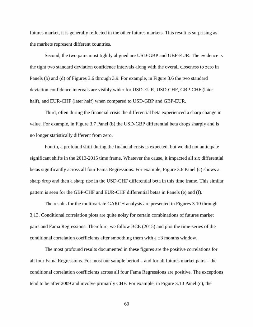
60
futures market, it is generally reflected in the other futures markets. This result is surprising as
the markets represent different countries.
Second, the two pairs most tightly aligned are USD-GBP and GBP-EUR. The evidence is
the tight two standard deviation confidence intervals along with the overall closeness to zero in
Panels (b) and (d) of Figures 3.6 through 3.9. For example, in Figure 3.6 the two standard
deviation confidence intervals are visibly wider for USD-EUR, USD-CHF, GBP-CHF (later
half), and EUR-CHF (later half) when compared to USD-GBP and GBP-EUR.
Third, often during the financial crisis the differential beta experienced a sharp change in
value. For example, in Figure 3.7 Panel (b) the USD-GBP differential beta drops sharply and is
no longer statistically different from zero.
Fourth, a profound shift during the financial crisis is expected, but we did not anticipate
significant shifts in the 2013-2015 time frame. Whatever the cause, it impacted all six differential
betas significantly across all four Fama Regressions. For example, Figure 3.6 Panel (c) shows a
sharp drop and then a sharp rise in the USD-CHF differential beta in this time frame. This similar
pattern is seen for the GBP-CHF and EUR-CHF differential betas in Panels (e) and (f).
The results for the multivariate GARCH analysis are presented in Figures 3.10 through
3.13. Conditional correlation plots are quite noisy for certain combinations of futures market
pairs and Fama Regressions. Therefore, we follow BCE (2015) and plot the time-series of the
conditional correlation coefficients after smoothing them with a ±3 months window.
The most profound results documented in these figures are the positive correlations for
all four Fama Regressions. For most our sample period – and for all futures market pairs – the
conditional correlation coefficients across all four Fama Regressions are positive. The exceptions
tend to be after 2009 and involve primarily CHF. For example, in Figure 3.10 Panel (c), the
61
USD-CHF Fama Regression 1 correlation is positive except for a brief period in the late 1990s
and a significant period starting in 2009. A somewhat similar pattern is observed for GBP-CHF
in Figure 3.10 Panel (e). In Figure 3.11 Panel (c), the results are similar for Fama Regression 2.
Interestingly, the pattern is not the same for USD-GBP in Figure 3.11 Panel (b). The lack of
correlation is particularly pronounced in the later periods. Thus, innovations in USD and GBP
for Fama Regression 2 were not as strongly linked in these latter periods.
3.4.3. Interpreting the results
Our findings suggest that the estimated Fama regression betas from the four different
economies move together. To explore this co-movement, we seek to identify the key factors. We
consider four categories of explanatory variables: interest rate risk premiums, central bank
monetary policy targets, macroeconomic conditions, and business cycle and uncertainty
indicators.
In money markets, the interest rate risk premium variables include measures of the
default premium, term premium, and the liquidity premium. In the wake of the Great
Recession, and the following European debt crisis, there were significant concerns about possible
bank defaults in many European countries. This casted doubt on the Euro as well as Euro-
denominated debt securities. Under these circumstances, the varying default risks across
economies are likely to contribute significantly to variation in beta estimates. We therefore
include credit spreads as a measure of default premium.
Since all futures contracts in our study have the same maturity and the same tenor of the
underlying, we do not explore various term premium measures. In addition, rate-based futures
contracts tend to be very actively traded, so we do not examine liquidity premium variables. We

62
therefore contend that the time-varying default premiums should contain the most explanatory
power with respect to the three risk premium determinants.
One important property of the rate-based futures contracts is that these contracts are cash
settled based on the three-month interbank rate, a rate closely affected by central banks. For
instance, according to the Swiss National Bank (SNB), its monetary policy is implemented by
fixing a target range for the reference interest rate, which is the Libor for three-month interbank
loans in Swiss Francs.30 Clearly, the rate-based futures are heavily affected by the conduct of
government monetary policy. To measure the effect of monetary policy, we consider the central
bank target rate and the month-on-month growth of M1 and include it in the regressions.
Macroeconomic indicators reflecting government monetary policy are also expected to
provide significant explanatory power for our information measures.31 We therefore include the
inflation rate, unemployment rate, and the nominal effective exchange rate (NEER).
Macroeconomic activity or business cycle factors affect not only the risk premium, but
are important determinants of macroeconomic variables such as inflation and unemployment.
Thus, macroeconomic or financial business cycle indicators may be good candidates for
forecasting excess returns on interest rate futures contracts. We therefore include the Purchasing
Managers' index (PMI) and stock market implied volatility (VIX) to capture the effect of the
business cycle and uncertainty.
Table 3.4 reports how the individual betas from the Fama Regressions relate to credit
spreads, government monetary policy, and macroeconomic conditions. To avoid endogeneity
30 More detailed discussion of Swiss monetary policy implementation can be found on its website through the following link: https://www.snb.ch/en/iabout/monpol 31For example, Switzerland, as a small open economy relying heavily on imports, chose to maintain the minimum exchange rate (no further appreciation of CHF) of CHF 1.20 per euro from September 2011 to January 2015.

63
concerns, the explanatory variables are lagged by one month.32 Panels (a) through (d) examine
the univariate betas from Fama Regression 1 through 4, respectively. The Fama Regression betas
are significantly correlated to most macroeconomic factors, including inflation, central bank
target rate, M1 growth rate, unemployment rate, PMI, VIX, and nominal effective exchange rate.
The 𝑅𝑅2 for EUR, GBP, CHF, and USD are approximately 0.5, 0.8, 0.4, and 0.6, respectively,
suggesting a significant portion in the variation in betas is explained by our model. Noticeably,
UK’s model explains 80% of the variation, suggesting effective communication between the
market and UK policymakers. In contrast, the relatively lower 𝑅𝑅2 from the Swiss Franc market is
likely due to the fact that the SNB has a history of surprising the market relative to other
countries.33 Overall, both betas from return premium and rate changes regressions are highly
correlated with macroeconomic conditions and central bank policy goals and targets. From this
perspective, the markets are highly aware of the macroeconomic conditions and central bank
targets, and thus make adjustments accordingly.
Our key finding is that Fama Regression betas follow a similar pattern in all four markets.
Since the markets’ expectations are highly correlated with macroeconomic conditions and central
bank reactions, the common pattern may be due to the fact that the four economies experience
similar macroeconomic shocks and implement monetary policies in a similar manner. To test this
claim, we use two different approaches relying on individual and differential betas, respectively.
32 We are aware of the fact that lagging macroeconomic indicators by one month may not be sufficient because Fama Regression betas are estimated over the prior 60 months. We perform two robustness checks. First, Fama Regression betas are estimated with a 12-month centered rolling window and regressed on 6-month lagged macroeconomic variables. Second, Fama Regression betas are estimated using daily data over disjoint monthly intervals (there is still one beta estimate per month) and regressed on 1-month lagged macroeconomic variables. These results are generally consistent with the baseline results. 33For example, the announcement of SNB to maintain the minimum exchange rate in September 2011 truly surprised the market at the time. The adoption of negative interest rate by SNB in 2015 was also less than expected.

64
First, if the four economies experience similar macroeconomic shocks, then these shocks
are likely due to an underlying global factor (e.g. the 2007-2009 global financial crisis). To
detect this potential common factor, we implement principal component analysis (PCA) on the
individual betas. The goal of PCA is to identify as few components (linear combinations of
individual betas) as possible to capture the sources of variation in the individual betas in the four
markets.34 As shown in Figure 3.14, one single (the largest) component explains most of the
variation in the individual betas from the four Fama regressions. Table 3.5 reports the results of
PCA. The largest component captures a larger share of the total variation in the individual betas
in regressions involving return premiums (91.54% and 93.70% in Fama Regressions 1 and 3,
respectively) than in regressions involving future rate changes (86.17% and 85.66% in Fama
Regressions 2 and 4, respectively). The roughly equal component loadings suggest that the
largest component is a roughly equally weighted linear combination of the four individual betas.
This component therefore represents the average information content of the global market and is
thus a global component, consistent with the literature on global yield factors and global
financial cycle.
Second, we use differential betas to test our claim that the four economies experience
similar macroeconomic shocks and implement monetary policies in a similar manner. Table 3.6
examines how macroeconomic variables impact differential betas across the six economy pairs:
USD-EUR, USD-GBP, USD-CHF, GBP-CHF, GBP-EUR, and EUR-CHF. For each pair, we
regress the differential beta on the relevant economies’ macroeconomic variables. For example,
for the USD-EUR pair, we consider macroeconomic variables in the US and Euro area. To avoid
34 Because we have four markets, a group of four components can fully explain the variation in the individual betas.

65
multicollinearity, we use the US and Euro area macroeconomic variables in separate regressions.
To save space, only the 𝑅𝑅2 is reported.
The results in Table 3.6 suggest that, although each relevant economy does contribute to
differential betas, the contribution is not equal. In particular, the Eurozone contributes more than
the US to USD-EUR beta differential (e.g., Fama Regression 1 𝑅𝑅2of 0.795 compared to 0.462);
the UK contributes more than the US to USD-GBP beta differential; the US contributes more
than the Switzerland to USD-CHF beta differential; the UK contributes more than the
Switzerland to GBP-CHF beta differential; the UK contributes more than the Eurozone to GBP-
EUR beta differential; the Euro area contributes more than the Switzerland to EUR-CHF beta
differential. Overall, as expected, larger economies contribute more to the differential betas with
the exception of USD-GBP and GBP-EUR pairs. One reason for the dominance of the UK could
be the fact that the contracts are based on a rate fixing occurring in London.
Collectively, the Fama Regression betas are highly correlated with macroeconomic
conditions as well as central bank policy targets. This finding highlights the fact that financial
markets reflect economic fundamentals and communicate effectively with policymakers. During
crises, however, there is increased uncertainty regarding economy activity and government
action. Thus, financial market participants have more difficulty forming consistent expectations,
reflecting wider confidence intervals for the Fama Regression betas.
Up to this point we have shown that the time-series behavior of the univariate and
differential Fama Regression betas is significantly related to key macroeconomic and monetary
policy indicators. Both the joint diffusive dynamics and simultaneous structural breaks could be
the drivers of the observed linkage between the information content of interest rate futures (Fama
Regression betas) and macroeconomic indicators. We, therefore, employ the Bai-Perron

66
methodology to determine whether information content changes are consistent with the structural
shifts in the macroeconomic variables and report the results in Table 3.7. We address non-
stationarity of certain macroeconomic variables and allow for a maximum of five breaks except
for the cases where the sample period was limited due to the availability of the data (three breaks
for Eurozone PMI and Switzerland VIX, four breaks for United Kingdom PMI).
Table 3.7 contains the break dates and related information for inflation, policy rate, M1
growth rate, unemployment rate, PMI, VIX, credit spread, and NEER in each of the four
markets. At least some of the economic indicators in each market experienced a structural shift
during the financial crisis, which is consistent with the structural changes in the information
content of interest rate futures during this period. Only a few of the macroeconomic variables
had a structural shift during or near the 2013-2015 window, which is a time when significant
shifts occurred in the interest rate futures markets. These variables include United States
inflation, Eurozone VIX, and United Kingdom inflation, M1 growth rate, and NEER. Thus,
coincidence of structural breaks in interest rate futures and macroeconomic indicators is less
pronounced during the 2013-2015 period than during the financial crisis.
There are three potential explanations of the 2013-2015 phenomenon. First, information
changes in the interest rate futures markets during this time could be due to the arrival of new
information unrelated to the macroeconomic variables that we have considered. Second,
information changes could be due to the joined diffusive dynamics (common shocks to
differential betas and macroeconomic indicators) of macroeconomic indicators and information
content of the rate-based futures. Third, information changes could be due to structural breaks
that have affected both the interest rate futures markets and the macroeconomies, although our
results indicate that this is the less likely explanation.

67
3.5. Conclusion
We examine global interest rate futures contracts with a focus on information content as
revealed by the Fama regressions. We examine differential betas, structural breaks, and time-
varying correlations and empirically document five unique results. First, implied USD futures
rates contain information that significantly differs from previously documented information in
the spot rates. Second, the four rate-based futures contracts contain similar information,
particularly USD-GBP and GBP-EUR, as anticipated based on geographic location and economy
size. Third, given that the underlying is always a three-month rate on interbank deposits, the
implied futures rates contain more information regarding rate changes rather than return
premiums. Fourth, information shifts appear highly correlated with macroeconomic conditions
and central bank policies. Finally, significant information shifts occurred during the 2013-2015
time frame, even greater than during the great recessionary period of 2008-2009.
Collectively, our results indicate that the rate-based futures from four industrialized
nations contain similar information. This evidence is consistent with the findings in Diebold, Li,
and Yue (2008), Wright (2011), and Dahlquist and Hasseltoft (2013). The convergence of the
information content, as well as the finding that larger economies contribute more to information
shifts, is also consistent with the nascent research on the global financial cycle (Rey, 2015).

68
3.6. References
Abrantes-Metz, Rosa M. and Albert D. Metz, 2012. How far can screens go in distinguishing explicit from tacit collusion? New evidence from the Libor setting, CPI Antitrust Chronicle 3.
Abrantes-Metz, Rosa M. and Andrew Verstein, 2013. Revolution in manipulation law: The new
CFTC rules and the urgent need for economic and empirical analyses, University of Pennsylvania Journal of Business Law, 15, 357-418.
Abrantes-Metz, Rosa M., George G. Judge, and Sofia B. Villas-Boas, 2011. Tracking the Libor
rate, Applied Economic Letters, 18, 893-899. Bai, J. and P. Perron, 1998. Estimating and testing linear models with multiple structural
changes, Econometrica 66, 47-78. Brooks, R., B. N. Cline, and W. Enders, 2012. Information in the U.S. Treasury term structure of
interest rates, The Financial Review 47, 247-272. Brooks, R., B. N. Cline, and W. Enders, 2015. A Comparison of the Information in the Libor and
CMT Term Structures of Interest Rates, Journal of Banking and Finance 54, 239-253. Chen, Y. and K. P. Tsang, K. P., 2013. What Does the Yield Curve Tell Us about Exchange Rate
Predictability? Review of Economics and Statistics, 95(1), 185–205. Dahlquist, M. and H. Hasseltoft, 2013. International Bond Risk Premiums, Journal of
International Economics, 90(1), 17–32. Diebold, Francis X., and Canlin Li, 2006. Forecasting the term structure of government bond
yields, Journal of Econometrics 130, 337-364. Diebold, Francis X., Canlin Li, and Vivian Z. Yue, 2008. Global yield curve dynamics and
interactions: A dynamic Nelson-Siegel approach, Journal of Econometrics 146, 351-363. Enders, Walter, 2010. Applied Econometric Time Series. Wiley: Hoboken, N.J. Estrella, A. and G. A. Hardouvelis, 1991. The Term Structure as a Predictor of Real Economic
Activity, The Journal of Finance, 46(2), 555–576.

69
Estrella, A. and F. S. Mishkin, 1997. The predictive power of the term structure of interest rates in Europe and the United States: Implications for the European Central Bank, European Economic Review, 41(7), 1375–1401.
Fama, E. 1984a. The information in the term structure, Journal of Financial Economics 13, 509-
528. Fama, E., 1984b. Term premiums in bond returns, Journal of Financial Economics 13, 529-546. Fama, E., 1986. Term premiums and default premiums in money markets, Journal of Financial
Economics 17, 175-196. Fama, E., 2006. The behavior of interest rates, Review of Financial Studies 19, 359-379. Miranda-Agrippino, S. and H. Rey, 2015. World Asset Markets and the Global Financial Cycle,
NBER Working Paper Series, 21722. Nelson, C. and A. Siegel, 1987. Parsimonious modeling of yield curves, Journal of Business 60,
473-489. Plosser, C. I. and K. Geert Rouwenhorst, 1994. International term structures and real economic
growth, Journal of Monetary Economics, 33(1), 133–155. Rey, H., 2015. Dilemma not Trilemma: The global Financial Cycle and Monetary Policy
Independence, NBER Working Paper Series, 21162. Rudebusch, G. D., 1995. Federal Reserve interest rate targeting, rational expectations, and the
term structure, Journal of Monetary Economics, 35(2), 245–274. Rudebusch, G. D. and T. Wu, 2008. A Macro-Finance Model of the Term Structure, Monetary
Policy and the Economy, The Economic Journal, 118(530), 906–926. Steeley, J., 2008. Testing term structure estimation methods: Evidence from the UK STRIPs
market.” Journal of Money, Credit and Banking 40, 1489-1512. Svensson, L.E.O., 1995. Estimating Forward Interest Rates with the Extended Nelson and Siegel
Method, Sveriges Riksbank Quarterly Review, 1995(3), 13–26. Wright, J. H. (2011). Term Premiums and Inflation Uncertainty: Empirical Evidence from an
International Panel Dataset, The American Economic Review, 101(4), 1514–1534.

70
Table 3.1. Estimated Number of Breaks and Break Dates for Individual Rates. For each market, F(5) is the supremum F-value for the null hypothesis of 5 versus no breaks, Breaks is the estimated number of breaks, Dates are the estimated break dates, BIC(0) is the sample BIC value for the model with no breaks, and BIC(b) is the sample BIC value for the model with the optimal number of breaks. If the F-test indicates no breaks, the BIC is not reported. The smaller the BIC, the better the fit of the model. Market F(5) Breaks Dates BIC(0) /
BIC(b) Fama Regression 1 (Return Premiums)
USD 11.88 4 2000:11 2001:11 2007:12 2008:12 -15.40/-15.58 EUR 11.81 4 1995:06 2007:07 2008:09 2009:09 -15.73/-15.91 GBP 15.00 3 1997:02 2008:09 2009:09 -15.36/-15.61 CHF 5.52 0
Fama Regression 2 (Rate Changes) USD 22.80 5 2000:10 2001:10 2004:02 2007:10 2008:12 -16.28/-16.71 EUR 24.56 5 1995:07 2001:09 2005:06 2008:07 2009:07 -16.58/-17.05 GBP 23.61 5 1998:10 1999:12 2002:08 2008:07 2009:07 -16.16/-16.60 CHF 11.97 5 1996:08 2002:01 2003:04 2008:03 2009:03 -16.33/-16.51
Fama Regression 3 (Incremental Return Premiums) USD 13.92 5 2000:11 2002:03 2004:03 2007:12 2008:12 -17.44/-17.67 EUR 15.27 5 1995:07 2001:11 2005:08 2008:09 2009:09 -17.91/-18.17 GBP 13.65 4 1998:06 2003:02 2008:09 2009:09 -17.43/-17.66 CHF 6.57 0
Fama Regression 4 (Incremental Rate Changes) USD 7.28 0 EUR 6.16 0 GBP 5.56 0 CHF 4.85 0

71
Table 3.2. Estimated Number of Breaks and Break Dates for Rate Pairs. For each market pair, F(5) is the supremum F-value for the null hypothesis of 5 versus no breaks, Breaks is the estimated number of breaks, Dates are the estimated break dates, BIC(0) is the sample BIC value for the model with no breaks, and BIC(b) is the sample BIC value for the model with the optimal number of breaks. If the F-test indicates no breaks, the BIC is not reported. The smaller the BIC, the better the fit of the model. Markets F(5) Breaks Dates BIC(0) /
BIC(b) Fama Regression 1 (Return Premiums)
USD-EUR 199.91 5 2000:12 2006:08 2007:12 2008:12 2013:09 -1.50/-3.15 USD-GBP 281.57 5 2000:12 2004:08 2006:03 2008:09 2015:09 -1.76/-3.70 USD-CHF 65.65 5 2000:12 2006:03 2007:10 2008:10 2013:10 -2.05/-2.89 GBP-EUR 431.12 5 2004:07 2005:07 2007:11 2011:03 2013:11 -2.14/-4.46 GBP-CHF 56.89 5 2004:06 2007:11 2012:07 2013:10 2014:12 -2.73/-3.48 EUR-CHF 300.95 5 2001:04 2005:04 2012:07 2013:10 2014:12 -1.97/-3.98
Fama Regression 2 (Rate Changes) USD-EUR 236.27 5 2001:01 2006:09 2007:11 2008:11 2013:07 -1.58/-3.38 USD-GBP 299.98 5 2000:12 2003:11 2006:04 2008:09 2015:09 -1.88/-3.88 USD-CHF 115.94 5 2000:12 2006:08 2007:10 2008:10 2015:09 -2.31/-3.53 GBP-EUR 310.85 5 2005:06 2006:09 2007:10 2008:12 2013:10 -2.64/-4.68 GBP-CHF 84.00 5 2001:03 2006:09 2007:10 2014:09 2015:09 -3.26/-4.26 EUR-CHF 412.14 5 2001:03 2005:04 2008:12 2013:10 2015:09 -2.18/-4.46
Fama Regression 3 (Incremental Return Premiums) USD-EUR 166.33 5 2000:12 2006:03 2007:10 2008:10 2013:09 -0.99/-2.49 USD-GBP 173.29 5 2000:12 2003:11 2006:03 2008:09 2015:09 -1.46/-3.00 USD-CHF 48.87 5 2000:12 2006:03 2007:10 2008:10 2015:09 -1.62/-2.28 GBP-EUR 488.98 5 2003:07 2005:04 2007:11 2011:03 2013:11 -1.48/-3.93 GBP-CHF 30.62 4 2007:11 2012:10 2013:10 2014:12 -2.38/-2.82 EUR-CHF 352.13 5 2001:03 2006:08 2007:08 2013:10 2014:12 -1.36/-3.51
Fama Regression 4 (Incremental Rate Changes) USD-EUR 288.34 5 2001:01 2003:12 2008:10 2013:09 2015:05 -0.79/-2.76 USD-GBP 240.43 5 2000:11 2003:11 2006:06 2013:09 2015:05 -1.47/-3.28 USD-CHF 80.06 5 2001:01 2003:11 2012:08 2013:09 2015:09 -1.65/-2.62 GBP-EUR 124.34 5 2005:04 2007:09 2008:10 2012:09 2014:02 -2.33/-3.61 GBP-CHF 209.61 5 2000:12 2007:09 2012:09 2013:09 2015:09 -1.60/-3.30 EUR-CHF 319.36 5 2000:12 2008:10 2012:01 2013:02 2015:09 -1.30/-3.35
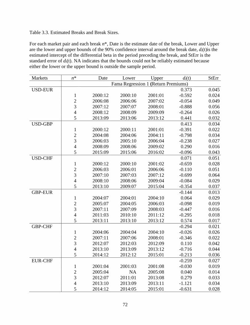
72
Table 3.3. Estimated Breaks and Break Sizes. For each market pair and each break n*, Date is the estimate date of the break, Lower and Upper are the lower and upper bounds of the 90% confidence interval around the break date, di(t)is the estimated intercept of the differential beta in the period preceding the break, and StErr is the standard error of di(t). NA indicates that the bounds could not be reliably estimated because either the lower or the upper bound is outside the sample period. Markets n* Date Lower Upper di(t) StErr Fama Regression 1 (Return Premiums) USD-EUR 0.373 0.045 1 2000:12 2000:10 2001:01 -0.592 0.024 2 2006:08 2006:06 2007:02 -0.054 0.049 3 2007:12 2007:07 2008:01 -0.888 0.056 4 2008:12 2008:09 2009:09 -0.264 0.026 5 2013:09 2013:06 2013:12 0.441 0.032 USD-GBP 0.413 0.034 1 2000:12 2000:11 2001:01 -0.391 0.022 2 2004:08 2004:06 2004:11 -0.798 0.034 3 2006:03 2005:10 2006:04 -0.238 0.027 4 2008:09 2008:06 2009:02 0.290 0.016 5 2015:09 2015:06 2016:02 -0.096 0.043 USD-CHF 0.071 0.051 1 2000:12 2000:10 2001:02 -0.659 0.028 2 2006:03 2006:01 2006:06 -0.110 0.051 3 2007:10 2007:03 2007:12 -0.699 0.064 4 2008:10 2008:06 2009:04 -0.084 0.029 5 2013:10 2009:07 2015:04 -0.354 0.037 GBP-EUR -0.144 0.013 1 2004:07 2004:01 2004:10 0.064 0.029 2 2005:07 2004:05 2006:03 -0.098 0.019 3 2007:11 2007:09 2008:03 -0.447 0.016 4 2011:03 2010:10 2011:12 -0.295 0.018 5 2013:11 2013:10 2013:12 0.574 0.017 GBP-CHF -0.294 0.021 1 2004:06 2004:04 2004:10 -0.026 0.026 2 2007:11 2007:06 2008:01 -0.346 0.022 3 2012:07 2012:03 2012:09 0.110 0.042 4 2013:10 2013:09 2013:12 -0.716 0.044 5 2014:12 2012:12 2015:01 -0.213 0.036 EUR-CHF -0.259 0.027 1 2001:04 2001:03 2001:08 -0.030 0.019 2 2005:04 NA 2005:08 0.040 0.014 3 2012:07 2011:01 2013:08 0.279 0.033 4 2013:10 2013:09 2013:11 -1.121 0.034 5 2014:12 2014:05 2015:01 -0.631 0.028

73
Table 3.3 (cont.) Markets n* Date Lower Upper di(t) StErr Fama Regression 2 (Rate Changes) USD-EUR -0.492 0.039 1 2001:01 2000:10 2001:02 0.480 0.021 2 2006:09 2006:08 2008:01 0.110 0.046 3 2007:11 2007:09 2007:12 0.851 0.050 4 2008:11 2008:09 2009:01 0.250 0.023 5 2013:07 2013:03 2013:09 -0.444 0.028 USD-GBP -0.408 0.031 1 2000:12 2000:11 2001:01 0.338 0.023 2 2003:11 2003:08 2004:01 0.802 0.025 3 2006:04 2005:05 2006:08 0.461 0.025 4 2008:09 2008:05 2009:01 -0.096 0.015 5 2015:09 2015:08 NA 0.199 0.039 USD-CHF -0.088 0.037 1 2000:12 2000:08 2001:02 0.606 0.019 2 2006:08 2006:07 2007:04 0.151 0.043 3 2007:10 2007:07 2007:11 0.659 0.046 4 2008:10 2008:05 2009:01 0.187 0.018 5 2015:09 2015:07 2015:12 0.851 0.046 GBP-EUR -0.108 0.011 1 2005:06 2005:05 2006:01 0.073 0.023 2 2006:09 2006:06 2006:10 -0.149 0.025 3 2007:10 2007:07 2007:11 0.377 0.024 4 2008:12 2008:07 2010:01 0.162 0.012 5 2013:10 2013:08 2013:11 -0.498 0.015 GBP-CHF 0.210 0.024 1 2001:03 2000:10 2001:07 0.038 0.014 2 2006:09 2006:05 2007:03 -0.117 0.031 3 2007:10 2007:06 2007:11 0.285 0.012 4 2014:09 2011:08 NA 0.173 0.032 5 2015:09 2014:08 2015:12 0.570 0.032 EUR-CHF 0.359 0.022 1 2001:03 2001:02 2001:06 0.108 0.014 2 2005:04 2003:06 2005:05 -0.084 0.015 3 2008:12 2008:09 2010:02 0.162 0.013 4 2013:10 2013:09 2013:11 0.779 0.021 5 2015:09 2014:03 2016:01 1.065 0.029

74
Table 3.3 (cont.) Markets n* Date Lower Upper di(t) StErr Fama Regression 3 (Incremental Return Premiums) USD-EUR 0.566 0.062 1 2000:12 2000:10 2001:01 -0.578 0.034 2 2006:03 2006:01 2006:10 0.018 0.062 3 2007:10 2007:05 2007:11 -1.113 0.078 4 2008:10 2008:08 2009:08 -0.361 0.035 5 2013:09 2013:04 2013:10 0.690 0.045 USD-GBP 0.486 0.048 1 2000:12 2000:11 2001:02 -0.423 0.035 2 2003:11 2003:08 2004:03 -0.849 0.040 3 2006:03 2005:04 2006:04 -0.307 0.038 4 2008:09 2008:04 2009:07 0.247 0.023 5 2015:09 2015:06 2016:02 -0.359 0.061 USD-CHF 0.112 0.069 1 2000:12 2000:09 2001:03 -0.821 0.038 2 2006:03 2006:02 2007:02 -0.336 0.069 3 2007:10 2007:01 2007:11 -0.976 0.087 4 2008:10 2008:03 2009:05 -0.274 0.033 5 2015:09 2014:01 2016:08 -0.797 0.087 GBP-EUR 0.002 0.019 1 2003:07 2002:09 2004:09 0.212 0.029 2 2005:04 2003:08 2006:09 0.048 0.024 3 2007:11 2007:10 2008:01 -0.533 0.021 4 2011:03 2010:11 2011:11 -0.343 0.023 5 2013:11 2013:10 2013:12 0.883 0.023 GBP-CHF -0.227 0.023 1 2007:11 2007:08 2009:01 -0.517 0.030 2 2012:10 2012:01 2012:12 -0.145 0.067 3 2013:10 2013:06 2013:12 -0.898 0.062 4 2014:12 2011:08 2015:04 -0.377 0.051 5 EUR-CHF -0.431 0.035 1 2001:03 2001:01 2001:09 -0.137 0.020 2 2006:08 2005:12 2006:10 -0.427 0.047 3 2007:08 2007:01 2007:12 -0.060 0.019 4 2013:10 2013:09 2013:11 -1.652 0.043 5 2014:12 2013:07 2015:01 -1.150 0.035
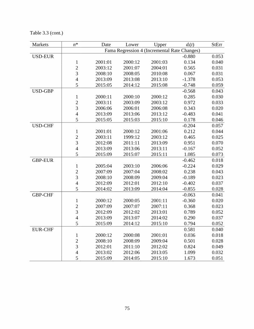
75
Table 3.3 (cont.) Markets n* Date Lower Upper di(t) StErr Fama Regression 4 (Incremental Rate Changes) USD-EUR -0.880 0.053 1 2001:01 2000:12 2001:03 0.134 0.040 2 2003:12 2001:07 2004:01 0.565 0.031 3 2008:10 2008:05 2010:08 0.067 0.031 4 2013:09 2013:08 2013:10 -1.378 0.053 5 2015:05 2014:12 2015:08 -0.748 0.059 USD-GBP -0.568 0.043 1 2000:11 2000:10 2000:12 0.285 0.030 2 2003:11 2003:09 2003:12 0.972 0.033 3 2006:06 2006:01 2006:08 0.343 0.020 4 2013:09 2013:06 2013:12 -0.483 0.041 5 2015:05 2015:03 2015:10 0.178 0.046 USD-CHF -0.204 0.057 1 2001:01 2000:12 2001:06 0.212 0.044 2 2003:11 1999:12 2003:12 0.465 0.025 3 2012:08 2011:11 2013:09 0.951 0.070 4 2013:09 2013:06 2013:11 -0.167 0.052 5 2015:09 2015:07 2015:11 1.085 0.073 GBP-EUR -0.462 0.018 1 2005:04 2003:10 2006:06 -0.224 0.029 2 2007:09 2007:04 2008:02 0.238 0.043 3 2008:10 2008:09 2009:04 -0.189 0.023 4 2012:09 2012:01 2012:10 -0.402 0.037 5 2014:02 2013:09 2014:04 -0.855 0.028 GBP-CHF -0.063 0.041 1 2000:12 2000:05 2001:11 -0.360 0.020 2 2007:09 2007:07 2007:11 0.368 0.023 3 2012:09 2012:02 2013:01 0.789 0.052 4 2013:09 2013:07 2014:02 0.290 0.037 5 2015:09 2014:12 2015:10 0.794 0.052 EUR-CHF 0.581 0.040 1 2000:12 2000:08 2001:01 0.036 0.018 2 2008:10 2008:09 2009:04 0.501 0.028 3 2012:01 2011:10 2012:02 0.824 0.049 4 2013:02 2012:06 2013:05 1.099 0.032 5 2015:09 2014:05 2015:10 1.673 0.051

76
Table 3.4. Univariate Betas and Macroeconomic Conditions. Each panel contains linear regression estimates, where the dependent variables in Panels (a) through (d) are each market’s univariate betas from Fama Regressions 1 through 4, respectively. All independent variables are lagged by one month. Robust standard errors in parentheses. *** p<0.01, ** p<0.05, * p<0.1.
Panel (a): Fama Regression 1 (Return Premiums) EUR GBP CHF USD Credit Spread -0.163 -0.0606 0.0121 -0.288** (0.119) (0.0569) (0.249) (0.129) Policy Rate 0.0358 -0.237*** 0.698*** 0.000533 (0.0720) (0.0399) (0.191) (0.0207) M1 Growth Rate -0.0202* 0.0228*** -0.0316*** 0.00107 (0.0117) (0.00741) (0.00584) (0.00748) Inflation -0.176*** 0.102*** -0.108* -0.220*** (0.0501) (0.0351) (0.0626) (0.0254) Unemployment -0.251*** -0.558*** 0.790*** -0.334*** (0.0534) (0.0459) (0.248) (0.0318) NEER -0.0237** 0.0262*** 0.0413*** -0.0149*** (0.00944) (0.00714) (0.0114) (0.00376) PMI -0.00752 0.0127 -0.0278** 0.0159* (0.00989) (0.00969) (0.0111) (0.00931) VIX -0.0257*** -0.00633** -0.0178 0.0146*** (0.00547) (0.00318) (0.0114) (0.00443) Constant 6.026*** -0.336 -5.668*** 2.888*** (1.365) (0.927) (2.143) (0.969) Observations 140 166 125 191
2R 0.586 0.817 0.336 0.626

77
Table 3.4 (cont.)
Panel (b): Fama Regression 2 (Rate Changes) EUR GBP CHF USD Credit Spread 0.0595 -0.0140 -0.0713 0.383*** (0.0839) (0.0443) (0.182) (0.105) Policy Rate -0.0286 0.203*** -0.431*** -0.00306 (0.0565) (0.0305) (0.130) (0.0191) M1 Growth Rate 0.00353 -0.0224*** 0.0303*** -0.0117* (0.00854) (0.00557) (0.00481) (0.00610) Inflation 0.0558 -0.0890*** 0.129*** 0.191*** (0.0372) (0.0249) (0.0479) (0.0231) Unemployment 0.149*** 0.399*** -0.611*** 0.254*** (0.0435) (0.0341) (0.168) (0.0254) NEER 0.0159** -0.0245*** -0.0301*** 0.0140*** (0.00617) (0.00566) (0.00842) (0.00311) PMI 0.00662 -0.0140* 0.0195** -0.0112 (0.00718) (0.00753) (0.00891) (0.00747) VIX 0.0186*** 0.00920*** 0.0124 -0.0145*** (0.00379) (0.00239) (0.00810) (0.00370) Constant -2.743** 2.032*** 5.112*** -1.612** (1.050) (0.701) (1.534) (0.749) Observations 140 166 125 191
2R 0.549 0.833 0.426 0.574

78
Table 3.4 (cont.)
Panel (c): Fama Regression 3 (Incremental Return Premiums) EUR GBP CHF USD Credit Spread -0.181 -0.0577 0.0741 -0.270 (0.150) (0.0814) (0.322) (0.201) Policy Rate 0.0263 -0.359*** 0.745*** -0.0350 (0.0921) (0.0549) (0.246) (0.0297) M1 Growth Rate -0.0396*** 0.0379*** -0.0476*** -0.00697 (0.0143) (0.0113) (0.00789) (0.0107) Inflation -0.211*** 0.196*** -0.171** -0.294*** (0.0614) (0.0481) (0.0835) (0.0362) Unemployment -0.316*** -0.765*** 0.896*** -0.458*** (0.0698) (0.0610) (0.319) (0.0439) NEER -0.0246** 0.0373*** 0.0408*** -0.0256*** (0.0117) (0.00986) (0.0149) (0.00583) PMI -0.00868 0.0242* -0.0359** 0.0320** (0.0124) (0.0138) (0.0160) (0.0143) VIX -0.0326*** -0.00989** -0.0288** 0.0161*** (0.00677) (0.00437) (0.0132) (0.00610) Constant 7.166*** -0.859 -5.059* 4.187*** (1.713) (1.260) (2.754) (1.556) Observations 140 166 125 191
2R 0.561 0.804 0.349 0.548

79
Table 3.4 (cont.)
Panel (d): Fama Regression 4 (Incremental Rate Changes) EUR GBP CHF USD Credit Spread 0.0758 -0.134* 0.0393 0.393*** (0.110) (0.0681) (0.193) (0.142) Policy Rate -0.128 0.288*** -0.272** 0.0356 (0.0813) (0.0434) (0.128) (0.0252) M1 Growth Rate -0.0143 -0.0407*** 0.0377*** -0.0159** (0.0115) (0.00779) (0.00514) (0.00742) Inflation 0.0409 -0.154*** 0.229*** 0.229*** (0.0436) (0.0334) (0.0542) (0.0336) Unemployment 0.115 0.442*** -0.432*** 0.302*** (0.0694) (0.0455) (0.157) (0.0317) NEER 0.0235*** -0.0357*** -0.0193** 0.0254*** (0.00676) (0.00830) (0.00943) (0.00445) PMI 0.00848 -0.0359*** 0.0231** -0.0256** (0.00994) (0.0106) (0.0101) (0.0104) VIX 0.0277*** 0.0164*** 0.00750 -0.0162*** (0.00457) (0.00343) (0.00886) (0.00467) Constant -3.093** 4.135*** 2.746* -2.666** (1.549) (0.986) (1.600) (1.096) Observations 140 166 125 191
2R 0.611 0.814 0.509 0.450

80
Table 3.5. Results of Principal Component Analysis of the Individual Fama Regressions Betas. We consider both the covariance matrix and correlation matrix when implementing principal component analysis. Only the largest component is reported here. “Standard deviation” is the standard deviation of the component. “Proportion of Variance” is the proportion of variation in the individual betas across the four markets that can be explained by the largest component. “Loadings” are parameters of the linear combination of four betas for constructing the largest component. Regression 1 Regression 2 Regression 3 Regression4
Using Sample Correlation Matrix Standard Deviation 0.984 0.655 1.171 0.800 Proportion of Variance 91.54% 86.17% 93.70% 85.66% Loadings -0.425 -0.283 -0.395 -0.511 -0.451 -0.441 -0.418 -0.383 -0.662 -0.691 -0.715 -0.747 -0.423 -0.498 -0.397 -0.184
Using Sample Covariance Matrix Standard Deviation 1.141 0.817 1.502 0.977 Proportion of Variance 88.88% 82.53% 89.21% 72.26% Loadings -0.354 -0.276 -0.316 0.317 -0.523 -0.551 -0.525 0.557 -0.608 -0.625 -0.604 0.623 -0.481 -0.480 -0.510 0.449

81
Table 3.6. Differential Betas and Macroeconomic Conditions. Each number corresponds to the 2R from a linear regression of the differential betas in the corresponding column on a set of macroeconomic indicators in the corresponding row. The sets of macroeconomic indicators appear as explanatory variables only for the relevant differential betas. All macroeconomic indicators, which include inflation, policy rate, M1 growth rate, unemployment rate, PMI, VIX, credit spread, and NEER, are lagged by one month. USD-EUR USD-GBP USD-CHF GBP-CHF GBP-EUR EUR-CHF
Fama Regression 1 (Return Premiums) Eurozone 0.795
0.664 0.611
UK
0.724
0.251 0.707
Switzerland
0.328 0.179
0.323 US 0.462 0.489 0.372
Fama Regression 2 (Rate Changes) Eurozone 0.874
0.743 0.771
UK
0.691
0.674 0.765
Switzerland
0.316 0.509
0.666 US 0.499 0.417 0.467
Fama Regression 3 (Incremental Return Premiums) Eurozone 0.738
0.633 0.653
UK
0.650
0.305 0.793
Switzerland
0.300 0.134
0.393 US 0.448 0.477 0.322
Fama Regression 4 (Incremental Rate Changes) Eurozone 0.861
0.647 0.732
UK
0.493
0.709 0.675
Switzerland
0.061 0.558
0.747 US 0.463 0.319 0.281

82
Table 3.7. Estimated Number of Breaks and Break Dates for Macroeconomic Indicators. For each macro variable, F(5) is the supremum F-value for the null hypothesis of 5 versus no breaks, Breaks is the estimated number of breaks, Dates are the estimated break dates, BIC(0) is the sample BIC value for the model with no breaks, and BIC(b) is the sample BIC value for the model with the optimal number of breaks. If the F-test indicates no breaks, the BIC is not reported. The smaller the BIC, the better the fit of the model.
Macro Variable F(5) Breaks Dates BIC(0)/ BIC(b)
USD Inflation 95.48 5 2001:09 2004:04 2008:10 2009:10 2014:11 0.59/-0.49 Policy Rate 36.71 5 2000:12 2001:12 2004:05 2007:08 2008:12 -3.19/-3.71 M1 Growth Rate 7.20 0
Unemployment 4.44 0
PMI 6.14 0
VIX 82.07 5 2003:06 2007:07 2008:08 2009:08 2012:01 4.26/3.28 Credit Spread 111.53 5 2001:11 2003:09 2007:07 2008:07 2009:07 -1.58/-2.78 NEER 8.23 0
EUR Inflation 13.98 4 2007:07 2008:07 2009:07 2011:04 -2.79/-2.96 Policy Rate 20.35 4 2000:10 2003:06 2008:07 2009:07 -3.76/-4.05 M1 Growth Rate 13.54 5 2001:03 2003:03 2008:08 2009:08 2011:05 -0.47/-0.63 Unemployment 6.83 0
PMI 21.00 3 2008:02 2009:02 2010:04 0.48/0.23 VIX 67.34 5 2002:05 2003:05 2008:08 2009:08 2012:08 4.39/3.54 Credit Spread 111.53 5 2001:11 2003:09 2007:07 2008:07 2009:07 -1.58/-2.78 NEER 5.30 0
GBP Inflation 12.85 5 2007:09 2008:09 2009:09 2011:09 2012:09 -2.51/-2.65 Policy Rate 23.34 4 2000:11 2001:11 2008:03 2009:03 -3.50/-3.84 M1 Growth Rate 76.81 5 2001:12 2003:12 2008:12 2012:05 2013:05 3.08/2.14 Unemployment 12.89 4 2000:06 2003:03 2008:03 2009:03 -3.85/-4.00 PMI 4.09 0
VIX 57.35 5 2002:05 2003:05 2007:06 2008:08 2009:08 4.13/3.36 Credit Spread 111.53 5 2001:11 2003:09 2007:07 2008:07 2009:07 -1.58/-2.78 NEER 9.08 3 2007:08 2009:01 2015:08 1.12/1.02
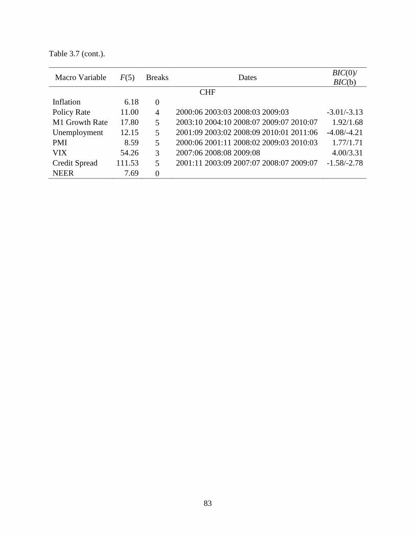
83
Table 3.7 (cont.).
Macro Variable F(5) Breaks Dates BIC(0)/ BIC(b)
CHF Inflation 6.18 0
Policy Rate 11.00 4 2000:06 2003:03 2008:03 2009:03 -3.01/-3.13 M1 Growth Rate 17.80 5 2003:10 2004:10 2008:07 2009:07 2010:07 1.92/1.68 Unemployment 12.15 5 2001:09 2003:02 2008:09 2010:01 2011:06 -4.08/-4.21 PMI 8.59 5 2000:06 2001:11 2008:02 2009:03 2010:03 1.77/1.71 VIX 54.26 3 2007:06 2008:08 2009:08 4.00/3.31 Credit Spread 111.53 5 2001:11 2003:09 2007:07 2008:07 2009:07 -1.58/-2.78 NEER 7.69 0

84
Figure 3.1. Estimated One Month Spot Rates.

85
Figure 3.2. Slope Coefficients and Two Standard Deviation Confidence Intervals: Fama Regression 1 (Return Premiums).
Panel (a): USD Panel (b): EUR
Panel (c): GBP Panel (d): CHF

86
Figure 3.3. Slope Coefficients and Two Standard Deviation Confidence Intervals: Fama Regression 2 (Rate Changes).
Panel (a): USD Panel (b): EUR
Panel (c): GBP Panel (d): CHF
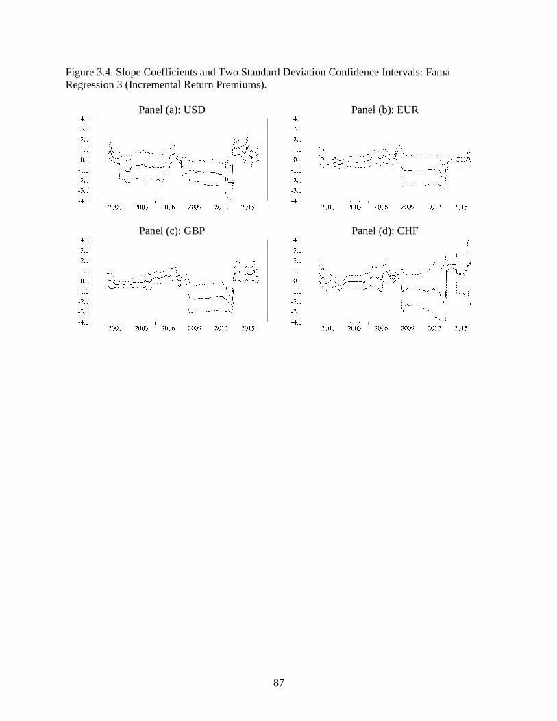
87
Figure 3.4. Slope Coefficients and Two Standard Deviation Confidence Intervals: Fama Regression 3 (Incremental Return Premiums).
Panel (a): USD Panel (b): EUR
Panel (c): GBP Panel (d): CHF

88
Figure 3.5. Slope Coefficients and Two Standard Deviation Confidence Intervals: Fama Regression 4 (Incremental Rate Changes).
Panel (a): USD Panel (b): EUR
Panel (c): GBP Panel (d): CHF

89
Figure 3.6. Differential Betas and Two Standard Deviation Confidence Intervals: Fama Regression 1 (Return Premiums).
Panel (a): USD-EUR Panel (b): USD-GBP
Panel (c): USD-CHF Panel (d): GBP-EUR
Panel (e): GBP-CHF Panel (f): EUR-CHF
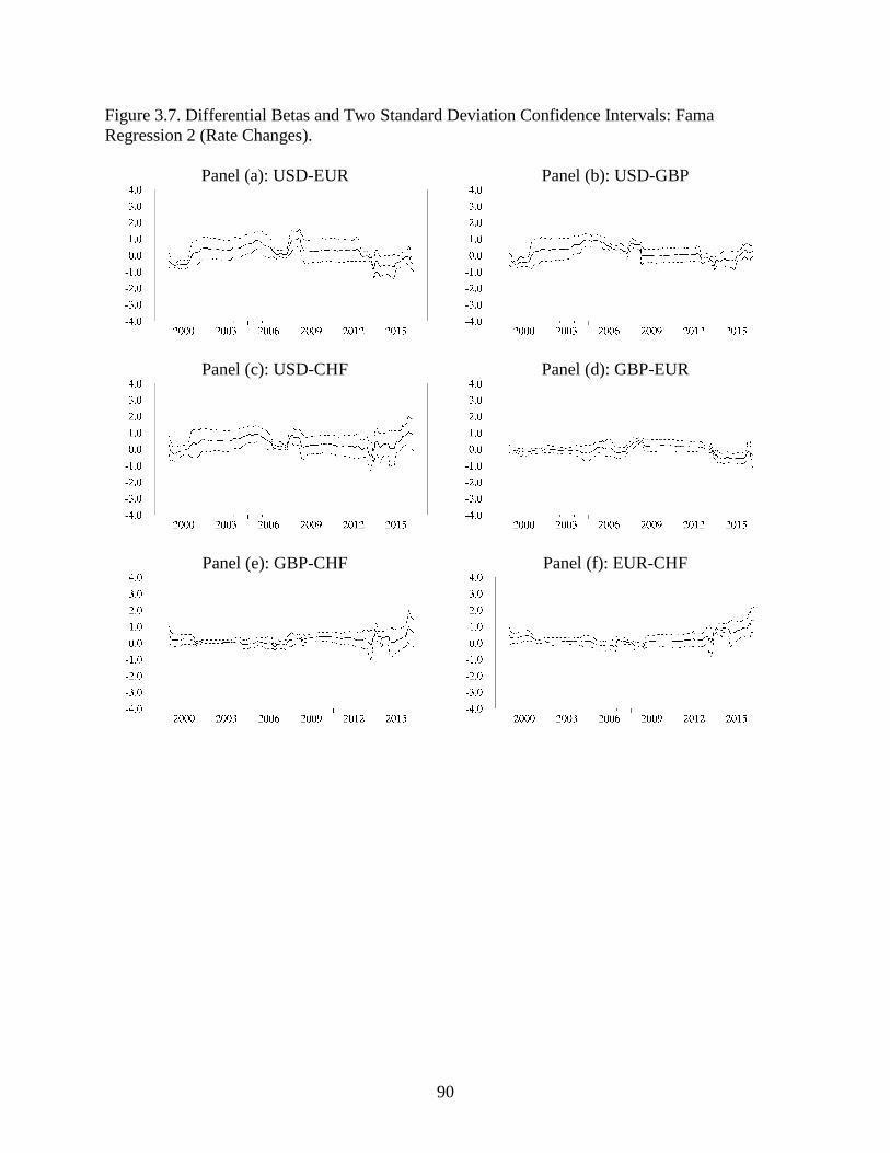
90
Figure 3.7. Differential Betas and Two Standard Deviation Confidence Intervals: Fama Regression 2 (Rate Changes).
Panel (a): USD-EUR Panel (b): USD-GBP
Panel (c): USD-CHF Panel (d): GBP-EUR
Panel (e): GBP-CHF Panel (f): EUR-CHF

91
Figure 3.8. Differential Betas and Two Standard Deviation Confidence Intervals: Fama Regression 3 (Incremental Return Premiums).
Panel (a): USD-EUR Panel (b): USD-GBP
Panel (c): USD-CHF Panel (d): GBP-EUR
Panel (e): GBP-CHF Panel (f): EUR-CHF

92
Figure 3.9. Differential Betas and Two Standard Deviation Confidence Intervals: Fama Regression 4 (Incremental Rate Changes).
Panel (a): USD-EUR Panel (b): USD-GBP
Panel (c): USD-CHF Panel (d): GBP-EUR
Panel (e): GBP-CHF Panel (f): EUR-CHF

93
Figure 3.10. Time-Varying Correlations: Fama Regression 1 (Return Premiums).
Panel (a): USD-EUR Panel (b): USD-GBP
Panel (c): USD-CHF Panel (d): GBP-EUR
Panel (e): GBP-CHF Panel (f): EUR-CHF
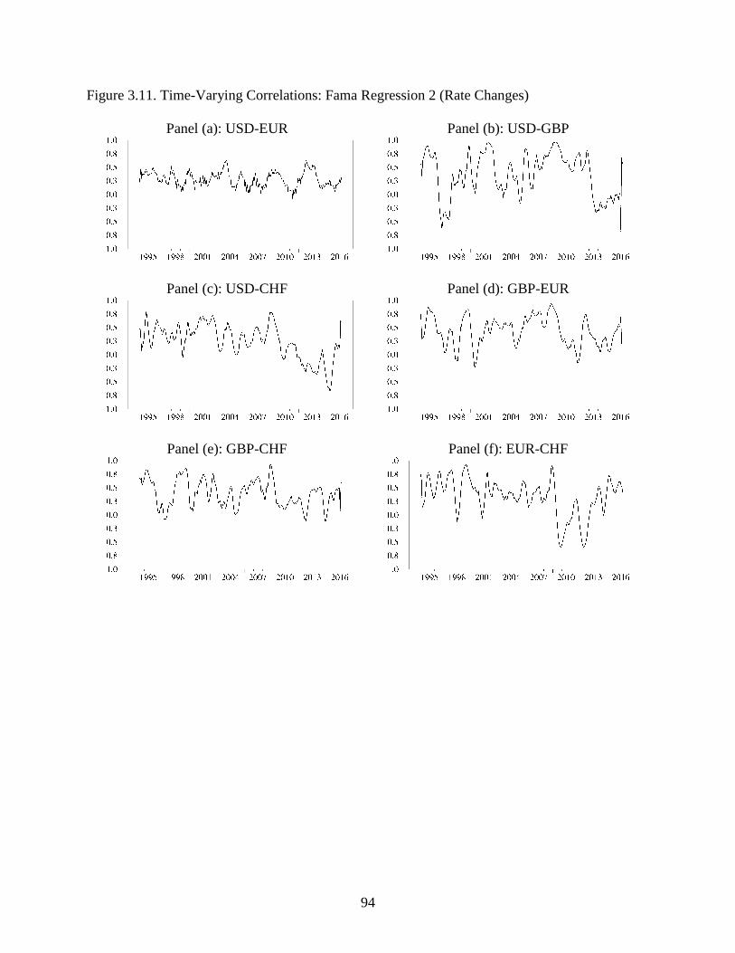
94
Figure 3.11. Time-Varying Correlations: Fama Regression 2 (Rate Changes)
Panel (a): USD-EUR Panel (b): USD-GBP
Panel (c): USD-CHF Panel (d): GBP-EUR
Panel (e): GBP-CHF Panel (f): EUR-CHF

95
Figure 3.12. Time-Varying Correlations: Fama Regression 3 (Incremental Return Premiums).
Panel (a): USD-EUR Panel (b): USD-GBP
Panel (c): USD-CHF Panel (d): GBP-EUR
Panel (e): GBP-CHF Panel (f): EUR-CHF
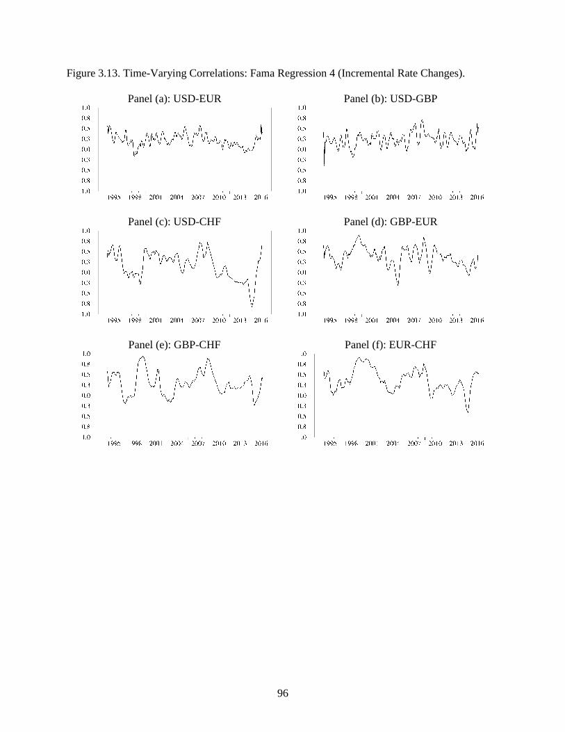
96
Figure 3.13. Time-Varying Correlations: Fama Regression 4 (Incremental Rate Changes).
Panel (a): USD-EUR Panel (b): USD-GBP
Panel (c): USD-CHF Panel (d): GBP-EUR
Panel (e): GBP-CHF Panel (f): EUR-CHF

97
Figure 3.14. Results of Principal Component Analysis of the Individual Fama Regression Betas.

98
CHAPTER 4: SAMUELSON HYPOTHESIS, ARBITRAGE ACTIVITY, AND FUTURES RISK PREMIUMS
4.1. Introduction
The prediction that futures volatility increases as the expiration date approaches has
become known as the Samuelson hypothesis after Samuelson (1965) used it as an illustration of
his theoretical model. The inverse relationship between futures volatility and time to maturity is
also referred to as simply the maturity effect in some of the literature.
Studying futures volatility term structure is important for several reasons. First, the term
structure of volatility influences the selection of the number of futures contracts and the specific
contract used for hedging in a futures-based hedging strategy. Second, the volatility term
structure determines the value of futures options, related derivatives, and the corresponding
implied risk parameters. Third, a better understanding of the futures volatility term structure can
improve the process of setting futures margin requirements, leading to a safer and more efficient
trading environment. Fourth, the volatility term structure affects the equilibrium risk premium in
futures markets (Hirshleifer, 1988) and, therefore, the cost of hedging.
Our focus is on the slope of the futures volatility term structure. The negative slope of the
futures volatility term structure is often interpreted as an implication of the hypothesis that
futures volatility increases as the time to maturity nears. Our approach is to capture the
information in the volatility term structure with three factors that are related to the level, slope,
and curvature of the term structure. This design allows us to study the evolution of the
Samuelson hypothesis in each market over time because the three factors can be seen as driving

99
the dynamics of the volatility term structure, so that time-series variation in the slope
factor is a measure of the time-series variation in the strength of the maturity effect. In addition,
our design allows us to directly relate the slope of the volatility term structure to the level of
inventories and to the futures term premiums.
We study the volatility term structure in ten futures markets comprising three categories:
agriculture, energy, and metals. We show that there is significant time-series variation in the
strength of the maturity effect in each market. We also show that the slope of the volatility term
structure is more negative when inventories are low and that the threshold for high/low inventory
is specific to each market. Our explanation of the relationship between the Samuelson hypothesis
and inventory levels is rooted in the cost-of-carry model. The empirically observed threshold
behavior is indicative of carry arbitrage being feasible only when inventories are sufficiently
high. Our hypothesis that presence of carry arbitrage is the driving force behind the absence of
the maturity effect is further corroborated by tests showing that futures term premiums vanish
when the slope factor approaches zero.
Existing literature on the Samuelson hypothesis can largely be subdivided into mostly
theoretical and mostly empirical with a few exceptions (Bessembinder, Coughenour, Seguin, &
Smoller, 1996; Brooks, 2012) that contribute both theoretically and empirically. Theoretical
papers focus on establishing a set of conditions that lead to the existence of the maturity effect in
futures markets.
Rutledge (1976) shows that the maturity effect is supported by the Samuelson’s model
only when the spot price follows a stationary autoregressive process and does not hold when the
spot price process is random walk. Anderson and Danthine (1983) introduce a multi-period
model of hedging in which futures prices are volatile in times when much uncertainty is resolved

100
and are stable when little uncertainty is resolved; the maturity effect can then be interpreted as a
special case of the Anderson-Danthine state-variable framework whereby progressively more
information is revealed as the maturity date approaches. Bessembinder et al. (1996) establish a
framework that identifies the conditions under which the Samuelson hypothesis is expected to
hold; specifically, they show that the hypothesis will generally be supported in markets where
the spot prices and convenience yields are positively correlated, whereas clustering of
information near the delivery dates is not a necessary condition for the hypothesis to hold.
Routledge, Seppi, and Spatt (2000) introduce a model of joint dynamics of spot prices
and inventories and prove that within their model the Samuelson hypothesis need not hold
conditionally. Specifically, they show that when inventory is sufficiently high it is possible for
the opposite of the Samuelson hypothesis to hold: forward price volatility is an increasing
function of time to maturity. Brooks (2012) develops a futures market representation showing
that the Samuelson hypothesis cannot hold in fully arbitraged markets; moreover, the inverse link
between the hypothesis and carry arbitrage appears to be continuous in the sense that the
maturity effect is stronger (weaker) when carry arbitrage forces are weaker (stronger).
Because the Samuelson hypothesis is an empirical proposition, there is a large empirical
literature. Most studies that test the hypothesis across a variety of markets find mixed results.
Rutledge (1976) finds support for the hypothesis in silver and cocoa futures, but not in wheat and
soybean futures. Castelino and Francis (1982) study the volatility of changes in the basis and find
support for the Samuelson hypothesis in wheat, soybeans, soybean oil, and soybean meal futures.
Anderson (1985) finds that various forms of seasonality are a stronger determinant of
futures volatility than the maturity effect; nonetheless, the maturity effect is still present in oats,
soybean oil, live cattle, and cocoa futures, while it is absent in wheat, corn, soybeans, and silver

101
futures. Milonas (1986) extends the work of Anderson and shows that the maturity effect is
present in 10 out of 11 markets (not present in corn futures), including Treasury bond futures and
industrial and precious metals, even after accounting for the contract month effect.
Barnhill, Jordan, and Seale (1987) control for the effect of quarterly refunding on the
volatility of Treasure bond futures and still find support for the Samuelson hypothesis, which is
stronger of the two effects. Kenyon et al. (1987) identify and control for several economic
factors that affect futures volatility from year to year and still reach the conclusion that the
maturity effect is present in corn, soybeans, and wheat futures. Khoury and Yourougou (1993)
provide international evidence in support of the maturity effect by showing that six agricultural
commodity futures traded on the Winnipeg exchange are driven by the same five determinants
(month and year seasonality, trading session effect, contract month effect, and maturity effect)
that drive the corresponding U.S. futures markets.
Based on the theory of storage (Working, 1949; Brennan, 1958; Telser, 1958), Fama and
French (1988) predict that the maturity effect should (not) hold when inventories are low (high)
and, using a proxy for inventory levels, find empirical support for this refinement of the
Samuelson hypothesis in the futures markets for industrial metals. In the most extensive study of
the Samuelson hypothesis at the time of publication, Galloway and Kolb (1996) study the term
structure of volatility in 45 markets, including agricultural and energy commodity futures,
precious and industrial metal futures, and stock index, currency, and interest rate futures. Their
findings provide support for the maturity effect in agricultural and energy commodities, but not
in precious metals and financials. Galloway and Kolb conclude that the maturity effect is present
in commodities that exhibit seasonal supply and demand patterns, but is virtually nonexistent in
the markets where the cost-of-carry model works well.

102
Bessembinder et al. (1996) find that the Samuelson effect holds in agricultural and crude
oil futures and less strongly in metal futures, while it does not hold in financial futures. Their
conclusion is that empirical evidence is consistent with their prediction that the presence of a
mean reverting component in the spot price process (negative correlation between the spot price
and the slope of the futures price term structure) governs the presence of the maturity effect.
Duong and Kalev (2008) use intraday data from 20 futures markets to construct a
measure of futures volatility as a sum of squared intraday returns and find that the Samuelson
hypothesis holds in agricultures futures, but does not hold in other futures. They also show that
their findings are consistent with the negative covariance explanation of Bessembinder et al.
(1996). Kalev and Duong (2008) also use intraday data, but measure futures volatility as the
realized intraday range and find that among 14 futures markets there is strong support for the
Samuelson hypothesis in agricultural futures and no support in any of metal and financial
futures.
Gurrola & Herrerías (2011) study the maturity effect in the Mexican interest rate futures
using panel data techniques and find that the inverse of the Samuelson hypothesis prevails:
volatility increases with time to expiration. To reconcile the findings with the negative
covariance theory of Bessembinder et al. (1996), the study describes additional criteria that must
be met in order for the maturity effect to hold. Liu (2016) uses stochastic volatility as a measure
of futures volatility and examines the maturity effect using stochastic dominance tests. While
there is mild support for the Samuelson hypothesis in energy futures in terms of the first two
degrees of stochastic dominance, the hypothesis is more likely to hold at low stochastic volatility
levels. Jaeck and Lautier (2016) find support for the Samuelson hypothesis in electricity markets

103
and show that shocks propagate from the spot to the futures contracts with intensity decreasing
as time to expiration increases.
We contribute to the literature on the futures markets and specifically their volatility term
structure in several ways. First, we point out a common technical issue that plagues time-series
studies of futures prices and propose a method of overcoming it with a well-known interpolation.
A common approach is to construct time-series of futures prices on a nearby basis; however, the
time to expiration varies even within a given nearby time-series, introducing noise into the
volatility-maturity relationship. We overcome the maturity drift problem by interpolating futures
prices with a Nelson and Siegel (1987) curve and then using a point on the curve corresponding
to an exact maturity. The result is a vector of futures price time-series with each time-series
corresponding to an exact maturity on every trading day.
Second, borrowing from the literature on modeling the term structure of interest rates, we
impose a factor model on the futures volatility term structure to parsimoniously explain the
changes in the shape of term structure as being driven by just three factors. We fit the Nelson and
Siegel model to the observed volatility term structure and, following Diebold and Li (2006),
interpret model estimates as dynamic factors whose time-series behavior determines changes in
the shape of the volatility term structure. This interpretation allows us to study the time-series
variation in the strength of the Samuelson effect as represented by the variation in the slope
factor. We show that in most markets the slope factor is strongly negative in certain periods and
only weakly or not at all negative in other periods, reflecting varying strength of the Samuelson
effect.
Third, we provide new evidence in support of the ability to conduct carry arbitrage as the
driving force behind the Samuelson effect. We first show that the maturity effect is weaker when

104
inventories are high, which could be consistent with several explanations of the Samuelson
effect. Specifically, we find that high inventory levels correspond to a flatter volatility term
structure in corn, wheat, crude oil, heating oil, gold, silver, and copper futures. We next show
that the link between inventories and the maturity effect exhibits threshold behavior, which can
be consistent with the carry arbitrage explanation, but not with other theories put forth to explain
the Samuelson effect.
Fourth, we study the link between the Samuelson hypothesis and futures risk premiums.
When the volatility term structure flattens, term premiums in all futures markets except for wheat
move closer to zero, consistent with the explanation that arbitrageurs provide infinite supply to
meet net hedging demand.
4.2. Data
We examine the most actively traded physical commodity futures in three broad
categories: agriculture, energy, and metals.35 The agriculture category includes corn futures
(ticker: C), soybean futures (S), and Chicago soft red winter wheat futures (W). The energy
category is comprised of crude oil futures (CL), heating oil futures (HO),36 Henry Hub natural
gas futures (NG), and reformulated blend futures (RB).37 Copper futures (HG), gold futures
(GC), and silver futures (SI) are the contracts in the metals category.
Using daily data from 6/1/1993 to 2/28/2017, we form time-series of futures prices, time
to maturity, and open interest for up to twelve futures contracts nearest to expiration for each
commodity. We follow the standard practice in the literature and construct a vector of continuous
35 We only consider futures traded on U.S. exchanges, namely CME, COMEX, and NYMEX. In each of the three categories we select three to four most actively traded contracts based on open interest. See http://www.cmegroup.com/education/files/cme-group-leading-products-2017-q2.pdf. 36 The contract currently traded under the HO ticker is the New York Harbor Ultra-Low Sulfur Diesel futures. 37 The full contract name is RBOB (reformulated blendstock for oxygenated blending) gasoline futures.

105
series ordered based on closeness to expiration, from the nearest to the most distant. We choose
the last day of trading of the expiring contract as the rollover date since no significant difference
has been found between different choices of the rollover date (Carchano and Pardo, 2009).
The resulting time-series are ordered by maturity in the sense that on any given trading
day the first nearby contract is closer to expiration than the second nearby and so forth; however,
even within a given series there is a day to day variation in the time to maturity because the
contracts whose prices are used in constructing the series gradually expire and are replaced by
new contracts. For example, the first nearby contract in any of the energy futures ranges in
maturity from 23 days to 1 day. To address the maturity drift problem that could introduce noise
in the volatility-maturity relationship, we fit a Nelson and Siegel (1987) curve to the observed
daily term structure of futures prices and then obtain predicted values (pseudo prices) that
correspond to exact maturities of 1 through 12 months.38 Because our goal is to simply
interpolate the futures price term structure, we follow the original interpretation of the Nelson
and Siegel model as an approximating function that can be used to interpolate and extrapolate
data that exhibits exponential decay and curvature in the maturity dimension; we do not attempt
to interpret the price term structure as determined by the factors derived from the Nelson and
Siegel model (we do this for the volatility term structure).
Because our interest is in the term structure of volatility of commodity futures, we
aggregate the daily data into a monthly frequency to obtain an estimate of the futures volatility in
any given month. This estimate is simply the annualized standard deviation of daily changes in
the logarithm of the futures prices during the month in question. As a result of aggregation, we
have a sample of 285 observations of futures volatility, as well as intra-month averages of futures
38 The pseudo prices can be viewed as daily-rebalanced weighted average of the prices of two actual futures contracts.

106
returns and open interest. With pseudo prices time to maturity is fixed for each daily observation,
but with raw prices we must use the average time to maturity within the month as corresponding
to that month’s futures volatility.
The inventory data for the underlying commodities is from Bloomberg, where it is
compiled from original sources. The original source of the inventory data for agricultural
commodities is the USDA World Agricultural Supply and Demand Report. The report contains
monthly data on U.S. total ending stocks of corn, soybeans, and wheat. The energy inventory
data originates from the Energy Information Administration (EIA). The EIA reports weekly
ending stocks for various hydrocarbons. Inventory data for precious and industrial metals
originates from COMEX and NYMEX. These inventories are reported on the daily basis and
represent the stocks at depositories and warehouses designated for delivery under the contracts.
As a measure of crude oil inventory, we use U.S. ending stocks of crude oil excluding
Strategic Petroleum Reserve. Because the underlying commodity for heating oil futures is ultra-
low sulfur diesel, we use U.S. ending stocks of distillate fuel oil (containing 15 part per million
sulfur or less) as our measure of heating oil inventory. U.S. natural gas inventories held in
underground storage facilities serve as our measure of natural gas inventory. Reformulated blend
futures specify that the underlying is reformulated regular gasoline blendstock for blending with
10% denatured fuel ethanol, but beginning in 2010 the EIA reports only the total stocks of
reformulated gasoline blendstock for oxygenated blending (with either ethanol or ethers).
Therefore, we use ending stocks of reformulated blendstock for oxygenated blending as our
measure of reformulated blend inventory, without distinguishing blendstock intended for mixing
with ethanol from blendstock intended for mixing with ethers.
107
Futures open interest represents the number of outstanding contracts, so we convert
inventory numbers from the physical units into the hypothetical number of contracts that could
be fulfilled with the available inventory, thereby facilitating comparisons with open interest.
Table 4.1 reports summary statistics for each commodity. The numbers are the exact
times to expiration (measured in months) and the sample means of open interest, inventories, and
futures return volatility. We also report the autoregressive coefficient from an AR(1) model of
volatility dynamics as a measure of volatility persistence. Each column corresponds to the index
of the futures contract, starting with contract nearest to expiration (1) and ending with the
contract most distant from expiration (12). In the last column, we report the total open interest
across the twelve contracts, the inventories, and the ratio of inventories to total open interest.
The more distant contracts are not always traded actively. The second nearby is generally
the most actively traded contract in all commodities except for crude oil.39 In the agriculture
category, open interest in the fifth through seventh nearby contract is roughly one tenth of open
interest in the second nearby and much less in the more distant contracts. In the energy category
(except for reformulated blend), the more distant contracts are still actively traded with even the
tenth to twelfth nearby futures having more than one tenth of the open interest in the second
nearby contract. Trading in the fourth through seventh nearby contracts in the metals category
generates roughly one tenth of the open interest in the second nearby with the more distant
futures trading even less actively.
39 Because the commodity futures contracts are physical settled, the hedgers must unwind their positions in the nearest contract to avoid having to take delivery under the contract, which depresses open interest in the first nearby contract in those commodities where trading is still possible during the delivery month (trading in crude oil futures ceases the month before the delivery month, so that hedgers do not need to unwind their positions until the last day of trading).

108
The Samuelson effect is particularly pronounced in the agriculture and energy category
futures, where futures volatility declines monotonically in almost all cases as the time to
expiration increases. The difference in volatility between the nearest and the most distant futures
is seven to eight percentage points for corn and soybeans; 10 to 12 percentage points for wheat,
crude oil, and heating oil; 14 percentage points for reformulated blend; a staggering 28
percentage points for natural gas. In the metals category, the Samuelson effect is weak in copper
futures and nonexistent in gold and silver futures. A flat average term structure in the metals
futures and the monotonically declining average term structure in the energy and agricultural
futures are consistent with the findings in Brooks (2012). Long-term volatilities are not only
lower than the short-term volatilities, they are also more persistent. Important exceptions are the
gold and silver futures markets, where the persistence of volatility does not seem to increase with
maturity – another observation consistent with Brooks (2012).
Sample means of the futures return volatilities coupled with the exact futures maturities
can be thought of as the sample average term structure of volatility. Figure 4.1 contains plots of
the average volatility term structure for each commodity. The plots reveal that not only do the
volatility term structures of agricultural and energy futures slope downward, but that they are
also convex. This convexity is strongest in energy futures, while agricultural futures seem to
have a more linear volatility term structure at longer maturities.
4.3. Estimation of the Volatility Term Structure
The main prediction of the Samuelson hypothesis is that the volatility term structure is
downward sloping. One way to empirically measure the slope of the term structure is to take the
difference between the volatility of the most distant futures contract and the contract nearest to
expiration. However, this approach ignores the information contained in the volatility of the
109
intermediate contracts. Therefore, to capture this information we estimate the slope of the
volatility term structure by fitting a curve to the observed volatilities of contracts with different
maturities. The slope of this curve can be thought of as a measure of the slope of the volatility
term structure.
To estimate the slope of the volatility term structure we use the Nelson and Siegel (1987)
functional form, which is a three factor approximation that imposes an exponential structure on
the factor loadings. Christensen, Diebold, and Rudebusch (2009) note that the Nelson and Siegel
framework fits the cross-section of bond yields in many countries remarkably well and has been
widely used by financial market participants and central banks. Diebold and Li (2006) estimate
the Nelson and Siegel yield curve period by period and show that the three time-varying
parameters of the model can be interpreted as factors corresponding to level, slope, and
curvature, and that their time-series behavior can be efficiently estimated with autoregressive
models. The alternative to the Diebold and Li approach is to cast the model in a state-space
representation with latent factor loadings taking the Nelson and Siegel exponential form
(Diebold, Li, and Yue, 2008).
We follow Diebold and Li (2006) and fit the time-series of futures volatility term
structures period by period rather than cast the model in a state-space representation. We use the
following factorization of the Nelson and Siegel model:
𝜎𝜎𝑡𝑡(𝜏𝜏) = 𝛽𝛽1𝑡𝑡 + 𝛽𝛽2𝑡𝑡 �1 − 𝑣𝑣−𝜆𝜆𝑡𝑡𝜏𝜏
𝜆𝜆𝑡𝑡𝜏𝜏� + 𝛽𝛽3𝑡𝑡 �
1 − 𝑣𝑣−𝜆𝜆𝑡𝑡𝜏𝜏
𝜆𝜆𝑡𝑡𝜏𝜏− 𝑣𝑣𝑒𝑒−𝜆𝜆𝑡𝑡𝜏𝜏� (4.1)
where 𝜎𝜎𝑡𝑡(𝜏𝜏) is the time 𝑡𝑡 volatility of the futures contract with maturity 𝜏𝜏 (measured in months),
and 𝜃𝜃𝑡𝑡 = {𝛽𝛽1𝑡𝑡,𝛽𝛽2𝑡𝑡,𝛽𝛽3𝑡𝑡, 𝜆𝜆𝑡𝑡} are estimated parameters that govern the shape of the volatility term
structure. We can interpret 𝛽𝛽1𝑡𝑡 as the factor that governs the level of the volatility term structure
because lim𝜏𝜏→∞
𝜎𝜎𝑡𝑡(𝜏𝜏) = 𝛽𝛽1𝑡𝑡. If we define the slope of the volatility term structure as 𝜎𝜎𝑡𝑡(∞) −

110
𝜎𝜎𝑡𝑡(0), then 𝛽𝛽2𝑡𝑡 can be interpreted as the factor that governs the slope of the volatility term
structure because lim𝜏𝜏→∞
𝜎𝜎𝑡𝑡(𝜏𝜏) − lim𝜏𝜏→0
𝜎𝜎𝑡𝑡(𝜏𝜏) = −𝛽𝛽2𝑡𝑡. Even if we define the slope as 𝜎𝜎𝑡𝑡(12) − 𝜎𝜎𝑡𝑡(0),
then −𝛽𝛽2𝑡𝑡 is still closely related to the slope of the volatility term structure because40 𝜎𝜎𝑡𝑡(12) −
lim𝜏𝜏→0
𝜎𝜎𝑡𝑡(𝜏𝜏) = −0.977𝛽𝛽2𝑡𝑡 + 0.023𝛽𝛽3𝑡𝑡. Lastly, 𝛽𝛽3𝑡𝑡 can be interpreted as the factor that governs the
curvature of the term structure because an increase in 𝛽𝛽3𝑡𝑡 will most significantly affect medium-
term volatilities, but have little effect on the short-term and long-term volatilities, leading to an
increase in the curvature of the term structure. Because of our interpretation, we refer to 𝛽𝛽1𝑡𝑡,
−𝛽𝛽2𝑡𝑡, and 𝛽𝛽3𝑡𝑡 as the level, slope, and curvature factors.
The parameter 𝜆𝜆𝑡𝑡 governs the exponential decay rate and controls where the loading on
𝛽𝛽3𝑡𝑡 achieves its maximum. We could estimate the parameters 𝜃𝜃𝑡𝑡 = {𝛽𝛽1𝑡𝑡,𝛽𝛽2𝑡𝑡,𝛽𝛽3𝑡𝑡,𝜆𝜆𝑡𝑡} by
nonlinear least squares, but instead we fix 𝜆𝜆𝑡𝑡 at a prespecified value, which allows us to first
calculate factor loadings and then estimate the models using ordinary least squares. We set the
value 𝜆𝜆𝑡𝑡 = 3.58656 to maximize the loading on the curvature factor at the six-month maturity.
Because prior literature has not examined where the volatility term structure of commodity
futures tends to achieve its maximum curvature, we choose the maturity corresponding to the
maximum curvature based on the plots in Figure 4.1.41
While the Nelson and Siegel framework has been predominantly applied to the term
structure of interest rates, we expect it to also be a good model of the dynamics of futures
volatility term structure. Although it is ultimately an empirical matter, the model has the ability,
in principle, to capture the following stylized facts about the volatility term structure:
40 Setting 𝜆𝜆𝑡𝑡 = 3.58656 for reasons outlined below. 41 We examine several different values of 𝜆𝜆𝑡𝑡 that maximize volatility term structure curvature anywhere between four and eight months and obtain quantitatively similar results in subsequent tests.

111
(1) The average volatility term structure is decreasing and convex. In the Nelson and Siegel
framework, the average volatility terms structure corresponds to the average values of 𝛽𝛽1𝑡𝑡,
𝛽𝛽2𝑡𝑡, and 𝛽𝛽3𝑡𝑡, and the functional form guarantees that the fitted curve can assume a decreasing
and convex shape.
(2) Depending on the commodity and the time period, the volatility term structures can assume a
variety of shapes, including downward sloping, upward sloping, humped, and inverted
humped. The Nelson and Siegel curve can assume any of these shapes and the frequency
with which it changes the shapes depends entirely on the behavior of 𝛽𝛽1𝑡𝑡, 𝛽𝛽2𝑡𝑡, and 𝛽𝛽3𝑡𝑡.
(3) Volatility dynamics are persistent, but the volatility spreads are somewhat less persistent.42
Strong persistence of volatility dynamics can be explained by high persistence of 𝛽𝛽1𝑡𝑡, and a
weaker persistence of volatility spreads can be explained by lower persistence of 𝛽𝛽2𝑡𝑡.
(4) Long-term volatilities are more persistent than the short-term volatilities. In the Nelson and
Siegel framework, the long-term volatilities depend only 𝛽𝛽1𝑡𝑡, so if 𝛽𝛽1𝑡𝑡 is the most persistent
factor, then long-term volatilities will be more persistent than short-term.
We estimate the model in equation (4.1) for every month 𝑡𝑡 by regressing futures return
volatility on the factor loadings. Table 4.2 reports the sample mean, standard deviation, and the
AR(1) coefficient (measure of persistence) of the level factor, the slope factor, and the empirical
slope of term structure, which we calculate as 𝜎𝜎𝑡𝑡(12) − 𝜎𝜎𝑡𝑡(1). We also report the correlation
coefficient between the estimated slope factor and the empirical slope of the term structure. The
last column of the table reports the sample mean of the 2R as a measure of fit of the Nelson and
Siegel model to the observed volatility term structure.
42 Table 2 reports the autoregressive coefficient from an AR(1) model as a measure of persistence of volatility spread (see the Empirical Slope AR(1) column).

112
The statistics in Table 4.2 allow us to draw conclusions about the empirical validity of the
Nelson and Siegel framework as an approximation of the futures volatility term structure. We
find that the model’s principal ability to fit a variety of possible shapes of the term structure
translates into high average 𝑅𝑅2 across most commodities. The level factor is generally more
persistent than the slope factor (the two have similar persistence in heating oil, natural gas, and
reformulated blend futures), explaining higher persistence of observed volatilities and lower
persistence of volatility spreads. In addition, the level factor is significantly more persistent than
the curvature factor43, so that it is generally the most persistent of the three factors, which is
consistent with our observation that long-term volatilities are generally more persistent than the
short-term volatilities.
There are two other important observation to be made regarding Table 4.2. First, the
standard deviation of the slope factor is appreciably higher than the standard deviation of the
empirical slope in seven of the ten commodities, while in the other three commodities the
standard deviations are almost equal. The slope factor experiences higher variability because it
incorporates the information from the entire term structure rather than just two points. The
incorporation of information is the theoretical reason why we work with the estimated slope
factor instead of the empirical slope, but from a practical point of view the higher time-series
variation of the slope factor can also help with identification. Second, in most commodities the
slope factor is moderately persistent, which justifies our methodological choice of calculating
futures volatility over disjoint monthly intervals rather than using rolling calculations or GARCH
models, both of which would yield a larger sample, but introduce additional autocorrelations to
an already persistent series.
43 The AR(1) coefficients of the curvature factor range from 0.008 for silver to 0.385 for reformulated blend.

113
4.4. Results
The Nelson and Siegel estimates of the futures volatility term structure allow us to
parsimoniously study the time-series evolution of the Samuelson effect in each of the futures
markets. On the one hand, the summary statistics of the return volatility of futures contracts with
various maturities indicate that the Samuelson effect was present (in terms of economic
significance), on average, in all but two markets – gold and silver. The Nelson and Siegel
estimates of the slope factor tell a similar story – the sample mean of the factor is reliably
negative in the agriculture and energy categories, less negative in the copper market, and very
close to zero in the gold and silver markets (based on economic significance; statistically, they
are all significantly negative at the 1% level). On the other hand, we cannot rule out the
possibility that there were periods of time when the Samuelson effect was weaker or stronger in
each of the markets.
In order to study the time-series variation in the strength of the Samuelson effect, we
construct the 60-month moving average of the slope factor and the corresponding 95%
confidence bands.44 We use the 60-month window because it is small enough to readily capture
any shifts in the slope factor and large enough to allow for reliable inference. We cannot simply
plot the monthly slope factor value because each monthly value is an estimate from on a
regression with only 8 degrees of freedom (12 observations, 1 dependent variables, 3 factor
loadings) so that the confidence interval is large.
Figure 4.2 depicts the time-series behavior of the volatility slope factor and inventories in
each market. We make several key observations. First, there is significant variation in the slope
44 To obtain the moving average we regress the slope factor on its first lag, its twelfth lag, and a constant within each window to account for the autoregressive behavior of the slope factor and potential seasonality (𝑆𝑆𝑙𝑙𝑙𝑙𝑙𝑙𝑣𝑣𝑡𝑡 = 𝛽𝛽0 +𝛽𝛽1𝑆𝑆𝑙𝑙𝑙𝑙𝑙𝑙𝑣𝑣𝑡𝑡−1 + 𝛽𝛽2𝑆𝑆𝑙𝑙𝑙𝑙𝑙𝑙𝑣𝑣𝑡𝑡−12 + 𝜀𝜀𝑡𝑡). We then calculate the mean of the series as 𝔼𝔼(𝑆𝑆𝑙𝑙𝑙𝑙𝑙𝑙𝑣𝑣𝑡𝑡) = 𝛽𝛽0/(1 − 𝛽𝛽1 − 𝛽𝛽2).
114
factor in each market over time. All markets experienced periods when the maturity effect was
strong, followed by periods when the effect was less pronounced, and vice versa. Even the
markets that are expected to have an almost flat volatility term structure, such as gold and silver,
experienced periods when the Samuelson effect was statistically detectable.
Second, almost all markets had a statistically flat volatility term structure sometime
during the sample period. Specifically, corn in 2003 – 2007, soybeans in 2004 and 2009, wheat
in 2003 and after 2014, crude oil in 2006 and briefly during 2015, heating oil in 2010 – 2014 and
after 2016, reformulated blend prior to 2000 and in 2012 – 2016, gold prior to 2002 and after
2010, copper in 2002 – 2006 and in 2012 – 2014, and silver after 2009. The fact that the
Samuelson effect was absent in corn, soybeans, wheat, crude oil, heating oil, and reformulated
blend futures during certain periods is particularly remarkable because at other times the effect
was very strong; in contrast, even when the Samuelson effect was present in gold, copper, and
silver futures it was not very strong. The natural gas futures market never approached a
statistically flat volatility term structure during the sample period; nonetheless, there has been a
significant upward shift in the volatility slope around 2008 that has been sustained since.
Third, a visual inspection of the inventory time-series (these are simple moving averages
over a 60-month window) gives some indication that the volatility slope is flatter when
inventories are higher. There is a noticeable correspondence of inventory troughs and peaks with
volatility slope troughs and peaks in corn, soybeans, wheat, heating oil, and copper futures. In
other markets, the latter half of the sample tends to have higher inventories and a flatter volatility
term structure.
To further explore the relationship between the slope of the futures volatility term
structure and inventory levels, we relate monthly estimates of the slope factor to the monthly
115
inventory levels via a regression. Specifically, we estimate the following regression for each
market:
𝑆𝑆𝑙𝑙𝑙𝑙𝑙𝑙𝑣𝑣𝑡𝑡 = 𝛽𝛽0 + 𝛽𝛽1𝐼𝐼𝑛𝑛𝑣𝑣𝑣𝑣𝑛𝑛𝑡𝑡𝑙𝑙𝑟𝑟𝑦𝑦𝑡𝑡 + 𝛽𝛽2𝑆𝑆𝑙𝑙𝑙𝑙𝑙𝑙𝑣𝑣𝑡𝑡−1 + 𝛽𝛽3𝐼𝐼𝑛𝑛𝑣𝑣𝑣𝑣𝑛𝑛𝑡𝑡𝑙𝑙𝑟𝑟𝑦𝑦𝑡𝑡 ∙ 𝑆𝑆𝑙𝑙𝑙𝑙𝑙𝑙𝑣𝑣𝑡𝑡−1 + 𝜀𝜀𝑡𝑡 (4.2)
where 𝐼𝐼𝑛𝑛𝑣𝑣𝑣𝑣𝑛𝑛𝑡𝑡𝑙𝑙𝑟𝑟𝑦𝑦𝑡𝑡 is a dummy variable that is equal to 1 when the inventory level is above its
median. While the coefficient of interest is 𝛽𝛽1, we choose a model that includes the 𝐼𝐼𝑛𝑛𝑣𝑣𝑣𝑣𝑛𝑛𝑡𝑡𝑙𝑙𝑟𝑟𝑦𝑦𝑡𝑡 ∙
𝑆𝑆𝑙𝑙𝑙𝑙𝑙𝑙𝑣𝑣𝑡𝑡−1 interaction term to allow for different autoregressive coefficients in the high and low
inventory regimes. When the inventory level is above the median, the autoregressive coefficient
is effectively equal to 𝛽𝛽2 + 𝛽𝛽3, while it is equal to 𝛽𝛽2 when the inventory level is below the
median.
Table 4.3 reports OLS estimates of the regression specified by equation (4.2) for each
market. We find that the slope of the volatility term structure is positively and significantly
related to inventory levels in corn, crude oil, heating oil, gold, and copper futures, while no
significant relationship is revealed in other markets. Because the slope factor corresponds to the
difference between volatilities of short-dated and long-dated contracts measured in percentage
points, the coefficient estimates have the following economic interpretation. When inventories
are high, the volatility term structure is 3.5 percentage points flatter in corn and crude oil futures,
4.9 percentage points flatter in heating oil futures, 0.45 percentage points flatter in gold futures,
and 1.8 percentage points flatter in copper.
Instead of defining the inventory dummy variables based on a median split, we could try
alternative thresholds, such as the mean or the third quartile. If arbitrage activity is the driving
force behind the inventory and volatility relationship, the thresholds should not be arbitrary
because inventory levels determine when arbitrage is feasible and when it is not in each market.
Therefore, we perform a test of threshold behavior by estimating the model in equation (4.2)

116
with alternative definitions of the inventory dummy. Specifically, we throw out 15% at each tail
of the inventory distribution and then consider each remaining percentile as a potential threshold
in defining the inventory dummy. We choose the model with the lowest sum of squared
residuals; however, because the corresponding F-statistic represents a supremum, it does not
have an F-distribution. To get a sense of statistical significance of the threshold, we instead
bootstrap the distribution of the supremum F-statistic with 1,000 normal draws and obtain the p-
value.
We report the optimal thresholds and the corresponding p-values for each market in Panel
(a) of Table 4.4. If there is an indication of threshold behavior (p-value < 0.05), then we report
the estimates of the model corresponding to the optimal threshold in Panel (b). We find that
when inventory dummy is redefined per the optimal threshold, then wheat futures join the group
of markets that appear to display a positive relationship between inventories and the slope of the
volatility term structure. When inventories are high, the term structure of wheat futures volatility
is 9.3 percentage points flatter; moreover, with optimal thresholds inventories appear to be more
strongly associated with the slope factor in crude oil and gold futures compared to the case when
the threshold is set equal to the median.
Our analysis has so far focused on monthly estimates of the volatility terms structure
slope and monthly inventory levels. While inventory levels for metals are available at a daily
frequency, we need a way to estimate futures volatility and therefore the slope of the volatility
term structure on a daily basis. Borrowing from the literature on high-frequency volatility
estimation, we use the squared logarithmic difference between pseudo futures price from day to
day as a daily proxy for variance. We then apply the Nelson and Siegel methodology to the
square root of this variance proxy to produce a daily estimate of the volatility slope factor.

117
Using daily data, we repeat OLS regressions given by equation (4.2) and report the
estimates for the three metals futures markets in Table 4.5. We find that silver futures exhibit a
positive and (weakly) significant relationship between inventories and the slope of the volatility
term structure. We also confirm the previously documented positive and significant relationship
in gold and copper futures. Panel (a) of Table 4.6 shows that when we repeat the tests for
threshold behavior, all three markets exhibit threshold behavior. Panel (b) of Table 4.6 shows
that when the inventory dummies are redefined according to the optimal threshold, there is a
positive and statistically significant relationship between inventories and the slope of the
volatility term structure in all three metals futures.
We now examine the relationship between the futures volatility term structure and futures
term premiums. We define the term premium of the 𝑖𝑖-th nearby contract as:
𝑇𝑇𝑅𝑅𝑖𝑖 = log �𝐹𝐹𝑖𝑖.𝑡𝑡𝐹𝐹𝑖𝑖.𝑡𝑡−1
� − log �𝐹𝐹1.𝑡𝑡
𝐹𝐹1.𝑡𝑡−1� (4.3)
where 𝐹𝐹𝑖𝑖,𝑡𝑡 is the pseudo future price of contract 𝑖𝑖 in period 𝑡𝑡. We also define the incremental
term premium of the 𝑖𝑖-th nearby contract as:
𝐼𝐼𝑇𝑇𝑅𝑅𝑖𝑖 = log �𝐹𝐹𝑖𝑖.𝑡𝑡𝐹𝐹𝑖𝑖.𝑡𝑡−1
� − log �𝐹𝐹𝑖𝑖−1.𝑡𝑡
𝐹𝐹𝑖𝑖−1.𝑡𝑡−1� (4.4)
Figure 4.3 plots the term risk premiums (average term premiums) in each of the futures
markets as a function of maturity. The term premiums in corn, wheat, and natural gas futures are
positive and are increasing with maturity, indicating that the incremental term premiums are
positive. In soybean futures, the term premiums are positive and do not change with maturity,
indicating that the incremental term premiums other than 𝐼𝐼𝑇𝑇𝑅𝑅2 are close to zero. In reformulated
blend and copper futures, the term premiums are negative and do not change with maturity,
indicating that the incremental term premiums other than 𝐼𝐼𝑇𝑇𝑅𝑅2 are close to zero. In heating oil,

118
gold, and silver futures, the term premiums are close to zero, but slightly negative; in crude oil,
the term premiums are close to zero, but slightly positive.
In a fully arbitraged futures market, arbitrageurs provide infinite supply to meet net
hedging demand across contract maturities, so that futures prices are determined by the cost-of-
carry model and do not reflect any term premiums. To the extent that the volatility term structure
(particularly its slope) reflects the degree to which a market is arbitraged, we can expect Nelson
and Siegel level, slope, and curvature factors to be related to the term premiums. In order to test
this prediction, we estimate the following regressions for each market and each futures maturity:
𝑇𝑇𝑅𝑅𝑡𝑡 = 𝛽𝛽0 + 𝛽𝛽1𝐿𝐿𝑣𝑣𝑣𝑣𝑣𝑣𝑙𝑙𝑡𝑡 + 𝛽𝛽2𝑆𝑆𝑙𝑙𝑙𝑙𝑙𝑙𝑣𝑣𝑡𝑡 + 𝛽𝛽3𝐶𝐶𝑢𝑢𝑟𝑟𝑣𝑣𝐶𝐶𝑡𝑡𝑢𝑢𝑟𝑟𝑣𝑣𝑡𝑡 + 𝜀𝜀𝑡𝑡 (4.5)
We also estimate supplementary regressions involving incremental term premiums:
𝐼𝐼𝑇𝑇𝑅𝑅𝑡𝑡 = 𝛽𝛽0 + 𝛽𝛽1𝐿𝐿𝑣𝑣𝑣𝑣𝑣𝑣𝑙𝑙𝑡𝑡 + 𝛽𝛽2𝑆𝑆𝑙𝑙𝑙𝑙𝑙𝑙𝑣𝑣𝑡𝑡 + 𝛽𝛽3𝐶𝐶𝑢𝑢𝑟𝑟𝑣𝑣𝐶𝐶𝑡𝑡𝑢𝑢𝑟𝑟𝑣𝑣𝑡𝑡 + 𝜀𝜀𝑡𝑡 (4.6)
Tables 4.7 and 4.8 report the results for term premiums and incremental term premiums,
respectively. When examining the sensitivities of term premiums to the slope factor, it is
important to keep in mind that the average slope of the volatility term structure is negative in all
markets except for gold and silver futures where it is essentially zero. Thus, an increase in the
slope of the volatility term structure leads to a flatter term structure.
In corn, soybeans, and natural gas futures, the average term premiums are positive, so
that the negative 𝛽𝛽2 estimates in Table 4.7 indicate that flattening of the volatility term structure
reduces the term premiums, driving them closer to zero. In gold and silver futures, the average
term premiums are slightly negative, so that the positive 𝛽𝛽2 estimates in Table 4.7 indicate that
flattening of the volatility term structure increases the term premiums, driving them closer to
zero. Since the average term premiums in crude oil and heating oil futures are close to zero, the
𝛽𝛽2 estimates in Table 4.7 indicate that flattening of the volatility term structure does not affect

119
the term premiums: the 𝛽𝛽2 estimates for crude oil are not statistically significant, while the 𝛽𝛽2
estimates for heating oil are not economically significant even when they are statistically
significant. Therefore, in corn, soybeans, crude oil, heating oil, natural gas, gold, and silver
futures, the relationship between the term premiums and the slope of the volatility term structure
is consistent with the carry arbitrage explanation of the Samuelson effect: arbitrage activity, as
evidenced by the flatter volatility term structure, drives term premiums to zero.
In wheat, reformulated blend, and copper, the 𝛽𝛽2 estimates in Table 4.7 indicate that
flattening of the volatility term structure does not drive term premiums closer to zero – positive
term premiums become more positive, and negative term premiums become more negative. We
turn to Table 4.8 to determine whether this effect plagues the entire term structure of risk
premiums. There is no support for the carry arbitrage explanation of the Samuelson effect in
wheat futures since all incremental term premiums are positively and significantly related to the
slope factor.
There is still some support for the carry arbitrage explanation of the Samuelson effect in
reformulated blend and copper futures. In these markets, the incremental term premiums with
shorter maturities are negatively related to the slope factor, whereas the incremental term
premiums with longer maturities are positively related to the slope factor. Since the average term
premiums in these markets are negative, the positive 𝛽𝛽2 estimates in Table 4.8 indicate that
flattening of the volatility term structure drives the term premiums of longer dated contracts to
zero.
4.5. Conclusion
We study the Samuelson hypothesis in ten U.S. futures markets in the agriculture, energy,
and metals categories. Applying the Nelson and Siegel model to the term structure of futures

120
volatility, we find that the strength of the Samuelson effect, as captured by the volatility slope
factor, varies over time in each of the ten markets. Remarkably, the Samuelson effect was absent
in corn, soybeans, wheat, crude oil, heating oil, and reformulated blend futures during certain
periods. This finding lends support to the idea that these typically unarbitraged markets have
experienced periods of strong arbitrage activity.
The ability to conduct arbitrage depends on the feasibility of the carry trade, which is
determined by the inventory level. We find that the volatility slope factor is positively related to
inventories in seven out of the ten markets. Further, arbitrageurs provide infinite supply to meet
net hedging demand, reducing future term premiums to zero. We find that a flatter volatility term
structure indicative of higher arbitrage activity moves futures term premiums toward zero in nine
of the ten markets.

121
4.6. References
Anderson, R. W. (1985). Some determinants of the volatility of futures prices. Journal of Futures Markets, 5(3), 331–348.
Anderson, R. W., & Danthine, J.-P. (1983). The Time Pattern of Hedging and the Volatility of
Futures Prices. The Review of Economic Studies, 50(2), 249. Barnhill, T. M., Jordan, J. V., & Seale, W. E. (1987). Maturity and Refunding Effects on
Treasury-Bond Futures Price Variance. Journal of Financial Research, 10(2), 121–131. Bessembinder, H., Coughenour, J. F., Seguin, P. J., & Smoller, M. M. (1996). Is There a Term
Structure of Futures Volatilities? Reevaluating the Samuelson Hypothesis. The Journal of Derivatives, 4(2), 45–58.
Brennan, M. J. (1958). The Supply of Storage. The American Economic Review, 48(1), 50–72. Brooks, R. (2012). Samuelson Hypothesis and Carry Arbitrage. Journal of Derivatives, 20(2),
37–65. Carchano, Ó., & Pardo, Á. (2009). Rolling over stock index futures contracts. Journal of Futures
Markets, 29(7), 684–694. Castelino, M. G., & Francis, J. C. (1982). Basis speculation in commodity futures: The maturity
effect. Journal of Futures Markets, 2(2), 195–206. Christensen, J. H. E., Diebold, F. X., & Rudebusch, G. D. (2009). An arbitrage‐free generalized
Nelson–Siegel term structure model. The Econometrics Journal, 12(3). Diebold, F. X., & Li, C. (2006). Forecasting the term structure of government bond yields.
Journal of Econometrics, 130, 337–364. Diebold, F. X., Li, C., & Yue, V. Z. (2008). Global yield curve dynamics and interactions: A
dynamic Nelson–Siegel approach. Journal of Econometrics, 146(2), 351–363. Duong, H. N., & Kalev, P. S. (2008). The Samuelson hypothesis in futures markets: An analysis
using intraday data. Journal of Banking & Finance, 32(4), 489–500. Fama, E. F., & French, K. R. (1988). Business Cycles and the Behavior of Metals Prices. The
Journal of Finance, 43(5), 1075–1093.

122
Galloway, T. M., & Kolb, R. W. (1996). Futures prices and the maturity effect. Journal of Futures Markets, 16(7), 809–828.
Gurrola, P., & Herrerías, R. (2011). Maturity effects in the Mexican interest rate futures market.
Journal of Futures Markets, 31(4), 371–393. Hirshleifer, D. (1988). Residual Risk, Trading Costs, and Commodity Futures Risk Premia. The
Review of Financial Studies, 1(12), 173–193. Jaeck, E., & Lautier, D. (2016). Volatility in electricity derivative markets: The Samuelson effect
revisited. Energy Economics, 59, 300–313. Kalev, P. S., & Duong, H. N. (2008). A test of the Samuelson Hypothesis using realized range.
Journal of Futures Markets, 28(7), 680–696. Kenyon, D., Kling, K., Jordan, J., Seale, W., & McCabe, N. (1987). Factors affecting agricultural
futures price variance. Journal of Futures Markets, 7(1), 73–91. Khoury, N., & Yourougou, P. (1993). Determinants of agricultural futures price volatilities:
Evidence from winnipeg commodity exchange. Journal of Futures Markets, 13(4), 345–356.
Liu, W. (2016). A re-examination of maturity effect of energy futures price from the perspective
of stochastic volatility. Energy Economics, 56, 351–362. Milonas, N. T. (1986). Price variability and the maturity effect in futures markets. Journal of
Futures Markets, 6(3), 443–460. Nelson, C. R., & Siegel, A. F. (1987). Parsimonious Modeling of Yield Curves. Journal of
Business, 60, 473–489. Routledge, B. R., Seppi, D. J., & Spatt, C. S. (2000). Equilibrium Forward Curves for
Commodities. The Journal of Finance, 55(3), 1297–1338. Rutledge, D. J. S. (1976). A Note on the Variability of Futures Prices. The Review of Economics
and Statistics, 58(1), 118. Samuelson, P. A. (1965). Proof That Properly Anticipated Prices Fluctuate Randomly. Industrial
Management Review, 6(2), 41–49. Telser, L. G. (1958). Futures Trading and the Storage of Cotton and Wheat. Journal of Political
Economy, 66(3), 233–255 Working, H. (1949). The Theory of Price of Storage. The American Economic Review, 39(6),
1254–1262

123
Table 4.1. Descriptive Statistics. This table reports summary statistics for the first twelve contracts in each futures market. N is the number of monthly observations in the sample. Maturity is the maturity of the corresponding pseudo contract measured in months. Volatility is the sample average of annualized standard deviations of daily logarithmic changes in futures pseudo prices recalculated each month. Volatility AR(1) is the autoregressive coefficient of the volatility time-series. Open Interest is the average number of outstanding contracts measured in thousands. Inventory is the average number of contracts that can be covered with existing stocks of the underlying commodity. Relative Inventory is the ratio of inventory to the sum of open interest across the first three contracts. Futures Index 1 2 3 4 5 6 7 8 9 10 11 12 Total
Corn N 285 285 285 285 285 285 285 285 285 285 285 285 Maturity 1.00 2.00 3.00 4.00 5.00 6.00 7.00 8.00 9.00 10.00 11.00 12.00 Volatility (%) 25.23 24.44 23.99 23.56 23.03 22.40 21.68 20.92 20.15 19.41 18.72 18.09 Volatility AR(1) 0.44 0.57 0.61 0.62 0.62 0.62 0.63 0.64 0.65 0.66 0.67 0.68 Open Interest 217.72 265.31 130.69 78.09 55.19 29.90 11.93 7.80 5.95 5.52 3.97 3.22 1216.10 Inventory 283.86 Relative Inventory 0.25
Soybeans N 285 285 285 285 285 285 285 285 285 285 285 285 Maturity 1.00 2.00 3.00 4.00 5.00 6.00 7.00 8.00 9.00 10.00 11.00 12.00 Volatility (%) 22.26 21.60 21.30 21.04 20.69 20.22 19.66 19.06 18.45 17.86 17.31 16.82 Volatility AR(1) 0.56 0.61 0.62 0.63 0.63 0.64 0.65 0.65 0.66 0.66 0.66 0.66 Open Interest 80.23 107.56 53.11 46.90 28.35 18.12 11.49 6.92 2.40 1.76 2.61 1.82 527.88 Inventory 59.43
Relative Inventory
0.15

124
Table 4.1 (cont.) Futures Index 1 2 3 4 5 6 7 8 9 10 11 12 Total
Wheat N 285 285 285 285 285 285 285 285 285 285 285 285 Maturity 1.00 2.00 3.00 4.00 5.00 6.00 7.00 8.00 9.00 10.00 11.00 12.00 Volatility (%) 28.77 27.49 26.67 25.94 25.18 24.36 23.49 22.62 21.77 20.98 20.26 19.62 Volatility AR(1) 0.48 0.58 0.61 0.62 0.62 0.63 0.64 0.65 0.67 0.68 0.69 0.70 Open Interest 79.30 92.46 38.28 21.16 12.70 6.52 2.54 2.24 1.13 0.70 0.42 0.16 420.39 Inventory 134.69 Relative Inventory 0.37
Crude Oil N 285 285 285 285 285 285 285 285 285 285 285 285 Maturity 1.00 2.00 3.00 4.00 5.00 6.00 7.00 8.00 9.00 10.00 11.00 12.00 Volatility (%) 31.29 29.46 28.06 26.93 25.99 25.19 24.50 23.92 23.43 23.01 22.67 22.39 Volatility AR(1) 0.62 0.63 0.64 0.65 0.66 0.66 0.67 0.67 0.67 0.67 0.67 0.67 Open Interest 169.63 160.41 83.22 58.31 46.86 39.97 34.44 31.07 27.96 26.56 23.88 21.33 723.62 Inventory 321.72 Relative Inventory 0.56
Heating Oil N 285 285 285 285 285 285 285 285 285 285 285 285 Maturity 1.00 2.00 3.00 4.00 5.00 6.00 7.00 8.00 9.00 10.00 11.00 12.00 Volatility (%) 30.64 28.39 27.01 26.04 25.21 24.48 23.83 23.29 22.88 22.59 22.44 22.40 Volatility AR(1) 0.59 0.61 0.62 0.62 0.62 0.63 0.63 0.63 0.62 0.62 0.61 0.60 Open Interest 41.55 51.59 28.95 20.20 15.65 12.42 10.03 8.17 6.65 5.47 4.30 3.32 208.31 Inventory 129.08 Relative Inventory 0.69

125
Table 4.1 (cont.) Futures Index 1 2 3 4 5 6 7 8 9 10 11 12 Total
Natural Gas N 285 285 285 285 285 285 285 285 285 285 285 285 Maturity 1.00 2.00 3.00 4.00 5.00 6.00 7.00 8.00 9.00 10.00 11.00 12.00 Volatility (%) 47.22 39.51 35.04 31.94 29.43 27.26 25.41 23.97 23.02 22.63 22.79 23.37 Volatility AR(1) 0.55 0.54 0.57 0.60 0.62 0.64 0.66 0.67 0.68 0.67 0.66 0.64 Open Interest 74.33 95.57 64.41 46.70 38.64 32.66 28.36 25.23 22.66 20.09 17.72 15.64 482.01 Inventory 247.56 Relative Inventory 0.75
Reformulated Blend N 285 285 285 285 285 285 285 285 285 285 285 285 Maturity 1.00 2.00 3.00 4.00 5.00 6.00 7.00 8.00 9.00 10.00 11.00 12.00 Volatility (%) 33.82 29.45 27.43 26.35 25.61 25.05 24.68 24.53 24.63 24.97 25.52 26.25 Volatility AR(1) 0.60 0.63 0.64 0.64 0.64 0.63 0.62 0.59 0.55 0.51 0.47 0.43 Open Interest 40.96 51.70 25.48 17.11 12.46 8.89 6.42 4.71 3.56 2.76 2.16 1.61 191.15 Inventory 96.13 Relative Inventory 0.54
Gold N 285 285 285 285 285 285 285 285 285 285 285 285 Maturity 1.00 2.00 3.00 4.00 5.00 6.00 7.00 8.00 9.00 10.00 11.00 12.00 Volatility (%) 15.08 14.95 14.92 14.91 14.90 14.89 14.87 14.85 14.82 14.80 14.77 14.76 Volatility AR(1) 0.60 0.61 0.61 0.60 0.60 0.60 0.61 0.61 0.61 0.61 0.61 0.61 Open Interest 61.95 122.54 41.72 17.74 11.90 9.26 6.69 4.51 3.77 3.12 2.65 3.81 289.66 Inventory 53.11
Relative Inventory
0.16

126
Table 4.1 (cont.) Futures Index 1 2 3 4 5 6 7 8 9 10 11 12 Total
Copper N 285 285 285 285 285 285 285 285 285 285 285 285 Maturity 1.00 2.00 3.00 4.00 5.00 6.00 7.00 8.00 9.00 10.00 11.00 12.00 Volatility (%) 24.74 24.12 23.68 23.32 23.01 22.72 22.45 22.21 22.00 21.82 21.67 21.54 Volatility AR(1) 0.60 0.61 0.61 0.62 0.63 0.64 0.64 0.64 0.65 0.65 0.65 0.65 Open Interest 26.01 40.38 14.30 5.92 2.94 1.94 1.03 0.54 0.41 0.27 0.16 0.05 96.99 Inventory 6.67 Relative Inventory 0.09
Silver N 285 285 285 285 285 285 285 285 285 285 285 285 Maturity 1.00 2.00 3.00 4.00 5.00 6.00 7.00 8.00 9.00 10.00 11.00 12.00 Volatility (%) 27.23 26.95 26.81 26.74 26.68 26.62 26.56 26.48 26.41 26.34 26.28 26.22 Volatility AR(1) 0.58 0.60 0.60 0.60 0.61 0.61 0.61 0.61 0.61 0.61 0.61 0.61 Open Interest 33.22 44.35 13.54 6.81 5.21 3.08 1.85 1.28 1.05 1.04 1.00 0.72 112.65 Inventory 27.61 Relative Inventory 0.25

127
Table 4.2. Summary Statistics of Volatility Term Structure Factors. This tables reports sample averages, standard deviations, and autoregressive coefficients of the level and slope of the volatility term structure. Volatility terms structure is estimated using the Nelson and Siegel (1985) framework with three factors: level, slope, and curvature. For comparison, we report sample statistics of the empirical slope, defined as the difference between volatility of the first nearby and the twelfth nearby contracts. 𝜌𝜌 is the correlation between the slope factor and the empirical slope. 𝑅𝑅2 is the sample average of the Nelson and Siegel model 𝑅𝑅2.
Futures Market Level Factor Slope Factor Empirical Slope ρ R2
Mean StDev AR(1) Mean StDev AR(1) Mean StDev AR(1) Corn 9.65 10.76 0.53 -15.00 8.30 0.26 -7.15 6.86 -0.04 0.70 0.99 Soybeans 10.17 9.65 0.59 -11.48 8.11 0.56 -5.44 5.29 0.29 0.77 0.97 Wheat 10.82 12.52 0.50 -18.05 9.21 0.46 -9.16 7.41 0.24 0.73 0.99 Crude Oil 18.70 9.37 0.63 -14.69 9.49 0.49 -8.89 5.72 0.54 0.94 1.00 Heating Oil 20.39 10.21 0.39 -12.61 7.89 0.45 -8.24 4.78 0.56 0.81 0.99 Natural Gas 22.75 19.66 0.45 -33.43 19.32 0.42 -23.85 13.38 0.53 0.79 0.98 Reformulated Blend 33.64 23.80 0.19 -5.26 18.88 0.19 -7.57 8.76 0.23 0.85 0.96 Gold 14.64 7.09 0.62 -0.46 0.99 0.21 -0.32 0.77 0.02 0.79 0.96 Copper 19.75 10.63 0.65 -5.56 5.88 0.55 -3.20 3.57 0.61 0.94 0.99 Silver 25.77 12.49 0.58 -1.57 2.17 0.25 -1.01 2.20 -0.05 0.76 0.97

128
Table 4.3. Effect of Inventories on the Slope of the Volatility Term Structure. This table reports coefficient estimates from regressions specified by 𝑆𝑆𝑙𝑙𝑙𝑙𝑙𝑙𝑣𝑣𝑡𝑡 = 𝛽𝛽0 + 𝛽𝛽1𝐼𝐼𝑛𝑛𝑣𝑣𝑣𝑣𝑛𝑛𝑡𝑡𝑙𝑙𝑟𝑟𝑦𝑦𝑡𝑡 + 𝛽𝛽2𝑆𝑆𝑙𝑙𝑙𝑙𝑙𝑙𝑣𝑣𝑡𝑡−1 + 𝛽𝛽3𝐼𝐼𝑛𝑛𝑣𝑣𝑣𝑣𝑛𝑛𝑡𝑡𝑙𝑙𝑟𝑟𝑦𝑦𝑡𝑡 ∙ 𝑆𝑆𝑙𝑙𝑙𝑙𝑙𝑙𝑣𝑣𝑡𝑡−1 + 𝜀𝜀𝑡𝑡. 𝑆𝑆𝑙𝑙𝑙𝑙𝑙𝑙𝑣𝑣𝑡𝑡 is the value of the slope factor in period 𝑡𝑡. 𝐼𝐼𝑛𝑛𝑣𝑣𝑣𝑣𝑛𝑛𝑡𝑡𝑙𝑙𝑟𝑟𝑦𝑦𝑡𝑡 is the dummy variable that takes on a value of 1 when the inventory level in period 𝑡𝑡 is above its median, and zero otherwise. Regressions are estimated using monthly data. t-statistics are reported in parentheses. *, **, and *** indicate statistical significance at the 0.10, 0.05, and 0.01 level, respectively.
Corn Soybeans Wheat Crude Oil Heating Oil
Natural Gas
Reform. Blend Gold Copper Silver
Constant -13.143*** -6.039*** -9.105*** -9.391*** -9.072*** -19.869*** -1.922 -0.612*** -3.397*** -1.143*** (-9.262) (-5.924) (-6.295) (-7.139) (-8.835) (-7.185) (-1.231) (-6.603) (-5.985) (-4.892) Inventoryt 3.544* 1.840 -2.533 3.485* 4.894*** -1.753 -3.317 0.445*** 1.791** -0.002 (1.779) (1.309) (-1.025) (1.918) (3.168) (-0.401) (-1.287) (3.573) (2.140) (-0.008) Slopet-1 0.194** 0.535*** 0.482*** 0.388*** 0.262*** 0.363*** 0.139** 0.126* 0.501*** 0.347*** (2.552) (8.268) (7.231) (5.107) (3.861) (5.171) (2.211) (1.819) (8.661) (4.013) Inventoryt* Slopet-1
0.110 0.053 -0.159 0.186* 0.428*** 0.058 0.231 0.122 0.122 -0.186
(0.937) (0.513) (-1.244) (1.789) (4.118) (0.515) (1.294) (0.942) (1.018) (-1.599)
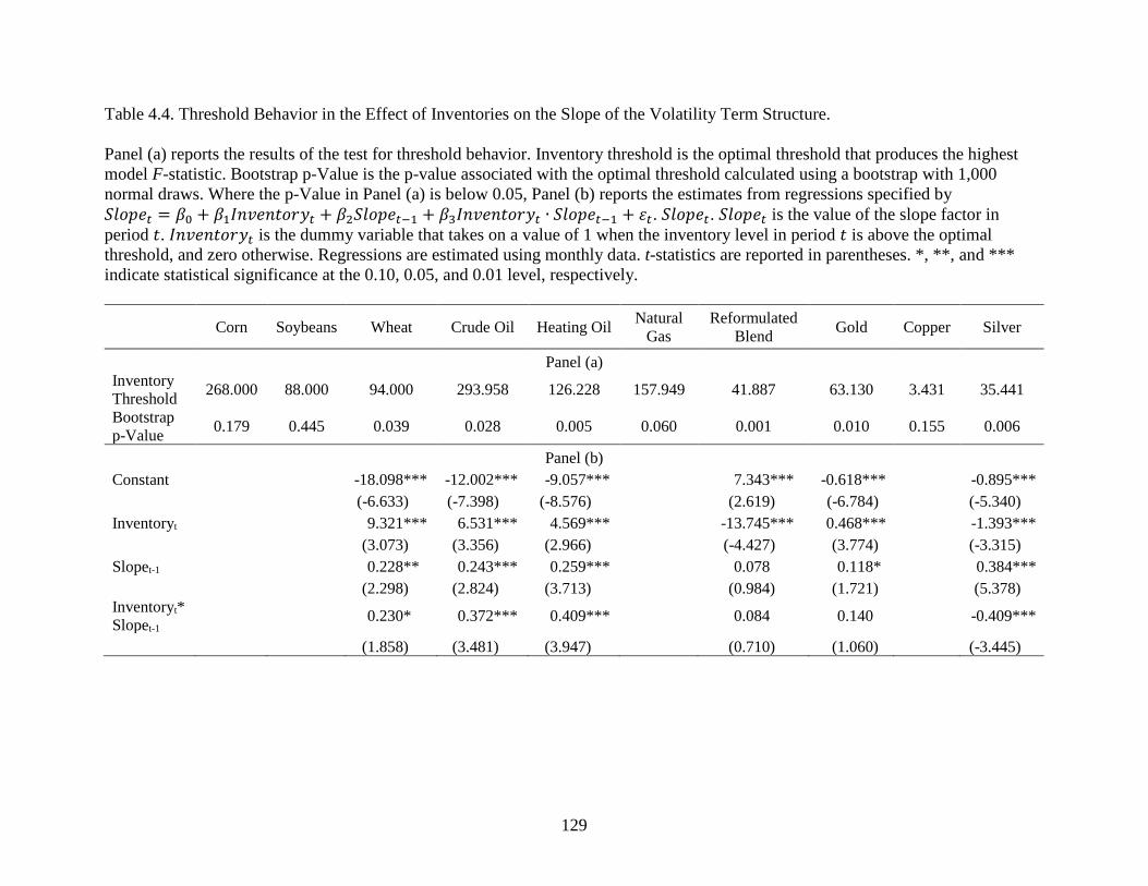
129
Table 4.4. Threshold Behavior in the Effect of Inventories on the Slope of the Volatility Term Structure. Panel (a) reports the results of the test for threshold behavior. Inventory threshold is the optimal threshold that produces the highest model F-statistic. Bootstrap p-Value is the p-value associated with the optimal threshold calculated using a bootstrap with 1,000 normal draws. Where the p-Value in Panel (a) is below 0.05, Panel (b) reports the estimates from regressions specified by 𝑆𝑆𝑙𝑙𝑙𝑙𝑙𝑙𝑣𝑣𝑡𝑡 = 𝛽𝛽0 + 𝛽𝛽1𝐼𝐼𝑛𝑛𝑣𝑣𝑣𝑣𝑛𝑛𝑡𝑡𝑙𝑙𝑟𝑟𝑦𝑦𝑡𝑡 + 𝛽𝛽2𝑆𝑆𝑙𝑙𝑙𝑙𝑙𝑙𝑣𝑣𝑡𝑡−1 + 𝛽𝛽3𝐼𝐼𝑛𝑛𝑣𝑣𝑣𝑣𝑛𝑛𝑡𝑡𝑙𝑙𝑟𝑟𝑦𝑦𝑡𝑡 ∙ 𝑆𝑆𝑙𝑙𝑙𝑙𝑙𝑙𝑣𝑣𝑡𝑡−1 + 𝜀𝜀𝑡𝑡. 𝑆𝑆𝑙𝑙𝑙𝑙𝑙𝑙𝑣𝑣𝑡𝑡. 𝑆𝑆𝑙𝑙𝑙𝑙𝑙𝑙𝑣𝑣𝑡𝑡 is the value of the slope factor in period 𝑡𝑡. 𝐼𝐼𝑛𝑛𝑣𝑣𝑣𝑣𝑛𝑛𝑡𝑡𝑙𝑙𝑟𝑟𝑦𝑦𝑡𝑡 is the dummy variable that takes on a value of 1 when the inventory level in period 𝑡𝑡 is above the optimal threshold, and zero otherwise. Regressions are estimated using monthly data. t-statistics are reported in parentheses. *, **, and *** indicate statistical significance at the 0.10, 0.05, and 0.01 level, respectively.
Corn Soybeans Wheat Crude Oil Heating Oil Natural Gas
Reformulated Blend Gold Copper Silver
Panel (a) Inventory Threshold 268.000 88.000 94.000 293.958 126.228 157.949 41.887 63.130 3.431 35.441
Bootstrap p-Value 0.179 0.445 0.039 0.028 0.005 0.060 0.001 0.010 0.155 0.006
Panel (b) Constant -18.098*** -12.002*** -9.057*** 7.343*** -0.618*** -0.895*** (-6.633) (-7.398) (-8.576) (2.619) (-6.784) (-5.340) Inventoryt 9.321*** 6.531*** 4.569*** -13.745*** 0.468*** -1.393*** (3.073) (3.356) (2.966) (-4.427) (3.774) (-3.315) Slopet-1 0.228** 0.243*** 0.259*** 0.078 0.118* 0.384*** (2.298) (2.824) (3.713) (0.984) (1.721) (5.378) Inventoryt*Slopet-1
0.230* 0.372*** 0.409*** 0.084 0.140 -0.409***
(1.858) (3.481) (3.947) (0.710) (1.060) (-3.445)

130
Table 4.5. Effect of Inventories on the Slope of the Volatility Term Structure with Daily Frequency. This table reports coefficient estimates from regressions specified by 𝑆𝑆𝑙𝑙𝑙𝑙𝑙𝑙𝑣𝑣𝑡𝑡 = 𝛽𝛽0 + 𝛽𝛽1𝐼𝐼𝑛𝑛𝑣𝑣𝑣𝑣𝑛𝑛𝑡𝑡𝑙𝑙𝑟𝑟𝑦𝑦𝑡𝑡 + 𝛽𝛽2𝑆𝑆𝑙𝑙𝑙𝑙𝑙𝑙𝑣𝑣𝑡𝑡−1 + 𝛽𝛽3𝐼𝐼𝑛𝑛𝑣𝑣𝑣𝑣𝑛𝑛𝑡𝑡𝑙𝑙𝑟𝑟𝑦𝑦𝑡𝑡 ∙ 𝑆𝑆𝑙𝑙𝑙𝑙𝑙𝑙𝑣𝑣𝑡𝑡−1 + 𝜀𝜀𝑡𝑡. 𝑆𝑆𝑙𝑙𝑙𝑙𝑙𝑙𝑣𝑣𝑡𝑡 is the value of the slope factor in period 𝑡𝑡. 𝐼𝐼𝑛𝑛𝑣𝑣𝑣𝑣𝑛𝑛𝑡𝑡𝑙𝑙𝑟𝑟𝑦𝑦𝑡𝑡 is the dummy variable that takes on a value of 1 when the inventory level in period 𝑡𝑡 is above its median, and zero otherwise. Regressions are estimated using daily data. t-statistics are reported in parentheses. *, **, and *** indicate statistical significance at the 0.10, 0.05, and 0.01 level, respectively.
Gold Copper Silver
Constant -0.487*** -4.790*** -1.292*** (-9.587) (-18.874) (-12.420) Inventory 0.273*** 1.803*** 0.254* (3.818) (4.962) (1.742) Slopet-1 0.037** 0.042*** 0.065*** (2.366) (2.978) (3.466) Inventory*Slopet-1 -0.017 0.027 -0.078*** (-0.622) (0.846) (-3.052)

131
Table 4.6. Threshold Behavior in the Effect of Inventories on the Slope of the Volatility Term Structure with Daily Frequency. Panel (a) reports the results of the test for threshold behavior. Inventory threshold is the optimal threshold that produces the highest model F-statistic. Bootstrap p-Value is the p-value associated with the optimal threshold calculated using a bootstrap with 1,000 normal draws. Where the p-Value in Panel (a) is below 0.05, Panel (b) reports the estimates from regressions specified by 𝑆𝑆𝑙𝑙𝑙𝑙𝑙𝑙𝑣𝑣𝑡𝑡 = 𝛽𝛽0 + 𝛽𝛽1𝐼𝐼𝑛𝑛𝑣𝑣𝑣𝑣𝑛𝑛𝑡𝑡𝑙𝑙𝑟𝑟𝑦𝑦𝑡𝑡 + 𝛽𝛽2𝑆𝑆𝑙𝑙𝑙𝑙𝑙𝑙𝑣𝑣𝑡𝑡−1 + 𝛽𝛽3𝐼𝐼𝑛𝑛𝑣𝑣𝑣𝑣𝑛𝑛𝑡𝑡𝑙𝑙𝑟𝑟𝑦𝑦𝑡𝑡 ∙ 𝑆𝑆𝑙𝑙𝑙𝑙𝑙𝑙𝑣𝑣𝑡𝑡−1 + 𝜀𝜀𝑡𝑡. 𝑆𝑆𝑙𝑙𝑙𝑙𝑙𝑙𝑣𝑣𝑡𝑡. 𝑆𝑆𝑙𝑙𝑙𝑙𝑙𝑙𝑣𝑣𝑡𝑡 is the value of the slope factor in period 𝑡𝑡. 𝐼𝐼𝑛𝑛𝑣𝑣𝑣𝑣𝑛𝑛𝑡𝑡𝑙𝑙𝑟𝑟𝑦𝑦𝑡𝑡 is the dummy variable that takes on a value of 1 when the inventory level in period 𝑡𝑡 is above the optimal threshold, and zero otherwise. Regressions are estimated using daily data. t-statistics are reported in parentheses. *, **, and *** indicate statistical significance at the 0.10, 0.05, and 0.01 level, respectively.
Gold Copper Silver
Panel (a) Inventory Threshold 76.123 3.844 24.893 Bootstrap p-Value 0.000 0.000 0.005
Panel (b) Constant -0.472*** -5.013*** -1.290*** (-10.702) (-18.265) (-12.388) Inventory 0.361*** 2.019*** 0.247* (4.802) (5.514) (1.695) Slopet-1 0.041*** 0.031** 0.063*** (2.962) (2.130) (3.354) Inventory*Slopet-1 -0.066* 0.064** -0.074*** (-1.954) (2.197) (-2.896)
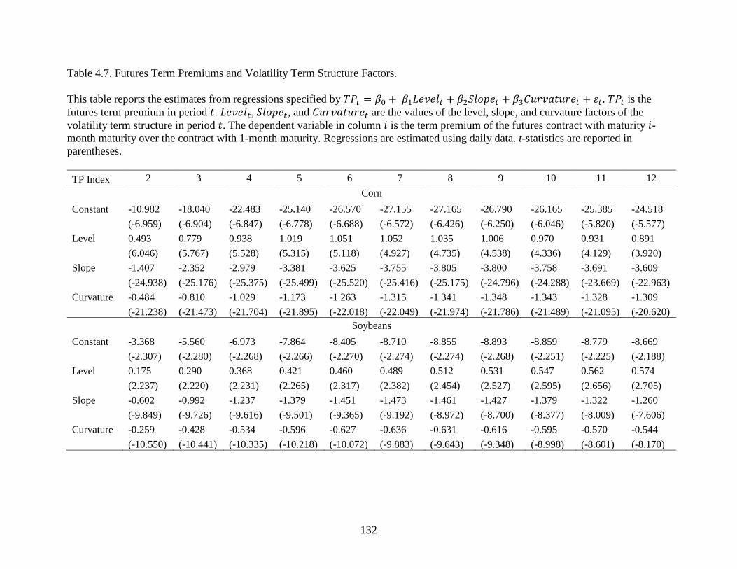
132
Table 4.7. Futures Term Premiums and Volatility Term Structure Factors. This table reports the estimates from regressions specified by 𝑇𝑇𝑅𝑅𝑡𝑡 = 𝛽𝛽0 + 𝛽𝛽1𝐿𝐿𝑣𝑣𝑣𝑣𝑣𝑣𝑙𝑙𝑡𝑡 + 𝛽𝛽2𝑆𝑆𝑙𝑙𝑙𝑙𝑙𝑙𝑣𝑣𝑡𝑡 + 𝛽𝛽3𝐶𝐶𝑢𝑢𝑟𝑟𝑣𝑣𝐶𝐶𝑡𝑡𝑢𝑢𝑟𝑟𝑣𝑣𝑡𝑡 + 𝜀𝜀𝑡𝑡. 𝑇𝑇𝑅𝑅𝑡𝑡 is the futures term premium in period 𝑡𝑡. 𝐿𝐿𝑣𝑣𝑣𝑣𝑣𝑣𝑙𝑙𝑡𝑡, 𝑆𝑆𝑙𝑙𝑙𝑙𝑙𝑙𝑣𝑣𝑡𝑡, and 𝐶𝐶𝑢𝑢𝑟𝑟𝑣𝑣𝐶𝐶𝑡𝑡𝑢𝑢𝑟𝑟𝑣𝑣𝑡𝑡 are the values of the level, slope, and curvature factors of the volatility term structure in period 𝑡𝑡. The dependent variable in column 𝑖𝑖 is the term premium of the futures contract with maturity 𝑖𝑖-month maturity over the contract with 1-month maturity. Regressions are estimated using daily data. t-statistics are reported in parentheses. TP Index 2 3 4 5 6 7 8 9 10 11 12
Corn Constant -10.982 -18.040 -22.483 -25.140 -26.570 -27.155 -27.165 -26.790 -26.165 -25.385 -24.518 (-6.959) (-6.904) (-6.847) (-6.778) (-6.688) (-6.572) (-6.426) (-6.250) (-6.046) (-5.820) (-5.577) Level 0.493 0.779 0.938 1.019 1.051 1.052 1.035 1.006 0.970 0.931 0.891 (6.046) (5.767) (5.528) (5.315) (5.118) (4.927) (4.735) (4.538) (4.336) (4.129) (3.920) Slope -1.407 -2.352 -2.979 -3.381 -3.625 -3.755 -3.805 -3.800 -3.758 -3.691 -3.609 (-24.938) (-25.176) (-25.375) (-25.499) (-25.520) (-25.416) (-25.175) (-24.796) (-24.288) (-23.669) (-22.963) Curvature -0.484 -0.810 -1.029 -1.173 -1.263 -1.315 -1.341 -1.348 -1.343 -1.328 -1.309 (-21.238) (-21.473) (-21.704) (-21.895) (-22.018) (-22.049) (-21.974) (-21.786) (-21.489) (-21.095) (-20.620)
Soybeans Constant -3.368 -5.560 -6.973 -7.864 -8.405 -8.710 -8.855 -8.893 -8.859 -8.779 -8.669 (-2.307) (-2.280) (-2.268) (-2.266) (-2.270) (-2.274) (-2.274) (-2.268) (-2.251) (-2.225) (-2.188) Level 0.175 0.290 0.368 0.421 0.460 0.489 0.512 0.531 0.547 0.562 0.574 (2.237) (2.220) (2.231) (2.265) (2.317) (2.382) (2.454) (2.527) (2.595) (2.656) (2.705) Slope -0.602 -0.992 -1.237 -1.379 -1.451 -1.473 -1.461 -1.427 -1.379 -1.322 -1.260 (-9.849) (-9.726) (-9.616) (-9.501) (-9.365) (-9.192) (-8.972) (-8.700) (-8.377) (-8.009) (-7.606) Curvature -0.259 -0.428 -0.534 -0.596 -0.627 -0.636 -0.631 -0.616 -0.595 -0.570 -0.544 (-10.550) (-10.441) (-10.335) (-10.218) (-10.072) (-9.883) (-9.643) (-9.348) (-8.998) (-8.601) (-8.170)

133
Table 4.7 (cont.) TP Index 2 3 4 5 6 7 8 9 10 11 12
Wheat Constant 2.405 5.179 7.882 10.344 12.519 14.415 16.063 17.495 18.746 19.843 20.812 (1.271) (1.649) (1.991) (2.303) (2.589) (2.850) (3.085) (3.294) (3.477) (3.635) (3.767) Level -0.207 -0.385 -0.529 -0.641 -0.726 -0.790 -0.837 -0.872 -0.897 -0.915 -0.927 (-2.400) (-2.683) (-2.921) (-3.120) (-3.284) (-3.416) (-3.518) (-3.591) (-3.640) (-3.666) (-3.673) Slope 0.146 0.328 0.506 0.665 0.801 0.916 1.013 1.094 1.163 1.222 1.272 (2.423) (3.284) (4.020) (4.659) (5.216) (5.703) (6.125) (6.487) (6.792) (7.045) (7.251) Curvature 0.077 0.151 0.210 0.253 0.281 0.298 0.305 0.307 0.304 0.298 0.291 (2.868) (3.369) (3.716) (3.942) (4.070) (4.120) (4.108) (4.046) (3.948) (3.824) (3.684)
Crude Oil Constant -0.665 -1.178 -1.588 -1.923 -2.201 -2.434 -2.631 -2.797 -2.939 -3.061 -3.167 (-0.613) (-0.634) (-0.656) (-0.676) (-0.693) (-0.707) (-0.718) (-0.725) (-0.730) (-0.732) (-0.733) Level 0.023 0.049 0.075 0.098 0.120 0.139 0.156 0.171 0.184 0.196 0.206 (0.509) (0.636) (0.744) (0.835) (0.911) (0.974) (1.026) (1.068) (1.102) (1.129) (1.150) Slope -0.028 -0.040 -0.044 -0.043 -0.041 -0.037 -0.033 -0.029 -0.024 -0.020 -0.016 (-0.769) (-0.639) (-0.535) (-0.450) (-0.378) (-0.317) (-0.264) (-0.218) (-0.177) (-0.140) (-0.108) Curvature -0.022 -0.031 -0.036 -0.039 -0.041 -0.042 -0.044 -0.045 -0.046 -0.047 -0.048 (-0.923) (-0.779) (-0.688) (-0.630) (-0.593) (-0.569) (-0.553) (-0.541) (-0.532) (-0.524) (-0.518)

134
Table 4.7 (cont.) TP Index 2 3 4 5 6 7 8 9 10 11 12
Heating Oil Constant -1.858 -2.758 -3.051 -2.952 -2.602 -2.093 -1.490 -0.835 -0.158 0.520 1.186 (-1.124) (-1.011) (-0.899) (-0.782) (-0.654) (-0.514) (-0.362) (-0.201) (-0.038) (0.123) (0.275) Level -0.029 -0.052 -0.067 -0.071 -0.066 -0.056 -0.040 -0.022 -0.001 0.019 0.040 (-0.411) (-0.456) (-0.467) (-0.446) (-0.398) (-0.325) (-0.232) (-0.124) (-0.008) (0.109) (0.222) Slope -0.171 -0.263 -0.295 -0.283 -0.241 -0.178 -0.102 -0.018 0.069 0.157 0.243 (-3.002) (-2.793) (-2.520) (-2.176) (-1.757) (-1.266) (-0.716) (-0.126) (0.478) (1.071) (1.629) Curvature -0.090 -0.148 -0.183 -0.203 -0.210 -0.209 -0.202 -0.191 -0.177 -0.162 -0.146 (-3.141) (-3.126) (-3.115) (-3.093) (-3.045) (-2.960) (-2.832) (-2.659) (-2.446) (-2.204) (-1.945)
Natural Gas Constant -12.748 -17.681 -19.326 -19.409 -18.641 -17.338 -15.657 -13.696 -11.527 -9.206 -6.782 (-2.937) (-2.544) (-2.264) (-2.052) (-1.872) (-1.701) (-1.522) (-1.326) (-1.112) (-0.883) (-0.644) Level 0.220 0.203 0.086 -0.063 -0.208 -0.338 -0.448 -0.540 -0.616 -0.678 -0.729 (1.234) (0.713) (0.245) (-0.161) (-0.510) (-0.808) (-1.062) (-1.275) (-1.449) (-1.586) (-1.689) Slope -0.149 -0.229 -0.286 -0.331 -0.363 -0.383 -0.391 -0.389 -0.377 -0.358 -0.333 (-1.935) (-1.856) (-1.888) (-1.968) (-2.052) (-2.116) (-2.141) (-2.119) (-2.049) (-1.934) (-1.780) Curvature -0.217 -0.342 -0.424 -0.476 -0.505 -0.516 -0.513 -0.499 -0.476 -0.446 -0.411 (-3.829) (-3.768) (-3.796) (-3.847) (-3.881) (-3.876) (-3.816) (-3.695) (-3.511) (-3.271) (-2.985)

135
Table 4.7 (cont.) TP Index 2 3 4 5 6 7 8 9 10 11 12
Reformulated Blend Constant -11.554 -17.954 -21.645 -23.780 -24.949 -25.475 -25.553 -25.312 -24.841 -24.209 -23.466 (-4.137) (-4.035) (-4.026) (-4.075) (-4.149) (-4.218) (-4.254) (-4.235) (-4.149) (-3.997) (-3.793) Level 0.390 0.624 0.764 0.847 0.896 0.922 0.935 0.939 0.937 0.933 0.926 (3.862) (3.871) (3.924) (4.010) (4.114) (4.218) (4.299) (4.339) (4.324) (4.254) (4.135) Slope -0.375 -0.587 -0.711 -0.780 -0.812 -0.817 -0.802 -0.771 -0.729 -0.679 -0.624 (-4.909) (-4.826) (-4.839) (-4.894) (-4.946) (-4.955) (-4.888) (-4.724) (-4.459) (-4.107) (-3.693) Curvature -0.017 -0.009 0.004 0.016 0.026 0.037 0.049 0.062 0.076 0.092 0.109 (-0.468) (-0.152) (0.053) (0.203) (0.332) (0.465) (0.614) (0.783) (0.966) (1.156) (1.342)
Gold Constant 0.917 1.578 2.049 2.379 2.606 2.760 2.861 2.924 2.961 2.979 2.986 (3.210) (3.336) (3.469) (3.607) (3.747) (3.889) (4.027) (4.160) (4.284) (4.397) (4.497) Level -0.071 -0.123 -0.160 -0.185 -0.203 -0.215 -0.223 -0.228 -0.231 -0.233 -0.234 (-4.097) (-4.260) (-4.431) (-4.609) (-4.792) (-4.975) (-5.155) (-5.328) (-5.490) (-5.637) (-5.768) Slope 0.595 1.018 1.312 1.512 1.643 1.727 1.776 1.802 1.812 1.810 1.802 (7.895) (8.147) (8.409) (8.677) (8.946) (9.212) (9.468) (9.707) (9.924) (10.115) (10.275) Curvature 0.606 1.008 1.262 1.412 1.489 1.516 1.510 1.483 1.442 1.394 1.343 (31.514) (31.651) (31.756) (31.815) (31.817) (31.746) (31.594) (31.351) (31.013) (30.580) (30.058)

136
Table 4.7 (cont.) TP Index 2 3 4 5 6 7 8 9 10 11 12
Copper Constant -1.355 -2.370 -3.136 -3.720 -4.166 -4.507 -4.768 -4.968 -5.121 -5.239 -5.328 (-1.911) (-1.977) (-2.036) (-2.086) (-2.124) (-2.149) (-2.162) (-2.162) (-2.152) (-2.134) (-2.109) Level 0.042 0.077 0.109 0.136 0.161 0.183 0.203 0.221 0.237 0.252 0.265 (1.434) (1.570) (1.712) (1.855) (1.992) (2.120) (2.236) (2.336) (2.422) (2.492) (2.550) Slope -0.208 -0.344 -0.429 -0.477 -0.499 -0.502 -0.492 -0.473 -0.449 -0.421 -0.392 (-5.174) (-5.071) (-4.921) (-4.728) (-4.495) (-4.230) (-3.941) (-3.640) (-3.334) (-3.032) (-2.741) Curvature -0.197 -0.333 -0.428 -0.495 -0.541 -0.573 -0.594 -0.608 -0.616 -0.621 -0.622 (-9.941) (-9.951) (-9.956) (-9.938) (-9.884) (-9.790) (-9.655) (-9.482) (-9.281) (-9.058) (-8.824)
Silver Constant 2.749 4.681 5.985 6.822 7.322 7.587 7.689 7.684 7.609 7.490 7.348 (5.874) (5.966) (6.048) (6.119) (6.175) (6.214) (6.235) (6.235) (6.214) (6.174) (6.116) Level -0.065 -0.109 -0.136 -0.150 -0.156 -0.157 -0.153 -0.147 -0.140 -0.133 -0.125 (-4.057) (-4.024) (-3.974) (-3.907) (-3.823) (-3.721) (-3.602) (-3.469) (-3.324) (-3.169) (-3.007) Slope 1.388 2.411 3.148 3.666 4.023 4.264 4.420 4.518 4.575 4.603 4.612 (22.518) (23.331) (24.150) (24.964) (25.758) (26.512) (27.209) (27.831) (28.365) (28.804) (29.145) Curvature 0.965 1.645 2.104 2.399 2.576 2.671 2.708 2.708 2.683 2.643 2.594 (63.610) (64.638) (65.555) (66.347) (66.988) (67.449) (67.708) (67.748) (67.566) (67.169) (66.576)

137
Table 4.8. Incremental Futures Term Premiums and Volatility Term Structure Factors. This table reports the estimates from regressions specified by 𝐼𝐼𝑇𝑇𝑅𝑅𝑡𝑡 = 𝛽𝛽0 + 𝛽𝛽1𝐿𝐿𝑣𝑣𝑣𝑣𝑣𝑣𝑙𝑙𝑡𝑡 + 𝛽𝛽2𝑆𝑆𝑙𝑙𝑙𝑙𝑙𝑙𝑣𝑣𝑡𝑡 + 𝛽𝛽3𝐶𝐶𝑢𝑢𝑟𝑟𝑣𝑣𝐶𝐶𝑡𝑡𝑢𝑢𝑟𝑟𝑣𝑣𝑡𝑡 + 𝜀𝜀𝑡𝑡. 𝐼𝐼𝑇𝑇𝑅𝑅𝑡𝑡 is the incremental futures term premium in period 𝑡𝑡. 𝐿𝐿𝑣𝑣𝑣𝑣𝑣𝑣𝑙𝑙𝑡𝑡, 𝑆𝑆𝑙𝑙𝑙𝑙𝑙𝑙𝑣𝑣𝑡𝑡, and 𝐶𝐶𝑢𝑢𝑟𝑟𝑣𝑣𝐶𝐶𝑡𝑡𝑢𝑢𝑟𝑟𝑣𝑣𝑡𝑡 are the values of the level, slope, and curvature factors of the volatility term structure in period 𝑡𝑡. The dependent variable in column 𝑖𝑖 is the incremental term premium of the futures contract 𝑖𝑖-month maturity over the contract with (𝑖𝑖 − 1)-month maturity. Regressions are estimated using daily data. t-statistics are reported in parentheses. ITP Index 2 3 4 5 6 7 8 9 10 11 12
Corn Constant -10.982 -7.058 -4.442 -2.658 -1.430 -0.585 -0.010 0.375 0.625 0.780 0.867 (-6.959) (-6.758) (-6.335) (-5.382) (-3.703) (-1.707) (-0.030) (1.151) (1.947) (2.493) (2.879) Level 0.493 0.286 0.159 0.081 0.032 0.001 -0.018 -0.029 -0.036 -0.039 -0.040 (6.046) (5.293) (4.395) (3.168) (1.596) (0.071) (-1.034) (-1.724) (-2.144) (-2.410) (-2.587) Slope -1.407 -0.945 -0.627 -0.403 -0.243 -0.130 -0.050 0.005 0.042 0.067 0.082 (-24.938) (-25.306) (-25.006) (-22.807) (-17.615) (-10.600) (-4.260) (0.420) (3.680) (5.962) (7.601) Curvature -0.484 -0.326 -0.219 -0.144 -0.090 -0.052 -0.026 -0.007 0.006 0.014 0.020 (-21.238) (-21.633) (-21.614) (-20.145) (-16.204) (-10.604) (-5.408) (-1.516) (1.217) (3.139) (4.520)
Soybeans Constant -3.368 -2.192 -1.413 -0.891 -0.541 -0.305 -0.145 -0.038 0.034 0.080 0.110 (-2.307) (-2.224) (-2.144) (-1.975) (-1.577) (-0.996) (-0.479) (-0.123) (0.108) (0.262) (0.368) Level 0.175 0.115 0.077 0.054 0.039 0.029 0.023 0.019 0.016 0.014 0.013 (2.237) (2.180) (2.192) (2.217) (2.102) (1.778) (1.419) (1.152) (0.979) (0.870) (0.802) Slope -0.602 -0.391 -0.245 -0.143 -0.071 -0.022 0.012 0.034 0.048 0.057 0.062 (-9.849) (-9.478) (-8.874) (-7.551) (-4.975) (-1.725) (0.913) (2.638) (3.731) (4.449) (4.945) Curvature -0.259 -0.169 -0.106 -0.062 -0.031 -0.009 0.005 0.015 0.021 0.025 0.027 (-10.550) (-10.207) (-9.586) (-8.161) (-5.358) (-1.825) (1.030) (2.883) (4.042) (4.791) (5.297)

138
Table 4.8 (cont.) ITP Index 2 3 4 5 6 7 8 9 10 11 12
Wheat Constant 2.405 2.774 2.703 2.462 2.175 1.897 1.647 1.433 1.251 1.097 0.969 (1.271) (2.203) (3.164) (4.031) (4.513) (4.463) (4.096) (3.667) (3.292) (2.992) (2.760) Level -0.207 -0.178 -0.144 -0.112 -0.085 -0.064 -0.047 -0.035 -0.025 -0.018 -0.013 (-2.400) (-3.087) (-3.676) (-4.012) (-3.874) (-3.293) (-2.573) (-1.937) (-1.442) (-1.069) (-0.790) Slope 0.146 0.182 0.178 0.159 0.137 0.115 0.097 0.081 0.069 0.059 0.051 (2.423) (4.550) (6.561) (8.202) (8.920) (8.533) (7.563) (6.546) (5.696) (5.037) (4.540) Curvature 0.077 0.074 0.059 0.043 0.028 0.017 0.008 0.001 -0.003 -0.006 -0.008 (2.868) (4.093) (4.838) (4.900) (4.103) (2.733) (1.354) (0.258) (-0.540) (-1.106) (-1.507)
Crude Oil Constant -0.665 -0.513 -0.410 -0.335 -0.278 -0.233 -0.196 -0.167 -0.142 -0.122 -0.105 (-0.613) (-0.657) (-0.699) (-0.719) (-0.707) (-0.670) (-0.620) (-0.569) (-0.523) (-0.483) (-0.449) Level 0.023 0.026 0.026 0.024 0.021 0.019 0.017 0.015 0.013 0.012 0.010 (0.509) (0.807) (1.056) (1.231) (1.317) (1.325) (1.286) (1.228) (1.168) (1.113) (1.065) Slope -0.028 -0.012 -0.004 0.001 0.003 0.004 0.004 0.004 0.004 0.004 0.004 (-0.769) (-0.451) (-0.186) (0.032) (0.199) (0.316) (0.392) (0.440) (0.471) (0.492) (0.508) Curvature -0.022 -0.010 -0.005 -0.003 -0.002 -0.002 -0.001 -0.001 -0.001 -0.001 -0.001 (-0.923) (-0.571) (-0.373) (-0.272) (-0.229) (-0.215) (-0.211) (-0.209) (-0.205) (-0.198) (-0.190)
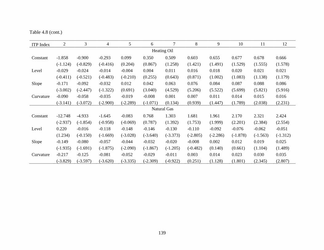
139
Table 4.8 (cont.) ITP Index 2 3 4 5 6 7 8 9 10 11 12
Heating Oil Constant -1.858 -0.900 -0.293 0.099 0.350 0.509 0.603 0.655 0.677 0.678 0.666 (-1.124) (-0.829) (-0.416) (0.204) (0.867) (1.258) (1.421) (1.491) (1.529) (1.555) (1.578) Level -0.029 -0.024 -0.014 -0.004 0.004 0.011 0.016 0.018 0.020 0.021 0.021 (-0.411) (-0.521) (-0.483) (-0.210) (0.255) (0.643) (0.871) (1.002) (1.083) (1.138) (1.179) Slope -0.171 -0.092 -0.032 0.012 0.042 0.063 0.076 0.084 0.087 0.088 0.086 (-3.002) (-2.447) (-1.322) (0.691) (3.040) (4.529) (5.206) (5.522) (5.699) (5.821) (5.916) Curvature -0.090 -0.058 -0.035 -0.019 -0.008 0.001 0.007 0.011 0.014 0.015 0.016 (-3.141) (-3.072) (-2.900) (-2.289) (-1.071) (0.134) (0.939) (1.447) (1.789) (2.038) (2.231)
Natural Gas Constant -12.748 -4.933 -1.645 -0.083 0.768 1.303 1.681 1.961 2.170 2.321 2.424 (-2.937) (-1.854) (-0.958) (-0.069) (0.787) (1.392) (1.753) (1.999) (2.201) (2.384) (2.554) Level 0.220 -0.016 -0.118 -0.148 -0.146 -0.130 -0.110 -0.092 -0.076 -0.062 -0.051 (1.234) (-0.150) (-1.669) (-3.028) (-3.640) (-3.373) (-2.805) (-2.286) (-1.878) (-1.563) (-1.312) Slope -0.149 -0.080 -0.057 -0.044 -0.032 -0.020 -0.008 0.002 0.012 0.019 0.025 (-1.935) (-1.691) (-1.875) (-2.090) (-1.867) (-1.205) (-0.482) (0.140) (0.661) (1.104) (1.489) Curvature -0.217 -0.125 -0.081 -0.052 -0.029 -0.011 0.003 0.014 0.023 0.030 0.035 (-3.829) (-3.597) (-3.620) (-3.335) (-2.309) (-0.922) (0.251) (1.128) (1.801) (2.345) (2.807)

140
Table 4.8 (cont.) ITP Index 2 3 4 5 6 7 8 9 10 11 12
Reformulated Blend Constant -11.554 -6.400 -3.691 -2.135 -1.168 -0.526 -0.078 0.241 0.471 0.633 0.743 (-4.137) (-3.820) (-3.690) (-3.186) (-1.915) (-0.794) (-0.109) (0.320) (0.616) (0.836) (1.008) Level 0.390 0.233 0.140 0.084 0.048 0.027 0.013 0.004 -0.001 -0.005 -0.007 (3.862) (3.842) (3.869) (3.442) (2.193) (1.105) (0.487) (0.147) (-0.051) (-0.172) (-0.249) Slope -0.375 -0.212 -0.124 -0.070 -0.032 -0.005 0.015 0.031 0.042 0.050 0.055 (-4.909) (-4.633) (-4.542) (-3.801) (-1.930) (-0.273) (0.785) (1.489) (2.007) (2.415) (2.752) Curvature -0.017 0.008 0.013 0.012 0.011 0.011 0.012 0.013 0.015 0.016 0.017 (-0.468) (0.375) (0.964) (1.338) (1.335) (1.226) (1.223) (1.311) (1.447) (1.605) (1.768)
Gold Constant 0.917 0.662 0.471 0.330 0.227 0.153 0.101 0.063 0.037 0.019 0.006 (3.210) (3.519) (3.942) (4.470) (4.805) (4.167) (2.793) (1.668) (0.940) (0.472) (0.159) Level -0.071 -0.052 -0.037 -0.026 -0.018 -0.012 -0.008 -0.005 -0.003 -0.002 -0.001 (-4.097) (-4.495) (-5.043) (-5.730) (-6.178) (-5.380) (-3.628) (-2.186) (-1.252) (-0.651) (-0.249) Slope 0.595 0.423 0.294 0.200 0.132 0.083 0.049 0.026 0.010 -0.001 -0.008 (7.895) (8.510) (9.319) (10.244) (10.542) (8.572) (5.186) (2.569) (0.920) (-0.124) (-0.817) Curvature 0.606 0.402 0.255 0.150 0.077 0.027 -0.006 -0.027 -0.040 -0.048 -0.051 (31.514) (31.782) (31.690) (30.173) (24.142) (10.932) (-2.488) (-10.729) (-15.294) (-17.960) (-19.632)

141
Table 4.8 (cont.) ITP Index 2 3 4 5 6 7 8 9 10 11 12
Copper Constant -1.355 -1.014 -0.767 -0.583 -0.446 -0.341 -0.261 -0.200 -0.153 -0.117 -0.090 (-1.911) (-2.054) (-2.153) (-2.133) (-1.954) (-1.665) (-1.359) (-1.089) (-0.871) (-0.698) (-0.563) Level 0.042 0.036 0.031 0.028 0.025 0.022 0.020 0.018 0.016 0.015 0.013 (1.434) (1.752) (2.121) (2.450) (2.628) (2.630) (2.523) (2.380) (2.241) (2.120) (2.018) Slope -0.208 -0.136 -0.085 -0.048 -0.022 -0.003 0.010 0.019 0.024 0.028 0.029 (-5.174) (-4.878) (-4.218) (-3.109) (-1.682) (-0.262) (0.912) (1.794) (2.438) (2.909) (3.260) Curvature -0.197 -0.136 -0.095 -0.067 -0.046 -0.032 -0.021 -0.014 -0.008 -0.004 -0.001 (-9.941) (-9.877) (-9.568) (-8.726) (-7.289) (-5.580) (-3.988) (-2.690) (-1.687) (-0.922) (-0.336)
Silver Constant 2.749 1.932 1.304 0.837 0.501 0.264 0.103 -0.005 -0.075 -0.118 -0.143 (5.874) (6.082) (6.244) (6.180) (5.419) (3.593) (1.482) (-0.078) (-1.075) (-1.712) (-2.134) Level -0.065 -0.043 -0.027 -0.015 -0.006 -0.000 0.003 0.006 0.007 0.008 0.008 (-4.057) (-3.962) (-3.712) (-3.127) (-1.914) (-0.130) (1.437) (2.402) (2.944) (3.259) (3.454) Slope 1.388 1.023 0.736 0.518 0.357 0.240 0.157 0.098 0.057 0.028 0.009 (22.518) (24.449) (26.772) (29.065) (29.359) (24.781) (17.186) (10.665) (6.146) (3.115) (1.039) Curvature 0.965 0.679 0.459 0.295 0.177 0.094 0.038 -0.000 -0.025 -0.040 -0.049 (63.610) (65.932) (67.770) (67.221) (59.169) (39.549) (16.753) (-0.150) (-10.972) (-17.889) (-22.477)

142
Figure 4.1. Average Futures Volatility Term Structure. This figure plots average futures volatility during the sample period as a function of time to expiration. Volatilities of all contracts are expressed as a percentage of the volatility of the 1-month contract. Time to expiration is measured in months.
40%
60%
80%
100%
0 5 10
Vola
tility
(Rel
ativ
e to
1st
)
Time to Expiration
Corn
40%
60%
80%
100%
0 5 10
Vola
tility
(Rel
ativ
e to
1st
)
Time to Expiration
Soybeans
40%
60%
80%
100%
0 5 10
Vola
tility
(Rel
ativ
e to
1st
)
Time to Expiration
Wheat
40%
60%
80%
100%
0 5 10
Vola
tility
(Rel
ativ
e to
1st
)
Time to Expiration
Crude Oil

143
Figure 4.1 (cont.)
40%
60%
80%
100%
0 5 10
Vola
tility
(Rel
ativ
e to
1st
)
Time to Expiration
Heating Oil
40%
60%
80%
100%
0 5 10
Vola
tility
(Rel
ativ
e to
1st
)
Time to Expiration
Natural Gas
40%
60%
80%
100%
0 5 10
Vola
tility
(Rel
ativ
e to
1st
)
Time to Expiration
Reformulated Blend
40%
60%
80%
100%
0 5 10
Vola
tility
(Rel
ativ
e to
1st
)
Time to Expiration
Gold
40%
60%
80%
100%
0 5 10
Vola
tility
(Rel
ativ
e to
1st
)
Time to Expiration
Copper
40%
60%
80%
100%
0 5 10
Vola
tility
(Rel
ativ
e to
1st
)
Time to Expiration
Silver

144
Figure 4.2. Time-Series Behavior of the Futures Volatility Slope Factor and Inventories. This figure plots the 60-month moving average of the volatility slope factor and 95% confidence bands on the left axis. To obtain the moving average we regress the slope factor on its first lag, its twelfth lag, and a constant within each window to account for the autoregressive behavior of the slope factor and potential seasonality (𝑆𝑆𝑙𝑙𝑙𝑙𝑙𝑙𝑣𝑣𝑡𝑡 = 𝛽𝛽0 + 𝛽𝛽1𝑆𝑆𝑙𝑙𝑙𝑙𝑙𝑙𝑣𝑣𝑡𝑡−1 + 𝛽𝛽2𝑆𝑆𝑙𝑙𝑙𝑙𝑙𝑙𝑣𝑣𝑡𝑡−12 + 𝜀𝜀𝑡𝑡). We then calculate the mean of the series as 𝔼𝔼(𝑆𝑆𝑙𝑙𝑙𝑙𝑙𝑙𝑣𝑣𝑡𝑡) = 𝛽𝛽0/(1 − 𝛽𝛽1 − 𝛽𝛽2). 60-month moving average of inventory levels is plotted on the right axis.
Corn
Soybeans
Wheat
Crude Oil
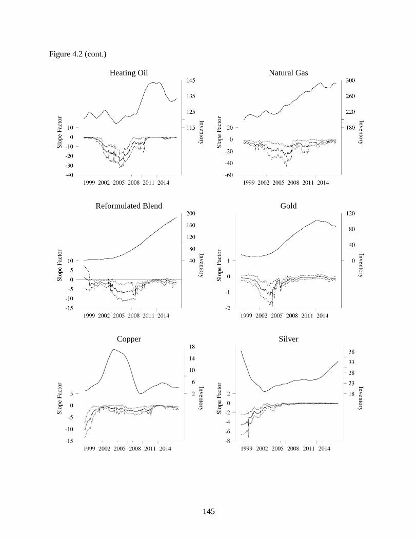
145
Figure 4.2 (cont.)
Heating Oil
Natural Gas
Reformulated Blend
Gold
Copper
Silver

146
Figure 4.3. Average Futures Term Premiums. This figure plots the futures term premiums as a function of time to expiration. Future term premium with time to expiration 𝑖𝑖 is the term premium of the contract with 𝑖𝑖-month maturity over the contract with 1-month maturity.
-30%
-10%
10%
30%
50%
0 5 10Term
Pre
miu
m
Time to Expiration
Corn
-30%
-10%
10%
30%
50%
0 5 10Term
Pre
miu
m
Time to Expiration
Soybeans
-30%
-10%
10%
30%
50%
0 5 10Term
Pre
miu
m
Time to Expiration
Wheat
-30%
-10%
10%
30%
50%
0 5 10Term
Pre
miu
m
Time to Expiration
Crude Oil

147
Figure 4.3 (cont.)
-30%
-10%
10%
30%
50%
0 5 10Term
Pre
miu
m
Time to Expiration
Heating Oil
-30%
-10%
10%
30%
50%
0 5 10Term
Pre
miu
m
Time to Expiration
Natural Gas
-30%
-10%
10%
30%
50%
0 5 10Term
Pre
miu
m
Time to Expiration
Reformulated Blend
-30%
-10%
10%
30%
50%
0 5 10Term
Pre
miu
m
Time to Expiration
Gold
-30%
-10%
10%
30%
50%
0 5 10Term
Pre
miu
m
Time to Expiration
Copper
-30%
-10%
10%
30%
50%
0 5 10Term
Pre
miu
m
Time to Expiration
Silver

148
CHAPTER 5: OVERALL CONCLUSION
The three essays of this dissertation empirically examine the time-series behavior of
volatility and information content of futures markets. The first and third essays examine futures
volatility from two different perspectives – structural change and term structure – while the
second essay deals with forecasting in interest rate futures.
In the first essay, we find that trigonometric functions work well in capturing shifts in
futures volatility, reducing model persistence. Reduced model persistence affects the quality of
forecasts, an issue related to the topic of the second essay. The findings of the second essay
indicate a convergence of the predictive information in interest rate futures across the regions
examined in the study, a phenomenon partially explained by monetary policies and
macroeconomic conditions.
Another finding documented in the first essay is that volatility shifts do not appear to be
coincident in futures with different maturities, suggesting that futures volatility term structure
changes over time. Taking a deeper look at the term structure of futures volatility in the third
essay, we find that all but one market in our study had a statistically flat volatility term structure
sometime during the sample period. Further evidence shows that the slope of the volatility term
structure is related to inventory levels and futures term premiums.

149
REFERENCES
Anderson, R. W., & Danthine, J. P. (1983). The Time Pattern of Hedging and the Volatility of Futures Prices. The Review of Economic Studies, 50(2), 249.
Bessembinder, H., Coughenour, J. F., Seguin, P. J., & Smoller, M. M. (1996). Is There a Term
Structure of Futures Volatilities? Reevaluating the Samuelson Hypothesis. The Journal of Derivatives, 4(2), 45–58.
Brooks, R. (2012). Samuelson Hypothesis and Carry Arbitrage. Journal of Derivatives, 20(2),
37–65. Brooks, R., Cline, B. N., & Enders, W. (2015). A comparison of the information in the LIBOR
and CMT term structures of interest rates. Journal of Banking & Finance, 54, 239–253. Diebold, F. X., & Li, C. (2006). Forecasting the term structure of government bond yields.
Journal of Econometrics, 130, 337–364. Diebold, F. X., Li, C., & Yue, V. Z. (2008). Global yield curve dynamics and interactions: A
dynamic Nelson–Siegel approach. Journal of Econometrics, 146(2), 351–363. Enders, W., & Holt, M. T. (2012). Sharp Breaks or Smooth Shifts? an Investigation of the
Evolution of Primary Commodity Prices. American Journal of Agricultural Economics, 94(3), 659–673.
Fama, E. F. (1984). The information in the term structure. Journal of Financial Economics,
13(4), 509–528. Gallant, A. R. (1981). On the bias in flexible functional forms and an essentially unbiased form.
Journal of Econometrics, 15(2), 211–245. Hafner, C. M., & Herwartz, H. (2006). Volatility impulse responses for multivariate GARCH
models: An exchange rate illustration. Journal of International Money and Finance, 25(5), 719–740.
Hillebrand, E. (2005). Neglecting parameter changes in GARCH models. Journal of
Econometrics, 129(1–2), 121–138. Miranda-Agrippino, S., & Rey, H. (2015). World Asset Markets and the Global Financial Cycle.
NBER Working Paper Series, 21722.

150
Myers, R. J., Johnson, S. R., Helmar, M., & Baumes, H. (2014). Long-run and Short-run Co-movements in Energy Prices and the Prices of Agricultural Feedstocks for Biofuel. American Journal of Agricultural Economics, 96(4), 991–1008.
Nelson, C. R., & Siegel, A. F. (1987). Parsimonious Modeling of Yield Curves. Journal of
Business, 60, 473–489. Perron, P. (1989). The Great Crash, the Oil Price Shock, and the Unit Root Hypothesis.
Econometrica, 57(6), 1361. Rey, H. (2015). Dilemma not Trilemma: The Global Financial Cycle and Monetary Policy
Independence. NBER Working Paper Series, 21162. Samuelson, P. A. (1965). Proof That Properly Anticipated Prices Fluctuate Randomly. Industrial
Management Review, 6(2), 41–49. Wright, J. H. (2011). Term Premia and Inflation Uncertainty: Empirical Evidence from an
International Panel Dataset. The American Economic Review, 101(4), 1514–1534.