essays on price discovery and volatility dynamics in the

Essays on Price Discovery and Volatility

Dynamics in the Foreign Exchange Market

by Fei Su

Principle Supervisor: A/Prof Jianxin, Wang

Supervisory Committee: Prof Xuezhong (Tony), He

Prof Talis Putnins

Prof Douglas Foster

A thesis submitted in fulfilment of the requirements

For the degree of Doctor of Philosophy

In the

Finance Discipline Group

UTS Business School

University of Technology Sydney

June 2018

i

Declaration of Authorship

I, Fei Su, clarify that the work in this thesis has not previously been submitted for

a degree nor has it been submitted as part of requirements for a degree except as

fully acknowledged within the text. I also clarify that the thesis has been written

by me. Any help that I have received in my research work and the preparation of

the thesis itself has been acknowledged. In addition, I certify that all information

sources and literature used are indicated in the thesis.

Moreover, I declare that one paper titled “Global Price Discovery in the Australian

Dollar Market and Its Determinants”, which is drawn from Chapter 2, has been

accepted for publication and is forthcoming in the Pacific-Basin Finance Journal.

This chapter is a collaboration work with Jingjing Zhang from Nanjing Audit

University, China. I contribute by developing research ideas, conducting empirical

analyses, and writing up. My co-author contributes by providing constructive

comments and improving the writing.

Signature____________

Date____________

ii

Acknowledgements

When I completed my bachelor’s degree in 2007, I never thought I would

undertake further studies abroad. Ten years later, I am deeply grateful for the

valuable support I received during my Ph.D. study at the University of Technology,

Sydney.

At this moment, I would like to send my greatest gratitude to A/Prof Jianxin Wang,

my principle supervisor, for providing the invaluable resources and support. I am

also indebted to the other three members of the supervisory committee, Prof

Xuezhong He, Prof Talis Putnins, and Prof Douglas Foster who provided me with

innumerable valuable comments and suggestions. I would also like to thank A/Prof

Christina Nikitopoulos Sklibosios, completing this thesis won’t be possible without

her endless support and encouragement. In addition, conversations with Dr.

Jingjing Zhang from Nanjing Audit University, Dr. Heng-guo Zhang from Fudan

University, and Dr. Xu Feng from Tianjin University have been very helpful. I am

grateful to the external examiners of the thesis, Prof Hiroshi Moriyasu from

Nagasaki University and one anonymous examiner. This thesis benefits

substantially from their constructive and detailed comments. Moreover, I received

valuable comments from conference participants at the 2016 International

Conference on Applied Financial Economics in Shanghai and 2016 Auckland

Finance Meeting. I also thank Prof Jun-Koo Kang (editor of the Pacific-Basin

Finance Journal), and one anonymous referee for constructive comments.

I am thankful for my colleagues at the Finance Discipline Group, Huong Nguyen,

Marta Khomyn, Ran Xiao, Jing Sun, Dr. Yajun Xiao, and Dr. Chi-Chung Sui, who have

been a source of both inspiration and fun during my four years at UTS. I also would

like to gratefully acknowledge the generous financial support from the UTS

Business School and the University of Technology, Sydney.

Last but not least, special thanks go to my parents, my wife, and my two beloved

children. This dissertation is dedicated to them.

iii

Table of Contents

Declaration of Authorship …………..………….………….………….………….……………..….……..i

Acknowledgements ……………………….………….………….……………….….…………………….…ii

List of Figures ………………..………….………….………….………….…………….……………..…….…vi

List of Tables …………….………….………….………….………….………….…………….………………vii

Abstract ..…………………………………………………………………………………………….……….……ix

Chapter 1 Introduction ………….………….………….………….………………………..……………...1

Chapter 2 Global Price Discovery in the Foreign Exchange Market and Its

Determinants: Evidence from the Australian Dollar ………….........………………..…….6

2.1 Introduction ……………………………………………………………………………………………..6

2.2 Global Information Shares for the AUD Trading ……………………….……………..…9

2.2.1 Two-scale Realized Variance ……………………………………………..………………9

2.2.2 Estimated Information Shares for AUD Trading ……………………………….11

2.3 Determinants of Price Discovery: Hypothesis Formulation ..………………….…16

2.3.1 Market State-related variables ………………………………………………………..16

2.3.2 Macroeconomic News Announcements ..……………………………..…………17

2.3.3 Order Flows …………………………………………………………………………………….20

2.3.4 Cross-market Information Flow and Dynamic Structure ………..…………21

2.3.5 Long-Run Determinants of the Information Share …………………..……….23

2.4 Estimation Strategy and the Data ……………………………………………………………24

2.5 Estimation Results ………………………………………………………………………………….30

2.5.1 Market State Variables ……………………………………………………………………31

2.5.2 Macroeconomic News Announcement ………………………………………..….33

2.5.3 Order Flow ………………………………………………………………………………………36

2.5.4 Cross-market Information Flow and Dynamic Structure …………..………39

2.5.5 Market Development and Financial Integration Indicators ………………42

2.5.6 Robustness Test ………………………………………………………………………………46

2.6 Conclusions and Policy Implications ………………………………………………………..53

iv

Chapter 3 Meteor Showers and Heat Waves Effects in the Foreign Exchange

Market: Some New Evidence………….……………………………….…………….…….….……....55

3.1 Introduction ……………………………………………………………………………………………55

3.2 Literature Review ……………………………………………………………………………………58

3.3 Data Description and Variable Construction ……………………………………………64

3.3.1 Data Description ……………………………………………………………………………..64

3.3.2 Integrated Variance …………………………………………………………………………65

3.3.3 Summary Statistics of Relevant Variables ………………………………………..69

3.4 Volatility Spillover in the FX Market ………………………………………………………..71

3.4.1 Meteor Showers and Heat Waves Effects ………………………………………..71

3.4.2 Shapley – Owen R2 Decomposition Techniques ……………..………………..75

3.5 Determinants of Volatility Spillover …………………………………………………………80

3.5.1 Conditional Volatility Persistence (CVP) Model ………………………………..80

3.5.2 Intraday Pattern of Volatility Spillover ……………………………………………..88

3.6 Robustness Analysis ……………………………….………………………………………………91

3.6.1 Additional Conditioning Variable ……..…………………..………….…….……….91

3.6.2 Out-of-sample Forecasting Performance ………….……………………………..94

3.7 Conclusions and Implications ………………………………………………………………….96

Chapter 4 Conditional Volatility Persistence and Volatility Timing in the Foreign

Exchange Market……………………………………………………………………..…………….…………98

4.1 Introduction ……………………………………………………………………………………………98

4.2 Variable Construction and Summary Statistics ………………………………………102

4.2.1 Data Description ……………………………………………………………………………102

4.2.2 Integrated Variance ………………………………………………………………….…..102

4.2.3 Summary Statistics of Relevant Variables ………………………………………104

4.3 Model Specification ………………………………………………………………………………107

4.3.1 HAR Model …………………………………………..……………………………….………107

4.3.2 Semi-variance HAR ………………………………………………………………………..111

4.3.3 Conditional Volatility Persistence (CVP) Model ………………………………113

4.3.3.1 Characteristics of the Estimated CVP ……………………………………..117

v

4.3.3.2 Additional Conditioning Variables ………………………………………….120

4.3.4 Economic Value of Volatility Timing …………………………………………..….122

4.4 Empirical Results ………………………………………………………………..…………………124

4.4.1 Out-of-sample Forecasting Performance ……………………………………….124

4.4.2 Realized Utility of Volatility Timing …………………………….………………….127

4.4.3 Alternative Measure of Economic Gains of Volatility Timing ….……...131

4.5 Robustness Analysis …………………………………………………….……………………….134

4.6 Concluding Remarks ……………………………………………………………………………..135

Chapter 5 Conclusions …….…………………………………………………………..…………………137

Appendices ………………………………………………………….………………………………………...140

Appendix A: Turnover of Foreign Exchange Instruments, by Currency …………140

Appendix B: Average Daily Transactions of AUD ……………………………………….…140

Appendix C: Summary Statistics of Long-run Determinants ………………………...141

Appendix D: Dynamic Structure and Endogeneity Test ………………………………..142

Appendix E: Heat Waves and Meteor Showers: Sub-periods ….…..………………144

Appendix F: Determinants of Conditional Volatility Spillover: Sub-periods ….146

Appendix G: Summary Statistics of Market State Variables ………………...………149

Appendix H: Conditional Volatility Persistence (CVP) Model: Sub-periods…...153

Bibliography ……………….……………….……………….…………………….………….………………155

vi

List of Figures

Figure 2.1: Autocorrelation Function (ACF) of daily information share …………..…22

Figure 2.2: Autocorrelation Function (ACF) of monthly average information

share ………………………………………………………………………………………………………………..23

Figure 3.1: Daily RV of AUD, GBP, EUR, and JPY ………………………………………………….69

Figure 3.2: Autocorrelation of RVs by trading sessions ……………………………………….73

Figure 4.1: Signature plots for AUD, GBP, EUR, and JPY …………………………………….103

Figure 4.2: Estimated coefficients of short-run volatility dependence ………………113

vii

List of Tables

Table 2.1: Local trading time relative to GMT …………………………………………..…..……12

Table 2.2: Summary statistics of returns and information shares …..…………………..14

Table 2.3: Sub-period information share ……………………………………………………………15

Table 2.4: Information shares on days with and without macroeconomic news …19

Table 2.5: Shapley-Owen values for the local- and cross-market spillover effect ..22

Table 2.6: Sub-period pricing efficiency …………………………………………………………….30

Table 2.7: Responses of information shares to market state variables ……………….32

Table 2.8: Responses of information shares to macroeconomic news

announcements ……………………………………………………………………………………………….35

Table 2.9: Responses of information shares to expected and unexpected order

flows …………………………………………………………………………………………………………………37

Table 2.10: Responses of information shares to order flows and macroeconomic

news with information spillover ……………………………………………………………….……...40

Table 2.11: Responses of information shares to long-run determinant

variables …………………………………………………………………………………………………………..44

Table 2.12: Responses of information shares to long-run determinants with lead-

lag effects …………………………………………………………………………………………………………45

Table 2.13: Robust regression (GMM) …………………………………………………….…………47

Table 2.14: Responses of information shares to scheduled macro news …………….49

Table 2.15: Responses of information shares to market state variables for

AUD/GBP ………………………………………………………………………………………………………….51

Table 3.1: Correlations among different RV measures …………….……………….……..…69

Table 3.1: Summary statistics ……………………………………………………………………………70

Table 3.3: Heat waves and meteor showers: Full sample …………………………………...75

Table 3.4: Shapley-Owen R2 values: Full sample ……..………………………………………….78

Table 3.5: Shapley-Owen R2 values: Sub-periods ……………………………….……..….……79

Table 3.6: Determinants of conditional volatility spillover .………………..………………85

Table 3.7: Characteristics of time-varying volatility spillover ……………………………..90

Table 3.8: Shapley-Owen values of volatility spillover …………………..……………………91

viii

Table 3.9: Out-of-sample forecasting performance ……………………………………..……95

Table 4.1: Summary statistics ………………………………………………………………………….106

Table 4.2: Heterogeneous Autoregressive (HAR) model …….…………………………….110

Table 4.3: Semi-variance Heterogeneous Autoregressive (SHAR) model ……….…112

Table 4.4: Conditional Volatility Persistence (CVP) model ………………………………..116

Table 4.5: Characteristics of the estimated CVP ……………………………………………….118

Table 4.6: Shapley-Owen values of explanatory variables in HAR and CVP

model …………………………………………………………………………………………………………….119

Table 4.7: CVP model with additional conditioning variables ……………………….….121

Table 4.8: Forecasting performance evaluation ……………………………………………….126

Table 4.9: Realized utility for volatility targeted positions ………………………………..128

Table 4.10: Utility benefits of CVP model relative to static risk model ……………...130

Table 4.11: Realized utility for volatility targeted positions with transaction

costs ……………………………………………………………………………………………………………….131

Table 4.12: Sharpe ratios of volatility timing strategy …………………………………..….133

Table 4.13: Realized utility for volatility targeted positions using TSRV ………….…135

ix

Abstract

This dissertation consists of three independent essays that explore different

aspects of price discovery and volatility dynamics in the FX market. In the first

essay, I estimate daily information shares of different trading sessions (namely,

Asia, Europe, and U.S.) in the global foreign exchange market, and more

importantly, I examine their determinants, i.e. when and how a market

contributes more to the price discovery of the exchange rates. Specifically, I study

the short- and long-run price discovery in the FX market on a global basis and their

determinants by taking the AUD as an example. Interestingly, I find that more

favourable market states contribute to price discovery in the short-run, while the

capital market openness and financial liberalization, as measured by the Chinn-Ito

Index, have a strong impact on the long-run variations in price discovery. The

empirical results presented in this essay provide a better understanding of the

global information distribution in the FX market and contribute to the literature

on the determinants of price discovery. Furthermore, I provide important policy

implications regarding international financial competitiveness and market

development.

In the second essay, I revisit the meteor showers and heat waves effects (namely,

the inter- and intra-regional volatility spillovers) in the FX market, which have been

extensively recorded and examined in the previous studies. The main

methodological tools used in this essay are the heterogeneous autoregressive

model (HAR) and the Shapley-Owen R2 decomposition techniques. By examining

the dynamic patterns of volatility spillover for exchange rates of AUD/USD,

GBP/USD, EUR/USD, and USD/JPY spanning the period of January 1999 (January

2000 for EUR/USD) to December 2013, I confirm the presence of both meteor

showers and heat waves effects, however, the meteor showers effect has been

increasing steadily and predominated over heat waves effects with the trend

toward global trading and correlated common shocks of the financial markets.

Furthermore, I explicitly examine the role of changing market states in

determining volatility spillover in the foreign exchange market. Unlike the

x

conventional information-based models, such as the mixture of distribution

hypothesis (MDH) theory, the empirical results suggest that the volatility spillover

is attributed to not only exogenous information shocks, but also endogenous

information arrivals and price discovery process, which resolves uncertainty and

therefore mitigates information propagation. In sum, this essay presents new

evidence on the patterns and economic mechanisms of volatility spillover and

contributes to the relevant literature on volatility modelling in the FX market by

proposing the time-varying volatility spillovers in different regions and suggesting

the segment-wise properties of FX volatility modelling.

The last essay focuses on the statistical significance and economic value of the

Conditional Volatility Persistence (CVP) model as proposed in Wang and Yang

(2017). Namely, the CVP model calibrates future volatility persistence base on the

observed market states as captured by return and volatility. Then, I compare the

economic gains of a variety of RV-based HAR models by developing a volatility-

timing strategy based on the signal of predicted volatility. By applying the CVP

model to the spot exchange rates of AUD/USD, GBP/USD, EUR/USD, and USD/JPY,

I confirm both the statistical and economic significance of the CVP model in the FX

market. Namely, the CVP model can improve the forecasting performance and

generate moderate economic gains. For example, under empirically reasonable

assumptions, the CVP model I use in this thesis can gain an estimated 1.26% of

total wealth on an annual basis, or 0.51% of total wealth relative to a static model.

Furthermore, it achieves higher Sharpe ratios, especially during the turmoil period.

The gains in using CVP model remain positive and significant after controlling for

the transaction costs and market microstructure noise.

1

Chapter 1: Introduction

It would be hard to overemphasize how important the foreign exchange market is.

The average daily trading volume of the foreign exchange market reached to 5.3

trillion dollars in April 2013 (BIS, 2013). FX market plays a central role in the

financial markets as it provides a way for corporates to fund foreign liabilities, for

investors to hedge foreign exchange risks and construct global investment

portfolios, and for policy makers to implement monetary policies. Over the last

two decades, the importance of the FX market has drawn great interests of

academics, policy makers, and the media (Rime and Schrimpf, 2013).

Unlike the equity market or other securities markets, a unified empirical model for

the foreign exchange rate is absent. Since the seminal work of Meese and Rogoff

(1983) argues that the existing model of exchange rate based on macroeconomic

fundamentals could not reliably outperform the random walk forecasts for yearly

changes in major currency exchange rates, the predictability of the foreign

exchange rate movements has been examined extensively. However, no one has

yet been able to uncover macroeconomic fundamentals that could explain a

modest fraction of the changes of the exchange rate in the real world (Evans and

Lyons, 2002a). Frankel and Rose (1995) describe the traditional empirical research

on exchange rate as “… the case for macroeconomic determinants of exchange

rates is in a sorry state".

Since the mid-1990s, with the availability of proprietary data from the large

dealing banks, research on foreign exchange microstructure, or so-called “the new

micro exchange rates economics”, has accelerated (See, for example, Evans 2005,

2008; Evans and Lyons, 2002a, 2002b, 2003). Market microstructure refers to the

study of “the process and outcomes of exchanging assets under explicit trading

rules” (O’Hara, 1995), and the trading mechanisms used for financial securities

(Hasbrouck, 2007). As it has been documented in the previous literature, price

discovery is an essential function of the financial markets in the context of market

microstructure. Price discovery has been described as “the incorporation of new

2

information into the security price” (Hasbrouck, 1995), as well as “consisting of

the efficient and timely impounding of the information implicit in investor trading

into market prices” (Lehmann, 2002). According to the efficient markets

hypothesis (EMH) (see, for example, Fama 1965, 1970), prices reflect all available

information in a quick and accurate manner. However, how this process occurs in

practice remains unclear (Arto Thurlin, 2009).

In this thesis, I study several aspects of price discovery and volatility dynamics in

the Foreign Exchange (FX) market. Namely, to fully explore the price discovery and

information distribution in the FX market, this thesis consists of three independent

essays which examine information transmission and volatility dynamics in the FX

market from different perspectives. The previous literature on price discovery has

explored the issues such as the measure of information shares, the heterogeneous

roles of informed and liquidity traders, and information contents of different types

of orders, etc. This thesis mainly focuses on the information share and its

determinants, as well as information propagation in the Foreign Exchange spot

market where most of the trading and price discovery occurs (Evans, 2002). The

main topics and contributions of the essays are summarized as following:

This dissertation begins with the global price discovery in the foreign exchange

market. Namely, in the second chapter, I estimate daily information shares of

different trading sessions (namely, Asia, Europe, and U.S.) in the global foreign

exchange market, and more importantly, I examine their determinants, i.e. when

and how a market contributes more to the price discovery of the spot exchange

rates. To correct the shortcomings of Hasbrouck (1995)’s measure of price

discovery, which aims at calculating information share for parallel markets (i.e.

markets overlapping in trading hours) and utilizing the cointegration relationship

for the same asset traded on different markets, I use the Two-scale Realized

Variance (TSRV) ratio as a proxy for information share, which is more suitable for

the FX market where the trading continues around the clock, i.e., from Asia to

Europe, and then to U.S, and therefore the fundamental prices of the exchange

3

rates will change over time.1 For example, in Wang and Yang (2011), it is advised

to use the variance ratio as a robust measure of information share for sequential

markets like the FX market. With regard to the determinants of price discovery, I

find that more favourable market states (i.e. higher daily return, larger trading

volume, and lower bid/ask spread) contribute to price discovery in the short-run,

while the capital market openness and financial liberalization, as measured by the

Chinn-Ito Index, have a strong impact on the long-run variations in price discovery.

Overall, in this chapter I study the short- and long-run price discovery in the FX

market on a global basis and their determinants, by taking the AUD as an example.

The results presented in this chapter provide a better understanding of the global

information distribution in the FX market and the determinants of price discovery.

Furthermore, I draw implications of the empirical evidence for policy makers

about the financial market competitiveness, especially for the emerging markets.

In the third chapter, I revisit the meteor showers and heat waves effects (namely,

the inter- and intra-regional volatility spillover) in the FX market, which have been

extensively recorded and examined in the previous study. The main

methodological tools used in this chapter are the heterogeneous autoregressive

model (HAR) and Shapley-Owen R2 decomposition techniques. In this chapter, I

attempt to identify the dynamic patterns and explore the economic mechanisms

of volatility spillover by taking a much broader view on the drivers and factors

causing volatility spillover. Namely, this empirical study explicitly examines the

role of market states, as captured by return and volatility, in explaining volatility

spillovers in the foreign exchange market. By quantifying the magnitudes of

volatility spillovers within the local market and across markets for the exchange

rates of AUD/USD, GBP/USD, EUR/USD, and USD/JPY, I confirm the presence of

both meteor showers and heat waves effects, however, the meteor showers effect

has been increasing steadily and predominated over heat waves with the trend

toward global trading and autocorrelated common shocks of the financial markets.

1 The methods in measuring information share include Weighted Price Contribution (WPC), Information Share (IS), Component Share (CS), and Information Leadership Share (ILS). For a full description of the methods and their applications, please refer to a special issue of the Journal of Financial Markets (Journal of Financial Markets, Issue 3, 2002) and Talis Putnins (2015).

4

Furthermore, by expanding the conditional volatility persistence (CVP) model as

proposed in Wang and Yang (2017) in a multi-market setting, I find that the

conditional volatility persistence is the dominant channel linking each region’s

market states to the future volatility. Namely, unlike the classic information-based

models, such as the mixture of distribution hypothesis (MDH) theory, I find that

the volatility spillover is attributed to not only exogenous information shocks, but

also the endogenous information arrivals and price discovery process, which

mitigates information propagation and reduces volatility spillover. Besides, using

the Shapley-Owen R2 decomposition techniques, I find that the CVP is the

dominant channel linking changing market states to the future volatility and its

persistence. In summary, this chapter presents new evidence on the dynamic

patterns and economic mechanisms of volatility spillovers and contributes to the

relevant literature on volatility modelling and information propagation. The

empirical results presented in this chapter also emphasize the importance of

transnational intervention in the FX market, especially during the period of market

stress.

The fourth chapter comprehensively investigates the role of conditional volatility

persistence in predicting future volatility from both statistical and economic

perspectives. Namely, different from previous studies with similar focus, I not only

conduct an extensive statistical evaluation of volatility forecasting using a variant

of heterogeneous autoregressive (HAR) models, but also provide new economic

evidence on whether a risk-averse investor can significantly benefit from volatility

timing based on the signal of predictive volatility. By developing a simple yet useful

mean-variance utility framework, I examine the economic significance of the

volatility timing strategy which takes advantage of the accurate volatility forecasts

and the negative relationship between return and volatility. The empirical results

confirm the economic value of the conditional volatility persistence model (CVP)

which calibrates future volatility persistence conditional on market state variables.

Namely, the models which incorporate the feature of conditional volatility

persistence significantly improve the forecasting performance and therefore

generate moderate economic gains. For example, the CVP model I use in this thesis

5

can gain an estimated 0.51% of total wealth relative to a static model on an annual

basis and achieve higher Sharpe ratios, especially during periods of turmoil.

Furthermore, the results hold true across the major exchange rates, and are robust

to market microstructure effects and transaction costs.

Conclusions and further directions are summarized in the last chapter. In summary,

the three essays deepen our understanding of price discovery and volatility

dynamics in one of the largest financial markets – the Foreign Exchange (FX)

market. The empirical findings presented in this dissertation also provide detailed

explanations of the volatility persistence and information propagation in the FX

market, and shed new light on the research regarding the microstructure of the

foreign exchange market.

6

Chapter 2: Global Price Discovery in the Foreign Exchange Market

and Its determinants: Evidence from the Australian Dollar

2.1. Introduction

In recent years, the Australian Dollar (AUD) has started to play an increasingly

important role in the global foreign exchange (FX) market. According to the Bank

for International Settlements (BIS, 2013), the market share of the AUD in the

global foreign exchange (FX) trading has steadily increased. By 2013, the AUD has

become the fifth most important currency in terms of turnover.2 The increase in

the AUD trading could be attributed to a higher level of internationalization of the

Australian economy (Edison, Cashin and Liang, 2003; Debelle, Gyntelberg and

Plumb, 2006; Battellino and Plumb, 2011), as well as the growth in Australia’s

international trade, especially the increasing demand for Australia’s natural

resources from emerging economies, such as China.

This chapter focuses on the determinants of dynamic information shares in AUD

trading. More specifically, using the intraday price quotes of AUD against the US

Dollar (USD) over the period of 1999 - 2013, I firstly estimate the magnitudes of

information shares of the global FX market. Then I attempt to identify the

determinants of estimated information shares at two different time horizons (i.e.

daily and monthly information shares).

The issue of price discovery in financial markets has been receiving more attention

in recent decades due to rapid globalization of exchanges as well as the availability

of high-quality trading data. For example, using data on Helsinki Stock Exchange,

Booth et al. (2002) examine the roles of upstairs and downstairs markets in price

discovery. Huang (2002) explores the impact of the Electronic Crossing Networks

(ECNs) on price discovery of NASDAQ stocks. Hasbrouck (2003) analyses the

importance of different trading venues for price discovery of the US equity indices.

Wang and Yang (2011) propose a structural vector autoregressive (SVAR) model

2 The AUD ranks fifth in the daily average turnover of foreign exchange instruments since 2010 as documented in Appendix A.

7

and a non-parametric approach to measure the global information distribution in

the FX market and conclude that (i) the information shares of the four exchange

rates considered in their paper (i.e. AUD/USD, GBP/USD, EUR/USD, and USD/JPY)

are dominated by Europe and the U.S. and (ii) Asia is losing information shares in

AUD trading. Chai, Lee and Wang (2015) estimate the information distribution in

the over-the-counter (OTC) gold market over the period of 1996-2012, which

shares a number of characteristics with the foreign exchange market. They

conclude that information on the gold price is concentrated in the London/ New

York overlapping trading hours.

Some existing studies have considered the determinants of information shares in

different financial markets. Within the context of Euro bond futures market, Fricke

and Menkhoff (2011) find that (i) order flow plays a dominant role in the price

discovery process and (ii) order flow and information share of futures contracts

are positively correlated. Mizrach and Neely (2008) show that a higher spread of

the US bond futures contracts increases the price of incorporating non-common

knowledge, which hinders the market’s role in price discovery relative to the spot

market. However, Patel, Putniņs and Michayluk (2014) find that the US options

market makes a fairly large portion (i.e. about one third) of contribution to price

discovery.

While a number of studies have considered the measures as well as the

determinants of price discovery in FX market, some important issues are yet to be

fully settled, especially in relation to AUD. This chapter aims to fill this gap in the

existing literature. While focusing on the price discovery in the AUD market, this

chapter makes some important contributions to the existing literature. First, I use

a non-parametric approach to measure the global information distribution of the

24-hour AUD market, which provides an appropriate setting in the framework of

sequential markets. The widely-used methodology of Hasbrouck’s (1995)

information share measure relies on the implicit assumption that price

differentials among markets are bounded by arbitrage opportunities and hence

the prices of the traded assets are cointegrated. Such price differentials can only

8

be observed in each market when these markets are open, and studies are

typically conducted for short periods, during which trading hours overlap (e.g.,

Grammig, Melvin and Schlag, 2005; Pascual, Pascual-Fuster and Climent, 2006).

For sequential markets, like the FX market, however, the prices in different

markets are not necessarily cointegrated as the fundamental prices may change

over time. In order to mitigate this drawback in Hasbrouck’s (1995) information

share approach, I utilize a non-parametric Two-scale Realized Variance (TSRV)

approach. This approach not only yields a relatively more accurate measure that

can be easily applied to sequential markets but also mitigates the effect of

contemporaneous correlations as documented in Hasbrouck (1995). Furthermore,

the tick-by-tick data used in this study allows us to fully exploit the information

and detect information-induced volatility jumps (Erdemlioglu, Laurent and Neely,

2012). Using data from January 1996 to December 2003, Wang and Yang (2011)

utilize the same non-parametric approach to measuring the price discovery of four

currencies including AUD. However, the market share of the AUD in the global FX

trading has increased significantly after 2000, which could be attributed to

Australia’s closer economic ties with the emerging Asian economies, and hence a

re-examination of the case of AUD, using a longer time series that includes the

post-2000 period, is highly desirable.3

Second, this chapter attempts to identify the determinants of information shares

for the AUD trading both in the short- and long-run. The conventional

macroeconomic models assume that information can be reflected by exchange

rates directly. However recent empirical studies on FX microstructure (e.g., Love

and Payne, 2008; Evans and Lyons, 2002a, 2002b, 2008) emphasize the role of

order flows. In this chpater, I argue that order flow is a crucial channel through

which heterogeneous information is transmitted into the price. While taking order

flows into account, I link the information shares with macroeconomic news

announcements. Furthermore, I decompose the order flows into expected and

3 The average daily transactions of the AUD in the main markets over the sample period are reported in Appendix B.

9

unexpected components and examine their impacts on price discovery process

separately. I also contribute to the existing literature by proposing a model of long-

run determinants of information shares, which evaluates the lasting impacts of

market development and integration of financial centres on their roles in price

discovery and providing some policy implications accordingly.

Third, in this chapter, I rely on a much broader set of macroeconomic news related

to both the U.S. and Australia. In the previous studies, the most commonly used

proxies of macroeconomic news are scheduled announcements on Gross

Domestic Product (GDP), unemployment, interest rates, durable goods orders,

and trade balance (Evans and Lyons, 2008). In this chapter, I make use of

Bloomberg News, which includes both scheduled and unscheduled

announcements. The dataset shows that scheduled announcements account for

less than 5 percent of the total macroeconomic news. The existing studies on the

AUD have mostly ignored unscheduled announcements that account for a very

large proportion of macroeconomic news.4 Therefore, I aim to examine whether

the unscheduled news affects the price discovery process differently.

The remainder of this chapter is structured as follows. Section 2.2 estimates the

information shares of four sequential markets (i.e. Asia, Europe, London/New York

overlapping hours, and the U.S.) in the AUD trading. Section 2.3 proposes the

hypotheses on the determinants of price discovery in the AUD market. Following

the introduction to the dataset and the empirical specifications in Section 2.4, the

empirical results and various robustness checks are reported in Section 2.5. Policy

implications along with the conclusions are presented in Section 2.6.

2.2. Global information shares for the AUD trading

2.2.1. Two-scale Realized Variance

In this thesis, the approach to measuring the information share in the FX market

is based on the fast-expanding literature on realized variance, where changes in

4 The unscheduled news includes all the real-time, breaking news on the economic and financial

markets of Australia and the U.S., as well as key international market-moving headlines.

10

the efficient price (i.e. the unobservable fundamental value) mirror the price

setting behaviour of market participants, thereby reflecting the arrival of new

information (Wang and Yang, 2011; Chai et al., 2015). Following Wang and Yang

(2011), I divide a trading day into n sequential trading sessions. The existing studies

suggested that the Two-scale Realized Variance (TSRV) is a consistent estimator of

the integrated variance (Zhang, Mykland and Aït-Sahalia, 2005). Barndorff-Nielsen

et al. (2008) show that TSRV can be expressed as a non-parametric estimator,

which is based on subsampling as follows:

𝑇𝑆𝑅𝑉𝑖,𝑡 =1

𝑘∑ 𝑅𝑉𝑖,𝑡,𝑗

𝑘𝑗=1 −

[𝑚𝑖−𝑘+1]

𝑚𝑖𝑘𝑅𝑉𝑖,𝑡 (2.1)

where 𝑅𝑉𝑖,𝑡 = ∑ 𝑟𝑖,𝑡,𝑠2𝑚

𝑠=1 is the realized variance (RV) for session i on day t, i.e., the

sum of squared log-returns over the intervals s=1, 2, …, m. 𝑚𝑖 is the total number

of sampling intervals for session i and k is the number of sub-grids on the 1-second

interval. For example, if the 1-second data is sampled at 5-minute intervals, then

k = 5 × 60 = 300.

It is worth mentioning that TSRV estimator is, in fact, a linear combination of the

standard RVs calculated at two different frequencies – a highest possible

frequency and a low frequency. In this study, I take 1-second and 5-minute

sampling intervals as high and low frequencies, respectively. Since the RV

consistently estimates the noise variance as sampling frequency approaches

infinity, the RV calculated at the highest frequency is a good approximation of the

noise variance. At the low frequency, many feasible RVs may be computed (e.g.,

with 1-second return series, various 5-minute RVs can be constructed based on

sub-sampling). Thus the linear combination of the average of the RVs calculated

at low-frequencies and RV calculated at high-frequencies, which serves to correct

the impact of the noise term, generates a consistent estimator of the integrated

variance. Using the Two-scale estimator as a proxy for information flow, the

information share can then be measured as:

11

𝐼𝑆𝑖,𝑡 =𝑇𝑆𝑅𝑉𝑖,𝑡

∑ 𝑇𝑆𝑅𝑉𝑖,𝑡,𝑗𝑛𝑗=1

(2.2)

where 𝑇𝑆𝑅𝑉𝑖,𝑡 is the two-scale estimator for trading session i on day t, and

∑ 𝑇𝑆𝑅𝑉𝑖,𝑡,𝑗𝑛𝑗=1 is the daily TSRV, calculated as the sum of TSRVs for n trading

sessions on day t.

Following Andersen, Bollerslev and Meddahi (2005) who argue that the 5-minute

sampling interval strikes a good balance between calculation accuracy and

efficiency and can obtain better results of realized variance estimation, I aggregate

the tick-by-tick data into 5-minute interval data.5 The 5-minute aggregation is

based on such considerations: first, the sampling frequency should be high enough

to make use of the full information in estimating the realized variance; and second,

the sampling frequency should be low enough to have sufficient transactions and

avoid biasing the autocorrelations towards zero due to a large number of

consecutive zero returns (Wang and Yang, 2011).

2.2.2. Estimated information shares for AUD trading

The intraday trading data of AUD is sourced from Thomson Reuters Tick History

(TRTH) maintained by the Securities Industry Research Centre of Asia-Pacific

(SIRCA). The data for the AUD/USD, spanning from 4 January 1999 to 31 December

2013, includes the time when a new quote/trade is issued rounded to the nearest

millisecond, the prices of bid and ask quotes, and the trade price. Besides, I collect

indicative quotes with the identification of quoting banks’ names and locations

from TRTH as well for further analysis6.

In general, the trading hours span from 9 am to 4 pm local time. A 24-hour calendar

day is divided into four sequential trading sessions according to trading periods

and trading patterns: Asian market, European market, “London/New York” or

5 The 5-minute sampling frequency is determined using “volatility signature plots”, a practical method for determining the appropriate sampling frequency for the high frequency time series (Andersen et al., 1999). 6 The indicative quotes collected from TRTH include the time of issuing quotes, the quoted prices, and names and locations of quoting banks, from which I can calculate the total number of quoting banks on a given day, the percentages of quotes from foreign dealers (i.e., banks headquartered elsewhere) and top dealers (i.e., top-5 most active banks) respectively.

12

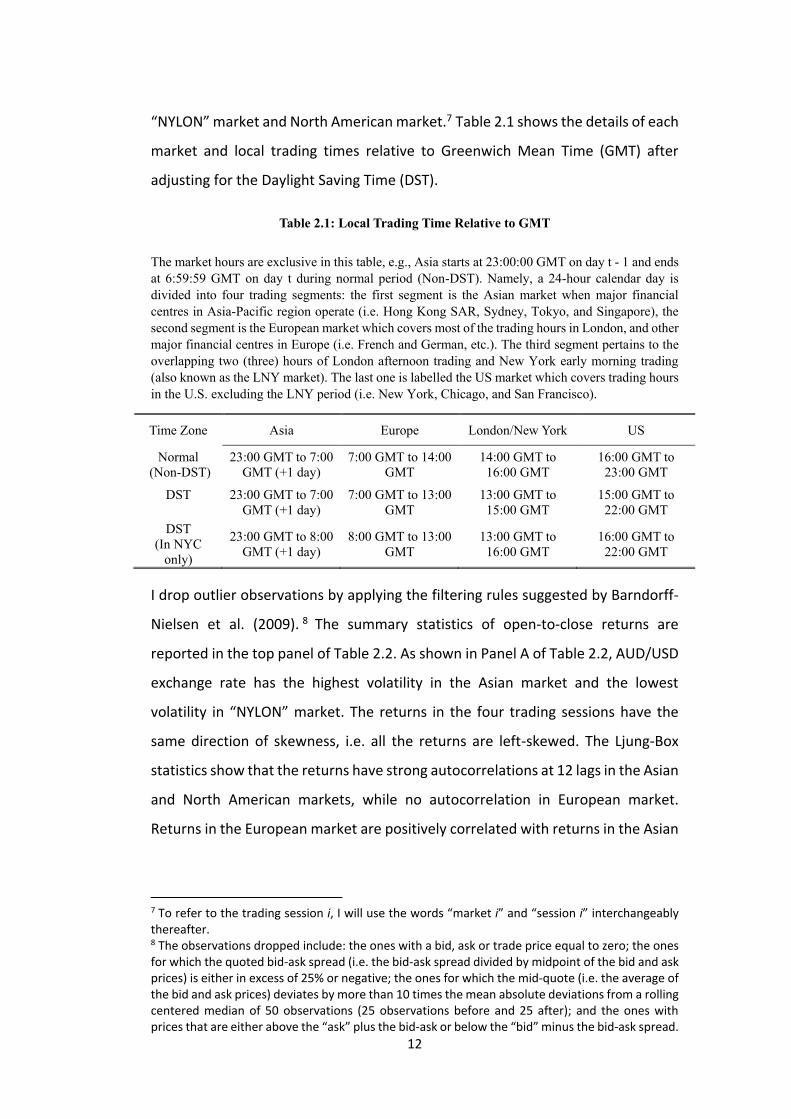
“NYLON” market and North American market.7 Table 2.1 shows the details of each

market and local trading times relative to Greenwich Mean Time (GMT) after

adjusting for the Daylight Saving Time (DST).

Table 2.1: Local Trading Time Relative to GMT

The market hours are exclusive in this table, e.g., Asia starts at 23:00:00 GMT on day t - 1 and ends

at 6:59:59 GMT on day t during normal period (Non-DST). Namely, a 24-hour calendar day is

divided into four trading segments: the first segment is the Asian market when major financial

centres in Asia-Pacific region operate (i.e. Hong Kong SAR, Sydney, Tokyo, and Singapore), the

second segment is the European market which covers most of the trading hours in London, and other

major financial centres in Europe (i.e. French and German, etc.). The third segment pertains to the

overlapping two (three) hours of London afternoon trading and New York early morning trading

(also known as the LNY market). The last one is labelled the US market which covers trading hours

in the U.S. excluding the LNY period (i.e. New York, Chicago, and San Francisco).

Time Zone Asia Europe London/New York US

Normal

(Non-DST)

23:00 GMT to 7:00

GMT (+1 day)

7:00 GMT to 14:00

GMT

14:00 GMT to

16:00 GMT

16:00 GMT to

23:00 GMT

DST

23:00 GMT to 7:00

GMT (+1 day)

7:00 GMT to 13:00

GMT

13:00 GMT to

15:00 GMT

15:00 GMT to

22:00 GMT

DST

(In NYC

only)

23:00 GMT to 8:00

GMT (+1 day)

8:00 GMT to 13:00

GMT

13:00 GMT to

16:00 GMT

16:00 GMT to

22:00 GMT

I drop outlier observations by applying the filtering rules suggested by Barndorff-

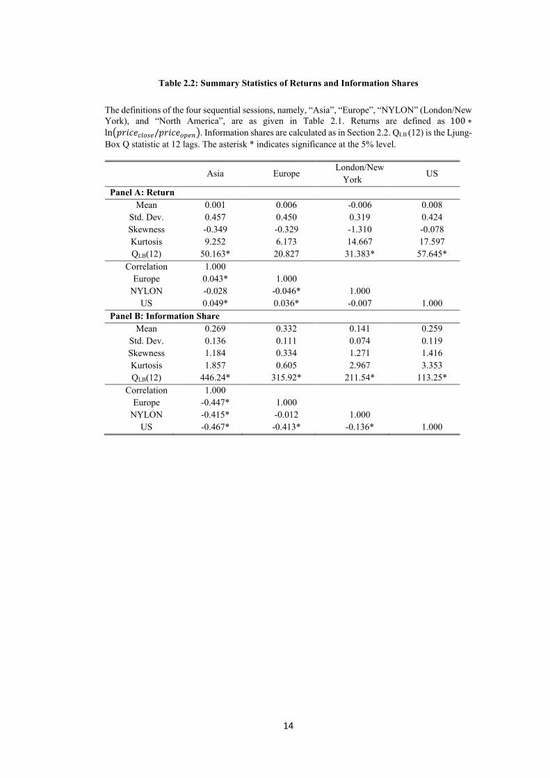
Nielsen et al. (2009). 8 The summary statistics of open-to-close returns are

reported in the top panel of Table 2.2. As shown in Panel A of Table 2.2, AUD/USD

exchange rate has the highest volatility in the Asian market and the lowest

volatility in “NYLON” market. The returns in the four trading sessions have the

same direction of skewness, i.e. all the returns are left-skewed. The Ljung-Box

statistics show that the returns have strong autocorrelations at 12 lags in the Asian

and North American markets, while no autocorrelation in European market.

Returns in the European market are positively correlated with returns in the Asian

7 To refer to the trading session i, I will use the words “market i” and “session i” interchangeably thereafter. 8 The observations dropped include: the ones with a bid, ask or trade price equal to zero; the ones for which the quoted bid-ask spread (i.e. the bid-ask spread divided by midpoint of the bid and ask prices) is either in excess of 25% or negative; the ones for which the mid-quote (i.e. the average of the bid and ask prices) deviates by more than 10 times the mean absolute deviations from a rolling centered median of 50 observations (25 observations before and 25 after); and the ones with prices that are either above the “ask” plus the bid-ask or below the “bid” minus the bid-ask spread.

13

and North American markets and negatively correlated with returns in “NYLON”

market.

Intraday returns at high frequency (i.e., 1-second) and low frequency (i.e., 5-

minute) intervals are computed in order to calculate the TSRV as discussed in

Section 2.1. I construct the mid-quote price as the average of bid and ask quotes

at the end of each sampling interval or the last observation of bid and ask quotes

prior to the end of an interval. The intraday return 𝑟𝑖,𝑡 is then calculated as 100

times the log ratio of the mid-quotes at times t and t-1, that is, 𝑟𝑖,𝑡 = 100 ∗

𝑙𝑛(𝑝𝑖,𝑡/𝑝𝑖,𝑡−1) . Panel B of Table 2.2 reports the summary statistics of the daily

information shares measured by the ratio of TSRV in market i to the daily TSRV on

a specific day. In the four markets, Europe has the largest average information

share, followed by North America, Asia, and “NYLON”. The information share in

Asia has the largest standard deviation as well as the strongest autocorrelation at

lag 12. Besides, all the information shares in four markets are negatively correlated.

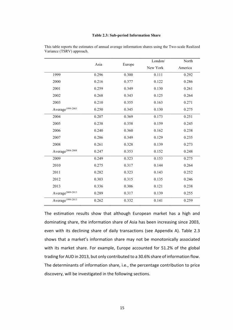
The yearly average information share of the four markets are reported in Table

2.3. It is interesting to note that if the 24 hours are divided into three 8-hour time

zones, then the European market, which includes the Europe and “NYLON” market,

dominates price discovery in AUD market. The combined information shares of

Europe and “NYLON” range from 44% to 54%, of which “NYLON” market (i.e. the

two- to three-hour overlapping trading session) accounts for a significant

proportion of price discovery in most years.

14

Table 2.2: Summary Statistics of Returns and Information Shares

The definitions of the four sequential sessions, namely, “Asia”, “Europe”, “NYLON” (London/New

York), and “North America”, are as given in Table 2.1. Returns are defined as 100 ∗

ln(𝑝𝑟𝑖𝑐𝑒𝑐𝑙𝑜𝑠𝑒/𝑝𝑟𝑖𝑐𝑒𝑜𝑝𝑒𝑛). Information shares are calculated as in Section 2.2. QLB (12) is the Ljung-

Box Q statistic at 12 lags. The asterisk * indicates significance at the 5% level.

Asia Europe London/New

York US

Panel A: Return

Mean 0.001 0.006 -0.006 0.008

Std. Dev. 0.457 0.450 0.319 0.424

Skewness -0.349 -0.329 -1.310 -0.078

Kurtosis 9.252 6.173 14.667 17.597

QLB(12) 50.163* 20.827 31.383* 57.645*

Correlation 1.000

Europe 0.043* 1.000

NYLON -0.028 -0.046* 1.000

US 0.049* 0.036* -0.007 1.000

Panel B: Information Share

Mean 0.269 0.332 0.141 0.259

Std. Dev. 0.136 0.111 0.074 0.119

Skewness 1.184 0.334 1.271 1.416

Kurtosis 1.857 0.605 2.967 3.353

QLB(12) 446.24* 315.92* 211.54* 113.25*

Correlation 1.000

Europe -0.447* 1.000

NYLON -0.415* -0.012 1.000

US -0.467* -0.413* -0.136* 1.000

15

Table 2.3: Sub-period Information Share

This table reports the estimates of annual average information shares using the Two-scale Realized

Variance (TSRV) approach.

Asia Europe London/

New York

North

America

1999 0.296 0.300 0.111 0.292

2000 0.216 0.377 0.122 0.286

2001 0.259 0.349 0.130 0.261

2002 0.268 0.343 0.125 0.264

2003 0.210 0.355 0.163 0.271

Average1999-2003 0.250 0.345 0.130 0.275

2004 0.207 0.369 0.173 0.251

2005 0.238 0.358 0.159 0.245

2006 0.240 0.360 0.162 0.238

2007 0.286 0.349 0.129 0.235

2008 0.261 0.328 0.139 0.273

Average2004-2008 0.247 0.353 0.152 0.248

2009 0.249 0.323 0.153 0.275

2010 0.275 0.317 0.144 0.264

2011 0.282 0.323 0.143 0.252

2012 0.303 0.315 0.135 0.246

2013 0.336 0.306 0.121 0.238

Average2009-2013 0.289 0.317 0.139 0.255

Average1999-2013 0.262 0.332 0.141 0.259

The estimation results show that although European market has a high and

dominating share, the information share of Asia has been increasing since 2003,

even with its declining share of daily transactions (see Appendix A). Table 2.3

shows that a market’s information share may not be monotonically associated

with its market share. For example, Europe accounted for 51.2% of the global

trading for AUD in 2013, but only contributed to a 30.6% share of information flow.

The determinants of information share, i.e., the percentage contribution to price

discovery, will be investigated in the following sections.

16

2.3. Determinants of price discovery: hypothesis formulation

Following the estimation of the information shares in different markets for AUD

trading, I turn to examining the determinants of price discovery in AUD market. In

this section, the hypotheses on the determinants of price discovery in AUD market

are discussed.

2.3.1. Market state-related variables

The existing studies have shown that information shares vary considerably across

different markets and the shares are also subject to instabilities arising from

different market states. The market states variables include bid-ask spread,

trading volume, and volatility (see, Brandt, Kavajecz and Underwood, 2007;

Mizrach and Neely, 2008), as well as the exchange rate return. Analysis of the

market state variables can also help us to identify the unconditional information

shares. Mizrach and Neely (2008), who are the first ones to systemically explore

the roles of market state variables, show that the bid-ask spread, traded contracts,

and volatility can explain the price discovery shifts between the US Treasury spot

and futures markets. Fricke and Menkhoff (2011) use market state variables to

examine the level of competition in price discovery among Euro bond futures with

different maturities. In this chapter I use three market state variables: (i) spread,

(ii) volume, and (iii) volatility. Moreover, I also consider the impact of exchange

rate return on the price discovery (i.e., whether the information share of a specific

market is higher on days with larger returns and vice versa).

Based on Mizrach and Neely (2008), I expect that a high bid-ask spread increases

the price of incorporating the private information, which in turn impedes the price

discovery process. However, Patel et al. (2014) find that higher information shares

of options are associated with wider options spreads, which can be explained by

the adverse selection risks faced by inter-bank market dealers (Kyle, 1985).9 In

contrast, a higher share of trading volume indicates more informed trading– or at

9 For example, with the presence of informed traders, the dealer would widen the bid-ask spread to reduce the adverse selection costs.

17

least, facilitates information processing – and thus increases the information share.

Besides, higher returns may help attract more trading activity, especially the

speculative trading, and thereby facilitate the information flows. Finally, the

impact of volatility is ambiguous: high volatility may be seen as an indicator of the

presence of the noise traders in the market and hence volatility decreases the

information share. However, volatility can also be a sign of heterogeneously

distributed information processing, which is expected to have a positive

relationship with market information share (Fricke and Menkhoff, 2011). In overall

terms, the evidence suggests that market state variables are important but their

expected effect on information shares is less obvious ex ante (see, for example,

Fricke and Menkhoff, 2011). Based on the above discussions, the following

hypothesis can be formulated:

Hypothesis 1: Market state-related variables have significant impacts on the

information shares for trading of AUD.

2.3.2. Macroeconomic news announcements

Among all the factors that influence price discovery, the impact of macroeconomic

news announcements has received special attention. Moshirian, Nguyen and

Pham (2012) argue that public information is crucial for the efficient functioning

of the capital market. The earliest studies of announcement effects on the foreign

exchange market constrained their consideration to the level changes of exchange

rates. However, since 1990s researchers have paid more attention to the

announcement effects on volatility. For example, Engle, Ito and Lin (1990)

introduce the concepts of the heat waves and meteor showers effects to explore

the links between intraday volatility pattern and macroeconomic news

announcements in the foreign exchange market.10 Andersen and Bollerslev (1998)

conjecture that the intraday volatility patterns alter daily trading patterns and the

US announcements are helpful in explaining volatility movements in Deutsche

10Heat waves refer to the idea that most important news that affects volatility and price discovery occurs during a particular session’s trading hours and there is little price discovery when that market is closed. In contrast, meteor showers pertain to the idea that information flow spills over across sessions, i.e., from Asia to Europe, then to the U.S. (Engle, et al., 1990).

18

Mark (DEM)/USD spot rate. Upper and Werner (2002) show that more information

is incorporated in the German bonds futures market during the announcement

periods and the contribution of the spot market to the common efficient price

varies in the range of 19-33%. Mizrach and Neely (2008) find that the release of

macroeconomic news weakens the importance of the German bond spot prices

compared to the futures prices. Andersen, Bollerslev, and Diebold (2007) detect

strong but short-lived news-effects on the 5-year bond futures contracts in an

international context. In the FX microstructure study, it is widely accepted that

information arrival typically does increase volatility (Melvin and Yin, 2000) and

news might create order flows that transmit private information to the FX market

(Dominguez and Panthaki, 2006). Recently, Gau and Wu (2017) utilize the same

method of TSRV ratio to study macroeconomic news announcements and price

discovery in the FX markets. The empirical results suggest that the dominant role

of the overlapping trading hours of LNY market in the price discovery of the EUR

and JPY markets only applies on days with U.S. announcements.

In this chapter, I use a wider set of macroeconomic news types compared to the

previous studies and examine whether this set of macroeconomic news affects the

price discovery process differently from the previous studies. For example, Evans

(2002) decompose macro news into common knowledge and non-common

knowledge shocks and find that non-common knowledge shocks are of greater

importance in price discovery. In the Bloomberg news dataset, most Australian

macroeconomic announcements arrive during the Asian trading hours (i.e. from

23:00 GMT on day t-1 to 1:00 GMT on day t), while most of the US macroeconomic

announcements occur during the “NYLON” and North American markets (i.e., from

12:00 GMT to 19:00 GMT). In order to investigate whether macroeconomics news

releases during the trading hours affect the specific trading session’s price

discovery process, I compare the average information shares of the trading

sessions on announcement days versus non-announcement days. As shown in

Table 2.4, on the Australian macroeconomic news announcement days, the

information share of Asia increases significantly, whereas those of the European

and North American markets decline. In contrast, on the US-related

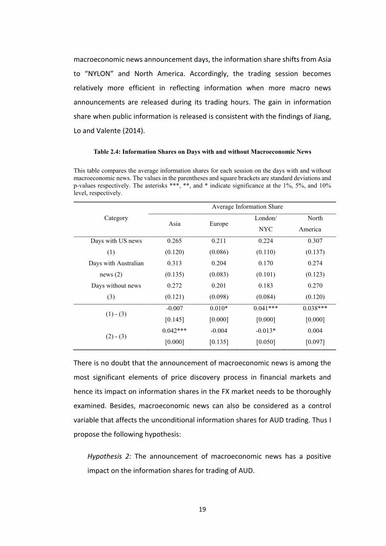
19

macroeconomic news announcement days, the information share shifts from Asia

to “NYLON” and North America. Accordingly, the trading session becomes

relatively more efficient in reflecting information when more macro news

announcements are released during its trading hours. The gain in information

share when public information is released is consistent with the findings of Jiang,

Lo and Valente (2014).

Table 2.4: Information Shares on Days with and without Macroeconomic News

This table compares the average information shares for each session on the days with and without

macroeconomic news. The values in the parentheses and square brackets are standard deviations and

p-values respectively. The asterisks ***, **, and * indicate significance at the 1%, 5%, and 10%

level, respectively.

Category

Average Information Share

Asia Europe London/

NYC

North

America

Days with US news

(1)

0.265

(0.120)

0.211

(0.086)

0.224

(0.110)

0.307

(0.137)

Days with Australian

news (2)

0.313

(0.135)

0.204

(0.083)

0.170

(0.101)

0.274

(0.123)

Days without news

(3)

0.272

(0.121)

0.201

(0.098)

0.183

(0.084)

0.270

(0.120)

(1) - (3) -0.007

[0.145]

0.010*

[0.000]

0.041***

[0.000]

0.038***

[0.000]

(2) - (3) 0.042***

[0.000]

-0.004

[0.135]

-0.013*

[0.050]

0.004

[0.097]

There is no doubt that the announcement of macroeconomic news is among the

most significant elements of price discovery process in financial markets and

hence its impact on information shares in the FX market needs to be thoroughly

examined. Besides, macroeconomic news can also be considered as a control

variable that affects the unconditional information shares for AUD trading. Thus I

propose the following hypothesis:

Hypothesis 2: The announcement of macroeconomic news has a positive

impact on the information shares for trading of AUD.

20

2.3.3. Order flows

Order flow is a measure of the signed trades and calculated as the difference

between buy- and sell-initiated trades over a particular market (assuming that

buys are coded positive). It is well documented that order flow is positively related

to contemporaneous returns in many financial markets.11 This is often interpreted

as an indication of order flow being the medium for incorporating information into

prices. In microstructure studies, it has been argued that private information is

embedded in the prices via order flows. For example, Evans and Lyons (1999)

argue that order flow is a crucial determinant of the price in microstructure models

that aim to explain exchange rate fluctuations. Using a microstructure model,

Killeen, Lyons and Moore (2006) show that shocks to order flow induce more

volatility under flexible exchange rates. Evans and Lyons (2008) confirm that up to

two thirds of the level changes and volatilities in exchange rate movements are

associated with order flows.

However, it has been suggested that order flow may contain elements that are not

related to information. For example, in practice, the momentum trading strategy

may generate a large amount of order flows that are unrelated to information.

Pasquariello and Vega (2007) suggest a new approach that allows one to extract

the truly informative part of order flow. They highlight a linkage between

unexpected order flow and information processing in the bond market. In addition,

Chai et al. (2015) examine the information distribution in the global gold market

and adopt the unexpected order flow as a proxy for private information.

Furthermore, Green (2004) emphasize the processing of public news via order

flows. Namely, the order flow can impact price discovery and its information effect

varies across the days with and without news. Based on the existing studies, the

hypotheses 3.1 and 3.2 can be specified as follows:

11 In this study, the Pearson correlations among the market state variables and order flow also suggest that order flow is significantly and positively correlated with contemporaneous returns. The results are not presented here due to space constraints, but available upon request.

21

Hypothesis 3.1: Order flow has a positive impact on the information shares for

trading of AUD.

Hypothesis 3.2: On macroeconomic news release days, order flow has a more

significantly positive impact on the information shares for trading of AUD.

2.3.4. Cross-market information flow and dynamic structure

Some relevant studies, such as Evans and Lyons (2002), suggested the possibility

of the cross-market information flows, that is, the information flow of a currency

could be correlated to those of other currencies. Unlike Evans and Lyons (2002)

focusing on different currencies, I conjecture that the cross-market effect exists

among different trading sessions of the same currency. In order to test the

existence of cross-market information spillover effect, I utilize the technique of

Shapley-Owen R2 decomposition, which can explicitly examine the relative

importance of each variable (i.e. the percentage contribution) in explaining the

dependent variable.12 Su and Wang (2017) measure the magnitudes of meteor

shower and heat waves effects (i.e. inter-regional and intra-regional volatility

spillovers respectively) in the FX market and find that the cross-market

information propagation has been increasing recently. Similarly, I conduct the

Shapley-Owen R2 decomposition for the HAR-IS model and find that the cross-

market effect on information spillover is significant and contributes to 58% of the

total variations in daily information share, while the local-market effect

constitutes the remaining portion. 13 Specifically, I extend the classic

heterogeneous autoregressive model (HAR) and regress the daily information

share of session i on the lagged daily, weekly, and monthly information shares of

its own-market and other markets respectively. The sum of incremental increase

in the model R2 resulting from the addition of a predictor, or set of predictors of

lagged own-market and other markets are local-market and cross-market effects

12 For a detailed introduction to the Shapley-Owen R2 decomposition and its applications, please refer to Lahaye and Neely (2016). 13 The HAR-class model which examines the short-run dependence of variable of interest while controlling for the longer-run dependence (i.e. weekly and monthly dependence) was firstly proposed by Corsi (2009) and has been widely used in the relevant literature (see, for example, Bollerslev et al., 2017; Su, 2017; among many others).

22

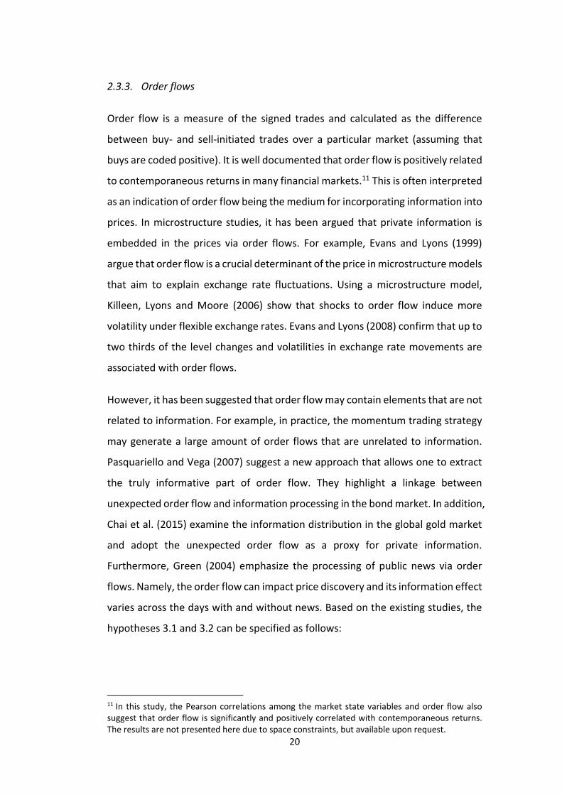
respectively. The results of the Shapley-Owen R2 decomposition are shown in

Table 2.5 as below:

Table 2.5: Shapley-Owen Values for the Local- and Cross-market Spillover Effect

This table shows the Shapley-Owen proportion of the total R2s in four trading sessions, for groups

of coefficients in the HAR model in which Information Share (IS) is predicted by lagged IS. There

are 2 groups of coefficients: The own-market contribution, which includes one day lagged IS, lagged

weekly and monthly information shares of its own market; as well as and the cross-market

contribution, which includes counterparts of lagged IS of other markets. The groups have no

intersection and include all non-deterministic regressors, so the proportions for each intraday period

sum to 100.

Furthermore, in order to test the possibility of self-dynamics, I plot the

autocorrelation functions (ACF) of the daily and monthly information shares for

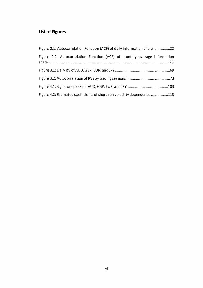
each trading session respectively. As shown in Figure 2.1, there are weak

autocorrelations in daily information shares, which confirms the strong daily

variations of the information share as suggested in the previous section.14

Figure 2.1: Autocorrelation Function (ACF) of Daily Information Share

14 The Augmented Dicky-Fuller (ADF) test rejects the null hypothesis of a unit root and suggests that all the log transformations of information shares are stationary.

-0.05

0

0.05

0.1

0.15

0.2

0.25

1 5 9

13

17

21

25

29

33

37

41

45

49

53

57

61

65

69

73

77

81

85

89

93

97

Lags

Aisa Europe LNY US

Asia Europe London/NYC North

America Average

local-market 0.40 0.43 0.39 0.45 0.42

cross-market 0.60 0.57 0.61 0.55 0.58

23

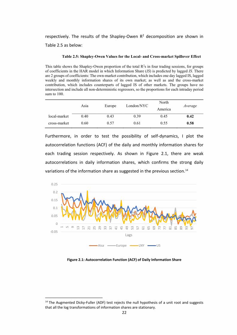
Slightly different results have been found for the ACF of the monthly average

information share of each trading session. For example, it suggests a slow-

decaying process for the monthly information share as shown in the figure below:

Figure 2.2: Autocorrelation Function (ACF) of Monthly Average Information Share

Based on the results of Shapley-Owen R2 decomposition and ACF analysis, the

hypotheses 4.1 and 4.2 can be proposed as follows:

Hypothesis 4.1: Cross-market information flow has an impact on the

information shares for trading of AUD.

Hypothesis 4.2: Self-dependence of information flow also has an impact on

the information shares for trading of AUD.

2.3.5. Long-run determinants of the information shares

The existing literature on market risks suggests that aggregate volatility is subject

to shocks at different frequencies (Adrian and Rosenberg, 2008). Following this

line of reasoning, I examine the determinants of information shares over a longer

time horizon (i.e. on a monthly basis). Specifically, following Sassen (1999) who

claim that the two most important factors in transforming a city into a global

financial centre are international consolidation of financial activities (i.e.,

concentration of financial institutions and transactions in one location) and

financial market liberalization (i.e., financial services openness and free capital

flows), I make an attempt to identify the key factors in determining the

“information hierarchy” in FX trading and conjecture that the financial market

0

0.2

0.4

0.6

0.8

1 2 3 4 5 6 7 8 9 10 11 12

Lags

Asia Europe LNY US

24

development and integration of a financial centre affects its price discovery

capability. Specifically, in this study, I utilize pricing efficiency as an indicator of the

financial market development. I also use the number of quoting banks (both local

and foreign banks) and concentration of transactions (i.e., the total market share

of top-5 most active quoting banks) as indicators of market consolidation, as well

as the Chinn-Ito index as a proxy for the degree of capital market openness and

financial market liberalization (Chinn and Ito, 2006). The last hypothesis is

organized as follows:

Hypothesis 5: Financial market development and integration of financial

centres also have positive impacts on the information shares for the AUD

trading in the long-run.

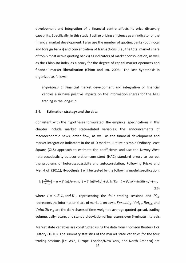
2.4. Estimation strategy and the data

Consistent with the hypotheses formulated, the empirical specifications in this

chapter include market state-related variables, the announcements of

macroeconomic news, order flow, as well as the financial development and

market integration indicators in the AUD market. I utilize a simple Ordinary Least

Square (OLS) approach to estimate the coefficients and use the Newey-West

heteroscedasticity-autocorrelation-consistent (HAC) standard errors to correct

the problems of heteroscedasticity and autocorrelation. Following Fricke and

Menkhoff (2011), Hypothesis 1 will be tested by the following model specification:

ln (𝐼𝑆𝑖.𝑡

1−𝐼𝑆𝑖.𝑡) = 𝛼 + 𝛽1 ln(𝑆𝑝𝑟𝑒𝑎𝑑𝑖.𝑡) + 𝛽2 ln(𝑉𝑜𝑙𝑖.𝑡) + 𝛽3 ln(𝑅𝑒𝑡𝑖.𝑡) + 𝛽4 ln(𝑉𝑜𝑙𝑎𝑡𝑖𝑙𝑖𝑡𝑦𝑖.𝑡) + 𝜖𝑖,𝑡

(2.3)

where 𝑖 = 𝐴, 𝐸, 𝐿, 𝑎𝑛𝑑 𝑈 , representing the four trading sessions and 𝐼𝑆𝑖.𝑡

represents the information share of market i on day t. 𝑆𝑝𝑟𝑒𝑎𝑑𝑖,𝑡, 𝑉𝑜𝑙𝑖,𝑡, 𝑅𝑒𝑡𝑖.𝑡, and

𝑉𝑜𝑙𝑎𝑡𝑖𝑙𝑖𝑡𝑦𝑖.𝑡 are the daily shares of time-weighted average quoted spread, trading

volume, daily return, and standard deviation of log returns over 5-minute intervals.

Market state variables are constructed using the data from Thomson Reuters Tick

History (TRTH). The summary statistics of the market state variables for the four

trading sessions (i.e. Asia, Europe, London/New York, and North America) are

25

provided in Panel A of Appendix B. The Ljung-Box Q statistics show that the

volatility has strong autocorrelations in Asian, European, and North American

markets, while it shows no autocorrelation for “NYLON” market. The Augmented

Dicky-Fuller (ADF) tests suggest that the daily shares of all market state variables

are stationary, i.e. all the series expressed as percentage shares are I(0) processes

and hence simple regression can be used for hypothesis testing.

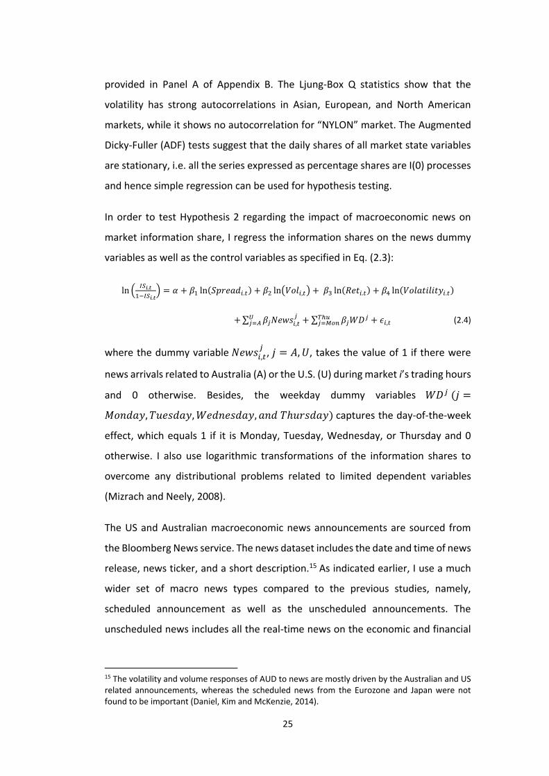
In order to test Hypothesis 2 regarding the impact of macroeconomic news on

market information share, I regress the information shares on the news dummy

variables as well as the control variables as specified in Eq. (2.3):


1−𝐼𝑆𝑖.𝑡) = 𝛼 + 𝛽1 ln(𝑆𝑝𝑟𝑒𝑎𝑑𝑖.𝑡) + 𝛽2 ln(𝑉𝑜𝑙𝑖,𝑡) + 𝛽3 ln(𝑅𝑒𝑡𝑖.𝑡) + 𝛽4 ln(𝑉𝑜𝑙𝑎𝑡𝑖𝑙𝑖𝑡𝑦𝑖.𝑡)

+ ∑ 𝛽𝑗𝑁𝑒𝑤𝑠𝑖,𝑡𝑗𝑈

𝑗=𝐴 + ∑ 𝛽𝑗𝑊𝐷𝑗𝑇ℎ𝑢𝑗=𝑀𝑜𝑛 + 𝜖𝑖,𝑡 (2.4)

where the dummy variable 𝑁𝑒𝑤𝑠𝑖,𝑡𝑗

, 𝑗 = 𝐴, 𝑈, takes the value of 1 if there were

news arrivals related to Australia (A) or the U.S. (U) during market i’s trading hours

and 0 otherwise. Besides, the weekday dummy variables 𝑊𝐷𝑗 (𝑗 =

𝑀𝑜𝑛𝑑𝑎𝑦, 𝑇𝑢𝑒𝑠𝑑𝑎𝑦, 𝑊𝑒𝑑𝑛𝑒𝑠𝑑𝑎𝑦, 𝑎𝑛𝑑 𝑇ℎ𝑢𝑟𝑠𝑑𝑎𝑦) captures the day-of-the-week

effect, which equals 1 if it is Monday, Tuesday, Wednesday, or Thursday and 0

otherwise. I also use logarithmic transformations of the information shares to

overcome any distributional problems related to limited dependent variables

(Mizrach and Neely, 2008).

The US and Australian macroeconomic news announcements are sourced from

the Bloomberg News service. The news dataset includes the date and time of news

release, news ticker, and a short description.15 As indicated earlier, I use a much

wider set of macro news types compared to the previous studies, namely,

scheduled announcement as well as the unscheduled announcements. The

unscheduled news includes all the real-time news on the economic and financial

15 The volatility and volume responses of AUD to news are mostly driven by the Australian and US related announcements, whereas the scheduled news from the Eurozone and Japan were not found to be important (Daniel, Kim and McKenzie, 2014).

26

markets of Australia and the U.S. as well as key international market-moving

headlines.

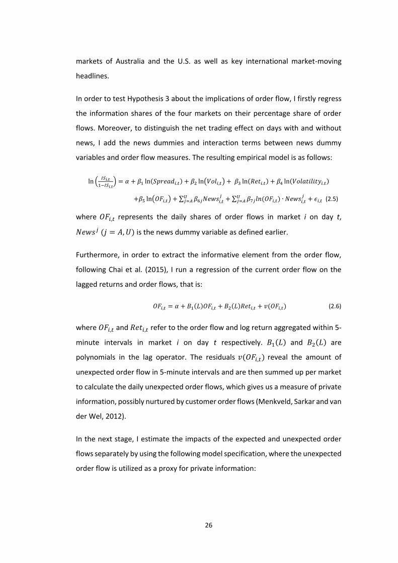
In order to test Hypothesis 3 about the implications of order flow, I firstly regress

the information shares of the four markets on their percentage share of order

flows. Moreover, to distinguish the net trading effect on days with and without

news, I add the news dummies and interaction terms between news dummy

variables and order flow measures. The resulting empirical model is as follows:



+𝛽5 ln(𝑂𝐹𝑖,𝑡) + ∑ 𝛽6𝑗𝑁𝑒𝑤𝑠𝑖,𝑡𝑗𝑈

𝑗=𝐴 + ∑ 𝛽7𝑗𝑙𝑛 (𝑂𝐹𝑖,𝑡) ∙ 𝑁𝑒𝑤𝑠𝑖,𝑡𝑗𝑈

𝑗=𝐴 + 𝜖𝑖,𝑡 (2.5)

where 𝑂𝐹𝑖,𝑡 represents the daily shares of order flows in market i on day t,

𝑁𝑒𝑤𝑠𝑗 (𝑗 = 𝐴, 𝑈) is the news dummy variable as defined earlier.

Furthermore, in order to extract the informative element from the order flow,

following Chai et al. (2015), I run a regression of the current order flow on the

lagged returns and order flows, that is:

𝑂𝐹𝑖,𝑡 = 𝛼 + 𝐵1(𝐿)𝑂𝐹𝑖,𝑡 + 𝐵2(𝐿)𝑅𝑒𝑡𝑖,𝑡 + 𝑣(𝑂𝐹𝑖,𝑡) (2.6)

where 𝑂𝐹𝑖,𝑡 and 𝑅𝑒𝑡𝑖,𝑡 refer to the order flow and log return aggregated within 5-

minute intervals in market i on day t respectively. 𝐵1(𝐿) and 𝐵2(𝐿) are

polynomials in the lag operator. The residuals 𝑣(𝑂𝐹𝑖,𝑡) reveal the amount of

unexpected order flow in 5-minute intervals and are then summed up per market

to calculate the daily unexpected order flows, which gives us a measure of private

information, possibly nurtured by customer order flows (Menkveld, Sarkar and van

der Wel, 2012).

In the next stage, I estimate the impacts of the expected and unexpected order

flows separately by using the following model specification, where the unexpected

order flow is utilized as a proxy for private information:

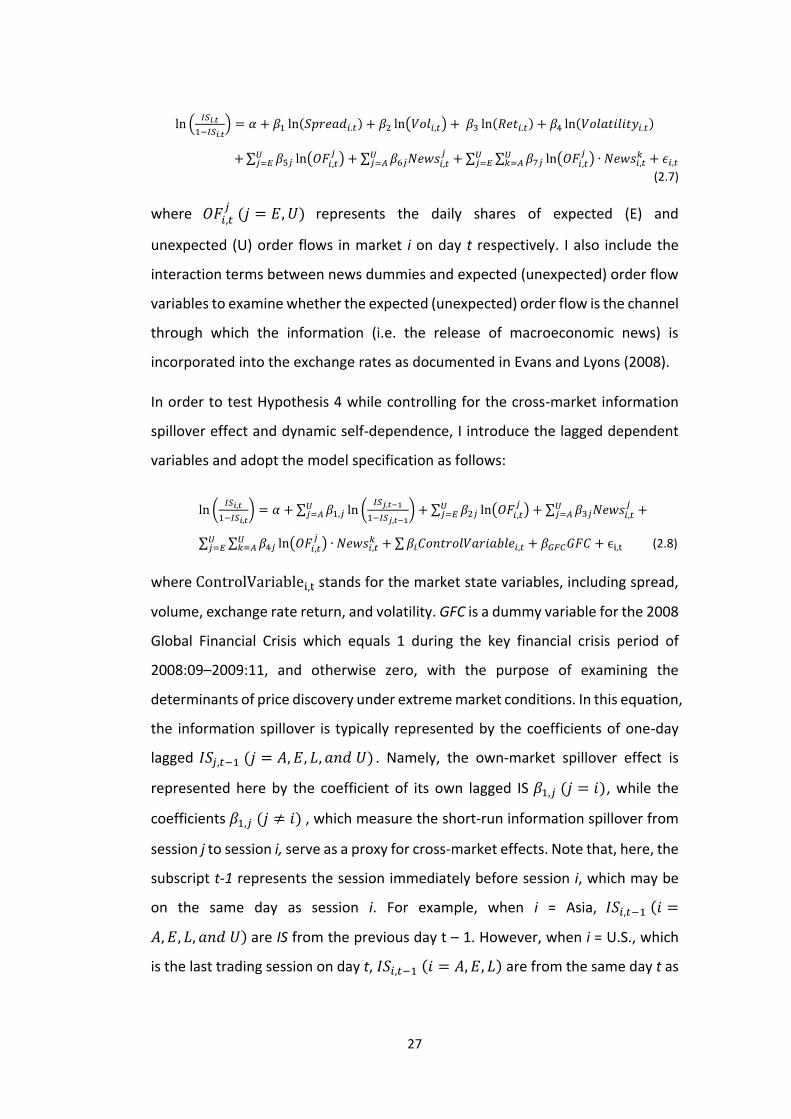
27



+ ∑ 𝛽5𝑗 ln(𝑂𝐹𝑖,𝑡𝑗

)𝑈𝑗=𝐸 + ∑ 𝛽6𝑗𝑁𝑒𝑤𝑠𝑖,𝑡

𝑗𝑈𝑗=𝐴 + ∑ ∑ 𝛽7𝑗 ln(𝑂𝐹𝑖,𝑡

𝑗) ∙ 𝑁𝑒𝑤𝑠𝑖,𝑡

𝑘𝑈𝑘=𝐴

𝑈𝑗=𝐸 + 𝜖𝑖,𝑡

(2.7)

where 𝑂𝐹𝑖,𝑡𝑗

(𝑗 = 𝐸, 𝑈) represents the daily shares of expected (E) and

unexpected (U) order flows in market i on day t respectively. I also include the

interaction terms between news dummies and expected (unexpected) order flow

variables to examine whether the expected (unexpected) order flow is the channel

through which the information (i.e. the release of macroeconomic news) is

incorporated into the exchange rates as documented in Evans and Lyons (2008).

In order to test Hypothesis 4 while controlling for the cross-market information

spillover effect and dynamic self-dependence, I introduce the lagged dependent

variables and adopt the model specification as follows:

ln (𝐼𝑆𝑖,𝑡

1−𝐼𝑆𝑖,𝑡) = 𝛼 + ∑ 𝛽1,𝑗 ln (

𝐼𝑆𝑗,𝑡−1

1−𝐼𝑆𝑗,𝑡−1)𝑈

𝑗=𝐴 + ∑ 𝛽2𝑗 ln(𝑂𝐹𝑖,𝑡𝑗


𝑗𝑈𝑗=𝐴 +

∑ ∑ 𝛽4𝑗 ln(𝑂𝐹𝑖,𝑡𝑗

) ∙ 𝑁𝑒𝑤𝑠𝑖,𝑡𝑘 + ∑ 𝛽𝑖𝐶𝑜𝑛𝑡𝑟𝑜𝑙𝑉𝑎𝑟𝑖𝑎𝑏𝑙𝑒𝑖,𝑡 + 𝛽𝐺𝐹𝐶𝐺𝐹𝐶 + ϵi,t

𝑈𝑘=𝐴

𝑈𝑗=𝐸 (2.8)

where ControlVariablei,t stands for the market state variables, including spread,

volume, exchange rate return, and volatility. GFC is a dummy variable for the 2008

Global Financial Crisis which equals 1 during the key financial crisis period of

2008:09–2009:11, and otherwise zero, with the purpose of examining the

determinants of price discovery under extreme market conditions. In this equation,

the information spillover is typically represented by the coefficients of one-day

lagged 𝐼𝑆𝑗,𝑡−1 (𝑗 = 𝐴, 𝐸, 𝐿, 𝑎𝑛𝑑 𝑈) . Namely, the own-market spillover effect is

represented here by the coefficient of its own lagged IS 𝛽1,𝑗 (𝑗 = 𝑖), while the

coefficients 𝛽1,𝑗 (𝑗 ≠ 𝑖) , which measure the short-run information spillover from

session j to session i, serve as a proxy for cross-market effects. Note that, here, the

subscript t-1 represents the session immediately before session i, which may be

on the same day as session i. For example, when i = Asia, 𝐼𝑆𝑖,𝑡−1 (𝑖 =

𝐴, 𝐸, 𝐿, 𝑎𝑛𝑑 𝑈) are IS from the previous day t – 1. However, when i = U.S., which

is the last trading session on day t, 𝐼𝑆𝑖,𝑡−1 (𝑖 = 𝐴, 𝐸, 𝐿) are from the same day t as

28

US market with only the lagged U.S. information share 𝐼𝑆𝑖,𝑡−1 (𝑖 = 𝑈) from the

previous day.

While the definition of Two-scale estimator pertains to the daily variance measure,

the volatility over longer horizons, say, weekly or monthly, may similarly be

estimated by summing the intraday squared changes of efficient price over a week

or a month. Thus, from a practical perspective, the approach of realized variance

parsimoniously captures the shocks at different horizons (Bollerslev et al., 2017).

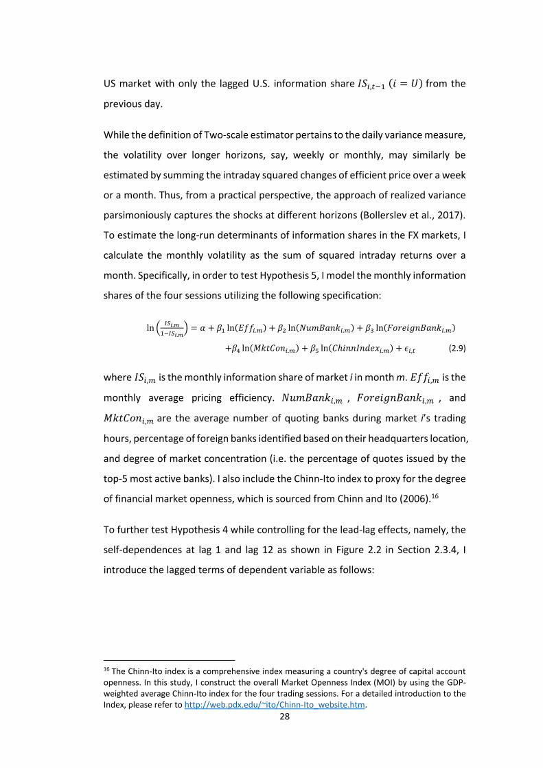
To estimate the long-run determinants of information shares in the FX markets, I

calculate the monthly volatility as the sum of squared intraday returns over a

month. Specifically, in order to test Hypothesis 5, I model the monthly information

shares of the four sessions utilizing the following specification:

ln (𝐼𝑆𝑖.𝑚

1−𝐼𝑆𝑖.𝑚) = 𝛼 + 𝛽1 ln(𝐸𝑓𝑓𝑖.𝑚) + 𝛽2 ln(𝑁𝑢𝑚𝐵𝑎𝑛𝑘𝑖.𝑚) + 𝛽3 ln(𝐹𝑜𝑟𝑒𝑖𝑔𝑛𝐵𝑎𝑛𝑘𝑖.𝑚)

+𝛽4 ln(𝑀𝑘𝑡𝐶𝑜𝑛𝑖.𝑚) + 𝛽5 ln(𝐶ℎ𝑖𝑛𝑛𝐼𝑛𝑑𝑒𝑥𝑖.𝑚) + 𝜖𝑖,𝑡 (2.9)

where 𝐼𝑆𝑖,𝑚 is the monthly information share of market i in month m. 𝐸𝑓𝑓𝑖,𝑚 is the

monthly average pricing efficiency. 𝑁𝑢𝑚𝐵𝑎𝑛𝑘𝑖,𝑚 , 𝐹𝑜𝑟𝑒𝑖𝑔𝑛𝐵𝑎𝑛𝑘𝑖,𝑚 , and

𝑀𝑘𝑡𝐶𝑜𝑛𝑖,𝑚 are the average number of quoting banks during market i’s trading

hours, percentage of foreign banks identified based on their headquarters location,

and degree of market concentration (i.e. the percentage of quotes issued by the

top-5 most active banks). I also include the Chinn-Ito index to proxy for the degree

of financial market openness, which is sourced from Chinn and Ito (2006).16

To further test Hypothesis 4 while controlling for the lead-lag effects, namely, the

self-dependences at lag 1 and lag 12 as shown in Figure 2.2 in Section 2.3.4, I

introduce the lagged terms of dependent variable as follows:

16 The Chinn-Ito index is a comprehensive index measuring a country's degree of capital account openness. In this study, I construct the overall Market Openness Index (MOI) by using the GDP-weighted average Chinn-Ito index for the four trading sessions. For a detailed introduction to the Index, please refer to http://web.pdx.edu/~ito/Chinn-Ito_website.htm.

http://web.pdx.edu/~ito/Chinn-Ito_website.htm

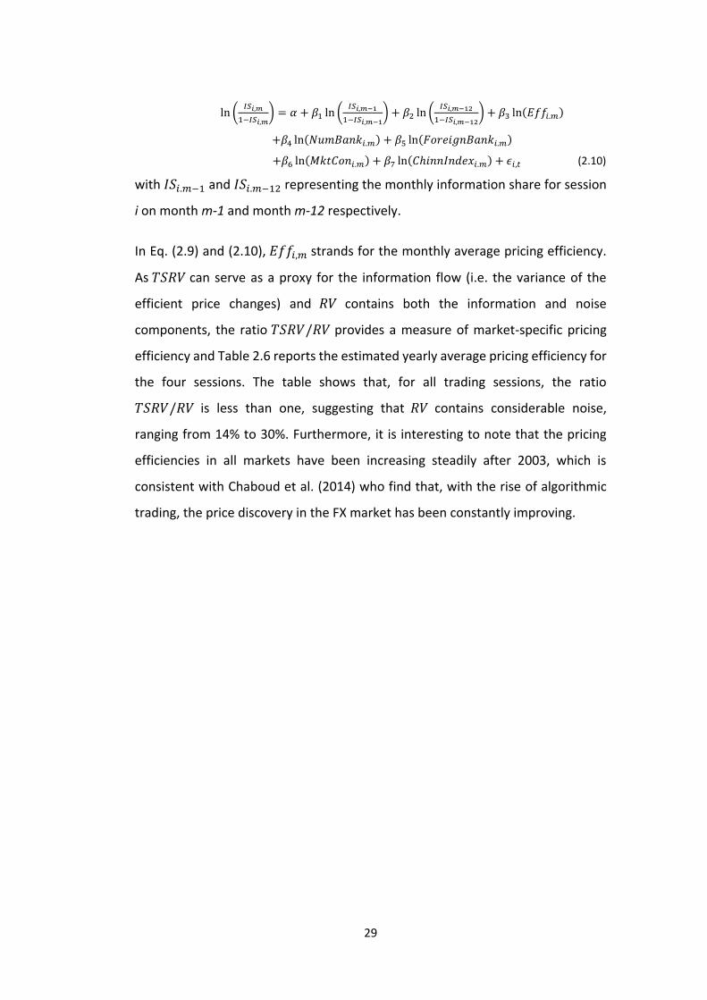
29

ln (𝐼𝑆𝑖,𝑚

1−𝐼𝑆𝑖,𝑚) = 𝛼 + 𝛽1 ln (

𝐼𝑆𝑖,𝑚−1

1−𝐼𝑆𝑖,𝑚−1) + 𝛽2 ln (


1−𝐼𝑆𝑖,𝑚−12) + 𝛽3 ln(𝐸𝑓𝑓𝑖.𝑚)

+𝛽4 ln(𝑁𝑢𝑚𝐵𝑎𝑛𝑘𝑖.𝑚) + 𝛽5 ln(𝐹𝑜𝑟𝑒𝑖𝑔𝑛𝐵𝑎𝑛𝑘𝑖.𝑚)

+𝛽6 ln(𝑀𝑘𝑡𝐶𝑜𝑛𝑖.𝑚) + 𝛽7 ln(𝐶ℎ𝑖𝑛𝑛𝐼𝑛𝑑𝑒𝑥𝑖.𝑚) + 𝜖𝑖,𝑡 (2.10)

with 𝐼𝑆𝑖.𝑚−1 and 𝐼𝑆𝑖.𝑚−12 representing the monthly information share for session

i on month m-1 and month m-12 respectively.

In Eq. (2.9) and (2.10), 𝐸𝑓𝑓𝑖,𝑚 strands for the monthly average pricing efficiency.

As 𝑇𝑆𝑅𝑉 can serve as a proxy for the information flow (i.e. the variance of the

efficient price changes) and 𝑅𝑉 contains both the information and noise

components, the ratio 𝑇𝑆𝑅𝑉/𝑅𝑉 provides a measure of market-specific pricing

efficiency and Table 2.6 reports the estimated yearly average pricing efficiency for

the four sessions. The table shows that, for all trading sessions, the ratio

𝑇𝑆𝑅𝑉/𝑅𝑉 is less than one, suggesting that 𝑅𝑉 contains considerable noise,

ranging from 14% to 30%. Furthermore, it is interesting to note that the pricing

efficiencies in all markets have been increasing steadily after 2003, which is

consistent with Chaboud et al. (2014) who find that, with the rise of algorithmic

trading, the price discovery in the FX market has been constantly improving.

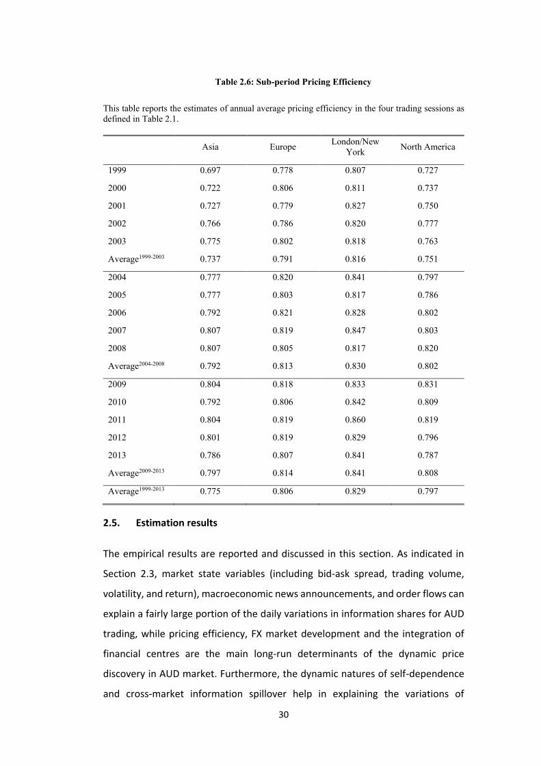
30

Table 2.6: Sub-period Pricing Efficiency

This table reports the estimates of annual average pricing efficiency in the four trading sessions as

defined in Table 2.1.


York North America

1999 0.697 0.778 0.807 0.727

2000 0.722 0.806 0.811 0.737

2001 0.727 0.779 0.827 0.750

2002 0.766 0.786 0.820 0.777

2003 0.775 0.802 0.818 0.763

Average1999-2003 0.737 0.791 0.816 0.751

2004 0.777 0.820 0.841 0.797

2005 0.777 0.803 0.817 0.786

2006 0.792 0.821 0.828 0.802

2007 0.807 0.819 0.847 0.803

2008 0.807 0.805 0.817 0.820

Average2004-2008 0.792 0.813 0.830 0.802

2009 0.804 0.818 0.833 0.831

2010 0.792 0.806 0.842 0.809

2011 0.804 0.819 0.860 0.819

2012 0.801 0.819 0.829 0.796

2013 0.786 0.807 0.841 0.787

Average2009-2013 0.797 0.814 0.841 0.808

Average1999-2013 0.775 0.806 0.829 0.797

2.5. Estimation results

The empirical results are reported and discussed in this section. As indicated in

Section 2.3, market state variables (including bid-ask spread, trading volume,

volatility, and return), macroeconomic news announcements, and order flows can

explain a fairly large portion of the daily variations in information shares for AUD

trading, while pricing efficiency, FX market development and the integration of

financial centres are the main long-run determinants of the dynamic price

discovery in AUD market. Furthermore, the dynamic natures of self-dependence

and cross-market information spillover help in explaining the variations of

31

information shares both in the short- and long-run. The results of robustness

testing are also presented in this section.

2.5.1. Market state variables

The estimation results regarding the market state variables are presented in Table

2.7. These results confirm that market state variables explain a significant

proportion of the fluctuations in the information shares in AUD market. In overall

terms, the market state-related variables perform better in explaining the shifts in

the information shares of the Asian market compared to the other markets, i.e.,

the adjusted R-squared for Asian market is as high as 0.8. A positive change in the

trading volume increases the information content of all markets. Interestingly, in

general, increases in spreads alone do not indicate less information processing.

The reason could be that, larger spreads are generally associated with more

informed trading, which is consistent with the findings of Glosten and Milgrom

(1985) who argue that the presence of informed traders leads to larger bid-ask

spreads. However, it is worth noting that after controlling for volatility (i.e., the

standard deviation of exchange rate returns over 5-minute intervals), the sign of

spread changes from positive to negative except for the US market as shown in

column (2) of Table 4.7. This result could be attributed to the fact that the bid/ask

spread consists of three components, namely, the asymmetric information

component (AIC), order processing component (OPC), and inventory holding

component (IHC) (Lin, Sanger and Booth 1995). While the asymmetric information

component is positively related to the information share, the order processing and

inventory holding components are significantly negatively related to the

information share. Thus, after controlling for the asymmetric information as

proxied by the volatility, an inverse relationship between spread and information

share has been documented. In addition, the estimation results confirm that

higher returns have a positive effect on price discovery in the foreign exchange

market.

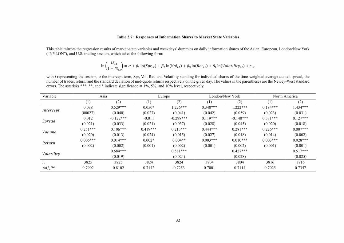
32

Table 2.7: Responses of Information Shares to Market State Variables

This table mirrors the regression results of market-state variables and weekdays’ dummies on daily information shares of the Asian, European, London/New York

(“NYLON”), and U.S. trading session, which takes the following form:


1 − 𝐼𝑆𝑖.𝑡) = 𝛼 + 𝛽1 ln(𝑆𝑝𝑟𝑖.𝑡) + 𝛽2 ln(𝑉𝑜𝑙𝑖.𝑡) + 𝛽3 ln(𝑅𝑒𝑡𝑖.𝑡) + 𝛽4 ln(𝑉𝑜𝑙𝑎𝑡𝑖𝑙𝑖𝑡𝑦𝑖.𝑡) + 𝜖𝑖,𝑡

with i representing the session, 𝛼 the intercept term, Spr, Vol, Ret, and Volatility standing for individual shares of the time-weighted average quoted spread, the

number of trades, return, and the standard deviation of mid-quote returns respectively on the given day. The values in the parentheses are the Newey-West standard

errors. The asterisks ***, **, and * indicate significance at 1%, 5%, and 10% level, respectively.

Variable Asia Europe London/New York North America

(1) (2) (1) (2) (1) (2) (1) (2)

𝐼𝑛𝑡𝑒𝑟𝑐𝑒𝑝𝑡 0.038

(00027)

0.529***

(0.040)

0.050*

(0.027)

1.226***

(0.041)

0.340***

(0.042)

1.222***

(0.059)

0.184***

(0.023)

1.434***

(0.031)

𝑆𝑝𝑟𝑒𝑎𝑑 0.012

(0.021)

-0.122***

(0.033)

-0.011

(0.021)

-0.298***

(0.037)

0.119***

(0.028)

-0.140***

(0.045)

0.531***

(0.020)

0.127***

(0.018)

𝑉𝑜𝑙𝑢𝑚𝑒 0.251***

(0.020)

0.106***

(0.013)

0.419***

(0.024)

0.213***

(0.015)

0.444***

(0.027)

0.281***

(0.018)

0.226***

(0.014)

0.007***

(0.002)

𝑅𝑒𝑡𝑢𝑟𝑛 0.006***

(0.002)

0.014***

(0.002)

0.002*

(0.001)

0.004**

(0.002)

0.003***

(0.001)

0.010***

(0.002)

0.003***

(0.001)

0.028***

(0.001)

𝑉𝑜𝑙𝑎𝑡𝑖𝑙𝑖𝑡𝑦 0.684***

(0.019)

0.581***

(0.024)

0.427***

(0.028)

0.517***

(0.025)

𝑛 3825 3825 3824 3824 3804 3804 3816 3816

𝐴𝑑𝑗_𝑅2 0.7902 0.8102 0.7142 0.7253 0.7001 0.7114 0.7025 0.7357

33

In overall terms, there is strong evidence supporting the view that market state

variables are important determinants of the information shares in AUD market.

More favourable market states, i.e. larger trading volume, narrower spread, and

higher return, tentatively increase the information share of a certain market.

However, it is not possible to make a general statement concerning the directions

of the relationship (i.e., the expected signs of coefficients). For example, in some

cases, an increase in the spread may hinder the market’s role in price discovery,

while in other cases, a relatively high spread may indicate more efficient price

discovery process, thereby increasing the information share. The results in Table

2.7 suggest that a higher spread in the North American market increases the

information share, but its effect is consistently negative in the Asian and European

markets.

2.5.2. Macroeconomic news announcement

Table 2.8 highlights the importance of the US news on price discovery in the FX

market, which is consistent with Andersen et al. (2007) and Daniel et al. (2014).

The relevance of US news stems from the economic importance of the US economy

as well as the fact that the price quotes used in this study are expressed as the

values of the AUD against the USD. In contrast, the coefficient on the Australian

news dummy does not show any clear pattern across the European and “NYLON”

markets. However, we do observe a significant impact of the Australian

macroeconomic news announcements on the information share of the Asian

market.17 A possible explanation for the high information share when there are

macroeconomic news announcements may be that relatively more informed

traders react quickly around the time of macroeconomic news releases (Evans and

Lyons, 2008). Unfortunately, the signs of the estimated coefficients do not show a

17 As indicated earlier, most Australian macroeconomic announcements arrive during the Asian trading hours (i.e. from 23:00 GMT on day t-1 to 1:00 GMT on day t), while most of the US macroeconomic announcements occur during the “NYLON” and North American markets (i.e., from 12:00 GMT to 19:00 GMT). The empirical results here support the asymmetric information hypothesis that information may be asymmetrically distributed between different regions and local traders may be better informed at the release of local macroeconomic announcements (Gau and Wu, 2017).

34

consistent pattern across the four markets. Furthermore, the empirical results

confirm the findings of Pasquariello and Vega (2007) who argue that the

importance of order flow depends on the existence of information signals.

I also consider the day-of-the-week effect by including the weekdays’ dummies in

the regressions. I find that the information share of Asian market tends to be

higher on Mondays and that of the U.S. is higher on Thursdays and Fridays as

shown in Table 2.8. A possible explanation of these results is that the information

is accumulated during the weekend and incorporated into the exchange rates

when the Asian market opens on Monday. While for the US market, the higher

information shares on Thursdays and Fridays is consistent with the findings of

Harvey and Huang (1991) who confirm that in the foreign exchange futures market,

returns on Thursdays and Fridays are more volatile as many news releases related

to the U.S. take place on these days.

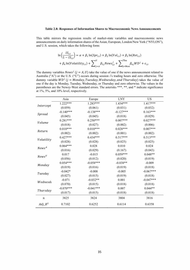
35

Table 2.8: Responses of Information Shares to Macroeconomic News Announcements

This table mirrors the regression results of market-state variables and macroeconomic news

announcements on daily information shares of the Asian, European, London/New York (“NYLON”),

and U.S. session, which takes the following form:


1 − 𝐼𝑆𝑖.𝑡) = 𝛼 + 𝛽1 ln(𝑆𝑝𝑟𝑖.𝑡) + 𝛽2 ln(𝑉𝑜𝑙𝑖.𝑡) + 𝛽3 ln(𝑅𝑒𝑡𝑖.𝑡)

+ 𝛽4 ln(𝑉𝑜𝑙𝑎𝑡𝑖𝑙𝑖𝑡𝑦𝑖.𝑡) + ∑ 𝛽5𝑗𝑁𝑒𝑤𝑠𝑖,𝑡𝑗

𝑈

𝑗=𝐴+ ∑ 𝛽6𝑗𝑊𝐷𝑗

Thu

j=Mon+ 𝜖𝑖,𝑡

The dummy variables 𝑁𝑒𝑤𝑠𝑗 (𝑗 = 𝐴, 𝑈) take the value of one if the news announcement related to

Australia (“A”) or the U.S. (“U”) occurs during session i’s trading hours and zero otherwise. The

dummy variable 𝑊𝐷𝑗 (𝑗 = 𝑀𝑜𝑛𝑑𝑎𝑦, 𝑇𝑢𝑒𝑠𝑑𝑎𝑦, 𝑊𝑒𝑑𝑛𝑒𝑠𝑑𝑎𝑦, 𝑎𝑛𝑑 𝑇ℎ𝑢𝑟𝑠𝑑𝑎𝑦) takes the value of

one if the day is Monday, Tuesday, Wednesday, or Thursday and zero otherwise. The values in the

parentheses are the Newey-West standard errors. The asterisks ***, **, and * indicate significance

at 1%, 5%, and 10% level, respectively.

Asia Europe LNY US

𝐼𝑛𝑡𝑒𝑟𝑐𝑒𝑝𝑡 1.222***

(0.059)

1.283***

(0.061)

1.434***

(0.031)

1.417***

(0.032)

𝑆𝑝𝑟𝑒𝑎𝑑 -0.140***

(0.045)

-0.138***

(0.045)

-0.127***

(0.018)

0.163***

(0.029)


(0.018)

0.250***

(0.027)

0.007***

(0.002)

0.027***

(0.006)


(0.002)

0.010***

(0.002)

0.028***

(0.001)

0.007***

(0.002)


(0.028)

0.434***

(0.028)

0.517***

(0.025)

0.513***

(0.025)

𝑁𝑒𝑤𝑠𝐴 0.064***

(0.016)

0.028

(0.029)

0.010

(0.167)

0.024

(0.043)

𝑁𝑒𝑤𝑠𝑈 0.017

(0.056)

-0.015

(0.012)

0.059***

(0.020)

0.048**

(0.019)

𝑀𝑜𝑛𝑑𝑎𝑦 0.054***

(0.019)

-0.058***

(0.016)

-0.038**

(0.019)

-0.009

(0.018)

𝑇𝑢𝑒eday -0.042*

(0.027)

-0.008

(0.015)

-0.005

(0.019)

-0.067***

(0.018)

𝑊𝑒𝑑𝑛𝑒𝑠𝑑𝑎𝑦 -0.071

(0.070)

-0.032**

(0.015)

0.001

(0.018)

-0.047***

(0.018)

𝑇ℎ𝑢𝑟𝑠𝑑𝑎𝑦 -0.070***

(0.017)

-0.041***

(0.015)

0.007

(0.018)

0.044**

(0.018)

𝑛 3825 3824 3804 3816

𝐴𝑑𝑗_𝑅2 0.7102 0.6252 0.6114 0.6358

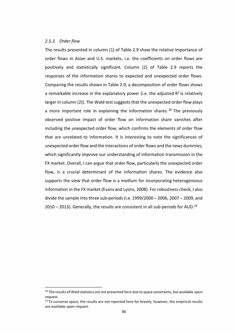
36

2.5.3. Order flow

The results presented in column (1) of Table 2.9 show the relative importance of

order flows in Asian and U.S. markets, i.e. the coefficients on order flows are

positively and statistically significant. Column (2) of Table 2.9 reports the

responses of the information shares to expected and unexpected order flows.

Comparing the results shown in Table 2.9, a decomposition of order flows shows

a remarkable increase in the explanatory power (i.e. the adjusted R2 is relatively

larger in column (2)). The Wald test suggests that the unexpected order flow plays

a more important role in explaining the information shares. 18 The previously

observed positive impact of order flow on information share vanishes after

including the unexpected order flow, which confirms the elements of order flow

that are unrelated to information. It is interesting to note the significances of

unexpected order flow and the interactions of order flows and the news dummies,

which significantly improve our understanding of information transmission in the

FX market. Overall, I can argue that order flow, particularly the unexpected order

flow, is a crucial determinant of the information shares. The evidence also

supports the view that order flow is a medium for incorporating heterogeneous

information in the FX market (Evans and Lyons, 2008). For robustness check, I also

divide the sample into three sub-periods (i.e. 1999/2000 – 2006, 2007 – 2009, and

2010 – 2013). Generally, the results are consistent in all sub-periods for AUD.19

18 The results of Wald statistics are not presented here due to space constraints, but available upon request. 19 To conserve space, the results are not reported here for brevity, however, the empirical results are available upon request.

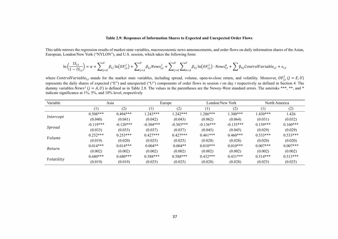
37

Table 2.9: Responses of Information Shares to Expected and Unexpected Order Flows

This table mirrors the regression results of market-state variables, macroeconomic news announcements, and order flows on daily information shares of the Asian,

European, London/New York (“NYLON”), and U.S. session, which takes the following form:


1 − 𝐼𝑆𝑖.𝑡) = 𝛼 + ∑ 𝛽1𝑗 ln(𝑂𝐹𝑖,𝑡

𝑗)

𝑈

𝑗=𝐸+ ∑ 𝛽2𝑗𝑁𝑒𝑤𝑠𝑖,𝑡

𝑗𝑈

𝑗=𝐴+ ∑ ∑ 𝛽3𝑗 ln(𝑂𝐹𝑖,𝑡


𝑘𝑈

𝑘=𝐴

𝑈

𝑗=𝐸+ ∑ β4𝑗𝐶𝑜𝑛𝑡𝑟𝑜𝑙𝑉𝑎𝑟𝑖𝑎𝑏𝑙𝑒𝑖,𝑡 + 𝜖𝑖,𝑡

where 𝐶𝑜𝑛𝑡𝑟𝑜𝑙𝑉𝑎𝑟𝑖𝑎𝑏𝑙𝑒𝑖,𝑡 stands for the market state variables, including spread, volume, open-to-close return, and volatility. Moreover, 𝑂𝐹𝑖,𝑡𝐽 (𝐽 = 𝐸, 𝑈)

represents the daily shares of expected (“E”) and unexpected (“U”) components of order flows in session i on day t respectively as defined in Section 4. The

dummy variables 𝑁𝑒𝑤𝑠𝑗 (𝑗 = 𝐴, 𝑈) is defined as in Table 2.8. The values in the parentheses are the Newey-West standard errors. The asterisks ***, **, and *

indicate significance at 1%, 5%, and 10% level, respectively


(1) (2) (1) (2) (1) (2) (1) (2)


(0.040)

0.494***

(0.041)

1.243***

(0.042)

1.242***

(0.043)

1.286***

(0.062)

1.300***

(0.064)

1.430***

(0.031)

1.426

(0.032)

𝑆𝑝𝑟𝑒𝑎𝑑 -0.119***

(0.033)

-0.120***

(0.033)

-0.304***

(0.037)

-0.303***

(0.037)

-0.136***

(0.045)

-0.135***

(0.045)

0.159***

(0.029)

0.160***

(0.029)


(0.019)

0.253***

(0.020)

0.427***

(0.025)

0.427***

(0.025)

0.461***

(0.028)

0.460***

(0.028)

0.533***

(0.020)

0.533***

(0.020)


(0.002)

0.014***

(0.002)

0.004**

(0.002)

0.004**

(0.002)

0.010***

(0.002)

0.010***

(0.002)

0.007***

(0.002)

0.007***

(0.002)


(0.019)

0.680***

(0.019)

0.588***

(0.025)

0.588***

(0.025)

0.432***

(0.028)

0.431***

(0.028)

0.514***

(0.025)

0.513***

(0.025)

38

Table 2.9 (Continued)


(1) (2) (1) (2) (1) (2) (1) (2)

𝑁𝑒𝑤𝑠𝐴 0.056***

(0.011)

0.079***

(0.018)

0.062*

(0.043)

-0.050

(0.034)

-0.090

(0.097)

0.132

(0.193)

0.020*

(0.012)

0.028**

(0.011)

𝑁𝑒𝑤𝑠𝑈 0.070*

(0.040)

-0.061

(0.070)

-0.016

(0.010)

-0.014

(0.014)

0.039*

(0.022)

0.069**

(0.029)

0.039

(0.025)

0.046***

(0.015)

𝑂𝐹 0.014***

(0.005)

0.005

(0.004)

0.004

(0.005)

0.010**

(0.004)

𝑂𝐹𝐸 0.005

(0.007)

0.004

(0.007)

0.007

(0.008)

0.011*

(0.006)

𝑂𝐹𝑈 0.015**

(0.006)

0.008*

(0.005)

0.037***

(0.007)

0.013**

(0.005)

𝑂𝐹𝐸 ∗ 𝑁𝑒𝑤𝑠𝐴 0.010*

(0.006)

-0.007

(0.018)

0.072

(0.088)

-0.011

(0.021)

𝑂𝐹𝐸 ∗ 𝑁𝑒𝑤𝑠𝑈 0.039

(0.029)

0.001

(0.008)

-0.013

(0.010)

0.017*

(0.009)

𝑂𝐹𝑈 ∗ 𝑁𝑒𝑤𝑠𝐴 0.008***

(0.001)

0.005

(0.019)

0.025

(0.085)

0.004

(0.022)

𝑂𝐹𝑈 ∗ 𝑁𝑒𝑤𝑠𝑈 0.033

(0.029)

0.002

(0.008)

0.011*

(0.006)

0.009**

(0.005)

𝑛 3819 3819 3818 3818 3798 3798 3809 3809

𝐴𝑑𝑗𝑢𝑠𝑡𝑒𝑑 𝑅2 0.8109 0.8310 0.7250 0.7353 0.7121 0.7520 0.7352 0.7854

39

2.5.4. Cross-market information flow and dynamic structure

The local- and cross-market information spillover are examined, and the results

are reported in Table 2.10. Reassuringly, I find that the main results in Table 2.9

remain intact. Namely, the conclusion regarding the importance of market state

variables remains unchanged, besides, the unexpected order flow and its

interaction with the news arrivals are most helpful in explaining the information

share of each trading session. As shown in Table 2.10, the coefficients of local-

market spillover effects as highlighted suggest the presence of first-order

autocorrelation of the dependent variable. The cross-market effects are

represented by the coefficients of lagged IS of other trading sessions, which

suggests negative relationships between information shares of each session and a

high information share of one trading session is associated with decreased share

of other trading sessions. Similar results have been reported in Gau and Wu (2017).

After controlling for the local- and cross-market information spillover effects, the

coefficients of unexpected order flow and its interaction with news arrivals remain

positive and significant.

In Table 2.10, I also include the dummy variable GFC in the regression which takes

the value of 1 during the period of Global Financial Crisis (2008:09–2009:11), and

0 otherwise. Interestingly, the empirical results suggest that the US played more

important role during the GFC period, while Europe markets became less

important. Therefore, with larger information share, the U.S. became more

efficient at incorporating the information into the fundamental prices related to

the exchange rates during the GFC period. The results here are generally

consistent with the findings in Section 2.2. For example, the US market contributes

more to the price discovery during the GFC period (i.e., 2008 - 2009) as shown in

Table 2.3 of the yearly average information shares.

40

Table 2.10: Responses of Information Shares to Order Flows and Macroeconomic News with Information Spillover

This table mirrors the regression results of own- and cross-market information spillover, market-state variables and macroeconomic news on daily information

shares of the Asian, European, London/New York (“NYLON”), and U.S. market, which takes the following form:

ln (𝐼𝑆𝑖,𝑡

1 − 𝐼𝑆𝑖,𝑡) = 𝛼 + ∑ 𝛽1,𝑗 ln (


1 − 𝐼𝑆𝑗,𝑡−1)

𝑈

𝑗=𝐴+ ∑ 𝛽2𝑗 ln(𝑂𝐹𝑖,𝑡

𝑗)

𝑈

𝑗=𝐸+ ∑ 𝛽3𝑗𝑁𝑒𝑤𝑠𝑖,𝑡

𝑗𝑈

𝑗=𝐴+ ∑ ∑ 𝛽4𝑗 ln(𝑂𝐹𝑖,𝑡


𝑘𝑈

𝑘=𝐴

𝑈

𝑗=𝐸+ ∑ 𝛽𝑖𝐶𝑜𝑛𝑡𝑟𝑜𝑙𝑉𝑎𝑟𝑖𝑎𝑏𝑙𝑒𝑖,𝑡 + 𝛽𝐺𝐹𝐶𝐺𝐹𝐶

+ ϵi,t

where 𝐶𝑜𝑛𝑡𝑟𝑜𝑙𝑉𝑎𝑟𝑖𝑎𝑏𝑙𝑒 includes all the market state variables as defined in Table 2.7, such as spread, volume, open-to-close return, and volatility. GFC is a

dummy variable for the 2008 Global Financial Crisis which equals 1 for the key financial crisis months of 2008:09–2009:11, and otherwise zero. In this equation,

the information spillover is typically represented by the coefficients of one-day lagged 𝐼𝑆𝑗,𝑡−1 (𝑗 = 𝐴, 𝐸, 𝐿, 𝑎𝑛𝑑 𝑈). Namely, the own-market spillover effect is

represented here by the coefficient of its own lagged IS 𝛽1,𝑗 (𝑗 = 𝑖), while the coefficients 𝛽1,𝑗 (𝑗 ≠ 𝑖) , which measure the short-run information spillover from

session j to session i, serve as a proxy for cross-market effects. Note that the subscript t-1 represents the session immediately before session i, which may be on

the same day as session i. For example, when i = Asia, 𝐼𝑆𝑖,𝑡−1 (𝑖 = 𝐴, 𝐸, 𝐿, 𝑎𝑛𝑑 𝑈) are IS from the previous day t – 1. However, when i = U.S., which is the last

trading session on day t, 𝐼𝑆𝑖,𝑡−1 (𝑖 = 𝐴, 𝐸, 𝐿) are from the same day t as US market with only the lagged U.S. information share 𝐼𝑆𝑖,𝑡−1 (𝑖 = 𝑈) from the previous

day. The values in the parentheses are the t-statistics based on Newey-West standard errors. The values highlighted in the table represents for the own-market

spillover effects. The asterisks ***, **, and * indicate significance at 1%, 5%, and 10% level, respectively


𝐼𝑆_𝐴𝑠𝑖𝑎_𝑙𝑎𝑔 0.0408***

(2.31)

-0.2216***

(-14.93)

-0.3381***

(-15.61)

-0.8465***

(-13.60)

𝐼𝑆_𝐸𝑢𝑟𝑜_lag -0.0218

(-0.92)

0.0171*

(1.64)

-0.0548*

(-2.22)

-0.4386***

(-19.89)

𝐼𝑆_𝐿𝑁𝑌_lag -0.0160*

(-1.64)

0.0005

(0.06)

0.0181**

(2.09)

-.5557***

(-16.04)

𝐼𝑆_𝑈𝑆_lag -0.1247***

(-3.12)

-0.0273***

(-2.78)

0.0013

(0.13)

0.0117*

(1.61)

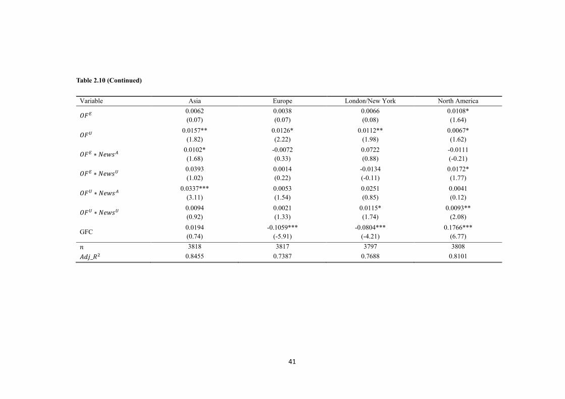
41



𝑂𝐹𝐸 0.0062

(0.07)

0.0038

(0.07)

0.0066

(0.08)

0.0108*

(1.64)

𝑂𝐹𝑈 0.0157**

(1.82)

0.0126*

(2.22)

0.0112**

(1.98)

0.0067*

(1.62)

𝑂𝐹𝐸 ∗ 𝑁𝑒𝑤𝑠𝐴 0.0102*

(1.68)

-0.0072

(0.33)

0.0722

(0.88)

-0.0111

(-0.21)


(1.02)

0.0014

(0.22)

-0.0134

(-0.11)

0.0172*

(1.77)

𝑂𝐹𝑈 ∗ 𝑁𝑒𝑤𝑠𝐴 0.0337***

(3.11)

0.0053

(1.54)

0.0251

(0.85)

0.0041

(0.12)


(0.92)

0.0021

(1.33)

0.0115*

(1.74)

0.0093**

(2.08)

GFC 0.0194

(0.74)

-0.1059***

(-5.91)

-0.0804***

(-4.21)

0.1766***

(6.77)

𝑛 3818 3817 3797 3808

𝐴𝑑𝑗_𝑅2 0.8455 0.7387 0.7688 0.8101

42

2.5.5. Market development and financial integration indicators

The estimation results of long-run determinants are reported in Table 2.11.20 First

of all, the pricing efficiency, which can be seen as an indicator of FX market

development, has a positive and significant impact on price discovery. Second,

with more active quoting banks in Asian trading hours, particularly with the

increasing participation of foreign banks headquartered overseas, the information

share of Asia increases substantially. These findings suggest that, with an

increasing degree of market integration and consolidation (i.e. with more active

dealing banks in the Asian market), Asia is playing an increasingly important role

in the price discovery of global FX trading. Besides, the number of quoting banks

has a significantly and positively effect on information shares for all markets.

However, the percentage of foreign banks is not useful in explaining the

information shares except for that in the Asian market, which is probably due to

the fact that a larger proportion of FX trading has been conducted between

counterparties located in the same place, but their headquarters could be

elsewhere (BIS, 2013).

Furthermore, I consider the impact of market concentration on price discovery.

There is a long-standing debate about the influences of market concentration. For

example, on the one hand, the market concentration enables the top-tier banks

to process greater order flow and internalize customer order flow, which helps

them aggregate the dispersed information among the customers and contribute

more to the price discovery (Evans, 2002; Evans and Lyons, 2002a; Rime and

Schrimpf, 2013). On the other hand, the market concentration may cause erratic

swings amid liquidity drought, especially during times of market stress (Yin, 2005;

Hendershott and Jones, 2005). The empirical results suggest that the increasing

market concentration does not have a consistent effect on the price discovery,

which confirms the ambiguous effect of market concentration as documented in

previous studies.

20 Following the suggestions of the thesis examiner, I report the summary statistics of long-run determinants in Appendix C.

43

Finally, considering the importance of financial market infrastructure in facilitating

the price discovery process, I include the GDP-weighted average Chinn-Ito Index

in the regression to proxy for the degree of capital market openness and financial

liberalization. The empirical results presented in Table 2.11 confirm that the

overall Chinn-Ito Index have a positive effect on the information shares in all

sessions. This effect is particularly high in the Asian market. In overall terms, a

higher degree of FX market development and financial integration is highly

desirable, particularly for Asian market.

The estimations of long-run determinants with lead-lag effects are shown in Table

2.12. The lagged term of IS has significantly positive effects on the monthly

information share of each trading session. Furthermore, to control for seasonality

as shown in Figure 2.2, I add the 12-month lagged IS in the regression. The results

suggest the presence of seasonality and re-confirm the conclusions about the

fundamental effects of the proxy variables for the degree of financial market

development and integration.

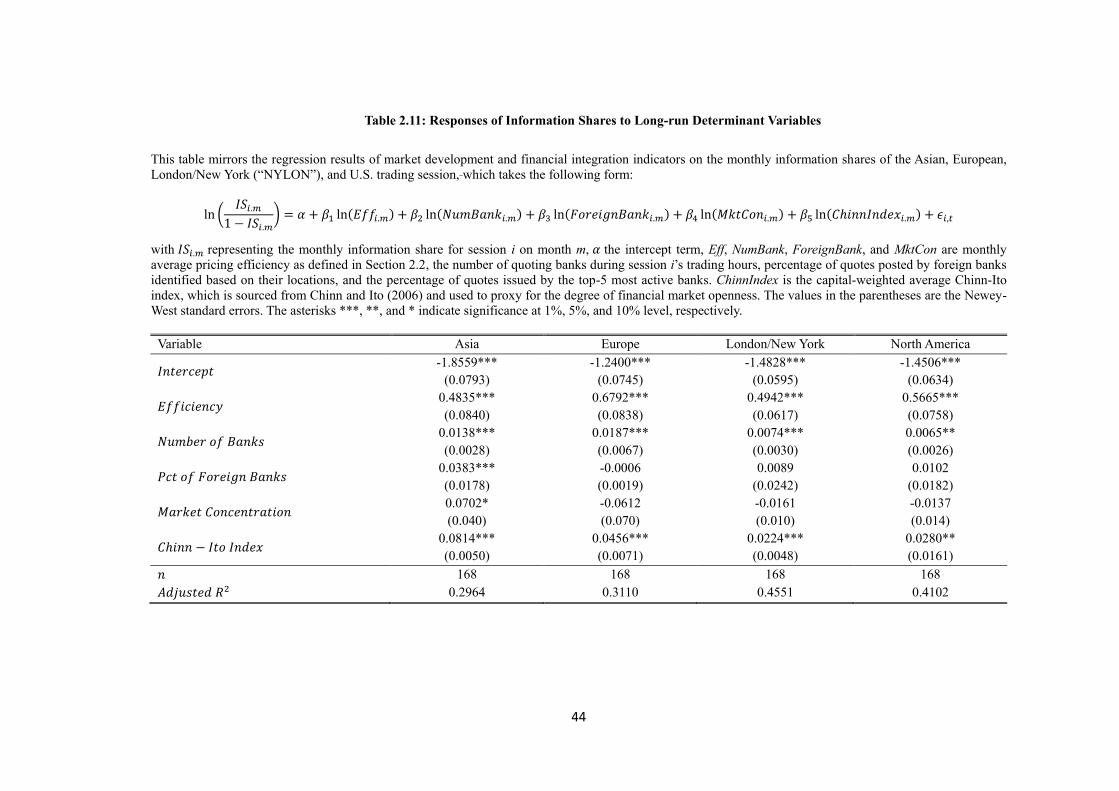
44

Table 2.11: Responses of Information Shares to Long-run Determinant Variables

This table mirrors the regression results of market development and financial integration indicators on the monthly information shares of the Asian, European,

London/New York (“NYLON”), and U.S. trading session, which takes the following form:

ln (𝐼𝑆𝑖.𝑚

1 − 𝐼𝑆𝑖.𝑚) = 𝛼 + 𝛽1 ln(𝐸𝑓𝑓𝑖.𝑚) + 𝛽2 ln(𝑁𝑢𝑚𝐵𝑎𝑛𝑘𝑖.𝑚) + 𝛽3 ln(𝐹𝑜𝑟𝑒𝑖𝑔𝑛𝐵𝑎𝑛𝑘𝑖.𝑚) + 𝛽4 ln(𝑀𝑘𝑡𝐶𝑜𝑛𝑖.𝑚) + 𝛽5 ln(𝐶ℎ𝑖𝑛𝑛𝐼𝑛𝑑𝑒𝑥𝑖.𝑚) + 𝜖𝑖,𝑡

with 𝐼𝑆𝑖.𝑚 representing the monthly information share for session i on month m, 𝛼 the intercept term, Eff, NumBank, ForeignBank, and MktCon are monthly

average pricing efficiency as defined in Section 2.2, the number of quoting banks during session i’s trading hours, percentage of quotes posted by foreign banks

identified based on their locations, and the percentage of quotes issued by the top-5 most active banks. ChinnIndex is the capital-weighted average Chinn-Ito

index, which is sourced from Chinn and Ito (2006) and used to proxy for the degree of financial market openness. The values in the parentheses are the Newey-

West standard errors. The asterisks ***, **, and * indicate significance at 1%, 5%, and 10% level, respectively.


𝐼𝑛𝑡𝑒𝑟𝑐𝑒𝑝𝑡 -1.8559***

(0.0793)

-1.2400***

(0.0745)

-1.4828***

(0.0595)

-1.4506***

(0.0634)

𝐸𝑓𝑓𝑖𝑐𝑖𝑒𝑛𝑐𝑦 0.4835***

(0.0840)

0.6792***

(0.0838)

0.4942***

(0.0617)

0.5665***

(0.0758)

𝑁𝑢𝑚𝑏𝑒𝑟 𝑜𝑓 𝐵𝑎𝑛𝑘𝑠 0.0138***

(0.0028)

0.0187***

(0.0067)

0.0074***

(0.0030)

0.0065**

(0.0026)

𝑃𝑐𝑡 𝑜𝑓 𝐹𝑜𝑟𝑒𝑖𝑔𝑛 𝐵𝑎𝑛𝑘𝑠 0.0383***

(0.0178)

-0.0006

(0.0019)

0.0089

(0.0242)

0.0102

(0.0182)

𝑀𝑎𝑟𝑘𝑒𝑡 𝐶𝑜𝑛𝑐𝑒𝑛𝑡𝑟𝑎𝑡𝑖𝑜𝑛 0.0702*

(0.040)

-0.0612

(0.070)

-0.0161

(0.010)

-0.0137

(0.014)

𝐶ℎ𝑖𝑛𝑛 − 𝐼𝑡𝑜 𝐼𝑛𝑑𝑒𝑥 0.0814***

(0.0050)

0.0456***

(0.0071)

0.0224***

(0.0048)

0.0280**

(0.0161)

𝑛 168 168 168 168

𝐴𝑑𝑗𝑢𝑠𝑡𝑒𝑑 𝑅2 0.2964 0.3110 0.4551 0.4102

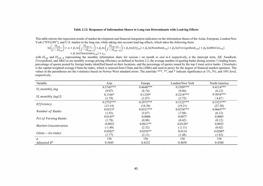
45

Table 2.12: Responses of Information Shares to Long-run Determinants with Lead-lag Effects

This table mirrors the regression results of market development and financial integration indicators on the information shares of the Asian, European, London/New

York (“NYLON”), and U.S. market in the long run, while taking into account lead-lag effects, which takes the following form:

ln (𝐼𝑆𝑖,𝑚

1 − 𝐼𝑆𝑖,𝑚) = 𝛼 + 𝛽1 ln (


1 − 𝐼𝑆𝑖,𝑚−1) + 𝛽2 ln (


1 − 𝐼𝑆𝑖,𝑚−12) + 𝛽3 ln(𝐸𝑓𝑓𝑖.𝑚) + 𝛽4 ln(𝑁𝑢𝑚𝐵𝑎𝑛𝑘𝑖.𝑚) + 𝛽5 ln(𝐹𝑜𝑟𝑒𝑖𝑔𝑛𝐵𝑎𝑛𝑘𝑖.𝑚) + 𝛽6 ln(𝑀𝑘𝑡𝐶𝑜𝑛𝑖.𝑚)

+ 𝛽7 ln(𝐶ℎ𝑖𝑛𝑛𝐼𝑛𝑑𝑒𝑥𝑖.𝑚) + 𝜖𝑖,𝑡

with 𝐼𝑆𝑖.𝑚 and 𝐼𝑆𝑖.𝑚−𝑘 representing the monthly information share for session i on month m and m-k respectively, 𝛼 the intercept term, Eff, NumBank,

ForeignBank, and MktCon are monthly average pricing efficiency as defined in Section 2.2, the average number of quoting banks during session i’s trading hours,

percentage of quotes posted by foreign banks identified based on their locations, and the percentage of quotes issued by the top-5 most active banks. ChinnIndex

is the capital-weighted average Chinn-Ito index, which is sourced from Chinn and Ito (2006) and used to proxy for the degree of financial market openness. The

values in the parentheses are the t-statistics based on Newey-West standard errors. The asterisks ***, **, and * indicate significance at 1%, 5%, and 10% level,

respectively.


𝐼𝑆_𝑚𝑜𝑛𝑡ℎ𝑙𝑦_𝑙𝑎𝑔 0.5745***

(9.07)

0.4648***

(6.74)

0.5589***

(9.86)

0.4114***

(6.12)

𝐼𝑆_𝑚𝑜𝑛𝑡ℎ𝑙𝑦_𝑙𝑎𝑔12 0.1166*

(1.79)

0.1230*

(1.87)

0.2218***

(3.75)

0.3018***

（4.47）

𝐸𝑓𝑓𝑖𝑐𝑖𝑒𝑛𝑐𝑦 0.2752***

(13.14)

0.2973***

(18.38)

0.3122***

(19.21)

0.3321***

(27.58)

𝑁𝑢𝑚𝑏𝑒𝑟 𝑜𝑓 𝐵𝑎𝑛𝑘𝑠 0.0233*

(1.83)

0.0321***

(5.67)

0.0754***

(7.88)

0.0665***

(6.12)

𝑃𝑐𝑡 𝑜𝑓 𝐹𝑜𝑟𝑒𝑖𝑛𝑔 𝐵𝑎𝑛𝑘𝑠 0.0145*

(1.78)

-0.0006

(0.88)

0.0077

(0.42)

0.0003

(0.12)

𝑀𝑎𝑟𝑘𝑒𝑡 𝐶𝑜𝑛𝑐𝑒𝑛𝑡𝑟𝑎𝑡𝑖𝑜𝑛 -0.0022

(-1.40)

0.0611**

(2.32)

-0.0126*

(-2.11)

0.0032

(0.42)

𝐶ℎ𝑖𝑛𝑛 − 𝐼𝑡𝑜 𝐼𝑛𝑑𝑒𝑥 0.0202*

(1.77)

0.0356**

(2.11)

0.0114

(1.48)

0.0280*

(1.65)

𝑛 156 156 156 156

𝐴𝑑𝑗𝑢𝑠𝑡𝑒𝑑 𝑅2 0.3645 0.4232 0.4858 0.4380

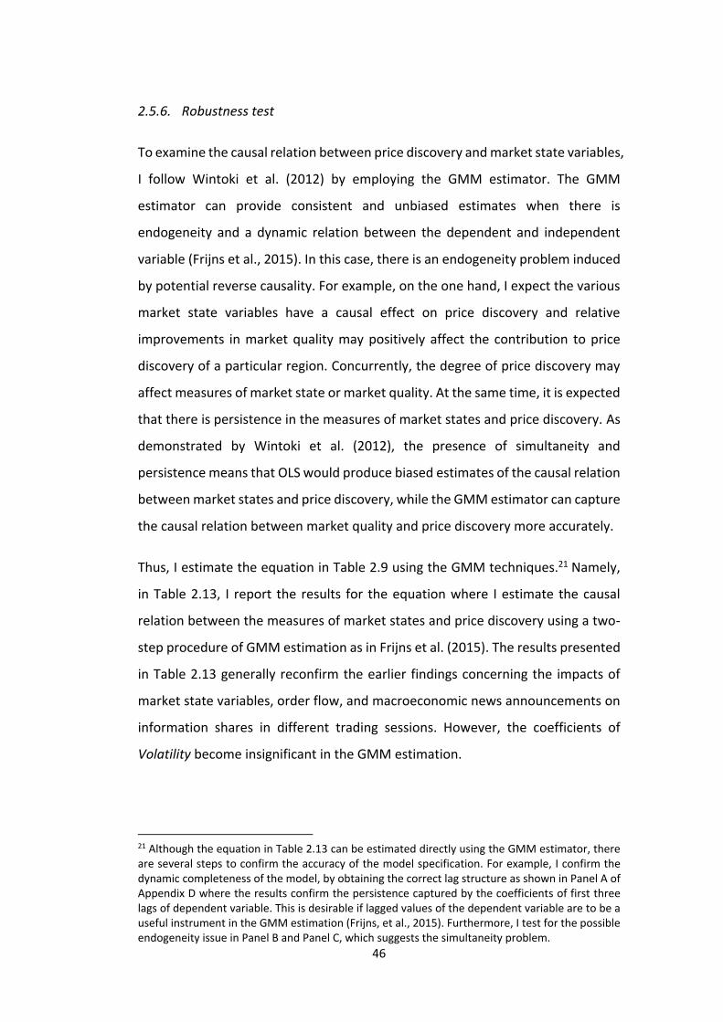
46

2.5.6. Robustness test

To examine the causal relation between price discovery and market state variables,

I follow Wintoki et al. (2012) by employing the GMM estimator. The GMM

estimator can provide consistent and unbiased estimates when there is

endogeneity and a dynamic relation between the dependent and independent

variable (Frijns et al., 2015). In this case, there is an endogeneity problem induced

by potential reverse causality. For example, on the one hand, I expect the various

market state variables have a causal effect on price discovery and relative

improvements in market quality may positively affect the contribution to price

discovery of a particular region. Concurrently, the degree of price discovery may

affect measures of market state or market quality. At the same time, it is expected

that there is persistence in the measures of market states and price discovery. As

demonstrated by Wintoki et al. (2012), the presence of simultaneity and

persistence means that OLS would produce biased estimates of the causal relation

between market states and price discovery, while the GMM estimator can capture

the causal relation between market quality and price discovery more accurately.

Thus, I estimate the equation in Table 2.9 using the GMM techniques.21 Namely,

in Table 2.13, I report the results for the equation where I estimate the causal

relation between the measures of market states and price discovery using a two-

step procedure of GMM estimation as in Frijns et al. (2015). The results presented

in Table 2.13 generally reconfirm the earlier findings concerning the impacts of

market state variables, order flow, and macroeconomic news announcements on

information shares in different trading sessions. However, the coefficients of

Volatility become insignificant in the GMM estimation.

21 Although the equation in Table 2.13 can be estimated directly using the GMM estimator, there are several steps to confirm the accuracy of the model specification. For example, I confirm the dynamic completeness of the model, by obtaining the correct lag structure as shown in Panel A of Appendix D where the results confirm the persistence captured by the coefficients of first three lags of dependent variable. This is desirable if lagged values of the dependent variable are to be a useful instrument in the GMM estimation (Frijns, et al., 2015). Furthermore, I test for the possible endogeneity issue in Panel B and Panel C, which suggests the simultaneity problem.

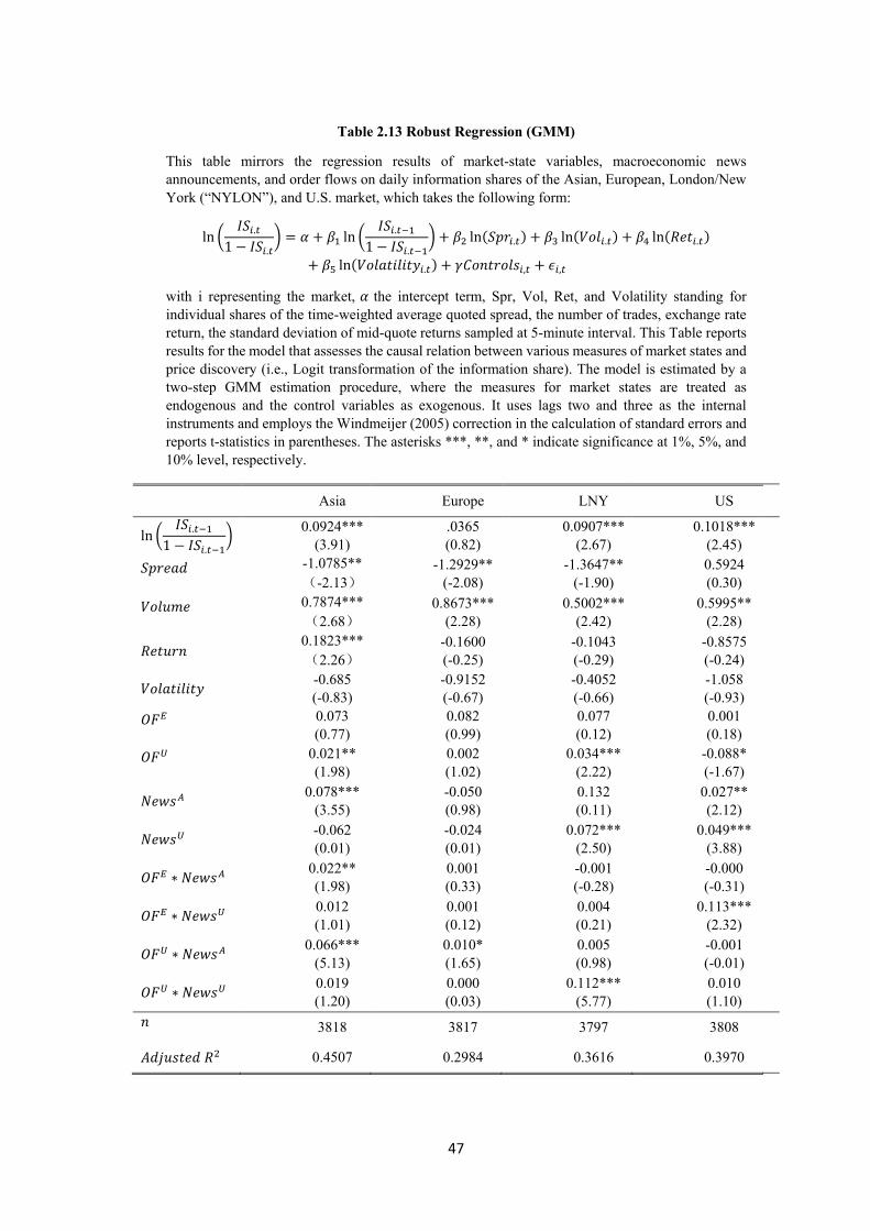
47

Table 2.13 Robust Regression (GMM)

This table mirrors the regression results of market-state variables, macroeconomic news

announcements, and order flows on daily information shares of the Asian, European, London/New

York (“NYLON”), and U.S. market, which takes the following form:


1 − 𝐼𝑆𝑖.𝑡) = 𝛼 + 𝛽1 ln (

𝐼𝑆𝑖.𝑡−1

1 − 𝐼𝑆𝑖.𝑡−1) + 𝛽2 ln(𝑆𝑝𝑟𝑖.𝑡) + 𝛽3 ln(𝑉𝑜𝑙𝑖.𝑡) + 𝛽4 ln(𝑅𝑒𝑡𝑖.𝑡)

+ 𝛽5 ln(𝑉𝑜𝑙𝑎𝑡𝑖𝑙𝑖𝑡𝑦𝑖.𝑡) + 𝛾𝐶𝑜𝑛𝑡𝑟𝑜𝑙𝑠𝑖,𝑡 + 𝜖𝑖,𝑡

with i representing the market, 𝛼 the intercept term, Spr, Vol, Ret, and Volatility standing for

individual shares of the time-weighted average quoted spread, the number of trades, exchange rate

return, the standard deviation of mid-quote returns sampled at 5-minute interval. This Table reports

results for the model that assesses the causal relation between various measures of market states and

price discovery (i.e., Logit transformation of the information share). The model is estimated by a

two-step GMM estimation procedure, where the measures for market states are treated as

endogenous and the control variables as exogenous. It uses lags two and three as the internal

instruments and employs the Windmeijer (2005) correction in the calculation of standard errors and

reports t-statistics in parentheses. The asterisks ***, **, and * indicate significance at 1%, 5%, and

10% level, respectively.

Asia Europe LNY US

ln (𝐼𝑆𝑖.𝑡−1

1 − 𝐼𝑆𝑖.𝑡−1)

0.0924***

(3.91)

.0365

(0.82)

0.0907***

(2.67)

0.1018***

(2.45)

𝑆𝑝𝑟𝑒𝑎𝑑 -1.0785**

（-2.13）

-1.2929**

(-2.08)

-1.3647**

(-1.90)

0.5924

(0.30)

𝑉𝑜𝑙𝑢𝑚𝑒 0.7874***

（2.68）

0.8673***

(2.28)

0.5002***

(2.42)

0.5995**

(2.28)

𝑅𝑒𝑡𝑢𝑟𝑛 0.1823***

（2.26）

-0.1600

(-0.25)

-0.1043

(-0.29)

-0.8575

(-0.24)

𝑉𝑜𝑙𝑎𝑡𝑖𝑙𝑖𝑡𝑦 -0.685

(-0.83)

-0.9152

(-0.67)

-0.4052

(-0.66)

-1.058

(-0.93)

𝑂𝐹𝐸 0.073

(0.77)

0.082

(0.99)

0.077

(0.12)

0.001

(0.18)

𝑂𝐹𝑈 0.021**

(1.98)

0.002

(1.02)

0.034***

(2.22)

-0.088*

(-1.67)

𝑁𝑒𝑤𝑠𝐴 0.078***

(3.55)

-0.050

(0.98)

0.132

(0.11)

0.027**

(2.12)

𝑁𝑒𝑤𝑠𝑈 -0.062

(0.01)

-0.024

(0.01)

0.072***

(2.50)

0.049***

(3.88)

𝑂𝐹𝐸 ∗ 𝑁𝑒𝑤𝑠𝐴 0.022**

(1.98)

0.001

(0.33)

-0.001

(-0.28)

-0.000

(-0.31)


(1.01)

0.001

(0.12)

0.004

(0.21)

0.113***

(2.32)

𝑂𝐹𝑈 ∗ 𝑁𝑒𝑤𝑠𝐴 0.066***

(5.13)

0.010*

(1.65)

0.005

(0.98)

-0.001

(-0.01)


(1.20)

0.000

(0.03)

0.112***

(5.77)

0.010

(1.10)

𝑛 3818 3817 3797 3808

𝐴𝑑𝑗𝑢𝑠𝑡𝑒𝑑 𝑅2 0.4507 0.2984 0.3616 0.3970

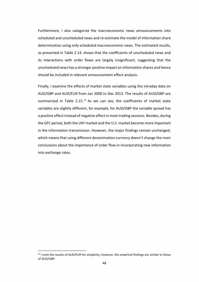
48

Furthermore, I also categorize the macroeconomic news announcements into

scheduled and unscheduled news and re-estimate the model of information share

determination using only scheduled macroeconomic news. The estimated results,

as presented in Table 2.14, shows that the coefficients of unscheduled news and

its interactions with order flows are largely insignificant, suggesting that the

unscheduled news has a stronger positive impact on information shares and hence

should be included in relevant announcement effect analysis.

Finally, I examine the effects of market state variables using the intraday data on

AUD/GBP and AUD/EUR from Jan 2000 to Dec 2013. The results of AUD/GBP are

summarized in Table 2.15. 22 As we can see, the coefficients of market state

variables are slightly different, for example, for AUD/GBP the variable spread has

a positive effect instead of negative effect in most trading sessions. Besides, during

the GFC period, both the LNY market and the U.S. market become more important

in the information transmission. However, the major findings remain unchanged,

which means that using different denomination currency doesn’t change the main

conclusions about the importance of order flow in incorporating new information

into exchange rates.

22 I omit the results of AUD/EUR for simplicity, however, the empirical findings are similar to those of AUD/GBP.

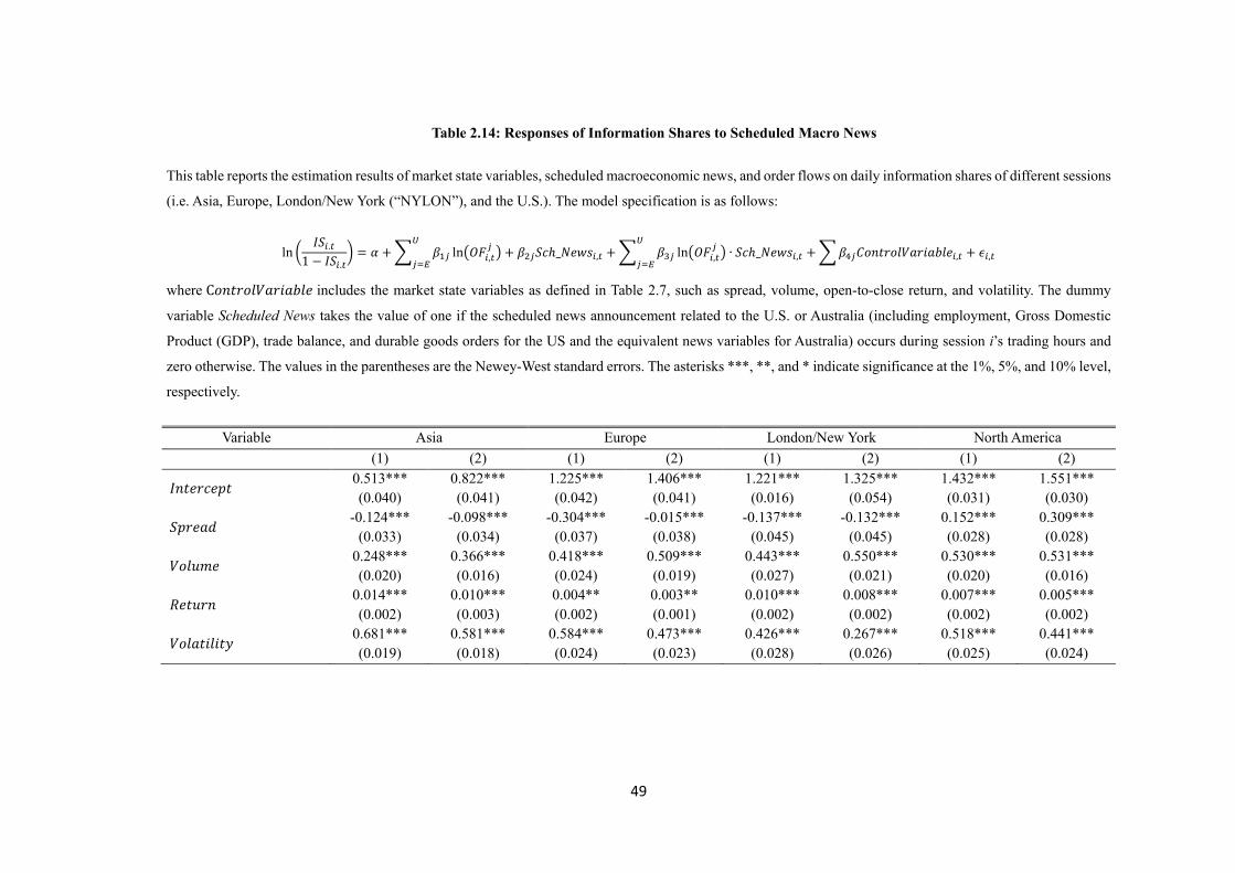
49

Table 2.14: Responses of Information Shares to Scheduled Macro News

This table reports the estimation results of market state variables, scheduled macroeconomic news, and order flows on daily information shares of different sessions

(i.e. Asia, Europe, London/New York (“NYLON”), and the U.S.). The model specification is as follows:


1 − 𝐼𝑆𝑖.𝑡) = 𝛼 + ∑ 𝛽1𝑗 ln(𝑂𝐹𝑖,𝑡

𝑗)

𝑈

𝑗=𝐸+ 𝛽2𝑗𝑆𝑐ℎ_𝑁𝑒𝑤𝑠𝑖,𝑡 + ∑ 𝛽3𝑗 ln(𝑂𝐹𝑖,𝑡

𝑗) ∙ 𝑆𝑐ℎ_𝑁𝑒𝑤𝑠𝑖,𝑡

𝑈

𝑗=𝐸+ ∑ 𝛽4𝑗𝐶𝑜𝑛𝑡𝑟𝑜𝑙𝑉𝑎𝑟𝑖𝑎𝑏𝑙𝑒𝑖,𝑡 + 𝜖𝑖,𝑡

where C𝑜𝑛𝑡𝑟𝑜𝑙𝑉𝑎𝑟𝑖𝑎𝑏𝑙𝑒 includes the market state variables as defined in Table 2.7, such as spread, volume, open-to-close return, and volatility. The dummy

variable Scheduled News takes the value of one if the scheduled news announcement related to the U.S. or Australia (including employment, Gross Domestic

Product (GDP), trade balance, and durable goods orders for the US and the equivalent news variables for Australia) occurs during session i’s trading hours and

zero otherwise. The values in the parentheses are the Newey-West standard errors. The asterisks ***, **, and * indicate significance at the 1%, 5%, and 10% level,

respectively.


(1) (2) (1) (2) (1) (2) (1) (2)


(0.040)

0.822***

(0.041)

1.225***

(0.042)

1.406***

(0.041)

1.221***

(0.016)

1.325***

(0.054)

1.432***

(0.031)

1.551***

(0.030)

𝑆𝑝𝑟𝑒𝑎𝑑 -0.124***

(0.033)

-0.098***

(0.034)

-0.304***

(0.037)

-0.015***

(0.038)

-0.137***

(0.045)

-0.132***

(0.045)

0.152***

(0.028)

0.309***

(0.028)


(0.020)

0.366***

(0.016)

0.418***

(0.024)

0.509***

(0.019)

0.443***

(0.027)

0.550***

(0.021)

0.530***

(0.020)

0.531***

(0.016)


(0.002)

0.010***

(0.003)

0.004**

(0.002)

0.003**

(0.001)

0.010***

(0.002)

0.008***

(0.002)

0.007***

(0.002)

0.005***

(0.002)


(0.019)

0.581***

(0.018)

0.584***

(0.024)

0.473***

(0.023)

0.426***

(0.028)

0.267***

(0.026)

0.518***

(0.025)

0.441***

(0.024)

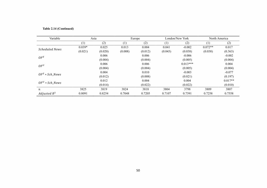
50



(1) (2) (1) (2) (1) (2) (1) (2)

𝑆𝑐ℎ𝑒𝑑𝑢𝑙𝑒𝑑 𝑁𝑒𝑤𝑠 0.039*

(0.021)

0.025

(0.020)

0.013

(0.008)

0.004

(0.012)

0.041

(0.043)

-0.002

(0.038)

0.072**

(0.038)

0.017

(0.363)

𝑂𝐹𝐸 0.006

(0.004)

0.006

(0.004)

-0.006

(0.005)

-0.002

(0.004)

𝑂𝐹𝑈 0.006

(0.004)

0.006

(0.004)

0.013***

(0.005)

0.004

(0.004)

𝑂𝐹𝐸 ∗ 𝑆𝑐ℎ_𝑁𝑒𝑤𝑠 0.004

(0.012)

0.010

(0.008)

-0.003

(0.021)

-0.077

(0.197)

𝑂𝐹𝑈 ∗ 𝑆𝑐ℎ_𝑁𝑒𝑤𝑠 0.012

(0.014)

0.004

(0.022)

0.004

(0.022)

0.017**

(0.010)

𝑛 3825 3819 3824 3818 3804 3798 3809 3807

𝐴𝑑𝑗𝑢𝑠𝑡𝑒𝑑 𝑅2 0.8091 0.8254 0.7048 0.7205 0.7107 0.7391 0.7258 0.7558

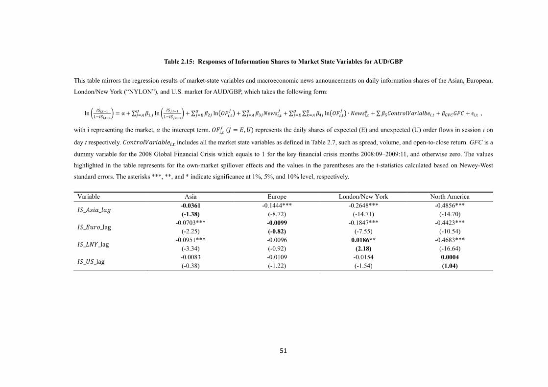
51

Table 2.15: Responses of Information Shares to Market State Variables for AUD/GBP

This table mirrors the regression results of market-state variables and macroeconomic news announcements on daily information shares of the Asian, European,

London/New York (“NYLON”), and U.S. market for AUD/GBP, which takes the following form:

ln (𝐼𝑆𝑖,𝑡−1

1−𝐼𝑆𝑖,𝑡−1) = α + ∑ 𝛽1,𝑗 ln (


1−𝐼𝑆𝑗,𝑡−1)𝑈

𝑗=𝐴 + ∑ 𝛽2𝑗 ln(𝑂𝐹𝑖,𝑡𝑗


𝑗𝑈𝑗=𝐴 + ∑ ∑ 𝛽4𝑗 ln(𝑂𝐹𝑖,𝑡


𝑘𝑈𝑘=𝐴

𝑈𝑗=𝐸 + ∑ 𝛽5𝐶𝑜𝑛𝑡𝑟𝑜𝑙𝑉𝑎𝑟𝑖𝑎𝑙𝑏𝑒𝑖,𝑡 + 𝛽𝐺𝐹𝐶𝐺𝐹𝐶 + ϵi,t ,

with i representing the market, 𝛼 the intercept term. 𝑂𝐹𝑖,𝑡𝐽 (𝐽 = 𝐸, 𝑈) represents the daily shares of expected (E) and unexpected (U) order flows in session i on

day t respectively. 𝐶𝑜𝑛𝑡𝑟𝑜𝑙𝑉𝑎𝑟𝑖𝑎𝑏𝑙𝑒𝑖,𝑡 includes all the market state variables as defined in Table 2.7, such as spread, volume, and open-to-close return. GFC is a

dummy variable for the 2008 Global Financial Crisis which equals to 1 for the key financial crisis months 2008:09–2009:11, and otherwise zero. The values

highlighted in the table represents for the own-market spillover effects and the values in the parentheses are the t-statistics calculated based on Newey-West

standard errors. The asterisks ***, **, and * indicate significance at 1%, 5%, and 10% level, respectively.


𝐼𝑆_𝐴𝑠𝑖𝑎_𝑙𝑎𝑔 -0.0361

(-1.38)

-0.1444***

(-8.72)

-0.2648***

(-14.71)

-0.4856***

(-14.70)

𝐼𝑆_𝐸𝑢𝑟𝑜_lag -0.0703***

(-2.25)

-0.0099

(-0.82)

-0.1847***

(-7.55)

-0.4423***

(-10.54)

𝐼𝑆_𝐿𝑁𝑌_lag -0.0951***

(-3.34)

-0.0096

(-0.92)

0.0186**

(2.18)

-0.4683***

(-16.64)

𝐼𝑆_𝑈𝑆_lag -0.0083

(-0.38)

-0.0109

(-1.22)

-0.0154

(-1.54)

0.0004

(1.04)

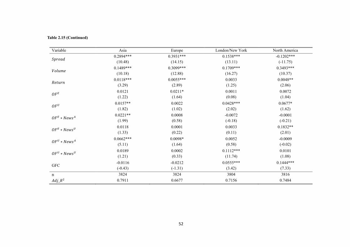
52



𝑆𝑝𝑟𝑒𝑎𝑑 0.2894***

(10.48)

0.3931***

(14.15)

0.1538***

(13.11)

-0.1202***

(-11.75)

𝑉𝑜𝑙𝑢𝑚𝑒 0.1489***

(10.18)

0.3099***

(12.88)

0.1709***

(16.27)

0.3493***

(10.37)

𝑅𝑒𝑡𝑢𝑟𝑛 0.0118***

(3.29)

0.0055***

(2.89)

0.0033

(1.25)

0.0048**

(2.06)

𝑂𝐹𝐸 0.0121

(1.22)

0.0211*

(1.64)

0.0011

(0.08)

0.0072

(1.04)

𝑂𝐹𝑈 0.0157**

(1.82)

0.0022

(1.02)

0.0428***

(2.02)

0.0677*

(1.62)

𝑂𝐹𝐸 ∗ 𝑁𝑒𝑤𝑠𝐴 0.0221**

(1.99)

0.0008

(0.58)

-0.0072

(-0.18)

-0.0001

(-0.21)


(1.33)

0.0001

(0.22)

0.0033

(0.11)

0.1832**

(2.01)

𝑂𝐹𝑈 ∗ 𝑁𝑒𝑤𝑠𝐴 0.0662***

(5.11)

0.0098*

(1.64)

0.0052

(0.58)

-0.0009

(-0.02)


(1.21)

0.0002

(0.33)

0.1112***

(11.74)

0.0101

(1.08)

GFC -0.0116

(-0.43)

-0.0212

(-1.31)

0.0555***

(3.42)

0.1444***

(7.33)

n 3824 3824 3804 3816

𝐴𝑑𝑗_𝑅2 0.7911 0.6677 0.7156 0.7484

53

2.6. Conclusions and policy implications

With rapid growth in emerging economies, such as China and India, the demand

for Australia’s natural resources has increased substantially. As a result, the role

of the Australian dollar (AUD) in the global financial markets has become more

important (McCauley, 2006). Using firm quotes and trading data from January

1999 to December 2013, this chapter estimates the global information distribution

of AUD trading in the Asian, European, and North American markets. Specifically,

using the price quotes of AUD against the US dollar over a relatively long period

(i.e. 15 years in total), I employ a non-parametric price discovery methodology, i.e.,

Two-scale Realized Variance (TSRV) ratio, to estimate the information shares of

global AUD trading. I find that the European market and U.S. market, particularly

the overlapping trading session of London and New York, dominate in price

discovery process in AUD market, but Asia is rapidly gaining information shares

even with its declining market share of daily transactions.

After estimating the information share, I focus on its short- and long-run

determinants in each market. Namely, I consider the effects of macroeconomic

news, order flow measures, market state variables while taking into account cross-

market effects and dynamic completeness of information shares in each trading

session. The empirical analysis shows that more favourable market states and

more unexpected order flows, particularly on macroeconomic announcement

days, make a significantly positive contribution to price discovery in all trading

sessions for AUD trading. Meanwhile, there are strong information spillover

effects in the FX market, and high information share of one trading session is

associated with increased information share in the future, while decreased

information share of other trading sessions. The empirical results also confirm

that a higher degree of market integration and international consolidation

contributes to price discovery in the long-run.

The distinguishing feature of this chapter is that I consider the impact of a broader

set of news announcements on information shares, which includes both scheduled

and unscheduled news announcements. Besides, I show that the decomposition

54

of order flows into an expectation-related and an innovation term can significantly

improve our understanding of the dealer behaviour responding to different types

of information arrival. This chapter also contribute to the literature on price

discovery by considering the long-run determinants of information shares.

Specifically, I attempt to explore the relationship between the price discovery,

market integration, and the development of financial markets. The empircal

results are generally consistent with Sassen (1999) who claims that the two most

important factors in transforming a city into a global financial centre are

international consolidation of financial activities and financial market

liberalization.

This study on price discovery in AUD market has some important policy

implications, especially for financial centres in the Asia-Pacific region. For example,

the empirical results suggest that the financial market openness and liberalization

have a strong impact on the long-run trends in price discovery. To better compete

with the leading financial centres in North America and Europe, the Asian financial

centres need to be more open to international investors and adopt global

principles of financial market regulations. Furthermore, the findings of inter- and

intra-regional information spillover effects suggest that price discovery is sticky

and persistent. Hence the improvement of price discovery in Asia can gain a

competitive edge over other regions in the long-run.

The research presented in this chapter can also be extended in several directions.

For example, how to accurately measure the information shares in the financial

markets is one question that is yet to be fully answered. Furthermore, additional

research is required to consider the generalizability of these results. This will

involve considering price discovery of other major currencies and emerging

currencies. Last but not least, the issue of how to identify volatility jumps

associated with macroeconomic news announcements deserves further study,

which will definitely improve the measure of information shares and extend our

understanding in economic intuition of price discovery in the foreign exchange

market.

55

Chapter 3: Meteor Showers and Heat Waves Effects in the Foreign

Exchange Market: Some New Evidence

3.1. Introduction

The development of estimators of volatility based on high-frequency information

has led to large improvements in measuring financial market volatility. The

investigation into volatility spillovers across geographical regions is an import topic,

which contributes to our knowledge about global financial interconnectedness.

The phenomenon of volatility spillover occurs when volatility in one market

triggers volatility in other markets. This effect can be particularly visible during

periods of turmoil which diminishes the benefits of international portfolio

diversification for investors. It is further amplified by the recent technological

advances, such as the rise of electronic trading and algorithm trading, which have

undoubtedly facilitated information flows. Besides, with the dominance of cross-

market effects in a wide range of financial markets, the financial instruments

become more temporally correlated across markets, which raises concerns from

regulators about global financial instability and contagion effects. The

international information transmission across markets through volatility have a

wide range of practical implications as well. For example, models incorporating

these features significantly improve volatility and these statistical improvements

can be translated into significant economic gains (Su, 2018).

In this paper, I mainly focus on the Foreign Exchange (FX) market which is the

largest financial market in the world, with a daily trading volume of about five

trillion U.S. dollars (Bank for International Settlements, 2013). Also, the FX market

is fairly opaque and decentralized because of its two-tier market structure when

compared to, for example, the major equity markets.23 Besides, unlike the equity

markets, the Foreign Exchange markets operate continuously from Asia to Europe,

then to America throughout the day. In sum, the size, sophistication, global

23 For a thorough introduction to the market structure and its evolution in the Foreign Exchange market, please refer to King, Osler, and Rime (2011).

56

perspective, and relative continuity of trading in the FX market make it an ideal

candidate for the study of volatility spillover and information propagation effects.

With the decentralised market structure, the question naturally arises: what drives

volatility spillovers in the FX market? This paper addresses several related

questions that arise in this market setting. First, I provide new evidence to the

debate on the patterns of volatility spillovers as documented in the previous study

and find evidence of both meteor shower (i.e. intra-regional volatility spillover)

and heat waves effects (i.e. inter-regional volatility spillover) in the FX market,

while the meteor shower effect has been increasing and predominated over heat

waves effect with the trend toward global trading in the financial markets. Second,

I take a broad view on the economic mechanism of volatility spillover and identify

the key factors contributing to the time-varying volatility spillover, which sheds

light on the economic explanations of volatility persistence and improves our

understanding of contagion risk in the financial markets. Third, I explicitly quantify

the contributions of market state variables (i.e. return and volatility) to the

volatility spillover, which sheds light on studies about microstructure of the FX

market and contributes to the existing literature on volatility modelling. Namely, I

empirically examine the magnitudes and determinants of volatility persistence in

local market (i.e., heat waves effect) and volatility spillovers to other regions (i.e.,

meteor showers effect) for AUD, GBP, EUR, and JPY, all against USD, spanning from

January 1999 (January 2000 for EUR) to December 2013.24

In this chapter, I use the Heterogeneous Autoregressive (HAR) model proposed in

Corsi (2009) and utilize the technique of the Shapley-Owen decomposition of the

R-squared, which proves to be more efficient in measuring the relative importance

of the meteor shower and heat waves effects (Lahaye and Neely, 2016).

Unsurprisingly, I confirm the presence of both effects. However, unlike Lahaye and

Neely (2016), I find that the importance of meteor shower effect has been

increasing rapidly. By now, the volatility spillover has been dominated by the

24 For EUR, the tick-by-tick data has not been available until January 2000. All the intraday data used in this paper is sourced from Thomson Reuters Tick History (TRTH) maintained by SIRCA.

57

meteor showers effect, which is probably attributed to the increasingly

interconnected and interdependent financial markets with the rise of information

technology and algorithmic trading. Specifically, Lahaye and Neely (2016) quantify

the relative importance of meteor showers and heat waves effects in the FX

market by utilizing the Shapley-Owen R2 measures, which shows that meteor

showers account for around 60% of the volatility spillover effects in the EUR/USD

and USD/JPY markets, while the heat waves constitutes the remaining 40%. In this

chapter, I use the same method to quantify the explanatory power of the meteor

showers and heat waves in predicting future volatility for the AUD/USD, GBP/USD,

EUR/USD, and USD/JPY markets. The empirical results suggest that the meteor

showers effects (i.e. inter-regional spillover effects) have been increasing rapidly

and accounted for around 70% of total volatility spillover effects during the whole

period, while the heat waves effects contribute to the remaining portion. In fact,

it seems unsurprising that meteor showers should predominate over heat waves

with the trend toward global trading and correlated common shocks across

countries (Erdemlioglu, Laurent, and Neely, 2012).

The economic explanations in this chapter of volatility persistence is closely

related to earlier theories on information propagation, such as the theory of

Mixture of Distribution Hypothesis (MDH) developed by Clark (1973) and Tauchen

and Pitts (1983) and extended by Andersen (1996). The key prediction of the MDH

is that daily returns and trading volume are jointly determined by a latent

information variable that measures the daily rate of information flow to the

market. If the daily number of information arrivals is positively correlated across

days, then the model predicts positive serial correlation in the squared daily

returns. In other words, the MDH implies that the persistence in the variance

forecasts mimics the persistence in the information flow. However, while

conceptually appealing, the number of information arrivals are often

unobservable, meaning empirical tests of these mechanisms are “inherently

difficult” (Wang and Yang, 2017). Besides, the MDH as an empirical explanation

for volatility persistence finds mixed support (See Andersen, 1996; Liesenfeld,

2001; Fleming and Kirby, 2011; He and Velu, 2014; among others). In this study,

58

different from the classic MDH, I find that volatility spillover is not solely

determined by exogenous information arrivals, but also by the price discovery

process of absorbing shocks and resolving uncertainty. Namely, a faster process of

price discovery within a period reduces information persistence to future periods

and therefore mitigates volatility spillover. The explanation here is generally

consistent with the findings of Wang and Yang (2017) which suggest that, for a

given information shock, a high daily realized variance implies more information

being priced today, and less spillovers of unpriced information to other markets in

the future. The explanation is also closely related to Berger et al. (2009) who claim

the volatility persistence varies with investors’ sensitivity to information as

proxied by the price impact of orders. However, in this study, I utilize several

market state variables (i.e. return, volatility, and information share) and focus on

the lead-lag relationship rather than the contemporaneous effects.

To sum up, this empirical study contributes to the existing literature on volatility

modelling by utilizing the technique of realized volatility to examine the

magnitudes and economic mechanisms of volatility spillover effects in the global

FX market. It also contributes to the literature on information propagation by

providing information-based explanations of volatility spillovers and bridging the

gap in the literature between news-related and trading-based explanations. The

remainder of this chapter proceeds as follows: Section 3.2 reviews the literature.

Section 3.3 describes the data and introduces relevant variables. An empirical

investigation into the patterns of meteor showers and heat waves effects is

presented in Section 3.4, while Section 3.5 proposes the model of conditional

volatility persistence and presents the main findings on the determinants of

volatility spillover. Section 3.6 conducts the robustness analysis and compares the

forecasting performances with other volatility models. Summaries and directions

for future research are provided in Section 3.7.

3.2. Literature Review

A vast amount of literature has focused on how the volatility is transmitted in the

foreign exchange market since Engle, Ito and Lin (1990) propose the concepts of

59

“meteor showers” and “heat waves”. Heat waves refer to the idea that geography

determines volatility. Namely, volatility has only location-specific autocorrelation

such that a heat wave might raise volatility in New York trading on consecutive

days, i.e., from Monday to Tuesday, but not in Tokyo on Tuesday. In contrast,

meteor showers refer to temporally correlated volatility that spills over from one

trading centre to another so that high volatility in New York trading on Monday is

likely to be followed by a volatile day in Tokyo on Tuesday morning. In Engle et al.

(1990), the authors examine the short- and long-run volatility spillover effects for

daily volatility using GARCH models and find that meteor showers predominated,

while Melvin and Peiers Melvin (2003) reinvestigate the question with a VAR

model for realized volatility and argue that heat waves were more important.

Furthermore, Baillie and Bollerslev (1991) find evidence of both the meteor

shower and heat wave patterns. To explicitly calculate the portion of each effect,

Ito, Engle and Lin (1992) propose a Forecast Error Variance Decomposition (FEVD)

method and confirm that the magnitude of meteor shower effect is relatively

larger. Lahaye and Neely (2016) re-examine the meteor showers and heat waves

effects by decomposing the daily realized variance into the continuous and jump

components. They find evidence of both meteor shower and heat waves effects in

the integrated volatility, while the meteor shower effects are more influential than

heat waves. Thus, different approaches to volatility measurement lead to different

conclusions.

In examining the local- and cross-market volatility spillovers, I show a time-varying

pattern of meteor showers and heat waves effects in each regional market, which

highlights the complex geographical nature of the FX market. Namely, these

results argue in favour of modelling FX volatility dynamics segment-wise, rather

than in the more traditional approach of assuming a homogeneous process

(Dacorogna et al., 1993). For example, Dacorogna, et al. (1993) identify the

intraday periodicity in the FX market using geographical models, and Andersen

and Bollerslev (1997) demonstrate that intraday seasonality in FX volatility

contains a geographic component reflecting the timing of business activity in the

major geographical trading zones. In this study, I confirm the “information

60

dominance” that the FX microstructure literature has highlighted (Su and Zhang,

2018). Namely, some regions are more important sources of volatility shocks than

others. Besides, the increasing magnitude of meteor showers effect reflects the

fact that the global financial market becomes increasingly interdependent and

interconnected with the rise of advanced information technology which facilitates

electronic trading and information processing. Whether the relative importance

of meteor showers and heat waves can be utilized to measure the degree of

currency internationalization deserves further study. For example, Wang (2014)

quantify the degree of the internationalization of Korean won by checking the

relative importance of overnight market in price discovery and find a strong

uptrend in overnight price discovery in recent years associated with greater

internationalization of Korean won. Similarly, we would expect the meteor shower

effect to be increasingly dominant in the process of currency internationalization

with the incremental impacts from other regions.

Regarding the mechanism of volatility spillover in the FX market, one strand of

relevant studies attempts to explain the meteor showers and heat waves effects

by focusing on the news arrivals. Specifically, since most news of relevance to

financial markets occurs during each region’s business hours, a regular global

pattern of intra-daily seasonality in the news arrival process in each region would

seem to give rise to the “heat waves” effect of regionally-specific autocorrelation

in volatility. For example, the results of Melvin and Peiers Melvin (2003) support

the sources of FX volatility being primarily local: a volatility spike in one region

today is generally related to higher-than-normal volatility in the same region

tomorrow. In the same vein, Lahaye and Neely (2016) argue that heat waves are

more likely to occur if most important news that affects volatility occurs during a

particular country’s business day, while meteor showers will tend to predominate

if autocorrelated international news is more important. Furthermore, Hogan and

Melvin (1994) provide empirical explanations to meteor showers effect. Namely,

the authors examine the role of institutional investors’ heterogeneous

expectations in the volatility spillover of exchange rates. By measuring different

opinions of money managers on U.S. leading macroeconomic indicators, which are

61

shown to have a significant and persisting effect on the exchange rate and its

conditional variance, the authors find that the degree to which U.S. news affects

other geographical markets is functionally related to heterogeneous priors.

Furthermore, a vast amount of trading-related explanations has been proposed in

the literature, including but not limited to: (1) models of optimal trading strategy

that generates a positive relationship between heterogeneity of expectations,

trading volume, and the time required for price to fully reflect information (Kyle,

1985; Admati and Pfleiderer, 1988); (2) models of different trading horizons of

institution investors (Müller et al., 1997); For instance, FX dealers are usually

concerned with extremely short trading horizons while corporate treasurers or

central bankers generally consider longer horizons. Müller et al. (1997) then utilize

the different trading horizons of heterogeneous institution investors to explain

their empirical findings that volatility calculated at lower sampling frequencies

predicts those calculated at higher sampling frequencies significantly better than

the converse. (3) models of incorporating private information via order flow (Ito,

Lyons and Melvin, 1998); For example, position-taking that is based on

informational advantages may result in a rippling of trades and generate

autocorrelated volatility across regions. In the context of information-based

explanations, Berger et al. (2009) propose empirical specifications of volatility that

links volatility to the information flow, as well as the price sensitivity to that

information. Their empirical analysis suggests that the time variation in the

market’s sensitivity to information plays a similar role in explaining the persistence

of volatility as the rate of information arrival itself.

However, how to empirically explore the sources of volatility spillover in the FX

market remains unclear. As pointed out by Goodhart and O’Hara (1997), “the

underlying question of why such volatility persistence endures remains

unanswered.” The literature on the economic origins of volatility persistence

remains relatively small and diverse. For example, with the high-frequency and

short-periodicity of the foreign exchange market, one might expect that the

market reaction to new information would tend to be contained within the region

with the news release (Hogan and Melvin, 1994). Besides, the scenario in Melvin

62

and Peiers Melvin (2003) does not explain why volatility would persist within the

markets for a relatively long period (i.e., over a week). In this chapter, I offer a new

explanation for volatility persistence based on the main findings of Wang and Yang

(2017) who attribute the time-varying volatility persistence to the changing overall

state of the market, as captured by daily return and volatility.25 Specifically, unlike

the previous literature which focuses mainly on the exogenous information

arrivals (i.e. the release of macroeconomic announcements) which result in a

rippling of trading activity and autocorrelated volatility, I explore the volatility

persistence based on information flows and provide new explanations of the

economic mechanisms of volatility spillover. For example, on the one hand, large

information shocks can draw investors’ attention, invoke information searching,

and trigger strategic trading, which is consistent with the previous trading-related

explanations of volatility spillover. On the other hand, I take a much broader view

on the volatility spillovers, namely, a large information shock may take a few days

to be priced in, leading to spillover effects across markets even in the absence of

new information, while a market with more efficient price discovery absorbs the

information shocks quickly and generates less information spillover to other

regions, resulting in low volatility spillover. In this chapter, I extend the conditional

volatility persistence (CVP) model as proposed in Wang and Yang (2017) in a multi-

market setting. Then I explore the role of market state variables in explaining the

meteor shower and heat waves effects by utilizing the concept of conditional

volatility persistence which is also closely related to the GARCH-family models

(Engle, 1982; Bollerslev, 1986), and therefore provide a deeper understanding of

the mechanisms underlying volatility persistence. Interestingly, I find that the CVP

is the dominant channel linking each region’s market conditions to the future

volatility.

In sum, I tackle the question whether the volatility spillover in the FX market is

better described as “meteor showers” or “heat waves” effect using intraday data

25 For example, Wang and Yang (2017) propose three potential mechanisms that would probably lead to volatility persistence, including the endogenous/exogeneous information flow, the persistence of information processing, and uninformed trading, such as portfolio adjustments in response to information shocks.

63

for AUD, GBP, EUR and JPY, all against USD, covering a relatively long period of

January 1999 (January 2000 for EUR) to December 2013. Compared with earlier

studies, this chapter extends their analyses by reconsidering the economic

mechanism of volatility spillovers in the foreign exchange market (i.e. meteor

showers and heat waves effects). To my best knowledge, this is the first

comprehensive study on the mechanisms of volatility spillover effects, which

sheds light on the volatility forecasting based on time-varying volatility persistence.

I also fill the gap between the literature on news-related and trading-based

explanations of volatility spillover by emphasizing the role of conditional volatility

persistence in relating each region’s market states to future volatility persistence.

Interestingly, I find that volatility persistence varies daily with market state

variables and higher return is generally associated with greater volatility

persistence, while higher volatility leads to less volatility persistence. Furthermore,

considering the fact that daily volatility often has an information flow

interpretation (Andersen, 1996), I utilize the variance ratio as a measure of price

discovery (Su and Zhang, 2018; Gau and Wu, 2017), and find that the price

discovery plays a key role in determining future volatility persistence. The model

has practical implications as well. For example, models incorporating these

features significantly improve volatility forecasts and generate moderate

economic gains accordingly (Su, 2017). The major findings can be summarized as

following:

(i) I confirm the presence of meteor showers and heat waves effects, while the

magnitude of meteor showers effects has been increasing rapidly. By now, the

relative importance of meteor showers effect has predominated over that of heat

waves (for example, 70% and 30% on average for meteor shower and heat waves

effects respectively).

(ii) I find that volatility spillover (i.e. meteor showers and heat waves effects)

increases with information shocks as proxied by positive and negative returns,

while decreases with daily information flows measured by realized variance

and/or the variance ratio.

64

(iii) By utilizing the Shapley-Owen R2 decomposition approach in the HAR-based

CVP model, I find that estimated CVP explains large portions of the variations in

future volatility. Namely, the Shapley value of the group of market state variables

accounts for around 60% of the total R2 on average for the exchange rates of

AUD/USD, GBP/USD, EUR/USD, and USD/JPY. Therefore, the CVP is the dominant

channel linking changing market states of each region to future volatility, to which

similar results have been obtained in Wang and Yang (2017). Furthermore, the CVP

model which calibrates future volatility persistence conditionally on changing

market states achieves better forecasting performance with regards to loss values.

3.3. Data description and variable construction

3.3.1. Data Description

The primary data source is Thomson Reuters Tick History (TRTH) maintained by

the Securities Industry Research Centre of Asia-Pacific (SIRCA), a leading financial

services research hub in Australia. The intraday data for AUD/USD, GBP/USD and

USD/JPY spans from 1 January 1999 to 31 December 2013, while the data for EUR/

USD isn’t available until 1 January 2000.26 The four currencies I use in this chapter

are among the most actively traded currencies and account for more than 50% of

the globe FX trading (Bank for International Settlements, 2013). The dataset

includes firm quotes (i.e. bid and ask prices), rather than the indicative quotes as

used in the previous studies (i.e. Melvin and Peiers Melvin, 2003), the time when

a new quote is posted, trading prices, and the time of trading rounded to the

millisecond. Following other studies such as Bollerslev and Domowitz (1993), I

exclude weekends, because of thin and inconsistent trading. I define weekends as

extending from 22:00 GMT Friday evening (the end of day trading in New York)

until 22:00 GMT Sunday evening (the commencement of morning trading session

in Sydney). In consistent with Wang and Yang (2011), I remove days with large

time gaps (i.e. over four hours) in quote arrival, which could be the result of

technical issues or public holidays. To mitigate the impact of extremely high

26 To remove erroneous data, I use the dataset for EUR starting from January 2001 in our robustness analysis.

65

volatility on volatility dependence, I also winsorize the data and replace the

highest 1% of the realized variances with their nearest observations.

To examine the cross-region volatility spillovers, I divide a 24-hour trading day into

4 non-overlapping trading sessions in the same way as in Table 2.1 of Chapter 2.

Namely, a 24-hour calendar day is divided into four trading segments: the first

segment is the Asian market when major financial centres in Asia-Pacific operate

(i.e. Sydney, Tokyo, Hong Kong SAR, and Singapore), the second segment is the

European market which covers most of the trading hours in London, and other

major financial cities in Europe (i.e. Frankfurt, Amsterdam, Oslo, and Zurich, etc.).

The third segment pertains to the overlapping two to three hours of London

afternoon trading and New York early morning trading (also known as the LNY

market). The last one is labelled the US market which covers trading hours in the

U.S. excluding the LNY period. In general, the trading hours span from 9 am to 4

pm local time, while the opening and closing times of the local market will be

shifted by one hour ahead immediately following the implementation of DST.

3.3.2. Integrated variance

The main approach to measuring volatility in this thesis is based on the fast-

expanding literature on integrated variance as introduced in Chapter 2. Namely,

the search for an adequate framework for the estimation and prediction of the

conditional variance of financial asset returns has led to the analysis of high

frequency intraday data. For example, Merton (1980) note that the variance over

a fixed interval can be estimated arbitrarily, although accurately, as the sum of

squared realizations, provided that the data are available at a sufficiently high

sampling frequency. More recently, Andersen and Bollerslev (1998) show that ex

post daily exchange rate volatility is best measured by aggregating 288 squared

five-minute returns (see McAleer and Medeiros (2008) for a very useful survey on

this issue). Following the work of Andersen and Bolleslev (1998), Andersen et al.

(2001) introduce the concept of realised volatility which is the technique that uses

the intra-day high frequency asset price data to construct the model-free

66

estimates of daily asset price volatility. Namely, I propose the observed price 𝑃𝑖,𝑡

of market i on day t as follows:

𝑃𝑖,𝑡 = 𝑋𝑖,𝑡 + 𝜀𝑖,𝑡 (3.1)

where 𝑋𝑖,𝑡 is a latent (unobservable) true price process, and 𝜀𝑖,𝑡 are independent

noise around the true price process.

Note that the realised volatility is approximately free of measurement error only

under certain conditions and a vast amount of empirical studies suggests that the

realized volatility estimator is not robust when the sampling interval is too small.27

The main explanation for this phenomenon is a vast array of issues collectively

known as market microstructure, including the existence of the bid–ask bounce,

non-synchronous trading, price discreteness, etc. (Zhang et al., 2015). Since the

efficient price and the noise term components in the integrated variance are not

observable, the existing studies have proposed alternative approaches to reducing

the impact of the noise term on the estimation of the integrated variance (see, for

example, Ait-Sahalia, Mykland and Zhang, 2005; Bandi and Russell, 2008;

Barndorff-Nielsen et al., 2008). Among the alternative measures, the Two-scale

Realized Variance (TSRV) estimator as introduced in Section 2.2 of Chapter 2

proves to be the first consistent estimator of the integrated variance (Zhang et al.,

2005; Barndorff-Nielsen et al., 2008).

Specifically, a trading session i is divided into n sampling intervals. For each interval,

I assume a Brownian semi-martingale process for the log-price 𝑃𝑖,𝑡 of market i on

day t:

𝑑𝑃𝑖,𝑡 = 𝜇𝑖,𝑡𝑑𝑡 + 𝜎𝑖,𝑡𝑑𝐵𝑡 (3.2)

where 𝐵𝑡 is a standard Brownian motion process, 𝜎𝑖,𝑡 is the spot stochastic

volatility, and 𝜇𝑖,𝑡 is the drift coefficient.

27 Several issues such as large bias in the estimate and non-robustness to changes in the sampling interval have been reported in a series of studies (see, e.g., Brown 1990; Hansen and Lunde, 2004; Zhang et al., 2005; Bandi and Russell, 2004).

67

Here, I am interested in estimating the sum of diffusion variation (i.e., integrated

variance). The realized variance RVi,t = ∑ ri,t,s2m

s=1 is calculated as the sum of

squared log returns sampled over high-frequency intervals s = 1, 2, …, m. Following

Andersen et al. (2005), I aggregate tick-by-tick data to 5-minute intervals which

strikes a trade-off between sampling at a high enough frequency to exploit the full

information, but low enough to have sufficiently many transactions to avoid

biasing the autocorrelations towards zero due to a large number of consecutive

zero returns (Wang and Yang, 2011).

To reduce or remove the impact of the bias induced by microstructure noise (i.e.

bid/ask bounce, non-synchronous trading, price discreteness, etc.) on the

estimation of integrated variance, Zhang et al. (2005) show that the TSRV appears

to be an efficient estimator of the integrated variance. Furthermore, Barndorff-

Nielsen et al. (2008) show that TSRV estimator can be expressed as a non-

parametric estimator based on averaging and subsampling as follows:

TSRVi,t =1

k∑ RVi,t,j

kj=1 −

[mi−k+1]

mikRVi,t (3.3)

where RVi,t is the realized variance for market i on day t calculated from intraday

data sampled at high frequency (i.e. 1-second interval). 𝑚𝑖 is the total number of

sampling intervals during the trading hours of market i and k is the number of sub-

grids at 1-second intervals. For example, k equals 300 if the 1-second time series

are sampled at 5-minute intervals.

Following Hasbrouck (1995) who claims that the information flow can be

measured by the variation in the efficient price, Wang and Yang (2011) modify that

the information share of a particular region can be calculated as its share of the

total variance of the efficient price in a trading day. That is,

𝐼𝑆 𝑖,𝑡 =𝑉𝑎𝑟(∆𝑚𝑖,𝑡)

𝑉𝑎𝑟(∆𝑚𝑡)=

𝑉𝑎𝑟(∆𝑚𝑖,𝑡)

∑ 𝑉𝑎𝑟(∆𝑚𝑖,𝑡)4𝑖=1

(3.4)

where ∆𝑚𝑖,𝑡 = 𝑚𝑖,𝑡 − 𝑚𝑖−1,𝑡 is the change in the efficient price in market i (for i =

Asia, Europe, LNY, and US). Andersen and Benzoni (2008) show that the

conditional variance of the efficient price over a period can be measured by the

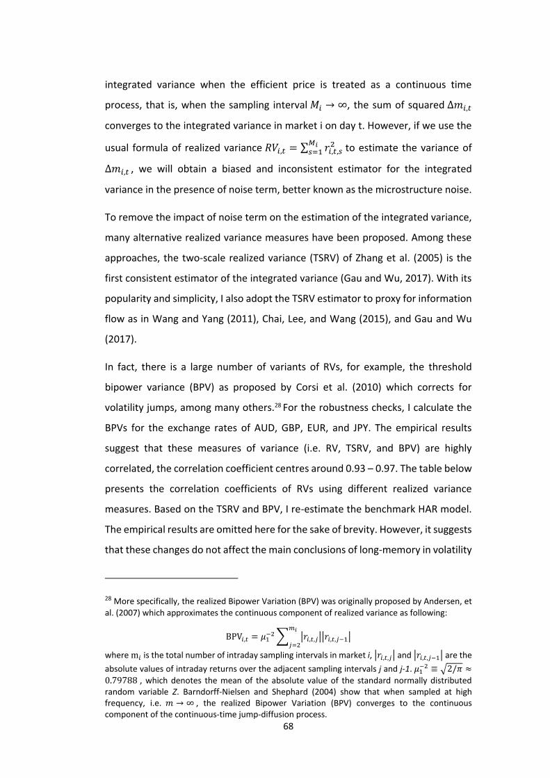
68

integrated variance when the efficient price is treated as a continuous time

process, that is, when the sampling interval 𝑀𝑖 → ∞, the sum of squared ∆𝑚𝑖,𝑡

converges to the integrated variance in market i on day t. However, if we use the

usual formula of realized variance 𝑅𝑉𝑖,𝑡 = ∑ 𝑟𝑖,𝑡,𝑠2𝑀𝑖

𝑠=1 to estimate the variance of

∆𝑚𝑖,𝑡 , we will obtain a biased and inconsistent estimator for the integrated

variance in the presence of noise term, better known as the microstructure noise.

To remove the impact of noise term on the estimation of the integrated variance,

many alternative realized variance measures have been proposed. Among these

approaches, the two-scale realized variance (TSRV) of Zhang et al. (2005) is the

first consistent estimator of the integrated variance (Gau and Wu, 2017). With its

popularity and simplicity, I also adopt the TSRV estimator to proxy for information

flow as in Wang and Yang (2011), Chai, Lee, and Wang (2015), and Gau and Wu

(2017).

In fact, there is a large number of variants of RVs, for example, the threshold

bipower variance (BPV) as proposed by Corsi et al. (2010) which corrects for

volatility jumps, among many others.28 For the robustness checks, I calculate the

BPVs for the exchange rates of AUD, GBP, EUR, and JPY. The empirical results

suggest that these measures of variance (i.e. RV, TSRV, and BPV) are highly

correlated, the correlation coefficient centres around 0.93 – 0.97. The table below

presents the correlation coefficients of RVs using different realized variance

measures. Based on the TSRV and BPV, I re-estimate the benchmark HAR model.

The empirical results are omitted here for the sake of brevity. However, it suggests

that these changes do not affect the main conclusions of long-memory in volatility

28 More specifically, the realized Bipower Variation (BPV) was originally proposed by Andersen, et al. (2007) which approximates the continuous component of realized variance as following:

BPV𝑖,𝑡 = 𝜇1−2 ∑ |𝑟𝑖,𝑡,𝑗||𝑟𝑖,𝑡,𝑗−1|

𝑚𝑖

𝑗=2

where m𝑖 is the total number of intraday sampling intervals in market i, |𝑟𝑖,𝑡,𝑗| and |𝑟𝑖,𝑡,𝑗−1| are the

absolute values of intraday returns over the adjacent sampling intervals j and j-1. 𝜇1−2 ≡ √2/𝜋 ≈

0.79788 , which denotes the mean of the absolute value of the standard normally distributed random variable Z. Barndorff-Nielsen and Shephard (2004) show that when sampled at high frequency, i.e. 𝑚 → ∞ , the realized Bipower Variation (BPV) converges to the continuous component of the continuous-time jump-diffusion process.

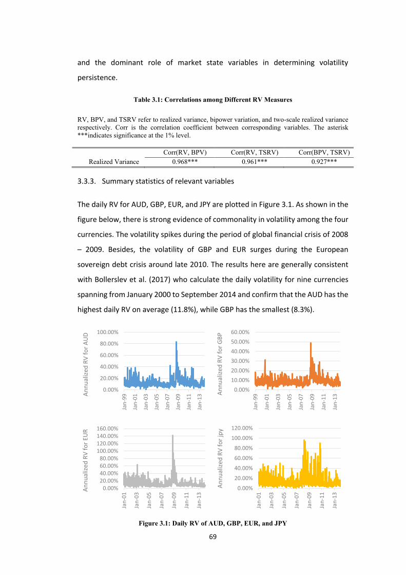
69

and the dominant role of market state variables in determining volatility

persistence.

Table 3.1: Correlations among Different RV Measures

RV, BPV, and TSRV refer to realized variance, bipower variation, and two-scale realized variance

respectively. Corr is the correlation coefficient between corresponding variables. The asterisk

***indicates significance at the 1% level.

Corr(RV, BPV) Corr(RV, TSRV) Corr(BPV, TSRV)

Realized Variance 0.968*** 0.961*** 0.927***

3.3.3. Summary statistics of relevant variables

The daily RV for AUD, GBP, EUR, and JPY are plotted in Figure 3.1. As shown in the

figure below, there is strong evidence of commonality in volatility among the four

currencies. The volatility spikes during the period of global financial crisis of 2008

– 2009. Besides, the volatility of GBP and EUR surges during the European

sovereign debt crisis around late 2010. The results here are generally consistent

with Bollerslev et al. (2017) who calculate the daily volatility for nine currencies

spanning from January 2000 to September 2014 and confirm that the AUD has the

highest daily RV on average (11.8%), while GBP has the smallest (8.3%).

Figure 3.1: Daily RV of AUD, GBP, EUR, and JPY

0.00%

20.00%

40.00%

60.00%

80.00%

100.00%

Jan

-99

Jan

-01

Jan

-03

Jan

-05

Jan

-07

Jan

-09

Jan

-11

Jan

-13A

nn

ual

ized

RV

fo

r A

UD

0.00%

10.00%

20.00%

30.00%

40.00%

50.00%

60.00%

Jan

-99

Jan

-01

Jan

-03

Jan

-05

Jan

-07

Jan

-09

Jan

-11

Jan

-13A

nn

ual

ized

RV

fo

r G

BP

0.00%20.00%40.00%60.00%80.00%

100.00%120.00%140.00%160.00%

Jan

-01

Jan

-03

Jan

-05

Jan

-07

Jan

-09

Jan

-11

Jan

-13

An

nu

aliz

ed R

V f

or

EUR

0.00%

20.00%

40.00%

60.00%

80.00%

100.00%

120.00%

Jan

-01

Jan

-03

Jan

-05

Jan

-07

Jan

-09

Jan

-11

Jan

-13

An

nu

aliz

ed R

V f

or

jpy

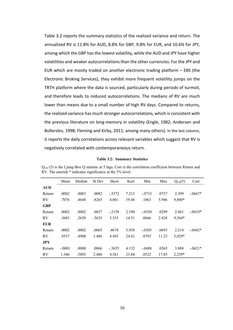
70

Table 3.2 reports the summary statistics of the realized variance and return. The

annualized RV is 11.8% for AUD, 8.8% for GBP, 9.8% for EUR, and 10.6% for JPY,

among which the GBP has the lowest volatility, while the AUD and JPY have higher

volatilities and weaker autocorrelations than the other currencies. For the JPY and

EUR which are mostly traded on another electronic trading platform – EBS (the

Electronic Broking Services), they exhibit more frequent volatility jumps on the

TRTH platform where the data is sourced, particularly during periods of turmoil,

and therefore leads to reduced autocorrelations. The medians of RV are much

lower than means due to a small number of high RV days. Compared to returns,

the realized variance has much stronger autocorrelations, which is consistent with

the previous literature on long-memory in volatility (Engle, 1982; Andersen and

Bollerslev, 1998; Fleming and Kirby, 2011; among many others). In the last column,

it reports the daily correlations across relevant variables which suggest that RV is

negatively correlated with contemporaneous return.

Table 3.2: Summary Statistics

QLB (5) is the Ljung-Box Q statistic at 5 lags. Corr is the correlation coefficient between Return and

RV. The asterisk * indicates significance at the 5% level.

Mean Median St Dev Skew Kurt Min Max QLB(5) Corr

AUD

Return .0002 .0003 .0082 -.3572 7.213 -.0733 .0737 2.399 -.0667*

RV .7076 .4648 .8265 4.001 19.48 .1063 5.946 9,800*

GBP

Return .0002 .0002 .0057 -.2158 2.190 -.0350 .0299 2.461 -.0419*

RV .3683 .2658 .3635 3.535 14.51 .0666 2.428 9,364*

EUR

Return .0002 .0002 .0065 .4678 5.938 -.0305 .0693 2.214 -.0442*

RV .9537 .4900 1.486 4.493 24.41 .0793 11.23 5,029*

JPY

Return -.0001 .0000 .0066 -.3655 4.132 -.0488 .0365 3.888 -.0621*

RV 1.346 .5892 2.486 4.561 23.84 .0522 17.85 2,259*

71

3.4. Volatility spillover in the FX market

3.4.1. Meteor showers and heat waves effects

To capture the volatility impacts from heterogeneous investors with different

trading horizons, Corsi (2009) argues that investors can be broadly classified as

trading at daily, weekly, and monthly frequencies and proposes a heterogeneous

autoregressive (HAR) model that examines differential role of three volatility

components: the daily volatility RV𝑡,𝐷 , weekly volatility RV𝑡,𝑊 , and monthly

volatility RV𝑡,𝑀 respectively. The HAR model has been applied extensively to

different financial markets, such as equity market (Andersen, Bollerslev, and

Diebold, 2007; Forsberg and Ghysels, 2007; Bollerslev et al., 2017), gold market

(Chai et al., 2015), and foreign exchange market (Wang and Yang, 2009; Wang and

Yang, 2017). In fact, Bollerslev et al. (2017) comments that the HAR model has

become “somewhat of a benchmark in the financial econometrics literature for

judging other RV–based forecasting procedures.” In this chapter, I utilize a

modified heterogeneous autoregressive (HAR) model to capture the dynamic

patterns of volatility spillovers in four trading segments as I defined earlier.

To simplify the notations, I denote 𝑅𝑉i,t by 𝑉i,t for 𝑖 = A (Asia), E (Europe), L

(London/New York) and U (US). Because volatilities are persistent, lagged

volatilities beyond one day are represented by weekly heat waves effect, that is,

the average volatility of market i over lagged 2 to 5 days, HW𝑊,𝑡−1 =1

4∑ Vi,t−k

5k=2

and monthly heat waves effect, i.e. average volatility of market i over lagged 6 to

22 days, HW𝑀,𝑡−1 =1

17∑ Vi,t−k

22k=6 . The weekly and monthly meteor showers

effects can be defined similarly, which are average volatility of market j (𝑗 ≠ 𝑖)

over lagged 2 to 5 days, MS𝑊,𝑡−1 =1

4∑ Vj,t−k

5k=2 , and over lagged 6 to 22 days,

MS𝑀,𝑡−1 =1

17∑ Vj,t−k

22k=6 , respectively. Thus, the dynamic volatility spillover

model can be written as follows:

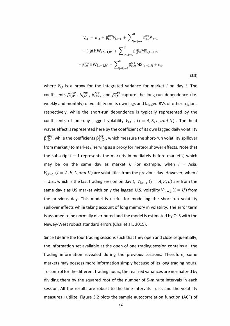
72

V𝑖,𝑡 = 𝛼𝑖,𝑡 + βi,DHW𝑉𝑖,𝑡−1 + ∑ βi,j,D

MS Vj,t−1

U

j≠i,j=A

+ βi,WHWHW𝑖,𝑡−1,𝑊 + ∑ βi,j,W

MS MS𝑖,𝑡−1,𝑊

U

j≠i,j=A

+ βi,MHWHW𝑖,𝑡−1,𝑀 + ∑ βi,j,M

MS MS𝑖,𝑡−1,𝑀

U

j≠i,j=A+ 𝜀𝑖,𝑡

(3.5)

where 𝑉𝑖,𝑡 is a proxy for the integrated variance for market i on day t. The

coefficients 𝛽𝑖,𝑊𝐻𝑊 , 𝛽𝑖,𝑀

𝐻𝑊 , 𝛽𝑖,𝑊𝑀𝑆 , and 𝛽𝑖,𝑀

𝑀𝑆 capture the long-run dependence (i.e.

weekly and monthly) of volatility on its own lags and lagged RVs of other regions

respectively, while the short-run dependence is typically represented by the

coefficients of one-day lagged volatility 𝑉𝑖,𝑡−1 (𝑖 = 𝐴, 𝐸, 𝐿, 𝑎𝑛𝑑 𝑈) . The heat

waves effect is represented here by the coefficient of its own lagged daily volatility

βi,DHW, while the coefficients βi,j,D

MS , which measure the short-run volatility spillover

from market j to market i, serving as a proxy for meteor shower effects. Note that

the subscript t − 1 represents the markets immediately before market i, which

may be on the same day as market i. For example, when i = Asia,

𝑉𝑖,𝑡−1 (𝑖 = 𝐴, 𝐸, 𝐿, 𝑎𝑛𝑑 𝑈) are volatilities from the previous day. However, when i

= U.S., which is the last trading session on day t, 𝑉𝑖,𝑡−1 (𝑖 = 𝐴, 𝐸, 𝐿) are from the

same day t as US market with only the lagged U.S. volatility 𝑉𝑖,𝑡−1 (𝑖 = 𝑈) from

the previous day. This model is useful for modelling the short-run volatility

spillover effects while taking account of long memory in volatility. The error term

is assumed to be normally distributed and the model is estimated by OLS with the

Newey-West robust standard errors (Chai et al., 2015).

Since I define the four trading sessions such that they open and close sequentially,

the information set available at the open of one trading session contains all the

trading information revealed during the previous sessions. Therefore, some

markets may possess more information simply because of its long trading hours.

To control for the different trading hours, the realized variances are normalized by

dividing them by the squared root of the number of 5-minute intervals in each

session. All the results are robust to the time intervals I use, and the volatility

measures I utilize. Figure 3.2 plots the sample autocorrelation function (ACF) of

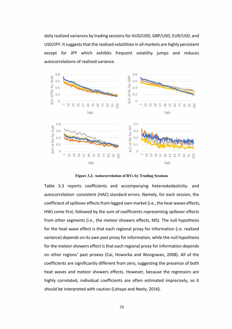
73

daily realized variances by trading sessions for AUD/USD, GBP/USD, EUR/USD, and

USD/JPY. It suggests that the realized volatilities in all markets are highly persistent

except for JPY which exhibits frequent volatility jumps and reduces

autocorrelations of realized variance.

Figure 3.2: Autocorrelation of RVs by Trading Sessions

Table 3.3 reports coefficients and accompanying heteroskedasticity- and

autocorrelation- consistent (HAC) standard errors. Namely, for each session, the

coefficient of spillover effects from lagged own market (i.e., the heat waves effects,

HW) come first, followed by the sum of coefficients representing spillover effects

from other segments (i.e., the meteor showers effects, MS). The null hypothesis

for the heat wave effect is that each regional proxy for information (i.e. realized

variance) depends on its own past proxy for information, while the null hypothesis

for the meteor showers effect is that each regional proxy for information depends

on other regions’ past proxies (Cai, Howorka and Wongswan, 2008). All of the

coefficients are significantly different from zero, suggesting the presence of both

heat waves and meteor showers effects. However, because the regressors are

highly correlated, individual coefficients are often estimated imprecisely, so it

should be interpreted with caution (Lahaye and Neely, 2016).

0

0.2

0.4

0.6

0.8

1

10

19

28

37

46

55

64

73

82

91

10

0AC

F o

f R

V f

or

AU

D

lags

0

0.2

0.4

0.6

0.8

1

10

19

28

37

46

55

64

73

82

91

10

0AC

F o

f R

v fo

r G

BP

lags

0

0.2

0.4

0.6

0.8

1

10

19

28

37

46

55

64

73

82

91

10

0AC

F o

f R

V f

or

EUR

lags

0

0.1

0.2

0.3

0.4

1

10

19

28

37

46

55

64

73

82

91

10

0

AC

F o

f R

V f

or

JPY

lags

74

Interestingly, as shown in Appendix E of sub-period analysis, the adjusted R2

increases for the regressions over the GFC period, to what a similar pattern has

been found in Wang and Yang (2017). Besides, the magnitudes of the meteor

shower and heat waves effects become larger during the global financial crisis

period (2007 - 2009). For example, the coefficients of meteor showers and heat

waves effects are significantly larger than those estimated in other periods.

The findings of increased volatility spillovers during the GFC period is consistent

with the Conditional Volatility Persistence (CVP) model where the future volatility

and its spillover varies with the market states. For example, a potential channel of

risk contagion is through the more fundamental parameters among market

participants, including changes in risk aversion and herding behaviour (Dungey et

al., 2006; W. Xiong, 2012), and the findings of increased volatility spillover during

GFC period could be attributed to the deteriorating market state (i.e. extremely

high volatility and negative returns) as a result of large exogenous information

shocks, increased risk aversion, and the herding behaviour of investors.

75

Table 3.3: Heat Waves and Meteor Showers: Full Sample

This table reports the daily persistence coefficients of the following model:


MS Vj,t−1

U

j≠i,j=A+ βi,W

HWHW𝑖,𝑡−1,𝑊 + ∑ βi,j,WMS MS𝑖,𝑡−1,𝑊

U

j≠i,j=A



U

j≠i,j=A

where i = Asia (A), Europe (E), London/NYC (L), and US (U). HW stands for daily heat waves

effect as proxied by βi,DHW, while MS stands for meteor shower effect ∑ βi,j,D

MSUj≠i,j=A (i.e., the sum of

volatility spillover effects from all other trading sessions). βi,WHW, βi,M

HW are weekly and monthly heat

waves effects, while βi,j,WMS , βi,j,M

MS are the weekly and monthly meteor shower effects respectively.

The t-statistics are calculated based on the Newey–West robust covariance with automatic lag

selection using Bartlett kernel. The asterisks ***, **, * indicate significance at 1%, 5%, and 10%

respectively.

Asia Europe London/NYC US

Coefficient t-stat Coefficient t-stat Coefficient t-stat Coefficient t-stat

AUD

𝐻𝑊 0.1544*** 6.14 0.1116*** 4.64 0.0783*** 3.57 0.1733*** 5.73

𝑀𝑆 0.4920*** 9.44 0.3687*** 12.47 0.5206*** 13.39 0.5338*** 9.13

�̅�2 .5625 .6678 .6089 .6782

GBP

𝐻𝑊 0.2220*** 6.18 0.1326*** 5.72 0.0865*** 4.41 0.1517*** 4.51

𝑀𝑆 0.4777*** 8.98 0.4506*** 10.02 0.3471*** 11.14 0.3354*** 10.25

�̅�2 .6447 .6327 .5490 .6697

EUR

𝐻𝑊 0.0983*** 2.74 0.1628*** 3.61 0.1136*** 3.82 0.0806** 2.40

𝑀𝑆 0.7856*** 4.27 0.1642*** 4.14 0.3365*** 8.34 0.8066*** 8.06

�̅�2 .3823 .6090 .4911 .4579

JPY

𝐻𝑊 0.1179*** 2.63 0.0876** 2.52 0.0705** 2.09 0.0614* 1.74

𝑀𝑆 0.4533*** 3.33 0.0913*** 3.08 0.3014*** 8.88 0.5623*** 6.93

�̅�2 .2360 .2518 .2568 .2983

3.4.2. Shapley – Owen R2 decomposition techniques

The magnitudes of the coefficients of meteor shower and heat waves effects as

shown in Table 3.3 don't explicitly suggest the relative importance of the

corresponding effects (Lahaye and Neely, 2016). For example, the individual

coefficient estimates will be conditionally marginal effects that depend on the

effects of correlated regressors, not unconditional effects. Therefore, I seek to

evaluate the importance of heat waves and meteor showers effects by adopting

other methods. In this chapter, I use the Shapley-Owen R2 measure which has its

roots in game theory, Lindeman, Merenda and Gold (1980) then apply the same

76

concepts to decompose goodness-of-fit among regressors and coalitions of

regressors in econometrics. In Lahaye and Neely (2016), the authors investigate

on the meteor shower and heat waves effects in the EUR and JPY spot rates by

utilizing the same method. Namely, the Shapley-Owen R2 measure of a group of

regressors is the average incremental improvement in R2s for each regressor (or

coalition) over all possible permutations of regressors or coalitions of regressors.29

The results of Shapley-Owen R2 values as shown in Table 3.4 suggest that the

meteor showers effect contributes more to the total variations in future volatility

compared to heat waves over daily, weekly, and monthly horizons respectively,

which is consistent with Lahaye and Neely (2014) who investigate on the EUR and

JPY spot rates and find that the meteor shower contributes 60% to the total

variations in volatility persistence, while heat waves account for the remaining

portion. Besides, the heat waves effects are relatively weaker in the LNY market

compared to other segments, which is probably due to the fact that the LNY

market is more efficient at information incorporation and contributes more to the

price discovery with large trading volume and the presence of informed traders,

resulting in low volatility spillovers to the future in the local market (Su and Zhang,

2018).

Furthermore, I conduct a subperiod analysis to examine the presence of meteor

showers and heat waves effects in different sub-periods using the same

techniques of Shapley-Owen R2 values as before. The adjusted R2 increases for the

regressions over the GFC period, to what a similar pattern has been found in Wang

and Yang (2017). Interestingly, I find that the relative importance of meteor

showers effect has been increasing rapidly and has surpassed that of heat waves

effect as shown in Table 3.5. For example, during the period of 2007 - 2009, the

meteor showers effect dominates the volatility spillovers and contributes to

around 70% of the total R2 for AUD, GBP, and EUR respectively. One possible

explanation for the dominant meteor showers effect is that the financial markets

29 For an in-detail demonstration of the Shapley-Owen R2 method, please refer to Appendix A-2 of Lahaye and Neely (2016).

77

are becoming increasingly interdependent and interconnected with financial

liberalization and market openness. On the other hand, the increasing meteor

showers effect can be seen as an indicator of the speeded-up information flow in

the FX market and the internationalization of currencies. For example, Evans and

Lyons (2002) find strong evidence of a high degree of informational integration in

international money markets.

The potential adverse effects of volatility spillover on financial stability,

particularly during periods of high uncertainty, is a subject of great importance in

the current context of increasing financial integration (Boucher et al., 2016).

Interestingly, the results in Table 3.5 suggest that the meteor shower effects

become particularly strong on high volatility days (i.e. during the GFC period). High

volatility reflects high uncertainty which takes longer to be resolved, while high

volatility is generally associated with greater volatility spillovers across regions, an

interesting question that is worth exploring in the future.

78

Table 3.4: Shapley-Owen R2 Values: Full Sample

This table shows the Shapley-Owen proportion of the total R2s in four trading sessions (Asia, Europe,

LNY, and US). The calculation is based on Eq. (3.5). Namely, there are 2 groups of coefficients: the

heat wave (HW) contribution, which includes the daily, weekly, and monthly own lags of RV, and

the meteor shower (MS) counterparts. Normal and High stands for the days with normal and extreme

volatilities respectively as defined in Section 3.4.2. The groups have no intersection and include all

non-deterministic regressors, so the proportions for each intraday period sum to one.

Asia Europe LNY US Average

AUD

Daily HW 0.10 0.09 0.08 0.10 0.09

MS 0.26 0.25 0.27 0.24 0.26

Weekly HW 0.14 0.13 0.16 0.10 0.13

MS 0.23 0.22 0.22 0.23 0.22

Monthly HW 0.09 0.10 0.09 0.10 0.09

MS 0.19 0.21 0.19 0.22 0.20

Total HW 0.32 0.32 0.22 0.31 0.32

MS 0.68 0.68 0.78 0.69 0.68

GBP

Daily HW 0.12 0.08 0.07 0.10 0.09

MS 0.25 0.23 0.25 0.25 0.24

Weekly HW 0.12 0.11 0.10 0.09 0.11

MS 0.24 0.24 0.25 0.25 0.25

Monthly HW 0.07 0.09 0.09 0.08 0.08

MS 0.21 0.24 0.24 0.23 0.23

Total HW 0.30 0.29 0.26 0.27 0.28

MS 0.70 0.71 0.74 0.73 0.72

EUR

Daily HW 0.08 0.11 0.09 0.07 0.09

MS 0.24 0.26 0.25 0.25 0.25

Weekly HW 0.16 0.06 0.17 0.10 0.12

MS 0.22 0.29 0.21 0.24 0.24

Monthly HW 0.04 0.04 0.06 0.10 0.06

MS 0.25 0.25 0.22 0.24 0.24

Total HW 0.28 0.21 0.22 0.27 0.27

MS 0.72 0.79 0.78 0.73 0.73

JPY

Daily HW 0.13 0.07 0.04 0.03 0.07

MS 0.24 0.19 0.12 0.30 0.21

Weekly HW 0.12 0.34 0.51 0.20 0.30

MS 0.26 0.20 0.12 0.23 0.20

Monthly HW 0.02 0.04 0.11 0.06 0.06

MS 0.24 0.15 0.10 0.18 0.17

Total HW 0.26 0.46 0.33 0.29 0.42

MS 0.74 0.54 0.67 0.71 0.58

79

Table 3.5: Shapley-Owen R2 Values: Sub-periods

This table shows the Shapley-Owen proportion of the total R2s in four trading sessions (i.e., Asia,

Europe, LNY, and US), for groups of coefficients in the HAR model where RV is predicted by

lagged RVs, in different sub-periods. There are 2 groups of coefficients: the heat waves (HW)

contribution, which includes the daily, weekly, and monthly components of own lags of RV, and the

meteor shower (MS) counterparts. The groups have no intersection and include all non-deterministic

regressors, so the proportions of HW and MS effects for each trading session sum to one.

Asia Europe London/NYC US Average

AUD

1999 – 2006

𝐻𝑊 0.49 0.47 0.40 0.54 0.48

𝑀𝑆 0.51 0.53 0.60 0.46 0.52

2007 – 2009

𝐻𝑊 0.34 0.34 0.33 0.30 0.33

𝑀𝑆 0.66 0.66 0.67 0.70 0.67

2010 – 2013

𝐻𝑊 0.31 0.25 0.38 0.50 0.36

𝑀𝑆 0.69 0.75 0.62 0.50 0.64

GBP

1999 – 2006

𝐻𝑊 0.35 0.42 0.27 0.47 0.38

𝑀𝑆 0.65 0.58 0.73 0.53 0.62

2007 – 2009

𝐻𝑊 0.35 0.29 0.27 0.27 0.30

𝑀𝑆 0.65 0.71 0.73 0.73 0.70

2010 – 2013

𝐻𝑊 0.37 0.39 0.34 0.36 0.37

𝑀𝑆 0.63 0.61 0.66 0.64 0.63

EUR

2000 - 2006

𝐻𝑊 0.42 0.37 0.49 0.42 0.43

𝑀𝑆 0.58 0.63 0.51 0.58 0.57

2007 – 2009

𝐻𝑊 0.29 0.22 0.30 0.26 0.27

𝑀𝑆 0.71 0.78 0.70 0.74 0.73

2010 - 2013

𝐻𝑊 0.30 0.25 0.40 0.39 0.34

𝑀𝑆 0.70 0.75 0.60 0.61 0.66

JPY

1999 - 2006

𝐻𝑊 0.72 0.57 0.68 0.34 0.58

𝑀𝑆 0.28 0.43 0.32 0.66 0.42

2007 – 2009

𝐻𝑊 0.17 0.63 0.71 0.61 0.53

𝑀𝑆 0.83 0.37 0.29 0.39 0.47

2010 - 2013

𝐻𝑊 0.22 0.53 0.69 0.18 0.40

𝑀𝑆 0.78 0.47 0.31 0.82 0.60

80

3.5. Determinants of Volatility Spillover

3.5.1. Conditional Volatility Persistence Model (CVP)

As stated earlier, I propose that volatility persistence is driven by the nature,

precision, and volume of both exogenous and endogenous information arrivals. It

is also driven by uninformed trading such as portfolio adjustments to lagged

information shocks. Collectively these mechanisms determine the state of the

market, and in turn, volatility persistence. Through the above-mentioned channels,

I introduce the Conditional Volatility Persistence (CVP) model as proposed in Wang

and Yang (2017), which captures the long memory in volatility while controlling

for conditional variables (i.e., return, volatility, and other proxies for trading

activities).

Namely, to examine the determinants of volatility spillover, I incorporate time-

varying volatility persistence into the HAR model, i.e., the HAR-CVP model. Here,

considering that the negative returns are generally associated with greater

volatility than positive returns in the equity market (Patton and Sheppard, 2006),

and in the FX market (Wang and Yang, 2009), I decompose exchange rate returns

into positive and negative returns, and examine their volatility impacts separately.

Specifically, I extend the HAR model in a multi-market setting and examine the

heterogeneous effects of market state variables in different FX trading sessions as

follows:

𝑅𝑉𝑖,𝑡 = 𝛼𝑖,𝑡 + 𝛽𝐴,𝑡𝑒 𝑅𝑉𝐴,𝑡−1 + 𝛽𝐸,𝑡

𝑒 𝑅𝑉𝐸,𝑡−1 + 𝛽𝐿,𝑡𝑒 𝑅𝑉𝐿,𝑡−1 + 𝛽𝑈,𝑡

𝑒 𝑅𝑉𝑈,𝑡−1 + βi,WHWRV̅̅ ̅̅

i,t−1,W +

∑ βi,j,WMS RV̅̅ ̅̅

j,t−1,WUj≠i,j=A + βi,M

HWRV̅̅ ̅̅i,t−1,M + ∑ βi,j,M

MS RV̅̅ ̅̅j,t−1,M

Uj≠i,j=A + 𝜀𝑖,𝑡 (3.6)

where 𝑅𝑉𝑖,𝑡 stands for the realized variance (RV) for market i on day t. The

coefficients of 𝛽𝑖,𝑊𝐻𝑊, 𝛽𝑖,𝑀

𝐻𝑊, 𝛽𝑖,𝑗,𝑊𝑀𝑆 , and 𝛽𝑖,𝑗,𝑀

𝑀𝑆 capture the long-run dependence of

volatility on its own lagged market and other markets respectively. Here, the

short-run dependence is represented by the time-varying coefficients of one-day

lagged volatility 𝛽𝑗,𝑡𝑒 (𝑖 = 𝐴, 𝐸, 𝐿, 𝑎𝑛𝑑 𝑈) , namely, 𝛽𝑗,𝑡

𝑒 = 𝛽 + 𝛽−𝑟𝑗,𝑡−1− + 𝛽+𝑟𝑗,𝑡−1

+ +

𝛽𝑅𝑉𝑅𝑉𝑗,𝑡−1 (𝑗 = 𝐴, 𝐸, 𝐿, 𝑎𝑛𝑑 𝑈) is the conditional volatility spillover from market j

to market i , which depends on the lagged market state variables as defined earlier.

The meteor shower effects are defined as the volatility spillovers from other

81

segments 𝛽𝑗,𝑡𝑒 (𝑗 ≠ 𝑖), while heat waves effects are represented by the volatility

persistence within the local segment 𝛽𝑗,𝑡𝑒 (𝑗 = 𝑖) . The use of return and volatility

as the state variables is in the same spirit as Campbell and Hentschel (1992) and

Wu (2001) who use dividend shock and dividend volatility as the state variables to

explain the asymmetric return impact on volatility. I also test the impacts of other

market state variables on volatility persistence, e.g. liquidity, trading volume, etc.,

in the robustness section.

Furthermore, to relate the volatility spillovers model to the information-based

explanations, I explore the impacts of price discovery on the volatility spillover.

Namely, considering the fact that daily volatility often has an information flow

interpretation (Andersen, 1996) and a popular measure for price discovery is the

variance of the random-walk return component (Hasbrouck, 1995), I utilize the

information share (i.e. realized variance ratio) as a measure of price discovery (Gau

and Wu, 2017; Su and Zhang, 2018).30 The empirical results in Wang and Yang

(2017) suggest that the price discovery plays a key role in determining the time-

varying volatility persistence, and more price discovery increases the information

content of quoted price and reduces the spillovers of uncertainty over time. Thus,

I utilize the information share as a proxy for price discovery process and explicitly

explore its role in volatility spillovers in different trading sessions. In fact, the

information interpretation of daily volatility is supported by the MDH theory, e.g.

Andersen (1996), and the microstructure literature where price discovery is

measured as the variance of the random walk component of return, e.g.

Hasbrouck (1995). The summary statistics of information share as shown in

Appendix G suggest that the European market contributes the most to the price

discovery, while the LNY market dominates the price discovery process on a per

hour basis.31

30 Using volatility to proxy for information has some advantages over using returns (Cai, et al., 2008). Firstly, the volatility is more persistent and therefore inherently easier to forecast. Furthermore, volatility is more closely related to information. For example, Wang and Yang (2017) argue that even though the absolute return has been used in many studies as a proxy for return standard deviation, the absolute return is not a robust measure of return uncertainty. 31 The high information share of the LNY market is also possibly attributed to the timing of release of macroeconomic news announcements on the U.S. economy as the market becomes relatively

82

To conserve space, I don’t report all the coefficient estimates from the four-

market equations. Instead I present the Wald statistics and the corresponding p-

values. As reported in Column (1) of Panel A of Table 3.6, the null hypotheses that

𝛽− = 𝛽+ = 𝛽𝑅𝑉 = 0 are resoundingly rejected at the 5% significance level, which

confirm the explanatory power of market state variable in explaining volatility

spillovers. Furthermore, the null hypotheses that 𝛽− = 𝛽+ = 𝛽𝑅𝑉 = 𝛽𝐼𝑆 = 0 are

examined by adding the information share as one of market state variables in the

conditional volatility persistence 𝛽𝑗,𝑡𝑒 as documented in Eq. (3.6). The empirical

results in Panel A of Table 3.6 can be interpreted as following: Firstly, comparing

the overall explanatory power of models as shown in Table 3.3 and Table 3.6, the

adjusted R-squared are in favour of the extended HAR model specification over

the regular one which ignores the role of changing market states in explaining

volatility persistence. Secondly, the inclusion of variance ratio increases the model

performance and deepens our understanding of the economic mechanisms of

volatility spillovers in the FX market (i.e. either the adjusted R-squared or the

Wald-statistics suggests the superior performance when including the information

share). Furthermore, I report a summary of the sign and significance of CVP

variables. Namely, Panel B of Table 3.6 reports the number of significantly positive

(negative) coefficients of market state variables (i.e., including the constant,

positive\negative return, volatility, and information share) which presents

evidence on individual coefficients without reporting all coefficients. The result

suggests that most of the coefficients of negative (positive) return are negatively

(positively) significant, which is consistent with the previous findings on

asymmetric effect, while the coefficients of RV are generally negatively significant,

suggesting a reduction in volatility spillover on days of high volatility. Furthermore,

most of the coefficients of information share are negatively significant, suggesting

that the price discovery has a dampening effect on the volatility spillover. With

high information shares, the market contributes more to the price discovery

process, which helps in reducing the uncertainty and mitigating the propagation

more efficient in reflecting information when more macro news announcements are released during its trading hours (Su and Zhang, 2018). The gain in information share when public information is released is also consistent with the findings of Jiang, et al. (2014).

83

of volatility. Besides, including information share as the market state variable

slightly weakens the statistical significance of other market state variable and

decreases the volatility persistence as measured by the coefficient β𝑗0. Overall, the

inclusion of information share significantly improves the model performance and

provides information-based explanations by relating the time-varying volatility

spillovers in the FX market to the price discovery process.

Furthermore, I explore the differential role of market state variables in predicting

the future volatility by utilizing the Shapley-Owen R2 Decomposition techniques.

Namely, I assess the importance of conditional volatility persistence (CVP) by

computing the Shapley-Owen values in the HAR-CVP models. Panel C of Table 3.6

reports the Shapley-Owen values of each market state variable in explaining the

inter- and intra-regional volatility spillover (i.e. meteor showers and heat waves

effects) which confirms the relatively important role of market state variable in

predicting the future volatility in different regions. For example, the ratio of

Shapley-Owen value of 𝛽0 to the CVP ranges from 39% to 44%, indicating that the

conventional measure of volatility persistence in each region, as proxied by 𝛽0,

decreases substantially after controlling for the market state variables, while the

groups of market state variables contribute to more than half of the explanatory

powers in conditional volatility spillover. Overall, the CVP variable has the highest

Shapley-Owen R2 values across all explanatory variables. The Shapley-Owen R2

values of market state variables sum to around 0.6, suggesting that roughly 60%

of the explanatory power of RV𝑡 in the traditional HAR model comes from the

omitted CVP variables. Furthermore, the negative return, positive return, volatility,

and information share explains around 8%, 7%, 23%, and 20% of the total

variations in conditional volatility persistence respectively, among which the

volatility and variance ratio explains most of the total variations in time-varying

volatility spillover. Besides, negative return plays a slightly more important role

than positive return, confirming the weak asymmetric effects as documented

earlier. However, for each market state variable, I don’t find their differential roles

in explaining the meteor showers and heat waves effects. Overall, the

consideration of market state variables significantly depends our understanding

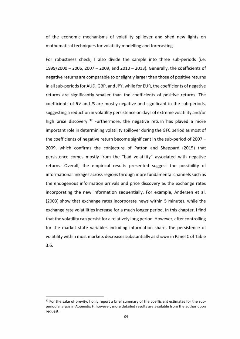
84

of the economic mechanisms of volatility spillover and shed new lights on

mathematical techniques for volatility modelling and forecasting.

For robustness check, I also divide the sample into three sub-periods (i.e.

1999/2000 – 2006, 2007 – 2009, and 2010 – 2013). Generally, the coefficients of

negative returns are comparable to or slightly larger than those of positive returns

in all sub-periods for AUD, GBP, and JPY, while for EUR, the coefficients of negative

returns are significantly smaller than the coefficients of positive returns. The

coefficients of RV and IS are mostly negative and significant in the sub-periods,

suggesting a reduction in volatility persistence on days of extreme volatility and/or

high price discovery. 32 Furthermore, the negative return has played a more

important role in determining volatility spillover during the GFC period as most of

the coefficients of negative return become significant in the sub-period of 2007 –

2009, which confirms the conjecture of Patton and Sheppard (2015) that

persistence comes mostly from the “bad volatility” associated with negative

returns. Overall, the empirical results presented suggest the possibility of

informational linkages across regions through more fundamental channels such as

the endogenous information arrivals and price discovery as the exchange rates

incorporating the new information sequentially. For example, Andersen et al.

(2003) show that exchange rates incorporate news within 5 minutes, while the

exchange rate volatilities increase for a much longer period. In this chapter, I find

that the volatility can persist for a relatively long period. However, after controlling

for the market state variables including information share, the persistence of

volatility within most markets decreases substantially as shown in Panel C of Table

3.6.

32 For the sake of brevity, I only report a brief summary of the coefficient estimates for the sub-period analysis in Appendix F, however, more detailed results are available from the author upon request.

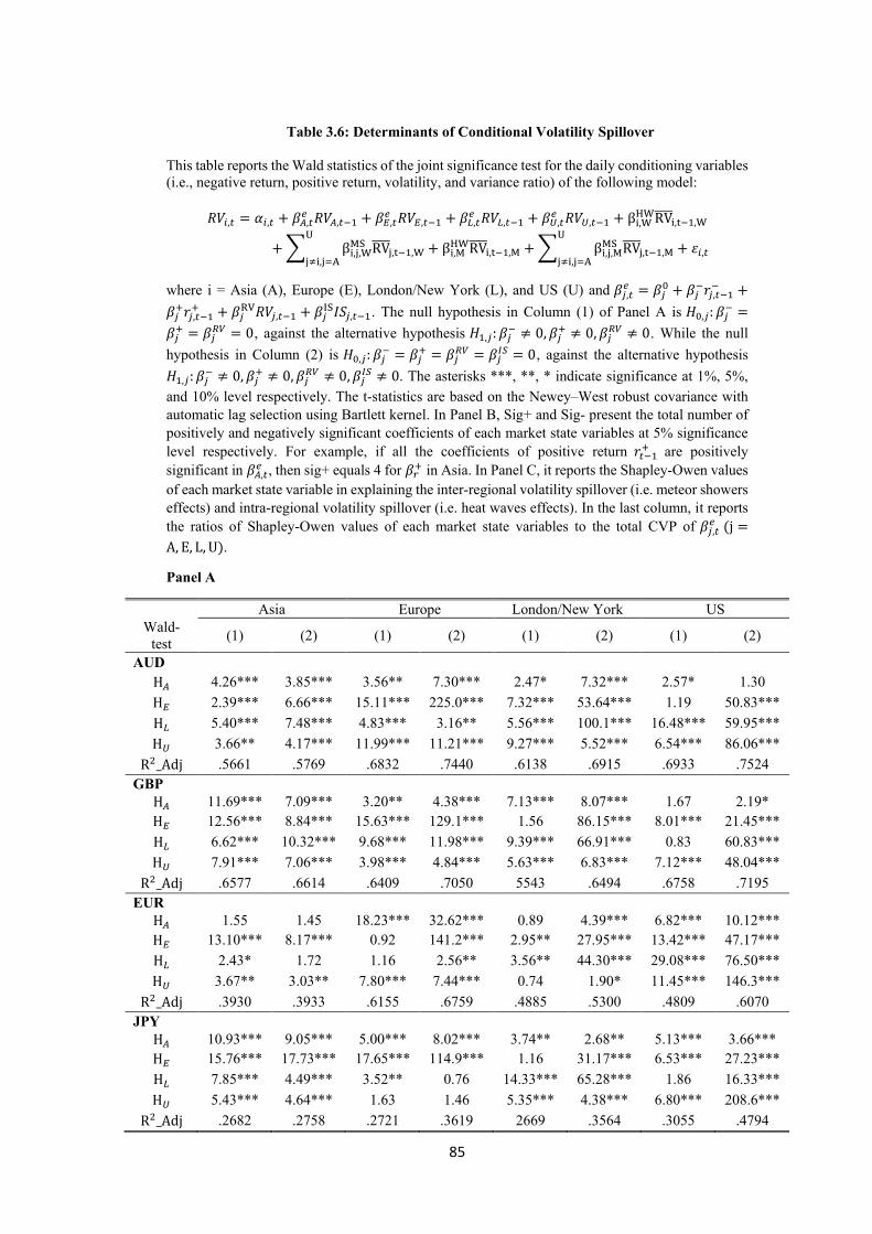
85

Table 3.6: Determinants of Conditional Volatility Spillover

This table reports the Wald statistics of the joint significance test for the daily conditioning variables

(i.e., negative return, positive return, volatility, and variance ratio) of the following model:




i,t−1,W

+ ∑ βi,j,WMS RV̅̅ ̅̅

j,t−1,W

U

j≠i,j=A+ βi,M



U


where i = Asia (A), Europe (E), London/New York (L), and US (U) and 𝛽𝑗,𝑡𝑒 = 𝛽𝑗

0 + 𝛽𝑗−𝑟𝑗,𝑡−1

− +

𝛽𝑗+𝑟𝑗,𝑡−1

+ + 𝛽𝑗RV𝑅𝑉𝑗,𝑡−1 + 𝛽𝑗

IS𝐼𝑆𝑗,𝑡−1. The null hypothesis in Column (1) of Panel A is 𝐻0,𝑗: 𝛽𝑗− =

𝛽𝑗+ = 𝛽𝑗

𝑅𝑉 = 0, against the alternative hypothesis 𝐻1,𝑗: 𝛽𝑗− ≠ 0, 𝛽𝑗

+ ≠ 0, 𝛽𝑗𝑅𝑉 ≠ 0. While the null

hypothesis in Column (2) is 𝐻0,𝑗: 𝛽𝑗− = 𝛽𝑗

+ = 𝛽𝑗𝑅𝑉 = 𝛽𝑗

𝐼𝑆 = 0, against the alternative hypothesis

𝐻1,𝑗: 𝛽𝑗− ≠ 0, 𝛽𝑗

+ ≠ 0, 𝛽𝑗𝑅𝑉 ≠ 0, 𝛽𝑗

𝐼𝑆 ≠ 0. The asterisks ***, **, * indicate significance at 1%, 5%,

and 10% level respectively. The t-statistics are based on the Newey–West robust covariance with

automatic lag selection using Bartlett kernel. In Panel B, Sig+ and Sig- present the total number of

positively and negatively significant coefficients of each market state variables at 5% significance

level respectively. For example, if all the coefficients of positive return 𝑟𝑡−1+ are positively

significant in 𝛽𝐴,𝑡𝑒 , then sig+ equals 4 for 𝛽𝑟

+ in Asia. In Panel C, it reports the Shapley-Owen values

of each market state variable in explaining the inter-regional volatility spillover (i.e. meteor showers

effects) and intra-regional volatility spillover (i.e. heat waves effects). In the last column, it reports

the ratios of Shapley-Owen values of each market state variables to the total CVP of 𝛽𝑗,𝑡𝑒 (j =

A, E, L, U).

Panel A

Asia Europe London/New York US

Wald-

test (1) (2) (1) (2) (1) (2) (1) (2)

AUD

H𝐴 4.26*** 3.85*** 3.56** 7.30*** 2.47* 7.32*** 2.57* 1.30

H𝐸 2.39*** 6.66*** 15.11*** 225.0*** 7.32*** 53.64*** 1.19 50.83***

H𝐿 5.40*** 7.48*** 4.83*** 3.16** 5.56*** 100.1*** 16.48*** 59.95***

H𝑈 3.66** 4.17*** 11.99*** 11.21*** 9.27*** 5.52*** 6.54*** 86.06***

R2_Adj .5661 .5769 .6832 .7440 .6138 .6915 .6933 .7524

GBP

H𝐴 11.69*** 7.09*** 3.20** 4.38*** 7.13*** 8.07*** 1.67 2.19*

H𝐸 12.56*** 8.84*** 15.63*** 129.1*** 1.56 86.15*** 8.01*** 21.45***

H𝐿 6.62*** 10.32*** 9.68*** 11.98*** 9.39*** 66.91*** 0.83 60.83***

H𝑈 7.91*** 7.06*** 3.98*** 4.84*** 5.63*** 6.83*** 7.12*** 48.04***

R2_Adj .6577 .6614 .6409 .7050 5543 .6494 .6758 .7195

EUR

H𝐴 1.55 1.45 18.23*** 32.62*** 0.89 4.39*** 6.82*** 10.12***

H𝐸 13.10*** 8.17*** 0.92 141.2*** 2.95** 27.95*** 13.42*** 47.17***

H𝐿 2.43* 1.72 1.16 2.56** 3.56** 44.30*** 29.08*** 76.50***

H𝑈 3.67** 3.03** 7.80*** 7.44*** 0.74 1.90* 11.45*** 146.3***

R2_Adj .3930 .3933 .6155 .6759 .4885 .5300 .4809 .6070

JPY

H𝐴 10.93*** 9.05*** 5.00*** 8.02*** 3.74** 2.68** 5.13*** 3.66***

H𝐸 15.76*** 17.73*** 17.65*** 114.9*** 1.16 31.17*** 6.53*** 27.23***

H𝐿 7.85*** 4.49*** 3.52** 0.76 14.33*** 65.28*** 1.86 16.33***

H𝑈 5.43*** 4.64*** 1.63 1.46 5.35*** 4.38*** 6.80*** 208.6***

R2_Adj .2682 .2758 .2721 .3619 2669 .3564 .3055 .4794

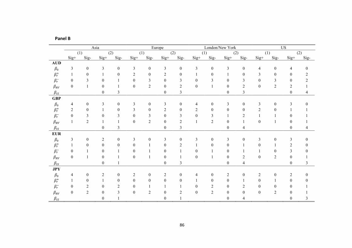
86

Panel B

Asia Europe London/New York US

(1) (2) (1) (2) (1) (2) (1) (2)

Sig+ Sig- Sig+ Sig- Sig+ Sig- Sig+ Sig- Sig+ Sig- Sig+ Sig- Sig+ Sig- Sig+ Sig-

AUD

𝛽0 3 0 3 0 3 0 3 0 3 0 3 0 4 0 4 0

𝛽𝑟+ 1 0 1 0 2 0 2 0 1 0 1 0 3 0 0 2

𝛽𝑟− 0 3 0 1 0 3 0 3 0 3 0 3 0 3 0 2

𝛽𝑅𝑉 0 1 0 1 0 2 0 2 0 1 0 2 0 2 2 1

𝛽𝐼𝑆 0 3 0 3 0 3 0 4

GBP

𝛽0 4 0 3 0 3 0 3 0 4 0 3 0 3 0 3 0

𝛽𝑟+ 2 0 1 0 3 0 2 0 2 0 0 0 2 0 1 1

𝛽𝑟− 0 3 0 3 0 3 0 3 0 3 1 2 1 1 0 1

𝛽𝑅𝑉 1 2 1 1 0 2 0 2 1 2 0 1 0 1 0 1

𝛽𝐼𝑆 0 3 0 3 0 4 0 4

EUR

𝛽0 3 0 2 0 3 0 3 0 3 0 3 0 3 0 3 0

𝛽𝑟+ 1 0 0 0 0 1 0 2 1 0 0 1 0 1 2 0

𝛽𝑟− 0 1 0 1 0 1 0 1 0 1 0 1 1 0 3 0

𝛽𝑅𝑉 0 1 0 1 0 1 0 1 0 1 0 2 0 2 0 1

𝛽𝐼𝑆 0 1 0 3 0 4 0 3

JPY

𝛽0 4 0 2 0 2 0 2 0 4 0 2 0 2 0 2 0

𝛽𝑟+ 1 0 1 0 0 0 0 0 1 0 0 1 0 1 0 0

𝛽𝑟− 0 2 0 2 0 1 1 1 0 2 0 2 0 0 0 1

𝛽𝑅𝑉 0 2 0 3 0 2 0 2 0 2 0 0 0 2 0 1

𝛽𝐼𝑆 0 1 0 1 0 4 0 3

87

Panel C

Asia Europe LNY US 𝛽𝑖/𝐶𝑉𝑃

AUD

𝛽𝑟−

HW 0.02 0.01 0.02 0.02 9.34%

𝑀𝑆 0.06 0.07 0.06 0.05

𝛽𝑟+

HW 0.02 0.01 0.01 0.01 6.33%

𝑀𝑆 0.04 0.03 0.05 0.04

𝛽𝑅𝑉 HW 0.05 0.05 0.04 0.06

26.20% 𝑀𝑆 0.18 0.15 0.16 0.18

𝛽𝐼𝑆 HW 0.04 0.02 0.02 0.03

17.47% 𝑀𝑆 0.09 0.12 0.14 0.12

𝛽0 HW 0.07 0.08 0.06 0.08

40.66% 𝑀𝑆 0.26 0.27 0.29 0.24

GBP

𝛽𝑟−

HW 0.02 0.02 0.01 0.01 8.72%

𝑀𝑆 0.06 0.06 0.05 0.05

𝛽𝑟+

HW 0.02 0.01 0.01 0.02 7.48%

𝑀𝑆 0.04 0.05 0.05 0.04

𝛽𝑅𝑉 HW 0.06 0.05 0.04 0.06

27.41% 𝑀𝑆 0.17 0.16 0.16 0.18

𝛽𝐼𝑆 HW 0.05 0.03 0.02 0.03

17.76% 𝑀𝑆 0.08 0.11 0.14 0.11

𝛽0 HW 0.09 0.08 0.06 0.07

38.63% 𝑀𝑆 0.21 0.24 0.27 0.22

EUR

𝛽𝑟−

HW 0.01 0.02 0.01 0.01 6.25%

𝑀𝑆 0.03 0.04 0.04 0.03

𝛽𝑟+

HW 0.02 0.01 0.01 0.01 8.55%

𝑀𝑆 0.06 0.04 0.04 0.07

𝛽𝑅𝑉 HW 0.04 0.06 0.05 0.03

23.03% 𝑀𝑆 0.12 0.12 0.14 0.14

𝛽𝐼𝑆 HW 0.04 0.04 0.02 0.02

20.07% 𝑀𝑆 0.10 0.09 0.12 0.18

𝛽0 HW 0.08 0.10 0.08 0.05

42.11% 𝑀𝑆 0.24 0.19 0.27 0.27

JPY

𝛽𝑟−

HW 0.04 0.01 0.01 0.01 7.59%

𝑀𝑆 0.08 0.02 0.04 0.03

𝛽𝑟+

HW 0.01 0.01 0.01 0.01 5.70%

𝑀𝑆 0.03 0.03 0.04 0.04

𝛽𝑅𝑉 HW 0.05 0.02 0.01 0.01

16.77% 𝑀𝑆 0.07 0.09 0.16 0.12

𝛽𝐼𝑆 HW 0.06 0.02 0.01 0.01

25.95% 𝑀𝑆 0.08 0.19 0.20 0.25

𝛽0 HW 0.08 0.05 0.02 0.02

43.99% 𝑀𝑆 0.13 0.35 0.41 0.33

88

To sum up, the empirical results suggest the dominant role of conditional volatility

persistence in linking changing market states to future volatility and its spillover.

Importantly, this study makes several contributions to the literature on volatility

spillover and information propagation. For example, I confirm that it is not only

the exogeneous information arrival (i.e. release of macroeconomic news) that can

cause the volatility spillover, but also the endogenous information arrival and

information propagation, which probably involves information searching, price

discovery, and strategic trading. For a big information shock, it may take a few

days, even a few weeks to be fully incorporated into the price, which is capable to

induce volatility spillovers even without new incoming information, that is, a

significant departure from the previous literature which essentially ignore the role

of endogenous information arrival and price discovery in volatility spillover. Last

but not least, this study has important practical implications as well. For example,

volatility model which explicitly takes into account the characteristics of

conditional volatility persistence can achieve superior forecasting performance

and therefore generate moderate economic gains (Su, 2017).

3.5.2. Intraday pattern of volatility spillover

In this section, I calculate the magnitudes of daily conditional volatility spillovers

as follows: 𝐶𝑉�̂�𝑖,𝑡 = �̂�0 + �̂�−𝑟𝑡− + �̂�+𝑟𝑡

+ + �̂�𝑅𝑉𝑅𝑉𝑡 + �̂�𝐼𝑆𝐼𝑆𝑡 (i =

𝐴𝑠𝑖𝑎, 𝐸𝑢𝑟𝑜𝑝𝑒, 𝐿𝑁𝑌, 𝑎𝑛𝑑 𝑈𝑆) for different trading sessions. 𝐶𝑉�̂� are very high in

all markets, particularly during the financial crisis in the second half of 2008. There

are a few 𝐶𝑉�̂�, either larger than one or smaller than 0. The mean and standard

deviation of the estimated 𝐶𝑉�̂� for each trading session of AUD, GBP, EUR, and

JPY are reported in Table 3.7. The values on the diagonal in each panel reports the

summary statistics of local-market effect (i.e., heat waves effect), while the off-

diagonal elements of each panel represent the cross-market effects (i.e., meteor

showers effect). Overall, there is considerable support for the presence of meteor

showers and heat waves effects since most of the values are statistically different

from zero. The findings of Table 3.7 also confirm the “information dominance”

that the FX microstructure literature has highlighted: information shocks from

89

some regions are more important than others (Evans and Lyons, 2001). The

evidence indicates that volatility from Europe is an important source of volatility

shocks for LNY market, while the volatility from LNY spills over to all other markets.

Besides, volatility emanating from Asia is more relevant for JPY than for AUD.

I also report the correlations of 𝐶𝑉�̂� with other variables in Table 4.6 of Chapter

4. 𝐶𝑉�̂� is significantly and negatively correlated with return, which is consistent

with the large impacts from negative returns. Besides, the unconditional

correlation between 𝐶𝑉�̂� and RV is positive. Furthermore, 𝐶𝑉�̂� is highly

persistent (i.e. the Ljung-Box statistics are all statistically significant at the 5%

significance level) but is less persistent than RV as indicated by the Ljung-Box

statistics.

Besides, under the model specification of HAR-CVP model, to measure the relative

importance of volatility spillover effects from different trading sessions in

predicting future volatility, I utilize the techniques of Shapley-Owen R2 values,

which proves to be a more efficient estimator as stated earlier. Interestingly, the

results as shown in Table 3.8 suggest that the meteor shower effect, especially the

volatility spillover effect from the preceding market, contributes most to the total

variations in future volatility, which is in accordance with the results of Table 3.7.

However, the volatility from Asia contributes a significant proportion of the total

variations in the time-varying volatility persistence for AUD, which is consistent

with the findings of Su and Zhang (2018) which suggest that the Asia contributes

more to the price discovery for AUD trading even with its declining market shares

compared to Europe and U.S.

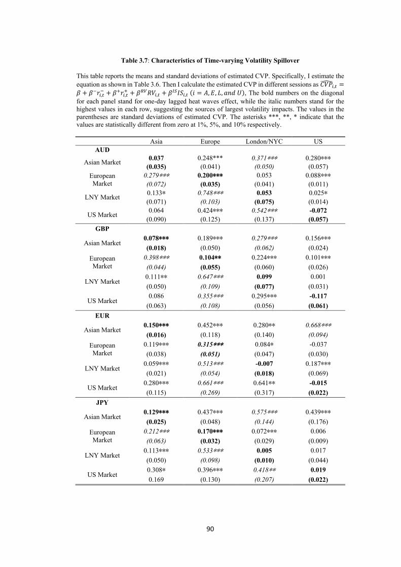
90

Table 3.7: Characteristics of Time-varying Volatility Spillover

This table reports the means and standard deviations of estimated CVP. Specifically, I estimate the

equation as shown in Table 3.6. Then I calculate the estimated CVP in different sessions as 𝐶𝑉�̂�𝑖,𝑡 =

𝛽 + 𝛽−𝑟𝑖,𝑡− + 𝛽+𝑟𝑖,𝑡

+ + 𝛽𝑅𝑉𝑅𝑉𝑖,𝑡 + 𝛽𝐼𝑆𝐼𝑆𝑖,𝑡 (𝑖 = 𝐴, 𝐸, 𝐿, 𝑎𝑛𝑑 𝑈), The bold numbers on the diagonal

for each panel stand for one-day lagged heat waves effect, while the italic numbers stand for the

highest values in each row, suggesting the sources of largest volatility impacts. The values in the

parentheses are standard deviations of estimated CVP. The asterisks ***, **, * indicate that the

values are statistically different from zero at 1%, 5%, and 10% respectively.


AUD

Asian Market 0.037 0.248*** 0.371*** 0.280***

(0.035) (0.041) (0.050) (0.057)

European

Market

0.279*** 0.200*** 0.053 0.088***

(0.072) (0.035) (0.041) (0.011)

LNY Market 0.133* 0.748*** 0.053 0.025*

(0.071) (0.103) (0.075) (0.014)

US Market 0.064 0.424*** 0.542*** -0.072

(0.090) (0.125) (0.137) (0.057)

GBP

Asian Market 0.078*** 0.189*** 0.279*** 0.156***

(0.018) (0.050) (0.062) (0.024)

European

Market

0.398*** 0.104** 0.224*** 0.101***

(0.044) (0.055) (0.060) (0.026)

LNY Market 0.111** 0.647*** 0.099 0.001

(0.050) (0.109) (0.077) (0.031)

US Market 0.086 0.355*** 0.295*** -0.117

(0.063) (0.108) (0.056) (0.061)

EUR

Asian Market 0.150*** 0.452*** 0.280** 0.668***

(0.016) (0.118) (0.140) (0.094)

European

Market

0.119*** 0.315*** 0.084* -0.037

(0.038) (0.051) (0.047) (0.030)

LNY Market 0.059*** 0.513*** -0.007 0.187***

(0.021) (0.054) (0.018) (0.069)

US Market 0.280*** 0.661*** 0.641** -0.015

(0.115) (0.269) (0.317) (0.022)

JPY

Asian Market 0.129*** 0.437*** 0.575*** 0.439***

(0.025) (0.048) (0.144) (0.176)

European

Market

0.212*** 0.170*** 0.072*** 0.006

(0.063) (0.032) (0.029) (0.009)

LNY Market 0.113*** 0.533*** 0.005 0.017

(0.050) (0.098) (0.010) (0.044)

US Market 0.308* 0.396*** 0.418** 0.019

0.169 (0.130) (0.207) (0.022)

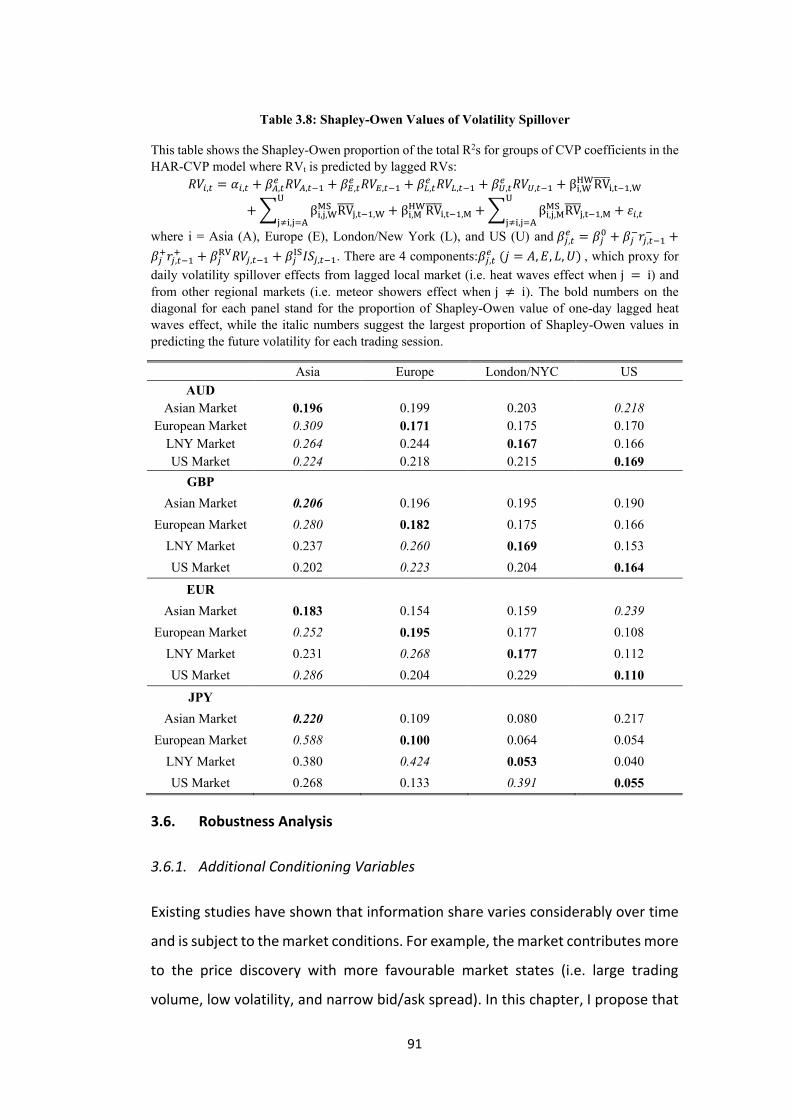
91

Table 3.8: Shapley-Owen Values of Volatility Spillover

This table shows the Shapley-Owen proportion of the total R2s for groups of CVP coefficients in the

HAR-CVP model where RVt is predicted by lagged RVs:




i,t−1,W


j,t−1,W

U

j≠i,j=A+ βi,M



U



0 + 𝛽𝑗−𝑟𝑗,𝑡−1

− +



IS𝐼𝑆𝑗,𝑡−1. There are 4 components:𝛽𝑗,𝑡𝑒 (𝑗 = 𝐴, 𝐸, 𝐿, 𝑈) , which proxy for

daily volatility spillover effects from lagged local market (i.e. heat waves effect when j = i) and

from other regional markets (i.e. meteor showers effect when j ≠ i). The bold numbers on the

diagonal for each panel stand for the proportion of Shapley-Owen value of one-day lagged heat

waves effect, while the italic numbers suggest the largest proportion of Shapley-Owen values in

predicting the future volatility for each trading session.


AUD

Asian Market 0.196 0.199 0.203 0.218

European Market 0.309 0.171 0.175 0.170

LNY Market 0.264 0.244 0.167 0.166

US Market 0.224 0.218 0.215 0.169

GBP

Asian Market 0.206 0.196 0.195 0.190

European Market 0.280 0.182 0.175 0.166

LNY Market 0.237 0.260 0.169 0.153

US Market 0.202 0.223 0.204 0.164

EUR

Asian Market 0.183 0.154 0.159 0.239

European Market 0.252 0.195 0.177 0.108

LNY Market 0.231 0.268 0.177 0.112

US Market 0.286 0.204 0.229 0.110

JPY

Asian Market 0.220 0.109 0.080 0.217

European Market 0.588 0.100 0.064 0.054

LNY Market 0.380 0.424 0.053 0.040

US Market 0.268 0.133 0.391 0.055

3.6. Robustness Analysis

3.6.1. Additional Conditioning Variables

Existing studies have shown that information share varies considerably over time

and is subject to the market conditions. For example, the market contributes more

to the price discovery with more favourable market states (i.e. large trading

volume, low volatility, and narrow bid/ask spread). In this chapter, I propose that

92

volatility persistence is driven by the characteristics of both exogenous and

endogenous information arrivals and strategic trading such as portfolio

adjustments to lagged information shocks. Collectively these mechanisms

determine the state of the market, and in turn, impact volatility persistence. The

use of market state variables (i.e., number of trades, illiquidity, and order

imbalance) as the additional conditioning variables is in the same spirit as Wang

and Yang (2017) who examine whether daily volatility persistence is affected by

volatility jumps (VJ), number of trades (NT), illiquidity (IL), and the imbalance of

buyer- and seller-initiated trades (TI) in the stock market. Namely, the market

state variables include return, trading volume, illiquidity, order imbalance, and

volatility (see, Brandt et al., 2007; Mizrach and Neely, 2008; Frijns, Lehnert and

Zwinkels, 2010; Su and Zhang, 2018).

The market state variables for each segment are constructed as follows: trading

volume is defined as the number of trades aggregated over 5-minute intervals;

daily illiquidity is measured by the Amihud (2002)’s illiquidity measure, which is

defined as 𝐼𝐿𝑡 = |𝑟𝑡|/𝑁𝑇𝑡 where 𝑁𝑇𝑡 is the number of trades and |𝑟𝑡| is the

absolute value of return over 5-minute intervals. For the order imbalance,

following Wang and Yang (2017), I use the method of “bulk volume” classification

(BVC) of Easley, de Prado and O’Hara (2012) to partition the number of trades into

buyer- and seller-initiated portions sampled at 5-minute intervals. Then the

difference between these two portions is termed the order imbalance ( 𝑂𝐼𝑡 ).

Recently, Chakrabarty, Pascual, and Shkilko (2015) prove that BVC is better linked

to proxies of information-based trading, compared to Lee and Ready (1991)’s

trade classification algorithm.

The summary statistics of market state variables (including return, volatility,

information share, number of trade, illiquidity, and order imbalance) by trading

sessions are reported in Appendix G. As shown in Panel A of Appendix G, AUD/USD

has the highest volatility during the Asian market, while the lowest volatility in LNY

market. The returns in the four markets have the same direction of skewness, i.e.

the distributions of returns are left skewed, or negatively skewed. The Ljung-Box

93

statistics show that the returns have weak autocorrelations at 5 lags in the Asian

and North American markets, while there is little or no autocorrelation in

European market. The transactions concentrate in the Europe and LNY markets,

particularly for GBP and EUR. Besides, the order imbalances are not statistically

different from zero in all trading sessions, which confirms earlier works on FX

microstructure suggesting that dealers generally tend to “hold positions for very

short time horizons, typically under a day, and have zero inventory overnight”

(King et al., 2011). Appendix G also presents the summary statistics of the daily

information shares measured as the TSRV ratio in four trading sessions, among

which Europe has the largest estimated information share, followed by the U.S.,

Asia, and “LNY” market. The information share of Asia has the largest standard

deviation, while the strongest autocorrelations at lag 12. Besides, the information

shares in four markets are negatively correlated, suggesting increased information

shares of one trading session is associated with decreased information shares for

other sessions.

This section presents a robustness analysis where volatility spillovers (namely,

meteor showers and heat waves effects) are regressed on exchange rate returns,

volatility, and other additional variables. Namely, in addition to daily return and

RV, I examine whether daily volatility spillovers are affected by other conditioning

variables, including Amihud’s illiquidity measure (IL), number of trades (NT), and

order imbalance (OI). Let Yt-1 be one of these variables on day t-1. To assess the

impacts of these variables on volatility persistence, I extend the model in Eq. (5.1)

to include Yt-1 and its interaction with RVt. However, I don’t find any consistent

effects of the additional market state variables in explaining the conditional

volatility persistence.33 Besides, I also attempt to examine the impacts of investors’

sensitivity to information on volatility persistence as documented in Berger et al.

(2009), however, these effects are insignificant under most circumstances. One of

the possible reasons is that I focus on the lead-lag effects rather than the

contemporaneous relationships as documented in the earlier literature. Overall,

33 The results of additional conditioning variables are not presented here for the sake of brevity, however, which are available upon request.

94

these empirical findings are consistent with those of Wang and Yang (2017) who

examine the volatility persistence in the equity markets and find no effects of the

additional market state variables. The results are also consistent with those of

Gillemot, Farmer, and Lillo (2006), who conclude that “the long-memory of

volatility is dominated by factors other than transaction frequency or total trading

volume”.

3.6.2. Out-of-sample forecasting performance

In this robustness analysis sub-section, I compare the ex-post out-of-sample

forecasting performances of various volatility models. Namely, if the daily volatility

persistence varies as a function of the observed market condition, the model

which calibrates RV dynamics conditional on market state variables should provide

superior forecast performance. To examine the forecasting performances, I first

estimate the model parameters using the first 5 years of observations as the in-

sample period, and then use the rest of the sample as the out-of-sample period.

All forecasts are generated using rolling WLS regressions and parameter estimates

are updated daily. Forecasting performance is evaluated based on two loss

functions: the negative quasi-likelihood function QLIKE(RV𝑡 , RV̂𝑡) =RV𝑡

RV̂𝑡−

ln (RV𝑡

RV̂𝑡) − 1 and the logarithmic mean-squared errors LMSE(RV𝑡 , RV̂𝑡) =

(ln(RV𝑡) − ln (RV̂𝑡))2 , where RV̂𝑡 is the forecasted value of RV𝑡 . Patton (2012)

shows that QLIKE is robust to the noise in the empirical volatility measures. Patton

and Sheppard (2009) show that QLIKE has the best size-adjusted power among

robust loss functions. The usual mean-squared error (MSE) is often affected by a

few extreme observations. Therefore, I use the logarithmic MSE to mitigate this

problem. Furthermore, forecast performance is examined by the Diebold-Mariano

(1995)’s test (i.e., DM statistics). Specifically, taking the HAR model as the

benchmark, a negative DM statistic indicates a reduction in loss value by other

volatility models relative to HAR. While HAR is nested in CVP model, Giacomini and

White (2006) show that the DM test remains asymptotically valid when the

estimation period is finite.

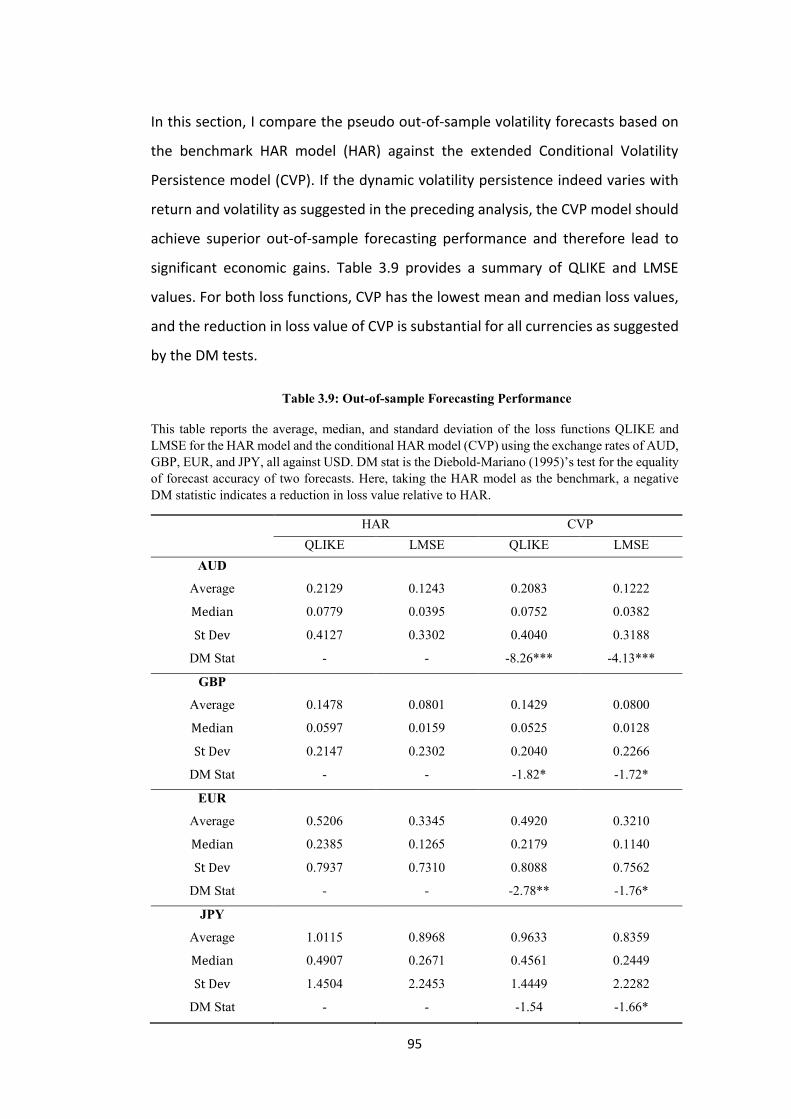
95

In this section, I compare the pseudo out-of-sample volatility forecasts based on

the benchmark HAR model (HAR) against the extended Conditional Volatility

Persistence model (CVP). If the dynamic volatility persistence indeed varies with

return and volatility as suggested in the preceding analysis, the CVP model should

achieve superior out-of-sample forecasting performance and therefore lead to

significant economic gains. Table 3.9 provides a summary of QLIKE and LMSE

values. For both loss functions, CVP has the lowest mean and median loss values,

and the reduction in loss value of CVP is substantial for all currencies as suggested

by the DM tests.

Table 3.9: Out-of-sample Forecasting Performance

This table reports the average, median, and standard deviation of the loss functions QLIKE and

LMSE for the HAR model and the conditional HAR model (CVP) using the exchange rates of AUD,

GBP, EUR, and JPY, all against USD. DM stat is the Diebold-Mariano (1995)’s test for the equality

of forecast accuracy of two forecasts. Here, taking the HAR model as the benchmark, a negative

DM statistic indicates a reduction in loss value relative to HAR.

HAR CVP

QLIKE LMSE QLIKE LMSE

AUD

Average 0.2129 0.1243 0.2083 0.1222

Median 0.0779 0.0395 0.0752 0.0382

St Dev 0.4127 0.3302 0.4040 0.3188

DM Stat - - -8.26*** -4.13***

GBP

Average 0.1478 0.0801 0.1429 0.0800

Median 0.0597 0.0159 0.0525 0.0128

St Dev 0.2147 0.2302 0.2040 0.2266

DM Stat - - -1.82* -1.72*

EUR

Average 0.5206 0.3345 0.4920 0.3210

Median 0.2385 0.1265 0.2179 0.1140

St Dev 0.7937 0.7310 0.8088 0.7562

DM Stat - - -2.78** -1.76*

JPY

Average 1.0115 0.8968 0.9633 0.8359

Median 0.4907 0.2671 0.4561 0.2449

St Dev 1.4504 2.2453 1.4449 2.2282

DM Stat - - -1.54 -1.66*

96

3.7. Conclusions and Implications

In this chapter, I revisit the meteor shower and heat wave effects for AUD/USD,

GBP/USD, EUR/USD, and USD/JPY spanning from January 1999 (January 2000 for

EUR) to December 2013. Utilizing the volatility measures based on high-frequency

data, I find evidence of both meteor showers and heat waves effects in the four

trading segments of global FX market, which is consistent with Lahaye and Neely

(2016) who divide a calendar day into five segments and confirm the presence of

meteor shower and heat waves effect in each segment. However, unlike Lahaye

and Neely (2016), I find that the relative importance of meteor shower effect has

been increasing rapidly and has predominated over heat waves effects in the intra-

daily volatility spillovers, which emphasizes the increasing interdependence and

interconnectedness in the global FX market, and highlights the potential contagion

risks posed by financial liberalization and market openness.

By investigating the pattern and economic mechanism of meteor showers and

heat waves effects, I contribute to the literature regarding volatility spillover in the

financial markets. Specifically, I identify the key factors contributing to volatility

spillovers in different trading sessions of the FX market. The empirical results also

highlight the complex geographical nature of the FX market. That is, the spillover

effect of volatility depends on where the information shocks arise. This study has

modelling implications for the FX market as well. For example, these results argue

in favour of modelling FX volatility dynamics segment-wise, rather than in the

more traditional approach of assuming a homogeneous process.

In this study, I also contribute to the growing literature on information

propagation in the foreign exchange market. By exploring the economic

mechanism of volatility spillover in the exchange rates, the findings presented in

this study highlight the impacts of changing market states on the volatility

spillovers, which could be the results of exogeneous and endogenous information

arrivals, the persistence of characteristics of information propagation process, and

uninformed trading in response to lagged information shocks, etc. The analysis in

this chapter builds upon ideas contained in the literature on mixture of

97

distributions hypothesis (MDH) (Liesenfeld, 2001). However, this particular

volatility model is based on relationships introduced in the market microstructure

literature, and the estimation relies on the availability of a long time-series of

trading data at very high frequency. Besides, different from the conventional MDH,

I find that volatility spillover is not solely determined by exogenous information

arrivals, but also by the process of absorbing information shocks and resolving

uncertainty. Namely, a faster process of price discovery within a period reduces

information persistence to future periods and mitigates volatility spillover to other

markets.

However, additional research is required to consider how generalizable the results

presented in this chapter are to other major currencies and emerging market

currencies. Besides, how to identify the institutional sources of long-memory in

volatility (i.e. institution- and market-wide characteristics) deserves further study,

which will definitely improve the understanding of volatility spillover and extend

our economic intuition of risk contagion in the financial markets. Also, if there is a

common component in conditional volatility, should provide more evidence on

the factors driving the variations in exchange rate returns. Another possible

direction is to assess the usefulness and economic values of conditional volatility

persistence in concrete financial applications such as portfolio management and

volatility timing strategy as in Fleming et al. (2003).

98

Chapter 4: Conditional Volatility Persistence and Volatility Timing in

the Foreign Exchange Market

4.1. Introduction

The phenomenon of volatility, i.e., up-and-down movements of the market, plays

a central role in derivatives pricing, risk management, and optimal portfolio. It

draws great attention to academics, practitioners, and regulators, and motivates

a vast amount of literature on volatility modelling. Starting from Engle (1982), a

variety of autoregressive conditional heteroskedasticity (ARCH), generalized ARCH

(GARCH), and stochastic volatility (SV) models have been fit to asset returns.

However, starting with Andersen and Bollerslev (1998) and Andersen et al. (2003),

the literature has been increasingly focused on so-called realized volatility (RV)

models with the availability of quality high-frequency data (see, for example,

Bollerslev, Chou and Kroner, 1992; Bollerslev, Engle and Nelson, 1994; Diebold and

Lopez, 1995; and recently, Bollerslev et al., 2017). The empirical evidence on

volatility is generally consistent across a wide range of assets and econometric

specifications, which overwhelmingly suggests that volatility is predictable to a

great extent. These literature, however, has been exclusively focused on

evaluating the statistical performance of volatility models rather than the

economic significance of predictive volatility. Following Fleming, Kirby, and

Ostdiek (2001, 2003) and Bollerslev et al. (2017), I focus on the latter. Namely, I

not only conduct an extensive statistical evaluation of volatility forecasting using

a variant of heterogeneous autoregressive (HAR) models, but also provide new

economic evidence on whether a risk-averse investor can significantly benefit

from volatility-timing based on mean-variance analysis. Furthermore, I explore the

economic mechanisms of the conditional volatility persistence, which help in

achieving superior forecasting performance and potential economic gains.

Volatility persistence is a well-documented phenomenon across a broad range of

financial markets, including the Foreign Exchange market. This suggests that

standard volatility models deliver reasonably accurate forecasts, but the question

99

of whether volatility timing has economic value still remains unanswered,

particularly when forecasting using the model which incorporates the features of

volatility asymmetry and persistence. In short, the economic value of volatility

timing is the utility gain compared with a static strategy. For an investor with a

mean-variance utility, the major concern is to estimate the fee she is willing to pay

for a new volatility model rather than a static one. In this chapter, I apply the

conditional volatility persistence model as proposed in Wang and Yang (2017) to

the FX market, and examine the presence of volatility persistence in the exchange

rates and its determinants by taking a much broader view on the economic

mechanisms of the volatility persistence. In addition, I adopt an optimal

rebalancing strategy in volatility targeting solutions and utilize the technique of

backtesting to examine the ex-post performance of optimal portfolio holdings.

This approach has several advantages over existing studies. First, instead of

measuring the benefits of predictability via ex-ante calibration (Balduzzi and Lynch,

1999; Campbell and Viceira, 1999; and Campbell, Chan and Viceira, 2002), I

measure economic benefits through the ex-post performance of the optimal

portfolio with predictable volatility. More importantly, considering that there is

little evidence for any out-of-sample expected return predictability (Bossaerts and

Hillion, 1999), I focus exclusively on the prediction of realized variance, which

eliminates the noise form random return realizations and provides a practical

evaluation of the economic benefits. Second, ignoring estimation risk or

parameter learning (i.e., the dynamic counterpart of estimation risk) that arises

when estimating parameters would typically lead to misleading allocations

(Brennan, 1998; Stambaugh, 1999; Barberis, 2000). By utilizing a non-parametric

“realized utility” technique as proposed in Bollerslev et al. (2017), I solve the

single-period asset allocation problem while accounting for estimation risk and

parameter learning, since “the multi-period portfolio problem with time-varying

expected returns or volatility in the presence of estimation risk or parameter

learning is computationally intractable” (Johannes et al. 2002). The main

difference between the single- and multi-period asset allocation problems is

intertemporal hedging demands. However, recent evidence suggests that ignoring

100

hedging demands would not be a major concern, since they are typically only a

small component of asset demands (see Brandt, 1999; Ait-Sahalia and Brandt,

2001).

This chapter contributes to the extant literature on the economic value of volatility

timing in several different ways. Firstly, previous studies demonstrate that

volatility timing strategy can be enhanced by using high frequency data, optimal

sampling, optimal rebalancing frequencies, and noise- and jump-robust volatility

measures (See, for example, Fleming et al., 2001, 2003; Bandi and Russell, 2006;

Bandi, Russell, and Zhu, 2008; Nolte and Xu, 2015). I extend the previous studies

by considering the economic value of conditional volatility persistence model,

which explicitly links the changing overall market conditions to the future volatility

and far surpasses the benchmark models with regard to the forecasting

performance. Besides, although more sophisticated utility functions can be

utilized, I stick to a simple mean-variance utility because the major concern is to

examine whether statistical improvements in volatility forecasting by taking the

time-varying volatility persistence into consideration can be translated into

economic gains. Furthermore, to concentrate on the impacts of volatility timing, I

assume only one risky asset in each portfolio to avoid covariance matrix

forecasting in a multivariate setting and control for information spillover across

different assets. I also assume that the investor is myopic, and she does not

consider the hedging demand when constructing the optimal portfolio. I make this

assumption for both simplicity and consistency. Namely, without loss of generality,

the volatility forecasting results generated can be easily translated into certainty

equivalent performance fees and directly compared with those documented in the

existing literature on the economic value of volatility timing. In summary, I

conclude the main findings as follows:

(1) Utilizing the conditional volatility persistence (CVP) model as proposed in

Wang and Yang (2017), I find that the conditional volatility persistence increases

with information shocks as proxied by negative and positive returns, while

decreases with information flows as proxied by realized variance. Taking into

101

account conditional volatility persistence improves volatility forecasting

performance both in-sample and out-of-sample. For example, by utilizing the

Shapley decomposition techniques, I find that the conditional volatility persistence

explains large portions of the variations in future volatility and is the dominant

channel linking changing market conditions to future volatility. However, I provide

mixed evidence on asymmetric effects in the FX market, to which similar results

have been found in Wang and Yang (2009).

(2) Under conservative assumptions about the Sharpe ratio and the investor’s

risk aversion, having a Heterogeneous Autoregressive (HAR) - based model which

takes the conditional volatility persistence into consideration is worth about 0.51%

of total wealth per year relative to the static risk model (i.e., using in-sample

average volatility). And the utility gains are even larger during the crisis period or

under the assumption of higher Sharpe ratio and/or lower risk aversion. Besides,

the gains in using the conditional volatility persistence model remain positive and

significant after accounting for transaction costs and market microstructure noise.

(3) The volatility targeting approach which utilizes dynamic asset allocation

based on accurate volatility forecasting can take advantage of the negative

relationship between volatility and return and the properties of volatility

persistence, and achieves a stable level of volatility in all market environments.

The economic gains of volatility targeting are significant (i.e., the Sharpe ratio of

volatility timing strategy using CVP model is as high as 1.23, compared to 0.83 for

that without volatility timing).

The rest of this chapter is structured as follows. Section 4.2 introduces the data

and construction of relevant variables. Section 4.3 presents the model

specifications including the classic Heterogeneous Autoregressive model (HAR),

the semi-variance Heterogeneous Autoregressive model (SHAR), and the

Conditional Volatility Persistence model (CVP). A simple utility-based framework

for quantifying the economic gains of the new risk models is given in this section

as well. Section 4.4 compares the forecasting performances of various risk models

and discusses the utility benefits under different scenarios. Section 4.5 performs a

robustness check, while Section 4.6 concludes with further research directions.

102

4.2. Variable Construction and Summary Statistics

4.2.1. Data Description

The data source is Thomson Reuters Tick History (TRTH) supplied by the Securities

Industry Research Centre of Asia-Pacific (SIRCA). The intraday data for AUD/USD,

GBP/USD and USD/JPY spans from 1 January 1999 to 31 December 2013, while the

data for EUR/USD isn’t available until 1 January 2000. The four currencies I am

using in this chapter are among top-5 most actively traded currencies and account

for more than 50% of the globe FX trading (Bank for International Settlements,

2013). The dataset includes the time rounded to the nearest millisecond whenever

a new quote is posted, prices of firm bid/ask quotes, trading time, and trading

prices. Following other studies such as Bollerslev and Domowitz (1993), I exclude

weekends, because of thin and inconsistent trading. I define weekends as

extending from 22:00 GMT Friday evening (i.e., the end of day trading session in

New York) until 22:00 GMT Sunday evening (i.e., the commencement of morning

trading session in Sydney). In consistent with Wang and Yang (2011), I remove days

with large time gaps (i.e. over four hours) in quote arrivals, which could be the

result of holidays in major financial centres, system halts, or other technical issues.

I also exclude observations which deviate by more than 10 times standard

deviations from a rolling sample of 50 observations. Last but not least, to mitigate

the potential impacts of extremely large values, I winsorize the daily realized

variance at the 99th percentile.

4.2.2. Integrated Variance

In recent years, there has been a renewed interest in obtaining improved daily

volatility estimates by constructing daily “realized” or “integrated” volatility with

the availability of quality high-frequency data (Thomakos and Wang, 2010). The

most popular estimator is realized volatility, see Andersen et al. (2003) for a review.

Namely, daily realized volatility can be obtained as the sum of intraday squared

returns. Using the theory of quadratic variation, Andersen and Bollerslev (1998)

and Barndorff-Nielsen and Shephard (2002) show that the realized volatility

estimator is a model-free estimator of the true but latent volatility.

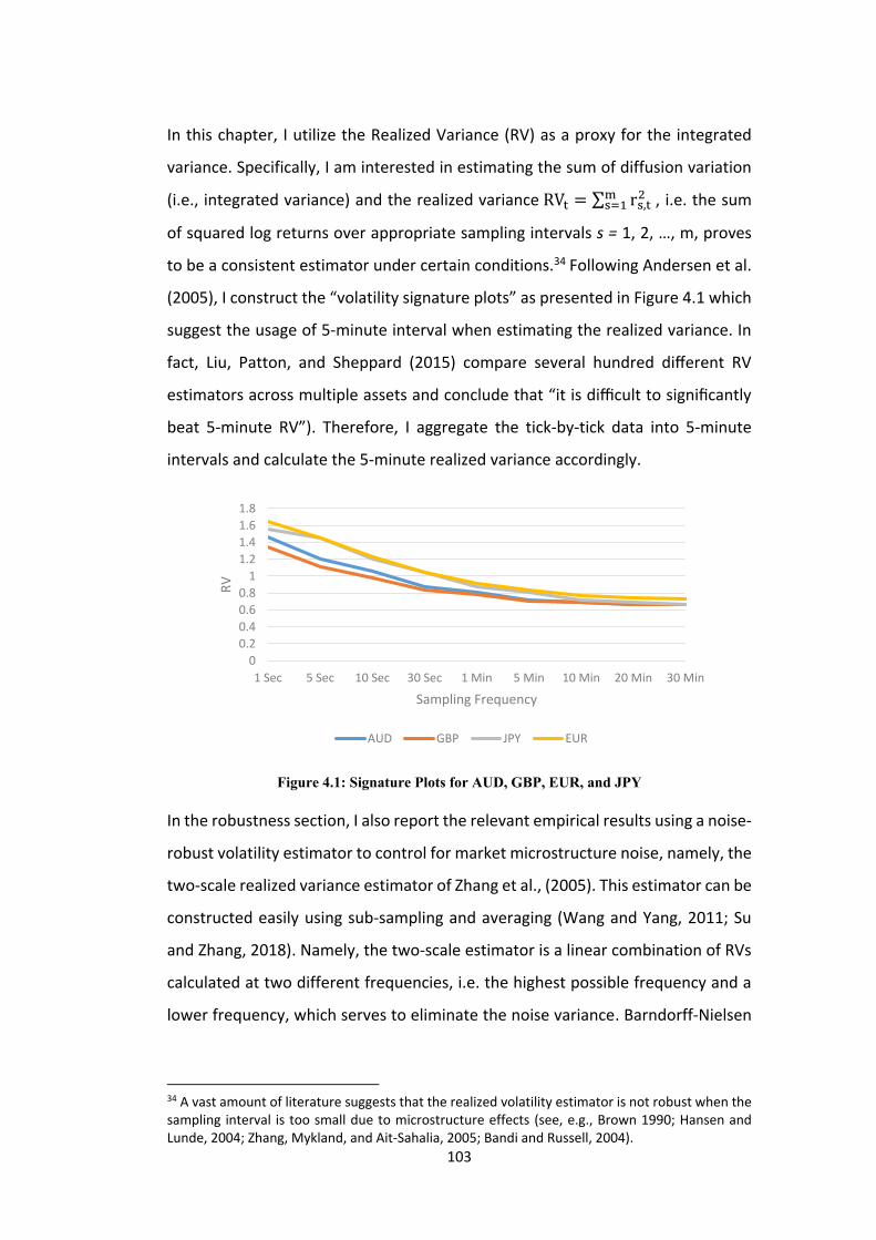
103

In this chapter, I utilize the Realized Variance (RV) as a proxy for the integrated

variance. Specifically, I am interested in estimating the sum of diffusion variation

(i.e., integrated variance) and the realized variance RVt = ∑ rs,t2m

s=1 , i.e. the sum

of squared log returns over appropriate sampling intervals s = 1, 2, …, m, proves

to be a consistent estimator under certain conditions.34 Following Andersen et al.

(2005), I construct the “volatility signature plots” as presented in Figure 4.1 which

suggest the usage of 5-minute interval when estimating the realized variance. In

fact, Liu, Patton, and Sheppard (2015) compare several hundred different RV

estimators across multiple assets and conclude that “it is difficult to significantly

beat 5-minute RV”). Therefore, I aggregate the tick-by-tick data into 5-minute

intervals and calculate the 5-minute realized variance accordingly.

Figure 4.1: Signature Plots for AUD, GBP, EUR, and JPY

In the robustness section, I also report the relevant empirical results using a noise-

robust volatility estimator to control for market microstructure noise, namely, the

two-scale realized variance estimator of Zhang et al., (2005). This estimator can be

constructed easily using sub-sampling and averaging (Wang and Yang, 2011; Su

and Zhang, 2018). Namely, the two-scale estimator is a linear combination of RVs

calculated at two different frequencies, i.e. the highest possible frequency and a

lower frequency, which serves to eliminate the noise variance. Barndorff-Nielsen

34 A vast amount of literature suggests that the realized volatility estimator is not robust when the sampling interval is too small due to microstructure effects (see, e.g., Brown 1990; Hansen and Lunde, 2004; Zhang, Mykland, and Ait-Sahalia, 2005; Bandi and Russell, 2004).

0

0.2

0.4

0.6

0.8

1

1.2

1.4

1.6

1.8

1 Sec 5 Sec 10 Sec 30 Sec 1 Min 5 Min 10 Min 20 Min 30 Min

RV

Sampling Frequency

AUD GBP JPY EUR

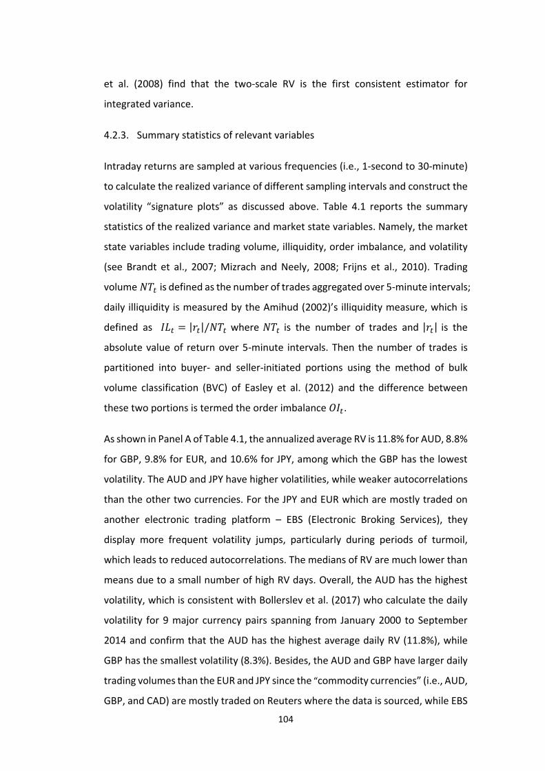
104

et al. (2008) find that the two-scale RV is the first consistent estimator for

integrated variance.

4.2.3. Summary statistics of relevant variables

Intraday returns are sampled at various frequencies (i.e., 1-second to 30-minute)

to calculate the realized variance of different sampling intervals and construct the

volatility “signature plots” as discussed above. Table 4.1 reports the summary

statistics of the realized variance and market state variables. Namely, the market

state variables include trading volume, illiquidity, order imbalance, and volatility

(see Brandt et al., 2007; Mizrach and Neely, 2008; Frijns et al., 2010). Trading

volume 𝑁𝑇𝑡 is defined as the number of trades aggregated over 5-minute intervals;

daily illiquidity is measured by the Amihud (2002)’s illiquidity measure, which is

defined as 𝐼𝐿𝑡 = |𝑟𝑡|/𝑁𝑇𝑡 where 𝑁𝑇𝑡 is the number of trades and |𝑟𝑡| is the

absolute value of return over 5-minute intervals. Then the number of trades is

partitioned into buyer- and seller-initiated portions using the method of bulk

volume classification (BVC) of Easley et al. (2012) and the difference between

these two portions is termed the order imbalance 𝑂𝐼𝑡.

As shown in Panel A of Table 4.1, the annualized average RV is 11.8% for AUD, 8.8%

for GBP, 9.8% for EUR, and 10.6% for JPY, among which the GBP has the lowest

volatility. The AUD and JPY have higher volatilities, while weaker autocorrelations

than the other two currencies. For the JPY and EUR which are mostly traded on

another electronic trading platform – EBS (Electronic Broking Services), they

display more frequent volatility jumps, particularly during periods of turmoil,

which leads to reduced autocorrelations. The medians of RV are much lower than

means due to a small number of high RV days. Overall, the AUD has the highest

volatility, which is consistent with Bollerslev et al. (2017) who calculate the daily

volatility for 9 major currency pairs spanning from January 2000 to September

2014 and confirm that the AUD has the highest average daily RV (11.8%), while

GBP has the smallest volatility (8.3%). Besides, the AUD and GBP have larger daily

trading volumes than the EUR and JPY since the “commodity currencies” (i.e., AUD,

GBP, and CAD) are mostly traded on Reuters where the data is sourced, while EBS

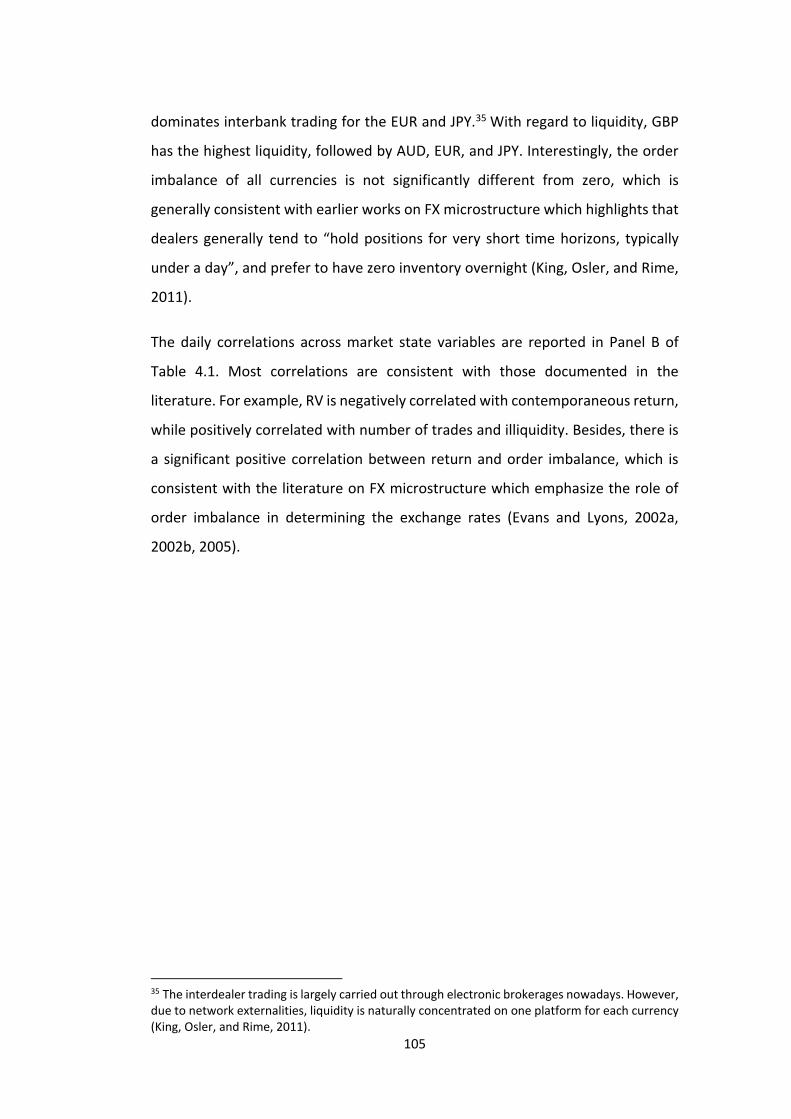
105

dominates interbank trading for the EUR and JPY.35 With regard to liquidity, GBP

has the highest liquidity, followed by AUD, EUR, and JPY. Interestingly, the order

imbalance of all currencies is not significantly different from zero, which is

generally consistent with earlier works on FX microstructure which highlights that

dealers generally tend to “hold positions for very short time horizons, typically

under a day”, and prefer to have zero inventory overnight (King, Osler, and Rime,

2011).

The daily correlations across market state variables are reported in Panel B of

Table 4.1. Most correlations are consistent with those documented in the

literature. For example, RV is negatively correlated with contemporaneous return,

while positively correlated with number of trades and illiquidity. Besides, there is

a significant positive correlation between return and order imbalance, which is

consistent with the literature on FX microstructure which emphasize the role of

order imbalance in determining the exchange rates (Evans and Lyons, 2002a,

2002b, 2005).

35 The interdealer trading is largely carried out through electronic brokerages nowadays. However, due to network externalities, liquidity is naturally concentrated on one platform for each currency (King, Osler, and Rime, 2011).

106

Table 4.1: Summary Statistics

This table reports the summary statistics of market state variables. IL, NT, and OI stand for illiquidity,

number of trades, and order imbalance respectively. QLB(5) is the Ljung-Box test statistic at 5 lags.

The numbers in the square brackets are the corresponding P-values. The asterisks ***, **, * indicate

that the values are statistically different from zero at 1%, 5%, and 10% respectively.

Panel A: Summary statistics of market state variables

Mean Median St Dev Skew Kurt Min Max QLB(5)

AUD

Return .0002 .0003 .0082 -.3572 7.213 -.0733 .0737 24.39*

RV .7076 .4648 .8265 4.001 19.48 .1063 5.946 9,800*

IL 2.995 2.534 .1.279 1.016 .7014 1.191 9.767 16,216*

NT 8.441 5.994 6.746 1.183 1.509 .0540 48.86 9,358*

OI -.0330 -.0077 .3782 -.5142 5.483 -2.334 2.091 53.49*

GBP

Return .0002 .0002 .0057 -.2158 2.190 -.0350 .0299 2.461

RV .3683 .2658 .3635 3.535 14.51 .0666 2.428 11,364*

IL 1.936 1.820 .6356 2.031 7.235 .8892 6.887 13,404*

NT 7.120 6.693 3.405 .5934 .1704 .0330 26.82 9,155*

OI -.0200 -.0100 .3516 -.2010 2.462 -2.217 1.785 10.05

EUR

Return .0002 .0002 .0065 .4678 5.938 -.0305 .0693 2.214

RV .9537 .4900 1.486 4.493 24.41 .0793 11.23 5,029*

IL 4.247 3.307 2.651 1.794 4.018 1.255 18.22 11,505*

NT 1.703 1.583 .9124 .6024 .0886 .0010 5.864 4,067*

OI .0090 .0010 .1334 .2987 1.505 -.5160 .8520 21.11*

JPY

Return -.0001 .0000 .0066 -.3655 4.132 -.0488 .0365 3.888

RV 1.346 .5892 2.486 4.561 23.84 .0522 17.85 2,259*

IL 8.108 7.681 3.500 .4655 -.4295 1.899 23.19 8,870*

NT .1720 .1410 .1291 2.104 9.002 .0000 1.657 1,833*

OI -.0020 -.0010 .0013 -2.102 9.018 -.6570 .7770 6.44

107

Panel B: Correlations

4.3. Model Specification

4.3.1. HAR Model

In this chapter, I employ variants of the heterogeneous autoregressive (HAR)

models, which takes into account the heterogeneous impacts of investors at

different trading horizons (i.e., daily, weekly, and monthly horizon respectively),

while capturing the property of long-memory in volatility. The HAR model was

firstly proposed in Corsi (2009), which is based on the concept of the

Heterogeneous Market Hypothesis of Muller et al. (1997), and has been employed

in several applications, such as for equity markets (Andersen, Bollerslev, and

Return RV NT OI IL

AUD

RV -.0667***

[.0000] 1.000

NT -.0671***

[.0000]

.2838***

[.0000] 1.000

OI .7083***

[.0000]

-.0703***

[.0000]

-.1643***

[.0000] 1.000

IL -.0522***

[.0013]

.4703***

[.0000]

-.3453***

[.0000]

.0088

[.5894] 1.000

GBP

RV -.0442***

[.0061] 1.000

NT -.0180

[.2674]

.4105***

[.0000] 1.000

OI .8071***

[.0000]

-.0354**

[.0285]

-.0419***

[.0094] 1.000

IL -.0212

[.1887]

.5306***

[.0000]

-.1773***

[.0000]

-.0077

[.6358] 1.000

EUR

RV -.0419*

[.1004] 1.000

NT .0184

[.2871]

.0914***

[.0000] 1.000

OI .5733***

[.0000]

.0046

[.5861]

.0546***

[.0014] 1.000

IL -.0230

[.1459]

.6144***

[.0000]

-.1737***

[.0000]

.0006

[.9743] 1.000

JPY

RV -.0621***

[.0009] 1.000

NT -.0119

[.5219]

.1465***

[.0000] 1.000

OI .7719

[.0000]

.0012

[.9122]

-.0012

[.1221] 1.000

IL -.0432**

[.0204]

.5598***

[.0000]

-.1064*

[.0716]

.0002

[.9879] 1.000

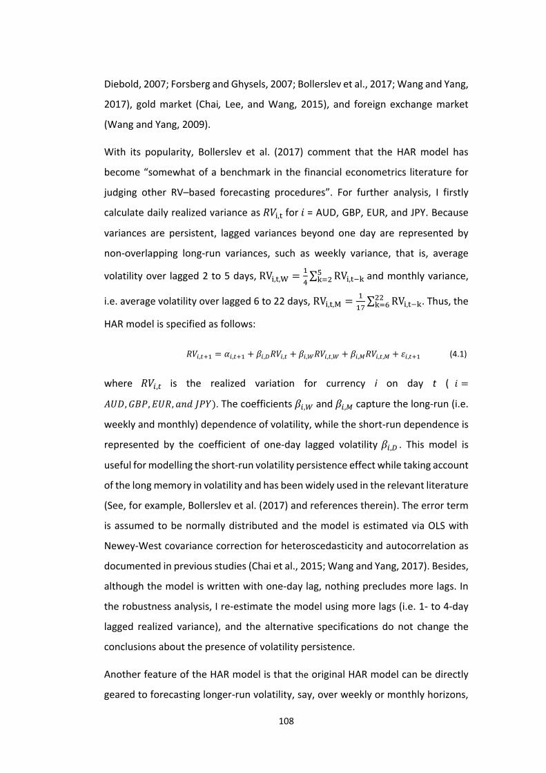
108

Diebold, 2007; Forsberg and Ghysels, 2007; Bollerslev et al., 2017; Wang and Yang,

2017), gold market (Chai, Lee, and Wang, 2015), and foreign exchange market

(Wang and Yang, 2009).

With its popularity, Bollerslev et al. (2017) comment that the HAR model has

become “somewhat of a benchmark in the financial econometrics literature for

judging other RV–based forecasting procedures”. For further analysis, I firstly

calculate daily realized variance as 𝑅𝑉i,t for 𝑖 = AUD, GBP, EUR, and JPY. Because

variances are persistent, lagged variances beyond one day are represented by

non-overlapping long-run variances, such as weekly variance, that is, average

volatility over lagged 2 to 5 days, RVi,t,W =1

4∑ RVi,t−k

5k=2 and monthly variance,

i.e. average volatility over lagged 6 to 22 days, RVi,t,M =1

17∑ RVi,t−k

22k=6 . Thus, the

HAR model is specified as follows:

𝑅𝑉𝑖,𝑡+1 = 𝛼𝑖,𝑡+1 + 𝛽𝑖,𝐷𝑅𝑉𝑖,𝑡 + 𝛽𝑖,𝑊𝑅𝑉𝑖,𝑡,𝑊 + 𝛽𝑖,𝑀𝑅𝑉𝑖,𝑡,𝑀 + 𝜀𝑖,𝑡+1 (4.1)

where 𝑅𝑉𝑖,𝑡 is the realized variation for currency i on day t ( 𝑖 =

𝐴𝑈𝐷, 𝐺𝐵𝑃, 𝐸𝑈𝑅, 𝑎𝑛𝑑 𝐽𝑃𝑌). The coefficients 𝛽𝑖,𝑊 and 𝛽𝑖,𝑀 capture the long-run (i.e.

weekly and monthly) dependence of volatility, while the short-run dependence is

represented by the coefficient of one-day lagged volatility 𝛽𝑖,𝐷 . This model is

useful for modelling the short-run volatility persistence effect while taking account

of the long memory in volatility and has been widely used in the relevant literature

(See, for example, Bollerslev et al. (2017) and references therein). The error term

is assumed to be normally distributed and the model is estimated via OLS with

Newey-West covariance correction for heteroscedasticity and autocorrelation as

documented in previous studies (Chai et al., 2015; Wang and Yang, 2017). Besides,

although the model is written with one-day lag, nothing precludes more lags. In

the robustness analysis, I re-estimate the model using more lags (i.e. 1- to 4-day

lagged realized variance), and the alternative specifications do not change the

conclusions about the presence of volatility persistence.

Another feature of the HAR model is that the original HAR model can be directly

geared to forecasting longer-run volatility, say, over weekly or monthly horizons,

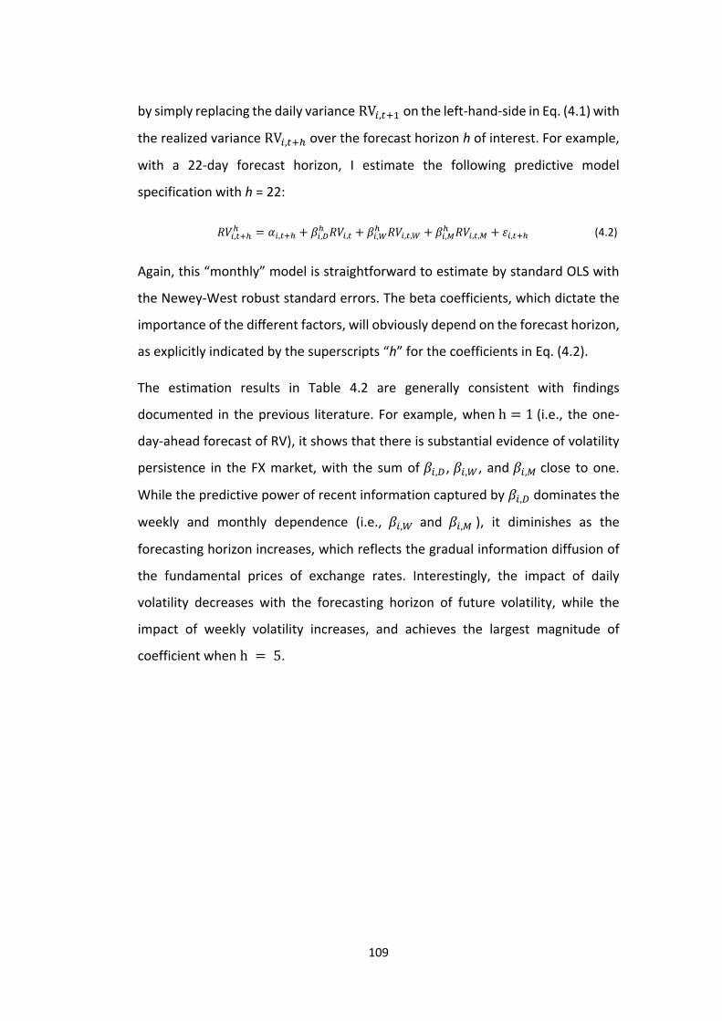
109

by simply replacing the daily variance RV𝑖,𝑡+1 on the left-hand-side in Eq. (4.1) with

the realized variance RV𝑖,𝑡+ℎ over the forecast horizon h of interest. For example,

with a 22-day forecast horizon, I estimate the following predictive model

specification with h = 22:

𝑅𝑉𝑖,𝑡+ℎℎ = 𝛼𝑖,𝑡+ℎ + 𝛽𝑖,𝐷

ℎ 𝑅𝑉𝑖,𝑡 + 𝛽𝑖,𝑊ℎ 𝑅𝑉𝑖,𝑡,𝑊 + 𝛽𝑖,𝑀

ℎ 𝑅𝑉𝑖,𝑡,𝑀 + 𝜀𝑖,𝑡+ℎ (4.2)

Again, this “monthly” model is straightforward to estimate by standard OLS with

the Newey-West robust standard errors. The beta coefficients, which dictate the

importance of the different factors, will obviously depend on the forecast horizon,

as explicitly indicated by the superscripts “h” for the coefficients in Eq. (4.2).

The estimation results in Table 4.2 are generally consistent with findings

documented in the previous literature. For example, when h = 1 (i.e., the one-

day-ahead forecast of RV), it shows that there is substantial evidence of volatility

persistence in the FX market, with the sum of 𝛽𝑖,𝐷 , 𝛽𝑖,𝑊, and 𝛽𝑖,𝑀 close to one.

While the predictive power of recent information captured by 𝛽𝑖,𝐷 dominates the

weekly and monthly dependence (i.e., 𝛽𝑖,𝑊 and 𝛽𝑖,𝑀 ), it diminishes as the

forecasting horizon increases, which reflects the gradual information diffusion of

the fundamental prices of exchange rates. Interestingly, the impact of daily

volatility decreases with the forecasting horizon of future volatility, while the

impact of weekly volatility increases, and achieves the largest magnitude of

coefficient when h = 5.

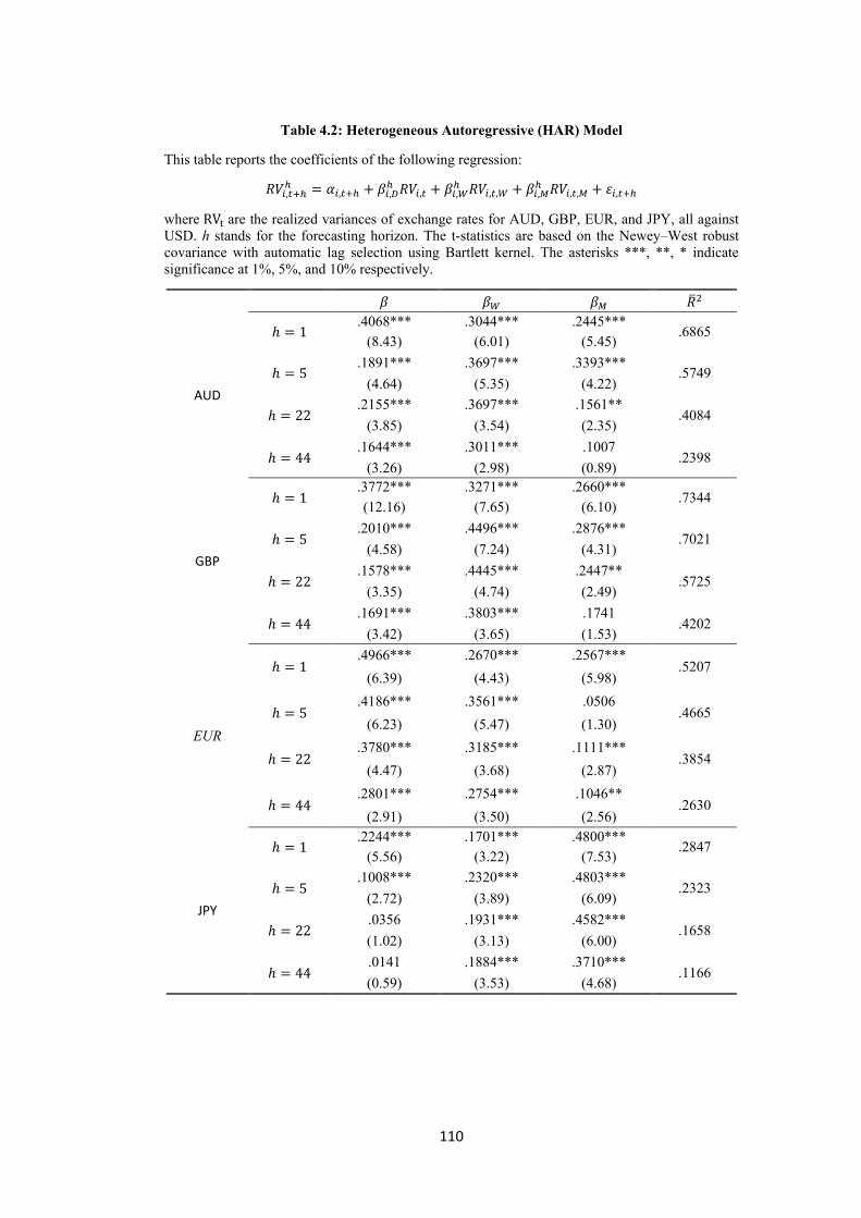
110

Table 4.2: Heterogeneous Autoregressive (HAR) Model

This table reports the coefficients of the following regression:

𝑅𝑉𝑖,𝑡+ℎℎ = 𝛼𝑖,𝑡+ℎ + 𝛽𝑖,𝐷

ℎ 𝑅𝑉𝑖,𝑡 + 𝛽𝑖,𝑊ℎ 𝑅𝑉𝑖,𝑡,𝑊 + 𝛽𝑖,𝑀

ℎ 𝑅𝑉𝑖,𝑡,𝑀 + 𝜀𝑖,𝑡+ℎ

where RVt are the realized variances of exchange rates for AUD, GBP, EUR, and JPY, all against

USD. h stands for the forecasting horizon. The t-statistics are based on the Newey–West robust

covariance with automatic lag selection using Bartlett kernel. The asterisks ***, **, * indicate

significance at 1%, 5%, and 10% respectively.

𝛽 𝛽𝑊 𝛽𝑀 �̅�2

AUD

ℎ = 1 .4068*** .3044*** .2445***

.6865 (8.43) (6.01) (5.45)

ℎ = 5 .1891*** .3697*** .3393***

.5749 (4.64) (5.35) (4.22)

ℎ = 22 .2155*** .3697*** .1561**

.4084 (3.85) (3.54) (2.35)

ℎ = 44 .1644*** .3011*** .1007

.2398 (3.26) (2.98) (0.89)

GBP

ℎ = 1 .3772*** .3271*** .2660***

.7344 (12.16) (7.65) (6.10)

ℎ = 5 .2010*** .4496*** .2876***

.7021 (4.58) (7.24) (4.31)

ℎ = 22 .1578*** .4445*** .2447**

.5725 (3.35) (4.74) (2.49)

ℎ = 44 .1691*** .3803*** .1741

.4202 (3.42) (3.65) (1.53)

EUR

ℎ = 1 .4966*** .2670*** .2567***

.5207 (6.39) (4.43) (5.98)

ℎ = 5 .4186*** .3561*** .0506

.4665 (6.23) (5.47) (1.30)

ℎ = 22 .3780*** .3185*** .1111***

.3854 (4.47) (3.68) (2.87)

ℎ = 44 .2801*** .2754*** .1046**

.2630 (2.91) (3.50) (2.56)

JPY

ℎ = 1 .2244*** .1701*** .4800***

.2847 (5.56) (3.22) (7.53)

ℎ = 5 .1008*** .2320*** .4803***

.2323 (2.72) (3.89) (6.09)

ℎ = 22 .0356 .1931*** .4582***

.1658 (1.02) (3.13) (6.00)

ℎ = 44 .0141 .1884*** .3710***

.1166 (0.59) (3.53) (4.68)

111

4.3.2. Semi-variance HAR

It is a well-established empirical regularity in the finance literature that negative

returns generally lead to higher future volatility than positive returns. While the

facts on the asymmetric effects are well-known in the equity markets (see, for

example, Andersen et al., 2007; Patton and Sheppard, 2015; Lahaye and Neely,

2016; Wang and Yang, 2017), the relevant studies present mixed results in the

foreign exchange market. For example, in contrast to equity markets, foreign

exchange market usually exhibits symmetric volatility, that is, the volatility impacts

of past positive and negative shocks are of similar magnitudes (Diebold and

Nerlove, 1989; Andersen et al., 2001; Hansen and Lunde, 2005; and Laurent et al.,

2011). However, in Wang and Yang (2009), the authors confirm the presence of

asymmetric volatility in the exchange rates, while the realized volatility of EUR

appears to be symmetric.

A key contribution of the recent econometric advances in modelling RV dynamics

is the improved volatility forecast performance. Corsi (2009) shows that the HAR

model generates more accurate forecasts than a true long-memory model with

fractional cointegration, while Patton and Sheppard (2015) show that the semi-

variance HAR model has better RV forecasts than the standard HAR and a RV-

based GJR-GARCH model. 36 Therefore, I utilize the same concepts of “good

volatility” and “bad volatility” as in Patton and Sheppard (2015), to explicitly test

for the presence of asymmetric effects in the FX market. Specifically, Barndorff-

Nielsen, Kinnebrock and Shephard (2010) introduce estimators that can capture

the variations only due to negative or positive returns using the realized semi-

variance (RS) estimator, which is defined as 𝑅𝑆𝑡+ = ∑ 𝑟𝑠,𝑡

2 𝐼{𝑟𝑠,𝑡 > 0}𝑚𝑠=1 and 𝑅𝑆𝑡

− =

∑ 𝑟𝑠,𝑡2 𝐼{𝑟𝑠,𝑡 < 0}𝑚

𝑠=1 and 𝐼 is the indicator function. These estimators provide a

complete decomposition of RV𝑡, in that RV𝑡 = 𝑅𝑆𝑡+ + 𝑅𝑆𝑡

−, which holds exactly for

any sampling interval m, as well as in the limit (Patton and Sheppard, 2015). I adopt

this technique of volatility decomposition for the following empirical analysis and

36 However, Bollerslev, Patton, and Quaedvlieg (2016) show that the HAR model with realized quarticity outperforms a range of models including the semi-variance HAR.

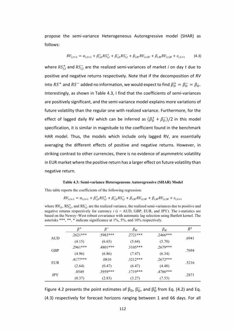
112

propose the semi-variance Heterogeneous Autoregressive model (SHAR) as

follows:

𝑅𝑉𝑖,𝑡+1 = 𝛼𝑖,𝑡+1 + 𝛽𝑖,𝐷+ 𝑅𝑆𝑖,𝑡

+ + 𝛽𝑖,𝐷− 𝑅𝑆𝑖,𝑡

− + 𝛽𝑖,𝑊𝑅𝑉𝑖,𝑡,𝑊 + 𝛽𝑖,𝑀𝑅𝑉𝑖,𝑡,𝑀 + 𝜀𝑖,𝑡+1 (4.3)

where 𝑅𝑆𝑖,𝑡+ and 𝑅𝑆𝑖,𝑡

− are the realized semi-variances of market i on day t due to

positive and negative returns respectively. Note that if the decomposition of RV

into 𝑅𝑆+ and 𝑅𝑆− added no information, we would expect to find 𝛽𝐷+ = 𝛽𝐷

− = 𝛽𝐷.

Interestingly, as shown in Table 4.3, I find that the coefficients of semi-variances

are positively significant, and the semi-variance model explains more variations of

future volatility than the regular one with realized variance. Furthermore, for the

effect of lagged daily RV which can be inferred as (𝛽𝐷+ + 𝛽𝐷

−)/2 in this model

specification, it is similar in magnitude to the coefficient found in the benchmark

HAR model. Thus, the models which include only lagged RV, are essentially

averaging the different effects of positive and negative returns. However, in

striking contrast to other currencies, there is no evidence of asymmetric volatility

in EUR market where the positive return has a larger effect on future volatility than

negative return.

Table 4.3: Semi-variance Heterogeneous Autoregressive (SHAR) Model

This table reports the coefficients of the following regression:

𝑅𝑉𝑖,𝑡+1 = 𝛼𝑖,𝑡+1 + 𝛽𝑖,𝐷+ 𝑅𝑆𝑖,𝑡

+ + 𝛽𝑖,𝐷− 𝑅𝑆𝑖,𝑡

− + 𝛽𝑖,𝑊𝑅𝑉𝑖,𝑡,𝑊 + 𝛽𝑖,𝑀𝑅𝑉𝑖,𝑡,𝑀 + 𝜀𝑖,𝑡+1

where RVi,t, RS𝑖,𝑡+ , and RS𝑖,𝑡

− are the realized variance, the realized semi-variances due to positive and

negative returns respectively for currency i (i = AUD, GBP, EUR, and JPY). The t-statistics are

based on the Newey–West robust covariance with automatic lag selection using Bartlett kernel. The

asterisks ***, **, * indicate significance at 1%, 5%, and 10% respectively.

𝛽+ 𝛽− 𝛽𝑊 𝛽𝑀 �̅�2

AUD .2621*** .5983*** .2721*** .2466***

.6941 (4.15) (6.65) (5.64) (5.70)

GBP .2961*** .4801*** .3105*** .2679***

.7694 (4.96) (6.86) (7.47) (6.34)

EUR .4177*** .0810 .3212*** .2672***

.5216 (2.64) (0.47) (6.47) (4.48)

JPY .0549 .3959*** .1719*** .4786***

.2871 (0.37) (2.83) (3.27) (7.53)

Figure 4.2 presents the point estimates of βD, βD−, and βD

+ from Eq. (4.2) and Eq.

(4.3) respectively for forecast horizons ranging between 1 and 66 days. For all

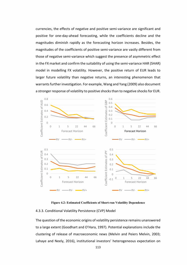
113

currencies, the effects of negative and positive semi-variance are significant and

positive for one-day-ahead forecasting, while the coefficients decline and the

magnitudes diminish rapidly as the forecasting horizon increases. Besides, the

magnitudes of the coefficients of positive semi-variance are vastly different from

those of negative semi-variance which suggest the presence of asymmetric effect

in the FX market and confirm the suitability of using the semi-variance HAR (SHAR)

model in modelling FX volatility. However, the positive return of EUR leads to

larger future volatility than negative returns, an interesting phenomenon that

warrants further investigation. For example, Wang and Yang (2009) also document

a stronger response of volatility to positive shocks than to negative shocks for EUR.

Figure 4.2: Estimated Coefficients of Short-run Volatility Dependence

4.3.3. Conditional Volatility Persistence (CVP) Model

The question of the economic origins of volatility persistence remains unanswered

to a large extent (Goodhart and O’Hara, 1997). Potential explanations include the

clustering of release of macroeconomic news (Melvin and Peiers Melvin, 2003;

Lahaye and Neely, 2016), institutional investors’ heterogeneous expectation on

0

0.2

0.4

0.6

0.8

0 1 5 22 44 66

Co

effi

cien

t Es

tim

ates

of

AU

D

Forecast Horizon

RV RV- RV+

0

0.1

0.2

0.3

0.4

0.5

0.6

0 1 5 22 44 66

Co

effi

cien

t Es

tim

ates

of

GB

P

Forecast Horizon

RV RV- RV+

0

0.1

0.2

0.3

0.4

0.5

0 1 5 22 44 66

Co

effi

cien

t Es

tim

ates

of

EUR

Forecast Horizon

RV RV- RV+

-0.1

0

0.1

0.2

0.3

0.4

0.5

0 1 5 22 44 66

Co

effi

cien

t Es

tim

ates

of

JPY

Forecast Horizon

RV RV- RV+

114

macroeconomic indicators (Hogan and Melvin, 1994) and heterogeneous trading

horizons (Müller et al., 1997), the incorporation of private information via trading

(Kyle, 1985; Admati and Pfleiderer, 1988; Ito et al., 1998), information flow and

market’s sensitivity to that information (Berger et al., 2009), the theory of Mixture

of Distribution Hypothesis (MDH) (Clark, 1973; Tauchen and Pitts, 1983; Andersen,

1996), and the conditional volatility persistence model which attributes the time-

varying volatility persistence into the changing market conditions, as captured by

daily return and volatility (Wang and Yang, 2017).37

In this section, I introduce the Conditional Volatility Persistence (CVP) model as

proposed in Wang and Yang (2017), which captures the long memory in volatility

while controlling for conditional variables. Specifically, I estimate a new empirical

model of the expected volatility persistence conditional on a set of observed

variables (i.e., return, volatility, and other proxy measures of trading activity), then

I calibrate and examine the volatility forecasting performance based on

conditional volatility persistence.

Namely, following Wang and Yang (2017) who attribute the time-varying volatility

persistence to the changing states of the market as captured by daily return and

volatility, I incorporate conditional volatility persistence into the HAR model

similarly. Here, considering that the negative returns are generally associated with

greater volatility than positive returns within a wide range of finance markets

(Patton and Sheppard, 2015; Wang and Yang, 2017), I decompose the exchange

rate returns into positive and negative returns, and examine their volatility

impacts separately. Then the modified HAR model which incorporates the

conditional volatility persistence can be written as follows:

37 Wang and Yang (2017) propose several dynamical mechanisms of volatility persistence, such as exogenous and endogenous information arrivals, the persistence of characteristics of price discovery, and uninformed trading, such as portfolio adjustments to lagged information shocks.

115

𝑅𝑉𝑖,𝑡+1 = 𝛼𝑖,𝑡+1 + 𝛽𝑖,𝑡𝑒 𝑅𝑉𝑖,𝑡 + 𝛽𝑖,W𝑅𝑉𝑖,𝑡,𝑊 + 𝛽𝑖,𝑀𝑅𝑉𝑖,𝑡,𝑀

+𝜃𝑖,𝑡𝑟𝑖,𝑡 + 𝜃𝑖,𝑊𝑟𝑖,𝑡,𝑊 + 𝜃𝑖,𝑀𝑟𝑖,𝑡,𝑀 + 𝜀𝑖,𝑡+1 (4.4)

where 𝛽𝑖,𝑡𝑒 = 𝛽𝑖

0 + 𝛽𝑖−𝑟𝑖,𝑡

− + 𝛽𝑖+𝑟𝑖,𝑡

+ + 𝛽𝑖𝑅𝑉𝑅𝑉𝑖,𝑡 is called the conditional volatility

persistence (CVP) as defined earlier. The weekly and monthly realized variance are

calculated as RVi,t,W =1

4∑ RVi,t−k

5k=2 and RVi,t,M =

1

17∑ RVi,t−k

22k=6 respectively.

ri,t,W and ri,t,M are weekly and monthly return, which are defined similarly and

utilized to capture the heterogeneous return impacts.

By incorporating time-varying conditional volatility persistence into the HAR

model, I can examine the dynamic “leverage effect” while capturing long memory

in volatility (Wang and Yang, 2017). In Table 4.4, I find that the proposed CVP

model reduces the sizes of all coefficients in HAR model, therefore, reducing the

estimated long-run dependence of volatility as documented earlier. While not

reported here, the Wald-statistics resoundingly reject the null hypothesis of 𝛽− =

𝛽+ = 𝛽𝑅𝑉 = 0; both the adjusted R-squared and information criteria (i.e., AIC and

BIC) are in favour of the conditional HAR model, namely, the CVP model, over the

regular one. While the stylized facts on the asymmetric effects are well-

documented in the equity market, the relevant studies present mixed results in

the foreign exchange market. The results presented in Table 4.4 suggest that there

is mixed evidence on asymmetric effects in the FX market, i.e. the volatility impact

of negative return is stronger than that of positive return for AUD, GBP, and JPY,

while for EUR, it responds more strongly to past positive shocks.38

38 As stated earlier in Section 4.3.2, similar results have been documented in Wang and Yang (2009).

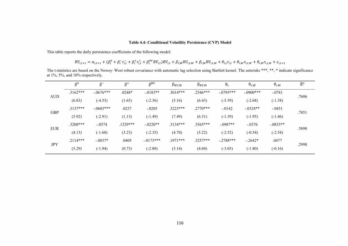
116

Table 4.4: Conditional Volatility Persistence (CVP) Model


𝑅𝑉𝑖,𝑡+1 = 𝛼𝑖,𝑡+1 + (𝛽𝑖0 + 𝛽𝑖

−𝑟𝑖,𝑡− + 𝛽𝑖

+𝑟𝑖,𝑡+ + 𝛽𝑖

𝑅𝑉𝑅𝑉𝑖,𝑡)𝑅𝑉𝑖,𝑡 + 𝛽𝑖,W𝑅𝑉𝑖,𝑡,𝑊 + 𝛽𝑖,𝑀𝑅𝑉𝑖,𝑡,𝑀 + 𝜃𝑖,𝑡𝑟𝑖,𝑡 + 𝜃𝑖,𝑊𝑟𝑖,𝑡,𝑊 + 𝜃𝑖,𝑀𝑟𝑖,𝑡,𝑀 + 𝜀𝑖,𝑡+1

The t-statistics are based on the Newey–West robust covariance with automatic lag selection using Bartlett kernel. The asterisks ***, **, * indicate significance

at 1%, 5%, and 10% respectively.

β0 β− β+ βRV βRV,W βRV,M θr θr,W θr,M R̅2

AUD .3162*** -.0676*** .0248* -.0183** .3014*** .2546*** -.0795*** -.0900*** -.0781

.7606 (6.83) (-4.53) (1.65) (-2.36) (5.16) (6.43) (-5.59) (-2.68) (-1.38)

GBP .3137*** -.0603*** .0237 -.0205 .3223*** .2770*** -.0142 -.0324** -.0451

.7851 (5.92) (-2.91) (1.13) (-1.49) (7.49) (6.31) (-1.39) (-1.95) (-1.46)

EUR .3208*** -.0574 .1329*** -.0220** .3134*** .3565*** -.0987** -.0376 -.0833**

.5890 (4.13) (-1.60) (3.23) (-2.35) (4.70) (5.22) (-2.52) (-0.54) (-2.54)

JPY .2114*** -.0837* .0405 -.0173*** .1971*** .3257*** -.2788*** -.2642* .0477

.2998 (5.29) (-1.94) (0.73) (-2.80) (3.14) (4.60) (-3.05) (-1.80) (-0.16)

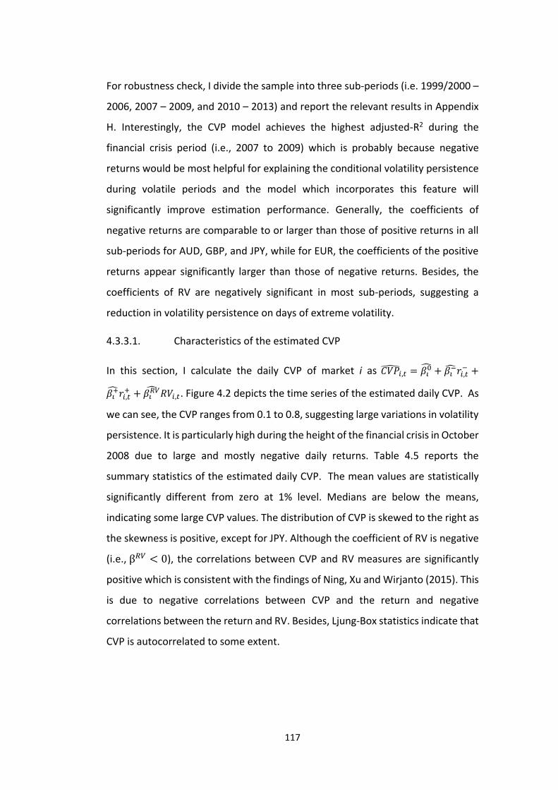
117

For robustness check, I divide the sample into three sub-periods (i.e. 1999/2000 –

2006, 2007 – 2009, and 2010 – 2013) and report the relevant results in Appendix

H. Interestingly, the CVP model achieves the highest adjusted-R2 during the

financial crisis period (i.e., 2007 to 2009) which is probably because negative

returns would be most helpful for explaining the conditional volatility persistence

during volatile periods and the model which incorporates this feature will

significantly improve estimation performance. Generally, the coefficients of

negative returns are comparable to or larger than those of positive returns in all

sub-periods for AUD, GBP, and JPY, while for EUR, the coefficients of the positive

returns appear significantly larger than those of negative returns. Besides, the

coefficients of RV are negatively significant in most sub-periods, suggesting a

reduction in volatility persistence on days of extreme volatility.

4.3.3.1. Characteristics of the estimated CVP

In this section, I calculate the daily CVP of market i as 𝐶𝑉�̂�𝑖,𝑡 = 𝛽𝑖0̂ + 𝛽𝑖

−̂𝑟𝑖,𝑡− +

𝛽𝑖+̂𝑟𝑖,𝑡

+ + 𝛽𝑖𝑅�̂�𝑅𝑉𝑖,𝑡. Figure 4.2 depicts the time series of the estimated daily CVP. As

we can see, the CVP ranges from 0.1 to 0.8, suggesting large variations in volatility

persistence. It is particularly high during the height of the financial crisis in October

2008 due to large and mostly negative daily returns. Table 4.5 reports the

summary statistics of the estimated daily CVP. The mean values are statistically

significantly different from zero at 1% level. Medians are below the means,

indicating some large CVP values. The distribution of CVP is skewed to the right as

the skewness is positive, except for JPY. Although the coefficient of RV is negative

(i.e., β𝑅𝑉 < 0), the correlations between CVP and RV measures are significantly

positive which is consistent with the findings of Ning, Xu and Wirjanto (2015). This

is due to negative correlations between CVP and the return and negative

correlations between the return and RV. Besides, Ljung-Box statistics indicate that

CVP is autocorrelated to some extent.

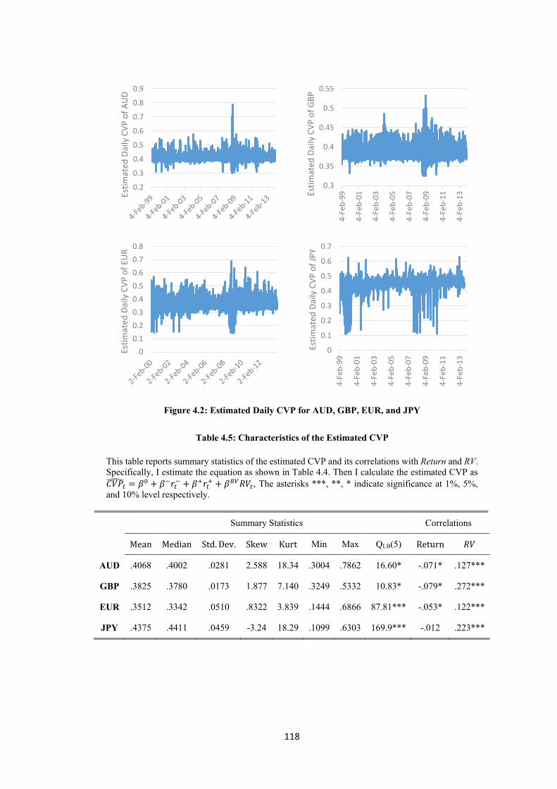
118

Figure 4.2: Estimated Daily CVP for AUD, GBP, EUR, and JPY

Table 4.5: Characteristics of the Estimated CVP

This table reports summary statistics of the estimated CVP and its correlations with Return and RV.

Specifically, I estimate the equation as shown in Table 4.4. Then I calculate the estimated CVP as

𝐶𝑉�̂�𝑡 = 𝛽0 + 𝛽−𝑟𝑡− + 𝛽+𝑟𝑡

+ + 𝛽𝑅𝑉𝑅𝑉𝑡, The asterisks ***, **, * indicate significance at 1%, 5%,

and 10% level respectively.

Summary Statistics Correlations

Mean Median Std. Dev. Skew Kurt Min Max QLB(5) Return 𝑅𝑉

AUD .4068 .4002 .0281 2.588 18.34 .3004 .7862 16.60* -.071* .127***

GBP .3825 .3780 .0173 1.877 7.140 .3249 .5332 10.83* -.079* .272***

EUR .3512 .3342 .0510 .8322 3.839 .1444 .6866 87.81*** -.053* .122***

JPY .4375 .4411 .0459 -3.24 18.29 .1099 .6303 169.9*** -.012 .223***

0.2

0.3

0.4

0.5

0.6

0.7

0.8

0.9

Esti

mat

ed D

aily

CV

P o

f A

UD

0.3

0.35

0.4

0.45

0.5

0.55

4-F

eb-9

9

4-F

eb-0

1

4-F

eb-0

3

4-F

eb-0

5

4-F

eb-0

7

4-F

eb-0

9

4-F

eb-1

1

4-F

eb-1

3Esti

mat

ed D

aily

CV

P o

f G

BP

0

0.1

0.2

0.3

0.4

0.5

0.6

0.7

0.8

Esti

mat

ed D

aily

CV

P o

f EU

R

0

0.1

0.2

0.3

0.4

0.5

0.6

0.7

4-F

eb-9

9

4-F

eb-0

1

4-F

eb-0

3

4-F

eb-0

5

4-F

eb-0

7

4-F

eb-0

9

4-F

eb-1

1

4-F

eb-1

3

Esti

mat

ed D

aily

CV

P o

f JP

Y

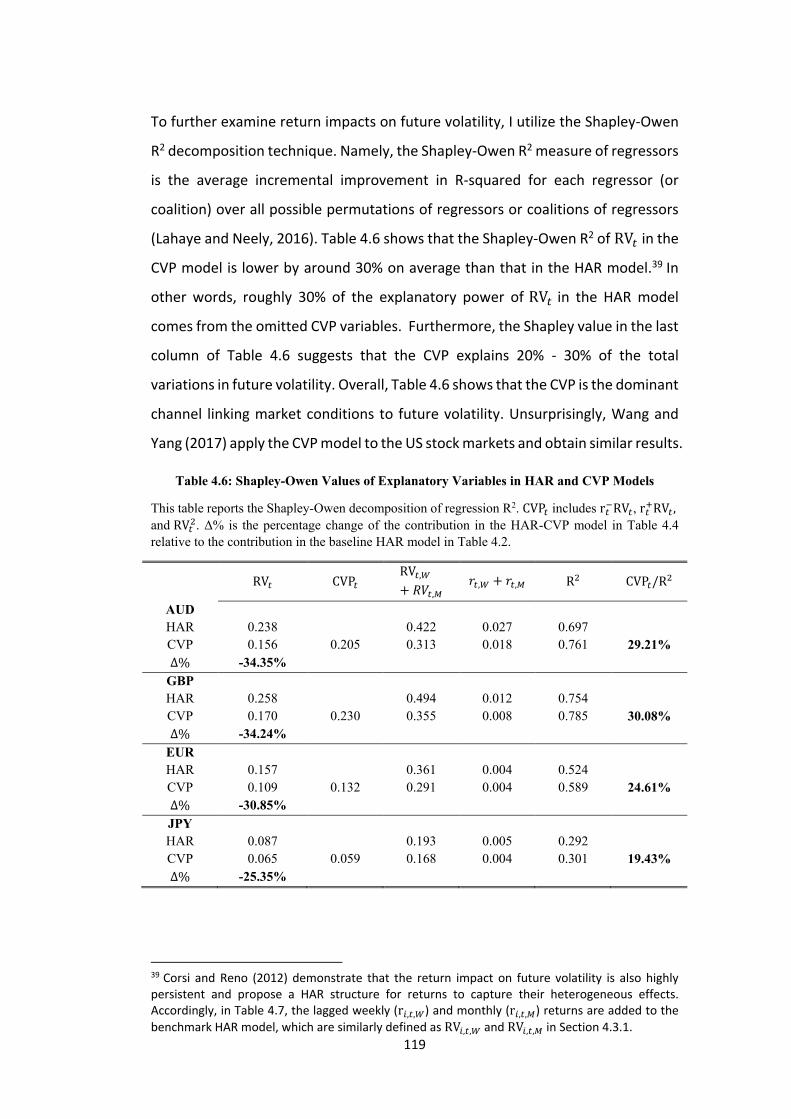
119

To further examine return impacts on future volatility, I utilize the Shapley-Owen

R2 decomposition technique. Namely, the Shapley-Owen R2 measure of regressors

is the average incremental improvement in R-squared for each regressor (or

coalition) over all possible permutations of regressors or coalitions of regressors

(Lahaye and Neely, 2016). Table 4.6 shows that the Shapley-Owen R2 of RV𝑡 in the

CVP model is lower by around 30% on average than that in the HAR model.39 In

other words, roughly 30% of the explanatory power of RV𝑡 in the HAR model

comes from the omitted CVP variables. Furthermore, the Shapley value in the last

column of Table 4.6 suggests that the CVP explains 20% - 30% of the total

variations in future volatility. Overall, Table 4.6 shows that the CVP is the dominant

channel linking market conditions to future volatility. Unsurprisingly, Wang and

Yang (2017) apply the CVP model to the US stock markets and obtain similar results.

Table 4.6: Shapley-Owen Values of Explanatory Variables in HAR and CVP Models

This table reports the Shapley-Owen decomposition of regression R2. CVP𝑡 includes r𝑡−RV𝑡, r𝑡

+RV𝑡 ,

and RV𝑡2. Δ% is the percentage change of the contribution in the HAR-CVP model in Table 4.4

relative to the contribution in the baseline HAR model in Table 4.2.

RV𝑡 CVP𝑡 RV𝑡,𝑊

+ 𝑅𝑉𝑡,𝑀 𝑟𝑡,𝑊 + 𝑟𝑡,𝑀 R2 CVP𝑡/R2

AUD

HAR 0.238 0.422 0.027 0.697

CVP 0.156 0.205 0.313 0.018 0.761 29.21%

∆% -34.35%

GBP

HAR 0.258 0.494 0.012 0.754

CVP 0.170 0.230 0.355 0.008 0.785 30.08%

∆% -34.24%

EUR

HAR 0.157 0.361 0.004 0.524

CVP 0.109 0.132 0.291 0.004 0.589 24.61%

∆% -30.85%

JPY

HAR 0.087 0.193 0.005 0.292

CVP 0.065 0.059 0.168 0.004 0.301 19.43%

∆% -25.35%

39 Corsi and Reno (2012) demonstrate that the return impact on future volatility is also highly persistent and propose a HAR structure for returns to capture their heterogeneous effects. Accordingly, in Table 4.7, the lagged weekly (r𝑖,𝑡,𝑊) and monthly (r𝑖,𝑡,𝑀) returns are added to the

benchmark HAR model, which are similarly defined as RV𝑖,𝑡,𝑊 and RV𝑖,𝑡,𝑀 in Section 4.3.1.

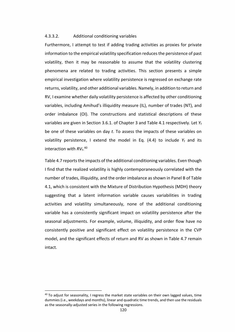
120

4.3.3.2. Additional conditioning variables

Furthermore, I attempt to test if adding trading activities as proxies for private

information to the empirical volatility specification reduces the persistence of past

volatility, then it may be reasonable to assume that the volatility clustering

phenomena are related to trading activities. This section presents a simple

empirical investigation where volatility persistence is regressed on exchange rate

returns, volatility, and other additional variables. Namely, in addition to return and

RV, I examine whether daily volatility persistence is affected by other conditioning

variables, including Amihud’s illiquidity measure (IL), number of trades (NT), and

order imbalance (OI). The constructions and statistical descriptions of these

variables are given in Section 3.6.1. of Chapter 3 and Table 4.1 respectively. Let Yt

be one of these variables on day t. To assess the impacts of these variables on

volatility persistence, I extend the model in Eq. (4.4) to include Yt and its

interaction with RVt.40

Table 4.7 reports the impacts of the additional conditioning variables. Even though

I find that the realized volatility is highly contemporaneously correlated with the

number of trades, illiquidity, and the order imbalance as shown in Panel B of Table

4.1, which is consistent with the Mixture of Distribution Hypothesis (MDH) theory

suggesting that a latent information variable causes variabilities in trading

activities and volatility simultaneously, none of the additional conditioning

variable has a consistently significant impact on volatility persistence after the

seasonal adjustments. For example, volume, illiquidity, and order flow have no

consistently positive and significant effect on volatility persistence in the CVP

model, and the significant effects of return and RV as shown in Table 4.7 remain

intact.

40 To adjust for seasonality, I regress the market state variables on their own lagged values, time dummies (i.e., weekdays and months), linear and quadratic time trends, and then use the residuals as the seasonally-adjusted series in the following regressions.

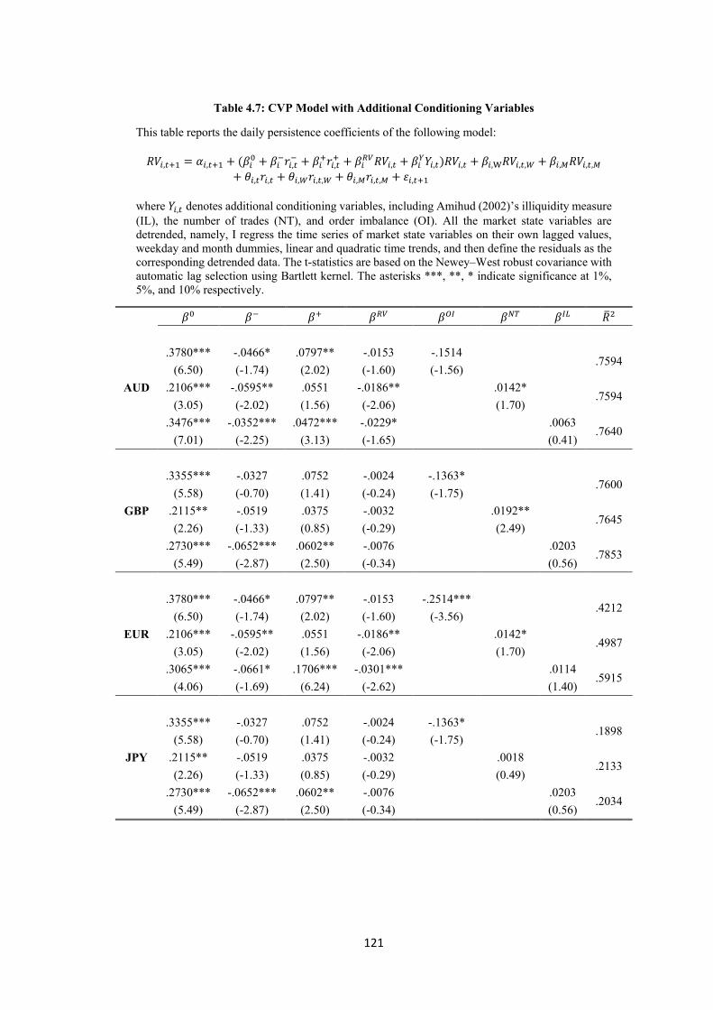
121

Table 4.7: CVP Model with Additional Conditioning Variables


𝑅𝑉𝑖,𝑡+1 = 𝛼𝑖,𝑡+1 + (𝛽𝑖0 + 𝛽𝑖



𝑅𝑉𝑅𝑉𝑖,𝑡 + 𝛽𝑖𝑌𝑌𝑖,𝑡)𝑅𝑉𝑖,𝑡 + 𝛽𝑖,W𝑅𝑉𝑖,𝑡,𝑊 + 𝛽𝑖,𝑀𝑅𝑉𝑖,𝑡,𝑀

+ 𝜃𝑖,𝑡𝑟𝑖,𝑡 + 𝜃𝑖,𝑊𝑟𝑖,𝑡,𝑊 + 𝜃𝑖,𝑀𝑟𝑖,𝑡,𝑀 + 𝜀𝑖,𝑡+1

where 𝑌𝑖,𝑡 denotes additional conditioning variables, including Amihud (2002)’s illiquidity measure

(IL), the number of trades (NT), and order imbalance (OI). All the market state variables are

detrended, namely, I regress the time series of market state variables on their own lagged values,

weekday and month dummies, linear and quadratic time trends, and then define the residuals as the

corresponding detrended data. The t-statistics are based on the Newey–West robust covariance with

automatic lag selection using Bartlett kernel. The asterisks ***, **, * indicate significance at 1%,

5%, and 10% respectively.

𝛽0 𝛽− 𝛽+ 𝛽𝑅𝑉 𝛽𝑂𝐼 𝛽𝑁𝑇 𝛽𝐼𝐿 �̅�2

AUD

.3780*** -.0466* .0797** -.0153 -.1514 .7594

(6.50) (-1.74) (2.02) (-1.60) (-1.56)

.2106*** -.0595** .0551 -.0186** .0142* .7594

(3.05) (-2.02) (1.56) (-2.06) (1.70)

.3476*** -.0352*** .0472*** -.0229* .0063 .7640

(7.01) (-2.25) (3.13) (-1.65) (0.41)

GBP

.3355*** -.0327 .0752 -.0024 -.1363* .7600

(5.58) (-0.70) (1.41) (-0.24) (-1.75)

.2115** -.0519 .0375 -.0032 .0192** .7645

(2.26) (-1.33) (0.85) (-0.29) (2.49)

.2730*** -.0652*** .0602** -.0076 .0203 .7853

(5.49) (-2.87) (2.50) (-0.34) (0.56)

EUR

.3780*** -.0466* .0797** -.0153 -.2514*** .4212

(6.50) (-1.74) (2.02) (-1.60) (-3.56)

.2106*** -.0595** .0551 -.0186** .0142* .4987

(3.05) (-2.02) (1.56) (-2.06) (1.70)

.3065*** -.0661* .1706*** -.0301*** .0114 .5915

(4.06) (-1.69) (6.24) (-2.62) (1.40)

JPY

.3355*** -.0327 .0752 -.0024 -.1363* .1898

(5.58) (-0.70) (1.41) (-0.24) (-1.75)

.2115** -.0519 .0375 -.0032 .0018 .2133

(2.26) (-1.33) (0.85) (-0.29) (0.49)

.2730*** -.0652*** .0602** -.0076 .0203 .2034

(5.49) (-2.87) (2.50) (-0.34) (0.56)

122

4.3.4. Economic Value of Volatility Timing

In this section, I estimate the economic benefits of volatility forecasting models

using a number of evaluation metrics. First, in terms of economic gains, I compute

the realized utility that a given volatility model generates over that from the static

one. Namely, the main purpose is to estimate the fee that an investor would be

willing to pay for switching from a static risk model. Second, I examine the ex-post

performance of optimal portfolio with predictive volatility (i.e. average portfolio

returns, volatility, and the Sharpe ratio). If the dynamic volatility models generate

more accurate volatility forecasts, then the investor would gain from dynamically

rebalancing the optimal portfolio based on the signal of the predicted volatility.

To compare the realized utility across risk models, I consider the simplest possible

utility-based framework, namely, an investor with mean-variance preferences

investing in an asset with time-varying volatility and a constant Sharpe ratio.41

The major advantages of this “realized utility” approach lie in the fact that by

assuming a constant Sharpe ratio, I don’t have to predict future exchange rate

movements, which is difficult if possible at all, given the fact that exchange rates

generally follow a random walk process (Meese and Rogoff, 1983). Furthermore,

the “realized utility” approach is based on the daily estimates of volatility and is

very easy to implement. Last but not least, this non-parametric approach also

mitigates the impact of estimation risk or parameter learning which would

probably lead to misleading allocations.

To empirically conduct the economic evaluations of volatility forecasting models,

I consider a risk-averse investor with mean-variance preferences, who allocates

her wealth into one risky asset (i.e., a single currency pair) and one risk-free asset

(i.e. the US treasury bond). The specification of one risk asset in the portfolio is

similar to Nolte and Xu (2005) and Bollerslev et al. (2017), which avoids covariance

forecasting in multivariate settings and controls for information spillovers across

41 However, as explained in Bollerslev et al. (2017), the same setup readily extends to allow for time-varying Sharpe ratios as long as the temporal variation of Sharpe ratio is independent of the conditional risk.

123

different assets. The economic explanation behind this strategy is intuitive: given

the expected return, when the volatility level is high (low), the investor allocates

less (more) wealth into the risky asset and yields higher risk-adjusted return. If

taking account of the conditional volatility persistence leads to more accurate

volatility forecasting, then the investor would improve her portfolio performance

by dynamically rebalancing the portfolio based on the signal of the predicted

volatility. Different from existing studies which compare dynamic and static

strategies (Fleming et al., 2001), dynamic strategies based on returns sampled at

high frequency and daily frequency (Fleming et al., 2003), dynamic strategies

utilizing the conventional realized variance and jump-robust realized variance

measures (Nolte and Xu, 2015), the analysis in this chapter compares the

performances of variants of HAR models all of which use high frequency

information and build upon dynamic structure. Generally, this study is closely

related to Bollerslev et al. (2017) which compares multiple RV-based HAR models.

However, I confirm that the CVP model, which explicitly links market conditions to

future volatility persistence, beats other RV-based HAR models in terms of

statistical significance and economic value.

Namely, I consider an investor with mean-variance preferences that trades a risky

asset with a constant Sharpe ratio, so the investor’s optimal portfolio naturally

adjusts the position size to keep a constant volatility (which will also depend on

the investor’s risk aversion). For concreteness and simplicity, I take the Sharpe

ratio to be SR = 0.3 and the risk aversion to be γ = 3, which results in a specified

target volatility of 0.1 or 10%.42 Hence, risk models that help the investor achieve

more accurate forecasts of future volatilities are associated with higher levels of

utility. Here, I empirically evaluate the average realized utility per unit of wealth

(UoW) for each risk model by summing the corresponding realized expressions

42 In fact, the number of 10% volatility level is in the right ballpark for many target volatility funds, according to Bollerslev et al. (2017).

124

over the same rolling out-of-sample forecasts (For short, we can simply call this

the “realized utility” as in Bollerslev et al. (2017).): 43

𝑈𝑜𝑊𝜃 =1

𝑇∑ (3%

√𝑅𝑉𝑡+1

√𝐸𝑡𝜃(𝑅𝑉𝑡+1)

− 1.5%𝑅𝑉𝑡+1

𝐸𝑡𝜃(𝑅𝑉𝑡+1)

)𝑇𝑡=1 (4.5)

where 𝑅𝑉𝑡+1 and 𝐸𝑡(𝑅𝑉𝑡+1) are the observed and predicted realized variance on

day t+1 respectively. Mathematically, a perfect risk prediction model would lead

to 1.50% utility according to Eq. (4.5). The realized utility obviously depends on

the specific risk model 𝜃, since each risk model gives rise to different predictions

𝐸𝑡𝜃(𝑅𝑉𝑡+1), therefore leading to different position sizes. Since the expected return

has been substituted, this measure of realized utility only depends on each risk

model’s ability to correctly target volatility. Importantly, this approach eliminates

the noise from random return realizations, allowing us to meaningfully compare

different risk models based only on the actual realized volatilities for different

assets (Bollerslev et al., 2017).

4.4. Empirical Results

4.4.1. Out-of-sample Forecasting Performance

I firstly estimate the model parameters using the first 5 years of observations as

the in-sample period, and then use the rest of the sample as the out-of-sample

period. All of the forecasts are generated using rolling WLS regressions and

parameter estimates are updated daily. Namely, forecasts are based on 5-year

rolling windows, starting from January 1999 for AUD, GBP, and JPY, while from

January 2000 for EUR, resulting in more than 2,000 daily observations as the

forecasting subsample. No restrictions on the parameters are imposed and

therefore forecasts are occasionally negative. 44 Forecasting performance is

evaluated based on two loss functions: the quasi-likelihood function

QLIKE(RV𝑡 , RV̂𝑡) =RV𝑡

RV̂𝑡− ln (

RV𝑡

RV̂𝑡) − 1 and the logarithmic mean-squared errors

43 For a more detailed introduction to the derivation of the expression of average realized utility per unit of wealth (UoW), please refer to Section 6 of quantifying the utility benefit of risk models in Bollerslev et al. (2017). 44 Following Wang and Yang (2017), an “insanity filter” is used to replace a negative RV forecast with the lowest RV in the rolling window.

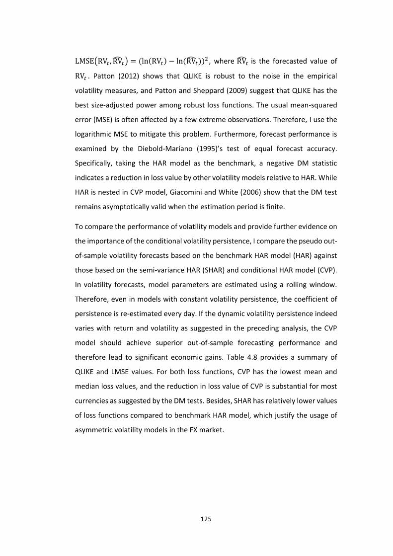
125

LMSE(RV𝑡 , RV̂𝑡) = (ln(RV𝑡) − ln (RV̂𝑡))2 , where RV̂𝑡 is the forecasted value of

RV𝑡 . Patton (2012) shows that QLIKE is robust to the noise in the empirical

volatility measures, and Patton and Sheppard (2009) suggest that QLIKE has the

best size-adjusted power among robust loss functions. The usual mean-squared

error (MSE) is often affected by a few extreme observations. Therefore, I use the

logarithmic MSE to mitigate this problem. Furthermore, forecast performance is

examined by the Diebold-Mariano (1995)’s test of equal forecast accuracy.

Specifically, taking the HAR model as the benchmark, a negative DM statistic

indicates a reduction in loss value by other volatility models relative to HAR. While

HAR is nested in CVP model, Giacomini and White (2006) show that the DM test

remains asymptotically valid when the estimation period is finite.

To compare the performance of volatility models and provide further evidence on

the importance of the conditional volatility persistence, I compare the pseudo out-

of-sample volatility forecasts based on the benchmark HAR model (HAR) against

those based on the semi-variance HAR (SHAR) and conditional HAR model (CVP).

In volatility forecasts, model parameters are estimated using a rolling window.

Therefore, even in models with constant volatility persistence, the coefficient of

persistence is re-estimated every day. If the dynamic volatility persistence indeed

varies with return and volatility as suggested in the preceding analysis, the CVP

model should achieve superior out-of-sample forecasting performance and

therefore lead to significant economic gains. Table 4.8 provides a summary of

QLIKE and LMSE values. For both loss functions, CVP has the lowest mean and

median loss values, and the reduction in loss value of CVP is substantial for most

currencies as suggested by the DM tests. Besides, SHAR has relatively lower values

of loss functions compared to benchmark HAR model, which justify the usage of

asymmetric volatility models in the FX market.

126

Table 4.8: Forecasting Performance Evaluation

This table reports the average, median, and standard deviation of the loss functions QLIKE and

LMSE for the HAR model, the semi-variance HAR model (SHAR), and the conditional HAR model

(CVP) using the exchange rates of AUD, GBP, EUR, and JPY, all against USD. DM stat is the

Diebold-Mariano (1995)’s test for the equality of forecast accuracy of two forecasts. Here, taking

the HAR model as the benchmark, a negative DM statistic indicates a reduction in loss value relative

to HAR.

HAR SHAR CVP

QLIKE LMSE QLIKE LMSE QLIKE LMSE

AUD

Average 0.2129 0.1243 0.2111 0.1234 0.2083 0.1222

Median 0.0779 0.0395 0.0768 0.0390 0.0752 0.0382

St Dev 0.4127 0.3302 0.4092 0.3256 0.4040 0.3188

DM Stat 0 0 -4.33*** -3.18*** -8.26*** -4.13***

GBP

Average 0.1478 0.0804 0.1458 0.0801 0.1429 0.0800

Median 0.0597 0.0159 0.0568 0.0147 0.0525 0.0128

St Dev 0.2147 0.2302 0.2104 0.2288 0.2040 0.2266

DM Stat 0 0 -1.77* -1.72* -1.82* -1.83*

EUR

Average 0.5392 0.3491 0.5206 0.3345 0.4920 0.3210

Median 0.2402 0.1415 0.2385 0.1265 0.2179 0.1140

St Dev 0.7997 0.7411 0.7937 0.7310 0.8088 0.7562

DM Stat 0 0 -1.78* -1.56 -2.78** -1.76*

JPY

Average 1.0115 0.8968 0.9633 0.8724 0.9922 0.8359

Median 0.4907 0.2671 0.4561 0.2582 0.4769 0.2449

St Dev 1.4504 2.2453 1.4449 2.2385 1.4482 2.2282

DM Stat 0 0 -1.62* -1.48 -1.54 -1.66*

127

4.4.2. Realized Utility of Volatility Timing

Firstly, I investigate the utility benefits of the different risk models in the absence

of transaction costs by calculating the realized utilities as given directly by Eq. (3.5).

I then incorporate reasonable transaction cost estimates into the analysis, along

with noise-robust realized variance measures in the robustness analysis section.

The results rely on the same rolling estimates for the different risk models

underlying the daily predictive out-of-sample forecasts. For comparison purposes,

I also include the results for additional simple benchmark models.

Specifically, the first column on the top of Table 4.9 (i.e., the full sample) reports

the realized utilities from using static risk models, namely, the in-sample mean of

volatility. Doing so achieves a realized utility of 0.75% on average across all

currencies, half the 1.50% maximum utility for the perfectly targeted daily

positions. Meanwhile, as the second column shows, even a simple dynamic risk

targeting strategy based on the 21-day rolling average of realized variance

generates quite substantial gains vis-à-vis the static position reported in the first

column. The third to fifth columns report the realized utilities obtained from using

the predicted realized variances based on classic HAR model, semi-variance HAR

(SHAR) model, and conditional HAR (CVP) model respectively. As previously noted,

perfectly targeting the daily volatility would result in a realized utility of 1.50%. By

comparison, a risk model that takes the conditional volatility persistence into

account would result in an average realized utility of 1.26%. This latter number, of

course, is quite close to the utilities obtained from each of the practically feasible

RV-based risk models.

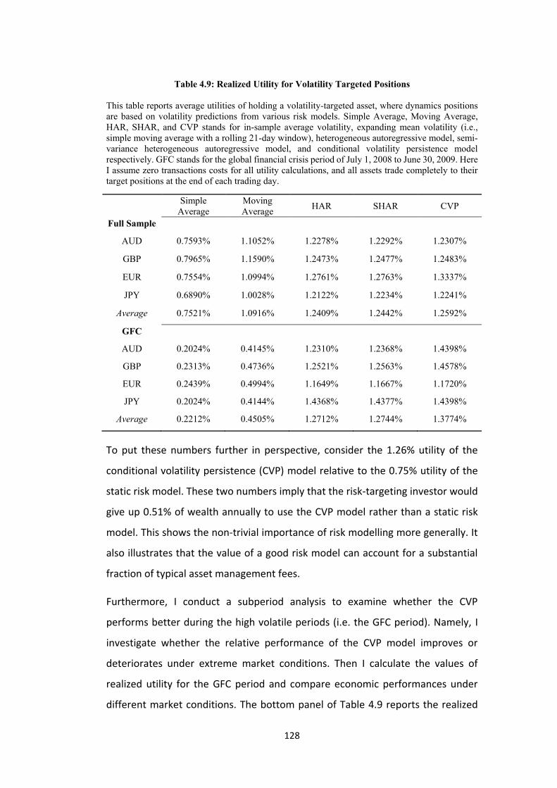
128

Table 4.9: Realized Utility for Volatility Targeted Positions

This table reports average utilities of holding a volatility-targeted asset, where dynamics positions

are based on volatility predictions from various risk models. Simple Average, Moving Average,

HAR, SHAR, and CVP stands for in-sample average volatility, expanding mean volatility (i.e.,

simple moving average with a rolling 21-day window), heterogeneous autoregressive model, semi-

variance heterogeneous autoregressive model, and conditional volatility persistence model

respectively. GFC stands for the global financial crisis period of July 1, 2008 to June 30, 2009. Here

I assume zero transactions costs for all utility calculations, and all assets trade completely to their

target positions at the end of each trading day.

Simple

Average

Moving

Average HAR SHAR CVP

Full Sample

AUD 0.7593% 1.1052% 1.2278% 1.2292% 1.2307%

GBP 0.7965% 1.1590% 1.2473% 1.2477% 1.2483%

EUR 0.7554% 1.0994% 1.2761% 1.2763% 1.3337%

JPY 0.6890% 1.0028% 1.2122% 1.2234% 1.2241%

Average 0.7521% 1.0916% 1.2409% 1.2442% 1.2592%

GFC

AUD 0.2024% 0.4145% 1.2310% 1.2368% 1.4398%

GBP 0.2313% 0.4736% 1.2521% 1.2563% 1.4578%

EUR 0.2439% 0.4994% 1.1649% 1.1667% 1.1720%

JPY 0.2024% 0.4144% 1.4368% 1.4377% 1.4398%

Average 0.2212% 0.4505% 1.2712% 1.2744% 1.3774%

To put these numbers further in perspective, consider the 1.26% utility of the

conditional volatility persistence (CVP) model relative to the 0.75% utility of the

static risk model. These two numbers imply that the risk-targeting investor would

give up 0.51% of wealth annually to use the CVP model rather than a static risk

model. This shows the non-trivial importance of risk modelling more generally. It

also illustrates that the value of a good risk model can account for a substantial

fraction of typical asset management fees.

Furthermore, I conduct a subperiod analysis to examine whether the CVP

performs better during the high volatile periods (i.e. the GFC period). Namely, I

investigate whether the relative performance of the CVP model improves or

deteriorates under extreme market conditions. Then I calculate the values of

realized utility for the GFC period and compare economic performances under

different market conditions. The bottom panel of Table 4.9 reports the realized

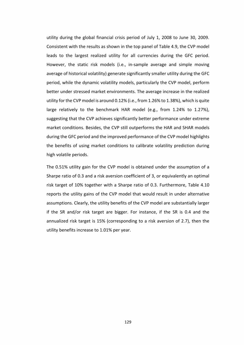
129

utility during the global financial crisis period of July 1, 2008 to June 30, 2009.

Consistent with the results as shown in the top panel of Table 4.9, the CVP model

leads to the largest realized utility for all currencies during the GFC period.

However, the static risk models (i.e., in-sample average and simple moving

average of historical volatility) generate significantly smaller utility during the GFC

period, while the dynamic volatility models, particularly the CVP model, perform

better under stressed market environments. The average increase in the realized

utility for the CVP model is around 0.12% (i.e., from 1.26% to 1.38%), which is quite

large relatively to the benchmark HAR model (e.g., from 1.24% to 1.27%),

suggesting that the CVP achieves significantly better performance under extreme

market conditions. Besides, the CVP still outperforms the HAR and SHAR models

during the GFC period and the improved performance of the CVP model highlights

the benefits of using market conditions to calibrate volatility prediction during

high volatile periods.

The 0.51% utility gain for the CVP model is obtained under the assumption of a

Sharpe ratio of 0.3 and a risk aversion coefficient of 3, or equivalently an optimal

risk target of 10% together with a Sharpe ratio of 0.3. Furthermore, Table 4.10

reports the utility gains of the CVP model that would result in under alternative

assumptions. Clearly, the utility benefits of the CVP model are substantially larger

if the SR and/or risk target are bigger. For instance, if the SR is 0.4 and the

annualized risk target is 15% (corresponding to a risk aversion of 2.7), then the

utility benefits increase to 1.01% per year.

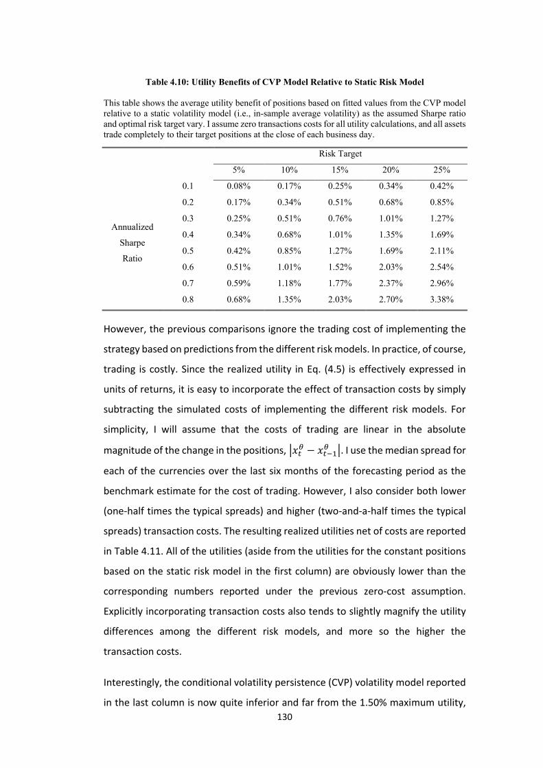
130

Table 4.10: Utility Benefits of CVP Model Relative to Static Risk Model

This table shows the average utility benefit of positions based on fitted values from the CVP model

relative to a static volatility model (i.e., in-sample average volatility) as the assumed Sharpe ratio

and optimal risk target vary. I assume zero transactions costs for all utility calculations, and all assets

trade completely to their target positions at the close of each business day.

Risk Target

5% 10% 15% 20% 25%

Annualized

Sharpe

Ratio

0.1 0.08% 0.17% 0.25% 0.34% 0.42%

0.2 0.17% 0.34% 0.51% 0.68% 0.85%

0.3 0.25% 0.51% 0.76% 1.01% 1.27%

0.4 0.34% 0.68% 1.01% 1.35% 1.69%

0.5 0.42% 0.85% 1.27% 1.69% 2.11%

0.6 0.51% 1.01% 1.52% 2.03% 2.54%

0.7 0.59% 1.18% 1.77% 2.37% 2.96%

0.8 0.68% 1.35% 2.03% 2.70% 3.38%

However, the previous comparisons ignore the trading cost of implementing the

strategy based on predictions from the different risk models. In practice, of course,

trading is costly. Since the realized utility in Eq. (4.5) is effectively expressed in

units of returns, it is easy to incorporate the effect of transaction costs by simply

subtracting the simulated costs of implementing the different risk models. For

simplicity, I will assume that the costs of trading are linear in the absolute

magnitude of the change in the positions, |𝑥𝑡𝜃 − 𝑥𝑡−1

𝜃 |. I use the median spread for

each of the currencies over the last six months of the forecasting period as the

benchmark estimate for the cost of trading. However, I also consider both lower

(one-half times the typical spreads) and higher (two-and-a-half times the typical

spreads) transaction costs. The resulting realized utilities net of costs are reported

in Table 4.11. All of the utilities (aside from the utilities for the constant positions

based on the static risk model in the first column) are obviously lower than the

corresponding numbers reported under the previous zero-cost assumption.

Explicitly incorporating transaction costs also tends to slightly magnify the utility

differences among the different risk models, and more so the higher the

transaction costs.

Interestingly, the conditional volatility persistence (CVP) volatility model reported

in the last column is now quite inferior and far from the 1.50% maximum utility,

131

particularly when the transaction cost is 5 times half-spread, as the costs of (too

much) trading far outstrip the benefits. At a more general level, this highlights the

trade-off that exists between a more accurate risk model and the cost associated

with the implementation of such a model. It also indirectly suggests that faced

with high(er) transaction costs it may be better to not trade all the way to the

target, but instead only adjust the positions partially.

Table 4.11: Realized Utility for Volatility Targeted Positions with Transaction Costs


are based on volatility predictions from various risk models. Simple Average, HAR, SHAR, and

CVP stands for in-sample average volatility, heterogeneous autoregressive model, semi-variance

heterogeneous autoregressive model, and conditional volatility persistence model respectively.

Transactions costs are 1, 2, or 5 times the median of half-spread over the last six months of the

forecasting period for each currency.

Simple Average HAR SHAR CVP

AUD

1*Half-Spread 0.7593% 1.1783% 1.1785% 1.1873%

2*Half-Spread 0.7593% 1.1157% 1.1128% 1.1154%

5*Half-Spread 0.7593% 0.9279% 0.9157% 0.8997%

GBP

1*Half-Spread 0.7965% 1.1939% 1.1925% 1.2033%

2*Half-Spread 0.7965% 1.1405% 1.1373% 1.1482%

5*Half-Spread 0.7965% 0.9803% 0.9717% 0.9831%

EUR

1*Half-Spread 0.7554% 1.2065% 1.2036% 1.2045%

2*Half-Spread 0.7554% 1.1370% 1.1311% 1.1353%

5*Half-Spread 0.7554% 0.9285% 0.9138% 0.9178%

JPY

1*Half-Spread 0.6890% 1.1311% 1.1300% 1.1312%

2*Half-Spread 0.6890% 1.0528% 1.0533% 1.0687%

5*Half-Spread 0.6890% 0.8133% 0.8078% 0.8983%

Average

1*Half-Spread 0.7501% 1.1775% 1.1762% 1.1816%

2*Half-Spread 0.7501% 1.1115% 1.1086% 1.1169%

5*Half-Spread 0.7501% 0.9125% 0.9023% 0.9247%

4.4.3. Alternative Measure of Economic Gains of Volatility Timing

Around 0.51% annualized average performance fee looks small in magnitude, and

I therefore assess the statistical significance of the economic value generated. In

this section, I utilize the volatility targeting strategy, which dynamically rebalances

the portfolio daily based on the one-day ahead prediction of realized variance, to

132

construct a portfolio with a target annualized volatility of 10%.45 This increasingly

popular strategy simply utilizes dynamic asset allocation by selling (buying) assets

when their risk-adjusted expected return is falling (rising), while their volatility is

rising (falling), and thereby investors can increase risk-adjusted returns and

smooth the overall volatility profile of the allocation by maintaining a targeted

level of risk. Then I perform a simple backtesting analysis and report the portfolio

return, volatility, and the Sharpe ratio to examine the ex-post portfolio

performances of volatility targeting strategies based on various risk models. 46

Namely, for each currency, I calculate the annualized mean realized return μ, the

annualized standard deviation σ, and the realized Sharpe ratio SR in Table 4.12.

The sample period is January 3, 2008 through December 31, 2013. Averaging

across the currencies, the static strategy (i.e., the strategy without volatility timing)

produces a mean Sharpe ratio of 0.83, compared to 1.13, 1.12, and 1.23 for the

dynamic volatility targeting strategies using HAR, SHAR, and CVP model

respectively. Although these differences do not seem large, they can translate into

sizable performance fees (Fleming et al., 2001). Overall, the CVP model can

achieve superior performance relative to other dynamic volatility models in terms

of forecasting performance and economic value. Besides, during the GFC period,

the CVP model achieves a Sharpe ratio as high as 1.55, which significantly

outperforms its counterparts and proves to be an essential risk management tool

to deliver sizable profits.

45 I also calculate the Sharpe ratio under the assumption of the target annualized volatility ranging from 5% to 30%. The empirical results suggest that the CVP model achieves the highest Sharpe ratio, followed by SHAR and HAR model, under all possible scenarios. 46 The Sharpe ratio, a measure of the expected return per unit of risk, was originally proposed to measure the performance of mutual funds by William Sharpe (Sharpe, 1966). Since then, it has been extensively applied in financial practices to evaluate the investment performance due to its simplicity and popularity.

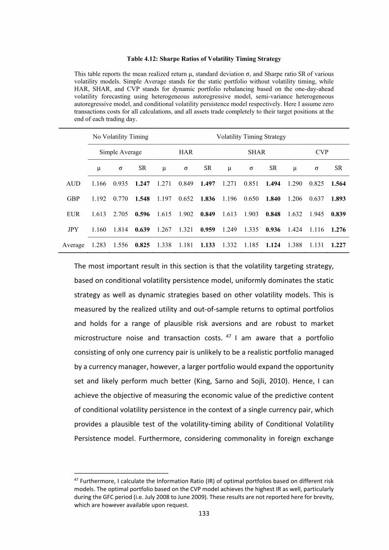
133

Table 4.12: Sharpe Ratios of Volatility Timing Strategy

This table reports the mean realized return μ, standard deviation σ, and Sharpe ratio SR of various

volatility models. Simple Average stands for the static portfolio without volatility timing, while

HAR, SHAR, and CVP stands for dynamic portfolio rebalancing based on the one-day-ahead

volatility forecasting using heterogeneous autoregressive model, semi-variance heterogeneous

autoregressive model, and conditional volatility persistence model respectively. Here I assume zero

transactions costs for all calculations, and all assets trade completely to their target positions at the

end of each trading day.

No Volatility Timing Volatility Timing Strategy

Simple Average HAR SHAR CVP

μ σ SR μ σ SR μ σ SR μ σ SR

AUD 1.166 0.935 1.247 1.271 0.849 1.497 1.271 0.851 1.494 1.290 0.825 1.564

GBP 1.192 0.770 1.548 1.197 0.652 1.836 1.196 0.650 1.840 1.206 0.637 1.893

EUR 1.613 2.705 0.596 1.615 1.902 0.849 1.613 1.903 0.848 1.632 1.945 0.839

JPY 1.160 1.814 0.639 1.267 1.321 0.959 1.249 1.335 0.936 1.424 1.116 1.276

Average 1.283 1.556 0.825 1.338 1.181 1.133 1.332 1.185 1.124 1.388 1.131 1.227

The most important result in this section is that the volatility targeting strategy,

based on conditional volatility persistence model, uniformly dominates the static

strategy as well as dynamic strategies based on other volatility models. This is

measured by the realized utility and out-of-sample returns to optimal portfolios

and holds for a range of plausible risk aversions and are robust to market

microstructure noise and transaction costs. 47 I am aware that a portfolio

consisting of only one currency pair is unlikely to be a realistic portfolio managed

by a currency manager, however, a larger portfolio would expand the opportunity

set and likely perform much better (King, Sarno and Sojli, 2010). Hence, I can

achieve the objective of measuring the economic value of the predictive content

of conditional volatility persistence in the context of a single currency pair, which

provides a plausible test of the volatility-timing ability of Conditional Volatility

Persistence model. Furthermore, considering commonality in foreign exchange

47 Furthermore, I calculate the Information Ratio (IR) of optimal portfolios based on different risk models. The optimal portfolio based on the CVP model achieves the highest IR as well, particularly during the GFC period (i.e. July 2008 to June 2009). These results are not reported here for brevity, which are however available upon request.

134

volatility and liquidity, the generality of these empirical results can be grounded

to a large extent.

4.5. Robustness Analysis

In this section, I conduct a robustness analysis to examine the relative

performance of the CVP model by using noise-robust realized variance measures

as suggested in Section 4.2.2. Namely, I re-estimate the variant HAR models and

compare their performances by using the Two-scale Realized Variance (TSRV)

estimator which proves to be an efficient and robust-sound realized variance

measure. Interestingly, the results of the forecasting comparisons (i.e., the values

of loss functions of QLIKE and LMSE) suggest that the CVP model can still generates

better forecasting performance when using noise-robust variance measures.48

Instead I report the realized utilities calculated when forecasting using TSRV as

shown in Table 4.13. Interestingly, the results of economic gains are comparable

to those calculated by using RV. Overall, I can conclude that the conditional

volatility persistence which links market state variables to future volatility is

helpful in explaining the asymmetry and long memory in volatility even after

controlling for market microstructure noise. The model which incorporates the

feature of conditional volatility persistence can outperform other dynamic

volatility models with regard to forecasting performance and economic value.

48 For the sake of brevity, I do not present those results, which are available upon request.

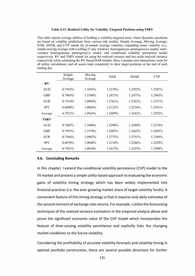
135

Table 4.13: Realized Utility for Volatility Targeted Positions using TSRV


are based on volatility predictions from various risk models. Simple Average, Moving Average,

HAR, SHAR, and CVP stands for in-sample average volatility, expanding mean volatility (i.e.,

simple moving average with a rolling 21-day window), heterogeneous autoregressive model, semi-

variance heterogeneous autoregressive model, and conditional volatility persistence model

respectively. RV and TSRV stands for using the realized variance and two-scale realized variance

respectively when estimating the RV-based HAR models. Here, I assume zero transactions costs for

all utility calculations, and all assets trade completely to their target positions at the end of each

trading day.

Simple

Average

Moving

Average HAR SHAR CVP

RV

AUD 0.7593% 1.1052% 1.2278% 1.2292% 1.2307%

GBP 0.7965% 1.1590% 1.2473% 1.2477% 1.2483%

EUR 0.7554% 1.0994% 1.2761% 1.2763% 1.3337%

JPY 0.6890% 1.0028% 1.2122% 1.2234% 1.2241%

Average 0.7521% 1.0916% 1.2409% 1.2442% 1.2592%

TSRV

AUD 0.7605% 1.1040% 1.2290% 1.2280% 1.2319%

GBP 0.7953% 1.1578% 1.2485% 1.2465% 1.2495%

EUR 0.7566% 1.0982% 1.2773% 1.2751% 1.3349%

JPY 0.6878% 1.0040% 1.2110% 1.2246% 1.2229%

Average 0.7501% 1.0910% 1.2415% 1.2435% 1.2598%

4.6. Concluding Remarks

In this chapter, I extend the conditional volatility persistence (CVP) model to the

FX market and present a simple utility-based approach to evaluating the economic

gains of volatility timing strategy which has been widely implemented into

financial practices (i.e. the ever-growing market share of target volatility funds). A

convenient feature of this timing strategy is that it requires only daily estimates of

the second moment of exchange rate returns. For example, I utilize the forecasting

techniques of the realized variance estimators in the empirical analysis above and

prove the significant economic value of the CVP model which incorporates the

feature of time-varying volatility persistence and explicitly links the changing

market conditions to the future volatility.

Considering the profitability of accurate volatility forecasts and volatility timing in

optimal portfolio construction, there are several possible directions for further

136

study. Firstly, it would be interesting to investigate whether more sophisticated

estimation techniques can lead to significant benefits, such as increased economic

gains of volatility forecasting; secondly, all of the forecasting models implemented

in this chapter are univariate. However, most practical questions related to risk

measurement and management are intrinsically multivariate in nature, requiring

the forecasts of both asset return variances and covariances. Whether the CVP

model can be applied to the portfolio construction in the multivariate context

deserves further study.

137

Chapter 5: Conclusions

This dissertation consists of three independent essays that explore different

aspects of price discovery and volatility dynamics in the FX market. The main

findings of each chapter can be summarised as follows:

I estimate the magnitudes and determinants of global information distribution of

AUD trading in the Asian, European, and North American markets in the second

chapter. Specifically, using the firm quotes of AUD against the US dollar from

January 1999 to December 2013, and employing a non-parametric methodology

of price discovery measures, i.e., the Two-scale Realized Variance (TSRV) ratio, I

estimate the information shares of global AUD trading. I find that the European

market and US market, particularly the overlapping trading session of London and

New York, dominate the price discovery process in AUD market, but Asia is rapidly

gaining information shares even with its declining market share of daily

transactions. After estimating the information shares, I focus on the short- and

long-run determinants in each market. The empirical analysis shows that after

controlling for spillover effects and dynamic natures of information shares, more

favourable market states and more unexpected order flows on macroeconomic

announcement days make a significantly positive contribution to price discovery

for AUD trading in the short-run, while a higher degree of market integration and

capital market openness, as proxied by the Chinn-Ito Index, contributes to price

discovery in the long-run.

In the third chapter, I revisit the meteor showers and heat waves effects for

AUD/USD, GBP/USD, EUR/USD, and USD/JPY spanning from January 1999 (January

2000 for EUR) to December 2013. Utilizing the volatility measures based on high-

frequency data, I find evidence of both meteor showers and heat waves effects in

the four trading segments of global FX market, which is consistent with Lahaye and

Neely (2016) who divide a calendar day into five segments and confirm the

presence of meteor shower and heat waves effect in each segment. However,

unlike Lahaye and Neely (2016), I find that the relative importance of meteor

138

shower effect has been increasing rapidly and has predominated over heat waves

effects in the intra-daily volatility spillovers, which emphasizes the increasing

interdependence and interconnectedness in the global FX market. By investigating

the patterns and economic mechanisms of meteor showers and heat waves

effects, I contribute to the literature regarding volatility spillover in the financial

markets. Specifically, I identify the key factors causing volatility spillovers in

different trading sessions, which highlight the complex geographical nature of the

FX market. Namely, the conditional volatility persistence is the fundamental

channel linking each region’s market states to the future volatility. These empirical

results argue in favour of modelling FX volatility dynamics segment-wise, rather

than in the more traditional approach of assuming a homogeneous process.

In the fourth chapter, I comprehensively investigate the role of conditional

volatility persistence in predicting future volatility from both statistical and

economic perspectives. I show that taking into account conditional volatility

persistence improves volatility forecasts both in-sample and out-of-sample. For

example, by utilizing the Shapley decomposition techniques, I find that the

conditional volatility persistence explains large portions of the variations in future

volatility and is the dominant channel linking market states to future volatility.

Moreover, I show that these statistical improvements can be translated into

economic values. By developing a simple yet accurate utility framework based on

mean-variance analysis, I show that under empirically realistic assumptions, the

CVP model is worth at least 0.51% of wealth per year relative to a static risk model,

and can achieve higher Sharpe ratios, particularly during the turmoil period. The

results hold true across the major exchange rates and are robust to market

microstructure effects and transaction costs.

In sum, the empirical findings presented in this dissertation provide a thorough

analysis of the information distribution and propagation in one of the largest

financial markets – the Foreign Exchange (FX) market. The empirical studies

discussed in this thesis also deepen our understanding of the microstructure of

the FX market. Besides, the evidence presented in this thesis could be of great

interest to academics, practitioners, and regulators, and can potentially aid policy

139

development of the FX market which remains opaque to a great extent (Rime and

Schrimpf, 2013). The empirical evidences presented in this dissertation will

provide important policy implications, especially for emerging markets, which are

still in the process of currency internationalization. For example, with the

increasing interdependence and interconnectedness in the global FX market, the

authorities in emerging markets have to strike a balance between maintaining

exchange rate stability and internationalizing their currency in the face of growing

international capital flows.

There are several possible directions for further study. For example, how to

accurately measure the price discovery in the financial markets is one question

that is yet to be fully answered and better understood. Furthermore, additional

research is required to consider the generalizability of these results. This will

involve considering price discovery and volatility dynamics in other major

currencies, as well as in emerging market currencies. Besides, how to identify the

institutional sources of long-memory in volatility and its spillovers deserves further

study, which will definitely improve our understanding of volatility transmission

and extend our economic intuition of risk contagion in the financial markets.

Another possible direction is to assess the economic values of volatility timing in

more concrete financial applications such as multi-period portfolio management

in the multivariate context as in Fleming et al. (2001, 2003). Lastly, the intraday

relationship between markets can be affected by microstructure differences such

as institutional features, heterogeneous investors, or different trading rules.

Therefore, more investigation on the effects of microstructure over volatility

dynamics mechanisms would be highly desirable.

140

Appendices

Appendix A: Turnover of foreign exchange instruments, by currency

This table reports the average daily turnover of top-5 most traded currencies from April 2010 to

April 2016. It is based on the triennial central bank surveys conducted by the Bank for International

Settlements (BIS, 2010, 2013, and 2016). Amount includes spot, outright forward, and swap

transactions which is measured in billions of USD and percentage share. The percentage shares sum

to 200% because two currencies are involved in each transaction.

2010 2013 2016

Amount Percent Amount Percent Amount Percent

USD 3,371 84.91 4,662 87.02 4,438 87.26

EUR 1,551 39.02 1,790 33.43 1,591 31.43

JPY 754 19.01 1,235 23.06 1,096 21.65

GBP 512 12.94 633 11.86 649 12.86

AUD 301 7.63 463 8.62 348 6.92

Global

Total 3,973 200.00 5,357 200.00 5,067 200.00

Appendix B: Average daily transactions of AUD

This table reports the average daily transactions for AUD against USD from April 2007 to April

2013 in the top-10 foreign exchange markets. It is based on a series of triennial central bank surveys

conducted by the Bank for International Settlements (BIS, 2007, 2010, and 2013). Volumes include

spot, outright forward, and swap transactions and are measured in billion USD.

AUD 2007 2010 2013

Value Precent Value Precent Value Precent

Australia 76.70 33.41 75.50 23.09 80.50 17.30

Denmark 0.46 0.20 1.40 0.43 2.31 0.50

France 5.89 2.57 6.25 1.91 9.00 1.93

Germany 1.25 0.54 2.11 0.65 3.08 0.66

Hong Kong 14.00 6.10 24.64 7.54 20.81 4.47

Japan 10.60 4.62 8.16 2.50 18.11 3.89

Singapore 15.70 6.84 27.57 8.43 37.19 7.99

Switzerland 6.12 2.67 10.08 3.08 8.12 1.75

United Kingdom 55.90 24.35 102.00 31.19 181.80 39.08

United States 30.90 13.46 56.06 17.14 82.39 17.71

Asia in Top 10 117.00 50.96 135.87 41.55 156.61 33.67

Europe in Top 10 69.60 30.31 121.84 37.26 204.31 43.92

America in Top 10 30.90 13.46 56.06 17.14 82.39 17.71

Top 10 217.50 94.73 313.77 95.95 443.31 95.29

Global Total 229.60 100.00 327.00 100.00 465.20 100.00

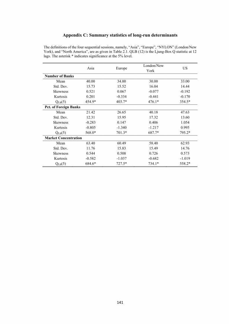
141

Appendix C: Summary statistics of long-run determinants

The definitions of the four sequential sessions, namely, “Asia”, “Europe”, “NYLON” (London/New

York), and “North America”, are as given in Table 2.1. QLB (12) is the Ljung-Box Q statistic at 12

lags. The asterisk * indicates significance at the 5% level.


York US

Number of Banks

Mean 40.00 34.00 30.00 33.00

Std. Dev. 15.73 15.52 16.04 14.44

Skewness 0.521 0.067 -0.077 -0.192

Kurtosis 0.201 -0.334 -0.441 -0.170

QLB(5) 454.9* 403.7* 476.1* 354.5*

Pct. of Foreign Banks

Mean 21.42 26.65 40.18 47.63

Std. Dev. 12.31 15.95 17.32 13.60

Skewness -0.283 0.147 0.406 1.054

Kurtosis -0.805 -1.340 -1.217 0.995

QLB(5) 568.0* 701.3* 687.7* 795.2*

Market Concentration

Mean 63.40 60.49 58.40 62.93

Std. Dev. 11.76 15.83 15.49 14.76

Skewness 0.544 0.508 0.726 0.573

Kurtosis -0.582 -1.037 -0.682 -1.019

QLB(5) 684.6* 727.5* 734.1* 558.2*

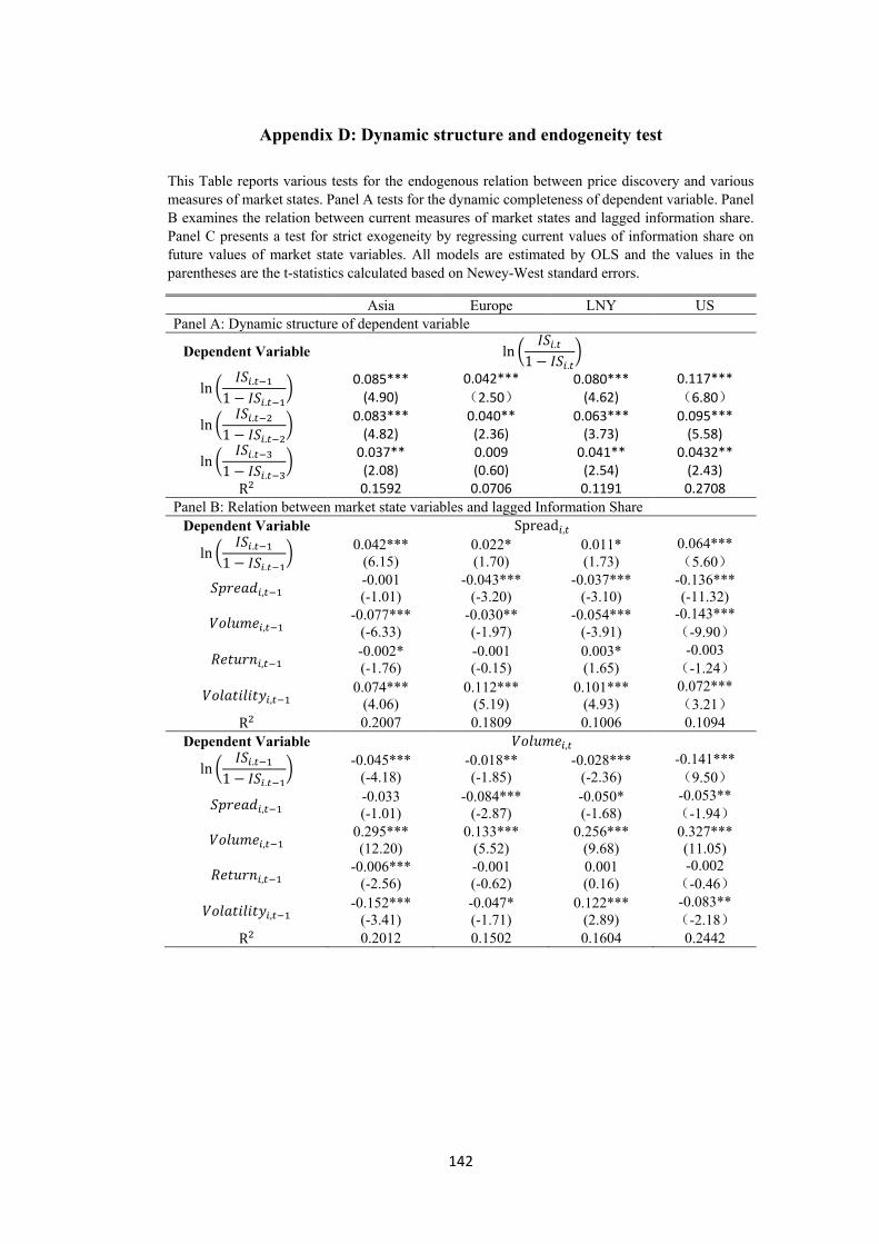
142

Appendix D: Dynamic structure and endogeneity test

This Table reports various tests for the endogenous relation between price discovery and various

measures of market states. Panel A tests for the dynamic completeness of dependent variable. Panel

B examines the relation between current measures of market states and lagged information share.

Panel C presents a test for strict exogeneity by regressing current values of information share on

future values of market state variables. All models are estimated by OLS and the values in the

parentheses are the t-statistics calculated based on Newey-West standard errors.

Asia Europe LNY US

Panel A: Dynamic structure of dependent variable

Dependent Variable ln (𝐼𝑆𝑖.𝑡

1 − 𝐼𝑆𝑖.𝑡)


1 − 𝐼𝑆𝑖.𝑡−1)

0.085*** (4.90)

0.042***

（2.50）

0.080*** (4.62)

0.117***

（6.80）


1 − 𝐼𝑆𝑖.𝑡−2)

0.083*** (4.82)

0.040** (2.36)

0.063*** (3.73)

0.095*** (5.58)


1 − 𝐼𝑆𝑖.𝑡−3)

0.037** (2.08)

0.009 (0.60)

0.041** (2.54)

0.0432** (2.43)

R2 0.1592 0.0706 0.1191 0.2708

Panel B: Relation between market state variables and lagged Information Share

Dependent Variable Spread𝑖,𝑡


1 − 𝐼𝑆𝑖.𝑡−1)

0.042***

(6.15)

0.022*

(1.70)

0.011*

(1.73)

0.064***

（5.60）

𝑆𝑝𝑟𝑒𝑎𝑑𝑖,𝑡−1 -0.001

(-1.01)

-0.043***

(-3.20)

-0.037***

(-3.10)

-0.136***

(-11.32)

𝑉𝑜𝑙𝑢𝑚𝑒𝑖,𝑡−1 -0.077***

(-6.33)

-0.030**

(-1.97)

-0.054***

(-3.91)

-0.143***

（-9.90）

𝑅𝑒𝑡𝑢𝑟𝑛𝑖,𝑡−1 -0.002*

(-1.76)

-0.001

(-0.15)

0.003*

(1.65)

-0.003

（-1.24）

𝑉𝑜𝑙𝑎𝑡𝑖𝑙𝑖𝑡𝑦𝑖,𝑡−1 0.074***

(4.06)

0.112***

(5.19)

0.101***

(4.93)

0.072***

（3.21）

R2 0.2007 0.1809 0.1006 0.1094

Dependent Variable 𝑉𝑜𝑙𝑢𝑚𝑒𝑖,𝑡


1 − 𝐼𝑆𝑖.𝑡−1)

-0.045***

(-4.18)

-0.018**

(-1.85)

-0.028***

(-2.36)

-0.141***

（9.50）

𝑆𝑝𝑟𝑒𝑎𝑑𝑖,𝑡−1 -0.033

(-1.01)

-0.084***

(-2.87)

-0.050*

(-1.68)

-0.053**

（-1.94）

𝑉𝑜𝑙𝑢𝑚𝑒𝑖,𝑡−1 0.295***

(12.20)

0.133***

(5.52)

0.256***

(9.68)

0.327***

(11.05)

𝑅𝑒𝑡𝑢𝑟𝑛𝑖,𝑡−1 -0.006***

(-2.56)

-0.001

(-0.62)

0.001

(0.16)

-0.002

（-0.46）

𝑉𝑜𝑙𝑎𝑡𝑖𝑙𝑖𝑡𝑦𝑖,𝑡−1 -0.152***

(-3.41)

-0.047*

(-1.71)

0.122***

(2.89)

-0.083**

（-2.18）

R2 0.2012 0.1502 0.1604 0.2442

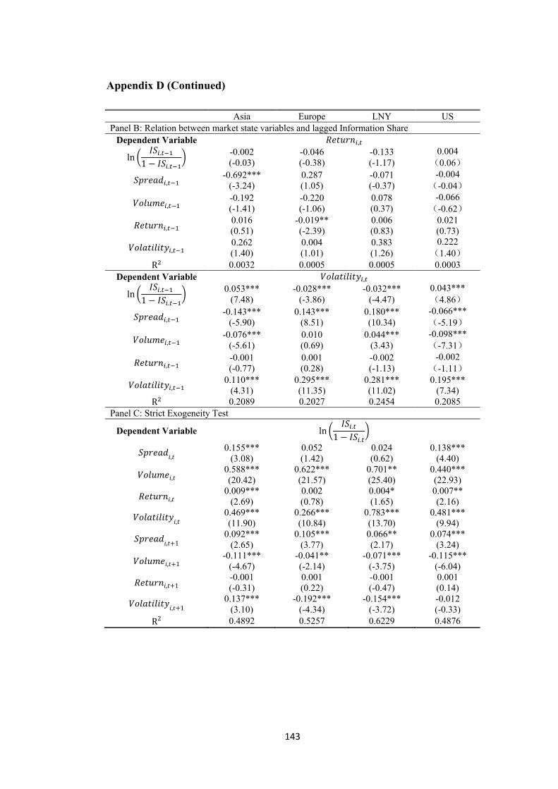
143

Appendix D (Continued)

Asia Europe LNY US

Panel B: Relation between market state variables and lagged Information Share

Dependent Variable 𝑅𝑒𝑡𝑢𝑟𝑛𝑖,𝑡


1 − 𝐼𝑆𝑖.𝑡−1)

-0.002

(-0.03)

-0.046

(-0.38)

-0.133

(-1.17)

0.004

（0.06）

𝑆𝑝𝑟𝑒𝑎𝑑𝑖,𝑡−1 -0.692***

(-3.24)

0.287

(1.05)

-0.071

(-0.37)

-0.004

（-0.04）

𝑉𝑜𝑙𝑢𝑚𝑒𝑖,𝑡−1 -0.192

(-1.41)

-0.220

(-1.06)

0.078

(0.37)

-0.066

（-0.62）

𝑅𝑒𝑡𝑢𝑟𝑛𝑖,𝑡−1 0.016

(0.51)

-0.019**

(-2.39)

0.006

(0.83)

0.021

(0.73)

𝑉𝑜𝑙𝑎𝑡𝑖𝑙𝑖𝑡𝑦𝑖,𝑡−1 0.262

(1.40)

0.004

(1.01)

0.383

(1.26)

0.222

（1.40）

R2 0.0032 0.0005 0.0005 0.0003

Dependent Variable 𝑉𝑜𝑙𝑎𝑡𝑖𝑙𝑖𝑡𝑦𝑖,𝑡


1 − 𝐼𝑆𝑖.𝑡−1)

0.053***

(7.48)

-0.028***

(-3.86)

-0.032***

(-4.47)

0.043***

（4.86）

𝑆𝑝𝑟𝑒𝑎𝑑𝑖,𝑡−1 -0.143***

(-5.90)

0.143***

(8.51)

0.180***

(10.34)

-0.066***

（-5.19）

𝑉𝑜𝑙𝑢𝑚𝑒𝑖,𝑡−1 -0.076***

(-5.61)

0.010

(0.69)

0.044***

(3.43)

-0.098***

（-7.31）

𝑅𝑒𝑡𝑢𝑟𝑛𝑖,𝑡−1 -0.001

(-0.77)

0.001

(0.28)

-0.002

(-1.13)

-0.002

（-1.11）

𝑉𝑜𝑙𝑎𝑡𝑖𝑙𝑖𝑡𝑦𝑖,𝑡−1 0.110***

(4.31)

0.295***

(11.35)

0.281***

(11.02)

0.195***

(7.34)

R2 0.2089 0.2027 0.2454 0.2085

Panel C: Strict Exogeneity Test

Dependent Variable ln (𝐼𝑆𝑖.𝑡

1 − 𝐼𝑆𝑖.𝑡)

𝑆𝑝𝑟𝑒𝑎𝑑𝑖,𝑡

0.155***

(3.08)

0.052

(1.42)

0.024

(0.62)

0.138***

(4.40)

𝑉𝑜𝑙𝑢𝑚𝑒𝑖,𝑡 0.588***

(20.42)

0.622***

(21.57)

0.701**

(25.40)

0.440***

(22.93)

𝑅𝑒𝑡𝑢𝑟𝑛𝑖,𝑡 0.009***

(2.69)

0.002

(0.78)

0.004*

(1.65)

0.007**

(2.16)

𝑉𝑜𝑙𝑎𝑡𝑖𝑙𝑖𝑡𝑦𝑖,𝑡

0.469***

(11.90)

0.266***

(10.84)

0.783***

(13.70)

0.481***

(9.94)

𝑆𝑝𝑟𝑒𝑎𝑑𝑖,𝑡+1

0.092***

(2.65)

0.105***

(3.77)

0.066**

(2.17)

0.074***

(3.24)

𝑉𝑜𝑙𝑢𝑚𝑒𝑖,𝑡+1 -0.111***

(-4.67)

-0.041**

(-2.14)

-0.071***

(-3.75)

-0.115***

(-6.04)

𝑅𝑒𝑡𝑢𝑟𝑛𝑖,𝑡+1 -0.001

(-0.31)

0.001

(0.22)

-0.001

(-0.47)

0.001

(0.14)

𝑉𝑜𝑙𝑎𝑡𝑖𝑙𝑖𝑡𝑦𝑖,𝑡+1

0.137***

(3.10)

-0.192***

(-4.34)

-0.154***

(-3.72)

-0.012

(-0.33)

R2 0.4892 0.5257 0.6229 0.4876

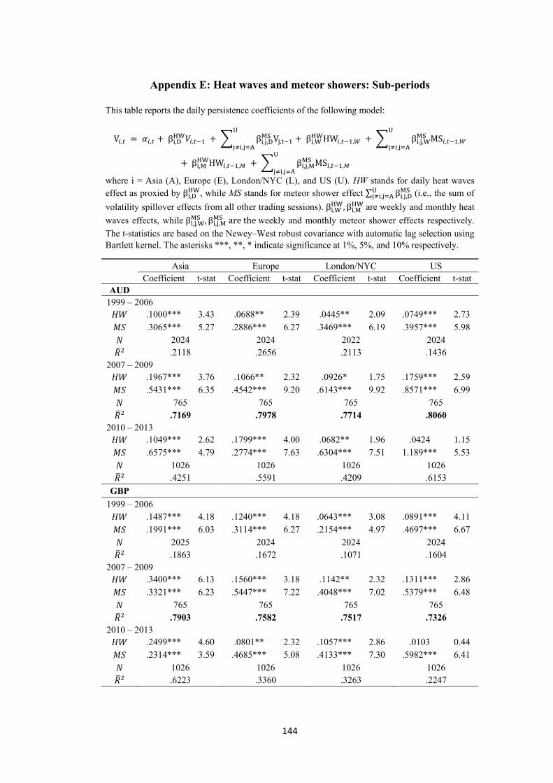
144

Appendix E: Heat waves and meteor showers: Sub-periods



MS Vj,t−1

U

j≠i,j=A+ βi,W

HWHW𝑖,𝑡−1,𝑊 + ∑ βi,j,WMS MS𝑖,𝑡−1,𝑊

U

j≠i,j=A



U

j≠i,j=A

where i = Asia (A), Europe (E), London/NYC (L), and US (U). HW stands for daily heat waves

effect as proxied by βi,DHW, while MS stands for meteor shower effect ∑ βi,j,D

MSUj≠i,j=A (i.e., the sum of

volatility spillover effects from all other trading sessions). βi,WHW, βi,M

HW are weekly and monthly heat

waves effects, while βi,j,WMS , βi,j,M

MS are the weekly and monthly meteor shower effects respectively.

The t-statistics are based on the Newey–West robust covariance with automatic lag selection using

Bartlett kernel. The asterisks ***, **, * indicate significance at 1%, 5%, and 10% respectively.



AUD

1999 – 2006

𝐻𝑊 .1000*** 3.43 .0688** 2.39 .0445** 2.09 .0749*** 2.73

𝑀𝑆 .3065*** 5.27 .2886*** 6.27 .3469*** 6.19 .3957*** 5.98

𝑁 2024 2024 2022 2024

�̅�2 .2118 .2656 .2113 .1436

2007 – 2009

𝐻𝑊 .1967*** 3.76 .1066** 2.32 .0926* 1.75 .1759*** 2.59

𝑀𝑆 .5431*** 6.35 .4542*** 9.20 .6143*** 9.92 .8571*** 6.99

𝑁 765 765 765 765

�̅�2 .7169 .7978 .7714 .8060

2010 – 2013

𝐻𝑊 .1049*** 2.62 .1799*** 4.00 .0682** 1.96 .0424 1.15

𝑀𝑆 .6575*** 4.79 .2774*** 7.63 .6304*** 7.51 1.189*** 5.53

𝑁 1026 1026 1026 1026

�̅�2 .4251 .5591 .4209 .6153

GBP

1999 – 2006

𝐻𝑊 .1487*** 4.18 .1240*** 4.18 .0643*** 3.08 .0891*** 4.11

𝑀𝑆 .1991*** 6.03 .3114*** 6.27 .2154*** 4.97 .4697*** 6.67

𝑁 2025 2024 2024 2024

�̅�2 .1863 .1672 .1071 .1604

2007 – 2009

𝐻𝑊 .3400*** 6.13 .1560*** 3.18 .1142** 2.32 .1311*** 2.86

𝑀𝑆 .3321*** 6.23 .5447*** 7.22 .4048*** 7.02 .5379*** 6.48

𝑁 765 765 765 765

�̅�2 .7903 .7582 .7517 .7326

2010 – 2013

𝐻𝑊 .2499*** 4.60 .0801** 2.32 .1057*** 2.86 .0103 0.44

𝑀𝑆 .2314*** 3.59 .4685*** 5.08 .4133*** 7.30 .5982*** 6.41

𝑁 1026 1026 1026 1026

�̅�2 .6223 .3360 .3263 .2247

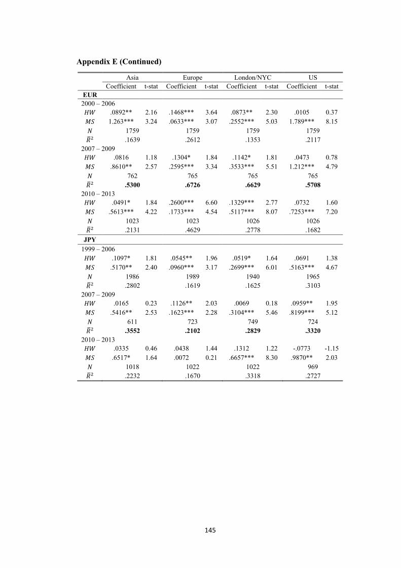
145

Appendix E (Continued)



EUR

2000 – 2006

𝐻𝑊 .0892** 2.16 .1468*** 3.64 .0873** 2.30 .0105 0.37

𝑀𝑆 1.263*** 3.24 .0633*** 3.07 .2552*** 5.03 1.789*** 8.15

𝑁 1759 1759 1759 1759

�̅�2 .1639 .2612 .1353 .2117

2007 – 2009

𝐻𝑊 .0816 1.18 .1304* 1.84 .1142* 1.81 .0473 0.78

𝑀𝑆 .8610** 2.57 .2595*** 3.34 .3533*** 5.51 1.212*** 4.79

𝑁 762 765 765 765

�̅�2 .5300 .6726 .6629 .5708

2010 – 2013

𝐻𝑊 .0491* 1.84 .2600*** 6.60 .1329*** 2.77 .0732 1.60

𝑀𝑆 .5613*** 4.22 .1733*** 4.54 .5117*** 8.07 .7253*** 7.20

𝑁 1023 1023 1026 1026

�̅�2 .2131 .4629 .2778 .1682

JPY

1999 – 2006

𝐻𝑊 .1097* 1.81 .0545** 1.96 .0519* 1.64 .0691 1.38

𝑀𝑆 .5170** 2.40 .0960*** 3.17 .2699*** 6.01 .5163*** 4.67

𝑁 1986 1989 1940 1965

�̅�2 .2802 .1619 .1625 .3103

2007 – 2009

𝐻𝑊 .0165 0.23 .1126** 2.03 .0069 0.18 .0959** 1.95

𝑀𝑆 .5416** 2.53 .1623*** 2.28 .3104*** 5.46 .8199*** 5.12

𝑁 611 723 749 724

�̅�2 .3552 .2102 .2829 .3320

2010 – 2013

𝐻𝑊 .0335 0.46 .0438 1.44 .1312 1.22 -.0773 -1.15

𝑀𝑆 .6517* 1.64 .0072 0.21 .6657*** 8.30 .9870** 2.03

𝑁 1018 1022 1022 969

�̅�2 .2232 .1670 .3318 .2727

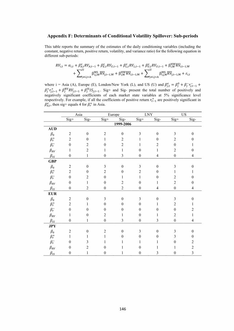
146

Appendix F: Determinants of Conditional Volatility Spillover: Sub-periods

This table reports the summary of the estimates of the daily conditioning variables (including the

constant, negative return, positive return, volatility, and variance ratio) for the following equation in

different sub-periods:




i,t−1,W


j,t−1,W

U

j≠i,j=A+ βi,M



U



0 + 𝛽𝑗−𝑟𝑗,𝑡−1

− +



IS𝐼𝑆𝑗,𝑡−1 . Sig+ and Sig- present the total number of positively and

negatively significant coefficients of each market state variables at 5% significance level

respectively. For example, if all the coefficients of positive return 𝑟𝑡−1+ are positively significant in

𝛽𝐴,𝑡𝑒 , then sig+ equals 4 for 𝛽𝑟

+ in Asia.

Asia Europe LNY US

Sig+ Sig- Sig+ Sig- Sig+ Sig- Sig+ Sig-

1999-2006

AUD

𝛽0 2 0 2 0 3 0 3 0

𝛽𝑟+ 2 0 1 2 1 0 2 0

𝛽𝑟− 0 2 0 2 1 2 0 1

𝛽𝑅𝑉 1 2 1 1 0 1 2 0

𝛽𝐼𝑆 0 1 0 3 0 4 0 4

GBP

𝛽0 2 0 3 0 3 0 3 0

𝛽𝑟+ 2 0 2 0 2 0 1 1

𝛽𝑟− 0 2 0 1 1 0 2 0

𝛽𝑅𝑉 0 1 0 2 0 1 2 0

𝛽𝐼𝑆 0 2 0 2 0 4 0 4

EUR

𝛽0 2 0 3 0 3 0 3 0

𝛽𝑟+ 2 1 0 0 0 1 2 1

𝛽𝑟− 0 0 0 0 0 0 0 2

𝛽𝑅𝑉 1 0 2 1 0 1 2 1

𝛽𝐼𝑆 0 1 0 3 0 3 0 4

JPY

𝛽0 2 0 2 0 3 0 3 0

𝛽𝑟+ 1 1 1 0 0 0 3 0

𝛽𝑟− 0 3 1 1 1 1 0 2

𝛽𝑅𝑉 0 2 0 1 0 1 1 2

𝛽𝐼𝑆 0 1 0 1 0 3 0 3

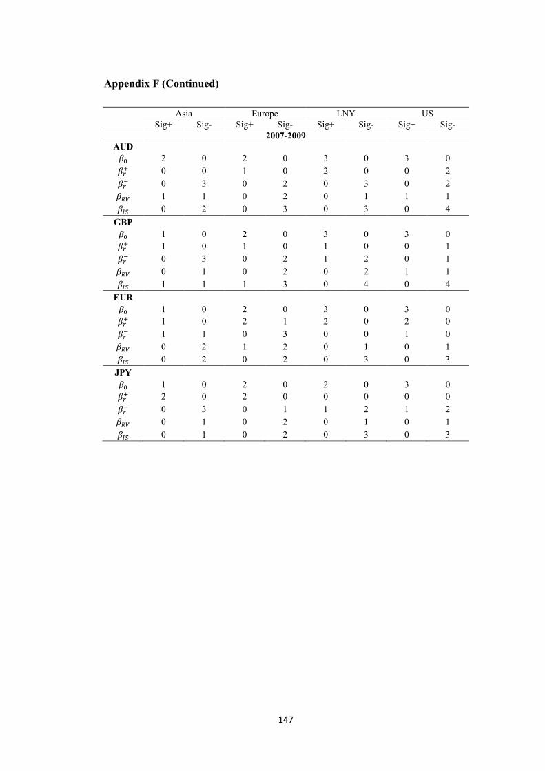
147

Appendix F (Continued)

Asia Europe LNY US


2007-2009

AUD

𝛽0 2 0 2 0 3 0 3 0

𝛽𝑟+ 0 0 1 0 2 0 0 2

𝛽𝑟− 0 3 0 2 0 3 0 2

𝛽𝑅𝑉 1 1 0 2 0 1 1 1

𝛽𝐼𝑆 0 2 0 3 0 3 0 4

GBP

𝛽0 1 0 2 0 3 0 3 0

𝛽𝑟+ 1 0 1 0 1 0 0 1

𝛽𝑟− 0 3 0 2 1 2 0 1

𝛽𝑅𝑉 0 1 0 2 0 2 1 1

𝛽𝐼𝑆 1 1 1 3 0 4 0 4

EUR

𝛽0 1 0 2 0 3 0 3 0

𝛽𝑟+ 1 0 2 1 2 0 2 0

𝛽𝑟− 1 1 0 3 0 0 1 0

𝛽𝑅𝑉 0 2 1 2 0 1 0 1

𝛽𝐼𝑆 0 2 0 2 0 3 0 3

JPY

𝛽0 1 0 2 0 2 0 3 0

𝛽𝑟+ 2 0 2 0 0 0 0 0

𝛽𝑟− 0 3 0 1 1 2 1 2

𝛽𝑅𝑉 0 1 0 2 0 1 0 1

𝛽𝐼𝑆 0 1 0 2 0 3 0 3

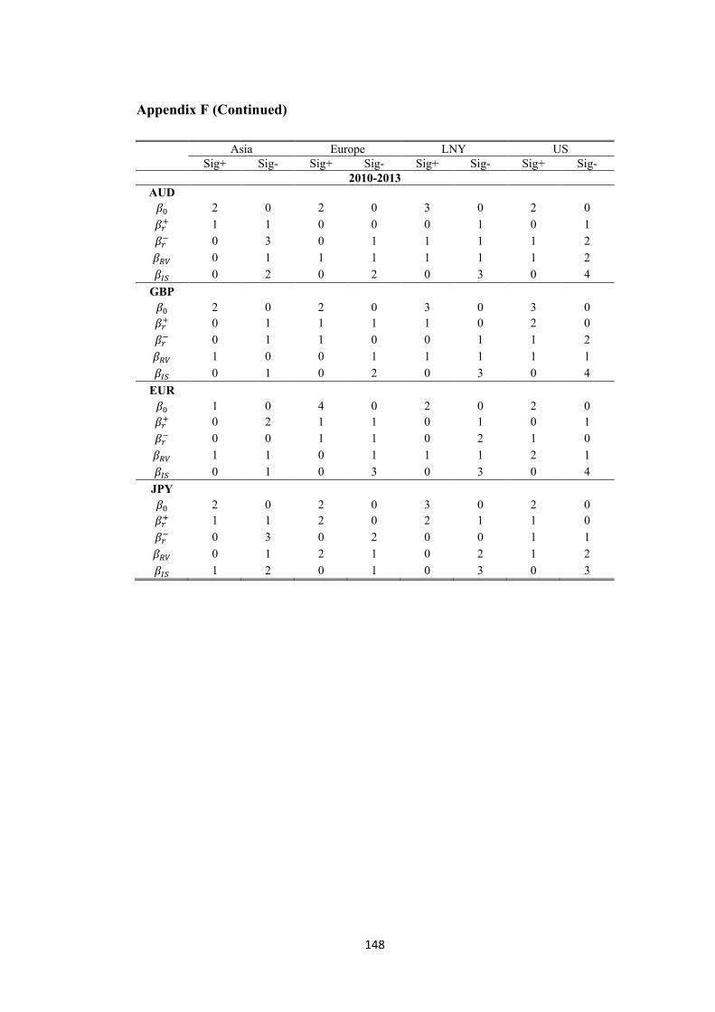
148

Appendix F (Continued)

Asia Europe LNY US


2010-2013

AUD

𝛽0 2 0 2 0 3 0 2 0

𝛽𝑟+ 1 1 0 0 0 1 0 1

𝛽𝑟− 0 3 0 1 1 1 1 2

𝛽𝑅𝑉 0 1 1 1 1 1 1 2

𝛽𝐼𝑆 0 2 0 2 0 3 0 4

GBP

𝛽0 2 0 2 0 3 0 3 0

𝛽𝑟+ 0 1 1 1 1 0 2 0

𝛽𝑟− 0 1 1 0 0 1 1 2

𝛽𝑅𝑉 1 0 0 1 1 1 1 1

𝛽𝐼𝑆 0 1 0 2 0 3 0 4

EUR

𝛽0 1 0 4 0 2 0 2 0

𝛽𝑟+ 0 2 1 1 0 1 0 1

𝛽𝑟− 0 0 1 1 0 2 1 0

𝛽𝑅𝑉 1 1 0 1 1 1 2 1

𝛽𝐼𝑆 0 1 0 3 0 3 0 4

JPY

𝛽0 2 0 2 0 3 0 2 0

𝛽𝑟+ 1 1 2 0 2 1 1 0

𝛽𝑟− 0 3 0 2 0 0 1 1

𝛽𝑅𝑉 0 1 2 1 0 2 1 2

𝛽𝐼𝑆 1 2 0 1 0 3 0 3

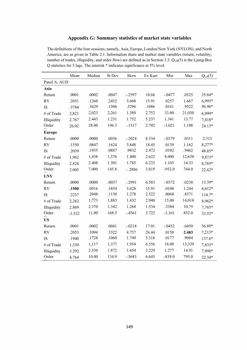
149

Appendix G: Summary statistics of market state variables

The definitions of the four sessions, namely, Asia, Europe, London/New York (NYLON), and North

America, are as given in Table 2.1. Information share and market state variables (return, volatility,

number of trades, illiquidity, and order flow) are defined as in Section 3.3. QLB(5) is the Ljung-Box

Q statistics for 5 lags. The asterisk * indicates significance at 5% level.

Mean Median St Dev Skew Ex Kurt Min Max QLB(5)

Panel A: AUD

Asia

Return .0001 .0002 .0047 -.2597 10.66 -.0477 .0525 35.64*

RV .2051 .1260 .2452 3.608 15.91 .0257 1.667 6,993*

IS .3784 .3629 .1506 .5296 .1086 .0161 .9522 96.96*

# of Trade 2,821 2,023 2,261 1.389 2.752 33.00 21,030 6,999*

Illiquidity 2.767 2.443 1.231 1.752 5.237 1.341 13.77 7,818*

Order

Flow 26.02 28.00 196.3 -.1517 2.702 -1,021 1,108 24.13*

Europe

Return .0000 .0000 .0036 -.2024 8.534 -.0379 .0311 2.315

RV .1350 .0847 .1624 3.848 18.45 .0139 1.162 8,277*

IS .2039 .1935 .0887 .9832 2.472 .0102 .9462 48.85*

# of Trade 1,962 1,438 1,576 1.400 2.622 8.000 12,638 9,873*

Illiquidity 2.828 2.408 1.301 1.785 6.233 1.103 14.33 8,765*

Order

Flow 2.005 7.000 145.8 -.2886 3.819 -952.0 744.0 22.62*

LNY

Return .0000 .0000 .0037 -.2991 6.583 -.0372 .0238 13.39*

RV .1500 .0916 .1854 3.628 15.91 .0108 1.244 6,612*

IS .2237 .2048 .1130 1.278 2.522 .0068 .8371 114.7*

# of Trade 2,282 1,773 1,883 1.432 2.940 15.00 14,018 8,962*

Illiquidity 2.869 2.370 1.342 1.268 1.534 .3384 10.75 7,765*

Order

Flow -1.522 11.00 168.5 -.4561 3.722 -1,161 852.0 32.52*

US

Return .0001 .0002 .0041 -.0218 17.01 -.0452 .0450 36.89*

RV .2053 .1094 .3322 4.757 26.44 .0158 2.483 7,213*

IS .1940 .1728 .1060 1.749 5.318 .0177 .9084 137.6*

# of Trade 1,530 1,117 1,377 1.954 6.556 18.00 13,339 7,833*

Illiquidity 3.292 2.530 1.872 1.454 2.229 1.277 14.91 7,998*

Order

Flow 4.764 10.00 134.9 -.5683 6.645 -839.0 795.0 22.34*

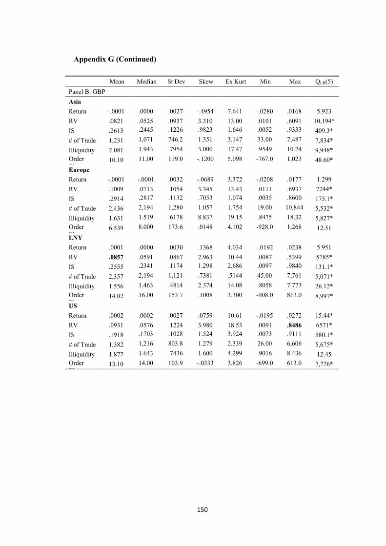
150

Appendix G (Continued)


Panel B: GBP

Asia

Return -.0001 .0000 .0027 -.4954 7.641 -.0280 .0168 5.923

RV .0821 .0525 .0937 3.310 13.00 .0101 .6091 10,194*

IS .2613 .2445 .1226 .9823 1.646 .0052 .9333 409.3*

# of Trade 1,231 1,071 746.2 1.351 3.147 33.00 7,487 7,834*

Illiquidity 2.081 1.943 .7954 3.000 17.47 .9549 10.24 9,948*

Order

Flow 10.10 11.00 119.0 -.1200 5.098 -767.0 1,023 48.60*

Europe

Return -.0001 -.0001 .0032 -.0689 3.372 -.0208 .0177 1.299

RV .1009 .0713 .1054 3.345 13.43 .0111 .6937 7244*

IS .2914 .2817 .1132 .7053 1.074 .0035 .8600 175.1*

# of Trade 2,436 2,194 1,280 1.057 1.754 19.00 10,844 5,532*

Illiquidity 1.631 1.519 .6178 8.837 19.15 .8475 18.32 5,827*

Order

Flow 6.539 8.000 173.6 .0148 4.102 -928.0 1,268 12.51

LNY

Return .0001 .0000 .0030 .1368 4.034 -.0192 .0238 5.951

RV .0857 .0591 .0867 2.963 10.44 .0087 .5399 5785*

IS .2555 .2341 .1174 1.298 2.686 .0097 .9840 131.1*

# of Trade 2,357 2,194 1,121 .7381 .5144 45.00 7,761 5,071*

Illiquidity 1.556 1.463 .4814 2.374 14.08 .8058 7.773 26.12*

Order

Flow 14.02 16.00 153.7 .1008 3.300 -908.0 813.0 8,997*

US

Return .0002 .0002 .0027 .0759 10.61 -.0195 .0272 15.44*

RV .0931 .0576 .1224 3.980 18.53 .0091 .8486 6571*

IS .1918 .1703 .1028 1.524 3.924 .0073 .9111 580.1*

# of Trade 1,382 1,216 803.8 1.279 2.339 26.00 6,606 5,675*

Illiquidity 1.877 1.643 .7436 1.600 4.299 .9016 8.436 12.45

Order

Flow 13.10 14.00 103.9 -.0333 3.826 -699.0 613.0 7,776*

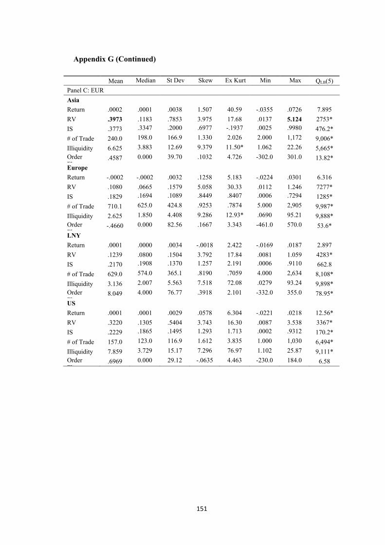
151



Panel C: EUR

Asia

Return .0002 .0001 .0038 1.507 40.59 -.0355 .0726 7.895

RV .3973 .1183 .7853 3.975 17.68 .0137 5.124 2753*

IS .3773 .3347 .2000 .6977 -.1937 .0025 .9980 476.2*

# of Trade 240.0 198.0 166.9 1.330 2.026 2.000 1,172 9,006*

Illiquidity 6.625 3.883 12.69 9.379 11.50* 1.062 22.26 5,665*

Order

Flow .4587 0.000 39.70 .1032 4.726 -302.0 301.0 13.82*

Europe

Return -.0002 -.0002 .0032 .1258 5.183 -.0224 .0301 6.316

RV .1080 .0665 .1579 5.058 30.33 .0112 1.246 7277*

IS .1829 .1694 .1089 .8449 .8407 .0006 .7294 1285*

# of Trade 710.1 625.0 424.8 .9253 .7874 5.000 2,905 9,987*

Illiquidity 2.625 1.850 4.408 9.286 12.93* .0690 95.21 9,888*

Order

Flow -.4660 0.000 82.56 .1667 3.343 -461.0 570.0 53.6*

LNY

Return .0001 .0000 .0034 -.0018 2.422 -.0169 .0187 2.897

RV .1239 .0800 .1504 3.792 17.84 .0081 1.059 4283*

IS .2170 .1908 .1370 1.257 2.191 .0006 .9110 662.8

# of Trade 629.0 574.0 365.1 .8190 .7059 4.000 2,634 8,108*

Illiquidity 3.136 2.007 5.563 7.518 72.08 .0279 93.24 9,898*

Order

Flow 8.049 4.000 76.77 .3918 2.101 -332.0 355.0 78.95*

US

Return .0001 .0001 .0029 .0578 6.304 -.0221 .0218 12.56*

RV .3220 .1305 .5404 3.743 16.30 .0087 3.538 3367*

IS .2229 .1865 .1495 1.293 1.713 .0002 .9312 170.2*

# of Trade 157.0 123.0 116.9 1.612 3.835 1.000 1,030 6,494*

Illiquidity 7.859 3.729 15.17 7.296 76.97 1.102 25.87 9,111*

Order

Flow .6969 0.000 29.12 -.0635 4.463 -230.0 184.0 6.58

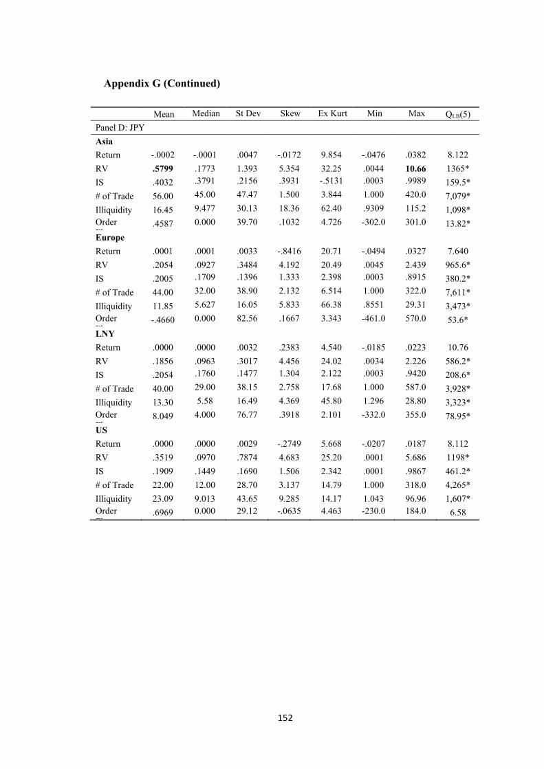
152



Panel D: JPY

Asia

Return -.0002 -.0001 .0047 -.0172 9.854 -.0476 .0382 8.122

RV .5799 .1773 1.393 5.354 32.25 .0044 10.66 1365*

IS .4032 .3791 .2156 .3931 -.5131 .0003 .9989 159.5*

# of Trade 56.00 45.00 47.47 1.500 3.844 1.000 420.0 7,079*

Illiquidity 16.45 9.477 30.13 18.36 62.40 .9309 115.2 1,098*

Order

Flow .4587 0.000 39.70 .1032 4.726 -302.0 301.0 13.82*

Europe

Return .0001 .0001 .0033 -.8416 20.71 -.0494 .0327 7.640

RV .2054 .0927 .3484 4.192 20.49 .0045 2.439 965.6*

IS .2005 .1709 .1396 1.333 2.398 .0003 .8915 380.2*

# of Trade 44.00 32.00 38.90 2.132 6.514 1.000 322.0 7,611*

Illiquidity 11.85 5.627 16.05 5.833 66.38 .8551 29.31 3,473*

Order

Flow -.4660 0.000 82.56 .1667 3.343 -461.0 570.0 53.6*

LNY

Return .0000 .0000 .0032 .2383 4.540 -.0185 .0223 10.76

RV .1856 .0963 .3017 4.456 24.02 .0034 2.226 586.2*

IS .2054 .1760 .1477 1.304 2.122 .0003 .9420 208.6*

# of Trade 40.00 29.00 38.15 2.758 17.68 1.000 587.0 3,928*

Illiquidity 13.30 5.58 16.49 4.369 45.80 1.296 28.80 3,323*

Order

Flow 8.049 4.000 76.77 .3918 2.101 -332.0 355.0 78.95*

US

Return .0000 .0000 .0029 -.2749 5.668 -.0207 .0187 8.112

RV .3519 .0970 .7874 4.683 25.20 .0001 5.686 1198*

IS .1909 .1449 .1690 1.506 2.342 .0001 .9867 461.2*

# of Trade 22.00 12.00 28.70 3.137 14.79 1.000 318.0 4,265*

Illiquidity 23.09 9.013 43.65 9.285 14.17 1.043 96.96 1,607*

Order

Flow .6969 0.000 29.12 -.0635 4.463 -230.0 184.0 6.58

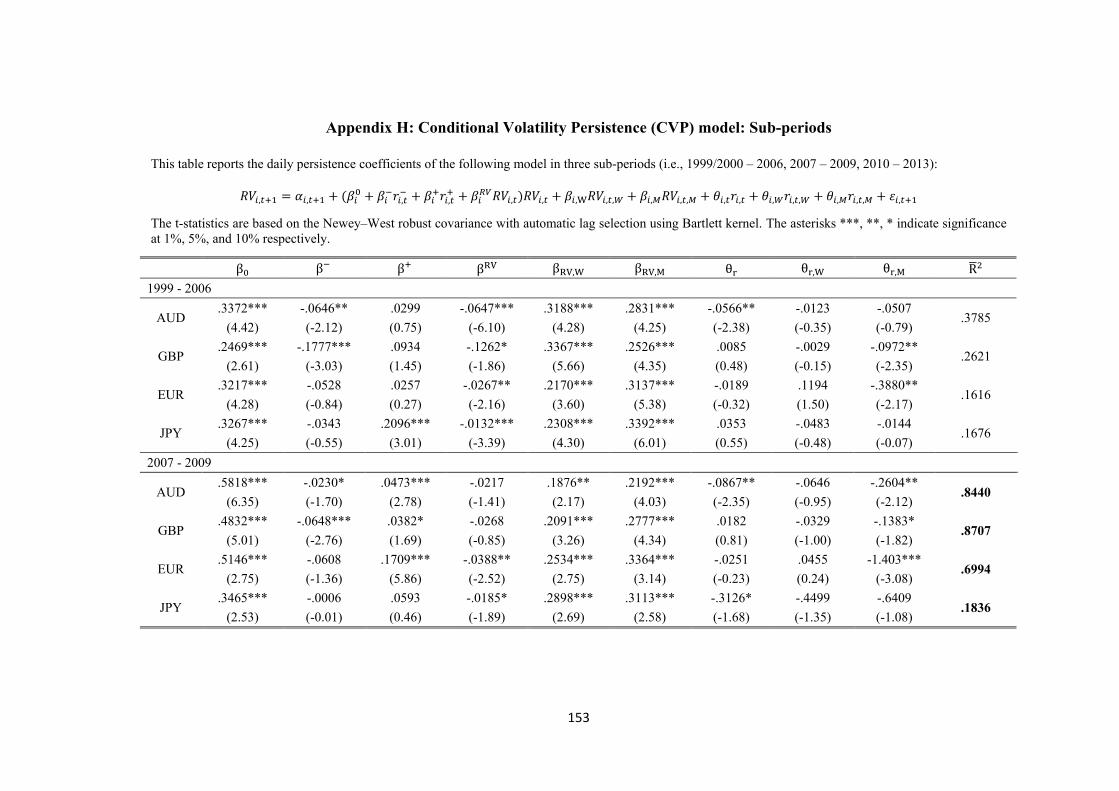
153

Appendix H: Conditional Volatility Persistence (CVP) model: Sub-periods

This table reports the daily persistence coefficients of the following model in three sub-periods (i.e., 1999/2000 – 2006, 2007 – 2009, 2010 – 2013):

𝑅𝑉𝑖,𝑡+1 = 𝛼𝑖,𝑡+1 + (𝛽𝑖0 + 𝛽𝑖



𝑅𝑉𝑅𝑉𝑖,𝑡)𝑅𝑉𝑖,𝑡 + 𝛽𝑖,W𝑅𝑉𝑖,𝑡,𝑊 + 𝛽𝑖,𝑀𝑅𝑉𝑖,𝑡,𝑀 + 𝜃𝑖,𝑡𝑟𝑖,𝑡 + 𝜃𝑖,𝑊𝑟𝑖,𝑡,𝑊 + 𝜃𝑖,𝑀𝑟𝑖,𝑡,𝑀 + 𝜀𝑖,𝑡+1

The t-statistics are based on the Newey–West robust covariance with automatic lag selection using Bartlett kernel. The asterisks ***, **, * indicate significance

at 1%, 5%, and 10% respectively.


1999 - 2006

AUD .3372*** -.0646** .0299 -.0647*** .3188*** .2831*** -.0566** -.0123 -.0507

.3785 (4.42) (-2.12) (0.75) (-6.10) (4.28) (4.25) (-2.38) (-0.35) (-0.79)

GBP .2469*** -.1777*** .0934 -.1262* .3367*** .2526*** .0085 -.0029 -.0972**

.2621 (2.61) (-3.03) (1.45) (-1.86) (5.66) (4.35) (0.48) (-0.15) (-2.35)

EUR .3217*** -.0528 .0257 -.0267** .2170*** .3137*** -.0189 .1194 -.3880**

.1616 (4.28) (-0.84) (0.27) (-2.16) (3.60) (5.38) (-0.32) (1.50) (-2.17)

JPY .3267*** -.0343 .2096*** -.0132*** .2308*** .3392*** .0353 -.0483 -.0144

.1676 (4.25) (-0.55) (3.01) (-3.39) (4.30) (6.01) (0.55) (-0.48) (-0.07)

2007 - 2009

AUD .5818*** -.0230* .0473*** -.0217 .1876** .2192*** -.0867** -.0646 -.2604**

.8440 (6.35) (-1.70) (2.78) (-1.41) (2.17) (4.03) (-2.35) (-0.95) (-2.12)

GBP .4832*** -.0648*** .0382* -.0268 .2091*** .2777*** .0182 -.0329 -.1383*

.8707 (5.01) (-2.76) (1.69) (-0.85) (3.26) (4.34) (0.81) (-1.00) (-1.82)

EUR .5146*** -.0608 .1709*** -.0388** .2534*** .3364*** -.0251 .0455 -1.403***

.6994 (2.75) (-1.36) (5.86) (-2.52) (2.75) (3.14) (-0.23) (0.24) (-3.08)

JPY .3465*** -.0006 .0593 -.0185* .2898*** .3113*** -.3126* -.4499 -.6409

.1836 (2.53) (-0.01) (0.46) (-1.89) (2.69) (2.58) (-1.68) (-1.35) (-1.08)

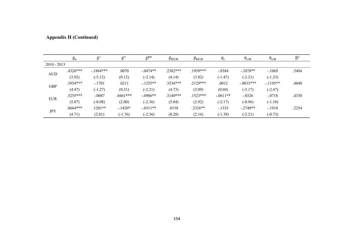
154

Appendix H (Continued)


2010 - 2013

AUD .4326*** -.1884*** .0070 -.0474** .2382*** .1959*** -.0384 -.1078** -.1069 .5404

(3.92) (-5.12) (0.12) (-2.14) (4.14) (3.82) (-1.47) (-2.21) (-1.23)

GBP .3954*** -.1701 .0211 -.1255** .3536*** .2129*** .0012 -.0833*** -.1195** .4840

(4.47) (-1.27) (0.31) (-2.21) (4.73) (3.09) (0.04) (-3.17) (-2.47)

EUR .5255*** -.0087 .0461*** -.0906** .3140*** .1523*** -.0611** -.0326 -.0718 .4330

(5.07) (-0.08) (2.00) (-2.36) (5.84) (2.92) (-2.17) (-0.96) (-1.10)

JPY .8664*** .1201** -.1420* -.0311** .0158 .2326** -.1335 -.2740** -.1910 .2254

(4.71) (2.01) (-1.76) (-2.36) (0.28) (2.16) (-1.38) (-2.21) (-0.73)

155

Bibliography

Admati, A. R., & Pfleiderer, P. (1988). A theory of intraday patterns: Volume and

price variability. Review of Financial Studies, 1(1), 3-40.

Adrian, T., & Rosenberg, J. (2008). Stock Returns and Volatility: Pricing the

Short‐Run and Long‐Run Components of Market Risk. The Journal of

Finance, 63(6), 2997-3030.

Ait-Sahalia, Y., & Brandt, M.W. (2001). Variable selection for portfolio choice.

The Journal of Finance, 56(4), 1297-1351.

Ait-Sahalia, Y., Mykland, P. A., & Zhang, L. (2005). How often to sample a

continuous-time process in the presence of market microstructure noise.

Review of Financial Studies, 18(2), 351-416.

Amihud, Y. (2002). Illiquidity and stock returns: cross-section and time series

effects. Journal of Financial Markets, 5, 31-56.

Andersen, T. G. (1996). Return volatility and trading volume: An information flow

interpretation of stochastic volatility. The Journal of Finance, 51(1), 169-204.

Andersen, T. G., & Bollerslev, T. (1997). Intraday periodicity and volatility

persistence in financial markets. Journal of Empirical Finance, 4(2), 115-158.

Andersen, T. G., & Bollerslev, T. (1998). Answering the skeptics: yes, standard

volatility models do provide accurate forecasts. International Economic

Review, 39, 885-905.

Andersen, T. G., & Bollerslev, T. (1998). Deutsche mark–dollar volatility: intraday

activity patterns, macroeconomic announcements, and longer run

dependencies. The Journal of Finance, 53(1), 219-265.

Andersen, T. G., Bollerslev, T., & Diebold, F. X. (2007). Roughing it up: Including

jump components in the measurement, modeling, and forecasting of return

volatility. The Review of Economics and Statistics, 89(4), 701-720.

156

Andersen, T. G., Bollerslev, T., Diebold, F. X., & Labys, P. (1999). Understanding,

optimizing, using and forecasting realized volatility and correlation. Working

Paper.

Andersen, T. G., Bollerslev, T., Diebold, F. X., & Labys, P. (2003). Modeling and

forecasting realized volatility. Econometrica, 71(2), 579-625.

Andersen, T. G., Bollerslev, T., Diebold, F. X., & Labys, P. (2011). The distribution

of realized exchange rate volatility. Journal of the American Statistical

Association, 96(453), 42-55.

Andersen, T. G., Bollerslev, T., Diebold, F. X., & Vega, C. (2007). Real-time price

discovery in global stock, bond and foreign exchange markets. Journal of

International Economics, 73(2), 251-277.

Andersen, T. G., Bollerslev, T., & Meddahi, N. (2005). Correcting the errors:

Volatility forecast evaluation using high‐frequency data and realized

volatilities. Econometrica, 73(1), 279-296.

Baillie, R. T., & Bollerslev, T. (1991). Intra-day and inter-market volatility in

foreign exchange rates. The Review of Economic Studies, 58(3), 565-585.

Balduzzi, P., & Lynch, A.W. (1999). Transaction costs and predictability: some

utility cost calculations. Journal of Financial Economics, 52, 47-78.

Bandi, F. M., & Russell, J. R. (2006). Separating market microstructure noise from

volatility. Journal of Financial Economics, 79, 655-692.

Bandi, F. M., & Russell, J. R. (2008). Microstructure noise, realized variance, and

optimal sampling. The Review of Economic Studies, 75(2), 339-369.

Bandi, F. M., Russell, J. R., & Zhu, Y. (2008). Using high-frequency data in

dynamic portfolio choice. Econometric Reviews, 27. 163-198.

Barberis, N. (2000). Investing for the long run when returns are predictable. The

Journal of Finance, 55, 225-264.

Barndorff-Nielsen, O. E., Hansen, P. R., Lunde, A., & Shephard, N. (2008).

Designing realized kernels to measure the ex post variation of equity prices in

the presence of noise. Econometrica, 76, 1481-1536.

157

Barndorff‐Nielsen, O. E., Hansen, P. R., Lunde, A., & Shephard, N. (2009).

Realized kernels in practice: Trades and quotes. The Econometrics Journal,

12(3), 1-32.

Barndorff-Nielsen, O. E., Kinnebrock, S., & Shephard, N. (2010). Measuring

downside risk –realised semivariance, in Bollerslev, T., Russell, J., & Watson,

M., eds., Volatility and Time Series Econometrics: Essays in Honor of Robert

F. Engle. New York: Oxford University Press.

Barndorff-Nielsen, O. E., & Shephard, N. (2002). Estimating quadratic variation

using realized variance. Journal of Applied Econometrics, 17(5), 457-477.

Battellino, R., & Plumb, M. (2011). A generation of an internationalised Australian

dollar. BIS Papers, 61, 202-217.

Berger, D., Chaboud, A., & Hjalmarsson, E. (2009). What drives volatility

persistence in the foreign exchange market? Journal of Financial Economics,

94(2), 192-213.

BIS. (2013). Triennial central bank survey of foreign exchange and derivatives

market activity in April 2013. Bank for International Settlements.

Bollerslev, T. (1986). Generalized autoregressive conditional heteroskedasticity.

Journal of Econometrics, 31(3), 307-327.

Bollerslev, T., Chou, R.Y., & Kroner, K. (1992). ARCH modeling in finance: A

review of the theory and empirical evidence. Journal of Econometrics, 52, 5-

59.

Bollerslev, T., & Domowitz, I. (1993). Trading patterns and prices in the interbank

foreign exchange market. The Journal of Finance, 48(4), 1421-1443.

Bollerslev, T., Engle, R. F., & Nelson, D. B. (1994). ARCH models. In Engle, R.F.

and McFadden, D., Eds., Handbook of Econometrics, Vol. IV, North-Holland,

Amsterdam.

Bollerslev, T., Hood, B., Huss J., & Pedersen, L. H. (2017). Risk everywhere:

Modeling and managing Volatility (March 21, 2017). SSRN Working Paper.

158

Booth, G. G., Lin, J. C., Martikainen, T., & Tse, Y. (2002). Trading and pricing in

upstairs and downstairs stock markets. Review of Financial Studies, 15(4),

1111-1135.

Bossaerts, P., & Hillion, P. (1999). Implementing statistical criteria to select return

forecasting models: what do we learn?. Review of Financial Studies, 12(2),

405-428.

Boucher, C., De Truchis, G., Dumitrescu, E., & Tokpavi, S. (2017). Testing for

Extreme Volatility Transmission with Realized Volatility Measures.

EconomiX Working Papers 2017-20, University of Paris Nanterre.

Brandt, M. W. (1999). Estimating portfolio and consumption choice: A conditional

Euler equations approach. The Journal of Finance, 54(5), 1609-1645.

Brandt, M. W., Kavajecz, K. A., & Underwood, S. E. (2007). Price discovery in the

treasury futures market. Journal of Futures Markets, 27(11), 1021-1051

Brennan, M.J. (1998). The role of learning in dynamic portfolio decisions.

European Finance Review, 1, 295-306.

Cai, F., Howorka, E., & Wongswan, J. (2008). Information linkages across trading

regions: Evidence from foreign exchange markets. Journal of International

Money and Finance, 27(8), 1215-1243.

Campbell, J. Y., Chan, Y. L., & Viceira, L. M. (2003). A multivariate model of

strategic asset allocation. Journal of Financial Economics, 67, 41-80.

Campbell, J. Y., & Viceria, L. M. (1999). Consumption and portfolio decisions

when expected returns are time varying. The Quarterly Journal of Economics,

114(2), 433-495.

Campbell, J. Y., & Viceria, L. M. (2002). Strategic asset allocation: portfolio

choice for long-term investors. Oxford University Press, Oxford, U.K.

Chai, E. F., Lee, A. D., & Wang, J. (2015). Global information distribution in the

gold OTC markets. International Review of Financial Analysis, 41, 206-217.

159

Chakrabarty, B., Pascual, R., & Shkilko, A. (2015). Evaluating trade classification

algorithms: bulk volume classification versus the tick rule and the Lee-Ready

algorithm. Journal of Financial Markets, 25, 52-79.

Chinn, M. D., & Ito, H. (2006). What matters for financial development? Capital

controls, institutions, and interactions. Journal of Development

Economics, 81(1), 163-192.

Clark, P. (1973). A subordinated stochastic process model with finite variance for

speculative prices. Econometrica, 41,135-155.

Corsi, F. (2009). A simple approximate long-memory model of realized

volatility. Journal of Financial Econometrics, 7(2), 174-196.

Corsi, F., & Reno, R. (2012). Discrete-time volatility forecasting with persistent

leverage effect and the link with continuous-time volatility modelling. Journal

of Business and Economic Statistics, 30(3), 368-380

Dacorogna, M. M., Müller, U. A., Nagler, R. J., Olsen, R. B., & Pictet, O. V. (1993).

A geographical model for the daily and weekly seasonal volatility in the foreign

exchange market. Journal of International Money and Finance, 12(4), 413-438.

Daniel, L., Kim, S. J., & McKenzie, M. D. (2014). The efficiency of the information

processing in the Australian Dollar market: Price discovery following

scheduled and unscheduled news. International Review of Financial

Analysis, 32, 159-178.

Das, S. R. (2002). The surprise element: jumps in interest rates. Journal of

Econometrics, 106(1), 27-65.

Debelle, G., Gyntelberg, J., & Plumb, M. (2006). Forward currency markets in Asia:

lessons from the Australian experience. BIS Quarterly Review, 53.

Diebold, F. X., & Lopez, J. A. (1995). Modeling volatility dynamics. In: Hoover,

K., Ed., Macroeconometrics: Developments, Tensions and Prospects, Kluwer

Academic Press, Boston, 427-466.

160

Diebold, F. X., & Nerlove, M. (1989). The dynamics of exchange rate volatility: a

multivariate latent factor ARCH model. Journal of Applied Econometrics, 4(1),

1-21.

Dominguez, K. M., & Panthaki, F. (2006). What defines ‘news’ in foreign exchange

markets? Journal of International Money and Finance, 25(1), 168-198.

Easley, D., De Prado, M. L., & O’Hara, M. (2016). Discerning information from

trade data. Journal of Financial Economics, 120(2), 269-286.

Easley, D., & O’Hara, M. (2005). Regulation and return: The role of ambiguity.

Working paper, Johnson GSM, Cornell University.

Edison, H. J., Cashin, P., & Liang, H. (2003). Foreign Exchange Intervention and

the Australian Dollar: Has it Mattered?. IMF Working Papers, 2003(99).

Ehlers, T., & Packer, F. (2013). FX and derivatives markets in emerging economies

and the internationalisation of their currencies. BIS Quarterly Review,

December.

Ehrmann , M., & Fratzscher, M. (2005). Exchange rates and fundamentals: new

evidence from real-time data. Journal of International Money and Finance,

24(2), 317-341.

Engle, R. F., Ito, T., & Lin, W. L. (1990). Meteor showers or heat waves?

heteroskedastic intra-daily volatility in the foreign exchange

market. Econometrica, 58, 525-542.

Engle, R. F. (1982). Autoregressive conditional heteroscedasticity with estimates

of the variance of United Kingdom inflation. Econometrica, 50, 987-1007.

Eraker, B., Johannes, M., & Polson, N. (2003). The impact of jumps in volatility

and returns. The Journal of Finance, 58(3), 1269-1300.

Erdemlioglu, D., Laurent, S., & Neely, C. J. (2012). Econometric modeling of

exchange rate volatility and jumps. Federal Reserve Bank of St. Louis.

Working Paper 2012-008A.

Evans, M. D., (2002), FX trading and exchange rate dynamics. Journal of Finance,

57(6), 2405–2447.

161

Evans, M. D., & Lyons, R. K. (1999). Microstructure meets asset pricing: Order

flow effects in the FX market. MIMEO.

Evans, M. D., & Lyons, R. K. (2001). Portfolio balance, price impact, and secret

intervention (July 2001). NBER Working Paper No. 8356.

Evans, M. D., & Lyons, R. K. (2002a). Informational integration and FX trading.

Journal of International Money and Finance, 21(6), 807-831.

Evans, M. D., & Lyons, R. K. (2002b). Time-varying liquidity in foreign exchange.

Journal of Monetary Economics, 49(5), 1025-1051.

Evans, M. D., & Lyons, R. K. (2005). Do currency markets absorb news quickly?

Journal of International Money and Finance, 24(2), 197-217.

Evans, M. D., & Lyons, R. K. (2008). How is macro news transmitted to exchange

rates? Journal of Financial Economics, 88(1), 26-50.

Fleming, J., & Kirby, C. (2011). Long memory in volatility and trading volume.

Journal of Banking & Finance, 35(7), 1714-1726.

Fleming, J., Kirby, C., & Ostdiek, B. (2001). The economic value of volatility

timing. Journal of Finance, 56(1), 329-352.

Fleming, J., Kirby, C., & Ostdiek, B. (2003). The economic value of volatility

timing using ‘realized’ volatility. Journal of Financial Economics, 67(3), 473-

509.

Fleming, M. J., & Piazzesi, M. (2005). Monetary policy tick-by-tick. Unpublished

paper, August 2005.

Forsberg, L., & Ghysels, E. (2007). Why do absolute returns predict volatility so

well? Journal of Financial Econometrics, 5(1), 31-67.

Fricke, C., & Menkhoff, L. (2011). Does the “Bund” dominate price discovery in

Euro bond futures? Examining information shares. Journal of Banking &

Finance, 35(5), 1057-1072.

Frijns, B., Gilbert, A., & Tourani-Rad, A. (2010). The dynamics of price discovery

for cross-listed shares: evidence from Australia and New Zealand. Journal of

Banking & Finance, 34(3), 498-508.

162

Frijns, B., Indriawan, I., & Tourani-Rad, A. (2015). Macroeconomic news

announcements and price discovery: Evidence from Canadian–US cross-listed

firms. Journal of Empirical Finance, 32, 35-48.

Frijns, B., Lehnert, T., & Zwinkels, R. (2010). Behavioral heterogeneity in the

option market. Journal of Economic Dynamics and Control,34(11), 2273-2287.

Gau, Y. & Wu, Z. (2017). Macroeconomic announcements and price discovery in

the foreign exchange market. Journal of International Money and Finance,

79(C), 232-254.

Giacomini, R., & White, H. (2006). Tests of conditional predictive ability.

Econometrica, 74(6), 1545-1578.

Gillemot, L., Farmer, J. D., & Lillo, F. (2006). There is more volatility than volume.

Quantitative Finance, 6(5), 371-384.

Glick, R., & Rose, A. K. (1999). Contagion and trade: Why are currency crises

regional? Journal of International Money and Finance, 18(4), 603-617.

Glosten, L. R., Jagannathan, R., & Runkle, D. E. (1993). On the relation between

the expected value and the volatility of the nominal excess return on stocks.

The Journal of Finance, 48(5), 1779-1801.

Glosten, L. R., & Milgrom, P. R. (1985). Bid, ask and transaction prices in a

specialist market with heterogeneously informed traders. Journal of Financial

Economics, 14(1), 71-100.

Goodhart, C. A., & O'Hara, M. (1997). High frequency data in financial markets:

Issues and applications. Journal of Empirical Finance, 4(2), 73-114.

Grammig, J., Melvin, M., & Schlag, C. (2005). Internationally cross-listed stock

prices during overlapping trading hours: Price discovery and exchange rate

effects. Journal of Empirical Finance, 12(1), 139-164.

Green, T. C. (2004). Economic news and the impact of trading on bond prices. The

Journal of Finance, 59(3), 1201-1234.

Hansen, P. R., & Lunde, A. (2003). An unbiased measure of realized variance

(March 31, 2004). SSRN Working Paper.

163

Hansen, P. R., & Lunde, A. (2005). A forecast comparison of volatility models:

Does anything beat a GARCH (1, 1)? Journal of Applied Econometrics, 20(7),

873-889.

Hansen, P. R., & Lunde, A. (2006). Realized variance and market microstructure

noise. Journal of Business & Economic Statistics, 24(2), 127-161.

Harvey, C. R., & Huang, R. D. (1991). Volatility in the foreign currency futures

market. The Review of Financial Studies, 4(3), 543-569.

Hasbrouck, J. (1995). One security, many markets: Determining the contributions

to price discovery. The Journal of Finance, 50, 1175-1199.

Hasbrouck, J. (2003). Intraday price formation in US equity index markets. The


He, X., & Velu, R. (2014). Volume and volatility in a common-factor mixture of

distributions model. Journal of Financial and Quantitative Analysis, 49, 33–

49

Hendershott, T., & Jones, C. M. (2005). Trade-through prohibitions and market

quality. Journal of Financial Markets, 8(1), 1-23.

Hogan, K. C., & Melvin, M. T. (1994). Sources of meteor showers and heat waves

in the foreign exchange market. Journal of International Economics, 37(3-4):

239-247.

Huang, R. D. (2002). The quality of ECN and Nasdaq market maker quotes. The


Ito, T., Engle, R. F., & Lin, W. L. (1992). Where does the meteor shower come

from? The role of stochastic policy coordination. Journal of International

Economics, 32(3-4), 221-240.

Ito, T., Lyons, R. K., & Melvin, M. T. (1998). Is there private information in the

FX market? The Tokyo experiment. The Journal of Finance, 53(3), 1111-1130.

Jiang, G., Lo, I., & Valente, G. (2014). High-frequency trading around

macroeconomic news announcements: Evidence from the US treasury market.

Bank of Canada Working Paper.

164

Johannes, M. S., Polson, N., & Stroud, J. R. (2002). Sequential Optimal Portfolio

Performance: Market and Volatility Timing (February 2002). SSRN Working

Paper.

Kaminsky, G. L., & Reinhart, C. M. (2002). Financial markets in times of stress.

Journal of Development Economics, 69(2), 451-470.

Killeen, W. P., Lyons, R. K., & Moore, M. J. (2006). Fixed versus flexible: Lessons

from EMS order flow. Journal of International Money and Finance, 25(4),

551-579.

King, M. R., Osler, C., & Rime, D. (2011). Foreign Exchange Market Structure,

Players, and Evolution. Handbook of Exchange Rates, John Wiley & Sons, Inc:

1-44.

King, Sarno, & Sojli (2010). Timing exchange rates using order flow: The case of

the Loonie. Journal of Banking & Finance, 34(12), 2917-2928.

Kyle, A. S. (1985). Continuous auctions and insider trading. Econometrica, 53(6),

1315-1335.

Lahaye, J., & Neely, C. J. (2016). The role of jumps in volatility spillovers in

foreign exchange markets: Meteor shower and heat waves revisited. Federal

Reserve Bank of St. Louis Working Paper Series (2014-034B).

Laurent, S., Rombouts, J. V. K., & Violante, F. (2012). On the forecasting accuracy

of multivariate GARCH models. Journal of Applied Econometrics, 27(6), 934-

955.

Lee, C., & Ready, M. J. (1991). Inferring trade direction from intraday data. The


Liesenfeld, R. (2001). A generalized bivariate mixture model for stock price

volatility and trading volume. Journal of Econometrics, 104(1), 141-178.

Lin, J. C., Sanger, G. C., & Booth, G. G. (1995). Trade size and components of the

bid-ask spread. The Review of Financial Studies, 8(4), 1153-1183.

Lindeman, R. H., Merenda, P. F., & Gold, R. Z. (1980). Introduction to bivariate

and multivariate analysis. Scott Foresman Glenview, IL.

165

Liu, L. Y., Patton, A. J., & Sheppard, K. (2015). Does anything beat 5-minute RV?

A comparison of realized measures across multiple asset classes. Journal of

Econometrics, 187(1), 293-311.

Love, R., & Payne, R. (2008). Macroeconomic news, order flows, and exchange

rates. Journal of Financial and Quantitative Analysis, 43(02), 467-488.

Marquering, W., & Verbeek, M. (2004). The economic value of predicting stock

index returns and volatility. Journal of Financial and Quantitative Analysis,

39, 2407-2429.

McAleer, M., & Medeiros, M. C. (2008). Realized volatility: A review.

Econometric Reviews, 27(1-3), 10-45.

McCauley, R. (2006). Internationalising a currency: The case of the Australian

dollar. BIS Quarterly Review, December 2006, 41-54.

Meese, R. A., & Rogoff, K. S. (1983). Empirical exchange rate models of the

seventies: Are any fit to survive? Journal of International Economics, (14), 3-

24.

Melvin, M., & Yin, X. (2000). Public information arrival, exchange rate volatility,

and quote frequency. The Economic Journal, 110(465), 644-661.

Melvin, M., & Melvin, B. P. (2003). The global transmission of volatility in the

foreign exchange market. The Review of Economics and Statistics, 85(3), 670-

679.

Menkveld, A. J., Sarkar, A., & Wel, M. V. D. (2012). Customer order flow,

intermediaries, and discovery of the equilibrium risk-free rate. Journal of

Financial and Quantitative Analysis, 47(04), 821-849.

Merton, R. C. (1980). On estimating the expected return on the market: An

exploratory investigation. Journal of Financial Economics, 8(4), 323-361.

Mizrach, B., & Neely, C. J. (2008). Information shares in the US Treasury market.

Journal of Banking & Finance, 32(7), 1221-1233.

166

Moshirian, F., Nguyen, H.G., & Pham, P.K. (2012). Overnight public information,

order placement, and price discovery during pre-opening period. Journal of

Banking & Finance, 36(10), 2837-2851.

Müller, U. A., Dacorogna, M. M., Davé, R. D., Olsen, R. B., Pictet, O. V., & von

Weizsäcker, J. E. (1997). Volatilities of different time resolutions — Analyzing

the dynamics of market components. Journal of Empirical Finance, 4(2), 213-

239.

Ning, C., Xu, D., & Wirjanto, T. S. (2015). Is volatility clustering of asset returns

asymmetric?. Journal of Banking & Finance, 52, 62-76.

Nolte, I., & Xu, Q. (2015). The economic value of volatility timing with realized

jumps. Journal of Empirical Finance, 34, 45–59

Pascual, R., Pascual-Fuster, B., & Climent, F. (2006). Cross-listing, price discovery

and the informativeness of the trading process. Journal of Financial Markets,

9(2), 144-161.

Pasquariello, P., & Vega, C. (2007). Informed and strategic order flow in the bond

markets. The Review of Financial Studies, 20(6), 1975-2019.

Patel, V., Putniņš, T. J., & Michayluk, D. (2014). Price discovery in stock and

options markets (February 2, 2018). SSRN Working Paper.

Patton, A.J., & Sheppard, K. (2009). Optimal combinations of realised volatility

estimators. International Journal of Forecasting, 25, 218-238.

Patton, A.J., & Sheppard, K. (2015). Good volatility, bad volatility: Signed jumps

and the persistence of volatility. The Review of Economics and Statistics, 97(3),

683–697.

Peng, L., & Xiong, W. (2006). Investor attention, overconfidence and category

learning. Journal of Financial Economics, 80(3), 563-602.

Rime, D., & Schrimpf, A. (2013). The anatomy of the global FX market through

the lens of the 2013 Triennial Survey. BIS Quarterly Review, December 2013,

27-43.

Sassen, S. (1999). Global financial centers. Foreign Affairs, 75-87.

167

Sharpe, W. F. (1966). Mutual Fund Performance. Journal of Business, 119-138.

Stambaugh, R. F. (1999). Predictive regressions. Journal of Financial Economics,

54(3), 375-421.

Su, F. (2017). Conditional volatility persistence and volatility timing in the foreign

exchange market. Unpublished paper.

Su, F., & Wang, J. (2017). Conditional volatility persistence in the foreign

exchange market: Meteor shower and heat wave revisited (December 7, 2017).

SSRN Working Paper.

Su, F., & Zhang, J. (2018). Global price discovery in the Australian dollar market

and its determinants. Pacific-Basin Finance Journal, 48, 35-55.

Tauchen, G. E. and M. Pitts (1983). The price variability-volume relationship on

speculative markets. Econometrica, 51(2), 485-505.

Thomakos, D.D., & Wang, T. (2010). Volatility Timing and Portfolio Construction

Using Realized Volatility for the S&P500 Futures Index. In: Guerard J.B. (eds)

Handbook of Portfolio Construction. Springer, Boston, MA.

Upper, C., & Werner, T. (2002). Tail wags dog? Time-varying information shares

in the Bund market. Economic Research Centre Working Paper (24/02),

Deutsche Bundesbank.

Wang, J. (2014). Overnight price discovery and the internationalization of a

currency: The case of the Korean Won. Pacific-Basin Finance Journal, 29(1),

86-95.

Wang, J., & Yang, M. (2009). Asymmetric volatility in the foreign exchange

markets. Journal of International Financial Markets, Institutions & Money,

19(4), 597-615.

Wang, J., & Yang, M. (2011). Housewives of Tokyo versus the gnomes of Zurich:

Measuring price discovery in sequential markets. Journal of Financial Markets,

14(1), 82-108.

Wang, J., & Yang, M. (2013). On the risk return relationship. Journal of Empirical

Finance, 21, 132-141.

168

Wang, J., & Yang, M. (2017). Conditional Volatility Persistence. Unpublished

paper.

Wintoki, M., Linck, J., & Netter, J. (2012). Endogeneity and the dynamics of

internal corporate governance. Journal of Financial Economics, 105, 581-606.

Yin, X. (2005). A comparison of centralized and fragmented markets with costly

search. The Journal of Finance, 60(3), 1567-1590.

Zhang, L., Mykland P. A., & Aït-Sahalia Y. (2005). A tale of two time scales:

Determining integrated volatility with noisy high-frequency data. Journal of

the American Statistical Association, 100(472), 1394-1411.

essays on price discovery and volatility dynamics in the

Documents