four essays on the econometric analysis of high-frequency ... · four essays on the econometric...
TRANSCRIPT

Four Essays on the EconometricAnalysis of High-Frequency Order Data
DISSERTATION
zur Erlangung des akademischen Gradesdoctor rerum politicarum
(Doktor der Wirtschaftswissenschaft)
eingereicht an derWirtschaftswissenschaftlichen Fakultatder Humboldt-Universitat zu Berlin
vonM. Sc Ruihong Huang
geboren am 27.08.1976 in Fujian, China
Prasident der Humboldt-Universitat zu Berlin:Prof. Dr. Jan-Hendrik Olbertz
Dekan der Wirtschaftswissenschaftlichen Fakultat:Prof. Oliver Gunther, Ph.D.
Gutachter:
1. Prof. Dr. Nikolaus Hautsch
2. Prof. Dr. Christian T. Brownlees
Tag des Kolloquiums: 14 Februar, 2012


Abstract
Electronic limit order markets account for a large and increasing percentage ofglobal financial trading. Understanding the complex interaction between traders’limit order submission strategies and the state of the market, and their consequenteffects on market quality becomes increasingly important for investors, as well asto those who regulate and design automated markets.
In four essays, this thesis examines the aforementioned interaction by econo-metric analysis of the market impact of limit order, the properties of order flowand traders’ (hidden) order submission decisions.
Chapter 1 looks at the market impact of limit orders. Quantifying short-term and long-term effects of limit order submissions on quotes in Euronext, weshow that limit orders have significant information content, and how strongly limitorders signal the market depends on both their characteritics (price and size) andthe state of limit order books (LOBs).
Chapter 2 provides new empirical evidence on order submission activities andmarket impacts of limit orders at NASDAQ. We find that traders dominantly sub-mit small size limit orders and cancell most of them immediately after submission.Based on the estimated market impact of orders, we propose a method to predictthe optimal size of a limit order conditional on its position in the LOB and a givenfixed level of expected impact.
Chapter 3 analyzes traders’ decisions on using undisclosed orders in opaquemarkets. Employing Totalview message data at NASDAQ, we show that marketconditions affect traders’ order submission strategies and thus the location of hid-den liqudity is predictable given observable market characteristics. Out evidencealso suggests that traders balance their hidden order placements to compete forthe provision of liquidity and protect themselves against picking-off risk.
Chapter 4 presents a program framework for reconstructing LOBs as well asextracting order flow information from message stream data. We design the basicmodules of the system in an abstract layer based on common order events inlimit order markets, so that it can be easily adapted to data at any limit ordermarkets. The underlying data structure is highly optimized and the programs inthese modules are exhaustively tested to guarantee the high reliablity and efficiencyof the system.
I

II

Zusammenfassung
Transaktionen auf vollstandig elektronischen, Limit-Order -getriebenen Marktenmachen einen großen und wachsenden Teil aller weltweiten Finanzmarkttransak-tionen aus. Es ist deshalb von herausragender Bedeutung fur Investoren undRegulatoren dieser Markte, die komplexen Interaktionen zwischen dem Zustanddes Marktes und den Limit-Ordern der Marktteilnehmer zu verstehen.
Das Kapitel 1 befasst sich mit den Auswirkungen von Limit-Ordern der Mark-tteilnehmer auf den Zustand des Marktes und die Marktqualitat. In der Analysequantifizieren wir die kurz- und langfristigen Effekte der Limit-Order Platzierungauf Preisquotierungen. Am Beispiel des Borsenplatzes Euronext zeigen wir, dasseine Limit-Order signifikante Informationen fur Preisquotierungen enthalt und il-lustrieren inwieweit der Markt von den Charakteristika der Limit-Order (Preis undVolumen) und dem Zustand des Orderbuchs abhangt.
Das Kapitel 2 enthalt neue empirische Resultate uber die Limit-Order Ak-tivitat und den Markteinfluss von Limit-Ordern an der New Yorker NASDAQBorse. Wir dokumentieren, dass Marktteilnehmer hauptsachlich die Platzierungvon Limit-Ordern mit kleinen Volumina praferieren, diese aber haufig sofort nachihrem Einsatz wieder loschen. Basierend auf der geschatzten Marktauswirkungeiner individuellen Limit-Order schlagen wir eine Methode zur Prognose des opti-malen Volumens einer Limit-Order vor. Die optimalen Eigenschaften der Limit-Order hangen dabei von der Position im Orderbuch sowie der vorab spezifiziertenerwarteten bzw. praferierten Marktauswirkung ab.
Im Kapitel 3 werden die Limit-Order-Strategien von Marktteilnehmern inintransparenten Markten untersucht. Unter Benutzung des Totalview messageDatensatzes des NASDAQ Borsenplatzes zeigen wir, dass die Position der soge-nannten versteckten Liquiditat im Orderbuch von diversen Variablen abhangt, dieden Zustand des Marktes beschreiben. Insbesondere zeigen wir, dass die Posi-tion der versteckten Liquiditat prognostizierbar ist. Die Daten suggerieren zudem,dass Handler die Platzierung sogenannter Hidden-Orders im Hinblick auf gunstigeLiquiditat am Markt und dem ”‘Picking-Off”’-Risiko ausbalancieren.
Im letzten Kapitel 4 prasentieren wir ein Softwaresystem zur Rekonstruktionvon Orderbuchern und zur Extrahierung von Orderflussinformationen aus messagestream Daten fur Limit-Orders. Die Basismodule des Systems beruhen auf allge-meinen Orderbuch-Ereignissen. Sie sind abstrakt gehalten und konnen so einfachauf beliebige Markte mit elektronischen Orderbuchern angewendet werden. Diegrundlegende Struktur ist im Hinblick auf Anwendbarkeit optimiert und grundlichgetestet worden um eine hohe Verlasslichkeit und Effizienz zu gewahrleisten.
III

IV

AcknowledgmentI owe a measure of gratitude to several people, without whom this thesis would
not have been completed.First of all, I am very grateful to my supervisor, Nikolaus Hautsch, for his
inspiring and encouraging advice. I very much benefited from numerous insightfuldiscussions with him. He offered an excellent and exciting research environmentat his Chair.
I am greatly indebted to my second advisor, Christian Brownlees for his valu-able input. The discussion with him was not only academically fruitful but alsopersonally enjoyable.
This thesis would not have been possible without the many insights that Ilearned from my colleagues and friends working in the financial industry. I es-pecially appreciate the enlightened talk, the strong expression of interest and thevaluable constructive criticism that they have given me. I wish to acknowledge thefollowing persons by name: Andrew Ferraris (UBS Investment Bank), Lada Kyj(Barclays Capital), Daniel Nehren (JP Morgan Chase), Artem Novikov (TradingPhysics), Roel Oomen (Deutsche Bank) and Dmitry Shakin (GSA Capital).
Many thanks are due to my colleagues at the “Lehrstuhl fur Okonometrie”who actively commented on my research: Bernd Droge, Axel Groß-Klußmann,Gustav Haitz, Franziska Lottmann, Peter Malec, Tomas Polak, Julia Schaumburgand Melanie Schienle. I also owe special debt to the entire LOBSTER develop-ment team including Gustav, Tomas and two student assistants, Jonas Haase andGagandeep Singh.
I heavily benefited from the financial support by Deutsche Bank and from thestimulating atmosphere within the Quantitative Products Laboratory (QPL). Iespecially appreciate the impressive scientific activities organized by two scientificdirectors, Ulrich Horst and Peter Bank, and the operation official, Almut Birsner.Besides, I owe debt to all colleagues in QPL for giving me the wonderful experienceboth in my academic career and in my social life. Among them, I would like toespecially thank Gokhan Cebiroglu, Mstislav Elagin, Antje Fruth, Peter Kratz,Felix Naujokat, Michael Paulsen and Nick Westray for all inspiring discussionsduring working time and lunchs.
Finally and most of all, I would like to thank my wife, Xi, who not only con-sistently supported and encouraged me during the last four years but also broughtme my sweet daughter, Sophie. They gave me the mental support, optimism, andretreat that enabled me to successfully finish my dissertation.
V

VI

Contents
Introduction 2
1 Market Impact of a Limit Order 51.1 Introduction . . . . . . . . . . . . . . . . . . . . . . . . . . . . . . . 51.2 Data and Market Environment . . . . . . . . . . . . . . . . . . . . 71.3 Econometric Modelling . . . . . . . . . . . . . . . . . . . . . . . . . 10
1.3.1 A Cointegrated VAR Model for Quotes and Depths . . . . . 101.3.2 Limit Orders as Shocks to the System . . . . . . . . . . . . . 121.3.3 Measuring the Market Impact . . . . . . . . . . . . . . . . . 15
1.4 Estimation Results . . . . . . . . . . . . . . . . . . . . . . . . . . . 181.4.1 Statistical Properties of Market Depth . . . . . . . . . . . . 191.4.2 Estimated Cointegration Relations . . . . . . . . . . . . . . 21
1.5 Estimated Market Impact . . . . . . . . . . . . . . . . . . . . . . . 231.5.1 Limit Orders Placed At or Behind the Market . . . . . . . . 231.5.2 Limit Orders Placed Inside Of the Spread . . . . . . . . . . 281.5.3 Market Impact of Trades . . . . . . . . . . . . . . . . . . . . 291.5.4 Robustness of Results . . . . . . . . . . . . . . . . . . . . . 331.5.5 Cross-Sectional Evidence . . . . . . . . . . . . . . . . . . . . 33
1.6 Conclusion . . . . . . . . . . . . . . . . . . . . . . . . . . . . . . . . 36
2 Limit Order Properties and Optimal Order Sizes 372.1 Introduction . . . . . . . . . . . . . . . . . . . . . . . . . . . . . . . 372.2 Market Environment and Data . . . . . . . . . . . . . . . . . . . . 392.3 Major Order Flow and Order Book Characteristics . . . . . . . . . 402.4 An Econometric Model for the Market Impact of Limit Orders . . . 44
2.4.1 A Cointegrated VAR Model for the Limit Order Book . . . . 442.4.2 Estimating Market Impact . . . . . . . . . . . . . . . . . . . 47
2.5 Market Impact at NASDAQ . . . . . . . . . . . . . . . . . . . . . . 512.6 Optimal Order Size . . . . . . . . . . . . . . . . . . . . . . . . . . . 552.7 Conclusion . . . . . . . . . . . . . . . . . . . . . . . . . . . . . . . . 58
VII

3 Identifying and Analyzing Hidden Order Placements 613.1 Introduction . . . . . . . . . . . . . . . . . . . . . . . . . . . . . . . 613.2 Economic Reasoning of Optimal Order Display . . . . . . . . . . . 64
3.2.1 Theories on Undisclosed Orders . . . . . . . . . . . . . . . . 643.2.2 Empirical Evidences on Undisclosed Orders . . . . . . . . . 653.2.3 Testable Hypotheses . . . . . . . . . . . . . . . . . . . . . . 66
3.3 Measuring Hidden Order Locations . . . . . . . . . . . . . . . . . . 693.3.1 Institutional Background . . . . . . . . . . . . . . . . . . . . 693.3.2 Data . . . . . . . . . . . . . . . . . . . . . . . . . . . . . . . 693.3.3 Identifying Undisclosed Orders . . . . . . . . . . . . . . . . . 723.3.4 Measuring the Aggressiveness of Undisclosed Orders . . . . . 753.3.5 Capturing Market Conditions . . . . . . . . . . . . . . . . . 80
3.4 Econometric Modelling . . . . . . . . . . . . . . . . . . . . . . . . . 813.4.1 An Ordered Probit Model with Censoring . . . . . . . . . . 813.4.2 Cross-Sectional Aggregation . . . . . . . . . . . . . . . . . . 83
3.5 Empirical Evidence . . . . . . . . . . . . . . . . . . . . . . . . . . . 833.5.1 Hidden Order Placements in Dependence of Spread Sizes . . 843.5.2 (How) Does Hidden Liquidity Compete with Visible Liquid-
ity Provision? . . . . . . . . . . . . . . . . . . . . . . . . . . 883.5.3 Hidden Order Placements After Price Movements and Trad-
ing Signals . . . . . . . . . . . . . . . . . . . . . . . . . . . . 903.5.4 Competition for Hidden Liquidity Provision . . . . . . . . . 913.5.5 Hidden Order Placements and HFT . . . . . . . . . . . . . . 913.5.6 Intraday Patterns . . . . . . . . . . . . . . . . . . . . . . . . 92
3.6 Conclusion . . . . . . . . . . . . . . . . . . . . . . . . . . . . . . . . 92
4 Extracting Information from the Message Stream 934.1 Introduction . . . . . . . . . . . . . . . . . . . . . . . . . . . . . . . 934.2 Message Stream Data . . . . . . . . . . . . . . . . . . . . . . . . . . 944.3 Overview of LOBSTER . . . . . . . . . . . . . . . . . . . . . . . . . 984.4 Limit Order Book Reconstruction . . . . . . . . . . . . . . . . . . . 101
4.4.1 Overview of the Reconstruction Procedure . . . . . . . . . . 1014.4.2 Implementation of LOB Constructor . . . . . . . . . . . . . 1014.4.3 Output of LOB Constructor . . . . . . . . . . . . . . . . . . 1034.4.4 Application: Visualization of LOB and Order Flow . . . . . 107
4.5 Order Tracer . . . . . . . . . . . . . . . . . . . . . . . . . . . . . . 1074.5.1 Implementation of Order Tracer . . . . . . . . . . . . . . . . 1074.5.2 Output of Order Tracer . . . . . . . . . . . . . . . . . . . . 1094.5.3 Application: Main Characteristics of Limit Orders . . . . . . 112
4.6 Conclusion . . . . . . . . . . . . . . . . . . . . . . . . . . . . . . . . 113
VIII

Bibliography 119
A 121A.1 Adaptive time window matching algorithm . . . . . . . . . . . . . . 121A.2 FIML estimator for cointegrating vectors . . . . . . . . . . . . . . . 122A.3 Transform estimates from VECM to VAR . . . . . . . . . . . . . . 123
B 125B.1 Asymptotic Distribution of Marginal Effects . . . . . . . . . . . . . 125B.2 Histogram of Significant Ordered Probit Estimates . . . . . . . . . 126
IX

X
List of Figures
1.1 Scenario 1a (normal limit order) . . . . . . . . . . . . . . . . . . . . 131.2 Scenario 2 (aggressive limit order) . . . . . . . . . . . . . . . . . . . 131.3 Scenario 3 (normal market order) . . . . . . . . . . . . . . . . . . . 141.4 Scenario 4 (aggressive market order) . . . . . . . . . . . . . . . . . 141.5 Time series plot of log market depths . . . . . . . . . . . . . . . . . 191.6 Density and autocorrelation of market depths . . . . . . . . . . . . 201.7 Time series of estimated cointegration relations . . . . . . . . . . . 241.8 Market impact of normal limit orders . . . . . . . . . . . . . . . . . 251.9 Market impact of limit orders posted behind the market . . . . . . 271.10 Market impact of aggressive limit orders . . . . . . . . . . . . . . . 281.11 Market impact of normal market orders . . . . . . . . . . . . . . . . 291.12 Market impact of aggressive market orders . . . . . . . . . . . . . . 311.13 Comparison of market impacts of market orders and limit orders . . 321.14 Robustness of results . . . . . . . . . . . . . . . . . . . . . . . . . . 33
2.1 Histogram of order sizes, execution sizes, cancellation times andexecution times of limit orders . . . . . . . . . . . . . . . . . . . . . 41
2.2 Scenario 1a (normal limit order) . . . . . . . . . . . . . . . . . . . . 482.3 Scenario 2 (aggressive limit order) . . . . . . . . . . . . . . . . . . . 492.4 Scenario 3 (normal market order) . . . . . . . . . . . . . . . . . . . 492.5 Market impact of normal limit orders (NASDAQ) . . . . . . . . . . 522.6 Market impact of limit orders posted behind the market (NASDAQ) 532.7 Market impact of aggressive limit orders (NASDAQ) . . . . . . . . 542.8 Comparison of market impacts of market orders and limit orders
(NASDAQ) . . . . . . . . . . . . . . . . . . . . . . . . . . . . . . . 552.9 Permanent impacts against order sizes . . . . . . . . . . . . . . . . 57
3.1 Percentage of trading volumes executed against hidden depth . . . . 633.2 Stylized trading scenario of executing hidden orders . . . . . . . . . 733.3 Stylized trading scenario of aggressive limit order submissions . . . 743.4 Stylized trading secnario of market order submissions . . . . . . . . 743.5 Illustration of the hidden order aggressiveness measure s . . . . . . 75
XI

3.6 Illustration of the hidden order aggressiveness measure d . . . . . . 773.7 Stylized illustration of the effect of a widening of bid-ask spreads on
hidden order placements for large-spread stocks . . . . . . . . . . . 883.8 Stylized illustration of the effect of an increase of visible ask depth
on undisclosed buy order placements for medium-spread stocks . . . 893.9 Stylized illustration of the effect of an increase of visible ask depth
on undisclosed buy order placements for large-spread stocks . . . . 89
4.1 A sequence of messages related to the same limit order . . . . . . . 964.2 Comparison of TAQ and one-level LOB generated by LOBSTER . . 974.3 The overview of LOBSTER system . . . . . . . . . . . . . . . . . . 984.4 LOB reconstruction procedure . . . . . . . . . . . . . . . . . . . . . 1004.5 Sequential diagram for messages of limit order executions . . . . . . 1024.6 Class diagram of LOB construction . . . . . . . . . . . . . . . . . . 1034.7 The visualization of LOB and order flow . . . . . . . . . . . . . . . 1084.8 Class diagram of trace construction . . . . . . . . . . . . . . . . . . 1094.9 Histogram of limit orders’ characteristics . . . . . . . . . . . . . . . 112
A.1 Histogram of the delay time between trades and corresponding LOBupdating . . . . . . . . . . . . . . . . . . . . . . . . . . . . . . . . . 122
B.1 The histogram of significant estimates (1) . . . . . . . . . . . . . . 127B.2 The histogram of significant estimates (2) . . . . . . . . . . . . . . 128B.3 The histogram of significant estimates (3) . . . . . . . . . . . . . . 129B.4 The histogram of significant estimates (4) . . . . . . . . . . . . . . 130
XII

List of Tables
1.1 Summary of synchronized trade and order book data . . . . . . . . 91.2 Variable definitions . . . . . . . . . . . . . . . . . . . . . . . . . . . 101.3 Shock vectors implied by the underlying five scenarios . . . . . . . . 161.4 Stationarity tests on quotes and market depths . . . . . . . . . . . 201.5 Representative estimates of cointegrating vectors . . . . . . . . . . . 211.6 Representative estimates of the loading matrix . . . . . . . . . . . . 221.7 Cross-sectional analysis of market impacts over the market . . . . . 35
2.1 Summary statistics of selected stocks . . . . . . . . . . . . . . . . . 402.2 Limit order activities at NASDAQ . . . . . . . . . . . . . . . . . . . 422.3 Market order activities . . . . . . . . . . . . . . . . . . . . . . . . . 442.4 Summary of order books (NASDAQ) . . . . . . . . . . . . . . . . . 452.5 Representative estimates of cointegrating vectors (NASDAQ) . . . . 472.6 Shock vectors implied by the underlying four scenarios . . . . . . . 50
3.1 Cross-sectional summary statistics on the characteristics of the se-lected stocks . . . . . . . . . . . . . . . . . . . . . . . . . . . . . . . 70
3.2 Cross-sectional summary statistics on limit order executions andcancellations . . . . . . . . . . . . . . . . . . . . . . . . . . . . . . . 71
3.3 Cross-sectional summary statistics on observations on undisclosedorders . . . . . . . . . . . . . . . . . . . . . . . . . . . . . . . . . . 78
3.4 Definitions of LOB control variables hidden orders on the buy side . 793.5 Ordered probit estimates . . . . . . . . . . . . . . . . . . . . . . . . 843.6 Marginal effects: Aggressiveness of undisclosed orders according to
their distance to the own side . . . . . . . . . . . . . . . . . . . . . 853.7 Marginal effects: Aggressiveness of undisclosed orders according to
their distance to the opposite side . . . . . . . . . . . . . . . . . . . 86
4.1 TotalView-ITCH: order-related messages . . . . . . . . . . . . . . . 954.2 LOB data generated by the LOB Constructor . . . . . . . . . . . . 1044.3 Order event data generated by the LOB Constructor . . . . . . . . 1054.4 Order event data generated by the Order Tracer . . . . . . . . . . . 110
XIII

4.5 Limit order data generated by Order Tracer . . . . . . . . . . . . . 111
1

Introduction
Electronic limit order markets, which collect traders’ orders and automaticallymatch them on the basis of specified priority rules, become increasingly popularin financial markets around the world. Nowadays most equity and derivative ex-changes are either pure electronic limit order markets, e.g. NYSE Arca, BATS,Euronext, Australian Stock Exchange (ASX) and Direct Edge, or at least allow forcustomer limit orders in addition to on-exchange market making, e.g. NASDAQ,NYSE and the London Stock Exchange (LSE). Consequently, understanding themutual effects between electronic limit order market design features and traders’order submission strategies, and their consequent impact on market quality, arebecoming increasingly important to investors, exchanges and regulators.
A limit order is an instrument to trade up to a given amount of a securityat the best price available, but no worse than the specified limit price. Hence,it is an ex ante pre-commitment made by the submitter and is in force until theorder is completely filled or cancelled. Limit orders are executed when traders onthe other side of the market submit market orders or marketable limit orders. Inparticular, a market order is an instruction to trade a given amount of a securityat the best price currently available in the market and a marketable limit order is alimit order with such an aggressive limit price that it can be immediately (possiblypartially) executed when the trader submits it. Unlike Walrasian markets whichapply a uniform market-clearing price to all periodical aggregated orders, limitorder markets execute orders discriminatorily, i.e. each limit order executed in atransaction (by a market order) is filled at its respective limit price.
Limit order markets maintain the open limit orders by using a central limit or-der book (LOB). It typically matches traders’ orders on a price and time prioritybasis. Price priority means that the limit orders offering better limit prices, i.e.limit buys at higher prices and limit sells at lower prices, are executed before limitorders at worse prices. Time priority means that, at each price, older limit ordersare executed ahead of more recent limit orders. Based on these order precedencerules, market order traders can trade directly with limit orders supplied by othertraders. This direct interaction implies a public supply of liquidity and distin-guishes limit order book markets from dynamic dealer markets in which liquidity
2
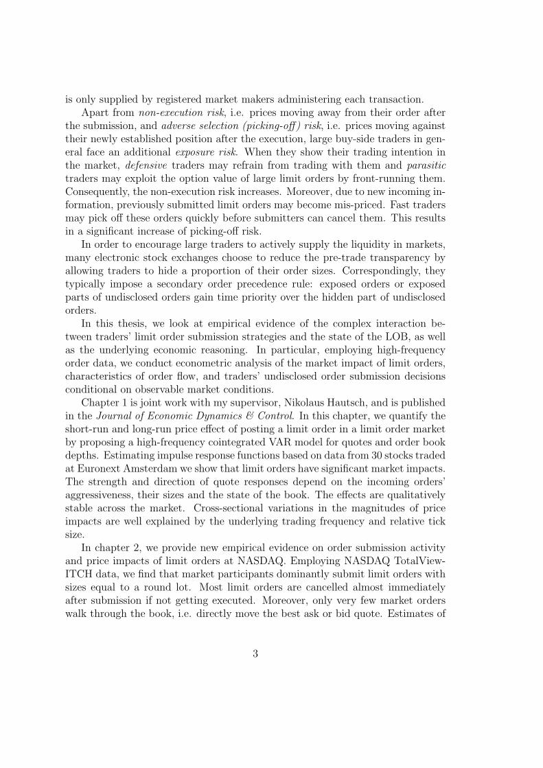
is only supplied by registered market makers administering each transaction.Apart from non-execution risk, i.e. prices moving away from their order after
the submission, and adverse selection (picking-off) risk, i.e. prices moving againsttheir newly established position after the execution, large buy-side traders in gen-eral face an additional exposure risk. When they show their trading intention inthe market, defensive traders may refrain from trading with them and parasitictraders may exploit the option value of large limit orders by front-running them.Consequently, the non-execution risk increases. Moreover, due to new incoming in-formation, previously submitted limit orders may become mis-priced. Fast tradersmay pick off these orders quickly before submitters can cancel them. This resultsin a significant increase of picking-off risk.
In order to encourage large traders to actively supply the liquidity in markets,many electronic stock exchanges choose to reduce the pre-trade transparency byallowing traders to hide a proportion of their order sizes. Correspondingly, theytypically impose a secondary order precedence rule: exposed orders or exposedparts of undisclosed orders gain time priority over the hidden part of undisclosedorders.
In this thesis, we look at empirical evidence of the complex interaction be-tween traders’ limit order submission strategies and the state of the LOB, as wellas the underlying economic reasoning. In particular, employing high-frequencyorder data, we conduct econometric analysis of the market impact of limit orders,characteristics of order flow, and traders’ undisclosed order submission decisionsconditional on observable market conditions.
Chapter 1 is joint work with my supervisor, Nikolaus Hautsch, and is publishedin the Journal of Economic Dynamics & Control. In this chapter, we quantify theshort-run and long-run price effect of posting a limit order in a limit order marketby proposing a high-frequency cointegrated VAR model for quotes and order bookdepths. Estimating impulse response functions based on data from 30 stocks tradedat Euronext Amsterdam we show that limit orders have significant market impacts.The strength and direction of quote responses depend on the incoming orders’aggressiveness, their sizes and the state of the book. The effects are qualitativelystable across the market. Cross-sectional variations in the magnitudes of priceimpacts are well explained by the underlying trading frequency and relative ticksize.
In chapter 2, we provide new empirical evidence on order submission activityand price impacts of limit orders at NASDAQ. Employing NASDAQ TotalView-ITCH data, we find that market participants dominantly submit limit orders withsizes equal to a round lot. Most limit orders are cancelled almost immediatelyafter submission if not getting executed. Moreover, only very few market orderswalk through the book, i.e. directly move the best ask or bid quote. Estimates of
3

impulse-response functions on the basis of a cointegrated VAR model for quotesand market depths allow us to quantify the market impact of incoming limit orders.We propose a method to predict the optimal size of a limit order conditional onits position in the book and a given fixed level of expected market impact. Thischapter is joint work with Nikolaus Hautsch and is published on the conferenceproceeding of “Market Microstructure, Confronting Many Viewpoints”.
Trading under limited pre-trade transparency becomes increasingly popularon financial markets. In Chapter 3, we provide first evidence on traders’ use of(completely) undisclosed orders in electronic trading. Employing TotalView-ITCHdata on order messages at NASDAQ, we propose a simple method to conduct sta-tistical inference on the location of hidden depth given the state of the market.We show that market conditions reflected by the bid-ask spread, (visible) depth,recent price movements and trading signals affect traders’ decisions where to posthidden orders. Our evidence suggests that traders optimize their hidden orderplacements to (i) compete for the provision of (hidden) liquidity and (ii) protectthemselves against adverse selection, front-running as well as “hidden order de-tection strategies” used by high-frequency traders. Overall, our results show thathidden liquidity is predictable given observable market characteristics and is a keyelement in modern trading and execution strategies. This chapter is joint workwith Nikolaus Hautsch.
The rise of algorithmic trading in electronic limit order markets creates consid-erable challenges for researchers, who have to cope with extremely large amountsof trading data produced daily by exchanges. In chapter 4, we present a pro-gram framework for reconstructing LOBs as well as extracting order flow infor-mation from message stream data. The system is modularized based on commonorder events in the generalized order-processing of limit order markets, so thatit can be easily adapted to data from any limit order markets. Moreover, theunderlying data structures in the basic modules are highly optimized and algo-rithms are exhaustively tested to guarantee the reliability of the output data andthe efficiency of the entire system. This chapter is joint work with my colleagueTomas Polak, and a software treating the NASDAQ TotalView-ITCH data is im-plemented by the LOBSTER development team and is accessible for all researchersvia http://lobster.wiwi.hu-berlin.de.
4

Chapter 1
Market Impact of a Limit Order
This chapter is based on Hautsch and Huang (2012b).
1.1 Introduction
It is well known that the revelation of trading intention adversely affects asset prices.As also confirmed by theoretical studies1, passive order placement through limit ordersincurs significant market impact even if the order is not been executed. In financialpractice, the risk to ‘scare’ and to ultimately shift the market by limit order placementsis well-known and is taken into account in trading strategies. As a consequence, liquidityprovision through hidden orders, which allow traders to partly (or entirely) concealorder volume, has gained popularity. However, despite the importance of limit orderstrategies in modern trading, the actual impact of an incoming (visible) limit order onthe subsequent price process is still hardly explored and quantified. In fact, while theanalysis of the price impact resulting from a trade is a classical topic in traditional marketmicrostructure research (see, e.g., Dufour and Engle, 2000; Engle and Patton, 2004;Hasbrouck, 1991), empirical evidence on the market impact of limit order placements isaddressed by only few recent studies as Eisler, Bouchaud, and Kockelkoren (2011) andCont, Kukanov, and Stoikov (2011).
This chapter aims at filling this gap in the literature and addresses the followingempirical research questions: (i) How strong is the short-run and long-run impact of anincoming limit order in dependence of its position in the book, its size and the state of thebook? (ii) Are ask and bid quote responses to incoming limit orders widely symmetricor is there evidence for an asymmetric re-balancing of the book? (iii) How different isthe market impact of a limit order compared to that caused by a trade of similar size?(iv) How stable are these effects across the market and do they depend on stock-specificcharacteristics, such as the underlying trading intensity, minimum tick size and averagetrade size?
1See, e.g., Parlour and Seppi (2008), Boulatov and George (2008) and Rosu (2010).
5

We propose modelling the processes of ask and bid quotes as well as several levels ofdepth volume on both sides of the market in terms of a cointegrated vector autoregressive(VAR) model. This framework allows us to study the price impact of limit ordersby means of impulse response functions. Each limit order is represented by a shockdisturbing the multivariate system of quotes and depths and influencing it dynamicallyover time. Designing the shock vectors in a specific way allows us to characterize thetype of the limit order represented by its size and its position in the order queue as wellas the current state of the book.
The motivation for using a cointegrating system stems from the fact that ask and bidquotes are naturally integrated and tend to move in locksteps. Cointegration analysisreveals a stationary linear combination of bid and ask quotes which closely resembles thebid-ask spread. The idea of jointly modelling ask and bid quote dynamics in terms of acointegrated system originates from Engle and Patton (2004) based on the work of Has-brouck (1991) and has been used in other approaches, such as Hansen and Lunde (2006)and Escribano and Pascual (2006). Our setting extends and modifies this approach intwo major directions: Firstly, we model quotes and depth simultaneously. This yields anovel type of order book model capturing not only quote and depth dynamics but im-plicitly also dynamics of midquotes, midquote returns, spreads, spread changes as wellas order book imbalances. Secondly, we model the system not only on a trade-to-tradebasis but exploit the complete order arrival process. Therefore, the model captures allrelevant trading characteristics in a limit order book market and thus provides a com-plete description of the order book in a range close to the best quotes. Hence, the modelis particularly useful for liquid assets where most of the market activity is concentratedat the best quote levels. In this sense, the approach complements dynamic models fororder book curves such as proposed by Hardle, Hautsch, and Mihoci (2009) and Russelland Kim (2010).
The proposed quote and depth model is estimated by Johansen’s (1991) full informa-tion maximum likelihood estimator using high-frequency order book data for 30 stockstraded on Euronext Amsterdam covering a sample period over two months in 2008.We find strong evidence for the existence of common stochastic components in quotesand corresponding depths resulting in cointegration relations which significantly deviatefrom the bid-ask spread. In this sense, our results shed some light on the strength ofco-movements in ask and bid prices depending on the underlying depth. Indeed, it turnsout that order book inventory is highly persistent and reveals high-frequency dynamicsresembling (near-)unit-root behavior. We show that incoming limit orders have signif-icant impacts on subsequent ask and bid processes. It turns out that the magnitudeand direction of quote adjustments strongly depend on the order’s aggressiveness, its(relative) size and the prevailing depth in the book. In particular, we show the followingresults: (i) Quote adjustments are the stronger and the faster, the closer the incomingorder is posted to the market. Most significant effects are reported for orders postedon up to two levels behind the market. For less aggressive orders, virtually no effectscan be quantified. (ii) Limit orders temporarily narrow the spread. Converse effects areshown for market orders. In the long-run, these effects are reverted back in an asym-
6

metric way. (iii) Large limit orders posted inside of the spread induce severe long-runeffects pushing the market in the intended trading direction. In contrast, small limitorders posted inside of the spread tend to be picked up quickly inducing adverse pricereactions. (iv) The long run market impact of aggressive market orders walking throughthe book is the higher the smaller the prevailing depth behind the market. (v) The ef-fects are qualitatively stable across the market, where the absolute magnitudes of priceimpacts differ in dependence of underlying stock-specific characteristics. It turns outthat approximately 60%-80% of the cross-sectional variation in market impacts can beexplained by the trading frequency and the minimum tick size.
The remainder of this chapter is structured as follows. In Section 1.2, we describethe trading structure of Euronext Amsterdam and provide descriptive statistics. Theeconometric approach is explained in Section 1.3. Section 1.4 gives the estimation resultsand Section 1.5 provides the quantified price impacts of different types of limit orders.Finally, Section 1.6 concludes.
1.2 Data and Market Environment
Euronext is a purely electric limit order book market with price and time order prece-dence. During the continuous trading period between 9:00 and 17:30 CET, limit ordersare submitted to a centralized computer system where they are matched to prevailingstanding limit orders on the opposite side. If there is no match or the matched volumein the system is insufficient to exhaust the incoming order, the remaining order volumeis placed in the order book. Euronext supports various order types like pure marketorders (immediate order execution without a price limit), stop orders (automatic issuingof limit orders or market orders when a given price is reached), fill-or-kill (FOK) ordersor iceberg orders.
Our dataset comprises limit order book (LOB) data of the 30 most frequently tradedstocks at Euronext Amsterdam between August 1st and September 30th, 2008. Since onSeptember 1st, Euronext changed the minimum tick size for some stocks, we analyze thetwo months August and September separately. This allows us to study the robustnessof our findings under changing market conditions. Since these two months represent agenerally turbulent market period, we further robustify our findings by replicating ouranalysis for a period which is less volatile. As we obtain quantitatively similar results,our findings can be seen as representative for different market conditions.2
The data contains information on the prevailing market depth (in terms of the num-ber of shares) for the five best quotes on both sides of the market. Every trade andchange of the order book are recorded in milliseconds. Preliminary analyzes (which arealso supported by the findings given in Section 1.5) show that aggressive limit ordersplaced close to the best ask and bid have the highest market impact while induced priceeffects significantly decline with the distance to the spread. Accordingly, we focus only
2These results are not shown in this chapter but are available on our web appendix or uponrequest.
7

on the best three price levels in the book. Unlike the trade data which is well filteredby built-in filters in the database3, the order book data is completely raw. We removeobservations where (i) the spread is zero or negative, and (ii) ask or bid quotes changeby more than 2%.4 Moreover, to remove effects due to the opening and closing of themarket, we discard data of the first five and last five minutes of the continuous tradingperiod.
Matching of trade and LOB data is achieved by a matching algorithm which isdescribed in details in Appendix A.1. This algorithm matches a trade with the corre-sponding LOB observation by comparing its price and volume with the resulting changesof quotes and depths in the book within an adaptively chosen time window. It minimizesthe probability of misclassifications and as a by-product provides an estimate of the timeasynchronicity between trade and LOB records.5 To classify the initiation type of trades,we use a hybrid procedure according to Lee and Ready (1991). Firstly, we determinethe type of trades which are located in more than one second time distance to previoustrades using the mid-quote method. I.e., if a trade occurs with a price greater (less) thanthe most current mid-quote, it is classified as a buy (sell). If the trade price equals themid-quote, it is marked as ‘undetermined’. Secondly, ‘undetermined’ trades and tradeswhich follow previous trades in less than one second time distance are classified by thetick-test method. Accordingly, if the trade price is higher (lower) than the previous one,it is identified as a buy (sell). If it does not change the price, it is categorized as thesame type as the previous one. Finally, we identify sub-trades arising from the executionof a big market order against several (smaller) limit orders if they occur in less than onesecond after the previous trade and have the same initiation types. All correspondingsub-trades are consolidated to a single trade.
Table 1.1 gives descriptive statistics of the resulting August data used in this chap-ter.6 We observe significantly more limit order activities than market orders. Theaverage bid-ask spread is decreasing with the liquidity of the underlying stock. On aver-age, second level market depth is higher than first level depth while it is approximatelyequal to the depth on the third level.
3Besides recording errors, block trades and trades in auction periods are excluded.4In order to limit the volatility, Euronext NSC suspends continuous trading if prices change
by more than 2%. This is not exactly the same rule as that implemented here, but it is reasonablymimicked.
5Due to technological progress in the last decades, the time delay between trade and quoterecords is nowadays hardly greater than one second. Consequently, the ‘five-second’ rule accord-ing to Lee and Ready (1991), which has been commonly used in empirical market microstructureliterature, is not appropriate anymore for more recent datasets.
6Due to the aforementioned change in the minimum tick size, it is not appropriate to presentjoint summary statistics for both months. However, as the descriptive statistics for Septemberare very similar to that for August, we do not present them here.
8

Table 1.1Summary of synchronized trade and order book data.The sample consists of the 30 most frequently traded stocks on Euronext Amsterdam. Market depth is measured in
thousand shares. L1-L3 denote the order book level one to three. The period is from 1st to 31st August 2008.
stocks #trades #LO activ. Ask Bid Mean of ask depth Mean of bid depthper day per day min mean max min mean max L1 L2 L3 L1 L2 L3
ING 1606.8 66569.1 20.255 21.518 23.290 20.250 21.507 23.275 3.64 3.94 4.12 3.45 3.90 4.14FOR 1304.6 27574.0 8.770 9.351 10.160 8.760 9.338 10.150 16.78 25.76 25.03 16.35 26.25 24.20RDSa 1166.2 48630.6 21.900 22.991 23.935 21.890 22.981 23.930 4.30 5.21 5.80 4.00 5.06 5.59UNc 1152.1 46023.7 17.110 18.635 19.670 17.100 18.625 19.660 4.76 5.24 6.44 4.52 5.33 6.49
AHLN 1119.4 18730.3 7.540 8.510 8.970 7.530 8.502 8.960 7.89 9.80 10.23 8.18 10.64 10.59PHG 1108.3 34722.0 20.875 22.381 23.465 20.870 22.368 23.450 2.18 2.36 2.70 1.95 2.19 2.59
AEGN 982.5 43270.2 7.290 7.909 8.400 7.280 7.902 8.395 5.12 4.99 4.86 4.98 4.98 4.79AKZO 960.0 20061.2 35.460 39.571 41.920 35.400 39.541 41.910 0.89 0.96 1.00 0.78 0.90 0.98KPN 954.0 20733.8 10.915 11.274 11.680 10.905 11.266 11.670 9.61 12.10 12.77 8.79 10.57 11.57TNT 949.7 20412.7 22.040 24.598 27.000 22.030 24.566 26.970 1.57 1.91 2.15 1.51 1.96 2.24HEIN 927.2 19782.1 29.540 31.796 33.660 29.520 31.767 33.600 0.98 1.10 1.13 0.92 1.00 1.04ISPA 903.1 35708.2 49.990 52.694 56.440 49.910 52.661 56.420 1.85 2.76 3.66 1.97 3.08 3.84
ASML 853.8 26249.5 14.290 15.964 17.400 14.280 15.949 17.390 3.80 5.86 6.50 3.48 5.21 6.01DSMN 826.7 21574.5 36.050 37.919 40.000 36.020 37.886 39.990 0.77 0.87 0.99 0.77 0.88 0.99SBMO 603.7 18676.3 13.530 14.934 16.700 13.520 14.911 16.680 1.84 2.63 2.99 1.76 2.51 2.79TOM2 505.3 16822.0 14.340 16.017 17.550 14.300 15.987 17.540 1.31 1.71 2.06 1.25 1.69 1.75FUGRc 505.0 8846.5 43.620 47.701 53.200 43.610 47.631 53.180 0.56 0.54 0.52 0.49 0.49 0.47WLSNc 548.8 16003.6 14.610 15.973 17.020 14.550 15.950 17.000 1.92 1.88 1.96 1.94 1.83 1.89RAND 543.4 17265.2 17.710 19.432 21.430 17.690 19.397 21.400 1.09 1.56 1.75 1.07 1.47 1.47ELSN 488.5 29702.2 10.390 11.049 11.510 10.350 11.035 11.500 7.27 11.57 11.96 6.81 11.34 12.44BOSN 419.6 8013.0 32.320 36.323 41.900 32.250 36.247 41.890 0.52 0.52 0.49 0.53 0.51 0.47BAMN 416.8 6334.1 9.900 10.736 12.220 9.860 10.714 12.200 2.06 2.35 2.38 1.99 2.25 2.19
SR 347.5 6396.6 10.370 11.588 13.200 10.360 11.563 13.180 1.70 1.80 1.76 1.72 1.71 1.48CSMNc 340.2 7478.4 17.910 20.395 24.260 17.890 20.361 24.240 0.81 0.88 0.92 0.84 0.90 0.91
COR 327.1 12103.2 47.090 49.273 51.210 47.010 49.175 51.140 0.43 0.41 0.37 0.39 0.38 0.34IMUN 292.7 5735.9 14.300 16.178 17.710 14.280 16.148 17.700 0.92 1.17 1.24 0.85 0.91 0.88
SMTNc 272.4 7648.8 43.920 52.282 60.440 43.840 52.112 60.300 0.22 0.25 0.22 0.26 0.27 0.26NUTR 256.6 8043.2 41.160 43.275 44.900 41.120 43.192 44.890 0.40 0.36 0.33 0.37 0.38 0.38USGP 248.5 6342.3 9.670 11.198 12.630 9.650 11.168 12.600 1.47 1.51 1.41 1.59 1.39 1.19HEIO 181.0 14011.0 27.120 29.854 31.300 27.080 29.809 31.290 0.44 0.53 0.61 0.50 0.64 0.70
9
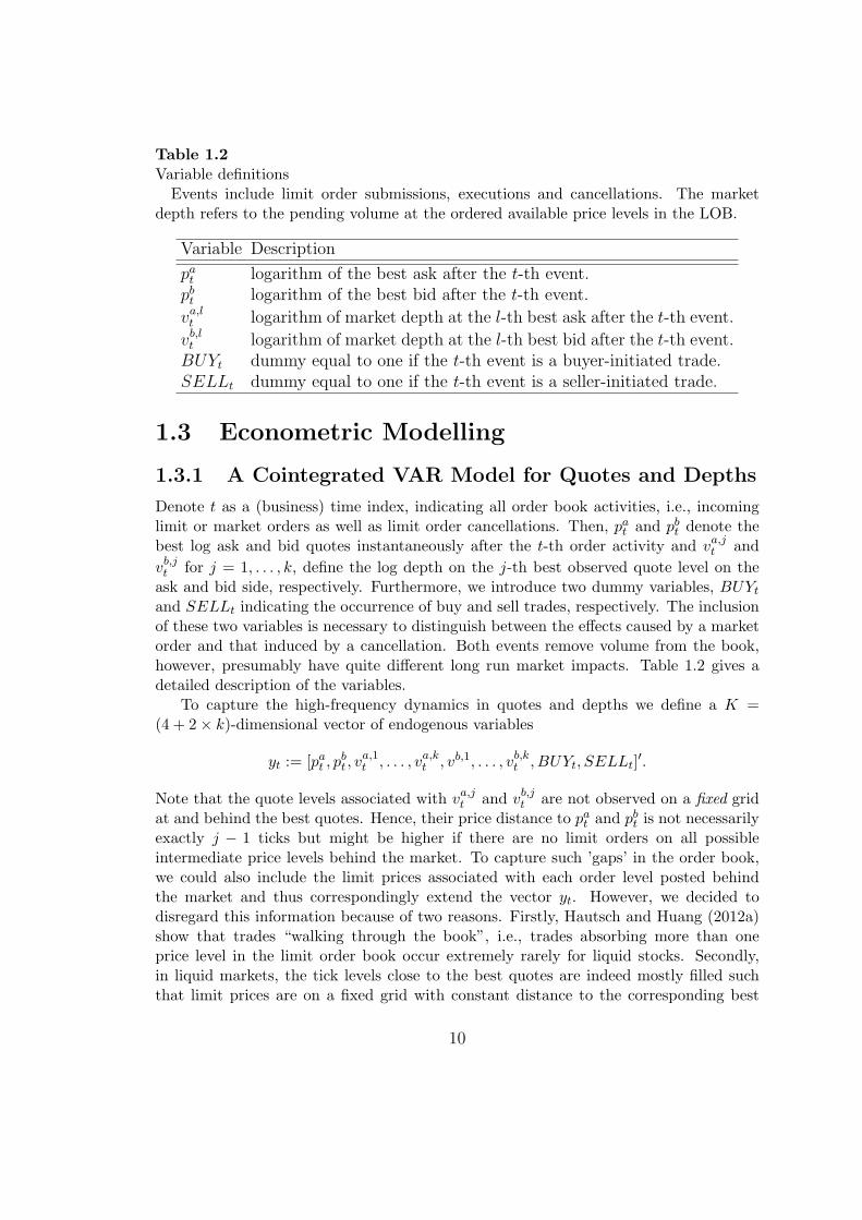
Table 1.2Variable definitionsEvents include limit order submissions, executions and cancellations. The market
depth refers to the pending volume at the ordered available price levels in the LOB.
Variable Description
pat logarithm of the best ask after the t-th event.pbt logarithm of the best bid after the t-th event.
va,lt logarithm of market depth at the l-th best ask after the t-th event.
vb,lt logarithm of market depth at the l-th best bid after the t-th event.BUYt dummy equal to one if the t-th event is a buyer-initiated trade.SELLt dummy equal to one if the t-th event is a seller-initiated trade.
1.3 Econometric Modelling
1.3.1 A Cointegrated VAR Model for Quotes and Depths
Denote t as a (business) time index, indicating all order book activities, i.e., incominglimit or market orders as well as limit order cancellations. Then, pat and pbt denote thebest log ask and bid quotes instantaneously after the t-th order activity and va,jt and
vb,jt for j = 1, . . . , k, define the log depth on the j-th best observed quote level on theask and bid side, respectively. Furthermore, we introduce two dummy variables, BUYtand SELLt indicating the occurrence of buy and sell trades, respectively. The inclusionof these two variables is necessary to distinguish between the effects caused by a marketorder and that induced by a cancellation. Both events remove volume from the book,however, presumably have quite different long run market impacts. Table 1.2 gives adetailed description of the variables.
To capture the high-frequency dynamics in quotes and depths we define a K =(4 + 2× k)-dimensional vector of endogenous variables
yt := [pat , pbt , v
a,1t , . . . , va,kt , vb,1, . . . , vb,kt , BUYt, SELLt]
′.
Note that the quote levels associated with va,jt and vb,jt are not observed on a fixed gridat and behind the best quotes. Hence, their price distance to pat and pbt is not necessarilyexactly j − 1 ticks but might be higher if there are no limit orders on all possibleintermediate price levels behind the market. To capture such ’gaps’ in the order book,we could also include the limit prices associated with each order level posted behindthe market and thus correspondingly extend the vector yt. However, we decided todisregard this information because of two reasons. Firstly, Hautsch and Huang (2012a)show that trades “walking through the book”, i.e., trades absorbing more than oneprice level in the limit order book occur extremely rarely for liquid stocks. Secondly,in liquid markets, the tick levels close to the best quotes are indeed mostly filled suchthat limit prices are on a fixed grid with constant distance to the corresponding best
10

quotes. Consequently, we expect that the inclusion of all individual limit prices doesnot provide any additional information but just increases the dimension of the system.Finally, modelling log volumes instead of plain volumes is a common practice in manyempirical studies to reduce the impact of extraordinarily large volumes. This is alsosuggested by Potters and Bouchaud (2003) studying the statistical properties of marketimpacts of trades. Moreover, using logs implies that changes in market depth can beinterpreted as relative changes with respect to the current depth level.
Hence, we model log quotes, log depths and trading indicators as a restricted coin-tegrated vector autoregressive model of the order p (VAR(p)) with the vector errorcorrection (VEC) form
∆yt = µ+ αβ′yt−1 +
p−1∑
i=1
Γi∆yt−i + ut, (1.1)
where ut is white noise with covariance matrix Σu, µ is a constant, Γi with i = 1, . . . , p−1is a K × K parameter matrix, α and β denote the K × r loading and cointegratingmatrices with r < K. As we can safely assume that the trading indicators BUYt andSELLt are stationary, we restrict the two first columns of β as β1 = [0, . . . , 0, 1, 0]′ andβ2 = [0, . . . , 0, 0, 1]′.
For the impulse-response analysis below, it turns out to be more convenient to workwith the reduced VAR representation in terms of the level of yt,
yt = µ+
p∑
i=1
Aiyt−i + ut, (1.2)
where A1 := IK + αβ′ + Γ1 with IK denoting a K ×K identity matrix, Ai := Γi − Γi−1
with 1 < i < p and Ap := −Γp−1.We estimate the model (1.1) by the Full Information Maximum Likelihood (FIML)
estimator proposed by Johansen (1991) and Johansen and Juselius (1990). Then, fol-lowing Lutkepohl and Reimers (1992), we transform these estimates to representation(1.2). The corresponding procedure is shown in Appendix A.2 and A.3. By imposingthe stationarity restrictions β1 and β2, all elements in the other cointegrating vectorsassociated with BUYt and SELLt are automatically set to zero. This is guaranteed bythe orthogonality among the estimated cointegrating vectors implied by FIML.
Note that market depth enters the vector yt in levels and thus is treated as a possi-bly non-stationary variable. Though this is counter-intuitive for the behavior of depthover longer horizons, it is a reasonable assumption if depth is observed on very highfrequencies. Moreover, modelling both quotes and depth in terms of a cointegrationsystem guarantees consistency of parameter estimates irrespective of the possible (non-)stationarity of order book depth. Even if depth is truly stationary (and thus justcorresponds to a (spurious) cointegration relation for itself), FIML estimates are consis-tent (though obviously not efficient).7 Since we employ a high number of observations,
7See, for instance, Example 3.1 in Johansen (1995) for an illustration of this argument.
11

the possible loss of efficiency due to the neglect of a (stationarity) restriction is notvery harmful in our context. If, however, we impose stationarity of depth and corre-spondingly restrict the cointegration vectors, we run the risk of producing inconsistentestimates if the restriction does not hold. Indeed, unit root tests applied in Section 1.4.1indicate that the assumption of a unit root in depth observed on high frequencies cannotbe rejected for many stocks. These arguments support the usefulness of a more robuststatistical inference in form of an unrestricted cointegration system.
Model (1.2) can be further rotated in order to represent dynamics in spreads, relativespread changes, midquotes, midquote returns as well as (ask-bid) depth imbalances.Hence, the model is sufficiently flexible to capture the high-frequency dynamics of allrelevant trading variables.8
Finally, in models involving only quote dynamics (e.g. Engle and Patton, 2004) orspread dynamics (e.g. Lo and Sapp, 2006), the error correction term β′yt is typicallyassumed to be equal to the spread implying a linear restriction R′β = 0 with R′ =[1, 1, 0, . . . , 0]. However, given the potential non-stationarity of order book depth, we donot impose this assumption here. As depth might contain information on the equilibrium(long run) state of the order book as well, we expect the existence of cointegrationrelations differing from spreads and involving both quotes and depths. As shown in theremainder of this chapter, this notion is actually supported by the data.
1.3.2 Limit Orders as Shocks to the System
In this section, we illustrate how to represent incoming orders as shocks to the systemspecified in equation (1.2). Whenever an order enters the order book, it (i) will changethe depth in the book, (ii) may change the best quotes depending on which position inthe queue it is placed, and (iii) will change the trading indicator dummy in case of amarket order. We represent these changes in terms of an impulse vector δ := [δ′v, δ
′p, δ
′d]′
with δv being a 2k × 1 vector associated with shocks to the depths, δp denoting a 2× 1vector consisting of shocks to the quotes and δd being a 2× 1 vector representing shocksto the trading indicator dummy.
We design impulse response vectors associated with five scenarios commonly facedby market participants. As graphically illustrated by Figures 1.1 to 1.4, a three-levelorder book is initialized by the best ask pat = 1002, best bid pbt = 1000, second best ask1003, second best bid 999, and levels of depths on the bid side V b,1
t = 1, V b,2t = 1.5,
V b,3t = V b,4
t = 1.4. The following scenarios are considered:9
Scenario 1a (normal limit order): Arrival of a buy limit order with price 1000 andsize 0.5 to be placed at the market. As shown in Figure 1.1, this order will be
8Note that we do not impose an explicit constraint ensuring the positiveness of bid-ask spreads.As shown on the companion website, this restriction is implicitly satisfied by our estimates invirtually all cases.
9For sake of brevity, the scenarios are only characterized for buy orders. For sell orders, thesetting is correspondingly adapted to the other side of the market.
12

1
1.51.4
1
1.51.4
price
depth
0.5
⇒1
1.51.4
1.51.51.4
pricedepth
Figure 1.1 (Scenario 1a (normal limit order)): An incoming buy limit order withprice 1000 and size 0.5. It affects only the depth at the best bid without changing theprevailing quotes or resulting in a trade.
1
1.51.4
1
1.51.4
price
dep
th
0.5
⇒1
1.51.4
1
1.5
0.5
price
dep
th
Figure 1.2 (Scenario 2 (aggressive limit order)): An incoming buy limit orderwith price 1001 and size 0.5 improving the best bid and changing all depth levels on thebid side of the order book.
13
1
1.51.4
1
1.51.4
price
depth
0.5
⇒ 0.5
1.51.4
1
1.51.4
price
depth
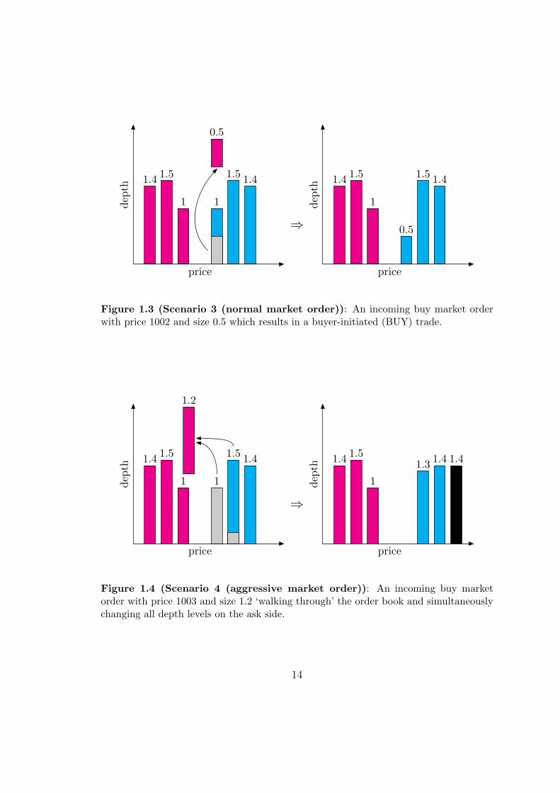
Figure 1.3 (Scenario 3 (normal market order)): An incoming buy market orderwith price 1002 and size 0.5 which results in a buyer-initiated (BUY) trade.
1.51.4
11
1.51.4
price
dep
th
1.2
⇒
1.31.4 1.4
1
1.51.4
price
dep
th
Figure 1.4 (Scenario 4 (aggressive market order)): An incoming buy marketorder with price 1003 and size 1.2 ‘walking through’ the order book and simultaneouslychanging all depth levels on the ask side.
14
consolidated at the best bid without changing the prevailing quotes. Because theinitial depth on the first level is 1.0, the change of the log depth is ln(1.5) ≈ 0.4.Correspondingly, the shock vectors are given by δv = [0, 0, 0, 0.4, 0, 0]′, δp = δd =[0, 0]′.
Scenario 1b (passive limit order): Arrival of a buy limit order with price 999 andsize 0.5 to be posted behind the market. As in the scenario above, it does notchange the prevailing quotes and only affects the depth at the second best bid.We have δv = [0, 0, 0, 0, ln(2)− ln(1.5) ≈ 0.29, 0]′, δp = δd = [0, 0]′.
Scenario 2 (aggressive limit order): Arrival of a buy limit order with price 1001and size 0.5 to be posted inside of the current spread. Figure 1.2 shows that it im-proves the best bid by 0.1% and accordingly shifts all depth levels on the bid side.The resulting shock vector is given by δv = [0, 0, 0, (ln(0.5) ≈ −0.69), (ln(1/1.5) ≈−0.4), (ln(1.5/1.4) ≈ 0.07)]′, δp = [0, 0.001]′ and δd = [0, 0]′.
Scenario 3 (normal market order): Arrival of a buy order with price 1002 and size0.5. This order will be executed immediately against standing limit orders at thebest ask. Because it absorbs liquidity from the book, it shocks the correspondingdepth levels negatively. Figure 1.3 depicts the corresponding changes of the orderbook as represented by δv = [ln(0.5) ≈ −0.69, 0, 0, 0, 0, 0]′, δp = [0, 0]′ and δd =[1, 0]′.
Scenario 4 (aggressive market order): Arrival of a buy order with price 1003 andsize 1.2. It ‘walks up’ the order book. As shown in Figure 1.4, the best askquote and all depth levels are simultaneously shifted resulting in the shock vectorδv = [(ln(1.3) ≈ 0.26), (ln(1.4/1.5) ≈ −0.07), 0, 0, 0, 0]′, δp = [(1/1002) ≈ 0.001, 0]′
and δd = [1, 0]′.
Table 1.3 summarizes the shock vectors implied by the illustrated scenarios.
1.3.3 Measuring the Market Impact
We quantify the market impact of limit orders as the implied expected short-run andlong-run shifts of the ask and bid after their submissions. This reaction is captured bythe impulse response function,
f(h; δy) = E[yt+h|yt + δy, yt−1, · · · ]− E[yt+h|yt, yt−1, · · · ], (1.3)
where the shock on quotes, depths and trading indicators is denoted by δy := [δ′p, δ′v, δ
′d]′
and h is the number of periods (measured in ‘order event time’).Note that we do not have to orthogonalize the impulse since contemporaneous rela-
tionships between quotes and depths are captured by construction of the shock vector.Moreover, our data is based on the arrival time of orders avoiding time aggregation asanother source of mutual dependence in high-frequency order book data.
15

Table 1.3Shock vectors implied by the underlying five scenariosInitial order book: best ask pat = 1002, best bid pbt = 1000, second best ask = 1003,
second best bid = 999. Volumes on the ask/bid side: Va/b,1t = 1 at the best bid,
Va/b,2t = 1.5 at the second best bid, and V
a/b,3t = V
a/b,4t = 1.4 at the third and fourth
best bids, respectively. Notation: δv denotes shocks on market depths; δp denotes shockson the best bid and best ask; δd denotes shocks on trading indicator variables.
Scenario limit order shock vectors(dir,price,size) δ′v δ′p δ′d
‘normal limit order’ (Bid,1000, 0.5) [0, 0, 0, 0.4, 0, 0] [0, 0] [0, 0]‘passive limit order’ (Bid,999, 0.5) [0, 0, 0, 0, 0.29, 0] [0, 0] [0, 0]‘aggressive limit order’ (Bid,1001, 0.5) [0, 0, 0,−0.69,−0.4, 0.07] [0, 0.001] [0, 0]‘normal market order’ (Bid,1002, 0.5) [−0.69, 0, 0, 0, 0, 0] [0, 0] [1, 0]‘aggressive market order’ (Bid,1003, 1.2) [0.26,−0.07, 0, 0, 0, 0] [0.001, 0] [1, 0]
Using impulse-response analysis to retrieve the market impact has two major advan-tages. First, in contrast to an analysis of estimated VEC coefficients which only revealsthe immediate impact, it enables us to examine both long-run and short-run effects. Sec-ond, it allows us to straightforwardly quantify the joint effect induced by simultaneouschanges of several variables given a certain state of other variables.
We consider two moving average (MA) representations of the cointegrated VARmodel. The first one is based on the reduced form given by equation (1.2). This repre-sentation allows us to compute the path of the response function over time. The secondone is the Granger representation based on the VECM form in equation (1.1) whichenables us to explicitly compute the permanent (long-run) response.
We start our discussion with the first MA representation. The companion VAR(1)form of the VAR(p) model in equation (1.2) is given by
Yt = µ+AYt−1 + Ut, (1.4)
where
µ :=
µ0...0
︸︷︷︸Kp×1
, Yt :=
ytyt−1...
yt−p+1
︸ ︷︷ ︸Kp×1
, Ut :=
ut0...0
︸ ︷︷ ︸Kp×1
16

and
A :=
A1 · · · Ap−1 Ap
IK 0 0. . .
......
0 · · · IK 0
︸ ︷︷ ︸Kp×Kp
.
Successively substituting Y yields
Yt = Mt +t−1∑
i=0
AiUt−i, (1.5)
where Mt = AtY0 +∑t
i=0Aiµ consists of terms of an initial value and a deterministic
trend, which are irrelevant for the impulse-response analysis. Let J := [IK : 0 : · · · : 0]be a K × Kp selection matrix with JYt = yt. Pre-multiplying J on both sides ofequation (1.5) and using Ut = J ′ut gives
yt = JMt +t−1∑
i=0
JAiJ ′ut−i. (1.6)
Then, the linear impulse-response function according to equation (1.3) can be writtenas
f(h; δy) = JAhJ ′δy. (1.7)
Given the consistent estimator a for a := vec(A1, . . . , Ap) in equation (1.2),
√T (a− a)
d→ N (0,Σa),
Lutkepohl (1990) shows that the asymptotic distribution of the impulse-response func-tion is given by √
T (f − f)d→ N (0, GhΣaG
′h), (1.8)
where Gh := ∂ vec(f)/∂ vec(A1, · · · , Ap)′. This expression can be explicitly written as
Gh =h−1∑
i=0
(δ′yJ(A
′)h−1−i⊗ JAiJ ′
). (1.9)
In order to compute the long-run effect, we apply Granger’s Representation Theoremto model (1.1) yielding
yt = Ct∑
i=1
(ui + µ) + C1(L) (ut + µ) + V, (1.10)
where
C = β⊥
(α′⊥
(IK −
p−1∑
i=1
Γi
)β⊥
)−1
α′⊥ . (1.11)
17

Here, L is the lag operator and the power series C1(z) is convergent for |z| < 1 + ξ forsome ξ > 0. V depends on initial values, such that β′V = 0. The Granger representationdecomposes the cointegrated process into a random walk term (C term), a stationaryprocess (C1 term) and a deterministic term (V ). Because of the convergence of the seriesC1(z), the response implied by this sub-process will be zero in the long run. Moreover,the deterministic term V is irrelevant for the impulse response. Therefore, the permanentresponse of the system is completely determined by the first term. Note that the shockδy causes this term changing by Cδy. Thus, we can express the permanent response as
f(δy) := limh→∞
f(h; δy) = Cδy. (1.12)
Note that given α and β, α⊥ and β⊥ are not uniquely identified. However, theright hand side of equation (1.11) is invariant with respect to the choice of these bases.Therefore, f(δy) is unique given the parameters and the shock vector in model (1.1).In practice, estimated responses and their covariances are obtained by replacing theunknown parameters in equation (1.7), (1.8) and (1.12) by their estimates.
1.4 Estimation Results
The underlying order book data contains bid and ask quotes as well as five levels of depth.Preliminary analyzes show that the depths on the fourth and fifth levels do not havesignificant effects on bid and ask quotes. Therefore, in our empirical study, we only usemarket depths up to the third level. In order to keep the analysis tractable, we reducethe computational burden induced by the high number of observations by separatelyestimating the model for each of the 43 trading days. This strategy allows us alsoto address possible structural changes, e.g., due to stock specific news announcementsor overnight effects. The market impact is then computed as the monthly average ofindividual (daily) impulse responses. Likewise, confidence intervals are computed basedon daily averages. To account for a structural break due to the change of the tick sizefor some stocks on September 1, 2008, we treat the two months August and Septemberseparately.
For sake of brevity we refrain from presenting all individual results for the 30analyzed stocks in this chapter. We rather illustrate the analyzed effects for thestock Fortis (FOR in Table 1.1) in August 2008. Fortis is one of the most activelytraded stocks and is representative for a major part of the market. The results forthe remaining stocks and the remaining periods are provided in a web appendix onhttp://amor.cms.hu-berlin.de/~huangrui/project/impact_of_orders. As shownin the web appendix and discussed in more detail in Section 1.5.5, the effects are quali-tatively remarkably similar across the market though the magnitudes of market impactsdiffer in dependence of underlying stock-specific characteristics.
The empirical analysis employs a VAR(15) specification which is selected based onresidual diagnostics and information criteria. Testing for serial correlation using theLjung-Box test according to Ljung and Box (1978) reveals almost no remaining serial
18

0 4000 8000 12000 16000 20000 24000 28000 32000 36000 40000−2
−1
0
1
2
3
4
5
Event time
Log
Dep
th
Ask level 1Ask level 3
Figure 1.5: Time series plot of log market depths (measured in thousand share units).Trading of Fortis, Euronext, Amsterdam, August 1st, 2008.
correlation in the residuals for all regressions based on a 1% level using ten lags. Thecorresponding statistics are also recorded in the web appendix.
1.4.1 Statistical Properties of Market Depth
Figure 1.5 provides time series plots of depths on the best ask and third best ask levelof the order book for a single (though representative) trading day for Fortis. A generalfinding is that the depth behind the market is typically greater than that at the market.Furthermore, there is evidence for co-movements between the individual depth levels,partially because of the ‘shift’ effect induced by aggressive orders, e.g., limit ordersposted inside of spreads or market orders completely absorbing the best price levels.
Figure 1.6 depicts the unconditional distributions and autocorrelation functions of logmarket depth. We observe that the distribution of depth behind the market is similar,though they are quite different from those at the market. The same pattern is alsoobserved for the autocorrelation functions. These empirical peculiarities are due to thefact that there is obviously more order activity at the market than behind the market.Consequently, market depth is more frequently changed at the best level inducing alower persistence than at higher levels. This might also explain why the unconditionaldistribution of depth is more dispersed than that of depth behind the market.
Table 1.4 shows the results of Augmented Dickey-Fuller (ADF) and KPSS tests forquotes and market depth. While the quote series are obviously integrated, we obtainconflictive findings for the depth series. The ADF tests reject the null hypothesis of aunit root in first level depth in 83% of all cases (across stocks and days), whereas the
19

−8 −6 −4 −2 0 2 4 60
0.1
0.2
0.3
0.4
0.5
0.6
0.7
0.8
0.9
Log Depth
dens
ity
Ask level 1Ask level 2Ask level 3
0 20 40 60 80 100 120 140 160 180 2000
0.1
0.2
0.3
0.4
0.5
0.6
0.7
0.8
0.9
1
lags
acf
Ask level 1Ask level 2Ask level 3
Figure 1.6: Left: Kernel density estimates of (log) market depths. Right: Auto-correlation functions of (log) market depths. Trading of Fortis, Euronext, Amsterdam,August 1st, 2008.
Table 1.4Stationarity tests on quotes and market depthsAugmented Dickey-Fuller (ADF) tests and KPSS tests for the 30 selected stocks on
each of the 43 trading days, i.e., 1290 time series for each variable. The chosen lag lengthis 50. The reported numbers are the sum of rejections at the 1%-level. In the ADF test,the null hypothesis is that there is an unit root in the process. In the KPSS test, thenull hypothesis is that there is no unit root in the process.
Variables pa pb va,1 va,2 va,3 vb,1 vb,2 vb,3
ADF 8 4 1072 975 933 1087 975 949(%) (0.62) (0.31) (83.1) (75.58) (72.32) (84.26) (75.58) (73.56)KPSS 1284 1283 871 905 982 846 896 979(%) (99.53) (99.45) (67.51) (70.15) (76.12) (65.58) (69.45) (75.89)
20

Table 1.5Representative estimates of cointegrating vectorsThe vectors are sorted according to their corresponding eigenvalues in Johansen’s ML
approach. The first two vectors are fixed to β1 = [0, . . . , 0, 1, 0] and β2 = [0, . . . , 0, 0, 1]representing stationary process of trading indicators. Correspondingly, all entries in β3to β9 associated with the trading indicator variables, BUY and SELL, are set to zeroand are omitted. Trading of Fortis at Euronext, Amesterdam on August 1, 2008.
Variable β3 β4 β5 β6 β7 β8 β9
pa -0.9987 -1.0000 1.0000 -0.9989 1.0000 -1.0000 0.9399pb 1.0000 0.9853 -0.9968 1.0000 -0.9767 0.7048 -1.0000
va,1 -0.0173 0.1629 -0.0416 0.0222 -0.0803 0.0919 -0.1039va,2 0.0070 -0.0486 0.0322 -0.0839 -0.1915 0.5869 -0.6605va,3 -0.0070 0.0140 -0.0212 0.0108 0.2980 0.6104 -0.5413vb,1 -0.0081 -0.1412 -0.0398 0.0827 -0.0442 -0.0807 -0.0933vb,2 0.0003 0.0527 0.0430 0.2321 0.0167 -0.8162 -0.4652vb,3 -0.0002 -0.0342 -0.0212 -0.2988 0.0796 -0.9414 -0.3337
KPSS tests reject the stationarity in 67% of all cases. For higher level depth, the evidenceagainst stationarity in depth is even higher. As discussed in Section 1.3.1, we explainthese findings by the fact that order book depth is an inventory variable which over shorthorizons is strongly autocorrelated and tend to behave like an I(1) process. On the otherhand, aggressive trading and limit order arrival create fluctuations in depth which areless predictable and reduce the strong persistence over longer intervals. Extreme changesarise, for instance, whenever first level depth is absorbed by an incoming order or, al-ternatively, is undercut by an incoming aggressive limit order, and thus the entire orderbook is shifted. Hence, from this discussion and the empirical findings we can concludethat depth might naturally contain stationary and non-stationary components where thelatter tend to dominate over very short horizons. Given these results, it is in any caserecommended to model depth as a non-stationary variable within a cointegrated VARframework. As discussed in Section 1.3.1, this proceeding ensures consistency of param-eter estimates even if depth might be stationary and, e.g., is fractionally cointegrated(see Johansen and Nielsen, 2010).
1.4.2 Estimated Cointegration Relations
For sake of brevity, we refrain from showing the individual estimates of A and B. Nev-ertheless, it is interesting to highlight the estimated cointegration relations. Accordingto Johansen’s trace statistics we identify seven cointegration relations among quotes anddepths. Table 1.5 shows the estimated cointegrating vectors for a representative trading
21

Table 1.6Representative estimates of the loading matrixValues in parentheses are t−statistics. Trading of Fortis at Euronext, Amesterdam on
August 1, 2008.
β3
′
yt−1 β4
′
yt−1 β5
′
yt−1 β6
′
yt−1 β7
′
yt−1 β8
′
yt−1 β7
′
yt−1
pat 0.0818 -0.0104 -0.0084 0.0042 0.0022 -0.0004 0.0002( 18.45) (-2.34) ( -50.11) ( 18.42) ( 8.50) (-2.65) ( 0.89)
pbt -0.0691 -0.0133 0.0026 0.0041 0.0007 -0.0004 -0.0000(-15.91) (-3.07) ( 15.58) ( 18.33) ( 2.77) (-2.59) (-0.07)
va,1t 2.1666 -0.4160 0.5319 0.0108 0.1228 0.0013 0.0052( 18.25) (-3.50) ( 118.70) ( 1.76) ( 17.52) ( 0.31) ( 0.75)
va,2t -0.2935 0.0512 -0.1776 0.0423 0.0995 -0.0074 0.0114( -7.44) ( 1.29) (-119.21) ( 20.65) ( 42.68) (-5.52) ( 5.01)
va,3t 0.0589 -0.0117 0.1293 -0.0176 -0.1314 -0.0072 0.0079( 1.58) (-0.31) ( 92.30) ( -9.14) (-59.94) (-5.72) ( 3.71)
vb,1t 1.5157 0.4704 0.7016 -0.1435 0.0596 0.0017 0.0025( 12.75) ( 3.96) ( 156.39) (-23.26) ( 8.49) ( 0.42) ( 0.37)
vb,2t -0.2284 -0.0607 -0.2373 -0.1053 -0.0036 0.0087 0.0074( -5.99) (-1.59) (-165.07) (-53.26) ( -1.58) ( 6.72) ( 3.40)
vb,3t -0.0492 0.0060 0.1322 0.1253 -0.0176 0.0119 0.0034( -1.39) ( 0.17) ( 99.52) ( 68.59) ( -8.44) (10.01) ( 1.66)
22

day, where we omit the two known cointegrating vectors associated with the (station-ary) trading indicators. Likewise we also omit the corresponding entries in the remainingcointegrating vectors as they are zero by construction. The resulting vectors are orderedaccording to their corresponding eigenvalues reflecting their likelihood contributions.Table 1.6 shows the estimated loading matrix, α, and corresponding t−statistics. Weobserve that not quotes but also depth variables have a significant loading on most ofthe six cointegration relations.
Figure 1.7 depicts the time series of the estimated cointegration relations. The seriesare quite different from that of the bid-ask spread (i.e., the difference between ask andbid quotes) which would be expected if depth does not belong to the cointegration vectorand is also depicted in the figure. Compared to the spread which reflects a very discretebehavior, the cointegration relations are much more smooth. Nevertheless, as any linearcombination of these vectors results into a further cointegration relation, it is required toformally test whether the estimated cointegration relations are indeed different from thebid-ask spread. The corresponding likelihood ratio test of the null hypothesis R′β = 0with R = [1, 1, 0, . . . , 0]′ rejects at a 1% significance level for all regressions (except one)for Fortis. Hence, we obtain significant evidence for depth being part of the cointegrationrelations influencing long-term equilibria of quotes and depth.10
Interpreting the estimated cointegrating vectors, we can derive several implications.The first five cointegration relations are mostly linear combinations of spreads anddepths. Specifically, the first one is quite similar to the bid-ask spread as the coeffi-cients for the depth variables are comparably small. The second cointegration relationseems to involve the balance of at-the-market depth since the coefficients of va,1 and vb,1
are similar in magnitude and opposite in sign. The most interesting relationships areimplied by the last two cointegrating vectors revealing relatively large (and different)coefficients associated with depth. This indicates that depth has a significant impacton the long-term relationship between quotes. Intuitively, the connection between askand bid quotes becomes weaker (and thus deviates from the spread) if the depth is lessbalanced between both sides of the market. Hence, depth has a significant impact onquote dynamics and should be explicitly taken into account in a model for quotes. Thesefindings support the idea of a cointegration model for both quotes and depth.
1.5 Estimated Market Impact
1.5.1 Limit Orders Placed At or Behind the Market
Consider the impact of an incoming at-the-market limit order as described in Scenario1 in Section 1.3.2. Figure 1.8 shows the impulse responses induced by buy and sell limit
10It is well known that likelihood ratio tests on cointegration vectors tend to be biased towardsrejecting the null hypothesis too often in finite samples, see, e.g., Gredenhoff and Jacobson (2001)and Haug (2002). However, given the high number of observations used in our study, these effectsshould not be too strong.
23

1 2 3 4
x 104
0
0.01
0.02
0.03
0.04Spread
1 2 3 4
x 104
−0.2
0
0.2
0.4
0.6β′
3yt
1 2 3 4
x 104
−5
−4
−3
−2
−1β′
4yt
1 2 3 4
x 104
0
0.5
1
1.5β′
5yt
1 2 3 4
x 104
−2
−1
0
1
2β′
6yt
1 2 3 4
x 104
4
5
6
7β′
7yt
1 2 3 4
x 104
−72
−70
−68
−66
−64β′
8yt
1 2 3 4
x 104
−28
−26
−24
−22
−20β′
9yt
Figure 1.7: Time series of estimated cointegration relations. The corresponding coin-tegrating vectors are documented in Table 1.5. We suppress the two cointegrating re-lationships associated with the trading indicator series. Trading of Fortis at Euronext,Amsterdam, on August 1st, 2008.
24
0 5 10 15 20 25 30 35 40 45 50−0.8
−0.6
−0.4
−0.2
0
0.2
0.4
0.60.533
−0.559
Event time
Quo
te C
hang
e (B
asis
Poi
nts)
Buy LO → AskBuy LO → BidSell LO → AskSell LO → Bid95% confidence intervalPermanent Impact
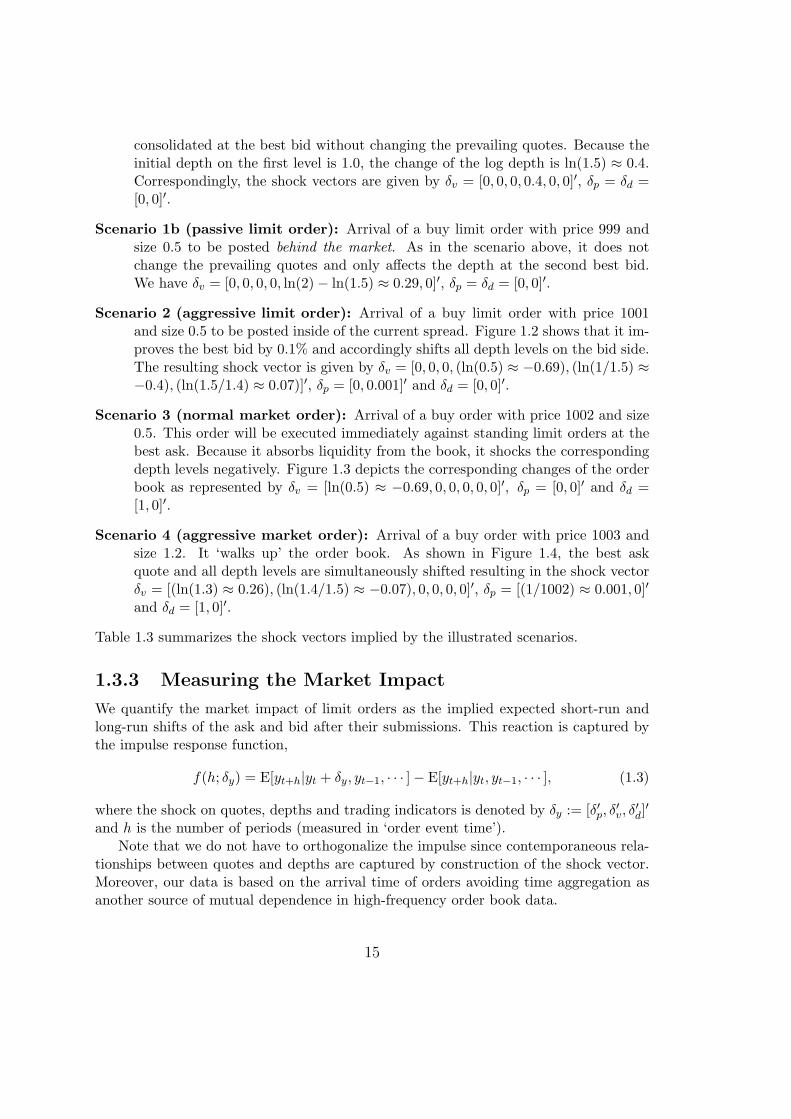
Figure 1.8: Changes of ask and bid quotes induced by buy/sell limit orders placed atthe market (level one) with a size equal to the half of the depth on the first level. Themarked number on the vertical axes indicates the magnitude of the permanent impact.The blue dotted lines indicate the corresponding 95%-confidence intervals. Trading ofFortis at Euronext, Amsterdam in August 2008. LO: limit order.
orders with a size equal to half of the depth at the best quotes.11 The impulse responsefunction starts at zero since such a limit order does not directly change the ask and bid.As expected, both ask and bid tend to significantly increase (decrease) after the arrivalof a buy (sell) limit order. Induced by the cointegration setting, quotes converge to a(new) permanent level at which the information content of the incoming limit order iscompletely incorporated. The confidence intervals reflect that the shift is statisticallyhighly significant.
We observe that quotes adjust relatively quickly reaching the new level after approx-imately 20 lags. Recall that time is measured in terms of limit order book activities.Hence, the adjustment speed measured in physical time ultimately depends on the un-derlying frequency of order activities and differs across the market. However, the factthat the speed of stock-specific quote adjustments (in terms of a ‘limit order clock’) iswidely stable across the market, indicates that such a business time scale is appropriatefor market-wide comparisons across stocks.
An interesting fact is that after the arrival of a buy limit order, the bid tends toincrease more quickly than the ask. A reverse effect is observed after the arrival ofa sell limit order. This asymmetry introduces a one-sided and temporary decrease ofthe bid-ask spread. We explain this phenomenon by the fact that traders observing
11In all figures illustrating impulse responses, the legend ‘A → B’ is interpreted to reflect ‘theimpact on B induced by A’.
25

an incoming limit order on the same side of the market tend to compete for providedliquidity by undercutting quotes. Moreover, the higher depth at the bid generates a(delayed) liquidity demand on the ask side shifting upward the ask as well. We thusrefer this phenomenon to be a liquidity-motivated effect.
Our findings can be interpreted in terms of pure market mechanisms. The marketequilibrium is perturbed by a limit order in two ways. On one hand, the limit orderindicates an investor’s willingness to buy or sell and thus increases the supply or de-mand of the underlying asset. The market price changes to incorporate this temporaryimbalance of supply and demand. One the other hand, an incoming limit order increasesthe supply of liquidity in the market. A narrowing of the spread reduces transactioncosts and causes a re-balancing of supply and demand of liquidity. See, e.g., the simu-lation study by Yamamoto (2011) on the effects of the state of the limit order book oninvestors’ strategies.
The significant permanent impact induced by an incoming limit order indicates thatit contributes to price discovery. Thus, market participants perceive that limit orderscarry private information which is in contrast to the common assumption in theoreticalliterature that informed traders only take liquidity but do not provide it. On the otherhand, it is supported by the experiment by Bloomfield, O’Hara, and Saar (2005) showingthat informed traders use order strategies involving both market orders and limit ordersto optimally capitalize their informational advantage and in line with Mike and Farmer(2008) and Chiarella, Iori, and Perello (2009) suggesting that there is a link between theproperties of order flow and those of prices.
Given the setting of the book we observe that a limit order increasing first leveldepth by 50% shifts quotes by 0.5 to 0.6 basis points. Though this effect is generallyrather small, it is economically significant if the tick size is small. Moreover, note thatthe magnitude of the market impact is log-linear in the order size. In practice, a biglimit order posted on a thin order book might affect the market much more stronglythan in our scenarios.
In order to explore the role of the order’s position in the book, Figure 1.9 depictsthe bid prices’ reactions induced by buy limit orders placed at the market (level one)and behind the market (level two and three). We observe a negative correlation betweenthe magnitude of quote reactions and the orders’ distance from the spread. The at-the-market limit order induces significantly faster market reactions than the behind-the-market limit order. Nonetheless, the long-term impact of level one and level two limitorders is only approximately 20% smaller. Hence, it turns out that behind-the-marketorders can significantly shift the market though the quote adjustment is slower.12 Thisresult holds for level two orders and (to a weaker extent) for level three orders. However,for orders posted deeper in the book virtually no market impacts can be identified.
Eom, Lee, and Park (2009) find evidence that traders could have made extra profitsusing microstructure-based manipulations on the Korean Exchange (KRX) during aperiod between 2001 and 2002. In this period, KRX disclosed the total quantity on each
12In order to improve the graphical illustrations, we refrain from showing the correspondingconfidence intervals. They are quite similar to those shown in Figure 1.8.
26

0 5 10 15 20 25 30 35 40 45 50−0.1
0
0.1
0.2
0.3
0.4
0.5
0.6
0.533
0.41
0.145
Event time
Quo
te C
hang
e (B
asis
Poi
nt)
L1 buy LO → BidL2 buy LO → BidL3 buy LO → bidPermanent Impact
Figure 1.9: Changes of bid quotes induced by buy limit orders placed at the market(level one) and behind the market (level two and three). The order size equals to half ofthat at the best bid. The initial order book equals the corresponding monthly averageshown in Table 1.1. The marked number on the vertical axes indicates the magnitudeof the permanent impact. Trading of Fortis at Euronext, Amsterdam in August, 2008.L1: level one. L2: level two. L3: level three. LO: limit order.
27

0 5 10 15 20 250
0.5
1
1.5
2
2.5
3
3.5
4
4.5
5
1.82
Event time
Quo
te C
hang
e (B
asis
Poi
nt)
Buy LO → AskBuy LO → BidPermanent Impact
0 5 10 15 20 25 30 35 40 45 501.5
2
2.5
3
3.5
4
4.5
5
5.5
6
1.82
4.84
5.37
Event time
Quo
te C
hang
e (B
asis
Poi
nt)
Small buy LO → Bid Mid buy LO → BidBig buy LO → BidPermanent Impact
Figure 1.10: Left: Changes of quotes induced by buy limit orders placed inside of thespread with a size equal to the depth at the bid. Right: Changes of bid induced bybuy limit orders placed inside of the spread with different sizes. The initial order bookequals to the corresponding monthly average shown in Table 1.1. Small size: depth atthe bid. Mid size: 7 times of the depth at the bid. Big size: 15 times of the depth atthe bid. Trading of Fortis at Euronext, Amsterdam in August, 2008. LO: limit order.
side of LOB without fully disclosing the prices at which these orders have been placed.The manipulation strategy resulted in placing huge numbers of behind-the-market limitorders on the opposite side of the market inducing price moves in the favorite directionwithout having these orders executed. Our finding shows that this kind of manipulationis indeed possible. However, whether it is economically profitable in Euronext ultimatelydepends on (relative) order sizes. In order to move quotes in her favorite direction, thetrader has to submit rather big limit orders close to the market. Then, she faces the riskthat these orders may be picked up.
1.5.2 Limit Orders Placed Inside Of the Spread
Limit orders placed inside of the bid-ask spread perturb the LOB dynamics in a morecomplex way. Apart from providing liquidity to the order book, they directly improvethe ask or bid. This quote adjustment induces a reduction of the spread, establishes anew best quote level and correspondingly shifts all depth levels on the corresponding sideof the book upward (or downward, respectively). The system seeks the new equilibriumon a path recovering from the immediate quote change and simultaneously re-balancingliquidity. Given our setting, we assume that a buy limit order inside of the spread inducesa 5 basis points increase of the bid. However, as shown in the left plot of Figure 1.10,the long-run price impact is just 1.8 basis points. The immediate quote movement isreverted back by approximately 65%. This is induced either by sell trades picking up
28

0 5 10 15 20 25 30 35 40 45 50−3
−2
−1
0
1
2
3
4
2.55
−2.2
Event time
Quo
te C
hang
e (B
asis
Poi
nt)
Buy MO → AskBuy MO → BidSell MO → AskSell MO → Bid95% confindence intervalPermanent Impact
Figure 1.11: Changes of quotes induced by buy/sell market orders (buyer-/seller-initiated trades) with a size equal to half of the depth on their corresponding first levels.The marked number on the vertical axes indicates the magnitude of the permanentimpact. Trading of Fortis at Euronext, Amsterdam in August, 2008. MO: Market order.
the posted volume or by cancellations on the bid side. Similarly, liquidity demand onthe ask side shifts the ask upward by 1.8 basis points. Hence, overall we observe anasymmetric re-balancing of quotes and a corresponding re-widening of the spread.
The right plot of Figure 1.10 compares the effects of buy limit orders of differentsizes but with same limit price posted inside of the bid-ask spread and thus improvingbid quotes again by 5 basis points. We observe quite different impulse response patternsin dependence of the order size. In case of a comparably small order, the posted volumeis quickly picked up, shifting back the bid quote. In contrast, large volumes overbiddingthe prevailing quote cause a long-term upward movement of the bid. Relative to theinitial shift of the bid we observe a further approximately 20% price increase. Hence,extraordinary large orders are not likely to be picked up and induce a rather strongbuy pressure moving the market upwards. For smaller (though still comparably large)orders, adverse selection and signaling effects seem to counterbalance each other. Asa consequence, the bid quote is hardly changed and the long run effect is close to theimmediate price improvement.
1.5.3 Market Impact of Trades
Figure 1.11 shows the market impacts induced by buy and sell market orders. Weassume that the trade sizes correspond to 50% of the prevailing depth. Consequently,these market orders do not ‘walk through’ the limit order book and thus ask and bid
29
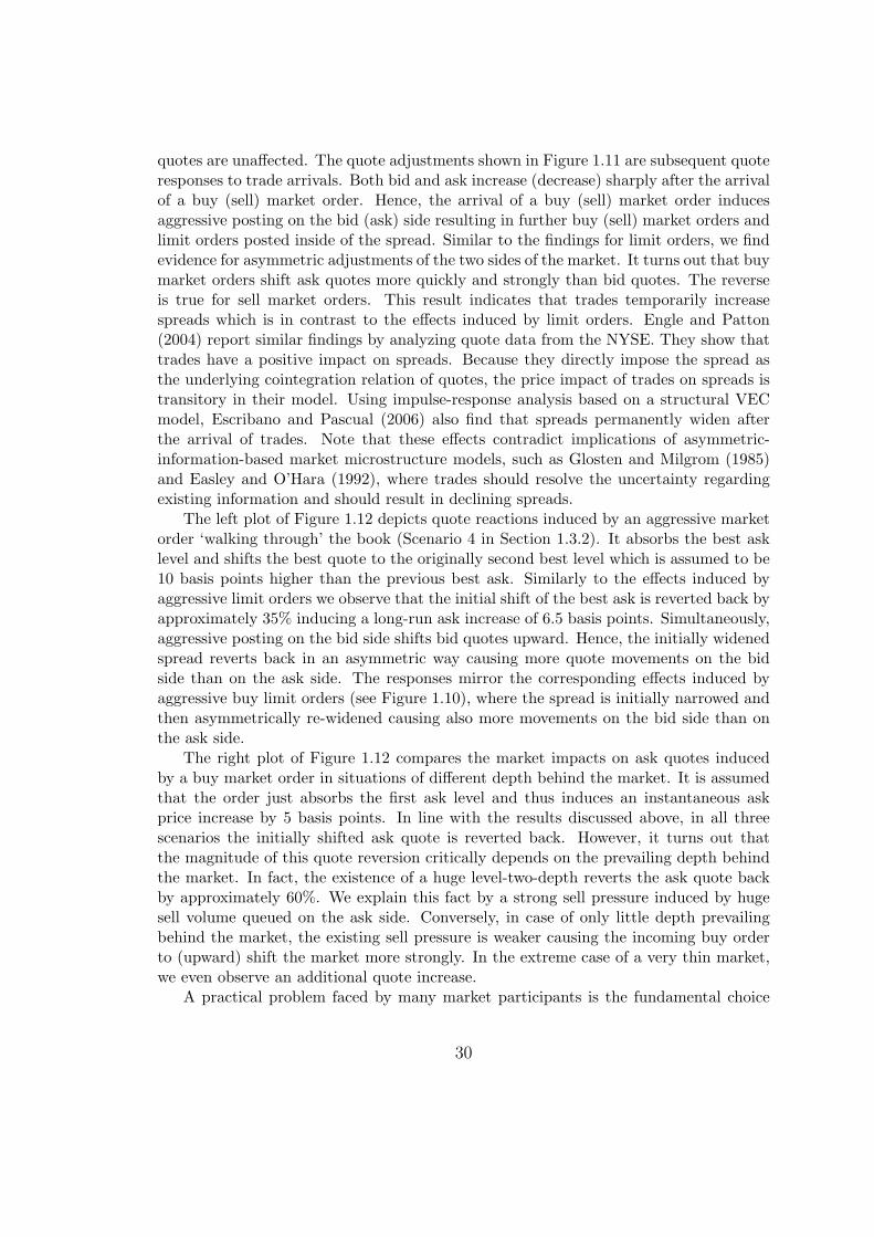
quotes are unaffected. The quote adjustments shown in Figure 1.11 are subsequent quoteresponses to trade arrivals. Both bid and ask increase (decrease) sharply after the arrivalof a buy (sell) market order. Hence, the arrival of a buy (sell) market order inducesaggressive posting on the bid (ask) side resulting in further buy (sell) market orders andlimit orders posted inside of the spread. Similar to the findings for limit orders, we findevidence for asymmetric adjustments of the two sides of the market. It turns out that buymarket orders shift ask quotes more quickly and strongly than bid quotes. The reverseis true for sell market orders. This result indicates that trades temporarily increasespreads which is in contrast to the effects induced by limit orders. Engle and Patton(2004) report similar findings by analyzing quote data from the NYSE. They show thattrades have a positive impact on spreads. Because they directly impose the spread asthe underlying cointegration relation of quotes, the price impact of trades on spreads istransitory in their model. Using impulse-response analysis based on a structural VECmodel, Escribano and Pascual (2006) also find that spreads permanently widen afterthe arrival of trades. Note that these effects contradict implications of asymmetric-information-based market microstructure models, such as Glosten and Milgrom (1985)and Easley and O’Hara (1992), where trades should resolve the uncertainty regardingexisting information and should result in declining spreads.
The left plot of Figure 1.12 depicts quote reactions induced by an aggressive marketorder ‘walking through’ the book (Scenario 4 in Section 1.3.2). It absorbs the best asklevel and shifts the best quote to the originally second best level which is assumed to be10 basis points higher than the previous best ask. Similarly to the effects induced byaggressive limit orders we observe that the initial shift of the best ask is reverted back byapproximately 35% inducing a long-run ask increase of 6.5 basis points. Simultaneously,aggressive posting on the bid side shifts bid quotes upward. Hence, the initially widenedspread reverts back in an asymmetric way causing more quote movements on the bidside than on the ask side. The responses mirror the corresponding effects induced byaggressive buy limit orders (see Figure 1.10), where the spread is initially narrowed andthen asymmetrically re-widened causing also more movements on the bid side than onthe ask side.
The right plot of Figure 1.12 compares the market impacts on ask quotes inducedby a buy market order in situations of different depth behind the market. It is assumedthat the order just absorbs the first ask level and thus induces an instantaneous askprice increase by 5 basis points. In line with the results discussed above, in all threescenarios the initially shifted ask quote is reverted back. However, it turns out thatthe magnitude of this quote reversion critically depends on the prevailing depth behindthe market. In fact, the existence of a huge level-two-depth reverts the ask quote backby approximately 60%. We explain this fact by a strong sell pressure induced by hugesell volume queued on the ask side. Conversely, in case of only little depth prevailingbehind the market, the existing sell pressure is weaker causing the incoming buy orderto (upward) shift the market more strongly. In the extreme case of a very thin market,we even observe an additional quote increase.
A practical problem faced by many market participants is the fundamental choice
30

0 5 10 15 20 25 30 350
1
2
3
4
5
6
7
8
9
10
6.51
Event time
Quo
te C
hang
e (B
asis
Poi
nt)
Buy MO → AskBuy MO → BidPermanent Impact
0 5 10 15 20 25 30 352
3
4
5
6
7
8
7.4
4.23
2.01
Event time
Quo
te C
hang
e (B
asis
Poi
nt)
Buy MO → Ask (less liquidity behind market)Buy MO → Ask (mid liquidity behind market)Buy MO → Ask (huge liquidity behind market)Permanent Impact
Figure 1.12: Left: Changes of bid and ask quotes induced by an aggressive buy marketorder with a size exceeding the depth at the best ask by 20%. The second best ask isassumed to be 5 basis points higher than the ask, where the depths behind the marketare 1.5 times of the depth at the market. Right: Changes of ask quotes induced byan aggressive buy market order with a size equal to the depth at the ask when thereis different depth at the second best ask. Case 1: the depth at the second best ask is10% of that at the ask; Case 2: the depth at the second best ask equals to that at theask; Case 3: the depth at the second best ask is 500% of that at the ask. The markednumber on the vertical axes indicate the magnitude of the permanent impact. Tradingof Fortis at Euronext, Amsterdam in August, 2008. MO: Market order.
31

0 5 10 15 20 25 30 350
0.5
1
1.5
2
2.5
3
2.55
0.533
Event time
Quo
te C
hang
e (B
asis
Poi
nt)
Buy MO → Ask Buy MO → BidBuy LO → AskBuy LO → BidPermanent Impact
Figure 1.13: Changes of ask and bid quotes induced by a buy market order and a buylimit order of similar size placed at the market. The order size is half of the depth at thebest bid. The depths at the best bid and the best ask in the order book are assumed tobe equal. Trading of Fortis at Euronext, Amsterdam in August, 2008. LO: limit order;MO: market order.
between posting a market order and a limit order. A direct comparison of the marketimpacts induced by these two types of orders is shown in Figure 1.13. In both cases, theposted order does not directly change quotes. We observe that the resulting long-runeffect of trades is significantly greater than that of an equal-size limit order. Actually,the price shift induced by a market order is approximately four times larger than thatof a comparable limit order. This finding is consistent with the theoretical predictionby Rosu (2010). Moreover, market orders also cause quicker market reactions. Finally,inferred from the ‘gap’ between ask and bid curves, market orders change the spreadmore dramatically than limit orders. Hence, the willingness to cross the bid-ask spreadis a stronger signal for private information than that induced by a comparable limitorder.
Note that the comparison holds for ‘normal’ order types placed on the best quote, butnot necessarily for more aggressive orders. As discussed above, the long-term effects ofaggressive limit orders and market orders critically depend on their (relative) size and thecurrent state of the book. Therefore, an ultimate comparison of market impacts inducedby both types of orders under comparable conditions is rather difficult. Nevertheless, ourresults show that limit orders do have a significant long-term effect and can significantly‘scare’ the market.
32
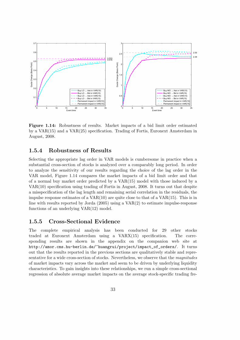
0 5 10 15 20 25 30 350
0.1
0.2
0.3
0.4
0.5
0.6
0.7
0.5150.533
Event time
Quo
te C
hang
e (B
asis
Poi
nt)
Buy LO → Ask in VAR(10)Buy LO → Bid in VAR(10)Buy LO → Ask in VAR(15)Buy LO → Bid in VAR(15)Permanent impact in VAR(10)Permanent impact in VAR(15)
0 5 10 15 20 25 30 350
0.5
1
1.5
2
2.5
3
2.35
2.55
Event time
Quo
te C
hang
e (B
asis
Poi
nt)
Buy MO → Ask in VAR(10)Buy MO → Bid in VAR(10)Buy MO → Ask in VAR(15)Buy MO → Bid in VAR(15)Permanent impact in VAR(10)Permanent impact in VAR(15)
Figure 1.14: Robustness of results. Market impacts of a bid limit order estimatedby a VAR(15) and a VAR(25) specification. Trading of Fortis, Euronext Amsterdam inAugust, 2008.
1.5.4 Robustness of Results
Selecting the appropriate lag order in VAR models is cumbersome in practice when asubstantial cross-section of stocks is analyzed over a comparably long period. In orderto analyze the sensitivity of our results regarding the choice of the lag order in theVAR model, Figure 1.14 compares the market impacts of a bid limit order and thatof a normal buy market order predicted by a VAR(15) model with those induced by aVAR(10) specification using trading of Fortis in August, 2008. It turns out that despitea misspecification of the lag length and remaining serial correlation in the residuals, theimpulse response estimates of a VAR(10) are quite close to that of a VAR(15). This is inline with results reported by Jorda (2005) using a VAR(2) to estimate impulse-responsefunctions of an underlying VAR(12) model.
1.5.5 Cross-Sectional Evidence
The complete empirical analysis has been conducted for 29 other stockstraded at Euronext Amsterdam using a VARX(15) specification. The corre-sponding results are shown in the appendix on the companion web site athttp://amor.cms.hu-berlin.de/~huangrui/project/impact_of_orders/. It turnsout that the results reported in the previous sections are qualitatively stable and repre-sentative for a wide cross-section of stocks. Nevertheless, we observe that the magnitudesof market impacts vary across the market and seem to be driven by underlying liquiditycharacteristics. To gain insights into these relationships, we run a simple cross-sectionalregression of absolute average market impacts on the average stock-specific trading fre-
33
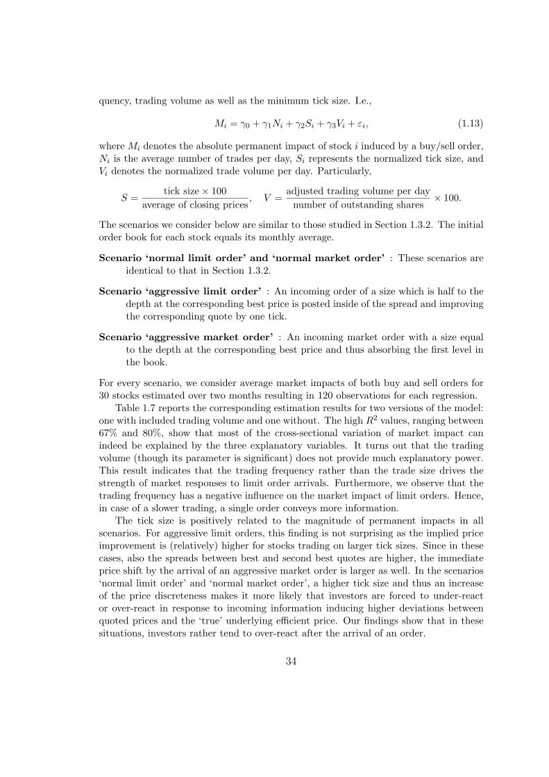
quency, trading volume as well as the minimum tick size. I.e.,
Mi = γ0 + γ1Ni + γ2Si + γ3Vi + εi, (1.13)
where Mi denotes the absolute permanent impact of stock i induced by a buy/sell order,Ni is the average number of trades per day, Si represents the normalized tick size, andVi denotes the normalized trade volume per day. Particularly,
S =tick size× 100
average of closing prices, V =
adjusted trading volume per day
number of outstanding shares× 100.
The scenarios we consider below are similar to those studied in Section 1.3.2. The initialorder book for each stock equals its monthly average.
Scenario ‘normal limit order’ and ‘normal market order’ : These scenarios areidentical to that in Section 1.3.2.
Scenario ‘aggressive limit order’ : An incoming order of a size which is half to thedepth at the corresponding best price is posted inside of the spread and improvingthe corresponding quote by one tick.
Scenario ‘aggressive market order’ : An incoming market order with a size equalto the depth at the corresponding best price and thus absorbing the first level inthe book.
For every scenario, we consider average market impacts of both buy and sell orders for30 stocks estimated over two months resulting in 120 observations for each regression.
Table 1.7 reports the corresponding estimation results for two versions of the model:one with included trading volume and one without. The high R2 values, ranging between67% and 80%, show that most of the cross-sectional variation of market impact canindeed be explained by the three explanatory variables. It turns out that the tradingvolume (though its parameter is significant) does not provide much explanatory power.This result indicates that the trading frequency rather than the trade size drives thestrength of market responses to limit order arrivals. Furthermore, we observe that thetrading frequency has a negative influence on the market impact of limit orders. Hence,in case of a slower trading, a single order conveys more information.
The tick size is positively related to the magnitude of permanent impacts in allscenarios. For aggressive limit orders, this finding is not surprising as the implied priceimprovement is (relatively) higher for stocks trading on larger tick sizes. Since in thesecases, also the spreads between best and second best quotes are higher, the immediateprice shift by the arrival of an aggressive market order is larger as well. In the scenarios‘normal limit order’ and ‘normal market order’, a higher tick size and thus an increaseof the price discreteness makes it more likely that investors are forced to under-reactor over-react in response to incoming information inducing higher deviations betweenquoted prices and the ‘true’ underlying efficient price. Our findings show that in thesesituations, investors rather tend to over-react after the arrival of an order.
34

Table 1.7Cross-sectional analysis of market impacts over the market.We consider market impacts of both buy and sell orders for 30 stocks estimated over
August and September, 2008. The regression is Mi = γ0 + γ1Ni + γ2Si + γ3Vi + εi,where Mi denotes the absolute permanent impact of stock i induced by a buy/sell limitorder, Ni is the average number of trades per day, Si represents the normalized tick size,and Vi denotes the normalized trade volume per day. The numbers in brackets denoteheteroskedasticity robust t−statistics according to White (1980).
Scenario γ0 γ1 γ2 γ3 R2
‘normal limit order’ 0.0033 −0.0013 0.0418 – 0.69(19.02) (−7.30) (33.72)0.0027 −0.0015 0.040 0.0011 0.73(13.77) (−11.35) (34.85) (6.5)
‘aggressive 0.005 −0.0017 0.096 – 0.79limit order’ (13.12) (−5.93) (23.04)
0.004 −0.002 0.095 0.001 0.80(11.98) (−7.92) (22.80) (8.34)
‘normal market order’ 0.037 −0.016 0.17 −− 0.57(21.94) (−9.26) (6.33)0.030 −0.018 0.151 0.013 0.67(14.59) (−16.74) (5.56) (7.49)
‘aggressive 0.049 −0.020 0.474 −− 0.68market order’ (19.89) (−8.24) (14.46)
0.039 −0.023 0.449 0.018 0.75(13.03) (−15.06) (14.07) (7.22)
35

1.6 Conclusion
In this chapter, we quantify the market impact of incoming limit orders in a limit orderbook market. Best bid and ask quotes as well as three levels of depth on both sides ofthe market are modeled based on a cointegrated VAR system. Incoming limit orders arerepresented in terms of shocks to the system. Limit order characteristics as well as thecorresponding state of the book are captured by the specific design of the shock vector.This allows us to distinguish between limit orders of different aggressiveness (reflectedby their distance to the market) and different sizes as well as between different statesof the book. The market impacts on ask and bid prices are quantified by the estimatedimpulse response function using appropriate statistical inference.
Employing this framework we analyze the limit order book processes of 30 stockstraded on Euronext Amsterdam over two months in 2008. The model is estimated usingthe highest possible frequency accounting for all order book changes during continuoustrading. Parameter estimates and diagnostics indicate that the proposed model capturesthe high-frequency order book dynamics quite well.
Based on the empirical analysis we can summarize the following findings: First, wefind clear evidence for cointegration relations between ask and bid quotes and corre-sponding depths. While some cointegration relations are similar to the bid-ask spread,others show that depth has a distinct effect on quote dynamics and on the connectionbetween ask and bid quotes. Second, limit orders do have significant long-term effectson quotes. This is even true for limit orders placed behind the market though these ef-fects decline with the limit order’s distance to the market. While incoming limit orderstemporarily decrease the spread, market orders induce a temporary widening. Third,the speed of spread convergence as well as the direction of price movements after thearrival of aggressive limit orders undercutting (or overbidding, respectively) best ask andbid prices strongly depends on the incoming limit order’s size. While small orders seemto face adverse selection risks and are likely to be picked up quickly, for larger ordersinformation signaling effects seem to dominate pushing the market in the opposite di-rection. Fourth, the decrease (increase) of spreads after the arrival of an aggressive limit(market) order is reverted back asymmetrically inducing more quote movements on theside where the order has been placed. Fifth, the long-run market impact of aggressivemarket orders walking through the book rises with the queued depth behind the market.Sixth, the effects are qualitatively remarkably stable over the cross-section of the market.Variations in the magnitudes of market impacts are well explained by the underlyingstock-specific trading frequency and minimum tick size.
Our empirical results also show that the proposed framework is useful and appro-priate to capture order book dynamics on high frequencies. By modeling quotes andseveral levels of depth, the model implicitly captures also the multivariate dynamicsof mid-quotes, returns, spreads, spread changes as well as depth imbalances. In thissense, the suggested high-frequency cointegrated VAR model can serve as a workhorsefor various applications in this area.
36
Chapter 2
Limit Order Properties andOptimal Order Sizes
This chapter is based on Hautsch and Huang (2012a).
2.1 Introduction
Electronic limit order book (LOB) systems are the dominant trading form of most fi-nancial markets worldwide, including leading exchanges like NASDAQ, NYSE, BATSand Euronext, various Alternative Trading Systems (ATSs) and Electronic Communica-tion Networks (ECNs). The recent decade witnesses substantial technological progressin trading systems as well as trade recording and an increasing importance of intra-day trading. Transparency, low latency, high liquidity and low trading costs attractan increasing number of intraday traders, long-horizon traders as well as institutionalinvestors. Though electronic limit order book trading already exists for many years, fur-ther developments in trading systems and structures are ongoing and are faster than everbefore. The successive automatization of order management and execution by computeralgorithms, the growing importance of smart order routing as well as changes of marketstructures and trading forms challenge empirical and theoretical market microstructureresearch.
The objective of this chapter is to provide new empirical evidence on order activitiesand market dynamics at NASDAQ – the largest electronic market for equities in the U.S.By employing TotalView-ITCH data containing information directly stemming from theNASDAQ data feed, our study sheds some light on recent order arrival rates, executionrates, cancellation rates and the price impact of incoming quotes. Particularly the marketimpact of a limit order is a key parameter for trading decisions and play a crucial rolefor (algorithmic) trading strategies. Also theoretical studies, such as, e.g., Harris (1997),Parlour and Seppi (2008), Boulatov and George (2008) or Rosu (2010), predict that therevelation of a trading intention by limit order placements can indeed adversely affectasset prices. Despite of its importance, empirical evidence on the influence of incoming
37

limit orders is still limited. Only very recently, Hautsch and Huang (2012b), Eisler,Bouchaud, and Kockelkoren (2011) and Cont, Kukanov, and Stoikov (2011) analyze theprice impact of limit orders and find significant effects. In this study, we employ Hautschand Huang’s (2012b) framework, which extends the approach by Engle and Patton (2004)and provides deeper insights into the market impact of limit orders in recent NASDAQtrading. Of particular interest is whether the magnitudes of price impacts identified inother markets are also found in the extremely liquid NASDAQ market and which limitorder sizes can be ultimately posted without significantly moving the market.
TotalView-ITCH data contains all order messages and thus allows us to reconstructthe NASDAQ limit order book in a very precise way, particularly accounting for allhigh-frequency limit order activities including also so-called fleeting orders. The latterare present for only few seconds and have the purpose of testing for hidden ordersplaced in the bid-ask spread. A detailed analysis of the NASDAQ order flow in October2010 provides the following major results: First, the number of limit order submissionsis twenty to forty higher than the number of trades. Secondly, limit order sizes aretypically small and clustered at round lot sizes of hundred shares. Third, more than95% of all limit orders are cancelled without getting executed with most of them beingcancelled nearly instantaneously (less than one second) after their submission reflectingthe proliferation of algorithmic trading at NASDAQ. Fourth, volume-weighted executiontimes are significantly greater than average execution times indicating that large ordersface more execution risk than small ones.
The market impact of limit orders is quantified by modeling ask and bid quotes andseveral levels of depth in terms of a cointegrated vector-autoregressive (VAR) systemwhich is updated in event time. Short-run and long-run quote reactions are quanti-fied by impulse-response functions. As proposed by Hautsch and Huang (2012b), thisframework allows us to estimate the impact of specific limit order activities includinglimit order submissions, cancellations and executions (corresponding to trades) whichare represented as shocks to the system. Our empirical results show that the short-runand long-run quote reaction patterns after the arrival of a limit order are indeed quitesimilar to those, for example found for Euronext Amsterdam (see Hautsch and Huang,2012b). Buy (sell) limit orders cause permanent quote increases (decreases) and a tem-porary decline of the spread. Moreover, we find that the permanent impact of a limitorder posted at the best quote is in most cases approximately 25% of that of a tradeof similar size. However, this magnitude can be much smaller when hidden orders areplaced inside of the spread. As on other liquid markets, only aggressive limit ordersposted on the first or second order level induce significant price impacts whereas ordersposted with greater distance to the market have virtually no effect.
Finally, using the estimates of market impacts, we suggest a way to compute theoptimal size of a limit order given its expected price impact. The implied order size iscalculated by inverting the closed form of the permanent impact yielding a function ofthe current limit order book and the given market impact control level. This providesuseful information to control risks in trading strategies.
The remainder of this chapter is organized in the following way. Section 2.2 briefly
38

introduces the market environment and the data. Section 2.3 provides an explorativeanalysis of the order flow. The econometric framework is reviewed in Section 2.4. Sec-tion 2.5 gives empirical evidence of short-run and long-run quote reactions on orderactivities. In Section 2.6, we propose a method to compute the optimal order size sub-ject to its position in the book and the expected market impact. Finally, Section 2.7concludes.
2.2 Market Environment and Data
The NASDAQ stock market is the largest electronic stock market (in terms of tradingvolume) in the world. In 2006, its traditional market center, Brut and INET electroniccommunication networks (ECNs) are integrated into a single system. This system offersa single execution algorithm based on price and time order precedence for both marketmakers and participants of ECNs. During the continuous trading period between 9:30and 16:00 EST, limit orders are submitted to a centralized computer system where theyare matched to prevailing limit or hidden orders on the opposite side. If there is no matchor the standing volume in the system is insufficient to fully execute the incoming order,the remaining order volume is placed in the order book. NASDAQ supports various ordertypes like pure market orders (immediate order execution without a price limit), stoporders (automatic issuing of limit orders or market orders when a given price is reached),immediate-or-cancel (IOC) orders, reserve orders and non-display orders, among others.
In this study, we use TotalView-ITCH data containing rich information on orderactivities. The database includes limit order submissions, cancellations, executions andhidden order executions for every trading day since 7:00am EST when the system startsaccepting incoming limit orders. The system is initialized by an empty order book whereall overnight limit orders are resubmitted automatically at the beginning of each day.Therefore, we can exactly reconstruct the order book at any time by aggregating theexisting visible limit orders according to their limit prices. Furthermore, NASDAQ To-talView, surpassing NASDAQ Level 2, is the standard NASDAQ data feed for displayingthe full order book depth for market participants. Hence, the reconstructed order bookexactly represents historical real-time-disseminated order book states. Trades are iden-tified via the records of limit orders and hidden order executions. Since the tradingdirection of limit orders and hidden orders is recorded, we can exactly identify whethera trade is buyer-initiated or seller-initiated. Finally, TotalView-ITCH data records aunique identification of any limit order which allows to track the order and to compute,for instance, its life-time.1
Note that a market order, especially when its order size is comparably large, islikely to be filled by several pending limit orders. This results in multiple limit orderexecutions corresponding to a sequence of same-type (sub-)trades within a short time
1The limit order book reconstruction and limit order tracking is performed by thesoftware ”LOBSTER” (see Huang and Polak, 2011), which can be freely accessed athttp://lobster.wiwi.hu-berlin.de.
39
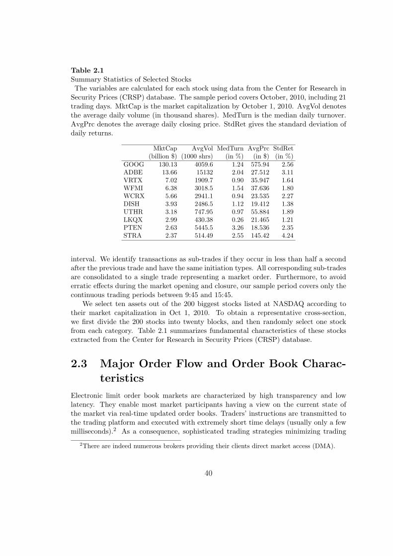
Table 2.1Summary Statistics of Selected StocksThe variables are calculated for each stock using data from the Center for Research in
Security Prices (CRSP) database. The sample period covers October, 2010, including 21trading days. MktCap is the market capitalization by October 1, 2010. AvgVol denotesthe average daily volume (in thousand shares). MedTurn is the median daily turnover.AvgPrc denotes the average daily closing price. StdRet gives the standard deviation ofdaily returns.
MktCap AvgVol MedTurn AvgPrc StdRet(billion $) (1000 shrs) (in %) (in $) (in %)
GOOG 130.13 4059.6 1.24 575.94 2.56ADBE 13.66 15132 2.04 27.512 3.11VRTX 7.02 1909.7 0.90 35.947 1.64WFMI 6.38 3018.5 1.54 37.636 1.80WCRX 5.66 2941.1 0.94 23.535 2.27DISH 3.93 2486.5 1.12 19.412 1.38UTHR 3.18 747.95 0.97 55.884 1.89LKQX 2.99 430.38 0.26 21.465 1.21PTEN 2.63 5445.5 3.26 18.536 2.35STRA 2.37 514.49 2.55 145.42 4.24
interval. We identify transactions as sub-trades if they occur in less than half a secondafter the previous trade and have the same initiation types. All corresponding sub-tradesare consolidated to a single trade representing a market order. Furthermore, to avoiderratic effects during the market opening and closure, our sample period covers only thecontinuous trading periods between 9:45 and 15:45.
We select ten assets out of the 200 biggest stocks listed at NASDAQ according totheir market capitalization in Oct 1, 2010. To obtain a representative cross-section,we first divide the 200 stocks into twenty blocks, and then randomly select one stockfrom each category. Table 2.1 summarizes fundamental characteristics of these stocksextracted from the Center for Research in Security Prices (CRSP) database.
2.3 Major Order Flow and Order Book Charac-
teristics
Electronic limit order book markets are characterized by high transparency and lowlatency. They enable most market participants having a view on the current state ofthe market via real-time updated order books. Traders’ instructions are transmitted tothe trading platform and executed with extremely short time delays (usually only a fewmilliseconds).2 As a consequence, sophisticated trading strategies minimizing trading
2There are indeed numerous brokers providing their clients direct market access (DMA).
40

0 1 2 3 4 50
1
2
3
4
5
6
7
8x 10⁵
log10(order sizes)0 0.5 1 1.5 2 2.5 3 3.5 4
0
1
2
3
4
5
6
7x 10⁴
log10(executed sizes)
−3 −2 −1 0 1 2 3 4 50
2
4
6
8
10
12
14
16
18x 104
log10(cancellation time)−4 −2 0 2 4 60
2000
4000
6000
8000
10000
12000
14000
log10(execution time)
Figure 2.1: Histogram of order sizes, execution sizes, cancellation times and executiontimes of limit orders. The red line denotes kernel density estimates. Zero cancellationtimes and execution times are discarded. Trading of WCRX on NASDAQ in October,2010.
costs and exploiting high-frequency price movements are performed using computer al-gorithms. Triggered by technological advances, systematic trading is highly sophisticatednowadays. For instance, in order to make profit from high-frequency price fluctuationsand liquidity rebates, many high-frequency trading algorithms post a huge number oflimit orders which are again canceled almost immediately if not getting executed. As aconsequence, enormous limit order activities on extremely high frequencies are observed.
Table 2.2 summarizes the limit order activities of selected stocks and Figure 2.1 shows
41
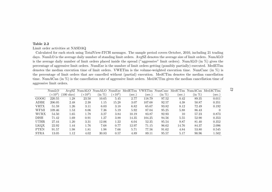
Table 2.2Limit order activities at NASDAQCalculated for each stock using TotalView-ITCH messages. The sample period covers October, 2010, including 21 trading
days. NumLO is the average daily number of standing limit orders. AvgSZ denotes the average size of limit orders. NumALOis the average daily number of limit orders placed inside the spread (”aggressive” limit orders). NumALO (in %) gives thepercentage of aggressive limit orders. NumExe is the number of limit orders getting (possibly partially) executed. MedETimdenotes the median execution time of limit orders. VWETim is the volume-weighted execution time. NumCanc (in %) isthe percentage of limit orders that are cancelled without (partial) execution. MedCTim denotes the median cancellationtime. NumACan (in %) is the cancellation rate of aggressive limit orders. MedACTim gives the median cancellation time ofaggressive limit orders.
NumLO AvgSZ NumALO NumALO NumExe MedETim VWETim NumCanc MedCTim NumACan MedACTim(×103) (100 shrs) (×103) (in %) (×103) (sec.) (sec.) (in %) (sec.) (in %) (sec.)
GOOG 220.55 1.28 23.50 10.65 5.45 2.77 118.79 97.52 0.42 89.35 0.011ADBE 206.05 2.48 2.38 1.15 15.28 3.07 107.68 92.57 4.38 50.87 0.351VRTX 51.59 1.26 3.11 6.03 3.18 6.82 65.67 93.82 8.12 72.49 0.192WFMI 109.46 1.53 8.06 7.36 5.19 5.92 87.04 95.25 5.88 86.43 0WCRX 54.50 1.65 1.78 3.27 3.84 10.19 83.87 92.93 10 57.23 0.873DISH 71.42 1.69 0.91 1.27 3.88 14.35 104.25 94.56 5.55 52.90 0.353UTHR 27.44 1.20 3.31 12.06 1.22 6.04 52.35 95.54 9.87 81.40 0.352LKQX 22.92 1.44 1.76 7.68 0.77 12.97 71.15 96.62 14.76 84.37 2.096PTEN 91.57 1.98 1.81 1.98 7.66 5.71 77.56 91.62 4.84 53.80 0.545STRA 13.05 1.12 4.02 30.83 0.57 4.89 89.11 95.57 5.17 90.96 1.502
42
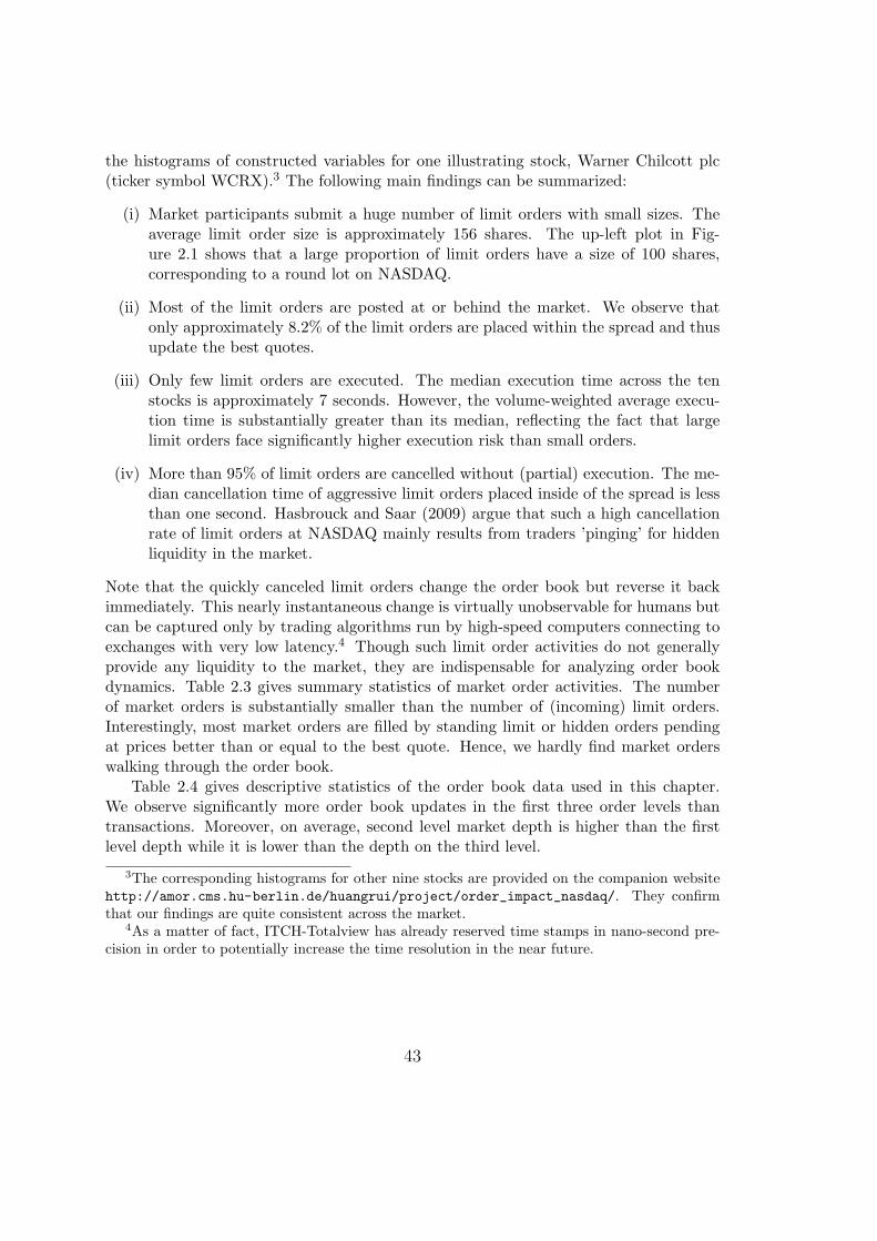
the histograms of constructed variables for one illustrating stock, Warner Chilcott plc(ticker symbol WCRX).3 The following main findings can be summarized:
(i) Market participants submit a huge number of limit orders with small sizes. Theaverage limit order size is approximately 156 shares. The up-left plot in Fig-ure 2.1 shows that a large proportion of limit orders have a size of 100 shares,corresponding to a round lot on NASDAQ.
(ii) Most of the limit orders are posted at or behind the market. We observe thatonly approximately 8.2% of the limit orders are placed within the spread and thusupdate the best quotes.
(iii) Only few limit orders are executed. The median execution time across the tenstocks is approximately 7 seconds. However, the volume-weighted average execu-tion time is substantially greater than its median, reflecting the fact that largelimit orders face significantly higher execution risk than small orders.
(iv) More than 95% of limit orders are cancelled without (partial) execution. The me-dian cancellation time of aggressive limit orders placed inside of the spread is lessthan one second. Hasbrouck and Saar (2009) argue that such a high cancellationrate of limit orders at NASDAQ mainly results from traders ’pinging’ for hiddenliquidity in the market.
Note that the quickly canceled limit orders change the order book but reverse it backimmediately. This nearly instantaneous change is virtually unobservable for humans butcan be captured only by trading algorithms run by high-speed computers connecting toexchanges with very low latency.4 Though such limit order activities do not generallyprovide any liquidity to the market, they are indispensable for analyzing order bookdynamics. Table 2.3 gives summary statistics of market order activities. The numberof market orders is substantially smaller than the number of (incoming) limit orders.Interestingly, most market orders are filled by standing limit or hidden orders pendingat prices better than or equal to the best quote. Hence, we hardly find market orderswalking through the order book.
Table 2.4 gives descriptive statistics of the order book data used in this chapter.We observe significantly more order book updates in the first three order levels thantransactions. Moreover, on average, second level market depth is higher than the firstlevel depth while it is lower than the depth on the third level.
3The corresponding histograms for other nine stocks are provided on the companion websitehttp://amor.cms.hu-berlin.de/huangrui/project/order_impact_nasdaq/. They confirmthat our findings are quite consistent across the market.
4As a matter of fact, ITCH-Totalview has already reserved time stamps in nano-second pre-cision in order to potentially increase the time resolution in the near future.
43

Table 2.3Market order activitiesCalculated for each stock using TotalView-ITCH messages. The sample period covers
October, 2010, including 21 trading days. NumMO is the average daily number of marketorders. AvgSZ denotes the average size of market orders. NumIS (in %) is the percentageof market orders completley filled by hidden orders placed in the spread. NumL1 (in%) is the percentage of market orders filled at the best displayed quote. NumL2 (in%) is the percentage of market orders walking through the book up to the second level.NumL3 (in %) is the percentage of market orders walking through the book up to (ordeeper than) the third level.
NumMO AvgSZ NumIS NumL1 NumL2 NumL3(100 shrs) (in %) (in %) (in %) (in %)
GOOG 6226.4 1.66 43.3 53.8 2.10 0.42ADBE 4169.1 6.93 4.8 94.9 0.24 0.01VRTX 1730.0 2.68 13.0 86.4 0.43 0.02WFMI 2285.7 3.27 7.2 92.2 0.38 0.04WCRX 1977.0 3.15 8.5 91.0 0.44 0.01DISH 1339.1 4.45 4.6 95.2 0.15 0UTHR 857.1 2.16 26.3 72.9 0.67 0LKQX 469.8 2.23 15.9 83.7 0.29 0.02PTEN 2647.2 5.36 4.9 95.0 0.07 0STRA 657.9 1.51 39.8 58.6 1.11 0.12
2.4 An Econometric Model for the Market Im-
pact of Limit Orders
To estimate the market impact of limit orders, we apply the framework proposed byHautsch and Huang (2012b). The major idea is to model the limit order book in termsof a cointegrated VAR model for quotes and order book depth and to back out the priceimpact of specific types of limit orders based on impulse response functions.
2.4.1 A Cointegrated VAR Model for the Limit OrderBook
Denote t as a (business) time index, indicating all order book activities, i.e., incominglimit or market orders as well as limit order cancellations. Furthermore, pat and pbt denotethe best log ask and bid quotes instantaneously after the t-th order activity and va,jt and
vb,jt , j = 1, . . . , k, define the log depth on the j-th best observed quote level on the ask andbid side, respectively. Moreover, to capture dynamic interactions between limit order andmarket order activities, we define two dummy variables, BUYt and SELLt, indicatingthe occurrence of buy and sell trades. Then, the resulting (4+2×k)-dimensional vector
44

Table 2.4Summary of order booksThe variables are calculated for each stock using reconstructed order book data. The sample period covers October, 2010,
including 21 trading days. AvgObs(×103) is the average number of observations per day. AvgTrd is the average numberof daily trades. AvgAsk is the average of the best ask quote in order books. AvgBid is the average of the best bid quote.AvgSpr (in $) is the average dollar spread in cents. AvgSpr (in %) is the average relative spread. L1 – L3 denotes the averagepending volume on the best quote up to the third best quote.
AvgObs AvgTrd AvgAsk AvgBid AvgSpr AvgSpr depth on ask (100 shrs) depth on bid (100 shrs)(×103) (×103) (in $) (in $) (in cents) (in %) L1 L2 L3 L1 L2 L3
GOOG 96.97 3.66 572.45 572.17 28.74 0.051 2.05 1.70 1.56 2.01 1.70 1.58ADBE 139.52 3.95 27.336 27.325 1.51 0.055 32.87 48.34 63.86 28.86 45.29 61.51VRTX 39.79 1.51 35.913 35.895 2.25 0.063 4.48 5.19 7.764 4.12 5.13 7.80WFMI 76.28 2.13 37.59 37.576 1.85 0.049 5.82 8.76 13.61 5.60 8.35 12.56WCRX 43.32 1.81 23.57 23.558 1.81 0.076 9.22 11.71 15.95 8.31 10.95 15.40DISH 62.70 1.26 19.396 19.385 1.52 0.078 15.36 18.85 27.88 16.18 18.68 26.54PTEN 80.33 6.44 18.677 18.666 6.39 0.114 17.02 23.67 28.71 16.65 22.18 27.24LKQX 19.17 4.01 21.464 21.441 2.70 0.126 3.39 3.96 5.02 3.36 4.18 5.44UTHR 18.92 2.51 56.083 56.026 1.50 0.080 2.20 2.13 2.40 2.06 2.01 2.18STRA 16.26 0.40 145.25 144.77 53.33 0.364 1.75 2.09 2.85 1.50 1.68 2.05
45
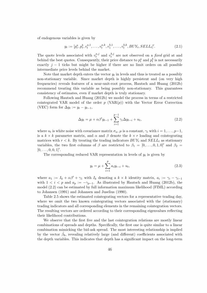
of endogenous variables is given by
yt := [pat , pbt , v
a,1t , . . . , va,kt , vb,11 , . . . , vb,kt , BUYt, SELLt]
′. (2.1)
The quote levels associated with va,jt and vb,jt are not observed on a fixed grid at andbehind the best quotes. Consequently, their price distance to pat and pbt is not necessarilyexactly j − 1 ticks but might be higher if there are no limit orders on all possibleintermediate price levels behind the market.
Note that market depth enters the vector yt in levels and thus is treated as a possiblynon-stationary variable. Since market depth is highly persistent and (on very highfrequencies) reveals features of a near-unit-root process, Hautsch and Huang (2012b)recommend treating this variable as being possibly non-stationary. This guaranteesconsistency of estimates, even if market depth is truly stationary.
Following Hautsch and Huang (2012b) we model the process in terms of a restrictedcointegrated VAR model of the order p (VAR(p)) with the Vector Error Correction(VEC) form for ∆yt := yt − yt−1,
∆yt = µ+ αβ′yt−1 +
p−1∑
i=1
γi∆yt−i + ut, (2.2)
where ut is white noise with covariance matrix σu, µ is a constant, γi with i = 1, . . . , p−1,is a k × k parameter matrix, and α and β denote the k × r loading and cointegratingmatrices with r < k. By treating the trading indicators BUYt and SELLt as stationaryvariables, the two first columns of β are restricted to β1 = [0, . . . , 0, 1, 0]′ and β2 =[0, . . . , 0, 0, 1]′.
The corresponding reduced VAR representation in levels of yt is given by
yt = µ+
p∑
i=1
aiyt−i + ut, (2.3)
where a1 := Ik + αβ′ + γ1 with Ik denoting a k × k identity matrix, ai := γi − γi−1
with 1 < i < p and ap := −γp−1. As illustrated by Hautsch and Huang (2012b), themodel (2.2) can be estimated by full information maximum likelihood (FIML) accordingto Johansen (1991) and Johansen and Juselius (1990).
Table 2.5 shows the estimated cointegrating vectors for a representative trading day,where we omit the two known cointegrating vectors associated with the (stationary)trading indicators and all corresponding elements in the remaining cointegration vectors.The resulting vectors are ordered according to their corresponding eigenvalues reflectingtheir likelihood contributions.
We observe that the first five and the last cointegration relations are mostly linearcombinations of spreads and depths. Specifically, the first one is quite similar to a linearcombination mimicking the bid-ask spread. The most interesting relationship is impliedby the vector β8, revealing relatively large (and different) coefficients associated withthe depth variables. This indicates that depth has a significant impact on the long-term
46
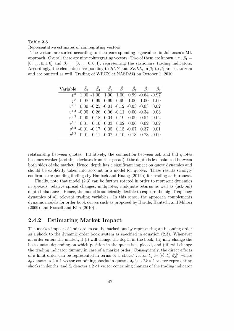
Table 2.5Representative estimates of cointegrating vectorsThe vectors are sorted according to their corresponding eigenvalues in Johansen’s ML
approach. Overall there are nine cointegrating vectors. Two of them are known, i.e., β1 =[0, . . . , 0, 1, 0] and β2 = [0, . . . , 0, 0, 1], representing the stationary trading indicators.Accordingly, the elements corresponding to BUY and SELL, in β3 to β9 are set to zeroand are omitted as well. Trading of WRCX at NASDAQ on October 1, 2010.
Variable β3 β4 β5 β6 β7 β8 β9
pa 1.00 -1.00 1.00 1.00 0.99 -0.64 -0.97pb -0.98 0.99 -0.99 -0.99 -1.00 1.00 1.00
va,1 0.00 -0.25 -0.01 -0.12 -0.03 -0.03 0.02va,2 -0.00 0.26 0.06 -0.11 0.00 -0.34 0.03va,3 0.00 -0.18 -0.04 0.19 0.09 -0.54 0.02vb,1 0.01 0.16 -0.03 0.02 -0.06 0.02 0.02vb,2 -0.01 -0.17 0.05 0.15 -0.07 0.37 0.01vb,3 0.01 0.11 -0.02 -0.10 0.13 0.73 -0.00
relationship between quotes. Intuitively, the connection between ask and bid quotesbecomes weaker (and thus deviates from the spread) if the depth is less balanced betweenboth sides of the market. Hence, depth has a significant impact on quote dynamics andshould be explicitly taken into account in a model for quotes. These results stronglyconfirm corresponding findings by Hautsch and Huang (2012b) for trading at Euronext.
Finally, note that model (2.3) can be further rotated in order to represent dynamicsin spreads, relative spread changes, midquotes, midquote returns as well as (ask-bid)depth imbalances. Hence, the model is sufficiently flexible to capture the high-frequencydynamics of all relevant trading variables. In this sense, the approach complementsdynamic models for order book curves such as proposed by Hardle, Hautsch, and Mihoci(2009) and Russell and Kim (2010).
2.4.2 Estimating Market Impact
The market impact of limit orders can be backed out by representing an incoming orderas a shock to the dynamic order book system as specified in equation (2.3). Wheneveran order enters the market, it (i) will change the depth in the book, (ii) may change thebest quotes depending on which position in the queue it is placed, and (iii) will changethe trading indicator dummy in case of a market order. Consequently, the direct effectsof a limit order can be represented in terms of a ’shock’ vector δy := [δ′p, δ
′v, δ
′d]′, where
δp denotes a 2× 1 vector containing shocks in quotes, δv is a 2k × 1 vector representingshocks in depths, and δd denotes a 2×1 vector containing changes of the trading indicator
47

1
1.51.4
1
1.51.4
price
dep
th0.5
→
1
1.51.4
1.51.51.4
price
dep
th
Figure 2.2 (Scenario 1a (normal limit order)): An incoming buy limit order withprice 1000 and size 0.5. It affects only the depth at the best bid without changing theprevailing quotes or resulting in a trade. Figure from Hautsch and Huang (2012b).
dummy.Following Hautsch and Huang (2012b), we design the impulse response vectors as-
sociated with four scenarios commonly faced by market participants. As graphicallyillustrated by Figures 2.2 to 2.4, a three-level order book is initialized at the best askpat = 1002, best bid pbt = 1000, second best ask 1003, second best bid 999, and depthlevels on the bid side vb,1t = 1, vb,2t = 1.5, vb,3t = vb,4t = 1.4. The following scenarios areconsidered:5
Scenario 1a (normal limit order): arrival of a buy limit order with price 1000 andsize 0.5 to be placed at the market. As shown in Figure 2.2, this order will beconsolidated at the best bid without changing the prevailing quotes. Because theinitial depth on the first level is 1.0, the change of the log depth is ln(1.5) ≈ 0.4.Correspondingly, the shock vectors are given by δv = [0, 0, 0, 0.4, 0, 0]′, δp = δd =[0, 0]′.
Scenario 1b (passive limit order): arrival of a buy limit order with price 999 andsize 0.5 to be posted behind the market. As in the scenario above, it does notchange the prevailing quotes and only affects the depth at the second best bid.We have δv = [0, 0, 0, 0, ln(2)− ln(1.5) ≈ 0.29, 0]′, δp = δd = [0, 0]′.
Scenario 2 (aggressive limit order): arrival of a buy limit order with price 1001 andsize 0.5 to be posted inside of the current spread. Figure 2.3 shows that it improves
5For sake of brevity, the scenarios are only characterized for buy orders. Sell orders areanalyzed accordingly.
48
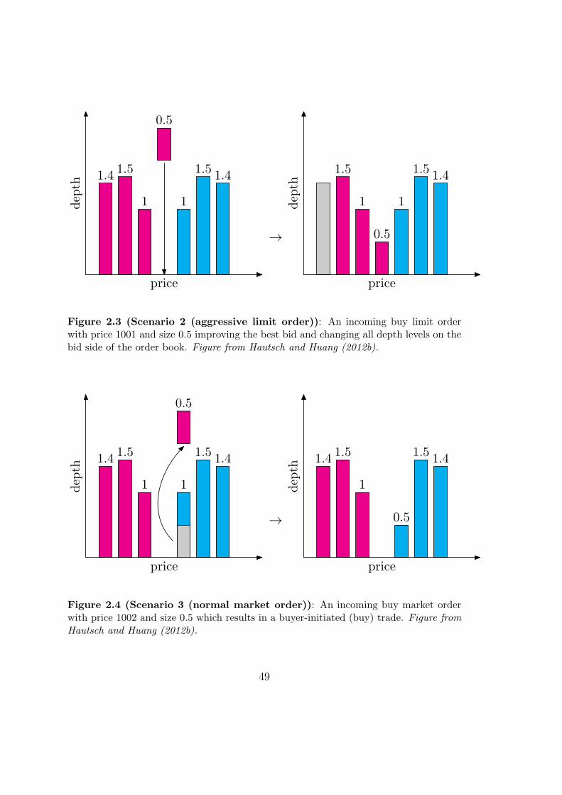
1
1.51.4
1
1.51.4
price
dep
th
0.5
→
1
1.51.4
1
1.5
0.5
pricedep
th
Figure 2.3 (Scenario 2 (aggressive limit order)): An incoming buy limit orderwith price 1001 and size 0.5 improving the best bid and changing all depth levels on thebid side of the order book. Figure from Hautsch and Huang (2012b).
1
1.51.4
1
1.51.4
price
dep
th
0.5
→ 0.5
1.51.4
1
1.51.4
price
dep
th
Figure 2.4 (Scenario 3 (normal market order)): An incoming buy market orderwith price 1002 and size 0.5 which results in a buyer-initiated (buy) trade. Figure fromHautsch and Huang (2012b).
49

Table 2.6Shock vectors implied by the underlying four scenariosInitial order book: best ask pat = 1002, best bid pbt = 1000, second best ask = 1003,
second best bid = 999. Volumes on the ask/bid side: va/b,1t = 1 at the best bid,
va/b,2t = 1.5 at the second best bid, and v
a/b,3t = v
a/b,4t = 1.4 at the third and fourth best
bids, respectively. Notation: δv denotes changes in market depths; δp denotes changes ofthe best bid and best ask; δd denotes changes of the trading indicator variables. Figurefrom Hautsch and Huang (2012b)
Scenario limit order shock vectors(dir,price,size) δ′v δ′p δ′d
‘normal limit order’ (Bid,1000, 0.5) [0, 0, 0, 0.4, 0, 0] [0, 0] [0, 0]‘passive limit order’ (Bid,999, 0.5) [0, 0, 0, 0, 0.29, 0] [0, 0] [0, 0]‘aggressive limit order’ (Bid,1001, 0.5) [0, 0, 0,−0.69,−0.4, 0.07] [0, 0.001] [0, 0]‘normal market order’ (Bid,1002, 0.5) [−0.69, 0, 0, 0, 0, 0] [0, 0] [1, 0]
the best bid by 0.1% and accordingly shifts all depth levels on the bid side. Theresulting shock vector is given by δv = [0, 0, 0, (ln(0.5) ≈ −0.69), (ln(1/1.5) ≈−0.4), (ln(1.5/1.4) ≈ 0.07)]′, δp = [0, 0.001]′ and δd = [0, 0]′.
Scenario 3 (normal market order): arrival of a buy order with price 1002 and size0.5. This order will be immediately executed against standing limit orders at thebest ask quote. Because it absorbs liquidity from the book, it shocks the corre-sponding depth levels negatively. Figure 2.4 depicts the corresponding changes ofthe order book as represented by δv = [ln(0.5) ≈ −0.69, 0, 0, 0, 0, 0]′, δp = [0, 0]′
and δd = [1, 0]′.
Table 2.6 summarizes the shock vectors implied by the illustrating scenarios.The market reactions induced by incoming limit orders are captured by the impulse
response function,
f(h; δy) = E[yt+h|yt + δy, yt−1, · · · ]− E[yt+h|yt, yt−1, · · · ], (2.4)
where the shock on quotes, depths and trading indicators is denoted by δy := [δ′p, δ′v, δ
′d]′
and h is the number of periods (measured in ‘order event time’).Note that the impulse responses need not to be orthogonalized as contemporane-
ous relationships between quotes and depths are captured by construction of the shockvector. Moreover, our data is based on the arrival time of orders avoiding time aggre-gation as another source of mutual dependence in high-frequency order book data. Theimpulse-response function according to equation (2.4) can be written as
f(h; δy) = JAhJ ′δy, (2.5)
50

where
A :=
A1 · · · Ap−1 Ap
IK 0 0. . .
......
0 · · · IK 0
︸ ︷︷ ︸Kp×Kp
.
Given the consistent estimator a for a := vec(A1, . . . , Ap) in (2.3) we have
√T (a− a)
d→ N (0,Σa).
Lutkepohl (1990) shows that the asymptotic distribution of the impulse-response func-tion is given by √
T (f − f)d→ N (0, GhΣaG
′h), (2.6)
where Gh := ∂ vec(f)/∂ vec(A1, · · · , Ap)′. This expression can be explicitly written as
Gh =h−1∑
i=0
(δ′yJ(A
′)h−1−i⊗ JAiJ ′
). (2.7)
The permanent impact of limit order can be deduced from Ganger’s representationof the cointegrated VAR as
f(δy) := limh→∞
f(h; δy) = Cδy, (2.8)
where
C = β⊥
(α′⊥
(IK −
p−1∑
i=1
Γi
)β⊥
)−1
α′⊥ . (2.9)
2.5 Market Impact at NASDAQ
We model the best quotes and market depths up to the third level. Computa-tional burden is reduced by separately estimating the model fore each of the 21trading days. The market impact is then computed as the monthly average ofindividual (daily) impulse response. Likewise, confidence intervals are computedbased on daily averages. For sake of brevity we refrain from presenting all in-dividual results for the ten stocks. We rather illustrate representative evidencebased on Warner Chilcott plc (ticker symbol WCRX) using a cointegrated VAR(10)model. The results for the remaining stocks are provided in a web appendix onhttp://amor.cms.hu-berlin.de/~huangrui/project/order_impact_nasdaq/. In-deed, we find the same pattern as in Hautsch and Huang (2012b).
Figure 2.5 depicts the market impact of buy and sell limit orders posted at the bestquotes as shown in Scenario 1 in Section 2.4.2. The impact starts at zero since sucha limit order does not directly change quotes. As expected, both ask and bid quotes
51
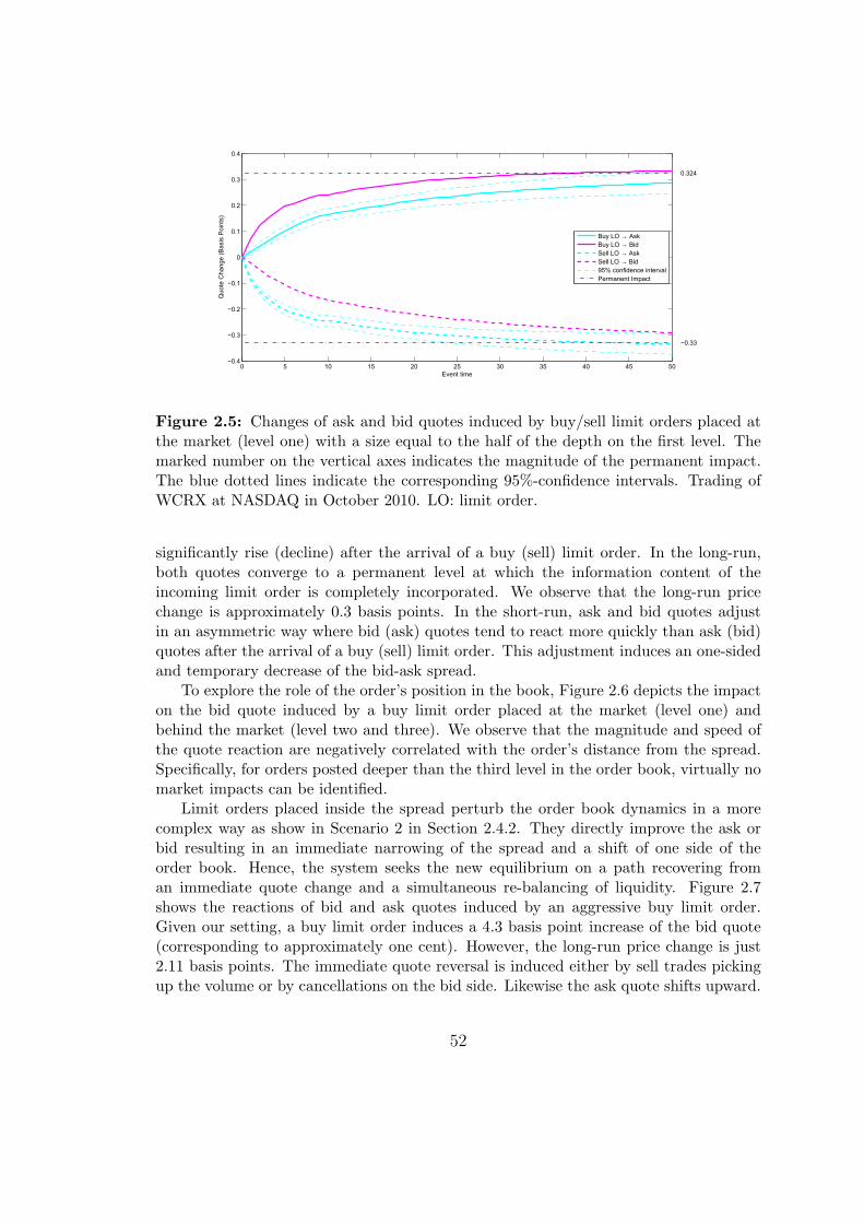
0 5 10 15 20 25 30 35 40 45 50−0.4
−0.3
−0.2
−0.1
0
0.1
0.2
0.3
0.4
0.324
−0.33
Event time
Quo
te C
hang
e (B
asis
Poi
nts)
Buy LO → AskBuy LO → BidSell LO → AskSell LO → Bid95% confidence intervalPermanent Impact
Figure 2.5: Changes of ask and bid quotes induced by buy/sell limit orders placed atthe market (level one) with a size equal to the half of the depth on the first level. Themarked number on the vertical axes indicates the magnitude of the permanent impact.The blue dotted lines indicate the corresponding 95%-confidence intervals. Trading ofWCRX at NASDAQ in October 2010. LO: limit order.
significantly rise (decline) after the arrival of a buy (sell) limit order. In the long-run,both quotes converge to a permanent level at which the information content of theincoming limit order is completely incorporated. We observe that the long-run pricechange is approximately 0.3 basis points. In the short-run, ask and bid quotes adjustin an asymmetric way where bid (ask) quotes tend to react more quickly than ask (bid)quotes after the arrival of a buy (sell) limit order. This adjustment induces an one-sidedand temporary decrease of the bid-ask spread.
To explore the role of the order’s position in the book, Figure 2.6 depicts the impacton the bid quote induced by a buy limit order placed at the market (level one) andbehind the market (level two and three). We observe that the magnitude and speed ofthe quote reaction are negatively correlated with the order’s distance from the spread.Specifically, for orders posted deeper than the third level in the order book, virtually nomarket impacts can be identified.
Limit orders placed inside the spread perturb the order book dynamics in a morecomplex way as show in Scenario 2 in Section 2.4.2. They directly improve the ask orbid resulting in an immediate narrowing of the spread and a shift of one side of theorder book. Hence, the system seeks the new equilibrium on a path recovering froman immediate quote change and a simultaneous re-balancing of liquidity. Figure 2.7shows the reactions of bid and ask quotes induced by an aggressive buy limit order.Given our setting, a buy limit order induces a 4.3 basis point increase of the bid quote(corresponding to approximately one cent). However, the long-run price change is just2.11 basis points. The immediate quote reversal is induced either by sell trades pickingup the volume or by cancellations on the bid side. Likewise the ask quote shifts upward.
52
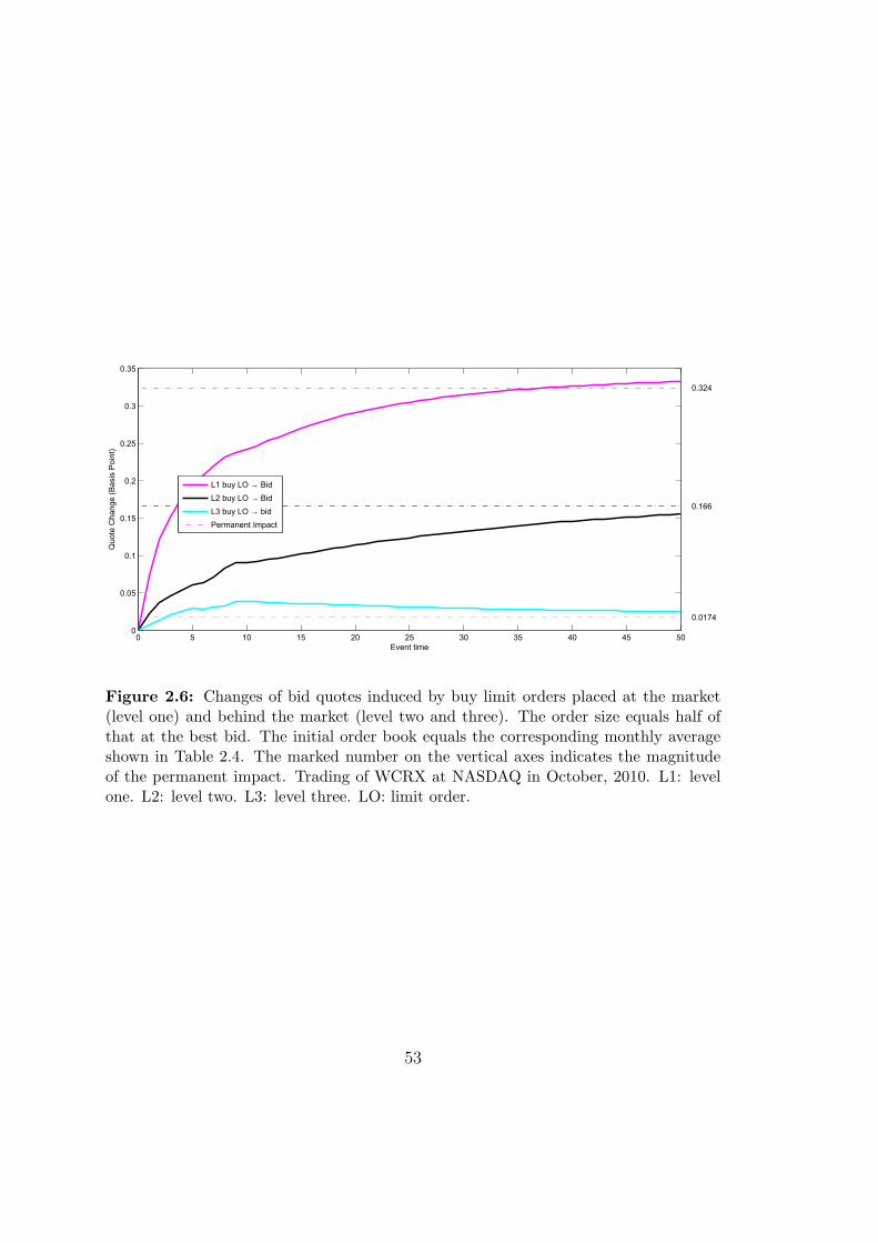
0 5 10 15 20 25 30 35 40 45 500
0.05
0.1
0.15
0.2
0.25
0.3
0.35
0.324
0.166
0.0174
Event time
Quo
te C
hang
e (B
asis
Poi
nt)
L1 buy LO → BidL2 buy LO → BidL3 buy LO → bidPermanent Impact
Figure 2.6: Changes of bid quotes induced by buy limit orders placed at the market(level one) and behind the market (level two and three). The order size equals half ofthat at the best bid. The initial order book equals the corresponding monthly averageshown in Table 2.4. The marked number on the vertical axes indicates the magnitudeof the permanent impact. Trading of WCRX at NASDAQ in October, 2010. L1: levelone. L2: level two. L3: level three. LO: limit order.
53

0 5 10 15 20 250
0.5
1
1.5
2
2.5
3
3.5
4
4.5
2.11
Event time
Quo
te C
hang
e (B
asis
Poi
nt)
Buy LO → AskBuy LO → BidPermanent Impact
0 5 10 15 20 25 30 35 40 45 502
2.5
3
3.5
4
4.5
2.11
3.4
3.95
Event time
Quo
te C
hang
e (B
asis
Poi
nt)
Small buy LO → Bid Mid buy LO → BidBig buy LO → BidPermanent Impact
Figure 2.7: Left: Changes of quotes induced by buy limit orders placed inside of thespread with a size equal to the depth at the bid. Right: Changes of bid quote inducedby buy limit orders placed inside of the spread with different sizes. The initial orderbook equals the corresponding monthly average shown in Table 2.4. Small size: depthat the bid. Mid size: 7 times of the depth at the bid. Big size: 15 times of the depth atthe bid. Trading of WCRX at NASDAQ in October, 2010. LO: limit order.
We hence observe an asymmetric re-balancing of quotes and a corresponding re-wideningof the spread.
The right plot of Figure 2.7 shows how the size of incoming aggressive limit ordersaffects quote reactions. In case of a comparably small order, the posted volume islikely to be quickly picked up or cancelled, shifting back the bid quote. In contrast,large volumes over-bid the prevailing quote causing a significant long-run impact. Thisconfirms findings by Hautsch and Huang (2012b) for Euronext Amsterdam and showsthat aggressive limit orders with large order sizes carry information and serve as pricingsignals.
Figure 2.8 compares the market impact induced by a buy market order and a similarbuy limit order posted at the bid. We observe that both bid and ask quotes sharplyincrease after the arrival of a buy market order. The permanent shift of quotes inducedby a market order is approximately 4 times greater than that by an incoming limitorder. This finding supports theoretical predictions by Rosu (2010). Moreover, in caseof a market order, the ask reacts more quickly than the bid. Hence, we observe anasymmetric adjustment of the two sides of the market resulting in a temporary wideningof spreads.
Since the market impact of limit orders depends not only on the market microstruc-ture but also on the characteristics of the individual stock, an ultimate comparison ofestimated market impacts on NASDAQ with those on Euronext (see Hautsch and Huang(2012b)) is rather difficult. Nevertheless, we do find a significant difference when com-
54

0 5 10 15 20 25 30 350
0.5
1
1.51.46
0.324
Event time
Quo
te C
hang
e (B
asis
Poi
nt)
Buy MO → Ask Buy MO → BidBuy LO → AskBuy LO → BidPermanent Impact
Figure 2.8: Changes of ask and bid quotes induced by a buy market order and a buylimit order of similar size placed at the market. The order size is half of the depth atthe best bid. The initial order book equals the corresponding monthly average shownin Table 2.4. Trading of WCRX at NASDAQ in October, 2010. LO: limit order; MO:market order.
paring the market impact of trades to that of limit orders. While on Euronext Hautschand Huang (2012b) find robust evidence for the market impact of trades trading at bestquotes being approximately four times of the market impact of a limit order of similarsize, this does not necessarily hold for all stocks at NASDAQ, such as, e.g., GOOG,STRA and UTHR. We explain this finding by the existence of hidden liquidity inside ofbid-ask spreads as shown in Table 2.3. When the market participant expects a betterprice than the best quote to be available inside of the spread, she would naturally inter-pret a market order placed at the best quotes as being comparably more aggressive as itwalks through the (hidden) price levels. As a consequence, the reaction to an incomingmarket order becomes stronger. Similarly, an incoming limit order is interpreted as beingcomparably more passive. Consequently, the market impact of limit orders decreases.
2.6 Optimal Order Size
The expected price impact induced by a limit order placement is a key parameter intrading decisions. Therefore, in trading strategies, it might be of particular interestto explicitly control the expected market impact. The estimates of the price impactprovided in the previous section can be used to back out the size of an order (given itsposition in the queue) which is necessary to cause a given expected price impact.
In fact, due to the discreteness of prices, the magnitude of a price impact can be
55
interpreted in a probabilistic context. Given a minimum tick size at equity marketslike NASDAQ, a practitioner who prefers not to shift the price with probability ξ mustdesign the order such that the expected price shift, i.e., the magnitude of the impact, isless than 1−ξ ticks. This is straightforwardly seen by noticing that when the probabilityis exactly ξ, the minimum level of the market impact is
permanent market impact = E[long-run price shift]
= ξ × (0 ticks) + (1− ξ)× (1 ticks)
= 1− ξ (ticks).
(2.10)
In the following we shall illustrate how to explicitly compute the optimal order sizesubject to the given control level ξ. For ease of illustration, consider a bid limit orderwith size m placed at the second best bid. In our setting based on a 3-level order book,it is represented as a 10-dimensional shock vector with only one non-zero element at the9-th row according to the order of variables in equation (2.1),
δ9 = log
(m
depth at second best bid+ 1
).
By equation (2.8), the corresponding permanent impact on the bid is given by
c29 × log
(m
depth at second best bid+ 1
)×[
bid
tick size
], (2.11)
where c29 is the ninth element in the second row of matrix C in (2.9). Plugging (2.11)into (2.10) and solving for m gives
m =
(exp
[(1− ξ)× tick size
bid× c29
]− 1
)× (depth at second best bid). (2.12)
Figure 2.9 depicts the permanent impact on bid prices against order sizes for the tenselected stocks. Each curve in the sub-plots presents the permanent impact induced bythe particular type of bid limit order, i.e., “limit orders placed at the second best bid”,“limit orders placed at the best bid” and “limit orders placed inside of the spread”.The order book is initialized at its average. For the sake of clarity, we change theunit of impacts (on the y−axis) from basis points of bid prices to the number of ticks.Furthermore, the control level ξ is set to 0.9 (corresponding to a permanent marketimpact of 0.1 ticks) represented by the horizontal dashed line. The intersections S1 andS2 correspond to optimal sizes of limit orders placed on the best bid and second bestbid, respectively. For instance, for WCRX and subject to the condition that the marketimpact is less than 0.1 cent, the optimal size for a limit order placed at the best bid isaround 600 shares. Likewise, the optimal size for a limit order placed at the second bidis around 1400 shares.
For the stocks GOOG, UTHR and STRA, we observe that the market impact isso large that the intersection S1 corresponds to an order size of less than 100 shares.
56

100 200 300 400 500 600 700 800 900 1000−0.2
0
0.2
0.4
0.6
0.8
1
1.2
1.4
S1 S2
GOOG: 201010
Order Size
Numb
er of
Ticks
Normal limit orderPassive limit orderAggressive limit order
2000 4000 6000 8000 10000 12000 14000−0.2
0
0.2
0.4
0.6
0.8
1
1.2
S1S2
ADBE: 201010
Order Size
Numb
er of
Ticks
Normal limit orderPassive limit orderAggressive limit order
200 400 600 800 1000 1200 1400 1600 1800 20000
0.1
0.2
0.3
0.4
0.5
0.6
0.7
S1 S2
VRTX: 201010
Order Size
Numb
er of
Ticks
Normal limit orderPassive limit orderAggressive limit order
500 1000 1500 2000 25000
0.1
0.2
0.3
0.4
0.5
0.6
0.7
0.8
S1 S2
WFMI: 201010
Order SizeNu
mber
of Tic
ks
Normal limit orderPassive limit orderAggressive limit order
500 1000 1500 2000 2500 3000 3500 40000
0.1
0.2
0.3
0.4
0.5
0.6
0.7
0.8
0.9
S1 S2
WCRX: 201010
Order Size
Numb
er of
Ticks
Normal limit orderPassive limit orderAggressive limit order
1000 2000 3000 4000 5000 6000 7000 8000−0.2
0
0.2
0.4
0.6
0.8
1
1.2
S1S2
DISH: 201010
Order Size
Numb
er of
Ticks
Normal limit orderPassive limit orderAggressive limit order
100 200 300 400 500 600 700 800 900 10000
0.1
0.2
0.3
0.4
0.5
0.6
0.7
0.8
S1 S2
UTHR: 201010
Order Size
Numb
er of
Ticks
Normal limit orderPassive limit orderAggressive limit order
200 400 600 800 1000 1200 1400 16000
0.1
0.2
0.3
0.4
0.5
0.6
0.7
0.8
0.9
S1 S2
LKQX: 201010
Order Size
Numb
er of
Ticks
Normal limit orderPassive limit orderAggressive limit order
1000 2000 3000 4000 5000 6000 7000 8000−0.2
0
0.2
0.4
0.6
0.8
1
1.2
S1S2
PTEN: 201010
Order Size
Numb
er of
Ticks
Normal limit orderPassive limit orderAggressive limit order
100 200 300 400 500 600 700−0.5
0
0.5
1
1.5
2
S1 S2
STRA: 201010
Order Size
Numb
er of
Ticks
Normal limit orderPassive limit orderAggressive limit order
Figure 2.9: Permanent impacts against order sizes. The impacts are induced by bidorders. The initial order book is set to its monthly average. The order sizes at thex−axis range from 100 shares to 5 times of the depth at the best bid in the initial orderbook . The aggressive (in-the-spread) limit orders improve the bid price by 1 cent. Thehorizontal dashed line presents a subject control level corresponding to a permanentmarket impact of 0.1 cents. Trading of ten selected stocks at NASDAQ in October,2010.
57

We explain this phenomenon by three reasons. First, the depth at the best bid iscomparably small. Therefore, a 100-shares-order is a relatively large order given theavailable liquidity at the market. Second, as shown in Table 2.1, prices of these stocksare relatively high. Consequently, the relative minimum tick size is comparably smallimplying lower costs of front-running strategies. Hence, the high market impact reflects ahigh probability of being affected by front-running. Third, the average absolute spreadin ticks is large. Consequently, there is more room for other market participants toimprove their quotes.
Finally, for some stocks, we observe zero or even negative permanent impacts ofsmall orders placed inside of the spread, as, e.g., GOOG, ADBE, DISH, PTEN andSTRA. This is caused by the effect that small limit orders placed inside of the spreadare mainly submitted by trading algorithms and tend to be canceled very quickly if notgetting executed. In other situations, they might be quickly picked up and trigger otheralgorithms issuing market orders and/or canceling existing limit orders on their ownside.
2.7 Conclusion
In this chapter, we provide new empirical evidence on limit order submissions and marketimpacts in NASDAQ trading. Employing TotalView-ITCH data, we can summarize thefollowing major findings. First, we observe huge numbers of order submissions perday with order sizes clustering around round lots. Second, most of the limit orders arecancelled before getting executed. Cancellation times are hardly greater than one second.Third, the volume-weighted execution time of limit orders is substantially greater thanits median indicating that big limit orders face clearly more execution risk. Finally, weobserve that only very few market orders tend to ’walk through the book’.
We find the short-run and long-run price reactions induced by limit order placementsto be consistent with those found by Hautsch and Huang (2012b) for data stemming fromthe Euronext Amsterdam. This implies that these effects are quite stable across markets,despite of differences in market settings. In particular, we find that incoming limit orderhave significant short-run and long-run effects on ask and bid quotes. Buy (sell) limitorders increase (decrease) both ask and bid quotes while temporarily decreasing bid-ask spreads. Similar but stronger effects are found after arrivals of market orders withtemporary increases of bid-ask spreads. For aggressive limit orders posted in the spreadwe find different effects depending on the order size. While the new quote level causedby a large aggressive order also holds in the long run, this is not true for small orders.Their direct effect on quotes tend to be reversed after a while as the order is pickedup. Moreover, it turns out that only limit orders posted up to the second order levelhave significant market impacts. Orders which are placed even deeper in the book havevirtually no effect on the market. Interestingly, we find that small orders placed insideof the spread cause zero or even negative long-run impacts. We explain this finding bythe existence of trading algorithms which cancel such orders very quickly if they do notget executed.
58

Finally, we illustrate how to use the setup to compute optimal sizes of limit ordersgiven a certain intended price impact. This might be helpful to control the risk in tradingstrategies.
59

60
Chapter 3
Identifying and Analyzing HiddenOrder Placements
This chapter is based on Hautsch and Huang (2012c).
3.1 Introduction
Since the introduction and the growing dominance of electronic trading during thenineties, equity markets have trended toward higher transparency and more disclosureof trading information. However, displayed limit orders reveal trading intentions andmay induce adverse selection effects, picking-off risks and “parasitic trading” (see e.g.,Harris, 1997). Consequently, the question of how much transparency should be optimallyprovided on a market is of ongoing importance. In particular, current developments inequity markets away from full transparency and back toward more opaque market struc-tures made this question again very topical in recent market microstructure research.
In modern trading, traders seek to conceal trading strategies and to avoid adverseprice effects by hiding order sizes. Consequently, reserve (“iceberg”) orders which requireto display only a small fraction of the order size are increasingly popular and can be usedon virtually all major exchanges and trading platforms worldwide. An even more extremeform of reducing pre-trade transparency is to trade in form of non-display (“hidden”)orders which can be entirely hidden. Such orders do not even reveal the posted limitprice and thus act as completely hidden liquidity supply in the order book. While thereare a few empirical studies analyzing iceberg orders (see, e.g., Bessembinder, Panayides,and Venkataraman, 2009; Frey and Sandas, 2009), there is no empirical evidence onnon-display orders. Due to the possibility to also hide the underlying limit price, theyinduce trading and order placement effects which are quite different from those causedby iceberg orders and which have not been not well understood yet. For instance, themost interesting aspect behind hidden orders is that they can be placed inside of thebid-ask spread without affecting visible best ask and bid quotes. In fact, this mechanismcreates enormous order activities in markets as market participants try to “ping” for
61
hidden liquidity inside of the spread by posting corresponding “fleeting orders” whichare canceled a few instants later if they do not get executed.
This chapter aims at shedding light on the use of undisclosed orders in an opaquelimit order market. To our best knowledge, this study is the first one providing empiricalevidence on (entirely) hidden order placements in continuous trading of one of the largestequity markets worldwide. Specifically, using data from the NASDAQ TotalView mes-sage stream allows us to retrieve information on hidden depth. Employing an orderedresponse approach with censoring mechanism yields conditional probabilities of hiddenorder locations given the state of the market and provides insights on the distributionof hidden orders across different price levels. Hence, we perform statistical inference onthe aggressiveness of hidden order placements (e.g., within the spread) and analyze howhidden liquidity submitters balance their risk of non-execution and compete for liquid-ity supply. Our findings based on a wide cross-section of NASDAQ stocks show that“dark” liquidity supply is significantly driven by market conditions and thus predictablein terms of the state of the (displayed) order book. We show that under certain marketconditions, there is significant competition for hidden liquidity supply inducing a clearnarrowing of the “hidden” (and thus effective) bid-ask spread. Conversely, in situationswhere the risk of being picked off becomes high, we observe a significant reduction inhidden order submitters’ aggressiveness. Moreover, we provide novel insights into com-petition for hidden liquidity provision and hidden order placements in the presence ofhigh-frequency trading.
The current tendency of trading platforms toward more opaqueness is observable onall major markets. We can differentiate between three major categories. The first groupof markets, including various non-U.S. markets, such as the London Stock Exchange,Frankfurt Stock Exchange (XETRA), Australian Stock Exchange (ASX), Euronext, theMadrid Stock Exchange and the Toronto Stock Exchange, among others, offer the pos-sibility of posting only iceberg orders (or so-called reserve orders) where the trader isobliged to show only a small proportion (called “peak”) of the posted order size. The sec-ond category of trading platforms allows to use both reserve and hidden orders and thusoffers the option to entirely hide an order. Prominent examples are NASDAQ, the NewYork Stock Exchange (NYSE), BATS (Best Alternative Trading System) – currently thethird largest equity market in the U.S. – and the largest U.S. Electronic CommunicationNetwork (ECN) Direct Edge. According to the report by the Securities and ExchangeCommission (2010), these markets cover approximately 75% of share volume in NationalMarket System (NMS) stocks. The third group of modern trading systems are so-calleddark pools where liquidity supply is hidden and no information on order matching andtrading actions is provided to other market participants.
Recent empirical evidence shows that “dark trading” is not negligible and is in-creasingly popular. For instance, Bessembinder, Panayides, and Venkataraman (2009)report that 44% of order volume is hidden and 18% of incoming orders are reserve or-ders on Euronext Paris. Frey and Sandas (2009) show that reserve orders represent 9%of non-marketable orders with sizes of 12 − 20 times the average in German XETRAtrading. The Securities and Exchange Commission (2010) reports that 32 dark pools
62

1 990
5
10
15
20
25
30
35
40
45
stocks sorted by the average spread
Figure 3.1: Percentage of trading volumes executed against hidden depth for 99 NAS-DAQ stocks representing a wide cross-section of the market. The stocks are sortedaccording to their average bid-ask spreads during the investigation period.
in the U.S. contribute approximately 8% of trading volume in NMS stocks. Figure 3.1shows percentages of trading volume executed against hidden liquidity for 99 NASDAQstocks used in our empirical analysis. Averaged across a wide range of the market, ap-proximately 14% of the share volume originates from hidden depth. However, for somestocks, especially those revealing high spreads, it can be even greater than 40%.
The major motivation for hiding orders is to camouflage trading intention. The latterincreases execution risk as the display of (large) orders may cause impatient traders toretreat (Moinas, 2010) and may lead to higher liquidity competition (Buti and Rindi,2011). Moreover, posting limit orders induces front-running strategies (Harris, 1997),and the risk of adverse selection (“picking off risk”; see Harris, 1996). By hiding an order,execution risks can be reduced, while, on the other hand, the risk of non-execution risesas trading counter parties are not obviously attracted. Moreover, typically, hidden orderslose time priority to displayed orders. Hence, for a hidden order submitter it is crucialto balance the risk of non-execution vs. the risk of adverse selection.
Our empirical methodology is designed to provide insights into these motivations. Toidentify the locations of hidden orders, we employ two approaches. Firstly, we measurehidden order aggressiveness in terms of the distance between the order price and thebest (visible) quote on the own side of the limit order book (LOB). The larger thisdistance the deeper a hidden order is placed within the spread and the higher is the orderaggressiveness. The second approach employs the distance to the best visible quote onthe opposite side of the market. The lower this distance, the lower the transaction costsfor a market order submitter on the opposite side. We show that both distance measures
63

are necessary to fully capture the determinants of hidden order placements. Using thissetup, we analyze whether hidden order placements can be predicted using the observablestate of the limit order book and can be explained by hidden order suppliers’ motivationto balance execution risk and adverse selection risk. In particular, we address the majorresearch questions: (i) Does hidden supply compete with observable order flow? (ii)Is there competition between hidden liquidity? (iii) How does hidden supply react toaggressive “pinging”?
Analyzing hidden order placements for 99 stocks covering a wide cross-section of theNASDAQ market in 2010, we can summarize the following results: First, hidden orderplacements follow trade directions in order to increase execution probabilities and toreduce adverse selection. In particular, market participants submit hidden orders lessaggressively when the price moves in their favorable direction. Second, the “hidden”spread is positively correlated with the observed spread. This is particularly true forstocks with comparably high (average) spreads. Third, there is significant competitionfor the provision of liquidity. This is true for hidden liquidity as traders use more aggres-sive hidden orders after observing competing hidden depth on the own side. Moreover,it is also true for the competition between hidden and disclosed liquidity. The latteris empirically supported by a strong (positive) correlation between undisclosed ordersand the visible depth on the same side of the market. Fourth, hidden order submit-ters become more defensive when high-frequency traders actively “ping” for undisclosedvolume in the spread. Overall, our findings clearly show that hidden orders are placedstrategically to balance non-execution and adverse selection risks.
The remainder of this chapter is organized in the following way: In Section 3.2, wereview the theoretical and empirical studies related to undisclosed orders, and formulateour economic hypotheses. Section 3.3 briefly introduces the market environment, butdiscusses in details on the data construction and descriptive statistics. In Section 3.4,we introduce our econometric model for undisclosed orders. Section 3.5 documents ourempirical findings. Section 3.6 concludes.
3.2 Economic Reasoning of Optimal Order Dis-
play
3.2.1 Theories on Undisclosed Orders
Amajor motivation for posting a limit order is to minimize transaction costs by appropri-ately choosing the limit price and to signal trading intention to other market participantsin order to attract counterparties which might be not in the market yet (according toHarris (1996), so-called “passive traders”). Attracting a counterparty is important toincrease the execution probability and to decrease the execution time of the position.However, signaling trading intention may induce adverse price effects. For instance, ac-cording to Moinas (2010), displaying large orders may cause “defensive” market ordertraders to retreat from the market as soon as they interpret the signal as inside infor-
64

mation. Moreover, “parasitic” traders (Harris, 1997) may exploit the information valueof a big order by using front-running strategies. Finally, posting a limit order inducesthe risk of being picked off and thus adverse selection (Harris, 1996) if price changes arestronger than expected and the order is sold (bought) too cheap (expensive).
Based on these economic reasoning, several theories on the usage of undisclosedorders have been developed. Esser and Monch (2007) propose a static framework inwhich the trader optimizes the peak size and limit price of reserve orders by continuouslymonitoring and balancing exposure risk against execution risk. Moinas (2010) presentsa theoretical model where informed traders, as well as large liquidity traders, use reserveorders to mitigate the information leakage. Cebiroglu and Horst (2011) propose a modelwhere traders decide on the peak size of the iceberg order by accounting for the exposure-induced market impact. Buti and Rindi (2011) present a dynamic framework where thetrader chooses her optimal strategy by simultaneously deciding on trading direction,aggressiveness, size and peak proportion of the order. To our best knowledge, it isthe only theoretical model that explicitly incorporates the possibility of hidden orderplacements into traders’ trading options.
3.2.2 Empirical Evidences on Undisclosed Orders
The empirical literature on reserve orders has been growing remarkably during the lastdecade, partially due to its proliferation in limit order markets and the increasing avail-ability of data. Studying trading on Euronext Paris, Bessembinder, Panayides, andVenkataraman (2009) document that reserve orders induce lower implementation shortfall costs but longer times to fill. De Winne and D’Hondt (2007) examine similar dataand find that the detection of hidden depth increases order aggressiveness on the op-posite side. Fleming and Mizrach (2009) examine data from BrockerTec, the leadinginterdealer ECN for U.S. Treasuries and documenting that the use of reserve ordersvaries considerably with the quantity of hidden depth increasing with price volatility.All studies show that the decision on using reserve orders is strongly related to prevail-ing market conditions, as characterized by the bid-ask spread, order book depth andprevailing volatility.
Studying data from the Australian Stock Exchange (ASX), Aitken, Berkman, andMak (2001) find that reserve orders do not have a different price impact than visiblelimit orders. According to their results, the use of reserve orders increases with volatilityand the average order value, while it decreases in tick size and trading activity. Freyand Sandas (2009) analyze the Deutsche Borse’s trading platform XETRA and showthat the price impact of reserve orders depends on the executed fraction of its size withprofitability increasing in the hidden proportion. Based on data from the Spanish StockExchange Pardo Tornero and Pascual (2007) find no significant price impact associatedwith the execution of hidden parts of reserve orders. These findings support the hypoth-esis that liquidity suppliers use reserve orders to compete for liquidity provision whilepreventing picking-off risks.
Tuttle (2006) shows that overall market depth increased significantly after NASDAQ
65
introduced undisclosed orders. Moreover, they provide evidence for hidden sizes beingpredictive for future market price movements while the visible size conveys only little in-formation. Anand and Weaver (2004) examine the abolition in 1996 and re-introductionin 2002 of reserve orders on the Toronto Stock Exchange and show that the spread andvisible depth remain widely unchanged after both events. However, total depth, in-cluding both visible and hidden volume, significantly increases after the re-introduction.Both studies show that market quality is improved after the introduction of reserveorders and that informed traders tend to use them primarily to reduce the price impact.
3.2.3 Testable Hypotheses
Market microstructure theory (see e.g., Easley, Kiefer, and O’Hara, 1997) suggests thatlarge bid-ask spreads reflect a high uncertainty of liquidity suppliers on the state of themarket and the fundamental value of the asset. If hidden liquidity suppliers are dom-inantly liquidity-motivated, they will be reluctant to submit aggressive hidden ordersinside of the spread as a high uncertainty also implies a high picking-off risk. Conse-quently, hidden depth inside of the spread will decrease if spreads widen. Conversely,for informed market participants who want to camouflage their informational advantage,wider spreads open more room for aggressive hidden order placements. Hence, in such asituation we would expect opposite effects with rising hidden liquidity placed inside thespread. Hence:
Hypothesis 1.A The probability of hidden depth inside the spread decreases with thesize of the spread. (Liquidity traders use hidden orders)
Hypothesis 1.B The probability of hidden depth inside the spread increases with thesize of the spread. (Informed traders use hidden orders)
Traders can use undisclosed orders to compete for the provision of liquidity whilepreventing others from undercutting their orders. Buti and Rindi (2011) demonstratethat undisclosed orders are part of equilibrium strategies of liquidity suppliers. In partic-ular, when the depth on the own side of the market is high, traders prefer to place moreaggressive hidden orders inside of the spread to increase the execution probability. Like-wise, in case of a high depth on the opposite side of the market, hidden order submittersmay place their orders deeply inside the spread in order to “win” the (own-side) compe-tition for liquidity provision and to maximize the execution probability if an impatienttrader from the opposite side posts a market order and crosses the spread. However, thisstrategy implies a high adverse selection risk as a high depth on the opposite side mayreflect significant price pressure. Consequently, aggressive hidden orders placed deeplyinside the spread are likely to be picked up if the price pressure piling up on the oppo-site side materializes. Accordingly, we might expect a(n) reduction (increase) of hiddenorder aggressiveness if hidden order submitters’ exposure to adverse selection risk (riskof non-execution) dominates. Expecting a higher importance of non-execution risk, weformulate the following hypotheses:
Hypothesis 2.A The probability of hidden bid (ask) depth inside spreads increaseswhen the bid (ask) visible depth is thick.
66

Hypothesis 2.B The probability of hidden bid (ask) depth inside spreads increaseswhen the ask (bid) visible depth is thick.
Traders’ order submission strategies depend not only on the current state of thelimit order book but also on recent price movements and trading signals. The dynamicequilibrium model on visible order flow proposed by Parlour (1998) shows a “crowdingout” effect among market orders: the probability of incoming sell (buy) market orders islower after observing a buy (sell) market order which is in line with the well-known strongpersistence in trade directions. This effect implies that visible bid (ask) limit ordershave a higher execution probability after a sell (buy) market order. This hypothesisis supported by Hall and Hautsch (2005) showing that price movements are positively(negatively) correlated with the aggressiveness of visible buy (sell) limit orders. Weexpect that liquidity suppliers take advantage of these trading signals by posting hiddenorders deeper inside the spread and thus increase execution probabilities. However,as argued above, in situations where liquidity suppliers aim at benefiting from pricepressure built up on the opposite side of the market, their exposure to adverse selectionrisk increases, which – in the extreme case – might dominate. A similar scenario arisesin situations of prevailing price changes. Also here, it might be advantageous to placean aggressive hidden ask (bid) order after observing a price increase (decrease) and thusto serve as a counter party if further buy (sell) market orders are expected. Again,a counter-effect arises by an increased picking-off risk. Assuming that traders tend tominimize picking-off risk rather than non-execution risk, we expect hidden bid (ask)depth to decrease (increase) in case of sell (buy) pressure.
Moreover, recent trading and price signals may not only generate activity on theopposite side of the market but may also trigger liquidity competition on the own side. Ifliquidity suppliers expect momentum in prevailing price movements and, according to thecrowding out hypothesis, persistence in trade directions, (hidden) liquidity competitionon the same side should become stronger because liquidity suppliers face a higher risk ofnon-execution. Hence, for order activities on the own side, we expect protection againstnon-execution risk to dominate leading to two testable hypotheses:
Hypothesis 3.A The probability of hidden bid depth inside of the spread decreases(increases) when the prevailing trade is seller (buyer)-initiated. The converse effectapplies for hidden ask depth.
Hypothesis 3.B The aggressiveness of hidden bid depth increases (decreases) whenthe price moves up (down).
Traders’ decision on using undisclosed orders might also depend on the asset’s volatil-ity. Foucault (1999) shows that volatility is an important parameter in order submissionstrategies. Indeed, higher volatility implies higher uncertainty on the value of the assetand thus increases the picking off risk. This mechanism is true for visible orders butshould similarly also apply to hidden orders:
Hypothesis 4 The aggressiveness of hidden depth is negatively correlated with pre-vailing asset price volatility.
Hidden depth is a priori unobservable but is ex post identifiable as soon as it gets
67
executed. This is most clearly seen if a limit order posted inside of the spread getsimmediate execution. Such information gives hidden liquidity providers hints on theprevailing competition for hidden liquidity supply which in turn affects their submissionstrategies. As a result of higher (hidden) liquidity competition, they would post more ag-gressive orders to increase their execution probability. Moreover, Buti and Rindi (2011)show that detections of hidden depth encourage more undisclosed order submissions aslong as picking-off risks (and thus adverse selection risks) do not become too high. Thereasoning is that market participants interpret the detection of hidden volume as a signalof high liquidity demand and compete for supplying it. Accordingly, we postulate thefollowing hypothesis:
Hypothesis 5 The aggressiveness of hidden bid (ask) depth increases after somehidden bid (ask) depth has been executed.
In modern trading, high-frequency trading (HFT) plays an increasingly importantrole (see e.g., Angel, Harris, and Spatt, 2010; Securities and Exchange Commission,2010) and might also influence the supply for hidden liquidity. In fact, HFT algorithmstypically employ directional strategies, such as quote-matching and fast-trading (“scalp-ing”), i.e., the idea to post a limit order in front of some other limit order which isexpected to reveal information and to pick up the mis-priced limit orders quickly wheninformation flows in. To avoid such effects, traders prefer using undisclosed orders. How-ever, some HFT trading algorithms also embed strategies for detecting hidden depth,such as “pinging”, where visible limit orders are posted in the spread in order to testwhether they might get executed. Our empirical results show that such effects createenormous order activities on NASDAQ. Pinging strategies, combined with scalping, in-duce severe picking-off risks for undisclosed orders and may make them quite inefficient.Indeed, Buti and Rindi (2011) theoretically show that when hidden depth can be per-fectly detected there is no ground for traders using undisclosed orders to reduce exposurerisks. Accordingly, we expect that hidden liquidity suppliers become less aggressive ifhigh-frequency traders become very active in the market:
Hypothesis 6 The aggressiveness of hidden depth decreases as HFT activities on theopposite side of the market increase.
In Moinas’s (2010) theoretical framework, informed traders use undisclosed ordersto mitigate information leakage. Typically, information asymmetry is highest during theopening period as overnight information has to be processed. Accordingly, we expecta higher hidden order aggressiveness in this period compared to the rest of the tradingday. Moreover, Esser and Monch (2007) show that traders tend to display more oforder sizes when they approach trading closure. This is driven by the typical desire toclose a position before the end of the trading session. Accordingly, trading intentionsare revealed such that order execution probabilities are increased due to a higher timepriority of visible orders. Buti and Rindi (2011) also argue that reserve orders arepreferable to hidden orders in their framework when the time horizon becomes shorter.This leads to the following hypotheses:
Hypothesis 7.A The aggressiveness of hidden depth is higher during the openinghour.
68

Hypothesis 7.B The aggressiveness of hidden depth is lower during the closure hour.
3.3 Measuring Hidden Order Locations
3.3.1 Institutional Background
As one of the largest electronic limit order markets in the world, the NASDAQ Single-Book platform provides an unified procedure for passing limit orders from ECNs (Brutand INET) and the traditional dealer-quote system. In particular, it treats a marketmaker’s quote as a pair of limit orders on both sides of the market and aggregates theminto a centralized order book. During continuous trading between 9:30 and 16:00 EasternTime, the system matches incoming orders against the best (in term of price) prevailing(possibly undisclosed) orders in the LOB. If there is insufficient volume to fully executethe incoming order, the remaining part will be consolidated into the LOB. Besides limitorders and market orders, NASDAQ provides both reserve orders and hidden orders.1 Asa reward for traders disclosing their orders, the hidden part of undisclosed orders losestime priority compared to visible limit orders or peaks of reserve orders on the sameprice level. Market makers at NASDAQ may also provide hidden depth. The NASDAQStock Market trading rule (NASDAQ, 2008) requires the market maker to display atleast one round lot size. In this case, the market maker’s quotation corresponds to apair of reserve orders.
3.3.2 Data
We conduct our study based on 99 stocks traded on NASDAQ over the period of October2010 corresponding to 21 trading days. To represent a wide cross-section across themarket, we select stocks according to market capitalization. We first rank the 500 biggeststocks according to their market capitalizations recorded in the Center for Research inSecurity Prices (CRSP) database on 30th September 2010. Then, we restrict the sampleby selecting a stock out of every percentile resulting in 99 stocks which are divided intothree equal-size groups according to their average spreads and trade frequencies.
We retrieve historical NASDAQ market conditions from TotalView-ITCH data.NASDAQ TotalViewSM data, surpassing NASDAQ Level 2, is the current standardNASDAQ data feed for displaying the real-time full order book depth for market partic-ipants. Historical data files record rich information on order activities, including limit
1NASDAQ also provides so-called “discretionary orders” with a displayed price and size aswell as a non-displayed discretionary price range. When the discretionary price range is hit bya matching order, the discretionary order converts into an IOC (Immediate or Cancel) marketorder. This order type also allows to hide trading intention. However, we do not considerdiscretionary orders as undisclosed orders because (i) they take liquidity rather than providingit, and (ii) it is very difficult to identify them using TotalView-ITCH data as HFT algorithmsgenerate an enormous number of IOC orders.
69
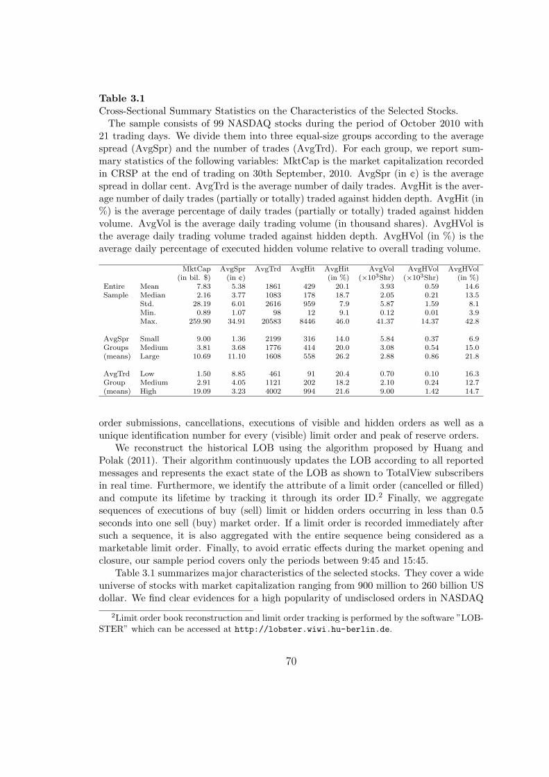
Table 3.1Cross-Sectional Summary Statistics on the Characteristics of the Selected Stocks.The sample consists of 99 NASDAQ stocks during the period of October 2010 with
21 trading days. We divide them into three equal-size groups according to the averagespread (AvgSpr) and the number of trades (AvgTrd). For each group, we report sum-mary statistics of the following variables: MktCap is the market capitalization recordedin CRSP at the end of trading on 30th September, 2010. AvgSpr (in ¢) is the averagespread in dollar cent. AvgTrd is the average number of daily trades. AvgHit is the aver-age number of daily trades (partially or totally) traded against hidden depth. AvgHit (in%) is the average percentage of daily trades (partially or totally) traded against hiddenvolume. AvgVol is the average daily trading volume (in thousand shares). AvgHVol isthe average daily trading volume traded against hidden depth. AvgHVol (in %) is theaverage daily percentage of executed hidden volume relative to overall trading volume.
MktCap AvgSpr AvgTrd AvgHit AvgHit AvgVol AvgHVol AvgHVol(in bil. $) (in ¢) (in %) (×103Shr) (×103Shr) (in %)
Entire Mean 7.83 5.38 1861 429 20.1 3.93 0.59 14.6Sample Median 2.16 3.77 1083 178 18.7 2.05 0.21 13.5
Std. 28.19 6.01 2616 959 7.9 5.87 1.59 8.1Min. 0.89 1.07 98 12 9.1 0.12 0.01 3.9Max. 259.90 34.91 20583 8446 46.0 41.37 14.37 42.8
AvgSpr Small 9.00 1.36 2199 316 14.0 5.84 0.37 6.9Groups Medium 3.81 3.68 1776 414 20.0 3.08 0.54 15.0(means) Large 10.69 11.10 1608 558 26.2 2.88 0.86 21.8
AvgTrd Low 1.50 8.85 461 91 20.4 0.70 0.10 16.3Group Medium 2.91 4.05 1121 202 18.2 2.10 0.24 12.7(means) High 19.09 3.23 4002 994 21.6 9.00 1.42 14.7
order submissions, cancellations, executions of visible and hidden orders as well as aunique identification number for every (visible) limit order and peak of reserve orders.
We reconstruct the historical LOB using the algorithm proposed by Huang andPolak (2011). Their algorithm continuously updates the LOB according to all reportedmessages and represents the exact state of the LOB as shown to TotalView subscribersin real time. Furthermore, we identify the attribute of a limit order (cancelled or filled)and compute its lifetime by tracking it through its order ID.2 Finally, we aggregatesequences of executions of buy (sell) limit or hidden orders occurring in less than 0.5seconds into one sell (buy) market order. If a limit order is recorded immediately aftersuch a sequence, it is also aggregated with the entire sequence being considered as amarketable limit order. Finally, to avoid erratic effects during the market opening andclosure, our sample period covers only the periods between 9:45 and 15:45.
Table 3.1 summarizes major characteristics of the selected stocks. They cover a wideuniverse of stocks with market capitalization ranging from 900 million to 260 billion USdollar. We find clear evidences for a high popularity of undisclosed orders in NASDAQ
2Limit order book reconstruction and limit order tracking is performed by the software ”LOB-STER” which can be accessed at http://lobster.wiwi.hu-berlin.de.
70

Table 3.2Cross-Sectional Summary Statistics on Limit Order Executions and CancellationsThe sample consists of 99 NASDAQ stocks during the period of October 2010, with
21 trading days. We divide them into three equal-size groups according to the averagespread (AvgSpr) and the number of trades (AvgTrd). For each group, we report cross-sectional summary statistics for the following variables: NumLO is the average dailynumber of limit orders (including peaks of reserve orders). NumCanc is the averagedaily number of limit order cancellations before getting (partially) executed. MedCTimis the median of the lifetime of canceled visible limit orders. MedETim is the medianof the lifetime of executed limit orders. VWETim is the volume-weighted executiontime of limit orders. NumALO is the average daily number of limit orders placed insidethe spread (aggressive limit orders). NumACan (in %) is the average daily percentageof cancelled aggressive limit orders placed inside the spread. AvgATim is the averagelifetime of cancelled aggressive limit orders.
NumLO NumCanc MedCTim MedETim VWETim NumALO NumACan AvgATim(×103) (in %) (sec.) (sec.) (sec.) (×103) (in %) (sec.)
Entire Mean 57.92 94.7 9.7 12.9 142.0 3.84 76.3 3.11Sample Median 29.41 94.8 9.2 10.7 103.7 2.52 79.7 2.12
Std. 84.50 1.9 6.3 9.5 152.2 5.81 14.9 4.79Min. 5.01 90.9 0.0 0.8 39.9 0.07 29.4 0.02Max. 650.66 99.2 33.2 60.3 981.2 49.9 98.7 41.0
AvgSpr Small 79.93 93.7 10.0 15.8 154.8 1.85 61.1 1.27Groups Medium 47.14 94.5 11.2 10.6 114.2 4.06 79.6 3.23(means) Large 46.69 95.9 7.8 12.4 156.9 5.62 88.1 4.84
AvgTrd Low 14.67 96.0 12.5 19.9 216.2 2.42 85.1 2.1Group Medium 33.50 94.3 9.3 12.2 109.5 2.50 75.5 2.04(means) High 125.6 93.9 7.2 6.7 100.1 6.61 68.2 5.12
trading. On average, approximately 15% of the trading volume and 20% of all tradesare executed against hidden depth. The average size of executed hidden depth is slightlysmaller than that of visible depth. This is partially due to active HFTs who use high-speed hidden depth detecting algorithms to compete for trading against hidden volume.Moreover, note that only a small proportion of existing hidden depth gets executed (seee.g., Bessembinder, Panayides, and Venkataraman, 2009; Frey and Sandas, 2009). Hence,the share of (undetected) hidden depth is much greater than the magnitudes reportedin the table. Furthermore, we show that the proportion of trading volume executedagainst hidden depth increases as the (average) spread becomes wider. Hence, trades ofhigh-spread stocks are more likely to get price improvements.
Table 3.2 reports summary statistics on limit order executions and cancellations.We find that on average approximately 95% of all limit orders are cancelled withoutgetting (partially) executed. This strikingly high number is robust across the samplewith the cross-sectional standard deviation being very low. In fact, the stock with thesmallest proportion of cancellations still reveals a percentage of 91%. Conversely, weobserve the most extreme situation of a stock revealing 99% cancellations. Moreover,
71

the median lifetime of cancelled orders is less than 10 seconds. For limit orders placedinside the spread, the average time until cancellation is even just around 3 seconds. Thiseffect is obviously driven by a strong influence of HFT-induced pinging strategies aimingat detecting hidden orders inside the spread. Interestingly, large visible limit ordershave much longer execution times than small orders. This is indicated by the volume-weighted execution time of 142 seconds being substantially higher than the medianlifetime of executed limit orders (12.9 seconds). This evidence is in line with extantempirical studies of the market impact of limit orders (see e.g., Eisler, Bouchaud, andKockelkoren, 2011; Hautsch and Huang, 2012b), showing supportive evidence of largetraders’ economic motivation for using undisclosed orders. Finally, cancellation rates ofaggressive limit orders turn out to be lower as they have higher execution probabilities.
3.3.3 Identifying Undisclosed Orders
It is in the nature of things, that information on hidden order placements is not providedby an exchange. Therefore, from classical transaction data sets, as, e.g., the Tradeand Quote (TAQ) database released by the New York Stock Exchange (NYSE), it isimpossible to infer on hidden orders. This difficulty is the major reason for the lackingempirical evidence on hidden order placements. Message data, as provided by TotalView,however, contain information on any activities affecting the visible part of the LOB. Inparticular, it specifically reports executions against hidden orders which allow to identifythe exact position of hidden depth in the LOB. As illustrated below, these details canindeed be utilized to conduct statistical inference on undisclosed order submissions.
In general, we can distinguish between trading scenarios where we can distinctly (expost) identify the location of hidden volume and situations where we can isolate at leastpartial information on the existence of undisclosed volume. Figure 3.2 illustrates anexample of the first scenario where the best (visible) quotes in the LOB are 24.86 (bid)and 24.91 (ask) before a buy limit order with limit price 24.91 is posted. As there is ahidden ask order at price 24.90 inside of the spread, the incoming order is firstly partiallyfilled by this order resulting in a type “P” trade message (denoting executions againsthidden depth in the NASDAQ ITCH 4.0 format). Next, the remaining part of the buyorder is executed against the visible depth at the best ask resulting in an “E” message.Finally, hidden depth at the best (visible) ask gets executed resulting in a further “P”message. The remaining (non-executed) part of the incoming order enters the book asa new buy limit order submission (type “A” message) at 24.91.3
This example shows that due to the existence of hidden depth, the market ordersubmitter faces a better execution price than expected from the visible LOB. If the traderis able to predict the existence of hidden depth within the spread, she can incorporatethese transaction cost savings in her trading strategy. Moreover, it is illustrated that thevisible depth has execution priority over the hidden depth at the same price, no matterwhen the order has been placed. Hence, if further depth on the best ask level cumulates,
3As in general, visible and hidden volumes are provided by more than one order at the sameprice, we typically observe a sequence of simultaneous “P” and “E” messages.
72

Figure 3.2: Left: Stylized trading scenario in a limit order book where a buy marketorder is executed against hidden volume on the ask side and is uniquely identified.Bid orders are marked by green, whereas ask orders are marked by red. All ordersabove the horizontal axis are visible, whereas orders below the axis are hidden. Thenumbered arrows indicate the matching process. Right: Sequence of generated messages(in NASDAQ ITCH 4.0 format) resulting from this transaction.
the time-to-fill of any hidden order becomes longer. Finally, since the execution of thehidden part is uniquely identified, we can exactly locate the undisclosed order in thisexample.
Figure 3.3 shows a scenario which allows to extract at least incomplete informationon hidden order placements. Suppose a buy limit order is submitted inside of the spreadwith price 24.88. The fact that the limit order does not get executed (otherwise we wouldhave been observed a ”P” message), reflects that there cannot be any hidden ask volumeposted on a price level lower than 24.89. Hence, this observation reveals informationabout non-existence of hidden depth. We refer to such an observation as censored as itonly provides a lower (upper) bound for the location of hidden ask (bid) volume.
Finally, as illustrated by Figure 3.4, there might be a scenario where a marketableorder is executed against two (or several) levels of visible depth. The fact that not even apart of the order is executed against hidden volume indicates the non-existence of hiddenask depth on any level up to (including) price level 24.90. Hence, also this observationis censored in the sense that it only yields a location bound.
Summarizing, we infer price information on undisclosed orders based on the followingthree scenarios:
1. Submission of a marketable order when the spread is larger than 1 tick. If theorder gets executed at a price better than the corresponding best (visible) quote,we can exactly identify the hidden order location and thus obtain an “uncensored”observation.
73
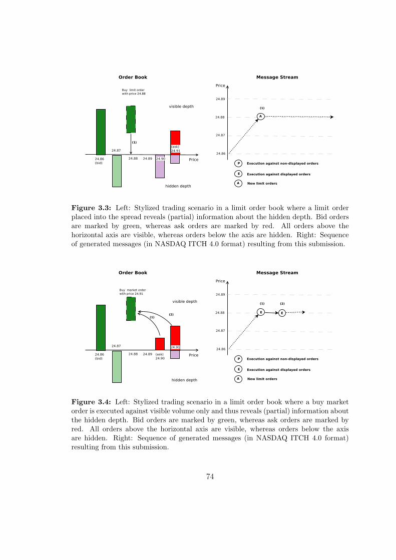
Figure 3.3: Left: Stylized trading scenario in a limit order book where a limit orderplaced into the spread reveals (partial) information about the hidden depth. Bid ordersare marked by green, whereas ask orders are marked by red. All orders above thehorizontal axis are visible, whereas orders below the axis are hidden. Right: Sequenceof generated messages (in NASDAQ ITCH 4.0 format) resulting from this submission.
Figure 3.4: Left: Stylized trading scenario in a limit order book where a buy marketorder is executed against visible volume only and thus reveals (partial) information aboutthe hidden depth. Bid orders are marked by green, whereas ask orders are marked byred. All orders above the horizontal axis are visible, whereas orders below the axisare hidden. Right: Sequence of generated messages (in NASDAQ ITCH 4.0 format)resulting from this submission.
74

Figure 3.5: Graphical illustration of the hidden order aggressiveness measure s andcorresponding classifications for the case of large-spread stocks (4 categories).
2. Submission of a limit order inside of the spread. If it is not executed, we certainlyknow that there is undisclosed order with better limit price. This results into a“censored” observation.
3. Submission of a marketable order with size greater than the depth at the corre-sponding best (visible) quote. As this order may be split across several levels,we can infer on hidden depth at- or behind-the-market. The observation can beuncensored or censored depending on whether it is partially filled by hidden depthor not.
3.3.4 Measuring the Aggressiveness of Undisclosed Orders
Biais, Hillion, and Spatt (1995) classify the aggressiveness of a limit order by measuringits (price) distance to the prevailing best quotes. This scheme has been widely employedin the empirical literature on limit orders (e.g. Griffiths, Smith, Turnbull, and White,2000) and reserve orders (e.g., Bessembinder, Panayides, and Venkataraman, 2009).Accordingly, we measure the aggressiveness of undisclosed orders in a similar way. Inparticular, we measure distances of hidden order placements relative to best quotes onthe own and opposite side of the market.
Let pa and pb denote the best ask and bid quote and po represents the limit price
75

of the undisclosed order. According to our first scheme, we measure the distance of theundisclosed order to the best quote on the order’s own side,
s =
po − pb for undisclosed buy orders,
pa − po for undisclosed sell orders.
Hence, the larger s, the deeper the order is placed in the spread. Conversely, if s ≤ 0, theundisclosed order is placed in the book and can be either a reserve order or a hidden order.Accordingly, s measures aggressiveness from the liquidity supplier’s perspective. Due tothe fact that most observations only reveal incomplete, i.e. “censored”, information, it ismost natural to measure hidden order aggressiveness in terms of categories. As discussedin the following sections, this allows for straightforward and computationally tractableeconometric modelling avoiding severe assumptions on the functional form. Dependingon the underlying (average) size of the spread, we choose different categorization schemes.In particular, we divide the set of hidden order locations into 2, 3 and 4 categories forsmall-spread, medium-spread and large-spread stocks, respectively. Table 3.3 gives thechosen categories depending on s. The choice of the groups is motivated by the need tohave a sufficient number of observations in each category and to use a preferably finecategorization within the spread. Figure 3.5 illustrates the resulting scheme for the caseof large-spread stocks.
As bid-ask spreads are not constant over time, the distance measure s is not sufficientto fully capture hidden order locations. It is rather necessary to measure orders’ aggres-siveness also in terms of the distance to the opposite side of the market. Accordingly,
d =
pa − po for undisclosed buy orders,
po − pb for undisclosed sell orders.
Hence, d represents undisclosed orders’ aggressiveness from the liquidity demander’sperspective, see Figure 3.6. The smaller d, the lower the actual transaction costs for amarket order submitter who gets executed against this undisclosed order. Note that dcannot become negative as any placement behind the opposite side of the market wouldimmediately result into an execution. As shown by Table 3.3, we categorize d in a similarway to s. However, as d highlights the implied transaction costs induced by executionagainst undisclosed orders, we choose a categorization which is particularly fine close tothe opposite side.
Note that the categorizations underlying the two measures can be partially over-lapping. For instance, category 2 in Figure 3.5 overlaps with the categories 1 and 2 inFigure 3.6, while category 3 in Figure 3.6 overlaps with categories 3 and 4 in Figure 3.5.As shown in the empirical part of this chapter, this overlapping structure is particu-larly advantageous as it enables us to capture manifold changes of the hidden depthdistribution by means of relatively simple and robust models.
Table 3.3 summarizes information on undisclosed orders. Firstly, the number oforder submissions revealing hidden depth information is huge, especially for large-spreadstocks. For these stocks, we observe on average approximately 113, 000 submissions.
76

Figure 3.6: Graphical illustration of the hidden order aggressiveness measure d andcorresponding classifications for the case of large-spread stocks (4 categories).
77

Table 3.3Cross-sectional summary statistics on observations on undisclosed ordersThe sample consists of 99 NASDAQ stocks during the period of October 2010 with
21 trading days. We divide them into three equal-size groups according to the averagespread. The aggressiveness of undisclosed orders is measured by s and d as describedin Section 3.3.4. We employ two, three and four categories for small-spread, medium-spread and large-spread stocks, respectively. Censored observations are defined as inSection 3.3.3. For each group we show cross-sectional statistics on total numbers (overall trading days).
Cate- Distance # Observation (×103) Censored Obs. (%) % Buy Orders (%)gory (ticks) max. mean min. max. mean min. max. mean min.Aggressiveness measured by the distance to the own side quote (s)Spread group: small“1” st > 0 147.65 29.32 1.71 96.5 83.3 26.2 52.7 49.8 45.5“2” st ≤ 0 15.33 3.42 0.46 50.6 19.9 5.5 62.7 50.2 43.3
Spread group: medium“1” st > 1 357.27 50.02 7.20 98.8 96.0 92.6 57.0 50.0 44.1“2” st = 1 91.33 21.22 3.91 97.0 87.1 65.1 56.9 49.9 44.2“3” st ≤ 0 63.17 7.895 1.12 83.3 65.0 41.2 58.4 48.5 43.6
Spread group: large“1” st > 3 623.82 76.58 12.13 99.8 97.8 90.6 56.1 50.5 44.7“2” st = 2, 3 193.84 17.04 0.40 98.6 86.4 38.2 56.8 51.2 47.7“3” st = 1 107.46 9.48 0.33 90.2 64.7 23.0 56.0 49.0 43.6“4” st ≤ 0 121.38 10.03 0.77 94.9 81.3 60.0 57.3 49.3 42.1
Aggressiveness measured by the distance to the opposite side quote (d)Spread group: small“1” dt = 1 156.96 31.12 2.07 94.1 75.2 22.4 54.4 49.8 45.1“2” dt > 1 15.19 1.62 0.10 98.0 87.5 69.6 71.5 51.3 37.2
Spread group: medium“1” dt = 1 327.35 57.75 9.89 97.5 93.2 86.3 55.6 50.0 45.0“2” dt = 2 80.48 11.27 1.97 95.8 88.1 77.9 54.9 48.9 40.9“3” dt > 2 99.99 10.11 0.94 93.7 81.3 52.5 61.0 50.4 39.2
Spread group: large“1” dt = 1 561.97 61.63 12.96 99.8 97.2 92.1 55.4 50.4 42.5“2” dt = 2 174.53 17.44 2.89 99.7 93.9 82.7 55.8 50.0 39.6“3” dt = 3, 4 162.94 16.73 1.51 99.3 89.6 68.4 56.3 49.9 41.1“4” dt > 4 147.06 17.34 0.64 98.0 82.0 46.4 77.4 52.0 41.7
78

Table 3.4Definitions of LOB control variables hidden orders on the buy side“Aggressive limit orders” are defined as limit orders undercutting the prevailing best
quote. “Fleeting orders” are defined as limit orders that are canceled within one secondafter the submission.
SPR ≡ log(best ask/best bid)DPO ≡ log(depth at best bid)DPG ≡ log(depth at best ask)TY P ≡ 1 if the prevailing trade is seller-initiated; −1 otherwiseRET ≡ log return over the prevailing 5 minutesV OL ≡ market price range (maximum - minimum) over the prevailing 5 minutesHV O ≡ log(1+volume of executed hidden bid depth during the prevailing 1
minute)HV O5≡ log(1+volume of executed hidden bid depth during the prevailing 5
minutes)HRO ≡ HV O −HV O5
HVG ≡ log(1+volume of executed hidden ask depth during the prevailing 1minute)
HVG5≡ log(1+volume of executed hidden ask depth during the prevailing 5minutes)
HRG ≡ HVG−HVG5
ALO ≡ log(1+ number of aggressive buy limit orders that are not canceled duringthe prevailing 3 minutes)
ALG ≡ log(1+ number of aggressive sell limit orders that are not canceled duringthe prevailing 3 minutes)
HFO ≡ log(1+ number of fleeting buy orders during the prevailing 3 minutes)HFG ≡ log(1+ number of fleeting sell orders during the prevailing 3 minutes)OPN ≡ 1 trading before 10 : 30; 0, otherwise.CLS ≡ 1 trading after 15 : 00; 0, otherwise.
Secondly, more than 90% of all observations are censored in the sense of reflecting onlythe upper bound of aggressiveness of hidden depth. Thirdly, the number of observationson the buy and sell side are very similar.
Finally, note that we label the underlying categories in a consistent way with theleast aggressive categories being associated with the highest label and the most aggressivecategory being associated with the lowest label.
79

3.3.5 Capturing Market Conditions
To test our postulated hypotheses and to relate the usage of undisclosed orders to pre-vailing market conditions, we construct different variables representing various states ofthe market. Table 3.4 gives the exact definitions of constructed variables used for hiddenorder submissions on the buy side.
For statistical inference on the sell side, we modify some of the variables as follows:DPO ≡ log(depth at best ask)DPG ≡ log(depth at best bid)TY P ≡ 1 if the prevailing trade is buyer-initiated; −1 otherwiseRET ≡ negative log return over the prevailing 5 minutesHV O ≡ log(1+volume of executed hidden ask depth during the prevailing 1 minute)HV O5≡ log(1+volume of executed hidden ask depth during the prevailing 5
minutes)HVG ≡ log(1+volume of executed hidden bid depth during the prevailing 1 minute)HVG5≡ log(1+volume of executed hidden bid depth during the prevailing 5
minutes)ALO ≡ log(1+ number of aggressive sell limit orders that are not canceled during
the prevailing 3 minutes)ALG ≡ log(1+ number of aggressive buy limit orders that are not canceled during
the prevailing 3 minutes)HFO ≡ log(1+ number of fleeting sell orders during the prevailing 3 minutes)HFG ≡ log(1+ number of fleeting buy orders during the prevailing 3 minutes)
The prevailing LOB state is represented by the visible bid-ask spread (SPR), reflect-ing the transaction costs of immediate trading, the visible depth on the best level on theown side (DPO) and the visible depth on the best level on the opposite side (DPG).To capture the impact of prevailing trade signals, we include a dummy variable (TY P )representing the most recent trading direction and the prevailing five-minute mid-quotereturn (RET ) capturing short-term price movements. Moreover, local price volatility(V OL) is included in terms of the (max/min) range of trade prices during the last 5minutes. Information on hidden depth is incorporated by the short-run executed hiddendepth on the own side and the opposite side (HV O, HVG), representing how successfullytraders have detected pending hidden depth. Moreover, to assess the relative intensityof temporary hidden order executions, we compute the executed hidden depth duringthe last minute relative to that executed during the last five minutes (HRO, HRG).Moreover, HFT activities are captured by two variables, HFO and HFG, which are thenumber of fleeting orders on the own side and the opposite side, respectively. Defined asin Hasbrouck and Saar (2009), a “fleeting order” is a limit order that is canceled withinone second after the submission and thus is posted to “test” for the existence of hiddenvolume. Using the intensity of fleeting orders as a proxy for HFT activities is inspired byHendershortt, Jones, and Menkveld (2010). To differentiate between fleeting orders and“normal” limit orders, we also include the number of aggressive limit orders that havenot been canceled (ALO, ALG) and thus represent the frequency of quote updating by
80
low frequency traders. Finally, OPN and CLS are dummy variables representing theopening and closure period. To be able to aggregate estimates across the market, allvariables (expect for dummies, i.e., TY P , OPN and CLS) are normalized to have zeromean and unit standard deviation.
3.4 Econometric Modelling
The chosen categorizations straightforwardly motivate modeling hidden order locationsbased on an ordered response model. This has several advantages: Firstly, censored ob-servations are straightforwardly taken into account. Secondly, relating market conditionvariables (as constructed in the previous section) to order categories rather than to plaindistances s and d, requires imposing less assumptions on functional form (e.g., linearity)and allows reducing the impact of extreme observations (e.g., executions against hiddendepth deep in the book). Thirdly, given the high number of observations (combinedwith a significant cross-sectional dimension), a reduction of the computational burdenis crucial to make the approach tractable. In fact, exploiting the Gaussianity and globalconcavity of objective functions in an ordered probit model allows to significantly re-duce computation time in contrast to, for instance, a (censored) count data model (e.g.,negative binomial model) for the variables s or d.
Therefore, we propose modelling hidden order placements using a censored orderedprobit model. In order to test our hypotheses, it is sufficient to utilize only order messageswhich provide information (censored or non-censored) on the location of undisclosedvolume. Consequently, the model is not estimated based on the continuous time seriesof all order book messages but only based on the observations revealing hidden orderinformation. In this sense, we do not require a dynamic (e.g., autoregressive) approachas all information on the current and prevailing state of the market is captured bycorresponding regressors.
3.4.1 An Ordered Probit Model with Censoring
Let yt denote the discrete ordered label representing the underlying categories of undis-closed order placements as described in Section 3.3.4. It is driven by a continuous latentvariable y∗t with the link function given by
yt =
1, if y∗t ≤ γ1
2, if γ1 < y∗t ≤ γ2...
J − 1, if γJ−2 < y∗t ≤ γJ−1
J, if γJ−1 < y∗t
(3.1)
where J is the number of categories and γj , j = 1, . . . , J−1 denote unknown thresholds.Furthermore, y∗t is given by
y∗t = β′xt + εt (3.2)
81

with xt being a (K × 1) vector of regressors as defined in Section 3.3.5, β is a vector ofunknown parameters and εt denotes an i.i.d. standard normally distributed variable. Ifthe response variable yt is observed (i.e., non-censoring), the likelihood function is givenby
LUt =
Φ(γ1 − β′xt) if yt = 1,
Φ(γj − β′xt)− Φ(γj−1 − β′xt) if yt ∈ 2, . . . , j, . . . , J − 1,1− Φ(γJ−1 − β′xt) if yt = J ,
(3.3)
where Φ(·) denotes the cumulative density function of the standard normal distribution.In cases, where yt is not directly observable but only a censored outcome yt related toyt (according to the scenarios described in Figure 3.3 and 3.4) by
yt = j, if yt ∈ j + 1, . . . , J, (3.4)
the likelihood function is given by
LCt =
1− Φ(γj − β′x) if yt = j and j = 1, . . . , J − 2,
1− Φ(γJ−1 − β′x) if yt ≥ J − 1.(3.5)
Hence, the resulting log likelihood function is given by
l =∑
t∈ζU
log(LUt ) +
∑
t∈ζC
log(LCt ), (3.6)
where ζU and ζC denote the index sets of uncensored and censored observations, respec-tively.
The marginal effects of the regressors are straightforwardly given by
q1 =∂F1
∂x= −φ(γ1 − β′x)β,
q2 =∂F2
∂x= −(φ(γ2 − β′x)− φ(γ1 − β′x))β,
...
qJ =∂FJ
∂x= φ(γJ−1 − β′x)β,
(3.7)
which are commonly evaluated at the sample mean x.In case of the dummy variables xd, we compute the marginal effects as
∆Fj = P(y = j|x(xd=1),γ,β)− P(y = j|x(xd=0),γ,β), (3.8)
where x(xd=i) is a vector with the dummy variable xd set to i and all other elements
being equal to x. Appendix B.1 gives the asymptotic distribution of qj and ∆Fj , themaximum likelihood estimator for qj and ∆Fj , respectively.
82

3.4.2 Cross-Sectional Aggregation
We estimate the econometric model on a stock-by-stock basis. For the sake of brevity andcompactness of presentation, we aggregate the corresponding estimates across stocks. Toexplicitly account for differences in estimation precision, we assess the cross-sectional sta-tistical significance relying on a Bayesian framework attributable to DuMouchel (1994)and further implemented by Bessembinder, Panayides, and Venkataraman (2009). As-sume that a parameter estimate associated with stock i, βi, is normally distributed with
βi ∼ i.i.d.N(βi, s2i )
andβi ∼ i.i.d.N(β, σ2),
where s2i is the estimated variance of parameter i and variances σ2 are estimated bymaximum likelihood. Then, the aggregated estimate β is obtained by summing up theweighted estimates for all stocks as
β =N∑
i=1
wiβi, wi =(s2i + σ2)−1
∑Nj=1(s
2j + σ2)−1
. (3.9)
Assuming independence across stocks, the variance of the aggregated estimate is givenby
var(β) =1
∑Nj=1(s
2j + σ2)−1
.
3.5 Empirical Evidence
We estimate separate models for both ask and bid hidden orders for categorizations basedon both distance measures s and d. Hence, covering 99 stocks over the cross-section of themarket, we estimate 396 models in total. Table 3.5 presents the ordered probit estimatesaggregated across all stocks. Recall that lower category labels are associated with ahigher hidden order aggressiveness, thus negative coefficients reflect that undisclosedorders are set (marginally) deeper in the spread. To assess the explanatory power, wereport the pseudo-R2 proposed by McKelvey and Zaviona (1975),
R2MZ =
∑Tt=1(y
∗t − y∗)2
∑Tt=1(y
∗t − y∗)2 + T
(3.10)
where y∗t is the fitted value of the latent variable y∗t with ML estimate of β and y∗ =1/T
∑Tt=1 y
∗t .
Moreover, to provide also insights into the cross-sectional variation of estimates weshow histograms of the significant estimates (5% significance level) in Figures B.1 toB.4 in Appendix B.2. Note that the Bayesian cross-sectional aggregates, as discussed in
83
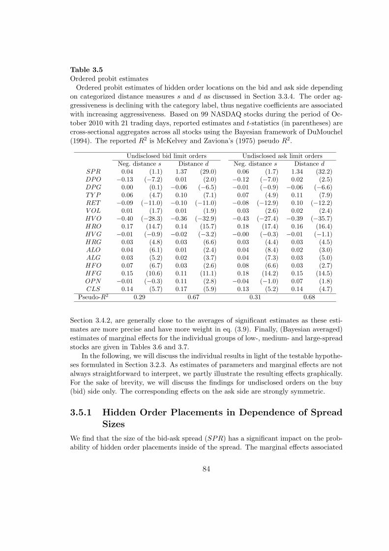
Table 3.5Ordered probit estimatesOrdered probit estimates of hidden order locations on the bid and ask side depending
on categorized distance measures s and d as discussed in Section 3.3.4. The order ag-gressiveness is declining with the category label, thus negative coefficients are associatedwith increasing aggressiveness. Based on 99 NASDAQ stocks during the period of Oc-tober 2010 with 21 trading days, reported estimates and t-statistics (in parentheses) arecross-sectional aggregates across all stocks using the Bayesian framework of DuMouchel(1994). The reported R2 is McKelvey and Zaviona’s (1975) pseudo R2.
Undisclosed bid limit orders Undisclosed ask limit ordersNeg. distance s Distance d Neg. distance s Distance d
SPR 0.04 (1.1) 1.37 (29.0) 0.06 (1.7) 1.34 (32.2)DPO −0.13 (−7.2) 0.01 (2.0) −0.12 (−7.0) 0.02 (2.5)DPG 0.00 (0.1) −0.06 (−6.5) −0.01 (−0.9) −0.06 (−6.6)TY P 0.06 (4.7) 0.10 (7.1) 0.07 (4.9) 0.11 (7.9)RET −0.09 (−11.0) −0.10 (−11.0) −0.08 (−12.9) 0.10 (−12.2)V OL 0.01 (1.7) 0.01 (1.9) 0.03 (2.6) 0.02 (2.4)HV O −0.40 (−28.3) −0.36 (−32.9) −0.43 (−27.4) −0.39 (−35.7)HRO 0.17 (14.7) 0.14 (15.7) 0.18 (17.4) 0.16 (16.4)HVG −0.01 (−0.9) −0.02 (−3.2) −0.00 (−0.3) −0.01 (−1.1)HRG 0.03 (4.8) 0.03 (6.6) 0.03 (4.4) 0.03 (4.5)ALO 0.04 (6.1) 0.01 (2.4) 0.04 (8.4) 0.02 (3.0)ALG 0.03 (5.2) 0.02 (3.7) 0.04 (7.3) 0.03 (5.0)HFO 0.07 (6.7) 0.03 (2.6) 0.08 (6.6) 0.03 (2.7)HFG 0.15 (10.6) 0.11 (11.1) 0.18 (14.2) 0.15 (14.5)OPN −0.01 (−0.3) 0.11 (2.8) −0.04 (−1.0) 0.07 (1.8)CLS 0.14 (5.7) 0.17 (5.9) 0.13 (5.2) 0.14 (4.7)
Pseudo-R2 0.29 0.67 0.31 0.68
Section 3.4.2, are generally close to the averages of significant estimates as these esti-mates are more precise and have more weight in eq. (3.9). Finally, (Bayesian averaged)estimates of marginal effects for the individual groups of low-, medium- and large-spreadstocks are given in Tables 3.6 and 3.7.
In the following, we will discuss the individual results in light of the testable hypothe-ses formulated in Section 3.2.3. As estimates of parameters and marginal effects are notalways straightforward to interpret, we partly illustrate the resulting effects graphically.For the sake of brevity, we will discuss the findings for undisclosed orders on the buy(bid) side only. The corresponding effects on the ask side are strongly symmetric.
3.5.1 Hidden Order Placements in Dependence of SpreadSizes
We find that the size of the bid-ask spread (SPR) has a significant impact on the prob-ability of hidden order placements inside of the spread. The marginal effects associated
84
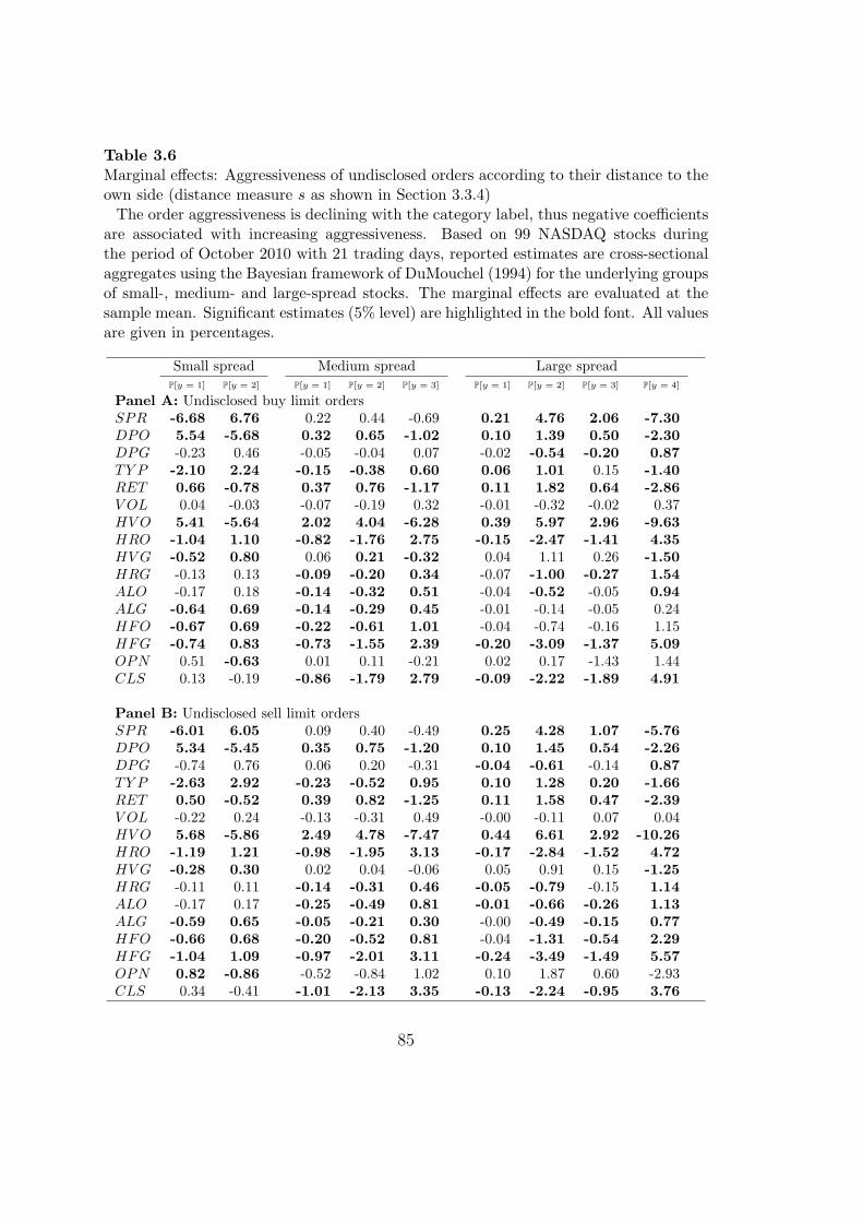
Table 3.6Marginal effects: Aggressiveness of undisclosed orders according to their distance to theown side (distance measure s as shown in Section 3.3.4)The order aggressiveness is declining with the category label, thus negative coefficients
are associated with increasing aggressiveness. Based on 99 NASDAQ stocks duringthe period of October 2010 with 21 trading days, reported estimates are cross-sectionalaggregates using the Bayesian framework of DuMouchel (1994) for the underlying groupsof small-, medium- and large-spread stocks. The marginal effects are evaluated at thesample mean. Significant estimates (5% level) are highlighted in the bold font. All valuesare given in percentages.
Small spread Medium spread Large spreadP[y = 1] P[y = 2] P[y = 1] P[y = 2] P[y = 3] P[y = 1] P[y = 2] P[y = 3] P[y = 4]
Panel A: Undisclosed buy limit ordersSPR -6.68 6.76 0.22 0.44 -0.69 0.21 4.76 2.06 -7.30DPO 5.54 -5.68 0.32 0.65 -1.02 0.10 1.39 0.50 -2.30DPG -0.23 0.46 -0.05 -0.04 0.07 -0.02 -0.54 -0.20 0.87TY P -2.10 2.24 -0.15 -0.38 0.60 0.06 1.01 0.15 -1.40RET 0.66 -0.78 0.37 0.76 -1.17 0.11 1.82 0.64 -2.86V OL 0.04 -0.03 -0.07 -0.19 0.32 -0.01 -0.32 -0.02 0.37HV O 5.41 -5.64 2.02 4.04 -6.28 0.39 5.97 2.96 -9.63HRO -1.04 1.10 -0.82 -1.76 2.75 -0.15 -2.47 -1.41 4.35HVG -0.52 0.80 0.06 0.21 -0.32 0.04 1.11 0.26 -1.50HRG -0.13 0.13 -0.09 -0.20 0.34 -0.07 -1.00 -0.27 1.54ALO -0.17 0.18 -0.14 -0.32 0.51 -0.04 -0.52 -0.05 0.94ALG -0.64 0.69 -0.14 -0.29 0.45 -0.01 -0.14 -0.05 0.24HFO -0.67 0.69 -0.22 -0.61 1.01 -0.04 -0.74 -0.16 1.15HFG -0.74 0.83 -0.73 -1.55 2.39 -0.20 -3.09 -1.37 5.09OPN 0.51 -0.63 0.01 0.11 -0.21 0.02 0.17 -1.43 1.44CLS 0.13 -0.19 -0.86 -1.79 2.79 -0.09 -2.22 -1.89 4.91
Panel B: Undisclosed sell limit ordersSPR -6.01 6.05 0.09 0.40 -0.49 0.25 4.28 1.07 -5.76DPO 5.34 -5.45 0.35 0.75 -1.20 0.10 1.45 0.54 -2.26DPG -0.74 0.76 0.06 0.20 -0.31 -0.04 -0.61 -0.14 0.87TY P -2.63 2.92 -0.23 -0.52 0.95 0.10 1.28 0.20 -1.66RET 0.50 -0.52 0.39 0.82 -1.25 0.11 1.58 0.47 -2.39V OL -0.22 0.24 -0.13 -0.31 0.49 -0.00 -0.11 0.07 0.04HV O 5.68 -5.86 2.49 4.78 -7.47 0.44 6.61 2.92 -10.26HRO -1.19 1.21 -0.98 -1.95 3.13 -0.17 -2.84 -1.52 4.72HVG -0.28 0.30 0.02 0.04 -0.06 0.05 0.91 0.15 -1.25HRG -0.11 0.11 -0.14 -0.31 0.46 -0.05 -0.79 -0.15 1.14ALO -0.17 0.17 -0.25 -0.49 0.81 -0.01 -0.66 -0.26 1.13ALG -0.59 0.65 -0.05 -0.21 0.30 -0.00 -0.49 -0.15 0.77HFO -0.66 0.68 -0.20 -0.52 0.81 -0.04 -1.31 -0.54 2.29HFG -1.04 1.09 -0.97 -2.01 3.11 -0.24 -3.49 -1.49 5.57OPN 0.82 -0.86 -0.52 -0.84 1.02 0.10 1.87 0.60 -2.93CLS 0.34 -0.41 -1.01 -2.13 3.35 -0.13 -2.24 -0.95 3.76
85
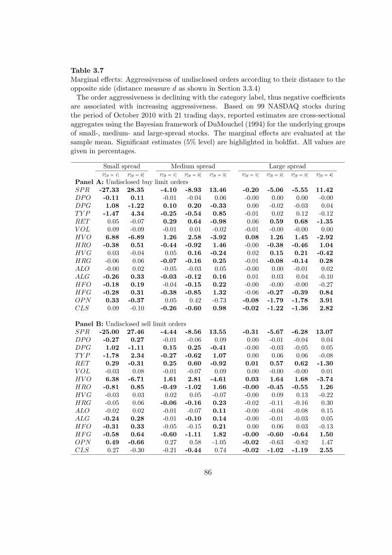
Table 3.7Marginal effects: Aggressiveness of undisclosed orders according to their distance to theopposite side (distance measure d as shown in Section 3.3.4)The order aggressiveness is declining with the category label, thus negative coefficients
are associated with increasing aggressiveness. Based on 99 NASDAQ stocks duringthe period of October 2010 with 21 trading days, reported estimates are cross-sectionalaggregates using the Bayesian framework of DuMouchel (1994) for the underlying groupsof small-, medium- and large-spread stocks. The marginal effects are evaluated at thesample mean. Significant estimates (5% level) are highlighted in boldfat. All values aregiven in percentages.
Small spread Medium spread Large spreadP[y = 1] P[y = 2] P[y = 1] P[y = 2] P[y = 3] P[y = 1] P[y = 2] P[y = 3] P[y = 4]
Panel A: Undisclosed buy limit ordersSPR -27.33 28.35 -4.10 -8.93 13.46 -0.20 -5.06 -5.55 11.42DPO -0.11 0.11 -0.01 -0.04 0.06 -0.00 0.00 0.00 -0.00DPG 1.08 -1.22 0.10 0.20 -0.33 0.00 -0.02 -0.03 0.04TY P -1.47 4.34 -0.25 -0.54 0.85 -0.01 0.02 0.12 -0.12RET 0.05 -0.07 0.29 0.64 -0.98 0.06 0.59 0.68 -1.35V OL 0.09 -0.09 -0.01 0.01 -0.02 -0.01 -0.00 -0.00 0.00HV O 6.88 -6.89 1.26 2.58 -3.92 0.08 1.26 1.45 -2.92HRO -0.38 0.51 -0.44 -0.92 1.46 -0.00 -0.38 -0.46 1.04HVG 0.03 -0.04 0.05 0.16 -0.24 0.02 0.15 0.21 -0.42HRG -0.06 0.06 -0.07 -0.16 0.25 -0.01 -0.08 -0.14 0.28ALO -0.00 0.02 -0.05 -0.03 0.05 -0.00 0.00 -0.01 0.02ALG -0.26 0.33 -0.03 -0.12 0.16 0.01 0.03 0.04 -0.10HFO -0.18 0.19 -0.04 -0.15 0.22 -0.00 -0.00 -0.00 -0.27HFG -0.28 0.31 -0.38 -0.85 1.32 -0.06 -0.27 -0.39 0.84OPN 0.33 -0.37 0.05 0.42 -0.73 -0.08 -1.79 -1.78 3.91CLS 0.09 -0.10 -0.26 -0.60 0.98 -0.02 -1.22 -1.36 2.82
Panel B: Undisclosed sell limit ordersSPR -25.00 27.46 -4.44 -8.56 13.55 -0.31 -5.67 -6.28 13.07DPO -0.27 0.27 -0.01 -0.06 0.09 0.00 -0.01 -0.04 0.04DPG 1.02 -1.11 0.15 0.25 -0.41 -0.00 -0.03 -0.05 0.05TY P -1.78 2.34 -0.27 -0.62 1.07 0.00 0.06 0.06 -0.08RET 0.29 -0.31 0.25 0.60 -0.92 0.01 0.57 0.62 -1.30V OL -0.03 0.08 -0.01 -0.07 0.09 0.00 -0.00 -0.00 0.01HV O 6.38 -6.71 1.61 2.81 -4.61 0.03 1.64 1.68 -3.74HRO -0.81 0.85 -0.49 -1.02 1.66 -0.00 -0.45 -0.55 1.26HVG -0.03 0.03 0.02 0.05 -0.07 -0.00 0.09 0.13 -0.22HRG -0.05 0.06 -0.06 -0.16 0.23 -0.02 -0.11 -0.16 0.30ALO -0.02 0.02 -0.01 -0.07 0.11 -0.00 -0.04 -0.08 0.15ALG -0.24 0.28 -0.01 -0.10 0.14 -0.00 -0.01 -0.03 0.05HFO -0.31 0.33 -0.05 -0.15 0.21 0.00 0.06 0.03 -0.13HFG -0.58 0.64 -0.60 -1.11 1.82 -0.00 -0.60 -0.64 1.50OPN 0.49 -0.66 0.27 0.58 -1.05 -0.02 -0.63 -0.82 1.47CLS 0.27 -0.30 -0.21 -0.44 0.74 -0.02 -1.02 -1.19 2.55
86

with the hidden order distance to the own side shown in Table 3.6 indicate that theeffect is negative for small-spread stocks but is positive for large-spread stocks.4 In par-ticular, for small spread stocks, one standard deviation increase of the spread impliesa decrease of the probability of hidden depth inside of the spread (category y = 1) byapproximately 6.7%. This finding supports the notion of liquidity-induced order place-ment which tends to be reduced if the spread widens and thus uncertainty rises (Hy-pothesis (1.A)). However, we find converse evidence for large-spread stocks where theprobability of hidden depth inside of the spread increases by approximately 7.3% if thespread widens by one standard deviation. This in line with Hypothesis (1.B) suggestingthat hidden order placements in (wider) spreads tends to be rather information-driventhan liquidity-driven.
Hence, we show that hidden order strategies tend to be different in low-spread stockscompared to those in large-spread stocks. This might be explained by different motiva-tions and types of market participants driving trading in small-spread vs. large-spreadstocks. In particular, we conclude from our findings that liquidity traders are morelikely to use aggressive hidden orders in small-spread stocks, but informed traders inhigh-spread stocks. We explain this by two reasonings. Firstly, small-spread stocks aregenerally more liquid. This makes it harder to hold informational advantage over a longertime period. Consequently, informed traders prefer visible orders or reserve orders whichhave time priority compared to hidden orders. In large-spread stocks, however, thereis more room to exploit and camouflage informational advantage which make hiddenorders more attractive than visible orders. Secondly, in small-spread stocks, the grid ofavailable tick points available for improving the quote is typically too limited. Therefore,even the most passive hidden order inside of the spread can be still too aggressive for aninformed traders.
Measuring the aggressiveness of hidden depth in terms of the distance to the oppositeside of the market (measure d), we find an overall negative effect. Hence, as shown bythe estimates in Tables 3.5 and 3.7, an undisclosed order is placed further away fromthe opposite side when the spread widens. This effect is consistent with the findings forsmall-spread stocks based on measure s, but it seems to be a contradiction of the resultsfor large-spread stocks. However, as the categorizations of the two distance measures arepartially overlapping, this seeming contradiction is explained by an increasing clusteringof aggressive hidden orders in regions close to the own side. The underlying mechanismis graphically illustrated in Figure 3.7 showing how the hidden depth concentrates moresignificantly on the own side if the spread widens. Intuitively, (informed) traders usehidden orders to compete for the provision of liquidity with own-side liquidity suppli-ers (and thus increase execution probabilities) while still balancing picking-off risks byremaining sufficiently “passive”. As a consequence of symmetric effects for sell orders,we can conclude that the “hidden” spread is positively correlated with the observablespread.
4As the estimates reported in Table 3.5 are aggregates across all stocks, they turn out to beinsignificant.
87

Figure 3.7: Stylized illustration of the effect of a widening of bid-ask spreads on hiddenorder placements for large-spread stocks. Left: scenario of a narrow spread; right:scenario of a wide spread. This illustration shows the effect of an increasing hiddenorder aggressiveness in terms of the distance to the own-side quote, coming along witha decreasing hidden order aggressiveness in terms of the distance to the opposite-sidequote.
3.5.2 (How) Does Hidden Liquidity Compete with VisibleLiquidity Provision?
Analyzing the effects of visible on-side depth on the best quotes (DPO), we find a clearconfirmation of Hypothesis (2.A). Hence, the probability of hidden depth inside of thespread is positively related to the own side visible depth. Table 3.6 reports that theprobability of using aggressive hidden bid limit orders increases by approximately 5.5%(2.3%) as the visible depth at the best bid increases by one standard deviation. Hence,traders increase the aggressiveness of hidden orders in order to compete for the provisionof liquidity and thus to increase execution probabilities. We again observe contradictingeffects for the two underlying distance measures in the case of small-spread stocks leadingto the same effects as illustrated in Figure 3.7. Hence, in case of small-spread stocksoffering not much room for (hidden) quote improvements, a higher (visible) own-sidedepth leads to a stronger clustering of hidden orders close to the own-side quote.
While Hypothesis (2.A) is clearly confirmed, we do not find supporting evidence forHypothesis (2.B). Indeed, Table 3.6 reports that the distribution of hidden depth tendsto move to the own side as the visible depth on the opposite side (DPG) increases inlarge-spread stocks, while no significant change takes place in small-spread stocks. Thisevidence is in line with the notion that hidden liquidity suppliers tend to reduce adverseselection risk if the price pressure on the opposite side becomes too high. This effectobviously overcompensates traders’ motivation to increase execution risk by becomingmore aggressive.
Measuring the aggressiveness of hidden depth in terms of the distance to the opposite-
88

Figure 3.8: Stylized illustration of the effect of an increase of visible ask depth onundisclosed buy order placements for medium-spread stocks. Left: scenario of a lessvisible depth ; right: scenario of a huge visible depth. This illustration shows the effectof an increasing hidden order aggressiveness in terms of the distance to the opposite-sidequote, coming along with no significant effects on the hidden order aggressiveness interms of the distance to the own-side quote.
Figure 3.9: Stylized illustration of the effect of an increase of visible ask depth onundisclosed buy order placements for large-spread stocks. Left: scenario of a less visibledepth ; right: scenario of a huge visible depth. This illustration shows the effect ofan decreasing hidden order aggressiveness in terms of the distance to the opposite-sidequote, coming along with no significant effects on the hidden order aggressiveness interms of the distance to the opposite-side quote.
89

side quote (measure d), we find positive effects in small- and medium-spread stocks. Asshown by the estimates in Tables 3.5 and 3.7, an undisclosed order is placed closer tothe opposite side when the opposite side visible depth increases. The seeming contradic-tion to estimates in Table 3.6 implying no significant effects could be explained by theincreasing use of reserve orders and the partially overlapping categories. We graphicallyillustrate the underlying mechanism in Figure 3.8 showing how traders update the own-side quote by the reserve order. A similar explanation can be reasoned for the seemingcontradiction of estimates in large-spread stocks as well (Figure 3.9). The finding sup-ports Buti and Rindi (2011)’s theoretical prediction that the use of reserve orders, ratherthan hidden orders, increases with the opposite-side visible depth. Pardo Tornero andPascual (2007) and De Winne and D’Hondt (2007) find similar evidence for the SpanishStock Exchange and Euronext Paris where only reserve orders but not hidden orderscan be used.
3.5.3 Hidden Order Placements After Price Movementsand Trading Signals
We show that the aggressiveness of hidden bid depth decreases when the prevailingtrade is seller-initiated (TYP). In particular, the hidden bid depth shifts away from theask side. This reduces liquidity suppliers’ risk of being picked off by (eventually betterinformed) sellers but increases their risk of non-execution. Conversely, in case of a buymarket order, hidden liquidity supply on the bid side increases and moves toward the askside. Hence, liquidity suppliers follow trading directions in the sense that they post moreaggressively and thus increase execution probabilities without facing too high adverseselection risk (as long as buy pressure dominates).
In this sense, Hypothesis (3.A) is confirmed. Besides economic reasoning, a puremechanical effect may further drive the results. In particular, as a sell trade itselfabsorbs pending aggressive undisclosed buy limit orders, the aggressiveness of hiddenbid depth temporarily decreases. This effect, however, is only true in case of tradesarriving instantaneously before the observation of interest. But as our estimates utilizeall order messages revealing information on hidden orders (occurring on average 30 timesmore frequently than trades), these mechanical effects apply only infrequently.
Analyzing the effects of recent price movements (RET ) on hidden order placements,we find similar effects and supportive evidence in favor of Hypothesis (3.B). Accordingly,the aggressiveness of undisclosed bid orders increases as prices have been moved upwards.Specifically, the probability of hidden orders inside of the spread increases approximately2.9% when the return increases by one standard deviation. Moreover, the estimates inTable 3.5 show that hidden bid depth moves closer to the ask side. Again, this supportsliquidity suppliers’ motivation to reduce the risk of non-execution. Conversely, in case ofprevailing negative price movements, hidden liquidity placements on the bid side becomeless aggressive with the hidden depth distribution shifting away from the ask side. Aspostulated in Section 3.2.3, this is explained by protection against picking-off risks incase prices continue moving downwards.
90

Interestingly, no clear confirmation of Hypothesis (4) is found. We do not findsignificant impacts of prevailing return volatility. According to our estimates, hiddenorder aggressiveness even tends to increase in volatile market periods. However, in mostcases, these effects are insignificant.
3.5.4 Competition for Hidden Liquidity Provision
Our estimates show clear evidence for hidden liquidity competition. According to theestimates associated with the effects of own-side hidden liquidity supply (HV O), wesupport Hypothesis (5). In particular, Table 3.6 reports that the probability of hiddenbid depth inside of the spread increases by approximately 10% as the execution of hiddenbid volume during the last minute increases by one standard deviation. This effect issupported by the estimates in Table 3.7 indicating that hidden liquidity shifts closer tothe opposite side of the market. Hence, according to the reasoning motivating Hypothe-sis (5), liquidity suppliers provide further hidden volume if they realize liquidity demandfrom the opposite side and competition on their own side.
Our estimates show that these effects prevail as long as adverse selection risk doesnot become too high. Indeed, when the prevailing one minute hidden depth executionbecomes too high compared to the corresponding activities during the last five minutes(HRO), hidden order aggressiveness tends to decline. In this situation, price pressurefrom the opposite side becomes too strong and makes adverse selection risk too high.
Studying the effect of hidden order detections on the opposite side of the market, wefind slight evidence for the effect that trading against hidden sell orders also increasesthe hidden order aggressiveness on the bid side. This might be explained by the factthat buy market orders make buy hidden orders (relatively) less aggressive and moveaway hidden ask quotes. This, in turn, gives hidden liquidity suppliers on the bid sidemore room for quote improvements and thus the reduction of non-execution risks.
3.5.5 Hidden Order Placements and HFT
Analyzing the effects of HFT (approximated by the intensity of fleeting orders) on hiddenorder submissions, we find strong empirical support for Hypothesis (6). Indeed, the moreopposite-side traders try to detect hidden liquidity by “pinging activities” (HFG), thelower the hidden order aggressiveness. Especially for large-spread stocks, an one standarddeviation increase of HFT activities on the ask side implies a decrease of the probabilityof hidden bid depth placements inside of the spread by more than 5%. Consequently,the distribution of hidden depth moves away from the opposite quote. Hence, tradersinterpret the rapid cancellations of limit orders as signals for hidden liquidity detectionstrategies rather than true liquidity supply. These results are in line with empiricalevidence reported by Hasbrouck and Saar (2009) and the predictions by Buti and Rindi(2011) showing that hidden order placements become non-attractive if hidden depth iseasily detected.
Note that the effects on the distribution of the entire hidden depth (as reported in
91

Table 3.7) are substantially smaller than those on hidden depth inside of the spread (asrevealed by Table 3.6). This finding also supports the theoretical prediction by Buti andRindi (2011) that reserve orders, rather than hidden orders, are dominantly used whenparasitic traders utilize front running strategies.
3.5.6 Intraday Patterns
We find no clear confirmation of Hypothesis (7.A) postulating a higher hidden orderaggressiveness during or after the opening period. Actually, our findings for small-spreadstocks support the hypothesis, while it is rejected for large-spread stocks. However, clearevidence for Hypothesis (7.B) is shown. Indeed, for large-spread stocks, we find thatthe probability for hidden bid depth placements within the spread in the hour beforemarket closure is approximately 5% lower than during the rest of the day. This supportsthe economic reasoning that displayed orders are preferred if the time horizon becomesshorter and the importance of time priority rises.
3.6 Conclusion
Many stock exchanges around the world choose to reduce market transparency by al-lowing traders to hide a portion of their order size. As a consequence trading underlimited pre-trade transparency becomes increasingly popular in financial markets. Pre-vious studies in the literature examine opaque markets with only partially undisclosedorders. This study sheds light on traders’ use of completely undisclosed orders in elec-tronic trading, based on a sample of 99 stocks traded on NASDAQ during October2010.
Employing NASDAQ TotalView message data, we retrieve information on hiddendepths from the visible order activities and propose an ordered response approach withcensoring mechanism for modelling the hidden order locations conditional on the state ofmarket. Our finding shows that the hidden liquidity supply has significantly correlationto the market conditions and thus is predictable in terms of the state of the prevailing(visible) LOB and order flow. The evidence suggests that traders make their undisclosedorder submission strategies by balancing the non-execution risk and picking-off risk.
Our findings are of interest to academics and institutional trading desks. A betterunderstanding of traders’ decisions on using undisclosed orders could help theorists indeveloping comprehensive models on trader behaviour in opaque markets with both hid-den order types. Moreover, these results provide useful insights for institutional traderswho are obligated to acquire a big position. They may benefit by either improving theirundisclosed order submission strategies or searching for hidden depths on the oppositeside of the market more efficiently.
92

Chapter 4
Extracting Information from theMessage Stream
This chapter is based on Huang and Polak (2011).
4.1 Introduction
An electronic limit order market is an order-driven market which automatically collectsorders from traders in a centralized limit order book (LOB) and matches correspondingbuy and sell orders based on specific priority rules, very often the price-time priorityrule. Currently, most equity exchanges around the world are either pure electronic limitorder markets, e.g. NYSE Arca, BATS, Euronext, Australian Stock Exchange (ASX) andDirect Edge, or at least allow for customer limit orders in addition to on-exchange marketmaking, e.g. NASDAQ, NYSE and the London Stock Exchange (LSE). The traditionalmonopolistic power of market makers in the area of liquidity provision through quotingon both sides of the market has been strongly restricted, if not completely eliminated.Instead, the important task of providing liquidity is now assigned to the complex tradinginteractions enabled by the emergence and disclosure of the LOB. Hence, the state ofthe LOB is extremely important for practitioners, because it allows them to optimizetheir trading strategies, but also for researchers who analyze trading activity in thesemarkets and try to interpret the underlying economic motivation.
One of the most prominent market structure developments in recent years is highfrequency (“HF”) trading. HF traders in general employ extremely quick and sophisti-cated computer programs for generating, routing and executing orders. They establishand liquidate positions in very short time-frames by submitting numerous orders andcancelling non-executed orders shortly after submission. As a consequence, the tradingvolume grows, orders shrink in size and the pace of LOB updating is beyond humanperception, requiring nanosecond precisions. The volume of information about ordersrecorded by market organizers therefore dramatically increases.
More than ever before researchers today face the challenge of working with real
93

datasets on micro-structure level of financial markets. They are in general not difficultto obtain, but very difficult to process. One way of going about it is acquiring snapshotsof historical LOB data. But this is very impractical, because such datasets are usuallyvery large and contain only incomplete information1. The second option is to acquiremuch better compressed raw message stream data, like TotalView-ITCH and MulticastPITCH data. Because message data record all visible order activities, i.e. limit ordersubmissions, cancellations and executions, they can be used to reconstruct the historicalLOB up to any required precision (level). However, this creates a different type ofchallenge; it is necessary to reconstruct the LOB using the same rules that were usedby the matching algorithm applied by the exchange. Although simple in principle, suchalgorithms need to take into account market-specific issues and, considering the largevolume of data, work extremely efficiently.
In this chapter, we present you the LOBSTER, a program framework for reconstruct-ing LOBs as well as extracting order flow information from historical message streamdata. Note that the fundamental limit order activities are quite similar across differentlimit order markets, though the specific trading rules can be very different. We mod-ularize LOBSTER to processes limit order activities translated from messages insteadof messages themselves, so that it can be easily adapted to data from new limit ordermarkets with just a few modifications. The underlying data structure in these modules ishighly optimized and their programs are exhaustively tested to guarantee the reliabilityof the output data and the efficiency of the entire system.
Currently we implement a translation module for NASDAQ TotalView-ITCH mes-sage and a web-based interface. Researchers around the world can easily access ourprogram through http://lobster.wiwi.hu-berlin.de and download NASDAQ LOBdata reconstructed on the fly. Moreover, a related forum facilitates general discussionon empirical analysis of LOB, as well as bundles of small programs and useful tools inboth R and Matlab.
The remainder of this chapter is structured as follows. In Section 4.2, we take theNASDAQ TotalView-ITCH as an example to illustrate the structure of order-relatedmessages in message stream data. Section 4.3 gives the overview of the design of theLOBSTER. We discuss in detail on two implemented modules, the LOB Constructor andthe Order Tracer, in Section 4.4 and 4.5, respectively. Finally, Section 4.6 concludes.
4.2 Message Stream Data
As we already discussed above, unlike historical snapshots of the LOB, message-type dataallow reconstructing the full LOB and observing its dynamics with maximum precision.This is indeed extremely valuable for academic research, giving the possibility to studyall aspects of trading in full detail. In this section, we will take the NASDAQ TotalView-
1Snapshots are made at regular time intervals, e.g. every second, which means that multiplechanges within this time intervals may be omitted. Should snapshots capture all changes in theLOB to all levels the size of files to store these datasets would be too large for practical purposes.
94

Table 4.1TotalView-ITCH: order-related messages.TotalView-ITCH includes messages representing submissions, executions and cancel-
lations of limit orders, as well as executions of hidden orders. A submission type limitorder message may or may not contain information identifying the market participant,who submitted the order - Market Participant Identification (MPID). A type “P” mes-sage reports the execution price and immediately traded quantity, i.e. only that part ofthe hidden order, which is currently being executed against an incoming order. Thus noinformation about the remaining unexecuted part of the hidden order is revealed.
Instruction Type Limit/Hidden Order Canc./Exe.ID Price Size MPID size
Limit order submission A X X X
Limit order submission with MPID F X X X X
Limit order execution E X X
Limit order cancellation (partially) X X X
Limit order cancellation (totally) D X
Hidden order execution P X X X
ITCH 4.0 as an example to illustrate the structure of messages.The original NASDAQ TotalView-ITCH is a direct data feed that contains market
messages for all submissions, cancellations and executions of limit orders, as well asexecutions of hidden orders. TotalView-ITCH 4.0 data is the binary version of theTotalView-ITCH data introduced in November 2008, following the ITCH 3.0 format.This format is ready for nanosecond time stamps2 and contains longer order and tradeidentification numbers allowing to mark up to 18 quadrillion messages per day.
Considering the enormous number of messages generated by the activities in mar-kets every day, the TotalView message stream is designed to present information in aparsimonious way, reducing redundancy in the records. Table 4.1 illustrates the mes-sage types related to the instructions carried by orders. Whenever a market participantsubmits a new order, its details, such as order ID, limit price and size, are recorded ina submission message. If the market participant chooses to reveal her identity to othermarket participants the submission message contains also her Market Participant Iden-tification (MPID). All subsequent changes to the submitted limit order are also recordedin the form of messages; messages reporting partial cancellations or executions (partialor total) contain the same order ID as the original submission messages and the cancelledor executed quantity. If the limit order is totally cancelled (deleted), TotalView recordsonly the corresponding order ID. Finally, messages reporting executions of hidden orderscontain only the price and the executed quantity, but not the total size of the originallysubmitted hidden orders.
2The time resolution of trading in NASDAQ is still in milliseconds. Therefore, the timestamps in the current data set have still millisecond precision rather than nanosecond.
95
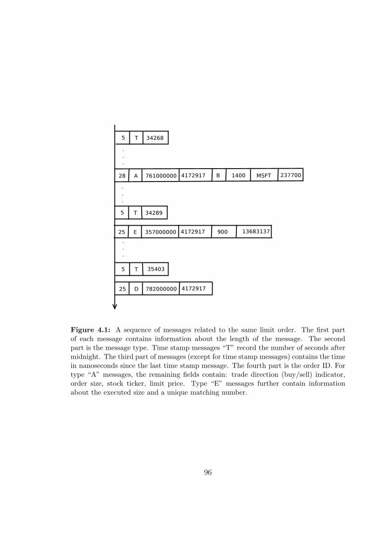
Figure 4.1: A sequence of messages related to the same limit order. The first partof each message contains information about the length of the message. The secondpart is the message type. Time stamp messages “T” record the number of seconds aftermidnight. The third part of messages (except for time stamp messages) contains the timein nanoseconds since the last time stamp message. The fourth part is the order ID. Fortype “A” messages, the remaining fields contain: trade direction (buy/sell) indicator,order size, stock ticker, limit price. Type “E” messages further contain informationabout the executed size and a unique matching number.
96
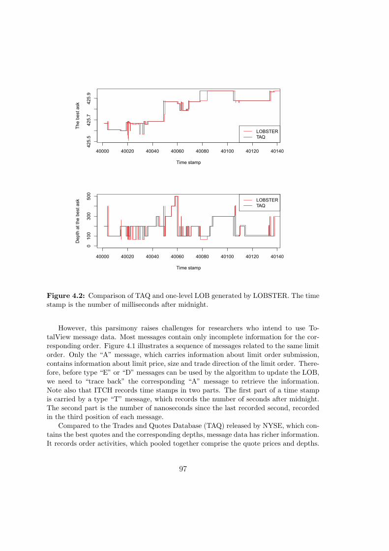
40000 40020 40040 40060 40080 40100 40120 40140
425.
542
5.7
425.
9
Time stamp
The
best
ask
LOBSTERTAQ
40000 40020 40040 40060 40080 40100 40120 40140
010
030
050
0
Time stamp
Dep
th a
t the
bes
t ask LOBSTER
TAQ
Figure 4.2: Comparison of TAQ and one-level LOB generated by LOBSTER. The timestamp is the number of milliseconds after midnight.
However, this parsimony raises challenges for researchers who intend to use To-talView message data. Most messages contain only incomplete information for the cor-responding order. Figure 4.1 illustrates a sequence of messages related to the same limitorder. Only the “A” message, which carries information about limit order submission,contains information about limit price, size and trade direction of the limit order. There-fore, before type “E” or “D” messages can be used by the algorithm to update the LOB,we need to “trace back” the corresponding “A” message to retrieve the information.Note also that ITCH records time stamps in two parts. The first part of a time stampis carried by a type “T” message, which records the number of seconds after midnight.The second part is the number of nanoseconds since the last recorded second, recordedin the third position of each message.
Compared to the Trades and Quotes Database (TAQ) released by NYSE, which con-tains the best quotes and the corresponding depths, message data has richer information.It records order activities, which pooled together comprise the quote prices and depths.
97

Figure 4.3: The overview of LOBSTER system. Three types of modules are used ingeneral. Readers (green) read the source data into the system; data Processors (purple)retrieve the information; Writers (blue) write the output into the file system. For thesake of flexibility Readers and Writers are normally implemented as interfaces.
Thanks to this superiority of information content message data can be used to recon-struct the LOB up to any quote level. But even when looking only at the best quoteand depth, message data is richer than the usual data obtained from the TAQ database.Message data contain information about limit orders which are cancelled shortly afterthe submission. These limit orders are typically submitted in order to detect hidden liq-uidity inside the spread rather than to provide liquidity (see e.g., Hasbrouck and Saar,2009). Therefore, it is not surprising that TAQ ignores them as shown in Figure 4.2.However, these orders are crucial for some studies, e.g the analysis of high frequencytrading strategies and hidden order submission strategies.
The currently implemented LOBSTER is connected to a storage facility containingover 5 TB of historical TotalView-ITCH data, in ITCH 3.0 format from the period Jan2007 to Apr 2009 and ITCH 4.0 format from the period May 2009 to Dec 2010. Thisdataset contains only limit order messages. Other messages such as imbalance dataevents and administrative messages have been cleaned out.
4.3 Overview of LOBSTER
The main goal of LOBSTER is to provide a reliable, efficient and flexible platform forresearchers to retrieve information from parsimonious message data. Relying on theobject-oriented concept, we designed LOBSTER as a modular system with three typesof modules: Readers(green), data Processors(purple) and Writers(blue) as shown inFigure 4.3.
Reader translates data from an external source to a stream of order events, which is
98

then processed by data Processors. Based on a unified abstract interface, differentreaders can be created for reading different input formats, e.g. from different stockexchanges. But also an order-flow simulator can act as a “Reader”, provided thatthe generated data have the required format. Currently the system contains anITCH message Reader for reading binary ITCH files from the storage facility anda test version PITCH Reader for BATS.
Data Processor is the core of the system responsible for extracting the informationrequired by users from the order flow generated by Reader. Connected to Readerby an abstract interface, the data Processors treat historical order flow, simulatedorder flow or hybrid order flow identically. This creates great potential for veryeffective testing of trading strategies.3
We implemented a LOB Constructor that matches the limit orders coming fromthe Reader and updates the LOB. The accuracy and efficiency of this algorithmdetermine to a large extent the overall performance of the system. For this reason itwas thoroughly tested and optimized. We shall discuss the currently implementedLOB Constructor in Section 4.4.
Moreover, we have also developed Order Tracer, whose beta version is currentlybeing tested. Order Tracer traces relevant events for individual limit orders, suchas the time of submission, partial/full execution and cancellation. It has been usedfor computing the lifetime of limit orders for some research projects (e.g. Hautschand Huang, 2012a,c). We expect that in the near future more and more utilitiesfor special research purposes will be added to the current framework.
Writer receives the reconstructed data and saves them to the file system. Currentlythe system contains four Writers; the Message Writer, which saves the event typeand the corresponding order information into the file system, the Book Writer,which receives the current state of the reconstructed LOB for every order eventand saves it, the Order Writer, which saves the characteristics (order ID, limitprice, size, etc.) of limit orders, and finally the Trace Writer, which saves event-specific information, such as the event time, submission time and the type of orderevent, as generated by the Order Tracer.
99
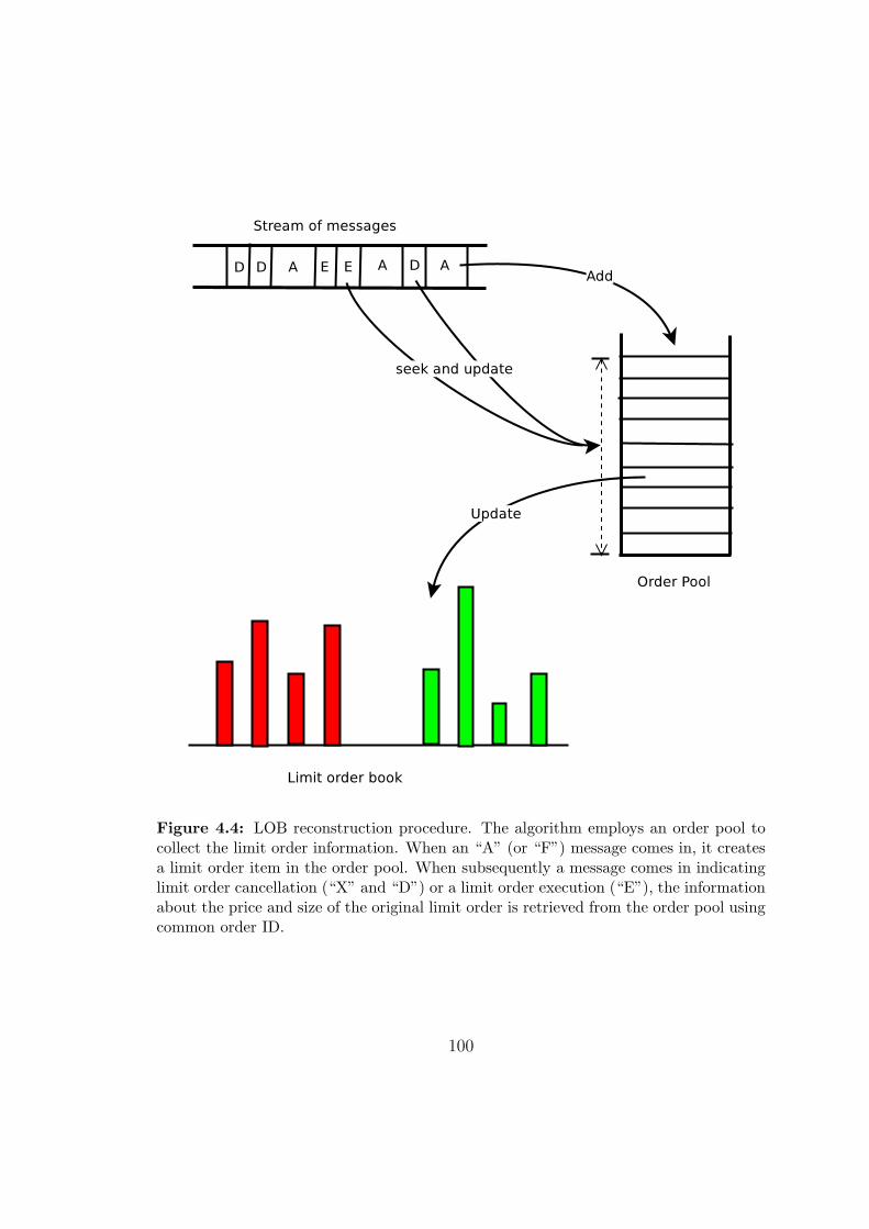
Figure 4.4: LOB reconstruction procedure. The algorithm employs an order pool tocollect the limit order information. When an “A” (or “F”) message comes in, it createsa limit order item in the order pool. When subsequently a message comes in indicatinglimit order cancellation (“X” and “D”) or a limit order execution (“E”), the informationabout the price and size of the original limit order is retrieved from the order pool usingcommon order ID.
100
4.4 Limit Order Book Reconstruction
4.4.1 Overview of the Reconstruction Procedure
Figure 4.4 summarizes the procedure of the LOB reconstruction. For arriving messagesidentified as limit order submissions, the system records in the order pool all relevantinformation including order ID, limit price, quantity, trade direction and MPID, if avail-able. Once a cancellation or execution message arrives, the system first finds in the poolthe corresponding previously recorded limit order submission by comparing the orderIDs. After matching the two orders - incoming order and order stored in the order pool- the system records the remaining non-executed size of the limit order or deletes theorder from the order pool altogether if the remaining size is zero. Finally, the systemupdates the LOB: the side in the LOB (bid or ask) to be updated is determined by tradedirection (buy or sell) of the corresponding order; the level in the LOB is identified bythe limit price; the new depth at this level is calculated by deducting the size of theeffective quantity.
The remaining issue is the construction of the initial-state of the LOB before theaforementioned procedure can be applied. Note that in the TotalView-ITCH messagedata, the order ID of any limit order cancellation and execution message can always befound in a limit order submission message, which was recorded at an earlier time on thesame trading day. This implies that all limit orders valid overnight, such as some good-to-kill orders, have been resubmitted by the system in the early morning. The NASDAQtrading system is in general open for new order instructions at 7:00 EST, even thoughcontinuous trading does not start until 9:30 EST. Because the TotalView-ITCH data setcontains all messages, including messages submitted during the pre-trading period, ouralgorithm initializes the reconstruction with an empty LOB at the beginning of everyday.
4.4.2 Implementation of LOB Constructor
As we discuss in Section 4.2, all TotalView-ITCH messages, except for messages con-taining limit order submissions, contain only partial information about the underlyinglimit orders. In order to update the order book, we need to “complete” the limit orderinformation. Figure 4.5 shows in details how this is done in case of messages containinglimit order executions. After reading an execution message, the system searches for thecorresponding limit order inside the order pool using the order ID. If the search is suc-cessful, the information on the remaining size of the limit order is updated. The systemthen updates the LOB by changing the depth and quote on the corresponding level.
3For instance, it is well-known that the back-testing of trading strategies on historical datahas a very serious drawback - there is no market feedback to the tested strategy and so it is veryhard to estimate the market impact of the strategy. In this context, testing with a simulatorallows implementing realistic feedback mechanisms to simulate market impact and thus providecredible assessment of the tested trading strategy.
101

Figure 4.5: Sequential diagram for messages of limit order executions. The procedure begins with reading the message andcreating a corresponding Message object. The object then communicates with the order pool and updates information aboutthe underlying limit order. Simultaneously, it retrieves from the limit order any missing information, such as price. Usingthe complete information about the limit order, the Message object updates the order book state (the OrderBook object).Finally, the constructor writes the updated order book state and the corresponding message into the file system using theOrderBookWriter and MessageWriter objects.
102

Figure 4.6: Class diagram of LOB construction. A BookConstructor object containsunique OrderBook and OrderPool objects, which are updated using incoming messagescorresponding to Message objects. Moreover, there must be at least one MessageReaderobject for reading the input, an OrderBookWriter object and a MessageWriter object,which write the output into the file system.
Finally, the new order book and the corresponding message item are stored in the filesystem as output.
Figure 4.6 represents the final class diagram for our LOB Constructor. The systemincludes a unique OrderBook and OrderPool instance, which are controlled via a uniqueBookConstructor instance. After MessageReader objects reads a message from anexternal source, it creates a Message object and then uses it to update the limit ordersinside the OrderPool object as well as quote and depth information in the OrderBook
object according to the order event type. If the process is successful, it saves the outputusing a MessageWriter and an OrderBookWriter object. Note that the Reader andWriter are intent to be defined as abstract interfaces, rather than concrete classes, forincreasing the flexibility of the format of output data.
4.4.3 Output of LOB Constructor
The LOB Constructor generates two output data files; one file contains the LOB dataand the other one contains the corresponding order events. Table 4.2 shows a segment of
103

Table 4.2LOB data generated by the LOB Constructor.The sample contains a five second segment of three-level LOB data for ticker GOOG on July 1st 2009. The time variable
is in milliseconds after the midnight. Price is in 0.01 of a cent and size in number of shares. The corresponding order eventsthat update the state of the LOB are shown in Table 4.3.
Time Ask Ask Bid Bid Ask Ask Bid Bid Ask Ask Bid Bidprice 1 size 1 price 1 size 1 price 2 size 2 price 2 size 2 price 3 size 3 price 3 size 3
36000043 4231100 100 4227300 300 4231200 100 4223000 100 4231300 300 4222900 10036000044 4231100 100 4227300 300 4231200 300 4223000 100 4231300 300 4222900 10036000207 4229100 100 4227300 300 4231100 100 4223000 100 4231200 300 4222900 10036000208 4229100 100 4227300 300 4231100 100 4223000 100 4231200 100 4222900 10036000208 4229100 100 4227300 300 4231100 100 4223000 100 4231300 100 4222900 10036003222 4229100 100 4227300 300 4231100 100 4223000 100 4231200 100 4222900 10036003471 4229100 100 4227300 300 4231100 100 4222900 100 4231200 100 4221200 10036004005 4229100 200 4227300 300 4231100 100 4222900 100 4231200 100 4221200 10036004009 4229100 200 4227300 200 4231100 100 4222900 100 4231200 100 4221200 10036004009 4229100 200 4222900 100 4231100 100 4221200 100 4231200 100 4219100 40036004009 4229100 200 4222900 100 4231100 100 4221200 100 4231200 100 4219100 40036004010 4229100 200 4222900 200 4231100 100 4221200 100 4231200 100 4219100 40036004010 4229100 200 4227300 200 4231100 100 4222900 200 4231200 100 4221200 10036004011 4229100 100 4227300 200 4231100 100 4222900 200 4231200 100 4221200 10036004015 4229100 100 4227300 200 4231100 100 4223300 100 4231200 100 4222900 20036004016 4229100 100 4227300 200 4231100 100 4222900 200 4231200 100 4221200 10036004017 4229100 100 4222900 200 4231100 100 4221200 100 4231200 100 4219100 40036004018 4229100 100 4222900 200 4231100 100 4222800 200 4231200 100 4221200 10036004018 4229100 200 4222900 200 4231100 100 4222800 200 4231200 100 4221200 10036004018 4229100 200 4227300 200 4231100 100 4222900 200 4231200 100 4222800 20036004020 4229100 200 4227300 200 4231100 100 4222900 200 4231200 100 4221200 10036004020 4229100 100 4227300 200 4231100 100 4222900 200 4231200 100 4221200 10036004021 4229100 100 4227300 200 4231100 100 4223300 100 4231200 100 4222900 20036004025 4229100 100 4223300 100 4231100 100 4222900 200 4231200 100 4221200 10036004025 4229100 100 4222900 200 4231100 100 4221200 100 4231200 100 4219100 400
104

Table 4.3Order event data generated by the LOB Constructor.The sample contains a five second segment of order event (affecting the three-level
LOB) data for ticker GOOG on July 1st 2009. The time variable is in milliseconds af-ter the midnight. The type variable indicates the event type: submission, cancellation,execution of a limit order or execution of a hidden orders. Order ID is the ID of thecorresponding limit or hidden order. Size is the effective size, i.e. order size for submis-sion events and cancelled (executed) quantity for cancellation (execution) events. Thethree-level LOB instances immediately after these order events are shown in Table 4.2.
Time Type Order ID Size Price Trade Direction
36000043 1 35859474 100 4231100 -136000044 1 35859503 200 4231200 -136000207 1 35862501 100 4229100 -136000208 3 35859503 200 4231200 -136000208 3 35603811 100 4231200 -136003222 1 35926475 100 4231200 -136003471 3 35293758 100 4223000 136004005 1 35948533 100 4229100 -136004009 4 35332615 100 4227300 136004009 4 35643198 200 4227300 136004009 5 35643169 200 4227300 136004010 1 35948820 100 4222900 136004010 1 35948851 200 4227300 136004011 3 35948533 100 4229100 -136004015 1 35949144 100 4223300 136004016 3 35949144 100 4223300 136004017 4 35948851 200 4227300 136004018 1 35949411 200 4222800 136004018 1 35949425 100 4229100 -136004018 1 35949469 200 4227300 136004020 3 35949411 200 4222800 136004020 3 35949425 100 4229100 -136004021 1 35949745 100 4223300 136004025 4 35949469 200 4227300 1
105

reconstructed three-level LOB data for Google Inc. (with ticker GOOG in NASDAQ). Itincludes quotes and the corresponding depths up to the third best ask and bid, togetherwith time stamps. The other file contains the corresponding order event. As shown inTable 4.3, it has five fields:
• time: time stamp; milliseconds after mid-night.
• type: event type; 1 for limit order submission, 2 for partial cancellation, 3 fortotal deletion, 4 for limit order execution, 5 for hidden order execution.
• order ID: a unique number assigned by the exchange for identification of orders.
• size: change of order size (in shares); for limit order submission it is the ordersize, for order execution it is the trading volume and for limit order cancellationit is the cancelled volume.
• price: the price of the limit order or the corresponding executed hidden order (in0.01 of a cent).
• trade direction: the trade direction of the corresponding limit (hidden) order;1 for buy limit order and −1 for sell limit order. Note that in case of orderexecution, 1 corresponds to seller-initiated trade (i.e. execution against buy limitorder) while −1 corresponds to buyer-initiated trade (i.e. execution against selllimit order).
Both files can be easily loaded and used by analytical software, such as Matlab andR. Because the number of output order events is identical to the number rows in theLOB (i.e. both files have the same number of rows), the two output files can be easilymerged. The following is an example of R code for loading and merging the data set.
An Example of R Code Loading LOB Data
######### load data ########################
# load order book data
dataOB <− read . csv ( ”GOOG 20090701 orderbook 3 . csv ” )# load message data
dataM <− read . csv ( ”GOOG 20090701 message 3 . csv ” )# merge two da ta s e t s
data <− cbind (dataM , dataOB [ , −1 ] )####### load completed ###################
# compute the number o f order book l e v e l s
n l e v e l s <− (dim(dataOB ) [ 2 ] − 1)/4# name the columns
colnms <− c ( ”Time” , ”Type” , ”OrderID” , ” S i z e ” , ” Pr i ce ” , ”TradeDirect ion ” )for ( i in 1 : n l e v e l s ) colnms <− c ( colnms , paste ( ”ASKp” , i , sep=”” ) , paste ( ”ASKv” , i , sep=”” ) ,
paste ( ”BIDp” , i , sep=”” ) , paste ( ”BIDv” , i , sep=”” ) ) colnames ( data ) <− colnms
106

# clean up
rm( ’dataOB ’ , ’dataM ’ )
4.4.4 Application: Visualization of LOB and Order Flow
The purpose of the LOB and order flow visualization is to help researchers intuitivelyunderstand the basic principles of order-driven trading by showing a sequence of changesin the LOB associated with the incoming order events. The upper left box in Figure 4.7contains basic information about the displayed ticker and current time, as well as acomment field, which interprets the situation at the given point in time, thus helping tounderstand the principles better. The box labeled “Order Flow” shows several ordersaround the current order (violet color), as recorded in the corresponding output file. Thebox Limit Order Book (Table) box contains rows from the LOB that correspond to theorders displayed in the Order Flow box. The Limit Order Book (Table) box containsprices and depth (number of shares) at three levels of bid and ask. The box with the title“Limit Order Book (Graph)” contains the same information (for one row) visualized;depth (number of shares) at the three levels of displayed order book. Note that thisgraph contains only the current state of the LOB corresponding to the violet row in theprevious two boxes. Finally, the large graph on the right displays the incoming ordersand the continuity of BID and ASK price levels against the time axis. Note that thisgraph does not contain information about the size of incoming orders nor the cumulateddepth. But in combination, both graphs contain all information from the tables and thusprovide current snapshots, as well as the dynamics of the LOB in the sample period.
4.5 Order Tracer
We also implement a module called Order Tracer to extract information, i.e. cancella-tion, execution and deletion, for single limit orders. The procedure is similar to the LOBConstructor.
4.5.1 Implementation of Order Tracer
Reusing the classes designed for the LOB Constructor, we implement another appli-cation by adding one additional controlling class - the TraceRecorder. It passes themessage data and completes information from the underlying limit orders exactly inthe same way as the LOB Constructor. However, rather than using the information toupdate the LOB, it simply records the types of events and limit orders temporarily in ablock of memory called tracePool. The constructed data are then saved by instancesof LimitOrderWriter and TraceWriter. Figure 4.8 contains our final class diagram.
107

The Order with type Hidden Execution and trade direction Sell at price 143.74$ has arrived.
Description
TICKER = APPLE, TIME = 10:00:50.036
Time10:00:50.03210:00:50.03610:00:50.03610:00:50.052
TypeSubmission
Visible ExecHidden Exec
Deletion
OrderID37315193372805823731512037315130
Size100 50 50100
Price143.78143.74143.74143.78
TradeSellBuyBuy
Sell
Order Flow
20 22 24 26 28
143.72
143.74
143.76
143.78
143.80
143.82
Tick time
Price
Hidden Execution Visible ExecutionNew Submission Deletion
Snapshot of Order flow and LOB at 10:00:50.036 for 3 levels
BLevel 3143.72(600)
143.71(1100)143.71(1100)143.71(1100)
BLevel 2143.73(200)143.72(600)143.72(600)143.72(600)
BLevel 1143.74(50)
143.73(200)143.73(200)143.73(200)
ALevel 1143.78(400)143.78(400)143.78(400)143.78(300)
ALevel 2143.79(153)143.79(153)143.79(153)143.79(153)
ALevel 3143.8(1800)143.8(1800)143.8(1800)143.8(1800)
Limit Order Book (Table)
BID PRICE(BID SIZE) ASK PRICE(ASK SIZE)
143.72 143.74 143.76 143.78 143.80
500
1000
1500
Price($)
Volume
Limit Order Book (Graph)
BID ASK
Figure 4.7: The visualization of LOB and order flow. The time X-axis in the right graph does not correspond to the realtime, but rather to “tick time”, i.e. events in this graph are equidistant with respect to the X-axis regardless of their actualdistance in time. The Y-axis “Price” is scaled realistically to represent the actual quotes in the LOB. The current orderevent and LOB instance are highlighted by violet color in the left graph and by orange color in the right graph.
108

Figure 4.8: Class diagram of trace construction. A TraceRecorder object containsunique OrderPool objects, which are updated by incoming messages corresponding tothe Message objects. Also, it must include at least one MessageReader object for readingthe input, a LimitOrderWriter object and a TraceWriter objects for writing the outputinto the file system.
4.5.2 Output of Order Tracer
Similar to the LOB Constructor, the Order Tracer generates two files with the samenumber of rows. The first output file classifies events as cancellations or executions andcontains the following six columns (see a sample in Table 4.4).
• submission time: the time when the corresponding limit order was submitted;milliseconds after midnight.
• time: time stamp of the event; milliseconds after midnight.
• size: change of limit order size; number of shares.
• execution: a dummy variable indicating whether the event corresponds to a limitorder execution (1) or cancellation (0).
• earlier exe.: a dummy variable indicating whether the event corresponds to alimit order that has been partially executed earlier (1) or not (0).
The second output file contains information about the corresponding limit orders.Table 4.5 contains a segment of this file. There are seven variables:
• order ID: a unique number generated by the exchange identifying the limit order.
109
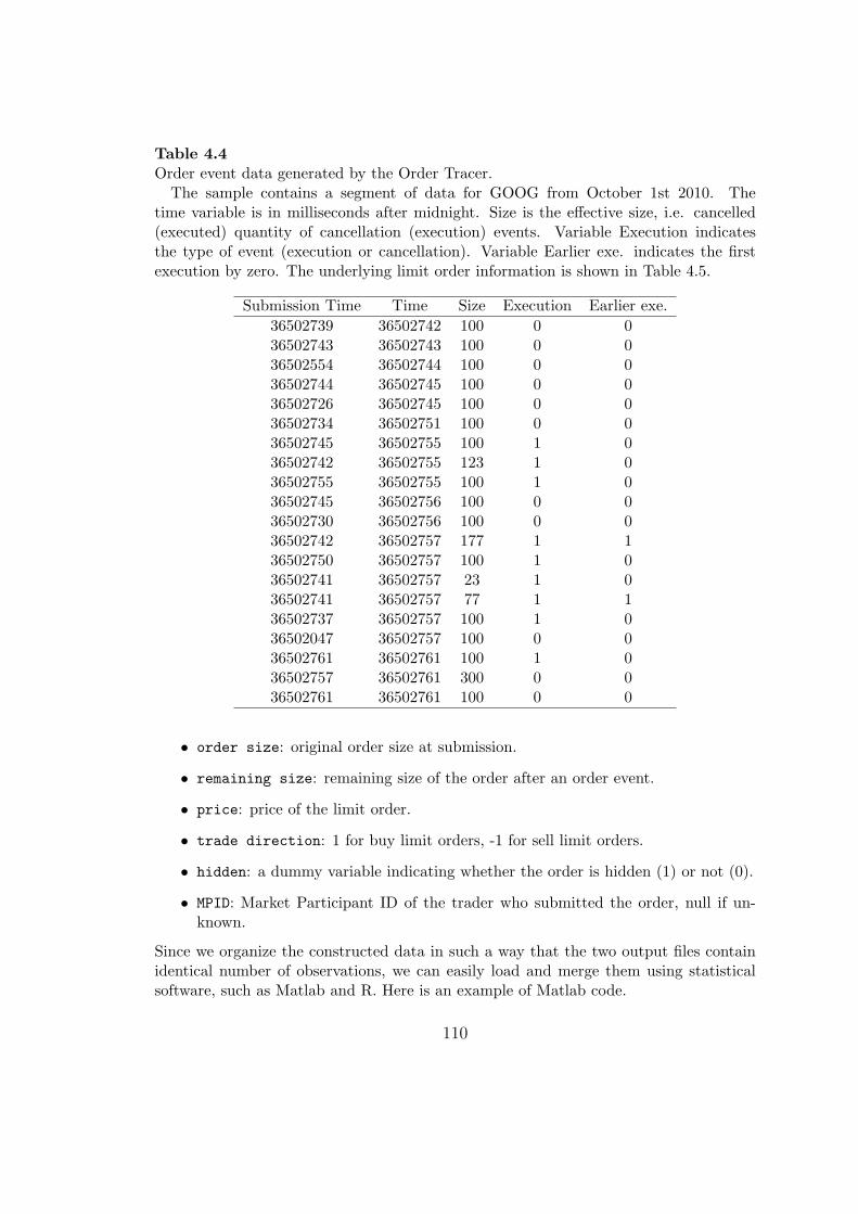
Table 4.4Order event data generated by the Order Tracer.
The sample contains a segment of data for GOOG from October 1st 2010. Thetime variable is in milliseconds after midnight. Size is the effective size, i.e. cancelled(executed) quantity of cancellation (execution) events. Variable Execution indicatesthe type of event (execution or cancellation). Variable Earlier exe. indicates the firstexecution by zero. The underlying limit order information is shown in Table 4.5.
Submission Time Time Size Execution Earlier exe.
36502739 36502742 100 0 036502743 36502743 100 0 036502554 36502744 100 0 036502744 36502745 100 0 036502726 36502745 100 0 036502734 36502751 100 0 036502745 36502755 100 1 036502742 36502755 123 1 036502755 36502755 100 1 036502745 36502756 100 0 036502730 36502756 100 0 036502742 36502757 177 1 136502750 36502757 100 1 036502741 36502757 23 1 036502741 36502757 77 1 136502737 36502757 100 1 036502047 36502757 100 0 036502761 36502761 100 1 036502757 36502761 300 0 036502761 36502761 100 0 0
• order size: original order size at submission.
• remaining size: remaining size of the order after an order event.
• price: price of the limit order.
• trade direction: 1 for buy limit orders, -1 for sell limit orders.
• hidden: a dummy variable indicating whether the order is hidden (1) or not (0).
• MPID: Market Participant ID of the trader who submitted the order, null if un-known.
Since we organize the constructed data in such a way that the two output files containidentical number of observations, we can easily load and merge them using statisticalsoftware, such as Matlab and R. Here is an example of Matlab code.
110
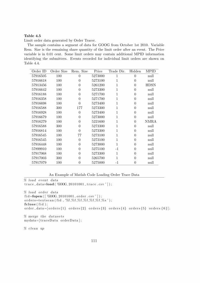
Table 4.5Limit order data generated by Order Tracer.The sample contains a segment of data for GOOG from October 1st 2010. Variable
Rem. Size is the remaining share quantity of the limit order after an event. The Pricevariable is in 0.01 cent. Some limit orders may contain additional MPID informationidentifying the submitters. Events recorded for individual limit orders are shown onTable 4.4.
Order ID Order Size Rem. Size Price Trade Dir. Hidden MPID
57916505 100 0 5273000 1 0 null57916618 100 0 5273100 1 0 null57913456 100 0 5261200 1 0 HDSN57916642 100 0 5273300 1 0 null57916188 100 0 5271700 1 0 null57916358 100 0 5271700 1 0 null57916698 100 0 5273400 1 0 null57916588 300 177 5273300 1 0 null57916928 100 0 5273400 1 0 null57916679 100 0 5273000 1 0 null57916279 100 0 5221600 1 0 NMRA57916588 300 0 5273300 1 0 null57916814 100 0 5273300 1 0 null57916545 100 77 5273100 1 0 null57916545 100 0 5273100 1 0 null57916448 100 0 5273000 1 0 null57899910 100 0 5275100 -1 0 null57917068 100 0 5273300 1 0 null57917003 300 0 5265700 1 0 null57917079 100 0 5275000 -1 0 null
An Example of Matlab Code Loading Order Trace Data
% load event data
t r a c e data=load ( ’GOOG 20101001 t r a c e . csv ’ ] ) ;
% load order data
f i d=fopen ( [ ’GOOG 20101001 order . csv ’ ] ) ;o rde r s=text scan ( f id , ’%f ,%f ,%f ,%f ,%f ,%f ,%s ’ ) ;fc lose ( f i d ) ;order data=[ o rde r s 1 orde r s 2 orde r s 3 orde r s 4 orde r s 5 orde r s 6 ] ;
% merge the da ta s e t s
mydata=[ traceData orderData ] ;
% clean up
111

0 1 2 3 4 5 60
0.5
1
1.5
2
2.5x 10⁶
log10(order sizes)0 1 2 3 4 5
0
0.5
1
1.5
2
2.5
3x 10⁵
log10(executed sizes)
−4 −2 0 2 4 60
1
2
3
4
5
6
7x 10⁵
log10(cancellation time)−4 −2 0 2 4 60
1
2
3
4
5
6
7
8
9x 10⁴
log10(execution time)
Figure 4.9: Histogram of size, execution quantity, cancellation time and execution timefor limit orders. The red line represents kernel density estimates. Zero cancellation timeand execution are discarded. Trading data for Microsoft Corp. on NASDAQ in October,2010
clear t r a c e data order data orde r s ;
4.5.3 Application: Main Characteristics of Limit Orders
Figure 4.9 shows a simple analysis of the characteristics of limit orders using the outputof the Order Tracer. Calculation of the order sizes, execution quantities and life timeof limit orders are trivial tasks when using the data illustrated in Table 4.4 and 4.5.Nevertheless, we can make a few interesting empirical observations: 1) Market partici-pants submit a huge number of limit orders with small sizes. Indeed, we find that mostlimit orders are of size 100, which is the size of a round lot in NASDAQ. 2) Only a small
112

proportion of limit orders are executed and the execution quantity is small. 3) Most oflimit orders are cancelled shortly after the submission. 4) Execution time is typicallylonger than cancellation time. More detailed analysis of order flow properties and limitorder characteristics can be found in Hautsch and Huang (2012a).
4.6 Conclusion
System LOBSTER is designed to meet the three basic requirements for constructingdatasets for empirical studies on limit order markets. First, it is sufficiently efficient andfast, requiring only seconds or minutes to fulfill standard requests. The system is web-based and very intuitive with a user-friendly interface allowing researchers to fully focuson research rather than spend time preparing data. Third, the system was programmedusing object-oriented programming language and intentionally designed to allow for easyextensions, which makes it very versatile. New modules of the LOB Constructor andOrder Tracer have been already added to the system.
Of course, any meaningful extension must be based on a sound researchidea. To facilitate communication with other researchers, we created a forum(http://lobster.wiwi.hu-berlin.de/forum/) focused on modelling order book andorder flow. It is a slowly but steadily growing source of information, not only aboutLOBSTER, but about everything related to order-driven markets. We expect that itwill become a rich and comprehensive pool of references for academic researchers, whichwill help them to accelerate the initial stages of their research projects and help us fur-ther develop the system. The feedback we are receiving from students and researcherspioneering with our system has already proven to be essential in the development of thesystem.
113

114

Bibliography
Aitken, M., H. Berkman, and D. Mak, 2001, The use of undisclosed limit orders on theAustralian Stock Exchange, Journal of Banking and Finance 25, 1589 – 1603.
Anand, A., and D. Weaver, 2004, Can order exposure be mandated?, Journal of Finan-cial Markets 7, 405 – 426.
Angel, J., L. Harris, and C. Spatt, 2010, Equity trading in the 21st century, WorkingPaper FBE 09-10 Marshall School of Business.
Bessembinder, H., M. Panayides, and K. Venkataraman, 2009, Hidden liquidity: ananalysis of order exposure strategies in electronic stock markets, Journal of FinancialEconomics 94, 361 – 383.
Biais, B., P. Hillion, and C. Spatt, 1995, An empirical analysis of the limit order bookand the order flow in intermediation, Journal of Finance 50, 1655 – 1689.
Bloomfield, R., M. O’Hara, and G. Saar, 2005, The “make or take” decision in an elec-tronic market: Evidence on the evolution of liquidity, Journal of Financial Economics75, 165 – 199.
Boulatov, A., and T. George, 2008, Securities trading when liquidity providers are in-formed, Working paper University of Houston.
Buti, S., and B. Rindi, 2011, Undisclosed orders and optimal submission strategies in adynamic limit order market, EFA 2008 Athens Meeting Paper, AFA 2009 San Fran-cisco Meeting Paper.
Cebiroglu, G., and U. Horst, 2011, Optimal display of iceberg orders, SFB 649 DiscussionPaper 2011-057 Humboldt Universitat zu Berlin.
Chiarella, C., G. Iori, and J. Perello, 2009, The impact of heterogeneous trading ruleson the limit order book and order flows, Journal of Economic Dynamics & Control33, 525 – 537.
Cont, R., A. Kukanov, and S. Stoikov, 2011, The price impact of order book events,SSRN eLibrary.
115

DeWinne, R., and C. D’Hondt, 2007, Hide-and-seek in the market: placing and detectinghidden orders, Review of Finance 11, 663 – 692.
Dufour, A., and R. Engle, 2000, Time and the impact of a trade, Journal of Finance 55,2467 – 2498.
DuMouchel, W., 1994, Hierarchical Bayes linear models for meta-analysis, TechnicalReport 27 National Institute of Statistical Sciences.
Easley, D., N. M. Kiefer, and M. O’Hara, 1997, One day in the life of a very commonstock, Review of Financial Studies 10, 805 – 835.
Easley, D., and M. O’Hara, 1992, Time and the process of security price adjustment,Journal of Finance 47, 577 – 605.
Eisler, Z., J. Bouchaud, and J. Kockelkoren, 2011, The price impact of order book events:Market orders, limit orders and cancellations, Quantitative Finance Forthcoming.
Engle, R., and A. Patton, 2004, Impact of trades in an error-correction model of quoteprices, Journal of Financial Markets 7, 1 – 25.
Eom, K., E. Lee, and K. Park, 2009, Microstructure-based manipulation: Strategicbehavior and performance of spoofing traders, SSRN eLibrary.
Escribano, A., and R. Pascual, 2006, Asymmetries in bid and ask responses to inonova-tion in the trading process, Empirical Economics 30, 913 – 946.
Esser, A., and B. Monch, 2007, The navigation of an iceberg: The optimal use of hiddenorders, Finance Research Letters 4, 68 – 81.
Fleming, M., and B. Mizrach, 2009, The microstructure of a U.S. treasury ecn: TheBrockerTec platform, Staff Report 381 Federal Reserve Bank of New York.
Foucault, T., 1999, Order flow composition and trading costs in a dynamic limit ordermarket, Journal of Financial Markets 2, 99 – 124.
Frey, S., and P. Sandas, 2009, The impact of iceberg orders in limit order books, CFRWorking Paper 09-06 University of Cologne, Centre for Financial Research (CFR).
Glosten, L., and P. Milgrom, 1985, Bid, ask and transaction prices in a specialist marketwith heterogeneously informed traders, Journal of Financial Economics 14, 71 – 100.
Gredenhoff, M., and T. Jacobson, 2001, Bootstrap testing linear restrictions on cointe-grating vectors, Journal of Business and Economic Statistics 19, 63 – 72.
Griffiths, M., B. Smith, D. Turnbull, and R. White, 2000, The costs and determinantsof order aggressiveness, Journal of Financial Economics 56, 65 – 88.
116

Hall, T., and N. Hautsch, 2005, Order aggressiveness and order book dynamics, Empir-ical Economics 30, 973 – 1005.
Hansen, P., and A. Lunde, 2006, Realized variance and market microstructure noise,Journal of Business and Economic Statistics 24, 127 – 161.
Hardle, W., N. Hautsch, and A. Mihoci, 2009, Modelling and forecasting liquidity sup-ply using semiparametric factor dynamics, Discussion Paper 2009-018 CollaborativeResearch Center 649 “Economic Risk”, Humboldt-Universitat zu Berlin.
Harris, L., 1996, Does a large minimum price variation encourage order exposure, Work-ing paper Marshall School of Business, University of Southern California.
, 1997, Order exposure and parasitic traders, Working paper Marshall School ofBusiness, University of Southern California.
Hasbrouck, J., 1991, Measuring the information content of stock trades, Journal ofFinance 46, 179 – 207.
, and G. Saar, 2009, Technology and liquidity provision: The blurring of tradi-tional definitions, Journal of Financial Markets 12, 143 – 172.
Haug, A., 2002, Testing linear restrictions on cointegrating vectors: sizes and powers ofWald and likelihood ratio tests in finite samples, Econometric Theory 18, 505 – 524.
Hautsch, N., and R. Huang, 2012a, Limit order flow, market impact, and optimal ordersizes: Evidence from NASDAQ TotalView-ITCH data, in F. Abergel, J.-P. Bouchaud,T. Foucault, C. Lehal, and M. Rosenbaum, ed.: Market Microstructure: ConfrontingMany Viewpoints – Conference Proceedings pp. 137 – 161. John Wiley & Sons, Ltd.
, 2012b, The market impact of a limit order, Journal of Economic Dynamics &Control 36, 501 – 5022.
, 2012c, On the dark side of the market: Identifying and analyzing hidden or-der placement, Discussion Paper 2012-14, CRC 649 Humboldt Universitat zu Berlin,Germany.
Hendershortt, T., C. Jones, and A. Menkveld, 2010, Does algorithmic trading improveliquidity, Working paper Haas School of Business, University of California Berkeley.
Huang, R., and T. Polak, 2011, LOBSTER: The limit order book reconstructor, Dis-cussion paper School of Business and Economics, Humboldt Universitat zu Berlinhttp://lobster.wiwi.hu-berlin.de/Lobster/LobsterReport.pdf.
Johansen, S., 1991, Estimation and hypothesis testing of cointegration vectors in Gaus-sian vector autoregressive models, Econometrica 59, 1551 – 80.
117

, 1995, Likelihood-Based Inference in Cointegrated Vector Autoregressive Models(Oxford University Press).
, and K. Juselius, 1990, Maximum likelihood estimation and inference on coin-tegration - with applications to the demand for money, Oxford Bulletin of Economicsand Statistics 52, 169 – 210.
Johansen, S., and M. Nielsen, 2010, Likelihood inference for a fractionally cointegratedvector autoregressive model, Research Paper 2010-24 CREATES.
Jorda, O., 2005, Estimation and inference of impulse response by local projections,American Economic Review 95, 161 – 182.
Kwiatkowski, D., P. Phillips, P. Schmidt, and Y. Shin, 1992, Testing the null hypothesisof stationarity against the alternative of a unit root, Journal of Econometrics 54, 159– 178.
Lee, C., and M. Ready, 1991, Inferring trade direction from intraday data, Jounal ofFinance 46, 733 – 746.
Ljung, G., and G. Box, 1978, On a measure of lack of fit in time series models, Biometrika65, 297 – 303.
Lo, I., and S. Sapp, 2006, A structural error-correction model of best prices and depthsin the foreign exchange limit order market, Working Paper 06-8 Bank of Canada.
Lutkepohl, H., 1990, Asymptotic distributions of impulse response functions and forecasterror variance decompositions of vector autoregressive models, Review of Economicsand Statistics 72, 116 – 125.
, and H. Reimers, 1992, Impulse response analysis of cointegrated systems, Jour-nal of Economic Dynamics & Control 16, 53 – 78.
McKelvey, R., and W. Zaviona, 1975, A statistical model for the analysis of ordinal leveldependent variables, Journal of Mathematical Sociology 4, 103–120.
Mike, S., and J. Farmer, 2008, An empirical behavioral model of liquidity and volatility,Journal of Economic Dynamics & Control 32, 200 – 234.
Moinas, S., 2010, Hidden limit orders and liquidity in order driven markets, workingpaper 10-147 Toulouse School of Economics.
NASDAQ, 2008, NASDAQ stock market rules, http://nasdaq.cchwallstreet.com/.
Pardo Tornero, A., and R. Pascual, 2007, On the hidden side of liqudity, Available atSSRN: http://ssrn.com/abstract=459000 or doi:10.2139/ssrn.459000.
118

Parlour, C., 1998, Price dynamics and limit order markets, Review of Finance Studies11, 789 – 816.
, and D. Seppi, 2008, Limit order markets: A survey, in A. Thakor, and A. Boot,ed.: Handbook of Financial Intermediation & Banking pp. 63 – 96.
Potters, M., and J. Bouchaud, 2003, More statistical properties of order books and priceimpact, Physica A 324, 133 – 140.
Rosu, I., 2010, Liquidity and information in order driven markets, Working paper HECParis Available at SSRN: http://ssrn.com/abstract=1286193.
Russell, J., and T. Kim, 2010, A new model for limit order book dynamics, in T. Boller-slev, J. Russell, and M. Watson, ed.: Volatility and Time Series Econometrics, Essaysin Honor of Robert Engle (Oxford Univerty Press).
Said, E., and D. Dickey, 1984, Testing for unit roots in autoregressive moving averagemodels of unknown order, Biometrika 71, 599 – 607.
Securities and Exchange Commission, 2010, Concept release on equity market structure,Federal Register 75, 3594 – 3614.
Tuttle, L., 2006, Hidden orders, trading costs, and information, Unpublished workingpaper University of Kansas, Lawrence, KS.
White, H., 1980, A heteroscedasticity-consistent covariance matrix estimator and a directtest for heteroscedasticity, Econometrica 48, 817 – 838.
Yamamoto, R., 2011, Order aggressiveness, pre-trade transparency, and long memory inan order-drivern market, Journal of Economic Dynamics & Control 35, 1938 – 1963.
119

120
Appendix A
A.1 Adaptive time window matching algorithm
In our database, trade data and order book data are recorded in separate files stemmingfrom different recording systems. As a result, the time stamps in the two data sets havedifferent time distances to exchange time. In accordance with the institutional settingsof Euronext, we design an adaptive time window matching algorithm which containsthree main steps.
Step 1 Exact matching. The algorithm picks up a time stamp of a trade and opensa specified time window, e.g. [−10, 10] seconds around this time stamp. Then,a procedure picks every order book record in this time window and performs thefollowing analysis: If (i) the trade price equals to the best bid (ask) price andthe difference of the best bid (ask) size between this order book record and theprevious one equals to the trade size or (ii) the trade price equals to the previousbest bid (ask) price, the best bid (ask) size equals to the trade size and the bestbid (ask) price decreases (increases), it matches this order book record with thecorresponding trade and records the delay time between the trade and the orderbook. If no match is achieved for all order book records in the time window, thetrade remains to be unmatched.
Step 2 Inexact matching. The algorithm picks up an unmatched trade record’s timestamp and opens a time window of size which is twice the average delay timecomputed in Step 1. If (i) the trade price equals the best bid (ask) price andthe best bid (ask) size is less than the previous one or (ii) the best bid (ask)price decreases (increases), it matches the trade with the current order book. Ifno match is achieved for all order book records in the time window, the traderemains to be unmatched.
Step 3 Round time matching. The algorithm picks up an unmatched trade and matchesit with an order book record that is closed to the trade’s time stamp plus theaverage delay time.
Figure A.1 gives the histogram of the delay time between trades and their correspondingorder book records. The delay time is computed in Step 1 by which 1609 (sub-)trades
121

−6 −4 −2 0 2 4 60
50
100
150
200
250
300
350
400
seconds
Figure A.1: Histogram of the delay time between the trade and its corresponding orderbook record. Trading of Fortis, Euronext Amsterdam on August 1st, 2008.
have been exactly matched with their corresponding order books inside a [−5, 5] secondtime windows. The average delay time is −0.185 seconds, i.e., trades are on averagerecorded 185 milliseconds before the corresponding order book.
A.2 FIML estimator for cointegrating vectors
Model (1.1) is estimated by the Full Information Maximum Likelihood (FIML) estimatorproposed by Johansen (1991) and Johansen and Juselius (1990). Let z0t := ∆yt, andz1t := yt−1. Further let z2t be the vector of stacked variables,
z2t := (∆yt−1, · · · ,∆yt−p+1, xt−1, · · · , xt−s, 1)′
with corresponding parameter vector Γ = (Γ1, . . . ,Γp−1, µ). Define the product momentmatrices
Mij := T−1T∑
t=1
zitz′jt, i, j = 0, 1, 2,
where T is the number of observations. Moreover, let
Sij := Mij −Mi2M−122 M2j .
We then solve the generalized eigenvalue problem
∣∣λS11 − S10S−100 S01
∣∣ = 0
122

for the eigenvalues 1 > λ1 > · · · > λK > 0 and corresponding eigenvector V =(v1, · · · , vK) which is normalized by V S11V = IK . Johansen’s (1991) trace test ormaximum eigenvalue test can be used to determine the underlying cointegration rank r.Under the hypothesis that there exist r cointegration relations, the K × r cointegratingmatrix β is estimated by
β = (v1, . . . , vr)
with corresponding maximized log-likelihood function
lmax(β) = −T
2
(ln |S00|+
r∑
i=1
ln(1− λi)
). (A.2.1)
The magnitude of λi can be interpreted as a measure of the stationarity of the productβ′iyt. The larger λi, the closer the stochastic properties of the underlying relationship
to that of a stationary process. The parameters α and Γ are estimated by OLS afterinserting β into equation (1.1) and computing Σu as Σu = S00 − αα′.
When some of the cointegration relations are known, we can partition the cointe-grating matrix as
β = (b, ϕ)
where b contains known cointegrating vectors and ϕ contains the unknown ones. Denote
Sij.b = Sij − Si1(b′S11b)
−1S1j .
Then, ϕ can be estimated similarly by solving the generalized eigenvalue problem
∣∣λb′⊥S11.bb⊥ − b′⊥S10.bS−100.bS01.bb⊥
∣∣ = 0
A.3 Transform estimates from VECM to VAR
Following Lutkepohl and Reimers (1992), the parameters of equation (1.1) can be easilytransformed to equation (1.2). In this context, we define a transformation matrix
D =
IK 0 0 · · · 0 0 0IK −IK 0 · · · 0 0 0
0 IK −IK. . . 0 0 0
......
. . .. . .
......
0 0 0. . . 0 0 0
0 0 0 · · · −IK 0 00 0 0 · · · IK −IK 0
0 1
︸ ︷︷ ︸(KP+1)×(KP+1)
123
such that[A1, · · · , Ap, µ] = [αβ′,Γ]D + J∗, (A.3.2)
where J∗ := [IK : 0 : · · · : 0] is a K × (Kp + 1) matrix. The theorem below provides aconsistent estimator of A and B:
Theorem 1 (Lutkepohl and Reimers, 1992). Let α, β, Γ and Σu denote the FIMLestimates of the parameters of model (1.1). Moreover, A1, · · · , Ap, µ are computed bythe transformation in (A.3.2). Then,
√T[vec(A1, · · · , Ap, µ)− vec(A1, · · · , Ap, µ)
]d→ N (0,ΣAB), (A.3.3)
where
ΣAB = D′
[β 00 IK(p−1)+1
]Ω−1
[β′ 00 IK(p−1)+1
]D⊗Σu,
Ω = plim1
T
[β′M11β β′M12
M21β M22
]
are consistently estimated by
ΣAB = D′
[β 00 I
]Ω−1
[β′ 00 I
]D⊗ Σu
Ω =
[β′M11β β′M12
M21β M22
].
124

Appendix B
B.1 Asymptotic Distribution of Marginal Effects
The asymptotic covariance of marginal dummy effects is straightforwardly computedusing the delta method. Let θ = [β′, γ1, . . . , γJ−1]
′ be the vector of (K+J−1) unknownparameters, θ denotes the maximum likelihood estimator with V ≡ Asy.Var[θ] beingits (K + J − 1) × (K + J − 1) asymptotic covariance matrix. Then, the asymptoticcovariance matrix of the corresponding marginal effects is given by
Asy.Var[qj ] =
[∂qj
∂θ′
]V
[∂qj
∂θ′
]′, (B.1.1)
where the derivatives of qj with respect to θ′
are
∂q1
∂θ′=[φ1(IK − z1βx
′), φ1z1β, 0, · · · , 0],
∂q2
∂θ′=[(φ1 − φ2)IK + (φ1z1 − φ2z2)βx
′, −φ1z1β, φ2z2β, · · · , 0],
...
∂qJ
∂θ′=[φJ−1(IK + zJ−1βx
′), 0, 0, · · · , −φJ−1zJ−1β],
(B.1.2)
with IK denoting a K × K identity matrix, 0 is a (K × 1) zero vector and zj and φj
given by zj ≡ γj − β′
x and φj ≡ φ(zj). Then,
Asy.Var[∆Fj ] =
[∂∆Fj
∂θ′
]V
[∂∆Fj
∂θ′
]′, (B.1.3)
where∂∆Fj
∂θ′
=∂Fj
∂θ′
∣∣∣∣∣x(xd=1)
− ∂Fj
∂θ′
∣∣∣∣∣x(xd=0)
125
with
∂F1
∂θ′=[φ1x
′, φ1, 0, · · · , 0],
∂F2
∂θ′=[(φ2 − φ1)x
′, −φ1, φ2, · · · , 0],
...
∂FJ
∂θ′=[φJ−1x
′, 0, 0, · · · , −φJ−1
].
B.2 Histogram of Significant Ordered Probit Es-
timates
126

Undisclosed buy limit orders Undisclosed sell limit ordersNeg. Distance s Distance d Neg. Distance s Distance d
Bid-ask spread (SPR):
−1.5 −1 −0.5 0 0.5 1 1.50
1
2
3
4
5
6
7
8
9
10
The Number of significant estimates: 54
Num
ber o
f sto
cks
−0.5 0 0.5 1 1.5 2 2.5 30
2
4
6
8
10
12
The Number of significant estimates: 95
Num
ber o
f sto
cks
−1.5 −1 −0.5 0 0.5 1 1.50
2
4
6
8
10
12
The Number of significant estimates: 64
Num
ber o
f sto
cks
−0.5 0 0.5 1 1.5 2 2.5 30
2
4
6
8
10
12
14
The Number of significant estimates: 98
Num
ber o
f sto
cks
Visible Depth on the own side of market (DPO):
−1.5 −1 −0.5 0 0.50
2
4
6
8
10
12
14
16
The Number of significant estimates: 50
Num
ber o
f sto
cks
−0.4 −0.2 0 0.2 0.40
0.5
1
1.5
2
2.5
3
3.5
4
The Number of significant estimates: 11
Num
ber o
f sto
cks
−1.5 −1 −0.5 0 0.5 10
2
4
6
8
10
12
14
The Number of significant estimates: 45
Num
ber o
f sto
cks
−0.3 −0.2 −0.1 0 0.1 0.2 0.3 0.40
0.5
1
1.5
2
2.5
3
The Number of significant estimates: 17
Num
ber o
f sto
cks
Visible Depth on the opposite side of market (DPG):
−0.6 −0.4 −0.2 0 0.2 0.4 0.6 0.80
1
2
3
4
5
6
7
The Number of significant estimates: 27
Num
ber o
f sto
cks
−0.5 −0.4 −0.3 −0.2 −0.1 0 0.1 0.20
1
2
3
4
5
6
7
The Number of significant estimates: 34
Num
ber o
f sto
cks
−1 −0.5 0 0.5 10
1
2
3
4
5
6
7
The Number of significant estimates: 32
Num
ber o
f sto
cks
−0.6 −0.4 −0.2 0 0.2 0.40
1
2
3
4
5
6
The Number of significant estimates: 33
Num
ber o
f sto
cks
Adjusted type of the prevailing trade (TY P ):
−0.6 −0.4 −0.2 0 0.2 0.4 0.6 0.80
1
2
3
4
5
6
7
8
The Number of significant estimates: 45
Num
ber o
f sto
cks
−1 −0.5 0 0.5 10
2
4
6
8
10
12
14
16
The Number of significant estimates: 51
Num
ber o
f sto
cks
−0.6 −0.4 −0.2 0 0.2 0.4 0.6 0.80
2
4
6
8
10
12
14
The Number of significant estimates: 50
Num
ber o
f sto
cks
−0.5 0 0.5 10
2
4
6
8
10
12
14
16
18
The Number of significant estimates: 59
Num
ber o
f sto
cks
Figure B.1: The histogram of significant estimates. Ordered probit estimates of hiddenorder locations on the bid and ask side depending on categorized measures s and d asdiscussed in Section 3.3.4. The order aggressiveness is declining with the category label,thus negative coefficients are associated with increasing aggressiveness. Based on 99NASDAQ stocks during the period of October 2010 with 21 trading days, the histogramshows estimates significantly different from zero at 5% α-level. TY P is adjusted suchthat it equals 1 when the prevailing trade consumes the own-side liquidity, −1 otherwise.
127

Undisclosed buy limit orders Undisclosed sell limit ordersNeg. Distance s Distance d Neg. Distance s Distance d
Adjusted mid-quote return (RET ):
−0.4 −0.3 −0.2 −0.1 0 0.1 0.2 0.30
1
2
3
4
5
6
7
8
The Number of significant estimates: 35
Num
ber o
f sto
cks
−0.5 −0.4 −0.3 −0.2 −0.1 0 0.1 0.20
0.5
1
1.5
2
2.5
3
3.5
4
4.5
5
The Number of significant estimates: 34N
umbe
r of s
tock
s−0.3 −0.25 −0.2 −0.15 −0.1 −0.05 0 0.050
1
2
3
4
5
6
7
The Number of significant estimates: 35
Num
ber o
f sto
cks
−0.4 −0.3 −0.2 −0.1 0 0.10
0.5
1
1.5
2
2.5
3
The Number of significant estimates: 37
Num
ber o
f sto
cks
Volatility (V OL):
−0.4 −0.2 0 0.2 0.4 0.60
0.5
1
1.5
2
2.5
3
3.5
4
The Number of significant estimates: 19
Num
ber o
f sto
cks
−0.4 −0.2 0 0.2 0.4 0.60
0.2
0.4
0.6
0.8
1
1.2
1.4
1.6
1.8
2
The Number of significant estimates: 11
Num
ber o
f sto
cks
−0.6 −0.4 −0.2 0 0.2 0.4 0.6 0.80
0.5
1
1.5
2
2.5
3
3.5
4
4.5
5
The Number of significant estimates: 24N
umbe
r of s
tock
s
−0.6 −0.4 −0.2 0 0.2 0.4 0.6 0.80
0.5
1
1.5
2
2.5
3
The Number of significant estimates: 18
Num
ber o
f sto
cks
Executed hidden volume on the own side of market (HV O):
−1 −0.8 −0.6 −0.4 −0.2 0 0.2 0.40
2
4
6
8
10
12
The Number of significant estimates: 97
Num
ber o
f sto
cks
−0.8 −0.6 −0.4 −0.2 00
2
4
6
8
10
12
14
16
18
The Number of significant estimates: 94
Num
ber o
f sto
cks
−1.5 −1 −0.5 0 0.50
2
4
6
8
10
12
14
16
18
20
The Number of significant estimates: 99
Num
ber o
f sto
cks
−0.8 −0.6 −0.4 −0.2 00
5
10
15
The Number of significant estimates: 97
Num
ber o
f sto
cks
Ratio of 1 min. executed HO volume on the own side to 5 min. (HRO):
−0.2 0 0.2 0.4 0.60
5
10
15
The Number of significant estimates: 63
Num
ber o
f sto
cks
−0.2 −0.1 0 0.1 0.2 0.3 0.4 0.50
2
4
6
8
10
12
14
16
The Number of significant estimates: 59
Num
ber o
f sto
cks
−0.1 0 0.1 0.2 0.3 0.4 0.5 0.60
2
4
6
8
10
12
14
The Number of significant estimates: 75
Num
ber o
f sto
cks
−0.2 −0.1 0 0.1 0.2 0.3 0.4 0.50
2
4
6
8
10
12
14
16
The Number of significant estimates: 66
Num
ber o
f sto
cks
Figure B.2: The histogram of significant estimates. Ordered probit estimates of hiddenorder locations on the bid and ask side depending on categorized measures s and d asdiscussed in Section 3.3.4. The order aggressiveness is declining with the category label,thus negative coefficients are associated with increasing aggressiveness. Based on 99NASDAQ stocks during the period of October 2010 with 21 trading days, the histogramshows estimates significantly different from zero at 5% α-level. RET is adjusted suchthat it equals to positive value when mid-quotes move away the own side market.
128
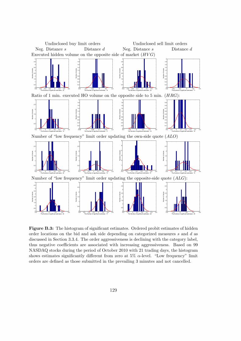
Undisclosed buy limit orders Undisclosed sell limit ordersNeg. Distance s Distance d Neg. Distance s Distance d
Executed hidden volume on the opposite side of market (HVG)
−0.8 −0.6 −0.4 −0.2 0 0.2 0.4 0.60
0.5
1
1.5
2
2.5
3
3.5
4
4.5
5
The Number of significant estimates: 23
Num
ber o
f sto
cks
−0.6 −0.4 −0.2 0 0.2 0.40
0.2
0.4
0.6
0.8
1
1.2
1.4
1.6
1.8
2
The Number of significant estimates: 14
Num
ber o
f sto
cks
−0.8 −0.6 −0.4 −0.2 0 0.2 0.4 0.60
0.5
1
1.5
2
2.5
3
3.5
4
4.5
5
The Number of significant estimates: 25
Num
ber o
f sto
cks
−0.6 −0.4 −0.2 0 0.2 0.40
0.2
0.4
0.6
0.8
1
1.2
1.4
1.6
1.8
2
The Number of significant estimates: 11
Num
ber o
f sto
cks
Ratio of 1 min. executed HO volume on the opposite side to 5 min. (HRG):
−0.2 −0.1 0 0.1 0.2 0.3 0.4 0.50
0.5
1
1.5
2
2.5
3
The Number of significant estimates: 14
Num
ber o
f sto
cks
−0.05 0 0.05 0.1 0.15 0.20
0.2
0.4
0.6
0.8
1
1.2
1.4
1.6
1.8
2
The Number of significant estimates: 11
Num
ber o
f sto
cks
−0.4 −0.2 0 0.2 0.4 0.60
0.2
0.4
0.6
0.8
1
1.2
1.4
1.6
1.8
2
The Number of significant estimates: 16
Num
ber o
f sto
cks
−0.2 −0.1 0 0.1 0.2 0.3 0.4 0.50
0.1
0.2
0.3
0.4
0.5
0.6
0.7
0.8
0.9
1
The Number of significant estimates: 10
Num
ber o
f sto
cks
Number of “low frequency” limit order updating the own-side quote (ALO)
−0.2 −0.1 0 0.1 0.2 0.3 0.4 0.50
0.5
1
1.5
2
2.5
3
The Number of significant estimates: 22
Num
ber o
f sto
cks
−0.3 −0.2 −0.1 0 0.1 0.2 0.3 0.40
0.5
1
1.5
2
2.5
3
The Number of significant estimates: 13
Num
ber o
f sto
cks
−0.2 −0.1 0 0.1 0.2 0.3 0.4 0.50
1
2
3
4
5
6
The Number of significant estimates: 27
Num
ber o
f sto
cks
−0.3 −0.2 −0.1 0 0.1 0.2 0.3 0.40
0.5
1
1.5
2
2.5
3
The Number of significant estimates: 15
Num
ber o
f sto
cks
Number of “low frequency” limit order updating the opposite-side quote (ALG):
−0.4 −0.2 0 0.2 0.4 0.60
0.5
1
1.5
2
2.5
3
3.5
4
4.5
5
The Number of significant estimates: 20
Num
ber o
f sto
cks
−0.8 −0.6 −0.4 −0.2 0 0.2 0.4 0.60
0.5
1
1.5
2
2.5
3
The Number of significant estimates: 17
Num
ber o
f sto
cks
−0.2 −0.1 0 0.1 0.2 0.3 0.4 0.50
0.5
1
1.5
2
2.5
3
3.5
4
The Number of significant estimates: 28
Num
ber o
f sto
cks
−0.4 −0.2 0 0.2 0.4 0.60
0.5
1
1.5
2
2.5
3
3.5
4
The Number of significant estimates: 25
Num
ber o
f sto
cks
Figure B.3: The histogram of significant estimates. Ordered probit estimates of hiddenorder locations on the bid and ask side depending on categorized measures s and d asdiscussed in Section 3.3.4. The order aggressiveness is declining with the category label,thus negative coefficients are associated with increasing aggressiveness. Based on 99NASDAQ stocks during the period of October 2010 with 21 trading days, the histogramshows estimates significantly different from zero at 5% α-level. “Low frequency” limitorders are defined as those submitted in the prevailing 3 minutes and not cancelled.
129

Undisclosed buy limit orders Undisclosed sell limit ordersNeg. Distance s Distance d Neg. Distance s Distance d
Number of fleeting orders on the own side of market (HFO):
−0.5 0 0.5 10
0.5
1
1.5
2
2.5
3
3.5
4
The Number of significant estimates: 24
Num
ber o
f sto
cks
−0.6 −0.4 −0.2 0 0.2 0.4 0.6 0.80
0.5
1
1.5
2
2.5
3
3.5
4
The Number of significant estimates: 17N
umbe
r of s
tock
s−0.5 0 0.5 10
1
2
3
4
5
6
7
The Number of significant estimates: 33
Num
ber o
f sto
cks
−1 −0.5 0 0.5 10
0.5
1
1.5
2
2.5
3
3.5
4
The Number of significant estimates: 18
Num
ber o
f sto
cks
Number of fleeting orders on the opposite side of market (HFG):
−0.5 0 0.5 1 1.50
2
4
6
8
10
12
14
16
18
The Number of significant estimates: 45
Num
ber o
f sto
cks
−0.4 −0.2 0 0.2 0.4 0.6 0.8 10
2
4
6
8
10
12
14
16
18
The Number of significant estimates: 41
Num
ber o
f sto
cks
−0.5 0 0.5 1 1.50
2
4
6
8
10
12
14
16
18
The Number of significant estimates: 61N
umbe
r of s
tock
s
−0.4 −0.2 0 0.2 0.4 0.6 0.8 10
2
4
6
8
10
12
14
16
18
20
The Number of significant estimates: 53
Num
ber o
f sto
cks
Opening hour (OPN):
−1.5 −1 −0.5 0 0.5 1 1.5 20
1
2
3
4
5
6
7
The Number of significant estimates: 32
Num
ber o
f sto
cks
−1.5 −1 −0.5 0 0.5 1 1.5 20
0.5
1
1.5
2
2.5
3
3.5
4
4.5
5
The Number of significant estimates: 39
Num
ber o
f sto
cks
−2 −1.5 −1 −0.5 0 0.5 1 1.50
1
2
3
4
5
6
The Number of significant estimates: 35
Num
ber o
f sto
cks
−1.5 −1 −0.5 0 0.5 1 1.5 20
1
2
3
4
5
6
The Number of significant estimates: 43N
umbe
r of s
tock
s
Closure hour (CLS):
−0.5 0 0.5 1 1.50
0.5
1
1.5
2
2.5
3
3.5
4
4.5
5
The Number of significant estimates: 18
Num
ber o
f sto
cks
−0.5 0 0.5 1 1.50
0.5
1
1.5
2
2.5
3
3.5
4
The Number of significant estimates: 24
Num
ber o
f sto
cks
−0.5 0 0.5 1 1.50
0.5
1
1.5
2
2.5
3
3.5
4
4.5
5
The Number of significant estimates: 21
Num
ber o
f sto
cks
−1 −0.5 0 0.5 1 1.50
1
2
3
4
5
6
The Number of significant estimates: 26
Num
ber o
f sto
cks
Figure B.4: The histogram of significant estimates. Ordered probit estimates of hiddenorder locations on the bid and ask side depending on categorized measures s and d asdiscussed in Section 3.3.4. The order aggressiveness is declining with the category label,thus negative coefficients are associated with increasing aggressiveness. Based on 99NASDAQ stocks during the period of October 2010 with 21 trading days, the histogramshows estimates significantly different from zero at 5% α-level. The fleeting order isdefined as the limit order cancelled in one second after the submission.
130

Selbstandigkeitserklarung
Ich bezeuge durch meine Unterschrift, dass meine Angaben uber die bei der Ab-fassung meiner Dissertation benutzten Hilfsmittel, uber die mir zuteil gewordeneHilfe sowie uber fruhere Begutachtungen meiner Dissertation in jeder Hinsicht derWahrheit entsprechen.
Berlin, 20 Dezember 2011
Ruihong Huang