an empirical study of the tea industry: inventory

CE

UeT

DC

olle

ctio

n

AN EMPIRICAL STUDY OF THE TEA INDUSTRY: INVENTORY MOVEMENTS ANDDEMAND

By

Tamas Zoltan Csabafi

Submitted To

Central European University

Department of Economics

In partial fulfillment of the requirements for the degree of Master of Arts in Economics

Supervisor: Attila Rátfai

Budapest, Hungary2010

CE

UeT

DC

olle

ctio

n

2

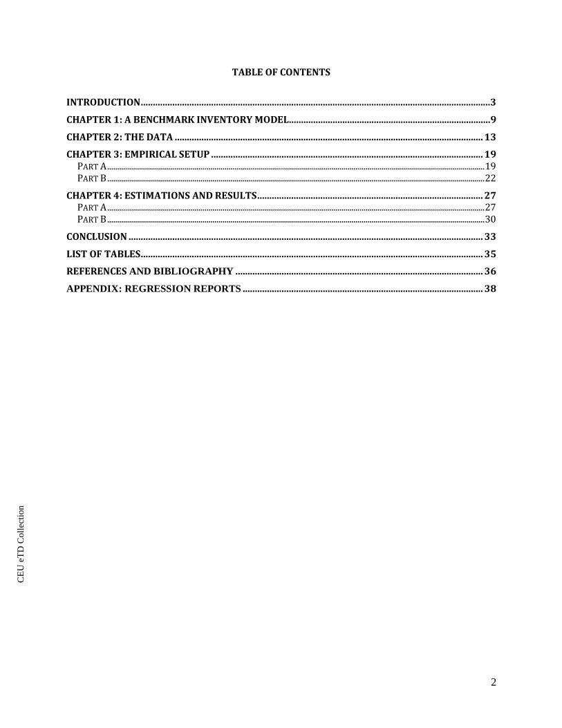
TABLE OF CONTENTS

INTRODUCTION................................................................................................................................................3

CHAPTER 1: A BENCHMARK INVENTORY MODEL...................................................................................9

CHAPTER 2: THE DATA ............................................................................................................................... 13

CHAPTER 3: EMPIRICAL SETUP ................................................................................................................ 19PART A..............................................................................................................................................................................................19PART B..............................................................................................................................................................................................22

CHAPTER 4: ESTIMATIONS AND RESULTS............................................................................................. 27PART A..............................................................................................................................................................................................27PART B..............................................................................................................................................................................................30

CONCLUSION .................................................................................................................................................. 33

LIST OF TABLES............................................................................................................................................. 35

REFERENCES AND BIBLIOGRAPHY ...................................................................................................... 36

APPENDIX: REGRESSION REPORTS ................................................................................................... 38

CE

UeT

DC

olle

ctio

n

3

Introduction

There has been an extensive literature that tried to grasp the role of inventory fluctuations in

the business cycle.1 Many attributed the surge in the GDP of the U.S. in the last quarter of 2009

to the rise of inventory levels in the wholesale and manufacturing sectors to before crisis levels.

This paper is aiming at evaluating the relationship between inventory levels and demands for

goods (sales) in the tea industry.

The economic importance of tea is not comparable to other commodities such as wheat,

coffee or gasoline in terms of consumption in absolute levels; however, it has similar features to

those mentioned. It is clearly similar to commodities as it is more or less homogeneous. There is

no difference biologically between tealeaves that are plucked, but through value added

production they are transformed into a limited number of beverages and products to consumers.

The case is the same for coffee or the different types of ores.

Tea furthermore has a health effect that is deeply rooted in the public awareness around the

globe. Unlike during the early 20th century, when good quality tea was only a beverage to the

higher classes and represented their status within society, nowadays, due to the open media it is

widely known that it is beneficial for overcoming a cold, losing weight, cleaning poisonous

material out of the blood flow, and helping in staying awake.

Due to multinational companies and their marketing activities, such as Lipton, Twinings,

Rauch, Nestle, tea consumption has become fashionable to some respect. It is relatively cheap to

acquire and available in nearly all grocery stores across world. As in the case of Hungary it is

also included in the measure of the CPI.

1 Blinder and Eakin (1984), Kahn (1990), Alessandria et al. (2008), Cooper and Haltiwanger (1983).

CE

UeT

DC

olle

ctio

n

4

Tea as a commodity, however, is produced in once-before colonial countries. The list

includes India, Sri Lanka, China, Kenya, Thailand, Indonesia, and South Africa. There are only a

few countries for, which the description would not fit, which include Japan and Turkey. Despite

the fact that in the tea producing countries the population drinks tea regularly, they are mostly

lagging behind per capita consumption compared to some European countries. It is not surprising

that the per capita consumption of tea is the highest in the United Kingdom with 2.1 kg per

person per annum in 2004.2

In order to fully grasp the underlying industry one has to be aware of the global structure of

it. Figure 1 depicts the setup of the global tea industry. There are three levels: the producers of

raw tea; the wholesalers who undertake production activities and create value added; and lastly

retailers, who sell directly to consumers. Besides the previously mentioned set up there is a

geographic constraint due climate restrictions. Tea can only be grown and harvested in tropical

and Mediterranean climates. This explains the restriction in the location of harvesters of raw tea

to former colonial countries mostly. Therefore, there is a shipment cost and a lag in acquiring the

raw tea. Also, it would make costs of acquisition of raw materials highly volatile due to fuel

prices. In reality, however, based on an interview conducted with a member of a large wholesale

company based in Hamburg, it can be stated that these costs are limited through contractual

arrangements with freight organizations.3 The usual timeframe of a contract is one year. Apart

from the shipment costs wholesalers are affected by weather shocks in producer countries of raw

materials. As this is an agricultural product seasonal weather has a large impact on the quantity

that could be sold to wholesalers in a given year. Dynamics of supply and demand tells one that

2 International Tea Committee – Annual Bulletin of Statistics 2009. Page 88.3 Interview conducted by the author with an employee of Wollenhaupt GmbH on April 25, 2010, in Vienna, Austria.

CE

UeT

DC

olle

ctio

n

5

this would have an effect on the price of raw tea. However, companies tend to overcome price

fluctuations by frame contracts for a given time period.

In the meantime, wholesalers undertake production activities that create value added. These

activities are filtering, packaging leaf teas, labeling, flavoring, and tea mixing. All these activities

require a set of machinery and other raw materials that are locally acquired. Such are packaging

materials, chemicals for flavoring, and paper for labels. As these are locally purchased they are

subject to inflation in the given country and overall price movements. These fluctuations are also

dealt with supplier contracts. They are minimized by company policy and persistence in the

prices of raw materials is present in the industry. For wholesalers, inventory management in this

sector is essential to meet consumer demand and orders and to minimize costs. As there is a large

delivery lag in receiving raw tea production is based on projections of demand for approximately

six months.

Consumer demand is highly volatile across countries and in time. In the time dimension it is

dependent on prices, weather conditions and trends in behavior. This last aspect is hard to grasp

in terms of models and this study will not deal with it in detail due to the lack of sufficient data.

An example on the Hungarian market occurred in 2007, when after a publication in Paramedica

newsletter in June orders for Java OP black tea increased substantially until the end of the

calendar year.4 Based on the calculations of this company based in Budapest, in 2007 sales of

Java OP black jumped to 118 kg from a mere 20 kg in 2006. The underlying article suggested

that black tea harvested on the island of Java had a beneficial effect to the body by lowering the

risks of cancer.5 Prices consumers face are more persistent than the acquisition prices. Prices are

4 Interview conducted by the author with the CEO of the tea wholesale company Possibilis Kft on May 20, 2010, inBudapest, Hungary.5 Ibid.

CE

UeT

DC

olle

ctio

n

6

determined on the basis of costs of production (including the acquisition of raw materials) and a

profit margin. The profit margins are usually large. Retail prices of this Hungarian company

from which I was able to collect data from include a margin 100 to 300 percent on its products

that include 340 different types of teas. Based on prices collected from an array of retail stores in

Budapest I have compared prices and concluded that they are tuned together.6 For the high

margin there are two reasons. One is that only a small quantity of tea can be bought. One tea

filter contains not more than 2 grams of tea and even in specialty stores 50 and 100 gram

packages are the standards.7 The second reason is that it enables retailers to endure idiosyncratic

and economy wide shocks without price adjustments upwards and this enables to maintain their

customer base in the long run. Lastly, the weather-based seasonality is an important factor of

demand each year in some countries. It has been a convention among tea wholesalers that they

publish new prices for the upcoming twelve months in August.8 Demand for tea is peaking

during the winter months. This is due to the fact that in most cultures that are located in the

continental climate stripes tea is a winter beverage. It is served warm and has beneficial effects

to one’s health. Its most commonly known feature is that it strengthens the immune system of the

human body when a bacterial or viral infection surfaces. It contains antioxidants, minerals and

teine9 that together have a cleaning effect on the digestive and cardiovascular system.

Furthermore, in December, Christmas has an effect on sales. High quality tea often serves the

purpose of a gift either in itself or as a supplement to kitchen accessories such as tea kits or

containers, mugs and porcelain items.

6 Interview conducted by the author with the CEO of the tea wholesale company Possibilis Kft on May 20, 2010, inBudapest, Hungary.7 Ibid.8 Interview conducted by the author with an employee of Wollenhaupt GmbH on April 25, 2010, in Vienna, Austria.9 Teine is a organic substance that has a similar effect on the body as caffeine. The underlying molecule is identical.

CE

UeT

DC

olle

ctio

n

7

Despite the above mentioned factors in prices, seasonality and cultural/health trends there is

an income effect that must be noted in terms of consumer demand. Large aggregate systemic

shocks to an economy, such as the recent financial crisis, have an effect on the income of

consumers. As in the case of Hungary wages have not been able to follow inflation in all sectors

and employment security diminished. More of one’s income is going towards savings and less to

consumption. Even within consumption funds available are drawn away from luxury and

expensive items that are not necessities. Tea as I have implied it before have features of a luxury

item. There are cheaper substitutes available in terms of its effects. Coffee and instant warm

drinks are the most significant ones. In the underlying tea company in Hungary a significant drop

occurred in all type of tea sales.10 A counteracting factor on the aggregate level could be that

cheaper and lower quality tea product sales increased.

Overall, the industry in its structural set up is not a complicated one, however, the factors of

supply and demand are heterogeneous. Consumer demand is volatile, which is attributable to

idiosyncratic and systemic shocks and prices, which in turn determines production by wholesale

companies. In the meantime, the volatility in the supply and price of raw tea is the most

important factors that determine corporate policy to match raw materials, production and

consumer demand in a timely and efficient manner, which makes the holding of inventories

imperative for firms in the industry.

In inventory movements there are two observations and results based on the literature that I

am going to evaluate using the data from the tea industry. One is that inventories are proportional

to sales. Two, there is a short-run trade-off between inventory investment and sales. These are

two statements that I am going to take a closer look at if they are applicable to the tea industry.

10 Interview conducted by the author with the CEO of the tea wholesale company Possibilis Kft on May 20, 2010, inBudapest, Hungary.

CE

UeT

DC

olle

ctio

n

8

The underlying studies of these findings mostly use firm level panel data to draw conclusions

from.11 My approach is bounded by the aggregate country level data I have available. Therefore,

I will test these results at the country level.

The further structure of this study is organized to revisit the above-described facts of

inventory movements and if they withhold in the tea industry. In Chapter 1, a model of inventory

management will be described based on Bils and Kahn (2000). I will give an introduction to the

model and describe its overall results relevant to evaluating the underlying issues. In Chapter 2,

two economic frameworks will be presented, which provide the backbone of the underlying

estimations and regressions. In Chapter 3, I will introduce the data I have gathered and used for

the purposes of this study and for the estimations. In Chapter 4, the results of the regressions and

estimations will be presented along with their implications.

11 The underlying studies that I used to evaluate the two issues after making adjustments to the empiricalframeworks they used are: Bils and Kahn (2000) and Choi and Kim (2001).

CE

UeT

DC

olle

ctio

n

9

Chapter 1: A Benchmark Inventory Model

In this Chapter I present a summary of the inventory model by Bils and Kahn (2000) and its

conclusions, which serves as a benchmark to compare the empirical findings based on my data

with.

As for the second benchmark model I will discuss the structure of Bils and Kahn (2000). The

model is built upon micro-foundations. The model of the authors suggest at the firm level that

firms’ demands for finished good inventories are proportional to their expected sale, however,

they remain countercyclical relative to sales during business cycles.12 The authors reject the

explanation for the cyclical nature of inventories that relies upon measured prices and

productivity. The countercyclical behavior of inventories as stated above require that during

expansionary periods firms exhibit high marginal cost relative to discounted future marginal

costs or low price markups giving way to inter-temporal substitution.

The patterns in fluctuations in the level of inventories thus can be explained by interpreting

fluctuations in labor productivity as a result of mis-measured cyclical utilization of labor, for

which the costs are internalized by the firms.13 The previous statement is also supported by the

findings of others that factors of production are worked more intensely in times of expansion.14

In the meantime, the underlying model provides a different explanation as well. The model

suggests that inventory behavior is primarily driven by countercyclical markups, which have the

12 Bils and Kahn (2000). Page 2713 Ibid. Page 27.14 The evidence is supported by the following studies: Burnside, Eichenbaum and Rebelo (1995), Bernanke andParkinson (1991), Shapiro (1993), Bils and Cho (1994).

CE

UeT

DC

olle

ctio

n

10

effect of changing the target inventory-to-sales ratio of the firm. As inventories are failing to

match orders by customers, the price of goods are unable to follow the marginal cost.15

The underlying model’s results on the aggregate level are the following: a rise in real

marginal cost, or equivalently a drop in the markup, directly reduces the value of inventory

holdings by reducing the valuation of sales generated by those inventories.16 Therefore the

cyclical behavior of inventory stock is the result of the variations in the target inventory-to-sales

ratio over the business cycle due to countercyclical markups.

The firm’s problem in this is a profit maximization framework, with a Cobb-Douglas

production function and inventory technology that reflects an inventory-to-sales ratio to be

independent of scale.17 This corresponds to a inventories of finished goods being productive in

generating larger sales at a given price.18

maxyt

Et t ,t i pt ist i Ct 1(yt i; t ; zt )i 1

subject toat it yt at 1 st 1 yt

yt minqt , ( tnt lt kt

1 )

st dt (pt )at

In the objective function, s and p stands for sales and price in period t; denote a technology

shock; and z is the vector of input price in period t. C(y) is the cost of producing the output y in

period t. is the discount factor at time period t for i periods ahead. As the authors point out this

refers to a nominal discount rate. It is also assumed that when firms choose production in t they

15 Bils and Kahn (2000). .16 Ibid. Page 4.17 Ibid. Page 4.18 These ideas are from the following studies: Kahn (1987) and Kahn (1992).

CE

UeT

DC

olle

ctio

n

11

know the realizations of the variables and z that determine the cost of producing, but not the

price or sales in the same period.19

The first constraint is a flow constraint of goods available for sale in period t, a. This consists

of the inventory stock carried forward from the previous time period and the goods produced in

period t. The second constraint is a specification of a production function. It entails that goods

are produced by using a vector of input materials, q, and value-added by a Cobb-Douglas

production function of labor, n, non-production labor, l, and capital, k. The parameter

determines the scale of the value added production function, which is greater than 1 in the

specification by the authors. Material inputs are proportional to output as dictated by a vector of

per unit material requirements, , which in the model is not a choice variable.20 The third

constraint specifies the relationship between finished inventories and sales of the firm. Subject to

the price in the given time period, the firm sees its sales as increasing with an elasticity of with

respect to its available stock for sale, where . The intuition behind this is that if the

elasticity is equal to 1, then a competitive firm can sell out all its available stock and a stock out

phase could occur. On the other hand if the elasticity is 0, then it would mean that production and

sales is only subject to cost-smoothing. Inventories in this model are viewed as an aggregate of

similar goods of different sizes, colors, locations...etc.21 Lastly, in the case when the elasticity of

the available goods is between 0 and 1 then a larger stock promotes matching with potential

buyers, who arrive with preferences for the specific type of good, however, the marginal benefit

of inventories diminishes in a relative to expected sales.22 Based on the panel data on US

19 Bils and Kahn (2000). Page 4.20 Ibid. Page 5.21 Ibid. Page 5.22 Ibid. Page 5.

CE

UeT

DC

olle

ctio

n

12

manufacturing industries by the authors, a trend is spotted that firms hold stocks of finished

inventories equivalent of one to three months’ worth of sales. Therefore, contrary to the

suggestion of the model (i.e. diminishing benefit of large stocks) that firms value inventories

beyond their role in varying production relative to sales.23

In the model demand for the producer is subject to the sales price of the goods produced,

d(p). This allows in a competitive setup that firm demand is determined by total supply and

consumer demand. In the absence of perfect competition the firms maximize the objective

function with respect to prices as well. This way the model is fit for mimicking a competitive and

a monopolistic industry as well.

Overall, the framework of Bils and Kahn is suitable for evaluating the trends of the tea

industry. It provides a set up in the absence of trade frictions just as if there were a just-in-time

system in place at the firms.

23 Bils and Kahn (2000). Page 6.

CE

UeT

DC

olle

ctio

n

13

Chapter 2: The Data

For the evaluation of the tea industry the focus will be on the aggregate country level data. I

used two sources for country level and trade data. One is a comprehensive database of the

International Tea Committee (ITC) based in London.24 From the ITC I have acquired ten years

long time series at the country level on imports/exports, sales/consumption and world prices

based on auctions in producing countries. The latter one covers a five-year long period only.

Furthermore, there is readily available data on consumption in the database of the Food and

Agriculture Organization (FAO) of the United Nations.

There are a number of limitations to the data available. First, the databases are not accessible

for the general public. In the case of the FAO only a limited number of queries can be initiated.

Regarding the ITC data, it is only made available in the form of publications for a relatively high

cost. Furthermore, the data that I have acquired differed in the level of detail compared to what I

have desired for. I have used the Annual Bulletin of Statistics (2009) of the International Tea

Committee. In the consumption and trade data there were no differentiation among the types of

teas. Initially I wished to differentiate between tea products along the major tea types (i.e. black

tea, green tea, Rooibush, mate tea and fruit mélanges), however, in the statistical bulletin there

was only data on aggregate tea levels and in some instances separately on black and green tea.

This fact limited my analysis to an aggregate analysis only.

24 International Tea Committee – Annual Bulletin of Statistics 2009 is the latest edition of a continuously updatedcomprehensive collection of data of the tea industry. It focuses on trade (export, imports, re-exports) andconsumption.

CE

UeT

DC

olle

ctio

n

14

Another limitation to the data available was the fact that aggregate or firm level inventory

stock data was only available for the United Kingdom through the UK Tea Council25, which is

the official regulatory body of the tea industry in the UK. This created a problem that apart from

one country I lacked the data on beginning inventory levels. I overcame this obstacle by

calculating the ratio of end of period inventory to consumption, which was 2.69. This means that

at the end of the first period inventories were 2.69 times larger than the consumption for that

period. Furthermore, I made the assumption that this ratio was representative of the countries in

my sample. Therefore, I calculated the first end of period inventory levels by multiplying the

consumption in that period by 2.69. The first beginning of period inventories I calculated by

subtracting the consumption in the first period from the end of period inventories for all

countries.

There are 15 countries in the dataset I used that are all importing and consumer countries of

tea. In reality, some of these countries re-export tea after adding some value added to it,

however, I omitted re-exports. The reason for the omission was that the underlying empirical

models I intend to use do not allow for re-exports. As the countries are not harvesting ones, they

import the majority of tea for consumption. The countries included in the sample are the

following:

1 - Austria2 - Czech Republic3 - Denmark4 - Finland5 - France6 - Germany7 - Ireland8 - Italy9 - The Netherlands10 - Norway

25 The data was available only through the International Tea Committee.

CE

UeT

DC

olle

ctio

n

15

11 - Poland12 - Switzerland13 - Canada14 - U.S.15 - United Kingdom

The available data included 10 years long monthly frequency time series of sales and imports

for the above listed countries only. Time series of sales and imports for consumption provided

the basis for calculating the corresponding beginning and ending of period series provided the

initial calculations mentioned above for the starting values of inventories. The assumption that

the ratio of consumption to inventories in the UK is representative of the sample countries is

based on the notion that most of them are a part of the developed world based on their income in

1998 in current international dollars based on PPP:26

Table 1 - GDP per Capita of Selected Countries in 1998

Country GDP per capita (current int’l dollars– PPP)

Austria 25,959

Canada 25,608

Czech Republic 13,777

Denmark 25,964

Finland 21,630

France 23,613

Germany 24,216

Ireland 23,588

Italy 22,526

Netherlands 26,815

26 IMF - World Economic Outlook Database April, 2010 - GDP based on purchasing power parity per capita incurrent international dollars.

CE

UeT

DC

olle

ctio

n

16

Norway 36,290

Poland 9,073

Switzerland 28,826

United Kingdom 23,251

United States 31,858

The outliers in the group are Poland and the Czech Republic with substantially lower per

capita income. However, it can be seen that over the course of ten years these countries have

been able to close up on the gap somewhat. There are two more outliers but in the opposite

direction. Norway and the United States have significantly higher GDP per capita than the

average of the group at 24,200 dollars. However, my initial assumption is reasonable based on

the cultural feature of these two countries that none of them are culturally prone to consume tea.

Table 2 displays the summary of the descriptive statistics of the main variables in level terms

(log terms). From this it can be concluded that the level of inventories is more volatile than the

levels of sales across countries and time. The same can be determined from the standard

deviations of the growth rates (log difference variables), namely, the growth rate of inventories is

more volatile than the growth rate of sales. The inventory-to-sales ratio has a mean of 3.54 across

the sample.

Table 2 - Descriptive Statistics 1.

N(no. of obs.) Mean Standard

Deviation Median

ln S(i,t) 1800 6.4217 1.5339 6.4134

Inv (i,t)/S(i,t) 1800 3.5417 3.2171 2.8934

ln Inv(i,t) 1800 7.3474 2.0603 7.7943

dln S(i,t) 1785 0.000567 0.1007 -0.00868

dln Inv(i,t) 1683 -0.001056 0.2366 0.00134

CE

UeT

DC

olle

ctio

n

17

The above data and methods to construct series of inventories for the beginning and end of

period are used in framework of Part A of Chapter 3. However, the time series across countries

are also used to estimate the demand equation for tea across countries based on a simple model

of Part B of Chapter 3.

For the purposes estimation I use the time series of sales across countries directly in the

empirical evaluations, meanwhile, import data is only used to construct a beginning of period

inventory measure. For this I used the previously determined ratio of UK end of period

inventories relative to sales in the same period. Then I multiplied the first month sales figure by

this number (2.69) and added the actual sales and subtracted the import numbers to get inventory

figures for the beginning of the first month, which happens to be January of 1998. After that I

constructed beginning of period inventory series for each country by adding imports and

subtracting exports from beginning inventory stocks to get the next period beginning inventory

stock. This is line with the model’s inventory stock flow constraint in Chapter 3 part (B):

Furthermore, the ITC Annual Bulletin of Statistics contained monthly average prices of all

tea types from the major auction markets in the world. These included Chittagong, Colombo,

Jakarta, Mombasa, Limbe, Kolkata and Guwahati. I chose the prices from the Jakarta auction

market as trading is done in US dollars and the turnover in trade quantity is among the top three

auction markets in my sample of auctions. The time series of prices begin in January 2005 and

end in December 2008, which are 48 observations. Therefore, I used equivalently 48

observations from other series (sales, beginning of inventory stock) for the same time period to

be consistent.

CE

UeT

DC

olle

ctio

n

18

From the statistical summary below one can grasp that inventories are the most volatile

with standard deviation of 9132 tons. Also, the average monthly level of inventory is

approximately three times larger than that of sales in the period. Prices are the least volatile.

Table 3 - Descriptive Statistics 2.Mean Median Standard Deviation

Sales 1983 657 3296Beginning of Period

Inventory6389 2813 9132

Acquisition Price of 1ton of Tea

1309 1340 205

Finally, from the serial correlation matrix one can see that sales and inventory stocks are

relatively highly correlated; meanwhile, prices are lowly correlated with sales and inventory

stocks. Hereby it must be noted that the data for global prices is a rough proxy of actual ones. As

described in the introduction it is only related to a ton of tea and shipment costs are, for instance

are assumed away for further analysis.

Table 4 - Serial Correlation MatrixSales Beginning of Period Inventory Acquisition Prices

Sales 1.0000

Beginning of Period Inventory 0.8732 1.0000

Acquisition Prices -0.0036 -0.0031 1.0000

In summary, I used the same monthly ten years long country level series for all of my further

estimations. There is difference in the calculation of the inventory stock series for beginning and

ending of each period that are in line with the respective frameworks in the following chapter.

Furthermore, in the latter case the time series across countries were only 48 periods long instead

of 120 due to the limitations of available price data.

CE

UeT

DC

olle

ctio

n

19

Chapter 3: Empirical Setup

In this Chapter I will present two frameworks for testing the implied relationships based on

the model in Chapter 1. The first framework is aimed at evaluating the determinants of inventory

levels, meanwhile, in the second part of this Chapter I present a simple partial equilibrium model

of a representative firm through which I intend to evaluate the determinants of the demand for

tea.

Part A

In the following framework the demand for inventories is determined by a number of

motives. First, there are the motives of avoiding a stock-out, smoothing production and meeting

orders. The latter as it has been established in the introduction is the one most important

determinant of inventory demand. Inventories comprise of goods and raw materials for

production. Here I must make a simplification as a result of the feature of production in the tea

industry. The raw material is equivalent in quantity to the finished good. There is mostly only

value added production in the form of flavoring and packaging. As in terms of quantity raw

materials and finished goods are equal. I further assume that other raw materials are negligible in

terms of quantity and costs. Based on this, I make the assumption that in each period, production

equals raw materials in quantity. The only major difference is in the price of acquiring the raw

tea and the sales price.

As for the framework, I assume that the representative firm chooses inputs, including

inventories at the beginning of each time period. In the beginning of each period the firm also

chooses its level of production. Furthermore, the firm chooses the inventory investment outright

at the start of the period. It should be noted that in this framework there are no delivery lags.

CE

UeT

DC

olle

ctio

n

20

Total output therefore corresponds with the sum of inventory investment and the output of

finished goods, which are equal in quantity.

- represents the output of the representative firm. This means, for example, in the case of the

tea industry that if a firm orders 100 tons of raw tea, then the output in that period will be a 100

tons of tea available for sale, packaged and flavored. Here it does not make sense to mark

inventory investment as a different variable from output unlike in the case of delivery lags.

Production function is homogeneous of degree one where the quantities of output and input

linearly related.

- marks the quantity of inventory carried forward from the previous period. In the

framework it is also not reasonable to distinguish between inventories of raw materials and

finished goods as result of the nature of the production technology that is also in line with our

assumptions. This variable is also measured in tons of tea.

- stands for the beginning of period inventory of tea measured in tons. It equals the

inventories carried forward from the previous period plus inventory investment, which equals

output.

- is the total sales of tea in a given period. It is measured in tons.

- this variable marks the end of period inventory in tons of tea. It equals the beginning of

period inventory minus sales.

CE

UeT

DC

olle

ctio

n

21

Altogether planned inventory investment is made up of outright investment (output) in each

period less sales. Also, in line with Choi and Kim (2001) and Bils and Kahn (2000) it can be

stated that output should respond more than proportionately to sales.

Now let us turn to the empirical model specification. In the above framework it has been laid

down that sales have a positive relationship with inventory levels. First, I am going to take a look

at this relationship with a simple panel regression with inventories as the dependent variable and

sales as the independent variable.

There is also a time varying parameter in that could cover and reflect the effects and

changes in inventory management over time. Furthermore, it is easy to see, as it has been implied

by Bils and Kahn (2000), that if the inventory-to-sales ratio is stable across time, then should

equal 1.27

As a further step, I am specifying a more complex inventory adjustment model. In this

regression the dependent variable is the change in the level of inventories. Regarding the

explanatory variables, since the previous regression implies that firms manage and implement

changes in inventories to close the gap between the target inventory-to-sales ratio and the actual

one, I have included a lagged version of the inventory-to-sales ratio on the right hand side.

Among the explanatory variables there is the change in the real inventory stock and that of sales.

27 Based on Choi and Kim (2001) page 7.

CE

UeT

DC

olle

ctio

n

22

The coefficient of the lagged inventory-to-sales ratio is expected to be negative because if

there is a target ratio and there is a rise in the actual one then a negative adjustment follows in the

next period. This is implied by the notion that firms in the industry are maintaining a stable ratio.

Now turning to movements in sales, with an unexpected jump in sales inventories would

adjust downwards. This would be a result of the role of inventories as a buffer stock, i.e.

counteracting a sales shock. The lagged sales growth may have a negative coefficient as well, as

a result of the time firms need to adjust inventories through changing raw material orders and

production.

Part B

As the next step I introduce another simple framework to assess the relationship of

inventories to sales and acquisition prices. This is a simple model resembles the features of the

partial equilibrium model setup of Bils and Kahn (2000) by focusing solely on the representative

firm’s problem. In this model the representative firm could be viewed as one large firm

representing a country. The firm maximizes profits subject to a production and an inventory

technology. My overall goal is to estimate a demand function that is subject to inventory stocks

and global prices to get a deeper insight into the relationship of sales and inventories.

The firm has a production function that is homogeneous of degree one and output and

imports, which represent the only input into production, are linearly related. This means as in the

previous case that one unit of output is gained from one unit of input, which is in our case, is one

ton of raw tea. The objective function and maximization problem looks as the following:

CE

UeT

DC

olle

ctio

n

23

maxpi ,t ,si ,t ,mi ,t ,ai ,t

EtT pi,t T si,t T zi,t T mi,t T ai,t

T 0

subject tosi,t A i,t pi,t ai,t

ai,t 1 ai,t si,t mi,t

In the objective function and represent sales prices and sales respectively, meanwhile,

is the acquisition price of the input . The acquisition price is based on global prices from

the auction in Jakarta. I chose the Jakarta tea auction market because the currency of trading is

the US dollar and by turnover of trading it is among the top three auctions in the world. Due to

the fact that I assume that firms acquire inputs on global prices there are no cross-country

differences in this cost. The firm also has to endure a each period a fixed cost of storage cost that

is always a fixed portion, , of the inventories, , in the beginning of the period. The firm

therefore makes sales at a given price in each period to generate revenues, meanwhile, endures

the acquisition costs of inputs and a fixed cost of production.

The first constraint determines the demand for the product of the company, which is in our

industry case, is tea. The demand is depending on inventories and the sales price. For a given

price, a producer views its sales as increasing with an elasticity of with respect to its available

stock, where .28 This parameter’s role is identical to that in the original model of Bils

and Kahn (2000). It allows in a competitive case for stock-outs at one extreme when the

elasticity is equal to one. On the other extreme case when the elasticity is equal to 0 it represents

a case of a pure cost-smoothing model. When the elasticity is in between zero and one then

larger inventory stock promotes matching of products with buyers with given preferences, which

28 Bils and Kahn (2000). Page 5.

CE

UeT

DC

olle

ctio

n

24

entails that the marginal benefit of this matching process diminishes in the inventory levels

relative to sales.29

As pointed in the previous description of the data available in the UK in January of 1998 held

2.69 times more inventories in the end of the month than the actual sales of tea in the same

month. This is in line with the findings and data of Bils and Kahn (2000), who suggest that

typically firms hold stocks of finished inventories that are equivalent of one to three months’

worth of sales.30

The demand for tea moves proportionately with a stochastic function of ,

where A is a scale parameter, is stochastic demand shock, which I assume to be an i.i.d.

process for the sake of simplicity. Furthermore the parameter captures price elasticity, which is

identical across countries.

The second constraint is a simple flow equation that determines the next period’s beginning

inventories. The beginning inventory is determined by the beginning inventory in the current

period plus inventory investment (acquisition of inputs in this case) from which we subtract the

sales in the current period.

After describing the setup of the model one can derive the first order conditions. The first

order conditions are the following:

29 Bils and Kahn (2000). Page 5.30 Ibid. Page 5.

CE

UeT

DC

olle

ctio

n

25

From the first order conditions we can see that after differentiating with the control variables

import term falls out. Combining equations (1), (2) and (3) and some straightforward

manipulations we can derive the constant markup over the acquisition price from which we make

the assumption that firms across countries charge a constant markup over the acquisition cost of

inputs. This is enabled by our simple production technology. The markup is the following:

As input prices are identical to firms in all countries and there is a constant markup policy in

determining sales prices we can conclude that sales prices in this model are the same across

countries and it only differs across time. Now let us denote the markup by capital M. Now, using

equation (1), (2) and (5) we can derive an equation that determines the inter-temporal

substitution of holding inventories.

This equation tells us that cost of holding one extra unit of inventory equals the present value

of the fixed cost of holding one unit of inventory and the acquisition cost, which is equal the

benefit of it in the next period that is coming from sales.

After laying down the optimality conditions for the firm now we can turn turn to estimating

the demand for the underlying good of the firm. We derive the final equation that is to be

CE

UeT

DC

olle

ctio

n

26

estimated by substituting (5) into the demand equation and then taking the natural logarithm of

both sides. This way we get the following logarithmic demand equation:

This is the demand equation that I will estimate. On the left hand side there is the level of

sales, which is dependent on a sales/demand shock, , with an expected value of 0 as it is an

i.i.d. process across countries; a constant term, , that accounts for the cross-

sectional fixed effects across time; and the level of prices and inventories in the same time

period. As the expected value of the sales/demand shock is zero the final model specification will

be the following:

In line with my model and that of Bils and Kahn (2000) I expect that the relationship

between levels of sales and inventories will be positive but less than proportional, meaning, that

the coefficient remains between 0 and 1, which would reflect a diminishing marginal benefit

from holding inventories. This would also provide evidence for a sluggish co-movement of sales

with increasing inventories. As for the price elasticity of input prices I expect it to be larger than

unity based on the assumption that tea is a normal good and there is a constant markup

determined by the price elasticity.

CE

UeT

DC

olle

ctio

n

27

Chapter 4: Estimations and Results

In this Chapter I will report the results of the regressions and interpret them in the light of my

expectations and the results of the benchmark model of Bils and Kahn (2000). In addition, I will

discuss qualitatively the differences in the outcomes of the regressions compared to the models.

Part A

It is the aim of my first regression to determine if there is a close link between the levels of

inventories and sales, as it has been suggested by the target inventory benchmark model of

Chapter 3. I performed the regression first by using a pooled OLS method and fixed effect

estimation method. The results are presented in the table below.

Table 5 - OLS and 2SLSPooled OLS 2SLS

Constant 0.1221(0.6933)

-0.00518(0.7614)

lnSales 1.1190(0.0892)

1.1323(0.0954)

R-squared 0.70 0.68

N 1719 1539

Results of the pooled OLS regression confirm the expected relationship between the levels of

sales and inventories. The adjusted is 0.70 and the estimated coefficient of the level of sales is

close to unity. The coefficient for sales is significant at the 5 percent significance level. These

results are in support of the relationship between sales and inventories that suggests that firms at

a country level hold inventories roughly proportional to sales over time.

CE

UeT

DC

olle

ctio

n

28

For the purpose of robustness check I have estimated the inventory-sales relationship with a

two stage least squares method to control for the possible biases that could arise from the

correlation of the regressor and the error term. This scenario could arise if the firms of a country

in the sample would target expected sales instead of using actual sales as in our case. To control

for such a bias with 2SLS method using the 12 lags of the explanatory variable as instruments.

This way as it can be observed from the above table that this method yields almost the same

results with a coefficient for the level of sales above one, meanwhile, being statistically

significant. The R-squared is 0.68, which is close to the result of the pooled OLS result of 0.70.

Based on the results of these two regression it can be established that firms in these countries

more or less keep inventories roughly proportional to sales in the tea industry. This evidence is in

line with the findings Bils and Kahn (2000) and Choi and Kim (2001) on durable good producing

industries and S n P 500 firms.

In the specification of the regression for dynamic adjustment of inventories is specified in the

difference of the levels of inventories. In this I have ran the regressions to determine the effect of

sales growth. Furthermore, I have looked at the effects of inventory investment and the

inventory-to-sales ratio. I used fixed effect estimation method once without adding time

dummies and including them as well.

With regards to the sales growth effect on inventory investment there are somewhat different

results. In case when there are no dummies in the specification the current period sales growth

reduces inventory investment, meanwhile, the one period lagged one increases. In case of both

variables the results are statistically significant at the 5 percent level. At the same time, when the

time dummies are included in the regression and accounting for the country level fixed cross-

section effects across time, then both the current and the lagged coefficient of the sales growth

CE

UeT

DC

olle

ctio

n

29

are negative, which would be in support of the role of inventories as a buffer stock. In other

words this would provide evidence for the production-smoothing role. However, it must be noted

that only the coefficient of the current sales growth is statistically significant.

In both specifications the lagged dependent variable on the right hand side has a positive

coefficient 0.19 and 0.21 respectively. Both are statistically significant which suggests that over

time there is no adjustment with oscillation as in the findings of Choi and Kim (2001). This

means that if previous period inventory growth is larger by one unit then current period

inventory growth will be larger by 0.2 approximately ceteris paribus. The coefficient of the

lagged inventory-to-sales ratio is in both cases is negative but statistically not significant. The

negative coefficients in themselves would provide evidence in support of inventory adjustment in

line with inventory-to-sales targeting.

Table 6 - Fixed Effect Estimation of Dynamic SetupFixed Effect w/o Time Dummies Fixed Effect with Time

DummiesConstant 0.0254

(0.0284)0.0929

(0.0569)ld_Sales -0.3581

(0.0960)-0.6608(0.3777)

ld_Sales_1 -0.1827(0.0463)

-0.1140(0.2845)

l_InvSalesR_1 0.0320(0.0285)

-0.0247(0.0248)

l_Inv_end_1 0.1944(0.0870)

0.2089(0.0813)

N 1656 1656Adjusted R-square 0.0820 0.1432

In summary, using the data from the ITC database for the static empirical model based on the

first framework found evidence for a positive close to proportional (a bit more) relationship

between the levels of sales and inventories. This is in support of the findings of Bils and Kahn

(2000). Therefore, in the tea industry on the aggregate level inventories move proportionally to

CE

UeT

DC

olle

ctio

n

30

actual sales. In the meantime, based on the dynamic empirical model specification the inventory-

to-stock ratio shows a positive relationship with inventory growth in the tea industry, which

would provide evidence against adjustments with oscillations as in Choi and Kim (2001),

however, the results are not conclusive as they fail to be statistically significant.

Part B

Based on the simple model of Chapter 4 part (B) here I will estimate the parameters of the

demand equation as specified by equation (8) for the tea industry:

The data is 48 observations per variable for 15 countries. The dependent variable is the level

of sales. The constant term accounts for any cross sectional fixed effects across time, meanwhile,

the explanatory variables are the levels of inventories and the global price level of tea. I

estimated the parameters with pooled OLS regression and fixed effect panel method for which

the results are summarized in the table below.

Table 7 - Demand Equation EstimationPooled OLS Fixed Effect Estimator

Constant 1.1089(1.9542)

6.3075(4593)

z(t) 0.0505(0.1936)

-0.0117(0.0555)

a(i,t) 0.6679(0.1073)

0.05048(0.0121)

N 605 605

Adjusted R-squared 0.7439 0.989261

CE

UeT

DC

olle

ctio

n

31

In both estimations the coefficient of the level of inventory levels is positive and between

zero and one, which is in line with our expectations. With both methods the results are

significant at the 5 percent level. This indicates to the fact that based on the original benchmark

model inventories in the tea industry are not solely used as a buffer stock but also to gain the

marginal benefit of matching buyers preferences.

However, the results of the two estimation methods differ greatly in terms of the coefficient

of the level of global prices (which represents the price elasticity as well). In case of the pooled

OLS the coefficient is positive, meanwhile, statistically not significant. This would mean that by

1 percent increase in the global acquisition price of raw tea sales level would increase by 0.05

percent. Even though it is close to zero there would still be an attenuation bias upwards

stemming from the fact that the Jakarta monthly average prices are very rough proxies of actual

global prices. In the meantime, the fixed effect method estimated a negative coefficient,

however, it remained below unity, which fails to meet expectations. The estimate of the price

coefficient is also fails to be significant statistically. Again the inconsistency of the estimation

method can be a result of attenuation bias in this case as well and that is why this coefficient has

been underestimated.

In comparison the fixed effect estimation method had a higher explanatory value with an

adjusted R-square value of 0.98, meanwhile, the pooled OLS performed reasonably as well with

an R-square value of 0.74. Overall, the fixed effect estimator performed better than pooled OLS.

In conclusion, I could not confirm all the implications of my simple model on consumer

demand. The results of both estimation methods indicated that the relationship between the level

of sales and level of inventories is withstanding and significant statistically. This means that in

the tea industry inventories serve different purposes at the same time such as a buffer stock role

CE

UeT

DC

olle

ctio

n

32

and enabling the firm to meet consumer preferences and by that gaining the marginal benefit of

storing an extra unit of it, however, as the below unity coefficients may indicate there is a

diminishing marginal benefit over having an extra unit stored. In the meantime, the results on the

coefficient of the global prices are mixed. The fixed effect estimator performed clearly better but

failed to meet the expectations based on the simple model. In any case, both of the fixed effect

method and the pooled OLS was inconsistent. Based on reviewing the literature and similar

studies I have come to the conclusion that based on my studies I lacked the technical knowledge

to perform a more sophisticated estimation method such as the GMM, which has also been used

by Bils and Kahn (2000) to estimate their model parameters. A further limitation to perform

more accurate and consistent estimates was that especially in terms of prices the data available

for use was very rough and possibly not fully representative of global tea prices on average.

CE

UeT

DC

olle

ctio

n

33

Conclusion

In conclusion, this thesis attempted at determining if two statements are applicable to the tea

industry with regards to inventory movements. One was the statement that inventories are

proportional to sales; meanwhile, the other tried to grasp a short-run trade-off between inventory

investment and sales.

The simple inventory flow approach with a modified empirical setup of Choi and Kim (2001)

provided evidence that the level of sales have a positive proportional relationship to the level of

inventory on an aggregate level. A dynamic setup based on the same approach, however, yielded

somewhat mixed results. The inventory-to-stock ratio showed a positive, but statistically not

significant, relationship with inventory growth in the tea industry. Therefore, I could not draw

definite conclusion regarding the second statement. The estimation results did not confirm the

initial statement on the trade-off between inventory investment and sales.

To further analyze the relationship of inventories to sales I have developed a simple partial

equilibrium model based on the model of Bils and Kahn (2000). The model of the paper is

simply put a modified version of the original model. Here I intended to take a look at the

relationship of inventory stock and sales through estimating a demand equation. In this model a

constant mark-up was on sales prices and they depended on input prices only due to the linear

production technology, which was HOD 1. The results were mixed here as well. The estimation

by fixed effect and pooled OLS methods confirmed that the level of inventory had a positive

relationship with sales demand; however, it did not confirm a proportional relationship. In terms

of acquisition prices, only one estimation method gave a negative relationship, but it was not

statistically significant. Overall, both approaches provided some evidence in support of the two

statements, but failed to confirm the proposed relationships without doubt.

CE

UeT

DC

olle

ctio

n

34

In this part of the thesis I would like to summarize the issues that arose during the research

and might have an effect on the end result. First of all, I would like to mention the problem of

lack of data. There has only been aggregate country level data available through the International

Tea Committee and the Food and Agriculture Organization of the UN. Furthermore, price data

has only been available from tea auction markets and not from other representative sources.

These issues limited my evaluation and likely yielded a bias in the data and thus in the

estimations. A technical issue arose when I chose the estimation methods. The lack of knowledge

of advanced econometrics limited the list of possible estimation methods and as a result I could

not implement GMM estimation in the case of the demand equation estimation as in the study of

Bils and Kahn (2000).

Finally, I would like to share my thoughts on how this research could be brought forward. A

first possibility would be to acquire firm level data. I have attempted to get data from the

wholesale company Wollenhaupt GmbH, but for understandable reasons I have been turned

down. Firm level data would enable to get a more accurate picture of inventory movements in

the tea industry. Following from the previous point a more complex production function and a

more detailed pricing mechanism could be estimated, which would enable more accurate results.

The relevance of the tea industry lies in the fact that it is an agricultural product and is subject to

a vast number of threats during storage and shipment. Like in Alessandria et al. (2008) the

introduction of delivery lags and shipment costs could further clarify the picture. What is the

relationship if inventory levels and sales given the proposed tracks for further research be it in

the form of the introduction of frictions or better quality data.

CE

UeT

DC

olle

ctio

n

35

List of Tables

Table 1 - GDP per Capita of Selected Countries in 1998 ...........................................................15Table 2 - Descriptive Statistics 1. ..............................................................................................16Table 3 - Descriptive Statistics 2. ..............................................................................................18Table 4 - Serial Correlation Matrix............................................................................................18Table 5 - OLS and 2SLS ...........................................................................................................27Table 6 - Fixed Effect Estimation of Dynamic Setup.................................................................29Table 7 - Demand Equation Estimation .....................................................................................30

CE

UeT

DC

olle

ctio

n

36

References and Bibliography

- Alessandria, G. – Kaboski, J. – Midrigan, V. “Inventories, Lumpy Trade, and LargeDevaluations,” NBER Working Paper, Working Paper No. 13790, February 2008.

- Bernanke, Ben and Parkinson, Martin. “Procyclical Labor Productivity and CompetingTheories of the Business Cycle: Some Evidence from Interwar U.S. ManufacturingIndustries,” The University of Chicago Press, The Journal of Political Economy, Vol. 99,No. 3 (Jun., 1991), pp. 439-459.

- Bils, Mark and Cho, Jang-Ok. "Cyclical factor utilization," Discussion Paper / Institutefor Empirical Macroeconomics 79, Federal Reserve Bank of Minneapolis, 1993.

- Bils, Mark and Kahn, James. “What Inventory Behavior Tells Us About BusinessCycles?” The American Economic Review, Vol. 90, No. 3 (Jun., 2000), pp. 458-481.

- Blinder, S. Alan. “Inventories and Sticky Prices: More on the Microfoundations ofMacroeconomics,” American Economic Association, The American Economic Review,Vol. 72, No. 3 (Jun., 1982), pp. 334-348.

- Blinder, S. Alan and Eakin, H. Douglas. “Inventory Fluctuations in the United StatesSince 1929,” NBER Working Paper, Working Paper No. 1371, June 1984.

- Burnside, Craig – Eichenbaum, Martin – Rebelo, Sergio. “Capital Utilization andReturns to Scale,” NBER Macroeconomics Annual, Vol. 10, (1995), pp. 67-110.

- Choi, Woon Gyu and Kim, Yungsan. “Has Inventory Investment Been Liquidity-Constrained? Evidence from U.S. Panel Date,” IMF Working Paper, August 2001.http://www.imf.org/external/pubs/ft/wp/2001/wp01122.pdf. Visited on April 30, 2010.

- Chambers, J. Marcus and Bailey, E. Roy. “A Theory of Commodity Price Fluctuations,”The University of Chicago Press, The Journal of Political Economy, Vol. 104, No. 5(Oct., 1996), pp. 924-957.

- Cooper, Russel and Haltiwanger, John. “Inventories and the Propagation of SectoralShocks,” American Economic Association, The American Economic Review, Vol. 80,No. 1 (Mar., 1990), pp. 170-190.

- Kahn, A. James."Inventories and the Volatility of Production," American EconomicReview, American Economic Association, vol. 77(4), pages 667-79, September 1987.

- Kahn, A. James. "Moral hazard, imperfect risk-sharing, and the behavior of assetreturns," Journal of Monetary Economics, Elsevier, vol. 26(1), pages 27-44, August1990.

CE

UeT

DC

olle

ctio

n

37

- Kahn, A. James. "Why Is Production More Volatile Than Sales? Theory and Evidence onthe Stockout-Avoidance Motive for Inventory-Holding," The Quarterly Journal ofEconomics, MIT Press, vol. 107(2), pages 481-510, May 1992.

- Ramey, A. Valerie. “Inventories as Factors of Production and Economic Fluctuations,”American Economic Association, The American Economic Review, Vol. 79, No. 3 (Jun.,1989), pp. 338-354.

- Interview conducted by the author with Dr. Csabafine Mezei Maria the CEO of the teawholesale company Possibilis Kft. on May 20, 2010, in Budapest, Hungary.

- Interview conducted by the Daniel Kany an employee of Wollenhaupt GmbH on April25, 2010, in Vienna, Austria.

- International Tea Committee, Annual Bulletin of Statistics 2009, Published by theInternational Tea Committee Ltd., London, UK, 2010.

- FAOSTAT Website, Food and Agriculture Organization, United Nations Organization,http://faostat.fao.org/default.aspx. Visited on May 25, 2010.

- World Economic Outlook Database 2010, International Monetary Fund.http://www.imf.org/external/pubs/ft/weo/2010/01/weodata/weoselgr.aspx. Visited onJune 5, 2010.

http://faostat.fao.org/default.aspx

http://www.imf.org/external/pubs/ft/weo/2010/01/weodata/weoselgr.aspx

CE

UeT

DC

olle

ctio

n

38

APPENDIX: Regression Reports

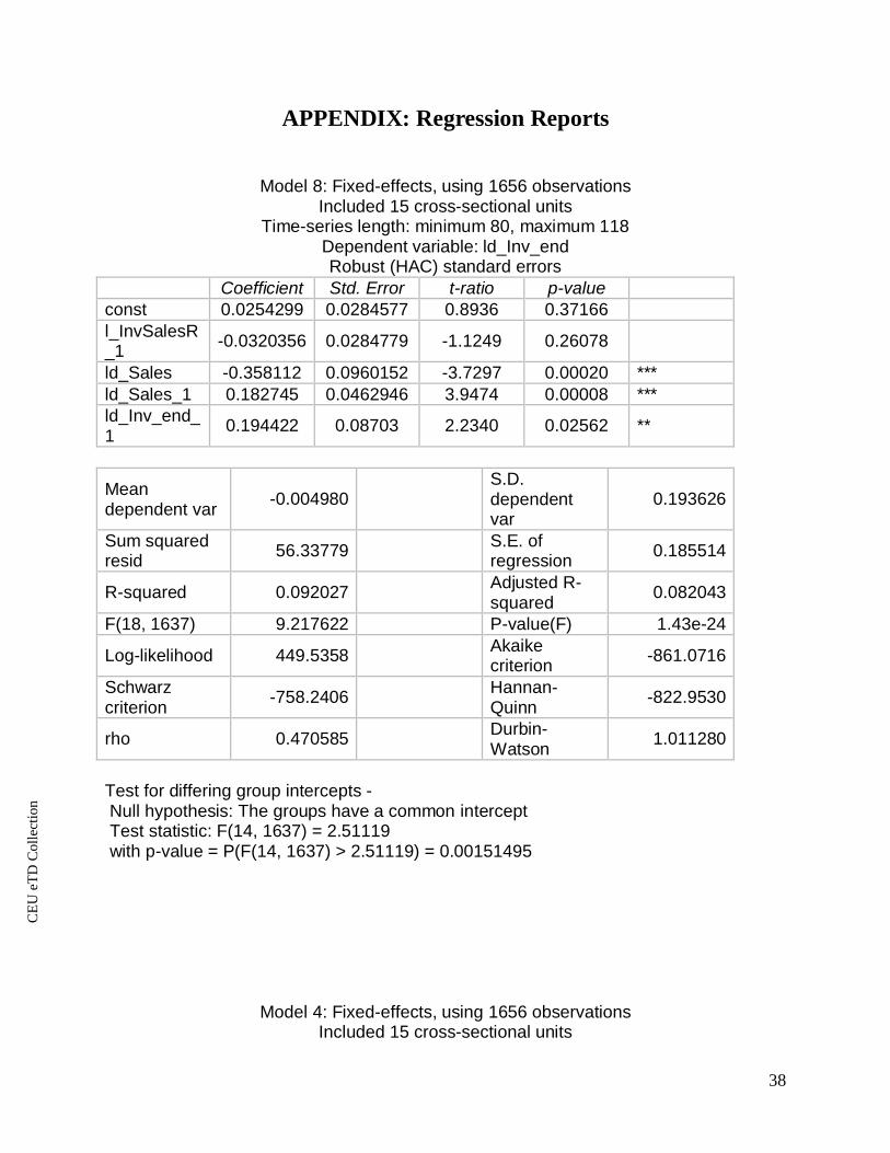
Model 8: Fixed-effects, using 1656 observationsIncluded 15 cross-sectional units

Time-series length: minimum 80, maximum 118Dependent variable: ld_Inv_endRobust (HAC) standard errors

Coefficient Std. Error t-ratio p-valueconst 0.0254299 0.0284577 0.8936 0.37166l_InvSalesR_1 -0.0320356 0.0284779 -1.1249 0.26078

ld_Sales -0.358112 0.0960152 -3.7297 0.00020 ***ld_Sales_1 0.182745 0.0462946 3.9474 0.00008 ***ld_Inv_end_1 0.194422 0.08703 2.2340 0.02562 **

Meandependent var -0.004980

S.D.dependentvar

0.193626

Sum squaredresid 56.33779 S.E. of

regression 0.185514

R-squared 0.092027 Adjusted R-squared 0.082043

F(18, 1637) 9.217622 P-value(F) 1.43e-24

Log-likelihood 449.5358 Akaikecriterion -861.0716

Schwarzcriterion -758.2406 Hannan-

Quinn -822.9530

rho 0.470585 Durbin-Watson 1.011280

Test for differing group intercepts - Null hypothesis: The groups have a common intercept Test statistic: F(14, 1637) = 2.51119 with p-value = P(F(14, 1637) > 2.51119) = 0.00151495

Model 4: Fixed-effects, using 1656 observationsIncluded 15 cross-sectional units

CE

UeT

DC

olle

ctio

n

39

Time-series length: minimum 80, maximum 118Dependent variable: ld_Inv_endRobust (HAC) standard errors

Coefficient Std. Error t-ratio p-valueconst 0.0254299 0.0284577 0.8936 0.37166ld_Sales -0.358112 0.0960152 -3.7297 0.00020 ***ld_Sales_1 0.182745 0.0462946 3.9474 0.00008 ***l_INVSALES_1 -0.0320356 0.0284779 -1.1249 0.26078

ld_Inv_end_1 0.194422 0.08703 2.2340 0.02562 **

Meandependent var -0.004980

S.D.dependentvar

0.193626


regression 0.185514


F(18, 1637) 9.217622 P-value(F) 1.43e-24



Quinn -822.9530


Test for differing group intercepts - Null hypothesis: The groups have a common intercept Test statistic: F(14, 1637) = 2.51119 with p-value = P(F(14, 1637) > 2.51119) = 0.00151495

Model 21: Fixed-effects estimates using 605 observationsIncluded 14 cross-sectional units

CE

UeT

DC

olle

ctio

n

40

Time-series length: minimum 3, maximum 48Dependent variable: l_s_t_

Robust (HAC) standard errorsCoefficient Std. Error t-ratio p-value

const 6.30756 0.459369 13.7309 <0.00001 ***l_Z_t_ -0.0117109 0.0555377 -0.2109 0.83307l_A_t_ 0.05048 0.0121196 4.1651 0.00004 ***

Meandependent var 6.612118

S.D.dependentvar

1.589831


regression 0.164753


F(15, 589) 3710.300 P-value(F) 0.000000



Quinn -421.8749


Test for differing group intercepts - Null hypothesis: The groups have a common intercept Test statistic: F(13, 589) = 1058.83 with p-value = P(F(13, 589) > 1058.83) = 0

an empirical study of the tea industry: inventory

Documents