An Evaluation of Methods for Very Short-Term Load Forecasting

Using Minute-by-Minute British Data

James W. Taylor

Saïd Business School

University of Oxford

International Journal of Forecasting, 2008, Vol. 24, pp. 645-658.

Address for Correspondence: James W. Taylor Saïd Business School University of Oxford Park End Street Oxford OX1 1HP, UK Tel: +44 (0)1865 288927 Fax: +44 (0)1865 288805 Email: james.taylor@sbs.ox.ac.uk

Author biographical sketch:

James W. Taylor is a Professor of Decision Sciences at the Saïd Business School, University

of Oxford. His research interests include exponential smoothing, prediction intervals, quantile

regression, combining forecasts, volatility forecasting, call centre forecasting, electricity

demand forecasting and weather ensemble predictions.

1

An Evaluation of Methods for Very Short-Term Load Forecasting Using Minute-by-

Minute British Data

Abstract

This paper uses minute-by-minute British electricity demand observations to evaluate

methods for prediction from 10 to 30 minutes ahead. Such very short lead times are important

for the real-time scheduling of electricity generation. We consider methods designed to

capture both the intraday and the intraweek seasonal cycles in the data, including ARIMA

modelling, an adaptation of Holt-Winters exponential smoothing, and a recently proposed

exponential smoothing method that focuses on the evolution of the intraday cycle. We also

consider methods that do not attempt to model the seasonality, as well as an approach based

on weather forecasts. For very short-term prediction, the best results were achieved using the

Holt-Winters adaptation and the new intraday cycle exponential smoothing method. Looking

beyond the very short-term, we found that combining the method based on weather forecasts

with the Holt-Winters adaptation resulted in forecasts that outperformed all other methods

beyond about an hour ahead.

Key words: electricity demand; very short-term; exponential smoothing; combining.

2

1. Introduction

To enable the real-time scheduling of electricity generation, as well as load-frequency

control, online load forecasts are required for lead times as short as 10 to 30 minutes. Such

predictions have been termed very short-term forecasts. As noted by Charytoniuk and Chen

(2000), these forecasts are of particular relevance in deregulated energy markets, where

generation reserve is kept to the minimum level required by an independent system operator.

Accurate very short-term load forecasts are also required by electricity retailers. Effective

load shifting between transmission substations at all levels across extensive retail networks

during periods of abnormal peak load demand requires accurate short-term forecasts.

Anticipating generation capacity is important for generators, and this is particularly so for

periods of peak demand.

There are very few published papers on very short-term load prediction. In the study

by Liu et al. (1996), a fuzzy logic method and an artificial neural network (ANN) outperform

a simplistic non-seasonal AR model. The methods use just the previous 30 minute-by-minute

observations as input to the online forecasting process. Charytoniuk and Chen (2000)

compare forecasts from several differently structured ANNs. The authors describe their ANNs

as being “parsimoniously designed”, with the aim of providing robustness for online use. The

approach of Trudnowski et al. (2001) to very short-term prediction involves hourly data being

used to generate forecasts at the hourly frequency, which are then interpolated to deliver

predictions at the five-minute frequency. These predictions are then fed into a Kalman filter in

order to assist the modelling of load recorded at five-minute intervals. The authors explain

that the hourly predictor provides slow gross adjustments to the forecasting model, and the

five-minute predictor provides faster fine-tuned adjustments.

In this paper, we use a time series consisting of 30 weeks of minute-by-minute

observations for electricity demand in Great Britain to evaluate a variety of different methods

for lead times up to 30 minutes ahead. We consider methods designed to capture the intraday

3

and intraweek seasonal cycles in intraday demand data, namely ARIMA modelling, a double

seasonal adaptation of Holt-Winters exponential smoothing, and a recently proposed

exponential smoothing method that focuses on the evolution of intraday cycles. Although

these methods have been evaluated for hourly and half-hourly load data (Taylor et al., 2006;

Taylor and McSharry, 2007), this is the first study that has considered their usefulness for

higher frequency data and very short lead times. Our study also considers methods that make

no attempt to model either the intraday or intraweek seasonal cycles, as it could be surmised

that such methods may be adequate when the forecast lead times are substantially shorter than

the lengths of these cycles. A further method that we include is a regression-based method

that uses weather forecasts as input. Although it might be assumed that very short-term load

forecasting should focus on an extrapolation of historical load, rather than on weather

forecasts (see Charytoniuk and Chen, 2000), the inclusion of the weather-based method

allows us to test this assumption, and it also enables us to investigate at what lead time a

weather-based approach becomes superior.

We do not include an ANN in our study. Although the nonlinear and nonparametric

features of ANNs are attractive for modelling load in terms of weather variables (see Hippert

et al., 2001; Alves da Silva et al., 2008), their usefulness for univariate very short-term load

prediction is less obvious. Furthermore, implementation of an ANN in a study, such as ours,

is not straightforward as there is no established benchmark ANN specification that we can

implement.

In the next section, we briefly describe the characteristics of our minute-by-minute

series and the structure of our empirical study. Section 3 presents the various univariate

forecasting methods included in our study, and Section 4 describes the regression-based

method that uses weather forecasts as input. In Section 5, we report the results of the methods

for very short-term forecasting, and, in Section 6, we present the results for prediction beyond

the very short-term. The final section provides a summary and some concluding comments.

4

2. Description of Data and Forecasting Study

The data used in this study was provided by the National Grid, which is the

transmission company in Great Britain. The data consists of the 30 weeks of minute-by-minute

observations for electricity demand in Great Britain from Sunday 2 April 2006 to Saturday 28

October 2006. The series consists of 302,400 observations, and is shown in Fig. 1. We used

the first 20 weeks of data to estimate method parameters and the remaining 10 weeks to

evaluate post-sample forecast accuracy. This gave 201,600 minute-by-minute observations for

estimation, and 100,800 for evaluation.

---------- Figs. 1 to 3 ----------

Fig. 2 presents the series for the fortnight in the middle of the 30-week period. This

graph shows an intraday seasonal cycle of duration 1,440 periods, and an intraweek seasonal

cycle of duration 10,080 periods. The weekdays show similar patterns of demand, whereas the

Saturdays and Sundays are somewhat different. These seasonal features are typical of series

of intraday load (see, for example, Darbellay and Slama, 2000; Taylor et al., 2006).

The 30-week period used in our study included five unusual days, termed ‘special’

days, all of which were bank holidays. For certain other bank holidays in the year, the

adjacent days also exhibit unusual demand and can be classed as special days. Four of the

special days in our sample occurred in the estimation period, and just one in the evaluation

period. As demand on such days differs so greatly from the regular seasonal patterns in the

data, online prediction systems are typically replaced for these days by forecasts prepared

offline. This is the current practice at the National Grid. As the emphasis of our study is online

prediction, prior to fitting and evaluating the forecasting methods, we chose to smooth out the

bank holidays leaving the natural periodicities of the data intact (see Laing and Smith, 1987).

An alternative approach of explicitly modelling special days is described by Cancelo et al.

(2008). In our study, the smoothing out of the bank holidays was performed by replacing

demand on each bank holiday period by the mean of the demand in the two corresponding

5

periods of the two adjacent weeks. When evaluating the post-sample forecast accuracy for

each method, in our calculation of the error summary measures, we did not include errors

recorded for the one special day occurring in the evaluation period.

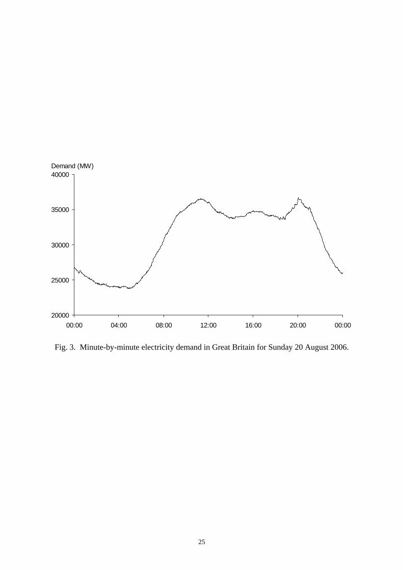
Fig. 3 shows a plot of the series for the first day of the 10-week post-sample period.

We present this plot to emphasise how very much longer the intraday seasonal cycle is than

the very short lead times, which are the main focus in this paper. This suggests that it may be

sufficient, or even preferable, to use a method that makes no attempt to model the intraday

and intraweek seasonal cycles, but instead relies on an extrapolation of the local features of

the series.

3. Univariate Forecasting Methods

In this section, we first present methods that make no attempt to capture the seasonal

features of the data. We then describe methods that model just the intraweek seasonal cycle.

Finally, we present three methods that model both the intraday and intraweek seasonal cycles.

3.1. Non-seasonal Methods

We implemented the following three non-seasonal exponential smoothing methods:

simple, Holt’s (additive trend), and damped Holt’s (damped additive trend) (see Gardner,

2006). We derived parameter values for all methods by the common procedure of minimising

the sum of squared in-sample one-step-ahead forecast errors, with parameters constrained to

lie between zero and one. We used simple averages of the first 30 observations to calculate

initial values for the smoothed components. In all exponential smoothing methods considered

in this study, observations occurring on special days were not used to update the level, trend

or seasonal terms.

As a simplistic benchmark, we produced random walk forecasts. These use the value

of the demand at the forecast origin as the forecast for all future periods. For the simple

6

exponential smoothing method, we derived a value of one for the optimised parameter, which

implied that the forecasts were identical to those from the random walk method. We found

that the damped Holt’s method was similar but slightly more accurate than the Holt’s method

at all lead times, and so in Section 5 we omit the results for the Holt’s method.

3.2. Methods for Single Seasonality

It could be argued that, if the intraweek cycle is modelled well, there is no need for

additional terms to capture the intraday cycle. In view of this, we also considered methods

that only model the intraweek seasonal cycle. We implemented a seasonal version of the

random walk, which takes as a forecast the observed value for the corresponding period in the

previous week. We also implemented the standard Holt-Winters exponential smoothing

method with no trend term and just the intraweek seasonal cycle. We included the adjustment

for first-order autocorrelation used in the double seasonal version of the method described in

the next section. As in the study of Taylor (2003), this adjustment substantially improved the

performance of the standard Holt-Winters method.

3.3. Holt-Winters Exponential Smoothing Adapted for Double Seasonality

The seasonal Holt-Winters exponential smoothing method has been adapted in order

to accommodate the two seasonal cycles in electricity load series (Taylor, 2003). The additive

formulation for minute-by-minute data is given in the following expressions:

1100801440 )1()( −−− −+−−= ttttt lwdyl αα (1) 144010080 )1()( −− −+−−= ttttt dwlyd δδ (2)

100801440 )1()( −− −+−−= ttttt wdlyw ωω (3) ( )1008014401 −−− ++−= ttttt wdlye (4)

tk

ktkttt ewdlky φ+++= +−+− 100801440)(ˆ (5)

where yt is the load in period t; lt is the smoothed level; dt is the seasonal index for the

intraday seasonal cycle; wt is defined as the seasonal index for the intraweek seasonal cycle

7

that remains after the intraday cycle is removed; α, δ and ω are the smoothing parameters;

and )(ˆ kyt is the k step-ahead forecast made from forecast origin t (where k ≤ 1,440). The

term involving the parameter φ, in the forecast function (5), is an adjustment for first-order

autocorrelation in the errors, et. We also considered the multiplicative seasonality formulation

for the method, but this led to very similar post-sample results.

The initial smoothed values for the level and seasonal components are estimated by

averaging the early observations (see Taylor, 2003). We constrained the parameters to lie

between zero and one, and estimated them in a single procedure by minimizing the sum of

squared in-sample forecast errors. Although exponential smoothing parameters tend to be

estimated using one step-ahead in-sample forecast errors, in Section 5, we explain that

interesting results were produced using 10, 20 and 30 minute-ahead errors. The resultant

parameters are shown in Table 1. As in the work of Taylor and McSharry (2007), the value of

φ is very high and the value of α is very low indicating that the adjustment for first-order

autocorrelation has, to a large degree, made redundant the smoothing equation for the level.

This issue is the focus of ongoing research. Building on the work of Hyndman et al. (2002),

the exponential smoothing formulation of expressions (1) to (5) can be written as a single

source of error state space model. This is useful because the model can be used as the basis

for producing prediction intervals and density forecasts (Hyndman et al., 2005).

---------- Table 1 ----------

3.4. Intraday Cycle Exponential Smoothing Model for Double Seasonality

The double seasonal Holt-Winters method of Section 3.3 assumes that the intraday

cycle is the same for all days of the week, and that updates to the smoothed intraday cycle are

made at the same rate for each day of the week. Gould et al. (2007) present an alternative

form of exponential smoothing for intraday data, which allows the intraday cycle for the

8

different days to be represented by different seasonal components. A second notable feature

of their formulation is that it allows the different seasonal components to be updated at

different rates by using different smoothing parameters.

In their empirical study, Gould et al. consider two formulations. The first assumes a

common intraday cycle for the weekdays and a separate common cycle for Saturdays and

Sundays. Their second formulation allows a different intraday cycle for each of the seven

days of the week. The need to select subjectively the number and categorisation of the

intraday cycles is an inconvenience of the method. For their data, the first of their two

formulations produced superior results. However, the use of a common intraday cycle for

Saturdays and Sundays seemed to us unappealing, so in our implementation of the method,

we used the same intraday cycle for the five weekdays and a different intraday cycle for

Saturdays and another for Sundays. The days of the week are thus divided into three types:

weekdays, Saturdays and Sundays. By contrast with Taylor’s double seasonal Holt-Winters,

the Gould et al. method does not involve a representation for the intraweek seasonal cycle.

We term their method ‘intraday cycle exponential smoothing’ due to its focus on intraday

cycles. In period t, the latest estimated values of the three distinct intraday cycles are

expressed as c1t, c2t and c3t, respectively. Three corresponding dummy variables, x1t, x2t and

x3t, are defined as follows:

⎩⎨⎧

=otherwise0

typeofdayainoccursperiodtimeif1 jtx jt

The model is then presented by Gould et al. in state space form as:

ti

tiittt cxly ε++= ∑=

−−

3

11440,1 (6)

ttt ll αε+= −1 (7)

( )3,2,13

1, 1

=⎟⎟⎠

⎞⎜⎜⎝

⎛+= ∑

=− ixcc t

jjtijstiit εγ (8)

9

where lt is the smoothed level; εt is a white noise error term; and α and the γij are the

smoothing parameters. (Rewriting expressions (7) and (8) as recursive expressions delivers a

formulation perhaps more easily recognisable as a form of exponential smoothing.) We used

very similar procedures that we had employed for the double seasonal Holt-Winters method to

initialise the level and seasonal components, and to estimate the model parameters. As with

the double seasonal Holt-Winters method, we considered parameter estimation based on in-

sample forecast errors from a variety of lead times. Our empirical results showed that the

forecasting performance of the method was substantially improved by the inclusion of the

adjustment for first-order autocorrelation that was used in the double seasonal Holt-Winters

method. In Section 5, we present only the results for this form of the Gould et al. method.

The γij can be viewed as a 3×3 matrix of parameters that enables the three types of

intraday cycle to be updated at different rates. The off-diagonal elements of the matrix enable

the intraday cycle of type i to be updated even when the current period is not in a day of type

i. Gould et al. propose a number of restrictions that could be imposed on the matrix of γij

parameters. We included in our study two forms of the method. The first involved estimation

of the matrix of γij parameters with the only restriction being that the parameters lie between

zero and one. The second version of the method involved the additional restrictions of

common diagonal elements and common off-diagonal elements. Interestingly, Gould et al.

note that these additional constraints lead to the method being identical to the double seasonal

Holt-Winters method of expressions (1) to (5), provided seven distinct intraday cycles are

used, instead of three, as in our study. In our discussion of the post-sample forecasting results

in Section 5, we refer to this second form of the model as the restricted form.

10

3.5. ARMA Modelling for Double Seasonality

ARMA models are often used as benchmarks in load forecasting studies (e.g. Laing

and Smith, 1987; Liu et al., 1996; Darbellay and Slama, 2000; Weron, 2006). For intraday

data, a suitable model is the multiplicative double seasonal ARMA model. This model can be

written for minute-by-minute data as

( ) ( ) ( )( ) ( ) ( ) ( ) tQQqtPPp LLLcyLLL εθφ 1008014401008014402121

ΨΘ=−ΩΦ

where c is a constant term; L is the lag operator; εt is a white noise error term; φp, 1PΦ , 2PΩ ,

θq, 1QΘ and 2QΨ are polynomial functions of orders p, P1, P2, q, Q1 and Q2, respectively. The

model is estimated using maximum likelihood based on the standard Gaussian assumption.

In their study of half-hourly data, Laing and Smith (1987) write that forecasting

performance is relatively insensitive to the order of the lag polynomials, and polynomials of

order greater than two are rarely necessary. In other studies of half-hourly load data,

Darbellay and Slama (2000) only use polynomials of order one, while Taylor et al. (2006)

allow polynomials up to order three. In this study of minute-by-minute data, we first

estimated a model with polynomials of order three, but we found all parameters to be

significant (at the 5% significance level), so we increased the order to five, which implied 31

parameters. We again found all parameters to be significant, and, in terms of post-sample

forecasting performance, this model slightly outperformed the model with order three

polynomials. In Fig. 4, we present the plot of the residual autocorrelation for the model with

polynomial of order five. (The acceptance region in the figure is based on the standard error

calculated as the inverse of the square root of the number of residuals at each lag.) The

relatively small autocorrelation values indicate that the model has accommodated much of the

autocorrelation in the demand series. However, for approximately 11% of the lags, the

autocorrelation values are significant at the 5% level. For reasons of parsimony, we deferred

from considering higher order models. We investigated differencing, but this led to poorer

11

forecast accuracy. In Section 5, the seasonal ARMA results correspond to the rather highly

parameterised model with polynomials of order five.

---------- Fig. 4 ----------

In the load forecasting study of Soares and Medeiros (2008), a separate model is fitted

for each hour of the day. Each hourly model consists of a deterministic component and a

seasonal ARIMA component. Fitting a separate model for each hour of the day reduces the

forecasting problem by eliminating the need to model the intraday seasonal cycle. The focus

of Soares and Medeiros is lead times of one day to one week ahead. For much shorter lead

times, the use of separate models for each hour of the day is far less appealing because the

approach does not capture the level of the load at, or just prior to, the forecast origin.

4. A Weather-Based Forecasting Approach

In our study, we implemented the load forecasting approach, based on weather forecasts,

that is currently used at National Grid, which is the transmission company in Great Britain. The

company has used the method for a variety of lead times, including very short-term prediction.

The approach uses weather-based regression models estimated independently for 10 or 11

chosen points on the daily demand curve. The structure of the models is described by Taylor

and Buizza (2003). The chosen points are known as cardinal points and they are either turning

points, such as the evening peak, or strategically chosen fixed points, such as midday or

midnight. Demand forecasts from the weather-based regression models are updated six times

each day in response to the arrival of updated weather predictions. Forecasts of demand for the

minutes between cardinal points are derived from the cardinal point forecasts by a heuristic

interpolation procedure called profiling, which involves fitting a curve to the cardinal points. In

the approach, the forecast origin is treated as the first cardinal point. Baker (1985) describes

how the procedure evolved from the days when computational power limited cost optimisation

to particular critical periods of the day, the cardinal points.

12

The profiling heuristic proceeds by judgementally selecting a past load curve which is

likely to be similar to the load profile for the next day. This is known as the base curve. A

record had not been made of the base curves selected for the 30-week period considered in

our study, and so, in our implementation of the approach, for simplicity, we used the same

weekday of the previous week, which is a common choice for the base curve. The base curve

is fitted to the cardinal points by first calculating the ratio of forecast to base curve demand

for each cardinal point. These are termed the scaling ratios. Scaling ratios for the minutes

between two cardinal points are then calculated by linear interpolation of the scaling ratios at

the two cardinal points. Demand forecasts are then calculated from the product of the base

curve’s demand and the scaling ratio for each minute. The resultant forecast curve will generally

have cardinal points at different periods to the base curve. To reduce this effect, we ran the

profiling procedure three times with the most recent forecast curve as base curve.

Weron (2006) writes that a judgementally selected ‘similar’ past day is sometimes

used as a simple benchmark forecast for a future day. The profiling heuristic, and its use with

weather-based cardinal point forecasts, can be viewed as a development of this idea. Taylor

and Majithia (2000) illustrate how the profiling heuristic is superior to more obvious

interpolation procedures, such as the use of cubic splines. They also consider a number of

potential improvements, including the use of more than one past daily profile in the heuristic

procedure. A development, currently under consideration at National Grid, is the use of fixed

cardinal points located at each half-hour of the day, with the cardinal point forecasts produced

by an independently estimated regression model for each half-hour of the day. This is similar to

the approach of Ramanathan et al. (1997), who produced hourly forecasts by using separate

weather-based models for each hour of the day. Cottet and Smith (2003) and Dordonnat et al.

(2008) develop this approach by accommodating the dependencies between the hourly loads

and estimating simultaneously the equations for each hour of the day.

13

5. Results for Very Short-Term Prediction

In Fig. 5, we present the post-sample mean absolute percentage error (MAPE) for the

methods described in Sections 3 and 4. We also evaluated the root mean squared percentage

error, mean absolute error and root mean squared error, but we do not report these results here

because the ranking of the methods for these measures were very similar to those for the MAPE.

Although the main focus of this study is prediction from 10 to 30 minutes ahead, for

completeness, the figure shows the results for one to 30 minutes ahead. For prediction beyond a

couple of minutes ahead, the accuracy was poor for the non-seasonal univariate methods, and

this is shown in the figure by the results for the random walk method, and simple and damped

Holt’s exponential smoothing. The seasonal random walk method also performed poorly. For all

30 lead times, this method delivered MAPE values of about 2%, and so, given our choice of

scaling of the axes, the results do not appear in the two figures.

---------- Fig. 5 ----------

Turning to the more sophisticated seasonal univariate methods, the figure shows that the

standard Holt-Winters method, implemented to capture the intraweek seasonal cycle, compared

well with the unrestricted intraday cycle exponential smoothing method and with the seasonal

ARMA model. However, the standard Holt-Winters method was outperformed by the double

seasonal adaptation of the Holt-Winters method. Our results for the intraday cycle exponential

smoothing method show that the restricted version of the method was more accurate than the

unrestricted version, and this is consistent with the findings of Taylor and McSharry (2007) for

forecasting longer lead times based on half-hourly data. By contrast with the results of Taylor

and McSharry, for our minute-by-minute data, the intraday cycle exponential smoothing method

slightly outperformed the double seasonal Holt-Winters method when each was estimated using

one-step ahead in-sample forecast errors.

In view of our focus on lead times between 10 and 30 minutes ahead, for the restricted

intraday cycle method and the double seasonal Holt-Winters method, we experimented with

14

parameter estimation based on 10, 20 and 30 minute-ahead in-sample forecast errors. For both

methods, this delivered noticeable improvement in forecast accuracy for lead times beyond one

minute ahead. Interestingly, it also resulted in a reverse in the rankings of the two methods, and

this is shown in Fig. 5 where we plot the results for the methods with parameters estimated using

30 minute-ahead prediction.

Fig. 5 shows that the weather-based forecasting approach was not competitive, although

the ranking of the method improves as the lead time increases. This was, perhaps, to be expected,

as the method was designed at National Grid for lead times of several hours ahead and longer.

Indeed, as we discussed briefly in Section 1, the usefulness of weather forecasts is more obvious

for lead times longer than 30 minutes ahead.

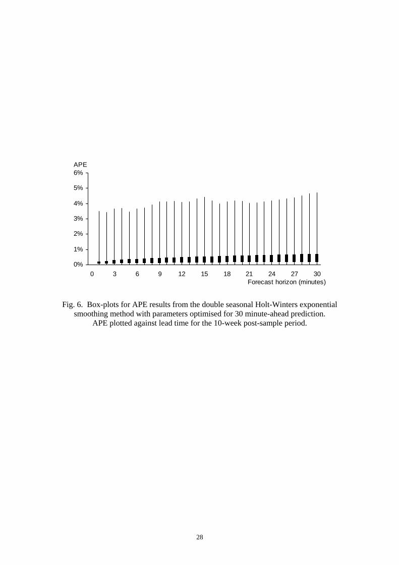
In Figs. 6 and 7, we present box-plots for the APE results from the two best performing

methods in Fig. 5: the double seasonal Holt-Winters exponential smoothing method and the

restricted intraday cycle exponential smoothing method with parameters for both methods

optimised for 30 minute-ahead prediction. The one noticeable difference between the two box-

plots is that the maximum APE for each lead time is noticeably smaller for the double seasonal

Holt-Winters method.

---------- Figs. 6, 7 and 8 ----------

In Fig. 8, we plot the MAPE results for 20 minute-ahead prediction, against the time of

day of the forecast period, for the two best performing methods in Fig. 5. Understandably, the

larger MAPE values in Fig. 8 tend to correspond to the periods of the day when demand is

changing the most. The restricted intraday cycle method seems to perform better between about

05:00 and 08:00, while the double seasonal Holt-Winters adaptation is more accurate between

about 18:00 and 23:00. An interesting feature of Fig. 8 is the very large MAPE values for the

early periods of the day for the intraday cycle exponential smoothing method. For this method,

the same feature was present in similar plots for different lead times, and for the method with

parameters estimated using forecast errors from other lead times. The poor predictions for the

15

early periods of the day would seem to be due to the method’s use of three separate types of

intraday cycles. Connecting the separate intraday cycles leads to a discontinuity at midnight. For

k period-ahead prediction, this sizeable error is only fed back to the model after k periods,

resulting in sizeable error for the first k periods of the day. This is evident in Fig. 8, which has

large 20 minute-ahead MAPE values for the intraday cycle exponential smoothing method for

the first 20 minutes of the day.

6. Results for Prediction Beyond the Very Short-Term

Having established the usefulness of the double seasonal Holt-Winters method for

very short-term prediction, we were curious to establish how the method would perform for

prediction beyond 30 minutes ahead. Since the method performed particularly well, in Section

5, when the parameters were estimated using 30 minute-ahead in-sample forecast errors, a

first issue to consider was how this version of the method, applied to minute-by-minute data,

would compare with the method applied to half-hourly data, which has been the focus of

previous studies (e.g. Taylor, 2003). We were unsure as to whether the method applied to

higher frequency data would have an advantage or disadvantage. As it turned out, we found

that these two versions of the method performed very similarly for prediction from 30 minutes

ahead to a day ahead. However, this comparison seemed a little unsatisfactory because the

method based on half-hourly data could only be evaluated for data at this same frequency, and

thus we were not using all of the minute-by-minute time series for the evaluation. Indeed, an

inherent weakness of a method, built on half-hourly data, is that it is unable to produce

predictions for minutes between the half-hours or to produce forecasts from forecast origins

between the half-hours. In view of this, the method applied to minute-by-minute data, with

parameters estimated using 30 minute-ahead forecast errors, has the appeal of flexibility with

seemingly no loss of accuracy.

16

We next turned our attention to the common assumption that a method based on weather

forecasts will outperform a univariate method for prediction beyond a few hours ahead. We are

not aware of any consensus in the literature as to the length of the lead time beyond which a

weather-based method will be better. Indeed, there have been no studies comparing the double

seasonal Holt-Winters method with a weather-based forecasting approach. In Fig. 9, we plot

MAPE values for the 1,440 lead times from one minute ahead to one day ahead. The figure

compares the performance of the company’s weather-based method, described in Section 4, and

the intraday cycle and double seasonal Holt-Winters methods. For both the exponential

smoothing methods, parameters were estimated using 30 minute-ahead in-sample forecast errors.

In view of the results of Section 5, it is not surprising to see that, the double seasonal Holt-

Winters method outperforms the intraday cycle exponential smoothing method. Comparing the

double seasonal Holt-Winters method with the weather-based approach, we see that the

univariate method is outperformed beyond about four hours ahead. Our final experiment

involved using a simple average of the weather-based approach and the double seasonal Holt-

Winters method with parameters estimated using 30 minute-ahead in-sample forecast errors.

Combining forecasts has been shown to lead to an improvement in accuracy in many different

applications. Recent examples in the area of energy forecasting are the studies of Jursa and

Rohrig (2008) and Sánchez (2008). A combination of forecasts has particular appeal when the

different methods are based on different information sources. This is the case in our study where

we have a weather-based method and a univariate method. As shown in Fig. 9, the combination

achieved the best performance beyond about an hour ahead.

---------- Fig. 9 ----------

7. Summary and Conclusions

In this paper, our main focus has been to use a time series of minute-by-minute British

electricity demand to evaluate a variety of forecasting methods for lead times between 10 and

17

30 minutes. For such very short lead times, we found the most accurate method to be the

double seasonal adaptation of the Holt-Winters exponential smoothing method. This result is

consistent with the findings of previous studies that have looked at longer lead times based on

hourly and half-hourly data. The new intraday cycle exponential smoothing method also

performed well, but the double seasonal Holt-Winters method produced the best results when

parameters were estimated using 30 minute-ahead in-sample forecast errors. Our study also

provided insight for the choice between univariate and multivariate methods because,

included in our study, was a regression-based method using weather forecasts as input. This

method was not competitive for very short-term prediction.

The results for prediction beyond 30 minutes ahead showed that the weather-based

approach was superior for lead times longer than about four hours. However, combining this

method with the double seasonal Holt-Winters method led to the best results beyond about

one hour ahead. This suggests that the double seasonal Holt-Winters method should be used

for very short-term prediction, and that it can be used within a combined forecast to improve

the accuracy of the weather-based method for longer lead times.

It is perhaps surprising that the weather-based method, within a combination, is able to

improve a univariate method for lead times as short as one hour. However, it is worth bearing

in mind that the weather-based method does not simply involve weather-based regression

models. It also involves the rather unusual profiling heuristic, and this married with the

weather-based cardinal point forecasts does seem to provide useful additional information for

prediction at lead times beyond about an hour ahead. Another perhaps surprising result was

the degree to which the combination was more accurate than the weather-based method for

the longer lead times. We offer two explanations for this. First, the weather-based method

uses regression models that capture little of the time series properties of the load series.

Although there is substantial useful judgemental adjustment made to the cardinal point

forecasts, it is not too surprising that this judgement is not sufficient to capture the complex

18

autocorrelation structure in the load time series. A second explanation is that our

implementation of the weather-based approach involved a simplified version of the profiling

heuristic. As we explained in Section 4, we used the same day of the week from the previous

week as base curve, while in reality the National Grid forecasters judgementally select a

suitable past load profile. Our implementation lacked this useful judgemental input. Having

said that, it is an obvious advantage of the univariate methods that they require minimal

judgemental input. This, coupled with the fact that they do not rely on weather forecasts,

gives the univariate methods strong appeal, in terms robustness, for online load prediction.

The success of the two exponential smoothing methods, designed specifically for

intraday data, motivates research into a new method that is able to capture the appealing

features of both. This is the focus of our current work. In future work, it would be interesting

to explore further the potential for combining forecasts. It may be that other combining

methods can deliver improved accuracy. An alternative to combining is to switch between

methods, and this proposal is, to some degree, supported by the results of Fig. 8, which show

a different method performing better at different times of the day.

It would be interesting to see a comparison of the methods considered in this paper for

other load time series and for a sample of data taken from a different period of the year. A

further issue of interest is the length of the time series used to estimate the methods. We do

not claim in the paper that our results provide conclusions for all electricity demand datasets,

so it is clearly necessary for practitioners to perform similar experimentation for their data. In

our current work, we are investigating the benefit of using several years of intraday load data

to estimate univariate methods. The availability of such data motivates the adaptation of the

double seasonal methods in order to accommodate the annual seasonal cycle.

19

Acknowledgements

We are grateful to Matthew Roberts of National Grid for supplying the data and

information regarding the very short-term forecasting context at the company. We are also

grateful for the helpful comments of the editor, Toni Espasa, and two anonymous referees.

References

Alves da Silva, A. P., Ferreira, V.H. & Velasquez, R.M.G. (2008). Input space to neural

network based load forecasting, International Journal of Forecasting, forthcoming.

Baker, A.B. (1985). Load forecasting for scheduling generation on a large interconnected

system. In: Bunn, D.W. & Farmer E.D. (eds). Comparative Models for Electrical Load

Forecasting. New York: Wiley, 57-67.

Cancelo, J. R., Espasa, A., & Grafe, R. (2008). Forecasting from one day to one week ahead

for the Spanish system operator, International Journal of Forecasting, forthcoming.

Charytoniuk, W. & Chen, M.-S. (2000). Very short-term load forecasting using artificial

neural networks, IEEE Transactions on Power Systems, 15, 263-268.

Cottet, R. & Smith, M. (2003). Bayesian modeling and forecasting of intraday electricity load,

Journal of the American Statistical Association, 98, 839–849.

Darbellay, G.A. & Slama, M. (2000). Forecasting the short-term demand for electricity – Do

neural networks stand a better chance?, International Journal of Forecasting, 16, 71-83.

Dordonnat, V., Koopman, S. J., Ooms, M., Dessertaine, A., & Collet, J. (2008). An hourly

periodic state space model for modelling French national electricity load, International

Journal of Forecasting, forthcoming.

Gardner, E.S., Jr. (2006). Exponential smoothing: the state of the art - Part II, International

Journal of Forecasting, 22 637-666.

20

Gould, P.G., Koehler, A.B., Vahid-Araghi, F., Snyder, R.D., Ord, J.K. & Hyndman, R.J.

(2007). Forecasting time-series with multiple seasonal patterns, European Journal of

Operational Research, forthcoming.

Hippert, H.S., Pedreira, C.E. & Souza, R.C. (2001). Neural networks for short-term load

forecasting: a review and evaluation, IEEE Transactions on Power Systems, 16, 44-55.

Hyndman, R.J., Koehler, A.B., Snyder, R.D. & Grose, S. (2002). A state space framework for

automatic forecasting using exponential smoothing methods, International Journal of

Forecasting, 18, 439-454.

Hyndman, R.J., Koehler, A.B., Ord, J.K. & Snyder, R.D. (2005). Prediction intervals for

exponential smoothing using two new classes of state space models, Journal of Forecasting,

24, 17-37.

Jursa, R. & Rohrig, K. (2008). Short-term wind power forecasting using evolutionary

algorithms for the specification of artificial intelligence models, International Journal of

Forecasting, forthcoming.

Laing, W.D. & Smith, D.G.C. (1987). A comparison of time series forecasting methods for

predicting the CEGB demand. Proceedings of the Ninth Power Systems Computation

Conference.

Liu, K., Subbarayan, S., Shoults, R.R., Manry, M.T., Kwan, C., Lewis, F.L. & Naccarino, J.

(1996). Comparison of very short-term load forecasting techniques, IEEE Transactions on

Power Systems, 11, 877-882.

Ramanathan, R., Engle, R., Granger, C.W.J., Vahid-Araghi, F. & Brace C. (1997). Short-run

forecasts of electricity loads and peaks, International Journal of Forecasting, 13, 161-174.

Medeiros, M.C. & Soares, L.J. (2008). Modeling and forecasting short-term electricity load:

A comparison of methods with an application to Brazilian data, International Journal of

Forecasting, forthcoming.

21

Sánchez, I. (2008). Adaptive combination of forecasts with application to wind energy,

International Journal of Forecasting, forthcoming.

Taylor, J.W. (2003). Short-term electricity demand forecasting using double seasonal

exponential smoothing, Journal of Operational Research Society, 54, 799-805.

Taylor, J.W. & Buizza R. (2003). Using weather ensemble predictions in electricity demand

forecasting, International Journal of Forecasting, 19, 57-70.

Taylor, J.W., M. de Menezes, L.M. & McSharry, P.E. (2006). A comparison of univariate

methods for forecasting electricity demand up to a day ahead, International Journal of

Forecasting, 22, 1-16.

Taylor, J.W. & Majithia, S. (2000). Using combined forecasts with changing weights for

electricity demand profiling, Journal of the Operational Research Society, 51, 72-82.

Taylor, J.W. & McSharry, P.E. (2007). Short-term load forecasting: An evaluation based on

European data, IEEE Transactions on Power Systems, 22, 2213-2219.

Trudnowski, D.J., McReynolds, W.L. & Johnson, J.M. (2001). Real-time very short-term load

prediction for power-system automatic generation control, IEEE Transactions on Control

Systems Technology, 9, 254-260.

Weron, R. (2006). Modelling and Forecasting Electric Loads and Prices. Chichester: Wiley.

22

Table 1. Parameters for the double seasonal Holt-Winters method of expressions (1) to (5), estimated using in-sample forecast errors from different lead times.

Lead time of errors used in parameter estimation α δ ω φ

1 0.001 0.031 0.156 0.996

10 0.001 0.171 0.170 0.997

20 0.001 0.231 0.179 0.998

30 0.001 0.265 0.190 0.998

23

15000

20000

25000

30000

35000

40000

45000

50000

55000

02/04/2006 02/05/2006 02/06/2006 02/07/2006 02/08/2006 01/09/2006 02/10/2006

Demand (MW)

Fig. 1. Minute-by-minute electricity demand in Great Britain from Sunday 2 April 2006 to Saturday 28 October 2006.

24

20000

25000

30000

35000

40000

45000

50000

20/0

8/20

06

21/0

8/20

06

22/0

8/20

06

23/0

8/20

06

24/0

8/20

06

25/0

8/20

06

26/0

8/20

06

27/0

8/20

06

28/0

8/20

06

29/0

8/20

06

30/0

8/20

06

31/0

8/20

06

01/0

9/20

06

02/0

9/20

06

03/0

9/20

06

Demand (MW)

Fig. 2. Minute-by-minute electricity demand in Great Britain for Sunday 20 August 2006 to Saturday 2 September 2006.

25

20000

25000

30000

35000

40000

00:00 04:00 08:00 12:00 16:00 20:00 00:00

Demand (MW)

Fig. 3. Minute-by-minute electricity demand in Great Britain for Sunday 20 August 2006.

26

-0.04

-0.03

-0.02

-0.01

0

0.01

0.02

0.03

0.04

0 1440 2880 4320 5760 7200 8640 10080Lag

Fig. 4. Autocorrelation function for the residuals from the seasonal ARMA model. Grey horizontal lines bound 95% acceptance region for test of zero autocorrelation.

27

MAPE (%)

0.1%

0.2%

0.3%

0.4%

0.5%

0.6%

0.7%

0.8%

0 5 10 15 20 25 30Forecast horizon (minutes)

Random Walk and Simple Exp Sm

Damped Holts Exp Sm

Weather-Based

Holt-Winters Exp Sm

Unrestricted Intraday Cycle Exp Sm - Optimised for 1 Min Ahead

Seasonal ARMA

Double Seasonal Holt-Winters Exp Sm - Optimised for 1 Min Ahead

Restricted Intraday Cycle Exp Sm - Optimised for 1 Min Ahead

Restricted Intraday Cycle Exp Sm - Optimised for 30 Min Ahead

Double Seasonal Holt-Winters Exp Sm - Optimised for 30 Min Ahead

Fig. 5. MAPE results plotted against lead time for the 10-week post-sample period for lead times from one to 30 minutes ahead.

28

0%

1%

2%

3%

4%

5%

6%

0 3 6 9 12 15 18 21 24 27 30Forecast horizon (minutes)

APE

Fig. 6. Box-plots for APE results from the double seasonal Holt-Winters exponential smoothing method with parameters optimised for 30 minute-ahead prediction.

APE plotted against lead time for the 10-week post-sample period.

29

0%

1%

2%

3%

4%

5%

6%

0 3 6 9 12 15 18 21 24 27 30Forecast horizon (minutes)

APE

Fig. 7. Box-plots for APE results from the restricted intraday cycle exponential smoothing method with parameters optimised for 30 minute-ahead prediction.

APE plotted against lead time for the 10-week post-sample period.

30

0.0%

0.3%

0.6%

0.9%

1.2%

1.5%

1.8%

00:00 04:00 08:00 12:00 16:00 20:00 00:00Time of day

MAPE (%)

Restricted Intraday Cycle Exp Sm - Optimised for 30 Min Ahead

Double Seasonal Holt-Winters Exp Sm - Optimised for 30 Min Ahead

Fig. 8. MAPE results for 20 minute-ahead prediction, plotted against the time of day of the forecast period, for the 10-week post-sample period.

31

0.0%

0.3%

0.6%

0.9%

1.2%

1.5%

1.8%

0 240 480 720 960 1200 1440Forecast horizon (minutes)

MAPE (%)

Restricted Intraday Cycle Exp Sm - Optimised for 30 Min Ahead

Double Seasonal Holt-Winters Exp Sm - Optimised for 30 Min Ahead

Weather-Based

Combination of Weather-Based and Double Seasonal Holt-Winters Exp Sm

Fig. 9. MAPE results plotted against lead time for the 10-week post-sample period for lead times from one minute to one day ahead.