An Experimental Evaluation of Tax Evasionand Tax Enforcement in Denmark∗

Henrik Jacobsen Kleven, London School of Economics

Martin Knudsen, Danish Inland Revenue (SKAT)

Claus Thustrup Kreiner, University of Copenhagen

Søren Pedersen, Danish Inland Revenue (SKAT)

Emmanuel Saez, UC Berkeley

Preliminary Working Draft: March 2008

Abstract

This paper analyzes a randomized evaluation of tax enforcement and tax evasion carriedout in collaboration with Danish Inland Revenue (SKAT). In the base year, a stratifiedand representative sample of over 40,000 Danish individual tax filers was selected for theexeriment. Half of those tax filers were randomly selected to be thoroughly audited, whilethe rest were deliberately not audited. The following year, “threat-of-audit” letters wererandomly assigned and sent to those tax filers. This experiment allows us to study incometax compliance in Denmark in great detail, as well as the causal effects of (a) prior auditsand (b) audit probability on subsequent reporting behavior. We find that tax compliancein Denmark is high overall, but that there is substantial tax evasion on purely self-reportedincome, i.e. income which is not subject to double reporting by third parties. This suggestthat the informational framework is more important than social or psychological effects inexplaining tax compliance. We find that threat-of-audit letters have significant effects on self-reported income adjustments, and that these effects are larger for tax filers not audited in theprevious year. Letters also increase the likelihood of downward adjustments (which reducetax liability), which can be explained by taxpayers trading off the cost of filing correctlyagainst the cost of having to deal with tax examiners. Prior audits also significantly increasethe likelihood of self-reporting higher incomes the following year, implying that individualsupdate their beliefs about audit probability based on experiencing an audit.

∗We are grateful to Jakob Egholt Søgaard for outstanding research assistance. We thank Oriana Bandiera,Richard Blundell, Monica Singhal, Joel Slemrod, and numerous seminar participants for comments and discus-sions. Financial support from ESRC Grant RES-000-22-3241, NSF Grant SES-0850631, and a grant from theEconomic Policy Research Network (EPRN) is gratefully acknowledged. The responsibility for all interpretationsand conclusions expressed in this paper lie solely with the authors and do not necessarily represent the views ofthe Danish tax administration (SKAT) or the Danish government.

1 Introduction

Most of the public finance literature studies the effects and design of tax policy assuming that

taxpayers always comply with the tax law and that any given tax system can be enforced at no

cost. In reality, the design of tax enforcement policies that limit tax evasion is central to ensure

that a tax system is non-capricious, efficient, and fair. The economic theory of crime as ap-

plied to tax evasion emphasizes the probability of being detected and the severity of punishment

upon detection as the key deterrents to noncompliance. Tax practitioners would additionally

emphasize the key role of information reporting from third parties and withholding at source

as important aspects of effective tax enforcement. To make informed decisions about the de-

sign of tax enforcement policies, we need empirical knowledge of the link between evasion and

enforcement efforts such as audit strategies, penalties, and information collection processes.

There is a voluminous literature estimating the effects of tax enforcement on evasion using

observational and non-experimental data.1 This literature faces a number of difficult challenges

with regard to measurement and identification. One obvious problem is that the dependent vari-

able is not observed accurately, because tax evasion by its nature is something that taxpayers are

unwilling to reveal truthfully when asked. Second, the independent variables–audit probabili-

ties, actual audits, and penalties–are very difficult to capture at the individual level, because

information about audit strategies is confidential and typically inaccessible to researchers. Third,

the variation in enforcement parameters is not exogenous but rather an endogenous response

to compliance itself. This requires the use of instrumental variables, but credible instruments

are very hard to come by in this area and the results turn out to be often sensitive to the

empirical specification. These generic problems motivate adopting an experimental approach to

estimating tax evasion.

This paper presents new evidence on tax audits and tax evasion based on a large randomized

field experiment carried out in collaboration with the Danish tax collection agency (SKAT).2

The experiment imposes different audit regimes on randomly selected taxpayers, and has been

designed to inform us about the effects of audit probabilities and prior audits on tax evasion as

well as the total extent of non-compliance. SKAT has given us access to virtually all tax and

1Excellent surveys of this literature are provided by Andreoni et al. (1998) and Slemrod and Yitzhaki (2002).2The Danish word SKAT translates to TAX.

1

audit data matched to very rich socio-economic administrative data sets at Statistics Denmark.3

The extraordinary degree of cooperation and data access presents a unique opportunity to learn

about the effects and design of enforcement policies.

The experiment was implemented in two stages during the filing and auditing seasons of 2007

and 2008 (corresponding to incomes earned in 2006 and 2007 respectively). In the first stage, a

stratified random sample of about 26,000 taxpayers (employees, self-employed, and corporations)

was selected by SKAT for audits of the tax returns they had just filed in 2007. These tax audits

were comprehensive in the sense that every item on the return was examined, and the audits

used up 21% of all resources devoted to tax audits in 2007. In the case of detected misreporting,

the tax liability was corrected and taxpayers were penalized depending on the nature of the error

and as appropriate according to Danish law. Taxpayers were not told that the audits were part

of a special study. To evaluate the effects of audits on future reporting, a mirror random sample

of 26,000 taxpayers was selected and assigned to a no-audit group. No taxpayer in this group

was audited even if the characteristics of the return would normally have triggered an audit.

In the second stage, employees (but not self-employed and corporations) in the full-audit

and the no-audit groups were randomly assigned to three subgroups equal to 1/3 the size of

the original group. In one group, taxpayers received letters from SKAT in April 2008 telling

them that the returns they were about to file would be audited. In a second group, taxpayers

were told that half of the filers in their group would be audited, while a third group received

no letter. The second stage therefore provides exogenous variation in the probability of being

audited, conditional on having been audited the prior-year in the first stage or not. The audit

probability is 100% for the first group, 50% for the second group, and equal to the current

perceived probability in the third group. The current audit rate in Denmark (= 4.2%) suggests

that perceived probabilities in the third group are low on average.

In this paper, we present findings for individual tax filers (employees and the self-employed)

and report four sets of results. The first set of results show the misreporting uncovered by tax

inspectors in the full-audit group. We find that the overall tax evasion uncovered by audits is

modest: about 1.7% of total reported income. But underneath the average amount of detected

underreporting, there is considerable heterogeneity across different income sources and across

3The data extracts are prepared within SKAT and stripped of all individual identifiers before the analysis.Furthermore, SKAT makes a final check on the statistical output presented in the paper to ensure that noconfidential information is disclosed.

2

different taxpayers. As for income source, we demonstrate that the key distinction is whether

the income item is subject to information reporting from third parties such as employers, banks,

and pension funds, or whether the income item is purely self-reported. For self-reported items,

tax evasion is about 12%, whereas tax evasion is virtually nil for third-party reported items. As

for heterogeneity across taxpayers, we find that underreporting is much higher for individuals

identified as likely evaders by the computer-generated audit flag system used by SKAT as part

of their regular audit procedure. We also find that evasion is more prevalent among taxpayers

with negative income, taxpayers at the top of the income distribution, the self-employed, and

males.

The second set of results pertain to the effect of the audit probability on reported income by

comparing the threat-of-audit letter and no-letter groups. We focus on the effect on self-reported

income as measured by the difference between the filed return and a pre-populated return con-

taining third-party information.4 We find that individuals receiving a threat-of-audit letter were

more likely to adjust the pre-populated return, either upwards by self-reporting additional in-

come or downwards by claiming additional deductions and losses. Although taxpayers respond

in both directions, the effect on upward adjustments is much stronger than on downward ad-

justments. The upward adjustments are consistent with standard theories of tax evasion, while

we suggest an explanation for the downward adjustments based on taxpayers trading off the

cost of filing correctly against the cost of having to deal with tax examiners. We also find that

the letter effect is stronger for those who were not audited in the first stage, suggesting that

taxpayers were initially overstating the cost of being audited and that audited taxpayers have

subsequently adjusted their perceptions of the consequences of an audit.

The third set of results show the effect of experiencing an audit on income in the following

year. Audits may affect future reported income to the extent that they lead taxpayers to adjust

their perceptions of the probability of being audited and/or if they learn something about the

consequences of an audit such as the capability of tax auditors to detect cheating, the severity

of penalties, and the hassle and aggravation associated with the auditing process. We find that

the effect of audits on the likelihood of making self-reported adjustments to the pre-populated

4 In principle, a threat of audit may also affect third parties who are contemplating a collusion with a taxpayerto evade tax. However, in this experiment, the threat-of-audit letters were sent to taxpayers after the deadlinefor information reporting from third parties, implying that third-party reporting was unable to respond to theletter treatment.

3

return and on the likelihood of reporting a higher total income in the following year are both

positive but quite small. Given our previous result suggesting that taxpayers learn than tax

audits are not as bad as they thought, these results indicate that being audited increases the

subjective probability of being audited again.

The fourth set of results is a cost-benefit analysis of different audit strategies. The overall

conclusion is that untargeted audits are fairly close to break even in terms of the revenue they

generate relative to audit costs to the government, while targeted audits are strongly revenue

increasing. The regular audit procedure based on automated flags is successful in targeting

cheaters overall, although there seems to be room for improvement. The flag system is not

good at screening honest and dishonest taxpayers within the group of self-employed, and there

currently seems to be potential over-auditing of the self-employed relative to employees. The

reason for this result is a combination of the poor flag-screening for the self-employed, and the

fact that it is much more costly to audit the self-employed than employees.

An emerging consensus in the literature on tax evasion is that observed compliance in devel-

oped nations is much higher than predicted by both economic theory and laboratory experiments

at realistic levels of audit probabilities and penalties. It has been suggested by many studies

that observed compliance levels can only be explained by accounting for psychological and so-

ciological aspects of the reporting decision such as guilt, shame, and tax morale. While we do

not deny the importance of behavioral aspects in the decision to evade on taxes, the evidence

presented in this paper points to a more classic information story. In particular, although de-

tectable evasion is fairly small overall, tax evasion on purely self-reported income is substantial.

Moreover, we find that both prior audits and especially audit threats have significant deterrence

effects on self-reported income. Our results suggest that compliance is high in developed coun-

tries because of the widespread use of double reporting by the taxpayer and a third party such

as the employer or financial institution. At the end of the paper, we discuss some conceptual

and theoretical reasons for the efficacy of third-party reporting, and set out a future research

agenda to establish a general theory of tax enforcement with third-party reporting.

The paper is organized as follows. Section 2 presents a simple conceptual framework and

reviews the literature. Section 3 describes the Danish income tax context, experimental design,

and data. Sections 4 and 5 present our empirical results and cost-benefit analysis. Section 6

offers concluding remarks and an agenda for future work.

4

2 Conceptual Framework and Prior Work

2.1 Theory

The best-known model of tax evasion is due to Allingham and Sandmo (1972)–henceforth AS–

who applied the economic theory of crime by Becker (1968) to the case of tax evasion. In the

AS-model, a taxpayer’s true income y is not costlessly observed by the tax authorities, and

the taxpayer may therefore decide to evade taxes by reporting income z < y. The tax rate on

income is t, and the government enforces this tax through a system of audits and penalties. The

probability of an audit is p, and it is assumed that all evasion can be detected by an audit.

When audited, the taxpayer is forced to pay the evaded tax plus a penalty, (1 + θ) t (y − z).5

The taxpayer maximizes expected utility

(1− p) · u (y − tz) + p · u (y − tz − (1 + θ) t (y − z)) . (1)

True income is assumed fixed, so the only choice variable for the taxpayer is how much to report

z. An interior solution with z < y is characterized by

u0 (cA)

u0 (cN)=1− p

pθ, (2)

where cA and cN denote consumption in the audited and non-audited states. From this first-

order condition, it is easy to see that reported income is increasing in the audit probability p and

in the penalty θ. If p and θ are high enough, the taxpayer is pushed to a corner solution with

truthful reporting, z = y. The condition for truthful reporting to be optimal is that, at z = y,

the left-hand side of (2) is greater than or equal to the right-hand side. For our purpose, it is

important to note that this corner condition will always be satisfied when the audit probability

tends to 1, because in this case the right-hand side tends to zero while the left-hand side remains

positive.

The basic AS-model represents a very strong simplification of the real-world reporting and

auditing environment, and it is worthwhile mentioning a few generalizations that will play a role

in our empirical study. First, the AS-model implicitly assumes that all income is subject to self-

reporting, while in practice a substantial part of income is subject to information reporting from

third parties. As long as taxpayers and third parties do not collude to evade taxes, information

5By letting the penalty depend on the understated tax rather than understated income, we are adopting themore realistic Yitzhaki (1974) formulation of the AS-model.

5

reporting provides perfect information over part of taxable income. Therefore, third party

reported income can be considered as a special case with p = 1: if the individual deviates from

the third party report, the government will detect the deviation with probability (almost) one.6

Second, it is not realistic that audits will detect all evasion and taxpayers may realize this. If

income consists of some detectable and some non-detectable items, an audit probability of 1

will push taxpayers to full reporting only on the detectable items. Third, it is not realistic that

taxpayers have perfect information over the enforcement parameters (p and θ) and over what can

be detected by tax inspectors, because tax audits are rare events and because audit strategies are

confidential information. In a more general model, tax audits may affect behavior by changing

perceptions regarding the probability and consequences of an audit. Fourth, real-world tax

codes are complex, and this may lead taxpayers to make honest mistakes and sometimes to

overstate taxable income. Because it is very hard to draw the line between an honest mistake

and deliberate fraud, using the penalty instrument is seriously constrained. Fifth, the audit

probability is not fixed but a function of the taxpayer report, and this may create a strategic

interaction between the taxpayer and the tax administrator. Sixth, income tax filing is not

a static decision but a repeated annual event. Accounting for dynamic reporting imply that

taxpayers may condition their reports on past reports and past audit experiences.

2.2 Empirical Literature Review

Over the past few decades, a blossoming empirical literature has studied the link between tax

evasion and tax rates, penalties, audit probabilities, prior audit experiences, and socio-economic

characteristics. Most of this literature relies on observational and non-experimental data, which

creates a number of problems with regard to measurement and identification. The first prob-

lem is that the dependent variable–evasion–is not observed accurately, because taxpayers

go to great lengths to conceal their evasion and because tax authorities do not make audit

records publicly available except in aggregate form. The second problem is that the indepen-

dent variables–audits, threat of audits, penalties–are difficult to capture at the individual

level, because enforcement strategies are confidential information and inaccessible to researchers

in most cases. The third problem is that, even where reasonable measures of evasion and its var-

ious determinants have been available (mostly macro-data studies at the district or state level),

6 In practice, tax agencies do indeed systematically match third party reports to self-reports.

6

the variation in tax rates and enforcement efforts is not exogenous but rather an endogenous

response to compliance. This poses an important threat to identification and requires the use

of instrumental variables.7 Andreoni et al. (1998) and Slemrod and Yitzhaki (2002) provide

critical reviews of this literature and argue that none of the available instruments are likely to

satisfy the assumptions for IV-estimation to be consistent.

These generic problems motivate the use of an experimental approach to estimate evasion.

There are three sources of experimental data that have been explored in the literature. The

first source is the Taxpayer Compliance Measurement Program (TCMP) of the Internal Rev-

enue Service in the United States. The household TCMP is a program of thorough tax audits

conducted on a stratified random sample of personal income tax returns approximately every

third year from 1965 to 1988. The TCMP program has provided very useful information re-

garding the extent of evasion and the size of the tax gap, the difference between taxes owed

and taxes paid voluntarily and on a timely basis. Most of the non-experimental studies cited

above have been based on (aggregated) TCMP records. As pointed out in Andreoni, Erard, and

Feinstein (1998) and Bloomquist (2003), various studies based on TCMP data have shown that

under-reporting is much higher for income categories such as business income which have little

third party reporting than income categories such as wages and salaries, which are in general

double reported by a third party (see Klepper and Nagin, 1989; Long and Swingden, 1990;

Christian 1994, Internal Revenue Service, 1996). To our knowledge however, no TCMP based

study has precisely and systematically compared compliance rates with third-reported income

items to self-reported items as we do in this paper. Furthermore, TCMP does not provide useful

exogenous variation in enforcement variables. Because audits are not pre-announced, there is

no variation in the audit probability. Moreover, because audited taxpayers are told that this is

part of a special study and that audit selection is random, TCMP cannot be used to study the

effects of prior audits on reporting.

A second source of experimental data has been generated by laboratory experiments. These

are multi-period reporting games involving participants (mostly students) who receive and re-

port income, pay taxes, and face risks of being audited and penalized. Lab experiments have

consistently shown that penalties, audit probabilities, and prior audits increase compliance (e.g.

7The list of studies using district-level or state-level data on evasion and audit rates, and where an IV-strategywas adopted to control for the endogenoeity of the audit rate, include Dubin and Wilde (1988), Beron et al.(1992), Dubin et al. (1990), and Pommerehne and Frey (1992).

7

Friedland et al., 1978; Becker et al., 1987; Alm et al., 1992a,b, 2008). But Alm et al. (1992a,b)

show that, when penalties and audit probabilities are set at realistic levels, their deterrent effect

is quite small and the laboratory therefore tends to predict more evasion than we observe in

practice. The key problem is that the lab environment by its nature is artificial and therefore

likely to miss important aspects of the real-world reporting environment.

The third source of data concerns a small but unique randomized field experiment involv-

ing about 1700 taxpayers in Minnesota. Like the experiment we consider in this paper, the

Minnesota experiment sent threat-of-audit letters to taxpayers, thereby providing exogenous

variation in the audit probability. This experiment was studied by Slemrod et al. (2001) who

considered the effect of the audit threat on reported income. They found that results are het-

erogeneous with respect to income level and opportunities to evade, and surprisingly that a

higher auditing probability lead to a reduction in reported income at the top of the distribution

(although this effect was not statistically significant).

Our paper is closest in methodology to the important work by Slemrod et al. (2001), but our

study is based on a richer set of treatments and a much larger sample size. Moreover, we have

benefitted from essentially full access to tax and audit records at the Danish tax administration

allowing us to carry out a much more detailed empirical analysis. In the following section, we

describe the Danish income tax, enforcement system, the experimental design, and the data.

3 Context, Experimental Design, and Data

3.1 The Danish Income Tax and Enforcement System

The Danish income tax system is fairly complex. Rather than applying a progressive rate

structure to a single measure of taxable income, it is based a number of different income concepts

that are taxed differently. This system implies, for example, that labor income, capital income,

and deductions are associated with different marginal tax rates, and that the tax rate on capital

depends on whether net capital income is positive or negative. The main income concepts of

the individual income tax system are described in Table 1, while the tax rates and tax brackets

associated with the different income concepts are shown in Table 2. The tax system in these

two descriptive tables apply to all individual tax filers (transfer recipients, employees, and the

self-employed), but there are additional provisions for the self-employed that will be described

8

below.

Taxable labor income includes all types of earnings, and is taxed directly by a proportional

labor market tax equal to 8%. All other taxes on labor income apply to tax bases net of the

labor market tax, implying that the effective tax rate is only 92% of the statutory tax. Personal

income includes labor income plus social transfers, pensions, and other personal income items

minus the labor market tax and some pension contributions. Capital income includes all taxable

capital income items except dividends and realized capital gains from shares, which are taxed

on a separate schedule. Capital income is a net income concept, and is in fact negative for the

majority of Danish taxpayers due to interest payments on mortgages. The tax system allows for

a number of deductions such as expenditures associated with earning income (commuting, union

fees, other work expenditures, etc.) and charitable contributions. So-called taxable income can

then be defined as personal income plus capital income minus deductions.

Taxes are divided into national taxes and regional taxes at the municipal and county level,

but the two types of taxes are enforced and administered in an integrated system. At the

national level, the labor market tax mentioned above as well as an Earned Income Tax Credit

(EITC) at 2.5 percent (capped at an income equal to DKK 300,000) applies directly to the

basic measure of labor income.8 A progressive three-bracket system is then imposed on a tax

base equal to personal income plus capital income if capital income is positive. The so-called

Bottom Tax of 5.5% applies to income above a standard exemption of DKK 38,500, the Middle

Tax of 6.0% applies income above DKK 265,500, and the Top Tax of 15.0% applies income above

DKK 318,700.9 At the regional level, taxation is based on taxable income above the standard

exemption at a flat rate that varies by municipality and is equal to 32.6% on average. Finally, at

the national level, income from shares (dividends plus realized capital gains) is taxed separately

by a progressive two-bracket system with rates equal to 28% and 43%.

Taxpayers liable to pay the Top Tax may be affected by a tax ceiling, which specifies that

the marginal tax rate can never exceed 59% not counting the labor market tax, and therefore

that the effective marginal tax rate can never exceed 8% + 0.92 × 59% = 62.3%. A high-income

taxpayer living in a municipality with the average regional tax of 32.6% would indeed be affected

8At current exchange rates (as of December 5, 2008), we have approximately $1 US = 5.9 DKK, 1 GBP UK= 8.6 DKK, 1 Euro = 7.5 DKK.

9Note that those taxes are cumulative, so that top bracket taxpayers face a marginal tax rate of5.5+6+15=26.5%.

9

by this ceiling, because the sum of the bottom, middle, top, and regional taxes is then slightly

above 59%. When the tax ceiling is binding, the top tax of 15% is adjusted downwards to satisfy

the ceiling.

The Danish income tax is a dual income tax in the sense that labor and capital income are

treated differently. However, the system is more complex than the textbook dual income tax,

both because the taxation of capital in itself has a dual structure with different rates on income

from shares and other forms of capital income, and because the degree of duality depends on

whether capital income is negative or positive. As described above, a high-income individual

paying the average regional tax is affected by the tax ceiling, and his effective marginal tax rate

on labor income equals 62.3%. The marginal tax rate on capital is always lower, because the

proportional labor market tax is never levied on capital. If the taxpayer has positive net capital

income, the marginal tax rate is given by the tax ceiling at 59%. If the taxpayer has negative

net capital income, the marginal tax rate is given by the regional tax of 32.6%. If the taxpayer

also has income from shares, this is taxed progressively at either 28% or 43% at the margin.

A dual income tax system may create income shifting across tax bases so as to minimize

tax liability. This issue is particularly pertinent in the case of the self-employed, because it can

be difficult to draw the line between labor income and capital income in businesses. Moreover,

a dual income tax that restricts the deductibility of negative capital income would tax the

self-employed at a much higher rate than corporations by not allowing for the deductibility of

interest payments on business debt. To deal with these issues, special tax provisions for the self-

employed ensure the deductibility of interest payments and provide rules for the allocation of

business profits into labor income and capital income. Moreover, these tax provisions include an

income equalization scheme allowing the self-employed to transfer taxable income across periods

so as to flatten their marginal tax rate.

About 88% of the Danish population is liable to pay income tax, and all tax liable individuals

are required to file a return.10 Income tax filing occurs in the Spring of year t + 1 with regard

to income earned in year t. For ordinary taxpayers, the timing of the filing process is as follows.

By the end of January in year t + 1, SKAT will have received most information reports from

third parties. Notice that such information reporting includes, but is not limited to, income

10The group of citizens who are not tax liable and therefore not required to file a return consists mostly ofchildren under the age of 16 who have not received any taxable income over the year.

10

where taxes have been withheld at source during year t. Based on the third-party report, SKAT

constructs pre-populated tax returns that are sent to taxpayers in mid-March. Other than

third-party information, the pre-populated return may contain additional ‘hard’ information

that SKAT possesses such as an estimated commuting allowance based on knowledge of the

taxpayer’s residence and work address. Upon receiving the pre-populated return, the taxpayer

has the option of making adjustments and submit a final return before May 1. New returns

can be submitted by phone, internet, or mail, and the taxpayer may keep filing new returns

all the way up to the deadline, only the last return counts. If no adjustments are made, the

pre-populated return counts as the final return.

This filing system implies that, for most tax filers, the difference between income items on

the final return and the pre-populated return is a measure of item-by-item self-reported income.

However, there are some exceptions where the pre-populated return contains certain elements of

self-reporting or where third-party reporting arrives too late to be included on the pre-populated

return.11

After each tax return has been filed, a computer-based system generates audit flags based

on the characteristics of the return. Audit flags do not involve any randomness element and

are a deterministic function of the computerized tax information available to SKAT. Flagged

returns are looked at by a tax examiner who decides whether or not to instigate an audit based

on the severity of flags, local knowledge, and resources. The audit rate for the entire population

of individual tax filers is 4.2%.12 Audits may generate adjustments to the final return and

a tax correction. In the case of underreporting, the taxpayer has the option of paying taxes

owed immediately or postponing the payment at an interest. If the underreporting is viewed

by the tax examiner as attempted fraud, a fine may be imposed. In practice, such fines a rare

because it is difficult to draw the line between honest mistakes and deliberate fraud. Repeated

underreporting for the same item increases the penalty applied. An audit may alternatively find

over-reporting, in which case taxes are repaid with interest.

11As an approximation, we currently use the pre-populated return as a measure of the third-party informationreport, but we are in the process of obtaining exact measures of this variable.12These audits vary with respect to their breadth and depth, and the audit rate may therefore overstate the

intensity of auditing. This is important to keep in mind when comparing the Danish audit rate to audit rates inother countries such as the United States where the audit rate is lower.

11

3.2 Experimental Design

The experiment we analyze was implemented by SKAT on a stratified random sample of 28,560

employees, 17,764 self-employed, and 6,094 corporations. The sample of employees was further

stratified according to tax return complexity, with a group of employees having low-complexity

returns (‘light’ employees) and another group having high-complexity returns (‘heavy’ employ-

ees).13 This paper focuses on employees and the self-employed, while a future companion paper

will analyze corporate tax evasion. For employees, the experimental treatments and their timing

are shown in Figure 1. As will be explained below, only a subset of the experimental treatments

were implemented for the self-employed.

The experiment was implemented in two stages during the filing and auditing seasons of

2007 and 2008 with regard to tax returns for incomes from 2006 and 2007. In the first stage,

taxpayers were randomly assigned to a 100% audit group and a 0% audit group. All taxpayers

in the 100% audit group were subjected to unannounced tax audits with regard to their 2006

returns, meaning that taxpayers were unaware at the time of filing that they had been selected

for an audit. The tax audits were comprehensive in the sense that all items on the return were

considered, and taxpayers were not told that the audits were part of a special study.14 In the

case of detected misreporting, the tax liability was corrected and a penalty possibly imposed

depending on the nature of the error and as appropriate according to Danish law.15 Taxpayers

in the 0% audit group were never audited even if the characteristics of the return would normally

have triggered an audit.16

In the second stage, light and heavy employees (but not the self-employed) in both the 100%

audit and 0% audit groups were randomly selected for pre-announced tax audits with regard

to their 2007 returns. The pre-announcements were made by official letters from SKAT sent to

taxpayers one month prior to the filing deadline on May 1, 2008.17 A third of the taxpayers in

13The ‘employee’ category include transfer recipients such as retired and unemployed individuals, and wouldtherefore be more accurately described as ‘not self-employed’.14SKAT made considerable effort to ensure a uniform and thorough auditing procedure across all taxpayers in

the full-audit group. This included organizing training workshops for the tax examiners involved in the experiment,and providing detailed auditing manuals to each examiner.15As mentioned above, penalties are in practice rare.16However, SKAT did maintain the option of carrying out retrospective audits after the completion of the

experiment.17The pre-populated returns are administered around mid-March after which taxpayers are allowed to file their

tax return. When the pre-announcement letters were delivered, some taxpayers (around 17%) had already fileda new return. However, as explained in the previous section, taxpayers are allowed to change their returns all

12

each group received a letter telling them that their return would certainly be audited, another

third received a letter telling them that half of everyone in their group would be audited, and

the final third received no letter. The second stage therefore provides exogenous variation in

the probability of being detected, conditional on having been audited in the first stage or not.

The audit probability is 100% for the first group, 50% for the second group, and equal to the

current perceived probability in the third group.

The wording of the threat-of-audit letters was designed to make the message simple and

salient. The wording of the 100% (50%) letter was the following: “As part of the effort to ensure

a more effective and fair tax collection, SKAT has selected a group of taxpayers – including you

– for a special investigation. For (half the) taxpayers in this group, the upcoming tax return

for 2007 will be subject to a special tax audit after May 1, 2008. Hence, (there is a probability

of 50% that) your return for 2007 will be closely investigated. If errors or omissions are found,

you will be contacted by SKAT.” Both types of letter included an additional paragraph saying

that “As always, you have the possibility of changing or adding items on your return until May

1, 2008. This possibility applies even if you have already made adjustments to your return at

this point.”

After the 2007 returns had been filed, SKAT audited all taxpayers in the 100%-letter group

and half of all taxpayers (selected randomly) in the 50%-letter group. To save on resources,

these audits were not as rigorous as the first round of audits.

The assignment of individuals to treatment and control groups is shown in Tables 3A and 3B

for stage 1 (2007) and in Tables 3C and 3D for stage 2 (2008).18 Notice that there is a difference

between planned sample size (Table 3A) and actual sample size (Table 3B). The tax audits in

the 100% audit group were implemented in waves allowing SKAT to estimate the sample size

needed to obtain significant estimates of tax compliance in the first stage. Based on the initial

waves of audits, SKAT decided to make a stratified random reduction of 3,540 individuals in

the group of audited employees but no reduction in the sample of self-employed. Notice also

the way up to the deadline. Only the final report is considered by tax examiners. The letters emphasized thispossibility of changing the report. Moreover, because we have information on the date at which each taxpayersubmits his return, we will be able to compare results for early and late returns.18Besides the stratification with respect to employment status (shown in the tables), stratifications were made

with respect to tax return complexity and geographical location. The geographical stratification ensured that thesame number of taxpayers was selected from each of the 30 regional tax collection centers in Denmark. Becausethe regional tax collection centers are of roughly similar sizes, this does not oversample any particular region bymuch.

13

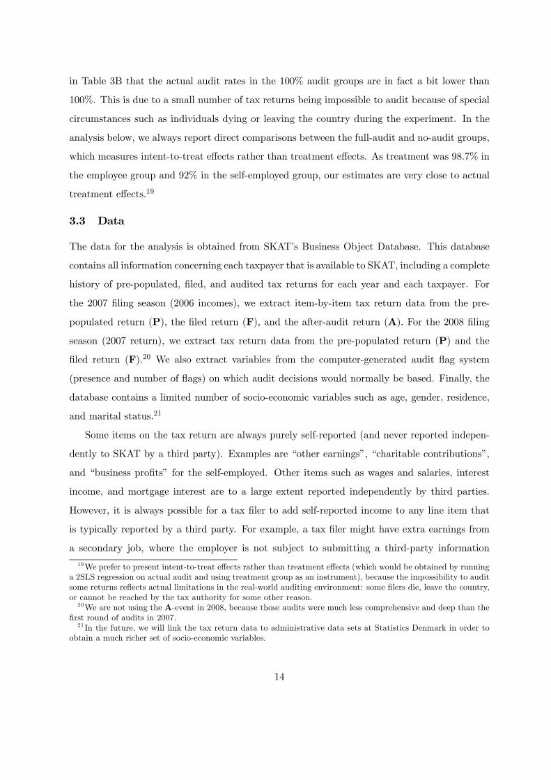
in Table 3B that the actual audit rates in the 100% audit groups are in fact a bit lower than

100%. This is due to a small number of tax returns being impossible to audit because of special

circumstances such as individuals dying or leaving the country during the experiment. In the

analysis below, we always report direct comparisons between the full-audit and no-audit groups,

which measures intent-to-treat effects rather than treatment effects. As treatment was 98.7% in

the employee group and 92% in the self-employed group, our estimates are very close to actual

treatment effects.19

3.3 Data

The data for the analysis is obtained from SKAT’s Business Object Database. This database

contains all information concerning each taxpayer that is available to SKAT, including a complete

history of pre-populated, filed, and audited tax returns for each year and each taxpayer. For

the 2007 filing season (2006 incomes), we extract item-by-item tax return data from the pre-

populated return (P), the filed return (F), and the after-audit return (A). For the 2008 filing

season (2007 return), we extract tax return data from the pre-populated return (P) and the

filed return (F).20 We also extract variables from the computer-generated audit flag system

(presence and number of flags) on which audit decisions would normally be based. Finally, the

database contains a limited number of socio-economic variables such as age, gender, residence,

and marital status.21

Some items on the tax return are always purely self-reported (and never reported indepen-

dently to SKAT by a third party). Examples are “other earnings”, “charitable contributions”,

and “business profits” for the self-employed. Other items such as wages and salaries, interest

income, and mortgage interest are to a large extent reported independently by third parties.

However, it is always possible for a tax filer to add self-reported income to any line item that

is typically reported by a third party. For example, a tax filer might have extra earnings from

a secondary job, where the employer is not subject to submitting a third-party information

19We prefer to present intent-to-treat effects rather than treatment effects (which would be obtained by runninga 2SLS regression on actual audit and using treatment group as an instrument), because the impossibility to auditsome returns reflects actual limitations in the real-world auditing environment: some filers die, leave the country,or cannot be reached by the tax authority for some other reason.20We are not using the A-event in 2008, because those audits were much less comprehensive and deep than the

first round of audits in 2007.21 In the future, we will link the tax return data to administrative data sets at Statistics Denmark in order to

obtain a much richer set of socio-economic variables.

14

report. For tax return items that can be both third-party reported and purely self-reported, we

are currently not able to separate the two components exactly (although we are in the process

of getting this data). At the moment, we therefore define self-reported items as income items

(lines on the tax return) that are always purely self-reported, which is a subset of all self-reported

income items.

4 Empirical Results

4.1 Randomization Test and Baseline Tax Compliance

This section analyzes the tax returns filed and audited in 2007 for incomes earned in 2006

(baseline). The first step is to run a randomization test to ensure that the treatment and

control groups are ex ante identical. Table 4A displays average incomes and percent of tax

filers reporting non-zero incomes for different components on the filed returns (F event) in

the 100% audit group (Column 1) and the 0% audit group (Column 2). The statistics are

estimated using population weights to reflect averages in the full population of tax filers in

Denmark.22 Because filing takes place before the audits and because the baseline audits are

not preannounced, randomization should imply that there are no significant differences across

the two groups. We compute the differences in column (3) and report the standard error of the

difference in column (4). Among the 14 statistics we report, only one is statistically significant

at the 5% level suggesting that indeed the randomization was successful.23

Personal income (defined as the sum of employee earnings, pensions, and transfers) is by

far the largest income component and such income is reported by over 95% of tax filers. As

mentioned above, capital income is negative on average due to mortgage interest payments and

is also very common (94% of tax filers report non-zero capital income). Capital income is about

-5% of personal income on average. Deductions also represent about 5% of personal income on

average, but only 60% of tax filers report deductions. Note that the fraction with deductions

is 60.1% and 61.6% in the audit and no-audit groups, respectively, and is the only statistically

significant difference. Stock income is about 3% of personal income and is reported by about

22% of tax filers. Self-employment income is about 5% of personal income and is reported by

22As noted above, SKAT over-sampled complex returns and returns with self-employment income in order toobtain more precise estimates with a smaller sample.23Because we are looking are many statistics, it is not too surprising that at least one difference will be significant

at the 5% level.

15

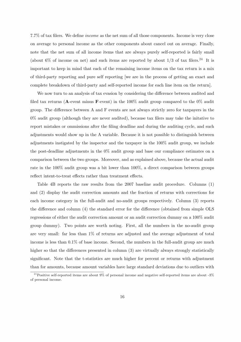
7.7% of tax filers. We define income as the net sum of all those components. Income is very close

on average to personal income as the other components about cancel out on average. Finally,

note that the net sum of all income items that are always purely self-reported is fairly small

(about 6% of income on net) and such items are reported by about 1/3 of tax filers.24 It is

important to keep in mind that each of the remaining income items on the tax return is a mix

of third-party reporting and pure self reporting [we are in the process of getting an exact and

complete breakdown of third-party and self-reported income for each line item on the return].

We now turn to an analysis of tax evasion by considering the difference between audited and

filed tax returns (A-event minus F-event) in the 100% audit group compared to the 0% audit

group. The difference between A and F events are not always strictly zero for taxpayers in the

0% audit group (although they are never audited), because tax filers may take the initative to

report mistakes or ommissions after the filing deadline and during the auditing cycle, and such

adjustments would show up in the A variable. Because it is not possible to distinguish between

adjustments instigated by the inspector and the taxpayer in the 100% audit group, we include

the post-deadline adjustments in the 0% audit group and base our compliance estimates on a

comparison between the two groups. Moreover, and as explained above, because the actual audit

rate in the 100% audit group was a bit lower than 100%, a direct comparison between groups

reflect intent-to-treat effects rather than treatment effects.

Table 4B reports the raw results from the 2007 baseline audit procedure. Columns (1)

and (2) display the audit correction amounts and the fraction of returns with corrections for

each income category in the full-audit and no-audit groups respectively. Column (3) reports

the difference and column (4) the standard error for the difference (obtained from simple OLS

regressions of either the audit correction amount or an audit correction dummy on a 100% audit

group dummy). Two points are worth noting. First, all the numbers in the no-audit group

are very small: far less than 1% of returns are adjusted and the average adjustment of total

income is less than 0.1% of base income. Second, the numbers in the full-audit group are much

higher so that the differences presented in column (3) are virtually always strongly statistically

significant. Note that the t-statistics are much higher for percent or returns with adjustment

than for amounts, because amount variables have large standard deviations due to outliers with

24Positive self-reported items are about 9% of personal income and negative self-reported items are about -3%of personal income.

16

very large incomes and possibly large audit adjustments as well. As we will see later, this implies

that it is much easier to detect effects on probabilities of changing reported amounts than effects

on the reported amounts themselves.

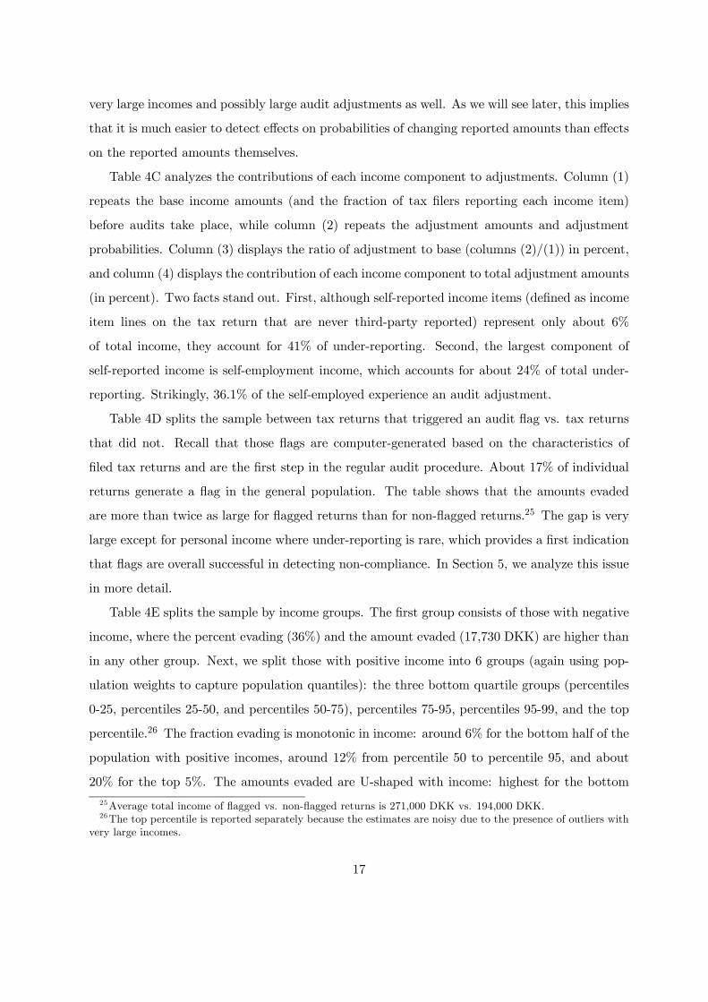
Table 4C analyzes the contributions of each income component to adjustments. Column (1)

repeats the base income amounts (and the fraction of tax filers reporting each income item)

before audits take place, while column (2) repeats the adjustment amounts and adjustment

probabilities. Column (3) displays the ratio of adjustment to base (columns (2)/(1)) in percent,

and column (4) displays the contribution of each income component to total adjustment amounts

(in percent). Two facts stand out. First, although self-reported income items (defined as income

item lines on the tax return that are never third-party reported) represent only about 6%

of total income, they account for 41% of under-reporting. Second, the largest component of

self-reported income is self-employment income, which accounts for about 24% of total under-

reporting. Strikingly, 36.1% of the self-employed experience an audit adjustment.

Table 4D splits the sample between tax returns that triggered an audit flag vs. tax returns

that did not. Recall that those flags are computer-generated based on the characteristics of

filed tax returns and are the first step in the regular audit procedure. About 17% of individual

returns generate a flag in the general population. The table shows that the amounts evaded

are more than twice as large for flagged returns than for non-flagged returns.25 The gap is very

large except for personal income where under-reporting is rare, which provides a first indication

that flags are overall successful in detecting non-compliance. In Section 5, we analyze this issue

in more detail.

Table 4E splits the sample by income groups. The first group consists of those with negative

income, where the percent evading (36%) and the amount evaded (17,730 DKK) are higher than

in any other group. Next, we split those with positive income into 6 groups (again using pop-

ulation weights to capture population quantiles): the three bottom quartile groups (percentiles

0-25, percentiles 25-50, and percentiles 50-75), percentiles 75-95, percentiles 95-99, and the top

percentile.26 The fraction evading is monotonic in income: around 6% for the bottom half of the

population with positive incomes, around 12% from percentile 50 to percentile 95, and about

20% for the top 5%. The amounts evaded are U-shaped with income: highest for the bottom

25Average total income of flagged vs. non-flagged returns is 271,000 DKK vs. 194,000 DKK.26The top percentile is reported separately because the estimates are noisy due to the presence of outliers with

very large incomes.

17

25%, lowest from percentile 25 to percentile 95 and higher in the top 5%. The high evasion

amounts for the bottom quartile are explained by the presence of (relatively) few tax filers with

significant positive and negative incomes which roughly cancel out and who are prone to under-

reporting. As a fraction of income, the rate of evasion is indeed highest in the bottom quartile

(around 15%) and less than 1% in all groups including the top 5%.

Finally, Table 4F brings together the results of Tables 4C, 4D, and 4E by running a sim-

ple OLS regression of an audit adjustment dummy on a number of dummy covariates: income

group (the bottom quartile group is the excluded group), audit flag, self-employment, the pres-

ence of self-reported income, capital income, stock income, and deductions, and finally being

female. This regression is run for the full-audit group and using population weights. The re-

sults confirm our previous findings. Negative income increases the likelihood of misreporting by

16.5%, while other income groups have relatively small effects (once we control for those other

dummy variables). Flags increase the likelihood of underreporting by 18%, being self-employed

increase it by 16%, and having purely self-reporting income increase it by 11%. The presence

of stock income and deductions increases modestly the probability of evading. Interestingly,

being female significantly reduces the probability of evasion by 1.9%.27 These results suggest

that informational setup, type and sign of income have very important effects on evasion. The

only potential sociological or psychological element is the relatively modest effect of gender on

evasion, but it is conceivable that this reflects other dimensions of opportunities to evade (such

as those operating thorugh occupational choice) that we are not yet able to capture. In future

work, we plan to expand our dataset in order to test the sociological or psychological effects

more thoroughly, for example by including variables on occupation, industry, size of business,

ethnic origin, education, etc.

4.2 The Effects of Threat-of-Audit Letters

In order to study the effects of the threat-of-audit letters, we consider the sample of employees

(as the letter randomization did not include the self-employed) who filed tax returns in both

2006 and 2007, and who have an address on record so that they could be reached by mail.

In order to obtain sufficient statistical power, we do two things: (i) we do not use population

weights and (ii) we focus on the probability of making an adjustment from the pre-population

27We also include age controls in the regression but those are not significant.

18

return (P-event) to the final return (F-event) in 2008 with regard to 2007 income. Recall that

the letters were sent to taxpayers shortly after the P-event and about one month prior to the

F-event.

Table 5A presents the effect of letters (100% and 50% letters together) on the probability

of self-reported adjustments in different income components. Columns (1) and (2) display the

probability of such adjustments in the control group (who did not receive the letter) and the

treatment group (who did receive a letter), while column (3) reports the difference between the

two groups (the standard error is reported below the estimate in parenthesis). Columns (4) and

(5) report the effects on upward and downward adjustments separately. As an adjustment is

either upward or downward, column (3) is the sum of columns (4) and (5). Gross income in the

table is defined as the sum of all positive components in total income. Three important findings

emerge.

First, there is a clear significant effect of threat-of-audit letters on the probability of making

an adjustment for all the income components reported in the table. For total income, the prob-

ability increases by 2.17 percentage point from a base of 28%. Among the components of total

income, adjustments are most likely to occur in the self-reported category (base of 25%) and

the adjustment probability is 2.0 percentage points higher among letter recipients. Interestingly,

letters also have an impact on adjustment probabilities for components that are rarely adjusted

such as personal income, capital income, or stock income. Indeed, the proportionate increase

in adjustments is larger for those components than for self-reported income. Second, the ad-

justments reflect primarily upward adjustments as we would expect from the AS model: letters

increase the perceived probability of detection and therefore deter taxpayers from underreport-

ing. Third and perhaps most interesting, we find that the letters also increase the probability of

downward adjustment (which leads to a lower tax liability) for all income components reported

in Table 5A, although none of the differences are statistically significant at the conventional 5%

level (4 of the 6 estimates have a t-statistic above 1.5). In contrast to these results, the AS

model would predict that letters decrease the probability of cheating by making a downward

adjustment to pre-populated income, an important point we come back to later on.

Table 5B splits the sample by 0% and 100% baseline audit. Two additional findings are

worth noting. First, columns (1) and (2) show that letter effects are actually larger in the 0%

audit group than in the 100% audit group. This is clearest for income components, which are

19

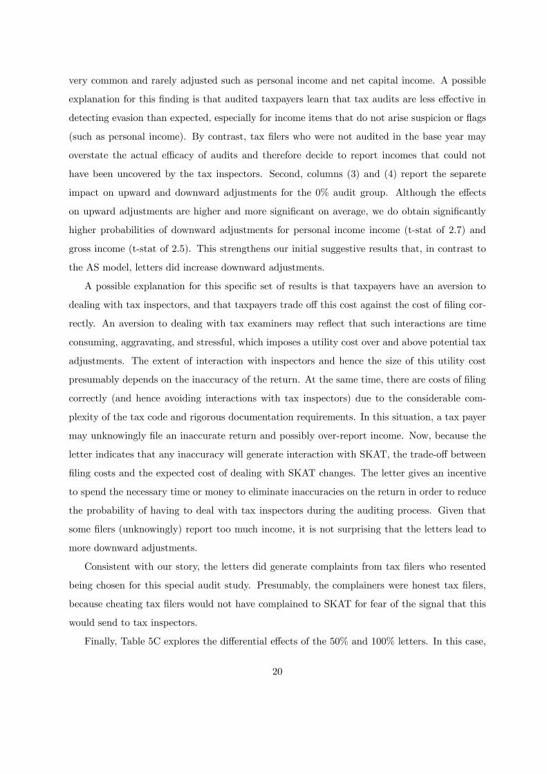
very common and rarely adjusted such as personal income and net capital income. A possible

explanation for this finding is that audited taxpayers learn that tax audits are less effective in

detecting evasion than expected, especially for income items that do not arise suspicion or flags

(such as personal income). By contrast, tax filers who were not audited in the base year may

overstate the actual efficacy of audits and therefore decide to report incomes that could not

have been uncovered by the tax inspectors. Second, columns (3) and (4) report the separete

impact on upward and downward adjustments for the 0% audit group. Although the effects

on upward adjustments are higher and more significant on average, we do obtain significantly

higher probabilities of downward adjustments for personal income income (t-stat of 2.7) and

gross income (t-stat of 2.5). This strengthens our initial suggestive results that, in contrast to

the AS model, letters did increase downward adjustments.

A possible explanation for this specific set of results is that taxpayers have an aversion to

dealing with tax inspectors, and that taxpayers trade off this cost against the cost of filing cor-

rectly. An aversion to dealing with tax examiners may reflect that such interactions are time

consuming, aggravating, and stressful, which imposes a utility cost over and above potential tax

adjustments. The extent of interaction with inspectors and hence the size of this utility cost

presumably depends on the inaccuracy of the return. At the same time, there are costs of filing

correctly (and hence avoiding interactions with tax inspectors) due to the considerable com-

plexity of the tax code and rigorous documentation requirements. In this situation, a tax payer

may unknowingly file an inaccurate return and possibly over-report income. Now, because the

letter indicates that any inaccuracy will generate interaction with SKAT, the trade-off between

filing costs and the expected cost of dealing with SKAT changes. The letter gives an incentive

to spend the necessary time or money to eliminate inaccuracies on the return in order to reduce

the probability of having to deal with tax inspectors during the auditing process. Given that

some filers (unknowingly) report too much income, it is not surprising that the letters lead to

more downward adjustments.

Consistent with our story, the letters did generate complaints from tax filers who resented

being chosen for this special audit study. Presumably, the complainers were honest tax filers,

because cheating tax filers would not have complained to SKAT for fear of the signal that this

would send to tax inspectors.

Finally, Table 5C explores the differential effects of the 50% and 100% letters. In this case,

20

we run an OLS regression on a letter dummy as well as a 100% letter dummy. The 100%

letter dummy measures the additional effect of receiving the 100% letter relative to receiving

the 50% letter. The table shows that there is no clear evidence that the 100% letters generate

more adjustments than the 50% letters. None of the coefficients are significant and the sign is

actually negative in 2 of the 6 regressions we consider. Such results can be explained in the

context of the AS model if an audit probability of 50% is large enough to deter all (detectable)

evasion and push individuals to a corner solution with truthful reporting.

4.3 The Effects of Prior Audits

In order to study the effects of prior audits on subsequent reporting, we consider the sample of

employees and self-employed who file tax returns in both 2006 and 2007. In order to obtain pre-

cise estimates, we do not use population weights and continue to consider effects on probabilities

rather than amounts.

Table 6A focuses on the probability of increasing reported (nominal) income from 2006 to

2007. Columns (1) and (2) show the fraction of filers reporting higher incomes in 2008 than

in 2007 in the 0% audit and 100% audit groups, respectively. Column (3) shows the difference

(column (2) minus column (1)) with standard errors below in parenthesis. We find that prior

audits significantly increase the probability of reporting higher incomes the following year for all

the income components we consider. Consistently, the probability of reporting higher deductions

decreases (although the coefficient is not significant at the 5% level). The effects are strongest

for self-reported income and particularly for self-employment income. This shows that prior

audits are successful in inducing tax filers to increase their reported incomes the following year

although the magnitude of the effects are not very large. The result suggests that being audited

in base year increases the perceived probability of being audited the following year.

Table 6B breaks the sample into subgroups based on being flagged or not in 2006 and on

receiving a letter or not in 2007. In the letter case, the sample is limited to employees. No clear

pattern emerges as different components seem to respond differentially in various subgroups.

21

5 Cost-Benefit Analysis

This section presents a preliminary cost-benefit analysis of tax audits. Throughout the analysis,

we assume that the objective of the tax agency is to maximize tax revenue, i.e.

maxp

(1− p) tz + p (ty + t (y − z) θ)− c · p, (3)

where y should be interpreted as detectable (rather than true) income, c is the audit cost per

return, and the rest of the notation is the same as in section 2.1. In this maximization problem,

the tax agency chooses an audit strategy under exogenously given tax and punishment policies

chosen by policy makers.

Because fines are in practice relatively rare, it makes sense to ignore the effect of auditing

on fine revenue. We consider therefore the revenue effect of increasing the audit rate from p0 to

p1 at θ ' 0:

(p1 − p0) t (y − z0) + (1− p1) t (z1 − z0)− (p1 − p0) · c, (4)

where z0 (z1) is reported income at audit probability p0 (p1). The first term in this expression

is the mechanical recenue effect from the evasion uncovered in tax audits, the second term is the

behavioral revenue effect from evasion deterrence, and the third term is the mechanical revenue

effect from the cost of auditing. In principle, we have an estimate of the first mechanical

revenue effect from the baseline audit regressions and the behavioral revenue effect from the

threat-of-audit letter regressions. However, because we estimated only the effect of letters on

the probability of an income increase rather than the income increase per se, we are currently

not able to quantify the revenue effect of deterrence. However, we will be able to make a number

of interesting points by looking simply at mechanical revenue effects.

Before proceeding, recall that the current audit strategy at SKAT uses automated flags based

on tax return characteristics. All flagged tax returns are in principle looked at by a tax examiner

who then decides whether or not to instigate a full-blown audit based on the severity of flags and

local knowledge. Hence, the current system can be viewed as one where p0 ' 1 for all flagged (f)

tax payers and p0 = 0 for all unflagged (u) taxpayers. Audit increases would therefore include

some unflagged taxpayers, whereas audit reductions would exclude some flagged taxpayers.

Assuming that the deterrence effect (which we do not estimate) is non-negative, we can use

the mechanical revenue effects of auditing to state sufficient (necessary) conditions for increased

22

(reduced) auditing to be optimal. In particular, from eq. (4), a sufficient condition for increased

auditing to be desirable is that for unflagged taxpayers the mechanical revenue effect is positive,

i.e.

tu (yu − zu0 )− cu > 0. (5)

To evaluate this condition, we simply compare the tax revenue uncovered in the baseline audits

to the cost per audited return (which we know from SKAT). Moreover, we may consider a

necessary condition for reduced auditing to be desirable:

tf³yf − zf0

´− cf ≤ 0. (6)

Only if the existing audits are reducing revenue in mechanical terms, is it potentially optimal to

reduce auditing. On the other hand, if the above condition is not satisfied, it is not optimal to

reduce audits in the group of flagged returns, and we therefore want to audit all flagged returns

(because initially p ' 1 in this group). We may also evaluate conditions (5) and (6) for subsets

of unflagged and flagged taxpayers so as to understand whether targeted audit increases or audit

reductions might be optimal.

Our results are shown in Table 7, which presents audit costs and tax revenue for an average

return (yellow), a flagged return (light blue), and an unflagged return (dark blue), and for each

of those categories splits the sample into ‘light’ employees (low-complexity returns), ‘heavy’

employees, self-employed, all employees, and all individuals. It should be noted that the results

reflect the experimental audits, which are more comprehensive and therefore more costly than

regular audits (but which presumably also uncover more income than regular audits).

A number of findings emerge from the table. The first thing to note is that a completely

untargeted audit (average return, all individuals) is close to break even in terms of mechanical

revenue, and therefore is probably revenue increasing when accounting for the deterrence effect.

However, this average effect hides significant heterogeneity across different types of taxpayers,

and the audits are actually generating large revenue losses for the self-employed despite the large

evasion in this group. This is explained by the very costly nature of auditing the self-employed:

tax inspectors spend more than 40 hours on a self-employed filer compared to only 2.2 hours

on an employed filer. The additional cost of auditing self-employed filers is large enough to

dominate the additional tax revenue uncovered among those filers. However, these results lump

23

flagged and unflagged returns together, and as explained above, an evaluation of changes in

current audit strategy has to consider flagged and unflagged returns separately.

To evaluate the scope for audit expansions, we should focus only on the unflagged taxpayers

and consider the sufficient condition (5): if audits of unflagged taxpayers create mechanical

revenue gains, it is surely revenue increasing to instigate those audits. What we see from the

table is that this sufficient condition is not satisfied for the average unflagged taxpayer, but

it is in fact satisfied for unflagged light employees. The cheap nature of those audits and the

non-neglibible income uncovered make those audits profitable.

To evaluate the desirability of audit reductions, we zoom in on the flagged taxpayers and

consider the necessary (6): if this condition is not satisfied, i.e. if audits of flagged taxpayers

create mechanical revenue gains, it is not optimal to reduce audits in this group. Considering the

average flagged return, we see that the audits are indeed generating mechanical revenue gains,

and therefore random reductions in audits of flagged returns (reducing p below 1 for all flagged

returns) are not optimal. This implies that we want to audit all flagged returns unless we can

identify targeted audit reductions for flagged taxpayers that increase revenue. This effectively

amounts to changing the flag-targeting system. What we see from the table is that such targeted

audit reductions may be optimal for self-employed flagged taxpayers, because these audits are

generating large mechanical losses at the margin. This result reflects the combined effect of

these audits being very costly and the fact the flag system does not work very well for the

self-employed. Indeed, the uncovered revenue for flagged self-employed is only slightly higher

than for unflagged self-employed.

To conclude, our results suggest that untargeted audits are pretty close to break even, while

targeted audits are revenue increasing overall. The regular audit targeting procedure based on

automated flags is overall successful in generating revenue, although there seems to be room

for improvement. In particular, there currently seems to be potential over-auditing of the self-

employed relative to (light) employees. This result is driven by the combination of relatively

poor flag-screening for the self-employed, and the fact that it is much more costly to audit the

self-employed than employees.

These results shed some light on the optimal targeting of audits across different taxpayers for

a given type of tax audit (comprehensive audits). Another interesting question is the optimal

targeting across income items for a given type of taxpayer. Audits that target only certain

24

line items on the return are likely to be cheaper, and if the audits target the right items, they

may uncover almost as much revenue as comprehensive audits. In the paper, we have presented

evidence on the type of line items to target, namely line items that have no double reporting by

third parties and are always purely self-reported. However, because we currently do not have a

measure of the cost of audits that target specific line items, we cannot conduct a cost-benefit

analysis for this type of audits.

6 Conclusions and Conceptual Implications

An extensive literature has studied tax evasion and tax enforcement from both the theoretical

and empirical perspective. Following the seminal study by Allingham and Sandmo (1972),

the theoretical literature focuses on a situation where taxpayers decide how much income to

self-report facing a probability of audit and a penalty associates with cheating. In effect, this

type of model considers tax evasion as another risky asset in a household’s portfolio. Micro-

simulations as well as laboratory experiments show that, at realistic levels of audit probabilities

and penalties, an AS-type setting predicts much less compliance than we observe in practice,

at least in developed countries. This suggests that the AS-model misses important aspects

of the real-world reporting environment, and a number of different generalizations have been

proposed and analyzed in the literature. In particular, several authors have argued that observed

compliance levels can only be explained by accounting for psychological aspects of the reporting

decision such as guilt, shame, and a moral obligation to pay taxes.

While we do not deny the importance of psychological aspects in the decision to evade

on taxes, the evidence presented in this paper points to a more classic information story. In

particular, we show that the key distinction in the taxpayer’s reporting decision is whether

the income item in question is subject to information reporting from third parties or if the

information is collected solely by self-reporting (combined with audit threats and penalties).

Unlike previous empirical studies, our data enable us to distinguish precisely between income

items subject to each type of reporting. Only the part of income subject to pure self-reporting

is adequately described by an AS-type setting, and for such income items we do indeed find that

evasion is quite substantial. On the other hand, for the part of income that is subject to third-

party reporting, the government has perfect information unless the taxpayer and the third party

25

collude and jointly underreport income. Our study suggests that, absent such collusion, third-

party reporting is an extremely effective enforcement device. Given the very costly nature of tax

audits and their limited effectiveness is detecting hidden income, we conclude that enforcement

resources are better spent protecting third-party tax bases and extending third-party reporting

rather than traditional audits of self-reported items.

Our findings raise the theoretical question of why third-party reporting works so effectively?

In other words, why don’t taxpayers and third-parties collude to jointly underreporting income?

In a forthcoming companion paper (Kleven, Kreiner, and Saez, 2009), we set out a new theory of

tax evasion providing a mechanism design story that can explain this phenomenon. The model

is three-tiered agency model where the top tier is the government trying to collect taxes from

individual income earners (the bottom tier) who are employed and paid by firms (the middle

tier). Firms are acting as third parties required to double-report income on behalf of their

employees. If the firm is large (and/or if the production process is complex), using accounting

books is very valuable for productivity. The presence of accounting books create common and

verifiable information within the firm. The presence of within-firm common information makes a

collusion equilibrium very fragile, because a single disgruntled employee can destroy the collusion

for everybody in the firm by acting as a whistle-blower. The larger the firm, the more likely

such whistle-blowing will happen. Hence, in an economy with large and complex firms using

accounting books, collusion is not an equilibrium and third-party reporting is effective. This

theory points to the rise of large and complex firms over the economic growth process as the

key factor in making third-party reporting work and therefore in explaining the increasing fiscal

capacity of governments over the course of economic development.

26

References

Allingham, M. G. and A. Sandmo (1972). “Income Tax Evasion: A Theoretical Analysis.”

Journal of Public Economics 1, 323-338.

Alm, J., B. R. Jackson, and M. McKee (1992a). “Deterrence and Beyond: Toward

a Kinder, Gentler IRS,” in J. Slemrod (ed.), Why People Pay Taxes: Tax Compliance and

Enforcement, University of Michigan Press: Ann Arbor, MI.

Alm, J., B. R. Jackson, and M. McKee (1992b). “Estimating the Determinants of Taxpayer

Compliance with Experimental Data.” National Tax Journal 45, 107-114.

Alm, J., B. R. Jackson, and M. McKee (2008). “Getting the Word Out: Enforcement

Information Dissemination and Compliance Behavior.” Journal of Public Economics (in press).

Alm, J., G. H. McClelland, and W. D. Schulze (1992). “Why Do People Pay Taxes?”

Journal of Public Economics 48, 21-38.

Andreoni, J., B. Erard, and J. Feinstein (1998). “Tax Compliance.” Journal of Economic

Literature 36, 818-860.

Beck, P. J., J. S. Davis, and W. Jung (1991). “Experimental Evidence on Taxpayer

Reporting under Uncertainty.” Accounting Review 66, 535-558.

Becker, G. S. (1968). “Crime and Punishment–An Economic Approach.” Journal of Political

Economy 76, 169-217.

Becker, W., H. J. Buchner, and S. Sleeking (1987). “The Impact of Public Transfer

Expenditures on Tax Evasion; an Experimental Approach.” Journal of Public Economics 34,

243-252.

Beron, K. J., H. V. Tauchen, and A. D. Witte (1992). “The Effect of Audits and

Socioeconomic Variables on Compliance,” in J. Slemrod (ed.), Why People Pay Taxes: Tax

Compliance and Enforcement, University of Michigan Press: Ann Arbor, MI.

Bloomquist, Kim M. (2003). “Tax Evasion, Income Inequality and Opportunity Costs of

Compliance”, 96th National Tax Association Conference.

Christian, Charles W. “Voluntary Compliance With The Individual Income Tax: Results

From the 1988 TCMP Study,” The IRS Research Bulletin, IRS Publication 1500 (Rev.9-94),

(1993/1994): 35-42.

Dubin, J. A. and L. L. Wilde (1988). “An Empirical Analysis of Federal Income Tax

Auditing and Compliance.” National Tax Journal 41, 61-74.

27

Dubin, J., M. Graetz, L. Wilde (1990). “The effect of audit rates on the federal individual

income tax, 1977-1986.” National Tax Journal 43, 395-409.

Friedland, N., S. Maital, and A. Rutenberg (1978). “A Simulation Study of Income Tax

Evasion.” Journal of Public Economics 10, 107-116.

Internal Revenue Service. Federal Tax Compliance Research: Individual Income Tax Gap

Estimates for 1985, 1988, and 1992, IRS Publication 1415 (Rev. 4-96), Washington, D.C., 1996.

Klepper, Steven and Daniel Nagin (1989). “The Anatomy of Tax Evasion,” Journal of

Law, Economics, and Organization 5(1), 1-24.

Kleven, Henrik, Kreiner, Claus, and Emmanuel Saez (2009). “Why Can Modern Gov-

ernments Tax So Much? An Agency Model of Firms as Fiscal Intermediaries” Working paper

(draft in Progress).

Long, Susan, and Judyth Swingen. “Third Party Information Reporting and Compliance.”

In Research Conference Report, How Do We Affect Taxpayer Behavior?, Internal Revenue Ser-

vice Document 7302 (3-91), Washington, D.C., 1990.

Pommerehne, W. W. and B. Frey (1992). “The Effects of Tax Administration on Tax

Morale.” Unpublished manuscript, University of Saarbrucken.

Slemrod, J., M. Blumenthal, and C. Christian (2001). “Taxpayer response to an increased

probability of audit: evidence from a controlled experiment in Minnesota.” Journal of Public

Economics 79, 455-483.

Slemrod, J. and S. Yitzhaki (2002). “Tax avoidance, evasion and administration,” in A.J.

Auerbach and M. Feldstein (eds.), Handbook of Public Economics, Vol. 3, Elsevier: Amsterdam.

Yitzhaki, S. (1974). “A Note on Income Tax Evasion: A Theoretical Analysis.” Journal of

Public Economics 3, 201-202.

28

Audit of 2006 tax return

100% Audit Group 0% Audit Group

Not to be touched

Oct 1, 2007

May 1, 2007

Figure 1. Experimental Design for Employees

100% Letter

May 1, 2008

50% LetterNo Letter

Audit of 50% of all 2007 tax returns

No further action

Data collection: tax and audit data from SKAT’s Business Object Database

Jan 1, 2009

Audit of all 2007 tax returns

Aug 1, 2008

Data collection: link SKAT data with administrative datasets at Statistics Denmark

100% Letter50% Letter

No further action

No Letter

Threat-of-audit letter with regard to 2007 return (50%)

1/3

Audit of 50% of all 2007 tax returns

No further action

Audit of all 2007 tax returns

April 1, 2008

Letter informs tax payer of audit result No action

Threat-of-audit letter with regard to 2007 return (100%)

1/3 1/3 1/3 1/3 1/3

No further action

Threat-of-audit letter with regard to 2007 return (50%)

Threat-of-audit letter with regard to 2007 return (100%)

Table 1. Income concepts in the Danish individual income tax in 2006

Income concept Main items included

1. Labor income Salary, wages, honoraria, fees, bonuses, fringe benefits, business earnings

2. Personal income Labor income (1) + transfers, grants, awards, gifts, received alimony— labor market tax, certain pension contributions

3. Capital income Interest income, rental income, business capital income— interest on debt (mortgage, bank loans, credit cards, student loans)

4. Deductions Commuting, union fees, UI contributions, other work expenditures,charity, paid alimony

5. Taxable income Personal income (2) + capital income (3) - deductions (4)

6. Share income Dividends and realized capital gains from shares

Table 2. Tax rates and tax bases in the Danish individual income tax in 2006

Tax type Tax base Bracket (DKK)1 Rate (%)

Labor market tax Labor income All income 8.0

EITC Labor income up to 300.000 2.5

Bottom Tax Personal income + capital income if > 0 38,500- 5.5

Middle Tax Personal income + capital income if > 0 265,500- 6.0

Top Tax Personal income + capital income if > 0 318,700- 15.02

Regional tax Taxable income 38,500- 32.63

Tax on shares Share income 0-44,400; 44,400- 28.0; 43.0

1. All amounts in Danish Kroner (DKK). 6 DKK ' 1 USD.2. This rate may be affected by a tax ceiling on the total marginal tax rate (see below).3. The regional tax includes municipal + county taxes in 2006. The rate shown is the average across allmunicipalities, and includes an optional church tax equal to 0.7%.

Self-employed

100% Audit 14,280 obs. 8890 obs.Group

population weights pop weights0% Audit 14,280 obs. 8874 obs.Group

population weights pop weights

Self-employed

100% Audit 10,740 obs.=14,280 -3,540 reduction 8890 obs.Group Audit rate: 98.7% Audit: 92%

reweight to pop weights pop weights0% Audit 14,280 obs. (no reduction) 8874 obs.Group Audit rate: 0% Audit: 0%

population weights pop weights

Note: audit group was reduced (in a random stratified way). Baseline tax compliance: compare blue and yellow tax returns after audit in base year

Employees

Employees

3A. Base Year: Tax Compliance Study (plan)

3B. Base Year: Tax Compliance Study (actual)

Note: tax returns selected in 2007 and stratified by (a) self-employment (b) return complexity (c) geo location

Self-employed

100% audit letter

50% audit letter No letter No letter

100% Audit 3419 obs. 3408 obs. 3407 obs. 8320 obs.Group

0% Audit 4001 obs. 3996 obs. 5709 obs. 8342 obs.Group

reweight reweight reweight

Self-employed

100% audit letter

50% audit letter No letter No letter

100% Audit 3419 obs. 3408 obs. 3407 obs. 8320 obs.Group

0% Audit 4001 obs. 3996 obs. 5709 obs. 8342 obs.Group

reweight reweight reweight

Reweight 0% audit groups to match 100% audit groups. Some could not be reached by letter or dropped out. Letter effects: compare blue, light blue, and yellow tax returns in post year

Effect of base-year audit on post-year reported income: compare blue and yellow tax returns in post year

3C. Post Year: Letter Effects

Employees

3D. Post Year: Prior-Audit Effects

Employees

100% audit 0% audit

100%-0% (s.e)

Personal Income (amt) 208,866 209,982 -1,116 (1830)% with personal income 95.2 95.1 0.1 (0.2)Capital Income, (net amt) -11,000 -10,928 -81 (505)% with capital income 93.9 93.8 0.2 (0.2)Deductions (amt) -9,109 -9,331 221 (140)% with deductions 60.1 61.6 -1.60 (0.47)Stock Income (amt) 5,572 7,328 -1,756 (3172)% with stock income 22.5 22.2 0.3 (0.4)Self-Employment (amt) 10582 10567 15 (1269)% with self-employment 7.7 7.7 0.10 (0.26)Income = PI+CI+D+SI+SE 205,376 208,257 -2,882 (3873)% with income 98.4 98.2 0.16 (0.12)Self-Reported Income (amt) 12115 11684 431 (1756)% with self-reported inc. 32.9 33.6 -0.68 (0.46)# obs. 19,630 23,148 42,778Amounts in Danish Kroner: 10 DKK = 1 GBP = US $2 [POP. WEIGHTED]Bold for 5% significant.

4A. Randomization Test: Reported Incomes Before Audit

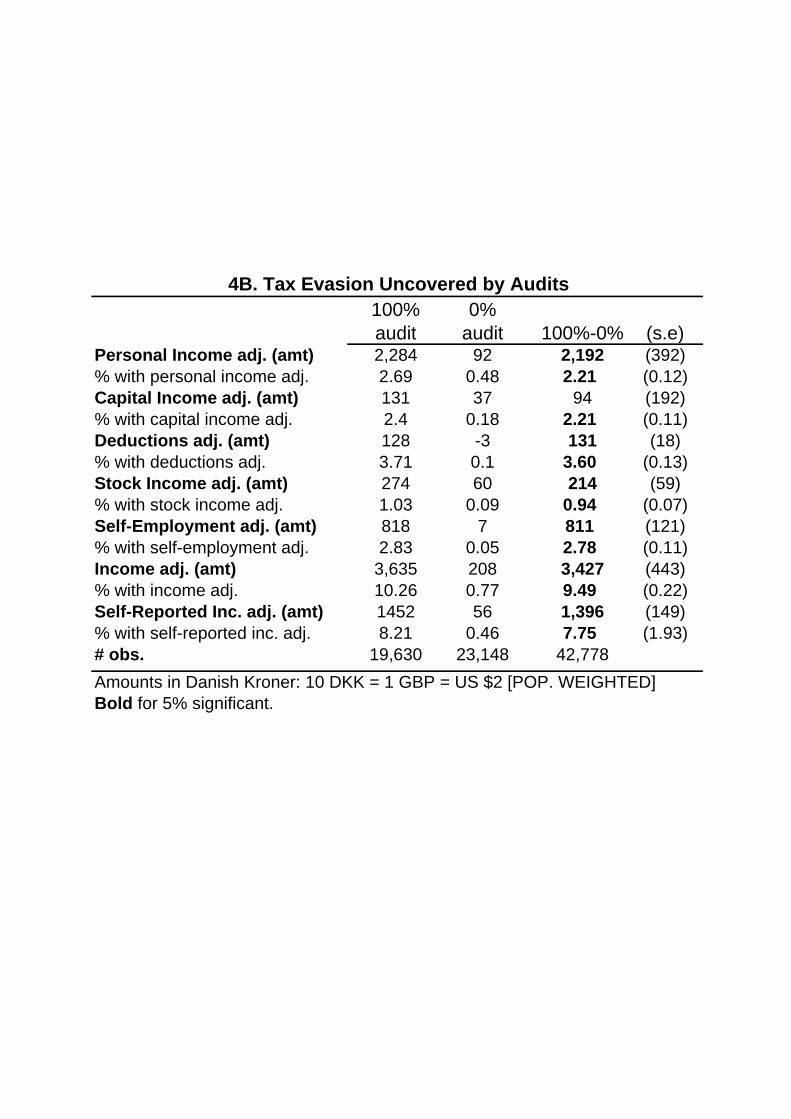
100% audit

0% audit 100%-0% (s.e)

Personal Income adj. (amt) 2,284 92 2,192 (392)% with personal income adj. 2.69 0.48 2.21 (0.12)Capital Income adj. (amt) 131 37 94 (192)% with capital income adj. 2.4 0.18 2.21 (0.11)Deductions adj. (amt) 128 -3 131 (18)% with deductions adj. 3.71 0.1 3.60 (0.13)Stock Income adj. (amt) 274 60 214 (59)% with stock income adj. 1.03 0.09 0.94 (0.07)Self-Employment adj. (amt) 818 7 811 (121)% with self-employment adj. 2.83 0.05 2.78 (0.11)Income adj. (amt) 3,635 208 3,427 (443)% with income adj. 10.26 0.77 9.49 (0.22)Self-Reported Inc. adj. (amt) 1452 56 1,396 (149)% with self-reported inc. adj. 8.21 0.46 7.75 (1.93)# obs. 19,630 23,148 42,778Amounts in Danish Kroner: 10 DKK = 1 GBP = US $2 [POP. WEIGHTED]Bold for 5% significant.

4B. Tax Evasion Uncovered by Audits

BaseAudit adj.

Adj./ Base

Share adj.

Personal Income adj. (amt) 209,424 2,192 1.0% 64%% with personal income adj. 95.2 2.2 2.3%Capital Income adj. (amt) -10,964 94 -0.9% 3%% with capital income adj. 93.9 2.2 2.4%Deductions adj. (amt) -9,220 131 -1.4% 4%% with deductions adj. 60.9 3.6 5.9%Stock Income adj. (amt) 6,450 214 3.3% 6%% with stock income adj. 22.4 0.9 4.2%Self-Employment adj. (amt) 10,575 811 7.7% 24%% with self-employment adj. 7.7 2.8 36.1%Income adj. (amt) 206,817 3,427 1.7% 100%% with income adj. 98.3 9.5 9.7%Self-Reported Inc. adj. (amt) 11,900 1,396 11.7% 41%% with self-reported inc. adj. 33.3 7.8 23.3%Amounts in Danish Kroner: 10 DKK = 1 GBP = US $2 [POP. WEIGHTED]

4C. Tax Evasion Uncovered by Audits: Summary

Evasion Flag (s.e) No Flag (s.e)

Personal Income adj. (amt) 2,592 (543) 2,124 (476)

Capital Income adj. (amt) 25 (905) 107 (87)

Deductions adj. (amt) -550 (67) -59 (16)

Stock Income adj. (amt) 1,065 (285) 69 (23)

Self-Employment adj. (amt) 2367 (447) 544 (104)

Income adj. (amt) 6,539 (1079) 2,895 (491)

Self-Reported Inc. adj. (amt) 4671 (574) 834 (121)

# obs. 11,338 31,440Amounts in Danish Kroner: 10 DKK = 1 GBP = US $2 [POP. WEIGHTED]Bold for 5% significant.

4D. Tax Evasion by Groups: Flag vs. No Flag

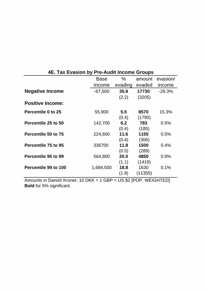
Base Income

% evading

amount evaded

evasion/ income

Negative Income -67,500 35.8 17730 -26.3%(2.2) (3205)

Positive Income:Percentile 0 to 25 55,900 5.5 8570 15.3%

(0.4) (1790)Percentile 25 to 50 142,700 6.2 783 0.5%

(0.4) (185)Percentile 50 to 75 224,600 11.6 1155 0.5%

(0.4) (306)Percentile 75 to 95 336700 11.8 1500 0.4%

(0.5) (289)Percentile 95 to 99 564,800 20.0 4850 0.9%

(1.1) (1419)Percentile 99 to 100 1,684,500 18.8 1630 0.1%

(1.9) (11355)Amounts in Danish Kroner: 10 DKK = 1 GBP = US $2 [POP. WEIGHTED]Bold for 5% significant.

4E. Tax Evasion by Pre-Audit Income Groups

% evading (s.e.)Constant 2.9 (0.9)Negative Income 16.5 (1.8)Percentile 25 to 50 -0.5 (0.6)Percentile 50 to 75 -0.1 (0.7)Percentile 75 to 95 -3.0 (0.7)Percentile 95 to 99 0.8 (1.2)Percentile 99 to 100 -4.8 (2.1)Automatic Evasion Flag 18.1 (0.6)Self-employed 15.7 (0.8)Self-reported income 10.6 (0.5)Capital income 0.5 (0.9)Stock Income 1.1 (0.5)Deductions 2.7 (0.5)Female -1.9 (0.4)

4F. Income Tax Evasion Determinants

Single OLS regression of adj. dummy on dummy covariates [POP WEIGHTED]. Bold for 5% significant.

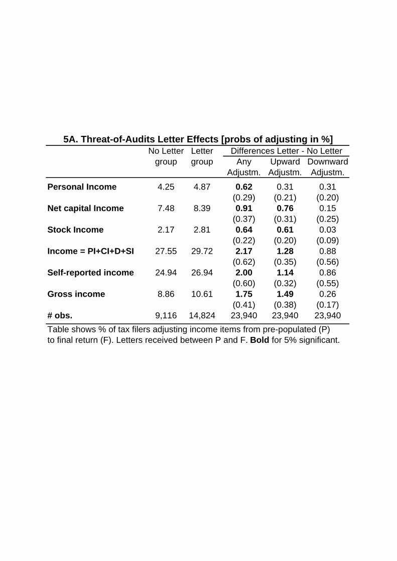
No Letter Lettergroup group

Personal Income 4.25 4.87 0.62 0.31 0.31(0.29) (0.21) (0.20)

Net capital Income 7.48 8.39 0.91 0.76 0.15(0.37) (0.31) (0.25)

Stock Income 2.17 2.81 0.64 0.61 0.03(0.22) (0.20) (0.09)

Income = PI+CI+D+SI 27.55 29.72 2.17 1.28 0.88(0.62) (0.35) (0.56)

Self-reported income 24.94 26.94 2.00 1.14 0.86(0.60) (0.32) (0.55)

Gross income 8.86 10.61 1.75 1.49 0.26(0.41) (0.38) (0.17)

# obs. 9,116 14,824 23,940 23,940 23,940Table shows % of tax filers adjusting income items from pre-populated (P)to final return (F). Letters received between P and F. Bold for 5% significant.

5A. Threat-of-Audits Letter Effects [probs of adjusting in %]Differences Letter - No Letter

Any Adjustm.

Downward Adjustm.

Upward Adjustm.

Personal Income 1.28 -0.04 0.55 0.73(0.38) (0.44) (0.27) (0.27)

Net capital Income 1.44 0.38 1.01 0.43(0.70) (0.58) (0.41) (0.29)

Stock Income 0.60 0.68 0.40 0.20(0.28) (0.34) (0.24) (0.13)

Income = PI+CI+D+SI 2.28 2.06 1.24 1.03(0.82) (0.95) (0.46) (0.75)

Self-reported income 2.08 1.91 1.49 0.58(0.80) (0.92) (0.42) (0.73)

Gross income 2.22 1.29 1.68 0.54(0.54) (0.64) (0.49) (0.22)

# obs. 13,706 10,234 13,706 13,706

Table shows % of tax filers adjusting income items from pre-populated (P)to final return (F). Letters received between P and F. Bold for 5% significant.

5B. Threat-of-Audit Letter Effects: 0% vs 100% Audit GroupDifferences Letter - No Letter

0% audit (any adj.)

0% audit (downward)

100% audit (any adj.)

0% audit (upward)

Personal Income 0.77 -0.31(0.33) (0.33)

Net capital Income 0.64 0.53(0.43) (0.43)

Stock Income 0.50 0.28(0.25) (0.25)

Income = PI+CI+D+SI 2.20 -0.06(0.72) (0.72)

Self-reported income 1.92 0.14(0.70) (0.70)

Gross income 1.34 0.82(0.48) (0.48)

# obs. 23,940 23,940

Table shows % of tax filers adjusting income items from pre-populated (P)to final return (F). Letters received between P and F. Bold for 5% significant.

5C. Threat-of-Audits Letter Effects: 50% vs. 100% LetterDifferences Letter - No Letter (any adjustment)50% letter - no letter 100% letter - 50% letter

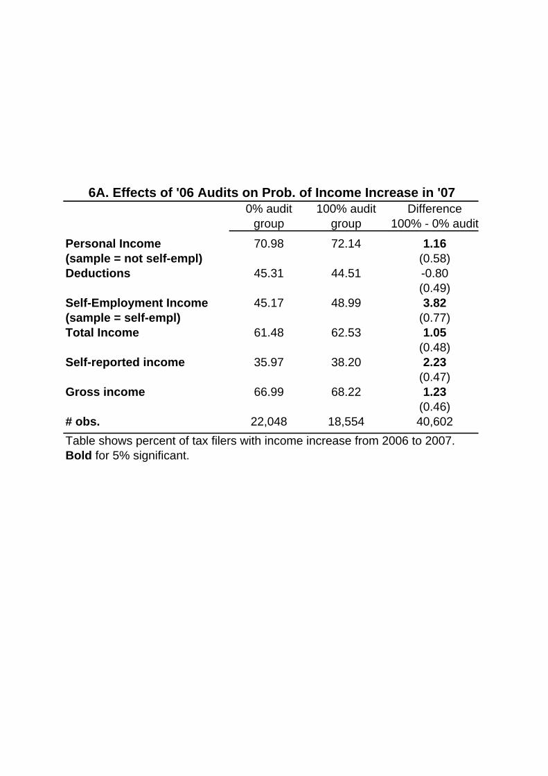
0% audit 100% audit Differencegroup group 100% - 0% audit

Personal Income 70.98 72.14 1.16(sample = not self-empl) (0.58)Deductions 45.31 44.51 -0.80

(0.49)Self-Employment Income 45.17 48.99 3.82(sample = self-empl) (0.77)Total Income 61.48 62.53 1.05

(0.48)Self-reported income 35.97 38.20 2.23

(0.47)Gross income 66.99 68.22 1.23

(0.46)# obs. 22,048 18,554 40,602Table shows percent of tax filers with income increase from 2006 to 2007.Bold for 5% significant.

6A. Effects of '06 Audits on Prob. of Income Increase in '07

Personal Income 0.98 1.19 -0.06 1.76(sample = not self-empl) (1.35) (0.64) (0.94) (0.74)Deductions -1.87 -0.41 -1.99 -0.48

(0.96) (0.57) (1.03) (0.81)Self-Employment Income 3.11 4.22(sample = self-empl) (1.28) (0.97)Total Income 1.00 1.07 0.83 1.33

(0.95) (0.56) (0.99) (0.78)Self-reported income 2.44 2.17 1.68 1.14

(0.96) (0.55) (0.91) (0.73)Gross income 1.09 1.28 0.29 1.64

(0.93) (0.53) (0.94) (0.74)# obs. 10,760 29,842 9,116 14,824Percent of tax filers with adjustments after filing final return F in 2007Bold for significant at 5% level.

No letter in 2007

Letter in 2007

6B. Effects of '06 Audits on Prob. of Income Increase in '07Flag in 2006

No Flag in 2006

pop obs flag audit hours audit cost revenue gain audit cost revenue gain audit cost revenue gainTaxpayer type share share share avg avg avg flag flag no flag no flag

Light employees 0.62 0.14 0.04 2.2 733 1845 733 5403 733 1555Heavy employees 0.30 0.41 0.36 2.4 813 808 813 2231 813 378Self-employed 0.09 0.45 0.60 41.1 13873 5120 13873 5293 13873 5023All employees 0.91 0.55 0.40 2.2 759 1506 782 3479 756 1221All individuals 1.00 1.00 1.00 5.6 1886 1817 3464 3851 1535 1446

Results are population weightedAmounts in Danish Kroner (10 DKK = 1 GBP) Cost per audit hour (salaray and overhead) equals 338 DKK = 33.8 GBP

TABLE 7. COST-BENEFIT ANALYSIS FOR TAX AUDITS