an index of diversity and the relation of certain concepts ...(margaleff 1958, macarthur and...

An Index of Diversity and the Relation of Certain Concepts to DiversityAuthor(s): Robert P. McIntoshSource: Ecology, Vol. 48, No. 3 (May, 1967), pp. 392-404Published by: Ecological Society of AmericaStable URL: http://www.jstor.org/stable/1932674Accessed: 12/12/2010 23:43

Your use of the JSTOR archive indicates your acceptance of JSTOR's Terms and Conditions of Use, available athttp://www.jstor.org/page/info/about/policies/terms.jsp. JSTOR's Terms and Conditions of Use provides, in part, that unlessyou have obtained prior permission, you may not download an entire issue of a journal or multiple copies of articles, and youmay use content in the JSTOR archive only for your personal, non-commercial use.

Please contact the publisher regarding any further use of this work. Publisher contact information may be obtained athttp://www.jstor.org/action/showPublisher?publisherCode=esa.

Each copy of any part of a JSTOR transmission must contain the same copyright notice that appears on the screen or printedpage of such transmission.

JSTOR is a not-for-profit service that helps scholars, researchers, and students discover, use, and build upon a wide range ofcontent in a trusted digital archive. We use information technology and tools to increase productivity and facilitate new formsof scholarship. For more information about JSTOR, please contact [email protected].

Ecological Society of America is collaborating with JSTOR to digitize, preserve and extend access to Ecology.

http://www.jstor.org

http://www.jstor.org/action/showPublisher?publisherCode=esa

http://www.jstor.org/stable/1932674?origin=JSTOR-pdf

http://www.jstor.org/page/info/about/policies/terms.jsp

http://www.jstor.org/action/showPublisher?publisherCode=esa

392 ROBERT P. McINTOSH Ecolov. Vol. 48. No. 3

90%o of the tests performed the results of the first. en- counter were confirmed in subsequent encounters.

APPENDIX II

In the behavioural repertoire of the male, threat be- haviour, chasing, fighting, and aggressive grooming may be regarded as good indicators of aggressive interaction. The question is, which of these acts, or what combination of them, is the most sensitive indicator of aggressiveness

in males? This question was partly answered by plotting each act against the sum of all four acts for each bout. Data from the control series in the experiments on sea- sonal changes in aggressiveness were used. The four resulting scatter diagrams are shown in Figure 5. Threats and chases show a consistent relation to total aggression, while fights and aggressive grooming appear to add only a random factor. Hence the sum of threats and chases was chosen as the most sensitive index of aggressiveness.

AN INDEX OF DIVERSITY AND THE RELATION OF CERTAIN CONCEPTS TO DIVERSITY

ROBERT P. MCINTOSH Department of Biology, University of Notre Dame, Notre Dame, Indiana

(Accepted for publication August 10, 1966)

Abstract. The uses in ecology of the terms richness, diversity, homogeneity, and similarity are considered in the context of recent studies of plant and animal communities. Various uses of diversity are reviewed and an index of diversity derived from the distance measure

of similarity is suggested. This index is < I2n 2 where S equals the number of species and

n equals the number of individuals in each species. This index is compared with other indices of diversity. The principal problem of measuring diversity is the assessment of the homogeneity or similarity of the sample or samples being studied. An advantage of the proposed index is that it derives from a measure of similarity of which it is a special case, and it is a more natural and familiar representation of points in a coordinate system.

INTRODUCTION

The concept of diversity is particularly important because it is commonly considered an attri- bute of a natural or organized community (Hair- ston 1964) or is related to important ecological processes. Diversity has been said to increase in a successional sequence to a maximum at climax, to enhance community stability, and to relate to community productivity, integration, evolution, niche structure, and competition. All of these are controversial and important ecological concepts. Specific models of the distribution of individuals among species have been used to define communities. Clarification of the concept of diversity, its relation to other ecological concepts, and agree- ment as to its use and measurement are, therefore, more than matters for semantic wrangling. A number of quantitative indices of diversity have been proposed (Fisher, Corbett, and Williams 1943, Simpson 1949, MacArthur 1957, Margaleff 1958, Odum, Cantlon, and Kornicker 1960). This paper is concerned with the concept of diversity as it is related to the biotic community and its properties. The concept of diversity in describing the biota of geographical or biotic regions including widely differing habitats and communities is not considered.

Charles Elton (1949) observed that the study of communities has largely been the province of

plant ecologists, while the study of populations has been the domain of the animal ecologist. This view must be modified in the light of much recent discussion by animal ecologists about the organization and properties of the animal community, its relation to the plant community, or their incor- poration into the ecosystem. Particular attention has been given to the distribution of numbers of individuals among the species of a community (Preston 1948, 1962, Margaleff 1958, Hairston 1959, 1964, Odum, Cantlon, and Kornicker 1960, MacArthur 1960, 1964, Lloyd and Ghelardi 1964, King 1964, Menhinick 1964, Tagawa 1964). The property of number, called abundance by some animal ecologists or density by others and by most plant ecologists, I will call density. The distribution of numbers of individuals (or other quantities such as biomass or productivity) among the species of a community has long been regarded as of great importance in the study of the organization of the community. Gause (1936) commented that the most important structural property of a community is a definite quantitative relationship he- tween abundant and rare species, and the signifi- cance attached to this relationship is apparent in recent studies (Hairston 1959, 1964, MacArthur 1957, 1960, MacArthur and MacArthur 1961, Whittaker 1952, 1960, 1964). Hairston (1959) for example states, ". . . numerical abundance and

Late Spring 1967 INDEX OF DIVERSITY 393

spatial distribution of all species must be taken into account before an understanding of community organization can be obtained."

Plant ecologists have commonly used the relation of species to area (species-area curve), which reflects the relative numbers of individuals of several species, as an indication of the distribution of numbers of individuals among the species. Such curves have been used to define the community or to indicate the minimum area required for adequate representation of species of a community (Goodall 1952, Greig-Smith 1964). Only occa- sionally have plant ecologists considered species- individual relationships directly (Black, Dobzhan- sky, and Pavan 1950). Animal ecologists have been concerned largely with species-individual relations, usually within a limited taxonomic group at the level of family or class. One reason suggested for this difference is the relative ease of distinguishing the individual animal as compared to the plant individual (Dahl 1956, Greig-Smith 1964, Whittaker 1964, Williams 1964). Hairston (1959) lists many of the various approaches to community analysis based on species composition and the distribution of numbers of individuals among the species.

A number of terms are commonly used in discussions of community ecology sometimes with different, overlapping, or synonymous meanings. Most widely used are the antonyms: poor- rich, uniform-diverse, homogeneous-heterogeneous, similar-different. All have been applied to the habitat as well as to the community of organisms, but it is only the latter usage which is considered in this paper. Other words, e.g., simple-complex, close-distant, may be used with similar connotations to the more familiar ones.

Rich and poor in common biological parlance indicate simply the number of species present and are so used here. Rich may be used as synonymous with diverse as defined below (Black et al. 1950, Curtis 1959, Whittaker 1960, 1964, Connell and Orias 1964). Diversity has been widely used, particularly in connection with recent studies of animal communities. It usually incorporates, in addition to the number of species (richness), the distribution of individuals among the species (Margaleff 1958, MacArthur and MacArthur 1961, Lloyd and Ghelardi 1964). Lloyd and Ghelardi state this most succinctly in recognizing two components of diversity, species number (richness) and "equitability," the distribution of individuals among the species. Their "equitability" component corresponds inversely with Whittaker's (1964) "dominance concentration." Diversity will be used throughout this paper in the sense of Lloyd and Ghelardi, incorporating

both richness and equitability. Communities with the same richness may differ in diversity depend- ing upon the distribution of the individuals among the species. Maximum diversity results if individuals are distributed equally among species; concentration of numbers or other measure of quantity (dominance in Whittaker's (1964) sense) in one or a few species decreases diversity which is minimal (0) if all individuals are of one species.

Homogeneity has long been stressed as being of fundamental importance in studies of the plant community (Goodall 1952, 1954, Dahl 1956, Greig-Smith 1964). It is usually synonymous with uniformity (Dahl 1956). Plant ecologists have usually used a subjective or intuitive estimate of similar appearance and composition to assess homogeneity, but in a stricter sense a plant species is considered homogeneously distributed if the mean number of individuals is the same in all parts of an area, i.e., if the probability of encoun- tering the species is the same. Some authors have restricted the term to species which are randomly distributed or, if clumped, which have the clumps randomly distributed (Curtis and McIntosh 1950, Margaleff 1958); others (Dahl 1956) apply it to regular as well as random or clumped distributions. Catana (1964) calls non-random distributions homogeneous if the degree of non-random- ness is the same throughout the area studied. In multi-species communities a test of homogeneity in the statistical sense has rarely been applied to other than the most common species (Curtis and McIntosh 1951), and normally homogeneity is determined subjectively. Communities which will meet any or all of the statistical measures of spatial homogeneity are rare or, in any case, rarely demonstrated to be homogeneous by such measures.

Plant ecologists have assessed homogeneity by the relationship of number of species to area (species-area curves) (Poore 1964) or by the distribution of species frequencies in classes according to Raunkiaer's "law of frequency" (Dahl 1956, McVean and Ratcliffe 1962). Species- area curves and frequency distributions are based upon an ill-defined amalgam of richness, diversity, sample size, and species distribution in space which renders them highly suspect as defining homogeneity (McIntosh 1962, Greig-Smith 1964). More recently the relation of variance between samples to the distance between the samples and lack of significant correlations between species have been suggested as indications of homogeneity (Goodall 1954, Williams and Lambert 1959, Dahl 1960).

Homogeneity has been considered in the spatial sense by animal ecologists, and Hutchinson (1953)

394 ROBERT P. McINTOSH Ecology, Vol. 48, No. 3

has categorized the causes of departure from homogeneity, i.e., heterogeneity. Some animal ecologists have considered diversity as a criterion of homogeneity (Hairston 1959, MacArthur 1960). MacArthur's (1957) model of diversity in which the densities of the species are assumed to be randomly distributed among the species has been asserted to fit some animal communities (Kohn 1959, MacArthur 1960). Others have found animal groups which do not fit the model (Hairston 1964, King 1964). MacArthur and Kohn state that increasing the homogeneity of the sample results in a closer fit of the data to MacArthur's model. Hairston (1959) and Tur- ner (1961), however, found that increased heterogeneity resulted in a closer fit to MacArthur's model. King (1964) attempts to reconcile this contradiction. Whittaker (1964) found that plant species in a variety of vegetation types did not fit MacArthur's model. The model therefore is suggested as an indication of homogeneity in a natural community, and departures from it are presumed to be caused by heterogeneity in the community.

Hutchinson (1958) applied the term "homogeneously diverse" to an area where the scale of environmental variation is small relative to the movements of the animal concerned and "heterogeneously diverse" to an area which includes differences in habitat, cf. woodland and pasture. King (1964) notes that MacArthur's model is applicable only in a homogeneously diverse area. However, there is no indication that any test of homogeneity has been applied in the various papers cited above other than the fit to Mac- Arthur's model. Although animal ecologists have studied the distribution of individual species, like the plant ecologists they rarely apply statistical tests of homogeneity in community studies. Hair- ston (1964) assesses homogeneity on the ubiquity of distribution of bird species in a number of subjectively recognized vegetational habitats. This is reminiscent of the methods of many plant ecologists.

There is a widespread view that organisms are distributed in nature in aggregations or communities which are homogeneous within themselves and heterogeneous between two or more such aggregations (Goodall 1954). Some plant ecologists have elevated the recognition of uniform or homogeneous plant community to an art (Dahl 1956, Becking 1957). Some animal ecologists, tacitly at least, agree in recognizing a homogeneous community having statistical properties which change if heterogeneous material is included from another community (Hairston 1959, King 1964). Richness and diversity have commonly

been described as a characteristic property of a putative homogeneous community and indicative of its organization. Lambert and Dale (1965), on the other hand, comment that homogeneity has little use in ecological studies. They prefer to regard vegetation as a heterogeneous system and to reduce the heterogeneity by arbitrary methods to statistically defined levels acceptable for the purpose of a particular study. A technique for doing this has been proposed (Williams and Lambert 1959) which seeks to identify homogeneous groups of samples in which statistically significant correlations between species are absent. In small areas it has given interesting results. However, it is a monothetic method involving a rigid series of successive divisions. Beckner (1959) points out that the possibility of error is great in such methods. He notes also that monothetic methods do not yield natural groups although they may produce useful and clear classi- fications. A further problem of the technique is that the sequence of choices and hence the resultant groups will be markedly affected by the size of the sample used (Kershaw 1961, Austin, personal communication).

It is essential to keep in mind that the term homogeneity is commonly used by ecologists in two senses (Greig-Smith 1964): (1) It is applied, as noted above, to the spatial distribution of species in a single plot of a community or in a stand (the concrete community in the sense of the plant ecologist). (2) It may also apply to a comparison of data derived from several separate communities or stands with no reference to spatial pattern. In the concept of stand or community unit there is commonly an assumption of a considerable degree of homogeneity in the first or spatial sense. Stand sometimes connotes the idea that it is a replicate of a larger community represented by an assem- blage of individual stands which are similar to each other, i.e., which are homogeneous in the second sense. It is difficult to escape from the historical implications of the terms community and stand. King (1964), for example, attempts to avoid confusion inherent in the word community iby substituting association, an excellent example of going from frying pan to fire. Klopfer (1962) applies the term community only to socially inter- actingl populations of animals, a most peculiar and restricted usage. Lloyd and Ghelardi (1964) refer to a "latch" as an area whose scale coincides with the scale of movements of the animals. This is similar to Hutchinson's "homogeneously diverse" area but seems most descriptive of a population distribution. Hairston (1964) rigorously avoids definition of community, or even the im- plication of a definition, considering only coexis-


tence of species in place and time. He deduces community properties "from a consideration of groups of species simultaneously." Some plant ecologists (Lambert and Dale 1965) prefer to ignore the stand concept, and its accumulation of assumptions, and deal only with an area which they term the "site," without prejudice as to the habitat or the homogeneity of the vegetation which is determined secondarily from the data. This use of site is in conflict with its widely accepted connotation of habitat of foresters and many ecologists. The foregoing may appear as a digression, but in fact the core of many problems is found in the lack of a clear and consistent terminology. In any event, homogeneity in the second sense is a statement of similarity of species composition of a group of communities, stands, or samples of ensembles of organisms. It is termed homotoneity by Dahl (1956, 1960). Stands in- ternally heterogeneous in the first or spatial sense could comprise a homogeneous group in this second sense. A number of quantitative indices of homogeneity of a number of samples or stands of a community have been proposed (Bray and Cur- tis 1957, Curtis 1959, Dahl 1960). Dahl has shown these to be predictable from Williams (1964) index of diversity and suggests a new "index of uniformity" (homogeneity) which is the ratio of the mean number of species per sample (richness) to the Williams (1964) index of diversity.

Similarity has been used by plant ecologists to compare different samples or stands of vegetation. Essentially it is a statement of the identity of species, or quantities thereof, in two or more stands. A number of indices have been devised to measure the similarity of stands (Whittaker 1952, Bray and Curtis 1957, Austin and Orloci 1966). In these, all possible stand pairs of a set are compared with each other and the resultant matrix of values used to assess the similarity of the stands. Goodall (1963) describes the result in a geometric model as a dispersion of points (stands) in multi- dimensional space. The more similar the stands the tighter the cluster, the more different the stands the looser the cluster. Further, if the cluster is hyperspherical it indicates a lack of inter- specific correlation which is also an indication of homogeneity. Similarity is, in fact, identical with homogeneity of a group of stands or samples in the second sense described above. In a spatial or geometrical model similarity is equated with prox- imity, hence its antonym, difference, is equal to distance.

The purpose of this paper is to explore the relations of diversity and similarity, as defined

above, using an index of similarity and suggesting an index of diversity derived from it.

DISTANCE AS A MEASURE OF SIMILARITY OR HOMOGENEITY

During the past decade there has been increasing interest among plant and animal ecologists in quantitative methods of expressing the similarity of samples of organisms. The earlier widespread assumption of most plant ecologists that a limited number of distinct communities or associations characterized the vegetation of a region has been used as the basis for a framework for the study of animal communities (Gause 1936, Park 1941, Dice 1952). Recent interest of animal ecologists in the animal community has, however, coincided with the development of many questions about the nature and definition of the plant community (Watt 1964, Poore 1964). Both plant and animal ecologists have developed and used quantitative expressions of the similarity between samples or communities (Odum 1950, Whittaker 1952, Mac- fayden 1954, Koch 1957, Bray and Curtis 1957, Newbould 1960, Martin 1960, King 1962). These are measures of floristic or faunistic similarity which may be weighted by the quantities of the component species. These measures of a set of community samples may be combined in various ways to assess the similarity within the set (Mac- fayden 1957, Greig-Smith 1964).

Austin and Orloci (1966) have argued on theoretical grounds that the distance measure is the soundest measure of ecological similarity of stands or samples. Distance has been discussed as a measure of taxonomic distance by Sokal (1961) and Sokal and Sneath (1963). The term distance does not refer to a spatial relation in nature. It is a measure of the ecological relationship suggested by the resemblance or similarity of two communities or samples thereof. The distance between two communities is the square root of the sum of the squared differences between the measures of each species. The distance between two stands j and h is calculated by the formula

Dijh J (Xij -Xih)2. i=l

X is the measure of the ith species in stands j and h respectively; S is the number of species. Two stands in which three species are represented appear as points in a three-dimensional space. The formula is equally valid beyond three dimensions in an n-dimensional space (hyperspace). Each species is theoretically represented by an axis in such a hypothetical space. The similarity of a set of stands is represented by the matrix of dis-


tance values between the stands. If stands have the same species in equal amounts they are identical; distance between them is zero. Methods of summarizing the content of such matrices are considered by Orloci (1965).

AN INDEX OF DIVERSITY

Any sample of a community can be identified as a point in space, real or imaginary. This point is given by

\!-1 In this and subsequent formulae n the number of individuals of a single species and S =the number of species. This value can be regarded as the distance value of the sample from an area of bare ground with zero individuals. It does not measure the distance between two samples but is simply a value for one sample. The point is defined by a factor which measures the distance from the origin of a coordinate system with as many axes as there are species. The n values are the observations of each species encountered in the sample of a community or the total value for each species if a complete census is made. The index as used is dependent upon the number of individuals in the sample and their distribution among the species. Hence it is a measure of diversity.

As the sample size (N = total number of individuals of all species) increases, the rate of increase of the index is dependent upon the addition of new species and upon the distribution of the individuals among the species. In the case of a simple community, such as a dune covered by pure dune grass, there may be no new species added and all individuals added will be of the same species. A sample of a community such as a tropical forest may approach the theoretical extreme in which each individual added to the sample is a new species. For any number of species (S) in a given total number of individuals (N) the species may, at one extreme, have equal numbers of individuals

(f) or there may be a theoretical maximum concentration in one species, the rest having a minimum of one individual each. Given N = 100 and S 4, each species may have 25 individuals (the mean number) or one species may have 97 individuals and three have 1 individual each. The maximum index value for any combination of N and S is:

V[N- (S- 1)]2+ (S- 1) This formula simply represents the case where

one species has the maximum possible number of individuals, all the rest having only one. If S 1, the index value equals N which is the maximum possible value. The minimum possible value for any combination of N and S is:

S (- ) US S

This represents the case of complete equitability, all species having equal numbers of individuals. If S - N, the index value equals VN, the minimum possible value. Table 1 gives the maximum

TABLE 1. Maximum and minimum index.\/ I n,2 for

a sample of 100 individuals with given number of species

Maximum Minimum Number of species index index

1..................... 100.00 100.00 2...................... 99.00 70.71 4...................... 97.00 50.00 5...................... 96.02 44.72

10 ..................... 91.06 31.62 20 ..................... 81.12 22.36 50 ..................... 51.48 14.14 75 ..................... 27.39 11.42 90 ..................... 14.49 10.52

100 S=N.................. 10.00 10.00

and minimum values for various numbers of species in a sample of 100 individuals.

EFFECTS OF SAMPLING

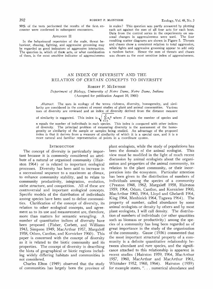
In any series of samples the index value increases as (N), the number of individuals sampled, if they are all of one species (S 1), or as VN if each individual is a new species (S - N). Any intermediate distribution of individuals among species results in a rate of increase falling between these two extremes. Fig. 1 illustrates the increase in index value with increasing numbers of individuals sampled for each of four plant communities, and the theoretical maximum and minimum rates of increase. It is apparent from repeated sampling of artificial and natural communities of varying degrees of homogeneity that increasing the number of individuals sampled is reflected in a nearly linear increase of the index, and the rate of increase (i.e., the slope of the line) is governed by the addition of new species and the way in which the individuals are apportioned among the species.

In artificial communities constructed so that each species had equal numbers of randomly distributed individuals, the increase of index values for samples closely approximated the expected


100 -

L, 80-

D -j

60

Ui2 40 3

LI~~~~~~~

z 20-

4

20 40 60 80 100

NUMBER OF INDIVIDUALS

FIG. 1. Increase of the index iE n2 with increase

in sample size (number of individuals). Line 1. Theoretical maximum (N = 1 species). Line 2. Quarter method sample of temperate hardwood

forest trees (8 species). Line 3. Quadrat sample of a stabilized dune area (15

species). Line 4. Quarter method sample of tropical rainforest

trees (82 species). Line 5. Theoretical minimum. (S = N)

index values. In artificial communities containing a given number of individuals, if the number of species was increased, the rate of increase of the index value (slope of the line) was lowered. If the sample series went from an area with one set of dominants to one with another set of dominants, the rate of increase dropped abruptly pro- ducing a sharp break in the line. If the dominants remained the same but lesser species changed, the break was less conspicuous.

Several sampling techniques were used to ex- amine the relation of numbers of individuals to species and its effect on this index. The most direct method is simply to select a series of random points and note the nearest individual to each point. With this method a sample of 100 individuals (trees only) in a forest community gave an index value of 55.3. A quarter method (Cot- tam and Curtis 1956) on the same population gave a value of 57.8, while a quadrat sample gave 58.8. The value calculated from a total census of the population was 57.2. Five separate stratified random samples of 100 individuals using the quarter method on another forest tree population gave values ranging from 52.5 to 56.8 (mean 54.5). In general, the rates of increase were similar by

point, quarter, or quadrat sampling methods. This was true for random artificial populations and for natural populations including non-random distribution.

It is to be expected that clumping of individuals will result in fewer species being encountered and in a higher index value at any sample size. Quad- rat samples (100 individuals) of an artificial community of 712 individuals and 25 species, all randomly distributed, resulted in an index value of 30.9. If the same species were all closely clumped, the index value was 39.4. This effect is more pronounced if a quadrat sampling technique is used than if a point sampling technique is used.

QUALITATIVE AND QUANTITATIVE DATA

Samples of communities may be compared by simply noting the presence or absence of species (qualitative data), or the species may be weighted by a quantitative measure such as density. If presence and absence data are used, only the richness of the two communities is involved, i.e., the species lists. If a community is maximally diverse (S - N), there is no distinction between qualitative and quantitative data. This suggests that the value of quantitative data in comparing communities diminishes as diversity increases and more species are represented by one or a few individuals. Qualitative data are simply a statement of richness with an assumption of equal density (i.e., all 1) and always imply maximum diversity. The index value of any sample when

S N (i.e., for qualitative data) is VS which is thus the portion attributable to the qualitative component. If quantitative data are used, the portion of the total index attributable to the quan-

titative data of the sample is E i2 -\VS.

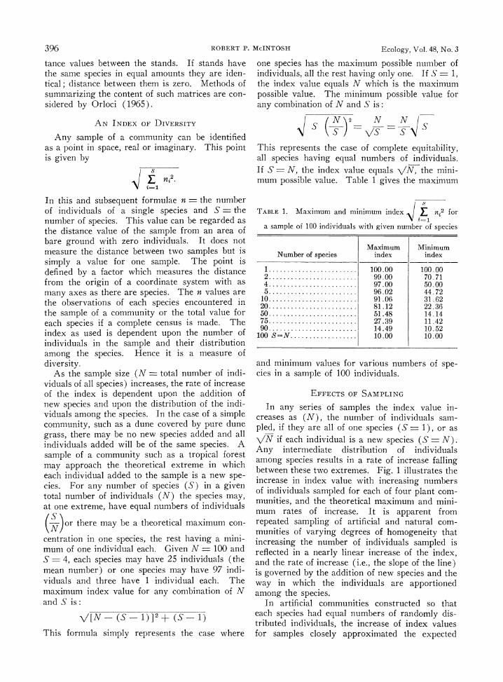
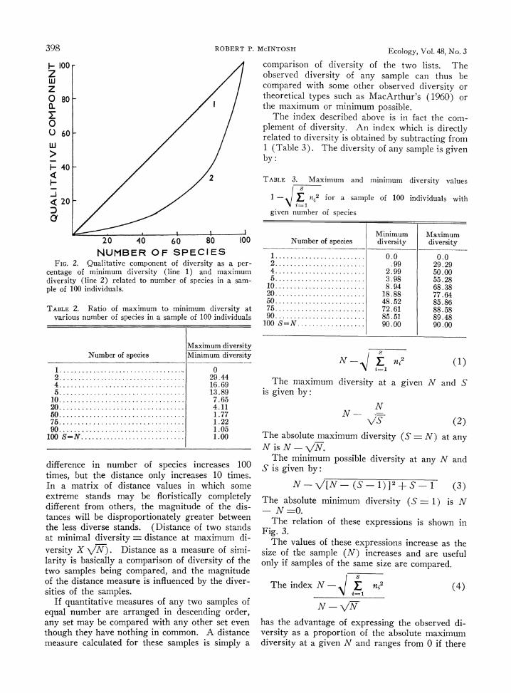
As diversity increases, the fraction of the index attributable to the quantitative component decreases until S = N when it is 0. Conversely, the component attributable to the qualitative component increases until it is 100%. Fig. 2 shows the relation of the qualitative component to the maximum and minimum diversity values respectively. The ratio of minimum to maximum diversity diminishes as the number of species increases and becomes 1 as S - N (Table 2). This simply indicates that the quantitative component of the data becomes less significant as S approaches N.

Qualitative data make diverse samples appear more similar than less diverse samples. If two qualitative samples differ by two species, the distance is V2 = ( 1.414); if the stands differ by

200 species, the distance is V\200 (14.14). The


H_ 100 z uj z 0 80 - I

0 0 60 - U]

H 40 -

_j < 20 -

20 40 60 80 100 NUMBER OF SPECIES

FIG. 2. Qualitative component of diversity as a percentage of minimum diversity (line 1) and maximum diversity (line 2) related to number of species in a sample of 100 individuals.

TABLE 2. Ratio of maximum to minimum diversity at various number of species in a sample of 100 individuals

Maximum diversity Number of species Minimum diversity

1. 0 2.. 29.44 4.. 16.69 5.. 13.89

10 ..7.65 20 ..4.11 50 . .......................... 1.77 75 ..1.22 90 ..1.05

100 S=N. ........................... 1.00

difference in number of species increases 100 times, but the distance only increases 10 times. In a matrix of distance values in which some extreme stands may be floristically completely different from others, the magnitude of the dis- tances will be disproportionately greater between the less diverse stands. (Distance of two stands at minimal diversity = distance at maximum diversity X VN). Distance as a measure of similarity is basically a comparison of diversity of the two samples being compared, and the magnitude of the distance measure is influenced by the diversities of the samples.

If quantitative measures of any two samples of equal number are arranged in descending order, any set may be compared with any other set even though they have nothing in common. A distance measure calculated for these samples is simply a

comparison of diversity of the two lists. The observed diversity of any sample can thus be compared with some other observed diversity or theoretical types such as MacArthur's (1960) or the maximum or minimum possible.

The index described above is in fact the complement of diversity. An index which is directly related to diversity is obtained by subtracting from 1 (Table 3). The diversity of any sample is given by:

TABLE 3. Maximum and minimum diversity values

1 -< E n,2 for a sample of 100 individuals with

given number of species

Minimum Maximum Number of species diversity diversity

1. .................. 0.0 0.0 2...................... .99 29.29 4...................... 2.99 50.00 5...................... 3.98 55.28

10 ..................... 8.94 68.38 20 ..................... 18.88 77.64 50 ..................... 48.52 85.86 75 ..................... 72.61 88.58 90 ..................... 85.51 89.48

100 S=N .................. 90.00 90.00

i:@ E n2 (1) ni2

The maximum diversity at a given N and S is given by:

N N -

V'S (2) The absolute maximum diversity (S = N) at any N is N- VN.

The minimum possible diversity at any N and S is given by:

N-V[N- (S- 1)]2+S 1 (3) The absolute minimum diversity (S 1) is N

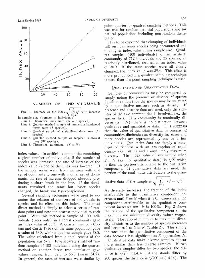
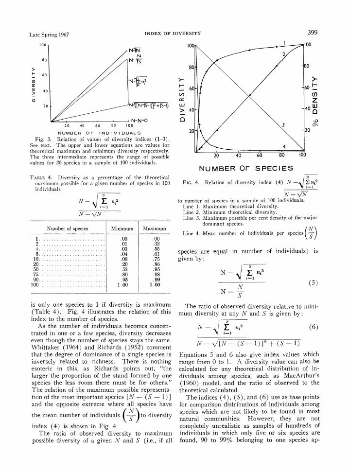
N -0. The relation of these expressions is shown in

Fig. 3. The values of these expressions increase as the

size of the sample (N) increases and are useful only if samples of the same size are compared.

The index N - E 2 (4)

N -VN has the advantage of expressing the observed diversity as a proportion of the absolute maximum diversity at a given N and ranges from 0 if there


100

N

so tN --IS

F- 60

(n N ~n2

0 XINi-1A (S- I) 2 0 N- [N-(S- 1fl2+(S

N-N=O 20 40 60 80 1 00

NUMBER OF IND I VI DUALS

Fig. 3. Relation of values of diversity indices (1-3). See text. The upper and lower equations are values for theoretical maximum and minimum diversity respectively. The three intermediate represents the range of possible values for 20 species in a sample of 100 individuals.

TABLE 4. Diversity as a percentage of the theoretical maximum possible for a given number of species in 100 individuals

N- - E ni2 j=1

Number of species Minimum Maximum

1 ................... .00 .00 2 ............ ....... .01 .32 4 .......... .03 .55 5 ..................... .04 .61

10 .. .09 .75 20 ....................... .20 .86 50 ....................... .53 .95 75 ....................... .80 .98 90 ....................... .95 .99

100 ................. 1.00 1.00

is only one species to 1 if diversity is maximum (Table 4). Fig. 4 illustrates the relation of this index to the number of species.

As the number of individuals becomes concen- trated in one or a few species, diversity decreases even though the number of species stays the same. Whittaker (1964) and Richards (1952) comment that the degree of dominance of a single species is inversely related to richness. There is nothing esoteric in this, as Richards points out, "the larger the proportion of the stand formed by one species the less room there must be for others." The relation of the maximum possible representation of the most important species [N - (S -1) ] and the opposite extreme where all species have

the mean number of individuals ( to diversity

index (4) is shown in Fig. 4. The ratio of observed diversity to maximum

possible diversity of a given N and S (i.e., if all

100 I 100

2

80 80

- 60, 6

V)~~~~~~~~~~~~~U Q~~~~~ ~~z

LU i > 4. 40 4)

30

20- -20

4

20 40 60 80 00

NUMBER OF SPECIES

FIG. 4. Relation of diversity index (4) N -\I2n2

to number of species in a sample of 100 individuals. Line 1. Maximum theoretical diversity. Line 2. Minimum theoretical diversity. Line 3. Maximum possible per cent density of the major

dominant species.

Line 4. Mean number of individuals per species (i-)

species are equal in number of individuals) is given by:

N < E 2(5) N -N

The ratio of observed diversity relative to minimum diversity at any N and S is given by:

N < t is2 (6)

N-V[N-(S 1)]2+ (S-i)

Equations 5 and 6 also give index values which range from 0 to 1. A diversity value can also be calculated for any theoretical distribution of individuals among species, such as MacArthur's (1960) model, and the ratio of observed to the theoretical calculated.

The indices (4), (5), and (6) use as base points for comparison distributions of individuals among species which are not likely to be found in most natural communities. However, they are not completely unrealistic as samples of hundreds of individuals in which only five or six species are found, 90 to 99% belonging to one species ap-


proach the condition of theoretical minimum possible diversity (Frolik 1941, Hanson 1951). Cer- tain types of rain forest produce samples of hundreds of species most represented by one or a few individuals and none having more than 5% of the total (Poore 1964), a situation approaching the theoretical maximum diversity.

DIVERSITY AND DISTANCE

Two stands (A and B) which are completely different having no species in common will have a distance equal to

nA + ? nB2.

If A and B each have only one species the distance value will be

N/NA + NB2.

A third stand C which has no species in common with A or B but which is maximally diverse will have a distance from A equal to

NA2 + EtC2-

If sampled by the same N, stand C will be closer, as measured by distance, to A than B is to A. Thus a very diverse stand will appear more similar to a less diverse stand than to another less diverse stand. This is due simply to the fact that a given quantity (individual) has a greater impact on the distance value in a species represented by other individuals than if the individual is the first of a new species. The reverse is true of the effect of an individual on diversity, i.e., its effect is maximum if it is the first representing a new species and becomes progressively less if it is simply one more of a species already represented by other individuals.

COMPARISONS OF INDICES OF DIVERSITY

Several indices of diversity have been proposed (Whittaker 1964). Some of these are predicated upon hypotheses about the distribution of numbers of individuals among species and are not considered here. Several are independent of a theory about the distribution of individuals among species and are compared here with the index discussed above.

One, derived from information theory, which has been widely used in recent work of animal ecologists is discussed in detail by Margaleff (1958) and used by Hairston (1959), MacArthur and MacArthur (1961), Patten (1962), and Lloyd and Ghelardi (1964). This index is

S

D E Pr log, Pr. = =1

Hairston and MacArthur and MacArthur give the formula with natural logarithms. Lloyd and Ghelardi use the logarithm to the base 2. The results are in different units. If the natural logarithm is used the resulting unit is called the nat; if the logarithm to the base 2 is used the unit is called the bit. Pr is the proportion of the individual species of the density per cent. In the notation used here this equation is:

s ni - ~log, I N l~eN

Clarification of this index can be found in Ashby (1956) or Abramson (1963). This value is the sum of the proportions of the individual species multiplied by the negative logarithm of the proportion. It ranges from 0 (loge of 1), if all of thl,. individuals are of one species to loge N, if the number of species equals the number of individuals. The index is maximum for any S if all species have equal numbers of individuals and minimum if the individuals are maximally con- centrated in one species. Table 5 gives the maxi-

TABLE 5. Maximum and minimum values of information theory diversity index for a sample of 100 individuals with given number of species

Number of species Minimum Maximum diversity diversity

1.0................... 0 2 ....................... 0.69 0.06 4 ....................... 1.38 .17 5 ....................... 1.60 .23

10 ....................... 2.30 .50 20 ....................... 2.98 1.04 50 ....................... 3.90 2.60 75 ....................... 4.20 3.75 90 ....................... 4.41 4.34

100 ....................... 4.60 4.60

mum and minimum values for this index in a population of 100 individuals at various numbers of species. This index is a measure of information in a group of objects (species) which have different probabilities of being represented, i.e., numbers of individuals. Information is maximum when the probabilities (densities) of all species are equal. It is then equal to the loge S. Infor- mation is 0 if there is only one possibility, i.e., diversity is 0.

The ecologist commonly identifies a number of organisms in sequence as he encounters them in a series of samples. Each additional individual adds to his view of the community. It is a com- monplace that an adequate representation of a


poor community is gained after only a few individuals have been recorded, while a rich and diverse community requires examination of more individuals. Normally the ecologist is not concerned about the precise sequence or position of each individual in the series, but his data often include the number of individuals of each species. The total amount of information is determined by the number of individuals and the species encountered. It is maximum if each individual be- longs to a different species and diminishes as the individuals are grouped into fewer species, being minimum if all individuals are of the same species. This diminution of information is due to the redundancy or repetition of individuals of the same species. As the number of individuals increases, fewer new species are found, and the new individuals added are more of those previously seen, roughly in proportion to their density in the community, i.e., redundancy increases. Fig. 5

22 100

><80/ - -

601 0 I /

w201 > I

20 40 60 80 100

NUMBER OF SP E CIE S FIG. 5. Comparison of distributions of the maximum

and minimum diversity values of three diversity indices. The lower three lines are the minimum values, the upper three the maximum.

Solid line-Information theory - n loge n N Nj

Dash line-Complement of Simpson's Index 1 - (n) Dash-dot line-Diversity index (4) N- - (n,)2

N-VN

illustrates the distribution of this index in a sample of 100 individuals. It is calculated as a percentage of the maximum for comparison with the other indices shown.

Simpson's (1949) index is the sum of the squares of the proportions of the component spe-

S S n2 cies Pr2 or, in the notation used here ?

1 N

It ranges from 1 if all of the individuals are of

one species to (+) if they are equally divided

among the species (S). It approaches 0 as S -- N and as S increases. It is the inverse of diversity; its complement is directly related to diversity. Table 6 gives values for Simpson's index and Fig.

TABLE 6. Values of Simpson's index for 100 N at various numbers of species

Number of species Minimum Maximum diversity diversity

1 ..................... 1.00 1.00 2 ....................... .98 .50 4 ....................... .94 .25 5 ....................... .92 .20

10 ....................... .83 .10 20 ....................... .66 .05 50 ....................... .26 .02 75 ....................... .075 .013 90 ....................... .021 .011

100 ....................... .010 .010

al-Simpson's index converts to direct relation to diversity.

5 shows its distribution as compared to the indices already discussed. An estimate of the true population figure for this index is given by

n- (n- 1) N(N -1)

according to Simpson (1949) and Greig-Smith (1964). Williams (1964) inverts this so that the increase in the value is directly related to diversity.

DIsCUSSION

R. W. Gerard (1965) comments: "Before measurements can be meaningful they must be directed to the right things and, even in science, finding these things is the major achievement; entitation is more important than quantitation." Herein lies a major difficulty of ecology. Measurements of community properties such as diversity, stability, or productivity are enlightening only when the entity in which they are made is meaningful. The traditional belief, particularly among plant ecologists (phytosociologists), in the existence of a homogeneous community as an organic entity discernible to the practiced eye of the ecologist is currently much in dispute. Yet it remains as an axiom in many current ecological studies. Beyers (1963), for example, begins a paper with an open- ing sentence: "The flora and fauna of the earth


are grouped into communities which have a definite structure and organization." If this were true, measurements of diversity and other properties could be readily made and referred to the appropriate communities. However, the much vexed question of the nature, definition, and recognition of communities of organisms is still very much with us. Community definitions range from explicit statements about the community and its properties to studious avoidance of any definition.

Recent developments in quantitative technique indicate that these may be useful in circumscribing entities or communities as well as in providing quantitative analytic data on subjectively determined entities. The development of effective rapid sampling methods coupled with increasing availa- bility of computing facilities makes possible re- fined methods of quantitative analysis and techniques for limiting heterogeneity or specifying its degree. Entities, as Gerard notes, are dissected from their surroundings and the ecologist calls them variously, stands, samples, communities, or associations. How these are dissected and what is dissected is of extreme importance, and the need for effective objective means of delineating, describing, and comparing representative samples of groups of organisms is pressing. Poore (1964) notes the need for adequate measures of uniformity (homogeneity), diversity, and size of pattern, all of which are important aspects of the assessment of the community. At the present time quantitation in the sense of analytic methods is well developed; entitation in the sense of objective and quantitative synthetic methods is poorly developed. There is poor integration between the work of plant ecologists, the long time students of the community and its properties, and that of animal ecologists who lately are empha- sizing community studies. Both, as noted in the introduction, share the same essential problems, and use similar concepts, terminology, and techniques. Confusion and unnecessary duplication of effort have resulted from the failure to recognize the common ground in concept and technique and, as usual, from overlapping or contradictory terminology. Some of the most interesting and important problems facing the ecologist will not be adequately approached until the critical problem of entitation is resolved. It does not follow that this requires a commitment to a particular system of classification or even a belief that classes exist. It is quite possible to regard the distribution of organisms as continuous and best studied by ordination techniques with the entities simply being objectively delimited segments of the continuum.

Margaleff (1958) points out that the study of homogeneity cannot be separated from the deter-

mination of "biocoenotic units," and indeed this remains the crux of the problem. If diversity is a property of a homogeneous community, the community must be identified and described and its homogeneity verified. If it is asserted to be homogeneous, either as a concrete instance in space or as an abstract entity, this should be demonstrated by appropriate tests in addition to demonstrating that its diversity approximates a theoretical model. Since it is generally agreed that strict homogeneity in the statistical sense is not likely to be found in any natural community, diversity must be assessed in respect to some defined limits of heterogeneity or dissimilarity rather than a putative homogeneity.

This problem is approached by Whittaker (1960) in recognizing three types of diversity. One, measured by Williams' (1964) "alpha" index of diversity, is the diversity of a single stand or community. This implies a degree of homogeneity in the stand studied. The second, "beta diversity," is the extent of change of community composition on a gradient of environment which includes considerably different communities. This is the type of difference which is commonly measured by similarity indices. Whittaker suggests as a measure of beta diversity a ratio of the Wil- liams' "alpha" value of the merged samples on the "coenocline" to the "alpha" of an individual sample. Alternatively he suggests a measure of stand or sample similarity related to the distance on the ground between the stands. Beta diversity is something like "heterogeneously diverse" of Hutchinson (1958) as described earlier in this paper. The third "gamma diversity" is the diversity of a number of samples of a community taken from a range of environments. It is measured by simple richness or by Williams' alpha index of diversity and presumably is a resultant of alpha and beta diversities.

Alpha, beta, and gamma diversities as described by Whittaker each incorporate a degree of heterogeneity. It is difficult to dissociate beta from gamma diversity and both are clearly dependent upon the range of variation which is included. Beta diversity approaches the use of diversity when it is applied to a geographic area including a wide range of habitats. It is clear that some way of specifying the range of community dif- ferentiation included, i.e., the degree of heterogeneity, is necessary to make the concept of diversity of maximum use in ecological studies. The entity and its scope must be made clear before the measure of diversity takes on useful meaning. The concept of diversity then has limited use in ecological studies in the absence of a clear indica-

Late SDring 1967 INDEX OF DIVERSITY 403 tion of the homogeneity of the samples or community in which the diversity is measured.

It is clear from Fig. 5 that the three indices of diversity considered here have similar distributions. There is no apparent reason why any one of these should be a priori correct. The diversity

indices based on the value J ni2 are derived

from the distance formula which essentially com- pares the diversity of two samples. This index is a special case of the distance measure. It has the advantage of representing data as points in a familiar metric space and in the same coordinate system as distance. Distance is a measure of similarity and is, in effect, a basis for entitation. The diversity index attempts to represent an important property of the entity, the community of organisms.

ACkNOWLEDGMENTS

The author is indebted to Drs. Peter Greig-Smith and Lazlo Orloci and Mr. Michael Austin for directing his attention to the problem of diversity and for many stimu- lating discussions. Appreciation is also expressed to Drs. Michael Levin, Thomas Griffing, Grant Cottam, Glenn Goff, Richard Otter, and Mr. George Hoffman for valuable comments. Much of the work was done during the tenure of a National Science Foundation Faculty Fellowship at the University College of North Wales, Bangor, Caerns.

LITERATURE CITED

Abramson, N. 1963. Information theory and coding. McGraw-Hill Book Co., New York. 201 p.

Ashby, W. R. 1956. An introduction to cybernetics. Chapman and Hall Ltd., London. 295 p.

Audy, J. R. 1948. Some ecological affects of defores- tation and settlement. Malay Nat. J. 3: 178-189.

Austin, M. P., and L. Orloci. 1966. An evaluation of some ordination techniques. J. Ecol. 54: 217-227.

Becking, R. W. 1957. The Zurich-Montpellier school of phytosociology. Bot. Rev. 22: 441-489.

Beckner, M. 1959. The biological way of thought. Columbia Univ. Press, New York. 200 p.

Beyers, R. J. 1963. The metabolism of twelve aquatic laboratory ecosystems. Ecol. Monogr. 33: 281-306.

Black, G. A., Th. Dobzhansky, and C. Pavan. 1950. Some attempts to estimate species diversity and population diversity of trees in Amazonian forests. Bot. Gaz. 111: 413-425.

Bray, J. R., and J. T. Curtis. 1957. An ordination of the upland forest communities of Southern Wiscon- sin. Ecol. Monogr. 27: 325-349.

Catana, A., Jr. 1964. A distribution free method for the determination of homogeneity in distance data. Ecology 45: 640-641.

Connell, J. H., and E. Orias. 1964. The ecological regulation of species diversity. Amer. Natur. 48: 399-414.

Cottam, G., and J. T. Curtis. 1956. The use of distance measures in phytosociological sampling. Ecol- ogy 37: 451-460.

Curtis, J. T. 1959. The vegetation of Wisconsin. Univ. of Wisconsin Press, Madison, Wisc. 657 p.

Curtis, J. T., and R. P. McIntosh. 1950. The interre- lations of certain analytic and synthetic photosocio- logical characters. Ecology 31: 434-455.

. 1951. An upland forest continuum in the prairie-forest border region of Wisconsin. Ecology 32: 479-496.

Dahl, E. 1956. Rondane mountain vegetation in South Norway. W. Nygaard, Oslo. 374 p.

. 1960. Some measures of uniformity in vegetation analysis. Ecology 41: 805-808.

Dice, L. R. 1952. Natural communities. University of Michigan Press, Ann Arbor, Mich. 547 p.

Elton, C. 1949. Population interspersion: an essay on animal community studies. J. Ecol. 37: 1-23.

Fisher, R. A., A. S. Corbett, and C. B. Williams. 1943. The relation between number of species and the number of individuals in a random sample from an animal population. J. Anim. Ecol. 12: 42-58.

Frolik, A. L. 1941. Vegetation on the peatlands of Dane County Wisconsin. Ecol. Monogr. 11: 118-140.

Gause, G. F. 1936. Principles of biocoenology. Quart. Rev. Biol. 11: 320-336.

Gerard, R. W. 1965. Intelligence, information and education. Science 148: 762-765.

Goodall, D. W. 1952. Quantitative aspects of plant distribution. Biol. Rev. 27: 194-245.

- . 1954. Vegetational classification and vegetational continua. Angew. Pflansoz. 1: 168-182.

. 1963. The continuum and the individualistic association. Vegetatio 11: 297-316.

Greig-Smith, P. 1964. Quantitative plant ecology. Butterworths, London. 256 p.

Hairston, N. G. 1959. Species abundance and community organization. Ecology 40: 404-416.

. 1964. Studies on the organization of animal communities. Jubilee Symposium Supplement. J. Ecol. 52: 227-239.

Hanson, H. C. 1951. Characteristics of some grass- land, marsh and other plant communities in Western Alaska. J. Ecol. 21: 317-375.

Hutchinson, G. E. 1953. The concept of pattern in ecology. Proc. Acad. Nat. Sci. Philadelphia 105: 1-12.

. 1958. Concluding remarks. Symposium on Quantitative Biology 22: 415-427.

Kershaw, K. A. 1961. Association and covariance analysis of plant communities. J. Ecol. 49: 643-654.

King, C. E. 1962. Some aspects of the ecology of psammolittoral nematodes in the northeastern Gulf of Mexico. Ecology 43: 515-523.

- . 1964. Relative abundance of species and Mac- Arthur's model. Ecology 45: 716-727.

Klopfer, P. H. 1962. Behavioral aspects of ecology. Prentice-Hall, Englewood Cliffs, N. J. 166 p.

Koch, L. F. 1957. Index of biotal dispersity. Ecology 38: 145-148.

Kohn, A. J. 1959. The ecology of Comis in Hawaii. Ecol. Monogr. 29: 47-90.

Lambert, J. M., and M. Dale. 1965. The use of sta- stistics in ecology. Advances in Ecology 2: 59-99.

Lloyd, M., and R. J. Ghelardi. 1964. A table for cal- culating the equitability component of species diversity. J. Anim. Ecol. 33: 217-225.

MacArthur, R. H. 1957. On the relative abundance of bird species. Proc. Nat. Acad. Sci. U.S. 43: 293- 295.

1960. On the relative abundance of species. Amer. Natur. 94: 25-36.

404 FREDERICK R. GEHLBACH Ecology, Vol. 48, No. 3

* 1964. Environmental factors affecting bird species diversity. Amer. Natur. 48: 387-397.

MacArthur, R. H., and J. W. MacArthur. 1961. On bird species diversity. Ecology 42: 594l598.

Macfayden, A. 1954. The invertebrate fauna of Jan Mayen Island E. Greenland. J. Anim. Ecol. 23: 261- 297.

. 1957. Animal ecology. Pitman and Sons, London. 264 p.

Margaleff, D. R. 1958. Information theory in ecology. Yearbook of the Society for General Systems Re- search. Vol. 3. 36-71.

Martin, A. R. H. 1960. The ecology of Groenvlei, a south African fen. J. Ecol. 48: 307-329.

McIntosh, R. P. 1962. Raunkiaer's law of frequency. Ecology 43: 533-535.

McVean, D. N., and D. A. Ratcliffe. 1962. Plant communities of the Scottish Highlands. H. M. Stationery Office, London. 445 p.

Menhinick, E. F. 1964. A comparison of some species- individuals diversity indices applied to samples of field insects. Ecology 45: 859-861.

Meyers, E., and V. J. Chapman. 1953. Statistical analysis applied to a vegetation type in New Zealand. Ecology 34: 175-185.

Newbould, P. J. 1960. The ecology of Cranesmoor, a New Forest valley bog. J. Ecol. 48: 361-383.

Odum, E. P. 1950. Bird populations of the Highlands (N. Carolina) plateau in relation to plant succession and avian invasion. Ecology 31: 587-605.

Odum, H. T., J. E. Cantlon, and J. S. Kornicker. 1960. An organizational hierarchy for the interpretation of species-individual distribution, species entropy, ecosystem evolution and the meaning of a species variety index. Ecology 41: 395-399.

Orloci, L. 1965. Geometric models in ecology. I. The theory and application of some ordination methods. J. Ecol. 54: 193-215.

Park, 0. 1941. Concerning community symmetry. Ecology 22: 164-167.

Patten, B. C. 1962. Species diversity in net phyto- plankton of Raritan Bay. J. Mar. Res. 20: 57-75.

Poore, M. E. D. 1964. Integration in the plant community. J. Ecol. 52 (Supplement): 213-225.

Preston, F. 1948. The commonness, and rarity, of species. Ecology 29: 254-283.

. 1962. The canonical distribution of commonness and rarity. I. Ecology 43: 185-216. II. Ecol- ogy 43: 410-432.

Raisbeck, G. 1964. Information theory. An introduction for scientists and engineers. M.I.T. Press, Cam- bridge, Mass. 105 p.

Richards, P. W. 1952. The tropical rain forest. Cam- bridge Univ. Press, Cambridge, Mass. 450 p.

Simpson, E. H. 1949. Measurement of diversity. Na- ture 163: 688.

Sokal, R. R. 1961. Distance as a measure of taxonomic similarity. Syst. Zool. 10: 71-79.

Sokal, R. R., and P. H. A. Sneath. 1963. Principles of numerical taxonomy. W. H. Freeman Co., San Francisco, Calif. 359 p.

Tagawa, Hideo. 1964. A study of the volcanic vegetation in Sukurajima, Southwest Japan. Mem. Fac. Sci. Kyushu Univ. Ser. E. 3: 165-228.

Turner, F. B. 1961. The relative abundance of snake species. Ecology 42: 600-603.

Watt, A. S. 1964. The community and the individual. J. Ecol. 52 (Supplement): 203-211.

Whittaker, R. H. 1952. A study of summer foliage insect communities in the Great Smoky Mountains. Ecol. Monogr. 22: 1-44.

. 1960. Vegetation of the Siskiyou Mountains, Oregon and California. Ecol. Monogr. 30: 279-338.

. 1964. Dominance and diversity in land plant communities. Science 147: 250-260.

Williams, C. B. 1964. Patterns in the balance of nature. Academic Press, London. 324 p.

Williams, W. T., and J.. Lambert. 1959. Multivariate methods in plant ecology. I. Association analysis in plant communities. J. Ecol. 47: 83-101.

. 1961. Multivariate methods in plant ecology. III. Inverse association-analysis. J. Ecol. 49: 717- 729.

VEGETATION OF THE GUADALUPE ESCARPMENT, NEW MEXICO-TEXAS

FREDERICK R. GEHLBACH

Department of Biology, Baylor University, Waco, Texas (Accepted for publication January 20, 1967)

Abstract. The Guadalupe Escarpment, a Permian limestone reef, is the eastern face of a semiarid-mesothermal mountain mass that rises 1,000-4,000 ft above the southwestern edge of the Great Plains. Phytocenoses range from xerophytic (Larrea, Flourensia, Acacia dominance types) on the silty to gravelly plains, through less xerophytic (Agave, Dasylirion, Juniperus dominance types) on gravelly to bouldery lower slopes, to comparatively mesophytic (funiperus, Quercus, Pinus dominance types) on rocky upper slopes and the escarpment peneplain. This general gradient is a vegetational continuum in which species' ecologic ampli- tudes are distinct but form overlapping assemblages of similar structure.

Special environmental gradients are produced by topographic discontinuity. On low eleva- tion canyon slopes, south-facing exposures support more xerophytic dominance types than north-facing exposures, although floristic differences are minimal. At highest base levels and slope elevations, south-facing exposures support the most xerophytic of all canyonside vegetation, and floristic differences between slopes are maximal. Dominance types with a tree stratum are well developed inside canyons; they form a continuous streambed-stream terrace-

an index of diversity and the relation of certain concepts ...(margaleff 1958, macarthur and...

Documents