an integratable v-x communication based conventional
TRANSCRIPT

An Integratable V-X Communication based Conventional Vehicle Fuel Optimization modelfor distance based Ecological Driving Scheme
by
Prudhvi Raj Rongali
A thesis submitted in partial fulfillmentof the requirements for the degree of
Master of Science in Engineering(Computer Engineering)
in the University of Michigan-Dearborn2018
Master’s Thesis Committee:
Assistant Professor Wencong Su, ChairAssistant Professor Mengqi WangAssistant Professor Riadul Islam

ACKNOWLEDGEMENTS
First and foremost I wish to thank my advisor, Dr. Wencong Su, Assistant Professor in the De-
partment of Electrical and Computer Engineering. Whose guidance, support and encouragement
from the initial to the final level of completion of my Thesis work.
Finally, I must express my very profound gratitude to my parents for providing me with unfail-
ing support and continuous encouragement throughout my years of study. This accomplishment
would not have been possible without them. Thank you.
ii

TABLE OF CONTENTS
ACKNOWLEDGEMENTS . . . . . . . . . . . . . . . . . . . . . . . . . . . . . . . . ii
LIST OF FIGURES . . . . . . . . . . . . . . . . . . . . . . . . . . . . . . . . . . . . v
ABSTRACT . . . . . . . . . . . . . . . . . . . . . . . . . . . . . . . . . . . . . . . . . viii
CHAPTER
I. Introduction . . . . . . . . . . . . . . . . . . . . . . . . . . . . . . . . . . . . . 1
1.1 Context . . . . . . . . . . . . . . . . . . . . . . . . . . . . . . . . . . . . 51.1.1 Definitions . . . . . . . . . . . . . . . . . . . . . . . . . . . . 5
1.2 Eco-driving . . . . . . . . . . . . . . . . . . . . . . . . . . . . . . . . . 5
II. Vehicle and SPAT model . . . . . . . . . . . . . . . . . . . . . . . . . . . . . . 6
2.1 Vehicle Model . . . . . . . . . . . . . . . . . . . . . . . . . . . . . . . . 62.2 SPAT Model . . . . . . . . . . . . . . . . . . . . . . . . . . . . . . . . . 9
III. Optimization problem . . . . . . . . . . . . . . . . . . . . . . . . . . . . . . . 14
3.1 Cross window search and Adjacency matrix creation Algorithm . . . . . 153.2 Adjacency matrix and graph reduction . . . . . . . . . . . . . . . . . . . 173.3 Optimal path . . . . . . . . . . . . . . . . . . . . . . . . . . . . . . . . . 18
IV. Integration of ”nonstop” model to distance based long term optimization . . . 25
4.1 Distance based Eco driving scheme long term optimization . . . . . . . . 254.2 Simulation and Results . . . . . . . . . . . . . . . . . . . . . . . . . . . 27
4.2.1 Standalone Simulation Results of proposed model: . . . . . . . 284.2.2 Simulation results when the v target (k + 1) is fed with above
optimal speed profile: . . . . . . . . . . . . . . . . . . . . . . . 284.2.3 Case Studies . . . . . . . . . . . . . . . . . . . . . . . . . . . 304.2.4 Case:1 . . . . . . . . . . . . . . . . . . . . . . . . . . . . . . . 304.2.5 Case:2 . . . . . . . . . . . . . . . . . . . . . . . . . . . . . . . 364.2.6 Case:3 . . . . . . . . . . . . . . . . . . . . . . . . . . . . . . . 43
iii

BIBLIOGRAPHY . . . . . . . . . . . . . . . . . . . . . . . . . . . . . . . . . . . . . 51
iv

LIST OF FIGURES
Figure
1.1 EU green house gases emission trends, projections. . . . . . . . . . . . . . . . . 11.2 Fuel consumption vs. cruise speed. . . . . . . . . . . . . . . . . . . . . . . . . 21.3 An idealized time-distance diagram showing signal co-ordination with a fixed
time plan. . . . . . . . . . . . . . . . . . . . . . . . . . . . . . . . . . . . . . . 31.4 Example of urban traffic environment. . . . . . . . . . . . . . . . . . . . . . . . 41.5 V2I communication in urban traffic environment. . . . . . . . . . . . . . . . . . 42.1 Fuel rate vs Torque. . . . . . . . . . . . . . . . . . . . . . . . . . . . . . . . . . 72.2 Fuel rate vs Engine speed. . . . . . . . . . . . . . . . . . . . . . . . . . . . . . 72.3 Fuel map. . . . . . . . . . . . . . . . . . . . . . . . . . . . . . . . . . . . . . . 82.4 Signal status for Traffic light 1. . . . . . . . . . . . . . . . . . . . . . . . . . . . 102.5 Signal status for Traffic light 2. . . . . . . . . . . . . . . . . . . . . . . . . . . . 102.6 Signal status for Traffic light 3. . . . . . . . . . . . . . . . . . . . . . . . . . . . 112.7 Signal status for Traffic light 4. . . . . . . . . . . . . . . . . . . . . . . . . . . . 112.8 Signal status for Traffic light 5. . . . . . . . . . . . . . . . . . . . . . . . . . . . 122.9 Signal status for Traffic light 6. . . . . . . . . . . . . . . . . . . . . . . . . . . . 122.10 Vehicle passing through traffic intersection during Green phase. . . . . . . . . . . 133.1 Crossing window algorithm. . . . . . . . . . . . . . . . . . . . . . . . . . . . . 143.2 Crossing window for Traffic light 1. x-axis: time(sec), y-axis:signal status(1 or 0). 193.3 Crossing window for Traffic light 2. x-axis: time(sec), y-axis:signal status(1 or 0). 193.4 Crossing window for Traffic light 3. x-axis: time(sec), y-axis:signal status(1 or 0). 193.5 Crossing window for Traffic light 4. x-axis: time(sec), y-axis:signal status(1 or 0). 203.6 Crossing window for Traffic light 5. x-axis: time(sec), y-axis:signal status(1 or 0). 203.7 Crossing window for Traffic light 6. x-axis: time(sec), y-axis:signal status(1 or 0). 203.8 tmin crossing point for Traffic light 1. . . . . . . . . . . . . . . . . . . . . . . . . 213.9 tmax crossing point for Traffic light 1. . . . . . . . . . . . . . . . . . . . . . . . 213.10 Vehicle trajectory through green crossing windows. . . . . . . . . . . . . . . . . 223.11 Node structure for Dijkstra algorithm. . . . . . . . . . . . . . . . . . . . . . . . 233.12 Adjacency Matrix. . . . . . . . . . . . . . . . . . . . . . . . . . . . . . . . . . . 233.13 Directed graph with fuel weights. . . . . . . . . . . . . . . . . . . . . . . . . . . 244.1 Two-Stage Ecological Driving Scheme. . . . . . . . . . . . . . . . . . . . . . . 264.2 speed and time profile. . . . . . . . . . . . . . . . . . . . . . . . . . . . . . . . 294.3 torque and brake profile. . . . . . . . . . . . . . . . . . . . . . . . . . . . . . . 294.4 Case1 Crossing window for Traffic light 1. x-axis: time(sec), y-axis:signal sta-
tus(1 or 0). . . . . . . . . . . . . . . . . . . . . . . . . . . . . . . . . . . . . . . 30
v
4.5 Case1 Crossing window for Traffic light 2. x-axis: time(sec), y-axis:signal sta-tus(1 or 0). . . . . . . . . . . . . . . . . . . . . . . . . . . . . . . . . . . . . . . 31
4.6 Case1 Crossing window for Traffic light 3. x-axis: time(sec), y-axis:signal sta-tus(1 or 0). . . . . . . . . . . . . . . . . . . . . . . . . . . . . . . . . . . . . . . 31
4.7 Case1 Crossing window for Traffic light 4. x-axis: time(sec), y-axis:signal sta-tus(1 or 0). . . . . . . . . . . . . . . . . . . . . . . . . . . . . . . . . . . . . . . 31
4.8 Case1 Crossing window for Traffic light 5. x-axis: time(sec), y-axis:signal sta-tus(1 or 0). . . . . . . . . . . . . . . . . . . . . . . . . . . . . . . . . . . . . . . 32
4.9 Case1 Crossing window for Traffic light 6. x-axis: time(sec), y-axis:signal sta-tus(1 or 0). . . . . . . . . . . . . . . . . . . . . . . . . . . . . . . . . . . . . . . 32
4.10 Case1 Vehicle trajectory through green crossing windows. . . . . . . . . . . . . 324.11 Case1 Node structure for Dijkstra algorithm. . . . . . . . . . . . . . . . . . . . . 334.12 Case1 Adjacency Matrix. . . . . . . . . . . . . . . . . . . . . . . . . . . . . . . 334.13 Case1 Directed graph with fuel weights. . . . . . . . . . . . . . . . . . . . . . . 344.14 Case1 speed and time profile. . . . . . . . . . . . . . . . . . . . . . . . . . . . . 354.15 Case1 torque and brake profile. . . . . . . . . . . . . . . . . . . . . . . . . . . . 364.16 Case2 Crossing window for Traffic light 1. x-axis: time(sec), y-axis:signal sta-
tus(1 or 0). . . . . . . . . . . . . . . . . . . . . . . . . . . . . . . . . . . . . . . 374.17 Case2 Crossing window for Traffic light 2. x-axis: time(sec), y-axis:signal sta-
tus(1 or 0). . . . . . . . . . . . . . . . . . . . . . . . . . . . . . . . . . . . . . . 374.18 Case2 Crossing window for Traffic light 3. x-axis: time(sec), y-axis:signal sta-
tus(1 or 0). . . . . . . . . . . . . . . . . . . . . . . . . . . . . . . . . . . . . . . 384.19 Case2 Crossing window for Traffic light 4. x-axis: time(sec), y-axis:signal sta-
tus(1 or 0). . . . . . . . . . . . . . . . . . . . . . . . . . . . . . . . . . . . . . . 384.20 Case2 Crossing window for Traffic light 5. x-axis: time(sec), y-axis:signal sta-
tus(1 or 0). . . . . . . . . . . . . . . . . . . . . . . . . . . . . . . . . . . . . . . 384.21 Case2 Crossing window for Traffic light 6. x-axis: time(sec), y-axis:signal sta-
tus(1 or 0). . . . . . . . . . . . . . . . . . . . . . . . . . . . . . . . . . . . . . . 394.22 Case2 Vehicle trajectory through green crossing windows. . . . . . . . . . . . . 394.23 Case2 Node structure for Dijkstra algorithm. . . . . . . . . . . . . . . . . . . . . 404.24 Case2 Adjacency Matrix. . . . . . . . . . . . . . . . . . . . . . . . . . . . . . . 404.25 Case2 Directed graph with fuel weights. . . . . . . . . . . . . . . . . . . . . . . 414.26 Case2 speed and time profile. . . . . . . . . . . . . . . . . . . . . . . . . . . . . 424.27 Case2 torque and brake profile. . . . . . . . . . . . . . . . . . . . . . . . . . . . 434.28 Case3 Crossing window for Traffic light 1. x-axis: time(sec), y-axis:signal sta-
tus(1 or 0). . . . . . . . . . . . . . . . . . . . . . . . . . . . . . . . . . . . . . . 444.29 Case3 Crossing window for Traffic light 2. x-axis: time(sec), y-axis:signal sta-
tus(1 or 0). . . . . . . . . . . . . . . . . . . . . . . . . . . . . . . . . . . . . . . 444.30 Case3 Crossing window for Traffic light 3. x-axis: time(sec), y-axis:signal sta-
tus(1 or 0). . . . . . . . . . . . . . . . . . . . . . . . . . . . . . . . . . . . . . . 454.31 Case3 Crossing window for Traffic light 4. x-axis: time(sec), y-axis:signal sta-
tus(1 or 0). . . . . . . . . . . . . . . . . . . . . . . . . . . . . . . . . . . . . . . 454.32 Case3 Crossing window for Traffic light 5. x-axis: time(sec), y-axis:signal sta-
tus(1 or 0). . . . . . . . . . . . . . . . . . . . . . . . . . . . . . . . . . . . . . . 45
vi
4.33 Case3 Crossing window for Traffic light 6. x-axis: time(sec), y-axis:signal sta-tus(1 or 0). . . . . . . . . . . . . . . . . . . . . . . . . . . . . . . . . . . . . . . 46
4.34 Case3 Vehicle trajectory through green crossing windows. . . . . . . . . . . . . 464.35 Case3 Node structure for Dijkstra algorithm. . . . . . . . . . . . . . . . . . . . . 474.36 Case3 Adjacency Matrix. . . . . . . . . . . . . . . . . . . . . . . . . . . . . . . 474.37 Case3 Directed graph with fuel weights. . . . . . . . . . . . . . . . . . . . . . . 484.38 Case3 speed and time profile. . . . . . . . . . . . . . . . . . . . . . . . . . . . . 494.39 Case3 torque and brake profile. . . . . . . . . . . . . . . . . . . . . . . . . . . . 50
vii
ABSTRACT
This thesis paper proposes An Integratable V-X Communication-based Conventional Vehicle
Fuel Optimization model for real-time traffic conditions. Before departure, the speed profile for
an entire route is optimized using signal phase and timing (SPAT ) information and location of
traffic lights to provide smooth transitions at traffic signal intersections. In this study, we are going
to develop ”nonstop” optimal speed model that can be integrated to existing distance based eco-
driving schemes. The initial simulation is done using MATLAB to evaluate optimal speed, fuel
economy, the travel time of the ”nonstop” model and the results are compared with the optimization
results from distance based eco-driving scheme which uses an estimation of distribution algorithm
(EDA). Further integration compatibility of ”nonstop” model with the distance based eco-driving
scheme is analyzed.
viii

CHAPTER I
Introduction
Energy consumption optimization and pollution reduction are increasingly becoming critical.
For the past decade the number of vehicles on road are increasing exponentially. This lead to
serious debate in developing vehicle optimization techniques to cut the emissions. The European
Union passed the legislation to cut the emissions by 20 percent towards the end of 2020 [1]. The
figure 1.1 describes the projections and targets in the EU by 2020 and beyond.
Figure 1.1: EU green house gases emission trends, projections[1].
This similar trend can be seen around the world. The energy efficiency of a vehicle can be
affected by traffic conditions and driving behavior. The behavior of a driver that minimizes fuel
1

consumption is often referred to as eco-driving. The Eco driving systems helps the vehicles to
operate energy efficiently. A distance -based Ecological driving scheme [2] proposes Two-stage
Ecological Driving scheme by utilizing estimation of distribution algorithm. This approach opti-
mizes the speed profile without compromising on the fuel efficiency by considering the drivetrain
parameters, speed limits of the road, distance from the preceding vehicle. This approach is further
discussed in detail in chapter4. There are other research works that shows that by avoiding the
complete full stop at traffic intersections will reduce the fuel consumption by 12 to 14 percentage,
which can be achieved through advising cruising velocities to the drivers [3]. The figure 1.2 shows
the fuel savings by crusing rather than idling at traffic intersections.
Figure 1.2: Fuel consumption vs. cruise speed[3].
Extensive research is being carried to develop adaptive traffic control systems such as SCOOT
[4] SCATS and TUC [5] has been implemented around the world to reduce the traffic congestion
and emissions. The SCOOT systems continously monitors the traffic flow in the whole traffic
network and adjusts the signal timings to reduce the delays and make the traffic flow smoother.
The figure 1.3 shows the signal co-ordination with a fixed time plan.
2

Figure 1.3: An idealized time-distance diagram showing signal co-ordination with a fixed timeplan[6].
Due to the state of art in wireless communication and reducing prices in the electronics that
helps to build V2I communication systems that helps to communicate the location and timing
of traffic signals with advanced driving assistance systems (ADAS). This thesis paper proposes
”nonstop” feature improvement model for Two-stage Ecological Driving scheme by utilizing the
real time signal phasing and timing information(SPAT) and traffic signal position information, av-
erage speed of vehicles. This approach utilizes the existing vehicle and fuel models from Two-stage
Ecological Driving scheme to not lose the generality with existing model. Further this feature gen-
erates optimal speeds in a way that the vehicle can cross the traffic intersections without stopping
in urban environment. Typical urban environment shown in figure 1.4.
The contributions of this thesis paper are mainly as in the following:
1) By using the SPAT information, traffic flow using V2I communication figure 1.5 the speed tra-
3

Figure 1.4: Example of urban traffic environment[9].
jectory can be optimized by narrowing down the search space for green phase windows[7], We
further improve this model with an Integrated matrix index mapping module to create adjacency
matrix for graph with multiple inward and outward edges;
Figure 1.5: V2I communication in urban traffic environment.
2) Overall less computational time for online applications;
3) Integration compatibility with Two-stage Ecological Driving scheme (long term optimization
[2]);
4) An optimized approach which is easily applicable for EV and HEV considering the vehicle
model and energy cost functions are given;
4

5)This model can also potentially run in congestion with distance based local optimization [2].
1.1 Context
There is active research going on to study the effect of driving style on fuel consumption. Some
of the common terms are defined here.
1.1.1 Definitions
Driving Style : Driver style refers to the level of aggressiveness. The driving style can be
differentiated based on the acceleration, velocity values for a period of time.
Fuel Economy : It’s expressed a miles per gallon. Also it is a relation between the fuel con-
sumed for a particular speed trajectory.
Fuel Consumption : Fuel consumption is an inverse of fuel economy and it’s expressed as
miles per gallon.
Fuel use : It’s the total amount of fuel consumed in a particular journey from source to desti-
nation.
Efficiency : Efficiency is the ratio of power out to power in.
1.2 Eco-driving
Eco driving is a driving style that uses less fuel. This can be achieved by driving at economical
speed, without sudden accelerations and idling due to traffic congestion. The eco driving has more
potential to improve the fuel economy in urban environment compared to the highways; Due to the
fact that there is less chances to come across traffic stops or idling due to the traffic congestion.
5

CHAPTER II
Vehicle and SPAT model
This work objective is minimization of energy consumed by vehicles. The optimization is
performed by considering vehicle model and traffic signal information[7] and the speed profile
is generated with constraints on the traffic crossing times only occur during the signal is in green
phase along the distance horizon. In this “nonstop” model we consider that we have full knowledge
of traffic light timings and driving horizons communicated via V2I infrastructure.
2.1 Vehicle Model
The vehicle and fuel rate functions are derived from the Two-stage Ecological Driving scheme
[2]. The relation between fuel rate , torque and engine speed in [8] are modeled based on the
Willan’s line approximation using autonomie. The figures 2.1 and 2.2 are the representation of the
above mentioned relationship in piece-wise linear form.
In figure 2.2 for any fixed value of torque the fuel rate model mf can be represented as linear
function of engine speed ω and torque Te as shown below.
mf = f (Tc, ω) = (β1ω + β2)Te + γ1ω + γ2 (2.1a)
The authors also evaluated the fuel rate model in figure 2.2 is acceptable by comparing it
with fuel map generated by Autonomie, The solid lines and dashed lines represent the data from
autonomie and fuel rate model. The fuel map from autonomie is show in figure 2.3
6
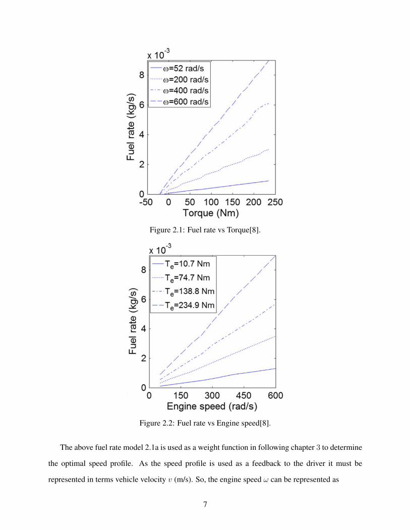
Figure 2.1: Fuel rate vs Torque[8].
Figure 2.2: Fuel rate vs Engine speed[8].
The above fuel rate model 2.1a is used as a weight function in following chapter 3 to determine
the optimal speed profile. As the speed profile is used as a feedback to the driver it must be
represented in terms vehicle velocity v (m/s). So, the engine speed ω can be represented as
7

Figure 2.3: Fuel map[8].
ω =frgr(n) ∗ v
rw(2.1b)
where fr is a final drive ratio, gr(n) is a gear ratio for a given gear number n, and rw is a wheel
radius (m). By substituting Equation 2.1b into fuel rate function 2.1a gives us following equation:
mf =
(β1frgr(n)
rwv + β2
)Te + γ1
frgr(n)
rwv + γ2 (2.1c)
where v is vehicle speed β1,β2,γ1,γ2 are constants.
The constant values are:
β1 = 5.646 × 10⁻⁸
β2 = 4.751 × 10⁻⁷
γ1 = 1.625 × 10⁻⁶
8
γ2 = −5.968 × 10⁻⁵
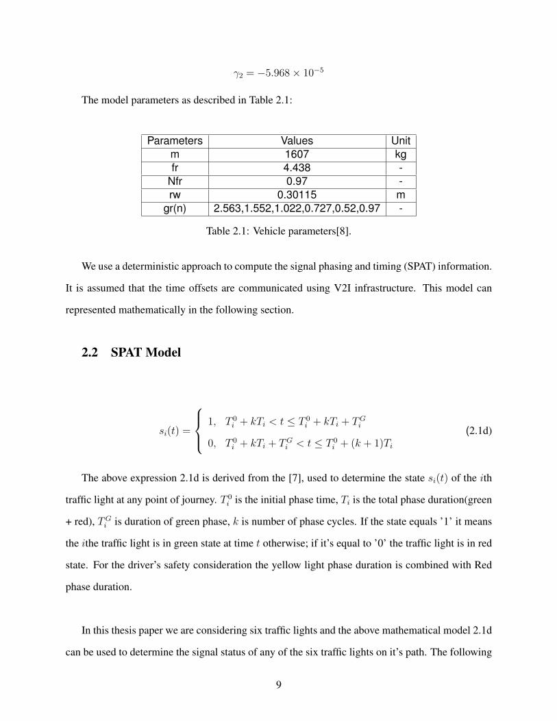
The model parameters as described in Table 2.1:
Parameters Values Unitm 1607 kgfr 4.438 -
Nfr 0.97 -rw 0.30115 m
gr(n) 2.563,1.552,1.022,0.727,0.52,0.97 -
Table 2.1: Vehicle parameters[8].
We use a deterministic approach to compute the signal phasing and timing (SPAT) information.
It is assumed that the time offsets are communicated using V2I infrastructure. This model can
represented mathematically in the following section.
2.2 SPAT Model
si(t) =
1, T 0i + kTi < t ≤ T 0
i + kTi + TGi
0, T 0i + kTi + TG
i < t ≤ T 0i + (k + 1)Ti
(2.1d)
The above expression 2.1d is derived from the [7], used to determine the state si(t) of the ith
traffic light at any point of journey. T 0i is the initial phase time, Ti is the total phase duration(green
+ red), TGi is duration of green phase, k is number of phase cycles. If the state equals ’1’ it means
the ithe traffic light is in green state at time t otherwise; if it’s equal to ’0’ the traffic light is in red
state. For the driver’s safety consideration the yellow light phase duration is combined with Red
phase duration.
In this thesis paper we are considering six traffic lights and the above mathematical model 2.1d
can be used to determine the signal status of any of the six traffic lights on it’s path. The following
9

figures 2.4,2.5, 2.6, 2.7, 2.8,2.9 represents the signal phase changes for six traffic lights over a
period of 400 seconds.
Traffic light 1 signal status:
T 0i = 20 sec
Ti = 15 sec
TGi = 15 sec
Figure 2.4: Signal status for Traffic light 1.
Traffic light 2 signal status:
T 0i = 5 sec
Ti = 8 sec
TGi = 8 sec
Figure 2.5: Signal status for Traffic light 2.
10

Traffic light 3 signal status:
T 0i = 10 sec
Ti = 25 sec
TGi = 25 sec
Figure 2.6: Signal status for Traffic light 3.
Traffic light 4 signal status:
T 0i = 10 sec
Ti = 15 sec
TGi = 15 sec
Figure 2.7: Signal status for Traffic light 4.
11

Traffic light 5 signal status:
T 0i = 20 sec
Ti = 15 sec
TGi = 15 sec
Figure 2.8: Signal status for Traffic light 5.
Traffic light 6 signal status:
T 0i = 10 sec
Ti = 20 sec
TGi = 20 sec
Figure 2.9: Signal status for Traffic light 6.
12

When the vehicle is approaching the 6th traffic light with in 200 seconds the vehicle can have
a very smooth transition at the traffic intersection without stopping as shown in the figure 2.10.
Figure 2.10: Vehicle passing through traffic intersection during Green phase.
13

CHAPTER III
Optimization problem
The optimization problem is to find optimal speed profile using Dijkstra algorithm among all
the available crossing speeds at each traffic intersection. The weighted matrix consists of the fuel
energy consumed in each path.
Figure 3.1: Crossing window algorithm[7].
The following sections describe the algorithm used to create the weighted adjacency matrix
using the feasible crossing windows at each intersection. The crossing window search algorithm
adapted from [7] uses the speed profile calculation based on basic discrete time integration and
14

basic vehicle kinematic equations. Figure 3.1 shows the authors implementation of cross window
search algorithm. The authors algorithms determines all the possible crossing windows at each
intersection but doesn’t generate the adjacency matrix; which can be used as an input for various
optimization algorithms. Here we extend that algorithm further to generate adjacency matrix in
the same code routine, which can be populated with either crossing times or fuel consumption
values as weights to generate the rough estimation of the optimal speed. Further, the authors
used Sequential Quadratic Programming (SQP) method to solve the simplified and the original
optimization problem proposed in paper[7]. In this paper we use Dijkstra algorithm to find the
optimal path. The Dijkstra algorithm is feasible for this approach compared to Floyd-Warshall
algorithm because the weights generated are always positive.
3.1 Cross window search and Adjacency matrix creation Algorithm
The first step is to find all possible crossing windows during the green phase at each traffic
signal intersection. Once the crossing windows are determined we will incorporate matrix indexing
code routine to convert a regular matrix in to adjacency matrix.
Psedo code 1: Cross window search and Adjacency matrix creation Algorithm
1: for i=1 : number of traffic lights
2 : Vmax = min(max speed limit, Vflow)
3: if i=1; Absolute distance=di else equals di − di−1
4 : if i = 1; tfast =Absolute distance
Vmax
else equalst fast =Absolute distance
Vmax
+ tmini−1
5 : find the ith signal status at tfast
6 : while : if status is red increment the search variable till green phase is found
7 : end while
8 : tmaxi,j = next green phase
15

9 : tmini,j = max
(t fast , t
maxi,j − TG
i
)10 : if i = 1; tslow = di−di−1
Vminelse equalstslow = di−di−1
Vmin+ tmax
i−1
11 : while(ttmini,j + Ti < t slow
)do
12 : j = j + 1
13 : tmini,j = tmin
i,j−1 + Ti
14 : tmaxi,j = min
(tmini,j + TG
i , tslow)
15 : end while
16 : concatenate tmini,j and tmax
i,j
17 : Sort the above array in ascending order colounm wise and store in tcombine
18 : Nnzvr2 represents number of non zero values in (i− 1)th row
19 : Nnzvr2 values we determine for each node if the egde is going inwards and outwards
20 : For each iteration adjacency matrix’s for speed(speedadj) and fuel(fuelwtadj)
consumption are populated.
21 : For fuelwtadj matrix negative weights are made zero
22 : Both the adjacency matrix’s are converted in to square matrix
23 : end while
In the above Psedo code 1 steps 1 through 14 minimizes the search space of available cross
windows during green phases by identifying only feasible windows that will allow the driver to
reach the destination without stopping at any traffic intersection by compiling to the speed limits
and traffic flow. For each iteration we first compute the Vmax. Which is the minimum value among
the maximum speed and traffic flow speed. After that we calculate the tfast to check whether the
vehicle can reach the ith traffic intersection before the traffic light turns to red. If the computed
tfast wouldn’t help the vehicle to reach during green crossing time; we will find the next possible
green window and assign that time to tmaxi,j . If the computed ttmin
i,j + Ti < t slow it means that there
are still feasible crossing windows available. These new feasible windows are populated and stored
in tmaxi,j and tmin
i,j .
16
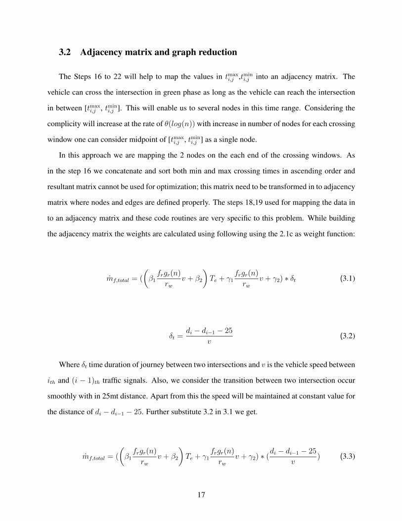
3.2 Adjacency matrix and graph reduction
The Steps 16 to 22 will help to map the values in tmaxi,j ,tmin
i,j into an adjacency matrix. The
vehicle can cross the intersection in green phase as long as the vehicle can reach the intersection
in between [tmaxi,j , tmin
i,j ]. This will enable us to several nodes in this time range. Considering the
complicity will increase at the rate of θ(log(n)) with increase in number of nodes for each crossing
window one can consider midpoint of [tmaxi,j , tmin
i,j ] as a single node.
In this approach we are mapping the 2 nodes on the each end of the crossing windows. As
in the step 16 we concatenate and sort both min and max crossing times in ascending order and
resultant matrix cannot be used for optimization; this matrix need to be transformed in to adjacency
matrix where nodes and edges are defined properly. The steps 18,19 used for mapping the data in
to an adjacency matrix and these code routines are very specific to this problem. While building
the adjacency matrix the weights are calculated using following using the 2.1c as weight function:
mf,total = (
(β1frgr(n)
rwv + β2
)Te + γ1
frgr(n)
rwv + γ2) ∗ δt (3.1)
δt =di − di−1 − 25
v(3.2)
Where δt time duration of journey between two intersections and v is the vehicle speed between
ith and (i − 1)th traffic signals. Also, we consider the transition between two intersection occur
smoothly with in 25mt distance. Apart from this the speed will be maintained at constant value for
the distance of di − di−1 − 25. Further substitute 3.2 in 3.1 we get.
mf,total = (
(β1frgr(n)
rwv + β2
)Te + γ1
frgr(n)
rwv + γ2) ∗ (
di − di−1 − 25
v) (3.3)
17

The transition phase fuel consumption parameters are computed after the optimal speed profile
is determined.
3.3 Optimal path
The wights of adjacency matrix are always positive in this application as the fuel rate is positive
variable and cannot go negative. For non negative weights Dijkstra algorithm is best suitable opti-
mization algorithm. We are using the Dijkstra in this application because of it’s simple approach
and faster computing time considering our real-time use in driving scenarios.
Before apply the the Dijkstra algorithm. We need to transform the adjacency matrix into square
matrix. After the conversion the algorithm can be applied. In this work we are using the Dijkstra
algorithm from matlab toolbox[mlab]. The algorithm provides route with low fuel consumption.
This information is used to create the optimal speed profile. The application of Dijkstra algorithm
and simulation results are further discussed in the following chapter 4.
For example for the following parameters; if we run psedo code 1 with the following parame-
ters:
Vmin = 14 mts/sec
Vspeedlimit = 35 mts/sec
Vflow = [16, 25, 25, 21, 16, 24] mts/sec
di = [800, 1500, 2200, 3000, 3500, 4500] mts
The results for cross windows regions are as given in the for each traffic light:
Traffic light 1:
tmin = 51 sec
tmax = 66 sec
18

Figure 3.2: Crossing window for Traffic light 1. x-axis: time(sec), y-axis:signal status(1 or 0).
Traffic light 2:
tmin = 90 sec
tmax = 98 sec
Figure 3.3: Crossing window for Traffic light 2. x-axis: time(sec), y-axis:signal status(1 or 0).
Traffic light 3:
tmin = 118 sec
tmax = 122 sec
Figure 3.4: Crossing window for Traffic light 3. x-axis: time(sec), y-axis:signal status(1 or 0).
Traffic light 4:
tmin = 170.09 sec
tmax = 185.09 sec
19

Figure 3.5: Crossing window for Traffic light 4. x-axis: time(sec), y-axis:signal status(1 or 0).
Traffic light 5:
tmin = 201.34 sec
tmax = 215.34 sec
Figure 3.6: Crossing window for Traffic light 5. x-axis: time(sec), y-axis:signal status(1 or 0).
Traffic light 6:
tmin = 243.01 sec
tmax = 255.01 sec
Figure 3.7: Crossing window for Traffic light 6. x-axis: time(sec), y-axis:signal status(1 or 0).
20

The tmin represents figure 3.8 the earliest time vehicle cross the traffic intersection without
stopping and tmax represents figure 3.9 the final time the vehicle has to reach the traffic light be-
fore traffic light turn red.
Figure 3.8: tmin crossing point for Traffic light 1.
Figure 3.9: tmax crossing point for Traffic light 1.
21

In order for the vehicle to reach the destination without stopping; The vehicle has to cross the
intersection during the green windows figure 3.10 . By using the optimal path approach the vehicle
not only crosses the green windows but also it can be optimized to find the best fuel economical
path.
Figure 3.10: Vehicle trajectory through green crossing windows.
For the optimization using Dijkstra algorithm each tmax and tmin values for 6 traffic lights are
considered as individual nodes as shown in figure 3.11.
22

Figure 3.11: Node structure for Dijkstra algorithm.
After feeding the tmax and tmin values into Adjacency matrix code routine it will generate the
adjacency matrix figure 3.12.
Figure 3.12: Adjacency Matrix.
The Adjacency matrix is used to find the lowest weighted path by using Dijkstra algorithm.
The results of Dijkstra algorithm are shown in figure 3.13. Where the lowest weighted path in
terms of fuel weight is Node1− > 2− > 4− > 6− > 8− > 11− > 13.
23

Figure 3.13: Directed graph with fuel weights.
24

CHAPTER IV
Integration of ”nonstop” model to distance based long term optimization
The optimization model that generates optimal speed profile as described in the previous chap-
ters can be called as ”Nonstop” model. This model generates an optimal speed profile; When a
vehicle follows the generated speed profile it can drive through traffic signal intersections with out
stopping. Thus saving fuel by minimizing excessive acceleration and idling at traffic signal stops.
In the following sub sections we will look into integrated and standalone simulation results of
”Nonstop” model.
4.1 Distance based Eco driving scheme long term optimization
The paper ”A Distance-Based Two-Stage Ecological Driving System Using an Estimation of
Distribution Algorithm and Model Predictive Control”[2] extends a two-stage ecological driving
system optimized in a distance domain by using an EDA and MPC, which consists of a long-term
optimization stage and a local adaptation stage. The former stage optimizes the speed profile for
an entire trip route without consideration for traffic conditions before departure. The latter stage
utilizes the optimal speed profile given by the former stage as a reference speed and adapts the
reference speed for a short horizon according to actual traffic conditions while driving. In order
to localize the change in the optimal speed profile due to traffic conditions, the optimization was
performed in a distance domain.
The long-term optimization[2] cost function is given below:
Jopt = w1
n−1∑k=0
mf (k)∆tk + w2
n−1∑k=0
(v(k + 1)2 − V target (k + 1)2
)2 (4.1)
25

where mf is fuel rate model,w1,w2 are weight that can be varied based on the driver’s prefer-
ences. v(k+1) and v target (k+1) are the vehicle current speed and target speeds[2]. The long-term
optimization doesn’t consider the SPAT information to schedule the optimal speed.
The ”Nonstop” model proposed in this thesis paper can narrow down the speed profile using
the SPAT information and this data can be fed to the v target (k + 1) for further optimization. As
the proposed model takes less computational time over short horizons it’s favorable for online
implementation and integration as a feature to the existing optimal solutions.
Figure 4.1: Two-Stage Ecological Driving Scheme[2].
Let’s look in detail into distance-based two-stage ecological driving system[2]. Figure 4.1
gives an overview of this approach. The eco driving system is divided into two stages first stage is
long term optimization. In this stage the speed is optimized for the entire horizon by considering
characteristic of drive train and road slopes and speed limits. This optimization is performed
before departure. When the vehicle is on move the local optimization comes into picture. In local
optimization the speed is followed by considering the optimal speed generated in the long term
optimization along with traffic conditions. In areas under heavy traffic conditions the speed is
optimized considering the distance from the preceding vehicle.
In a speed profile defined in a time domain, any deviation from the optimal speed profile due to
traffic conditions changes the entire reference speed after that time, which requires re-optimization
26

for the whole remaining route. By comparison, in a speed profile defined in a distance domain, any
deviation affects only areas under heavy traffic conditions and the reference speeds of other areas
are still effective. That is the reason why this optimization is performed in a distance domain[2].
For optimization of cost function authors used EDA algorithm.
4.2 Simulation and Results
For this simulation the vehicle path trajectory is considered to be straight line and has traffic lights
at different locations ”di” mts. The matrix di consists of distance of 6 traffic lights from the
origin. The ”SPAT” information in sec, phase cycles k and distance data for each 6 traffic lights
are as follows:
T 0i = [20, 5, 10, 10, 20, 10] sec
Ti = [15, 8, 25, 15, 15, 20] sec
TGi = [15, 8, 25, 15, 15, 20] sec
k = 100
di = [1200, 2000, 2900, 3800, 4500, 5000] mts
The maximum speed limit is [16, 25, 25, 21, 16, 24] , Vmin and vehicle flow Vflow are as follows:
Vmin = 1.38 mts/sec
Vflow = [16, 25, 25, 21, 16, 24] mts/sec
The vehicle parameters and fuel model are derived from ”A Distance-Based Two-Stage
Ecological Driving System Using an Estimation of Distribution Algorithm and Model Predictive
Control”[2]. The above mentioned parameters are used to determine the optimal speed profile
using the psedocode1. The standalone and integrated simulations results are discussed in the
following sections.
27
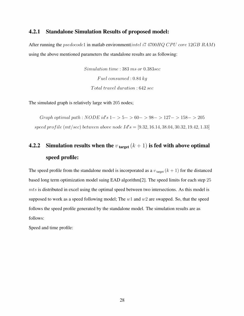
4.2.1 Standalone Simulation Results of proposed model:
After running the psedocode1 in matlab environment(intel i7 4700HQ CPU core 12GB RAM )
using the above mentioned parameters the standalone results are as following:
Simulation time : 383 ms or 0.383sec
Fuel consumed : 0.84 kg
Total travel duration : 642 sec
The simulated graph is relatively large with 205 nodes;
Graph optimal path : NODE id′s 1− > 5− > 60− > 98− > 127− > 158− > 205
speed profile (mt/sec) between above node Id′s = [9.32, 16.14, 38.04, 30.32, 19.42, 1.33]
4.2.2 Simulation results when the v target (k + 1) is fed with above optimal
speed profile:
The speed profile from the standalone model is incorporated as a v target (k + 1) for the distanced
based long term optimization model suing EAD algorithm[2]. The speed limits for each step 25
mts is distributed in excel using the optimal speed between two intersections. As this model is
supposed to work as a speed following model; The w1 and w2 are swapped. So, that the speed
follows the speed profile generated by the standalone model. The simulation results are as
follows:
Speed and time profile:
28

Figure 4.2: speed and time profile.
Torque and brake profile:
Figure 4.3: torque and brake profile.
Simulation time : 41.84 sec
Fuel consumed : 0.36 kg
Total travel duration : 640 sec
29
4.2.3 Case Studies
In this section we will look into results by varying different parameters.
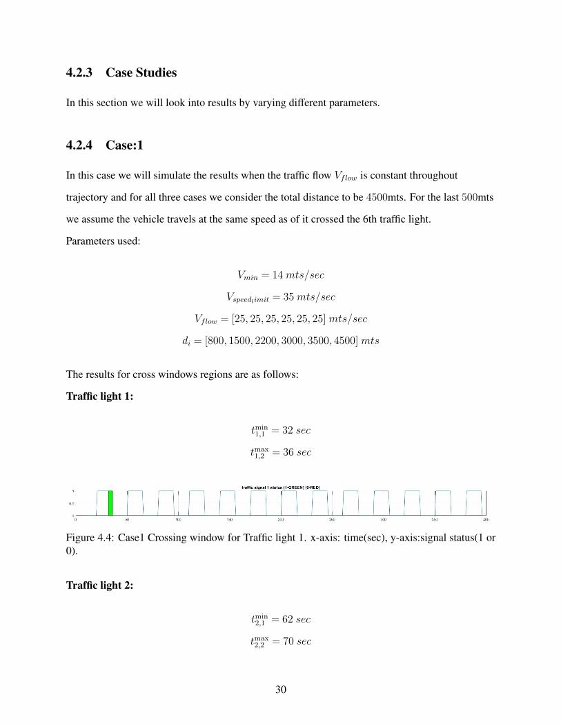
4.2.4 Case:1
In this case we will simulate the results when the traffic flow Vflow is constant throughout
trajectory and for all three cases we consider the total distance to be 4500mts. For the last 500mts
we assume the vehicle travels at the same speed as of it crossed the 6th traffic light.
Parameters used:
Vmin = 14 mts/sec
Vspeedlimit = 35 mts/sec
Vflow = [25, 25, 25, 25, 25, 25] mts/sec
di = [800, 1500, 2200, 3000, 3500, 4500] mts
The results for cross windows regions are as follows:
Traffic light 1:
tmin1,1 = 32 sec
tmax1,2 = 36 sec
Figure 4.4: Case1 Crossing window for Traffic light 1. x-axis: time(sec), y-axis:signal status(1 or0).
Traffic light 2:
tmin2,1 = 62 sec
tmax2,2 = 70 sec
30

Figure 4.5: Case1 Crossing window for Traffic light 2. x-axis: time(sec), y-axis:signal status(1 or0).
Traffic light 3:
tmin3,1 = 97 sec
tmax3,2 = 122 sec
Figure 4.6: Case1 Crossing window for Traffic light 3. x-axis: time(sec), y-axis:signal status(1 or0).
Traffic light 4:
tmin4,1 = 131 sec
tmax4,2 = 146 sec
tmin4,3 = 171 sec
tmax4,4 = 179.14 sec
Figure 4.7: Case1 Crossing window for Traffic light 4. x-axis: time(sec), y-axis:signal status(1 or0).
Traffic light 5:
tmin5,1 = 151 sec
tmax5,2 = 156 sec
tmin5,3 = 181 sec
tmax5,4 = 181.71 sec
31

Figure 4.8: Case1 Crossing window for Traffic light 5. x-axis: time(sec), y-axis:signal status(1 or0).
Traffic light 6:
tmin6,1 = 191 sec
tmax6,2 = 211 sec
Figure 4.9: Case1 Crossing window for Traffic light 6. x-axis: time(sec), y-axis:signal status(1 or0).
In order for the vehicle to reach the destination without stopping; The vehicle has to cross the
intersection during the green windows figure 4.10 . By using the optimal path approach the
vehicle not only crosses the green windows but also it can be optimized to find the best fuel
economical path.
Figure 4.10: Case1 Vehicle trajectory through green crossing windows.
32

For the optimization using Dijkstra algorithm each tmax and tmin values for 6 traffic lights are
considered as individual nodes as shown in figure 4.11.
Figure 4.11: Case1 Node structure for Dijkstra algorithm.
After feeding the tmax and tmin values into Adjacency matrix code routine it will generate the
adjacency matrix figure 4.13
Figure 4.12: Case1 Adjacency Matrix.
The Adjacency matrix is used to find the lowest weighted path by using Dijkstra algorithm. The
results of Dijkstra algorithm are shown in figure 4.13 . Where the lowest weighted path in terms
33

of fuel weight is Node1 − 2 − 5 − 6 − 9 − 13 − 17.
Figure 4.13: Case1 Directed graph with fuel weights.
34

After running the psedocode1 in matlab environment(intel i7 4700HQ CPU core 12GB RAM )
using the above mentioned parameters the standalone results are as following:
Simulation time : 71 ms or 0.071sec
Fuel consumed : 0.38 kg
Total travel duration : 217.95 sec
The simulated graph has 17 nodes;
Graph optimal path : NODE id′s 1− > 2− > 5− > 6− > 9− > 13− > 17
speed profile (mt/sec) between above node Id′s = [24.21, 17.76, 25, 15.81, 47.5, 17.72]
The speed profile from the standalone model is incorporated as a v target (k + 1) for the distanced
based long term optimization model suing EAD algorithm[2]. The speed limits for each step 25
mts is distributed in excel using the optimal speed between two intersections. As this model is
supposed to work as a speed following model; The w1 and w2 are swapped. So, that the speed
follows the speed profile generated by the standalone model. The simulation results are as
follows:
Speed and time profile:
Figure 4.14: Case1 speed and time profile.
Torque and brake profile:
35

Figure 4.15: Case1 torque and brake profile.
Simulation time : 30.73 sec
Fuel consumed : 0.35 kg
Total travel duration : 256.53 seconds
In the Case1 we observed that with the Vflow of traffic being constant the fuel consumed is less,
travel time is less, simulation time is improved.
case2
4.2.5 Case:2
In this case we will simulate the results when the traffic flow Vflow is closer to Vmaxlimit
throughout trajectory.
Parameters used:
Vmin = 14 mts/sec
Vspeedlimit = 35 mts/sec
Vflow = [30, 30, 30, 30, 30, 30] mts/sec
Vmaxlimit = [35, 35, 35, 35, 35, 35] mts/sec
di = [800, 1500, 2200, 3000, 3500, 4500] mts
The results for cross windows regions are as follows:
36

Traffic light 1:
tmin1,1 = 26.66 sec
tmax1,2 = 35.66 sec
tmin1,3 = 56.66 sec
tmax1,4 = 57.14 sec
Figure 4.16: Case2 Crossing window for Traffic light 1. x-axis: time(sec), y-axis:signal status(1or 0).
Traffic light 2:
tmin2,1 = 62 sec
tmax2,2 = 70 sec
Figure 4.17: Case2 Crossing window for Traffic light 2. x-axis: time(sec), y-axis:signal status(1or 0).
Traffic light 3:
tmin3,1 = 96.33 sec
tmax3,2 = 121.33 sec
Traffic light 4:
37
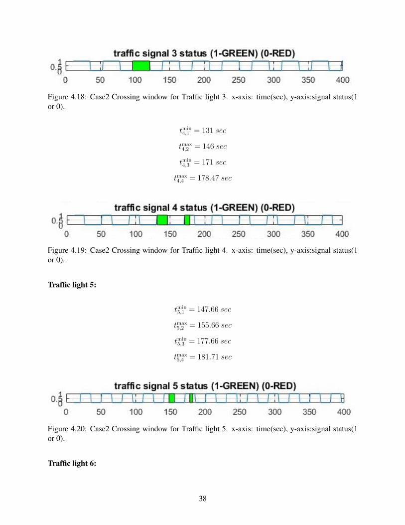
Figure 4.18: Case2 Crossing window for Traffic light 3. x-axis: time(sec), y-axis:signal status(1or 0).
tmin4,1 = 131 sec
tmax4,2 = 146 sec
tmin4,3 = 171 sec
tmax4,4 = 178.47 sec
Figure 4.19: Case2 Crossing window for Traffic light 4. x-axis: time(sec), y-axis:signal status(1or 0).
Traffic light 5:
tmin5,1 = 147.66 sec
tmax5,2 = 155.66 sec
tmin5,3 = 177.66 sec
tmax5,4 = 181.71 sec
Figure 4.20: Case2 Crossing window for Traffic light 5. x-axis: time(sec), y-axis:signal status(1or 0).
Traffic light 6:
38

tmin6,1 = 191 sec
tmax6,2 = 211 sec
Figure 4.21: Case2 Crossing window for Traffic light 6. x-axis: time(sec), y-axis:signal status(1or 0).
In order for the vehicle to reach the destination without stopping; The vehicle has to cross the
intersection during the green windows figure 4.22 . By using the optimal path approach the
vehicle not only crosses the green windows but also it can be optimized to find the best fuel
economical path.
Figure 4.22: Case2 Vehicle trajectory through green crossing windows.
For the optimization using Dijkstra algorithm each tmax and tmin values for 6 traffic lights are
considered as individual nodes as shown in figure 3.11.
39

Figure 4.23: Case2 Node structure for Dijkstra algorithm.
After feeding the tmax and tmin values into Adjacency matrix code routine it will generate the
adjacency matrix figure 4.13
Figure 4.24: Case2 Adjacency Matrix.
The Adjacency matrix is used to find the lowest weighted path by using Dijkstra algorithm. The
results of Dijkstra algorithm are shown in figure 4.25 . Where the lowest weighted path in terms
of fuel weight is Node1 − 2 − 7 − 8 − 11 − 16 − 19.
Simulation time : 59 ms or 0.0599sec
40
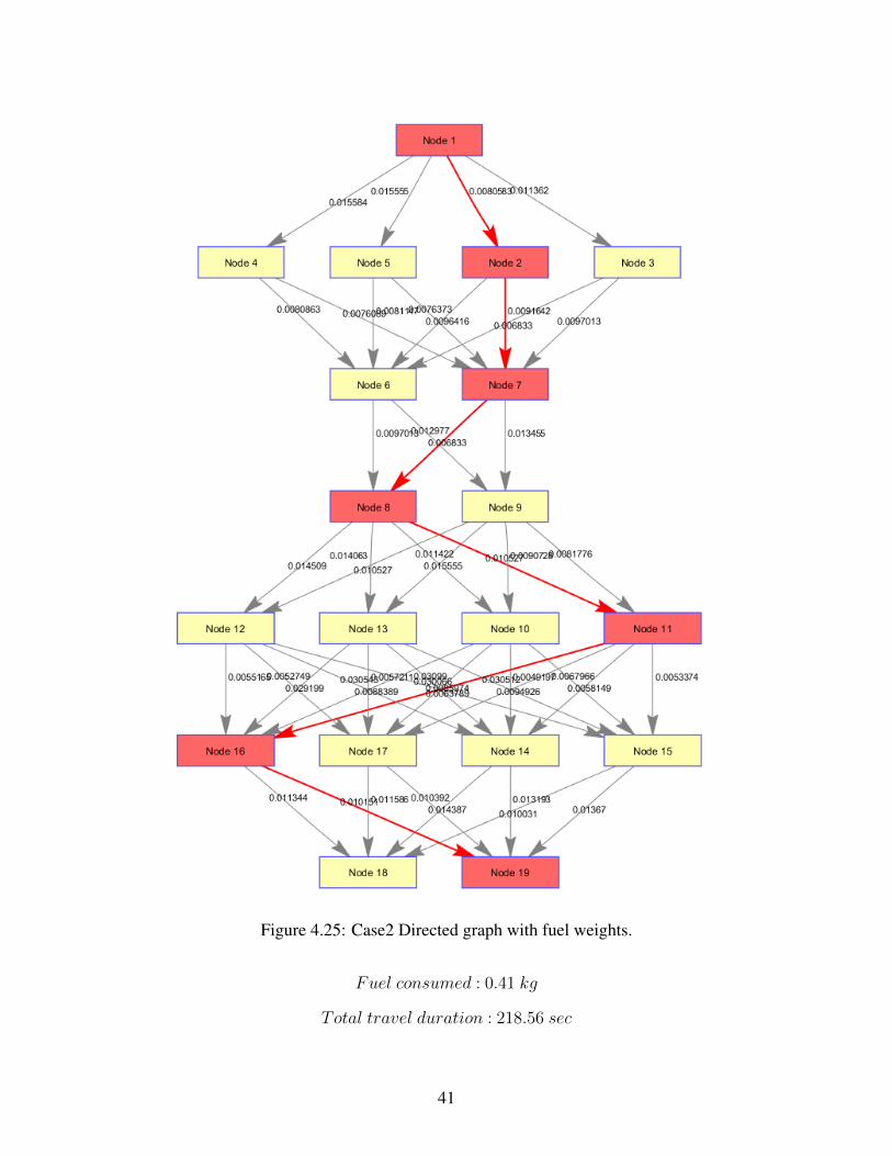
Figure 4.25: Case2 Directed graph with fuel weights.
Fuel consumed : 0.41 kg
Total travel duration : 218.56 sec
41

The simulated graph is of 19 nodes;
Graph optimal path : NODE id′s 1− > 2− > 7− > 8− > 11− > 16− > 19
speed profile (mt/sec) between above node Id′s = [29.06, 15.57, 25.63, 15.60, 15, 29.25]
The speed profile from the standalone model is incorporated as a v target (k + 1) for the distanced
based long term optimization model suing EAD algorithm[2]. The speed limits for each step 25
mts is distributed in excel using the optimal speed between two intersections. As this model is
supposed to work as a speed following model; The w1 and w2 are swapped. So, that the speed
follows the speed profile generated by the standalone model. The simulation results figures are as
follows:
Speed and time profile:
Figure 4.26: Case2 speed and time profile.
Torque and brake profile:
Simulation time : 23.31 sec
42

Figure 4.27: Case2 torque and brake profile.
Fuel consumed : 0.36 kg
Total travel duration : 262.20 seconds
In the Case2 we observed that with the Vflow of traffic being constant the fuel consumed is less,
travel time is less, simulation time is improved.
4.2.6 Case:3
In this case we will simulate the results when the traffic flow TGi is constant throughout trajectory
while considering the case2 conditions for traffic conditions.
Parameters used:
TGi = [10, 10, 10, 10, 10, 10] sec
Vmin = 14 mts/sec
Vspeedlimit = 35 mts/sec
Vflow = [30, 30, 30, 30, 30, 30] mts/sec
di = [800, 1500, 2200, 3000, 3500, 4500] mts
43

The results for cross windows regions are as follows:
Traffic light 1:
tmin1,1 = 26.66 sec
tmax1,2 = 35.66 sec
tmin1,3 = 51.66 sec
tmax1,4 = 57.14 sec
Figure 4.28: Case3 Crossing window for Traffic light 1. x-axis: time(sec), y-axis:signal status(1or 0).
Traffic light 2:
tmin2,1 = 60 sec
tmax2,2 = 70 sec
Figure 4.29: Case3 Crossing window for Traffic light 2. x-axis: time(sec), y-axis:signal status(1or 0).
Traffic light 3:
tmin3,1 = 111.33 sec
tmax3,2 = 121.33 sec
Traffic light 4:
44

Figure 4.30: Case3 Crossing window for Traffic light 3. x-axis: time(sec), y-axis:signal status(1or 0).
tmin4,1 = 138 sec
tmax4,2 = 146 sec
tmin4,3 = 173 sec
tmax4,4 = 178.47 sec
Figure 4.31: Case3 Crossing window for Traffic light 4. x-axis: time(sec), y-axis:signal status(1or 0).
Traffic light 5:
tmin5,1 = 154.66 sec
tmax5,2 = 155.66 sec
tmin5,3 = 179.66 sec
tmax5,4 = 181.71 sec
Figure 4.32: Case3 Crossing window for Traffic light 5. x-axis: time(sec), y-axis:signal status(1or 0).
Traffic light 6:
45

tmin6,1 = 201 sec
tmax6,2 = 211 sec
Figure 4.33: Case3 Crossing window for Traffic light 6. x-axis: time(sec), y-axis:signal status(1or 0).
In order for the vehicle to reach the destination without stopping; The vehicle has to cross the
intersection during the green windows figure 4.34 . By using the optimal path approach the
vehicle not only crosses the green windows but also it can be optimized to find the best fuel
economical path.
Figure 4.34: Case3 Vehicle trajectory through green crossing windows.
For the optimization using Dijkstra algorithm each tmax and tmin values for 6 traffic lights are
considered as individual nodes as shown in figure 4.35.
46

Figure 4.35: Case3 Node structure for Dijkstra algorithm.
After feeding the tmax and tmin values into Adjacency matrix code routine it will generate the
adjacency matrix figure 4.36
Figure 4.36: Case3 Adjacency Matrix.
The Adjacency matrix is used to find the lowest weighted path by using Dijkstra algorithm. The
results of Dijkstra algorithm are shown in figure 4.37 . Where the lowest weighted path in terms
of fuel weight is Node1 − 2 − 7 − 8 − 10 − 15 − 19.
After running the psedocode1 in matlab environment(intel i7 4700HQ CPU core 12GB RAM )
using the above mentioned parameters the standalone results are as following:
47
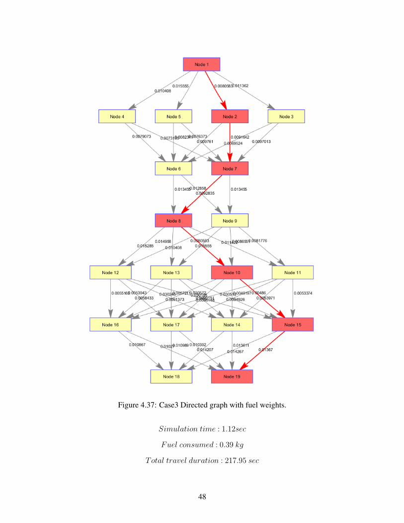
Figure 4.37: Case3 Directed graph with fuel weights.
Simulation time : 1.12sec
Fuel consumed : 0.39 kg
Total travel duration : 217.95 sec
48

The simulated graph has 19 nodes;
Graph optimal path : NODE id′s 1− > 2− > 7− > 8− > 10− > 15− > 19
speed profile (mt/sec) between above node Id′s = [29.06, 15.57, 16.33, 29.06, 26.88, 17.62]
The speed profile from the standalone model is incorporated as a v target (k + 1) for the distanced
based long term optimization model suing EAD algorithm[2]. The speed limits for each step 25
mts is distributed in excel using the optimal speed between two intersections. As this model is
supposed to work as a speed following model; The w1 and w2 are swapped. So, that the speed
follows the speed profile generated by the standalone model. The simulation results are as
follows:
Speed and time profile:
Figure 4.38: Case3 speed and time profile.
Torque and brake profile:
Simulation time : 25.37 sec
Fuel consumed : 0.35 kg
Total travel duration : 243.02 seconds
49

Figure 4.39: Case3 torque and brake profile.
In the Case3 we observed that with the TGi of traffic being constant the fuel consumed is less,
travel time is less, simulation time is improved compared with case2. As the TGi is constant it
improves the predictability of traffic environment.
50

BIBLIOGRAPHY
[1] European Commission Climate Action, “What is the EU doing about climate change?”,https://www.eea.europa.eu/data-and-maps/indicators/greenhouse-gas-emission-trends-6/assessment-1.
[2] H. Lim, C. C. Mi and W. Su, ”A Distance-Based Two-Stage Ecological Driving System Us-ing an Estimation of Distribution Algorithm and Model Predictive Control,” in IEEE Transactionson Vehicular Technology, vol. 66, no. 8, pp. 6663-6675, Aug. 2017.
[3] S. Mandava, K. Boriboonsomsin, M. Barth, “Arterial velocity planning based on trafficsignal information under light traffic conditions”, Proc. 12th International IEEE Conference onIntelligent Transportation Systems ITSC ’09, 2009.
[4] Hunt PB, Robertson DI, Bretherton RD, Winton RI. SCOOT - A Traffic Responsive Methodof Co-Ordinating Signals. Technical Report, TRRL Laboratory Report 1014 1981.
[5] Diakaki C. Integrated Control of Traffic Flow in Corridor Networks. PhD Thesis, TechnicalUniversity of Crete 1999.
[6] Urban traffic control systems; www.its.leeds.ac.uk.
[7] V. A. Butakov and P. Ioannou, ”Personalized Driver Assistance for Signalized IntersectionsUsing V2I Communication,” in IEEE Transactions on Intelligent Transportation Systems, vol. 17,no. 7, pp. 1910-1919, July 2016.
[8] H. Lim, W. Su and C. C. Mi, ”Distance-Based Ecological Driving Scheme Using a Two-Stage Hierarchy for Long-Term Optimization and Short-Term Adaptation,” in IEEE Transactionson Vehicular Technology, vol. 66, no. 3, pp. 1940-1949, March 2017.
[9]https://pxhere.com/en/photo/131869.
51