European Journal of Operational Research 198 (2009) 610–617

Contents lists available at ScienceDirect

European Journal of Operational Research

journal homepage: www.elsevier .com/locate /e jor

Decision Support

An integrated operation module for individual risk management

Hsiao-Fan Wang *, Fei-Chen HsuDepartment of Industrial Engineering and Engineering Management, National Tsing Hua University, No. 101, Section 2 Kuang Fu Road, Hsinchu 30013, Taiwan

a r t i c l e i n f o a b s t r a c t

Article history:Received 29 July 2005Accepted 26 September 2008Available online 10 October 2008

Keywords:IRMPreference structureCumulative prospect theoryRisk analysisRisk response

0377-2217/$ - see front matter � 2008 Elsevier B.V. Adoi:10.1016/j.ejor.2008.09.039

* Corresponding author. Tel.: +886 3 5742654; fax:E-mail addresses: hfwang@ie.nthu.edu.tw (H.-F. W

edu.tw (F.-C. Hsu).URL: http://softlab.ie.nthu.edu.tw (H.-F. Wang).

In this study, we used the cumulative prospect theory to propose the individual risk management process(IRM) which includes risk analysis and risk response stages. According to an individual’s preferentialstructure, the process has been developed into an operational module which includes two sub-modules.From this, the individual’s risk level for the confronted risk can be identified from the risk analysis, whilethe response strategies can be assessed at the risk response stage. Therefore, optimal response strategiescan be recommended based on individual risk tolerance levels.

The applicability of the proposed module is evaluated using an A–C court case. The results show thatthe proposed method can provide more useful and pertinent information than the traditional method ofdecision tree by using the expected monetary value (EMV).

� 2008 Elsevier B.V. All rights reserved.

1. Introduction

Risk management has been widely applied in various fields suchas economics, insurance, industries, and so on. While the word‘‘risk” means that uncertainty can be expressed through probabil-ity, risk management is a structured process for the managementof uncertainty through risk assessment.

Most studies on risk management have focused on the causesand effects of a risk event that occurs in an enterprise or an orga-nization (e.g. Alexander andSheedy, 2004; Borodzicz, 2005). Whilethis is important, follow-up considerations for assessing risks andresponse for an individual of an organization not only can providevaluable information in the face of risks but also effectively resultin impact reduction. However, different individuals take the samerisk event with different degrees of impacts (Ward, 2007). As a con-sequence, the adopted actions will be different from individual toindividual. In addition, studies from individuals’ viewpoints arerarely found in the literature despite their significance, in particu-lar, for an increasingly complex environment especially if an effec-tive strategy were to be proposed for an individual.

Thus, in this study, we intend to base on an individual’s charac-teristics to propose an individual risk management process we callIRM in brief, which includes two parts of risk analysis and risk re-sponse. The risk analysis procedure is to identify the degree of riskwith respect to the individual’s tolerance level, while the risk re-sponse process is to assess the considered response strategy in or-der to provide appropriate action. To ensure the applicability and

ll rights reserved.

+886 3 5722685.ang), u880806@alumni.nthu.

implementation of the process, the quantification and measuresof each stage are investigated and developed into an operation sys-tem including two modules of risk analysis and risk response. Theresult will be evaluated and compared using an illustrative case.

To demonstrate the proposed system, this article is organized asfollows. In Section 2, concepts of risk management and relatedtheoretical backgrounds are introduced. Two operational moduleswhich include a risk classification model with risk magnitude esti-mation for risk analysis, and a decision model for response strategydevelopment are proposed in Section 3 with a summary of theoverall system. An A–C court case will be demonstrated and evalu-ated in Section 4. Finally, the conclusions will be drawn in Section 5.

2. Basic concepts

The study and implementation of risk management have a longhistory (e.g. Fishburn, 1982; Crockford, 1986; Tummala and Leung,1996; Tummala and Burchett, 1999). The risk management process(RMP) provides a systematic structure to assess the consequencesand likelihood of occurrence associated with a given risk event.Risk analysis and risk response are two major parts of RMP(Tummala and Burchett, 1999). At the risk analysis stage, identifi-cation of the risk sources and threats is the main task, while at therisk response stage, evaluation and development of the riskresponse strategies to avoid or control the identified risks are themain goals.

Although risk management procedures have been developedextensively, the lack of consideration of complete factors has beenan issue. Most existing studies have focused on objective evalua-tion and have largely ignored subjective factors which can help dif-ferentiate the different impacts of risk events for different

H.-F. Wang, F.-C. Hsu / European Journal of Operational Research 198 (2009) 610–617 611

individuals and thus allow the adopted actions to be more effec-tive. To address this gap, in this study, we shall introduce the indi-vidual’s subjective values into the process of risk management.

While personal judgments about uncertainty and values areimportant inputs for making any decision, defining an individual’svalue function becomes a preliminary step towards risk analysis.

The concept of utility was proposed by Bernoulli and Cramer inthe 18th century (Bleichrodt and Pinto, 2000; Levy, 2006). They sug-gested that risky monetary options should be evaluated not by theirexpected return but rather by the expectations of the utilities oftheir return. The utility of a gain or loss is measured by the degreeof pleasure (rejoicing) or pain (regret) that the amount gained or lostgenerates (Piney, 2003). The expected utility theory under risk wasproposed by Von Neumann and Morgenstern (2004), and was basedon the strict logic of a human being’s behavioral assumptions. This isthe guiding principle of decision making under risk conditions.

According to the risk attitudes of being risk averse, risk neutral,and risk seeking, one may obtain the parameter of a functionthrough lottery (Goicoechea et al., 1982; Clemen and Reilly,2001). Individuals who are afraid of risk or are sensitive to riskare considered risk averse. Their typical utility curve is upwardand concave. A convex utility curve indicates a risk seeker; thiskind of individual is eager to engage in a challenging task. Finally,the utility function of a risk neutral person is a straight line. Thecharacteristics of being risk neutral are lack of concern about riskand the ability to ignore the risk alternatives confronted. ExpectedMonetary Values (EMV) as conventionally used for risk analysis arebased on risk neutral assumptions (Clemen and Reilly, 2001).

However, in 1979, Kahneman and Tversky discovered that thedecision preferences of human beings violate the axioms of the ex-pected utility theory and thus proposed the prospect theory (PT)(Kahneman and Tversky, 1979). Then the cumulative prospect the-ory (CPT) that incorporated the descriptive advantages of the origi-nal PT and the theoretical advantages of the rank-dependent utility(Chateauneuf and Wakker, 1999) was developed through manyresearchers’ effort (e.g. Tversky and Kahneman, 1992; Fennemaand Wakker, 1997; Neilson and Stowe, 2002).

Instead of using a probability distribution in PT, CPT uses cumu-lative probability to measure the effect on likelihood of occurrence.Therefore, suppose a gamble is composed of n monetary outcomes,x1 6 � � � 6 xk 6 0 6 xkþ1 6 � � � 6 xn which occur with probabilitiesp1; . . . ; pn, respectively. Then the CPT value of the prospectðx1; p1; � � � ; xn; pnÞ can be given by the following formula (Neilsonand Stowe, 2002):

Vðx;pÞ ¼ V�ðx;pÞ þ Vþðx; pÞ ¼Xk

i¼1

p�vðxiÞ þXn

i¼kþ1

pþvðxiÞ ð1Þ

where

p�1 ¼ w�ðp1Þ; p�i ¼ w�Xi

j¼1

pj

!�w�

Xi�1

j¼1

pj

!2 6 i 6 k

pþn ¼ wþðpnÞ; pþi ¼ wþXn

j¼i

pj

!�wþ

Xn

j¼iþ1

pj

!kþ 1 6 i 6 n� 1

The expression Vþ measures the contribution of gains, while V�

measures the contribution of losses by the respective weighted va-lue function v. Therefore, based on this concept, an individual’s risklevel can be assessed by his/her perceived gain and loss of outcomesas expressed by his/her weighted value function, which paves theway to analyze an individual’s risk tolerance

With regard to the risk response stage, studies emphasized themethod of developing the strategies, giving no consideration to theimpact of the response action. To effectively develop a cost-effec-tive strategy, we shall propose a method to first apply an individ-

ual’s risk tolerance to classify the personal tolerance zones asdefined by Piney (2003). Then according to the properties of eachtolerance zone, the respective strategy can be developed.

Regarding Piney (2003)’s tolerance zones of the dead zone, therational zone, the sensitivity zone, and the saturation zone, withrespect to the magnitude of influence, the idea was to link riskmanagement and cognitive psychology to identify four personalrisk zones in consideration of the gains and losses of the outcomes.Since the conceptual description of these zones causes difficulty inimplementation, we shall therefore propose a classification modelto operate it. Then by analyzing the risk magnitude of each zone, adecision model for developing a respective response strategy willbe provided.

Based on these basic concepts, in the following section, we shalldevelop an operation system for individual risk management.

3. The proposed operation system for the Individual RiskManagement Process (IRM)

Based on the basic concepts described above, we shall developin this section each module in details. Section 3.1 illustrates therisk analysis module, while Section 3.2 develops the risk responsemodule. Finally, we summarize the proposed IRM in Section 3.3.

3.1. Risk analysis module

In this section, an operational model for assessing the risk levelsbased on individual preferences is introduced. A measure of risk le-vel is defined, and the risk zones are classified accordingly.

3.1.1. Individuals’ risk levels and risk zonesBased on the concept of utility, let us first define an individual’s

value functions as follows:

vðxÞ ¼ 1� e�x=R for risk aversione�x=R � 1 for risk seeking

(ð2Þ

where x is the outcome of a risk event and R is risk tolerance: whenR > 0, it is risk aversion; when R < 0, it is risk seeking.

The value of R can be derived from a reference game, typicallyusing the lowest and highest monetary values as references forassessing the points in between. Whenever individuals accept acertainty equivalent which is lesser (greater) than the expected va-lue of the game, they are risk averters (risk seekers), and function vis concave downward (upward) with R>0 (R<0); otherwise, func-tion v is a straight line for risk neutrals (Goicoechea et al., 1982;Clemen and Reilly, 2001)

Then based on the cumulative prospect theory (Neilson andStowe, 2002), an individual’s preference towards a risk event canbe described by a value function, which is weighted by probabilityas follows:

Vðx;pÞ ¼ V�ðx;pÞ þ Vþðx;pÞ ¼Xk

i¼1

p�vðxiÞ þXn

i¼kþ1

pþvðxiÞ

¼Xk

i¼1

e� � ln

Pi

j¼1

pj

� �c

� e� � ln

Pi�1

j¼1

pj

� �c2664

3775vðxiÞ

þXn

i¼kþ1

e� � ln

Pn

j¼i

pj

� �c

� e� � ln

Pn

j¼iþ1

pj

� �c2664

3775vðxiÞ ð3Þ

where ðxi;piÞ is the outcome xi of risk event and its correspondingprobabilities, pi; n is a risk event composed of n monetary out-comes; k is the number of negative outcomes; V is the CPT value

612 H.-F. Wang, F.-C. Hsu / European Journal of Operational Research 198 (2009) 610–617

of the prospect ðx1;p1; � � � ; xn;pnÞ; v is a value function; c is a controlparameter of the curvature of probability weighting function and pis the probability weighting function with

wðpÞ ¼ e�ð� ln pÞc ðPrelec; 1998Þ ð4Þ

According to the idea of Piney (2003), the slope is the main crite-rion dividing utility functions into four risk zones. Therefore, by dif-ferentiating the function V, we define Risk Level by the slope of V as

V 0ðx;pÞ ¼Xk

i¼1

cPij¼1pj

!� ln

Xi

j¼1

pj

!c�1

e� � ln

Pi

j¼1

pj

� �c0BB@

1CCA

2664

� cPi�1j¼1pj

!� ln

Xi�1

j¼1

pj

!e� � ln

Pi�1

j¼1

pj

� �c0BB@

1CCA3775v 0ðxiÞ

þXn

i¼kþ1

cPnj¼ipj

!� ln

Xn

j¼i

pj

!c�1

e� � ln

Pn

j¼i

pj

� �c0BB@

1CCA

2664

� cPnj¼iþ1pj

!� ln

Xn

j¼iþ1

pj

!c�1

e� � ln

Pn

j¼iþ1

pj

� �c0BB@

1CCA3775v 0ðxiÞ

ð5Þ

where

v 0ðxiÞ ¼e�xi=R

R for risk aversion

� e�xi=R

R for risk seeking:

(

Given the number of clusters (four clusters) and the attribute(slope), we used the c-means clustering method (Kaufman andRousseeuw, 1990) to classify the weighted value function into fourrisk zones based on the slope of V.

To illustrate this procedure, we used MATLAB to execute theclustering procedure. Let us consider the initial data as follows:

1. Each risk event is composed of three possible outcomes, i.e.n ¼ 3.

2. Each clustering process includes 1000 risk events.3. Number of iteration = 30.4. Number of clusters = 4.

Then, by giving the risk tolerance, R with the incremental valueof 100 each time from 500 to 10,000 for R 6 1000 and 1000 for

Table 1Slope interval of each risk zone for negative

Pipixi .

NegativeP

ipixi Zone 1 Zone 2

Risk tolerance Lower bound Upper bound Lower bound Upper b

10000 1.1797E�04 2.0656E�04 2.0656E�04 2.5649E9000 1.1768E�04 2.3938E�04 2.3938E�04 3.0302E8000 1.4545E�04 2.8735E�04 2.8735E�04 3.7055E7000 1.5797E�04 3.4672E�04 3.4672E�04 4.6047E6000 1.9489E�04 4.6661E�04 4.6661E�04 6.4077E5000 2.3074E�04 6.4626E�04 6.4626E�04 9.4183E4000 2.9714E�04 1.0887E�03 1.0887E�03 1.7279E3000 4.2698E�04 2.4795E�03 2.4795E�03 4.4295E2000 7.0315E�04 1.2828E�02 1.2828E�02 2.7267E1000 1.7418E�03 2.3761E+00 2.3761E+00 6.4820E

900 1.4667E�03 7.3436E+00 7.3436E+00 2.0871E800 2.4846E�03 3.3044E+01 3.3044E+01 9.4394E700 2.7630E�03 2.1778E+02 2.1778E+02 6.3563E600 3.5148E�03 2.6080E+03 2.6080E+03 7.8762E500 5.4926E�03 8.1553E+04 8.1553E+04 2.5353E

R > 1000, and c ¼ 0:74 as suggested by Wu and Gonzalez(1996) for model (5), the results are shown in Tables 1 and 2 fornegative

Pipixi and positive

Pipixi, respectively.

From Tables 1 and 2, individuals’ risk zones with respect to theirtolerance levels can be well defined by their boundaries. After theperson’s risk zones have been determined, the risk analysis of a riskevent can be done by first obtaining the slope interval of each riskzone according to his/her risk tolerance. Then the risk level for therisk event can be calculated, and under which risk zone the riskevent falls can be determined. Thus, the severity of the confrontedrisk event can be revealed. Based on this result, a suitable responseaction can then be recommended.

To apply the results from risk analysis, we used regression anal-ysis to determine the relations between risk tolerance and the pos-sibility of each risk zone as well as the slope interval of each riskzone.

3.1.2. Regression model for the possibility of each risk zoneAccording to the clustering result, a polynomial regression

model was applied to fit the number of risk events falling into eachrisk zone of which the regressor variable R represents risk toler-ance, and the response y represents the number of each risk zone.Therefore, we can obtain four regression models for each risk zone,as shown below:

yZone i ¼ ðb0 þ b1Rþ b2R2 þ � � � þ bnRn þ eÞi; i ¼ 1 � 4: ð6Þ

Then the possibility of each risk zone can be obtained by its per-centage as

Possibility of Zone i¼ yZone i

yZone 1 þ yZone 2 þ yZone 3 þ yZone 4 ; i¼ 1� 4:

ð7Þ

According to these functions, we can understand the possibility forthe risk zone each person falls into. This helps us comprehend thedistribution of risk events for a specific individual, and the tolerancefor risk in general.

For example, with the same data above, we obtained the regres-sion models for the numbers in each risk zone as listed in Table 3.

Therefore, the possibility of each risk zone is obtained as shownin Table 4. Then once the risk tolerance is known, the possibilitythat the individual might fall in this risk zone can be identifiedwith respect to the outcomes of the risk event faced.

3.1.3. Analysis of the slope interval of each risk zoneTo facilitate the prediction and applications, the possible slope

interval of each risk zone with respect to R is investigated in this

Zone 3 Zone 4

ound Lower bound Upper bound Lower bound Upper bound

�04 2.5649E�04 3.2141E�04 3.2141E�04 5.0666E�04�04 3.0302E�04 3.8154E�04 3.8154E�04 6.1740E�04�04 3.7055E�04 4.7522E�04 4.7522E�04 7.8622E�04�04 4.6047E�04 6.0896E�04 6.0896E�04 1.0796E�03�04 6.4077E�04 8.5671E�04 8.5671E�04 1.5057E�03�04 9.4183E�04 1.2968E�03 1.2968E�03 2.5717E�03�03 1.7279E�03 2.4576E�03 2.4576E�03 5.1738E�03�03 4.4295E�03 6.5526E�03 6.5526E�03 1.4759E�02�02 2.7267E�02 4.3846E�02 4.3846E�02 1.0605E�01+00 6.4820E+00 1.1565E+01 1.1565E+01 2.6799E+01+01 2.0871E+01 3.8122E+01 3.8122E+01 8.4790E+01+01 9.4394E+01 1.7042E+02 1.7042E+02 3.4926E+02+02 6.3563E+02 1.1772E+03 1.1772E+03 2.6626E+03+03 7.8762E+03 1.4537E+04 1.4537E+04 3.1900E+04+05 2.5353E+05 4.7929E+05 4.7929E+05 1.0192E+06

Table 2Slope interval of each risk zone for positive

Pipixi .

PositiveP

ipixi Zone 1 Zone 2 Zone 3 Zone 4

Risk tolerance Upper bound Lower bound Upper bound Lower bound Upper bound Lower bound Upper bound Lower bound

10000 3.5300E�04 2.2337E�04 2.2337E�04 1.6941E�04 1.6941E�04 1.2331E�04 1.2331E�04 5.9293E�059000 4.1491E�04 2.5593E�04 2.5593E�04 1.9069E�04 1.9069E�04 1.3500E�04 1.3500E�04 5.6600E�058000 5.2176E�04 3.1013E�04 3.1013E�04 2.2398E�04 2.2398E�04 1.5198E�04 1.5198E�04 5.9172E�057000 6.5062E�04 3.9951E�04 3.9951E�04 2.7512E�04 2.7512E�04 1.7462E�04 1.7462E�04 5.1763E�056000 9.4892E�04 5.3723E�04 5.3723E�04 3.5280E�04 3.5280E�04 2.0874E�04 2.0874E�04 5.3678E�055000 1.4737E�03 8.3337E�04 8.3337E�04 5.1617E�04 5.1617E�04 2.7734E�04 2.7734E�04 4.5127E�054000 2.8939E�03 1.6415E�03 1.6415E�03 9.5943E�04 9.5943E�04 4.5301E�04 4.5301E�04 3.5789E�053000 8.5551E�03 4.7929E�03 4.7929E�03 2.6413E�03 2.6413E�03 1.0623E�03 1.0623E�03 2.1672E�052000 6.7023E�02 3.6778E�02 3.6778E�02 1.9108E�02 1.9108E�02 6.4563E�03 6.4563E�03 6.8033E�061000 1.9776E+01 1.0800E+01 1.0800E+01 5.3947E+00 5.3947E+00 1.5957E+00 1.5957E+00 1.2834E�07

900 6.6938E+01 3.5507E+01 3.5507E+01 1.7810E+01 1.7810E+01 5.1735E+00 5.1735E+00 5.5793E�08800 3.0398E+02 1.6605E+02 1.6605E+02 8.2407E+01 8.2407E+01 2.3848E+01 2.3848E+01 1.5209E�08700 2.0103E+03 1.2550E+03 1.2550E+03 6.7126E+02 6.7126E+02 1.9852E+02 1.9852E+02 1.8627E�09600 2.5149E+04 1.3909E+04 1.3909E+04 7.1882E+03 7.1882E+03 2.1692E+03 2.1692E+03 5.5264E�10500 8.6187E+05 4.7395E+05 4.7395E+05 2.3650E+05 2.3650E+05 6.8192E+04 6.8192E+04 2.5839E�11

Table 3Regression models for the number of each risk zone.

Zone Regression model of number for each zone (negativeP

ipixiÞ R2 value Regression model of number for each zone (positiveP

ipixiÞ R2 value

1 4608:73� 1:70383Rþ 0:0002218R2 95.9% 1:89277þ 0:130237R� 0:0000048R2 100%2 224:885þ 0:727092R� 0:0000925R2 94.4% �4:15135þ 0:212562Rþ 0:0000073R2 100%3 74:8246þ 0:598495R� 0:0000638R2 99.3% �13:6073þ 0:411139Rþ 0:0000195R2 100%4 �34:7599þ 0:737643R� 0:0002523R2 95.6% 5019:99� 0:752437Rþ 0:0000313R2 100%

Table 4Regression models of possibility for each zone.

Zone Regression model of possibility for each zone (negativeP

ipixi) Regression model of possibility for each zone (positiveP

ipixi)

1 4608:73� 1:70383Rþ 0:0002218R2

4873:6797þ 0:3594R� 0:0001876R2

1:89277þ 0:130237R� 0:0000048R2

5004:12412þ 0:001501R� 0:0000758R2

2224:885þ 0:727092R� 0:0000925R2

4873:6797þ 0:3594R� 0:0001876R2

�4:15135þ 0:212562Rþ 0:0000073R2

5004:12412þ 0:001501R� 0:0000758R2

374:8246þ 0:598495R� 0:0000638R2

4873:6797þ 0:3594R� 0:0001876R2

�13:6073þ 0:411139Rþ 0:0000195R2

5004:12412þ 0:001501R� 0:0000758R2

4�34:7599þ 0:737643R� 0:0002523R2

4873:6797þ 0:3594R� 0:0001876R2

5019:99� 0:752437Rþ 0:0000313R2

5004:12412þ 0:001501R� 0:0000758R2

H.-F. Wang, F.-C. Hsu / European Journal of Operational Research 198 (2009) 610–617 613

section. Since interval regression analysis can serve this purpose(Lee and Tanaka, 1999; Hojati et al., 2005)), the model formulatedin (5) is used to estimate the boundaries of each zone.

Assuming that the interval regression function for each zone isy ¼ A0 þ A1Rþ e, then four interval regression models for each riskzone are shown below:

yZone i ¼ ðA0 þ A1Rþ eÞi ¼ ðða0; c0Þ þ ða1; c1ÞRþ eÞi; i ¼ 1 � 4:

ð8Þ

Then, using this result we can predict and analyze the risk level of arisk event.

Using this result, we can predict and analyze the risk level of arisk event.

Table 5Regression models of slope interval for each zone ðR > 1000Þ.

Zone Regression model of slope interval for each zone (negativeP

ipixi)

1 y ¼ ð3:3075E� 04; 0Þ þ ð0;2:264333E� 08ÞR2 y ¼ ð5:53688E� 04;0Þ þ ð0;1:45145E� 08ÞR3 y ¼ ð7:4874E� 04; 0Þ þ ð0;1:79955E� 08ÞR4 y ¼ ð1:18121E� 03;0Þ þ ð0;5:40825E� 08ÞR

Taking the same data for illustration, the regression models forthe slope interval of each risk zone are shown in Table 5 when therisk tolerance is larger than 1000, and in Table 6 when the risk tol-erance is smaller than or equal to 1000.

3.2. Risk response module

Based on the results of Section 3.1, we consider the secondphase of IRM – assessment of risk response.

3.2.1. Response strategyAfter the risk analysis, we know by giving each individual’s value

function with its specified risk level, which risk zone the risk event

Regression model of slope interval for each zone (positiveP

ipixi)

y ¼ ð7:4308E� 04; 0Þ þ ð0;3:43075E� 08ÞRy ¼ ð4:4502E� 04; 0Þ þ ð0;1:536917E� 08ÞRy ¼ ð2:8077E� 04; 0Þ þ ð0;1:2005E� 08ÞRy ¼ ð1:31209E� 04;2:609225E� 05Þ þ ð0;8:573126E� 09ÞR

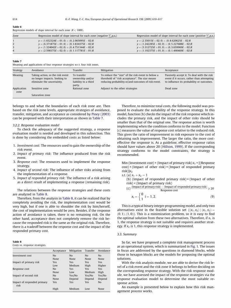
Table 6Regression models of slope interval for each zone ðR 6 1000Þ.

Zone Regression model of slope interval for each zone (negativeP

ipixi) Regression model of slope interval for each zone (positiveP

ipixi)

1 y ¼ ð1:652324Eþ 01;0Þ þ ð0;2:065095E� 02ÞR y ¼ ð2:35015Eþ 02; 0Þ þ ð0;8:620625E� 02ÞR2 y ¼ ð6:371875Eþ 01;0Þ þ ð0;3:834375E� 02ÞR y ¼ ð1:242285Eþ 02;0Þ þ ð0;5:227688E� 02ÞR3 y ¼ ð1:324042Eþ 02;0Þ þ ð0;4:751344E� 02ÞR y ¼ ð5:312725Eþ 01;0Þ þ ð0;3:659969E� 02ÞR4 y ¼ ð2:598375Eþ 02;0Þ þ ð0;1:117781E� 01ÞR y ¼ ð1:192375Eþ 01;0Þ þ ð0;1:490469E� 02ÞR

Table 7Meaning and applications of four response strategies w.r.t. four risk zones.

Strategy Avoidance Transfer Mitigation Acceptance

Meaning Taking action, so the risk eventno longer impacts. Seeking toeliminate the uncertainty.

To transferownership and/orliability to a thirdparty.

To reduce the ‘‘size” of the risk event to below athreshold of ‘‘risk acceptance”. The size meansreducing probability or/and outcomes of risk event.

Passively accept it. To deal with the riskevent if it occurs, rather than attemptingto influence its probability or outcomes.

Applicationzone

Sensitive zone Rational zone Adjunct to the other strategies Dead zone

Saturation zone

614 H.-F. Wang, F.-C. Hsu / European Journal of Operational Research 198 (2009) 610–617

belongs to and what the boundaries of each risk zone are. Thenbased on the risk zone levels, appropriate strategies of avoidance,transfer, mitigation, and acceptance as considered by Piney (2003)can be proposed with their interpretation as shown in Table 7.

3.2.2. Response evaluation modelTo check the adequacy of the suggested strategy, a response

evaluation model is needed and developed in this subsection. Thisis done by considering the embedded costs as listed below:

1. Investment cost: The resources used to gain the ownership of therisk event.

2. Impact of primary risk: The influence produced from the riskevent.

3. Response cost: The resources used to implement the responsestrategy.

4. Impact of second risk: The influence of other risks arising fromthe implementation of a response.

5. Impact of responded primary risk: The influence of a risk arisingas a direct result of implementing a response (remaining risk).

The relations between the response strategies and these costsare analyzed in Table 8.

Therefore, from the analysis in Table 8, it can be realized that bycompletely avoiding the risk, the implementation cost would bevery high, but if one is able to shoulder the risk by him/herself,the cost of implementation would be zero. Besides, if the responseaction of avoidance is taken, there is no remaining risk. On theother hand, acceptance does not completely remove the risk be-cause the responded risk is the same as the original risk. Therefore,there is a tradeoff between the response cost and the impact of theresponded primary cost.

Table 8Costs vs. response strategies.

Acceptance Mitigation Transfer Avoidance

Investment cost No No No NoNone None None None

Impact of primary risk Yes Yes Yes YesLow Medium High Higher

Response cost No Yes Yes YesNone Low Medium High

Impact of second risk No Yes/No Yes/No Yes/NoNone Depend Depend Depend

Impact of responded primaryrisk

Yes Yes Yes No

High Medium Low None

Therefore, to minimize total costs, the following model was pro-posed to evaluate the suitability of the response strategy. In thismodel, function (b) checks the impact of the risk response which in-cludes the primary risk, and the impact of other risks should besmaller than that of the original one. The response action is worthimplementing when the condition conforms to the model. Function(c) measures the value of response cost relative to the reduced risk.This gives the ratio of improvement in risk exposure to the cost ofobtaining such improvement. The larger the ratio, the more cost-effective the response is. As a guideline, effective response ratiosshould have values above 20 (Hillson, 1999). If the correspondingstrategy conforms to the model constraints, the strategy isrecommended.

Min (Investment cost) + (Impact of primary risk) x1 + [(Responsecost) + (Impact of other risk) + (Impact of responded primaryrisk)]x2

s.t. (a) x1 þ x2 ¼ 1

(b) (Impact of responded primary risk) + (Impact of otherrisk) < (Impact of primary risk)

(c) ðImpact of primary riskÞ�ðImpact of responded primary riskÞResponse cost

P 20

xi ¼01

�i ¼ 1;2: ð9Þ

This is a typical binary integer programming model, and only twoalternatives exist in the feasible solution set fðx1;x2Þ j ðx1; x2Þ ¼ð0;1Þ; ð1;0Þg. This is a minimization problem, so it is easy to findthe optimal solution from these two alternatives. Therefore, if x1 is1, the response strategy is not suitable and requires another strat-egy. If x2 is 1, this response strategy is implemented.

3.3. Summary

So far, we have proposed a complete risk management processas an operational system, which is summarized in Fig. 1. The issuesin focus are addressed by the questions in diamond blocks, whilethose in hexagon blocks are the models for proposing the optimalsolutions.

With the risk analysis module, we are able to derive the risk le-vel of a risk event and the risk zone it belongs to before deciding onthe corresponding response strategy. With the risk response mod-ule, we have assessed the impact of the response strategies via theresponse evaluation model to determine the most suitable re-sponse action.

An example is presented below to explain how this risk man-agement process works.

Identify mission, aims, andobjective

Risk identification,Risk measurement, and

Risk assessment

Assess risk tolerance, R,by CE method

Personal risk zones

Which tolerance level(riskzone)?

Dead zone Sensitivezone

Saturationzone

Rationalzone

Which response strategy?

Riskacceptance

Risktransfer

Riskavoidance

Riskmitigation

Suitable?

Implementation

Other risk exists?

End

Yes

No

NoYes

Risk analysis

Risk response

Personal risk level

Response evaluation model

Fig. 1. Framework of the proposed individual risk management system.

H.-F. Wang, F.-C. Hsu / European Journal of Operational Research 198 (2009) 610–617 615

4. Illustrative example

We adopted the court case of A–C to illustrate the proposed pro-cedure and compare the result with EMV as formally suggested(Clemen and Reilly, 2001).

4.1. Problem description and analysis

This case involved two persons, A and B, who agreed to theterms of a merger. However, person C offered B a substantially bet-ter price, and B reneged on the deal with A and sold to C. Naturally,A felt if it had been dealt with unfairly and immediately filed a law-suit against C, alleging that C had legally interfered in the A–Bnegotiations. A won the case and it was awarded $10,300. C hadsaid that it would file for bankruptcy if A obtained court permis-

sion to secure the judgment by filing liens against C’s assets. Fur-thermore, C was determined to fight the case all the way to theUS Supreme Court, if necessary, arguing in part that A had not fol-lowed the security and exchange commission regulations in itsnegotiations with B. In April 1987, just before A began to file theliens, C offered to pay $2000 to A, to settle the entire case. A indi-cated that he had been advised that a settlement between $3000and $5000 would be fair.

What do you think A should do? Should he accept the offer of$2000, or should he refuse and make a counter-offer? If he refusesthe certainty of $2000, he faced with a risky situation. C may, indeed,agree to pay $5000, a reasonable amount in A’s mind. On the otherhand, if he places a counter-offer of $5000 as a settlement amount,C may perhaps counter with $3000 or simply pursue a further appeal.In Fig. 2, a decision tree shows a simplified version of A’s problem.

Counteroffer 5000

Accept 2000

C Accepts 5000

C refusescounteroffer

C counteroffers 3000

Final court decision

Final courtdecision

Refuse

Accept 3000

2000

5000

10300

5000

0

10300

5000

0

3000

Settlement Amount

(0.17)

(0.50)

(0.33)

(0.2)

(0.2)

(0.5)

(0.5)

(0.3)

(0.3)

Fig. 2. Decision tree for A–C court (Clemen and Reilly, 2001).

Settlement Amount0.2

0.5

0.3-3000

2000

7300

Fig. 3. Decision tree for Decision 1.

-2000

1000

8300

3000

Settlement Amount

30000.5

0.17

0.33

0.5

0.2

0.3

Fig. 4. Decision tree for Decision 2.

616 H.-F. Wang, F.-C. Hsu / European Journal of Operational Research 198 (2009) 610–617

This risk problem can be separated into two stages for risk anal-ysis. The first is that if C counters with $3000, what should A do?The other is, should A refuse the offer and make a counter-offer?A’s risk tolerance is 1000 and is thus regarded as a risk averter.We can evaluate this risk problem using our proposed RMP, whichis as follows.

Using the interval regression results of Table 6, we can predictthe interval of slope for risk tolerance = 1000 as follows:

See Table 9

� Risk analysis:1. Decision 1

The stage 1 arrangement can be viewed in Fig. 3.Based on Eq. (5), the value of risk level V 0 ¼ 1:42E� 02 fallsin the saturation zone (zone 4); thus, the correspondingstrategy is avoidance.

2. Decision 2The stage 2 arrangement can be viewed in Fig. 4.Based on Eq. (5), the value of risk level V 0 ¼ 6:06E� 03 againfalls within the saturation zone (zone 4) so the correspond-ing strategy is avoidance. This means that A should not makea counter-offer to C and should accept the alternative of$2000.

� Risk response:

Min ðinvest cost¼0Þþðimpact of primary risk¼2120Þx1

þ½ðresponse cost¼0Þþðimpact of other risk¼0Þþðimpact of responded primary risk¼0Þ�x2

s:t: ð1Þx1þx2¼1ð2Þðimpact of responded primary risk¼0Þþðimpact of other risk¼0Þ< ðimpact of primary risk¼2120Þ

xi ¼01

�i¼1;2

The response evaluation model solution is x1 ¼ 0; x2 ¼ 1, whichsuggests that the avoidance strategy is appropriate. Therefore,

Table 9The interval of slope for risk tolerance = 1000.

PositiveP

ipixi

Zone 1 Zone 2

Upper bound Lower bound Upper bound Lower bound

3.2122E+02 1.4881E+02 1.7651E+02 7.1952E+01

according to our risk management process (IRM), we suggest thatA accept C’s offer of $2000 and forgets about making a counter-offerto C.

Zone 3 Zone 4

Upper bound Lower bound Upper bound Lower bound

8.9727E+01 1.6528E+01 2.6828E+01 �2.9809E+00

Table 10Tolerance analysis.

Zone 1 Zone 2 Zone 3 Zone 4

Range of risk tolerance �2376 2376 � 1451 1451 � 799 799 � 0Belonging zone Dead zone Rational

zoneSensitivezone

Saturationzone

Corresponding strategy Acceptance Transfer Avoidance Avoidance

H.-F. Wang, F.-C. Hsu / European Journal of Operational Research 198 (2009) 610–617 617

4.2. Discussion and conclusion

For comparison, let us use the EMV method to make the deci-sion, we obtain the result shown below:

1. Decision 1

EMV ¼ ð0:2� 10300Þ þ ð0:5� 5000Þ þ ð0:3� 0Þ ¼ 4560) 4560 > 3000* reject the alternative of Accept $300000:

2. Decision 2

EMV ¼ ð0:17� 5000Þ þ ð0:5� 4560Þ þ ð0:33� 4560Þ ¼ 4630) 4630 > 2000* reject the alternative of Accept $200000:

Therefore, A should turn down C’s offer but place a counter-of-fer for a settlement of $5000. If C turns down the $5000 and makesanother counter-offer of $3000, A should refuse the $3000 and takehis chance in court.

To compare these two risky decision methods, we offer the fol-lowing conclusions:

1. IRM is analyzed according to an individual’s risk attitude,whereas EMV is applied for types of individuals and thus therecommended action will be the same for each one.

2. In this case, A is a risk averter. According to our analysis, thisrisk event was at a high level of risk (sensitive zone) for A.Therefore, we recommended A to implement the responsestrategy of ‘‘Avoidance” and accept the offer from C becausethe response cost is the minimum. This result matches our com-mon knowledge, yet different from that suggested by EMV.Now,using the regression model, we further analyzed the toleranceranges for this case as shown in Table 10.

5. Conclusion

An operational risk management system is an essential tool indecision making, which helps evaluate the influence of a risk in astep by step manner. The more precise the analysis process, themore appropriate is the response action recommended.

Since different people may evaluate the same event as havingdifferent levels of risk, in this study, we explored risk tolerancebased on individual preferences. To develop a complete analysisof risk management, we studied and proposed a risk managementmodule called individual risk management by adopting the cumu-lative prospect theory to describe individual preferences, and usedthe slope as a measure to separate individual risk levels when thec-means clustering method was used. To perform tolerance analy-sis, we examined the clustering results to discover the relation be-tween risk tolerance and risk level. After these analyses, riskresponse strategies based on the properties of the four risk zones

were considered. Acceptance of the recommended strategy wasbased on the proposed evaluation model, which assessed the re-sponse strategies based on the overall costs of both operationand impact embedded in the implemented results.

IRM has shown to provide more precise assessment at the riskanalysis stage, and consider more thorough evaluation factors atthe risk response stage. This is a systematic process which includesfollow-up consideration in assessing risks and response and pro-vides more useful information for coping with the risks one faces.In addition, we solved the division problem of Piney’s four riskzones using the clustering method. Therefore, the guidelines out-lined in this paper offer a framework for developing effective riskanalysis and response, and for minimizing the influence resultingfrom such risk.

Acknowledgement

The authors acknowledge the financial support from the Na-tional Science Council with Project Number NSC 93-2213-E007-016.

References

Alexander, C., Sheedy, E., 2004. The Professional Risk managers’ Handbook: AComprehensive Guide to Current Theory and Best Practices, first ed. PRMIAPublications, Wilmington, DE.

Bleichrodt, H., Pinto, J.L., 2000. A parameter-free elicitation of the probabilityweighting function in medical decision analysis. Management Science 46 (11),1485–1496.

Borodzicz, Edward P., 2005. Risk, Crisis and Security Management. John Wiley andSons Ltd., West Sussex, England.

Chateauneuf, A., Wakker, P., 1999. An axiomatization of cumulative prospect theoryfor decision under risk. Journal of Risk and Uncertainty 18 (2), 137–145.

Clemen, R.T., Reilly, T., 2001. Making Hard Decisions with Decision Tools. Duxbury,Belmont, California.

Crockford, Neil, 1986. An Introduction to Risk Management, second ed. Woodhead-Faulkner. 0-85941-332-2.

Fennema, H., Wakker, P., 1997. Original and cumulative prospect theory: A discussionof empirical differences. Journal of Behavioral Decision Making 10, 53–64.

Fishburn, P.C., 1982. The Foundations of Expected Utility. Reidel, Dordrecht Holland.Goicoechea, A., Hansen, D.R., Duckstein, L., 1982. Multiobjective Decision Analysis

with Engineering and Business Applications. John Wiley, New York.Hillson, D. 1999. Developing effective risk responses. In: Proceedings of the 30th

Annual Project Management Institute 1999 Seminar and SymposiumPhiladelphia, Pennsylvania, USA, Papers presented October 10–16.

Hojati, M., Bector, C.R., Smimou, K., 2005. A simple method for computation of fuzzylinear regression. European Journal of Operational Research 166, 172–184.

Kahneman, D., Tversky, A., 1979. Prospect theory: An analysis of decision under risk.Econometrica 47 (2), 263–292.

Kaufman, L., Rousseeuw, P.J., 1990. Finding Groups in Data: An Introduction toCluster Analysis. John Wily & Sons, New York.

Lee, H., Tanaka, H., 1999. Upper and lower approximation models in intervalregression using regression quantile techniques. European Journal ofOperational Research 116, 653–666.

Levy, H., 2006. Stochastic Dominance, second ed.. Investment Decision Makingunder Uncertainty Springer, USA.

Neilson, W., Stowe, J., 2002. A further examination of cumulative prospect theoryparameterizations. The Journal of Risk and Uncertainty 24 (1), 31–46.

Piney, C., 2003. Applying utility theory to risk management. Project ManagementJournal 34 (3), 26–31.

Prelec, D., 1998. The probability weighting function. Econometrica 66 (3), 497–527.Tummala, V.M.R., Burchett, J.F., 1999. Applying a risk management process (RMP) to

manage cost risk for an EHV transmission line project. International Journal ofProject Management 17 (4), 223–235.

Tummala, V.M. R., Leung, Y.H., 1996. A risk management model to assess safety andreliability risks. International Journal of Quality and Reliability Management 13(8), 53–62.

Tversky, A., Kahneman, D., 1992. Advanced in prospect theory: Cumulativerepresentation of uncertainty. Journal of Risk and Uncertainty 5 (4), 297–323.

Von Neumann, J., Morgenstern, O., 2004. Theory of Games and Economic Behavior.Princeton University Press, New Work.

Ward, D., Quaid, C., 2007. The pursuit of courage, judgment and luck. Special issue ofRogue Risk Rant, Mar/Apr, Journal of Defense Acquisition, Technology andLogistics (AT&L), Defense Acquisition University.

Wu, G., Gonzalez, R., 1996. Curvature of the probability weighting function.Management Science 42, 1676–1690.