an introduction to basic statistics and probability

An Introduction to Basic Statisticsand Probability

Shenek Heyward

NCSU

An Introduction to Basic Statistics and Probability – p. 1/40

Outline

Basic probability concepts

Conditional probability

Discrete Random Variables and Probability Distributions

Continuous Random Variables and ProbabilityDistributions

Sampling Distribution of the Sample Mean

Central Limit Theorem


Idea of Probability

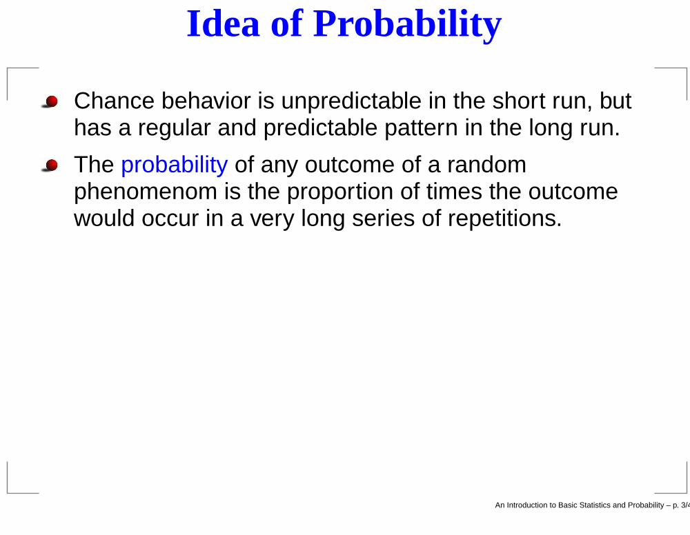
Chance behavior is unpredictable in the short run, buthas a regular and predictable pattern in the long run.

The probability of any outcome of a randomphenomenom is the proportion of times the outcomewould occur in a very long series of repetitions.


Terminology

Sample Space - the set of all possible outcomes of arandom phenomenon

Event - any set of outcomes of interest

Probability of an event - the relative frequency of thisset of outcomes over an infinite number of trials

Pr(A) is the probability of event A


Example

Suppose we roll two die and take their sum

S = {2, 3, 4, 5, .., 11, 12}Pr(sum = 5) = 4

36

Because we get the sum of two die to be 5 if we roll a(1,4),(2,3),(3,2) or (4,1).


Notation

Let A and B denote two events.A ∪ B is the event that either A or B or both occur.A ∩ B is the event that both A and B occursimultaneously.

The complement of A is denoted by A.

A is the event that A does not occur.Note that Pr(A) = 1 − Pr(A).


Definitions

A and B are mutually exclusive if both cannot occur atthe same time.

A and B are independent events if and only if

Pr(A ∩ B) = Pr(A) Pr(B).


Laws of Probability

Multiplication Law: If A1, · · · , Ak are independentevents, then

Pr(A1 ∩ A2 ∩ · · · ∩ Ak) = Pr(A1) Pr(A2) · · ·Pr(Ak).

Addition Law: If A and B are any events, then

Pr(A ∪ B) = Pr(A) + Pr(B) − Pr(A ∩ B)

Note: This law can be extended to more than 2 events.


Conditional Probability

The conditional probability of B given A

Pr(B|A) =Pr(A ∩ B)

Pr(A)

A and B are independent events if and only if

Pr(B|A) = Pr(B) = Pr(B|A)


Random Variable

A random variable is a variable whose value is anumerical outcome of a random phenomenon

Usually denoted by X, Y or Z.

Can beDiscrete - a random variable that has finite orcountable infinite possible values

Example: the number of days that it rains yearlyContinuous - a random variable that has an(continuous) interval for its set of possible values

Example: amount of preparation time for the SAT


Probability Distributions

The probability distribution for a random variable Xgives

the possible values for X, andthe probabilities associated with each possible value(i.e., the likelihood that the values will occur)

The methods used to specify discrete prob.distributions are similar to (but slightly different from)those used to specify continuous prob. distributions.


Probability Mass Function

f(x) - Probability mass function for a discrete randomvariable X having possible values x1, x2, · · ·f(xi) = Pr(X = xi) is the probability that X has thevalue xi

Properties0 ≤ f(xi) ≤ 1∑

i f(xi) = f(x1) + f(x2) + · · · = 1

f(xi) can be displayed as a table or as a mathematicalfunction


Probability Mass Function

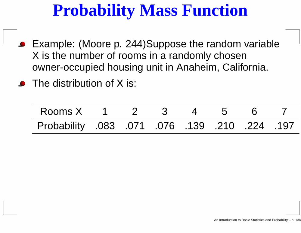
Example: (Moore p. 244)Suppose the random variableX is the number of rooms in a randomly chosenowner-occupied housing unit in Anaheim, California.

The distribution of X is:

Rooms X 1 2 3 4 5 6 7Probability .083 .071 .076 .139 .210 .224 .197


Parameters vs. Statistics

A parameter is a number that describes the population.Usually its value is unknown.

A statistic is a number that can be computed from thesample data without making use of any unknownparameters.

In practice, we often use a statistic to estimate anunknown parameter.


Parameter vs. Statistic Example

For example, we denote the population mean by µ, andwe can use the sample mean x̄ to estimate µ.

Suppose we wanted to know the average income ofhouseholds in NC.

To estimate this population mean income µ, we mayrandomly take a sample of 1000 households andcompute their average income x̄ and use this as anestimate for µ.


Expected Value

Expected Value of X or (population) mean

µ = E(X) =R

∑

i=1

xi Pr(X = xi) =R

∑

i=1

xif(xi),

where the sum is over R possible values. R may befinite or infinite.

Analogous to the sample mean x̄

Represents the "average" value of X


Variance

(Population) variance

σ2 = V ar(X)

=R

∑

i=1

(xi − µ)2 Pr(X = xi)

=R

∑

i=1

x2

i Pr(X = xi) − µ2

Represents the spread, relative to the expected value,of all values with positive probability

The standard deviation of X, denoted by σ, is thesquare root of its variance.


Room Example

For the Room example, find the following

E(X)

V ar(X)

Pr [a unit has at least 5 rooms]


Binomial Distribution

StructureTwo possible outcomes: Success (S) and Failure (F).Repeat the situation n times (i.e., there are n trials).The "probability of success," p, is constant on eachtrial.The trials are independent.


Binomial Distribution

Let X = the number of S’s in n independent trials.(X has values x = 0, 1, 2, · · · , n)

Then X has a binomial distribution with parameters nand p.

The binomial probability mass function is

Pr(X = x) =

(

n

x

)

px(1 − p)n−x, x = 0, 1, 2, · · · , n

Expected Value: µ = E(X) = np

Variance: σ2 = V ar(X) = np(1 − p)


Example

Example: (Moore p.306) Each child born to a particularset of parents has probability 0.25 of having blood typeO. If these parents have 5 children, what is theprobability that exactly 2 of them have type O blood?

Let X= the number of boys

Pr(X = 2) = f(2) =

(

5

2

)

(.25)2(.75)3 = .2637


Example

What is the expected number of children with type Oblood?µ = 5(.25) = 1.25

What is the probability of at least 2 children with type Oblood?

Pr(X ≥ 2) =5

∑

k=2

(

5

k

)

(.25)k(.75)5−k

= 1 −1

∑

k=0

(

5

k

)

(.25)k(.75)5−k

= .3671875


Continuous Random Variable

f(x) - Probability density function for a continuousrandom variable X

Propertiesf(x) ≥ 0∫

∞

−∞f(x)dx = 1

P [a ≤ X ≤ b] =∫ ba f(x)dx

Important Notes

P [a ≤ X ≤ a] =∫ aa f(x)dx = 0

This implies that P [X = a] = 0

P [a ≤ X ≤ b] = P [a < X < b]


Summarizations

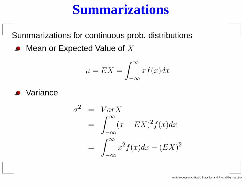
Summarizations for continuous prob. distributions

Mean or Expected Value of X

µ = EX =

∫

∞

−∞

xf(x)dx

Variance

σ2 = V arX

=

∫

∞

−∞

(x − EX)2f(x)dx

=

∫

∞

−∞

x2f(x)dx − (EX)2


Example

Let X represent the fraction of the population in acertain city who obtain the flu vaccine.

f(x) =

{

2x when 0 ≤ x ≤ 1,

0 otherwise.

Find P(1/4 ≤ X ≤ 1/2)

P (1/4 ≤ X ≤ 1/2) =

∫

1/2

1/4

f(x)dx

=

∫

1/2

1/4

2xdx

= 3/16An Introduction to Basic Statistics and Probability – p. 25/40

Example

f(x) =

{

2x when 0 ≤ x ≤ 1,

0 otherwise.

Find P(X ≥ 1/2)

Find EX

Find V arX


Normal Distribution

Most widely used continuous distribution

Also known as the Gaussian distribution

Symmetric


Normal Distribution

Probability density function

f(x) =1

σ√

2πexp

[

−(x − µ)2

2σ2

]

EX = µ

V arX = σ2

Notation: X ∼ N(µ, σ2)means that X is normally distributed with mean µ andvariance σ2.


Standard Normal Distribution

A normal distribution with mean 0 and variance 1 iscalled a standard normal distribution.

Standard normal probability density function

f(x) =1√2π

exp

[−x2

2

]

Standard normal cumulative probability functionLet Z ∼ N(0, 1)

Φ(z) = P (Z ≤ z)

Symmetry property

Φ(−z) = 1 − Φ(z)


Standardization

Standardization of a Normal Random Variable

Suppose X ∼ N(µ, σ2) and let Z = X−µσ . Then

Z ∼ N(0, 1).

If X ∼ N(µ, σ2), what is P (a < X < b)?Form equivalent probability in terms of Z :

P (a < X < b) = P

(

a − µ

σ< Z <

b − µ

σ

)

Use standard normal tables to compute latterprobability.


Standardization

Example. (Moore pp.65-67) Heights of Women

Suppose the distribution of heights of young women arenormally distributed with µ = 64 and σ2 = 2.72 What isthe probability that a randomly selected young womanwill have a height between 60 and 70 inches?

Pr(60 < X < 70) = Pr

(

60 − 64

2.7< Z <

70 − 64

2.7

)

= Pr(−1.48 < Z < 2.22)

= Φ(2.22) − Φ(−1.48)

= .9868 − .0694

= .9174


Sampling Distribution of X

A natural estimator for the population mean µ is thesample mean

X =n

∑

i=1

Xi

n.

Consider x to be a single realization of a randomvariable X over all possible samples of size n.

The sampling distribution of X is the distribution ofvalues of x over all possible samples of size n that couldbe selected from the population.


Expected Value ofX

The average of the sample means (x’s) when takenover a large number of random samples of size n willapproximate µ.

Let X1, · · · , Xn be a random sample from somepopulation with mean µ. Then for the sample mean X,

E(X) = µ.

X is an unbiased estimator of µ.


Standard Error of X

Let X1, · · · , Xn be a random sample from somepopulation with mean µ. and variance σ2.

The variance of the sample mean X is given by

V ar(X) = σ2/n.

The standard deviation of the sample mean is given byσ/

√n. This quantity is called the standard error (of the

mean).


Standard Error of X

The standard error σ/√

n is estimated by s/√

n.

The standard error measures the variability of samplemeans from repeated samples of size n drawn from thesame population.

A larger sample provides a more precise estimate X ofµ


Sampling Distribution of X

Let X1, · · · , Xn be a random sample from a populationthat is normally distributed with mean µ and variance σ2.

Then the sample mean X is normally distributed withmean µ and variance σ2/n.

That isX ∼ N(µ, σ2/n).


Central Limit Theorem

Let X1, · · · , Xn be a random sample from anypopulation with mean µ and variance σ2.

Then the sample mean X is approximately normallydistributed with mean µ and variance σ2/n.


Data Sampled from Uniform Distribution

The following is a distribution of X when we take samplesof size 1.


Example

The following is a distribution of X when we take samplesof size 10.


References

Moore, David S., "The Basic Practice of Statistics."Third edition. W.H. Freeman and Company. New York.2003

Weems, Kimberly. SIBS Presentation, 2005.


an introduction to basic statistics and probability

Documents