ETHIOPIAN DEVELOPMENT RESEARCH INSTITUTE

An Introduction to Data Fusion for Ethiopian Agricultural Research: Incorporating Remote Sensing, GIS, and Spatial Estimation Techniques for Enhanced Analysis

Authors:James Warner—IFPRI—Addis Ababa (j.warner@cigar.org)Michael Mann—George Washington University (mmann1123@email.gwu.edu)Leulsegged Kasa—IFPRI—Addis Ababa (l.kasa@cigar.org)

Ethiopian Economics Association 13th International Conference on the Ethiopian EconomyJuly 23-25, 2015Addis Ababa

1

2

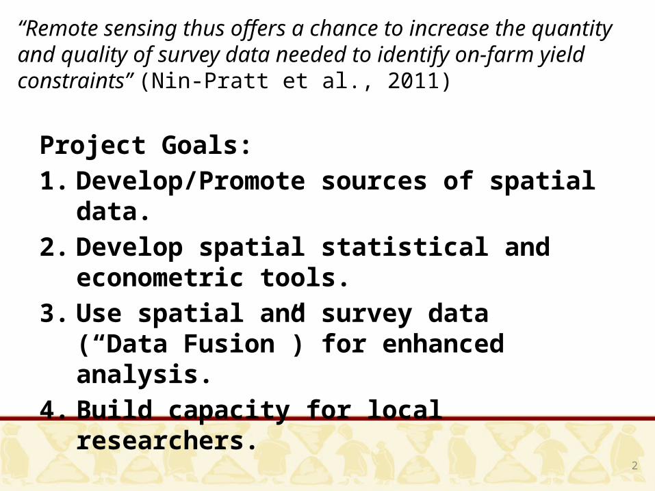
“Remote sensing thus offers a chance to increase the quantity and quality of survey data needed to identify on-farm yield constraints” (Nin-Pratt et al., 2011)

Project Goals:1. Develop/Promote sources of spatial data. 2. Develop spatial statistical and econometric tools.3. Use spatial and survey data (“Data Fusion”) for

enhanced analysis.4. Build capacity for local researchers.

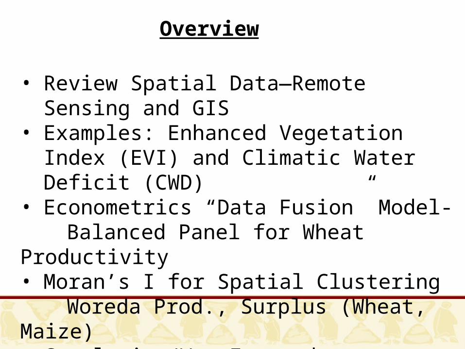
• Review Spatial Data—Remote Sensing and GIS• Examples: Enhanced Vegetation Index (EVI) and

Climatic Water Deficit (CWD)• Econometrics “Data Fusion” Model-

Balanced Panel for Wheat Productivity • Moran’s I for Spatial Clustering

Woreda Prod., Surplus (Wheat, Maize)• Conclusion/Way Forward

Overview

DataPrimary data sources

Remote Sensing• Temperature

• Greenness (EVI)• Elevation• Rainfall

• Long Term S/D Rainfall (CWD)

Geographic Information Systems• Administrative boundaries

(shapefiles)• Travel times via road networks• Terrain slope, aspect• Road density

Survey Data• Agricultural Sample Survey (AgSS)• 2007 Population Census

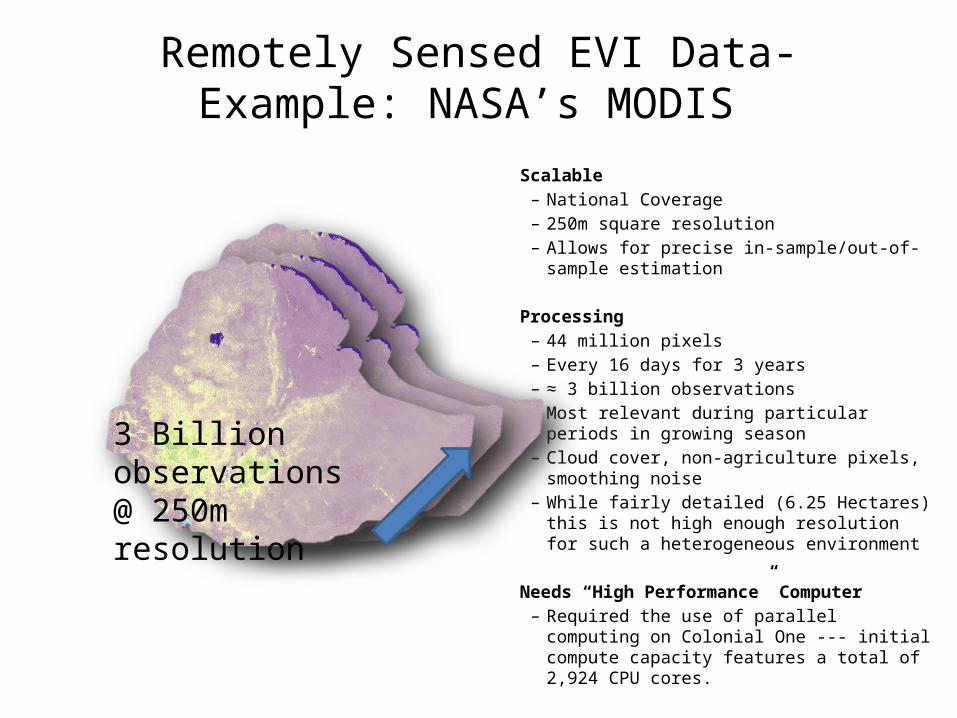
Remotely Sensed EVI Data-Example: NASA’s MODIS

Scalable– National Coverage– 250m square resolution– Allows for precise in-sample/out-of-sample

estimation

Processing– 44 million pixels– Every 16 days for 3 years– ≈ 3 billion observations– Most relevant during particular periods in

growing season– Cloud cover, non-agriculture pixels,

smoothing noise – While fairly detailed (6.25 Hectares) this is

not high enough resolution for such a heterogeneous environment

Needs “High Performance” Computer– Required the use of parallel computing on

Colonial One --- initial compute capacity features a total of 2,924 CPU cores.

3 Billion observations@ 250m resolution

Enhanced Vegetation Index (EVI)

Sensitive the amount of chlorophyll in any given pixel (greenness)

Proxy for:• Plant health• Water availability during

critical growth periods

Correlates well with:• Plant productivity• Crop yields

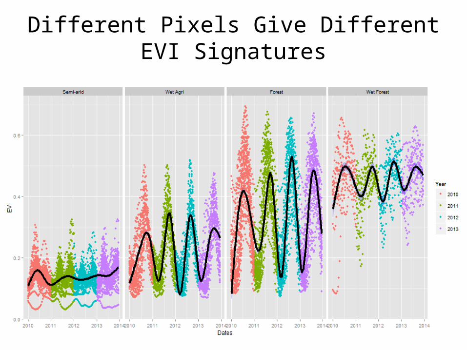
Different Pixels Give Different EVI Signatures

Enhanced Vegetation Index (EVI)

EVI Area Under the Curve (Decreasing from max— “Grain Filling”)

Water availability and plant health at critical periods• head development• yield formation

Meher Rainy

Season

Harvest

This is a generalization (but you get the point)

Start of rainy season the first ten day period that accounts for 2.5% of total annual rainfall, and that is followed by a 30 day period that experiences no more than 7 consecutive days without rain

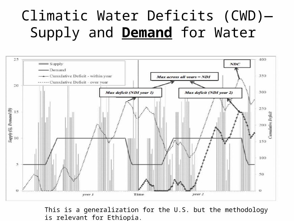
Climatic Water Deficits (CWD)—Supply and Demand for Water

This is a generalization for the U.S. but the methodology is relevant for Ethiopia.

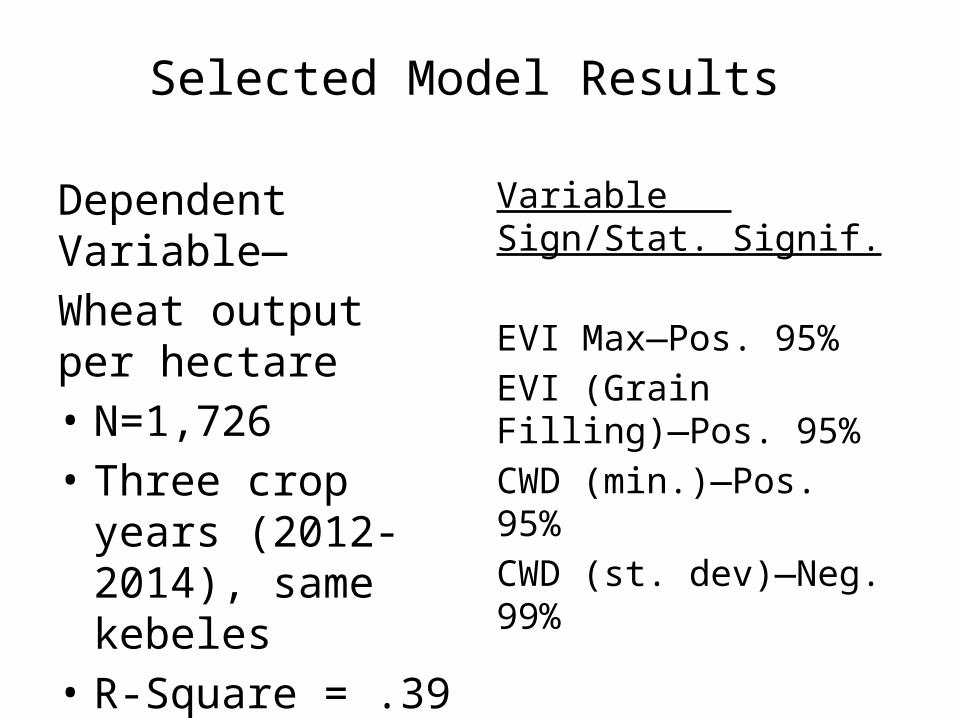
Selected Model Results

Dependent Variable—Wheat output per hectare • N=1,726• Three crop years

(2012-2014), same kebeles

• R-Square = .39

Variable Sign/Stat. Signif.

EVI Max—Pos. 95%EVI (Grain Filling)—Pos. 95%CWD (min.)—Pos. 95%CWD (st. dev)—Neg. 99%

Moran’s I—Spatial AutocorrelationWeighted Index—Correlation and the inverse of the distance

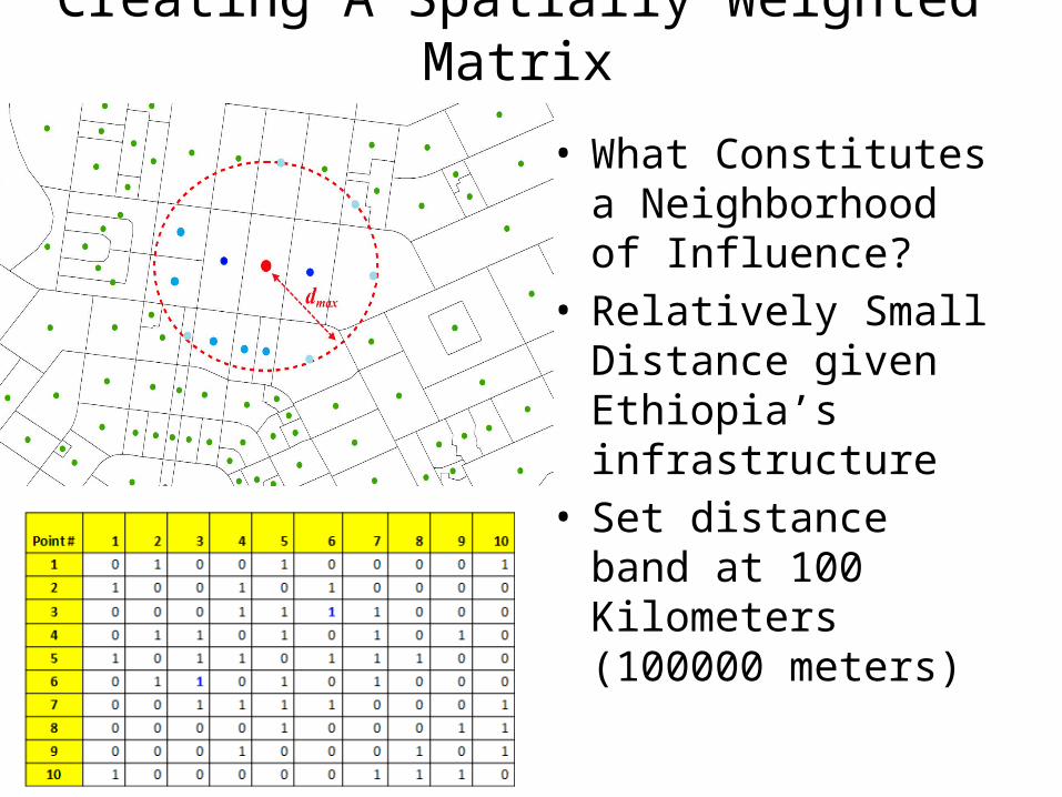
Creating A Spatially Weighted Matrix

• What Constitutes a Neighborhood of Influence?

• Relatively Small Distance given Ethiopia’s infrastructure

• Set distance band at 100 Kilometers (100000 meters)

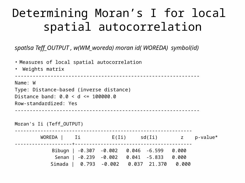
Determining Moran’s I for local spatial autocorrelation

spatlsa Teff_OUTPUT , w(WM_woreda) moran id( WOREDA) symbol(id) • Measures of local spatial autocorrelation• Weights matrix--------------------------------------------------------------Name: WType: Distance-based (inverse distance)Distance band: 0.0 < d <= 100000.0Row-standardized: Yes-------------------------------------------------------------- Moran's Ii (Teff_OUTPUT)-------------------------------------------------------------- WOREDA | Ii E(Ii) sd(Ii) z p-value*--------------------+----------------------------------------- Bibugn | -0.307 -0.002 0.046 -6.599 0.000 Senan | -0.239 -0.002 0.041 -5.833 0.000 Simada | 0.793 -0.002 0.037 21.370 0.000

Maize Production-Woreda Clustering

Moran’s I (4 year Avg.)Change= ((2014 + 2013)-(2012 -2011))/sd(I)

Major clusters in Amhara and Oromia regions: West Gojam and East Wellega zones. Strengthening in East Wellega and northern SNNP.

Wheat Production—Woreda Clustering

Moran’s I (4 year Avg.)Change= ((2014 + 2013)-(2012 -2011))/sd(I)

The principal cluster is Oromia: Arsi, Bale, and West Arsi zones and seems to be strengthening in Arsi and Bale.

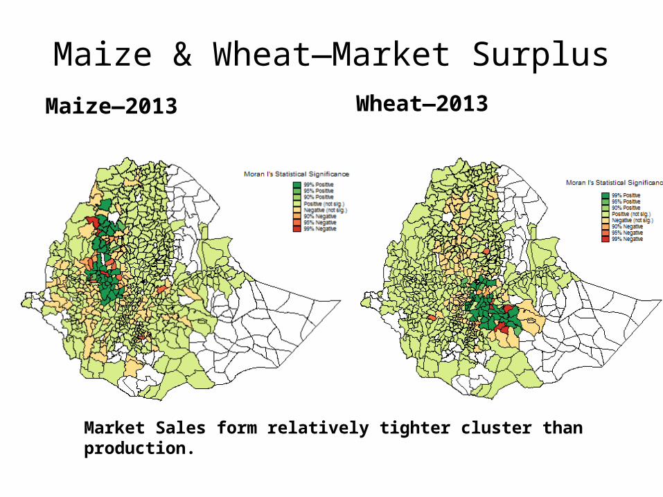
Maize & Wheat—Market SurplusMaize—2013 Wheat—2013

Market Sales form relatively tighter cluster than production.

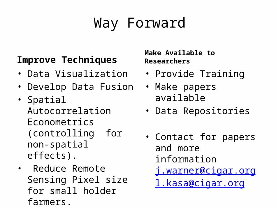
Way Forward

Improve Techniques• Data Visualization• Develop Data Fusion• Spatial Autocorrelation

Econometrics (controlling for non-spatial effects).

• Reduce Remote Sensing Pixel size for small holder farmers.

Make Available to Researchers

• Provide Training• Make papers available• Data Repositories

• Contact for papers and more information j.warner@cigar.org l.kasa@cigar.org