an introduction to error correcting codes...
TRANSCRIPT

AN INTRODUCTION TO AN INTRODUCTION TO ERROR CORRECTING ERROR CORRECTING
CODESCODESPart 2Part 2
Jack Keil Wolf
ECE 154 CSpring 2010

BINARY CONVOLUTIONAL CODES
• A binary convolutional code is a set of infinite lengthbinary sequences which satisfy a certain set of conditions. In particular the sum of two code words is a code word.
• It is easiest to describe the set of sequences in terms of a convolutional encoder that produces these sequences. However for a given code, the encoder is not unique.
• We start with a simple example.

A RATE ½, 4-STATE, BINARY CONVOLUTIONAL ENCODER
• Consider the 4-state, binary, convolutional encoder shown below:
• There are two output binary digits for each (one) input binary digit. This gives a rate ½ code.
• Each adder adds its two inputs modulo 2.
Input
Binary Sequence
Output
Binary Sequence
⊕ ⊕
⊕

A RATE ½ ENCODER• Consider the following encoder.
• Assume current state is 1 0 and input is a 1.• Then, the next state is 1 1.• The outputs are 0 1.
Input 1 Output 0 1
⊕ ⊕
⊕
0
1Current state 1 0
Next state 11
1 0

A RATE ½ ENCODER• The output code words are the labels on the branches of all of
the paths through the binary tree. The nodes in the tree are the states of the encoder. Assume we start in the 00 state.
Input 0
Input 1
0 0
1 1
0 0
1 1
1 0
0 1
0 0
1 1
1 0
0 11 1
0 0
0 1
1 0
00
00
00
10
10
01
11
00
10
01
1100
10
01
11

A RATE ½ ENCODER• Consider the input sequence 0 1 0 . . .
• Then the output sequence would be 0 0 1 1 1 0 . . .
Input 0
Input 1
0 0
1 1
0 0
1 1
1 0
0 1
0 0
1 1
1 0
0 11 1
0 0
0 1
1 0

NOTION OF STATES• At any time the encoder can be in one of 4 states:
s1 s0
a 0 0b 1 0c 0 1d 1 1
Input Output
⊕ ⊕
⊕
S1 S0
State

NOTION OF STATES• These states can be put as labels of the
nodes on the tree.
Input 0
Input 1
0 0
1 1
0 0
1 1
1 0
0 1
0 0
1 1
1 0
0 11 1
0 0
0 1
1 0
a
a
a
b
b
c
d
a
b
d
b
c
d
a
1 1
0 0a
b
c 0 01 1 a
b

NOTION OF A TRELLIS• There are only 4 states. Thus, the states at
the same depth in the tree can be merged, and the tree can be redrawn as a trellis:
0 0
1 1
0 0
1 1
1 00 1
0 0
1 1
1 0
0 1
1 00 1
0 0
1 1
0 0
1 1
1 0
0 1
1 00 1
0 0
1 1
a a a
b b b b
a
ccc
d d d
a

OTHER EXAMPLES• An 8-state rate ½ code
⊕ ⊕
⊕ ⊕
States000100010110001101011111
Can represent the tap connections as:Top – 1 0 1 1Bottom – 1 1 0 1.
This is written in octal as:(1,3) or (1,5).
8-state trellis

OTHER EXAMPLES• An 8-state, rate 2/3 encoder with 2 inputs and 3
outputs.
• The trellis has 8 states but 4 branches coming out of each state. There are three output binary digits on each branch. TRY DRAWING IT!!!
⊕ ⊕
⊕⊕2 inputs3 Outputs

ENCODING ON THE RATE ½, 4-STATE TRELLIS
• The path corresponding to the input 0 1 0 1 . . . is shown as the dark line and corresponds to the output 0 0 1 1 1 0 0 0 . . .
0 0
1 1
0 0
1 1
1 00 1
0 0
1 1
1 0
0 1
1 0
0 1
0 0
1 1
0 0
1 1
1 0
0 1
1 00 1
0 01 1

HARD DECISION DECODING ON THE RATE ½, 4-STATE TRELLIS
• Assume that we receive 0 1 1 1 1 0 0 0 . . . We put the number of differences or “errors” on each branch.
0 0 / 1
1 1 / 1
0 0 / 2
1 1 / 0
1 0 / 10 1 / 1
0 0 / 1
1 1 / 1
1 0 / 0
0 1 / 2
1 0/ 00 1 / 2
0 0 / 11 1 / 1
0 0 / 0
1 1 / 2
1 0 / 1
0 1 / 1
1 0 / 10 1 / 1
0 0 / 01 1 / 2

VITERBI DECODING
• We count the total number of errors on each possible path and choose the path with the fewest errors. We do this one step at a time.
1
1
2
0
11
1
1
0
2
02
11
0
2
1
1
11
02
1
1
3
1
2
2
4 or 3
4 or 3
1or 4
3 or 2

VITERBI DECODING• Viterbi decoding tells us to choose the
smallest number at each state and eliminatethe other path:
1
1
2
0
11
0
0
11
0
2
1
1
11
02
1
1
3
1
2
2
3
3
1
2
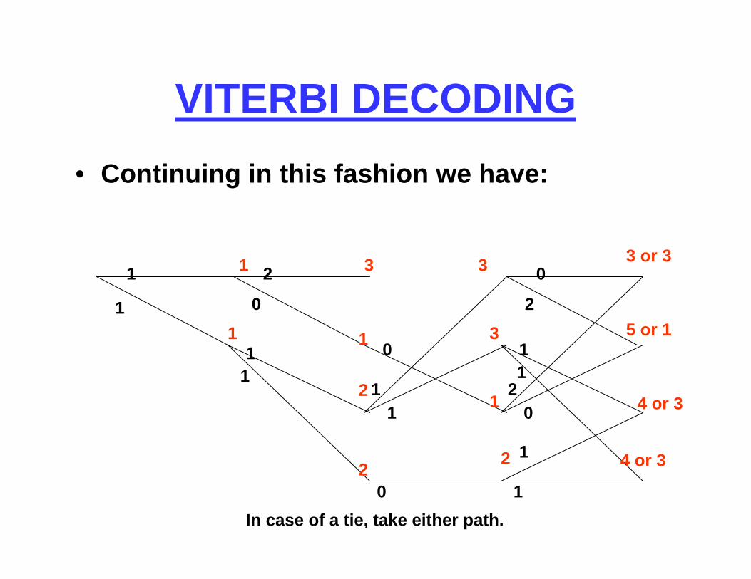
VITERBI DECODING• Continuing in this fashion we have:
1
1
2
0
11
0
0
11
0
2
1
1
11
02
1
1
3
1
2
2
3
3
1
2
3 or 3
5 or 1
4 or 3
4 or 3
In case of a tie, take either path.

VITERBI DECODING• This yields:
1
1
2
0
11
0
0
11
0
1
1
0
1
1
3
1
2
2
3
3
1
2
3
1
3
3

VITERBI DECODING• If a decision is to be made at this point we choose
the path with the smallest sum. The information sequence (i.e., input to the encoder) 0 1 0 1 corresponds to that path.
3
1
3
3
0
1
0 1

VITERBI DECODING• In a packet communication system, one
could append 0’s at the end of the message (i.e., the input to the encoder) to force the encoder back to the all 0 state.
• Then we would have only one path remaining and that would be the winning code word.

VITERBI DECODING• The basic decoding module is referred to as an ACS
module: Add, Compare, Select.
• At the decoder, one could make early decisions on the information bits by tracing back from the state with the lowest accumulated sum and then decoding some D steps back from the point of trace-back in the trellis.
. . .Winning node.Start traceback here.
Decode this branch

VITERBI DECODING• A great deal is known about how to choose D
without losing much in performance.
• In a rate ½ code, a good value of D is about 4 to 5 times the number of delay elements in the decoder.

VITERBI DECODING• The trace-back is complicated and may be the speed
“bottleneck” in the decoder.
• One may not want to trace back at each step in the trellis but rather wait for L steps and then decode L branches at a time.
• Other tricks are used in designing the decoder. One is to use a circular buffer.

DECODING ON THE TRELLIS: SOFT INPUT DECODING
• For a soft input decoder, the input to the decoders are probabilities of the code symbols.
• In actuality we use the logarithm of the probabilities so that for independent noise, the logarithm of the probability of a sequence is the sum of the logarithms of the individual symbols.
• FOR a AWGN channel, this corresponds to taking the squared difference between the noiseless transmitted outputs and the received values.

SOFT INPUT DECODING• Assume we transmit a code symbol 0 as a -1 and a
code symbol 1 as a +1. Then we would label the branches in the trellis with the transmitted values:
-1 -1
+1 +1
-1 -1
+1 +1
+1 -1-1 +1
-1 -1
+1 +1
+1 -1
-1 +1
+1 -1
-1 +1
-1 -1
+1 +1
-1 -1
+1 +1
+1 -1
-1 +1
+1 -1
-1 +1
-1 -1
+1 +1
a a a
b b b b
a
ccc
d d d
a

SOFT INPUT DECODING
• Now assume we receive the vector 0.9, 1.1, 0.8, 0.9, 0, 0.4, -1.2, -1.3, … We would put the following squared errors on the trellis:
-1 -1/ 8.02
+1 +1/ 0.02
-1 -1/6.85
+1 +1/0.05
+1 -1\3.65-1 +1\3.25
-1 -1/2.96
+1 +1/1.36
+1 -1/2.96
-1 +1/1.36
+1 -1/2.96-1 +1/1.36
-1 -1/2.96
+1 +1/1.36
-1 -1/0.13
+1 +1/10.13
+1 -1/4.93
-1 +1/5.33
+1 -1/4.93-1 +1/5.33
-1 -1/0.13
+1 +1/10.13
a a a
b b b b
a
ccc
d d d
a
(-1 - 0.9)2+(-1 - 1.1)2 = 8.02(+1-0.9)2 + (+1-1.1)2)=0.02

VITERBI ALGORITM WITH SOFT INPUT DECODING
• Now use the Viterbi Algorithm.
8.02
0.02
6.85
0.05
3.653.25
2.96
1.36
2.96
1.36
2.961.36
2.96
1.36
0.13
10.13
4.93
5.33
4.935.33
0.13
10.13
a a a
b b b b
a
ccc
d d d
a 8.02
0.02
14.87
8.07
3.67
3.27 Etc, etc., …
Min [(14.87+2.96),(3.67+1.36)]

DECODING ON THE TRELLIS: SOFT OUTPUT DECODING
• The Viterbi algorithm finds the path on the trellis that was most likely to have been transmitted. It makes hard decisions.
• There is another (more complicated) algorithm called the BCJR algorithm that produces soft outputs: that is, it produces the probability that each symbol is a 0 or a 1.
• The output of the BCJR algorithm then can be used as the soft input to another decoder. This is used in iterative decoding for Turbo Codes.

FREE HAMMING DISTANCE OF CONVOLUTIONAL CODES
• The error correction capability of a convolutionalcode is governed by the so-called “free Hamming distance”, dfree, of the code.
• dfree is the smallest Hamming distance between two paths in the trellis that start in a common state and end in a common state. Two candidate paths are:

FREE HAMMING DISTANCE OF CONVOLUTIONAL CODES
• Tables giving the free distance of a large number of convolutional codes exist in many textbooks. They usually list the codes in octal form.
• One very popular rate ½ code with 64 states is usually listed as: 133, 171. It has dfree= 10. In binary, after dropping the leading 0’s, this gives the tap connections: 1 0 1 1 0 1 1 and 1 1 1 1 0 0 1.
1 0 1 1 0 1 1
1 1 1 1 0 0 1

PUNCTURING CONVOLUTIONAL CODES
• Starting with a rate ½ encoder one can construct higher rate codes by a technique called puncturing.
• For example, consider the following pattern:– Input the first binary digit and transmit both output bits– Input the next binary digit and transmit only one of the two output
bits.– Input the next binary digit and transmit both output bits. – Input the next binary digit and transmit only one of the two output
bits.– Continue in this way where the odd input binary digits produce two
output bits but where the even inputs produce only one output bit.
• The result is a rate 2/3 code where we have 3 output binary digits for every two input binary digits.

PUNCTURING CONVOLUTIONAL CODES
• For example, in the 4-state trellis, if we omit the bottom output every other time, the result is:
• The X’s denote the missing bits and are ignored in decoding.
0 0
1 1
0 X
1 X
1 X0 X
0 0
1 1
1 0
0 1
1 00 1
0 0
1 1
0 X
1 X
1 X
0 X
1 X0 X
0 X
1 X
a a a
b b b b
a
ccc
d d d
a

PUNCTURING CONVOLUTIONAL CODES
• Note that the same trellis is used in decoding the original code and the punctured code.
• Puncturing lowers the dfree of the code. The best puncturing patterns were found by simulation.
• For example, for the rate ½, 64-state code we have:Rate Puncturing Pattern dfree
1/2 11, 11, 11, 11, 11, 11, 11 … 102/3 11, X1, 11, X1, 11, X1, 11 … 63/4 11, X1, 1X, 11, X1, 1X, 11 … 55/6 11, X1, 1X, X1, 1X, 11, X1 … 47/8 11, X1, X1, X1, 1X, X1, 1X … 3

TURBO CODES AND ITERATIVE DECODING

SYSTEMATIC CONVOLUTIONAL ENCODER
• A systematic convolutional encoder has one of its outputs equal to its input.
• Example of a 4-state, rate ½, encoder:
Input Outputs

PARALLEL TURBO ENCODER
• Example of a rate 1/3 Turbo encoder:
RandomInterleaver
Input
3 Outputs⊕ ⊕
⊕ ⊕

PARALLEL TURBO DECODER
RandomInterleaver
RandomDeinterleaver
Soft Output Decoder for Systematic Code
Soft Output Decoderfor Systematic Code
Many details are omitted
TURBO CODES• Codes with very few states give excellent
performance if the interleaver size is large enough.
• Serial Turbo codes also exist and give comparable performance.
• Higher rate codes can be obtained by puncturing.