an introduction to functional analysis - sv.20file.orgsv.20file.org/up1/1408_0.pdf · nita ruth....

AN INTRODUCTIONTO FUNCTIONALANALYSIS

Charles SwartzNew Mexico State UniversityLas Cruces, New Mexico

Marcel Dekker, Inc. New York Basel Hong Kong

Library of Congress Cataloging-in-Publication Data

Swartz, Charles.Functional analysis / Charles Swartz.

p. cm.Includes bibliographical references and index.ISBN 0-8247-8643-21. Functional analysis. II. Title.

QA320.S9 1992515'.7--dc2O

This book is printed on acid-free paper.

91-44028CIP

Copyright © 1992 by MARCEL DEKKER, INC. All Rights Reserved

Neither this book nor any part may be reproduced or transmitted in any form orby any means, electronic or mechanical, including photocopying, microfilming,and recording, or by any information storage and retrieval system, without per-mission in writing from the publisher.

MARCEL DEKKER, INC.270 Madison Avenue, New York, New York 10016

Current printing (last digit):10 9 8 7 6 5 4 3 2 1

PRINTED IN THE UNITED STATES OF AMERICA

TO

NITA RUTH

Preface

These notes evolved from the introductory functional analysis course

given at New Mexico State University. In the course, we attempted to

cover enough of the topics in functional analysis in depth and to give a

sufficient number of applications to give the students a feel for the subject.

Of course, the choice of topics reflects the interests and prejudices of the

author and many important and interesting topics are not covered at all.

We have given references for further study at many points. The students in

this course were assumed to have had an introductory course in point set

topology and a course in measure and integration. The text assumes a

knowledge of elementary point set topology including Tychonoffs Theorem

and the theory of nets and a background in real analysis equivalent to an

introductory course from a text such as [Ro] or [AB]; a few basic results

from complex analysis are required, especially in the sections on spectral

theory. The reader is also assumed to be familiar with Hilbert space; an

V

vi Preface

appendix supplies the basic properties of Hilbert spaces which are required.

Functional analysis is a subject which evolved from abstractions of

situations which repeatedly occurred in concrete function spaces,

differential and integral equations, calculus of variations, etc. The

abstractions have repeatedly repaid their debts to its foundations with

multitudes of applications. We have made an attempt to give at least

enough of these applications to indicate the interplay between the abstract

and the concrete and illustrate the beauty and usefulness of the subject.

The first section of the book introduces the basic properties of

topological vector spaces which will subsequently be used. In the second

section the three basic principles of functional analysis -- the Hahn-Banach

Theorem, the Uniform Boundedness Principle and the Open Mapping/

Closed Graph Theorems -- are established. Applications to such topics as

Fourier series, measure theory, summability and Schauder basis are given.

Locally convex spaces are studied in the third section. Topics such as

duality and polar topologies are discussed and applications to topics such as

Liapounoffs Theorem, the Stone-Weierstrass Theorem and the Orlicz-Pettis

Theorem are given. We do not present an exhaustive study of the

enormously large subject of locally convex spaces, but rather try to present

the most important and useful topics and particularly stress the important

special case of normed linear spaces. In the fourth section we study the

basic properties of linear operators between topological vector spaces. The

Uniform Boundedness Principle for barrelled spaces, the basic properties of

the transpose or adjoint operator, and the special classes of projection,

compact, weakly compact and absolutely summing operators are discussed.

Preface Vii

Applications to such topics as the integration of vector-valued functions,

Schwartz distributions, the Fredholm Alternative and the Dvoretsky-Rogers

Theorem are given. Finally, in section five we discuss spectral theory for

continuous linear operators. We first establish the spectral theorem for

compact symmetric operators and use this result to motivate the spectral

theorem for continuous symmetric (Hermitian) operators. A simple

straightforward proof of this version of the spectral theorem is given using

the Gelfand mapping. We derive the spectral theorem for normal operators

from basic results from Banach algebras; this affords the students an

introduction to the subject of Banach algebras. Applications to such topics

as Lomonosov's Theorem on the existence of invariant subspaces for

compact operators, Sturm-Liouville differential equations, Hilbert-Schmidt

operators and Wiener's Theorem are given.

These notes cover many of the basic topics presented in the classic

texts on functional analysis such as [TL], [Rul], [Cl], etc., although some

of the topics covered in the applications such as the Nikodym Boundedness

and Convergence Theorems, the Pettis and Bochner integrals, summability

and the Orlicz-Pettis Theorem are often not treated in introductory texts.

We do, however, include some material that is not found in the standard

introductory texts. We use the stronger notion of X convergence of

sequences and X bounded sets developed by the members of the

Katowice branch of the Mathematics Institute of the Polish Academy of

Sciences under the direction of Piotr Antosik and Jan Mikusinski to

establish versions of the Uniform Boundedness Principle which require no

completeness or barrelledness assumptions on the domain space of the

viii Preface

operators. It is shown that the general version of the Uniform Boundedness

Principle yields the classic version of the Uniform Boundedness Principle

for complete metric linear spaces as a corollary and the general Uniform

Boundedness Principle is employed to obtain a version of the Nikodym

Boundedness Theorem from measure theory where the classic version of

the Uniform Boundedness Principle is not applicable. These results are

obtained from a beautiful result due to Antosik and Mikusinski on the

convergence of the elements on the diagonal of an infinite matrix with

entries in a topological vector space. The matrix theorem can be viewed as

an abstract "sliding hump" technique and is used in many proofs in the text.

The notion of X bounded sets is also used to obtain hypocontinuity results

for bilinear maps which require no completeness or barrelledness

assumptions.

I would like to thank the many graduate students at New Mexico

State University who took the introductory functional analysis course from

me during the time that these notes were evolving into their final form and

especially Chris Stuart, who read through the final manuscript. Special

thanks go to my colleague and friend Piotr Antosik,who introduced me to

the matrix methods that are employed throughout this text, and to Valerie

Reed, who did such a superb job of translating my handwriting from the

original class notes.

Charles Swartz

Contents

Preface v

1. Topological Vector Spaces (TVS) 11. Definition and Basic Properties 32. Quasi-normed and Normed Linear Spaces (NLS) 133. Metrizable TVS 314. Bounded Sets in a TVS 375. Linear Operators and Linear Functionals 436. Quotient Spaces 597. Finite Dimensional TVS 65

II. The Three Basic Principles 718. The Hahn-Banach Theorem 73

8.1 Applications of the Hahn-Banach Theorem in NLS 778.2 Banach Limits 868.3 The Moment Problem 89

9. The Uniform Boundedness Principle (UBP) 919.1 Bilinear Maps 1059.2 The Nikodym Boundedness Theorem 1129.3 Fourier Series 1199.4 Vector-Valued Analytic Functions 1239.5 Summability 125

10. The Open Mapping and Closed Graph Theorems 13710.1 Schauder Basis 146

ix

X Contents

III. Locally Convex TVS (LCS) 15511. Convex Sets 15712. Separation of Convex Sets 16513. Locally Convex TVS 169

13.1 Normability 18213.2 Krein-Milman Theorem 184

14. Duality and Weak Topologies 18915. The Bipolar and Banach-Alaoglu Theorems 19916. Duality in NLS 20917. Polar Topologies 23118. The Mackey-Arens Theorem 23719. The Strong Topology and the Bidual 24320. Quasi-barrelled Spaces and the Topology j3*(E, E') 251

20.1 Perfect Sequence Spaces 25621. Bornological Spaces 26122. Inductive Limits 267

IV. Linear Operators 27723. Topologies on Spaces of Linear Operators 279

23.1 The Krein-Smulian Theorem 29024. Barrelled Spaces 29525. The UBP and Equicontinuity 30526. The Transpose of a Linear Operator 309

26.1 Banach's Closed Range Theorems 32526.2 The Closed Graph and Open Mapping Theorems for

LCS 33026.3 Vector Integration 33426.4 The Space of Schwartz Distributions 34726.5 The Lax-Milgram Theorem 36626.6 Distributions with Compact Support 37126.7 A Classical Theorem of Borel 379

27. Projections 38128. Compact Operators 387

28.1 Continuity Properties of Compact Operators 39728.2 Fredholm Alternative 40128.3 Factoring Compact Operators 40528.4 Projecting the Bounded Operators onto the Compact

Operators 41629. Weakly Compact Operators 42330. Absolutely Summing Operators 431

30.1 The Dvoretsky-Rogers Theorem 440

V. Spectral Theory 44131. The Spectrum of an Operator 44332. Subdivisions of the Spectrum and Examples 45133. The Spectrum of a Compact Operator 457

33.1 Invariant Subspaces and Lomonosov's Theorem 46134. Adjoints in filbert space 465

Contents xi

35. Symmetric, Hermitian and Normal Operators 46936. The Spectral Theorem for Compact Symmetric Operators 485

36.1 Hilbert-Schmidt Operators 49437. Symmetric Operators with Compact Resolvent 50138. Orthogonal Projections and the Spectral Theorem for

Compact Symmetric Operators 50939. Sesquilinear Functionals 51540. The Gelfand Map for Hermitian Operators 51941. The Spectral Theorem for Hermitian Operators 52342. Banach Algebras 533

43. Commutative Banach Algebras 54544. Banach Algebras with Involutions 55745. The Spectral Theorem for Normal Operators 567

Notation 573Appendix: Hilbert Space 575References 591Index 597

AN INTRODUCTIONTO FUNCTIONALANALYSIS

Part ITopological VectorSpaces (TVS)

1

Definition and Basic Properties

In this chapter we give the definition of a topological vector space

and develop the basic properties of such spaces.

Let X be a vector space (VS) over the field IF, where IF = IR or C.

Definition 1. (X, r) is a topological vector space (TVS) is r is a topology

on X such that:

(i) (x, y) - x + y is continuous from X x X -4 X and

(ii) (t, x) -+ tx is continuous from IF x X - X,

that is, the topology r is compatible with the algebraic structure of X.

For brevity, we often say that X is a TVS and suppress the topology r

Any topology r on X such that (X, r) is a TVS is called a vector

topology,

Proposition 2. Let (X, r) be a TVS.

4 Definition and Basic Properties

(i) If t0 E F, x0 E X then the map x -+ t0x + x0 is continuous

from X into X; if to * 0, the map is a homeomorphism

from X onto X.

(ii) If 2l is a (open) neighborhood base of 0 in X, then

x0 + 2t= {x0 + U : U E 2) is a open neighborhood base

at x0.

(iii) If U is (open), tU is open V t e IF, t * 0.

(iv) If 2l is a neighborhood base at 0 and U E 2l, then

3Ve 2t such that V+VcU.

Proof: The first part of (i) follows from Definition 1 and the fact

that joint continuity implies separate continuity. The second part follows

from the first part and the fact that the map x -+ (x - x0)/t0 is the inverse

of the map in (i).

(ii) and (iii) follow from (i), and (iv) follows from the continuity of

addition and the fact that 0 + 0 = 0.

Definition 3. A subset S c X is symmetric if x E S* -x E S (i.e.,

S = -S).

Remark 4. Note that every neighborhood U of 0 in a TVS contains a

symmetric neighborhood of 0 (take U n (-U)).

Definition 5. A subset S c X is balanced if x E S and t E F, I t 1 5 1,

tx E S (i.e., S = DS where D= {t e F : t 5 1)).

Chapter 1 5

Remark 6. Note that a balanced set is symmetric and contains 0.

Definition 7. If S c X, we set bal(S) = DS. bal(S) is the smallest

balanced set containing S and is called the balanced hull of S.

Proposition 8. Let X be a TVS.

(i) If U is a (open) neighborhood of 0, then bal(U) is a

(open) neighborhood of 0.

(ii) If S is balanced, then S is balanced.

Proof: (i) follows from Proposition 2 (iii). For (ii) note that D x S

is mapped into S by the continuous map, (t, x) -4 tx so D x S is mapped

into S and S is balanced.

Theorem 9. If 9L is a (open) neighborhood base of 0 in a TVS, X, and

Y is the family of balanced hulls of members of YC, then Y is a (open)

neighborhood base at 0. That is, 3 a base at 0 consisting of balanced

sets.

Proof: Let U e W. Since 0.0 = 0 and scalar multiplication is

continuous, 3 a (open) neighborhood of 0, Wl, whose balanced hull W2

is contained in U. Now W2 is a (open) neighborhood of 0 by

Proposition 8 so 3 U1 a V such that U1 c W2. If V = bal(U1), then

VcW2cU and VE Y.


Corollary 10. Let (X, ti) be a TVS. The following are equivalent:

(i) r is Hausdorff, i.e., (X, r) is a Hausdorff TVS.

(ii) (0} = (0)

(iii) If x0 o 0, then 3 a neighborhood U of 0 such that

x0fU.

Proof: (i) * (ii) * (iii) is clear. Suppose (iii) holds and x, y E X

with x # y. There exists a neighborhood of 0, U, such that x - y e U. By

Theorem 9 and Proposition 2, 3 a balanced neighborhood V of 0 such

that V + V c U. Thus, (x + V) n (y + V) = 0 and (i) holds.

Proposition 11. If X is a TVS, then X has a neighborhood base at 0

which consists of closed sets.

Proof: Let U be a neighborhood of 0. Let V be a neighborhood

of 0 such that V - V c U (Theorem 9). Then V c U; for if x E V, then

every neighborhood of x meets V so (x + V) n V # 0 which implies

3y,zE V such that y+x=z or x=z - yE V- VcU.

Theorem 12. If X is a TVS, then there is a base at 0 which consists of

closed, balanced sets.

Proof: Every neighborhood of 0, U, contains a closed

neighborhood of 0, V, which contains a balanced neighborhood of 0, W.

Chapter 1 7

Then W c V c U and W is closed and balanced by Proposition 7.

Definition 13. Let X be a TVS and A, B c X. Then B absorbs A (or

A is absorbed by B) if there exists t0 > 0 such that It t0 implies

tB D A (or, equivalently, if 3 e> 0 such that B j to d It e, t 0). A

subset S c X is absorbing if it absorbs all singletons.

Proposition 14. A balanced set S is absorbing if and only if d x E X

3 t # 0 such that tx E S.

Proof: Exercise.

Proposition 15. Every neighborhood of 0 in a TVS is absorbing.

Proof: This follows from the continuity of the scalar product and

the fact that 0 x = 0 dx.

Theorem 16. Let X be a TVS. 3 an open neighborhood base at 0,

satisfying:

(i) each U E V is balanced and absorbing,

(ii) if U E 2l, t :A 0, then tU E U,

(iii) if U E 2(,3 V E U such that V + V c U.

Proof: Let U be the family of all balanced, open neighborhoods of


0. This is a neighborhood base by Theorem 9 and (i) holds by Proposition

15 while (ii) and (iii) hold by Proposition 2.

We now show conversely that if a family of subsets satisfies the

conditions of Theorem 16, it forms a neighborhood base for a vector

topology. This will give a convenient means of constructing vector

topologies.

Theorem 17. Let X be a vector space. Let W* 0 be a family of

non-void subsets of X such that:

(i) each U E W is balanced and absorbing,

(ii) if U E 21,3VE Wsuch that V+VcU,

(iii) if Ul, U2 E W, then 3 U3 E W such that U3 c U 1 n U21

(iv) if UE Wand xeU,3Ve Wsuchthat x+VcU.

Then 3 a unique topology r on X such that (X, r) is a TVS with W

an open neighborhood base at 0 with respect to T.

Proof: We define a topology r be defining a non-void set V to be

open if Vx E V 3 U E 2l such that x + U c V. Condition (iii) implies that

the intersection of open sets is open so r is a topology on X, and

condition (iv) implies that each element of W is open.

Condition (ii) implies that addition is continuous.

To show that scalar multiplication is continuous, first observe that:

if U E W and t* 0, 3 V e W such that tV c U [from (ii) and induction,

if U e Wand n is a positive integer, 3 V E W such that 2nV c U. Now

Chapter 1 9

choose n such that It I < 2n and V E 2l such that 2nV c U. Since U

is balanced, tV c U].

Now suppose that to e F, x0 E X and let U e V. To show that

scalar multiplication is continuous, it suffices to show 3 e > 0, V E 2l such

that tx a tOx0 + U if t - t0 <e, x E x0 + V. Choose We 2l such that

W+W+WcU [by (ii) and Oe W]. If t0=0, set V = W; if t0#0,

choose W1 E 2l such that t0W 1 c W [by the observation above] and then

choose V E 2l such that V c W n W1 [(iii)]. By (i) 3 E > 0 such that

sx0 e V if 0 < I s I < e where we may assume e 5 1. Now suppose

It-tol <e and x e x0 + V. Then (t - t0)x0 e V and (t - t0)(x - x0) e V

since V is balanced. Also t0(x - x0) E t0V c W. From

tx - t0x0 = (t - t0)x0 + t0(x - x0) + (t - t0)(x - x0),

it follows that tx - tOx0 e W + W + W c U, and scalar multiplication is

continuous.

The uniqueness of r is clear.

A similar result is given by

Theorem 18. Let X be a vector space. Let 2l be a family of subsets of

X satisfying:

(i) each U E 2l is balanced and absorbing,

(ii) if U12 U2 E 2l, 3 U3 E 2l such that U3 c U1 n U2,

(iii) if U1 E 2l, 3 U2 E 2l such that U2 +U2 c U1.

Then 3 a unique topology r on X such that (X, r) is a TVS and 2l is


a neighborhood base at 0 (not necessarily of open sets) for r

Proof: Define a subset V # 0 to be r -open if Vx e V, 3 U e 2l

such that x + U c V. As in Theorem 17 this defines a vector topology r

on X and 2l is a neighborhood base at 0 for T. In general, the

elements of 2l are not open [assumption (iv) in Theorem 17 guarantees

this].

We give several examples of TVS. More examples are given in §2.

Example 19. Let X be a vector space and 51 a family of linear maps

f: X - Yf, where Yf is a TVS V f e 51. Let -wLZj be the weakest

topology on X such that each f E 5r is continuous. A net (x5) in X

converges to x E X if and only if f(x3) - f(x) in Yf V f E Y. Thus,

w(3) is a vector topology on X.

As a special case we have,

Example 20. The product of TVS's is a TVS (under the product topology).

Example 21. Let b be a collection of vector topologies on the vector

space X. The sup topology, V 1, or sup c, on X generated by (D is the

weakest topology on X which is stronger than each topology in (D. A net

(x6} in X converges to x E X in sup b if and only if xs - x for each

r E b. Thus, sup b is a vector topology on X.

Chapter 1 11

Completeness:

A net {x3} in a TVS X is a Cauchy net if for every neighborhood

of 0, U, in X 3 3' such that a, P 'a S implies xa - xP E U. A subset A

of a TVS is said to be complete (sequentially complete) if every Cauchy net

(sequence) in A converges to a point in A.

It is the case that every Hausdorff TVS X has a completion, i.e.,n

there is a complete Hausdorff TVS X which contains X as a dense

subspace. We do not need this general result and refer the reader to [H1]

2.9. See, however, 8.1.14 and §13.

J Exercise 1. Show that if X is a Hausdorff TVS and K c X is compact,

then bal(K) is compact.

/Exercise 2. Show that bal(S) can fail to be closed even when S is

closed. (Hint: Consider xy = 1 in IR2.)

Exercise 3. If Z is a TVS, show a map g : Z -4X is continuous with

respect to w(g) if and only if fog : Z -4Yf is continuous Yf E 9.

Exercise 4. If Z is a TVS, show that a map f : Z - X is continuous with

respect to sup (D if and only if it is continuous with respect to 'c d r E (D.

Exercise 5. If L is a linear subspace of a TVS, show L is a linear


subspace.

Exercise 6. If L is a linear subspace of a TVS X which contains an open

set, show L = X.

Exercise 7. Show that any compact subset of a TVS is complete.

Exercise 8. Show that a complete subset of a TVS is closed, and a closed

subset of a complete TVS is complete.

2Quasi-normed and Normed LinearSpaces (NLS)

In this chapter we study two important examples of TVS, the

quasi-normed and normed linear spaces.

Let X be a vector space.

Definition 1. A quasi-norm on X is a function : X -. Qt

(0 101 =O'

(ii) IXI >_ 0 dX E X,

(iii) I -X I = IXI YX E X,

satisfying

(iv) (x + y I <_ I X I+ I y I dx, y E X (triangle inequality),

(v) if tk, t E F, I tk - t I -40 and xk, x e X, I xk -x I

-40, then

Itkxk-tx1 40.

If the quasi-norm satisfies I x I = 0 if and only if x = 0, then it is said to

be total.

We will show in 9.1.4 that axiom (V) can be replaced by a weaker

13

14 Quasi-normed and Normed Linear Spaces

condition.

Example 2. Let p be a quasi-norm on X. Then q(x) = p(x)/(1 + p(x))

also defines a quasi-norm on X. [The triangle inequality follows from the

fact that the function h(t) = t/(1 + t) is increasing for t ? 0;

q(x + y) <_ (p(x) + p(y))/(l + p(x) + p(y)) :5 q(x) +

Example 3. Let (pn) be a sequence of quasi-norms on X. Thenco

p(x) = pn(x)/(2n(1 +pn(x))) defines a quasi-norm on X called the

n=1

Frechet quasi-norm generated by {pn}. [The triangle inequality follows

from Example 2.] We show that a sequence (xk) in X has the property

that p(xk) -4 0 if and only if lim pn(xk) = 0 for each n. First, ifk

p(xk) -s 0, then pn(xk) - 0 as k -+ -a since p(x) >_ pn(x)/2n for each n.

Conversely, suppose that lira pn(xk) = 0 for each n. Let e > 0. Therek

0*

exists N such that I 1/2n < e12. There exists N1 such that k >_ N1n=N

implies pn(xk) < e/2N for n = 1, ..., N - 1. Thus, k >_ N1 implies

N-1P(xk) <_ e/2N + 1/2n < e .

n=1 n=N

In particular, this shows that (v) holds.

If I I is a quasi-norm on X, then d(x, y) x - y I defines a

semi- metric on X which is a metric if and only if I is total. The

Chapter 2 15

semi-metric d induced by I I is also translation invariant in the sense

that d(x + z, y + z) = d(x, y) for all x, y, z E X. A quasi-normed space

(QNLS) is a pair (X, I I) where I I is a quasi-norm on X. If the quasi-

norm is understood, we often say that X is a quasi-normed space. Note

that a quasi-normed space is a TVS under the metric topology induced by

the quasi- norm (the continuity of addition follows from the triangle

inequality.) We always assume that a quasi-normed space carries this

metric topology.

Proposition 4. Let (X, p) be a quasi-normed space. Then

(i) IP(x)-P(Y)I X,

(ii) the map p : X - U is continuous.

Proof: p(x) <_ p(x - y) + p(y) implies p(x) - p(y) <_ p(x - y). By

symmetry and 1.(iii), p(y) - p(x) <_ p(y - x) = p(x - y), and_(i) is established.

(ii) follows from (i).

The convergence in a quasi-normed space has an interesting

property which is useful and will now be described. A sequence (xj ) in a

TVS X is said to be Mackey convergent to 0 (locally null) if 3 a

sequence of positive scalars1

Co such that t 1 -4 0. We now show that

in a quasi-normed space every sequence which converges to 0 is Mackey

convergent to 0.

Proposition 5. Let (X, 1 I) be a quasi-normed space and 1 - 0 in X.

Then 3 an increasing sequence of non-negative integers kj -9 w such that

k.x. -40.ij

Proof: Set n1 = 0. 3 an increasing sequence of positive integers

(n k} such thatI J

l/k2 for j >_ nk. For nk 5 j < nk+1' put k. = k so

iJJI<_1/k and 1-+0.

For an example of a sequence which converges to 0 but is not

Mackey convergent to 0 see Exercise 14.10.

Definition 6. A semi-norm on X is a function X -4R satisfying

(1) IIxiI _ 0 dxEX,

(ii) iitxll = It11IxII dtE F,XE X

(iii) iix + y11:5 lixii + IiyII Vx, y E X (triangle inequality).

A semi-norm is called a norm if it satisfies the further condition,

(iv) IIxiI = 0 if and only if x = 0.

Note from (ii) it follows that 11011 = 0, and we show below in

Proposition 7 that any semi-norm is a quasi-norm.

A semi-normed linear space (semi-NLS is an ordered pair (X, 11 11)

where 11 11 is a semi-norm on X. Normed linear spaces ( S) are defined

similarly. If the semi-norm is understood, we often say that X is a

semi-NLS (or NLS). If (X, 11 11) is a semi-NLS (NLS), then

d(x,y)=IIx-yli

defines a translation invariant semi-metric (metric) on X, and we always

assume that a semi-NLS is equipped with this metric topology. A NLS

Chapter 2 17

which is complete in this metric topology is called a Banach space or a

B-space in honor of the Polish mathematician, Stefan Banach. The

following proposition shows that a semi-NLS is a TVS under the metric

topology.

Proposition 7. Let (X, II II) be a semi-NLS. Then

(i) the map (t, x) - tx from F x X -+ X is continuous,

(ii) the map (x, y) - x + y from X x X -+ x is continuous,

(iii) the map x -4 IIxII from X to IR is continuous.

Proof: Let Itk - t i-4

0, II xk -x 1l -4

0. Then

Iitkxk- txII < Itk - tIIIxkII + ItIIIxk - xII

so (i) holds.

(ii) follows from the triangle inequality.

From (i) it follows that a semi-norm norm is a quasi-norm so (iii)

follows from Proposition 4.

We consider completeness for a QNLS. For such spaces the notions

of completeness and sequential completeness coincide.

Proposition 8. A QNLS X is complete if and only if X is sequentially

complete.

Proof: Suppose that X is sequentially complete and let (x5) be a

Cauchy net in X. do choose 3n such that 3n+1 > 3n and a, j3 >_ Sn

implies Ixa - xpI < 1/n. Set yn = xS . Then {yn} is Cauchy and son

converges to a point y E X. The net (x5) also converges to y since if

E > 0 and n > 2/e is chosen such that I yn - y j <&(2, then a >_ Sn

implies Ixa - YI S Ixa - YnI + iyn- "<l/n+F/2<E.00

Let (X, 'r) be a TVS and {xk) c X. The formal series xk isk=1

n

said to converge in X if the sequence of partial sums {sn} xk) is

k=100

,r convergent to an element of X. In this case, we write xk = lim sn.k=1 n

00

If (X, I I) is a quasi-normed space, the series xk is said to bek=1

00

absolutely convergent if the series 1x1 converges. We have thek=1

following criterion for completeness in quasi-normed spaces.

Theorem 9. A quasi-normed space (X, I I) is complete if and only if

every absolutely convergent series in X is convergent.

n

Proof: Suppose xk is absolutely convergent and set sn = xk.

k=1n

If n > m, I sn - sm I <_ I xk I so { sn } is Cauchy and, therefore,k=m+1

convergent.

Chapter 2 19

Conversely, suppose that (xk) is Cauchy in X. For each k

choose nk such that n ? nk implies I xn - xnk

< 1/2k. We may assume

00

that nk+1 > nk. Set zk = xn - xn . Then I zk is convergent sincek+1 k k=1

I zk I < 1/2k <

k=1 k=1

00J

Then z= zk = lim (xn - x ) =1im(x - x ) so then n

k=1 J k=1k+1 k j J+1 l

sequence {xnk ) converges to z + xn1*

Since (xk } is Cauchy, { xk )

converges to z + xn (Exer. 2).1

We now introduce a weaker form of completeness for a TVS. A

sequence {xk} in a TVS (X, r) is said to be r X convergent to 0 if

every subsequence of (xk) has a subsequence (xnk) such that the series

0*

xn is r convergent in X. If {xk} is r- X convergent to 0, thenk=1 k

[x k) is r -convergent to 0 [every subsequence has a subsequence which

converges to 0 (Exer. 3)]; the converse is false (see Example 15). A TVS

(X, r) is called a X-s ace if every sequence which is r convergent to 0

is r- X convergent to 0. By the proof of Theorem J7, it follows that a

complete quasi-normed space is a X-space [if xk -4 0, then any

subsequence has a further subsequence {xnk} satisfying I xnk I < 00].

However, there are normed X-spaces which are not complete ([K1]);


indeed, any complete quasi-normed space contains dense proper subspaces

which are X-spaces ([LL], [BKL]). It will be seen later that the notion of

X convergence can often be used as an effective substitute for

completeness.

We can give examples of some of the classical quasi-normed and

NLS which we will often use later in examples. We begin with some of the

classical sequence spaces.

Example 10. Let s be the space of all real or complex valued sequences.

Addition and scalar multiplication are defined coordinatewise. If00

x = (tk) E s,1X I =

I Itk 1/(2k(1 + I tk I)) defines a quasi-norm on s

k=1

(Example 3). Since convergence in I I is just coordinatewise

convergence (Example 3), s is a complete quasi-normed space.

Example 11. l °° is the subspace of s consisting of all the bounded

sequences. 11 (tk) 1100 = sup I tk I defines a norm on l °° called the sup-norm.

Under this norm, l °° is a B-space (Exer. 8).

Example 12. c is the subspace of l °° consisting of all the convergent

sequences. We assume that c is equipped with the sup-norm.

We show that c is complete by showing that it is a closed subset of

the complete space l

Chapter 2 21

Corollary 13. c is a B-space.

Proof: Let xn = { t }J=1 E c converge to a point x = (t() e Q

Let lim t = tn. Since (Ixn - xII. >_ I t -J

I `dj, lim t = ti uniformly in j.n

Thus, urn urn t urn t = urn urn i':' = urn t., and xE c.n j J n j n J j J

Example 14. co is the subspace of c consisting of the sequences which

converge to 0. We assume that c0 is equipped with the sup-norm, and

just as in Corollary 13, co is a B-space.

Example 15. c00 is the subspace of c0 consisting of the sequences which

are eventually 0, i.e., x = {J } E c00 if and only if 3 N (depending on x)

such that t = 0 for j > N. We assume that c00 is equipped with the

sup-norm. c00 is not complete with respect to the sup-norm. Let J be

the sequence with a 1 in the jth coordinate and 0 in the other

coordinates. If (ti } is a scalar sequence which converges to 0 withn

o 0, then the sequence sn = Jee is Cauchy but does not converge toj=1

an element of c00. The sequence (tj ) also furnishes an example of a

sequence which converges to 0 but which is not X convergent.

Example 16. Let 1 5 p < Co, l p consists of all scalar sequences (tj }

CO

satisfying II {t } IIp = ( I t. I P)1/P < 00. Ip is a B-space under the normj=1

II lip (this is a special case of Example 22).

Example 17. Let 0 < p < 1. l p consists of all scalar sequences { tj }

00

satisfying I (t ) I P = IIp < °° IIp defines a quasi-norm on l p (thej=1

triangle inequality follows f r o m the inequality la + b I p S I a I p+ I b I p,

0 < p < 1). Under IIp, l p is a complete, Hausdorff quasi-normed space

(Exer. 6).

Example 18. Let m0 be the subspace of 100 consisting of all sequences

with finite range. If E c IN and CE denotes the characteristic function of

E, then m0 is just the span of {CE : E c a}. m0 is a dense proper

subspace of l 00 with respect to 11 11. (Exer. 11).

Example 19. Let S * 0. B(S) consists of all bounded scalar valued

functions defined on S and 11f1100 = SUP( I f(t) I : t E S) defines a norm on

B(S) called the sup-norm. Note to* is just B(al). B(S) is a B-space

(Exer. 8).

Example 20. Let S be a compact Hausdorff space. C(S) is the subspace

of B(S) consisting of all continuous functions. We assume that C(S) is

equipped with the sup-norm; C(S) is a B-space under the sup-norm since

convergence in the sup-norm is just uniform convergence on S.

Example 21. Let (S, L, µ) be a finite measure space and let L0(µ) be the

Chapter 2 23

vector space of all real-valued 1-measurable functions defined on S. Then

f t = JS 1 +f dµ defines a quasi-norm on L°(p) such that convergence

in I I is exactly convergence in p-measure ([TL], p. 117). L°(,u) is,

therefore, a complete quasi-normed space ([M], p. 223). Note I I is not a

semi-norm.

Example 22. Let (S, E, p) be a measure space and 1 5 p < -. L1(p)

consists of all 1-measurable functions such that IIfilp = (fS

If Ipdp)l/p < °°

LP(p) is complete with respect to the semi-norm II lip, and if we agree to

identify functions which are equal p-a.e., then LL(p) is a B-space. (This

is Riesz's Theorem, [Ro], p. 125.) Example 16 is a special case of this

example where S = IN and p is counting measure ([Ro], p. 55).

Example 23. L°°(u) consists of all 1-measurable functions f : S -+ F which

are p-essentially bounded, i.e., IIfII°, = p - essensup(f)< -. L°°(p) is

complete under 1111°,, and if functions which are equal p-a.e. are

identified, then L°°(p) is a B-space ([Ro], p. 125).

In Examples 21, 22 and 23, when I = [a, b] we write LP(I) for

Lp(m), where m is Lebesgue measure on I.

Example 24. Let a, b E (R, a < b, and let b [a, b] be the space of allb

Riemann integrable functions defined on [a, b]. IIf IIJ

If I defines aa

semi-norm on ,5E [a, b] which is not complete ([M], p. 242).

Example 25. Let D c C be an open, connected set, and let J(D) be the

space of all analytic functions f : D -' C. Let (Kn) be an increasing

sequence of compact subsets of D each of which has non-void interior,00

Kn = D and each compact subset of D is contained in some Kn. Forn=1

each n set If (n = sup (lf(z)l

: z E Kn ). EachI

In is a norm on X(D),

and if (I is the Frechet quasi-norm of Example 3 induced by (1 Id'then M(D) is a complete quasi-normed space since convergence in

is just uniform convergence on compact subsets of D. Note that the

topology of BB(D) does not depend upon the particular sequence (Kn)chosen.

Example 26. Let a, b E R, a < b, and k E IN. Let Ck[a, b] be the

subspace of C[a, b] which consists of all functions which have at least k

continuous derivatives. Define a norm on Ck[a, b] byk

j=0

where f(0) = f. Then Ck[a, b] is a B-space under11 IL ,k ([DeS], p. 130).

Example 27. Let K c " be compact. Let 9)K be all scalar valued

functions f : IR' -4F which have continuous partial derivatives of all orders

with support contained in K. For any multi-index a = (al, ..., an) withn

aj a non-negative integer, let I a ' a , and writej=1

Chapter 2 25

Daf = al al faxon... axal

n

for f e 9JK. For f e .0K set

IIfIlk = IIDaf IIIaI

for k = 0, 1, .... Then II Ilk is a norm on .OK, and the sequence( II Ilk)

induces a Frechet quasi-norm on .0K. A sequence {fk} converges in the

quasi-norm if and only if (Dafk) converges uniformly d multi-index a

Thus, .0K is complete under this quasi-norm ([DeS], p. 130).

It is not clear that OK contains anything other than the zero

function. We give an example of a non-zero function in .0 K. Define

cp : U - U by

j exp(l/(1 - t2)) I t I< 1(P(t) = lto I

Then cp E -0 [-1,1]' and f : Qin - [R defined by

f(xl, ..., xn) = gp(x1) ... (p(xn)

is a function in .0K) where K = [-1, 1] x ... x [-1, 1].

Example 28. Let S2 c (Rn be open. 6(92) consists of all functions

f : S - IR which have continuous partial derivatives of all orders in Q. Let

(K ) be an increasing sequence of compact subsets of n with non-void

interiors such that uK = S2 and every compact subset of S2 is contained

in some K. For each j set I f I j= sup( I Daf(x) I: x e K. I al <_ j}. Let

I Ibe the Frechet quasi-norm induced by the sequence of norms { I IJ. )

as in Example 3. A sequence (fk) converges to 0 if and only if the

sequence (Dafk) converges uniformly on compact subsets of SZ V

multi-index a. Thus, S(S2) is complete ([DeS], p. 130). Note that the

topology of X(S2) does not depend upon the particular sequence (K.)

chosen.

Example 29. (Rn and Cn are B-spaces under any of the norms

Ix.I

t<_j <n J

or

n

IIxIIp = (j I x] I P)"p (1:!.p<-),where x = (xl, ..., xn) .

j=1

We will show later that all of these norms are, in some sense, equivalent.

Example 30. Let S # 0 and let s be a o algebra of subsets of S. ba(s)

denotes the space of all bounded, finitely additive set functions v : s -e ER.

Any bounded finitely additive set function v:1-4R has bounded

variation, var(v) = I vI, and satisfies the inequality

sup( I v(E) I : E e E) s I v j (S):5 2 sup[ I v(E) I: E E s}

([DS], I1I.1.5). ba(s) is a B-space under the variation norm IIVI I = I vI (S)

([DS], 111.7). ca(s) denotes the subspace of ba(s) which consists of all

countably additive measures. ca(s) is a closed subspace of ba(s) and is,

therefore, a B-space ([DS], III.7).

Chapter 2 27

Example 31. Let B(S, E) be the space of all bounded E-measurable

functions f : S -4R. Under the sup-norm, UflI. = sup( I f(t) I : t E S), B(S, E)

is a B-space (Exer. 17). Let QY(E) be the linear subspace of B(S, E)

which consists of the E-simple function, i.e., functions of the formn

f = .CE , where t. E IR, E E E and CE denotes the characteristicj=1

function of the set E. e(E) is a dense subspace of B(S, E) ([HS], 11.35).

Finite Products:

Let X and Y be quasi-normed spaces. Then X X Y carries

several natural quasi-norms. Namely, I (x, Y) 11= I x I + lY ,

I (x, y)12 = lx, +,Y, and ((x, y)l. = max(lxl, jyj). Each of these

quasi-norms induces the product topology on X x Y so any of them can be

used on the product. Moreover, if X and Y are semi-NLS, then each of

these quasi-norms is a semi-norm and is a norm if and only if X and Y

are NLS.

A further important example of NLS are given by the inner product

and Hilbert spaces. For the convenience of the reader not familiar with

these spaces their basic properties are described in the appendix.

Exercise 1. Give an example of a function satisfying (i)-(iv) but not (v).

[Hint: p(x) = 1 if x # 0, p(0) = 0.]

Exercise 2. If (xk) is a Cauchy sequence in a metric space and has a

subsequence (xn ) which converges to x, show xk -4 X.k

Exercise 3. If F,xk is a convergent series in a TVS, show xk -40.

Exercise 4. Show c00 is dense in co with respect to 1111.

Exercise 5. Show c00 is dense in I P with respect to p for

1<_p<e.

Exercise 6. Show t p is complete for 0 < p < 1 and c00 is a dense

subspace.

Note that p is no a norm for 0 < p < 1.

Exercise 7. Show c00 c m0 and c00 * m0.

Exercise 8. Show B(S) is complete under 1111.

Exercise 9. Show 11 11 . is not a norm on .5E [a, b].

Exercise 10. Give an explicit example of an absolutely convergent series in

c00 (m0) which is not convergent.

Exercise 11. Show m0 is dense in 1 °° with m0 : 1 00

Chapter 2 29

Exercise 12. Give an example of a convergent series in I P (1 < p < c)

which is not absolutely convergent.

Exercise 13. Show L0[0, 1] is separable, where

LO[O, 1] = LO([O, 1], A, m)

and m is Lebesgue measure on [0, 1].

Exercise 14. If X is a TVS and p a semi-norm on X, show p is

continuous if and only if p is continuous at 0.

Exercise 15. If the sequence (xk) is Mackey convergent to 0, show mat

it converges to 0.

Exercise 16. Show that COO' c, c0, e p (1 <_ p < co) are separable. Show

100 is not separable.

Exercise 17. Show B(S, E) of Example 31 is complete.

3Metrizable TVS

If X is a TVS whose topology is semi-metrizable, then the

topology is certainly first countable. This simple necessary condition turns

out to be sufficient for the topology of a TVS to be semi-metrizable even

by a quasi-norm. To establish this result, we require two lemmas.

Lemma 1. Let X be a vector space and q a non-negative functionn n

defined on X. For X E X set I x I = inf( q(xk) : x = xk, n E I!).

k=1 k=1

Then I x >_ 0 and I x+ y I <_ I x I+ I y I. If q(0) = 0, then 101 =0; if

q(x) = q(-x) for all x, then I x I = I -x I .

n m

Proof: Let e > 0, x, y E X. Pick x = xk, y = yk such thatk=1 k=1

n M.

q(xk) < I x I +E and q(yk) < I y I +e. Thenk=1 k=1

31

32 Metrizable TVS

n m

x+y= xk+ I ykk=1 k=1

and

n mIx + y j < q(xk) + q(yk) < I x I + j y I + 2e

k=1 k=1

so Ix + yI <_ 1xI + jyj.

If q(0) = 0, then I x = 0.n n

If q(x) = q(-x) and x = xk, then -x = I - xk andk=1 k=1

n n

q(xk) = q(-xk)k=1 k=1

so lxI = I-XI.

Lemma 2. Let X be a vector space and q a non-negative function of X

such that q(0) = 0 and q(x +- y + z) 5 2 max (q(x), q(y), q(z) } . Then for

n n

xl, ..., xn a X, q( xi) S 2 q(xi).i=1 i=1

n

Proof: Set a = q(xi), where we may assume a > 0. The proofi=1

is by induction on n. For n = 1, 2, 3, the result is trivial so assume thatm

n > 3. Let m be the largest integer such that q(xi) 5 a/2 [if this

i=1inequality fails to hold for m = 1, set m = 0 and ignore this inequality].

Chapter 3 33

m+1 n

Then 0 5 m < n and q(xi) > a/2 so q(xi) <_ a/2. The sums oni =1 i=m+2

the left hand side of the following inequalities have fewer than n terms or

are 0 so the induction hypothesis givesm m

q( xi) 5 2 q(xi) 5 a

i=1 i=1n n

q( xi) 5 2 q(xi) 5 ai=m+2 i=m+2

q(xm+1) 5 a.

These inequalities and the hypothesis give the result.

Theorem 3 (Kakutani). The topology of a first countable TVS X is given

by a quasi-norm.

Proof: Put U0 = X and choose a neighborhood base at 0 of

balanced sets, (Un)n=1, satisfying Un+i + Un+1 + Un+1 c U. For

X E (0), set q(x) = 0, and for x e (0) set q(x) = 2k, where k = k(x) is

the largest integer such that x E Uk [thus, if k = k(x), x E Uk\Uk+l].

Note q(x) = q(-x) since the Uk s are balanced.

We claim that xn - 0 in X if and only if q(xn) -40. Suppose

xn -40 and let m be a positive integer. Then xn E Um eventually and

for such xn either xn E (0) so q(xn) = 0 or k(xn) ? M so

q(xn) <_ 2-M. Thus, q(xn) -4 0. Conversely, suppose that q(xn) -4 0. Let m

34 Metrizable TVS

be a positive integer. Then for sufficiently large n, q(xn) < 2-'. If

xn E { 0), xn E Um while if xn e (0), we have with k = k(xn),

q(xn) = 2-k < 2m which implies k > m and so xn e Uk c Um. Thus,

xn E Urn eventually and xn -9 0.

Next we show q(x + y + z) S 2 max { q(x), q(y), q(z) } . We may

assume that not all x, y, z E (0). Suppose, for definiteness, that

q(x) = 2-k ? q(y) V q(z).

Then x, y, z e Uk so by choice of (Uk), x + y + z e Uk_l. Thus,

q(x+y+z)<_2k+1 =2.2k=2q(x).

We now have established the conditions of Lemma 2 and we define

by the formula in Lemma 1. We claim that q(x) 5 x q(x). The

n

second inequality follows from the definition of Suppose x = xk,

k=1

By Lemma 2

n n

q(xk) ?2q( xk) _ q(x)

k=1 k=1

This yields the first inequality.

It now follows from the above that xn - 0 in X if and only if

I x n1 _40' Since the scalar multiplication on X is continuous, it follow

from this that is a quasi-norm on X, and induces the original topology

of X.

A TVS X is called asemi-metric linear space (metric linear space

if its topology is semi-metrizable (metrizable). From Theorem 3 we see

Chapter 3 35

that a space is a semi-metric linear space if and only if it is first countable

if and only if its topology is generated by a quasi-norm. A complete metric

linear space or equivalently a complete quasi-normed space is often referred

to as an F-space in honor of M. Frechet.

Whereas the topology of a TVS is generated by a single quasi-norm

if and only if the topology is semi-metrizable, Burzyk and P. Mikusinski

([BM]) have shown that the topology of any TVS is generated by a family

of quasi-norms.

4Bounded Sets in a TVS

We define the notion of boundedness in a general TVS. We use the

notion of boundedness as originally introduced by Banach ([MO]).

Definition 1. A subset B of a TVS X is bounded if (xk} c B and

tk - 0, then- tkxk -a 0.

We have the following criteria for boundedness.

Theorem 2. Let B be a subset of a TVS X. The following are equivalent

(i) B is bounded,

(ii) d(xk) c B, 1 xk -4 0,

(iii) V neighborhood U of 0 in X 3 E> 0 such that

t <_ E * tB c U [we say that B is absorbed by every

neighborhood of 0],

(iv) B is absorbed by every balanced neighborhood of 0,

37

38 Bounded Sets in a TVS

(v) V neighborhood U of 0 in X 3 E> 0 such that

eBcU

(vi) V neighborhood U of 0 in X 3 r> 0 such that B c rU

(viii) V neighborhood U of 0 in X 3 a positive integer n

such that B c nU.

Proof: Clearly (i) * (ii).

If (iii) fails, 3 a neighborhood of 0, U, such that tB I U for

t E no matter what e > 0. In particular, 1 B 4 U so pick xn E B\nU.

Then

n

xn 0 U so {1 xn} doesn't converge to 0, and (ii) fails. Hence,

(ii) * (iii).

Clearly (iii) (iv). (iv) * (v) by Theorem 1.12. That (v) * (vi) is

clear. Suppose (vi) holds. Pick a balanced neighborhood V of 0 such

that V c U (1.12). 3 r> 0 such that B c rV. Pick n E IN such that n >_ r.

Then B c nV c nU since V is balanced [rV = --rn(nV) c nV]. Thus,

(vi) * (vii).

Suppose (vii) holds. Let (xk} c B and tk -40. Let U be a

balanced neighborhood of 0. 3 N such that I tk <_ In for k >_ N. Then

n xk E U for k >_ N, and since U is balanced, tkxk = (ntk)n xk E U for

k >_ N. Hence, tkxk -1 0.

Remark 3. Condition (iii) was introduced by von Neumann and is often

used for the definition of boundedness ([vN]).

Chapter 4 39

Corollary 4. A linear subspace L of a TVS is bounded a L c (0). In

particular, no non-trivial subspace of a Hausdorff TVS is bounded.

Proof: s: Every neighborhood of 0 contains (0) so (0) is

bounded.

Suppose 3 a E L\{0}. Then na e L t/n. But (n)na = a f+ 0

since a f (0). So L is not bounded.

Recall that a subset S of a metric space (X, d) is said to be

metrically bounded if 3 a e X, r> 0 such that S c S(a, r), where

S(a, r) = (x : d(a, x) < r) is the sphere with center at a and radius r.

Proposition 5. In a quasi-normed space a bounded subset is metrically

bounded, but the converse does not hold in general.

Proof: Let B be bounded. Then 3 n e IN such that B c nS(0, 1).

But nS(0, 1) c S(0, n) so B c S(0, n) is metrically bounded.

Note the space L0(z) of Example 2.21 is metrically bounded, but

not bounded by Corollary 4.

For semi-NLS, we do have

Proposition 6. A subset B of a semi-NLS is bounded if and only if it is

metrically bounded. Therefore, B is bounded if and only if

sup(IIxII :xE B) <-.


Proof: If B is metrically bounded, B c S(0, r) for some r > 0.

Let U be a neighborhood of 0. 3 e > 0 such that S(0, e) c U. Thus,

BcS(O,r)=ES(O, c)c!U.

Using the notion of X convergence discussed in §2, we introduce a

stronger version of boundedness by using X convergence and the

analogue of the sequential definition of boundedness given in Definition 1.

The definition is due to P. Antosik ([A]).

Definition 7. A subset B of a TVS (X, r) is r- X bounded (or X

bounded if the topology r is understood) if (xk} c B and tk - 0 implies

that (tkxk} is r X convergent to 0.

Clearly a X bounded set is bounded, but the following example

shows that the converse is false.

Example 8. Consider B = (ek : k E D1} in coo. Clearly B is bounded

with respect to 111, but is not X bounded as noted in Example 2.15.

As will be seen later, the notion of X boundedness will be very

useful in formulating general results which usually require some sort of

completeness conditions. However, there is one annoying property of ,%'

convergence; namely, a X convergent sequence needn't be X bounded

as the following example shows.

Chapter 4 41

Example 9. Let {tk) Eel with tk > 0 `dk. Define a norm on m0 (see00

Example 2.18) by II (sk)II = I I tksk I (11 11 clearly depends on { tk} ).

k=1

Consider the sequence {ek} in m0. For any subsequence {en k), the

series enk

is II II-convergent in m0

00

C{n.:jEPI}II = I Itn,I}j=k+1 J

so {ek} is I I II-X convergent to 0. However, no subseries of k ek can

converge to an element of m0 with respect to II IIsince convergence in

II IIclearly implies coordinatewise convergence.

A TVS in which bounded sets are X bounded is called an

.1-space. Clearly a X-space (§2) is an ,.4-space, but there are examples

of If-spaces which are not X-spaces (14.20). However, we show in

Proposition 10 below that any quasi-normed . if-space is a X-space. We

will see later that 4-spaces are useful in obtaining uniform boundedness

principles (§9).

Proposition 10. If X is a quasi-normed .if-space, then X is a X-space.

Proof. Let xk -+ 0 in X. Pick tkT- such that tkxk -40 (2.5).

Then {tkxk} is bounded (Exer. 5) and, therefore, X bounded. Thus,

t{ k(tkxk) } = { xk } is X convergent.


Exercise 1. Show that a finite set is bounded.

Exercise 2. Show a compact subset of a TVS is bounded.

Exercise 3. Show that a subset of a bounded set is bounded.

Exercise 4. Show that a finite union or (vector) sum of bounded sets is

bounded.

Exercise 5. Show that a convergent sequence is bounded.

Exercise 6. If [xk ) is a bounded sequence in a TVS and { ti) E Zl, show

(tixi{ is Cauchy.

5

Linear Operators andLinear Functionals

In this section we develop the basic properties of continuous linear

mappings between TVS.

If X and Y are vector spaces and T : X - Y is linear, we denote

the range of T by AT and denote the kernel or null manifold of T by

ker T or ..V(T). We also follow the tradition of writing T(x) = Tx.

Proposition 1. Let E, F be TVS and T : E -4 F linear. The following are

equivalent.

(i) T is continuous.

(ii) T is continuous at 0.

Proof: Assume (ii) holds and let x e E. Let V be a neighborhood

of Tx. Then -Tx + V is a neighborhood of 0 so 3 a neighborhood U

of 0 in X such that TU c -Tx + V. Thus, x + U is a neighborhood of x

with T(x + U) c V, and (i) holds.

43

44 Linear Operators and Linear Functionais

Definition 2. A linear map between TVS is said to be bounded if it carries

bounded sets to bounded sets.

Proposition 3. Let E, F be TVS and T : E -4F sequentially continuous.

Then T is bounded.

Proof: Let B c E be bounded. Let yk e TB with yk = Txk,

xk e B. Thenk

xk-4

0 so T(k xk) = k Txk = k Yk -40 and TB is

bounded by 4.2.

In particular, a continuous linear map between TVS is bounded. As

we will see later (14.18), the converse of this statement is false, but it does

hold for quasi-normed spaces.

Proposition 4. Let (E, 1) be a quasi-normed space and F a TVS. If

T : E -4 F is bounded, then T is continuous.

Proof: If T is not continuous at 0, 3 a neighborhood V of 0 in

F such that U = T-1 V is not a neighborhood of 0 in E. Then nU is

not a neighborhood of 0 do a UV so 3 xn e E with xn I <

n

and

xn 9 nU. Then {xn) is bounded (Exer. 4.5), but since Txn nV, (Txn)

is not bounded (4.2).

We will show later that the conclusion of Proposition 4 holds for a

large class of spaces called bornological spaces (§21).

Chapter 5 45

For semi-NLS, we have

Proposition 5. Let X, Y be semi-NLS and T : X -+ Y linear. The

following are equivalent.

(i) T is uniformly continuous.

(ii) T is continuous at 0.

(iii) T is continuous.

(iv) T is bounded.

(v) 3 M > 0 such that (*) IITxII <_ MIIxII Vx E X.

Proof: (i) * (ii) * (iii) * (iv) by Propositions 1 and 3.

Assume (iv) holds. Then S = (x : IIxII <_ 1) is bounded so

M=sup( IITxll:xeS)<-

(4.6). If IIxII * 0, x/IIxII e S so IITxII/IIxII 5 M and (*) holds; if IIxII = 0,

then (*) holds since IITxII = 0 [(nx : n E IN) is bounded so

sup{nhlTxll : n E IN) < -].

Assume (v) holds. Let 8 > 0. Set 5 = &(M. If Ilx - yll < S,

IIT(x - y)II = IITx - Tyll s Mllx - yII < e and (i) holds.

Definition 6. Let X, Y be TVS over F. L(X, Y) denotes the space of all

linear, continuous mappings (called operators from X into Y. L(X, Y)

is a vector space under the pointwise operations of addition and scalar

multiplication. If X = Y, we often write L(X) = L(X, X).

46 Linear Operators and Linear Functionals

If X and Y are semi-NLS, we define a semi-norm on L(X, Y)

by IITII = sup{IITxII : IIxII <_ 1); this semi-norm is called the operator norm

or uniform norm on L(X, Y). Note that if (*) IITxII S MIIxII Vx E X, then

IITII <_ M, and IITII is the infimum of all such numbers M satisfying (*).

We have the following easily checked properties of the operator norm.

Proposition 7. (i) (L(X, Y), 11 11) is a semi-NLS and IITxII <_ IITIIIIxil

dX E X.

(ii) IITII = 0 if and only if IITxII = 0 Vx E X.

(iii) If Y is a NLS, then L(X, Y) is a NLS under the operator

norm.

(iv) If Z is a NLS, T E L(X, Y), S E L(Y, Z), then

ST E L(X, Z) with IITTII S IISIIIITII.

Concerning completeness, we have

Proposition 8. If Y is a complete NLS, then L(X, Y) is complete.

Proof: Suppose that (Tk) is Cauchy with respect to the operator

norm. If X E X,

(1) IITkx - xII 5 IITk - T-II IIxII

so (Tkx} is Cauchy in Y. Let Tx = lim Tkx. Then T : X -i Y is

clearly linear. We show T E L(X, Y) and Tk -4T. Let e > 0. 3N > 0

such that k, j >_ N * IITk - 1II < c. Let j -i o* in (1) giving

Chapter 5 47

IITkx - Txll 5 eIlxll for x E X. Therefore, Tk - T E L(X, Y) with

IITk - TII <_ e for k >_ N, and T E L(X, Y).

Remark 9. We will establish the converse of Proposition 8 later (8.1.18):

Definition 10. Let X be a TVS. A linear map from X into the scalar

field is called linear functional. The dual of X, denoted by X', is the

space of all continuous linear functionals on X, i.e., X' = L(X, IF).

If x' is a linear functional on X, we often write <x', x> = x'(x)

for the value of x' at x E X.

If X is a semi-NLS, it follows from Proposition 8 that X' is a

B-space under the norm Ilx' II = sup{ I <x', x> I : IIxII s 1); this norm is

called the dual norm on X'.

If X and Y are semi-NLS, an is me from X into Y is a map

U : X -4 Y such that IIUx - Uyll = Ilx - yll dx, y E X. If X and Y are

NLS, then X and Y are said to be linearly isometric if 3 a linear

isometry from X onto Y; if X and Y are linearly isometric, it is

customary to write X = Y.

We give isometric descriptions of the duals of some of the classical

function spaces. It is assumed that the reader is familiar with some of the

classic dual spaces from real analysis; references to such duals are given.

Example 11. c' and 11 are linearly isometric.

Let f E c6. Set yk = <f, ek> for k E IN and y =tyk).

We claim

N

that y E ll. If xN = I (sign yk)ek, thenk=1

N<f, xN> = Iykl s IIfIIIIxNII., s IIfII

k=1Co

so y ell and IIfII I <_ IIfII. For x = (xk) E CO, x = xkek so

k=1C

<f, x> _ xk<f, ek> _ xkyk andk=1 k=1

Co

I<f, x>I < IIxII- IYkI = IIxII-11Y111k=1

which implies that IIfII s 11y111. Hence, IIfII =11y1I1

Thus, the map U : f --4 y from c' to 11 is an isometry and is

obviously linear. The map U is also onto since if y = {yk} E ll,00

<fy, x> = ykxk defines a continuous linear functional with U(fy) = Y.k=1

Every y = {yk} Ell induces a continuous linear functional on c0 via theCo

mapping x -i* ykxk and every continuous linear functional arises in thisk=1

manner. We identify c' and 11 and simply write c' = ll

Example 12. Similarly, c' and 11 are linearly isometric under the

correspondence which associates with each y E {yk) a 11 the linear00

functional y, {xk}> = I ykxk_11 where x0 = lim xk (Exer. 16).k=1

Chapter S 49

Let (S, E, u) be a measure space.

Example 13. For 1 = dµ, g E LP, and

IIFII = Ilfllq ([Ro] 11.7).

If µ is a a-finite measure, L°°(S, E, µ) is likewise the dual of

L1(S, E, µ) ([Ro]11.7).

In particular, if u is counting measure on IN, we have

Example 14. For 1 <_ p < co, the dual of l p is l q, where 1/p + 1/q = 1,

1 < p, and if p = 1, q = oo. The correspondence between y = (yk} E l q00

and the corresponding linear functional fy e (I P)' is y, x> _ ykxk,k=1

P II=IIYIiq

Example 15. We now show that the dual of B(S, s) is ba(s) (Example

2.30, 2.31). For this we require the integration of bounded E-measurable

functions with respect to bounded finitely additive measures belonging ton

ba(E). Let µ e ba(s). If qp = tjCE is a E-simple function with (E }j=1 3

pairwise disjoint, we define the integral of qp with respect to µ to ben

Jq dµ = t..u(E n E) for E e I. It is easily checked from the finitej=1

additivity of µ that the integral is independent of the representation of tp.

We also have

(2) I is 0 dµ I s II gpII. I µ I (S), where I µ I is the variation of

uEvery f E B(S, E) is the uniform limit of a sequence of simple functions,

(901 so we can define the integral of f with respect to µ to be

is f dµ = lim JSqkdµ [the limit exists since by (2),

Ifsqkdµ- IS4jdJI S III - (PjLIAI(S)

and, moreover, the value of the limit is independent of the particular

sequence (')]. The inequality (2) still holds if (p belongs to B(S, E).

If µ E ba(s), then by (2) µ induces a continuous linear functional

fu on B(S, E) with IIfpII <_ I p. I (S). It is actually the case that

IIfpII = IJI (S) = IIµII Let c > 0. There is a partition (E : j = 1, ..., n)n

of S such that I µ I (S) Ilull - Ej=1

Hence, IIfp1I = IIµII Thus, U fµ defines a linear isometry from ba(s)

into B(S, Z)'. We show U is onto. Let f E B(S, E)'. For E E E define

µ(E) = <f, CE>. Then ,u is clearly finitely additive, and if

(E.: j = 1, ..., n) is a partition of S, then

Chapter 5 51

n n

I µ(E) <f, sign µ(Ej)CE> <_ IIf II

j=1 j=1 J

so µ has bounded variation. Clearly Uµ = fµ so U is onto and ba(E)

and B(S, E)' are linearly isometric.

In particular, it follows that the dual of l 0* is ba, the space of all

bounded, finitely additive set functions on the power set of the positive

integers.

The dual of L°°(S, E, µ) for a general measure u has a similar

description. This requires the development of a general integration theory

with respect to finitely additive measures which we will not give. The

reader can consult [DS] or [HS].

Example 16. Let S be a compact Hausdorff space. The dual of C(S) is

the space of all regular, finite Borel measures µ on the Borel sets of S,

rca(S). The norm of µ is the variation norm IIµIi = var(µ)(S). The

correspondence between µ E rca(S) and the corresponding continuous

linear functional fµ is given by <fu, (p = JstP dµ,

IIfNJI = var(u)(S) = IIpII.

([DSIIV.6.3).

The dual of C[a, b] can also be described as the space normalized

functions of bounded variation on [a, b]; the correspondence between

F E C[a, b]' and a normalized function of bounded variation f is given by

D

the Riemann-Stieltjes integral <F, q> = f tpdf (see [TL] IH.5).a

Finally we describe the dual of some of the quasi-normed spaces

given in Chapter 2.

Example 17. The dual of s is c00. If Y E c00, y induces a continuous00

linear functional fy : s -4D by y, x> = xkyk'k=1

00

Conversely, if f E s', set yk = <f, ek>. For X E s, x = xkek sok=1

<f, x> = I xk<f, ek> = xkyk. Thus, for any sequence x = {xk} E s,k=1 k=1

cc

the series xkyk converges which implies that yk = 0 eventually, ork=1

y = {yk) E c00. Clearly, f = fy and the linear map y -4 fy from c00 to

s' is onto. We write s' =coo; however, note that we do not have any

topology defined on s', as the dual of s, at this point.

Example 18. Let LO[0, 1] be the vector space of all real-valued, Lebesgue

measurable functions defined on [0, 1] and equip LO[0, 1] with the

quasi- norm I f j = Jo f , the integral being with respect to Lebesguel+jfj

measure m on [0, 1] (Example 2.21). We claim that the dual of

LO[0, 1] is exactly (0).

For suppose 0 * f r: LO[0, 1]'. Then 3 (p e LO[0, 1] such that

Chapter 5 53

<f, (p>:# 0. Let J1 = [0, 1/2], J2 = (1/2, 1] and set gi = CJ cp. Sincei

(P= 91 + 92, either <f, gl> :#0 or <f, g2> *0; choose one such and label

it Cpl. Note m({t : (pl(t) # 0)) 5 1/2.

Continuing this bisection method produces a sequence

{ (Pi } c LO[0, 1]

such that <f, rp.> # 0 and m({t : gpj(t) 9E OW 5 1/22. Let h = cp/<f, (pj>.

Then <f, hi> = 1 Vj and hj - 0 in m-measure since

m((t:h(t)* 0) <_1/2J.

Thus, f is not continuous at 0.

For 0 < p < 1, the space Lp[O, 1] is defined to be the vector space

of all Lebesgue measurable functions on [0, 1] such thatj1

JOIf Ip = If IP < Co.

The functional I I

pdefines a quasi-norm on Lp[0, 1] under which it is

complete. This quasi-norm has a trivial dual space exactly like L0[0, 1]

above. See [Ki] p. 157 or [RR] p. 43 for details.

Definition 19. Let X and Y be TVS. A subset 7c L(X, Y) is said to

be equicontinuous if d neighborhood V of 0 in Y, there is a

neighborhood U of 0 in X such that TU c V VT e 51.

Theorem 20. Let 5c L(X, Y) and consider the conditions:

(i) 9 is equicontinuous,

(ii) xk -4 0 in X implies lim Txk = 0 uniformly for T E 9,

(iii) xk -4 0 in X implies lim Tkxk = 0 V(Tk) c Y-

Always (i) * (ii) * (iii). If X is a QNLS, then (iii) * (i) so all 3 conditions

are equivalent.

Proof: The first implications are clear. If (i) fails to hold and X is

a QNLS, then there is a neighborhood of 0, V, in Y such that d k 3

xk e X and Tk E 9' with I xk l < 1/k and Tkxk e V. This violates (iii).

Without the quasi-norm assumption, the implication (iii) * (i) may

fail (Exer. 16.16).

For semi-NLS, we have the following norm criterion for

equicontinuity.

Theorem 21. Let X and Y be semi-NLS and 5c L(X, Y). Then S' is

equicontinuous if and only if (IITII : T E 91) is bounded.

Proof: If 9 is equicontinuous, 3 S > 0 such that

IIxII <_ S jjTxjj 5 1 VT E 9:

Therefore, jjxjj <_ 1 * IITxjj 5 1/3 so 1ITh <_ 1/3 VT E Y.

If 1ITh 5 M VT E Y, then jjTxjj 5 Mjjxjj V T E S and 9' is

equicontinuous.

We give one further result on equicontinuity for future use.

Theorem 22. Let X and Y be TVS with Y sequentially complete and

Chapter 5 55

Hausdorff. Assume (Ti} c L(X, Y) is equicontinuous. If lim Tix = Tx

exists for each x in a dense linear subspace X0 of X, then lim Tix = Tx

exists for each x E X and T : X - Y is linear and continuous.

Proof: Let V be a neighborhood of 0 in Y. Choose a closed

balanced neighborhood of 0, W, in Y such that W + W + W c V. There

is a neighborhood of 0, U, in X such that TiU C W Vi E IN. Given

x E X, 3 x0 E X0 such that x0 E x + U. 3 N such that i, j >_ N implies

Tix0- Tx0 E W. Therefore, if i, j >_ N,

Tix-T.x=T.(x-x0)+ (x0-x)+(T1- )x0E W+W+WcV.

Hence, {Tix} is Cauchy in Y and converges to some Tx E Y. T is

clearly linear and TU c W c V since. W is closed so T is continuous.

Exercise 1. Define f : B(S) - U by <f, qp> = gp(s0), where s0 is a fixed

element of S. Show f E B(S)' and compute 11f 11.

Exercise 2. (1:5 p < co). Define R, L : L p -+ l p by

R({ J}) = (0, t1, t2, ...) (right hif

L({ tj }) = (t2, t3, ...)left shift).

Show R, L are linear, continuous and compute IIRII, IILII, IIRRII, IILkII

Exercise 3. Let X1 be a dense linear subspace of the NLS X; let Y be a

B-space. If T : X1 -4Y is linear, continuous, show that T has a unique


linear, continuous extension T : X -+ Y with IITII = IITII [Thus, L(X1, Y)

and L(X, Y) are linearly isometric; in particular, X1 = X'.]

Exercise 4. Describe the dual of c00 and m0 (under 11 11.).

Exercise 5. Let X, Y be semi-NLS and equip X x Y with the semi-norm

II (x, Y)112 = 1I x I I +I I y I I . Compute the dual norm of 11112 in terms of the

dual norms of X and Y.

Exercise 6. Let X be a B-space and T e L(X). Define eT and show

eT E L(X). If T and S commute, show eT+S = eTeS

Exercise 7. Let X be a NLS over F. Show X and L(F, X) are linearly

isometric.

tExercise 8. Let X = L°°(0, -) and define T : X -4 X by Tf(t) = t

I

f(s)ds.0

Show T E L(X).

Exercise 9. Show that c and c0 are linearly homeomorphic.

Exercise 10. Let X, Y be TVS. Describe (X x Y)' in terms of X' and

Y' .

Exercise 11. Let X, Y be TVS and T : X - Y linear. Show T is

Chapter 5 57

bounded if and only if whenever xk -40, [Txk} is bounded if and only if

T carries Mackey convergent sequences to Mackey convergent sequences

if and only if T carries Mackey convergent sequences to bounded sets.

Exercise 12. Let X, Y be TVS and T : X -4 Y linear. If T is bounded

on some neighborhood of 0, show T is continuous.

Exercise 13. If X, Y are TVS and T : X -4 Y is linear and sequentially

continuous, show that T carries ,% convergent sequences (X bounded

sets) to X convergent sequences (X bounded sets).

Exercise 14. Let X, Y be TVS and (TS) be a net in L(X, Y). If (TS)

is equicontinuous and lim T5x = Tx exists `dx e X, show T E L(X, Y).

Exercise 15. Define L : c -4R by L{ti} dim ti. Show L is continuous,

linear and compute JIL11.

Exercise 16. Complete Example 12.

Exercise 17. Let X be an infinite dimensional NLS and Y;& {0} a NLS.

Show there exists a linear map T : X - Y which is not continuous. [Hint:

Use a Hamel basis.]

6Quotient Spaces

Let (X, z) be a TVS and M a linear subspace of X. Let

qP : X -4 X/M be the quotient map x - x + M = [x]. We give X/M the

quotient topology relative to the map (p, i.e., the quotient topology which is

denoted by r/M. The quotient topology is the strongest topology on X/M

such that the map tp is continuous and open. It is routine to check that the

neighborhoods of 0 defined above satisfy the conditions of 1.18 so i/M

is a vector topology on X/M.

Proposition 1. X/M is Hausdorff if and only if M is closed.

Proof: By 1.10, X/M is Hausdorff if and only if the complement of

the origin in X/M is open. But the complement of the origin in X/M is

the image under cp of the complement of M, and cp is open and

continuous.

59

60 Quotient Spaces

Corollary 2. The TVS X/{0} is Hausdorff.

Consider the case when X is a semi-NLS and M a linear

subspace. We show the quotient topology is semi-normable in this case.

If X E X, write [x] = x + M for the coset determined by x. For

X E X, set II[x]II' = inf{ llx + mil : m E M} = distance(x, M).

Proposition 3. (i) II II' defines a semi-norm on X/M.

(ii)II II' is a norm if and only if M is closed.

(iii) The quotient map is norm reducing (with respect to

II II'), continuous and open.

(iv) X/M is complete if X is complete.

(v) If X is complete and M is closed, X/M is a B-space.

Proof: (i):

II[x+y]II' =inf{IIx+y+mII : mE M}

=inf{IIx+y+ml +m2II : ml, m2 E M}

<_ inf{ IIx + ml11 : ml E M) + inf{ Ily + m2II : m2 E M) = II[x]II' + II[y] II'

II[tx]II' =inf(lltx+mII : ME M) = Itlinf(IIx+m/tII : mE M) = ItIII[x]II'

if t # 0, and II [tx] II' =0 if t=0.

(ii): II[x]II' = 0 if and only if x E M.

(iii): Clearly llxll >_ II [x] II' so cp is continuous. To show

is open we show'that {x : lIxII < 1) is mapped onto

Chapter 6 61

([x] : II[x]II' < 1).

Let II [x] II' =1- 3 < 1. 3 m E M such that IIx + mII < 1

and [x + m] = [x].

(iv): Let Dxk] be an absolutely convergent series in X/Mk

with respect to II ll'. For each k choose mk E M such

that Ilxk + mkll <_ II[xk]II' + 1/2k. Thus, (xk + mk) is

k

absolutely convergent in X and, therefore, convergentCo

(2.9). Set z = (xk + mk). By (iii),k=1

[z] = I [xk + mkl = [xk]k=1 k=1

and X/M is complete under II II' by 2.9.

(v): Follows from (iv) and (ii).

It follows from (iii) that the topology induced by 11 11' is exactly

the quotient topology r/M. For if U is open in -r/M, then 0- 1(U) is

open in X. But then by (iii), cp((p l (U)) = U is open with respect to 1111'.

Hence, r/M c 1111'. But, T/M is the strongest topology on X/M such that

cp is continuous so 'r/M = 1111'.

Let X be a semi-NLS and set k(X) _ (x : llxll = 0).

Proposition 4. (i) k(X) is a closed linear subspace of X.

(ii) The quotient map qp : X -+ X/k(X) is norm preserving

62 Quotient Spaces

(i.e., is an isometry).

(iii) X/k(X) is a NLS and is a B-space if X is complete.

Proof: (i): If x, y E k(X), then IIx + y11:5 Ilxil + Ilyll = 0 and

Iltxll = I t I IIxII = 0. k(X) is closed by 2.4.

(ii): IIxII ? lI[x]lI' by Proposition 3 (iii). For M E k(X),

llxIi=llxll-IImit!

IIxII = II[x]II'-

(iii): Follows from Proposition 3.

which implies

Proposition 5. Let X be a semi-NLS and M a linear subspace. A subset

B c X/M is bounded if and only if 3 A c X bounded with [A] ? B.

Proof: If A c X is bounded, [A] is bounded by Proposition 3 (iii).

If B c X/M is bounded, d[x] e B 3 mx e M such that

IIx+mxll < ll[x]II' + 1.

Since sup{ IIx + mMIi : [x] a B) _< sup{ II[x]II' : [x] E B) + 1, set

A = (x + mx : [x] e B).

Exercise 1. If X is metrizable and M is a closed subspace, show X/M

is metrizable. (Hint: 3.3.)

Exercise 2. X, Y TVS, T E L(X, Y). Show the induced map

T : X/ker T -4 Y is continuous.

Chapter 6 63

Exercise 3. Let X and Y be semi-NLS and T E L(X, Y). Show the

induced map T : X/ker(T) -4Y is linear, continuous and IITII = IITII.

Exercise 4. If X is a TVS and M a linear subspace, show that (X/M)'

and Ml = {x' E X' : <x', m> = 0 dm E M} are algebraically isomorphic.

If X is a NLS, show that these spaces are isometric. (M1 is called the

annihilator of M.)

Exercise 5. If X is a NLS and M a linear subspace, show that M' and

X'/M1 are linearly isometric.

7Finite Dimensional TVS

In this section we consider finite dimensional TVS. First we show

that a Hausdorff vector topology on a finite dimensional TVS is unique.

Theorem 1. Let i be a vector Hausdorff topology on Fn. Then r isn

equivalent to the topology induced by the norm p(x) = Ixk I,

( nx = xl, ..., xn) E F .

k=1

Proof: Let p also denote the topology induced by p. Denote the

vector with a 1 in the kth coordinate and 0 elsewhere by ek.

First, we show r c p. Let V be a r -neighborhood of 0. Choose a

'r -neighborhood of 0, U, such that U + ... + U c V (where there are n

terms in the sum). Now U is absorbing so 3 e > 0 such that tek E U forn

t E and k = 1, ..., n. Hence, if p(x) S E, then x = xkek E V andk=1

65

66 Finite Dimensional TVS

T C p.

Next, we show p c z Let Y be the family of -r-closed, balanced

neighborhoods of 0. Since r is Hausdorff, o V = (0). LetVE Y

B = { x : p(x) = 11. Then B is p-compact and, hence, -r -compact since

z c p. Since B n ( n V) = 0, Y does not have the finite intersectionVE Y

property with respect to B. Therefore, 3 Vl, ..., Vk E Y such that ifk

V n V., V n B = 0. Now V is a balanced r -neighborhood of 0 andj=1 J

V n B = 0 so S(0, 1) = (x : p(x) < 1) j V. Hence, S(0, 1) is a

,r neighborhood of 0, and p c r

Corollary 2. On a finite dimensional Hausdorff TVS every linear functional

is continuous.

Proof: Theorem 1 and Exercise 1.

Corollary 3. If X is a Hausdorff TVS and M is a finite dimensional

linear subspace, then M is closed.

Corollary 4. If X is a finite dimensional Hausdorff TVS, then closed,

bounded subsets of X are compact.

Remark 5. The converse is false. Closed, bounded subsets of s are

compact.

Chapter 7 67

We next show that the converse of Corollary 4 is true for NLS. The

proof utilizes a result of F. Riesz which is of interest in its own right and

will be used in the study of compact operators in §28.

Lemma 6 (Riesz's Lemma). Let X be a NLS and X0 a proper, closed

subspace of X. Then de, 0 < 0 < 1, 3 xe E X such that iIxell = 1 and

llx - xeli _eVxEX0.

Proof: Let xl E XNX0 and set d = inf{ Ilx - x111 : x r= X0}. Since

X0 is closed, d > 0. 3 x0 E X0 such that IIxI - x0ll <_ d/0 since d/0> d.

Set xe = (x1 - x0)/IIxI - x011 Then Ilxell = 1, and if x E X0,

11X0-x1llx+X0E X0 SO

Ilx-xell = Ilx- xllxo + XI°-xo II = xllx0 11(11x1-x011x+x0) - x111

?d/ xl xoll _ 0.

Example 7. In general, x0 cannot be chosen to be distance 1 from X0

although this is the case when X0 is finite dimensional.

Let X c C[0, 1] be the subspace consisting of those functions x1

satisfying x(0) = 0. Set X0 = (x e X : fOx(t)dt = 0). Suppose 3 xI E X

such that IIxiiI = 1 and llxl - x11 ? 1 Vx E X0. For y E X\XO, let

1 1

c = J0 x1/JOy. Then x 1 - cy E X0 and, therefore,

1<IIx1-(xl-cy)II= IcIIlyll

lwhich impliesI Jy I J5AI f Jx1. Now we can make f

Oy I as close to

1 as we please and still have IIYI1 = 1 [yk(t) = tl/k as k - co will work].

1 1

Thus, 1:5 1 JO x 1I . But since 11x1 II = 1 and x1(0) = 0, I JO xlI < 1.

Theorem 8. Let X be a NLS and suppose the unit ball (x : IIx11 5 1) = B

is compact. Then X is finite dimensional.

Proof: Suppose that X is not finite dimensional. Let 0 t- x 1 e X

and set X1 = span(xl). Then X1 c X and X1 is closed by Corollary 3.

By Lemma 6,3 x2 e B such that 11x2 - x111 >_ 1/2. Let

x2 = span(xl, x2).

Then X2 is a proper closed subspace of X so by Lemma 6 3 x3 e B

such that 11x3 - x211 >_ 1/2, 11x3 - x111 ? 1/2. Inductively, 3 a sequence

(xk) c B with Ilxi - x)11 >_ 1/2 for i ;&j. But, then B is not sequentially

compact.

Corollary 9. Let X be a NLS. The following are equivalent.

(i) X is finite dimensional.

(ii) The closed, unit ball B of X is compact.

(iii) Closed, bounded subsets of X are compact.

(iv) X is locally compact.

It is actually the case that (i) and (iv) are equivalent for general

Chapter 7 69

TVS.

Theorem 10. A locally compact Hausdorff TVS is finite dimensional.

Proof: Let K be a compact neighborhood of 0. Since K

contains a closed, balanced neighborhood of 0, we may assume that K is

balanced. Since K is compact and (1/2)K is a neighborhood of 0, 3k

xl, ..., xk such that K c u (x. + (1/2)K). Let M = span(xl, ..., xk).j=1 J

Then M is closed (Corollary 3) and X/M is Hausdorff (6.1). Let

qP : X -a X/M be the quotient map. Since K c M + (1/2)K,

pp(K) c (1/2)(p(K) or 2gp(K) c qp(K). By induction, (p(2nK) c (p(K) dn.00

Since K is balanced, X = v 2nK and (p(X) = X/M c tp(K). But K isn=1

compact and qp is continuous so (p(K) is compact. Hence, X/M is a

compact Hausdorff TVS so X/M = (0) or X = M.

Exercise 1. If Fn is normed by p, show any linear functional on Fn is

continuous with respect to p.

Exercise 2. Show that any infinite dimensional B-space has uncountable

algebraic dimension.

Exercise 3. Let X be a Hausdorff TVS and x0 E X, x0 # 0. Suppose

tk E F is such that tkx0 -, x r= X. Show 3 to E IF such that x = t0x0 and

tk -+ t0. [Hint: Apply Corollary 3 to the subspace spanned by x0.]

Exercise 4. If X is a finite dimensional Hausdorff TVS and Y a TVS,

show that any linear map T : X -4 Y is continuous.

Exercise 5. If X, Y are TVS with Y finite dimensional and if T : X -+ Y

is linear and has a closed kernel, show that T is continuous.

Exercise 6. Two norms IIII11

II 112 on a vector space X are said to be

equivalent if 3 a, b > 0 such that all II1 s II II2 <_ bil II1. Show any 2

norms on a finite dimensional space are equivalent. Give an example of 2

norms which are not equivalent.

Fart IIThe Three Basic Principles

8The Hahn-Banach Theorem

In this section we establish the first of the three basic principles of

functional analysis, the Hahn-Banach Theorem. For an interesting

discussion of the history of the Hahn-Banach Theorem, see [Ho].

Definition 1. Let X be a vector space. A function p : X -4R is a

sublinear functional if

(i) P(x + y) S P(X) + P(Y) VX, Y E X ,

(ii) p(tx) = tp(x) Vt >_ 0, X E X.

A semi-norm is obviously sublinear but not conversely.

The Hahn-Banach Theorem guarantees that any linear functional

defined on a subspace of a vector space which is dominated by a sublinear

functional can be extended to a linear functional defined on the entire

vector space and the extension is still dominated by the sublinear

73

74 The Hahn-Banach Theorem

functional.

Theorem 2 (Hahn-Banach; real case). Let X be a real vector space and

p : X -+ IR a sublinear functional. Let M be a linear subspace of X. If

f : M -+ IR is a linear functional such that f(x) <_ p(x) Vx E M, then 3 a

linear functional F : X -* IR such that F(x) = f(x), dx E M and F(x) <_ p(x)

dX E X.

Proof: Let X be the class of all linear extensions g of f such

that g(x) <_ p(x) dx E . (g), the domain of g, with . (g) D M. Note

'# 0 since f E X. Partial order ' by g < h if and only if h is a linear

extension of g. If re is a chain in K then u g E X is clearly an uppergEY6

bound for SB so by Zorn's Lemma X has a maximal element F. The

result follows if we can show . (F) = X.

Suppose 3 x1 E X\. (F). Let M1 be the linear subspace spanned

by . (F) and x1. Thus, if y E M1, y has a unique representation in the

form y=m+txl,where mE O(F),tE U. If zE IR,then

Fl(y) = Fl(m + txl) = F(m) + tz

defines a linear functional on M1 which extends F. If we can show that

it is possible to choose z such that F1(y) <_ p(y) Vy E Ml, this will show

F1 E ' and contradict the maximality of F.

In order to have

(1) Fl(y) = Fl(m + txl) = F(m) + tz S p(y) = p(m + txl),

Chapter 8 75

we must have for t > 0, z 5 - tF(m) + tp(y) = -F(m) + p(Yt + xl), or since

m/t E . (F), if z satisfies

(2) z5 -F(m) + p(m + xl) Vm E O(F)

then (1) holds for t ? 0. For t < 0,

>_ - tF(m) + tz p(m + txl) = F(-m/t) - p(-m/t - xl),

or since -m/t E . (F), if z satisfies,

(3) z _ F(m)-p(m-xl) dmE O(F),

then (1) holds. Thus, z must satisfy

F(ml)-P(ml-xl)5z5-F(m2)+P(m2+x1) dm1,m2E . (F),

i.e., we must have

(4) F(ml) - P(ml - xl) 5 -F(m2) + p(m2 + xl) dml, m2 E O(F) .

But,

F(ml + m2) = F(ml) + F(m2) 5 P(ml + M2):5 P(ml - xl) + P(m2 + x1)

so (4) does hold.

To obtain a complex form of the Hahn-Banach Theorem, we need

the following interesting observation which shows how to write a complex

linear functional in terms of its real part.

Lemma 3 (Bohnenblust-Sobczyk). Let X be a vector space over C.

Suppose F = f + ig is a linear functional on X. Then for X E X,

F(x) = f(x) - if(ix) and f : X -4R is IR-linear. Conversely, if f : X -i IR is

IR-linear, then F(x) = f(x) - if(ix) defines a C-linear functional on X.

Proof: f and g are clearly Oi-linear. Now F(ix) = iF(x) implies

f(ix) + ig(ix) = if(x) - g(x) so f(ix) = -g(x) and F(x) = f(x) - if(ix).

The converse is easily checked.

Theorem 4 (Hahn-Banach; complex case). Let X be a vector space and

p : X -4R a semi-norm. Let M be a linear subspace of X and f : M -4 IF

a linear functional. If I f(x) 1 <_ p(x) dx E M, then f has a linear extension

F: X - F such that I F(x) S p(x) `dx E X.

Proof: Suppose F = R. Then f(x) <_ I f(x) <_ p(x) dx E M so

Theorem 2 implies 3 a linear extension F : X - IR such that F(x) <_ p(x)

Vx E X. But then F(-x) = -F(x) <_ p(-x) = p(x) so I F(x) _< p(x).

Suppose F = C. Then Af, the real part of f, is an IR-linear

functional on X such that I ,5B f(x) <_ f(x) I 5 p(x) Yx E M. By the first

part, 3 a real linear functional f 1 : X - IR which extends .5e f and satisfies

fl(x) 1 5 p(x) Vx E X. Set F(x) = f1(x) - if1(ix). Then F is C-linear and

extends f by Lemma 3.

For x e X, write F(x) F(x) I ei9. Then

F(x) I = e i8F(x) = F(e 18) _ AF(e'9x) = fl(ei9x) S P(ei9x) = P(x)

Exercise 1. Give an example of a sublinear functional which is not a semi-

norm.

Chapter 8 77

8.1 Applications of the Hahn-Banach Theorem in NLS

Despite its somewhat esoteric appearance, we show in this section

that the Hahn-Banach Theorem has many applications which show the

existence of continuous linear functionals on NLS with important and

useful properties.

Theorem 1. Let X be a semi-NLS and M a linear subspace. If

y' E M', then 3 x' E X' such that x' extends y' and

lix' 11= sup( <x', x> I :x E X, lixil s 1) = IIy' 11

= sup( I <y', x> :x E M, lixII S 1),

i.e., the norm of the extension is equal to the norm of the original linear

functional.

Proof: Define a semi-norm p on X by lixlI 11y' ll = p(x). Then

<y', x> < p(x) V x r= M. By Theorem 8.3, 3 a linear functional x'

extending y' such that <x', x> 5 p(x) _ jjxjj 11y' ll d x E X. Thus,

x' E X' and jjx' jj S fly' Il. But, certainly, jjy' jjS jjx' Ij.

There is no analogue of Theorem 1 for linear operators between

NLS; for example, t' co but there is no continuous linear extension of

the identity operator on co to an operator from t* to co (27.5).

Theorem 2. Let M be a linear subspace of a NLS X. Suppose x0 E X

is such that distance(x0, M) = d > 0. Then 3 x' E X' such that ilx6iI = 1,

<x', M> = 0 and <x0, x0> = d.

Proof: Let M0 be the linear subspace spanned by M and x0.

Define a linear functional f on M0 by f(ml) = f(m + tx0) = td, where

m E M, t E F. Then <f, M> = 0 and f(x0) = d. Also f E Mp with

IIf11 S 1 since if t * 0, m E M, then

11m+tx0ll = ItIIIm/t+xOll ? Itld= If(m+tx0)I.

Actually, IIfII = 1 since 3 {mk} c M with IImk - x011 j d and, therefore,

d = I f(mk - xo) I IIfI11Imk - x011 I Ilflld so IIfII >_ 1.

Now apply Theorem 1 to f.

Remark 3. Note in particular that Theorem 2 is applicable if M is closed

and x0 ¢ M. Therefore, if M is a linear subspace of X and if

<x', M> = 0 > x' = 0 for all x' E X', then M is dense in X.

As a corollary of Theorem 2 we show that the dual of a NLS always

separates the points of the NLS, i.e., a NLS always has a non-trivial dual

(recall Example 5.18).

Corollary 4. Let X be a NLS and x0 E X, x0 * 0. Then 3 x' E X' such

that 11x011 = 1 and <x', x0> = 11x011. (In particular, if x * y, x, y E X,

then 3 x( E X' such that <x6, x - y> * 0, i.e., the dual X' separates the

points of X.)

Proof: Put M =I 0) in Theorem 2.

If X is a NLS, then the dual norm on X';

Chapter 8 79

lix' 11= sup( I <x', x> I : lixII <_ 1) ,

is found by computing the sup of lx' over the unit sphere in X. We

establish a dual result; we show that the norm of an element x E X can be

found by computing the sup of x over the unit sphere in X'.

Corollary 5. For each x in a NLS X, lixil = sup { I <x', x> : Ilx' jj <_ 1)

and the sup is attained.

Proof: If X' E X', lix' 11 <_ 1, then l<x', x> S 11x1j. On the other

hand, by Corollary 4 3 x' E X', jjx' jj = 1, such that <x', x> = 11x1j.

As an interesting consequence of Corollary 5, we can show that any

NLS can be isometrically imbedded in the space B(S) for some S.

Corollary 6. Let X be a NLS. Then 3 S * 0 such that X is linearly

isometric to a linear subspace of B(S).

Proof: Let S = (x' E X' : jjx' jj 5 1). For X E X define

Ux = x E B(S) by x(x') = <x', x>. By Corollary 5,,x1l.

= 11x11 so

U : X -+ B(S) is an isometry which is obviously linear.

Later we will show that S carries a natural topology under which it

is a compact Hausdorff space and the space B(S) can be replaced by

C(S).

We next consider some separability results for a NLS and its dual.

Proposition 7. If the dual of a NLS X is separable, then X is separable.

Proof: Let (xk) be dense in X'. For each k choose xk e X

such that IIxklI = 1 and I< xk, xk> 12: IIxkII/2. The subspace X1

spanned by {xk : k e IN) is dense in X; for if this were not the case, by

Theorem 2, 3 x' E X', IIx' II = 1, such that x', X1> = 0. Since (xk) is

dense in X', 3 a subsequence (x' ) such that x' -4 x' and sincenk nk

llx' - x' II ? I <X' - x', xn >I = I <xn , x >I ? Ilx' II/2 ,k k k k

nk k

Ilxnkll 0. But, Ilxnkll IIx' II = 1. This contradiction shows that X1 is

dense in X.

Example 8. The converse is false; consider lI and its dual l (Exer.

2.16).

Even though a separable space needn't have a separable dual, it does

have a countability property that can sometimes be substituted for

separability.

Definition 9. If X is a NLS, a subset F c X' is said to be a norming set

(for X) if IIxll = sup{ I<x', x>I : x' E I') V X E X.

Example 10. By Corollary 5, (x' E X' : llx' II S 1) is always a norming

set. However, some spaces have much smaller norming sets. For example,

in c0 (c00, c), the set {ek : k E IN) c 11 is a norming set. In C(S), the set

of Dirac measures, ( St : t E S), is a norming set [here, <3t, f> = f(t)].

Chapter 8 81

Proposition 11. Let X be a separable NLS. Then X' contains a

countable norming set for X.

Proof: Let (xk) be dense in X. By Corollary 4, V k 3 xk E X',

IlxkIl = 1, such thatI

<xk, xk> = lkxkii. Set r = (xk : k e a}. If X E X

and e > 0, then 3 xk such that I lixil - llxkll <_ 11x - xkIl < E. Then

lixil z I <xk, x> I > I <xk, xk> I - <xk', x - xk> I > 11xk11 - E >_ lixil - 2E and

Ilxll = sup( I <x', x> I : k).

The Canonical Map and Reflexivity:

Let X be a NLS. Let X" be the dual of X' (with the dual

norm) and assume that X" carries its dual norm from X. X" is called

the second dual or bidual of X. Each x E X induces an element x E X"

defined by <x, x'> = <x', x> for x' a X'. x is obviously linear and by

Corollary 5,,,xll

=sup{I

<x', x> :

11x' 11 11x11,so x EX ". Thus,

nthe map JX : X -4 X", JXx = x, defines a linear, isometric imbedding of

X into its second dual. When there is no possibility of misunderstanding,

we write JX = J. A NLS is said to be reflexive if the canonical imbedding

J is onto. Note from 5.8 that any reflexive NLS must be complete, i.e.,

must be a B-space. Also note that for a B-space X to be reflexive, X and

X" must be linearly isometric under the canonical imbedding J; R.C.

James has given an example of a non-reflexive B-space X such that X

and X" are linearly isometric [J1].

Example 12. If 1 < p < -, LL(S, E, µ) is reflexive; in particular, l p is

reflexive for 1 < p < -.

Example 13. 11 is not reflexive; more generally, L1(S, E, u) is not

reflexive unless it is finite dimensional. Also, co and c are not reflexive.

Theorem 14. Every NLS X is a dense subspace of a B-space X (i.e.,

every NLS has a B-space completion).

Proof: Set R = JX C X".

Here we are following the common procedure of identifying X and

JX under the linear isometry J.

We now establish several properties of reflexive spaces.

Theorem 15. A B-space X is reflexive if and only if X' is reflexive.

Proof: Suppose X is reflexive and let x' ' ' e X' ' ' . Define

x' a X' by x' = x"'JX. F o r any X,

<x'JXX> = <x', X> = <JXx, x'> = <JX'x', JxX>

so X", = J 'X.x .

Suppose X' is reflexive. By Remark 3, if we show

<x"', JXX> = 0 implies x"' = 0, then JXX is dense in X" and

must be equal to X" since it is complete and closed. Let x"' a X"'

and let x' a X' be such that JX,x' = x"'. If

<x" ' , JXx> = <JX'x ' , JXx> = <x', x> = 0

Chapter 8 83

for all x E X, then x' = 0 so x' ' ' = 0.

Theorem 16. A closed linear subspace M of a reflexive space X is

reflexive.

Proof: Let m" E M". For x' E X' let xM E M' be the

restriction, of x' to M. Define x" E X" by <x", x'> = <m", xM>.

3 x e X such that x" = x. But x E M since if x' e X' vanishes on M,

<x',x>=<x'',x'><m'',x'>=<m'',0>=0 and xEM by

Theorem 2. Alsox

= m" since if m' E M', we can extend m' to

x' E X' (Theorem 1) and thenn<x",x'>=<m",m'>=<x',x>=<m',x>=<x,m'>.

Another interesting property of reflexive spaces is given by

Theorem 17. Let X be a reflexive B-space. Then every continuous linear

functional x' E X' attains its maximum on the closed unit ball of X.

Proof: By Corollary 5 3 x" E X" such that, jjx" jj = 1,

<x", x'> = jjx' jj. But 3 x e X, IIxII = 1, such that Jx = x".

It is an interesting result of R.C. James that the converse of

Theorem 17 holds ([J2]). To illustrate the content of Theorem 17 consider

84 The Hahn-Banach Theorem00

the map h : co -4 IR defined by h((tj)) = t1./j!. Then h E Cl:, and

j=100

IIh1l = 1/j!. However, there is no (tj) a co such that IIhII = <h, (tj)>.

j=1

[This also shows that co is not reflexive.]

Finally, we establish the converse of Proposition 5.8.

Theorem 18. Let X and Y be NLS with X * (0). If L(X, Y) is a

B-space, then Y is a B-space.

Proof: Let (yk) be Cauchy in Y. Choose x0 E X, 11x011 = 1. By

Corollary 4 3 x0 E X' such that 11x011 = 1 and <x0, x0> = 1. Define

Tk E L(X, Y) by Tkx = <x0, x>yk. Then II(Tk - Ti)xII s IIxllllyk - yj11 so

(Tk) is Cauchy in L(X, Y) and, therefore, convergent to, say, T. Then

Ilyk - Tx011= IITkxO - Tx011 s IITk - TII implies yk TxO.

Exercise 1. If X is a real NLS, show IIx11 = sup(<x', x> : IIx'II <_ 1) and

the sup is attained (compare Corollary 5).

Exercise 2. Show the dual of a separable reflexive space is separable.

Exercise 3. If X is reflexive and X' contains a countable set which

separates the points of X, show X' is separable.

Exercise 4. If X is a NLS, show JX separates the points of X'.

Chapter 8 85

Exercise 5. If X is reflexive, show X' has no proper closed subspaces

which separates the points of X.

Exercise 6. Show there is no norm on L0[0, 1] (Example 5.18) which

generates its topology.

Exercise 7. Give an example of a countable norming set for ll.

Exercise 8. Show that the quotient of a reflexive space by a closed linear

subspace is reflexive.

8.2 Banach Limits

Define the linear functional l on c (with real coefficients) by

I({ J}) = lim t.. I is a continuous linear functional on c with ALIT = 1.

We show that l has an extension to l 0* which still retains many of the

desirable properties of the limit operation. For x = (x1, x2, ...) a e°°

define rx = (x2, x3, ...), i.e., r : I go -4 l " is the shift operator which shifts

the coordinates of a sequence one place to the left.

A Banach limit is a continuous linear functional L on l" which

satisfies

(i) L(x) ? 0 if x >_ 0 [i.e., if xk ? 0 dk],

(ii) L(x) = L(vtx) V x, and

(iii) L((1, 1, ...)) = 1.

Any Banach limit agrees with L on convergent sequences. More

generally, we have

Proposition 1. If L is a Banach limit, then lid xk 5 L(x) S Fm- xk

Vxel

Proof: Let e > 0. Choose N such that ikf xk 5 XN < ikf xk + t~

Thus, xk + e - xN > 0 V k. By (i) and (iii), we have L(x) + e - xN >_ 0 so

L(x) >_ ikf xk - e and L(x) >_ ikf xk. Similarly, L(x) S sup xk.

Since Iim x = inf sup xk Jim x sup inf xk, the resultk n k?n k k n k?nfollows from (ii) and the observation above.

We now show that the Hahn-Banach Theorem can be used to show

Chapter 8 87

the existence of Banach limits.

Theorem 2. Banach limits exist.

x +...+xProof: For x = (xl, x2, ...) E l set p(x) = Him 1 n n. Then

p(x + y) < p(x) + p(y) and p(tx) = tp(x) Vt >_ 0 so p is a sublinear

functional with p(x) 5 IIxil.. For X E C, I(x) = p(x) so by Theorem 8.2, 3

an extension L : l " -4R of l satisfying L(x) <_ p(x) V x E l 00.x +...+x

00 1 nFor x e I L(-x) = -L(x) 5 p(-x) so L(x) e -p(-x) = urn n

and (i) follows. (iii) is clear so it remains to show (ii). For X E l

xl-xn+lp(x - TX) = rim n = 0 so L(x - Tx) <_ 0 V x. Hence,

L(x) = L('rx) V x.

Note from the construction, we also have that IILIJ = 1.

Banach limits have applications in the theory of finitely additive set

functions. See Exer. 1 where the existence of a finitely additive set

function which is not a measure is sketched. See also [Jor] for further such

applications.

Banach also used the Hahn-Banach Theorem to show the existence

of a translation invariant, positive, finitely additive set function which is

defined on all subsets of IR and assigns unit measure to [0, 1]. (Recall

that no such countably additive set function exists.) [See [BN], p. 188, for

details.]


Exercise 1. Let ,' be the power set of IN. Show that there exists a

positive finitely additive set function µ on ,' which is not countably

additive. [Hint: For each n construct a probability measure on µn on .9

such that µn({ 1, ..., n)) = 0 and then set µ(E) = L({ µn(E) } ).]

Chapter 8 89

8.3 The Moment Problem

A classical moment problem is the following: given a sequence

c0, c 1, ... of real numbers, when does there exist a function of bounded

Jtndg(t)variation g such that cn = for all n >_ 0? That is, in probability

terms, when do the moments of a probability distribution determine the

distribution? Since the dual of C[0, 1] can be identified with (normalized)

functions of bounded variation (Example 5.16), this suggests an abstract

formulation of the moment problem. Given a NLS X, a subset

(xa : a E A) of X and a subset (ca : a E A) of scalars, when does there

exist an x' E X' such that <x', xa> = ca d a E A? We use the

Hahn-Banach Theorem to give a complete answer to this question.

Theorem 1. The following are equivalent:

(i) 3 x' E X' such that <x', xa> = ca Va E A,

(ii) 3 M > 0 such thatI I tacal : MII taxall for all finiteaEa aEo

subsets 6 c A and scalars to

Proof: (i) implies (ii): If a is a finite subset of A,

I I taca I = I ta<x', xa> I s1111x'11

1 taxallaE6 aEa aeo

(ii) implies (i): Let X0 be the linear subspace spanned by

{ xa: a E A). If x = taxa, 6 c A finite, belongs to X0, defineaEa

x' : X0 -4F by <x', x> = taca First, note that x' is well-defined.

aE 6

For if x = taxa = sbxb, set - = ti - si if i E a n T, ri = ti if

aE Or bE T

i E OAT and ri = -si if i E ta. Then

12 taca - sbcb I = I lci I s M II rici IIaE6 bET iEOUT iEOUT

= MII taca - sbxbII = 0aEO bET

so x' is well-defined. Since

I <x', taxa> I = I taca I <_ MII taxallaE6 aE6 ac or

x' is a continuous linear functional on X0 with norm <_ M. Now extend

x' to X by the Hahn-Banach Corollary 8.1.1.

Whereas we have used the Hahn-Banach Theorem to solve the

abstract moment problem above, it is interesting that a moment problem in

C[0, 1] motivated the first early version of the Hahn-Banach Theroem. E.

Helly solved a moment problem of F. Riesz by developing a form of the

Hahn-Banach Theorem in C[0, 1]. Although his theorem was proven in

the special case of C[0, 1], it is entirely modern in spirit and, in fact, is

essentially the proof given in §8. For an interesting discussion of Helly's

paper, which also contains an early version of the Uniform Boundedness

Principle, see [Ho].

9The Uniform BoundednessPrinciple (UBP)

The Uniform Boundedness Principle (UBP) was one of the earliest

abstract results in functional analysis ([B], [H]). These early versions of the

UBP were established by Hahn and Banach by employing "sliding hump"

arguments. In this section we use a theorem about infinite matrices to

establish a very general version of the UBP which requires no completeness

assumptions on the domain space and then give several applications to

illustrate its utility. We begin by establishing the matrix theorem, called

the Basic Matrix Theorem, due to Antosik and Mikusinski; the Basic

Matrix Theorem can be viewed as an abstract "sliding hump" result.

First, a simple lemma.

Lemma 1. Let X be a TVS and xij e X for i, j E IN. I lira xij = 0 d ji

and lim xij = 0 V i and if {Uk} is a sequence of neighborhoods of 0 inj

X, then 3 an increasing sequence of positive integers {pi} such that

91

92 The Uniform Boundedness Principle (UBP)

xpp,xpp EUj for j>i.

Proof: Set p 1 = 1. 3 p2 >P1

such that xip1

E U2, xp1j E U2 for

p2.

Then 3 p3 > p2 such that xip1, xip2, xp 1j, xp2j E U3 for i,

j ? p3. Continue.

We now establish the Basic Matrix Theorem. As one of its

consequences the result gives sufficient conditions for the diagonal of an

infinite matrix with values in a TVS to converge to 0. For this reason the

result is sometimes referred to as a Diagonal Theorem. The result for

metric linear spaces is due to Antosik and Mikusinski (see [AS] for the

metric case and many applications).

Theorem 2 (Basic Matrix Theorem). Let xij e X for i, j E N. Suppose

(I) lim xij = x. exists for each j andi

(II) for each increasing sequence of positive integers (m )

there is a subsequence (ni ) of (m i } such thatCO

Then lim x..i lj

(G xin) i=1 is Cauchy.

j=1 J

=x uniformly for j E Qi. In particular,

lim lim xij = lim lim xij = 0 and lim xii = 0 .

Chapter 9 93

Proof: If the conclusion fails, there is a closed, symmetric

neighborhood U0 of 0 and increasing sequences of positive integers

(mk) and {nk) such that xmknk

- xnk

¢ U0 for all k. Pick a closed,

symmetric neighborhood U1 of 0 such that U1 + U1 c UO and set

i1 = ml, jl = nl. Since xi - x. = (xi -X i. ) + (x.. - x. ), thereiii J1 1Ji J1 ii Ji

exists i0 such that xi1J1

- xiJ .1

¢ U1 for i >_ i0. Choose k0 such that

mk0> max { i

1'i0 } , n k

0> j

1and set i2 = mk0,

j2 =nk0

produces increasing sequences {ik} and {jk) such that xi - x. U0k3k Jk

and x1.k3k - x1.k+1Jk ¢ U 1 . For convenience, set zk,l = x1.,1 - xl.k+1Je so

zk,k ¢ U1.

Choose a sequence of closed, symmetric neighborhoods of 0, (Un},

such that Un + Un c Un-1 for n >_ 1. Note thatm

U3+U4+ +Um= UJ.CU2

j=3

for each m >_ 3. By (I) and (II), lkm zkd = 0 for each l and li zkl = 0

for each k so by Lemma 1 there is an increasing sequence of positive

integers (pk) such thatzpkpl zpl pk

E Uk+2 for k > 1. By (II) {pk}

has a subsequence (qk) such that ( )xiq }i=l

is Cauchy sok=1 k


00

lim z =0.k

l lgkgl

cc

Thus, there exists k0 such that z E U2. Then for m > k01=1

gk0g1

mC k00c-1 cm k0-1

zqk ql = L zqk ql + zgkgl E Uk0+21 1 0 1=1 0

1_G 0+1 01=1

1 k0

cc

mC m+2

+ G U1+2 ceG U1 c U2

1 k0+1 1=3

so zk = Zqg

E U2. Thus,0 1 1 k0

&-k0

00

Z= z -zk EU2+U2cUl.

gk0gk01=1

gk0gl 0

This is a contradiction and establishes the result.

A matrix which satisfies conditions (I) and (II) is called a

X-matrix.

Let X and Y be TVS. A Uniform Boundedness Principle (UBP)

asserts that a family 5r c L(X, Y) which is pointwise bounded on X [i.e.,

(Tx : T E 91) is bounded in Y V x e X] is uniformly bounded on some

family of subsets of the domain space [ 5 is uniformly bounded on a family

,A of subsets of X if [Tx : x E A, T e 9) is bounded d A E ,A]. The

Chapter 9 95

classical UBP for NLS asserts that any pointwise bounded family of

continuous linear operators on a B-space X is uniformly bounded on the

family of all bounded subsets of X (see Corollaries 6 and 7 below). If the

domain space X does not satisfy some type of completeness condition,

then as the following example illustrates the family of bounded subsets of

the domain space is in general too large to draw such a conclusion.

Example 3. Consider the sequence (kek) in l 1, the dual of c00 (Exer.

5.4). This sequence of continuous linear functionals on c00 is pointwise

bounded on c00 but is not uniformly bounded on the bounded subset

{ ek : k E DI) of c00.

Whereas the family of all bounded subsets of the domain space is

too large a family to draw the conclusion that a pointwise bounded family

of continuous linear operators is uniformly bounded on each member of this

family, we show that the families of X convergent sequences and X

bounded sets do allow such a conclusion to be drawn. We then show that

this general UBP yields the classical B-space version of the UBP as an

immediate corollary.

If Yc L(X, Y), let w(9) be the weakest topology on X such

that all members of 9 are continuous (1.19). Note that w(3) is weaker

than w(L(X, Y)) which is weaker than the original topology of X.

Theorem 4 (General UBP). Suppose that 9 is pointwise bounded on X,

i.e., (Tx : T E L) is bounded b x E X. Then


(i) 53 is uniformly bounded on w(5) - X convergent

sequences and

(ii) 9 is uniformly bounded on w(5) - X bounded subsets of

X.

Proof: If (i) fails, there is a balanced neighborhood of 0, U, in Y

and a w(91) - X convergent sequence {J } such that

(Txi

: T e 5,jEIN)

is not absorbed by U. 3 T1 e 9, xn1 such that Tlxn1 ¢ U. Put kl = 1.

By the pointwise boundedness, 3 k2 > kl such that

(T x : TE 5, 1 Sj Snl} ck2U.

3 T2 E 5, xn such that T2xn e k2U. Thus, n2 > n1. Continuing2 2

produces increasing sequences (ni ), {k1} and a sequence

that Tixn e kiU. Set ti = l/ki and note ti -+ 0.i

(Ti) c 9 such

Now consider the matrix M = [tiTixn ]. By the pointwiseJ

boundedness, lim tiTixn = 0 for each j. By the w(9") - X convergencei j

of (x11, for any subsequence of (xn there is a further subsequence

J00

{xp } such that the series xp is w(9') convergent to some x e X.J j=1 J

Thus,

CO

I tiTixP= tiTi(x) -a 0

j=1 J

by the pointwise boundedness. Hence, M is a X-matrix and Theorem 2

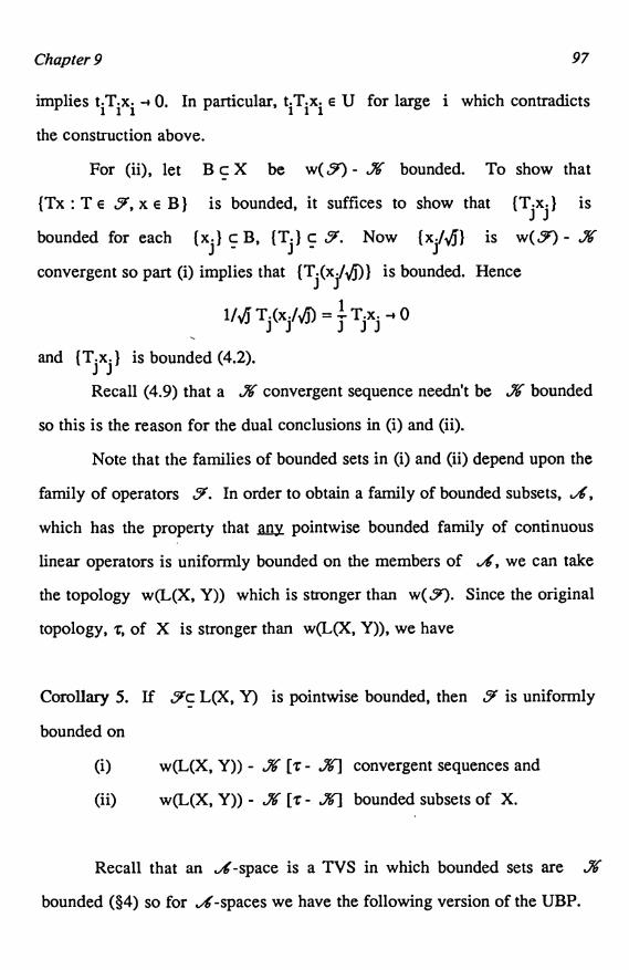
Chapter 9 97

implies tiTixi -4 0. In particular, tiT xi e U for large i which contradicts

the construction above.

For (ii), let B c X be w(5) - X bounded. To show that

(Tx : T E 91, x e B) is bounded, it suffices to show that (Tixi

) is

bounded for each (x{) c B, (Ti) c Y. Now { x(/ fj) is w(5) - X

convergent so part (i) implies that (T.(x./ ) is bounded. Hence

l/v J(./ J T.J -a 0

and { ) is bounded (4.2).

Recall (4.9) that a X convergent sequence needn't be ,% bounded

so this is the reason for the dual conclusions in (i) and (ii).

Note that the families of bounded sets in (i) and (ii) depend upon the

family of operators 51. In order to obtain a family of bounded subsets, ,4,

which has the property that my pointwise bounded family of continuous

linear operators is uniformly bounded on the members of A, we can take

the topology w(L(X, Y)) which is stronger than w(,9). Since the original

topology, ; of X is stronger than w(L(X, Y)), we have

Corollary 5. If Sc L(X, Y) is pointwise bounded, then 51 is uniformly

bounded on

(i) w(L(X, Y)) - X ['r - X] convergent sequences and

(ii) w(L(X, Y)) - X [ r - A] bounded subsets of X.

Recall that an 4-space is a TVS in which bounded sets are ,%

bounded (§4) so for IA-spaces we have the following version of the UBP.

Corollary 6. If X is an .A-space, then any pointwise bounded family

51c L(X, Y) is uniformly bounded on bounded subsets of X.

Without some form of completeness assumption, such as the

.A-space assumption in Corollary 6, the conclusion in Corollary 6 is false

(see Example 3). For semi-NLS, Corollary 6 takes the following form.

Corollary 7. Let X be a semi-NLS which is a Z-space and Y a

semi-NLS. If 51c L(X, Y) is pointwise bounded, then

(i) ( uITu1 : T E 5) is bounded and

(ii) 5 is equicontinuous.

Proof: (i) follows from Corollary 6 since 51 is uniformly bounded

on the unit ball {x E X : lixII <_ 1). (ii) follows from (i) and 5.21.

Example 3 shows that some sort of completeness-type assumption

on the domain space is necessary in Corollary 7.

Recall that a complete semi-NLS is a X-space (§2) so Corollary 7

is applicable to such spaces. This is the classical version of the UBP for

NLS. Mazur and Orlicz ([MO]) generalized conclusion (ii) of Corollary 7

to complete quasi-normed spaces. We can also obtain this form of the UBP

from Corollary 6.

Corollary 8. Let X be a quasi-normed X-space. If Sc L(X, Y) is

pointwise bounded, then 51 is equicontinuous.

Chapter 9 99

Proof: Let xi -4 0 in X and {Ti} c 5. Pick ti -+ - such that

tixi -40 (2.5). Then {tixi} is bounded so {Titixi} is bounded by

Corollary 6. Hence, I Titixi = Tixi - 0, and 9 is equicontinuous (5.20).i

Again recall that a complete quasi-normed space is a X-space (§2)

so Corollary 8 is applicable to such spaces.

In general, any equicontinuous family of continuous linear operators

is uniformly bounded on bounded sets (Exer. 2) so the conclusion in

Corollary 8 is sharper than that in Corollary 6. However, it is not generally

the case that a pointwise bounded family of continuous linear operators (or

even a family of operators which is uniformly bounded on bounded sets) is

equicontinuous as the following example shows.

Example 9. Let l2 have the topology w(12), where we consider each

element of l 2 to be a member of the dual of l 2 (Example 5.14). Then

{ek} is pointwise bounded on B 2 but is not equicontinuous with respect

to w(12) since ek - 0 in w($ 2) but <ek, ek> = 1 (5.20). As we will

see later (12, w(l2)) is an .A-space and the family {ek} is actually

uniformly bounded on bounded subsets of (12, w(t 2)) so the quasi-norm

assumption in Corollary 8 is important.

Despite this example which shows that a pointwise bounded family

of continuous linear operators needn't be equicontinuous, we will show later

in §25 that in the locally convex case there is always a stronger topology on

the domain space under which any pointwise bounded family of continuous


linear operators is equicontinuous.

A result which is closely related to the UBP is a result often referred

to as the Banach-Steinhaus Theorem. This result gives sufficient conditions

for the pointwise limit of a sequence of continuous linear operators to be

continuous. We first use the Basic Matrix Theorem to establish a general

form of this result.

Theorem 10. Suppose that (Ti) c L(X, Y) and lim Tix = Tx exists for

each x E X (we do not assume that T e L(X, Y)). Then lim Tix = T xi

converges uniformly for j E QI for each w((Ti)) - X convergence

sequence {x.} in X.

Proof: Consider the matrix M = [Tixj] in Y. From the definition

of w({Ti}) - X convergence, it follows immediately that M is a

Z-matrix so Theorem 2 gives the result.

Again the topology w({Ti}) depends upon the particular sequence

{Ti}, but if either of the stronger topologies, w(L(X, Y)) or the original

topology of X is used, then the same conclusion holds for these

topologies. In particular, we have

Corollary 11 (Banach-Steinhaus). Let X be a quasi-normed X-space and

{Ti} c L(X, Y). If lim Tix = Tx exists d x E X, then

(i) T is continuous, and

(ii) V compact subset K c X, lim Tix = Tx uniformly fori

Chapter 9 101

x E K.

Proof: (i): If J -40 in X, then { xi

) is X convergent so by

Theorem 10, lim Tixj = T x uniformly for j E IN. Therefore,i

imT =limlimTix. =limlimTixj =0.

(ii): From the sequential compactness of K, it suffices to show that

lim Ti = Tx uniformly for j E IN for any convergent sequence (x ) ini

X. But, if x -a x in X, then (xj - x) is X convergent in X so

lim Ti( - x) = T(x. - x) uniformly for j E IN by Theorem 10. Sincei

lim Tix = Tx, it follows that lim Tixi = T x uniformly for j r: IN.

i i-

The classical form of the Banach-Steinhaus Theorem assumes that

X is a complete quasi-normed space. Since any such space is a X-space,

Corollary 11 gives a generalization of the classical Banach-Steinhaus

Theorem to s-spaces.

Finally, we employ the UBP to obtain two interesting results which

will be employed later. First, we establish a simple and useful test for

determining the boundedness of a subset in a NLS.

Proposition 12. Let X be a semi-NLS. Then B c X is (norm) bounded if

and only if <x', B> is bounded d x' E X'.

Proof: =): clear.

t-: The family (Jb : b E B) is pointwise bounded on X' and X'

is complete (5.8) so the result is an immediate consequence of Corollary 7

and the fact that the canonical imbedding J is an isometry.

We will establish a more general form of this result later (14.15).

Finally, we give an application of the UBP to sequence spaces (see

also Exercises 4 and 5).

C*

Proposition 13. Let { ti } c R. Suppose that tisi converges V { si } E CO.

Then (t} E l 1

i=1

n

Proof: For each n define In : co -4R by <n' (s}> = tisii=1

00

Then n is linear, continuous and lim< n, (si}> = <f, (si}> _ siti

n i=1

exists d [si) E co. By Corollary 11, f is continuous so (ti) Ell since

c0 = l 1 (5.11).

Sargent Spaces:

Although the early versions of the UBP were established by using

sliding hump arguments, one of the most common methods currently used

to establish the UBP for NLS or QNLS is by use of the Baire Category

Theorem ([B]; see [Sw] for a historical description of the evolution of the

UBP). This method of proof was refined by W.L.C. Sargent and used to

Chapter 9 103

obtain an equicontinuous version of the UBP as in Corollary 8. We present

her results here.

Definition 14. A TVS X is called a Sargent space (a A3-space by Sargent)

([S]) if there exists no sequence of subsets (EkJ satisfying

(Si) 0 E Ek, Ek - Ek c Ek+1

00

(S2) X= u Ekk=1

(S3) Every Ek is nowhere dense.

A QNLS of second category (such a space is usually called a Baire

space) is obviously a Sargent space, but, remarkably, there are Sargent

spaces which are first category. See [S] for examples of such spaces.

For Sargent spaces we have the following UBP.

Theorem 15. Let X be a Sargent space, Y a semi-NLS and let

Y c (X, Y) be pointwise bounded on X. Then 9 is equicontinuous.

Proof: Let e > 0 and set

Ek = {xE X: IITxII <_2ke for all T E 5).

Then {E k} clearly satisfies (Si) and also satisfies (S2) since 9 ispointwise bounded. Hence, some Ek must be somewhere dense, i.e., there

exists x0 and a neighborhood of 0, U, such that x0 + U c Ek. If .X E U,

then x0 + x E Ek and x0 E Ek so by (S1) x = (x + x0) - x0 E Ek+l and

IITxII <_ 2k+le for all T E 9. Thus, W = (1/2k+1)U is a neighborhood of

0 with 11 Tx11 <_ a for all x e W and T e 9 so 5 is equicontinuous.

A more general form of the UBP for Sargent spaces is given in

Exer. 24.15.

Exercise 1. Let { ti.) c D and ij > 0. If lim t1. = 0 d j and lim ti. = 0i j

V i, show there is an increasing sequence of positive integers {p k) such

that I t 1:5e.. for i*j.ij

Exercise 2. If Sc L(X, Y) is equicontinuous, show that 9 is uniformly

bounded on bounded subsets of X.

Exercise 3. If X is a B-space and Y a semi-NLS and Tk E L(X, Y)

satisfies lim TO = Tx exists d x e X, show 1ITh 5 limjjTkjj < -.

Exercise 4. Establish the analogue of Proposition 13 with the space co

replaced by c and l p for 1 <_ p < °.

Exercise 5. Let (S, E, µ) be a a -finite measure space and 1:5 p < --

Suppose f : S -4 O is E-measurable and fg is µ-integrable d g e L"(U).

Show f E Lq(/.t), 1/p + 1/q = 1.

Exercise 6. Show Corollary 11 is false if the condition on X is dropped.00

[Hint: Consider f({ t))) _ t. on c00'jj=1

Chapter 9 105

9.1 Bilinear Maps

Let X, Y, Z be TVS. If f: X x Y -, Z, for x e X (y e Y) we

write f(x, ) (f(., y)) for the map f(x, )(y) = f(x, y) (f(-, y)(x) = f(x, y)).

A map B : X x Y -+ Z is ilin if B(x, ) (B( , y)) is linear d x E X

(V y e Y). We first establish the analogue of 5.1 for bilinear maps.

Proposition 1. A bilinear map B : X x Y -4Z is (jointly) continuous (with

respect to the product topology) if and only if B is continuous at (0, 0).

Proof: Let (x0, y0) E X x Y and W be a neighborhood of 0 in

Z. Choose a neighborhood of 0, W1, in Z such that

W1 + W1 + W1 c W. 3 balanced neighborhoods U1 of 0 in X and

V1 of 0 in Y such that B(U1, V1) c W1. Since U1 is absorbing,

3 t > 1 such that x0 E tUl and 3 s > 1 such that y0 E sV 1. Set

U = (1/s)U1, V = (1/t)V1.

If y e V, then B(x0, y) = B(x0/t, ty) E W1; if x e U, then

B(x, y0) = B(sx, y0/s) E W1. Thus, if (x, y) E U x V,

B(x0+x, y0+Y) - B(x0,Y0)

= B(x0,y) + B(X,y& + B(X,y) E W1 + W1 + Wl c W.

A map f: X x Y -+ Z is said to be separately continuous if f(x, )

and f(-, y) are continuous d x e X, y e Y. Even for bilinear maps

separate continuity does not imply joint continuity.


CO

Example 2. Define B : c00 X C00 -41R by B ({ sj } , ft)) _ sjtj (note this

j=1

is a finite sum). Note B is separately continuous but is not continuousk

[1/'/k J = xk -a 0 in c00 but B(xk, xk) = 1 V k].j=1

For X-convergent sequences we do have a form of sequential joint

continuity for separately continuous bilinear maps. Recall that w(L(Y, Z))

is the weakest topology on Y such that each element of L(Y, Z) is

continuous (§9).

Theorem 3. If xi -+ 0 in X and (yj ) is w(L(Y, Z)) - % convergent to

0 in Y and if B : X x Y -+ Z is a separately continuous bilinear map,

then lim B(xi, yj) = 0 uniformly for j E IN. In particular, lim B(xi, yi) = I-i

Proof: Since B(xk, y) -4 0 V y E Y, the sequence of linear operators

{B(xk, )} in L(Y, Z) is pointwise convergent to 0 on Y. The result

now follows from 9.10.

Since the original topology of Y is stronger than w(L(Y, Z)),

Theorem 3 also holds for the original topology of Y. As an immediate

consequence of Theorem 3, we obtain a classic of Mazur and Orlicz on

joint continuity.

Corollary 4 (Mazur-Orlicz). Let X and Y be QNLS with Y a X-space.

Chapter 9 107

If B : X x Y - Z is separately continuous and bilinear, then B is

continuous.

The first result of this type was established by Mazur and Orlicz

when Y is a complete QNLS ([MO]). Corollary 4 gives a generalization

of their result to X-spaces.

Using Corollary 4 we can weaken axiom (v) in Definition 2.1 of a

quasi-normed space. If we assume that scalar multiplication is only

separately continuous (with respect to the metric topology induced by the

function ), then it follows that scalar multiplication is actually

continuous since the scalar field is complete.

Bourbaki introduced a concept, called hypocontinuity, for bilinear

maps which is intermediate between separate continuity and continuity.

Definition 5. Let B : X x Y -4 Z be bilinear and separately continuous,

and let Y be a family of bounded subsets of Y. B is 7L-hypocontinuous

if for every neighborhood of 0, W, in Z and every A E Jl, 3 a

neighborhood of 0, U, in X such that B(U, A) c W.

Thus, B is y-hypocontinuous if and only if whenever [x3) is a

net which converges to 0 in X and A E JI, lim B(xb, y) = 0 uniformly

for y E A. If X is metrizable, the same statement holds with sequences

replacing nets.

If ,fix (2y) is the family of all bounded subsets of X (Y) and B

is both ,fix and 2 y hypocontinuous, then B is said to be

hypocontinuous.


Example 1 shows that a separately continuous bilinear map needn'tk k

be hypocontinuous [if xk = ej/k and A = (yk = I e j : k e a), thenj=1 j=1

Xk -4 0 but B(xk, yk) = 1]. However, we show that any separately

continuous bilinear map is hypocontinuous with respect to the family of X

bounded sets.

Theorem 6. Let X be a QNLS and B : X x Y -4Z bilinear, separately

continuous. Then B is Xy hypocontinuous, where Xy is the family of

w(L(Y, Z)) - .% bounded subsets of Y.

Proof: It suffices to show that B(xk, yk) - 0 whenever xk -4 0 in

X and (yk) is w(L(Y, Z)) - X bounded. Pick tk - co such that

tkxk -a 0 (2.5). Then {yk/tk} is w(L(Y, Z)) - X convergent to 0 so

B(xk, yk) = B(tkxk, yk/tk) -40 by Theorem 3.

The conclusion of Theorem 6 is also valid for the family of subsets

of Y which are 96 bounded with respect to the original topology of Y.

Any continuous bilinear map is hypocontinuous (Exer. 1), but there

are hypocontinuous bilinear maps which are not continuous. Examples of

such bilinear mappings are given in 23.15, 23.16.

We consider results analogous to Theorem 3 and Corollary 4 for

families of bilinear mappings. Let 51 be a family of separately continuous

bilinear mappings from X x Y into Z. The family 5 is 1cft (righx)

equicontinuous if d y E Y (V x e X), the family 9!y = (B(-, y) : B E 51)

((B(x, ) : B E 5r)) is equicontinuous in L(X, Z) (L(Y, Z)). The

Chapter 9 109

sequence in Example 9 below shows that a family can be left

equicontinuous but not right equicontinuous. The family S is

equicontinuous if it is equicontinuous as a family of mappings from X x Y

into Z. As in Proposition 1, 51 is equicontinuous if and only if S is

equicontinuous at (0, 0) (Exer. 4). Analogous to Theorem 3 we have

Theorem 7. Let 9 be left equicontinuous. If xi -40 in X and (yi) is

X convergent in Y, then lim B(xi, yi) = 0 uniformly for B e Y.

Proof: It suffices to show that lim Bi(xi, yd = 0 for each

(Bi) c 51. Consider the matrix M = [Bi(xi, yi)]. Since S is leftequicontinuous, the columns of M converge to 0. For any increasing

sequence of positive integers (m ), there is a subsequence of (rr . )00

such that the series Gyn converges to a point y E Y. Thenj =lJ

cc

I Bi(xi, yn) = Bi(xi, y) -+ 0 by the separate continuity and the leftj=l . J

equicontinuity of Y. Thus, M is a X-matrix and by the Basic Matrix

Theorem lim Bi(xi, yi) = 0.

We have the immediate corollary analogous to Corollary 4.

Corollary 8. If X and Y are QNLS with Y a X-space, then any left

equicontinuous family of bilinear maps is equicontinuous.


Without some type of completeness assumption, Corollary 8 is false.

Example 9. For each i E IN define Bi x c00 - IR by

Bi((s.), (t-}) _ sj-tj.

j=1

Each Bi is separately continuous and the sequence (Bi) is left

equicontinuous [if (t1, ..., tn, 0, ...) E c00, then for i >_ n

n

Bi({ }, (t{}) = siti]. However, (Bi} is not even right equicontinuous;

j=1i

for if e = (1, 1, ...) E I'* and yi = ejl, then Bi(e, yi) = 1 while

j=1

yi-.0.

From Corollary 8 we obtain an analogue of Corollary 9.7 for

bilinear maps.

Corollary 10. Let X, Y be QNLS which are X-spaces. If 9 is a family

of separately continuous bilinear maps which is pointwise bounded on

X X Y, then 5 is equicontinuous.

Proof: For y E Y the family (B(-, y) : B E 5) c L(X, Z) is

pointwise bounded on X and, therefore, equicontinuous by 9.7. That is, 3

is left equicontinuous. The result follows from Corollary 8.

Chapter 9 111

Corollary 10 gives a generalization of Theorem 15.12 of [Gr]; see

also 14(3) of [K1]. The proofs in these references use the theory of

uniform spaces while the proof above uses only basic properties of

convergent sequences and the Basic Matrix Theorem.

Exercise 1. Show any continuous bilinear map is hypocontinuous.

Exercise 2. Show a bilinear map B : X x Y -4 Z between semi-NLS X, Y

and Z is continuous if and only if sup( IIB(x, y)II : IIxil s 1, IIYII <_ 1) < o.

(Compare with 5.5.)

Exercise 3. Let .4 be a family of bounded subsets of X. Show a

separately continuous bilinear map B : X x Y -4Z is -hypocontinuous if

and only if V A E .4 the family (B(x, ) : x E A) c L(Y, Z) is

equicontinuous.

Exercise 4. Show that a family of bilinear maps is equicontinuous if and

only if it is equicontinuous at (0, 0).

Exercise 5. Show that if 9 is left equicontinuous, then 9 is pointwise

bounded on X x Y. Thus, the converse of Corollary 10 holds.

Exercise 6. Show that if 9 is equicontinuous, then 5 is uniformly

bounded on sets of the form C x D, where C is bounded in X and D is

bounded in Y. (Compare with Exer. 9.2.)


9.2 The Nikodym Boundedness Theorem

The Nikodym Boundedness Theorem is a "striking improvement" in

the UBP for the space of countably additive measures defined on a

a -algebra ([DS] IV.9.8 ). The theorem has been extended to the case of

bounded finitely additive measures and we consider this more general

version. We begin by establishing a remarkable lemma of Drewnowski

([Dr]) which shows that in some sense a bounded finitely additive set

function is "not too far" from being countably additive.

Let E be a a-algebra of subsets of a set S. Recall that ba(s) is

Rthe B-space of all bounded, finitely additive set functions p : Z A

equipped with the variation norm, 11µd = J u I (S) (2.30). If p E ba(s) and

(E ) is a pairwise disjoint sequence from E, thenn n

IA(E-)I s IAI(.vlE)E-):5 IAI(S) b nJ

j=1

so the series I p(EE) is absolutely convergent. Thus, if a finitely additivej=1

set function, p e ba(s), fails to be countably additive, it is not because theCO

series p(EE) fails to converge but rather that it fails to converge to thej=1

CO

"proper" value, p( v E.).j=1 J

Lemma 1 (Drewnowski [Dr]). Let p e ba(s). If (E } is a pairwise

disjoint sequence from s, then 3 a subsequence (En) such that p isJ

countably additive on the a -algebra generated by { En) .

J

Chapter 9 113

Proof: Partition IN into a pairwise disjoint sequence of infinite sets

{0} By the observation above, ( u E) -+ 0 as i --4 -. So 3 ijeKi

such that u I ( u E) < 1/2. Let N1 = Ki and nl = inf N1. NowjeKi

partition N1\(nl) into a pairwise disjoint sequence of infinite sets

(0}*1. As before 3 i such that Ju I ( u E.) < 1/22. Let N2 = K2

jEK2

and n2 = inf N2. Note n2 > n 1 and N2 c N1. Continuing produces a

subsequence n}T- and a sequence of infinite subsets of IN, (Ni), such that

j+l c N and (u Ei) < 1/2J. Let EO be the a-algebra generatediE N.

J

by {EnJ}.

We claim that µ is countably additive on EO. If {Hk} c E0 and

Hk j0, then I ! (Hk) 5 i I (Hk)10 so u is countably additive [given j,

3 Hi such that--mm n Hi > nj so lgl(Hi):5 Jµ J( u En ) < 1/2J].k?j k

Corollary 2 (Drewnowski). Let µi E ba(E) for i E IN. If (E } is a

pairwise disjoint sequence from E, 3 a subsequence {En } such that eachj

µi is countably additive on the a-algebra generated by {En }.J

luiI(E)Proof: Set µ(E) =

1 I

w 21 + µl Then µ e ba(E) (2.30, 2.9)M

so by Lemma 1, 3 a subsequence (En) such that µ is countably


additive on the a -algebra, E0, generated by (En ). If (H) c EO andJ

H-10, then lim pi(H.) = 0 for each i, and pi is countably additive on1

Y-0-

Finally, we require the following technical lemma.

Lemma 3. Let f be an algebra of subsets of set S, and let pi : 4 -+ R

be bounded and finitely additive for i e N. Then [pi(A) : i E IN, A E .A)

is bounded if and only if [pi(A) : i, j E a) is bounded for each pairwise

disjoint sequence (Ai

) from 4.

Proof: Suppose sup( I pi(A) : i E IN, A E if) = -. Note that for

each M > 0 3 a partition (E, F) of S and an integer i such that

min pi(E) pi(F) I ) > M. [This follows since

Ipi(E) I > M + sup( Ipi(S) I : i e IN)

implies I pi(S\E) I >_ I pi(E) - 1pi(S) I > M.] Hence, 3 it and a partition

(El, F1) of S such that min(Ipi1(E1)J, Ipi1(F)I ) > 1. Now either

sup( lpi(HnEl)I : H E A IN) = - or

sup( lpi(HnFl) :HE 4,iEIN)

Pick whichever of E 1 or F1 satisfies this condition and label it B 1 and

set A1

= S\BI*

Now treat B l as S above to obtain a partition (A2, B2)

of B 1 and an i2 > i l satisfying I pi (A2) 1 > 2 and2

, i E a } = oo .sup( I pi(H n B2) 1 :HE

Proceeding produces a subsequence (ii) and a disjoint sequence (A )

Chapter 9 115

such that 1µi (A) > j. This establishes the sufficiency; the necessity isJ

clear.

We now establish the Nikodym Boundedness Theorem for bounded,

finitely additive set functions.

Theorem 4. Let {µi} c ba(E). If {µi) is pointwise bounded on E, then

(pi(E) : i E Qi, E E E) is bounded, i.e., {µi) is uniformly bounded on E.

Proof: By Lemma 3 it suffices to show that (Ni(E.) : i, j E IN) is

bounded for each pairwise disjoint sequence (E) from E.

Let c(E) be the space of Z-simple, real-valued functions equipped

with the sup-norm (2.31). The dual of eY(E) is ba(E) (5.15 and Exer.

5.3) so each µi induces a continuous linear function on cY(E) via

integration, <µi, tp> = fS tp dµi, and I JµiI I = 1µi (S). Consider the

sequence {CE } in eY(E). By Corollary 2, any subsequence of {E } has

a subsequence (En ) such that each µi is countably additive on theJ

algebra generated by {En }. This means that (CE) isJ J

coCO

w((ui)) - X

convergent in eY(E) [ µi(En) = ii(u En) V i]. The hypothesis of thej=1 J J=1 J

theorem implies that the sequence (µi) is pointwise bounded on QY(E)

so the General UBP 9.4(i) yields that (µ.(E) : i, j) is bounded and the

proof is complete.

Note that the space e(l) is not complete (in general, it is not even

second category [Sa]) so the classical form of the UBP is not applicable.

Also note that the sequence (CE ) above is not norm - ,convergent soJ

9.7 is not applicable; the general form of the UBP given in 9.4 seems to be

necessary.

From the inequality µ I (S) S 2 sup (lµ(E) 1: E E E) (Example

2.30), it follows that the norms of the linear functionals, (1111iII ), in

Theorem 4 are bounded. If the conclusion is written in this form, the

theorem has the flavor of the classical UBP for B-spaces (9.7).

If E is the a-algebra of all subsets of IN, then eY(E) is just the

space m0 of Example 2.18 which has for its dual ba (Exer. 5.3 and

Example 5.15). For later use, we give a statement of this special case.

Corollary 5. If (µi) c ba is pointwise bounded on m0, then (11µill) is

bounded.

We can now obtain an analogue of Proposition 9.13 for m0.

cc

Proposition 6. If (ri ) E IR is such that riti converges V(ti) E m0, theni=1

Ca

<R, (ti )> _riti defines a continuous linear functional on m0 with

i=100

IIRII = I ri I < °°

i=1

Chapter 9 117

n

Proof: For each n define Rn : m0 -s UZ by <Rn' (t')>j=1

n

Then Rn is continuous on m0 with IIRnII = I1. Since

j=1

<Rn, {J

}> -4<R, {J

}>,

it follows from Corollary 5 that R is continuous andHE

IIRII - limIIRnII = I j I <j=1

n

(see Exer. 9.3). For each n, set xn = (sign r.)ej. Thenj=1

n

IIRII >- <R, xn> _ I I so IIRII ? Irj1.j=1 j=1

IIxnII=1 and

The Nikodym Boundedness Theorem is such a striking result that it

has been generalized in many different directions (see, however, Exer. 1).

For example, the a -algebra assumption has been relaxed and the range of

the measures has been replaced by TVS's. For the history of the evolution

of these generalizations and references, see [DU}.

Exercise 1. Let ,4 be the family of all subsets of IN which are either

finite or have finite complements. Let n : X -4 1 be given by S(E) = 1

if n E E and Sn(E) = 0 otherwise. Define

An(E) = n(n+l(E) - Sn(E)) if E is finite and

Nn(E) _ -n(n+1(E) - n(E))

µn : X - UZ by

otherwise. Show that f is an algebra, (µn} is pointwise bounded on .4

but is not uniformly bounded on A. Thus, the o-algebra assumption in

Theorem 4 cannot be replaced with E being an algebra.

Exercise 2. Let X be a NLS and E a a -algebra. Let µn : E -4X be

finitely additive and have bounded range d n e W. If (µn(E)) is bounded

V E E E, show sup( Ilµn(E)II : n e al, E E E) < oo.

Chapter 9 119

9.3 Fourier Series

Given a periodic function f : U -+ U of period 27c belonging to2n

L1 [0, 27r], its Fourier coefficients are given by cn(f) = n I f(t)e intdt0

and the nth partial sum of the Fourier series for f is

27rn

=f(s) 1 L

eij(t-s)ds=j 2

f(s)Dn(t - s)ds,J0 J0j=-n j=-n

where Dn(t) = skin+t/2)t is the Dirichlet kernel ([HS] 18.27).

One of the problems of Fourier analysis is to determine the

convergence of the Fourier series of a function f. We show that the UBP

can be used to show the existence of a continuous periodic function whose

Fourier series diverges at 0. For this, the following lemma is useful.

Lemma 1. Let g : [a, b] - D be continuous. Define G : C[a, b] -4 U by

b bG(f) = Ja g(t)f(t)dt. Then G is linear and continuous with IIGII = I I g

a

bProof: Since I G(f) I <_ IIf IIJ I g I, G is linear, continuous and

ab

IIGII <_ J I g I Fix n E IN. Thena

+n gIJbIgI = JbI I 1+n g

_ fb

+ngga a a

+ Jg 1+ngg J+ G(+n g )

a a

5bna

+ IIGII11

+n g IL s bna + IIGII

fbso

JIgl<_IIGII

a

Now let fn : C[0, 27r] -4R be defined by

2nn(q) = 1f0 q,(s)Dn(s)ds,

i.e., n(T) is the nth partial sum of the Fourier series of (p evaluated at

2nt = 0. By Lemma 1, II nII = T Ji Dc(s) I ds. We claim that

0j2,

I Dn(s) I ds) is unbounded. Since sin u S u for 0 <_ u 5 ir, this will0

jfollowif ( I

sin(un+1)uI du } is unbounded. But,

O

2n

JrI sin(2n+1)u I du = f

2n+1Isin(2n+l)u I du

0 k-01

2n (k+1)7r

2n+1 2n+1> 1 1 I sin(2n+1)u I du

k=0 J kzc2n+1

2n (k+1)nI CJ Isin vIdvk=0

k?r

2n_2 e 1

r L k+I -k=O

It now follows from Corollary 9.7 that there must exist a continuous,

periodic function 9 whose Fourier series diverges at 0 because otherwise

the sequence (Ilnil ) would be bounded. Of course, the same argument

applies to any point in [0, 27r].

We can use a construction of Banach and Steinhaus, called

(k+1)7r

Chapter 9 121

condensation of singularities, to show the existence of a continuous,

periodic function whose Fourier series diverges at a sequence of points in

[0, 2ir].

Theorem 2 (Banach, Steinhaus). Let X be a B-space, Yk a NLS and

Tk E L(X, Yk) V k E IN. Then B = (x E X : limliTkxll < co) either

coincides with X or is first category in X.

Proof: Suppose B is second category in X. By the definition of

1C*

B, d x e B lira supllk Tnxll = 0. Let ->O. Then B c v Bk, wherek n>_1 k=1

Bk = (x E X : supllk Tnxll <_ E). Each Bk is closed so some Bk containsn>_1

a sphere, i.e., 3x0 E X n Bk, r> 0 such that

lix-x011 <_r* supllkTnxll SE.

Thus, for lizll <_ r, if x = x0 + z, then Ilk TnzII Ilk TnxII + Ilk Tnx0ll <_ 2e

and suplITnzll <_ 2Ek. Hence, X = B since B is a linear subspace.n

Corollary 3 (Condensation of Singularities). Let Tp,q, p, q E IN, be a

sequence of continuous linear operators from a B-space X into a NLS Yq

Suppose d p 3 xp E X such that TTmlITp,gxpll = . Thenq

B=(xEX:ri-mIITp,gxli=OOVpEIN)q

is second category in X.

Proof: V p Bp = (x E X : l 11Tp,gxjj < -) is first category in Xq

00

by Theorem 2 and the hypothesis. Thus, B = X\ u B is second category.p=1 p

Now let { sj } be a sequence of distinct points from [0, 2n]. Let

Snj ((p) be the nth partial sum of the Fourier series of the continuous

periodic function qp evaluated at sj. By the example above d j 3Tj

such

that n I By Corollary 3, 3 T such that

nr' mV j, i.e., 3 a continuous, periodic function ip whose Fourier series diverges

at each ti. Actually, Rudin shows that the set of divergent points is a dense

GS set, and then shows by a simple argument that in a complete metric

space every dense GS set is uncountable ([Rul]).

Chapter 9 123

9.4 Vector-Valued Analytic Functions

In order to extend a property of scalar-valued functions to a function

with values in a Banach space there are often two natural approaches. One

is to simply replace the absolute values in the scalar field by norms; this

leads to what is generally referred to as a strong property. The second

approach is to compose the Banach space valued function with an arbitrary

continuous linear functional from the dual of the Banach space and require

the resulting scalar-valued function to have the property being considered;

this leads to what is called a weak property. We now consider such a

situation for analytic functions; we will later consider integration of

vector-valued functions.

Let D be an open subset of the complex plane. Let X be acomplex B-space and f : D -, X. If z0 E D, we say that f is differentiable

f(z)- f (z0)at z0 with derivative f' (z0) provided the limit 1 i m z-z = f' (z0)

z-4z0 0

exists with respect to the norm topology. We say that f is (strongly)

analytic on D if f is differentiable at every point in D. We say that f is

weakly analytic on D if the function x' f : D -4 C is analytic on D

V X' E X'. We now show that, surprisingly, these two notions of

analyticity coincide.

Theorem 1 (Dunford). If f : D - X is weakly analytic on D, then f isanalytic on D.

Proof: Let z0 E D. Since X is complete, it suffices to show that

f(z)- f (z0) f(w) - f (zd

z)-

w)-- 0 as z, w - z0. Let C be a positively oriented

0 0

circle with center at z0 and radius r such that C and its interior lies

inside D. For x' a X', x'f is continuous on C so the UBP implies that

3 M > 0 such that 11f(z)11:5 M d z E C. For x' E X', we have

1 f x'f(z)X' f(z0) _ J dzCz - z0

by Cauchy's Integral Formula. If 0 _ r/2, IX-wl >_ r/2 for )L E C. By 8.1.5

f(z)- f(z& f(w)- f(z0)4M z-w11 -- II

S ,z-z0 w-z0 rand the result follows.

For a history of vector-valued analytic functions, see [Ta].

Exercise 1. Define Riemann integrability for a function f : [a, b] - X with

values in a B-space.

Exercise 2. Prove a vector version of Liouville's Theorem. That is, if

f : C - X is analytic and bounded, then f is a constant.

Chapter 9 125

9.5 Summability

A summability method for sequences is an attempt to attach a notion

of convergence to certain divergent sequences. For example, the classical

Cesaro summability method takes a sequence (tk) and associates with itk

the sequence of averages sk = t./k. If the original sequence (tk}

j=1

converges to t, then also sk -4 t. However, there are divergent sequences

{tk} such that the sequence (sk) converges; for example, take tk = (-1)k

The Cesaro method of summability can be described by employing infinite

matrices.

Let A = [abe an infinite matrix of real numbers: If X and Y

are vector spaces of real-valued sequences, we say that the matrix A

belongs to the class (X, Y) if for each x = (x j } e X, the sequence

aij -) 1=1= Ax

j=1

belongs to Y (note this requires that the series a..x. converges for

j=1

each i). Thus, to say that a matrix belongs to the class (c, c) means that

it transforms convergent sequences into convergent sequences. A matrix of

class (c, c) is said to be regular if it preserves limits, i.e., if

lim xi = lim aijJ for each x e c. Cesaro summability can be describedj=1

in this manner by using the matrix

1 0 0 .....1/2 1/2 0 .....

A= 1/3 1/3 1/3 0 .. ,

and from the convergence properties discussed above, this matrix is regular.

We use the results on the UBP to establish several classic results in

summability theory. We first require several preliminary observations.

Lemma 1. Let . E IR, j E IN. If 3 M > 0 such that I t. 1 5 M for everyjEa

00

finite set a c IN, then I tj 1 S 2M.

j=1

Proof: For a c IN finite, let a+ _ (k E a : tk ? 0),

a = (k E a : tk < 0). Then 1tk1 _ tk 5 M andkE a+ kE a+

Itk1 _- tkSMkE a kE a

00

so Itk i :52M. Since a is arbitrary, I tk :52M.kE a k=1

The complex case of Lemma 1 is given in Exercise 1.CO

Lemma 2. Assume that I aij I < 00 V i and lim aij = exists d j. Letij=1

(a c (N: a finite). If lim aij = aj is not uniform for a e 51,i jEa jEa

Chapter 9 127

then 3 e> 0, an increasing sequence, (ij), of positive integers and a

pairwise disjoint sequence {

J} c Y such that I

kE

IiJ

(ai k - ak) >_ e d j.

. J

Proof: Suppose the limit is not uniform for 6 e 9. Then 3 e > 0

such that d i'3 k. > i and a finite set c such that I (ak k - ak) 2e.

kE 61

Put i 1 = 1 and let a 1 E9 be such that I (ai k - ak) 2a

kE 61

M1

Set rl = 61 and M1 = max a1. 3 n1 such that laij - J <e for

i?n1. 3i2>max{i1,n1} and 62E 9such that

Set r2 = 62\61 and note

j=1CG (ai k - ak) 12 2e.

kE 62

I (ai2k - ak) I >_I

(ai2k - ak) I - k I ai2k - akI >_ 2e - e = e.

kE z2 kE 62 kE 61

Continuing by induction produces the desired sequences.

We now establish a result which contains two summability results of

Hahn and Schur. Recall that m0 is the subspace of l °° which consists of

the sequences with finite range.

Theorem 3. For a real infinite matrix A = [aij], the following are

equivalent.

(i) A E (l °°, c),

128

(III) lim I aiji

j=1

(ii) A E (m0, C),

(iii) (I) lim ai

= aj exists d j

(II) { aij } and { ai } belong to l 1 V i

CO

(iv) (I) and

The Uniform Boundedness Principle (UBP)

aI =0.

(IV) ( aij I j E l 1 d i and I I aij I converges uniformly for

J

Proof: Clearly (i) implies (ii). Suppose (ii) holds. Then (I) follows

by setting x = ej E m0. Each row (aij ) j induces a continuous linearco

functional Ri on m0 defined by <Ri, x> = ) aij j, x = (xj ) E m0, with

j=100

RiII = I I aij 1 (9.2.6). We claim that lim I aij = ) uniformly for

j=1 1 jE6 jE6

a E 9, the finite subsets of M. For assume that this is not the case and let

the notation be as in Lemma 2. The sequence (C'C

) is w(l 1) - J6J

convergent in m0 so in particular it is w((Ri)) - X convergent. Since

lim Ri(x) = R(x) exists d x E m0, the general Banach-Steinhaus Theorem

(9.10) implies that

lim Ri(C.r) = lim I aik = R(Cz) _ ak1

J 1 kEZj J kEZj

converges uniformly for j e IN. But, this contradicts the conclusion of

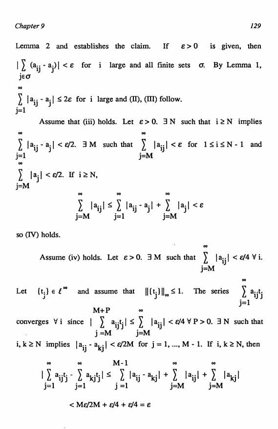
Chapter 9 129

Lemma 2 and establishes the claim. If e > 0 is given, then

(aij - aj) I < e for i large and all finite sets a. By Lemma 1,jEa00

I I aij - aj I <_ 2e for i large and (U), (III) follow.j=1

Assume that (iii) holds. Let e > 0. 3 N such that i N impliesco 00

aij - . ( <&(2. 3M such that I Jaij j <e for 1 S i <_ N - 1 and

j=1 j=M00

IajI <E/2. If izN,j=M

00 W CO

IaijI <_ I aij - aj I + aj I <ej=M j=1 j=M

so (IV) holds.W

Assume (iv) holds. Let e > 0. 3 M such that I I aij I < e/4 V i.

j=MCO

Let { ti) E l °° and assume that 11(t) II. < 1. The series aijtj

j=1M+P co

converges V i since I aij 1<_ I aij I < e/4 V P > 0. 3 N such that

j =M j=Mi, k z N implies I aij - akj I < c/2M for j = 1, ..., M - 1. If i, k N, then

00 00 M-1 00 00

G aijt - akjtl <_ Iaij - akjI + IaijI + I I akjj=1 j=1 j =1 j=M j=M

<Mc/2M+F/4+F/4=e


00

so lim aijJ exists and (i) holds.

i j=1

The equivalence of (i) and (iv) is a classic result of summability due

to Schur ([Sc]). Schur's result was generalized by Hahn who established

the equivalence of (i) and (ii) ([Ha]). It is interesting that Hahn obtained

his result as a consequence of an abstract UBP, one of the earliest abstract

forms of the UBP. We will use this result later in § 16 to give an interesting

example of weak convergence in l 1

In 9.2 we established a result of Nikodym on the boundedness of

families of measures. There is another result of Nikodym, called the

Nikodym Convergence Theorem, on measures which is an immediate

consequence of Theorem 3. Let E be a a-algebra of subsets of a set S,

and let pi : E -' Ut be a sequence of countably additive set functions on E.

The sequence {pi} is said to be uniformly countably additive if for every

pairwise disjoint sequence

00

(E } from E, the series pi(E) are

j=1

uniformly convergent for i e IN.

Theorem 4 (Nikodym Convergence Theorem). If lim pi(E) = p(E) exists

for each E E E, then (pi) is uniformly countably additive and p is

countably additive.

Proof: Let (E ) be a pairwise disjoint sequence from L. Set

aij = pi(E) and A = [aij]. Then A E (m0, c) by hypothesis so the

Chapter 9 131

conclusion follows from Theorem 3.

The Nikodym Convergence Theorem has generalizations to finitely

additive, vector-valued set functions. For a discussion of these

generalizations and the historical development of the theorem, see [DU].

We use the UBP to establish another result of summability theory

due to Silvermann and Toeplitz. This result gives necessary and sufficient

conditions for a matrix A to belong to the class (c, c) and to be regular.

Theorem S. The matrix A belongs to (c, c) and is regular if and only if00

(i) sup I Jaij j< -,i j=l

(ii) lim aij = 0 for each j e IN, andi

00

(iii) lim aij = 1.

i j=1

Proof: If A e (c, c) is regular, then (ii) and (iii) follow by setting

x = e and x = (1, 1, ...). For (i) note that each row (aij) J =1 induces a00

continuous linear functional Ri on

with norm

00

c by Rix = I aij xi, X= (x

i) a c,

j=1

aij I (Exer. 9.4). Since A E (c, c), lim Ri(x) exists

j=l i

IIRiII =

00

V x E c so by the UBP (9.7) suplIR111 = sip I aij I < 00 and (i) holds.

j=1

Co

Suppose that (i), (ii) and (iii) hold. Then (i) implies that I aij

j=1converges d {J } E c. Let x = (xj) e c with l =lim xj. Let e> 0. Set

CO

M = max { sup I aij I, sup lJ - Choose N such that lJ - l I < Ei j=1

for j >_ N. WriteCO N

(1) I aij x-el <_ 1 laijlIx -tlj=1 j=1

Co

+ : laijIIij=N+1

Do

-LI+1LlI1 aij-11.j=1

The second term on the right hand side of (1) is less than Me by (i). With

N fixed by (ii) the first term is less than M- NE for i large and the last

term is less than l E for i large by (iii). Thus, Ax e c and

lim Ax = 1.

The sufficiency of (i), (ii) and (iii) is due to Silvermann; the

necessity is due to Toeplitz.

Another interesting result of summability related to the Silvermann-

Toeplitz Theorem is a theorem due to Steinhaus which asserts that a regular

matrix A belonging to the class (c, c) cannot "sum" all bounded

sequences, i.e., cannot belong to the class (l c). A more general form of

this theorem asserts that a regular matrix A E (c, c) cannot belong to

(m0, c), i.e., cannot "sum" all sequences of 0's and l's. We can give a

simple proof of Steinhaus' Theorem based on Theorem 3.

Chapter 9 133

Theorem 6 (Steinhaus). If A E (c, c) is regular, then A ¢ (m0, c).

Proof: Suppose that A = [aij] E (m0, c). By Theorem 3,

lim aij = a. exists for each j, {aj} E l 1 andi

00 0*

lim I aijl = R((x(}) _ a(xj

i j=1 j=1

for each (i ) E m0. For each n let xn be the sequence with 0 in the

first n coordinates and 1 in the other coordinates. Then Rxn = 1 for00

each n since A is regular while Rxn = aj -+ 0. This contradiction

j=n+1

establishes the result.

Finally, we use the UBP 9.7 to establish an interesting result of

Hellinger and Toeplitz on matrices which map e 2 into itself. Hellinger

and Toeplitz showed that if

(2) GyiGaij J converges d x = (xi ), y = (yi ) E l 2 ,

i j

then there is a constant M such that

(3) 1 GyiGaij j I s M for 11X112,11Y112 s 1 ([ T]).

i j

If (2) holds d y E l 2, then AXE l 2 b x E l 2 (Exer. 9.4), i.e.,

1,A E (L 2I 2), and (3) implies that IIAxII2 < _ M V X E l 2 with 1142:5

i.e., A : l 2 - Q 2 is a continuous linear operator. We use 9.7 to give a

simple proof of this result.

Theorem 7. If A E (12, 12), then A : 12 -41 2 is continuous.

Proof: If x, y E 12, we write x y = Lxiyi. Let ai be the ith rowi

of the matrix A = [asince A E (12, l2), each ai E l2 (Exer. 9.4).n

Define An : 12.412 by Anx= (ai x)ei. Then each An is linear and

i=1

continuous and lim y Anx = y Ax for each x, y e 12. Thus, (Anx : n)

is norm bounded in 12 V x (9.12), and by the UBP 9.7, (IjAn1l) is

bounded, say, by M. Since I y Anx 1 5 M for IIx112, 11y112112:5 1. and

y Anx -4y-Ax, (3) follows.

Exercise 1. If tk e C and I I tk1 5 M for every finite a, showkEa

00

tk ( 5 4M.

k=1

CO

Exercise 2. Show A = [aij] E (CO, 10') if and only if (a) sup I ( aij I < 00

i j=1

Exercise 3. Show A = [aij] E (CO, c) if and only if (a) and (flim aij = aj exists V j.i

Exercise 4. Show A= [aij] E (c0, co) if and only if (a), (j3) and aj = 0

dj.

Chapter 9 135

00

Exercise 5. Show A E (c, c) if and only if (a) and d p limail

= api

l=pexists.

Exercise 6. Check conditions (i), (ii), (iii) of Theorem 5 for the Cesaro

matrix.

10

The Open Mapping and ClosedGraph Theorems

In this section we establish two important results of Banach, the

Open Mapping and Closed Graph Theorems ([B]).

Let X and Y be quasi-normed spaces.

Lemma 1. Let T E L(X, Y) be such that AT is second category in Y.

If U is a neighborhood of 0 in X, then TU contains a neighborhood of

0 [mappings with this property are called almost openl.

Proof: Let V be a balanced neighborhood of 0 in X such that

V + V C U. Now X = u kV so TX = u kTV. By the second categoryk=1 k=1

assumption some kTV = k(TV) contains an open set W. Therefore,

TUoTV - TV:) TV - TV: j(W - W) and j(W - W) is an open

neighborhood of 0 in Y.

137

138 The Open Mapping and Closed Graph Theorems

Lemma 2. Let X be complete. If T E L(X, Y) is almost open, then T

is open (and, hence, onto).

Proof: Let S(r) = (x e X : I x I < r). Since every neighborhood of

0 in X contains some S(r), it suffices to show that T(S(r)) is a

neighborhood of 0 for each r > 0. For n = 0, 1, 2, ..., let Gn = S(r/2).

By hypothesis, TGn is a neighborhood of 0 in Y so 3 e > 0 such that

(1) TG nJHn={yEY: jyj <En},

and we may assume that n - 0.

Then H 1 c TGO; for if y E H 1, then by (1) 3 x l E G 1 such that

y - Tx1 I < e2 or y - Tx1 E H2. By (1) 3 x2 E G2 such that

y - Tx1 - Tx2 1 < e3 or y - Tx1 - Tx2 E H3. By induction, 3 xn E Gn

such that I y - Tx 1 - Tx2 - ... - Txn i

00

< -n+1' Thus, y = Txk and sincek=1

00

I xk I < r/2k, the series xk converges to some x E X. Sincek=1

00 00

lxi <_ lxki < r/2k=r,k=1 k=1

x e GO and continuity implies that Tx = y e TGO so H1 c TGO. Thus,

TGO is a neighborhood of 0.

Theorem 3 (Open Mapping Theorem, OMT). Let X be complete. If

T E L(X, Y) is such that AT is second category in Y, then T is open

Chapter 10 139

(and, hence, onto).

Proof: Lemmas 1 and 2.

Theorem 3 holds in particular if both X and Y are complete and

T is onto, but there are examples of NLS which are second category but

not complete ([Bo] Exer. III.4.4).

Corollary 4. If X and Y are complete and T E L(X, Y) is 1-1 and onto,

then T is a homeomorphism.

Corollary 5. Suppose the vector space X is a quasi-normed space under

the two complete quasi-norms I 1 and 2. If I 1 is stronger than

12' thenI I 1

and1

12 are equivalent.

Proof: The identity map from (X,1)

to (X, 2) is

continuous so Corollary 4 gives the result.

Example 6. The completeness of both quasi-norms in Corollary 5 is

important. The identity map I : (C[0, 1], 1111) - (C[0, 1], 11111) is

continuous but does not have a continuous inverse. This example also

shows that the completeness of the range space in the OMT is important

even when the domain space is complete.

See also Exer. 9.


Example 7. The completeness of the domain space in the OMT is also

important even when the range space is complete. Let X be a separable

B-space and {xk : k e H) a Hamel basis f o r X with IIxkIl = 1 d k E H.

Define a norm, 11111, on X by IIxII' = I It hi , where x = thxh.

heH heH

Since IIxhII = 1 V h E H, Iixil S th = IIxII' and the identity

hEH

I : (X, 11 ii') -' (X, 1111) is continuous. However, since (X, is not

separable (IIxh - xkII' = 1 for h # k), 1:(X, 1111)-4 (X, 1111') is not

continuous.

We now consider the Closed Graph Theorem.

Let X and Y be topological spaces and f a mapping with

domain, . (f) c X, and range, A f, in Y. The graph of f is

G(f) _ ((x, f(x)) : x e 4'1(f)) c X x Y. f is said to be a closed mapping if

G(f) is closed in X x Y -(note this is not in agreement with the usual

topological definition).

In semi-metric spaces we have the following simple test for

closedness.

Proposition 8. If X and Y are semi-metric spaces and f :. (f) c X -4Y,

then f is closed if and only if whenever {xk} c .1(f) is such that

xk-4

x e X and f(xk) -4 y E Y, then x E . (f) and y = f(x).

Corollary 9. If X and Y are semi-metric spaces and f : X -i Y is

continuous, then f is closed.

Chapter 10 141

Example 10. The converse of Corollary 9 is false. Let X = Y = C[0, 1]

and X0 = C 1 [0, 1] _ (x e X : x' exists on [0, 1] and x' E X). Define

D : XO -4 Y by Dx = x'. Then D is linear and is closed with respect to

11 111. But D is not continuous since if xk(t) = tk, then IIxkII- = 1 but

IIDxkIIO, = k.

Note XO is not closed in X and is, therefore, not complete with

respect to11 11

Co.

Example 11. It is important in Corollary 9 that the domain of the function

be all of the space X. Let X = Y = C[a, b] and ,9 the polynomials in

X. The identity operator I : 2c X -+ Y is continuous with respect to

IIII1, linear but not closed.

Proposition 12. If f : .(f) c X -4Y is closed and 1-1, then (1 is closed.

Proof: G(f-1 ) = { (f(x), x) : x E .0 (f)).

Proposition 13. Let X and Y be semi-NLS with Y complete. Let

T : OM c X -+ Y be linear. If T is closed and continuous, then . (T)

is closed.

Proof: Let x e .0(71). Choose xk E 'OM such that xk-4

x.

Then {Txk} is Cauchy [IITxk - T JII 5 IITIIIIxk - xjII] so 3 y e Y such

142 The open mapping and Closed Graph Theorems

that Txk -+ y. Since T is closed, x e Off).

Corollary 14. Let X and Y be semi-NLS with X complete. Let

T :.1(T) c X - Y be a closed linear operator. If T 1 exists and is

continuous, then AT is closed.

Proof: T 1 is closed by Proposition 12 and AT = O(T 1) so the

result follows from Proposition 13.

We now establish the Closed Graph Theorem which under

appropriate completeness assumptions asserts that a closed linear operator is

continuous.

Theorem 15 (Closed Graph Theorem, CGT). Let X and Y be complete

quasi-normed spaces and T : X -4Y a closed linear operator. Then T is

continuous.

Proof: X x Y is a complete quasi-normed space and G(T) c X x Y

is closed so it is complete. Let P1 : G(T) -, X be P1(x, Tx) = x. Then

P1 is linear, continuous, 1-1 and onto X so Pi1 is continuous by the

OMT. If P2 : G(T) -4Y is P2(x, Tx) = Tx, then P2 is continuous. But

then T = P2P11 is continuous.

Remark 16. Examples 6 and 7 show that completeness in both the domain

and range spaces is important.

Chapter 10 143

The great utility of the CGT is that it is often easy to check the

closedness of an operator.

To illustrate the use of the CGT, suppose that (S, E, p) is a

measure space and f : S -+ fl is E-measurable. Let 1 <_ p < - and suppose

that fg e LP(p) V g e Lp(t). We use the CGT to show that f E L°°(p).

Define a linear map F : Lp(u) -, LP(p) by Fg = fg. We claim that F is

closed; for suppose that gk -4g and Fgk -4 h in Lp(ji). Then there is a

subsequence {gnk) which converges p-a.e. to g so Fgnk = fgnk - fg

p-a.e. so fg = Fg = h p-a.e. Thus, F is continuous, and we may assume

that 11111 <_ 1. Let S > 0 and set E = {t E

S

: I f(t) >_ 1 + S}. Since

IIF"gIISIIgfl Vn_1, Jiglpdµ?Jjfngjpdµ?JE(1+b)npjgjpdµ and

since (1 + b)np - oo, f I g I pdp = 0 V g r: LP(p) so p(E) = 0. Hence,

f E L°°(p) with IIflI. <_ 1.

We consider another application of the OMT. For f E L1[0, 21r]

27tand n e ll, set cn(f) = f f(t)eintdt (the nth Fourier coefficient of f;

0

see 9.3). Let c0(II) be the space of all complex-valued sequences defined

on 7L such that 1 im to = 0 equipped with the sup-norm. By then-I ±00

Riemann-Lebesgue Lemma ([HS] 16.35), (cn(f)) E c0(7l) V f E L1[0, 2n]

so the map F: f -+ [cn(f)} carries L1 [0, 27r] into c0(ll) and clearly

IIFII <_ 1/27r. Is the map F onto c0(7l)? Since the map F is 1-1 ([HS],

16.34), if F is onto, then it has a bounded inverse by Corollary 4.

However, if Dk is the Dirichlet kernel (see 9.3), then JjF(Dk)jj. = 1/2ir


while IIDkII1 -a - so F cannot have a bounded inverse.

See Exer. 6 for another application of the CGT.

Exercise 1. Let X, Y be complete quasi-normed spaces and T : X -+ Y

linear. Suppose A c Y' separates the points of Y. If y'T is continuous

b y' E A, show that T is continuous.

C*

Exercise 2. Show there is no sequence, (tk), in D such that ak

k=1

converges absolutely if and only if (tkak) is bounded. [Assume such a

sequence exists with tk *0 V k. Consider the map T 11,

(ak) -

Exercise 3. Show the CGT * Corollary 4. [If T : X -4 Y, consider

X/ker T.]

Exercise 4. Show that Corollary 4 * Theorem 3.

Exercise 5. Let X, Y be complete semi-NLS and T : X - Y linear. The

graph norm on X is IIxII' = IIxII + IITxll. Show that 11 11' is complete if

and only if T is closed.

Exercise 6. Let X be a B-space and (S, E, µ) a measure space. Suppose

that f : S -4 X is such that x' of = x' f e L1(p) V x' E X'. Show the map

T : X' -4L 1(µ), Tx' = x'f, is continuous (with respect to the dual norm).

Chapter 10 145

Exercise 7. Let X, Y be complete and T e L(X, Y). Then either AT is

closed or is first category in Y.

Exercise 8. Suppose that 11 is a complete norm on C[0, 1] such that

Ilfk - f1l -. 0 implies fk(t) -+ f(t) V t e [0, 1]. Show 11 11 is equivalent to

II 1100

Exercise 9. Let X be a B-space and f a linear functional on X which is

not continuous. Set p(x) = lIxII + I <f, x> I. Show p is strictly stronger

than 1111 and p is not complete.

Exercise 10. Show that L2[0, 1] is first category in L1[0, 1].

10.1 Schauder Basis

Definition 1. Let X be a TVS. A sequence (bk)k=1 c X is a Schauder0*

basis for X if each x E X has a unique representation x = tkbk.

k=100

If {bk} is a Schauder basis and x = I tkbk E X, then the lineark=1

functionals fk : X -4 F defined by <fk' x> = tk are called the coordinate00

functionals relative to (bk). Note <fi, bi> = S11 and x = I <fk, x>bk.

k=1

Example 2. {ek}k=1 form a Schauder basis in co, l p (1 5 p < 00) and s.

Example 3. c also has a Schauder basis, namely, {e} u {ek}k=1 where

e = (1, 1, ...). For if x = {xk} E c and x0 =1im xk, thenCO

x = x0e + (xk - x)ek*

k=1

Example 4. C{0, 1] has a Schauder basis (the original Schauder basis!)

consisting of the functions f = 1, f (t) = t, f2(t) =2t 0 t < 1/2 and0 l12 - 21/2:5 t51

f (t) = f (2nt - i + 1) for n >_ 1, i = 1, ..., 2.2n+i

2

1

Chapter 10 147

See [Si] for the verification that { fk} forms a Schauder basis.

Example 5. The Haar system forms a Schauder basis in Lp[O, 1]

(1 <_p < -) (see [Si]).

Example 6. 1'* has no Schauder basis (Exer. 1).

Schauder conjecture. In the 1920's Schaiider introduced the notion of a

basis and advanced the conjecture that every separable B-space has a

Schauder basis. This problem was only solved in the negative by Per Enflo

in 1972 ([E1]). Enflo gave an example of a separable reflexive B-space

with no Schauder basis.

As an application of the OMT we show that the coordinate

functionals relative to the Schauder basis of a complete Hausdorff

quasi-nonned space are always continuous. First an example where the

coordinate functionals are not continuous, the NLS in the example is, of

course, not complete.

Example 7. If (bk} is a Schauder basis and (fk) are the coordinate

functionals relative to {bk}, then f1 cannot be continuous if bk - b1 for

in this case <f1, bk> = 0 for k> 1 and <f1, b 1> = 1. We construct a

Schauder basis with this property in coo' Put b1 = e 1, bk = e 1 + k ek

(k >_ 2). Clearly bk -4b1*

Moreover, {bk)k=1 is a Schauder basis; for ifk

x = (x 1, ..., xk, 0 ...) E c00, then set t 1 = x 1 - I jxi,j=1

k

t2 = 2x2, ..., tk = kxk so that x = I tjbj=1

Definition 8. A Schauder basis ( bk) in a quasi-normed space (X, is

00 n

monotone if for each x = I tkbk, the sequence (I I tkbk j) is

k=1 k=1n

monotone increasing. Note in this case, tkbk I T I x i (2.4).

k=1

The Schauder bases in Examples 2 and 3 are monotone; the one in

Example 7- is not monotone.

We first observe that the coordinate functionals relative to a

monotone basis are continuous.

Lemma 9. Let X be a quasi-normed space and x0 E X, x0 # 0. Let f be

a linear functional on X and g : X -4X be defined by g(x) _ <f, x>x0. If

g is continuous, then f is continuous.

Proof. If f is not continuous at 0, 3 xk -40 with (114, xk>)

bounded. Then g(xk) -40 in X so g(xk)/<f, xk> = x0 - 0. This

contradiction establishes the result.

Chapter 10 149

Theorem 10. Let X be a quasi-normed space with a monotone Schauder

basis {bk}. Then the coordinate functionals {fk} with respect to (bk)

are continuous.

Proof. Fix k. Define gk : X -4X by 9k(x) = <fk' x>bk. Then

k k-1(1) 9k(x) <f.., x>b. - , x>b

j=1 j=1

k k-1

S <fl., x>b I+ <f., x>b. S 2 1 x

j=1 j=1

by monotonicity. Hence, gk is continuous and fk is continuous by

Lemma 9.

We next show that a complete quasi-normed space with a Schauder

basis can be renormed so that the basis is monotone with respect to the new

n

norm. If. ( bk) is a Schauder basis, we set Pnx = tkbk where

k=190

X = tkbk.

k=1

Lemma 11. Let (X, 1) be a quasi-normed space with a Schauder basis00 n

(bk}. Then lx tkbk ' = sup tkbk defines a quasi-norm onk=1 n k=1

X under which (bk) is a monotone basis.

Proof. Everything is clear except that scalar multiplication is

continuous. Let e > 0.

Suppose ak -40, I xk l ' -40. Note as in (1), we have

q . C*

(2) 1 tkbk <_ 2 x ' for all q >_ p where x = I tkbk .

k=p k=1

Let U be a balanced neighborhood of 0 such that I x <_ E V x e U. (2)

implies 1 i m 1Pnxk =0 uniformly for n E UI so 3 k0 such that k? k0k

implies I ak I< 1 and Pnxk r =U d n e IN. Then akPnxk e U and

I akxk ' S E for k >_ k0, i.e. I akxk ' - 0. Apply 9.1.1.

Theorem 12. If (X, I) is a complete quasi-norm space, then ' is

complete.

00

Proof. Let ( xn) be Cauchy in ' and xn = I tnkbk. For

k=1

each k { tnkbk) n=1 is I I -Cauchy since I tpkbk - tqkbk ( <_ 2 1xp - xq I'

by (2). Put yk = 1 H' m tgkbk' By Exer. 7.3, 3 tk E F such thatn

yk = tkbk and

(3) limtnk=tk.n

We show that I tkbk = I yk converges with respect tok=1 k=1

We have

Chapter 10 151

q q q

I yk I 0. Choose and fix m such that n >_ m implies T2 < F/3; this is

possible since by (2) T2 <_ 2 1 xn - xm I ' . Chooose N such that p, q >_ N00

implies T3 < e/3 (note tmkbk is -convergent). Fix p, q N andk=1

00

choose n so large that T1 < F/3 (by (3)). Thus, I yk is -convergent

k=10*

by the completeness of . Set x = i yk.k=1

Next we show that xn - x - 0. Choose N such that p, q >_ N

implies (xp - xqI ' < E/2. For p, q >_ N and m e QI we have

IPmxp - PmxqI <_ 21 xp - xqI' <E

m m

by (2) so letting q - - implies I tpkbk - tkbk 1 5 E Ym, p >_ N.k==1 k=1

Hence, I xp - x j' :5e for p >_ N.

Corollary 13. (i) I I and I I ' in Theorem 12 are equivalent. (ii) The

coordinate functionals (fk) with respect to (bk) are continuous.

Proof. I I' is stronger than so (i) follows from the

completeness in Theorem 12 and 10.5.

(ii) follows from part (i), Lemma 11 and Theorem 10.

From Corollary 13, it follows that LO[0, 1] is a complete, separable

quasi-normed space which does not possess a Schauder basis (Example

5.18). For the same reason LP[0, 1], 0 b.,

j=1where {bk) is a Schauder basis for the complete quasi-normed space X.

Then (Pk) is equicontinuous.

Proof. By (2), 1 Pkx I <_ 21 x l ' dx E X, k E 01.

If X and Y are TVS with Schauder bases (xk) and {yk),

respectively, and if T e L(X, Y), then T has a matrix representation in the

following sense. If x = Lcxk E X, then y = Tx = lJ3kTxk. Each Txkk k

has a representation Txk =Jkyj

so y = Tx = Altjkyj = y>yj,

j k j jwhere (f.) are the coordinate functionals with respect to (y). If the

coordinate functionals are continuous,

CC<fi, y> = <f, Tx> = LJ3 ji' yj> = L tikk j k

Thus, T can be represented by the infinite matrix [t k]. If x = j3kxk isk

represented by the column vector {/3k), then the representation of Tx as a

Chapter 10 153

column vector can be computed by evaluation the formal matrix product

[t jk][Pk] = [<f, Tx>] (Tx = y).

For an interesting expository article on Schauder bases see [J3].

We have a nice criteria for compactness in QNLS with a Schauder

basis.

Theorem 15. Let (X, () be a complete QNLS with Schauder basis { bk}

and associated coordinate functionals {fk}. A subset K c X is relatively00

compact if and only if K is bounded and 1 i m I <fk, x>bk = 0N k=N

uniformly for x e K.

Proof. Suppose K is relatively compact. By Corollay 13, we may

assume that I I ' is the quasi-norm of X. For each n, x E X put00 n

Rn(x) = <fk, x>bk, sn(x) = I <fk, x>bk .

k=n+l k=1

Let e.> 0. 3 a finite r.-net {x1, ..., xp} c K. Since lim Rn(xj) = 0 forn

j = 1,_..., p, 3 N such that n >_ N implies I Rn(xj)1' < E. If x e K, 3 j

such that Ix - xjI' < E so if n _ N,

IR I Ix - sn(x)1 ' < Ix - xj (' + I sn(xj) - sn(x) I ' + R(xj) I '

<E+I xj - xI ' +E<3E.

Conversely, 3 N such that I Rn(x) I ' < E for n N, x 'e K. Let

KN = { SN(x) : x E K). Then KN c span (b 1, ..., bN) and KN is bounded

so KN is relatively compact, and, therefore, has a finite E -net, (xl, ..., xp).

Then {x1, ..., xp } is a finite 2e-net for K since if x E K, 3 j such that

IsN(x) - xjj ' < e and Ix - xjj ' <_ IsN(x) - xj ' + IRI' < 2e

Exercise 1.. Show that a TVS with a Schauder basis is separable.

Exercise 2. Let (tk) E 1 " and define T : 11 -4 11 by T(sk) = (sktk).

Give the matrix representation of T with respect to (ek).

Exercise 3. Give the matrix representation of the operators Rk, Lk of

Exer. 5.2 with respect to (ek).

Exercise 4. Show that the matrix T = [1/(i + j)] induces a continuous

linear operator on 1.2

dart IIILocally Convex TVS (LCS)

In part Ill we consider an important class of TVS, the locally

convex spaces. A TVS is locally convex if its topology has a neighborhood

base which consists of convex sets. We use the Hahn-Banach Theorem to

show that these spaces have large dual spaces and share many of the

important properties of NLS. Most of the important spaces in analysis are

locally convex spaces.

We begin by developing some elementary properties of convex sets.

'55

11

Convex Sets


Definition 1. A subset K e X is convex if x, y E K, 0 _< t:5 1, implies

tx + (1 - t)y E K.

For example, any sphere S(x, r) = (y e X : jjx - yll < r) or ball

B(x, r) = (y E X : jjx - yfi S r) in a semi-NLS is convex [the analogous

statement in a quasi-norm space is false; see Example 13.11].

n

Proposition 2. Let K be convex. If x1, ..., xn E K and ti >_ 0, ti = 1,i=1

n n

then tixi E K. [The element tixi is called a convex combination ofi=1 i=1

the (xi } .]

157

158 Convex Sets

Proof: The result holds for n = 2 by definition. Assume that itm+1

holds for n<_ m. We show that it holds for n = m + 1. Set b = I tl ifi =2

m+1

b = 0, then tl = 1 and tixi = x1 E K. Suppose b > 0 and set

i =1m+1

y = I (ti/b)xi. By the induction hypothesis, y E K. Since tl + b = 1,

i =2m+1

t1x1 + by = tixi E K.

i =1

If A c X, the smallest convex set containing A is called the

convex hull of A and is denoted by coA (see Exer. 1).

Proposition 3. For A c X, coA is the set of all, convex combinationsn n

tixi where xi E A, ti >_ 0, ti = 1.M i=1

Proof: The set of all such convex combinations is convex and must

be coA by Proposition 2.

Definition 4. A subset A c X is absolutely convex if it is balanced and

convex.

P r o p o s i t i o n 5. A c X is absolutely convex t x, y E A and

Itl + I s I :51 implies tx + sy E A.

Chapter 11 159

Proof: #: clear.

*: If either s = 0 or t = 0, then tx + sy E A; if s # 0, t # 0, then

(t/ I t l )x E A, (s/ Is I)y E A and t+ s + t+ s = 1 so1111

stx+sy=(Itl + ISI)(t + s t-n+ t + s -- )E A.

Proposition 6. Let A c X (A * 0) be absolutely convex. Then

(i) OE A,

(ii) to c sA when It 15 I s ln n

(iii) tiA c ( I ti I )A when ti E F.i=1 i=1

Proof: (i) is clear. (ii): If s = 0, trivial; if s * 0 and x r: A, then

(t/s)x E A so tx E sA. (iii): for n = 2, (iii) is

sA + to c (Isl + jtj)A .

If s = t = 0, this is trivial; otherwise,

ST + t A+ s + t ACA*sA+tAc(jsj + jtj)A.

Induction gives the general result.

The absolutely convex hull of a subset A of X is the smallest

absolutely convex set containing A and is denoted by abcoA (see Exer.

1). As in Proposition 3,

Proposition 7. For A c X the absolutely convex hull of A is the set of

160

n n

all tixi, where xi E A, I ti ( <_ 1.

M i=1

Proposition 8. Let X be a TVS.

(i) If K c X is convex, K is convex.

Convex Sets

(ii) If K c X is absolutely convex, K is absolutely convex.

(iii) If K c X is open, then coK is open.

Proof: (i): Let I = [0, 1]. Define 'P : X X X X I -, X by

'P(x, y, t) = tx + (1 - t)y. Then K is convex if and only if'P(K, K, I) c K.

Now 'P is continuous and KxKxI=KxKxI so

'F(K,K,I)c'P(K,K,I)cK

(ii) follows from (i) and 1.8.

n n

(iii):Let x E coK. Then x = tixi, with xi E K, ti >_ 0, ti =1.

i=1 i=1

Since K is open, for each k = 1, ..., n 3 an open neighborhood Vk of

n

xk such that Vk c K. Then U = 2 tkVk is open and x E U c coK.k=1

If X is a TVS and A c X, the closed convex hull of A, denoted

by coA, is the smallest closed convex set containing A.

Proposition 9. coA = (coA).

Chapter 11 161

Proof: Since coA is closed, convex and contains A, coA (coA).

By Proposition 8, (coA) is convex and contains A so (coA) ? coA.

Definition 10. Let K c X be a convex absorbing set which contains 0.

The function PK = p : X -4R defined by p(x) = inf (t > 0 : x e tK) is

called the Minkowski functional of K (gauge of K).

For example, if X is a semi-NLS and K = (x : IIxiI <_ r}, then

PK(x) = IIxII/r. In particular, if r = 1, PK = II II

PK has the following properties.

Proposition 11. (i) p(x + y) 5 p(x) + p(y) Vx, y E X (sublinear).

(ii) p(tx) = tp(x) t >_ 0, x E X (positive homogeneous).

(iii) If K is balanced (i.e., if K is absolutely convex and

absorbing), then p is a semi-norm.

Proof: Note that since K is absorbing, p(x) < co dx E X. Clearly

p >_ 0.

(i): If x, y E X and x E tK, y E sK (s, t > 0), then

x+yE tK+sK=(t+s)K

since K is convex. Hence, p(x + y) S s + t and

P(x + Y) <_ P(x) + P(Y)-

(ii): If t > 0,

p(tx) = inf(a : tx e aK) = inf(t : x e t K) = tp(x).

(iii):If K is balanced, tx e aK t.* I t I x E aK since aK is also

balanced. Therefore, p(tx) = p(I t I x) = I t I p(x) by (ii).

162 Convex Sets

For the relationship between K and PK' we have

Proposition 12. If K is absolutely convex and absorbing, then

(x: pK(x) < 1) c K c Ix : pK(x) 5 1) .

Proof: If p(x) < 1, 3 t, 0 < t < 1, such that x E tK and since K is

balanced, x E K. If x e K, then clearly p(x) <_ 1.

If K is a subset of a TVS, we have the following relationship

between K and pK.

Theorem 13. Let X be a TVS and K c X absolutely convex and

absorbing. Then PK is continuous if and only if K is a neighborhood of

0. In this case, (x : PK(x) < 1) is the interior of K and {x : pK(x) 51)

is the closure of K.

Proof: Suppose K is a neighborhood of 0. Let E > 0. Then

p(x) <_ a for x E EK so p is continuous at 0 and, therefore, continuous

(Exer. 2.14).

If p is continuous, then V = (x : p(x) < 1) is open and V c K by

Proposition 11.

Suppose X E intK. Then tx e K for t sufficiently close to 1 so

3 t> 1 such that tx e K or x e L K and p(x) S t< 1. Hence,

intK c V c K and V= intK.

If p(x) 5 1, then tx E V if 0 < t < 1. Letting t -4 1, we have

Chapter 11 163

tx -+x so That is,KC(x:p(x)<_1)cVcK.

Exercise 1. Show the intersection of (absolutely) convex sets is

(absolutely) convex.

Exercise 2. If K1 and K2 are convex, show that K1 ± K2, tK1 are

convex for t E F.

Exercise 3. Show a linear map preserves convex sets.

Exercise 4. Show abcoA = co(balA). What about bal(coA)?

Exercise 5. If X is a TVS and K c X is convex, show intK is convex.

Exercise 6. Show co(tA) = tcoA and co(tA) = tcoA.

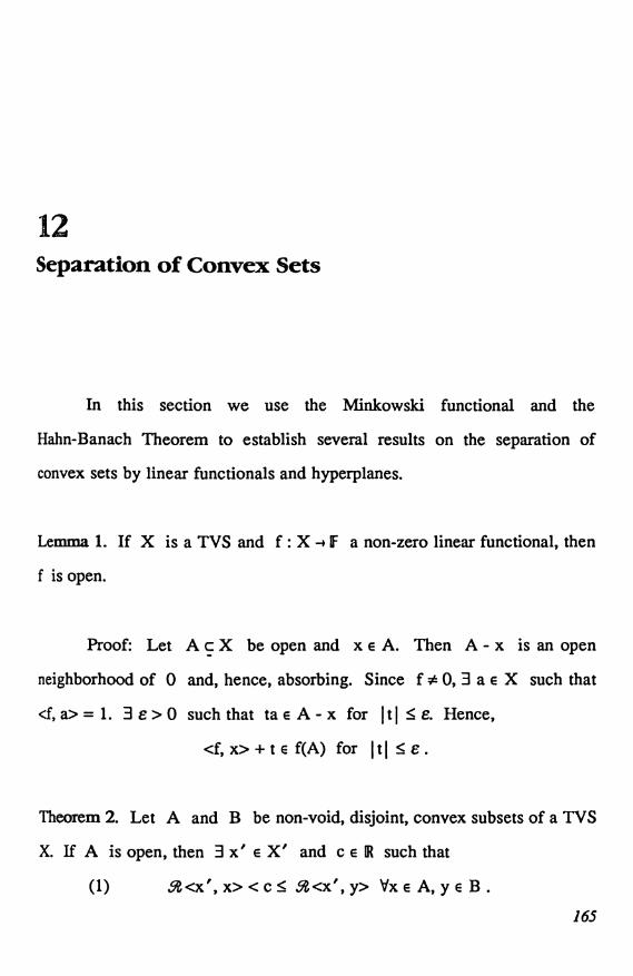
12

Separation of Convex Sets

In this section we use the Minkowski functional and the

Hahn-Banach Theorem to establish several results on the separation of

convex sets by linear functionals and hyperplanes.

Lemma 1. If X is a TVS and f : X -4 F a non-zero linear functional, then

f is open.

Proof: Let A c X be open and x E A. Then A - x is an open

neighborhood of 0 and, hence, absorbing. Since f : 0, 3 a E X such that

<f, a> = 1. 3 E> 0 such that tae A - x f o r I t I :5e. Hence,

<f,x>+tE f(A) for It <_e.

Theorem 2. Let A and B be non-void, disjoint, convex subsets of a TVS

X. If A is open, then 3 x' E X' and c e Qt such that

(1) ,5, <x', x> < C:5 A <X', y> VX E A, y e B .

165

166 Separation of Convex Sets

Proof: First, assume F = R. Fix a0 E A, bO a B. Put x0 = bO - a0,

C = A - B + xO. Then C is an open convex neighborhood of 0 such that

x0 9 C since A and B are disjoint. Let p be the Minkowski functional

of C. Note p(xO) >_ 1 by 11.13.

Let M = span{ xO } and define f on M by <f, txO> = t. If t >_ 0,

then <f, txO> = t<_ tp(xO) = p(txO); if t < 0, then <f, txO> = t<_ p(tx0).

Thus, f <_ p on M. By the Hahn-Banach Theorem (8.2), f has a linear

extension, x', to X which satisfies x' <_ p on X. In particular, x' <_ 1

on C so x' >_ -1 on -C. Hence, I x' S 1 on the neighborhood C n (-C)

of 0 and x' is continuous (Exer. 5.12).

If a E A and b E B, then

<x',a>-<x',b>+1=<x',a-b+xO>Sp(a-b+xO)<1

by 11.13. Hence, <x', a> < <x', b>. Thus, x'(A) and x'(B) are disjoint,

convex subsets of IR and x' (A) lies to the left of x' (B). x' (A) is open

by Lemma 1 and is, therefore, an open interval in R. Pick c to be the

right hand endpoint of x' (A).

If F = C, by the first part there is a real-linear continuous functional

f on X satisfying (1). Put <x', x> = <f, x> - i<f, ix> (8.3).

If f is a non-zero linear functional on a vector space X, then any

level set of f, {x : f(x) = c), is called a hyperplane. In Theorem 2, the set

A lies in the open half-space {x : <x', x> < c) and B lies in the closed

half-space {x : <x', x> >_ c) and the closed hyperplane

H={x:<x',x>=c}

is said to separate A and B.

Without some additional assumption on the convex sets it may not

Chapter 12 167

be possible to separate the convex sets by a hyperplane.

Example 3. In c00, let K = { {ti} : last non-zero ti is positive). Let f

be any non-zero linear functional on c00. Then <f, ek> * 0 for some k.

Then tek + ek+l E K f o r any t E U and

<f, tek + ek+l> = t<f, ek> + <f, ek+l>

may take on any value by choosing t appropriately. Note 0 f K so {0}

and K cannot be separated by any non-zero linear functional.

It is of interest, particularly in optimization theory, to know that

arbitrary disjoint convex subsets of IRn can always be separated by

hyperplanes ([Fr] 6.3).

Exercise 1. If B in Theorem 2 is also open, show that A and B can be

strictly separated in the sense that 3 3 > 0 such that

58<x',x>Sc-S<c<c+S<_ .5 <x',y> VxEA,yB.

13

Locally Convex TVS

Definition 1. A TVS (X, ,r) is a locally convex TVS (LCS) or r is alocally convex topology if and only if has a neighborhood base at 0

consisting of convex sets.

Example 2. Any semi-NLS is a LCS.

Example 3. Let 9' be a family of semi-norms on a vector space X. Let

a(X, 9') be the weakest topology on X such that each semi-norm p E 9

is continuous. Thus, a net {xs} in X converges to 0 in a(X, 9') if

and only if p(x& - 0 by E Y. The subsets, U, of the form

U= {x:p(x)<e,pE '90},

where e > 0 and 9'0 is a finite subset of 9, form an open neighborhood

base at 0 for o(X, 9). Thus, o(X, 9') is a locally convex topology for

X. Note o(X, P) is Hausdorff if and only if d x * 0 3 p e 9 such that

169

170 Locally Convex TVS

p(x) # 0, i.e., if and only if .}' separates the points of X. A net (x3) in

X is a Cauchy net in o(X, .9>) if and only if for every E > 0 and every

p e .' 3 S such that a, 0 ? S implies that p(xa - xp) < e.

We show below in Theorem 6 that Example 3 is a canonical

example in the sense that every locally convex topology is o(X, .0) for

some family .511.

Lemma 4. If U is an open, convex neighborhood of 0 in the TVS X,

then U contains an absolutely convex open neighborhood of 0.

Proof: U contains an open, balanced neighborhood, V, of 0. Set

W = coV. Then W is an open neighborhood of 0 (11.8), and since V is

balanced, W is absolutely convex (Exer. 11.4) with W c U.

Theorem 5. If X is a LCS, then X has an open (closed) neighborhood

basis at 0 consisting of absolutely convex sets.

Proof: The statement about open sets follows from Lemma 4 and

Exer. 11.5.

Let U be a closed neighborhood of 0 in X. By Exer. 11.5 and

Lemma 4 3 an absolutely convex neighborhood, V, of 0 such that

V c U. Then V c U and V is absolutely convex (11.8).

Chapter 13 171

Theorem 6. If (X, z) is a LCS, then r = o(X, ,9) for some family of

semi-norms Y.

Proof: Let 2C be a neighborhood base at 0 of open, absolutely

convex sets. For U E 2C let pU be the Minkowski functional of U and

set 9= (pU : U e 21). If U E 2C, then U = {x : pU(x) < 11 (11.13) so

T c o(X, ,'). But, each pU is -r continuous (11.13) so c (X, .') c z.

Corollary 7. If (X, c) is a LCS, then ti = o(X, .P), where ,' is the

family of all continuous semi-norms on X.

We have the following criteria for continuity and equicontinuity in

LCS.

Theorem 8. Let X and Y be LCS and assume that 6(Y, Q) is the

topology of Y. Let T : Y - Y be linear [ 5 a family of linear maps from

X into Y]. Then T is continuous [Y is equicontinuous] if and only if

V q E Q 3 a continuous semi-norm p on X such that q(Tx) <_ p(x) V x

[V T E 7].

Proof: :: Clear.

. *: V = { y e Y : q(y) < 1 } is an open neighborhood of 0 in Y.

Therefore, 3 e > 0 and continuous semi-norms pl, ..., pn on X such that

TUcV [TUcV VTE 5], where U= {x:pi(x)<c,i=1,...,n}. That

is, q(Tx) < 1 V x e U [V T e 91. Put p(x) = (116) max pi(x). Then p is15 i <_n

a continuous semi-norm on X. If x E X and t is chosen such that

p(x) < t, then x/t r= U so q(T(x/t)) = t q(Tx) < 1 or q(Tx) < t [d T e 5].

Letting t - p(x) gives q(Tx) S p(x) [V T E Y].

This. result should be compared with 5.5 and 5.21 for NLS.

We next show that a LCS has a large dual space.

Theorem 9. Let X be a LCS and X0 a closed linear subspace with

x0 ¢ X0. Then 3 a continuous linear functional x' E X' such that

<x', x0> = 1 and <x', X0> = 0.

Proof: Let M = span(x0, X0). 3 an open, absolutely convex

neighborhood, V, of 0 such that (x0 + V) o X0 = 0. Let p be the

Minkowski functional of V. Thus, p is a continuous semi-norm and

V = (x : p(x) < 1) (11.13). Define m' on M by <m, tx0 + x> -= t,

where t e F, x E X0. We claim that I <m', m> S p(m)

V m = tx0 + x E M. If t = 0, this is clear; if t * 0, then

p(m)=P(tx0+x)= Jtjp(x0+x/t) _ ItI =I<m',m>j

since x0 + x/t a V. By the Hahn-Banach Theorem m' has a linear

extension x' to X satisfying I <x', x> <_ p(x) V x e X. Then X' E X'

by Theorem 8 and <x', x0>=1 and <x', X0> = 0.

Corollary 10. Let X be a Hausdorff LCS. If x0 *0, x0 E X, then 3

Chapter 13 173

x' E X' such that <x', x0> # 0. That is, the dual space X' separates the

points of X.

Proof: Put X0 = {0} in Theorem 9.

Example 11. It follows that the space LO[0, 1] (1p[0, 1], 0 < p < 1) is

not locally convex. In particular, the spheres {x x I < r} in L0[0, 1]

are not convex. (Recall Example 5.18.)

Theorem 9 and Corollary 10 should be compared with 8.1.2 and

8.1.4. Results analogous to 8.1.4 and 8.1.5 are given by the following two

propositions.

Proposition 12. Let X be a LCS and p a continuous semi-norm on X.

If x0 E X, 3 x' E X' such that <x6, x0> = p(x0) and I <x', x> p(x)

VXEX.

Proof: Let E = span { x0 } and define x' : E -+ F by

<x', tx0> = tp(x0).

Then I <x', x> ( <_ p(x) V x E E. By the Hahn-Banach Theorem x' can

be extended to a linear functional x' on X satisfying I <x', x> 1 _< p(x)

V X E X. X' E X' by Theorem 8.

Proposition 13. Let K be a closed convex subset of a Hausdorff LCS X

and x 0 K. Then 3 x' E X' such that

.5<x', x> > sup( A <x', y> : y e K).

If K is absolutely convex, x' can be chosen such that

(1) <x',x> > 1 _ SUP[ I<x',y>I : yE K) .

Proof: 3 an open absolutely convex neighborhood of 0, U, such

that (x + U) n K = 0. By 12.2 3 x' E X' and C E O such that

,5k<x',x>>c? A<x',y>dyE K.

This gives the first part. If K is balanced, then <x', K> is a balanced set

of scalars so

<x' , x> I >_ A <X', x> > c ? SUP ( 58 <X', y> : y E K)

=sup( I<x',y>I:yEK).

Multiplication of x' by a suitable scalar gives (1).

Proposition 13 has an interesting corollary pertaining to the closures

of convex sets.

Corollary 14. Let X be a vector space with two locally convex topologies,

it and r2, which have the same continuous linear functionals. A convex

set K c X is r1-closed if and only if it is r2 closed.

Proof: Suppose K is r1-closed and x 0 K1. By Proposition 13 3

a r1-continuous linear functional x' and 5 > 0 such that

I<x',x>I > I<x',y>I +s dyE K.

Then I <x', x> - <x', y> I >5 V Y E K. Hence, U= {y : I <x', y> I <3)

is a r2 neighborhood of 0 such that (x + U) n K = 0 and K is r2 closed.

Chapter 13 175

Bounded Sets in LCS:

Theorem 15. A subset B of a LCS X with topology a(X, ,') is

bounded if and only if p(B) is bounded d p r: Y.

Proof: Suppose B is bounded and p e Y. Let p also denote the

semi-norm topology induced by p. The identity (X, a(X, ,9)) - (X, p) is

continuous so the implication follows from 5.3.

Let U be a neighborhood of 0 in X. Then 3 e > 0,

pl' "" Pn E 9) such that (x : pi(x) < e, i = 1, ..., n} c U. 3 M > 0 such

that pi(x) < M. V x E B, i = 1, ..., n. Hence (F/M)B c U and B is

a(X, ,9) bounded.

Analogous to 9.12, we have

Theorem 16 (Mackey). Let (X, z) be a LCS. A subset B c X is bounded

if and only if <x', B> is bounded d x' E X'.

Proof: *: 5.3.

: By Theorem 15 it suffices to show that p(B) is bounded for

each continuous semi-norm p on X, i.e., B is bounded in the semi-NLS

(X, p). By 9.12, B is bounded in (X, p) if and only if <x', B> is

bounded d x' E (X, p)'. But (X, p)' c (X, v)' so <x', B> is bounded

V x' E (X, p)' by hypothesis.

Recall that a sequence (xk) in a TVS X is said to be a Cauch

sequence if b neighborhood of 0, U, in X 3 N such that j, k ? N

implies J - xk E U. If X is a LCS, this is equivalent to the requirement

that `d continuous semi-norm p on X and for each e > 0 3 N such that

j, k >_ N implies p(xJ

- xk) < E. (See Example 3.) We say that a subset A

of a TVS X is sequentially complete if every Cauchy sequence in A

converges to a point of A. For sequentially complete LCS, we have the

following criterion for X boundedness.

Proposition 17. Let X be a LCS. If A c X is absolutely convex,

bounded and sequentially complete, then A is X bounded.

Proof: Let (xj } c A and tj -4 0. Given any subsequence of ( ),W

pick a further subsequence (tn) satisfying I to 15 1. Let p be aJ j=1 J

kcontinuous semi-norm on X. The partial sums, sk = to xn , form a

j=1 J J

Cauchy sequence in A since each Sk E A ande e

P ( Y' k - 9 c e ) 5 I to I P(xn) 5 sup (p(xi) : i E [N} I I tn. I

j=k+l J j=k+1 J00

for k < l (Theorem 15). Thus, the series tx n.

to a pointj=1 J J

in A, and A is X bounded.

The absolute convexity is important; see Exercise 20.3.

Corollary 18. If X is a sequentially complete LCS, then X is an

Chapter 13 177

A-space (§4).

This result now gives us a large number of examples of .A-spaces

(§4) and, thus, spaces for which the UBP holds (§9). Klis's example of a

non-complete normed X-space shows that the converse of Corollary 18 is

false ([KUJ).

Convex Hulls of Compact Sets:

Recall that a subset E of a metric space X is totally bounded or

precompact if d E> 0 3 a finite set F c X such that

Ecu[S(x,c):xeF),where S(x, e) is the E-sphere centered at x ([DS]). This idea is readily

generalized to TVS.

Definition 19. A subset E of a TVS X is precompact or totally bounded

if d neighborhood of 0, U, in X 3 a finite set F such that E c F + U.

Theorem 20. If X is a LCS and E c X is precompact, then coE is

precompact.

Proof: Let U be a neighborhood of 0 in X. Then 3 a convex

neighborhood of 0, V, in X such that V + V e U, and 3 a finite set F

such that E c F + V. Let El = coE, F1 = coF.

If (yl, ..., yn) are the points of F, then F1 is the image of then

compact set [ (t1, ..., tn) : ti >_ 0, ti = 1) C [Rn under the mappingi=1


n

(t1, ..., tn) and is, therefore, compact.

i=1k k

If X E El, then x = sixi, where si >_ 0, ) Si = 1 and xi E E.

i=1 i=1

For each i; 3 zi E F such that xi - zi e V. Decompose x into a sumk k

x = xl + x2, where x1 = sizi, x2 = si(xi - zi). Now x1 E F1 and

i=1 i=1

x2 E V since V is convex. Thus, El c F1 + V. But, F1 is compact so 3

a finite set F2 such that F1 c F2 + V (Exer. 5). Hence,

El CFI+V+VcF2+U

and E1

is totally bounded.

From Theorem 20, we obtain a result of Mazur.

Corollary 21 (Mazur). Let X be a complete metrizable LCS. If E c X is

compact, then -c-oE is compact.

Proof: Recall that a subset of a complete metric space is compact if

and only if it is closed and precompact ([DS]); apply Exer. 5.

It is interesting to note that the convex hull of a compact subset of a

finite dimensional space is compact ([Ru] 3.25). The completeness in

Corollary 21 is important (see Exer. 6).

Completion of a LCS:

Chapter 13 179

Let E be a Hausdorff LCS whose topology is generated by the

family of semi-norms 9'. For P E 9 let Np = {x : p(x) = 0). Form the

quotient space Ep = E/Np and denote the coset x + Np = xp. Equip EP

with the quotient norm p from p, p(xp) = p(x) (6.4), and let Fp be the

completion of Ep under p (8.1.14). Form the product space F = IIFp

for p E Y; F is then a complete LCS (Exer. 1.9 and Exer. 13).

With any x E E associate the element x = (xp) of F. The map

x -4 x is 1-1, linear and is a homeomorphism from E onto a linear

subspace E of F. This construction shows that any Hausdorff LCS can

be imbedded in a product of B-spaces. The closure of E in F then

furnishes a completion of E. Furthermore, it is easy to see that E is

complete if and only if E is closed in F.

Exercise 1. If 9:) £, show -0) ? o(X, L). Show that it is possible

to have ooX, P) = o(X, .£) with ,' # L.

Exercise 2. If X is a LCS whose topology is induced by a sequence of

semi- norms {pk), show 3 a sequence of semi-norms {pk) such that

and (pk) induces the same locally convex topology as the

Exercise 3. Let X be a TVS and (Y, o(Y, ,')) a LCS. If T : X -a Y is

linear, show T is continuous if and only if pT is continuous d p E Y.

Exercise 4. Let (X, cF(X, ,')) be a LCS and Z a linear subspace. Show

Z is a LCS with respect to the induced topology and the semi-norms

{p Z : p e P} generate the induced topology.

Exercise 5. Show a precompact set is bounded. Show a compact set is

precompact. Show the closure of a precompact set is precompact.

Exercise 6. Show Corollary 21 is false if completeness is dropped. [Hint:

Consider c00 with the l 2-norm. Let E = (e/k : k E 1N) u { 0). Pick

00 n n

tk > 0, tk = 1, and consider the vectors tk)-1 I tkel/k.]k=

=1 k=1 k=1

Exercise 7. Let X, Y be LCS and B : X x Y -4F bilinear. Show B is

continuous if and only if 3 a continuous semi-norm p(q) on X(Y) such

that I B(x, y) <_ p(x)q(y) d x E X, Y E Y.

Exercise 8. Let (tk) E e I. Let X, Y be LCS with (x') a X' and

(y1 } c Y' equicontinuous. Show B : X x Y -4R,00

B(x, y) = I tk<xk, x><yk, y>k=1

is continuous. Such bilinear forms are called nuclear.

Exercise 11. Let X be a Hausdorff LCS. Show that X is metrizable if

and only if its topology is induced by a countable number of semi-norms.

Exercise 10. If X is a LCS and M a linear subspace, show that M' is

Chapter 13 181

algebraically isomorphic to X'/M1, where

M''= (x' E X' : <x',nv=0 VmE M) .

Exercise 11. Let X be a LCS and M a linear subspace. Show that X/M

is a LCS under the quotient topology. If X is metrizable and M is

closed, show, X/M is metrizable.

Exercise 12. Let X, Y be Hausdorff LCS and T : X -+ Y a linear,

continuous, open mapping onto Y. If X is a complete metrizable space,

show that Y is also.

Exercise 13. Show that the product of LCS is a LCS. Describe the

semi-norms which generate the product topology.

Exercise 14. If B is a bounded subset of a LCS, show coB is bounded.

Exercise 15. Let E be a vector space and let 2l be the family of all

absolutely convex, absorbing subsets of E. Show 21 is a base for a

locally convex topology r on E; r is called the strongest locally covex

topology of E. Show:

(i) r is Hausdorff. [Hint: Use a Hamel basis.]

(ii) r is generated by the family of all semi-norms on E.

(iii) If F is a LCTVS and T : E -+ F is linear, show T is

continuous with respect to T.

(iv) Every r bounded set is finite dimensional.

(v) Every linear subspace is closed.

(vi) If E is infinite dimensional, r is not metrizable.

13.1 Normability

We now have the machinery available to characterize normable

TVS. It turns out that the simplest necessary condition is also sufficient.

Theorem 1 (Kolmogorov [K]). Let X be a Hausdorff TVS. The topology

of X is induced by a norm (i.e., is normable) if and only if X contains a

bounded, convex open neighborhood of 0.

Proof: Clear.

a: Let U be a bounded, open convex neighborhood of 0. Then 3

an absolutely convex open neighborhood of 0, V, such that V c U (13.4).

V is clearly bounded. Let p be the Minkowski functional of V.

Now p is a norm; for if x * 0, then since X is Hausdorff 3 a

balanced neighborhood W of 0 such that x E W. Since V is bounded,

3 t > 0 such that V c tW. There exists s > p(x) so that x e sV. Then

x/s e tW or x E stW. Since W is balanced and x it W, st > 1 or s > 1/t

and p(x) >_ 1/t > 0.

Next we claim that the topology induced by p (and denoted by p)

coincides with the original topology, T, of X. Since V is bounded, if W

is a r -neighborhood of 0 3 e > 0 such that EV c W. Hence, (eV : e > 0)

is a base at 0 for T. Since V = {x : p(x) < 1), (eV : e> 0) is also a

base at 0 for p and p = z

Corollary 2. A bounded set in a non-normable Hausdorff LCS X is

nowhere dense.

Chapter 13 183

Proof: Suppose B is bounded and xo E int(B). 3 an open convex

neighborhood of 0, U, such that x0 + U c B. Then U c -x0 + B implies

that U is bounded and X is normable by Theorem 1.

Corollary 3.. A complete, quasi-normed Hausdorff LCS X is normable if

and only if X is a countable union of bounded sets.

Proof: *: Clear.Co

If X = u Bn with Bn bounded, some Bn is not nowheren =l

dense by the Baire Category Theorem. X is normable by Corollary 2.

13.2 Krein-Milman Theorem

Let X be a vector space and K c X. A subset E c K is an

extremal subset of K if E * 0 and whenever x, y e K and 0 < t < 1

implies tx + (1 - t)y E E, then x, y E E. An extremal point (or extreme

in of K _ is an extremal subset consisting of the point. Thus, a point

x E K is an extreme point of K if x = tx 1 + (1 - t)x2 with xi E K,

0 5 t <_ 1, implies xl = x2 = x. It is easy to see that if E1 is an extremal

subset of an extremal subset E2 of K, then E1 is an extremal subset of

K.

Example 1. In IR2, the extreme points of ((x, y) : II (x, y) I I 1 S 1) are

(±1, 0) and (0, ±1); the extreme points of ((x, y) : lix, Y)112 5 11 are

{(x, Y) : II(x, Y)112 =1}.

In this example the sets are the closed unit balls of NLS. All such

balls don't have extreme points.

Example 2. Let K = { { tk } E co : II (tk) II 5 1) . Then K has no extreme

points. It is clear that an interior point of any convex subset of a TVS

cannot be an extreme point so let {tk} E K with II {tk} II = I.

Select any t. with It.I < 1/2. Define x = (xk) , y = {yk} E K by

Yk = X k = tk if k ;&j and x1 = ti + 1/2, yj = t1 - 1/2. Then

lx+7y= {t.} and x#y.

Further examples of extreme points in function spaces are given in

the exercises.

Note in Example 1 that the compact convex sets considered are the

Chapter 13 185

convex hulls of their extreme points. The Krein-Milman Theorem gives a

general relation between a compact convex set and the convex hull of its

extreme points.

Lemma 3. Let K * 0 be a compact subset of a Hausdorff TVS X. For

x' E X' let a = sup { 5<x', x> : x E K). Then

E=(XEK: . <x',x>=a)

is an non-empty, compact, extremal subset of K.

Proof: Since K is compact, E is non-empty and compact.

Suppose x, y E K, 0 < t < 1 and tx + (1 - t)y E E. Then

a = 5t<x', tx + (1 - t)y> = t 5E<x', x> + (1 - t) 5Z<x', y>

and since ,5 , <x', x> <_ a, A <x', y> <_ a, we must have

A<x',x>= .5 <x',y>=a and x,yeE.

Theorem 4. Let K be a non-empty compact subset of a Hausdorff LCS

X. Then K has at least one extreme point.

Proof: Let 9 be the family of all non-empty, compact extremal

subsets of K. Then 9 * 0 since K E 9. Partially order 9 by reverse

set inclusion; E1 S E2 if and only if E1 : E2. If sB is any chain in ',

then n s'= E is non-empty since K is compact and E is an upper bound

for 6. By Zorn's Lemma X has a maximal element E0. We claim that

E0 must be a singleton, establishing the result. Since E0 cannot contain a

proper non-empty compact extremal subset, it follows from Lemma 3 that

Ax' must be constant on E0 V x' E X'. By 13.10, E0 must be a

singleton.

Theorem 5 (Krein-Milman). Let K be a non-empty compact subset of a

Hausdorff LCS X. Then K is contained in the closed convex hull of its

extreme points.

Proof: Let H be the closed convex hull of the extreme points of

K. Suppose 3 x E K\H. By 13.13 3 x' E X' such that

SUP( A<x',y>:yE H) < 58<x', x>.

If a=sup( A<x',y>:yEK) and E=(yEK: A<x',y>=a),H n E = 0. Now E is non-empty and compact so E has an extreme point

x0 by Theorem 4. E is an extremal subset of K by Lemma 3 so x0 is

an extreme point of K. Since H n E = 0, this is impossible. Hence,

K c H.

Corollary 6. If K is a non-empty, convex compact subset of a Hausdorff

LCS X, then K is the closed convex hull of its extreme points.

Despite its somewhat esoteric appearance, the Krein-Milman

Theorem has a surprising number of applications. We give such

applications to the existence of preduals for NLS, Liapounoff s theorem on

the convexity of the range of a vector measure and the Stone-Weierstrass

Theorem in § 15.

Another interesting application of the Krein-Milman Theorem which

Chapter 13 187

we will not give is to a result of Banach and Stone which we now describe.

If S and S' are compact Hausdorff spaces such that C(S) and C(S')

are linearly isometric, then the Banach-Stone Theorem asserts that S and

S' are homeomorphic; for a proof use [DS] V.8.8.

Exercise 1. Show the set of extreme points of a compact convex set needn't

be compact. [Hint: In IR3, consider the convex hull of (1, 0, ±1) and

(cos t, sin t, 0) 0<_t<_27r.]

Exercise 2. Show the closed unit ball of L1[0, 1] has no extreme points.

c[Hint: If IIf II 1 = 1, pick c such that Jifi = 1/2 and consider [0, c),

0

Exercise 3. Show f E L"[0, 1] is an extreme point of the closed unit ball

if and only if f(t) = 1 a.e.

Exercise 4. Show compact cannot be replaced by closed and bounded in

Theorem 4.

Exercise 5. Show (tek : I t 1, k E II) are the extreme points of the

closed unit ball of l

Exercise 6. If S is a compact Hausdorff space, show the extreme points of

the closed unit ball of C(S) consists of those functions with I f(t) I = 1

V t E S.

Exercise 7. Show the extreme points of the closed unit ball of Lp[O, 1]

consists of those functions with IIfIIp = 1 provided 1 < p < oo.

Exercise 8. Show the closed unit ball of c has two extreme points,

x = (1, 1, ...) and -x.

14Duality and Weak Topologies

We next consider an abstract construction that can be used to define

important locally convex topologies, called weak topologies, on vector

spaces.

If X is a vector space, its algebraic dual, the set of all linear

functionals on X, will be denoted by X#.

Definition 1. Let X, Y be vector spaces (over F) and b : X x Y --3 F

bilinear. Then X and Y are said to be in duality (with respect to b) if

(i) {b(, y) : y E Y, Y :A 0) separates the points of X,

(ii) (b(x, ) : x E X, x * 0) separates the points of Y.

Example 2. Let X be a vector space. Then X and X# are in duality

with respect to the natural bilinear mapping, b(x, y) = y(x) _ <y, x>,

between X and X. Actually if Y is any linear subspace of X which

189

190 Duality and Weak Topologies

separates the points of X, then X and Y are in duality with respect to

Example 3. If X is a Hausdorff LCS, then X and X' are in duality as

in Example 2 (13.10).

Suppose that X and Y are in duality. For each y E Y,

y# = b(-, y) defines an element of X# and from (ii) the map y -+ y#

defines an isomorphism of Y into X. Therefore, we may consider Y to

be a linear subspace of X# which separates the points of X with the

bilinear mapping between X and Y to be the natural bilinear pairing

given in Example 2. Henceforth, we adopt this notational convenience.

Let X and Y be in duality. To each y E Y, there is associated a

semi-norm py on X defined by py(x) = I <y, x> 1. The locally convex

topology a(X, {py : y E Y}) is called the weak topology on X (from the

duality between X and Y) and is denoted by g (X. Y). We have the

following properties of the weak topology (13.3).

Proposition 4. (i) o(X, Y) is the weakest topology on X such that all the

elements of Y are continuous.

(ii) A base at 0 consists of (x : <yi, x> I < e, i = 1, ..., k},

where y1, ..., yk E Y and E > 0.

(iii) A net {x3} in X converges to 0 in a(X, Y) if and

only if <y, xba - 0 d y e Y.

(iv) a(X, Y) is Hausdorff (Definition 1.(i)).

(v) A sequence (xk) in X is a(X, Y) Cauchy if and only if

Chapter 14 191

V Y E Y (<y, xk> ) is Cauchy.

It follows from Proposition 4 (i) that the dual of (X, a(X, Y))

contains Y; we now show that the dual is exactly Y.

Lemma 5. If g * 0 and fl, ..., fk are linear functionals on the vector

space X, then either g is a linear combination of {fl, ..., fk} or else

3 x0 E X such that <g, xO>=1 and <i, xO>=O for i = 1, ..., k.

Proof: We may assume that {fl, ..., fk} is linearly independent.

For k = 0 the result is trivial; assume that it holds for k S n - 1. Then for

each i, 1 <_ i <_ n, f. is not a linear combination of (f..: 1 S j _< n, j i) so

by the induction hypothesis 3 ai E X such that <fj, ai> = Sij, i = 1, ..., n.

n nFor each x E X, x- <f-, x>ai E K = n ker i. Then either 3 a E K such

i=1 i=1

that <g, a> = 1 (and <fi, a> = 0 i = 1, ..., n) or <g, a> = 0 V a E K. Inn n

the latter case, V X E X <g, x> _ <f., x><g, a> and g = <g, ai>f..

i=1 i=1

Theorem 6. Let X and Y be in duality. Then the dual of (X, o(X, Y))

is Y.

Proof: Let f be a linear functional on X which is continuous with

respect to a(X, Y). Then <f, x> t < 1 on some neighborhood, U, of

0 of the form U=(x: <y1,x> Se,i=1,...,n), yi Y, e>0. By

Lemma 5, either f is a linear combination of yl, ..., yn or 3 a E X such

that <f, a> = 1 and I <yi, a> I = 0, i = 1, ..., n. But in the latter case,

a e U and <f, a> = 1 > t. Hence, f e Y.

If X and Y are in duality, then certainly Y and X are in duality

so (Y, a(Y, X))' = X by Theorem 6.

Example 7. If X is a Hausdorff LCS, then (X, a(X, X'))' = X' and

(X', a(X', X))' = X. In this situation, o(X, X') is called the weak

topology- of X and a(X', X) is called the weak* top to ogy of X'.

Definition 8. Let X and Y be in duality. A locally convex Hausdorff

topology r on X is said to be compatible with the duality between X

and Y if (X, T)' = Y.

By Theorem 6, o(X, Y) is such that topology, and it is the weakest

such topology.

Example 9. Let X be a non-reflexive B-space. Then X' and X are in

duality. On X the topology o(X, X') and the norm topology are

compatible with respect to this duality. On X' theweak*

topology

a(X', X) is compatible with the duality between X' and X, but the norm

topology and the weak topology o(X', X' ) on X' are not compatible

with this duality since their duals are X" # X.

Chapter 14 193

From 1-3.14 we have the following important property of the

closures of convex sets with respect to the weak topology.

Theorem 10. Let X and Y be in duality. If K c X is convex, then the

closure of K is the same for any locally convex topology which is

compatible for the duality between X and Y.

In particular, if (X, r) is a Hausdorff LCS, then any convex subset

of X is r -closed if and only if it is o(X, X') closed.

Continuity of Linear Operators with respect to Weak Topologies:

Theorem 11. Let X and Y be Hausdorff LCS and T : X -4Y linear. If

T is continuous with respect to the original topologies of X and Y, then

T is continuous with respect to a(X, X') and a(Y, Y').

Proof: Let (xs) be a net in X which is a(X, X') convergent to

0. If y' e Y', then y'T E X' so <y', Tx8> -40 or (Tx5) is o(Y, Y')

convergent to 0.

The converse of Theorem 11 is false. To show this we need a

preliminary observation.

Lemma 12. Let X and Y be in duality. If X is infinite dimensional,

every o(X, Y) neighborhood of 0 contains an infinite dimensional

subspace of X.

Proof: Let U= (x: I<yi,x> SE,i=1,...,n),yiEY,E>0,bean

basic o(X, Y) neighborhood of 0. Then L = n ker yi is a lineari=1

subspace of co-dimension at most n which is contained in U.

Corollary . 13. If X is an infinite dimensional NLS, then the weak

topology of X, o(X, X'), is strictly weaker than the norm topology of X

and is not normable.

We can now show that the converse of Theorem 11 is false.

Example 14. Let Y be an infinite dimensional NLS. Take X to be Y

equipped with the weak topology o(Y, Y'). Then the identity map from

X onto Y is o(X, X') - o(Y, Y') continuous but is not continuous with

respect to the original topologies of X and Y by Corollary 13.

We can establish a partial converse to Theorem 11. For this we

need the following important observation concerning bounded sets.

Theorem 15 (Mackey). Let (X, i) be a Hausdorff LCS. A subset B c X

is z bounded if and only if it is o(X, X') bounded.

Proof: 13.16.

Thus, any two locally convex topologies which are compatible with

Chapter 14 195

the duality between X and X' have the same bounded sets. However,

two locally convex topologies can have the same bounded sets and not be

compatible (see 16.8).

Proposition 16. Let X, Y be Hausdorff LCS and T : X - Y linear. If T

is o(X, X') - o(Y, Y') continuous, then T is bounded with respect to the

original topologies of X and Y.

Proof: T is bounded with respect to the weak topologies of X and

Y (5.3) so the result follows from Theorem 15.

Corollary 17. Let X, Y be Hausdorff LCS and T : X -+ Y linear. If X

is quasi-normed and T is o(X, X') - 6(Y, Y') continuous, then T is

continuous with respect to the original topologies of X and Y.

Proof: Proposition 16 and 5.4.

We will give a generalization of this result to more general domain

spaces in §21.

We can now give an example of a bounded linear operator which is

not continuous (see 5.3).

Example 18. Let X be an infinite dimensional NLS. The identity

operator from (X, o(X, X')) onto (X, is bounded (Theorem 15) but

not continuous (Corollary 13).

,A-spaces which are not_ -spaces:

The results above can be used to give examples of .A-spaces which

are not X-spaces (§4). For this we require a preliminary observation.

Lemma 19. Let X and Y be in duality, and let a, be two locally

convex topologies on X which are compatible with the duality between X

and Y and assume a c T. If (X, r) is an /kspace, then (X, a) is an

.A-space.

Proof: The identity map from (X, r) onto (X, a) is continuous so

the result follows from Theorem 15 and Exer. 5.13.

Example 20. If X is a B-space, then (X, a(X, X')) is an at-space by

Lemma 19. In particular, if X = l p, 1 < p < -, then (X, a(X, X')) is an

,4-space but is not a X-space [consider the unit vectors eki.

Exercise 1. If r is a locally convex topology lying between two

compatible topologies, show r is compatible.

Exercise 2. If X is finite dimensional and X and Y are in duality, show

Y is finite dimensional and dim X = dim Y.

Exercise 3. Let X be a Hausdorff LCS and L a linear subspace of X'.

Show L is a(X', X) dense in X' if and only if L separates the points

of X.

Chapter 14 197

Exercise 4. Let X be a NLS. Show a(X, X') is metrizable if and only

if o(X, X') is normable if and only if X is finite dimensional.

Exercise 5. Let X and Y be in duality and M a linear subspace of Y

which separates the points of X with M # Y. Show a(X, Y) is strictly

stronger than o(X, M).

Exercise 6. Let X be a Hausdorff LCS and M c X a linear subspace.

Show o(M, M') and the relative a(X, X') topology on M coincide.

Exercise 7. Let X be a B-space. When is o(X', X) = a(X', X")?

Exercise 8. Compare the metric and weak topologies of s.

Exercise 9. Does the analogue of Corollary 13 hold for quasi-normed

spaces?

Exercise 10. In (12, a(l2, 12)) show (ek) converges to 0 but is not

Mackey convergent to 0.

Exercise 11. Let X be a Hausdorff LCS and M a linear subspace. Show

that a(X/M, (X/M)') is a(X, X') I M (see Exer. 6.4).

Exercise 12. Let E be a vector space and E# its algebraic dual. Show

that E# is complete under a(E#, E).

15The Bipolar andBanach-Alaoglu Theorems

In this section we establish two very important results for weak

topologies, the Bipolar Theorem and the Banach-Alaoglu Theorem. We use

these results along with the Krein-Milman Theorem to prove the Liapounoff

Theorem on the range of a vector-valued measure and a generalization of

the Stone- Weierstrass Theorem due to de Branges.

Let X and Y be in duality.

Definition 1. Let A c X. The polar of A (with respect to the duality

between X and Y), A0, is defined by {y E Y: <y, x> 5 1 V X E A}.

Let B c Y. The polar of B, BO, is defined by

{XEX: J<y,X>1 1 VyEB}.

The notation is designed to help indicate the space in which the

polars are being computed. If X and Y are in duality, we think of X as

being the "ground space" and Y the "dual" or "upstairs space" as in the

199

200 The Bipolar and Banach-Alaoglu Theorems

diagram below

Y AO B

X A B0

If A is a subset of the ground space, AO is computed in the upstairs

space; if B is a subset of the upstairs space, B0 is computed in the ground

space.

Example 2. Let X be a NLS. Consider the duality between X and X'.

If S = (x : lIxII <_ 1), then SO = (x' E X' : jjx' 11 S 1); if

S' = (X'EX':IIX'I 51),then (S' )0 = S. Note in this example that (SO)0 = S and ((S' )0)0 = S'.

The Bipolar Theorem gives a general form of this phenomena.

Polars satisfy the following elementary properties.

Proposition 3. Let A, B c X.

(i) If A c B, then BO ? AO.

(ii) A c (A0)0 and AO = ((A°)0)°.

(iii) AO is absolutely convex and o(Y, X) closed.

(iv) If t e F, t * 0, then (tA) 0 = (1/t)A0.

(v) If H is the o(X, Y) closed, absolutely convex hull of A,

then HO = AO.

Proof: (i) is clear.

(ii): If a E A, then for a' E AO, I <a', a> 1 <_ 1 so a E (A0)0 and

Chapter 15 201

A c (AO)0. By the first part ((A°)0)0 o AO and by (i) AO :) ((A°)0)°.

(iii): The absolute convexity is clear and

AO = n [X' E Y : I<X', x> I <_ 1)xE A

implies AO is 6(Y, X) closed since each x e A is a(Y, X) continuous.

(iv): Let X' E (1/t)A0. For x e tA, x = to for some a E A. Also

x' = (1/t)y' with y' E AO. Hence, I <x', x> _ <y', a> 1 and

x' E (tA)0. Hence, (1/t)A0 c (tA)0. Now (tA)O = (1/t)t(tA)0 c 1/t(A0).

(v): From (iii) and (ii), A c H c (A0)0; by (i) and (ii),

AO : HO ((AO)O)O = AO.

Proposition 4. A c X is a(X, Y) bounded if and only if AO is absorbing

in Y.

Proof: Suppose A is o(X, Y) bounded. Let X' E Y. Then

t = sup (l<x' , x> l : x E A) <-. If t = 0, x' E A0; if t > 0, then for

Is 51/t, sx' E AO so AO is absorbing.

Suppose AO is absorbing. Let X' E Y. Then 3 t > 0 such that

x' E tAO. Then ( <x', x> 1 5 t d x E A and A is a(X, Y) bounded.

Theorem 5 (Bipolar Theorem). Let X and Y be in duality. For A C X,

(A0)0 is the o(X, Y) closure of the absolutely convex hull of A. In

particular, if A is o(X, Y) closed and absolutely convex, then

A = (AO)0.

Proof: Let H be the o(X, Y) closure of abcoA. By Proposition

3 (A°)0 ? H. Suppose 3 x E (A0)0\H. By Lemma 13.13, 3 x' e Y such

that <x', x> > 1 and I<x', a> l <_ 1 d a E H. Since H A, x' E AO so

x o (A°)0.

We now prove an important compactness result for weak topologies,

the Banach-Alaoglu Theorem.

Lemma 6. Let X be a vector space and Y a linear subspace of X#

which separates the points of X. Then Y CIIF = FX and the topologyX

a(Y, X) and the induced product topology on Y from IIIF coincide.X

Proof: A net (y3} in Y converges to y E Y in either topology if

and only if <y6, x> -* <y, x> V X E X.

Theorem 7 (Banach-Alaoglu). Let X and Y be in duality. Suppose r is

a compatible topology on X. If U is a neighborhood of 0 in X, then

U0 c Y is a(Y, X) compact.

Proof: By Proposition 3 we may assume that U is a(X, Y) closed

and absolutely convex. By 14.10, U is also -r-closed.

Let p be the Minkowski functional of U. We claim that

UO = {x' E Y : <x', x> p(x) V x E X). For if x' E Y is such that

I <x', x> I <_ p(x) V x E X, then for x E U I<x', x> <_ p(x) 5 1 (11.13),

Chapter 15 203

so x' E U0. On the other hand, if x' E U0 and x e X with p(x) > 0,

then x/p(x) E U (11.13) so I <x', x> S p(x), and if p(x) = 0, then

nx E U d n >_ 1 so I<x', x> <_ 1/n and I<x', x> = 0 = p(x).

For X E X, set D(x) = [t E F : It 5 p(x) }. From above

U0 C H D(x) and from Lemma 6 the a(Y, X) topology on U0 is theXEX

relative product topology on U0 from the product E F. From Tychonoff sX

Theorem U0 is relatively compact in the product topology so it suffices to

show that U0 is closed in the product topology. Let j x') be a net in

U0 such that xs -* f E HF in the product topology. f is clearly linear and

<f,X> p(X) VXEX

so f is also continuous since p is 'r continuous (11.13). Hence,

f E U0 and U0 is closed in the product topology.

Corollary 8. Let X be a NLS. The closed unit ball,

S'= (X'EX':llX'11 51),

of X' is weak* (a(X', X)) compact.

Proof: Theorem 7 and Example 2.

From 8.1.6, we obtain

Corollary 9. Let X be a NLS. Then X is linearly isometric to a

subspace of C(S'),'), where S' = (x' : IIx' jI <_ 1) has the weak* topology.

Corollary 8 is false for the unit ball of a NLS (or even a B-space)

and the weak topology. In fact, the unit ball of c0 is not compact for any

locally convex topology on c0. For if this were the case, the closed unit

ball of c0 would have extreme points by the Krein-Milman Theorem. In

Example 13.2.2 it was shown that the closed unit ball of co has no

extreme points.

In 5.8 it was shown that the dual of a NLS is a B-space under the

dual norm. It is reasonable to ask if every B-space is the dual of some

NLS, i.e., does every B-space have a 12redual. From the discussion above it

follows that c0 is not the dual of any NLS for if this were the case, the

unit ball of c0 would be weak compact and have extreme points.

We give another interesting and important application of the

Banach-Alaoglu and Krein-Milman Theorems to vector-valued measures.

Let E be a 6 algebra of subsets of a set S. A real-valued measure . on

E is non-atomic if every E e E with 0 < I X I (E) = var(A,)(E) contains a

subset A E E with 0 < I X 1(A) < J2 I (E). For example, Lebesgue measure

is non-atomic. Concerning the range of a non-atomic measure with values

in a finite dimensional space, we have the following result of Liapounoff.

Theorem 10 (Liapounoff). Let µl, ..., µn : E -i fR be countably additive

and non-atomic. If p.: E -4 IRn is given by µ(E) = (µ1(E)' "" µn(E)), then

µ(E) is a convex, compact subset of fRn.

n

Proof: Let A _ 1 µi and note that X is non-atomic. Definei=1

Chapter 15

Jgd/ln)

205

T : L°°(A) - IRn by Tg = (isgdp,, ..., (note T is well-defined

since each Ai is absolutely continuous with respect to A). By the Radon-

Nikodym Theorem, T is continuous with respect to the weak topology of

L°°(A) and the norm topology of IRn.

Put K = (g e L°°(A) : 0:5 9:5 1). Now KrS is convex and is weak*

closed since g c- K if and only if 0:5is

fgdA. <_J

fdA. V f ? 0, f E L1(A).J

Since K is contained in the closed unit ball of C(A), K is weak*

compact by the Banach-Alaoglu Theorem. Thus, TK is compact in O.

We claim that µ(E) = TK establishing the result. If E E E, then

CE E K so T(CE) = µ(E) E TK, and µ(E) c TK. Suppose Y E TK and

set Ky = T-1(y). We must show that Ky contains the characteristic

function of a set in E. But Ky is weak closed so weak compact and is

convex. Therefore, by the Krein-Milman Theorem Ky has an extreme

point. We claim that such an extreme point must be a characteristic

function. For suppose g e Ky is not a characteristic function. Then

3 E E E and E> O such that A(E) > 0 and e e<_ g 5 1- e on E. If

L=CELc*(X), then since A(E) > 0 and A is non-atomic, L must be

infinite dimensional (Exer. 4). Therefore, 3 f E L, f # 0, such that Tf = 0

with -e<f<E. Then g±fE Ky, ±±' t-g and g = (g+f)+ (9-f)implies that g is not an extreme point of Ky.

Liapounoff s Theorem does not hold in general for infinite

dimensional B-spaces. Let Z be the Lebesgue measurable subsets of

[0, 1] and let m be Lebesgue measure on [0, 1]. Define µ : 1 -4 L1(m)

by µ(E) = CE. Then µ is countably additive and by the Dominated

Convergence Theorem, µ(E) is closed. However, µ(E) is not convex

[1/2 E coµ(E), but if E E E, then

111/2 - u(E)II1 = (m([0, 1]\E) + m(E))/2 = 1/2],

and also y(E) is not compact since if En = {t : sin 2nnt > 0], then

II/(E) - 4(Ek)II1 = 1/4 for j # k. Note that µ is non-atomic in the

(weak) sense that x'µ is non-atomic b x' E L°°(m).

Liapounoff s Theorem has important applications in control theory

so there is a great interest in obtaining infinite dimensional versions of the

theorem. For such generalizations, see [DU]; for applications of the

theorem to control theory, see [HL].

We give a further application of the Krein-Milman and Banach-

Alaoglu Theorems to the Stone-Weierstrass Theorem. Let S be a compact

Hausdorff space and let C(S) be the space of all complex-valued

continuous functions defined on S equipped with the sup-norm. The dual

of C(S) is the space, rca(S), of all regular, complex Borel measures on S

with the total variation norm, IIµII = var(,u)(S) = I µ I (S) (Example 5.16).

The support of a measure µ E rca(S) is the set of all t E S such that

I PL I (U) > 0 V open neighborhood U of t. The support is a closed set. If

the support of µ is empty, then V t E S 3 an open neighborhood U(= Ut)

of t such that I µ I (U) = 0 and since S is compact, S is a finite union of

such neighborhoods; it follows that µ = 0 if and only if the support of µ

is empty.

Notice that if A is linear subspace of a LCS E, then its polar is

0A= (x' EE' :<x',x>=0VxE A).

Chapter 15 207

Theorem 11 (de Branges). Let 4 be a subalgebra of C(S) and let

K = (µ e .40 : llµll <_ 1). Let µ be an extreme point of K and let f be

a real-valued function in .4 such that 0 < f < 1. Then f is constant on

the support of A.

Proof: If µ = 0, trivial. If A :t- 0, then 11µl1 = 1. Define A,

v e rca(S) by v(E) = J/2, A(E) = J(1 - f)dµ. Since f E , f and .4 is

an algebra, v, a, E ,40, and since 0 < f < 1, 2, and v are non-zero. Now

llvII(v/llvlI) + iIAlI(,VIiAlI) and

IIvII + IIAII = Jfthh1 I + is(1 - f)dlµl = lgl (S) = 1

so µ is a convex combination of v/Ilvll and A/11AII. Since µ is an

extreme point of K, µ = v/Il vil = )/IIAII or v = ll vllp. Hence,

v(E) = Jfdµ = fit viIdp. for each Borel set E, and since f is continuous,

f = it vll on the support of M.

Theorem 12 (Stone-Weierstrass). Let .4 be a closed subalgebra of C(S)

satisfying

(i) 1 E .4,

(ii) .4 separates the points of S and

(iii) f e 44 f E A. Then ,4= C(S).

Proof: Let K = (µ E .40 : 11µ1l _< 1). It suffices to show that

K = (0). Now K is non-void, convex and compact in the weak topology

by the Banach- Alaoglu Theorem. Hence, K contains an extreme point

µ(13.2.4). We claim that the support of µ is a singleton. Suppose s, t

belong to the support of M. By (ii) and (iii), 3 f E .4 such that 0 < f < 1

and f(s) 0 f(t). This is impossible by Theorem 11.

Thus, µ = t6s, where t E C and Ss is the Dirac measure or point

mass at s E S. However, µ E -90 so <µ, f> = tf(s) = 0 d f E 4 By (i),

t = 0 or µ = 0. By the Krein-Milman Theorem, K = (0).

Exercise 1. Show (uAa) 0 = rA0

Exercise 2. If s, t > 0, show (1/s A) 0 + (1/t A) 0 = (1/(s + t)A) 0.

Exercise 3. Does L1[0, 1] have a predual? (Hint: Exer. 13.2.2.)

Exercise 4. If A. is a non-atomic, positive measure, show L°°(2,) is

infinite dimensional. Can the non-atomic assumption be dropped?

Exercise 5. Show the non-atomic assumption in Theorem 10 cannot be

dropped.

Exercise 6. Does c have a predual? (Hint: Exer. 13.2.8.)

16Duality in NLS

In this section we examine properties of the weak and weak

topologies on NLS and their duals. These topologies have many special

properties in NLS which are important in applications.

Let X be a NLS. Then X carries two natural topologies, the

norm topology and the weak topology o(X, X') from the duality between

X and X'. If X is infinite dimensional, then o(X, X') is always strictly

weaker than the norm topology (14.13) and is never metrizable (Exer. 14.4).

The dual space X' carries three natural topologies, the dual norm

topology, theweak*

topology 6(X', X) from the duality between X' and

X and the weak topology o(X', X") from the duality between X' and

X". We have o(X', X) c o(X', X") c 1111. As above, if X is infinite

dimensional, o(X', X") is strictly weaker than the norm topology. From

14.6, X is reflexive if and only if o(X', X) = o(X', X"). Thus, if X is

non- reflexive, o(X', X) is strictly weaker than 6(X', X").

209

210 Duality in NLS

The Closed Unit Ball in NLS:

Compactness of the closed unit ball in a NLS and its dual carries a

great deal of information about the NLS. For example, we know that the

closed unit ball of a NLS X is norm compact if and only if X is finite

dimensional (7.9). On the other hand, we know from the Banach-Alaoglu

Theorem that the closed unit ball in the dual of any NLS is always weak

compact (15.8). We now consider the compactness of the closed unit ball

of a NLS in the weak topology. Throughout the discussion which follows

let X be a NLS and let J : X -a X" be the canonical imbedding of X

into its second dual (§8.1), and let S, S', S" be the closed unit balls of

X, X' and X", respectively.

Lemma 1. SU = S' = (S")o = (JS)O.

Proof: SU = S' = (S")0 by Example 15.2; SU = (JS)p by

definition.

Theorem 2 (Goldstine). JS is weak* dense in S". Indeed, S" is the

weak closure of JS.

Proof: Since JS is absolutely convex, the Bipolar Theorem implies

that ((JS)O)0 is the o(X", X') closure of JS. By Lemma 1,

S, _ (S')0 = ((JS)0)°

Corollary 3. JX is a(X", X') dense in X".

Chapter 16 - 211

Proof: The a(X", X') closure of JX contains the unit ball of

X".

Lemma 4. The canonical imbedding J : X - X" is a linear

homeomorphism with respect to the topologies o(X, X') and o(X", X').

Proof: 14.4. (iii).

Concerning compactness of the closed unit ball of a NLS in the

weak topology, we have

Theorem 5. A B-space X is reflexive if and only if S is o(X, X')

compact.

Proof: If JX = X", then J is a homeomorphism from S onto

S" when S has the relative a(X, X') topology and S" has the

relative o(X", X') topology (Lemma 4). But S" is o(X", X')

compact (15.8) so S is o(X, X') compact.

If S is a(X, X') compact, then JS is a(X", X') compact by

Lemma 4. In particular, JS is a(X", X') closed so Goldstine's Theorem

2 implies that JS = S ". Hence, JX = X" and X is reflexive.

Corollary 6. A B-space X is reflexive if and only if norm bounded sets of

X are relatively a(X, X') compact.

212 Duality in NLS

Bounded Sets:

We now consider bounded sets in the norm, weak and weak

topologies. First, concerning the norm and weak topologies we have

Theorem 7. A subset of X is norm bounded if and only if it is o(X, X')

bounded.

Proof: Mackey's Theorem (13.16).

For the duals of B-spaces, we have

Theorem 8. Let X be a X-space. In X' the norm, weak and weak

bounded sets are the same.

Proof: Let B c X' be weak bounded. Then

Sup{ I <X', X> I : X' E B } < - VX E X.

By the UBP 9.7, sup (I I x' II : x' E B) < -.

Note, in particular, that Theorem 8 applies to B-spaces.

Without some completeness type assumption, Theorem 8 is false.

Example 9. Let X = c00. Consider B = (kek : k E II) C X' =1 1. B isweak*

bounded but is not norm bounded.

*Example 9 shows that weak bounded subsets of the dual of a NLS

Chapter 16 213

needn't be norm bounded. However, using the stronger notion of X*

boundedness, we show that weak -X bounded sets are norm bounded.

Proposition 10. If B c X' is a(X', X)-X bounded, then B is norm

bounded and, hence, norm- X bounded since X' is complete.

Proof: Let { x } c B and {

J} be a sequence of positive scalars

which converges to 0. For each j pick i E X, JJ111 = 1 such that

<xJ>1- Ilxj11 -1/j

Consider the matrix M = [zij} _ [< xi>]. Since11

xill -+ 0 and

{ x } is weak*- X convergent to 0, M is a Mmatrix. By the Basic

Matrix Theorem, lim Jj = lim x3> = 0 so lim Jllx.l 11 = 0, and B is

norm bounded.

Metrizability of the Closed Unit Balls:

Although the weak topology of an infinite dimensional NLS is not

metrizable the closed unit ball can be metrizable in the weak topology as

we show in Theorem 13 below. We begin by considering the metrizability*

of the closed unit ball in a dual space with the weak topology.

*Theorem 11. The closed unit ball S' of X' is metrizable in the weak

topology if and only if X is separable.

Proof: Assume that X is separable and let {xkI be a countable

dense subset of X. For x', y' E S' set

214 Duality in NLS

00<x' - y' ,xk>

k=12 (1+1<x Yxk>I)

Then d is a metric on S' which induces a topology on S' which is

weaker than the weak topology (2.3). But, S' is a compact Hausdorff

space under theweak*

topology (15.8) so the metric topology is exactly the*

weak topology on S'.

Conversely, assume that theweak*

topology of S' is metrizable.

Then 3 a sequence (Un) of weak* neighborhoods of 0 in X' such

that n Un = (0). We may assume thatn=1

Un= (x' a X' : I<x', x>I <Endx a An},

where n > 0 and An is a finite subset of X. Put A = v An, andco

n=1

X 1 = spanA. It suffices to show X 1 = X. Suppose X' E X' is such that

<x', X1>=O. Then x' a Un do so x' = 0 and X1 = X by 8.1.3.

We have the following important corollary of Theorem 11 and the

Banach-Alaoglu Theorem.

Corollary 12. Let X be separable. If (x1) is a norm bounded sequence

in X', then (xk} has a weak* convergent subsequence.

Concerning the metrizability of the closed unit ball of X, we have

Theorem 13. The closed unit ball of S is metrizable in the weak topology

of X if and only if X' is separable.

Chapter 16 215

Proof: Assume X' is separable. By Theorem 11 the closed unit

ball S" of X" is metrizable in the weak* topology. By Lemma 4 S

is metrizable in the weak topology of X.

Conversely, assume the weak topology of S is metrizable. Then 3

a sequence of weak neighborhoods of 0 in S,

Un = (X E S : j <x' , X>1 < En, X' E An )

where En > 0 and An is a finite subset of X', such that every weak00

neighborhood of 0 in S is contained in some Un. Set A = v An andn=1

Y = spanA. It suffices to show that Y = X'. Suppose 3 x' E X'\Y. Set

d = inf( jjx' - x'11 : x' E Y). By 8.1.2 3 x" E X" with jjx" 11 = 1/d,

<x",x'>=1 and <x",Y>=0. V=(xES: I<xo,x>l <d/2) is a

weak neighborhood of 0 in S so VUn for some n. Since

dx" E S", by Goldstine's Theorem 2, 3 x1 E S such that

I <dx", x'> - <x', x1> = I <x', x1> < En for X' E An

and

<dx", xo> - <xo, x1> _ d - <x0, x1>I < d/2.

Hence, j x 1>I I > d/2 and I <x', x 1> I < en for

and x 1 6 V which is impossible.

x' E An so x 1 E Un

Sequential Convergence:

As noted earlier the norm topology of an infinite dimensional NLS

is always strictly stronger than the weak topology. Despite this fact, it

follows from the summability theorems of Schur and Hahn (9.5.3) that a

sequence in l 1 is weakly convergent to 0 if and only if it is norm

216 Duality in NLS

convergent to 0. More generally, we can rephrase Theorem 9.5.3 in terms

of weak topologies in the form

Theorem 14 (Schur). Let xi E l 1 for i E M. The following are

equivalent:

(i) (xi ).

(ii) (xi )

(iii) { xi }

(iv) (xi)

is norm convergent in l 1

is weakly (o(l 1, 100)) convergent in

is o(l 1, m0) convergent in l 1

l1

is a Cauchy sequence with respect to o(l 1, m 0).

Proof: If xi = { aid ) J=1 and A.= [aid], then condition (iv) is

equivalent to the matrix A belonging to the class (m0, c). The

equivalence of (i)-(iv) now follows readily from 9.5.3.

The equivalence of (i) and (ii) is often referred to as Schur's

Theorem; a NLS in which weakly convergent sequences are norm

convergent is called a Schur space. This example is often used to show that

sequences are inadequate to characterize a topology ([C2]).

We next use Schur's Theorem to obtain another remarkable result

concerning sequential convergence in ba due to Phillips ([Ph]). This

result is not used until §27 and can be skipped at this point if desired.

Theorem 15 (Phillips). Let µi e ba. If' lim µi(E) = 0 V E c E1, thenCO

lim 1µi({J}) =0.i J=l

Chapter 16 217

Proof: By Schul's Theorem it suffices to show lim 01 jEE

V E c IN. If this fails, we may assume by passing to a subsequence if

necessary, that 3 c> 0 and an infinite set E c (N such that

M( { j }) I > e. Arrange the elements of E into a sequencejEE

set µi(pi) = µi({pj}).

nl

3 nl such that I µ1(p.) I > e . 3 m1 such thatj=1

n1

I µi(Pj) I < F/2

j=1n2

for i >_ ml. 3 n2 > nl such that I µm1 (pj) I > e. Hence,j=1

n

{p } and

2 n2nl

Am1(Pj) I µm1(Pj) I Iµm1(Pj) I > E/2.j=n1+1 j=1 j=1

Continuing produces increasing sequences {mi}, (ni) satisfying

ni+1

I µm,(Pj) I > CJ2j=ni+1 1

Put E = (pk : n + 1 <_ k<_ nj+1). Then {E) is a pairwise disjoint

sequence of subsets of IN with I µm.(Ei) I > F12.1

Consider the matrix M = [µm (Ej)]. The rows and columns of M

converge to 0 and if [r.) is any increasing sequence of positive integers,

3 a subsequence { } of { ri) such that each µi is countably additive on

218 Duality in NLS

the a -algebra generated by (Es) (Drewnowski's Lemma 9.2.2). Thus,J

0000

11m(Es)=µm(uj=1 1 J 1J 1 J

Hence, M is a X-matrix and by the Basic Matrix Theorem 9.2,

µm(Ei) -4 0. This contradicts the construction above.1

We will give an application of Phillip's Theorem later to show that

there is no continuous projection from e'° onto co (27.5). This was the

original application due to Phillips.

In general, a weakly convergent sequence in a NLS is not norm

convergent. For example, the sequence (e 0 in l p, 1 < p < -, is weakly

convergent to 0 but is not norm convergent. For X convergent

sequences, we have

Proposition 16. If

II J11-40.

(xi) c X is a(X, X')- X convergent to 0, then

Proof: By replacing X by the closed linear subspace spanned by

{xk}, we may assume that X is separable (Exer. 14.6). For each j pick

x E X', JJx JJ = 1, such that <x , x.> = JJx JJ (8.1.4). By Corollary 12,

(x ) has a subsequence {xk) which is weak convergent to someJ

x' E X'. Consider the matrix M = [<xk , xk >]. By the weak*1 J

convergence of { xk } and the weak- X convergence of (x ), M is aJ

Chapter 16 219

X matrix. It follows from the Basic Matrix Theorem 9.2 that

lim<xk , xk > = limllxk = 0. Since the same argument can be applied toJ J J

any subsequence of (x ), it follows that J -4 0.

The analogue of Proposition 16 is false for weak topologies. For

example, the sequence ( ek) in l 00 is weak*- X convergent but is not

norm convergent.

We next show that the conclusion of Proposition 16 can be

improved to assert that a weakly- X convergent sequence in a NLS is

actually norm- X convergent. For this, we need the following useful

concept.

Definition 17. Let or and r be two vector topologies on the vector space

E. We say that a is linked to r if a has a neighborhood base at 0

which consists of closed sets.

For example, the topology r of any Hausdorff LCS E is linked to

the weak topology o(E, E').

Lemma 18. Let a, 'r be two vector topologies on the vector space E and

assume that or is linked to If (xk) is a sequence in E which is

a-Cauchy and if r - lim xk = x, then a - lim xk = X.

Proof: Let U be a basic a neighborhood of 0 which is r -closed.

3 N such that j, k >_ N implies x - xk a U. Since U is r closed,

220 Duality in NLS

xj-xeU for j_N.

Theorem 19. If { xk } c X is o(X, X')- X convergent to 0, then { xk } is

II II-X convergent.

Proof: By Proposition 16 {xk} is norm convergent to 0. Let

00

{yk} be a subsequence of (xk) such that IIyj1 < oo. Next, let (zk)

k=1n

be a subsequence of {yk} such that zk is weakly convergent to somek==1

n

z E X. The partial sums sn= zk form a norm Cauchy sequence sincek==1

the series Ezk is absolutely convergent. Since the norm topology of X is

linked to the weak topology, by Lemma 18 { sn } converges to z in norm.

Since the same argument can be applied to any subsequence of {xk}, {xk}

is norm- X convergent.

As an application of Proposition 16 we give a proof of the00

Orlicz-Pettis Theorem. A series xk in a TVS E is said to bek=1

subseries convergent if for each subsequence {xnk

} of {xk}, the subseries

00

xn is convergent in E. The remarkable result of Orlicz-Pettis assertsk=1 k

that a series Exk in a NLS which is subseries convergent in the weak

Chapter 16 221

topology is subseries convergent in the norm topology. A result which

asserts that any series which is subseries convergent in a given vector

topology is also subseries convergent in a stronger vector topology is

usually referred to as an Orlicz-Pettis Theorem. We first establish a general

lemma which is useful in establishing Orlicz-Pettis Theorems.

Lemma 20. Let or and r be two vector topologies on the vector space E

with a linked to z If every series Exk in E which is subseries

convergent with respect to r satisfies a - lim xk = 0, then every series in

X which is Sr subseries convergent is also a-subseries convergent.

Proof: By Lemma 18 it suffices to show that every 'r-subseries

convergent series Exk is such that its sequence of partial sumsn

sn = xk forms a a-Cauchy sequence. If Exk is -r subseries

k=1

convergent, but (sn) fails to be a-Cauchy, there is a a-neighborhood of

0, U, and a pairwise disjoint sequence of finite subsets of IN, (n1,

satisfying max on < min an+l and xk = zn ¢ U. The series Lzn iskEon n

,r subseries convergent being a subseries of Gxkso 6 - lim zn = 0 by

k

hypothesis. This contradicts zn V U and establishes the result.

Theorem 21 (Orlicz-Pettis). If Exk is weak (a(X, X')) subseries

convergent in X, then Exk is norm subseries convergent in X.

222 Duality in NLS

Proof: It follows from Proposition 16, that IIxkil -40 since the

sequence { xk} is clearly o(X, X')- X convergent. Since the norm

topology is linked to o(X, X"), the theorem follows from Lemma 20.

For the conclusion of Lemma 20 (and the Orlicz-Pettis Theorem) to

hold, it is important that the two topologies are linked. See Exer. 15 for an

example.

The Orlicz-Pettis Theorem has many important applications,

especially in the theory of vector-valued measures, so there have been many

generalizations of the theorem. For a history of the theorem and references

to its many generalizations, see [DU]. We give a version for locally convex

spaces in 18.11.

Weak Compactness:

Although the weak topology of an infinite dimensional NLS is not

metrizable, it is a remarkable result due to Smulian and Eberlein that weak

compact subsets of a NLS have the same compactness properties as those of

a metrizable space. In this section we establish these compactness criteria.

If X is a topological space, recall the following types of

compactness.

c1: E c X is relatively compact if E is compact.

c2: E c X is conditionally countable compact if every

sequence in E has a cluster point in E [x is a cluster

point of {xk} if the sequence is frequently in every

Chapter 16 223

neighborhood of x].

c3: E c X is conditionally sequentially compact if every

sequence in E has a convergent subsequence.

It is always the case that c1 * c2 and c3 * c2. If X is firstcountable, then c2 c c3, and for metric spaces c1 t:* c2 b c3 ([Ke]

p. 138). If X is a B-space, then o(X, X') is first countable if and only if

X is finite dimensional, but, nevertheless, we show that c 1 a c2 a c3

for the weak topology.

Proposition 22. Let X be a NLS whose dual contains a countable set D

which separates the points of X. Then the weak topology on a weakly

compact subset K of X is metrizable.

Proof: Let D = { xn : n E [N). Define a metric on K by

1

I<xn,x-y>Id(x, y) =

n+ <x ,x-y>2

n=n

The topology on K induced by the metric is weaker than the weak

topology which is compact so the weak topology is given by the metric.

Recall that Proposition 22 is applicable to separable spaces (8.1.11).

Theorem 23. If X is a NLS, then c 1 4 c3 fo a(X, X').

Proof: Let K c X be relatively compact for o% X'). Let

{xk) c K and let E be the norm (weak) closure of span {xk). Then

224 Duality in NLS

K n E is relatively o(X, X') compact and, therefore, relatively o(E, E')

compact (Exer. 14.6). Since E is separable, Proposition 22 implies that

the weak topology o(E, E') on K n E is metrizable so K n E is

conditionally sequentially compact with respect to o(E, E'). Hence, {xk}

has a subsequence, {xn }, which is o(E, E') convergent to some x E Ek

and, therefore, o(X, X') convergent to x.

We next show that c2 * c1 for the weak topology.

Lemma 24. Let X be a NLS and H a finite dimensional subspace of

X'. 3 z1, ..., zn E X, 11ziII = 1 for j = 1, ..., n, such that

max{I<x', i>I:i<_jSn}>IIx'II/2 dx'EH.

Proof: S = (x' E H : IIx' II = 1) is compact in H so 3 a2

- net,

{xl, ..., xn}, for S. For each j = 1, ..., n

I<xi z.> I > 3/4. Then for 0 * x' E H,

choose zi of norm 1 such that

max{ I <x'/IIx' II, j> I : 1:5 j <_ n} >_ 1/2

since

I<x'/IIx'II, Z>1-1<xj, >I - I<x'/IIx'II - X" .>I

xjII 2!1- 2f -IIx'/11x'11 :F

if j is chosen such that IIx'/11x'11 - xII < 1/4.

Theorem 25. If X is a NLS, then c2 c1 for o(X, X').

Proof: Let K c X be conditionally countably compact with respect

Chapter 16 225

to o(X, X'). If X' E X', then <x', K> is a conditionally countably

compact set of scalars and is, therefore, bounded so K is X') and,*

therefore, norm bounded. Since JK is bounded, the weak closure of JK

in X", w*(JK),is weak compact (Banach-Alaoglu). Therefore, it

*suffices to show that w (JK) c JX since J is a homeomorphism from

(X, a(X, X')) onto (JX, a(X' ' , X')).

We show w*(JK) c JX: Let X" E w*(JK). We begin an induction

procedure by choosing xl E X', 11x111 = 1. 3 a1 E K such that

<x'' - Jar, x1>I < 1 since x" E w*(JK). The space spanned by x''

and x" - Ja1 is finite dimensional so by Lemma 24 3 x2, ..., xn2 in X'

with norm 1 such that

max{ I <y", xm> I : 2:5 m <_ n2} >_ IIy" II/2 V y" E span{x", x" - Jai } .

Since x" E w (JK), 3 a2 E K such that

max{ I <x" - Ja2, xm> : 1 <_ m 5 n2) < 1/2.

3 x' +1' xn of norm 1 in X' such that2 3

max{ I <y", xm> I : n2 < m <_ n3} >_ 11y"11/2

for Y" E span{x" - Jai, x" - Ja2, x"). Continue.

By hypothesis, 3 x E X which is a cluster point of the sequence

{an) with respect to o(X, X'). We show that Jx = x". Since

span { an : n E IN} (all closures are in norm topologies) is weakly closed,

X E -span {an} so x" - R E span{x", x" - Jai, x" - Ja2, ...}.

By construction if y" E span{x" - Jan : n} + span{x" },

(1) sup{ I <y", xm> I : m} ? IIy"11/2

so the same holds for any point in the norm closure of this subspace and, in

226 Duality in NLS

particular, for x" - Jx. Also I <x" - Jan, xm> I < Up for n > np > m

implies

(2) 1 <x" - Jx, xm> 1 <_ 1 <x" - Jan, xm> I+

<xm, an - x>1 <_ i/p + I<xm, an - x>

for n > np > m. Since x is a weak cluster point of (an), given xm and

N > m 3 an such that I<xnl, an - x> l <11N where n> nN > m. For

such an an, we have from (2), <x" - Jx, xm> 1 <_ 2/N so

<x" - Jx, xm> = 0 Ym.

But, (1) implies that sup{ <x" - Jx, xm>I >- jjx" - Jx11/2 so x" = Jx

as desired.

Combining Theorems 23 and 25, we have

Theorem 26 (Smulian-Eberlein). Let X be a NLS and K c X. For the

weak topology, a(X, X'), c1, c2 and c3 are equivalent.

See [DS] p. 466 for a historical sketch of the evolution of Theorem

26. The proof given here is due to Whitley [Whl]. It should be remarked

that an analogous result for the weak topology is false; see Exer.'s 7 and

11.

Exercise I. Give an example of a B-space which is not weakly sequentially

complete.

Exercise 2. Show that a subset of 1 1 is compact if and only if it is

Chapter 16 227

weakly compact.

Exercise 3. Show, that in Theorem 14(iv), o(l 1, m0) cannot be replaced

by a(l 1, c00).

Exercise 4. Let X be a NLS. Show a sequence (xk) c X converges

weakly to 0 if and only if { JjxkII} is bounded and <x', xk>-4

0 V x'

belonging to a norm dense linear subspace of X'.

Exercise 5. Let X be a B-space. Show a sequence (x') c X' converges

weak to 0 if and only if { IIxkII } is bounded and <xk, x> -4 0 V x

belonging to a norm-dense linear subspace of X.

Exercise 6. Let (fk) c C(S). Show (fk) is weakly convergent to 0 if

and only if { 11fk1j} is bounded and fk(t) -4 0 V t e S.

Exercise 7. Let S be a compact Hausdorff space and set

S0 = (3t : t e S) c rca(S) = C(S)'.

Show S and S0 are homeomorphic if S0 is equipped with the relative

a(rca(S), C(S)) topology. Compare Theorem 26.

Exercise 8. A TVS is said to be quasicomplete if every bounded Cauchy

net is convergent. Show that the dual of a B-space is quasicomplete under

the weak topology. Show the completeness can't be dropped.

228 Duality in NLS

Exercise 9. Let X be a B-space and Y a NLS and Yc L(X, Y).

Suppose (<y', Tx> : T E 9) is bounded d y' E Y', x e X. Show

( 1ITh : T E 5) is, bounded.

Exercise 10. If X is a reflexive B-space, show that X is weakly

sequentially complete.

Exercise 11. Let S be uncountable and let µ be counting measure on S.

Show £°°(S) = B(S) is the dual of Q 1(S) = L1(µ). Show the closed unit

ball of t *(S) is weak* compact but not weak* sequentially compact.

Compare Theorem 26.

Exercise 12. Show that a subspace of I 1 is reflexive if and only if it is

finite dimensional.

Exercise 13. Give an example of a non-reflexive B-space that is weakly

sequentially complete.

Exercise 14. Let X be a vector space with two vector topologies a, 'r. If

6 c r, show a is linked to r. If a c r, r is linked to a and 6 iscomplete, show 'r is complete. Give an example where 6 c r and r is

not linked to a (Hint: Exer. 10.9.)

Exercise 15. Consider c and its weak topology, 6 = a(c, £ 1) (5.12), along

with the topology, p, of coordinatewise convergence. Show Eek is

Chapter 16 229

p-subseries convergent and the partial sums of any subseries are a Cauchy,

but F,ek is not o subseries convergent.

Exercise 16. Give an example of a sequentially continuous linear operator

which is not continuous.

Exercise 17. Let X be a B-space and M a closed subspace. Show X is

reflexive if and only if M and X/M are reflexive.

17Polar Topologies

In this section we consider a very general method for constructing

locally convex topologies. In fact, we will show below in Theorem 7 that

any Hausdorff locally convex topology can be obtained from the

construction which we now describe.

Let X and X' be in duality and let .a be a family of a(X, X')

bounded subsets of X. For each A E AO is absolutely convex and

absorbing (15.4). Let pAO

be the Minkowski functional of A0. Thus,

(1) pA

0(x')=inf(t>O:x' E tAO)

=inf(t>0: I<x',x>1 <_tdxe A)

=inf{t> O: supI <x',x>I <_t} =sup( I<x',x>I : x E A)XEA

The locally convex topology on X' generated by the semi-norms

{pA0 : A E 4) is denoted by r . By (1), a net {x') in X'

converges to 0 in z14 if and only if <xs, x> -10 uniformly for x E A,

231

232 Polar Topologies

and for this reason the topology r is called the topology of uniform

convergence on 9. We call a topology of the form -r a polar topology

generated by the family ,A.

Proposition 1. If X = v A, then zaf is Hausdorff.AE ir

Proof: Let x' E X', x' :t- 0. Then 3 x E X such that <x', x> # 0.

If x E A, then pA

0(x') = sup( I <x', y> I : y E A) > 0.

Example 2. Let .4 be the family of all finite subsets of X. Then is

just the weak topology a(X, X').

Example 3. Let 4 be the family of all absolutely convex, o(X, X')

compact subsets of X. The topology r4. in this case is called the Mackey

topology of X'. It will be considered in detail in §18.

Example 4. Let A be the family of all o(X, X')- Z bounded subsets of

X.

Example 5. Let .4 be the family of all o(X, X') bounded subsets of X.

The topology 'r if is called the strong topology of X'. If X is a NLS

and X' is its dual, this topology is just the norm topology of X'. We

consider this topology in §19.

Chapter 17 233

We now show that every Hausdorff locally convex topology is a

topology of uniform convergence on an appropriate family of o(X, X')

bounded sets, i.e., is a polar topology.

Theorem 6. Let X be a Hausdorff LCS and A c X'. The following are

equivalent.

(i) A is equicontinuous,

(ii) A is contained in the polar, U0, of some neighborhood of

0, U, in X,

(iii) 3 a continuous semi-norm p on X such that

<X', X> 15 p(X) V X' E A, X E X.

Proof: (i) * (ii): 3 a neighborhood of 0, U, such that

<X', X> 1 V x E U, X' E A. Whence, A c U0.

(ii) (iii): Let V be an open, absolutely convex neighborhood of 0

such that V c U. Then A c V0. Let p be the Minkowski functional of

V. Then p is continuous (11.13). If p(x) > 0, then x/p(x) E V so

<x', x> I <_ p(x) V x' E A (11.13); while if p(x) = 0, then nx E V

V n E N so I <x', nx> _< 1 V x' E A or <X*, x> 0 = p(x) V x' E A

and (iii) holds.

(iii) * (i) by 13.8.

Theorem 7. Let (X, z) be a Hausdorff LCS. Then r is a polar topology,

namely i,,, where ,4 is the family of all equicontinuous subsets of X'.

234 Polar Topologies

Proof: Let 21 be a neighborhood base at 0 for r consisting of r

closed, absolutely convex sets. Put 4= (U0 : U E RC). Note that each

U0 E .4 is o(X', X) bounded (15.4). By the Bipolar Theorem

(U0)O=U V U E Yl so (X:p(TO

(x)51) _ (X:pU(X)_ 1) =U)O

(11.13). Thus, both r and i.4 have the same neighborhood base at 0

and by Theorem 6 every equicontinuous subset of X' is contained in some

member of .4.

For bounded sets in z14 we obtain from (1).

Proposition 8. A subset B c X' is r.4 bounded if and only if

I <B, A> I = sup[ I <x', x>1 : x' E B, x E A } < - V A E $.

Proof: (1) and 13.15.

Finally, if the family .4 satisfies the conditions

(i) to E $ when A E .4, t E F

(ii) if A, B E .4, there exists C E .4 such that C ? A u B,

we can give a convenient description of the neighborhood base at 0 for

Theorem 9. If ,t satisfies conditions (i) and (ii), then the set

.40 = (AO : A E .4) forms a neighborhood base at 0 for tom.

Proof: It is easily checked that the family ,60 satisfies the

Chapter 17 235

conditions of 1.18 and, therefore, is a neighborhood base at 0, for a locally

convex topology r on X'. A net (x5') in X' converges to 0 in -r if

and only if { x converges to 0 uniformly on elements of .4 so the

topology r is exactly the topology z,A.

Exercise 1. Let 4 be a family of o(X, X') bounded subsets of X. Set

1= (A c X : A is the a(X, X') closed convex hull of a number of ,e).

Show z.4 = X12.

Exercise 2. A class, .b, of o(X, X') bounded sets is saturated if it

satisfies condition (i) and

(a) if A E ,A and B c A, then B e if,

(b) if A, B E .4, then the weakly closed absolutely convex

hull of A v B belongs to K

Suppose that .A and 2 are saturated. Show 4= 2 if and only if

14 = .r .

18The Mackey-Arens Theorem

Let X and X' be in duality. Recall that a locally convex

Hausdorff topology on X is said to be compatible with the duality

between X and X' if (X, r)' = X'. By 14.6 o(X, X') is such a

topology and by definition is the weakest such topology. In this section we

show that there is a strongest locally convex topology, called the Mackey

topology, which is compatible with the duality.

Definition 1. Let be the family of absolutely convex, o(X', X)

compact subsets of X'. The polar topology, z,,, on X is called the

Mackey topology of X and is denoted by X. X'). Thus, the Mackey

topology is the topology of uniform convergence on absolutely convex,

o(X', X) compact subsets of X'.

Proposition 2. (i) 't(X, X') o(X, X' ).

(ii) t(X, X') is Hausdorff.237

238 The Mackey-A rens Theorem

Proof: (i) is clear and (ii) follows from (i).

We next show that i(X, X') is a compatible topology for the

duality between X and X'. For this we require two lemmas.

Lemma 3. Let N be a r(X, X') neighborhood of 0. Then N contains

a set G which is absolutely convex, o(X, X') closed and such that GO is

o(X', X) compact.

Proof: By 17.9, N ? SO, where S c X' is absolutely convex and

o(X', X) compact. Set G = S0 and observe GO = (S0)0 = S by the

Bipolar Theorem..

Lemma 4. Let Y be a Hausdorff LCS. Let G be an absolutely convex

closed set in Y such that GO is o(Y', Y) compact. If f is a linear

functional on Y which is bounded on G, then f is continuous.

Proof: Consider Y and Y# in duality. If A c Y, write AP for

its polar with respect to this duality. Note for S c Y', SO is unambiguous.

We claim that ((G0)0)p = G. GO is o(Y#, Y) compact since it is

o(Y', Y) compact and, therefore, GO is o(Y#, Y) closed. Our claim

now follows from the Bipolar Theorem since GO is absolutely convex.

However, (GO)0 = G by the Bipolar Theorem. Thus, GP = GO so

GP c Y' and f must be continuous since some multiple of f belongs to

GP.

Chapter 18 239

Theorem 5. ti(X, X') is compatible with the duality between X and X'.

Proof: For each x' a X', <x', - > is a(X, X') continuous and,

hence, t(X, X') continuous by Proposition 2. Hence,

' .(X, t(X, X'))' X' _ (X, a(X, X'))

Let f E (X, r(X, X' ))'. Let N= [x: I<f, x> l < 11. Then N is a

,r(X, X') neighborhood of 0 so choose G as in Lemma 3. If X isequipped with a(X, X'), the conditions of Lemma 4 are satisfied since f

is bounded on G c N. Hence, f is a(X, X') continuous and f E X'.

Hence, (X, t(X, X'))' c X', and equality holds.

We next show that the Mackey topology is the strongest locally

convex topology which is compatible with the duality between X and X'.

Lemma 6. If r is compatible with the duality between X and X' and

U is an absolutely convex r closed neighborhood of 0 in X, 3 an

absolutely convex o(X', X) compact subset S c X' such that S0 = U.

Proof: Put S = U0 and apply the Bipolar Theorem, the

Banach-Alaoglu Theorem and 13.14.

Theorem 7 (Mackey-Arens). Let r be a Hausdorff locally convex

topology on X. Then r is compatible with the duality between X and

X' if and only if o(X, X') c i c r(X, X').

240 The Mackey Arens Theorem

Proof: t- follows from Exer. 14.1 and Theorem 5.

If r is compatible, o% X') c r by definition, and Lemma 6

and 17.9 show that r c z(X, X').

A LCS (X, r) is said to be a Mackey space if z = z(X, X'). For

example,

Proposition 8. If (X, r) is a metrizable LCS, then X is a Mackey space.

Proof: The identity from (X, r) into (X, r(X, X')) is bounded

(14.15) and, hence, continuous (5.4). Therefore, r(X, X') c t. But, always

z c r(X, X').

We next establish a version of the Orlicz-Pettis Theorem for LCS.

We establish a version of this result due to Bennett and Kalton which is

stronger than the usual versions 'given ([BK]). We first require a

preliminary result.

Theorem 9. Let E be a separable Hausdorff LCS and K c E' a weak

compact subset. The weak topology on K is metrizable.

Proof: Let (xk) be dense in E. For each k define a semi-norm

on K by I x' k = I<x ', xk> , and let I I be the Frechet quasi-norm

induced by the sequence [I k}

(2.3). Then d(x', y') = I x' - y' I

defines a metric on K and the metric topology is weaker than the weak*

Chapter 18 241

topology on K. Since K isweak*

compact, the metric topology is exactly

the weak topology.

We next establish an analogue of 16.16 for LCS. Let E be aHausdorff LCS and let A.(E, E') be the topology of uniform convergence

on o(E', E) compact subsets of E'. Thus, 2,(E, E') is stronger than the

Mackey topology, r(E, E'), and can be strictly stronger than the Mackey

topology ([K1] 21.4).

Theorem 10. If {xk) is 6(E, E')-X convergent to 0, then {xk) is

A (E, E') convergent to 0.

Proof: It suffices to show that <xk, xk> - 0 for an arbitrary

sequence (x1) belonging to any o(E', E) compact subset K of E'.

We may assume, by replacing E by the linear subspace spanned by (x 0

if necessary, that E is separable. Since the weak topology of K is*

metrizable (Theorem 9), (xk} has a subsequence {xn } which is weakk

convergent to an element x' E K. Consider the matrix M = [<xn , xn >].I i

It is easily checked that M is a Xmatrix so by the Basic Matrix Theorem

<x , x > -40. Since the same argument can be applied to anynk nk

subsequence of {<xk, xk>), it follows that <xk, xk> - 0.

From 16.20 we obtain our locally convex version of the Orlicz-Pettis

Theorem.

242 The Mackey Arens Theorem

Theorem 11 (Orlicz-Pettis). If Exk is o(E, E') subseries convergent,

then Exk is A.(E, E') subseries convergent.

Proof: (x0 is o(E, E')- X convergent so xk - 0 in A.(E, E') by

Theorem 10. 16.20 now gives the result.

Since E, E') is stronger than the Mackey topology, if Exk is

o(E, E') subseries convergent it is also r(E, E') and r subseries

convergent (Theorem 7). This is the usual statement of the Orlicz-Pettis

Theorem for LCS.

Exercise 1. Give an example of a LCS whose topology is strictly weaker

than the Mackey topology.

Exercise 2. Show that all compatible topologies on s coincide.

Exercise 3. If E is a separable Hausdorff LCS and U is a neighborhood

of 0 in E, show that the weak* topology on U0 is metrizable.

Exercise 4. Let E be separable and metrizable. Show that E' is weakCO

sequentially separable. [Hint: (0) = n U .]n=1 n

Exercise 5. Let K be a compact metric space. If Efk is subseries

convergent in the topology of pointwise convergence on C(K), show that

Efk is subseries convergent in the sup-norm topology. Use this result to

prove Theorem 11.

19The Strong Topology and the Bidual

In this section we study an important polar topology, the strong

topology, which is a generalization of the norm topology on the dual of a

NLS.

Let X and X' be in duality. If 2 is the family of all o(X, X')

bounded subsets of X, the polar topology, r2, on X' generated by , 2 is

called the strong topology of X'. The topology r2 is denoted by

X' 2Q, and Xb denotes X' with the topology Ax" X). 13(X', X) is

the topology of uniform convergence on o{X, X') bounded subsets of X

and has for a neighborhood base at 0 the family (A0 :A E 2 ) (17.9).

Example 1. If X is a NLS, then the strong topology of X' is just the

(dual) norm topology (16.7). However, the strong topology, /3(X, X'), of

X may be strictly stronger than the norm topology. For example, if

X=c00 and B= (kek:kE IN) cl1= X', then

B0=((tk) Ecoo: ItkI <_1/kdk)

243

244 The Strong Topology and the Bidual

is a strong neighborhood of 0 which is not a norm neighborhood of 0. If

X is a B-space, then the strong topology of X is just the norm topology

(16.8).

Example 2. /3(X', X) is not, in general, compatible with the duality

between X and X'. For example, if X is a non-reflexive B-space, then

W, Ax" X))' = (X', 11 1)'= X'' # X.

Since any compact subset of a TVS is bounded (Exer. 4.2), we have

Proposition 3. o(X', X) c t(X', X) c /3(X', X). In particular, if (X, r) is

a Hausdorff LCS, then o(X, X') c r c t(X, X') c /3(X, X').

Exercise 1 shows the containments above can be proper.

From 17.8 we have the following characterization of strongly

bounded sets.

Proposition 4. B c Xb is /3(X' , X) bounded if and only if d o% X')

bounded subset A c X, sup( I <x', x> x' E B, X E A) <B, A> I <

Corollary S. Let (X, r) be a Hausdorff LCS. Every equicontinuous subset

B c X' is strongly bounded.

Proof: 3 a z neighborhood of 0, V, such that B c V0. If A is

o(X, X') (= r) bounded, 3 t > 0 such that A c W. Thus,

Chapter 19 245

I<B, A>l I<B, tV>l = tl<B, V>I <_ t,

and the result follows from Proposition 4.

Example 6. The converse of Corollary 5 is false. Let X = (co, a(c0, 11)).

Then X' = 11. The closed unit ball of 11 is strongly (= norm) bounded

but is not equicontinuous with respect to o(c0, 1 1) [ek -4 0 in

and IlekII1 = 1 but <ek, ek> = 1 (5.20)].

o(c0, 11)

We give one further characterization of strongly bounded sets in

LCS.

Definition 7. A subset B of a TVS E is bornivorous or a bomivore if it

absorbs bounded sets.

For example, a neighborhood of 0 is bornivorous by definition.

For an example of a bomivore which is not a neighborhood of 0, let X be

an infinite dimensional NLS and let B be any weak neighborhood of 0.

Then B is a bomivore (16.7) but is not a norm neighborhood of 0

(14.12).

Definition 8. A subset B of a LCS E is a barrel if B is absolutely

convex, closed and absorbing.

For example, any absolutely convex,- closed neighborhood of 0 is a

barrel. For an important class of LCS, the barrelled spaces, the converse

holds (see §24).

Proposition 9. Let E be a Hausdorff LCS. A subset B c E' is J3(E', E)

bounded if and only if B is contained in the polar, A0, of a bornivorous

barrel A in E.

Proof: *: B0 = A is absolutely convex, o(E, E') closed and,

therefore, closed in E (14.10). Moreover, A is a bornivore since if C is

a bounded set in E, 3 t > 0 such that B c tCO since CO is a basic strong

neighborhood of 0. Thus, tB0 = to ? (CO)O ? C. Since B c (B0)O = AO,

the result follows.

If B c AO, where A is a bornivorous barrel in E, let C be a

bounded set in E. Then 3 t > 0 such that C c to so tCO ? AO ? B and

B is f3(E', E) bounded since CO is a basic (3(E', E) neighborhood of

0.

The Bidual:

If E is a Hausdorff LCS, the bidual E" of E is the dual of E"b'

E" = (E')'. In the case when E is a NLS this agrees with our previous

definition (§8.1).

The strong topology of E' is stronger than ((E', E) so the dual

of (E', (Y(E', E)) (= E) can be regarded as a linear subspace of E".AThat is, the canonical map J E --. E", <Je, x'> = <e, x'> = <x', e>,

x' E E', imbeds E into E"; the imbedding Je = e is again referred to as

the canonical imbedding.

Chapter 19 247

In the NLS case, J is an isometry and is, therefore, a

homeomorphism from E onto JE with the strong (= norm) topology.

However, the LCS case is quite different. We say that E is semi-reflexive

if JE = E" and E is reflexive if E is semi-reflexive and J is a

homeomorphism from E onto Eb'. Thus, a NLS is reflexive if and only

if it is semi-reflexive, but as the example below indicates the situation is

different for LCS.

Example 10. Let E = (1 (Y(1 l 1)). Then l 1 = E' and the strong

topology on l 1 from this duality is just the norm topology. Hence, I co is

the bidual of E and the strong topology of t'* is just the norm topology

which is strictly stronger than a(l l 1). Thus, E is semi-reflexive but

not reflexive.

For semi-reflexive spaces, we have the analogue of 16.6.

Theorem 11. A Hausdorff LCS (E, r) is semi-reflexive if and only if

every a(E, E') closed, bounded subset B c E is o(E, E') compact.

Proof: : Suppose X" E E". Since x" is continuous on Eb, 3

a closed, bounded (a(E, E') or r), absolutely convex subset B c E such

that

(1) I<x",U>J S1 VUEB°.

Now J is a homeomorphism from (E, a(E, E')) onto JE with the

relative a(E", E') topology so JB is a(E", E') compact in E"


and, in particular, JB is a(E", E') closed. Since (JB)0 = B0

(definition), ((JB)o)0 = B00. and by the Bipolar Theorem

((JB)o)0 = JB = B00 But, (1)' implies x" E B00 so x" E JB c JE and

J is onto E".

J is a homeomorphism from (E, o(E, E')) onto

(E", o(E", E')). Now B0 is a strong neighborhood of 0 in E' so by

the Banach-Alaoglu Theorem B00 = ((JB)0)0 is a(E", E') compact.

But, ((JB)0)0 ? JB so JB is a(E", E') compact and B is a(E, E')

compact.

Let E(E", E') be the locally convex topology on E" of uniform

convergence on equicontinuous subsets of E'. By Theorem 17.7, J is a

homeomorphism from (E, r) onto JE with the relative E(E", E')

topology. Thus, if a space E is to be reflexive, the strong topology

)3(E", E'), and E(E", E') must coincide. We have the following criteria

for this to occur.

Proposition 12. The following are equivalent.

(i) E') = E(E", E').

(ii) every j3(E', E) bounded subset of E' is equicontinuous

[note Corollary 5].

(iii) every bornivorous barrel in E is a neighborhood of 0.

Proof: The equivalence of (i) and (ii) follows from the definitions

Chapter 19 249

of the topologies /3(E", E') and e(E", E') as polar topologies.

(iii) * (ii): Let B c E' be j3(E', E) bounded. By Proposition 9 3

a bornivorous barrel A c E such that B c A0. But, A is a neighborhood

of 0 so B must be equicontinuous (17.6).

(ii) * (iii): Let B be a bornivorous barrel in E. By Proposition 9,

B0 is /3(E', E) bounded and, hence, equicontinuous. Thus, (B°)0 = B is

a neighborhood of 0 (17.7).

Definition 13. A Hausdorff LCS E is quasi-barrelled (infra-barrelled) if it

satisfies any of the equivalent conditions of Proposition 12.

From the discussion above, we have a characterization of reflexive

spaces.

Theorem 14. A Hausdorff LCS E is reflexive if and only if it is semi-

reflexive and quasi-barrelled.

Exercise 1. Let X be a non-reflexive B-space. Show

o(X, X') t(X, X') and r(X', X) j3(X', X).

Exercise 2. Show that a closed linear subspace of a semi-reflexive space is

semi-reflexive. [The corresponding result for reflexive spaces is false ([Ki]

23.5.]

Exercise 3. Let E be a Hausdorff LCS and B c E'. If there is a

neighborhood of 0, U, in E such that I <B, U> I < co, show B is strongly

bounded.

Exercise 4. Let E be a metrizable LCS. If B c E' is strongly bounded,

show there is a neighborhood of 0, U, in E such that I <B, U> I <

[Hint: Let U1 ? U2 ? ... be a neighborhood base at 0 in E and suppose

the conclusion is false.]

Exercise 5. Show that a subset of a LCS is strongly bounded if and only if

it is absorbed by every barrel.

Exercise 6. Show that if (xk} c X is a(X, X')-, convergent to 0, then

(xk)

is f3(X, X') bounded.

Exercise 7. Let E be a Hausdorff LCS. Show that a subset B c E' is

o(E', E) bounded if and only if B is contained in the polar of a barrel in

E.

20Quasi-barrelled Spaces and theTopology )Y (E, E')

Let E, E' be in duality. We use Proposition 19.12 to introduce

another locally convex topology which is closely related to quasi-barrelled

spaces. We define /3 (E, E') to be the topology of uniform convergence

on the /3(E', E) bounded subsets of E'. Since any /3(E', E) bounded

subset of E' is o(E', E) bounded, /3(E, E') is stronger than /3 (E, E')

and can be strictly stronger (Exer. 1). From 19.12, we obtain

Theorem 1. A Hausdorff LCS (E, r) is quasi-barrelled if and only if

r = (3 (E, E').

We show in the next section that any metrizable LCS is always

quasi- barrelled (21.3) so the class of quasi-barrelled spaces is quite large.

We now compare 0 *(E, E') with the Mackey topology.

Lemma 2. (i) If B c E' is absolutely convex and o(E', E) compact,

251

252 Quasi-barrelled Spaces and the Topology 0 *(EE)

then B is o(E', E)- X bounded.

(ii) If B c E' is a(E', E)- X bounded, then B is (3(E', E)

bounded [compare with 16.10].

Proof: (i) follows from 13.17 since a compact subset of a TVS is

always complete (Exer. 1.7).

(ii): Let A c E be o(E, E') bounded. It suffices to show that

{ <x, xi> } is bounded whenever { xi} c B and { xi } c A (19.4). Let

ti - 0 with ti > 0. Consider the matrix M = { < x , x.>). Since

{ xi ) is a(E, E') convergent to 0 and { x } is o(E', E)- X

convergent to O, M is a X-matrix so by the Basic Matrix Theorem 9.2,

ti<xi, xi> - 0 and {<xi, xi>) is bounded.

The absolute convexity in (i) is important; see Exercise 3.

Thus, from Lemma 2, any absolutely convex o(E', E) compact

subset of E' is f3(E', E) (strongly) bounded, and we have

Theorem 3. r(E, E') c (E, E').

The containment in Theorem 3 can be proper.

Example 4. Let E = l E' = t 1. The family of J3(l 1, l 00) bounded

subsets of 11 is just the family of norm bounded subsets of l1 so

/3*(l l 1) is the norm topology of l Since the dual of l °O under the1norm topology is ba (5.15), (3*(l 00, l ) is strictly stronger than the

Mackey topology t(l 00, 1 ) whose dual is l1 1

Chapter 20 253

There are examples of LCS where the strong topology on the dual

space and (E', E) coincide. Using Lemma 2, we give such an example.

Theorem 5. If E is an ,if-space for any locally convex topology which is

compatible with the duality between E and E', then every weakly

bounded subset of E is strongly bounded and p3(E', E) = P*(E', E).

Proof: (E, o(E, E')) is an-space (14.19) so from Lemma 2 (ii),

it follows that any o(E, E') bounded set is /3(E, E') bounded and

P(E', E) = P*(E', E).

A locally convex space with the property that bounded sets are

strongly bounded is called a Banach-Mackey space ([W], 10.4). From

Theorem 5 any , if-space is a Banach-Mackey space. In particular,

sequentially complete Hausdorff LCS are Banach-Mackey spaces (Theorem

5 and 13.18); this result is ofter referred to as the Banach-Mackey Theorem

([K1], 20.11(8); [W], 10.4.8).

Bounded Sets:

The topologyP*(E,

E') has another interesting property which is

quite useful. Even thoughP*(E,

E') can be strictly stronger than the

Mackey topology (Example 4), these two topologies have exactly the same

bounded sets.

Theorem 6. Let (E, r) be a Hausdorff LCS. A subset B c E is

-r bounded if and only if B is P*(E, E') bounded.

254 Quasi-barrelled Spaces and the Topology ,3 *(E,E)

Proof: Let B c E be -r-bounded. Let A c E' be (3(E', E)

bounded (equivalently, o(E', E") bounded). Then A0 is a basic

(E, E') neighborhood of 0, and we show that B is absorbed by A0.

Now BO is a basic /3(E', E) neighborhood of 0 in E' so there is t > 0

such that A c tBO. Then AO ? (1/t)(B0)0 (1/t)B so B is absorbed by

A0.

Since (E, E') is stronger than r (Theorem 3), the converse is

clear.

Theorem 6 can be used to obtain a UBP which holds without any

completeness assumptions on the domain space much in the spirit of the

UBP of §9.

Theorem 7 (UBP). Let E and F be Hausdorff LCS and Yc L(E, F). If

51 is pointwise bounded on E, then 51 is uniformly bounded on (3(E, E')

(strongly) bounded subsets of E.

Proof: Let B c E be /3(E, E') bounded. We show

YB=(Tx:TE 5,XEB)

is a(F, F') bounded in F. For this let y' E F'. Since 5 is pointwise

bounded on E, the subset (y'T : T E 51) c E' is a(E', E) bounded and

is, therefore, J3 (E', E) bounded by Theorem 6. Thus,

(<y'T,x>:TE 51,xE B)

is bounded and the result is established.

Chapter 20 255

Exercise 1. Give an example where /3(E, E') is strictly stronger than

13 (E, E') [Hint: 19.1].

Exercise 2. A LCS E is called a Banach-Mackey space if weakly bounded

sets are strongly bounded ([W]). Show E is a Banach-Mackey space if

and only if every barrel is a bornivore.

Exercise 3. Let E = c00 and E' = l . Let B = (kek : k e IN) u (0).

Show B is o(l 1, c00) compact but not J3(l 1, c00) bounded. Show

1

01

(B0) is not o(l , c00) compact.

256 Quasi-barrelled Spaces and the Topology /3 *(E,E')

20.1 Perfect Sequence Spaces

A classic theorem due to Hellinger and Toeplitz asserts that if an

infinite (scalar) matrix A = [aij] is such that the formal matrix product00

Ax = { ) aijx(} belongs to l 2 for every x= (xi} E l 2, then

j=1

2A : 1 -41 is bounded ([HT]). In this section we use the general UBP

9.6 to give a generalization of the Hellinger-Toeplitz Theorem to more

general sequence spaces than l 2

If X is a subspace of s, the a- jj of X is00

XX = { y = { yi } E s : yixi is absolutely convergent for every x=i=1

{xi) E X.00

If y e Xx, x r= X, we write <y, x> _ yixi; if X contains coo, then Xi=1

and its a-dual, Xx, a r e in duality with respect to < , >.

Example 1. sx = coo, c00 = s, (cO)x = ll, (ll)x = t*. (o)x =11. (IP)x = q

when 1<p<- and 1/p+ 1/q = 1.

X is said to be perfect if Xxx = (XX)x = X; coo, s, 4?(1 S p 500)

are perfect while c0 is not. X is said to be normal if x = (xi} E X and

y = {yi} satisfies I yi 5 xi implies y e X. We have the following

elementary properties of a-duals.

Proposition 2. (i) If X C Y c s, then Xx Yx

Chapter 20 257

(ii) Xxx J X

(iii) Xx is perfect

(iv) Xx is normal and Xx 3 c00.

(v) If X is perfect, then X is normal and X coo.

Proof: (i) and (ii) are clear. By (i) and (ii), Xxx X and

Xxxx c Xx. By (ii) Xxxx ? Xx so (iii) holds. (iv) is clear and (iv)

implies (v).

Henceforth, we assume that X c00. Then X and Xx are in

duality. In terms of the weak topology, o(X, Xx), we have the following

interesting result.

Theorem 3. X is perfect if and only if X is a(X, Xx) sequentially

complete.

Proof: *: Let (x') c X be o(X, Xx) Cauchy with xl = (xij} oj*=1.

For each e-, lim x = (xi}. For anyi i

y = { yi} E Xx and any a c IN, since Xx is normal (Proposition 2),

lim \' yjx..i jE6

exists. By the Schur Theorem (16.14) (yj x{) E £ 1 andcc C*

lirayjX.. Yj

X.i- ,

so x E Xxx = X and { xl } is o(X, Xx) convergent to x.

258 Quasi-barrelled Spaces and the Topology 0 *(EE')

t-: Let x = (xi) E Xxx. For each y = (yi) E Xx,n n

urn y1-x1 = l i m<y, xiei>

n i=1 n i=1n

exists so { xiei) is o(X, Xx) Cauchy in X and, therefore, convergesi=1

to some sequence in X which must be x.

Corollary 4. If X is perfect, (X, o(X, Xx)) is an A-space, every

o(X, Xx) bounded set is 13(X, Xx) bounded and 13(Xx, X) = /3 (Xx, X).

Proof: Theorem 3, 13.18 and 20.5.

We now give a generalization of the Hellinger-Toeplitz Theorem to

certain sequence spaces. Let Y be a subspace of s containing c00. Let

A = [aij] be a matrix belonging to the class (X, Y)CO

(i.e.; Ax = ( I aij xj) E Y Vx E X , §9.5).

j=1

Theorem 5. Let X be normal and such that (X, o(X, Xx)) is an

IA-space. If B c X is o(X, Xx) bounded, then AB c Y is o(Y, Yx)

bounded, i.e., A is a(X, Xx) - o(Y, Yx) bounded.

Proof: Let ai = (aii

) .l°°=1 be the ith row of A. Define An : X -+ Yn

by Anx = <ai, x>ei Since X is normal, each N. E XX (Exer. 5) soi=1

Chapter 20 259

An is a(X, Xx) - o(Y, Yx) continuous. For each x E X, (Anx) is

a(Y, Yx) convergent to Ax (Exer. 3) so {An} is pointwise bounded on

X with respect to o(Y, Yx). Since X is an .A-space, {An} is uniformly

bounded on o(X, Xx) bounded subsets of X (9.6), and the result follows.

By Corollary 4, Theorem 5 is applicable to any perfect space;

however, the theorem is also applicable to the non-perfect space c0 since

(CO, a(c0, 1 1)) is an ,A-space (14.20). Since the a-dual of 12 is 12,

Theorem 5 gives the Hellinger-Toeplitz Theorem for l2, i.e., any

A = [aid] : 12 - t 2 is bounded, and therefore, continuous. A more general

version of the Hellinger-Toeplitz Theorem than given in Theorem 5 is

established in [KT]. See also [K1, K2] for further information on perfect

spaces and other versions of the Hellinger-Toeplitz Theorem.

Exercise 1. Show that 12 is the only self a-dual sequence space, i.e., the

only sequence space satisfying Xx = X.

Exercise 2. Show the coordinate functionals x = {xi) -4 xi are o(X, Xx)

continuous.

Exercise 3. If X c00, show (ei : i E pi) is a Schauder basis in X with

respect to a(X, Xx).

Exercise 4. Show (m0)x = 11 so m0 is not perfect or normal.

Exercise 5. If X is normal, show that {yi} E Xx if and only if Exiyi

260 Quasi-barrelled Spaces and the Topology (3 *(E,E')

converges for every (xi ) E X.

Exercise 6. If X and Y are perfect and A E (X, Y), show that

(<y',Ax>:xE B1, y' E B2)

is bounded when B1 c X (B2 c Yx) is o(X, Xx) (o(Yx, Y)) bounded

(see [KT]).

Exercise 7. Show that X is 6(Xxx, Xx) sequentially dense in Xxx.

Exercise 8. If the conditions of Theorem 5 are satisfied, show that

<C, AB> is bounded for every strongly bounded subset, C, of Yx.

Compare this statement with the original Hellinger-Toeplitz Theorem.

Exercise 9. If X is normal, show .(Xx, o(Xx, X)) is sequentially

complete. [Hint: Use 16.14.]

21Bornological Spaces

Any sequentially continuous linear map between TVS is bounded,

but, in general, the converse does not hold. The locally convex spaces for

which the converse does hold are called bornolo gical spaces, and we now

study some of their properties.

Recall that a subset B of a TVS E is a bornivore if it is absolutely

convex and absorbs bounded sets (19.7). Any absolutely convex

neighborhood of 0 in a TVS is a bornivore, and we say that a LCS E is

bomological if every bornivore is a neighborhood of 0. We have the

following characterization of bornological spaces.

Theorem 1. Let E be a LCS. The following are equivalent.

(i) E is bornological.

(ii) Every bounded semi-norm q on E is continuous [a

semi-norm is bounded if it carries bounded sets to bounded

sets].

261

262 Bornological Spaces

(iii) Every bounded linear map T from E into an arbitrary

LCS F is continuous.

Proof: (i) * (ii): Let e > 0. It suffices to show that q is

continuous at 0 (2.4). If A = {x : q(x) <_ el, then A is absolutely convex

and if B c E is bounded, 3 t > 0 such that q(x) <_ t d x E B so

B c (t/e)A. Thus, A is a bornivore and is, therefore, a neighborhood of 0.

(ii) * (iii): Suppose T : E - F is bounded and linear. Let q be a

continuous semi-norm on F. Then qT is a bounded semi-norm on E and

is, therefore, continuous. Hence, T is continuous (Exer. 13.3).

(iii) * (i): Suppose V is a bornivore in E. Then V is absolutely

convex and absorbing so the Minkowski functional, pV = p, of V is a

semi-norm on E. Consider the identity map I : E -4 (E, p). If B c E is

bounded, 3 t > 0 such that B c N. Since V c (x : p(x) <_ 1), p(x) <_ t

V X E B so I is a bounded and, hence, continuous linear operator. Since

(x : p(x) < 1) c V, V is a neighborhood of 0, and E is bornological.

It follows from Theorem 1 and 5.4 that any quasi-normed LCS is

bornological. Later we will give an example of a non-metrizable

bornological space (25.4.1).

For bornological spaces, we have the following criterion for

continuity.

Corollary 2. Let E be a bornological space, F a LCS and T : E - F

linear. The following are equivalent.

Chapter 21 263

(i) T is continuous.

(ii) T is bounded.

(iii) T is sequentially continuous.

Proof: Theorem 1 and 5.3.

For the topology of a bornological space, we have

Proposition 3. If (E, r) is a Hausdorff bornological space, then E has the

topology 0*(E, E'). Therefore; r = r(E, E') = (3*(E, E').

*Proof: The identity map (E, r) -i (E, (X, X')) is bounded (20.6)

and, therefore, continuous. Apply 20.3.

In particular, any metrizable LCS E always carries the topology0*(E,

E') and, therefore, the Mackey topology, and is quasi-barrelled

(20.1).

The strong dual of a bornological space is always complete.

Proposition 4. Let E be a Hausdorff bornological space. Then Eb is

complete.

Proof: Let (xs) be a Cauchy net in E. Let E > 0 and B a

bounded subset of E. Then d x E E (<xs, x>) is a Cauchy net so let

<x', x> = lim<xa, x>. Then x' is obviously linear; we show x' E E'

264 Bornological Spaces

and xS -4 x' in /3(E', E). 3 6 such that a, j3 > 6 implies

Sup{ I<xa - x1, X>1 : x E B) < e. Thus, for x e B, a >_ 6,

(1) 1<xa- x', x> E.

V x E B, and I <x', x> S e + I <xa, x> I so x' is bounded and, therefore,

continuous. (1) implies that x' -4 x' in J3(E', E).

Compare this result with 5.8.

The bornological topology:

Let (E, z) be a LCS. The family of all absolutely convex

bornivores in E forms a base at 0 for a locally convex topology which

we denote by rb (1.18). We show below that (E, tib) is bornological and

= Tb if and only if (E, r) is bornological. For this reason, ,rb is called

the bornolo icg al topology associated with (E, r) and (E, rb) is called the

Bornological space associated with (E, Sr).

Proposition 5. (i) rb is the strongest locally convex topology which has

the same bounded sets as (E, r).

(ii) (E, rb) is bornological.

(iii) (E, r) is bornological if and only if r = rb.

Proof: (i): Any locally convex topology which has the same

bounded sets as (E, r) must have a neighborhood base at 0 which

consists of absolutely convex bornivores.

(ii): Let F be a LCS and T : E -+ F a bounded linear map. If V

Chapter 21 265

is an absolutely convex neighborhood of 0 in F, then U = T 1V is

absolutely convex, and we claim that U is a bornivore so it must be a

tib-neighborhood of 0. Let B c E be bounded. Then TB is bounded so

3 t > 0 such that TB c tV. Thus, B c tU and U is a bornivore. Since T

is continuous with respect to tib, (E, rb) is bornological by Theorem 1.

(iii): If r = rb, (E, r) is bornological by (ii). If (E, r) is

bornological, the identity (E, r) - (E, rb) is bounded so continuous and

.rb c r. But, always TbD T.

Note that we have /3*(E, E') c zb and rb = f3*(E, E') when E is

bomological.

Exercise 1. Show "LCS F" in Theorem 1 (iii) can be replaced by

"semi-NLS F."

Exercise 2. Let E, F be Hausdorff LCS with E bornological. If the

linear map T : E -, F is continuous with respect to o(E, E'), o(F, F'),

show T is continuous with respect to the original topologies.

Exercise 3. Give an example of a non-bornological space.

Exercise 4. Show any bornological space is quasi-barrelled.

Exercise 5. Give an example of a sequentially continuous linear map which

isn't continuous.

22Inductive Limits

In this section we present a method of constructing a locally convex

topology from a family of LCS and linear maps. Weak topologies (1.18)

are another example of such a construction procedure.

Let E be a vector space and (Eat rd a LCS V a E A. Suppose

V a E A 3 a linear map Aa : Ea -+ E such that E= span v A jaaEA

Proposition 1. 3 a strongest locally convex topology r on E such that

all the linear maps Aa are continuous. A neighborhood base at 0 for r

is 2l= {U c E : U is absolutely convex and A-IU is a raneighborhood of 0 in Ea V a E A}; the topology r is generated by the

family of semi-norms ,'= (p : pAa = pa is a continuous semi-norm on

Ea V a E A).

Proof: Let be the locally convex topology generated by the267

268 Inductive Limits

semi- norms in 60, r = o(E, .9). Then each Aa is continuous with

respect to r (Exer. 13.3). Let r' be a locally convex topology on E

such that each Aa is continuous with respect to -r' and suppose that

T' = o(E, If P' E ,9', then p'Aa is continuous with respect to zaV a E A (Exer. 13.3) so p' E Y. Hence, .9' c .' and

o(E, .0)=zDo(E, 9")= r'.

The statement about the neighborhood base at 0 follows from the

definition of o(E, ,P).

The topology of Proposition 1 is called the inductive limit

topology (on E) and E is called the inductive limit of the spaces Ea and

the maps Aa. We write E = (E, z) = ind(Ea, Aa).

For example, the quotient topology, E/M, is an inductive limit

topology (§6 and Exer. 13.9).

Corollary 2. Let F be a LCS. A linear map T : E -4F is continuous with

respect to r if and only if TAa : Ea -+ F is continuous d a E A.

In Exercise 1 the reader is asked to show that the inductive limit of

bornological spaces is bornological. In particular, the inductive limit of

NLS is bornological; we show, conversely, that any bornological space is

the inductive limit of NLS. Let E be a Hausdorff LCS and let B c E be00

bounded and absolutely convex. Set [B] = span B = v nB and note thatn=1

B is an absolutely convex, absorbing subset of [B] (not in general

absorbing in E). Therefore, the Minkowski functional pB of B (in [B])

Chapter 22 269

is a semi-norm on [B]. Moreover, PB is actually a norm on [B]; for if U

is an arbitrary neighborhood of 0 in E, there exists t > 0 such that

B c tU or (1/t)B c U n [B]. Therefore, the semi-norm topology on [B]

induced by PB is stronger than the induced topology from E and is,

therefore, Hausdorff. This observation also shows that the injection

[B] -4 E is continuous with respect to pB. We now have the machinery in

place to establish

Theorem 3. If (E, r) is a Hausdorff, bornological LCS, then E is an

inductive limit of NLS.

Proof: Let 2 be the family of all absolutely convex r -bounded

subsets of E. For BE L, let TB be the continuous injection of [B] -4E.

Note E = u 2 and set (E, i) = ind([B], TB). By Theorem 1 and the

observation above 'r c i. Consider the identity map I : (E, r) -4 (E, i). If

A c E is r -bounded, there exists B E 2 such that A c B so A isbounded in [B] and, hence, bounded in i. That is, I is a bounded map

and is, therefore, continuous since E is bornological. Thus, i = r.

Definition 4. Let E be a vector space and (En) an increasing sequenceCo

of linear subspaces of E with E = U E E. Suppose each En is equippedn=1

with a locally convex topology rn such that the topology induced on En

by to+1 is exactly n. Then E = ind En (the mapping En -4 E is the

identity and is suppressed in the notation) is called the strict inductive limit


of the {En).

Thus, z is the strongest locally convex topology on E inducing on

each En a locally convex topology weaker than 'rn.

Example 5. Let E = c00 and En = ((t1) : ti = 0, i > n) . Give En theCO

topology induced by the norm 11 {ti} ti I (or any other convenienti=1

norm (7.1)). Then ind En is a strict inductive limit.

Example 6. Let 52 E IRn be open. Let 21(Q) be the vector space of all

infinitely differentiable functions qp : 52 - Dt with compact support. Then

.(52) = u51K1 where the union is over all compact subsets K of 0

(Example 2.27). We give .0(92) the inductive limit topology, ind 51K,

where the map OK . , (52) is the identity. If {Km} is an increasing

sequence of compact subsets of 0 with non-void interiors andCO

52 = u Km, then ind 'OK = ind 5'1K independent of the choice ofm=1 m

{Km), and ind 5'1K is a strict inductive limit.m

The space 5'1(52) is the space of test functions of L. Schwartz. It

was the study of properties of this space which motivated the introduction

of strict inductive limits. We will study some of its properties and those of

its dual space in section 26.4.

A strict inductive limit of a sequence of complete metrizable locally

convex spaces (B-spaces) is called an LF-space B- ce. LF spaces are

not in general metrizable but have many of the properties of metrizable

Chapter 22 271

spaces. The space in Example 5 is an LB-space; .0(0) in Example 6 is an

LF-space.

We now establish some of the basic properties of strict inductive

limits.

Lemma 7. Let H be a linear subspace of a LCS E and U an absolutely

convex neighborhood of 0 in H with respect to the induced topology

from E. Then (i) 3 an absolutely convex neighborhood of 0, V, in E

such that V n H = U and (ii) if y H, then V in (i) can be chosen such

that y V.

Proof: 3 an absolutely convex neighborhood of 0, W, in E such

that W n H c U. Put V = abcoW u U. Then V n H U. On the other

hand, if X E V n H, then x = sw + to with w E W, u E U, ISI + I t I <_ 1.

If S=O, x = to E U; if S960, w = (x - tu)/s E H so WE U and in-this

case x E U. Therefore, V o H = U, and (i) holds.

For (ii), choose W as above such that (y + W) n H = 0. Then if

Y E V, y= sw + to with WE W, u E U, IS I + I t I <_ 1. This implies

y - sw=tuE (y + W) n U c (y + W) n H.

Hence, y V.

Theorem 8. Let (E, i) be the strict inductive limit of (En, zn). Then r

induces n on each E

Proof: The topology which r induces on En is weaker than n

by Theorem 1. To show the induced topology on En is stronger than n'it suffices to show that given an absolutely convex rn neighborhood of 0,

Un, 3 a r -neighborhood of 0, U, in E such that Un = U n En.

Since n+1 induces n on En by Lemma 7 3 an absolutely

convex 'rn+l neighborhood of 0, Un+1' in En+l with Un = Un+l o En'

Continuing, b r > 0 3 an absolutely convex n+r neighborhood of 0,

Un+r' in En+r with Un+r n En+s = Un+s for 0:5 s:5 r. Set00

U = u n+r' Then U n En+r = Un+r for r >_ 0 and also for m < n,r

U n Em = Un n Em so that U is a r neighborhood of 0 in E with the

required property.

Theorem 9. The strict inductive limit, E = ind En, of a sequence of

Hausdorff LCS is Haudsorff.

Proof: Let x E E, x # 0. 3 n such that x E En. Since En is

Hausdorff, 3 a neighborhood of 0, Un, in En with x 9 Un. By Theorem

8, 3 a neighborhood of 0, U, in E such that U n E c Un. Thus, x f U,

and E is Hausdorff.

Note Exercise 2.

Definition 10. The inductive limit E = ind(Ea, Aa) is regular if whenever

B c E is bounded, then 3 a and Ba c Ea bounded such that AaBa B

[the converse always holds].

Chapter 22 273

Not every inductive limit is regular ([Kom]), but we show below

that certain strict inductive limits are regular. There are other conditions

which insure that inductive limits (and inductive systems) are regular (see

Lemma 11. Let E = ind En be a strict inductive limit. Let yn i En d n.

Then yn -7t-' 0.

Proof: We may assume that yn E En+1 V n (Exer. 3). By

Theorem 8 yn does not belong to the closure of En computed in En+1'

By Lemma 7 3 absolutely convex neighborhoods of 0, Vn' in En such00

that Vn+1 o En = Vn and yn ¢ Vn+1 (take V1 = El). Put V = LVn=1

Theorem 12. Let E be the strict inductive limit of {En}, where each En

is closed in En+1 (this is the case if each En is complete). Then

E = ind En is regular. If further En En+1 V n, then E is not

metrizable.

Proof: The first part follows from Lemma 11.

For the second part choose yn E En+1\En, and suppose is a

quasi-norm which generates the topology of E. Pick tn such that

tnyn I < 1/n. Then tnyn - 0 contradicting Lemma 11.


A TVS is said to be quasicomplete if every bounded Cauchy net is

convergent (Exercise 16.8).

Corollary 13. If E is the strict inductive limit of a sequence of

quasicomplete spaces, then E is quasicomplete.

Proof: Theorems 8 and 12.

It is actually the case that the strict inductive limit of complete

spaces is complete ([W]).

Example 14. 91(Q) is an LF-space so the results above are applicable. In

particular, 91(52) is a quasicomplete non-metrizable bornological space

(Exer. 1). [In order to show that 91(Q) is non-metrizable it is necessary

to show that 91 K 91 K in Example 6 so that Theorem 12 isin m+1

applicable; this is shown to be the case in Lemma 26.4.8.] A sequence

(%I in 91(52) converges to 0 if and only if 3 a compact subset

K c 92 such that the support of each tpk is contained in K and

Datpk -40 uniformly on K V multi-index a. If a is a multi-index, the

differential operator Da : 91(52) - 91(Q) is thus a continuous operator.

Exercise 1. Show an inductive limit of bornological spaces is bornological

and the quotient of a bornological space is bornological.

Chapter 22 275

Exercise 2. Show the inductive limit of Hausdorff spaces needn't be

Hausdorff.

Exercise 3. If E = ind(En, An) and

E = ind(E nk, Ank).

{nk) is a subsequence, show

Exercise 4. Let E = ind(Ea, Aa) and F be a LCS. Let ,9'c L(E, F).

Show that Y is equicontinuous if and only if b a E A the family

go: = (TAa : T E 5) is an equicontinuous subset of L(Ea, F).

Exercise 5. Let (p E .0 0tH) be defined by

exp(- (1/(1 - t2)) -1 < t < 1p(t) _ {

0 I t l >_ 1

and tp(x) = pp(xl, ..., Xn) = yi(x1)...yi(xn). Set cpk(x) = cp(x)/k and

y1k(x) = (p(x/k)/k. Show cpk - 0 in 91(IRn), Daypk -40 uniformly on IRn d

multi-index a, but Vfk -t-+ 0 in 91(IRn).

Exercise 6. Let E = ind En be an LF space with En En+l' Show E is

first category. Use this to show that E is not metrizable.

Exercise 7. If E is sequentially complete and B C E is absolutely

convex, closed and bounded, show [B] is a B-space.

Exercise 8. Show any Hausdorff, sequentially complete bornological space


is the inductive limit of B-spaces.

Exercise 9. For each a E A let (Ea, i(X ) be a LCS whose topology is

generated by the family of semi-norms Ya. Let E be a vector space and

suppose that for each a e A there is a linear map Aa : E -4E a. Let r

be the locally convex topology z on E generated by the semi-norms

9'= (paa : pa E 'pa, a E A); (E, r) is called the projective limit of

{Ea, A(X ) and is denoted by E = proj(Ea, Aa). Show that z is the

weakest locally convex topology on E such that each Aa is continuous.

Show that a linear map T from a LCS F - E is continuous if and only if

each AaT is continuous. If (A(X

: a e A) separates the points of E and

if each Ea is Hausdorff, show r is Hausdorff.

Exercise 10. Show that any Hausdorff LCS is the projective limit of NLS.

[Hint: Let 9' generate the topology of E. For P E ,), let

N=Np=(x:p(x)=0)and let Ep = E/N with the quotient norm topology induced by p. Let

Ap : E - Ep be the quotient map and consider proj(Ep, Ap).]

Exercise 11. Suppose E = ind Ek is strict. If K c E is compact, show

3 k such that K c Ek and K is compact in Ek.

Part IVLinear Operators

In part IV we study properties of linear operators between TVS. We

begin by presenting a method of constructing locally convex topologies on

the space of continuous linear operators between LCS which is very

. analogous to the construction of polar topologies.

277

23Topologies on Spaces ofLinear Operators

Let X, Y be LCS. Let t be a family of bounded (equivalently,

a(X, X') bounded) subsets of X and let £ be the family of all

continuous semi-norms on Y. Then the pair (.4, £) induces a locally

convex topology on L(X, Y) via the family of semi-norms:

(1) pq,A(T) = sup(q(Tx) : x E A) , q E 1, A E .4.

We denote by L,,(X, Y), L(X, Y) with the locally convex topology

generated by the semi-norms in (1); this suppresses the fact that the

topology also depends upon the topology of Y. A net {TS) in L(X, Y)

279

280. Topologies on Spaces of Linear Operator

converges to 0 in L,,(X, Y) if and only if d A E 1 lira T5x = (

uniformly for x E A; for this reason L ,,.(X, Y) is called the topology o

uniform 4-convergence (compare with § 17). If Y is a neighborhooc

base at 0 in Y, then a base for L'f (X, Y) is given b)

WA,V = (T E L(X, Y) : TA c V) for A E ,4, V E Y. Also, it

X = u(A : A E .4) and Y is Hausdorff, then L 4 (X, Y) is Hausdorff [it

T :t- 0, 3 x E X such that Tx :f- 0 and 3 q E .L such that q(Tx) # 0].

Example 1. Let . 9 be the family of all finite subsets of X. In this case,

L14(X, Y) is called the topology of pointwise convergence on X and is

denoted by Ls(X, Y).

Example 2. Let ( be the family of all precompact subsets of X (13.19).

In this case L'1 (X, Y) is denoted by Lpc(X, Y).

Example 3. Let ,4 be the family of all compact subsets of X. In this

case L,,(X, Y) is denoted by Lc(X, Y).

Example 4. Let . 9 be the family of all bounded subsets of X. In this

case L.4(X, Y) is denoted by Lb(X, Y) and is called the topology of

bounded convergence (compare with § 19).

Remark 5. Let X, Y be NLS. Then Lb(X, Y) is just the norm topology

induced by the operator norm (§5) and is often called the uniform operator

topology. The topology Ls(X, Y) when Y has the norm topology is

Chapter 23 281

called the strong operator topology; the topology Ls(X, Y) when Y has

the weak topology is called the weak operator topology. Thus, a net

{TS) c L(X, Y) converges to 0 in the uniform operator topology (strong

operator topology; weak operator topology, respectively) if and only if

- 4 0 d x E X; <y', TSx> -40 V y' E Y', x e X).

For equicontinuous sets of continuous linear operators, we have

Theorem 6. Let Sc L(X, Y) be equicontinuous. The topologies

Ls(X, Y) and LPC(X, Y) coincide on S.

Proof: It suffices to show that the identity map from 9 with

Ls(X, Y) onto 9 with LPC(X, Y) is continuous. Let K c X be

precompact and q a continuous semi-norm on Y. Since 9 isequicontinuous, 3 a continuous semi-norm p on X such that

q(Tx) <_ p(x) V T E5, x e X (13.8). Let (TS) be a net in 9 which

converges to T E S with respect to Ls(X, Y). Let E > 0. If

U = { x : p(x) S &6), then 3 a finite set F c X such that K c F + U.

There exists S such that a >_ 3 implies q((Tcc - T)z) < E/3 for Z E F. If

xEK,x=z+u for some zEF,uEU so if a>_8,

q((Ta - T)x) <_ q((Ta - T)z) + q(Tau) + q(Tu) < E.

Thus, {T3) converges to T uniformly on precompact subsets of X.

Proposition 7. If Sc L(X, Y) is equicontinuous, then 51 is bounded in

282 Topologies on Spaces of Linear Operators

Lb(X, Y).

Proof: If q is a continuous semi-norm on Y, 3 a continuous

semi-norm p on X such that q(Tx) <_ p(x) V T E `2, x e X. If B c X is

bounded, sup[ q(Tx) : x e B) = pq,B (T)5 sup (p (x) : x E B) < - VT E Y.

Compare this with 19.5; Example 19.6 shows the converse of

Proposition 7 is false.

Invertible Operators:

Let X be a B-space and set L(X) = L(X, X). Then L(X) is an

algebra with multiplication of operators being composition. Moreover, we

have the operator inequality, IISTII IISIIIITII V S, T E L(X) (5.7). We say

that T E L(X) is invertible if T 1 exists and belongs to L(X). If T is

1-1 and onto X, T is invertible by the OMT. We give a sufficient

condition for invertibility.

00

Theorem 8. Suppose T E L(X) has the property that the series Tn

n=0

converges in norm in L(X) [here TO = I, the identity on X]. Then I - T

is invertible with (I - T)-1 = Tn.

n=0

00 00

Proof: If S = Tn, then ST = TS = Tn+1 so

n=0 n=0

Chapter 23 283

(I-T)S=S(I-T)=I.00

The series Tn is called the Neumann series for (I - T)-1. An=0

sufficient condition for its convergence is IITII < I since in this case

IITnII <_ IITIIn and the series ETn is absolutely convergent (5.7 and 2.9).

Thus, every element in the open sphere of radius 1 and center I is

invertible. Note in this case the analogy with the complex series00

1/(1-z)= zn, Iz) <1.n=0

We can improve the obvious sufficient condition, IITII < 1, for the

convergence of the Neumann series. We show IITII < 1 can be replaced

by the condition, limn IITnII < 1.

Lemma 9. Let (an} c (R satisfy 0 <_ an+m S anam V m, n E PI. Then

(n} converges to a = n).

Proof: Let e > 0. Choose m such that m < a + E. For

n>m, write n=qm+r, where 0<_r<_m- 1. Set M = max (ar : 0 <_r

<_ m - 1). Then an <_ am .., amar = (am)gar so

a<nn< as n-+c*

and the result follows.

Corollary 10. Let T E L(X). Then limn IITnII exists and

limn IITnII

Proof: Set an = IITnII and apply Lemma 9.

The operator in Exer. 5 shows that strict inequality can occur in

Corollary 10.

Exactly as in the classical scalar case one has the root test to

determine absolute convergence of a series of operators (Exer. 7).

Theorem 11 (Root Test). Let Tn E L(X, Y) and set r = Iim nII TnII If

r < 1, the series ETn is absolutely convergent and if r > 1, the series ETn

does not converge (in fact, IITnII '-- 0).

From Corollary 10 and Theorem 11, a sufficient condition for the

convergence of the Neumann series is that limn IITnII < 1. The operator

in Exer. 5 shows that this condition improves the sufficient condition,

IITII < 1.

00

Corollary 12. If lim n I, < 1, the Neumann series Tn convergesn=0

in norm to (I - T)-1.

Theorem 13. Let Y be the set of invertible elements in L(X). If T E

S E L(X) and IIT - SII < 1/11T-111, then S E V with

Chapter 23 285

(2)IIS-'11:!g

IIT 'II/(1 - IITlIIIIT - SII) ,

(3) IIS-1 - T1II <_ IIT1

II2IIT - SII/(1 - IIT l IIIIT - S11).

In particular, I is open in L(X) and the map T -+ T 1 is continuous on

Proof: S = T - (T - S) = T(I - T-1 (T - S)) and since

IIT l(T - S)II < 1, Theorem 8 implies that I - T1(T - S) E I withco

(I-T1(T-S))-1= [T'(T -S)]n.n=0

CO

Thus, S E with S-1 = [T 1(T - S)]nT 1 so (2) follows. For (3),

n=0

IIS-I-TIII=II(S-1T-I)T1IIsIITIIIIIS-IT-III

IIT1

11111- [T-'(T- S)]nII = IIT 11111 [T 1(3,- S)]nII

n=0 n=1

IIT1II2IIT - SII/(1 - 11T1 IIIIT - SII) .

The first statement shows that is open and the continuity of

T - T 1 on I follows from (3).

Theorem 8 can be used to solve operator equations of the form

(I - T)x = y where T E L(X) and y is given. The solution is, of course,

x = (I - T)-1y. We give examples of such situations in integral equations.

Let X = C[a, b] equipped with the sup-norm. Let

k: [a, b]x[a,b]-R

be continuous and for convenience set M = IIkII0 Define an operator

bK : X -+ X by Kf(s) = I k(s, t)f(t)dt. An operator of this form is called a

a

Fredholm integral operator and k is called its kernel. Then

IIKII <_ M(b - a), and we assume, henceforth, that M(b - a) < 1 so by00

Theorem 8 (I - K) is invertible. with (I - K)-' = I Kn.n=0

We show that each operator Kn is also a Fredholm integral

operator, and we compute its kernel. Now

b b bK2f(s) = k(s, t)Kf(t)dt = k(s, t) k(t, u)f(u)du dt

Ja Ja . Jab b b

= Ir

(f k(s, t)k(t, u)dt)f(u)du = I k2(s, u)f(u)du ,

a a awhere

bk2(s, u) = f k(s, t)k(t, u)dt .

a

Thus, k2 is the kernel of K2.. Similarly, Kn is determined by the kernel

kn(s, u) = Jbk(s,t)kn-I(t, u)dt .

a

It is easily checked by induction that I kn(s, u) I S Mn(b - a)n-1 for n > 1.

If g is a given function in X, the integral equation

rbf(s) -

I

k(s, t)f(t)dt = g(s)a

has the solution

f=(I-K)lg= Kng=g+ Kng.n=0 n=1

Co

We next show that the operator Kn is a Fredholm integral operatorn=1

Chapter 23 287

and compute its kernel. Since I kn(s, u) I <_ Mn(b - a)n-1 for n > 1, the00

series kn(s, u) converges uniformly on [a, b] x [a, b] to a continuousn=1

function h. Thus,00

b bf(s) = g(s) + i kn(s, u)g(u)du = g(s) + J

au)g(u)du

n=1 a a

or f = g + Hg, where H is the integral operator induced by the kernel h.

That is, we have (I - K) 1 = I + H. The kernel h of H has been called

the reciprocal kernel.

There is another type of integral operator often encountered, the

Volterra operators which we now consider. Let k : [a, b] x [a, b] -4R be

continuous on the triangular region ((s, t) : a <_ t <_ s <_ b} and be 0 fors

t > s. Define K : X -i* X by Kf(s) = Jk(s, t)f(t)dt (note the variable limita

of integration in contrast to the Fredholm operator). An operator of this

type is called a Volterra integral operator and k is called its kernel. The

development above can also be carried out for Volterra operators. There is

one major difference; it is not necessary to make any assumptions about

bounds on the kernel.

One can verify as above that each Kn is a Volterra operator withs

its kernel, kn, given by kn(s, t) = k(s, u)kn-1(u, t)du, n > 1, t<_ s. It isitteasily established by induction that kn(s, t) Mn(s -

t)n-1/(n - 1)!, where

again M = 11kJ10. In particular, kn(s, t) _< Mn(b - a)n-1/(n - 1)! so the

W

series kn(s, t) again converges uniformly on the square [a, b] x [a, b]

n=1

to a function h which is continuous for t<_ s and 0 for s < t. Since

IIKnII <_ Mn(b - a)n/n!, the series Kn converges in L(X) and byn=0

Theorem 8, the operator I - K is invertible in L(X). Therefore, thes

integral equation f(s) - I k(s, t)f(t)dt = g(s) has the unique solution,a

00 00t

f(t) _ Kng(t) = g(t) + Jk(t, s)g(s)ds

n=0 n=1 a

t= g(t) + f h(t, s)g(s)ds = g(t) + Hg(t) ,

a

where H is the Volterra operator induced by h.

Similar developments can be carried out for L2-kernels; see [TL].

Existence of a Bounded Inverse:

In order that a linear operator T : X -4X, X a NLS, have a

continuous inverse, we have the following criterion.

Theorem 14. T has a bounded inverse (on Ar) if and only if 3 c > 0

such that IITxII >_ cIIxII V x E X.

Proof: If T has a bounded inverse, then

IIxil = IIT 1TxII <_ IIT IIIIITxII V X E X so set c = 1/11T-111.

Conversely, if the inequality holds, T is certainly 1-1 and

IIT1 TxII = IIxil <_ (1/c)IITxII implies T 1 is continuous on AT.

Chapter 23 289

Exercise 1. Let X be a B-space. Show the three topologies in Remark 5

all have the same bounded sets.

Exercise 2. Describe the dual of L(X, Y) with the weak operator

topology. [Hint: This topology is a weak topology.]

Exercise 3. Let X, Y be B-spaces. Show Y is reflexive if and only if

the closed unit ball of L(X, Y) is compact in the weak operator topology.

Exercise 4. Let X be bornological and Y a complete Hausdorff LCS.

Show Lb(X, Y) is complete (compare 21.4).

r10

Exercise 5. Define T : C[0, 1] -+ C[0, 1] by Tf(t) =I

tf(s)ds. Show

IITII=1 and lim n IITnII=1/2.

Exercise 6. Let X, Y be B-spaces and let T E L(X, Y) be 1-1. Show T

has closed range if and only if there exists c > 0 such that cIIxii < IITxll

VXE X.

Exercise 7. Prove Theorem 11.

23.1 The Krein-Smulian Theorem

We digress from the study of linear operators to establish the Krein-

Smulian Theorem. This result gives a useful criterion for the weak

closedness of convex subsets in the dual of a locally convex F-space. The

proof uses the topology of uniform convergence on precompact sets and

Theorem 23.6. First we establish an important result of Banach and

Dieudonne. We require two preliminary lemmas.

Throughout this section let E be a Hausdorff LCS.

Lemma 1. Let U be a closed, absolutely convex neighborhood of 0 in E

and S the family of finite subsets of U. Then n(F0 : F E 9`) = U0.

Proof: Set A = r) (F0 : F E 5}. Then U0 c A0. If x' F U0, 3

x E U such that I <x', x> I > 1 so x' a A0.

Let zf be the strongest topology on E' which agrees with

o(E', E) on the equicontinuous subsets of E'[af= (A : A n M is

o(E', E) open in M V equicontinuous M c E' }; rf is easily checked to

be a topology]. Since o(E', E) is translation invariant and equicontinuous

subsets of E' are translation invariant, zf is translation invariant. In

general, however, rf is not a vector topology ([Kom]). Note that any

o(E', E) closed set is certainly rf closed, but the converse does not hold.

Example 2. Let E = c00. Set A= (kek : k e IN). Then A is not

o(E', E) closed since kek - 0 weak* but 0 ¢ A. However, A is rf

Chapter 23 291

closed since any equicontinuous subset M of E' = l 1 is 11111 bounded

and A n M is, therefore, finite.

Lemma 3. Let E be metrizable with (Un)n--O a neighborhood base at 0

of closed absolutely convex sets with U0 = E and Un ? Un+1. Let G be

an open rf neighborhood of 0. Then 3 a sequence

subsets of E such that

(i) Fn c Un (n >_ 1)

and

n-1(ii) k 1U

Fk)0 n Un c G (n E DI).

F c Um E'G is rf closed in E'

n-1Proof: We use induction on n. Set v Fk = Hn Suppose

k=1

Fk c Uk for k = 1, ..., m - 1 have been chosen satisfying (ii) (we suppose

nothing for n = 0). We must show 3 a finite set Fm c Urn such that

(FmvHm-1)OnUm=HmnUmcG.

Suppose this fails for every finite set

and Um is equicontinuous in E'

closed and, therefore, o(E', E)

(F u Hm_ 1) 0 n G 1# 0 for every

{Fn} n-0 of finite

so G1 = (E\G) n Um is o(E', E)

compact (Banach-Alaoglu). If

finite set F c Um, then 3

X' E n((F v Hm_1)O o G1 : F c Uin finite). By Lemma 1,

x' c Um n Hm_1 r G1. But Um n Hm_1 c G by the induction hypothesis

and G1 c E\G. This contradiction establishes the result.


Let Pc (a) be the topology on E' of uniform convergence on

the precompact (compact) subsets of E.

Theorem 4 (Banach-Dieudonne). Let E be metrizable and .N be the

family of all null sequences in E. Then r rpc = zf

Proof: The closed, absolutely convex hull of the range of any null

sequence is precompact (13.20) so r 1c Pc (Exer. 17.1). By 23.6,

if ? pc so it suffices to show r,,,D zf Since -rf is translation invariant,

this follows from Lemma 3. For if G is an open rf neighborhood of 0,00

set S = u Fn with the notation of Lemma 3. Then S is the range of an=1

null sequence in E and SO n UO c G V n so SO c G since

Since S0 e rX the result follows.

u U0 = E'.n=1 n

Corollary 5. Let E be metrizable. Every precompact subset of E is

contained in the closed, absolutely convex hull of a null sequence.

Remark 6. For a much sharper description of precompact subsets of a

metrizable LCS, see [RR] p. 133 or 28.3.2.

Corollary 7. Suppose that E is complete and metrizable. Then

if = zpc = zc and rf is compatible with the duality between E' and E.

Proof: Since the closures of precompact sets in a complete metric

Chapter 23 293

space are compact, zc = Pc and zf = Pc by Theorem 4.

If A c E is precompact, then abcoA is precompact (13.20) so

aacoA is compact and, in particular, o(E, E') compact. Therefore,

zpc c z(E', E) (Exer. 17.1).

Theorem 8 (Krein-Smulian). Let E be metrizable and complete. A

convex subset B c E' is o(E', E) closed if and only if B n U0 is

o(E', E) closed d neighborhood of 0, U, in E.

Proof: *: clear.

c: Every equicontinuous subset of E' is contained in the polar of

some neighborhood of 0 in E so B is zf closed in E'. But, zf is

compatible for the duality between E' and E so B is o(E', E) closed

(14.10).

Note that Example 2 shows that completeness cannot be dropped.

Exercise 1. Let X be a B-space.

(a) Show that a convex subset B c X' is weak closed if and*

only if B n S' is weak closed d r > 0, where

S' = (X' E X' : IIx' II S r).*

(b) Show that a linear subspace L of X' is weak closed if*

and only if L o S i is weak-closed.

24Barrelled Spaces

In this section we study an important class of LCS, the barrelled

spaces. The barrelled spaces are the natural class of LCS for which the

equicontinuity version of the Uniform Boundedness Principle holds.

Let E be a LCS. Recall that a barrel in E is a closed, absolutely

convex, absorbing set (19.8). A closed, absolutely convex neighborhood of

0 in a LCS is always a barrel. We say that a LCS is barrelled if the

converse holds.

Definition 1. E is a barrelled LCS if every barrel in E is a neighborhood

of 0.

Example 2. A complete, metrizable LCS is barrelled. Let B c E be a00

barrel. Then E = u kB. By the Baire Category Theorem some kB isk=1

somewhere dense so B contains an open set of the form x0 + U, where

295

296 Barrelled Spaces

x0 E B and U is a balanced open neighborhood of 0. Then,

abco(x0 + U) a B. If y e U, then y = (x0 + y) - (x0 - y) e B so U e B.

Note that we have only used the fact that E is second category; such

spaces are called Baire spaces. There are examples of normed Baire spaces

which are not complete ([NB] p. 281 or Exer. 13). (See also Exer. 12.)

We give an example of a NLS which is not barrelled showing the

importance of the completeness in Example 2. There are, however,

non-complete normed spaces which are barrelled; for example, the space

m0 is a non-complete (non-Baire!) normed space which is barrelled (see

Exer. 6).

Example 3. Let E = c00. Let B = { (tj) : ti 1 <_ 1/j d j). Then B is a

barrel in E but is not a norm neighborhood of 0 in E since 2ek/k e B

but 2ek/k - O in E.

Proposition 4. Let (E, 'r) be a Hausdorff LCS. Then B c E is a barrel if

and only if B is the polar of a o(E', E) bounded subset of E'.

Proof: The polar of a o(E', E) bounded subset of E' is

absolutely convex and o(E, E') (hence, 'r) closed (15.3) and absorbing

(15.4). Hence, such a polar is a.barrel.

If B is a barrel, B = (BO)0 by the Bipolar Theorem and BO is

o(E', E) bounded (15.4).

Corollary 5. Let E be a Hausdorff LCS. Then E is barrelled if and only

Chapter 24 297

if every subset of E' which is o(E', E) bounded is equicontinuous.

Proof: If A c E' is o(E', E) bounded, then A0 is a barrel by

Proposition 4 and, therefore, a neighborhood of 0 if E is barrelled.

Hence, (AO)O is equicontinuous (17.6), and A c (AO) 0 is equicontinuous.

Let B c E be a barrel. Therefore, B = A0, where A is o(E', E)

bounded, by Proposition 4. But, A is equicontinuous so B = A0 is a

neighborhood of 0 in E (17.7).

Corollary 6. Let E be a Hausdorff barrelled LCS. The following

collections of subsets of E' are identical:

(i) equicontinuous sets,

(ii) relatively o(E', E) compact sets,

(iii) (3(E', E) bounded sets (i.e., strongly bounded sets),

(iv) o(E', E) bounded sets (i.e., weak bounded sets).

Proof: (i) * (iii) by 19.5; (iii) * (iv) by 19.3; (iv) (i) by Corollary

5; (i) * (ii) by the Banach-Alaoglu Theorem and 17.6; (ii) (iv) always.

Corollary 7. Let E be a Hausdorff LCS. Then E is barrelled if and only

if E carries the strong topology J3(E, E').

Proof: 17.7 and the definition of the strong topology along with

Corollary 6.


We have the following criterion for reflexivity (§19).

Theorem 8. Let '(E, z) be a Hausdorff LCTVS. Then E is reflexive if

and only if E is semi-reflexive and barrelled.

Proof: Since a barrelled space is quasi-barrelled (19.13), a barrelled,

semi-reflexive space is reflexive (19.14). On the other hand, if E is

reflexive, then /3(E", E') = /3(E, E') = i by 19.12, 19.14. E is barrelled

by Corollary 7.

Proposition 9. The strong dual, Eb, of a semi-reflexive space is barrelled.

Proof: Let B be a barrel in E. Then B0 is

(E", E')) = (E, o(E, E'))

bounded (Proposition 4). Hence, (BO)0 = B is a strong neighborhood of 0

in E'b"

The converse is false; take the dual of a non-reflexive NLS.

Proposition 10. The strong dual, Eb, of a reflexive LCS is reflexive.

Proof: Eb is barrelled by Proposition 9. Let M c E' be

o(E', E") closed and bounded. Since E is reflexive, M is o(E', E)

closed and bounded. M is o(E', E) compact by Corollary 6 and Theorem

Chapter 24 299

8. Hence, Eb is semi-reflexive (19.11), and Eb is reflexive by Theorem

UBP:

One version of the UBP established in 9.8 asserted that a pointwise

bounded family of continuous linear operators on a quasi-normed X-space

is equicontinuous. It follows from Corollary 5 that if a Hausdorff LCS E

is to satisfy this conclusion for continuous linear functionals it must be

necessarily barrelled. We show that barrelled spaces satisfy this version of

the UBP and so are the natural class of LCS for which this version of the

UBP holds.

Theorem 11 (UBP). Let E be barrelled and F a LCS. If Yc L(E, F) is

pointwise bounded on E, then 51 is equicontinuous.

Proof: Let V be a closed, absolutely convex neighborhood of 0

in F. Then U = n{T IV : T e 9} is absolutely convex and closed. U is

also absorbing since if x e E, 3 t > 0 such that (Tx : T E Y) c tV so

x e tU. Hence, U is a neighborhood of 0 and 9 is equicontinuous.

As a corollary of this UBP, we obtain a version of the

Banach-Steinhaus Theorem (9.11).

Theorem 12 (Banach-Steinhaus). Let E be barrelled and F a LCS. If

(Tk) c L(E, F) is such that lim Tkx = Tx exists b x E E, then

T E L(E, F) and lim TO = Tx converges uniformly for x in any


precompact subset of E.

Proof: (Tk) is equicontinuous by Theorem 11 so if V is a closed

neighborhood of 0 in F, 3 a neighborhood of 0, U, in E such that

TkU c V V k. Hence, TU c V and T is continuous. The second

statement follows from 23.6.

Corollary 13. A quasi-barrelled space E is barrelled if and only if

(E', o(E', E)) is sequentially complete.

Proof: If E is barrelled, o(E', E) is sequentially complete by

Theorem 12.

If o(E', E) is sequentially complete, (E', o(E', E)) is an

u-space (13.18) so j3 (E, E') = /3(E, E') by 20.5. If E is

quasi-barrelled, its topology is (E, E') (20.1) so E has the strong

topology, (3(E, E'), and is barrelled by Corollary 7.

Bilinear Maps

In 9.1.6 we established a general hypocontinuity result for bilinear

maps. We now establish a similar hypocontinuity result for barrelled

spaces. Let E, F, G be TVS and B : E x F -i G a separately continuous

bilinear map. Recall that B is 2F hypocontinuous, where 2F is the

family of all bounded subsets of F, if d neighborhoood of 0, W, in G

and every A E 2F, 3 a neighborhood of 0, U, in E such that

Chapter 24 301

B(U, A) c W (9.1.5). We say that B is hypocontinuous if B is both

2F and 2E hypocontinuous.

Theorem 14. Let E be a TVS, F and G LCS with F barrelled. If

B : E X F -+ G is separately continuous, then B is 2E hypocontinuous.

Proof: Let W be a closed, absolutely convex neighborhood of 0

in G and A E 2E. Put T = (y e F: B(x, y) E W V x E A). We claim

that T is a barrel and this will establish the result.

First, T is absorbing. Let y E F. The linear map B(-, y) is

continuous so 3 a neighborhood of 0, U, in E such that

xEU*B(x,y)EW. 3t>0 such that tA c U so if xEA,

B(x, ty) = B(tx, Y) E W and ty E T.

Next, T is balanced since if y E T and I t s 1, then d x E A

B(x, ty) = tB(x, y) E tW c W so ty E T. Similarly, T is convex.

Finally, T is closed. Let y E T. Then 3 a net (y5} c T such

that y3 -s y in F. For x E A, B(x, ) is continuous so B(x, y5) -4 B(x, y).

Since B(x, y5) E W V 3, B(x, y) E W. Thus, y E T and T is a barrel.

As promised in §9.1, we can now give an example of a hypo-

continuous bilinear map which is not continuous.

Example 15. Let E be a Hausdorff LCS and consider the bilinear pairing

between Eb and E. If A c E is (a(E, E')) bounded, then A0 is a

0strong neighborhood of 0 so if e > 0, <x', x> <_ E for X' E EA, X E A

and < , > is , Ehypocontinuous.

Let 2' be the strongly bounded subsets of Eb. We claim that

< , > is , '-hypocontinuous if and only if E is quasi-barrelled. First

suppose that E is quasi-barrelled, and let B c Eb be strongly bounded.

Then B is equicontinuous (19.12) so B0 is a neighborhood of 0 in E.

Thus, if r:, > 0, x> S E for X' E B, x E EB0 and <, > is

a'-hypocontinuous. Conversely, assume that <,> is

£'-hypocontinuous. If B c Eb is strongly bounded, there is a

neighborhood, U, of 0 in E such that I <B, U> S 1. Hence, B c UO

and B is equicontinuous. E is quasi-barrelled by 19.12.

Example 16. If the pairing above between Eb and E is continuous, we

claim that E must be normable. If <, > is continuous, there is a

neighborhood of 0, U, in E and a closed, absolutely convex bounded set

A c E such that -f -<x' , x> 1 <_ 1 for x' E AO, x E U. But, then

U C (A0)0 =A so U must be bounded, and E is normable by

Kolmogorov's Theorem.

From Examples 15 and 16, we see that if E is a quasi-barrelled,

Hausdorff LCS which is not normable (e.g., s), then < , > : Eb x E -+ F

furnishes an example of a hypocontinuous bilinear map which is not

continuous.

Exercise 1. Give an example of a quasi-barrelled space which is not

barrelled.

Chapter 24 303

Exercise 2. Prove the converse of the result in Example 16.

Exercise 3. If E is barrelled, show that (E', E)) is quasi-complete.

Exercise 4. Show the inductive limit of barrelled spaces is barrelled.

Exercise 5. Show the quotient of barrelled spaces is barrelled.

Exercise 6. Show that (m0, 11 11.) is barrelled. (Hint: 9.2.5) Show that

this space is not a Baire space ([Sa]). The space c00 = m0 n c0 furnishes

an example of a closed subspace of a barrelled space which is not barrelled

(Wilansky).

Exercise 7. If X is an infinite dimensional B-space, show that

(X, o(X, X')) is not barrelled.

Exercise 8. A continuous linear map T : E -i F, E, F LCS, is almost open

if TU is a neighborhood of 0 when U is a neighborhood of 0 in E

(10.1). If F is barrelled and T is onto F, show that T is almost open.

Exercise 9. Let E be barrelled and D c E a dense linear subspace. Show

that D is barrelled if and only if every o(E', D) bounded subset is

o(E', E) bounded.


Exercise 10. If E has a barrelled dense subspace, show that E is

barrelled.

Exercise 11. Show a subset A c E' is o(E', E) bounded if and only if

A is contained in the polar of a barrel in E.

Exercise 12. Let E be a vector space with its strongest LC topology

(Exercise 13.15). Show E is barrelled. Show c00 with this topology is

not a Baire space.

Exercise 13. Give an example of a non-complete, Baire NLS. [Hint: Exer.

2.19.]

Exercise 14 (UBP for Quasi-barrelled Spaces). Let E be quasi-barrelled.

If 51 is bounded in Lb(E, F), then 9 is equicontinuous.

Exercise 15. Let X be a Sargent TVS (Def. 9.14) and Y a LCS. If

Yc L(X, Y) is pointwise bounded, show 9 is equicontinuous. [Hint: Let

V be an absolutely convex neighborhood of 0 in Y and consider

Ek={x:TXE2kV,TE 5).]

Exercise 16. Show a LC Sargent space is barrelled. Show the converse is

false. [Hint: Exercise 12.]

25The UBP and Equicontinuity

In §9 and 20.7 we established several versions of the UBP which

required no completeness or barrelledness assumptions on the range space.

We showed that any pointwise bounded family of continuous linear

operators between TVS is uniformly bounded on certain subfamilies of

bounded subsets of the domain space (9.4, 20.7). These results were then

used to show that any pointwise bounded family of continuous linear

operators defined on a quasi-normed X-space is always equicontinuous

(9.8). It was further shown in Example 9.9 that a pointwise bounded family

of continuous linear operators needn't be equicontinuous. Since any

equicontinuous family of continuous linear operators is always uniformly

bounded on bounded sets (Exer. 9.2), it is desirable to obtain equicontinuity

versions of the UBP whenever possible (e.g., 9.7 and 24.11). In this section

we use our earlier UBP to show that in the locally convex case there is a

natural locally convex topology on the domain space with the property that

any pointwise bounded family of continuous linear operators is always

305

306 The UBP and Equicontinuity

equicontinuous with respect to this topology. We begin by describing the

topology.

Let (E, r) be a Hausdorff LCS. Let 2 be the family of all r

bounded subsets of E. For any subfamily f of 2 with the property that

u (A : A e 4) = E, consider the family of subsets, V, of E satisfying:

(1) V c E is absolutely convex and absorbs every member of

The family of subsets satisfying (1) forms a neighborhood base at 0 for a

locally convex topology, r-' on E (1.18). In particular, if 2= /f, then

*r2= Tb is the bornological topology of E (§21). We have immediately

Proposition 1. (i) If ,Ac Y'c 2, then 'r`ItD rle:D zb. (ii) r-'$ is the

strongest locally convex topology on E such that all members of 1 are

bounded.

1197We describe equicontinuity with respect to -r . In what follows F

is a LCS.

Theorem 2. Let 51c L(E, F). The following are equivalent.

(i) 9" is uniformly bounded on the members of A,

(ii) 51 is 'c''$ equicontinuous.

Proof. Suppose (i) holds. Let V be an absolutely convex

neighborhood of 0 in F. Set U = n(T 1V : T e 5'). Then U isabsolutely convex and absorbs every member of A. Hence, U is a r.4

Chapter 25 307

neighborhood of 0, and 9 is r'1 equicontinuous.

Suppose (ii) holds. Let A E f and V be a neighborhood of 0 in

F. There exists a ti`4 basic neighborhood of 0, U, such that TU c V

V T E S and (i) holds.

For uniform boundedness on the family of all bounded sets and

equicontinuity with respect to the original topology of E, we have

Theorem 3. Let (E, r) be quasi-barrelled and Sc L(E, F). The following

are equivalent.

(iii) 51 is uniformly bounded on 2,

(iv) 9' is r equicontinuous.

Proof: That (iv) implies (iii) follows from the proof of (ii) implies

(i) above (or Exer. 9.2).

Also, (iii) implies (iv) by the proof of (i) implies (ii) above since we

can take V to be a closed neighborhood and then U is r closed by the

continuity of the elements of 51. Thus, U is a bornivorous barrel and,

therefore, a neighborhood of 0 by the quasi-barrel assumption (19.13).

In particular, Theorem 5 applies to barrelled and bomological spaces

(Exer. 21.4). The quasi-barrelled spaces form the largest class of LCS for

which (iii) and (iv) are equivalent since if F is the scalar field (iii) and (iv)

are equivalent if and only if E is quasi-barrelled (19.12).

We can now obtain general equicontinuity forms of the UBP from

308 The UBP and Equicontinuity

Theorem 2 and our earlier results.

Theorem 4. If Sc L(E, F) is pointwise bounded on E, then S is z`4

equicontinuous, where ,4 is either the family of all w(L(E, F)) - ,%

bounded or all j3(E, E') bounded subsets of E.

Proof: Theorem 2 and Theorems 9.5 and 20.7.

Since the original topology of E is stronger than w(L(X, Y)), any

pointwise bounded family Sc L(E, F) is also equicontinuous with respect

to z`% when X is the family of 96 bounded subsets of E with respect

to the original topology of E. Thus,

Corollary 5. Let (E, z) be an ,space. If Sc L(E, F) is pointwise

bounded, then S is Tb equicontinuous.

The example given in 9.9 shows that the family 9 in Corollary 5

may fail to be equicontinuous with respect to the original topology of E

even when E is an ,4-space (14.19). In this example, cs t 2, L 2)b = 11112

and the family (ek) is certainly equicontinuous with respect to 11112.

26The Transpose of a Linear Operator

For any linear mapping T between LCS E and F there is a

natural linear mapping T', called the transpose of T, from a linear

subspace of Y' into X', and many of the important properties of T are

reflected through corresponding properties of V. In this section we define

and study properties of the transpose operator.

Let E, F be Hausdorff LCS. If T is a linear map whose domain

is a linear subspace of E and has range in F, we write 4(T) for its

domain and T : Off) c E -4F. We define the transpose of T.

Lemma 1. Let T : .(T) c E - F be linear. If d y' e F', 3 x' E E' such

that

(1) <y', Tx> _ <x', x> d x E O(T) ,

then x' is uniquely determined by y' if and only if O(T) is dense in

E.

309

310 The Transpose of a Linear Operator

Proof: t=: From the linearity of (1), it suffices to show that

<x', x> = 0 V x E O(T) * x' = 0. This follows from the continuity of x'.

4: Suppose _O(T) c X. By 13.9 3 xp E X' such that

<x'0, x> = 0 V x E .93(T) and x' * 0. This contradicts the hypothesis and

establishes the result.

Definition 2. Let T :.91(T) c E -417 be linear with _91(T) dense in E.

The transpose (ad-joint, dual, conjugate of T, T', is defined by:

(i) 91(T') = {y' E Y' : y'T is continuous on 9(T)),

(ii) T' : O (T') C F' - E' _ (.O(T))' is given by

T' y' = y' T.

Several remarks are in order:

(2) T'y' = y'T is well-defined by Lemma 1 and this is the

reason for the dense range assumption on T.

(3) T' is clearly linear.

(4) Since O(T) is dense in E, E' = (.1(T))', and we can

(and shall) consider T' to have range in E'.

(5) It is not clear that .1(T') contains anything other than 0,

and as the following example shows this phenomena can

occur.

Example 3 (Berberian). Let E = F = l 2. Let .0 (T) =span( ek : k E IN)

and let {ukj : k, j E IN) be any double indexing of (ek). For each j, k

Chapter 26 311

set T(ukj) = ek and extend T to a1 (T) by linearity. Suppose

Y' = (y', y2', ...) E O (T') c t 2. Then

V k <T' y' , ukj> = <y', Tukj> = Yk .

Now

00

I<T'Y', ukj>I2 <_ IIT'Y'D1Z

j=1

by Bessel's Inequality so lim<T'y', ukj> = Yk = 0 and y' = 0.J

We next show that the phenomena of Example 3 cannot occur for

closed operators.

Throughout the remainder of this section, we assume that -O(T) is

dense in E.

Theorem 4. Let T : .(T) c E -4F be linear. If T is closed, . 1(T')

separates the points of F (and is, therefore, weak* dense in F' (Exer.

14.3)).

Proof: Let y0 E F, y0 :A 0. Now (0, y0) G(T) and G(T) is

closed in E x F so by the Hahn-Banach Theorem,

3 z' = (X', y') E (E x F)' = E' x F'

such that d x E . (T) <z', (x, Tx)> = <x', x> + <y', Tx> = 0 and

<z' , (0, y0)> = <y', y0> :A 0. Then

-<x', x> = <y', Tic> V x E . (T) * y' E O(T')

with T' y' = -x' so .O (T') separates the points of F.

The converse holds; see Exer. 13.

We give a characterization of the situation when O (T') = F'.

Theorem 5. Let T : 0(T) c E -4F be linear. Then . (T') = F' if and

only if T is continuous with respect to the original topology of E and

a(F, F').

Proof: *: Let (x3) be a net in .0 (T) which is convergent to 0

in E. If y' E F', <y', Tx6 _ <T'y', xaa - 0 so Tx5 -40 in a(F, F').

t-: Let Y' E F' and {x6) be a net in .0(T) which converges to

0 in E. Then Tx6 -4 0 in a(F, F') so <y', Txba. Hence, y'T is

continuous with respect to the original topology of E. So

y'T E (.0(T))' = E'.

For the case when .0(T) = E, we have

Theorem 6. Let T : E -417 be linear. Then O(T') = F' if and only if T

is a(E, E') - a(F, F') continuous.

Proof: The argument is like that in Theorem 5.

If an operator T : E F is o(E, E') - ((F, F') continuous, we say

briefly that T is weakly continuous. Recall that if T is continuous with

respect to the original topologies of E and F, then T is weakly

continuous (14.11) so Theorem 6 is applicable in this case.

Continuity Properties of the Transpose:

Chapter 26 313

First, the transpose is always a closed operator.

Proposition 7. T' is a closed linear operator with respect to the weak

topologies, a(F', F) and a(E', E).

Proof: Let (y') be a net in . (T') which converges to a point

y' E F and { T' y') converges to x' E E'. For x e O (T),

<ys, Tx> = <T' y'1 x> -4 <y', Tx> _ <x', x> .

Thus, y' E Off'), with T'y' = x'.

We next consider the continuity properties of the transpose. For

operators whose domains are proper linear subspaces, the transpose operator

can fail to even be bounded with respect to the respective weak

topologies.

*

Example 8. Let E = e 1, F = c00 with the l 1-norm, . (T) = c00 and

T :. (T) -4 F the identity operator. Then T is continuous with respect to

the relative o(11, t*) topology on O(T) and a(c00, e T' is just

the identity operator on I co and T' = I is not continuous with respect to

a(e 00, c00) and a(l 0, e 1); indeed, I is not even bounded with respect to

these topologies [consider (kek)].

We next consider continuity and boundedness properties of the

transpose operator for operators whose domain is all of E. First we

establish a sequential continuity property for any such transpose operator.

This result furnishes another example of where .X convergence can be

used as a substitute for completeness.

Theorem 9. Let T : E -4F be linear. Then T' : '1(T') c F' -4 E' is

sequentially continuous with respect to the relative o(F', F) topology on

. (T') and the topology on E' of uniform convergence on ((E, E') - X

convergent sequences in E.

Proof: Let (yk) c .O(T') be a(F', F) convergent to 0, and let

[xj} c E be a(E, E') - X convergent to 0. Consider the matrix

M = [< 'yi, x.>] = [<yi, Tx.>]. It is easily checked that M is a

matrix so by the Basic Matrix Theorem, lim<f'yi, > = 0 uniformlyi

for j E M.

The transpose operator also has a boundedness property for the

appropriate topologies.

Theorem 10. If T : E -4 F is linear, then T' is bounded with respect to

the relative a(F', F) topology of 91(T') and the topology 13*(E' , E).

Proof: Let B c . (T'). be o(F', F) bounded. Then for X E E,

{ <T' y' , x> : y' E B) _ { <y', Tx> : y' E B) is bounded so T' B is

o(E', E) bounded. By 20.6, T'B is (3*(E', E) bounded.

Chapter 26 315

For ,4-spaces, we have

Corollary 11. Let E be an .4-space and T : E -4 F linear. Then T' is

bounded with respect to a(F', F) and (3(E', E).

Proof: For an f -space /3*(E', E) =13(E', E) by 20.5. The result

follows from Theorem 10.

If in Corollary 11 E is a NLS, then 13(E', E) is just the dual norm

topology so T' carries weak* bounded subsets of .1(T') into norm

bounded subsets of E'. Thus, for a NLS E which is a X-space, the

transpose operator T' carries norm bounded subsets of 9J(T') into norm

bounded subsets of F'. This result for inner product X-spaces is due to

Pap ([P]); it was extended to NLS in [AS] and to LCS in [PS].

We next consider continuity properties of the transpose operator

when T is weakly continuous. In this case the transpose operator has

many nice continuity properties.

Lemma 12. Let T : E -4F be weakly continuous. If A c E, then(TA)0.

We leave the proof as an easy exercise.

Lemma 13. Let T : E -4 F be weakly continuous. Let 4(2) be afamily of a(E, E') bounded subsets of E (a(F, F') bounded subsets of


F). Assume that 4, $ satisfy conditions (i) and (ii) of 17.9. If

T,Ac 2, then T' is z2 - Ir .4 continuous.

Proof: This is immediate from Lemma 12.

Using the fact that a weakly continuous linear operator preserves

weakly bounded sets, absolutely convex weakly compact sets and finite

sets, we have from Lemma 13.

Theorem 14. Let T : E -4F be weakly continuous. Then T' is

o(F', F) - a(E', E), /3(F' , F) - (3(E' , E), and -r(F', F) - r(E', E)

continuous.

If T : E - F is weakly continuous, then T' is g(F', F) - a(E', E)

continuous so we may apply Theorem 14 to T' and the duality between

F', F and E', E, noting that the transpose of T' in this duality is just T,

to obtain

Corollary 15. Let T : E --' F be weakly continuous. Then T is

J3(E, E') - J3(F, F') and r(E, E') - -t(F, F') continuous.

A classic result of Hellinger and Toeplitz for linear operators on

Hilbert space can be obtained from Corollary 15. Let H be a Hilbert

space and T : H - H linear. Then T is said to be symmetric if

Tx y = x Ty for all x, y e H, where x y is the inner product of x and

y. The Hellinger-Toeplitz Theorem asserts that such a symmetric operator

Chapter 26 317

on a Hilbert space is continuous with respect to the norm topology of H.

Such a symmetric operator is clearly weakly continuous by the self-duality

of a Hilbert space so by Corollary 15 a symmetric operator is strongly (i.e.,

norm) continuous; that is, the Hellinger-Toeplitz Theorem is a direct

consequence of Corollary 15.

Uniform Boundedness and Equicontinuity:

We now show that in the case of locally convex spaces the general

UBP derived in 20.7 can be used to establish the equicontinuity of the

transpose operators with respect to certain polar topologies on the dual

spaces. First we require a lemma which follows directly from the identity

in Lemma 12. Let 9(2) be a family of bounded subsets of E (F)

which satisfies conditions (i) and (ii) of 17.9.

Lemma 16. Let (c L(E, F). If for each A E mss there exists B E 2 such

that YA c B, then the family of transpose operators

is r - T14 equicontinuous.

Y'={T':TE 5)

Let 4 be the family of all P(E, E') bounded (strongly bounded)

subsets of E. Then the polar topology i.4 is just 13*(E', E) of §20. Let

2 be the family of all bounded (o(F, F') bounded) subsets of F. Then

the polar topology r3 is just the strong topology /3(F', F). From the

UBP given in 20.7, we obtain an equicontinuity version of the UBP for

transpose operators.

Theorem 17. If Yc L(E, F) is pointwise bounded on E, then Y' is(3(F', F) - 13 (E', E) equicontinuous.

A similar version of Theorem 17 can be formulated by using the

version of the UBP given in 9.4 (see Exer. 12).

Algebraic Properties of the Transpose:

Proposition 18. Let G be a Hausdorff LCS, T1, T2 E L(E, F) and

S E L(F, G). Then

(i) (sT1 + tT2)' = sTl + tT2 V s, t e F,

(ii) (ST,)' = T1S' .

The proof is left to the reader.

Corollary 19. If T : E -4 F is linear, continuous and has a continuous

inverse T 1 with domain F, then (T') 1 exists, has domain E' and

(T1)' = (T')-1

If L is a linear subspace of E, then

LO= (x'EE': I <x',x>1 51 VXEL)_(x': zx',x>=0VXEL)

and this latter set is often called the annihilator of L (in E"). More

generally if A c E, the annihilator of A (in E') is defined to be

Al= (x' E E' : <x',x>=0VxE A) ,

and if B c E', the annihilator of B (in E) is defined to be

Bl=-(XE E : <X',X>=0 Vx' E B) .

Chapter 26 319

Proposition 20. Let T : E -+ F be weakly continuous with kernel .K(T)

and range AT.

(i) ) = ( . T )(. T)1 and .N(T) _ (5E T')1 .

(ii) ,N(T')1 = AT and X(T)1 = .4LT', where the latter

closure is in the weak topology of F'.

Proof: (i): If y' e 5E T', then <T'y', x> = <y', Tx> = 0 V x E E

so y' E ,A'(T' ). On the other hand, if y' E ,N(T' ),

<T' y' , x> = <y', Tx> = 0 d x E E

so y' E .4LTL. The second statement follows by applying the first part to

the transpose, T'.

(ii) follows from (i) and the Bipolar Theorem.

Corollary 21. T is 1-1 if and only if 5ZT' is weak* dense in E'; T has

dense range if and only if T' is 1-1.

The Case of NLS:

Let X and Y be NLS.

Theorem 22. Let T E L(X, Y). Then T' E L(Y', X') and IITII = IITII

Proof: T' E L(Y', X') by Theorem 14, and

IITII = sup(IITXII : IIxII S 1) = sup( I <y', Tx>I : IIxII s 1, IIy'II S 1) =

sup(I<T'y', x>I : IIXII 5 1, IIy'II <_ 1) = sup(IIT'y'II : IIy'II <_ 1) = IITII

by 8.1.5.

Thus the transpose map T -4 T' is a linear isometry from L(X, Y)

into L(Y', X'). We consider the problem as to when the map is onto. For

this the following observation is useful: Let T E L(X, Y).

ix

4 X" T Y" t

X' I T' Y.

- X T; Y

JY

It is easy to check that T"JX = JYT or JY1T"JX = T; for this reason,

we say that T" "extends" T (here we are identifying X and JXX, Y

and JYY).

Theorem 23. The transpose map T -4T' from L(X, Y) into L(Y', X')

is onto if and only if Y is reflexive (here X :s (0)).

Proof: <: Let A E L(Y', X'). Define T E L(X, Y) by

T = JY1A'JX (check the diagram above). Then T' = A since for

y, EY',xEX,

<T' y' , x> = <y', Tx> _ <y', JYA' JXx> = <A' Y, Y'>

<JXx, Ay' > _ <Ay', x> .

4: Let Y" E Y". Choose xo E X', x0 E X such that

<x6, x0> = 1. Define A: Y' - X' by Ay' = <y", y'>x0. By

hypothesis, 3 T E L(X, Y) such that A = T'. Hence,

<y', Tx0> _ <T'y', x0> _ <Ay', x0> = <y", y'><x', x0> = <y", y'>

or y' ' = JYTx0.

Chapter 26 321

We give an application of Theorem 23 to the representation of

operators on particular function spaces.

Example 24. Let 1 < p < 00 and 1/p + 1/q = 1. Let T E L(t 1, l p) and

let [tij] be the matrix representation of T with respect to (ek) (§10.1).

We give a necessary condition that the matrix [tij] must satisfy:

IITII = sup( IITXIIp : IIXII1 <- 1) = sup[ I<y', Tx>I : IIxII151, IIY'IIq <_ 1)

= sup(IIT'Y'II : IIY'IIq s 11 =

sup{ I<"Y', e>I : IIY'IIq :5 1, j E IN)

00

=sup(IITejIlp:jE IN)=sup(II tijeillp : j E IN)

i=100

=sup{( ltijlp)l/p : j r= IN) <0.i=1

We show, conversely, that if the matrix [tij] satisfies00

sup [ ( t i j I P)1/p : j } < 00 ,M =sup[(*i=1

then it induces a continuous linear operator T E L(l 1, l p). For each j the

jth column (tlj, t2j, ...) E l p induces a continuous linear functional00

cpj EI p = (1q), with II (pj II = ( I tij I p)1/p S M < o. Define S : I q

-+ £ °°

i=1

, x>). Note S E L(l q, I-) sinceby S(x) _ (<TjIISXII- = sup(I «pj, x>I : j) s MIIXIIq

Qp is reflexive so by Theorem 23 3 T E L(B f p) such that T' = S. We

claim the matrix representation of T is [tij]. For i, j E IN, we have

00

<ei, Te3> = <Sei, e,> = < 2 «pk, ei>ek,J>

k=100

_ I «pk, ei><ek, ej> =<TJ' ei> = tiJ

k=1

Ca

so Ted tijei.i=1

Given any pair of sequence spaces X and Y, each operator

T E L(X, Y) is represented by a matrix [tip] as noted in § 10.1. One of the

principal problems in this area is to give necessary and sufficient conditions

for a matrix [tip] to represent an operator T E L(X, Y). For some pairs of

spaces such conditions are known and for some there are no known

necessary and sufficient conditions. For further examples and results see

[TL], [Ma] and [DS].

More generally if X0 is a specific function- space (e.g., C(S),

Lp(p)), it is desirable to give a representation for a general operator

T E L(X0, Y) (T E L(Y, X0)) for an arbitrary B-space Y. There is a table

of such operator representations given in [DS], V1.12.

bk(s, t)f(t)dtExercise 1. Let k E L2([a, b] x [a, b]). Show Kf(s) =

Ja

defines a continuous linear operator from L2[a, b] into L2[a, b]. Describe

K'.

Exercise 2. Let k E C([a, b] x [a, b]). Show the formula in Exercise 1

Chapter 26 323

defines a continuous linear operator from C[a, b] into C[a, b]. Describe

K'.

Exercise 3. Let cp e L°°(p) and 1 <- p < -. Define T : LP(p) -' LP(y) by

Tf = qpf. Show that T is continuous and describe V.

Exercise 4. Define Ln, Rn E L(e2) byCO 00

I'n({ tj }) - G tj+n j'Rn({ t.))= G jen+j.

j=1 j=1

Compute R', Tn.n

Exercise 5. If I is the identity operator on X, show I' is the identity

operator on X'.

Exercise 6. Show the map T -' T' from Ls(X, Y) into L.(Y', X') is

not, in general, continuous. [Hint: Shift operators.]

Exercise 7. Let X, Y be Hausdorff LCS. If S : Y' -4 X' is weak

continuous, show 3 T E L(X, Y) such that T' = S. Conversely?

Exercise 8. Let X, Y be NLS and -O(T) dense in X. Show T' is

continuous if and only if -O(T') is norm closed.

Exercise 9. Let T E L(X, Y). Show that ,5ET" is weak* dense if and

only if AT is dense. Show that T" is onto if and only if T is onto.


Exercise 10. If T" is 1-1, show T is 1-1, but not conversely. [Hint:

T({ i )) = (- tj+l) on co.]

Exercise 11. Establish the converse of Lemma 16 when the elements of 3

are absolutely convex and closed.

Exercise 12. Formulate a result analogous to Theorem 17 using 9.4 and the

family of w(L(X,Y)) - X bounded sets.

Exercise 13. Establish the converse of Theorem 4.

Exercise 14. If F is a Banach-Mackey space and T : E - F is weakly

continuous, show T' is (F', F) - J3(E', E) continuous.

Chapter 26 325

26.1 Banach's Closed Range Theorems

In this section we establish Banach's Closed Range Theorem for

operators between B-spaces. Let X, Y be B-spaces and T E L(X, Y).

Lemma 1. Suppose that T is onto. 3 c > 0 such that d y e Y 3 x e X

with Tx = y and IIxII s cilyll = cIITxII.

Proof. Let T be the quotient map from X onto X/ .K(T) = X and

let T be the induced map from X onto Y (Tqp = T, Exer. 6.3). T is onto

and so has a continuous inverse by the OMT. Let c = IIT 1II + 1. Then,

for y * 0, cIIyII > IIT 1II IIylI ? IIT lyII so the existence of x follows from

the definition of the quotient norm (§6).

Theorem 2 (Banach). The following are equivalent.

(i) AT is (norm) closed.

(ii) AT' is norm closed.

(iii) AT' is weak closed.

(iv) AT= .K(T')

(v) AT' = r(T)-L.

Proof: By 26.20 (iii) and (v) [(i) and (iv)] are equivalent. Clearly

(iii) implies (ii).

(i) implies (v): Let x' E .K(T)l. Define a linear functional fl on

AT= AT by <f1, Tx> = <x', x>; fl is well-defined since if

Tx 1 = Tx2, then x 1 - x2 E J(T) and

<x',x1>=<x', x2>=<f1,Tx1>=<f1,Tx2>.

fl is clearly linear, and we claim that f1 is continuous. For if yn E AT

and IIynII -1 0, choose xn E X such that Txn = yn as in Lemma 1. (Here,

we are considering T as a linear operator from X onto A T.) By

Lemma 1, IIxnII-4

0 so <f1, yn> = <x', xn> - 0 since x' is continuous.

Extend fl to a linear functional y' E Y' (Hahn-Banach). Then

<y', Tx> = <f1, Tx> = <x', x> which implies that x' = T'y', i.e.,

x' E .SST'. Hence, .N(T)1 c AT' and the reverse inclusion always

holds (26.20).

(ii) implies (i): Consider T as a continuous linear operator, T1,

from X into Y1 = T. Now T i : Y1 - X' is defined by

<T 'y', x> = <yi, Tx> for X E X, yl E Y. By the Hahn-Banach Theorem

yi can be extended to y' E Y' so

<yi, Tx> = <y', Tx> = <T'y', x> = <Tiy', x>

and T' y' = T i y 1 so .SST' = AT'. Ti has an inverse (26.21) and has

norm closed range so (T1)-1 is a continuous linear operator from ,SST'

onto Y1 = (9Z T)' by the OMT. Let S = 1/II(T1)-111.

To show AT is closed it suffices to show that Ti is an almost

open map from X to Y1 (10.2). To show that T1 is almost open, we

show that

(1) 11Y111:5 5, yl E Y1 implies yl E T1S, where

S= (X E X: IIXII 5 1).

Chapter 26 327

Suppose y1 ¢ T1S. By the Hahn-Banach Corollary 13.13, 3 Y1 E Y1,

IIylII = 1, satisfying I <y', yl> I > sup{ J <y', Z>1 : z E T1S = TS} = a.

For x e S,

I<Tjyl,x>I = I<y1,T1x>I <a< I<yl,y1>I:IIylII

so IITjYlII <_-a < 11y,11. But

1 IIylII = II(T1)-1TIYIII <_ (1/6)IIT1Y111

so IIylII > IITIY11I ? 8, and (1) holds.

We now give an important application of the closed range theorem

to the existence of bounded inverses for an operator and its transpose.

Theorem 3. (i) T is onto if and only if T' has a continuous inverse.

(ii) T' is onto if and only if T has a continuous inverse.

Proof: (i): *: T' is 1-1 (26.21) and has closed range (Theorem 2).

The result follows from the OMT.

t-: T has dense range (26.21), and AT' is closed (10.14) so T

has closed range by Theorem 2. Hence, AT = Y.

(ii): *: T has closed range by Theorem 2 and T is 1-1 by 26.21.

T has a bounded inverse by the OMT.

: T' has weak dense range by 26.21, and AT is closed (10.14)

so AT' is weak* closed by Theorem 2. Hence, AT' = X'.

Exercise 4 shows that the completeness assumptions in Theorems 2

and 3 are important.

As an application of Theorem 3, we prove a result due to Banach

and Mazur.

Corollary 4. Let Y be a separable B-space. Then there exists a

continuous linear map T : l 1 -+ Y which is onto Y and Y' is linearly

isometric to a subspace of l

Proof: Pick {yk) dense in (y E Y : IIYII s 1) Define T : l 1 -+ Y00

by T{tk} = tkyk; note that T is well-defined since the series definingk=1

00

T is absolutely convergent. Moreover, since IIT{ tk) II S ) 1t1, T isk=1

continuous. For Y' E Y',

II-T'y' II = sup{ I <T'y', ek> I : k} = sup( I <y', yk> I : k) = Iiy' II

so T' is an isometry, and T is onto by Theorem 3.

Remark 5. The equivalence of (i), (iii), (iv) and (v) also holds in a locally

convex F-space. The proof in this case is more difficult, and we do not

develop the necessary machinery for the proof. We do, however, use the

metric version of Theorem 2 in section 26.7. For the proof in this case, see

[T1}.

Exercise 1. If T' is 1-1 and AT' is weak* closed, show T is onto.

Chapter 26 329

Exercise 2. If T is 1-1 and AT is closed, show T' is onto.

Exercise 3. If T is 1-1 and has closed range, show that T" is 1-1.

(Compare with Exer. 26.10.)

Exercise 4. Let L be the left shift operator L(tk) = (t2, t3, ...) from cOO

with the l2-norm into l2. Show L' has a bounded inverse but L is not

onto. Similarly, if R is the right shift, show R' has closed range but R

does not. This example shows that completeness is important in Theorems

2 and 3.

Exercise 5. Show that every separable B-space is topologically isomorphic

1 2to a quotient of l . Contrast this with the situation in l .


26.2 The Closed Graph and Open Mapping Theorems for LCS

In § 10, we established versions of the Closed Graph Theorem (CGT)

and Open Mapping Theorem (OMT) for quasi-normed spaces. In this

section we establish versions of these theorems for LCS. Throughout this

section let E and F be Hausdorff LCS and T : E -4F linear. We first

consider the CGT. For this we introduce a new class of LCS.

Definition 1. A Hausdorff LCS F is an infra-Pt £k (Br complete) space if

every o(F', F) dense linear subspace D c F" which is such that D n U0

is o(F', F) closed d neighborhood of 0, U, in F is o(F', F) closed. If

the requirement that D is ((F', F) dense is dropped, a LCS satisfying the

condition above is called a PtAk (B-complete, fully complete) space.

The existence of an infra-Ptak space which is not a Ptak space was

an open problem for some time, but an example of such a space has

recently been given by Valdivia ([V]). From §23.1 it follows that a

complete metrizable LCS is a Ptak space. For further examples of Ptak

spaces and their permanence properties see [K2].

Theorem 2. Let E be barrelled and F infra-Ptak. If T is closed, then T

is weakly continuous.

Proof: Since O (T') is o(F', F) dense in F' (26.4), it suffices

to show that . (T') is o(F', F) closed (26.6). For this we use the

Chapter 26 331

infra-Ptak assumption. Let V be a neighborhood of 0 in F. Let {y}

be a net in O(T') n VO which is a(F', F) convergent to some y' E V0.

It suffices to show that y' E _O(T'), i.e., y'T is continuous. Now

2(T') n V0 is o(F', F) bounded so T'(. (T') n V0) is o(E', E)

bounded (26.10) and, therefore, equicontinuous since E is barrelled (24.6).

If X E E, <T'ys, x> _ <yb, Tx> - <y', Tx> so the net {yST} converges

pointwise to y'T and is contained in an equicontinuous subset of E' and,

hence, y'T must be continuous (Exer. 5.14). Hence, O(T') n V0 is

o(F', F) closed, and O(T') is o(F', F) closed by the infra-Ptak

assumption.

Theorem 3 (CGT). Let E be barrelled and F infra-Ptak. If T is closed,

then T is J3(E, E') - J3(F, F') continuous and, hence, continuous with

respect to the original topologies of E and F.

Proof: The first statement holds by Theorem 2 and 26.15. If E is

barrelled, then the original topology of E is J3(E, E') (24.7) and the

original topology of F is weaker than AT, F') so the second statement

follows immediately from the first.

The class of barrelled spaces in the CGT cannot be replaced by a

larger class. Makowald has shown that if a LCS E is such that every

closed linear operator from E into an arbitrary B-space is continuous, then

E must be barrelled (see [RR] 6.2.11). The class of infra-Ptak spaces is

not the largest class for which Theorem 3 holds (see Supplement (2) of


Chapter 6 of [RR] and 34.9 of [K2]).

There are other versions of the CGT for LCS in which the barrelled

assumption on the domain space is strengthened and the infra-Ptak

assumption on the range space is relaxed. For such results, see [K2] §34

and §35.

We now consider the OMT.

Proposition 4. If E is a Ptak space and T : E -4 F is a continuous linear

open map from E onto F, then F is a Ptak space.

Proof: Let G' c F' be a linear subspace with the property that0G' n V is o(F', F) closed for every neighborhood of 0, V, in F. It

suffices to show that T'G' is o(E', E) closed since if this is the case,

G' = (T')-1T' G' is o(F', F) closed by the weak* continuity of T'

(26.14). Let U be a neighborhood of 0 in E. By the Ptak hypothesis on

E it suffices to show that T'G' n U0 = T'(G' n (T')-IU0) is o(E', E)

closed. Since (T') lU0 = (TU) 0 (26.12) and TU is a neighborhood of

0, G' o (TU)0 is a(F', F) compact by the Banach-Alaoglu Theorem and

the hypothesis so T'G' n U0 = T'(G' n (TU)0) is o(E', E) closed

(compact) by theweak*

continuity of T' (26.14) and the result follows.

Corollary 5. If E is a Ptak space and H is a linear subspace of E, then

E/H is a Ptak space.

We can now easily derive the OMT from the CGT.

Chapter 26 333

Theorem 6 (Open Mapping Theorem). If E is a Ptdk space, F is barrelled

and T E L(E, F) is onto, then T is open.

Proof: Let G = E/ .N(T), let (p be the quotient map from E onto

G and let S be the induced map from G onto F. The inverse map

S : F -4 G is closed and G is a Ptak space from Corollary 5 so S-1 is

continuous from the CGT (Theorem 3). Thus, S is open and since T is

open, T = Sip is open.

For more general forms of the CGT and OMT see the discussions in

[RR] V1.2 and [K2].

Exercise 1. When E and F are LCS, show that Theorems 3 and 6 imply

the versions of the theorems given in § 10.

Exercise 2. Let E be a reflexive Frechet space. Show that Eb is a Ptdk

space.

26.3 Vector Integration

In this section we consider the integration of vector-valued functions

with respect to a positive measure. As was noted in §9.4 there are often

two approaches to extending a concept to the vector case, the weak and

strong approaches. In §9.4 we showed that in the case of analytic

vector-valued functions, these two approaches led to the same class of

functions. The theory of vector integration is quite different and the two

approaches lead to very different theories. We begin with the weak theory.

Let (S, E, p) be a afinite measure space and X a B-space. A

function f : S -4X is said to be scalarly -integrable (weakly a-integrable)

if x'f = x'of is µ-integrable V x' e X'. Suppose that f is scalarly

µ-integrable and define F : X' - L1(µ) by Fx' = x' f. It is easily checked

that F is closed and is, therefore, continuous by the CGT (Exer. 10.6).

The transpose F' : L°°(µ) --. X" is given by

<F'g, x'> = <g, Fx'> =is

where g E L°°(µ), x' E X'. For any E E E we define the integral of f

over E (with respect to µ), denoted byJE

My, to be the element

F'CE E X", where CE is the characteristic function of E. Thus,

JEfdµ, x'> = Jx'fd,.t. This integral is called the Gelfand inter of f;

if J Efdµ E X V E E 1, then f is said to be Pettis integrable and the

integral is called the Pettis integral of f. Of course, if X is reflexive, then

any Gelfand integrable function is Pettis integrable, but this is not the case

in general.

Chapter 26 335

Example 1. Let µ be counting measure on IN. Define f : IN - c0 by

f(n) = een. Let x' _ (tn) E l 1. Then x'f(n) = to so x' f is µ-integrable

with JE 'fdp. = tn = <x', CE>. Hence, f Efdµ = CE and when E isJ

nEE

infinite fEMy i co so f is Gelfand integrable but not Pettis integrable.J

From continuity properties of the transpose map, we obtain

additivity properties of the integral as a set function.

Proposition 2. Let f : S - X be scalarly µ-integrable. The set function

E - JE WA is countably additive with respect to o(X", X'). If f is

Pettis µ-integrable, the set function is norm countably additive.

Proof: If (Y, r) is a TVS, a set function A: E -4Y is countablycc

additive if for each disjoint sequence (E) from Z, the series µ(E) isj=1

0

,r-convergent to y(E), where E = v E.. Now the series I CE is weakj=1 J j=l J

00

convergent to CE in L°°(A) so F'CE =J

fdµ is o(X", X')j=1 j j=1 Ej

convergent to F'CE =J E

fdµ by 26.14.

If f is Pettis integrable, it follows from the first part thatJ

fdµ is

countably additive by the Orlicz-Pettis Theorem.

We give some of the elementary properties of the Gelfand and Pettis

integrals in the exercises. For a more detailed study of these integrals we

refer the reader to the excellent exposition in [DU].

We now consider a strong theory of integration. Here we try to

extend the approach taken in the scalar case to the vector case ("replace

by First we define strong measurability for a vector-valuedn

function. A function tp : S -4X is simple (Z-simple) if T = I xkCE ,

k=1 k

where xk e X, Ek E E. A function f : S -4X is scalarly measurable if x'f

is measurable d x' E X'. A simple function is clearly scalarly measurable

and its Pettis integral isIQ

provided

µ(EnEk) < - Vk.

n

µ = xkµ(E n Ek),k=1

Definition 3. A function f : S - X is strongly measurable (with respect to

u) if 3 a sequence of simple functions qpk : S -4 X such that rpk -4f µ-a.e.

Obviously, any simple function is strongly measurable, and a

strongly measurable function is scalarly measurable. The converse is false

(Example 5).

Proposition 4. If f : S -4 X is strongly measurable, then the scalar function

11f(-)II is measurable.

Chapter 26 337

n

Proof: If (P = xkCE is a simple function with {Ek) pairwisek==1 k

n

disjoint, then 11 rp( )Il = IIxkIICE is measurable, and if the notation isk=1 k

as in Definition 3, -4 µ-a.e. so Ilf(.)Il is measurable.

We give an example of a scalarly measurable function which is not

strongly measurable.

Example 5. Let S = [0, 1] and let A be counting measure on S. Set

H =12(S) = L2(A). Then H is a non-separable Hilbert space and

{et : t e S}, et(s) = 1 if t = s and et(s) = 0 if t * s, is a complete

orthonormal set in H.

Let µ be Lebesgue measure on S and let P be a non-Lebesgue

measurable subset of S. Define f : S -4 H by f(t) = 0 if t f P and

f(t) = et if t E P. Now f is scalarly measurable since if g E H' = H, then

g has a Fourier expansion g = (g et)et with {t : g et * 0) countable

tE S

and g f(s) =0 if se P and g f(s) = g es if s E P so g is 0

p-a.e. However, IIf( )II = CP is not µ-measurable so f is not strongly

measurable by Proposition 4.

Note the range of f is non-separable. We next establish an

important result of Pettis relating strong and scalar measurability.

Proposition 6. Suppose that X' has a countable norming set A for X

(Definition 8.1.9). If f : S -4X is such that x'f is measurable d x' a A,

then 11f(- )II is measurable.

Proof: For each t e S, (I f(t) sup ( I <x', f(t)> : x' E A) and

each I <x', f( )> I is measurable so 11f(- )II is measurable.

Recall that any separable NLS has a countable norming set (8.1.11)

so Proposition 6 is applicable to scalarly measurable functions with range in

a separable B-space. A function tp : S -+ X is countably valued if

(p = xkCE , with xk E X, Ek E E. A countably valued function isk=1 k

clearly strongly measurable.

Proposition 7. Let X be separable and f : S - X scalarly measurable.

Then 3 a sequence of countably valued functions { tpk) such that

Il4vk(t)-f(t)II <_ 1/k dte S.

Proof: Since X is separable, V n X can be covered by a countable

number of spheres, Sin = S(xin, 1/n), i e M. By Proposition 6, the function

t -i 11f(t) - xinII is measurable so Bin = (t e S : f(t) E Sin) e E and0

S= 1u Biri For each n, disjointify the sequence (Bin : i E II) by setting

i-1Aln = Bln' Ain = Binu1 B. for i >_ 2. Define tpn : S -4X byj= Jn

00

wn(t) = xin if t e Ain, i.e., 9n = xinCA . Then 911 is certainlyi=1 in

Chapter 26 339

countably valued and I I (pn(t) - f(t)II <_ 1/n d t E S.

Proposition 8. Let n : S -4X be strongly measurable and f : S -4 X. If

f -4 f µ-ax., then f is strongly measurable.

Proof: Pick g : S -a U such that g E L1(µ) and g(t) > 0 d t E S.

Fix m. Now 11m(t) - n(t)II -i II m(t) - f(t)II µ-a.e. so Ilfm(-) - f(-)II is

measurable (Proposition 4). Hence,

n, = f Sg(t)Ilf(t) - m(t)II/(l + IIf(t) - m(t)II)dµ(t) 0

by the Dominated Convergence Theorem. For each m 3 a sequence of

simple functions (Tmk)k=1 such that lim tpmk = m µ-a.e. By thek

argument above 3 a simple function yim such that

Jt)1Ifm(t) - 1(m(t)II/(1 + II1m(t) - yiln(t)II)dµ(t) < 1/m .

Hence,

J5t)1t:t) - yrm(t)II/(1 + IIf(t) - ym(t)II)dµ(t) _< 6 + 1/m -40,

and 3 a subsequence ( Wm ) such that y/m -4 f µ-a.e. ([AB] p. 207).k k

We now have the machinery in place to establish the Pettis

measurability result. A function f : S - X is'u-almost separable valued if

3 a ji-null set E E E such that f(S\E) is separable.

Theorem 9 (Pettis). Let f : S -4 X. Then f is strongly measurable if and

only if f is scalarly measurable and µ-almost separable valued.

Proof: *: 3 a ji-null set E and a sequence (9)k) of simple

functions such that gpk(t) -4f(t) V t E SAE. Since f(S\E) c v A rpk, f iskE a

µ-almost separable valued; f is clearly scalarly measurable.

t-: Without loss of generality, we may assume that X is separable.

The result then follows from Propositions 7 and 8.

Bochner Integral:

n

A simple function qp = IxkCEk

is Bochner integrable overk=1

E E L if µ(E n Ek) < oo d k with xk * 0. Its integral is defined to ben

JEgpdµ = I xkµ(E n Ek)

k=1

which agrees with the Pettis integral of tp. Note that a simple function 9

is Bochner integrable if and only if 119(- )11 is µ-integrable and in this case

IIJE dPII SJEII ')IIdp.

Definition 10. A strongly measurable function f : S -4X is -B n

integrable if and only if

(i) 3 a sequence of Bochner integrable simple functions ( rpk)

such that (pk -4f µ-ax.,

(ii) limfSIIf(')-(Pk(-

The Bochner integral of f with respect to µ is defined to be

Chapter 26 341

(1)JS1 fdµ = limJS cdµ .

For E E E, we say that f is Bochner integrable over E if and only if CEf

is Bochner integrable and define j'fd!2E

= JCEfd!2.

We must first show that the limit in (1) exists. Note the integral in

(ii) makes sense since 9)k( )II is measurable (Proposition 4). Now

II f Ssvkdu - Js!t"dull s f

s f(.)Ildu + JSllf(-) -

so (ii) implies that {fS(pkdµ) is Cauchy in X and, therefore, converges.

Second, it is easy to see that the value of the integral is independent of the

sequence { (pk} [if { yik} is another sequence satisfying (i) and (ii),

consider the interlaced sequence, (pl,Yf1' (P2'

If both the Bochner and Pettis integrals are being considered, it is

necessary to distinguish between the integrals, but for the present time we

consider only the Bochner integral.

We have a very useful scalar criterion for Bochner integrability.

Theorem 11. Let f : S - X be strongly measurable. Then f is µ-Bochner

integrable if and only if is µ-integrable. In this case,

IIJSfdull <_ J IIf( )IIdu

Proof: *: Let ((pk} satisfy (i) and (ii). Then

II(Pk(-)ll + Ilf" -

so IIf( )II is µ-integrable.

4--: Let ((pk} be a sequence of simple functions such that (pk-4

f

µ-a.e. Put vrk(t) = rpk(t) if IIipk(t)II _< 211f(t)II and Vfk(t) = 0 if

il(pk(t)Il > 211f(t)II. Then each vrk is a simple function, vrk -4f µ-ax., and

Ilvvk(-)il <_ Since S and is

µ-integrable, the Dominated Convergence Theorem implies that

f

so f is ji-Bochner integrable.

Also, the Dominated Convergence Theorem implies that

limf Jf(.)IIdI.L

so ll f Sfdµll = limll f Svrkdµll < limfSllVk(-)lldµ = JdJ2.

We now compare the Bochner and Pettis integrals. We denote the

Bochner Integral by B is My and the Pettis integral by P is fdµ.

Proposition 12. Let f : S -4 X be strongly measurable. If f is µ-Bochner

integrable, then f is µ-Pettis integrable and the two integrals agree.

Proof: If X' E X', I x' I S llx' II Iif(- )ll so Theorem 11 implies

that X' f E L1(µ). Let (VVk} be as in Theorem 11. Then the Dominated

Convergence Theorem implies

Chapter 26

lim<x', P f Syikd > = lim<x', B JSyfkdµ> = <x', BJ Sfdµ>

= limJ S<x', ylk>dµ = Jx'fdlL.

Hence, f is µ-Pettis integrable and its Pettis integral is B is fdµ.

The converse does not hold.

343

Example 13. Let µ be counting measure on N. Define f : IN - c0 by

f(k) = ek/k. If x' = { tk } E l 1, x' f(k) = tk/k so x' f E L1(A) and

f

D1

x'fdµ = tk/k. Hence, f is Pettis integrable with PJIN

fdµ = { 1/k}.

J k=1

Now f is also strongly measurable, but 11f(k)JI = 1/k so is not

g-Bochner integrable (Theorem 11).

Proposition 12 and Example 13 show that the Pettis (and the

Gelfand) integral is more general than the Bochner integral. However, it is

difficult to give criteria which guarantee that a function is Pettis integrable

whereas Theorem 11 supplies a very useful condition for Bochner

integrability. The Bochner integral also has many other nice properties

(such as the Dominated Convergence Theorem given below) which make it

very useful. This is one of the reasons that is often employed.

We now establish the Dominated Convergence Theorem for the

Bochner integral. Some of the other elementary properties of the integral

are given in the exercises. The reader is encouraged to consult the

monograph of Diestel and Uhl ([DU]) for more information.

Theorem 14. Let fk S -a X be µ-Bochner integrable and f : S -+ X be

such that fk -4 f µ-a.e. If 3 g E L1(µ) such that Ilfk(t)II <_ g(t) d µ-almost

all t E S and all k E IN, then f is µ-Bochner integrable with Jfd,iS

=

limJSfkdµ.

Proof: Since fk(-) II -i II f(-) II µ-a.e., the Dominated Convergence

Theorem implies 11f(- )II is µ-integrable so Proposition 8 and Theorem 11

imply that f is Bochner integrable. Also, Ilfk(-) - f(' )II -a 0 µ-a.e. and

f( )II <_ 2g imply that

limll f S(fk - f)dµll 5 lim f 0

so

JkI.L = JfdIL.

For a history of the integration of vector-valued functions, see [Hi].

Exercise 1. Show each of the integrals (Gelfand, Pettis, Bochner) is linear.

Exercise 2. State and prove Egoroff s Theorem for strongly measurable

functions.

Exercise 3. If f : S - X is Pettis integrable and T E L(X, Y), where Y is

Chapter 26 345

a B-space, show Tf is Pettis integrable with T fSfdµ = JTfdu. RepeatJ

for the Bochner integral.

Exercise 4. Let f : S -i X be µ-Bochner integrable. Let m(E) = Jfdu

for E E E. Show that m is countably additive (norm) and absolutely

continuous with respect to µ in the sense that 1 i m IIm(E) II = 0.µ(E) --,0

Exercise 5. Let L1(µ, X) be all µ-Bochner integrable functions. Define a

semi-norm on L 1(µ, X) by II f II 1 = J II f (') I I dµ. Show 11111 is complete.

Exercise 6. Show that I I f II = sup ( fS I x' f I dµ : I I x' I I S 1) defines a

semi-norm on the µ-Pettis integrable functions. [This semi-norm is not

complete ([DU]).]

Exercise 7. If A.: E -4X is finitely additive, its variation is defined to ben

v(;,)(E) = sup( I I X(Ei) I I : (E} a measurable partition of E), E E E. Ifi=1

f : S - X is Bochner ji-integrable and A.(E) = JE fdµ, show v(A.)(E) =

JE''Idu < -.

Exercise 8. Let .: E - L1[0, 1] be given by A(E) = CE, where E is the

a -algebra of Lebesgue measurable subsets of [0, 11. Show that A, has

finite variation. Show that there is no Bochner µ-integrable function


f : [0, 1] - X such that X (E) = J fdµ, where p. is Lebesgue measure.

That is, X has no Radon-Nikodym derivative. For a discussion of the

Radon-Nikodym property for vector-valued measures, see [DU].

Exercise 9. Compute the variation of the set function Jfd µ in ExamplesE

1 and 13.

Chapter 26 347

26.4 The Space of Schwartz Distributions

Recall (§22) that .(92) is the space of all infinitely differentiable

functions defined on the open subset 0 c 1k" and having compact support.

We have .0 (S2) = u.0KI

where K runs through the family of compact

subsets of 92, and we give O (Q) the inductive limit topology from the

subspaces OK. If {Km} is an increasing sequence of compact subsets of

S2 with non-void interiors such that uKm = 0 and each compact subset of

S2 is contained in some Km, then . (S) = ind OK is a strict inductivem

limit of Frechet spaces so O(S2) is an LF-space. The elements of O(Q)

are called test functions. The dual of r (S2) is called the space of

Schwartz distributions or simply distributions. The space of distributions

has many important applications in analysis, particularly in partial

differential equations, and we now study some of the basic properties of

distributions.

From previous results on inductive limits in section 22, we have

Theorem 1. (i) 2O(S) is a quasi-complete, Hausdorff, LF, bomological,

barrelled, non-metrizable LCS.

(ii) A sequence {q} in O(S2) converges to 0 if and only

if 3 compact K c 12 such that (Pk) c .9K and

Da(Pk -40 uniformly on K V multi-index a.

Proof: 22.14, Exer. 24.4.

The space _41(52) has one further important property which we now

establish.

Proposition 2. A closed, bounded subset B c J(SZ) is compact.

Proof: It suffices to show that any closed, bounded subset B of

.OK is compact (22.12). Let J = to, 1, 2, ...), and let I be the product of

J with itself n-times. The map q -s {Da(p)aEI imbeds 91K linearly into

IIC(K); the topology induced on OK by the product topology is exactlyI

the original topology of OK so OK is closed in IIC(K) since it isI

complete.

For each a E I, 3 ca such that

(1) IDagp(x) I <_ ca V qP E B, x E K.

The projection Da : B -4 C(K) defined by II.. ((p) = Da(p has equi-

continuous range since if x, y E K and x(s) s)x + sy, 0 <_ s <_ 1, then

1

Da(P(x) - Da(p(Y) I = I f 0T-Darp(x(S))ds I

J<- o I Da(p(x(s)) I I yj - xj I ds

j=1 j<_max(cp: 101 s I a I + 1)nllx-YII .

By the Arzela-Ascoli Theorem, it follows that Ha(B) is relatively

compact in C(K). By Tychonoff s Theorem, B is relatively compact in

IIC(K), and the proof is complete.I

Chapter 26 349

A (barrelled) Hausdorff LCS with the property in Proposition 2 is

called asemi-Montel (Montel) space after the corresponding result in

M(D) which was established by Montel ([K1] 27.3). Thus, 91(52) is also

a Montel space. Note that any semi-Montel space is semi-reflexive (19.11)

so, in particular, 91(52) is reflexive since it is barrelled (24.8).

Theorem 3. 91' (f2)b is a complete, barrelled space. On bounded subsets

B of '0' (f2)b the strong and weak topologies coincide. In particular, a

sequence (Tk} in J'(a) converges strongly if and only if it converges

weak .

Proof: The first two statements follow from 21.4 and 24.9 since

91(Q) is reflexive as observed above. If B c .0'(Q) is bounded, then B

is equicontinuous (24.6) so the topologies of pointwise convergence and

precompact convergence coincide on B (23.6). But, the precompact and

bounded subsets of 91(52) are the same (Proposition 2).

Corollary 4. Let (Tk) c 91'(f2) [or, (TE : 0 < e:5 a) c 91'(S2)] and

suppose that lim.Tk, tp> = <T, tp> exists b rp E $(f2)

[1 im+<Te tp> = <T, 4p>].e-*0

Then T E .'(Q) and Tk -4T strongly.

Proof: Theorem 3 and the Banach-Steinhaus Theorem 24.12.

We now give examples of distributions.

Proposition 5. Let T be a linear functional on .0(0). The following are

equivalent.

(i) T is a distribution.

(ii) T is sequentially continuous.

(iii) For each compact K c S2 3 C > 0 and a non-negative

integer N such that

(2) I<T p>I V '0 K'where

II(PIIN=sup( IDa(p(x)I : Ial :5 N, xE K) .

Proof: The equivalence of (i) and (ii) is the bornological property of

.Y(92); (ii)'and (iii) are equivalent since T is continuous on .0(92) if and

only if the restriction of T to each _0K is continuous (22.2).

Definition 6. If 3 N such that (2) holds d compact K (but with possibly

different C), the distribution T is said to be of finite order, the smallest

such N is called the order of T. (See Exer. 8 for an example of a

distribution which is not of finite order.)

Example 7. Let f : lRn -4R be locally integrable (i.e., integrable over every

compact subset with respect to Lebesgue measure). Then f induces a

distribution, f#, via <f#, cp> = Jfq for tp a .1(Be ). Indeed, if qp e .0K,

Chapter 26 351

I <f#, qp> I S JI x)I

: x e (Rn } so f# is a distribution of order 0.

(ff ), the locallyMoreover, the map f - f# is an imbedding of Lioc

integrable functions, into -0' (din). This follows from

Lemma 8. Let K c 0Rn be compact and G K open. Then 3 qp a 91(atn)

such that (p(x) = 1 V x e K, 0<_ (p<_ 1 and tp(x) = 0 V x g G.

Proof: For 8 > 0, let S(K, 8) = (y : distance(y, K) < 8). Choose

S > 0 such that S(K, 25) c G. Define yi e . (IRn) by

W(x) = c exp(82/(82 - IIx,12))

if lixil < 8 and W(x) = 0 if lixil >_ 8, where c is chosen such that

Jj' = 1 (recall example 2.27). Note the support of ty is contained in

S(0, 8). Define

(3) qp(x) = JnCvhu1(x - y)dy = CV*W(x) = yi*CV(x),

where V = SK 8)

[a sketch at this point is useful]. Clearly, (p a C(JR ). Now tp(x) = 1 for

x E K since in this case the integral in (3) is over a ball with center at x

and radius 8 and, hence, gives value 1. Also, 4p(x) = 0 for x e G since

then the integral in (3) is 0. Clearly, 0:5 9S 1.

Recall that this result was needed in Example 22.14 to show that

.O(Q) was non-metrizable.

Now suppose f e Li oc

(e) is such that f# = 0, i.e., Jfq, = 0

d qp E $(1Rn). Let K be compact and choose a decreasing sequence of

open sets, (Gm}, such that nGm = K. Choose 'm as in Lemma 8. Then

ftpm -+ fCK pointwise so the Dominated Convergence Theorem implies

JlRn'4'm=<f, rpm>=0- J =0.

Thus, f = 0 a.e. and the map f -+ f# is indeed an imbedding. From this

point of view distributions generalize the notion of a function and so are

sometimes referred to as generalized functions.

Not every distribution is given by a locally integrable function.

Example 9. Let µ be a bounded Borel (signed) measure on U. Then µ

induces a distribution, µ#, via <µ#, qp> =JRngdµ for T E . (kn). If

9 E .0 K' I <µ#, 1 5 I µ I (K)sup(p(x) x E K) so µ# is a distribution

of order 0.

In particular, if x E U and S is the Dirac measure (point mass)

concentrated at x, then <S X, (p> = qp(x) defines a distribution of order 0

which is certainly not given by a locally integrable function.

Henceforth, we freely identify locally integrable functions and

bounded Borel measures with the distributions that they induce and the

"sharp", #, is dropped.

Example 10 (Regularization of Divergent Integrals). Consider the function

f(t) = lit, t E R. This function is not locally integrable, but, nevertheless, f

induces a distribution. The distribution, still denoted by f, is defined to be,

Chapter 26 353

<f, (p> = 1 i m f tp(t)/t dt for op E . (IR). Note that this limit existse-40 Itl>_E

since if tp E O(R) and tp(t) = 0 for I t I >_ a, we may choose yr : !R -4R

continuous so that tp(t) = (p(0) + t p(t), ty(0) = (p'(0) and then

J It I ?sip(t)/t dt = (p(0) J

I t ISa J1/t dt + f

I t I<aW(t)dt

.

= p(0)[ln(a/e) - dn(a/e)] + f y-4

J y .J ItI<_a

For each e > 0, (p-4 fItp(t)/t dt is a distribution (Example 7) so byJ tI>e

Corollary 4 f induces a distribution, called the Cauchy Principal Value of

and denoted by pv t. Functions such as this are called pseudo-

functions by Schwartz. A similar construction can be carried out for any

function which has a singularity at the origin of order 1/IIxIIm. See [Sch]

and [GS] 1.1.7 for such examples.

Concerning the imbedding of the locally integrable functions in the

space of distributions we have

Proposition 11. .0( 0 ) is dense in 91'(IRn)b.

Proof: If this is not the case, 3 a continuous linear functional L

on -'(O)b such that <L, 9'(IRn)> = 0 and L * 0 (Hahn-Banach).

But, O(IRn) is reflexive so 3 ( p * 0, t p e .0( e ) , such that

<.,' (IRn), (p> = 0. In particular, je 4P2 = 0 so 9P = 0.

It is actually the case that _O((Rn) is sequentially dense in

'0'(e)b ([Sch]).

Differentiation in .0':

We consider the problem of defining the derivative of a distribution.

Any time* we wish to extend a classical operation on functions to

distributions, such as differentiation, we want to do so in a manner which

preserves the operation when the function is imbedded in the distributions.

Thus, suppose that f : (R - (R has a locally integrable derivative, f'. Then

integration by parts implies

<(f')#, tp> = Jf' tp = -J fop' _ <-f#, tp'> for tp E .0(LR) .Ut R

This motivates the following definition of the derivative of a distribution.

Definition 12. Let T E .0'(0) and a= (al, ..., an) a multi-index. The

(distributional) derivative of order a of T, Dal, is defined by

(4) <DaT, (P> = (-i)1011 <T, Datp>, tp E .0(0) .

Proposition 13. (i) DaT is a distribution.

(ii) V a the map Da :.0' ([Rn) - .0' (Dr) is continuous with

respect to either the strong or weak topologies of

Proof: Note that except that for the factor (-1) 1 a 1, the map

T - DaT is the transpose of the map tp -, Datp from .0(Utn) into .0(Utn)

Chapter 26 355

and this map is continuous (Example 22.14). Thus, (i) and (ii) are

immediate from 26.14.

It now follows that every distribution has derivatives of all orders

(even Weierstrass's nowhere differentiable, continuous function) and

moreover if Tk - T in .d'(!Rn), either strongly or weak*, then

DaTk -4 DO'T, either strongly or weakly, respectively. This should be

contrasted with the classical case (see Example 15 below).

Example 14. Let H(t) = 1 if t >_ 0, H(t) = 0 if t < 0; H is called the

Heaviside function. Then <DH, tp> = -<H, tp'> =-Eno

tp' = VO) = <S0, tp>

for (p E O(O) so the (distributional) derivative of the Heaviside function is

the Dirac delta measure ("function") concentrated at the origin.

Example 15. Let fk(t) = (sin kt)/J1. Since (fk) converges uniformly to

0, fk -4 0 in '0' (Qt)b (Exer. 10). Thus, fk -4 0 in ' ((({)b although

f'(t) = ti/k cos kt doesn't even converge pointwise.

For further examples, see the exercises.

Multiplication by C" functions:

If a = (a1, ..., n) and /3 = (/31, ..., /in) are multi-indices, we

define a:5 l3 if and only if cci <_ Jai for i = 1, ..., n, a! = a1!...an! and if

a5 /3, (PQ,) = /3!/a!(/3 - a)!. With this notation, we have the general Leibniz

Rule for differentiation of products.

Lemma 16. If (p and yr have continuous partials up to order I 13 in

some neighborhood of x, then D13((pyy)(x) _ (a)Da(p(x)'ayi(x).a-<J3

Proposition 17. Let W e C(S). The linear map q) -4 yi4p from 91(12)b

into 'O(12)b is continuous.

Proof: Lemma 16 and Theorem 1.

We now want to define the product of a distribution by a C°°

function.

Motivation: If iy E C°0(12) and f is locally integrable on 12, then if is

locally integrable and therefore induces a distribution satisfying

<(Wt)#,(P> = JQpfq, = <f#, yrq > for q) E .91(12).

Definition 18. Let i E C°°(Q) and T e The product, WT, is

defined to be <ylT, (p = <T, yi(p>, q) E 91(12).

Since the map T - y!T is the transpose of the map in Proposition

17, we have from 26.14

Proposition 19. For it E C°°(S2) and T e 91 '(Q), WT E 91 '(91) and the

Chapter 26 357

map T -+ yrT is continuous from .0'(Q) into .0'(0) with respect to

either the strong or weak topologies.

The Leibniz differentation rule in Lemma 16 extends to the product

of a C function and a distribution.

Proposition 20. If V E C°°(S2) and T E then for any multi-index

13,

DP(WT) _ (Pa,)DaWD O-r .

c/3

We leave the proof as an exercise for the reader.

Example 21. Let WE C°°(Rn). Then

<yr80, q,> = <30, l1q)> = W(O)40) = p(0)<3 0, q'>

so yiSO = yr(0)S0. Let Dt =. Theni

D'(yfSO) = WD180 + (Dlyr)S0 = WD'80 + (D'lp(O))30 .

Structure of Distributions:

If g : S2 - Qt is continuous, recall that the support of g is the

closure of {x : g(x) * 01. We first give a result which gives a local

description of a distribution.

Theorem 22. Let T E 25'(Rn) and let S2 be a bounded open subset of

IRn. Then 3 a multi-index a and a continuous function g with support

in an arbitrary neighborhood of 92 such that 1T, rp> = <Dag, (p>

V (p E .91(92).

Proof: By Proposition 5, 3 c > 0 and a non-negative integer N

such that I <T, (p> S C11 AN V (p e .1S2_. By the Mean Value Theorem, for

any (p E .0L2, sup{ tp(x) : x E 92} 5 diam(92)sup(I a9--(x) : x E 92) so

for some positive integer 1,

sup { Da(p(x) I : a 5 N, X E 0) S (diam 92)`sup (D 4(x) x E Q),

where N = (N, ..., N). For (p E .0 _,92

sup{ (p(x) : x E 92) SJ

D1gp(x) I dx so 3 M> 0

such that

(5) <T, cp> 5 M Rn DN+1 fi(x) dx d cp E d .

Let A = { yi : V/ = DN+1(p for some (p e 91 J. Then A is a92

linear subspace of L1(S2) and the linear functional L: A - pl defined by

<L, W> = <L, DN+1 rp> = <T, (p is continuous with respect to the

L1-norm by (5). [Note L is well-defined since if yi= 0 and yi= DN+14)

with !p E O(lRn), then rp = 0.] By the Hahn-Banach Theorem, L can be

Chapter 44 559

called a B-algebra. A B-subalgebra X of a B-algebra is a closed0

subalgebra which is closed under involution and contains the identity. A

C -algebra is a B -subalgebra of L(H). [Note that L(H) is a B -algebra

by 34.4.]

*As noted above L(H) is a B -algebra and likewise C(S) is a

*B -algebra.

*Proposition 6: Let X be a B -algebra.

(i) If X E X is normal, then

(compare 35.20 and 35.26).

lix211= Ilxll2 and r(x) = llxli

(ii) If x E X is Hermitian, then o(x) c IR (compare 35.27).

Proof: (i):

lix2112 = lix2(x2)*11 _jjx2(x*)211

= Ixxx*x*11 = 11xx*xx*11

= II(xx*)(xx*)*II = Ilxx*112 = Ilxll4

so jjx211 = 114 2. Thus, lixnil = jjxjjn for n = 22 and

r(x) = limn xn11 = jjxjl

(42.16).

(ii): Suppose x = x* and let X0 be the commutative B-algebra

generated by x and e. Let A0 be the maximal ideal space of X0. For

cp E A0, write qp(x) = r + is, r, s E IR. Set y = x + ite, where t E IR. Note

yy = (x + ite)(x - ite) = x +t2e. Also Y E X0 and2


if each point x E SZ has a neighborhood W(x) which intersects only a

finite number of the { Gi : i E I).

Definition 23. If the open cover {Uj : j E M) of SZ is locally finite, a

partition of unity subordinate to (Uj) is a sequence

that

(i) 0 5 q ) j l V j E I,

(ii) the support of (pi is contained in Uj ,

00

((pi.) c .0(0) such

(iii)L (pj(X) = 1 V x E SZ .

j=1

Note by the local finiteness of (Ui), the series in (iii) only has a

finite number of non-zero terms d x E fl.

Proposition 24. If {U : j E IN) is a locally finite, bounded, open cover of

(Rn, 3 a partition of unity subordinate to {U1).

Proof: We first construct a locally finite cover J V.) of such

that c U.00

Note the complement of v U. is a closed set Fl c U1. Choosej=2 J

V 1 to be an open set such that F1 c V 1 c V 1 c U1. Suppose

1, ..., m - 1V 1, ..., Vm-1 have been chosen such that Vk c Uk for k=

and

{V12 ..., Vm-1' Um' Um+1' ...)

Chapter 26 361

M-1 C*

is a locally finite cover of 0. The complement of ( U V.) u ( U U.)i=1 1 i=m+1 1

is a closed set Fm c Um. Choose Vm to be an open set such that

Fm c Vm c Vm c Um Then (Vi

} is a locally finite cover of Qtn such

that Vj c U..

By Lemma 8 3 Vi E .1(Qtn) such that Vc(x) = 1 b x E and00

! y j ( x ) = 0 d x ¢ U and 0 <_ yrj(x) <_ 1. Set h(x) = tyj(x); this series

j=1

converges since V x only a finite number of the terms are non-zero and

also h(x) >_ 1 since at least one term in the series is equal to 1. Moreover,

h is actually infinitely differentiable since for each x, 3 a neighborhood

W(x) of x such that W(x) intersects only a finite number of the (U.)

and the series for h only involves a fixed finite number of terms for each

point in W(x). If we set cpj(x) = p (x)/h(x), then (Ti) is the desired

partition of unity.

We now give a global representation for a distribution.

Theorem 25. Let T E 91 ' (IRn) and Qi0 = IN u (0). Then 3 a sequence

{ J } c N0, a sequence { yrj } c 95 (IRn) and a sequence of continuous

functions with compact support, (g), such thatcc

(6) T = yijD Igj , where the series is locally finite.

j=1

Proof: Let (U) be a locally finite, bounded, open cover of IRn

and { Wj } a partition of unity subordinate to [U.). For each j let

and gj be as in Theorem 22 with respect to S2 = U..cc

a

If qP E 2 (Qtn), then q = tpyrj pointwise, and the series actually

j=1

converges in . (Rtn) since the support of tp only intersects a finite

number of the (U}.

Then

<T, q> = <T, ipyij> _ <T, yrjtp>

j=1 j=1

00 00a ai

_ <D I gj, yij (p> _ <yijD gj, tp> .

j=1 j=1

Each term in the series (6) can be written as the finite sum of

derivatives of continuous functions with compact support.

Lemma 26. Let yy E C0'(IRn) and T = Dag, where g is continuous. Then

pT= (-1)Ial+IgI()Dq(gDa-qy.).

q<_a

Proof:

<pT, (P> = <Dag, yr(P> _ (-1) I a I <g, Da(yq)>

= (-1) I a I <g, 1(Dg(pDa qyi>q<a

C (-1) I aI (a.)<(Da-qy,)g,Dgrp>

q_<a

Chapter 26 363

_ (-1)IaI( 1)IgI<Dq[(Da-gyf)g],

(P> .

q<_a

The representation in Lemma 26 can be applied to each term in the

series (6) to obtain a global representation of a distribution as an infinite

series of finite derivatives of continuous functions.

For an interesting expository article on distributions, see [H2]; [L]

contains a historical account of the theory of distributions.

Exercise 1. Show . (Rn) is dense in Lr(IRn) for 1 5 p < -.

Exercise 2. Show the injections of L1(90 ), X(Utn) and _O(e) into

.S'(Utn) are continuous.

00 00

Exercise 3. Show the series Sk and J DkBk define distributions ink=1 k=1

91'(R).

Exercise 4. Show <D"3 x, p = (-1) IaI Da(p(x).

Exercise 5. Give necessary and sufficient conditions on (ti) so that the

series tiD1 0 converges inj=1

Exercise 6. Find the distributional derivative of In I t 1.


Exercise 7. Let T E _0' (Din) be of finite order N. Show T can be

represented as a finite sum of derivatives of bounded Borel measures on

Rn

Exercise 8. Show the distribution T = I Dk5k is not of finite order.

k=0

Exercise 9. Fix h E Dtn. Define the translation operator i on .0(0) by

,rh(p(x) = rp(x + h). How should rh be defined on . ' (Dtn)? Is it

continuous?

Exercise 10. Let fk : Dtn -a R be locally integrable and suppose that ( fk)

converges uniformly to 0 on compact subsets. Show fk -40 in

'0' (O)b.

Exercise 11. If f(t) t compute the first and second derivatives of f.

Exercise 12. Let f : Dtn - Dt be given by f(x 1, ..., xn) = 1 if each xi >_ 0

and 0 otherwise. Compute d.i

'e(e > 0). Show 1 i m fE = SO in 0' (Dt).Exercise 13. Let f ,(t) = n -2 7-2t +E E-.0

Exercise 14. Let c(Dtn) be the space of all infinitely differentiable

functions pp : [R -4 Dt such that

Chapter 26 365

sup { (l + IIxII2)k IDa(p(x)I : l a l s k, x E Utn) = II9IIk < -

for all k = 0, 1, .... eY(lR') is called the space of r idly decreasing

functions.

(a) Show that eY(IRn) is complete when it has the locally

convex topology generated by the semi-norms { II Ilk : k >_ 0).

(b) Show that 91(1811) is dense in QY(lRr) with respect to this

topology and 91(e) * eY(Ut11).

(c) Show the inclusion . (fl ) - at(ll1 is continuous.

(d) Show that every element T E QY(IRn)' can be identified

with a unique distribution in 91(Ut11)' . These distributions in eY(Ut11)' are

called tempered distributions.

(e) If T E 2Y(Utn)', show DaT is a tempered distribution for

each multi-index a and the map T - DaT is weak* continuous.

(f) Show that the Fourier transform is a topological

isomorphism from QY(IR) onto itself.

(g) Use duality and Plancherel's formula to define the Fourier

transform on W'(Ut11).

366 The Transpose of a Linear Operator'

26.5 The Lax-Milgram Theorem

In this section we give an application of distribution theory to

elliptic partial differential equations (PDE). The principal tool which we

use is the Lax-Milgram Theorem which can be viewed as a generalizatior

of the Riesz Representation Theorem for Hilbert space.

Let H be a Hilbert space, which for convenience we assume to be

real. A bilinear form b : H x H - Ut is called coercive if there is a positive

constant c > 0 such that b(x, x) >_ clixil2 for all x e H.

Theorem 1 (Lax-Milgram). Suppose b is a continuous, coercive bilinear

form on H. For each y E H there is a unique u E H such that

dxEH.

Proof: For each z E H, b(-, z) is a continuous linear functional on

H so by the Riesz Representation Theorem there is a unique yz E H such

that b(x, z) = yz x for all x E H. This defines a mapping B : H -4H by

Bz = yz which is linear since b is bilinear. Since b is coercive,

c1I4 2 S b(z, z) = jjBzjjjjzjj or cjjzil S jjBzjj for all z E H. Hence,

B has a continuous inverse (23.14). Moreover, B is continuous since

I b(z, Bz) I = IIBzII2 5 kjjzjj jjBzII

(where k = sup{ b(x, y) : lixil S 1, IIyfl S 1) Exer. 9.1.2). Hence, B has

closed range (10.14). We claim that 5B = H. If this is not the case, 3

w 0 0 such that Bz w = b(z, w) = 0 V z E H (8.1.2 and the Riesz

Representation Theorem). Setting z = w implies 0 = Bw w = b(w, w)

Chapter 26 367

and w = 0 by the coerciveness of b. Thus, 58 B = H.

If Y E H, then u = B-ly satisfies y. x = Bu-x = b(u, x) d x E H.

We give an application of Theorem 1 to elliptic PDE. We first

describe the function space which will be used. Let 12 c in be open and

let k be a positive integer. For 1 <_ p < -, Wk'p(f) is the vector space of

all functions f : 12 -4R such that f and all distributional derivatives Daf

for I a 1 <_ k belong to LL(Q). We define a norm on Wk'p(f) by

llfllk,p JIDafI)1/pI

aI

(all integrals are over 12). For p = 2, Wk'2(12) is denoted by Wk(12); its

norm is induced by the inner product f - g = I J(Daf)(Dag). These

IaI-<k

spaces are called Sobolev spaces and are important in PDE.

Theorem 2. Wk'p(12) is a B-space; in particular, Wk(S2) is a Hilbert

space.

Proof: Let (f. } be Cauchy in Wk'p(12). Then (f ) and (Daft. }

are Cauchy in LP(92) for each 0 = lim J(D'fj)q = lim(-1)1 a I f f-Daq)

= Jfatp= (-1)IaI f fDatp= <Daf, T>

so Daf = fa a LP(Q) or f E Wk'p(S2) and f -. f in Wk'p(12).

k(S2) be all functions f : S2 -4 R with compact support andLet C0

k(91) with thesuch that Daf is continuous for all I a 1 < k. We equip C0

norm IIfIIJiDafi 2 )1/2 and denote its completion by H(Sl),

IaIHO(S2)

is a closed subspace of Wk(S2) and is, therefore, a Hilbert space,

(There are situations when H0k (S2) = Wk(S2), see [Y], I.10.)

Henceforth, we assume that S2 is bounded.

Let aij be Cl on f2 and let c be a non-negative continuous

function on Q. Define a partial differential operator P byn

Pu(x) Di(aij(x)D u(x)) + c(x)u(x)

i,j=1

for x E S2, where Di = -. The operator P is said to be strongly elliptici

n

if there exists S > 0 such that aij(x)gig. >_ S( + ... + fin) for all

i,j=1

x E S2, E IRn. For example, the Laplace operator P = +... + is

1 anstrongly elliptic.

The operator P induces a bilinear form b on CD(S2) which can

be written as

n

JaDuDv(1) b(u, v) = Pu v = f (Pu)v = + Jcuv1 ij=1

(Exer. 1). If P is strongly elliptic, then for u e C6(12)

n n

J(Du)2(2) b(u, u) _JajDuD u + f cu2 >_ S

i,j=1 J J=1

Chapter 26

since c >_ 0.

369

Jiui2n

Lemma 3. There is a positive constant k such that :5k J IDu 2J=1

for all u E HO(S2).

Proof: Choose a > 0 such that 0 is contained in the productnII [-a, a] = 92'. Let u E CO(Q) and extend u to 0' by setting u = 0

i=1

on S2'\Q. For X E S2' write x = (x', xn) where x' a Otn-1, xn E Qt.

Then

xnu(x) = J- Dnu(x', t)dt

a

so

aI Dnu(x', t) 2dt.Iu(x) 12 S (2a)f-a

Integrating over x' gives

f I u(x', t) 2dx' <_ 2aJS2 I Dnu 2J

so

J.juj2< (2a)2J,IDnu12.

Treating the other variables in a similar fashion gives the desired inequality

for u E C0(S1) and, therefore, for u E Hj(S2).

From (2) and Lemma 3, it follows that b(u, u) -a kIIuII1,2 for some

constant k and u e C2-(Q). Since each aid is bounded on S2, then there

is a constant K such that I b(u, v) I S KIIu1I 1,2IIv1I 1,2 for u, v e c6m)


(Exer. 2). Thus, b is a continuous bilinear functional on CO(0) with

respect to 11 111,2 and since CO (c) is dense in H1(SZ), b has a

continuous bilinear extension to HO(SZ). When P is strongly elliptic, it

follows from the inequality above that b is also coercive.

By the Lax-Milgram Theorem, for every f e H) 1S) there is a

unique u E HO(S2) such that b(u, q)) = f q' = Pu tp for every T E CO(n).

u is called a weak solution to the PDE Pu = f; u satisfies the equation

JPu(x)p(x)dx = Jf(x)9(x)dx

for every (p e C0 (S2).

There are theorems, called regularity theorems, in PDE which

guarantee that a weak solution (in the sense above) to a PDE is actually a

classical solution, i.e., are actually smooth functions. The classical theorem

of this type is the Weyl regularity theorem for the Laplace operator whichn

asserts that any continuous function u satisfying Diu = 0 (in the

i=1

distributional sense) is actually a harmonic function (see [Ag], 3.9).

Distribution theory is one of the most important tools of modern

PDE. The modest example above, hopefully, gives some indication as to

how distributions arise in PDE in a natural way. For additional

information, the reader can consult the interesting expository article in [T2]

or the text [T3].

Exercise 1. Derive (1).

Exercise 2. Show the bilinear form b above is bounded on CO(Q).

Chapter 26 371

26.6 Distributions with Compact Support

The support of a continuous function f : -4R is the closure of

(t : f(t) * 0}; denote. this set by spt(f). If t e spt(f), 3 a neighborhood U

of t which is disjoint from spt(f) such that <f#, (p> = 0 whenever

q E O(U); we say that f# vanishes in U. More generally, for

distributions we have

Definition 1. Let S2 c 0 be open and T e If W c f2 is open, I

vanishes in W or T = 0 in W if <T, qp> = 0 d qp e .2 (W).

If f is a continuous function, f# = 0 on the open set Rn\spt(f) and

this is clearly the largest open set on which f# vanishes. We show that

there is an analogous set for any distribution.

00

Lemma 2. Let S2 = u Gi, where each Gi is open. If tp E .0 (12), then 3i=1

pa finite set tpl, ..., (pp e .0 (S2) such that spt(opi) c Gi and tp = (pi.

i=1

Proof: Let qp e 91(92) and K = spt((p). A finite number of the

(Gi}, say G1, ..., G. cover K. Therefore, G1, ..., Gp and V = IR'\K

cover IRn. Any unbounded Gi, i = 1, ..., p, and V can be replaced by a

countable union of bounded open sets which together with the other Gi,

p, form a locally finite, bounded, open cover of IRn. Let { y/j } be

a partition of unity subordinate to this locally finite cover. Then

(p = yrjq, where the series is actually finite and the terms in the seriesj=1

corresponding to subsets of V are zero because ip vanishes on them.

Combining the terms corresponding to the subsets of Gl, ..., GP gives the

desired expansion.

Theorem 3. Let T e Let t = (W : W e 92 open, T = 0 on W)

and set SZ' = u (W : W e F). Then T vanishes on W.

Proof: Let (p e _0(0') and K = spt(4p). 3 a finite

W1, ..., Wp E I' covering K. Let 4pl, ..., opp be as in Lemma 2 with

Prespect to W 1, ..., W. Then <T, q,> _ <T, (Pj> = 0.

j=1

Thus, we can make the following definition of the support of a

distribution.

Definition 4. Let T e The support of T. spt(T), is the

complement of the largest open subset of SZ on which T vanishes.

Note that this agrees with the definition of the support of a

continuous function when the distribution is induced by a continuous

function. For we saw above that spt(f#) c spt(f), and if, conversely,

t ¢ spt(f#), then 3 an open set W containing t which is disjoint from

spt(f#) and f = 0 on W. That is, <f#, JP> = Jfc = 0 V q, e .0 (W).

Chapter 26 373

Hence, f = 0 on W and t ¢ spt(f). This justifies the use of the notation in

Definition 4.

Example 5. spt(DaS) = (x).

Proposition 6. Let T E

(i) If T E .0 (0) is such that spt(q) n spt(T) = 0, then

<T,rp>=0.

(ii) If y< E X (Q) and y< = 1 on some open set containing

spt(T), then WT = T.

Proof: (i) is clear. For (ii), if 4p E 91(Q), then spt(9 - yr(p) n

spt(T) = 0 so <T, 4p - yi4p> = <T, tp> - <WT, 4p> = 0 by (i).

We now show that the distributions with compact support can be

identified with the dual of the space X(S2) (2.28). Recall that a sequence

(yrj ) c X(92) converges to 0 if and only if (DavFj) converges uniformly

to 0 on compact subsets of S for each multi-index a (2.28). It follows

from this fact that the differential operator Da : 4p -+ Da(p is continuous

'(S2) into itself. Additionally, we have

Proposition 7. . J(.Q) c X(S) and the injection is continuous and has

dense range.

Proof: The continuity is clear. For the denseness, let 4p a X(S2).

Choose a sequence of open subsets S of S2 such that S is compact,00

S C S2 = u S and every compact subset of SZ is contained inj=1

some K2.. For each j pick Vf, e .0(0) such that yij(x) = 1 V X E Q.,

tyj(x) = 0 V x 9 S +1 and 0 <_ Vf, S 1 (26.4.8). Then yfj 1 in 9(S2)

so yfj (p -+ (p in 9 (S2) with yfj (p E .0 (S2).

Since the injection of .0(0) into 3(S) is continuous and has

dense range, its transpose is a 1-1 map (26.21) so the dual, ''(a), of

X(S2) can be identified with a linear subspace of We show that

X'(0) can be identified with the space of distributions with compact

support.

Theorem 8. A distribution T E 9'(D) has compact support if and only if

TE X'(c).

Proof: The proof is based on the observation that a distribution T

belongs to .f' (S2) if and only if qp -4 <'T, (p> is continuous on .042)

with the topology induced by the topology of '(S2) since if this linear

form is continuous, it has a unique continuous linear extension to '(S2).

First, suppose T E c' (a). Then 3 compact K c .Q, a

non-negative integer m and c > 0 such that <T, (p> CPK,m(V)'

where

pK,m((p) = sup(I Da(p(x) I : I at <_ m, x E K) ,

for all 9 E '(S2). Then <T, (p> = 0 `d (p E .0(0) with spt((p) n K = 0.

Chapter 26 375

That is, T vanishes in MK and spt(T) c K.

Next, suppose that K = spt(T) is compact. Pick Vf E 91(52) such

that Vf = 1 on some neighborhood of K so y/T = T (Proposition 6). All

of the functions y q , q E 91(52), have their supports contained in a fixed

compact subset of 52, namely, spt(V) = L. On 5L the topologies

induced by O(52) and '(S2) coincide so if a sequence (q') converges

to 0 in '(92), then { yfk) converges to 0 in .0(S2), and

<T, yfy > _ <wT, yfk> _ mil', tpk> -40. Thus, the linear form tp -4 <T, tp>

is continuous on O(52) with respect to the topology induced by X(S).

Theorem 9. Let T E Then T E X'(92) if and only if 3 c > 0

and a non-negative integer m such that

(1) <T, ip>1 S ccOIIm, where

II(pIIm sup{ I : x E 52, I aI s m), d 9 E .0(s2) .

Proof: Suppose T E Pick yp E ..1(52) such that Vf = 1 on

an open set containing spt(T). Let K = spt(yr). Since T E 3 c 1

and m such that I <T, T> 1 S c1 11 g I I m V tp E 'OK. Leibniz' Rule implies

3 c2 > 0 such that IIyfdm S c2IIPIIm V tP E .0(S2). Thus,

I<T, q>I = I<WT, q,>I = I<T, yvp I :! clc2IIgIIm d 9E 91(s2) .

The converse was observed in Theorem 8.

It follows from Theorem 9 that every distributions in 9'(52) has

finite order (26.4.6). In particular, we have

Corollary 10. Let T e V' (0) and let V be an arbitrary neighborhood of

K = spt(T) with K c V c K2. Then 3 finitely many continuous functions

{f) on 5 with' support in V such that

(2) <T, tp> = E<D13fJT 9> V (p E 2F(92) .

Proof: Choose W to be an open set with compact closure such that

K c W c W c V. Apply 26.4.22 with S2 as W to obtain a continuous

function f on SZ with support in V such that

(3) <T, 4p> = <Daf, IV> d 'p e .0(W) .

Pick Vf e .0(52) with spt(p) c W and Vf = 1 on some open set

containing K. Then (3) implies

<T, (p> = <VrT, (p> = <T, Vnp> _ (-1)1 aIJ SZ

fDa(Wq))

_ (-1)1 a I Jf 1pD1'p d T e-.41(52) .

a

This gives (2) with fp = (-1) Ia 1 + 1 P I ,)fDa-pVf

Finally, for use in a later application, we give a characterization of

those distributions which have for their supports a single point.

Theorem 11. Let T E and x0 e Q. Then spt(T) = (x0) if and

only if 3 finitely many unique constants (ca) such that

(4) T=EcaDCS0

Proof: *: For convenience assume x0 = 0. Assume that (1) holds.

Chapter 26 377

First, we claim that if (p e ,0 (S2) is such that Darp(O) = 0 V I a 15 m,

then <1, qp> = 0. If Ti > 0, 3 a compact sphere K c S2 with center at 0

such that

(5) IDagpl:ti in KVIal =m.

From this we claim that

(6) IDa(p(x)I ilnm- IaIIlxlim- IaI f o r x e K, I <_m.

For a = m, (6) is just (5) so assume that (6) holds for all a withI aI = i and suppose I /3I = i - 1. The induction hypothesis implies

Ilgrad(D'3(p)(x)II <_ nrlnm-'Ilxllm-1, x E K. Since D'3gp(0) = 0, the Mean

Value Theorem implies that (6) holds with /3 in place of a and, thus, (6)

holds for I al <_ m. Choose WE .0 (ll) such that y, = 1 on a

neighborhood of 0 and spt(yi) c (x : Ilxll s 1) = B. Set yrr(x) = yr(x/r)

for r > 0. If r is sufficiently small, spt(VQ c K. By Leibniz' Rule

Da(VrrT)(x) _ (.)Da-Pyi(x/r)D/rp(x)r 10 I- I a l

J3_<a

so from (6), IlyrrTllm <_ r sufficiently small; the constant

depends on n and m. Since yrr = 1 on some neighborhood of spt(T),

<T, rP> I = I <yirT, (P> I = I <T, rc> l s c ll WrTIlm rlcc1 II Vtllm .

Cl

Since Ti is arbitrary, <T, 4p> = 0 justifying our original claim.

Thus, T vanishes on the kernels of (Dat0 : I al <_ m) and must

be a linear combination of these distributions (14.5).

The converse is clear (Example 5). For the uniqueness apply both

sides of (4) to xa to obtain <1, xa> = ca<Da&O, xa> = (-1) l aI caa!.


Corollary 12. Let I' c 9'(0) be the subspace consisting of the

distributions with support (0) plus the zero distribution. Then F is

weak* closed in X'(0).

Proof. If {TS} is a net in t which is weak* convergent to

T E .''(QRn), then T vanishes on IR'\{0} and, therefore, belongs to t by

Theorem 11.

Exercise 1. If , e '(L), T E .S'(IRn), show spt(y/T) c spt(yr) n spt(T)

with proper containment possible.

Exercise 2. Show spt(T + S) c spt(T) U spt(S).

Exercise 3. Let T E . ' (IRn). Suppose b x e n 3 a neighborhood UX

of x and r e '(IR") such that yi(y) # 0 `dye U( satisfying ip T = 0 in

UX Show T=0.

Chapter 26 379

26.7 A Classical Theorem of Borel

We give one further application of distribution theory to a classical

result of Borel.

Suppose that f : ll -, U is infinitely differentiable. What conditions

must the sequence (f(k)(0) }k 0 satisfy? It is a remarkable result of Borel

that the sequence can be an arbitrary sequence of real numbers. We now

give a functional analytic proof of this result. Our proof uses Banach's

Closed Range Theorem (26.1.2) for locally convex F-spaces; we only

proved the result for B-spaces, but a general proof can be found in [Tr].

Theorem 1 (Borel). Let (ak)k=0 be an arbitrary sequence in Ot. Then

3 q E D(Ot) such that 9(k)(0) = ak for k = 0, 1, ... .

Proof: Define T : '(Ot) - s by T9 _ To establish

the result we must show that T is onto. Note T is linear and continuous.00

First, T' : c00 -4 9(Ot) is given by T' (tk) = tkDkSO and is 1-1

k=0

by 26.6.11. Hence, AT is (weak) dense by 26.21.

Next, AT' consists of all distributions with support equal to {0}

plus the zero distribution so AT' is weak closed by 26.6.12. By the

Closed Range Theorem (the equivalence of 26.1.2 (i) and (iii) for locally

convex F-spaces), AT is closed and T must be onto.

The result can obviously be generalized to Otn, but the notation

becomes very clumsy. The proof given above is obviously an existence

proof; for a more classical proof see [Me].

27Projections

If M is a linear subspace of a vector space X, then there is always

a linear subspace N of X such that X is the direct sum of M and N.

However, what if X is a NLS and M is closed, is there always a closed

subspace N of X such that X is the direct sum of M and N? Of

course, if X is a Hilbert space, the answer is yes; we just take N to be

the orthogonal complement of N (see the Appendix). However, we will

see below that the situation is much different in a general NLS.

Let X be a B-space.

Definition 1. A projection on X is a continuous linear operator P : X -, X

satisfying P2 = P.

Note that if P is a projection so is I - P.

Proposition 2. Let P be a projection. Set M = {x : Px = x},

381

382 Projections

N= (x:Px=O) = (x: (I-P)x=x).

Then M and N are closed linear subspaces of X with X = M o N.

Proof: Clearly M and N are closed linear subspaces and

M n N = (0).

Let X E X. Then x = Px + (I - P)x and Px E M since

P(Px) = P2x = Px and (I - P)x E N since P(I - P) = (P - P2)x = 0.

Note that M = .5 P and N = ker P = A (I - P) so the result in

Proposition 2 can be written X = AP ® ker P. Thus, if P is a projection,

X can be written as the direct sum of closed linear subspaces. We consider

the converse.

Definition 3. Two closed linear subspaces M and N of X are

complementary if X = M ® N.

Proposition 4. Let M and N be complementary subspaces of X. For

x = m + n, m E M, n E N define Px = m. Then P is a projection on X

with AP = M, ker P = N.

Proof: P is clearly linear and P2=P, AP=M, ker P = N. Thus,

we only need to show that P is continuous. By the CGT it suffices to

show that P is closed. Suppose xk -4 x and Pxk - y. Then

Pxk e M * y E M. Now xk = Pxk + (I - P)xk and since { xk) and

{Pxk} converge, {(I - P)xk) converges to some z E X. (I - P)xk -+ z

implies z E N. Hence x = y+ z with y E M, z E N and Px = y.

Chapter 27 383

From Propositions 2 and 4 we have a 1-1 correspondence between

projections and complementary subspaces. Not every closed linear

subspace of a B-space has a complementary subspace. We now use

Phillips' Lemma 16.15 to show in particular that there is no continuous

projection from t'* onto c0. Let J : c0 -41 °° be the canonical imbedding

of c0 into its bidual. Then J' : ba - l 1 (ba = (1 00)', Example 5.15) is

given by J'v = (v(i)}. Phillips' Lemma asserts that if vi -40 in

60a, m0), then IIJ'vill 1 -40. In particular, if vi -40 weak , then

IIJ'vill1 4 0.

Theorem 5 (Phillips). There is no continuous projection of I co onto co.

Proof: If P were such a projection, P : l c0, then for y E I

Py E c0 so <ek, Py> = <P' ek, y> - 0. Hence, P' ek -40 weak in ba.

By the observation above,

IIJ'P'ekll l = sup(I <J'P'ek, x> I : x e co, llxll 5 1)

= sup(I <ek, PJx> I : x E c0, llxll 1)

= sup(I <ek, x> I : x E co, IIxII < 1) = Ilekll l =1-9 0,

an obvious contradiction.

It follows from Theorem 5 that the identity operator on c0 has no

continuous linear extension to an operator from E °° to co (see the remark

on the Hahn-Banach Theorem following. 8.1.1). For Hilbert space, the

situation is much better, see Exercise 5 of the Appendix.

384 Projections

For an elementary proof of Theorem 5 see [Wh2].

For separable spaces containing c0, we have an interesting positive

result due to Sobzczyk.

Theorem 6 (Sobzczyk). Let X be separable. If E is a linear subspace of

X which is linearly isomorphic to c0, then E is complemented in X.

Proof: We identify E and c0 and consider the unit vectors

ek E (CO), = l 1. By the Hahn-Banach Theorem, each ek has a continuous

linear extension uk E X' with IlukI) _ Ilekll = 1. Let S' be the closed

unit ball of X' with the weak* topology. By 16.11 S' is metrizable; let

d be such a metric. Let L = (x' E S' : x' restricted to c0 is zero) and

set dk = inf{d(x', uk) : x' E L). Since every subsequence of {uk} has a

subsequence which is weak* convergent to an element of X' which

belongs to L, every subsequence of (dk) has a subsequence which

converges to 0. Thus, dk -10 and there is a sequence {v1 } c L such that

d(uk, vk) -+ 0 so {uk - vk) isweak*

convergent to 0. Now define

P : X -4c0 by Px = (<uk - vk, x>). It is easily checked that P is a

projection onto co with IIPII 5 2.

If H is a Hilbert space, it is known that every closed linear

subspace M of H has a complementary subspace, namely,

Ml = (y : x E M) so the phenomena in Theorem 5 does not

occur in Hilbert space. Indeed, a B-space is linearly homeomorphic to a

Hilbert space if and only if every closed linear subspace has a

Chapter 27 385

complementary subspace ([LT]).

For finite dimensional subspaces the situation is better.

Proposition 7. Let M be a finite dimensional subspace of X. Then 3 a

continuous projection P of X onto M.

Proof: Let (xl, ..., xn) be a basis for M. We construct xi E X'

such that

<x',x.>& (i,j= 1,...,n).

Fix i and set MI = span(x.: j ;4 i). Then M, is closed and xi 0 M. By

the Hahn-Banach Theorem 3 xi E X' such that <x', Mi> = 0 and

n

<x xi> = 1. Now define P : X - M by Px = <x f , x>xi

i=1

Proposition 8. If P : X -4 X is a projection, then P' : X' -4 X' is a

projection with A P' _ (ker P)1 and ker P' = A(I - P') (AP)1.

Proof: By 26.18, (P')2 = (P2)' = P'. The other statements follow

from 26.20.

Thus, if X = M ® N, where M and N are closed, then

:C'=Ml®N1.

Exercise 1. Give an example of a projection from c onto c0 and

compute its norm.

386 Projections

Exercise 2. Show that any projection from c onto c0 has norm > 1.

Exercise 3. Let P1, P2 be projections on X. Set Mi = 15t Pi, Ni = ker Pi

Show P1P2=P2c:* M2cM1 --, N1cN2.

Exercise 4. Show P1 _< P2 if and only if P1P2 = P2P1 = P1 defines a

partial order on the projections in L(X, X).

Exercise 5. If X is a B-space, show there is always a projection of norm 1

from X"' onto X'.

Exercise 6. Use Exer. 5 to show that c0 does not have a predual.

28Compact Operators

In this section we consider the class of compact operators. These

operators arose from studies in integral equations and have important

applications to this subject. We consider only operators between NLS.

Let X, Y be NLS. A linear map T : X - Y is om ac

(precompact) if T carries bounded sets to relatively compact (precompact)

sets. Such a map is obviously bounded and so continuous (5.4). Of course,

if Y is complete any precompact operator is compact. We denote the

class of compact (precompact) operators by K X Y) (PC(X. Y)); it is

easily checked that both K(X, Y) and PC(X, Y) are linear subspaces of

L(X, Y).

Proposition 1. Let Z be a NLS, T E L(X, Y), S E L(Y, Z).

(i) If T is compact (precompact), then ST is compact

(precompact).

(ii) If S is compact (precompact), then ST is compact

(precompact).387

388 Compact Operators

Proposition 2. PC(X, Y) is a closed linear subspace of L(X, Y) in the

operator norm.

Proof: Let Tk E PC(X, Y), T E L(X, Y) and IITk - TII -40. Let

E > 0. 3 N such that IITN - TII < E/3. Since TN is precompact, 3

xl, ..., xk of norm 1 such that (TNxi : i = 1, ..., k) is an E/3-net for

{TNx : IIxII _< 1). If IIxII S 1, 3 j such that IITNxj - TNxII < E/3 so

IITx - T III s IITx - TNxII + IITNx - TNxjII + IITNj - T III <E

and [T x : j = 1, ..., k} is an e -net for {Tx : IIxII <_ 11. Hence, T is

precompact.

Corollary 3. If Y is a B-space, K(X, Y) is closed in the operator norm of

L(X, Y).

Example 4. Completeness in Corollary 3 cannot be dropped. Define

k

T : co - 12 by T({ ti }) _ (ti/i ). Then T E L(c0, 12 ). If sk = ej, then

j=1k 00

IIskil = 1 and Tsk = ej/j -4y = J/.

j=1 j=1

Now consider T as a continuous linear operator from co onto

AT = YO. Then T E L(c0, YO), but T is not compact since if {sk} is as

above, then {Tsk} has no convergent subsequence in YO since y 0 Y0.

Chapter 28 389k

Define Tk e K(c0, YO) by Tk({ti}) _ (tj/j)ej [Exer. 1]. Now

j=1

IITk - TII -40 since sup( I I (Tk - T) (j) II : 11 { tj } II < 1 } <

00

L1/i2)1/2

i=k+1

Note that T furnishes an example of a precompact operator which

is not compact.

Corollary 5. If X is a B-space, then K(X, X) is a closed 2-sided ideal in

L(X, X).

There are B-spaces in which K(X, X) is the only closed 2-sided

ideal in L(X, X). For example, X = l P(15 p < -) and co ([Gol], p.84).

We now give some examples of compact operators.

Example 6. Let I = [0, 1] and k e C(I x I). Define K : L2(I) -4L2(1) by1

Kf(t) =I0k(t,

s)f(s)ds. Then K E L(L2(I), L2(I)) since

(1) IIKfII2 = 111 I lk(t, s)f(s)ds 12dt0 0

jl(jl I k(t, s) 12ds)(J 1 If I2) = IIfII211kII20 0 J0

[and IIK11 <_ 11k112]. We show that K is compact by showing that (K n)

has a uniformly convergent subsequence f o r any bounded sequence ( n } .

Note that each Kf is continuous since k is continuous

[IKf(t) - Kf(r)I IIfII2 sup{ Ik(t, s) - k(r, s) I : s E I}].

Thus, it suffices to show by the Arzela-Ascoli Theorem, that {Kfn) is

equicontinuous when IInII2 S 1. Let e> 0. 33>0 such that I t - TI <3

implies I k(t, s) - k(r, s) I < e. Then

I Kn(t) - K n(i) I S sup( I k(t, s) - k(r, s) I : s E I) < E

so { Kfn } is equicontinuous.

Example 7. Let k E L2(I x I). Define K E L(L2(I), L2(I)) by

Kf(t) = k(t, s)f(s)ds;fo1

K is continuous by the computation in (1). We show that K is compact.

Choose kn E C(I X I) such that Ilkn - kuI2 -+ 0. Let Kn be the integral

operator induced by the kernel kri From (1), IIKn - KII -40 so K iscompact by Corollary 3.

Example 8. Let Y be a B-space. Let (tk) E 1 1, {xk} be bounded in

X' and (yk) be bounded in Y. Define T : X -, Y bycc

Tx = tk<xk, x>yk.

k=100

If IIxkII 5 M, Ilykll s M V k, then IITxII s M211x11 I tk I so the seriesk=1

defining T is absolutely convergent and, therefore, convergent andk

T E L(X, Y). Moreover, T is compact since if Tk = tj<x , x>yj, then

j=1

Chapter 28 39100

IIT - TkII <_ M2 I I and each Tk is compact (Exer. 1 and Corollaryj=k+1

3). Operators of this form are called nuclear operators.

In 26.24 we gave necessary and sufficient conditions for an infinite

matrix to represent a continuous linear operator from 1 1 into l p

(1 < p < 00). When any such operator representation is obtained it is

important to give a characterization of the compact operators (and other

classes of operators) in this representation. We give such a

characterization. Recall that a matrix [tij] defines an operator0

T E L(l 1, l p) if and only if sup(( It ij Ip)1k : j) = IITII < °° For

i=1

compact operators, we have additionally

Example 9. T is compact if and only if00

(2) 1 i m( I tij I P) l/p = 0 uniformly for j E IN.n

i=n

Proof: If T is compact, then (T e : j) is relatively compact so by

10.1.15 limll tijeillp = 0 uniformly for j E IN and (2) holds.n i=n

If (2) holds, define a sequence of compact operators, Tk, by the

matrix

t 11 t12

Tk = tkl tk2 ...

0 00

(Exer. 1). Since00

IITk - TII = sup(( I I tij I P) 1*1p : j) -. 0,

i=k+1

T is compact by Corollary 3.

Each of the compact operators in Examples 8 and 9 was the limit of

a sequence of operators with finite dimensional range. This property holds

in general if the range space has a Schauder basis.

Theorem 10. Let Y be a B-space with a Schauder basis {b k}. If

T E K(X, Y), then 3 a sequence (Tk) of compact operators with finite

dimensional ranges such that IIT - Tkll -4 0.

Proof: Let S = {x e X : IIxil S 1) and let {fk} be the coordinate

functionals associated with (bk) . For x e X, k E IN, set

kTkx = <f.., Tx>b .

j=1

Then Tk has finite dimensional range. Let z>0. Since TS is relatively

compact, 3 N such that k;-> N implies

Chapter 28

00

11 Tx>bj I I< E

j=k

for IIxII 5 1 (10.1.15) so IITk - TII < E when k :a N.

393

A B-space X is said to have the Approximation Property if every

compact operator T : X -4 X is the limit in the operator norm of a

sequence of operators with finite dimensional ranges. By Theorem 10

every B-space with a Schauder basis has the approximation property. It

was an open question as to whether every B-space has the approximation

property. Enflo's example of a separable B-space without a Schauder basis

also fails to satisfy the approximation property settling the question in the

negative. Szankowski also showed that L(H), where H is a Hilbert space,

does not have the approximation property ([Sz]).

Concerning the transpose of compact operators, we have a result of

Schauder.

Theorem 11 (Schauder). Let T e L(X, Y). Then T is precompact if and

only if T' is compact.

Proof: Let T E PC(X, Y) and e > 0. We show T' is precompact

and then T' is compact since Y' is complete. 3 xl, ..., xk in

S = (x e X : IIxII <_ 1) such that Txl,..., Txk is an E/3-net for TS.

Define A : Y' - Fk by Ay' = (y'Txl,..., y'Txk). Then A is compact

so 3 y', ..., ym in S' = (y' E Y' : IIy' II 5 1) such that Ayi, ..., Ay' is

an E/3-net for AS'. If Y' E S', 3 i such that JjAy' - Ayi 11 < e/3 and,

hence, I <y', T Xi> - <y Tx.> I <'3 for j = 1, ..., k. Hence, if x E S, 3 j

such that IITi - Txjj < E/3 and

I<T' y' , x> - <V yi, x> (5 <y', Tx - Txj->

+ I<y' -yi,Txj>1 + I<yi,Tx--Tx>l <E

so T'yi, ..., T'ym is an E-net for T'S'.

If T' is compact, then T" is compact by the first part. If JX

(Jr) is the canonical imbedding of X into X" (Y into Y"), then

T"JX = JYT is compact. Hence, T is precompact since JY has a

bounded inverse.

It follows from Theorem 11 that if Y is a B-space then an operator

T E L(X, Y) is compact if and only if its transpose T' is compact. The

operator in Example 4 shows that the completeness cannot be dropped from

this statement.

Exercise 1. Show that a continuous linear operator with finite dimensional

range is compact.

Exercise 2. Show the identity operator on a NLS X is compact if and

only if X is finite dimensional.

Exercise 3. Let X be a B-space. Suppose 3 a B-space Y and a

compact operator T E L(Y, X) which is onto. Show X is finite

dimensional.

Chapter 28 395

Exercise 4. Show every compact operator has separable range.

Exercise 5. Show that T E L(X, X) is compact if and only if the map

S - STS from L(X, X) into itself is compact.

Exercise 6. Let X, Y be B-spaces. If T E K(X, Y) has closed range,

show AT is finite dimensional.

Exercise 7. If P is a projection on a B-space, show P is compact if and

only if ,58P is finite dimensional.

0

tExercise 8. Show T : C[0, 1] -, C[0, 1] defined by Tf(t) =

Jf is

compact.

Exercise 9. Let k E C(I X I), I = [0, 1]. Show K : C(I) -i C(I) defined by1

Kf(t) = f0k(t, s)f(s)ds is compact.J

Exercise 10. Let H be a Hilbert space and (fk) an orthonormal subset.W

If (tk ) E co, show that Tx = tk(fk x)fk defines a compact operator onk=1

H.

CO

Exercise 11. Let I I tij 12 < 0. Show that T(x-) tijx.) i=1 defines

i , j j=1


a compact operator on l 2.

Exercise 12. Let ip : [a, b] = I -4R be continuous. Define

T : L2(I) -4L2(1) by Tf = rpf. Show T is continuous and if there exists

t E [a, b] such that tp(t) * 0, then T is not compact.

Chapter 28 397

28.1 Continuity Properties of Compact Operators

Compact operators have special continuity properties which we now

consider. In this section X and Y will again be NLS. We first establish

a sequential continuity property of compact operators which was originally

employed by Hilbert in his study of compact operators on l 2.

Theorem 1. Let T E K(X, Y). Then T carries weakly convergent

sequences into norm convergent sequences.

Proof: Suppose xk -40 weakly but (Txk) isn't norm convergent

to 0. Then 3 e > 0 and a subsequence (xnk ) such that IjTxnk 11 ? F-

Now {xk} is weakly bounded and, therefore, norm bounded so {Txnk)

is

relatively compact. Hence, {Txn ) has a subsequence which is normk

convergent to some y E Y; for convenience, assume that Txn -4y. But, Tk

is weakly continuous (14.11) so Txn -40 weakly and y = 0 sok

IITxnk11-40 which is the desired contradiction.

Operators with the property in Theorem 1 are called completely

continuous (vollstetig by Hilbert); the definition of compact operator which

we now use is due to F. Riesz. The converse of Theorem 1 is false;

consider the identity operator I : l 1 -411 (recall Schur's Theorem 16.14).

We do have a partial converse.


Proposition 2. Let X be reflexive. T E L(X, Y) is compact if and only if

T is completely continuous.

Proof: Assume T is completely continuous. Let {xk} be

bounded in X. Then (xk) has a subsequence, (xnk

}, which is weakly

convergent to some x E X (16.6, 16.26). Then IITxn - Txjj -40 so

{Txk} is relatively compact, and T is compact.

We have another similar result.

Proposition 3. Suppose that X' is separable and Y is a B-space. If

T E L(X, Y) is completely continuous, then T is compact.

Proof: Let xk a X, IIxkII 5 1. Consider {Jxk) in X". Since the

closed unit ball in X" is metrizable in the weak topology (16.11), 3 a

subsequence {Jxnk} which is weak convergent to some x" E X"

(Banach-Alaoglu). Therefore, {xnk ) is weak Cauchy in X. By Exer. 1,

{Txnk } is norm Cauchy in Y, and T is compact.

We have a continuity characterization of compact operators.

Theorem 4. Let X, Y be B-spaces and T e L(X, Y). Then T is compact

if and only if T' carries bounded nets which converge in the o(Y', Y)

Chapter 28

topology of Y' into nets which are norm convergent in Y'.

399

Proof: Let S and S' be the closed unit balls of X and Y',

respectively. TS is isometric to a bounded subset of C(S'), where S'

has the weak topology (15.9). The condition in the theorem is equivalent*

to the assertion that if {y'} is a net in S' which is weak convergent to

y' E S', then JIT'yS - T'y' ll -4 0 or <T'ya, x> = <yb, Tx> -4 <y', Tx>

uniformly for x E S. By identifying TS with a subset of C(S'), this is

equivalent to TS being an equicontinuous subset of QS') (Exer. 2), and

by the Arzela-Ascoli Theorem, this is equivalent to TS being relatively

norm compact.

For separable spaces we have a sequential version of one part of

Theorem 4.

Proposition 5. Let X, Y be B-spaces with Y separable. If T E L(X, Y)

is such that T' carries weak* convergent sequences in Y' to norm

convergent sequences, then T' (and, hence, T) is compact.

Proof: Let (yk) c Y' be bounded. By the Banach-Alaoglu

Theorem and the metrizability of the unit ball of S' in the weak*

topology (16.11), 3 a subsequence (yn ) which is weak convergent tok

some y' E Y'. By hypothesis, JjT'yn - T'y' ll -40 and T' is compact.k

Exercise 1. If T E L(X, Y) is completely continuous, then T carries


weak Cauchy sequences to norm Cauchy sequences.

Exercise 2. Show F is an equicontinuous subset of C(S), S compact

Hausdorff, if and only if whenever (ys) is a net in S which converges to

y E S, then lim f(y,&) = f(y) uniformly for f E F.

Exercise 3. Let H be a Hilbert space and T E K(H, H). If (q)k} is an

orthonormal sequence in H, show IITII -40.

Exercise 4. Give an example of a completely continuous operator whose

transpose is not completely continuous.

Chapter 28 401

28.2 Fredholm Alternative

The Fredholm Alternative from integral equations considers the

possibilities for solving the integral equation

bf(t) - A I k(t, s)f(s)ds = g(t)

a

for the unknown function f. We establish an abstract version of the

alternative for compact operators which is due to F. Riesz.

Let X be a complex B-space and T E K(X, X). Let ). e C, A. * 0.

We write A. - T for AI - T, where I is the identity operator on X.

Theorem 1. If .9 (). - T) = X, then A - T is 1-1.

Proof: Suppose 3 x 1 # 0 such that Tx 1 = Ax11

Set S = A - T so

Sx1 = 0. Now .F(S) c ,if'(S2) c ... C .N(Sn) c ... and each of these

subspaces is closed. We claim that the containments are each proper.

Since S is onto, 3 x2 such that Sx2 = xl and similarly 3 x3 such that

Sx3 = x2, etc. Thus, we have a sequence (xn) with Sxn+1 = xn and

xn:0 since x1 :0. Now xn E ,t(Sn) since

Snxn =Sn-1(Sxn) = Sn-1xn-1 = ... = SxI = 0.

But xn 0 Y(Sn-1) sinceSn-1xn

= Sx2 = x1 # 0.

By Riesz's Lemma (7.6) V n 3 Yn+1E

.F(Sn+1) such that

IIYn+1II = 1 and IIYn+1 - xII >_ 1/2V x E '(Sn). Consider ( Tyn); for

n>m,

IITYn - TyrnII = IIAYn - (AYm - SYn - SYm)II


= 1,11 I l Yn - (ym - S (yn/A) - S(y JA)) I I >_ 111/2

since Aym - S(yn/A,) - S(ym/A) E ,ir(Sn-1). Thus, (yn) is a bounded

sequence such that (Tyn) has no convergent subsequence which implies

that T is not compact.

Lemma 2. If A - T is 1-1, then .9l (A - T) is closed.

Proof: Let y e . (A - T) and yn = (X - T)xn -. Y. If (xn)

contains a bounded sequence, then since T is compact, (xn) contains a

subsequence (xnk ) such that (Txnk ) converges. Since

xnk = (ynk + Txn k

)/A,

the sequence {xn } must converge to some x with (A - T)x = y. Ifk

(xn) contains no bounded subsequence, then llxnll -. ». Put zn = xn/llxnll

so that (A - T)zn - 0 and llznll = 1. Since T is compact, 3 a

subsequence (znk ) such that (Tznk) converges. Since

{(znk - Tznk)/A} -4 0, it follows that (znk) converges to, say, z. Then

llzll = 1 and (A - T)z = 0 so A - T is not l-1.

Theorem 3. If A - T is 1-1, A - T is onto.

Proof: Since ,5', (A - T) is closed (Lemma 2) and A - T is 1-1,

A T') = ,N(A, - T)1= X' (26.20). Since T' is compact, Theorem 1

implies that X(A - T') = (0) and 26.20 implies

Chapter 28

A (2, - T) = .N(A - T' )1 = X.

403

Combining Theorems 1 and 3, we obtain the Fredholm alternative

for the operator A - T.

Theorem 4 (Fredholm Alternative). A - T is 1-1 if and only if A - T is

onto.

If I = [a, b] and k E C(I x I), then the Fredholm equationrb

f(t) - lJ k(t, s)f(s)ds = g(t) has a solution `d g e C(I) if and only if thea

bhomogeneous equation f(t) - X k(t, s)f(s)ds = 0 has only the trivial

a

solution f = 0. Similar remarks apply to L2-kernels k.

Concerning the solutions of the homogeneous equation

( - T)x = 0, we have

Theorem 5. .,Y(A - T) is finite dimensional.

Proof: It suffices to show (x E Y(A - T) : lixII 1) = S is

compact (7.8). Suppose xn E Y(A - T), jjxn11 <_ 1. Then xn = Txn/R, and

since T is compact, (xe) must have a convergent subsequence, i.e., S is

compact.

Corollary 6. V n E (N, J((A - T)n) is finite dimensional.


Proof: (1 - T)n = e - nA.n-1T +... + (-,)nTn = An - TA, where A

is bounded. Since TA is compact, Theorem 5 is applicable.

Exercise 1. Show the conclusion of Theorem 3 is false if I = 0. [Hint:

xf f = Tf(x).lJO

Exercise 2. Show Theorems 1 and 3 are false if compactness is dropped.

Exercise 3. Show A ((A - T)n) is closed d n e W.

Exercise 4. Show Theorem 5 is false if I = 0. [Hint: Consider the integral

operator induced by the kernel k(t, s) = t sin s.]

Chapter 28 405

28.3 Factoring Compact Operators

In this section we establish several theorems which show that

compact operators can be factored through subspaces of c0. We begin by

establishing a representation theorem for linear operators with range in c0.

Throughout this section X and Y will be NLS.

Theorem 1. (i) T E L(X, co) if and only if 3 a (norm) bounded sequence,

{xk}, in X' which is weak convergent to 0 such that00

Tx = <xk, x>ek d x E X.

k=1

Moreover, IITII = sup{ IIxkII : k}.

(ii) T e L(X, co) is compact if and only if IIxkII -+ 0.

Proof: Let T E L(X, co). Set xk = T' ek. Then

00 00

and if x E X, Tx = <ek, Tx>ek = <xk, x>ek. {xk} is weakk=1 k=1

convergent to 0 since {ek) is weak convergent to 0 in 11 (26.14).

Conversely, suppose {xk) is bounded and weak* convergent to 0.

Define T : X -+ c0 by Tx = { <xk, x>). Then

IITxhI = sup( I <xk, x>1 : k} <_ IIxIIsup{IIxkII : k}

so T is continuous and IITII S suphIx1 hI.

If T is compact, then IIT'ekII = IIxkII -+ 0 by 28.1.3.

If IIxkil -40, then II <xk, x>ekll <_ IIxllsup{ (Ixgll : k >_ N) -40 so

k=N

T is compact by 28.3.

We also need a sharper form of 23.1.5.

Proposition 2. Let Z be a dense linear subspace of X and K C X be

precompact. There exists a sequence (xk) C- Z converging to 0 such that

00 00

each x E K has a representation x= i tkxk with I tk I S 1.

k=1 k=1

Proof: For convenience assume that IIxII S 1 V X E K. K is

precompact and has a finite 1/2.23 net, F1 C Z. Thus, d x e K 3

z1(x) E Fl with IIx - zl(x) I < 1/2.23. Now K - F1 is precompact and,

therefore, has an 1/3.24-net, F2 c X. Thus, d x e K 3 z2(x) a F2 with

I I x - z 1(x) - z2(x)II < 1/3.24. Continuing produces a sequence of finite

subsets of Z, Fl, F2, ..., such that d x E K 3 zl(x) E Fi satisfying

(1) lix - zl(x) - ... - zl(x)II < 1/(i + 1)2i+2

Thus,

(2) Ilzi(x)II <_ IIx - z1(x) - ... - zl(x)II

+ IIx - zl(x) - ... - zi-1(x)II < l/i21 .

Set xl(x) = 2tzl(x) for x e K, i E M. Arrange the elements of

2F11 22F2, ... in a sequence with the elements of Fl first, those of F2

second, etc.

Chapter 28

By (2), this sequence converges to 0 and by (1)

x = z1(x) + z2(x) + xl(x) + 1 x2(x) + ...2

which gives the desired representation.

We now give a characterization of precompact operators.

407

Theorem 3 (Terzioglu). Let T E L(X, Y). The following are equivalent.

(i) T is precompact.

(ii) 3 (xk) c X', IIxkII -40, such that

(3) IITxII Ssup(I<xk,x>I : k) VxE X.

(iii) 3 a linear subspace Z c co, A e PC(X, Z), B E L(Z, Y)

such that T = BA.

Proof: (i) * (ii): Assume that T is precompact. Let S' be the

closed unit ball of Y'. Since T' is compact (Schauder's Theorem), T'S'

is relatively compact. Apply Proposition 2 to T'S' to obtain a sequence

(x1 ), IIxkII - 0, satisfying the conclusion of Proposition 2. Each T'y',00 00

IIy' II 5 1, has a representation T'y' _ tkxk with I tk 15 1. Hence,

k=1 k=1

if x E X, IITxII = sup[ I <y', Tx> I : I I y' 115 1) <_ sup[ I <xk, x> I : k) and

(3) holds.

(ii) * (iii): Define A E K(X, co) by Ax = (<x', x>) (Theorem 1).

Set Z = AX. Then A is a precompact operator from X onto Z. Define

B : Z -4Y by B(Ax) = Tx for Ax E Z; note that B is well-defined since

IIB(Ax)II = IITxII 5 sup(I<xk, x>I : k) = IlAxII by (3). This computation

also shows that B E L(Z, Y) with IIBII 5 1. Obviously, we have T = BA.

(iii) (i) by 28.1.

By a slight alteration in the proof above we can obtain a

factorization of a precompact operator into the product of two precompact

operators. In the proof of (ii) * (iii), choose rk -4- such that IIrkxlII -40.

Set uk = rkxk and define A 1 e K(X, co) by A lx = (<uk, x>) (Theorem

1). Define A2({tk)) = {dktk}, where dk = l/rk. A2 is a compact

operator from c0 into c0 and is a precompact operator from A1X onto

AX = Z. T = (BA2)Al is now the product of two precompact operators.

We have

Theorem 4. T E L(X, Y) is precompact if and only 3 a linear subspace Z

of c0 and precompact operators B1

e PC(X, Z), B2 e PC(Z, Y) such that

T=B2B 1.

It is reasonable to ask what operators have precompact factorizations

through c0 instead of a linear subspace of co* We proceed to give a

characterization of such operators. For this we require some preliminary

results on series in NLS.00

A series xk in a NLS X is said to be weakly unconditionallyk=1

00

Cau h (w.u.c.) if I <x', xk> I < - V x' e X'. A w.u.c. series needn'tk=1

00

converge; for example, I ek in co. We give a characterization of w.u.c.k=1

Chapter 28 409

series.

Theorem 5. The following are equivalent.

(i) Exk is w.u.c.,

(ii) { xi : a c IN finite) is (norm) bounded,

iE 6

00

(iii) sup{ I <x', xk>1 : jjx' jj5 1) = M <k=1

n

(iv) 3 c > 0 such that tixiII S cli {ti} 11. V n E IN, {ti} E co.

i=1

Proof: (i) (ii): Let S be the family of all finite subsets of IN.

00

For X' E X', I <x', >I I<_ L <X', xi>1 V a E so { L xi : 6 E 5}iE 6 i=1 iE 6

is weakly bounded and, therefore, norm bounded.

(ii) * (iii): Let N > 0 be such that 11 xill 5 N d 6 E Y. ForiE a

x' E X', x' 1, <x', xi> N V a E S which impliesiE 6

I<x' , >I <_ 4N

i=1

(Exer. 9.5.1).

(iii) * (iv): Let {t.} E c0. Then

n n

II tixiI! = sup{ I <x', tixi> I : lIx' 1151 }

i=1 i=1

00

< sup( I<x', tixi>I : jjx'I1 <_ 1) 5 Mll{ti}110i=1

(iv) * (i): Let X' E X', IIx' 11<_ 1. Thenn

I ac tiXi> 1 5 c11 {ti} il00

i=1

00

implies l ti <x', xi> I < - V ( ti) E co so (<X', xi>) E l 1.i=1

Theorem 6. If X is complete, then (i)-(iv) are equivalent toC*

(v) tixi converges d { ti } E co.

i=1

Proof: (iv) * (v): If { ti } E co and n > m, then

n

11tixill 5 c sup{ I ti I : m:5 i:5 n}

i=m00

so the partial sums of the series tixi are Cauchy.

i=100

(v) * (i): For X' E X' , ti-<X" xi> converges d (y } E c0 so

i=1

{<X', Xi>} E l 1

From (iv) and (v), we obtain

Chapter 28 411to

Corollary 7. If X is complete and Exi is w.u.c., then T(ti) _ tixi

i=1

defines a continuous linear operator T : co - X.

Before proceeding onto the question about factoring compact

operators through c0, we show that the appearance of co in the example

of a w.u.c. series which was not convergent is no accident.

Lemma 8. Let X be complete and xij E X be such that lira xij = 0 V ji

and lira xij = 0 V i. Given e > 0 3 an increasing sequence of positive.1

00 00

integers {mi} such that II I xm.mII < E.

i=1 j=1 1 jjai

Proof: From 9.1 3 a subsequence {m) such that

IIXmimII < t/2' 41 for i :o j. This subsequence satisfies the desired

conclusion.

Theorem 9 (Bessaga-Pelczynski). A B-space X is such that every w.u.c.

series in X is convergent if and only if X contains no subspace

(topologically) isomorphic to c0.

Proof: *: Consider F in c0.

=: Suppose that X contains a series Exi which is w.u.c. but is not

convergent. 3 S > 0 and an increasing sequence of positive integers {pi)

pj+1such that 11J11 = 11 xi11 > S V j. By Theorem 5 (ii), the series Yzi is

i=pj+1

W.U.C.

By replacing X by the closed linear span of (z }, if necessary, we

may assume that X is separable. For each j, pick z a X', llz 11 = 1,

such that z.> = jjzjjj. By 16.11 and the Banach-Alaoglu Theorem

convergent to some(z') has a subsequence, { zn }, which is weak*J

Z' E X'. For notational convenience, assume z -4 z' weak Now

I <z' - z', zi> I >_ 8 - I <z', zi> I >_ 8/2

for large i; again for notational convenience, assume that

I <zi - z', zi> 1 >_ 8/2

for all i.

The matrix [<zf - z', zj>] satisfies the conditions of Lemma 8 so

let {m} be the sequence associated with e = 8/4.00

The operator T : c0 - X defined by T(t) = I tizm1

is linear and

i=1

continuous (Corollary 7). We show that T has a bounded inverse and this

will establish the result. Setting xf = zm - z' and using the conclusion of1

Lemma 8, we obtain

Chapter 28 413

2IIT{ti}II ? I<xi, T{t{}>I 2 Iti<X1, zm>I - ItjI I<x1, zm>I1 j*i j

>_ Iti18/2- II{tj}IIS/4 for each i.

Thus, 2IIT { ti } II >_ (3/4) I I { tj } II which implies that T has a bounded inverse

(23.14).

We introduce the class of compact operators which factor through

Co.

Definition 10. An operator T e L(X, Y) is infinite nuclear if it has a00

representation Tx = <xk, x>yk, where xk e X', limllxkll - 0 and Zykk=1

is W.U.C.

Proposition 11. Every infinite nuclear operator is precompact.

Proof: With the notation as above, we have

00

IITXII <_ supI<xk, x>Isup{ I I<Y', Yk>I : IIYII << 1}

k k=1

so the result follows from Theorem 3.

We now derive our factorization theorem for compact operators.

Theorem 12. Let Y be complete. A compact operator T E K(X, Y) is

infinite nuclear if and only if T has a compact factorization through co.

Proof: Assume that T = AB, where B E K(X, co) and

A E L(c0, Y) [note that we do not need that A is compact]. By Theorem00

1 3 (x') c X' such that IIxkII -40 and Bx = <xk, x>ek. Thus,k=1

O0 00

Tx = A( <xk, x>ek) _ <xk, x>Aek

k=1 k=l

and since FAek is w.u.c. (Exer. 1), this shows that T is infinite nuclear.

Conversely, let T be infinite nuclear and let the notation be as in

Definition 10. Pick rk -4 - such that Ilrkxkll -40 and set zj = rkxk.

Define B : X -. c0 by Bx = {<zk, x>); B is compact by Theorem 1.00

Define A E L(c0, Y) by A { tj } _ t{(y./r{) (Corollary 7). Obviously,

j=1T = AB and it only remains to show that A is compact. Define

n

An : c0-4

Y by A (t{) _ tjyj/ . By Theorem 5,j=1

II(A-An)(t}II SMsup{Itj/r.I : j>n}

so A is precompact by 28.3.

For examples of spaces which admit compact operators which are

not infinite nuclear see [K2], 42.8.

Exercise I. Show a continuous linear operator carries w.u.c. series to w.u.c.

series.

Chapter 28 41 5

Exercise 2. Let T : X -4Y be infinite nuclear. Suppose Z is a NLS

containing X as a linear subspace. Show that T has an infinite nuclear

extension from Z into Y.

Exercise 3. Let S, T E L(X, Y) with T precompact. If jjSxjj = jjTxjj

V x E X, show S is precompact.


28.4 Projecting the Bounded Operators onto the Compact Operators

Let X and Y be B-spaces. The space of compact operators,

K(X, Y), is a closed subspace of L(X, Y) (in the operator norm) so it is

natural to ask if 3 a continuous projection from L(X, Y) onto K(X, Y).

There are instances where L(X, Y) = K(X, Y) so the answer in this case is

clear. However, it is not known, in general, if

(1) L(X, Y) # K(X, Y) and

(2) 3 no continuous projection from L(X, Y) onto K(X, Y)

are equivalent (see Exer. 3). There are many results which show that (1)

and (2) are equivalent in special cases. We give one such result in this

section; our result, in particular, shows that (1) and (2) are equivalent when

X = Y = Hilbert space, an important case. For general results and

references, see [Jo].

To establish our result we need to consider a special class of

Schauder bases. For this we consider several types of convergence for

series in a TVS which are of interest in their own right.

Let E be a TVS and Exk a series in E.

Definition 1. The series F,xk is unconditionally convergent if d

permutation ,r : EN -, IN, the serieskx7r(k)

converges.

Definition 2. The series Ixk is subseries convergent if V subsequence

{x ), the subseries Yx converges.nk k nk

Chapter 28 417

Definition 3. The series Ixk is unordered convergence if the net

xk : a E Y} converges, where Y is the set of finite subsets of IN

nE a

ordered by inclusion.

Definition 4. The series Exk is bounded multiplier convergent if the series

1tkxk converges d{tk} E l 00.

Theorem 5. Let Exk be a series in X. The following are equivalent

(i) Ixk is unconditionally convergent,

(ii) Exk is unordered convergent,00

(iii) 1 i m I <x', xk> = 0 uniformly for lIx' 11 <_ 1,N k=N

(iv) Exk is bounded multiplier convergent,

(v) Exk is subseries convergent.

00

Proof: (i) * (ii): Let x = xk. Assume (ii) fails. Then 3 e > 0k=1

such that d a E 9, 3 a' E Y with a' ? a and lix - xkiI >_ E. 3 N

a'n

such that lix - xkII <&12 b n z N. Let dl = (1, ..., N) and let di bek=1

as above. Set d2 = { 1, ..., max d') and let d2 be as above. Continue in

this way to obtain a sequence d1, di, d2, d2, .... Define a permutation n

of IN by enumerating the elements of d1, d1d1, d2'dl, d2 , .... The

418

0*

series x7r(k) is not convergent since

k=1

Compact Operators

11 xkll=llx - I xk+x - I XklI2! e-e12=e/2.do\dn do do

(ii) (iii): Let x =1 i m Lxk and let e > 0. 3 (T0 E Y such that

a z) co implies 11x - xkll < a Let N = max a0. If or is a finite subset

aof (N+1,N+2,...),then

Il1xkll < 11x - I xk1l + 11 xk - xll < 2ea a0va a0

00

so if llx' 11 S 1, 11<x', xk> I < 2e and, therefore, I I <x', xk>I 5 8e

a k=N+1

for Ilx' II <_ 1 (Exer. 9.5.1).

(iii) * (iv): Let (tk) E l Then

N+P N+Ps 1 }

11 tkxkll = sup( I <x', tkxk> I : 11x'11

N N

N+P

5111 I<x', xk>I : Ilx'll 51) 0

N

by (iii)

(iv) * (v): If (nk) is an increasing sequence of positive integers,

define ti = 0 if i is not one of the nk and ti = 1 otherwise. Then

1xn =ctkxk.

k k k

Chapter 28 419

(v) * (i): If (i) fails, 3 e > 0, a permutation ir of and an

increasing sequence of positive integers (mn) such that

mn+1

II 1 x7r(i)II?Ei = mn+1

Choose a subsequence (mn) of {mn} such thatJ

min( 7r(i) : m + 1:5 i:5 mj+1+1} > max {,r(i) : m + 1:5 i:5 +1}j+1

Arrange the integers 1r(i), mn + 1 S i:9 mn+1' J E IN, into an increasingJ J

00

sequence {ij}. Then I xi doesn't converge.

j=1 J

A Schauder basis (bk} for X is said to be unconditional if the00

series <fk, x>bk = x is unconditionally convergent d x E X, wherek=1

{fk) are the coordinate functionals associated with (bk}. For example,

the Schauder basis {ek} in co or l p, 1 <_ p < -, is unconditional. The

(original) Schauder basis in C[0, 1] is not unconditional, and, in fact,

C[0, 1] has no unconditional Schauder basis (see [Si]).

We assume henceforth that {bk} is an unconditional Schauder

basis for X with associated coordinate functionals (fk) satisfying

IlbkIt S 1 and IIfkII <_ c d k. Let P be the projection P (x) = <f-, x>bj.00

From Theorem 5, for each (t j } E I- the series ttP converges

j=1

pointwise on X and by the Banach-Steinhaus Theorem defines an element

of L(X, X).

00

Lemma 6. Define A : e " - L(X, X) by A{tj}=

I tjP .j=1

(i) A is linear and continuous.

(ii) A(c0) c K(X, X).

Proof: A is clearly linear and to show A is continuous it suffices

to show that A has a closed graph (CGT). If zk -4 z0 in l °° and

A(zk) -+ T in L(X, X), then, with zk = { tkj } J =1, we have

(Azk)b = tkjbj -+ Tb and (Azk)bj =tkjbj -+ tkjbj as k-4- V j. Hence,

Tbj =t09

bi

= (Az0)bi d j and T = Az0 so A has a closed graph.

For X E X, ( P x : a E ,9r} is bounded so by the UniformjE6

Boundedness Principle 3 M > 0 such that II P If 5 M V 6 E 9.' For

jEQ

lixil <_ 1, IIx' 11 5 1 and a E 3 <x', P x> 1 <M which impliesjE6

00

ac', P .x> 1 5 4M (Exer. 9.5.1). Now if { t j) E c0,

j=1

N+P

tiP1II<_4Msup( Itil :NSj5N+P},j =N

N

and since tjP is compact d N, A( tj ) is compact and (ii) holds.

Next define B : L(X, X) -41' by B(T) = [<f-, Tbj> } . Note that

j=1

Chapter 28 421

B is linear, continuous and IIBII <_ c.

Lemma 7.

(i) B(K(X, X)) c CO.

(ii) BA = I, the identity on 1

Proof: (i): Let T E K(X, X). Since JJP 11 S c and JJP xJJ -10

V x e X, lim P(Tx) = 0 uniformly for lixil S 1 (9.11 or 23.6). InJ

particular, if we put x = bJ., we obtain lira P (Tb) = 0 or B(T) E co.

J

(ii) is clear.

Theorem 8. There is no continuous linear projection from L(X, X) onto

K(X, X).

Proof: Suppose that P were such a projection. From Lemmas 6

and 7, BPA would be a projection from 1'* onto c0 which is impossible

by 27.5.

In particular it follows from Theorem 8 that there is no continuous

projection from L(1 P, 1 P) (1 <_ p < oo) or L(c0, co) onto K(1 P, 1P) or

K(c0, co), respectively. The following result expands the range of

applicability of Theorem 8.

Proposition 9. Suppose that X1 and Y1 are complemented subspaces of

X and Y, respectively. If K(X, Y) is complemented in L(X, Y), then

K(X1, Y1) is complemented in L(X1, Y1).

We leave the proof to Exer. 1.

If S is uncountable and µ is counting measure on S, set

L P(S) = LP(µ), 1:5 p < -. Then L p is a complemented subspace of L p(S)

so from Proposition 9 and Theorem 8, there is no continuous projection

from L(L P(S), L P(S)) onto K(L P(S), L P(S)). If H is a Hilbert space,

then H is isometrically isomorphic to L 2(S) for some S, so if H is

infinite dimensional, there is no continuous projection from L(H, H) on

K(H, H). [See [Go] for another proof of the Hilbert space case; the proof

above is adapted from [CO] who gave the proof for Hilbert space.]

Exercise 1. Prove Proposition 8.

Exercise 2. Show that any absolutely convergent series in a B-space is

subseries convergent.

Exercise 3. Show that if X is reflexive, then K(X, L 1) = L(X, L 1).

Exercise 4. Show that a series F,xk in a Hausdorff TVS is subseries

convergent if and only if f I xk : or finite) is relatively compact.

kEa

29Weakly Compact Operators

Let X, Y be NLS. A linear operator T E L(X, Y) is said to be

weakly compact if T carries bounded sets to relatively weakly compact

sets. A compact operator is weakly compact; the identity on a B-space is

weakly compact if and only if the B-space is reflexive so, for example, the

identity operator on an infinite dimensional reflexive space is weakly

compact but not compact. More generally, we have

Proposition 1. If either X or Y is reflexive, then any T E L(X, Y) is

weakly compact.

Proof: 16.5 and 14.11.

Theorem 2. T e L(X, Y) is weakly compact if and only if

T"X" c JYY.423

424 Weakly Compact Operators

Proof: Let S, S" be the closed unit balls of X and X",*

respectively. From Goldstine's Theorem S" is the weak closure of

continuous,JXS. Since T" is weak*

(1) T"(S") c T"(JXS) = JY(TS) C Jy(TS) ,

* -where the closures in X" are in the weak topology and the closure TS

is in the weak topology.

Now assume that T is weakly compact. Then TS is weakly

compact. Since JY is a homeomorphism with respect to the weak

topology of Y and the weak* topology of Y", JY(TS) is weak*

compact. From (1), T"S" c JY(TS) so T"X" c JYY.

Assume that T"X" c JYY. Since S " is weak* compact and

T" is weak* continuous, T"S" c JYY is weak* compact in Y".

Since JY(TS) = T"(JXS) c T"S", JY(TS) isweak*

compact and

JY(TS) c T"S". Since JY is a homeomorphism from Y with the weak

topology onto JYY with the weak* topology, TS is weak compact in Y,

and T is weakly compact.

We denote the class of all weakly. compact operators from X into

Y by W(X, Y).

Proposition 3. (i) W(X, Y) is a vector space.

(ii) If Z is a NLS and A E L(Z, X), B E L(Y, Z),

T E W(X, Y), then TA E W(Z, Y), BT E W(X, Z),

Chapter 29 425

(iii) If Y is complete, W(X, Y) is closed in L(X, Y) with

respect to the operator norm.

Proof: (i) and (ii) are easily checked. For (iii) suppose

Tk E W(X, Y), T e L(X, Y) and

Tkx" E JYY and Tk'x" - T"x"IITk-TII-40.

For x"eX",so T"x" E JYY since JYY is

closed in Y" . T e W(X, Y) by Theorem 2.

Thus, if X is a B-space, W(X, X) is a closed two-sided ideal in

L(X, X).

For weakly compact operators we have a strong continuity condition

(compare 28.1.4).

Theorem 4. T E L(X, Y) is weakly compact if and only if T' is

continuous with respect to a(Y', Y) and 6(X', X").

Proof: *: Suppose T is weakly compact, and let f y3') be a net in

Y' which is weak* convergent to 0. Let X" E X". By Theorem 2

3 y E Y such that T" x" x" = JYY. Hence,

<x",T'yS>=<ys,y>-0.

Let X" E X".. Let {y) be a net in Y' which is weak

convergent to 0. Then T' y' -4 0 weakly by hypothesis so

<Tx, ys> _ <x", T'yS -40 and T"x" is weak continuous.

Hence, T"X"' E JYY so T is weakly compact by Theorem 2.

The analogue of the Schauder Theorem for compact operators

(28.11) holds the weakly compact operators.

Theorem 5 (Gantmacher). Let T E L(X, Y).

(i) If T is weakly compact, then T' is weakly compact.

(ii) If Y is a B-space and T' is weakly compact, then T is

weakly compact.

Proof: (i): The closed unit ball, S', of X' is weak compact so

T'S' is weakly compact by Theorem 4.

(ii): Let S, S" be the closed unit balls of X, X",

respectively. By Goldstine's Theorem S" is the weak* closure of JXS

so by Theorem 4 T" S" c T" JXS = JYTS, where the closure is in the

weak topology of Y". But JYTS has the same closure in the weak and

norm topologies and JYY is norm closed so T" S" c JYY and T is

weakly compact by Theorem 2.

We now proceed to establish a factorization theorem for weakly

compact operators due to Davis, Figiel, Johnson and Pelczynski.

If {Xk} is a sequence of B-spaces, let 1 2({Xk}) be all sequencesCo

x= (xk) with xk E Xk and IIiIII = (I IIxkli2)1/2 < -. Then l 2((Xk))

k=1

is a vector space under coordinatewise addition and scalar multiplication

and is a B-space under the norm III III (Exer. 6). If Pi : 12({Xk}) -4 Xi is

defined by Pi({xk}) = xi, then Pi is linear and continuous with IIP1II = 1.

Let X be a B-space and W an absolutely convex, bounded subset

of X. For n E IN set Un = 2nW+2 nS, where S = (x E X : IIxiI <_ 1),

Chapter 29 427

and let pn be the Minkowski functional of U. Each pn is a norm

which is equivalent to the original norm, 11 11, of X. [It is clear that

Pn <_ 11 11; on the other hand W is bounded so 3 M > 0 such that IIxII 5 M

V X E Un and if x E Un, pn(x) S 1 so 1 1 1 1

Let R = {x : IIMII = ( I Pn(x)2)1/2 < 00} and set

n=1

C=(XER:IIIxIIlS1).

Proposition 6. (i) W c C.

(ii) (R, III III) is a B-space and the inclusion map j : R -i X is

continuous.

(iii) j" : R" -+ X" is 1-1 and (j ") X = R.

(iv) R is reflexive if and only if W is relatively weakly

compact.

Proof: (i): If x r= W, pn(x) <_ 2 n d n so IIhxill 5 1.

(ii): Let Xn be X with the norm pn and set Z = l 2({ Xn } ).

The map (p : R -4Z defined by (p(x) = (x, x, ...) is a linear isometry and

p(R) = { {xk} E Z : xk = x1 V k} is a closed subspace so R is complete.

The inclusion j is the composition of (p and the projection onto the first

coordinate, P 1.

(iii): (p" : R" -4Z" = l 2({Xk' }) is given by

" " "9"(Y") = (j y , j y.., ...). Since (p is 1-1 and has closed range, (p"

is 1-1 (Exer. 26.1.3) and, therefore, j" is 1-1. If Y" E (j")1X, then

j"y" EX so (p" y" = (j "y", j "y", ...) E (p(R) and since (p" is


1-1, y" E R.

(iv): If R is reflexive, W is relative weakly compact from (i) and

16.6.

Assume W is relatively weakly compact. Let W be the weak

closure of W and S" be the closed unit ball of X". For each n the

set 2nW+2 nS" contains C and is o(X", X') compact so each

contains j"(SR..) where SR" is the closed unit ball of R". Since

j"(SR ,)cn(2nW+2nS")cn(X+2nS")=X,n n

j" (R") c X and R" c R by (iii) so R is reflexive.

Theorem 7. If X and Z are B-spaces and T e W(Z, X), then 3 a

reflexive space R and A E L(Z, R), B E L(R, X) such that T = BA.

Proof: Put W = T(S), where S is the closed unit ball of Z, and let

R be as in Proposition 6. The operators j-1T=A and j = B give the

desired factorization.

Exercise 1. Show that if T E L(X, 11 ) is weakly compact, then T is

compact.

Exercise 2. If Y is a B-space and T E L(c0, Y) is weakly compact, show

T is compact.

Exercise 3. Let X be a NLS and Y a B-space and T E W(X, Y). If L

Chapter 29 429

is a closed linear subspace such that L c TX, show L is reflexive.

n

Exercise 4. Show the "summing operator" S : Q 1 -4 1 °°, S ({ i }) _ {J

}

j=1

is not weakly compact.

Exercise 5. Show that completeness can't be dropped in either Proposition

3 or Theorem 5.

Exercise 6. Show 12 ({ Xk }) is complete under III III.

30Absolutely Summing Operators

In this section we consider an interesting class of operators

associated with the different types of convergent series in NLS that we have

encountered. Let X and Y be real NLS. An operator T E L(X, Y) is

absolutely summing if T carries w.u.c. series in X into absolutely

convergent series in Y. We also have a characterization in terms of

unconditionally convergent series.

Proposition 1. Let X be complete. Then T E L(X, Y) is absolutely

summing if and only if T carries unconditionally convergent series in X

to absolutely convergent series in Y.

Proof: *: Clear. t-: Let F,xk be w.u.c in X. Let (ti ) E co. Then

Itixi is unconditionally convergent (28.3.6) so E I ti I JjTxijl < o. Sincei

(ti) E co is arbitrary, EjjTxijj < co.

431

432 Absolutely Summing Operators

Let (X) be all sequences (xi} in X such that the series Exi is

w.u.c. Define a norm on (X) by II (xi I I) = sup (I I <x', xi> I : I I x' II <_ 1)

(28.3.5). If X ' is complete, 1W(X) is complete under this norm (Exer. 1).

Similarly, let 11(X) be all sequences (xi} in X such that 1IIxiII <co

00

and define a norm on Cs(X) by I I (xi } I I = I I xi I I . If X is complete,i=1

ls(X) is also complete under this norm (Exer. 1).

Proposition 2. Let T e L(X, Y) be absolutely summing. Define

T : £,(X) -4 1 (X) by T(xi) = (Txi). Then T is continuous.

Proof: Suppose T is not bounded. Then 3 zn = (0)0* E lW (X)

such that IIznII <_ 1 and finite n c IN such that IITxi II > 2n. The

iE 6n

series xi/2n is w.u.c but JIT(xn/2n)jj _ so T is notn=1 E6n n=1 iEoOn

absolutely summing.

Corollary 3. T E L(X, Y) is absolutely summing if and only if 3 r > 0

such that for every finite subset x1, ..., Xn of X,n n

IITxiII <r sup( I<x', xi>1 : IIx'II s 1}.i=1 i=1

Proof: Let r be the operator norm of the operator T in

Chapter 30 433

Proposition 2.

4:: Let Exi be w.u.c. in x. Then for finite a c IN,

IITxiDI _<r sup( I<x', xi>I : IIx'II _< 1}

iE 6 iE 6

00

r sup( I <x', xi> I : IIx' II <_ 1)

i=1

so EIITxi(I <

Let Ife . Y) be all the absolutely summing operators from X

into Y. 4e(X, Y) is a linear subspace of L(X, Y) and the operator

norm, IITII, of the induced operator defines a norm 7r(T) = IITTII on

4e'(X, Y) called the absolutely summing norm. 7r(T) is the infimum of

all r satisfying the inequality in Corollary 3; so, in particular, 7r(T) >_ IITII.

If Y is complete, if e3°(X, Y) is complete under 7r (Exer. 3).

We now give some examples.

Example 4. Let S be a compact Hausdorff space and µ a positive, finite

Borel measure on S. The injection j : C(S) -4 L1 (,u) is absolutely

summing. For if (p1, ..., Tn E C(S), then

n n n

it gill 1= is I tpi(t) I du(t) = is I <st, (pi> I dµ(t)

i=1 inJsuti<v. (pi> : V E C(S)', IIvil <_ 1)dµ(t) _

S i=1n

A(S)SUP{ I <v, Ti> I : IIvII s 1 }.

i=1

Apply Corollary 3.

Example 5. The injection l 2 -+ c0 is not absolutely summing. For the

series Yei/i is w.u.c. in 1 2 but not absolutely convergent in c0.

-4 l°°

is not absolutelyExample 6. As in Example 5 the injection l 2-410*

summing.

Example 7. We now show the injection l 1 -4 l 2 is absolutely summing.

For this we need the Rademacher functions. The kth Rademacher function

is defined by rk(t) = sign sin(2kn t), 0S t :!g 1. The Rademacher functions

(rk)k=1 form an orthonormal sequence in L2[0, 1] which is not complete

(cos 2n t is orthogonal to each rk). For the Rademacher functions, we

have the important Khintchine Inequality:

n2 1/2

1 n

(1) ( ti) S f3 J0It1r(t)ldt for t1, ..., tEi=1

[see [L.T] p. 66].

For n E IN, t E [0, 1], define a continuous linear functional on e1by

n

pn,t : (si) - siri(t). Note Ilpn,tll <_ 1. Now suppose x1, ..., xk E Ll

i=1

with xi = (x.) _ 1. Then for arbitrary n we obtain from (1),

k n k n kr

( IJ 12)1/2 < J 1 J J (t)I dt = ,/3 f 1 i <xi, pn,t> I dt

i=1 j=1 i=1 O j=1 i=1 0

Chapter 30 435

and since n

1 k_ J" I<xi, pn,t>Idt

i=1

k

sup( I<xi, a>I : a E I°°, IIaII <_ 1]dtO i=1

k

_ sup{ I<xi, a>I : IIail s 1),i=1

1

is arbitrary,

k k

Ilxi II2 s ,/3 sup[ I I <xi, a>1 : II ail s 11.i=1 i=1

Hence, the injection of el into l2 is absolutely summing and the

absolutely summing norm is 5 f3 (Corollary 3).

Remark 8. It is actually the case that L(L1, l2) = l2) ([LT], p.

69). From Example 5, 6, and 7, it follows that there is no "Schauder-type"

theorem with respect to the transpose of an absolutely summing operator

(28.11). it is, however, true that if T : X -4Y is absolutely summing, then

T" is absolutely summing ([Pi], p. 87).

We next establish the domination theorem of Pietsch which

characterizes absolutely summing operators. We give the very beautiful

proof of this theorem due to B. Maurey.

Theorem 9. Let T E L(X, Y) and let U be the closed unit ball of X.

Then T E ,4QY(X, Y) if and only if 3 a regular probability measure p

on UO such that

IITxII _< n(T)f I <x', x> I dµ(x') Yx E X.

UO

Proof: : For x1, ..., xk E X,

k k

IITxiII s n(T)Ji=1 O

I x', xi> I d t(x')U i=1

kS ir(T)sup { I <x', xi> X' E U0}

Mso T E ,%e(X, Y) by Corollary3.

For xl, ..., xn E X define x,...,x1 n

by

n n

xl,...,xnW) = n(T) I <x', xi> I - I IITxiIIi=1 i=1

Note each f is continuous with respect to the weak topology ofxl,...,xn

U0, i.e., belongs to C(UO). Let C = (f xl, ..., xn E X). Note C1 n

is a convex cone in -C(UO) each member of which is somewhere non-

negative (by definition of ,r(T)). [A convex subset K of a vector space is

a convex cone if tx E K when t > 0.] Now

N= (f E C(U0) : f(x') < 0 V x' E UO )

is a convex cone in C(U0) with non-empty interior such that C n N = 0.

By 12.2 3 µ E C(U0)' = rca(S) such that

Chapter 30 437

i Ofdµ ! t <_ f 0gdµU JU

for f e N, g e C; moreover, because N and C are cones we may assume

that t = 0. SinceJ

fdu 5 0 V f E N, µ is a positive measure which we0U

can assume to be a probability measure. If X E X, setting

nCr)f O I <x', x> I dµ(x') - IITxII >_ 0.

U

g=x gives

Corollary 10. If T E ,,feso(X, Y), then T carries weakly convergent

sequences to norm convergent sequences, i.e., T is completely continuous

(§28.1).

Proof: Let xk -+ 0 weakly in X. Let µ be as in Theorem 9. The

sequence is uniformly bounded on UO (i.e., norm bounded) and converges

pointwise on UO so by the Dominated Convergence Theorem

IITxkII <_ lr(T)J0

I <x', xk> I dµ(x') -4 0.

We next establish a factorization theorem for absolutely summing

operators.

Theorem 11. Let Y be complete. Let T E .4 eSo(X, Y) and µ be as in

Theorem 9. Then 3 A e L(X, C(UO)), B E L(L2(U0, µ), Y) such that

T = BjA, where j is the inclusion of C(U) into L2(U0, µ).O

AProof: For X E X, let x : U0 -a U be defined by x(x') = <x', x>,

AThen Ax = x defines a linear isometry from X into C(U) (15.9). Since

TX 11 <_ 7r(T)Jo 1

<x, x'> I dµ(x') _< 7r(T)(J 01<x , x'>2

I ))1/2,U U

the map B0 from X0 = { A: x E X} c L2(U0, µ) into Y defined by

ABox = Tx is linear and continuous. Since L2(U0, µ) is a Hilbert space

and Y is complete, B0 can be extended to a continuous linear operator

B : L2(U°, µ) -i Y (Appendix: Exercise 5). Clearly, we now have

T = BjA.

Corollary 12. If Y is complete and T e 4e(X, Y), then T is weakly

compact.

Exercise 1. If X is complete, show £ ,(X) and ls(X) are complete.

Exercise 2. Show the inclusion of Is (X) into L,,(X) is continuous.

Exercise 3. If Y is complete, show ,Ae(X, Y) is complete under ?r.

Exercise 4. If T is absolutely summing and A, B are continuous linear

operators between appropriate NLS, show AT and TB are absolutely

summing.

Exercise 5. T E L(X, Y) is unconditionally converging if and only if T

Chapter 30 439

carries w.u.c. series into subseries convergent series. Show any weakly

compact operator is unconditionally converging. (Hint: Exer. 28.4.4.).

Give an example of an operator which is not unconditionally converging.

30.1 The Dvoretsky-Rogers Theorem

It is established in a beginning analysis course that a series Eti of

real numbers is subseries convergent (or unconditionally convergent) if and

only if the series is absolutely convergent ([DeS]). It follows that a series

IRn is subseries convergent if and only if it is absolutely convergent. The

Dvoretsky-Rogers Theorem is the converse of this statement.

Theorem 1. Let X be a real B-space. X is finite dimensional if and only

if every subseries convergent series in X is absolutely convergent.

Proof: If every subseries convergent series in X is absolutely

convergent, then the identity operator I on X is absolutely summing and

by 30.12 weakly compact. Hence, X is reflexive. But, I is also

completely continuous (30.10) so it is compact (28.1.2) and, hence, X is

finite dimensional.

The converse was observed above.

For a geometric proof of Theorem 1 see [Dal.

Exercise 1. Give examples of series in co, c, 1'* and l p (1 < p < °)

which are unconditionally convergent but not absolutely convergent. Such

examples in l 1 are more difficult to construct.

Part VSpectral Theory

31

The Spectrum of an Operator

The spectrum of a linear operator on a finite dimensional space is

just the set of eigenvalues of the operator. For operators defined on infinite

dimensional spaces the situation is much more complicated for even

compact operators can fail to have eigenvalues. For example, the Volterrra

toperator Tf(t) = f0 f on C[0, 1] has no eigenvalue. We begin by defining

the spectrum of a linear operator.

Let X # (0) be a complex NLS; it is important that we consider

spaces over the complex numbers in order to develop a reasonable general

theory. Let T : , (T) c X - X be linear. Let I be the identity on X.

Definition 1. If A E C is such that A, - T = XI - T has range dense in X

and a bounded inverse (on AT), then A is said to belong to the resolvent

set of T. The resolvent set of T is denoted by p(T). The set

C\p(T) = o(T) is called the spectrum of T.

443

444 The Spectrum of an Operator

Theorem 2. If X is a B-space and T E L(X), then A. E p(T) if and only

if (A - T) 1 E L(X).

Proof: t-: clear. 4: If A - T has a bounded inverse, then A (A -1)

is closed since X is complete (10.14). But, A (A - T) is dense so A - T

is onto.

Thus, if X is finite dimensional and T : X - X is linear, then the

spectrum of T is just the set of eigenvalues of T. We compute the

spectrum of several operators on infinite dimensional spaces in the next

section. We now establish several general properties of the spectrum.

Lemma 3. Suppose p E C is such that u - T has a bounded inverse and

let M(1) = 11(,u - T)1 11 (the norm as a bounded linear operator on

A (p. - T)). If A, E C is such that I A, - ,u I M(u) < 1, then A, - T has a

bounded inverse and 5i: (I - T) is not a proper subset of . (µ - T).

Proof: Let x E O(T). Then (A - T)x = (A - p)x + Cu - T)x

implies 1I(A. - T)xII ;-> III - T)xII - 1A, - pI IIxII. Now

Ilxll = II(u - T) 1(p - T)xlI < M(u)II(u - T)xlI so

M(p.)II(A - T)xII >_ M(p)II(u - T)xII - M(p)IA, - pI IIXII

'- IIxII(1-M(p)IA,-µI).

Since 1 - M(µ) I A - p I > 0, this shows that A - T has a bounded inverse

(23.14).

Suppose .51; (A. - T) is a proper subset of 5B (p - T). Choose 0

Chapter 31 445

such that I A - p I M(p) < 0 < 1. By Riesz's Lemma (7.6) 3

Y0 E A(,u - T), IIYefl = 1, such that IIy - yell >_ e Vy E 52 P, - T). Choose

yn a ,R (p - T) such that IIYn -yell -4 0. Let xn = (p - T) 1yn. But

.R(A.-T) so

0< 11 (2, - T)xn - yell <_ II GL - T)xn - YOII

+lI(,1-T)xn-(p-T)xnll = IIYn -yell + IpIII1s IIYn - Yell + 12 - p I M(P)Ilynll.

Letting n -4- implies 0 5 l A.- U I M(,u) I I yell = I' - p I M(p) which is a

contradiction.

Theorem 4. The resolvent set p(T) is open and the spectrum a M is

closed.

Proof: If p e p(T), (p - T)1 is bounded and . (,.z - T) = X.

Lemma 3 implies that if A is close to p, then A. - T has a bounded

inverse and A (a, - T) is not a proper subspace of X so 5 (A. - T) must

be dense, i.e., A. e p(T).

Notation: For A E p(T), we write RA.(T) = RA. T) 1; RA is called

the resolvent operator of T.

Theorem 5. Let X be a B-space and T E L(X). For I, p e p(T),

(i) RA. - RA = (p - A)RA,R11 (Resolvent Equation)

(ii) RA,R11 = R/I RA.

Proof: (µ - T)(;, - T)(R). - Rµ) = µ - T - (A, - T) _ (u - A)I.

Multiplying this equation byRA,RA

gives (i). By symmetry

Rµ - RA = (A - µ)RARA and adding this to (i) gives (ii).

Theorem 6. Let X be a B-space and T E L(X). If IAI > limn Id ITll

(recall that this limit exists, 23.10), then (A - T) 1 E L(X) with

00

RA T)-1 = I (1/An)Tn-1 (norm convergence).n=1

Proof: Since A- T = A(I - T/A) and

limn jj(T/;,)njj = (1/,AI)limn < 1,

it follows from 23.12 that the Neumann series for (I - T/A)1 =

00

is norm convergent and so (A. - T)1 = C (1/An)Tn-1

n==1

00

Tn/)Jn=0

Corollary 7. Let X be a B-space and T E L(X). Then the spectrum of T

is compact with a(T) c (A,: IAI < limn IITnII }.

Proof: a(T) is closed by Theorem 4 and bounded by limn IITnII

from Theorem 6.

We now show That the spectrum of a bounded linear operator on a

B-space is non-void.

Chapter 31 447

Theorem 8. Let X be a B-space and T e L(X). Then o(T) ;6 0.

Proof: Let z E L(X)' and define f = fz : p(T) -+ C by

f(A) _ <z, R;> _ <z, (A - T)1>. By the Resolvent Equation,

(f(2.) - f(.L))/(A, - µ) _ <z, (RA - RN)/(A - µ)> = <z, -R/IRA, >. By 23.13 the

map 2, -a Rj is continuous from p(T) to L(X) so letting A. -a µ we have

1 im(f(A) - -<z, R2>. That is, f is analytic on p(T) with

f '(,U) = -<z, R >.

Moreover, f is bounded for large A. since

I f(A) I <_ IITII IIR).II <_ IIzII/(I AI - IITII)

for I A I > I I T I I by Theorem 6. Hence, if oM = 0, then f is a bounded

entire function and must be a constant by Liouville's Theorem. Since

I f(X) I -40 asI I

-4-, f would then be identically zero, but since

z E L(X)' is arbitrary, this means that RA. = 0 which is impossible since

RX is an inverse. Hence, o(T) * 0.

From the proof we also obtain

Corollary 9. The function A. -RA,

is an analytic map from p(T) into

L(X) with d RA, =-

From Theorem 8 and Corollary 7, the spectrum of a bounded linear

operator on a B-space is a non-empty compact set. The Example 32.4

shows conversely that any compact subset of C is the spectrum of some

bounded linear operator on a Hilbert space.

Example 32.7 shows that the completeness assumption in Theorem 8

is important.

A further property of the analytic function RA, is given by

Theorem 10. Let X be a B-space and T E L(X). For p E p(T) set

d(p) = distance(µ, o(T)) > 0. Then IIRAII >_ 1/d(p) so IIRAII -4- as

d(p) -4 0. Thus, the resolvent set is the natural domain of analyticity of

Rp.

Proof: From Lemma 3, if p E p(T) and A, is such that

IA,I < 1/IIRAII, then A + p -*p(T) so d(p) >_ 1/IIRAII.

Definition 11. For T E L(X), the spectral radius of T, r T , is

r(T) =sup( I X1 : A E o(T) } .

By Corollary 7, we have r(T) <_ limn IITnil and we now show that

this inequality is actually an equality, giving a formula for the spectral

radius. Example 33.7 shows the inequality r(T) < IITII can hold.

Theorem 12. Let X be a B-space and T E L(X). Then

r(T) = limn II

Tn I

I

00

Proof: The series (1/A,n+1)T" is norm convergent to RA forn=0

Chapter 31 449

J X I > IITII by Theorem 6, and the function 2. - RX is analytic for

X I > r(T) by Corollary 9. Hence, for every z' E L(X)' the series00

C (1/).n+l)<z', Tn> representing the analytic function <z', RA> mustn=0

converge for I A I > r(T). Therefore, for 12 I > r(T),

sup{ I <z', Tn>/r1n+l n} < -, and by the UBP, sup( IITn/fin+l II : n) < o.

Hence, limnI II 5 I I

for J X I > r(T) and limn IIT"II <_ r(T). The

reverse inequality was observed above.

We give two further results on the spectrum of a bounded linear

operator.

Theorem 13 (Spectral Mapping Theorem: Junior Grade). Let X be aB-space and T E L(X). If p is a (complex) polynomial, then

a(p(T)) = p(a(T))

nProof: Fix p and let p(2,) - µ = c so

J=n

(1) p(T)-µ=cJ (T-

If µ E o(p(T)), then by (1) some E a(T) since otherwise p(T) - µ

would be invertible. But so µ E p(o(T)) and

c(p(T)) c p(o(T))-

Suppose some f3 E o(T), say J31. If T - f31 has an inverse, then

the range of T - f31 is not X and (1) implies . (p(T) -,u) is not X.

Then µ E a(p(T)). If T - f31 doesn't have an inverse, then (1) implies


p(T) - µ has no inverse so in this case µ e o(p(T)). Hence,

P(olT)) c o(P(T))

Riesz has established a much more general form of the Spectral

Mapping Theorem. If X is a B-space and T E L(X), then Riesz associates

with each function f which is analytic on an open set D containing the

spectrum of T an operator f(T) e L(X) defined by the integral

f(T) = JCf(A)(A - T)-IdA, where C is a positively oriented contour in2-71n-

D whose interior contains o(T). The map f -4f(T) is called the Riesz

operational calculus and has many interesting and useful properties. In

particular, the Spectral Mapping Theorem f(o(T)) = o(f(T)) holds. For

details see [RN], §151 or [DS] §VII.3.

We give an extended version of the Spectral Mapping Theorem for

Hermitian operators on a Hilbert space in 41.4.

Finally concerning the spectrum of an operator and its transpose, we

have

Theorem 14. Let X be a B-space and T E L(X). Then

(i) o(T) = o(T' )

(ii) RA.(T)' = RA.(T') for A. E p(T) = p(T').

Proof: Note (A. - T)' = (A. - T') and apply 26.19.

Exercise 1. Let X be a B-space with X = M1 ® M2; Mi closed. Suppose

TMi c Mi where T E L(X). Set Ti =TIMil

Show that

o(T) = o(T1) v o(T2).

32Subdivisions of theSpectrum and Examples

Let X be a complex NLS and T : 91 (T) c X -4X linear.

Definition 1. All A. E o(T) such that 3 x * 0 with Tx = Ax is called the

point spectrum of T and is denoted by PO(T). Such a A. is called an

eigenvalue of T and x is called an elgenvector associated with X. All

X E o(T) such that A - T is 1-1 and 5Z (A - T) is dense in X is called

the continuous spectrum of T and is denoted by Co(T). All A E o(T)

such that A, - T is 1-1 but A (A - T) is not dense in X is called the

residual spectrum of T and is denoted by Ro(T).

Thus, the spectrum, o(T), is the disjoint union of the point spectrum,

the continuous spectrum and the residual spectrum.

We compute and classify the points of the spectrum of several linear

operators.

Example 2. If X =.Cn and T : X - X is linear, then o(T) = Po(T)

451

452 Subdivisions of the Spectrum and Examples

consists of the eigenvalues of T.

Example 3. Let X = C[0, 1], where we are using complex-valued

functions. Define T : X -4X by Tx(t) = tx(t). Then

oy(T) c (A, : JA. J < 1).

1ITh = 1 so

Suppose A = a + bi with IX I <_ 1 and b *O. Then

(A, - T)x(t) 1 2 = I (a - t)x(t) + bx(t)i 2

= (a - t)2 1 x(t) 1 2 + b2 l x(t) 12 > b2 l x(t)12

implies II(A - T)xjj >_ bjjxjj so A E p(T) since A - T is clearly onto X

(23.14). Hence, a(T) c [-1, 1].

Similarly, for -1 <_ X< 0, I(A, - T)x(t) l = IA, - t I I x(t) >_ A I I x(t)

implies II(' - T)xjj >_ A, lIxIl so A. E p(T) since A. - T is onto (23.14).

Hence o(T) c [0, 1].

Let A. E [0, 1] and e > 0 be such that either [A, A. + E] or

[A. - E, A] is contained in [0, 1]. For definiteness, assume the former.

Construct xE to be 1 on [A, + e/3, A, + 2e/3], 0 on [0, A] and [A, + e, 1]

and linear on [A., A + e/3], [A + 2e/3, A. + E]. Then hIxEhI = 1 and

E ? 11 (A - T)X.11 so 11(A, - T)xEhl -+ 0 as e -4 0. Hence, A E a(T) and

a(T) = [0, 1].

Note that P0(T) = 0 since (A. - T)x = 0 implies x(t) = 0 except

possibly at t = A and, therefore, x = 0. Note also that A (A. - T) is not

dense in X since any function y E A (A - T) vanishes at t = X. Thus,

a(T) = Ra(T) = [0, 1].

Chapter 32 453

A point A. E C is called an approximate eigenvalue of T if to each

6> 0 3 X E O (T) such that I I x I I= 1 and I I (A, - T)x I I< e. The set of all

approximate eigenvalues is called the approximate point spectrum of T.

From 23.14 a point A, is an approximate eigenvalue of T if and only if

A. - T does not have a continuous inverse so any approximate eigenvalue is

a point of the spectrum. In Example 3 every point in the spectrum is an

approximate eigenvalue.

In Exercise 1 the reader is asked to repeat Example 3 with C[0, 1]

replaced by L2[0, 1].

Example 4. Let X = l 2, where we are considering complex-valued

sequences. Let D c C be compact with {dk : k E IN) dense in D. Define

T : 12-412 by T (tk) = (dktk) .

If A. e C \D, there exists d > 0 such that I A. - dk I > d b k. Thus,

II (A, - T) (tk) I I2 = I (A, - dk)tk 12 ? d2 I tk 12 implies A. - T has ak=1 k=1

bounded inverse (23.14) and since A. - T is onto, A. E p(T). Hence,

DDoT).

Now Tek =dkek so dk E Pc(T) c a(T). Hence,

{ dk : k E IN) = D c o(T) and D = a(T).

For A. a D\{dk : k E a}, we have (A. - T)(tk) = 0 implies

(A,-dk)tk=0dk so tk=0 dk and (tk) =0. Thus, A,-T is 1-1 and

Pa(T) = (dk : k e IN). Note A. - T has dense range since

A (A. - T) (ek : k E DI) [(A, - T)(ek/(A, - dk)) = ek]

454 Subdivisions of the Spectrum and Examples

and, therefore, Ca(T) = D\{ dk : k E N}, Ro(T) = 0.

This example shows that any compact subset of the complex plane

is the spectrum of a continuous linear operator on a Hilbert space.

We next consider the left shift operator L : (t1, t2, ...) - (t2, t3, ...)

on the sequence spaces l p for 1 < p < -.

Example 5. Since IILII = 1 f o r any 1 < p<_ -, o(L) c {A : J A I S 1).

First consider the case p = co. If I A 1 < 1, then A is an eigenvalue

of L with associated eigenvector (1, A, A,2, ...). In this case,

a(L) = Pa(L) = (A : I A, 15 1) .

Now assume 1 5 p < -. If ( I < 1, then A, is an eigenvalue of L

with associated eigenvector (1, A, A2, ...) [note when p < cc and I A I = 1,

the sequence (1, A, A2, ...) is not in l p]. Thus, Po(L) _ (A : I Al < 1)

and o(L) = (X: J A I < 11.

If I AI = 1, then A - L is 1-1 since (1, A, A2, ...) l p for

1 <_ p < -. The range of A - L is dense in I p since

(A - L)(ek - (A - 1)ek+l) = ek.

Hence, Co(L) _ { A : I A I = 1).

The reader is asked to consider the right shift operator on t p in

Exercise 2.

The operators in the examples above are continuous linear operators

on B-spaces. We now show that the extreme cases of the spectrum,

o(T) = 0 or C, can occur for general linear operators.

Chapter 32 455

Example 6. Let X = C[0, 1], where we are considering complex-valued

functions. Let . (T) = C1[0, 1] and define T : 21(T) -4X by Tf = f'.

Then O(T) = Po(T) = C since for each A, E C,e1 t is an eigenvector

associated with A..

Example T. Let X = C[0, 1] and O(T) = (f E C1[0, 1] : f(O) = 0).

Define T : O(T) -4X by Tf = V. For each A, E C the operator RAr

defined by RAf(t) = eAtitf(s)e ds belongs to L(X) and

0R,(X - T) T)RA = I so RA is the resolvent operator. Hence, each

A E C is in the resolvent set and o(T) = 0.

This example shows that the completeness assumption in 31.8 is

important.

Exercise 1. Repeat Example 3 using X = L2[0, 1]. Show that

c(T) = Co(T) = [0, 1].

Exercise 2. Define R : (tl, t2, ...) -, (0, t1, t2, ...) on l p for 1 < p <

Show o(R) = [A : I A 1 < 1) and classify the points of the spectrum.

Exercise 3. In Exercise 31.1 show Po(T) = Pa(T1)V

Po(T2).

33The Spectrum of a Compact Operator

The examples in §32 show that the spectrum of a general linear

operator can be quite complex. However, the case of a compact operator is

much simpler, and we now describe the spectrum of a compact operator.

Let X * 10) be a complex B-space and let T E K(X).

Theorem 1. Let 0 * A, E C. If A, E a(T), then A. is an eigenvalue of T.

Proof: Suppose A E C\Pa(T). Then A. - T is 1-1 and, therefore,

onto by the Fredholm Alternative (28.2.4). Then (A, - T) 1 E L(X) by the

Open Mapping Theorem so A. E p(T).

Theorem 2. Let 0 * A, E Pa(T). Then .N(X - T) is finite dimensional.

Proof: It suffices to show that S = {x E .#(A. - T) : lixil _< 1) is

compact (7.9). Let (xk) c S. Then xk = (1/),)Txk and since T is

457

458 The Spectrum of a Compact Operator

compact, {Txk} has a convergent subsequence so the same is true for

(xk). Thus, S is compact.

Lemma 3. Let (Ak) be a distinct sequence of eigenvalues of T with xk

an eigenvector associated with Xk. Then Ak -+ 0.

Proof: Suppose (Ak) doesn't converge to 0. Then 3 e > 0 and a

subsequence satisfying IXn k

12 £ Assume for simplicity that I "k I >_ E.

Let Hk = span{xl, ..., xk}. So Hk is a closed subspace of X. We claim

that Hk Hk+1. For this it suffices to show that {x1, ..., xk) is linearly

independent V k. Suppose (x1, ..., xn_ 1) is linearly independent but

n-1 n-1 n-1xn = tkxk. Then 0 = (n - T)xn = tk( n - T)xk = tk(i-n -

- k)xkk=1 k=1 k=1

which implies that tk = 0 for k= 1, ..., n - 1 since An ;;6 '-kfor

k = 1, ..., n - 1. Then xn = 0 which is impossible. Therefore, {xl, ..., xk)

is linearly independent V k.

By Riesz's Lemma (7.6) V n >_ 1 3 yn e Hn, IIYnII = 1 such that

n

IIYn - xli >_ 1/2 V x e Hn_1. Each yn has the form yn = ctkxk so that

k=1

(n - T)yn E Hn-1. Thus, if n > in,

z =(y 1

nm n-1n -

nTYn) +

1

m TyM. E H

implies IIT(l - yn) - T(_ Ym)II = Ilyn - zm . II 1/2. Hence, non m

subsequence of {T( yn)} converges while III YnII <_ 11e V n. Thisn

Chapter 33 459

contradicts the compactness of T.

We now give a precise description of the form of the spectrum of a

compact operator.

Theorem 4. The spectrum of T is at most countable and has no point of

accumulation in C except possibly 0.

Proof: Since o(T) is compact, it suffices to show that every

0 # 2, E oy(T) is isolated. If 0 * R, E o(T) is not an isolated point of o(T),

3 0 # Ak E o(T) such that Ak -+ A with (Ak) distinct. By Theorem 1

each A E Po(T) and Lemma 3 implies that Ak -40. This contradiction

yields the desired result.

The following example shows that, conversely, the range of any

sequence which converges to 0 plus 0 is the spectrum of a compact

operator on a Hilbert space.

Example 5. Let {""k) C C, Ak ;4 0, be such that Ak -40. Define

T : l 2--412 by T(tk) = {Aktk). Then Tek =;Lkek d k so Ak E Po(T),

and o(T)A,k

: k E M) V (0) (32.4). Note T is compact since ifn

n

Tn (t k) - Xktkek, then

k=1ca

II(Tn-T)(tk)II25sup[ IAkI2:k _ n+1) ItkI2.

k=1

Theorem 6. If X is infinite dimensional, then 0 e p(T) (or 0 E a(T)).

Proof: If 0 E p(T), T 1 e L(X) so I= T 1T is compact and X is

finite dimensional.

The following example shows that the spectrum of a compact

operator on an infinite dimensional space can consist only of 0.

tExample 7. Let X = C[0, 1] and define T e K(X) by Tf(t) = fOf. If

J

t

A ;& 0 and f r= X satisfy Tf = Af, then Af(t) = f0 f so f(t) = Af' (t) for

0 <_ t:5 1. Therefore, f(t) = ce1/A and f(0) = 0 implies that c = 0 so

f = 0. By Theorems 1 and 6, o(T) = (0). Note that a(T) = Ra(T). This

operator furnishes an example where r(T) = 0 < 1ITh = 1 (see also

Exercise 23.5).

Exercise 1. Repeat Example 7 with C[0, 1] replaced by L2[0, 1].

Exercise 2. Let ak --4 0. Define T : l 2 - l2 by

T{tk} = (0, alt2, a2t2, ...).

Show that T is compact and find o(T), 1ITh and r(T).

Chapter 33 461

33.1 Invariant Subspaces and Lomonosov's Theorem

If X is a NLS and T E L(X), then a linear subspace M of X is

invariant under T if TM c M. If X is an eigenvalue of T, then

,N(A - T) is clearly an invariant subspace of T. One of the longstanding

open problems in operator theory was whether any continuous linear

operator on a B-space has a non-trivial invariant subspace. Per Enflo has

given an example of a continuous linear operator on a B-space which has

no non-trivial invariant subspace ([E2]); however, it is still an open

question as to whether such an operator exists on a Hilbert space. For

compact operators the situation is much better; Aronszajn and Smith proved

that every compact operator has a non-trivial invariant subspace and

Bernstein and Robinson showed, more generally, that p(T) has a

non-trivial invariant subspace for any operator T such that p(T) is

compact for the polynomial p.

The Russian mathematician V.I. Lomonosov has given a remarkable

generalization of this result; his proof uses the Schauder fixed point

theorem but a somewhat less general form of his theorem with an

elementary proof has been given by M. Hilden. We now present his proof;

for the general form of Lomonosov's result, the reader can consult [Cl].

theorem 1. Let X be a B-space and 0* T e K(X). Then 3 a non-trivial

closed subspace of X that is invariant under any element of L(X) which

commutes with T.

Proof: If a(T) contains a non-zero point A, then 2. is an

eigenvalue of T (33.1) so r(., - T) is a non-trivial closed subspace of X

which is invariant under T. It is easily checked that ,N(., - T) is also

invariant under any operator in L(X) which commutes with T.

It remains to check the case where o(T) = (0). In this case the

spectral radius, r(T), is 0 so limn = 0 (31.12). Let

`B= (S E L(X) : ST = TS). For any non-zero x e X, S'x is a non-zero

linear subspace of X and since AB E if when A, B e SB, any such Sfx

is an invariant subspace for every operator in W. Therefore, W x is also a

closed invariant subspace for Te. If 3 x * 0 such that s9x :o X, then the

theorem is proven. Suppose that i'x = X for each x * 0. Pick x0 E X

such that x0 * 0, Tx0 * 0. There is an open sphere S(x0, r) = S about xO

such that 0 9 S and 0 ¢ TS. Given y E TS, x0 a shy by assumption so

3 A E sS (depending on y) such that Ay E S. There is an open

neighborhood, Uy, of y such that A(Uy) e S. TS is compact so a finite

number, U , ..., U , cover TS. Let A 1, ..., Am be operators inyl ym

associated with UY l

, ..., U ym. For each y e TS 3 i e (1, ..., m) such

that Aiy E S. There exists i1, 1 <_ it S m, such that Ai (Tx& E S. Since1

T(Ai 1Tx()) E TS, 3 i2, 1 5 i2 <_ m, such that A. TAi 1Tx0 E S. Continuing,

we obtain a sequence of operators (Ai ) satisfyingn

xn = Ain T ... Ail Tx0 E S.

Let M = max(11A111, ..., JjAmjj). Since T commutes with each Ai,

Chapter 33 463

IIx s MnlITnIIIIxOII and, therefore, IIxnII1/n 0. Hence, 0 E S whichII

gives the desired contradiction.

In particular, if T E K(X), then there is a non-trivial subspace which

is invariant for T and p(T) for any polynomial p. We also have the

result of Bernstein and Robinson.

Corollary 2. Let X be infinite dimensional and T E L(X) be such that

p(T) is compact for some non-zero polynomial p. Then T has a

non-trivial invariant subspace.

Proof: If p(T) * 0, Theorem 1 applies. Suppose p(T) = 0 andn

p(t) _ aktk For x:;& 0, set M = span (x, Tx, ..., Tn-1x) . Thenk==0

WO (0) and M :A X since X is infinite dimensional. Since

n-1Tn = -an 1 akTk, M is invariant under T.

k=0

Exercise 1. Give an example of non-trivial invariant subspace for the

Volterra operator in Example 33.7.

Exercise 2. Let I = [a, b] and k E L2(I x I). If K is the integral operator

induced by the kernel k, show that Mt = (f r. L2(I) : f = 0 on [a, t]) is

invariant under K for each a < t < b.


Exercise 3. Let T E L(12) have the matrix representation [tij] (§10.1).

If [tij] is upper triangular (tij = 0 for i > j), show span( e1, ..., ek) is

invariant under T for each k.

Exercise 4. Let T1, T2 E K(X) commute. Show T1 and T2 have a

common non-trivial invariant subspace.

34Adjoints in Hilbert Space

We are going to now consider linear operators in Hilbert space and

establish the spectral theorem for several different classes of operators. For

this we require the Hilbert space adjoint for operators on a Hilbert space.

Let H be a Hilbert space with inner product x - y. Any x E H

induces a continuous linear functional x* E H' defined by <x*, y> = y - x

for y E H and lixil =11x*11.

The Riesz Representation Theorem for

Hilbert space, then guarantees that the linear isometry UH = U : H - H',*

Ux = x , is onto, i.e., every continuous linear functional has this form. The

map U : H -i H' is additive but is only conjugate homogeneous, i.e.,

U(x + y) = Ux + Uy and U(tx) = tUx.

If H1 and H2 are Hilbert spaces and T : 2(T) c Hl -4 H2 is a

linear map with dense domain, we may "identify" H' and H' under the

isometriesUH1

and UH2 and then consider the transpose operator

T' : O (T') c H2 -+ H' to be a linear operator from a subspace of H2

465

466 Adjoints in Hilbert Space

into H1. The operator which results from this identification is called the

Hilbert space ad-joint of T and is denoted by T . Thus,

91(T*) =U4(91(T'))

and T* = UH1T'UH2. For x e . (T*) and y E 91(T), we have

<T I UH2x, y> = <UH2x, Ty> = Ty x

and

so

*<T' UH2x, y> = <UH 1 T x, y> = y - T x

* *(1) x VXE $(T ),yE 91(T),

characterizes the Hilbert space adjoint of T.

From the previously established properties of the transpose operator,

we have the following properties of the adjoint.

Proposition 1.

(i)

Let T, S E L(H1, H2). Then* * *(T+S) =T +S ,

* * *(TS) = S T if H1 = H2,

(tT) =tfi VtE F,

* *T , S E L(H2, H1) and

**T = T,

I = I when H1 = H21

IIT*II = IITII,

if either T 1 or (T*)- 1 exists and is in L(H), then the

other exists and (T-1 ) * = (T*)-l.

Chapter 34 467

From (iii) and 31.14, we have

*Proposition 2. If T e L(H), then o(T) =

To illustrate the difference between the transpose and the adjoint,

consider

Example 3. Let T E L(t 2) and let T = [tij] be the matrix representation

of T with respect to (ek). Suppose T* = [ lj] is the matrix

representation of T* with respect to (ek). Then T*ek = G jkej so

jTet. ek = ee T*ek = % k = tj ej) ek = tkt or rQ k = tkt .

From Example 26.24, the matrix representation of T' with respect to

(ek) is [sij] with sij = ji.

Proposition 4. Let T E L(H). Then IIT*TII = IITII2 = IITT*II-

Proof: IIT*TII <_ IIT*II IITII = IITII2 by (vi). On the other hand,

IITII2 = (sup(IITXII : IIxII <_ 1)) 2

= sup[ IITxII2 : IIxII <_ 1) = IIxII < 1)

= IIxII 1)

<_ sup{ IIT*Txll : IIxII 1) = IIT*TII-

The other equality is obtained in a similar manner using

IIT*112 = IITII2.

468 Adjoints in Hilbert Space

Exercise 1. Let (p E L°°[a, b]. Define Tip = T : L2[a, b] -4L2 [a, b] by

Tf = qpf. Describe T

Exercise 2. Let k E L2[a, b] x [a, b]. Define K : L2[a, b] -4 L2[a, b] by

bKf(t) = I k(t, s)f(s)ds. Describe K . Compare with Exercise 26.1.

a

Exercise 3. Let H1, H2 be Hilbert spaces and T E L(H1, H2). Show that

if T*T is compact, then T is compact. [Hint: IITxII2 <_ IIT*TxII IIxII.]

Exercise 4. If T E L(H) and M is a closed linear subspace of H which

is invariant under T, show that M'' is invariant under T*.

*Exercise 5. If T E L(H), show T = 0 if and only if T T = 0.

Exercise 6. If H1 and H2 are Hilbert spaces and Mi is a closed

subspace of Hi and T E L(H1, H2), show that TM1 C M2 if and only if'k 1 1T M2CM1.

35Symmetric, Hermitian andNormal Operators

In this section we describe the basic properties of the symmetric,

Hermitian and normal operators. Ultimately we will establish the spectral

theorem for the Hermitian and normal operators.

Let X be a complex inner product space with inner product x y

and let A :. (A) c X -+ X be linear.

Definition 1. A is symmetric if and only if Ax y = x Ay d x, y e .0 (A).

Example 2. Let k E C([a, b] x [a, b]), where C[a,b] is equipped with the

binner product of f g = f fg. Define K E L(C[a, b]) by

ab

Kf(t) = f k(t, s)f(s)ds.a

Then K is symmetric if and only if k(t, s) = k(s, t) V s, t.

469

470 Symmetric, Hermitian and Normal Operators

Example 3. Let k e L2([a, b] x [a, b]). Define K E L2[a, b] as in

Example 2. Then K is symmetric if and only if k(t, s) = k(s, t) for

almost all t, s.

Example 4. Let p, p', q, w E C[a, b] be real-valued with p(t) > 0,

w(t) > 0 for a _< t:5 b. Let H be the complex Hilbert space whichb

consists of all functions u : [a, b] -4C satisfying f Iu21 w < co; the inner

aJb

w isproduct is given by u - v = uvw [i.e., H = L2(µ) where µ(E) _JEa

the measure induced by the weight function w]. Let 5(L) be all

functions in C2[a, b] which satisfy the boundary conditions

Blu = a1u(a) + a2u'(a) = 0, B2u = j31u(b) + (32u'(b) = 0 where

I a11 + I a2 l : 0, 1011 + I P21;6

0 and a, Pi E Ql. Define L : .(L) -+ H

by Lu = W -(pu')' + qu]; L is called a Sturm-Liouville differential

operator.

We claim that L is a symmetric operator. Let u, v E . (L). Then

bLu - v - u Lv = J (-(pu')'v + quv + (pv' )' u - quv.

a

Integrating by parts gives

(1) Lu-v - u-Lv = p(b)[u(b)v'(b) - u'(b)v(b)]

- p(a)[u(a)v'(a) - u'(a)v(a)].

Since ai and Pi are real and u, v belong to O(L), applying B 1 to u

and v gives alu(a) + a2u' (a) = 0, alv(a) + a2v' (a) = 0, and since not

both al and a2 are zero,

Chapter 35 471

u(a) u' (a)=0.

V(a) v'(a)

Thus, the second term on the right hand side of (1) is 0. Using B2 in the

same way, the first term on the right hand side of (1) is 0, and (1) implies

that L is symmetric.

We will consider the problem of solving the Sturm-Liouville

boundary value problem Lu = 0, B lu = 0, B2 = 0 in section 37.

Lemma 5. If A is symmetric, then Ax x is real d x e .0 (A).

Proof: Ax x = x Ax = Ax x.

Definition 6. The bounds of a symmetric operator A are defined by

m(A) = lixil = 1, x e O(A)},

M(A) = llxII = 1, x e O(A)).

(Note these quantities are meaningful by Lemma 5.)

Theorem 7. If A is symmetric and A. is an eigenvalue of A, then A. a U

and m(a) S A. S M(A). Moreover, eigenvectors associated with distinct

eigenvalues are orthogonal.

Proof: Suppose lixil = 1 and Ax = Ax. Then Ax x = (Ax) x = A.

which implies A a O by Lemma 5 and also m(A) <_ X:5 M(A).

If Ax = Ax and Ay =,uy with µ * A., then

=x-Ay =

so (A - µ)x y = 0 and x y = 0.

Theorem 8. If A : X -3 X is continuous and symmetric, then

IIAII = IIxII = 1) = max(Im(A)I, IM(A)I }.

Proof: For IIxII = 1, by the Schwarz inequality,

IIAxIIIIxII <_ IIAII

so a = s IIAII. For x, y E X,

and similarly,

so subtraction implies

4b

Since lAz zi <_ a IIz112 V z e X, we have

(2) 1 :5 (a/4)(lx+y112+lix-Y112)

= (a/4)(211xhI2 + 211y112) = («/2)(11x112 + 11y112)

by the parallelogram law.

Now suppose Ax * 0 and set y = (11x11/IIAxhI)Ax in (2) to obtain

((X/2)(11x112 + IIxil2) = allX112

Chapter 35 473

so IIxilliAxil <_ aIIxII2 and IIAxil 5 aIIxII. This also holds if Ax = 0 so

IIAII<a and IIAII=a

Hermitian Operators:

Let H be a complex Hilbert space.

Definition 9. An operator T E L(H) is Hermitian (bounded self-adjoin) if

T=T .

Note that if T is Hermitian, then Tx y = x T y = x Ty V x,

y E H so T is also symmetric. A remarkable result of Hellinger and

Toeplitz asserts that the converse holds for a symmetric operator whose

domain is a Hilbert space, i.e., the algebraic property of symmetry implies

continuity in this case. This result follows from the abstract versions of the

Hellinger-Toeplitz Theorem given in §26, but we give a direct proof based

on the UBP which avoids the use of the locally convex space machinery

(see also Exercise 3).

Theorem 10 (Hellinger-Toeplitz). If T : H - H is linear and symmetric,

then T is continuous and Hermitian.

Proof: [Tx : IIxII <_ 1) is weakly bounded in H since d y E H,

Tx - y I = I x Ty I I I TY 11. Therefore, by the UBP,

sup(IITxII : IIxII _< 1) = IIxII < -.


T is now clearly Hermitian.

The completeness in Theorem 10 is important for this form of the

Hellinger-Toeplitz Theorem (Exercise 2).

For the algebraic and topological properties of Hermitian operators,

we have

Proposition 11. The Hermitian operators in L(H) form a (norm) closed

real-linear subspace which contains the identity operator I.

Proof: If T, S E L(H) are Hermitian and t, s e IR, then

* *(tT + sS) = tT + sS = tT + sS. If T, S e L(H) are Hermitian and

IIT - TkII -40 with T E L(H), then

IIT - T*II s IIT - TkII + 11Tk-T*II =2IIT-TkII -0

so T is Hermitian.

Proposition 12. If T, S E L(H) are Hermitian, then TS is Hermitian if

and only if TS = ST.

* * *Proof: *: (TS) = S T = ST = TS.

* * *(ST) = T S = TS = ST.

Lemma 13. Let X be a complex inner product space and T E L(X). If

`dxe X, then T=0.

Chapter 35 475

Proof: Let x, y E X, s, t E C. Then

so

(3)

Put s = t = 1 in (3) to obtain Tx y + Ty x = 0; put s = i and t=1 in(3) to obtain iTx y - iTy x = 0. Hence, 2Tx y =0 V X, y E X so T = 0.

It is important that complex scalars are used in Lemma 13 (see

Exercise 5).

Theorem 14. Let T E L(H). Then T is Hermitian if and only if Tx x is

real d x e H.

Proof: *: If T is Hermitian, it is symmetric. Apply Lemma S.

V- *If U VXE x=T so

* *(T - T )x x =0 and T = T by Lemma 13.

In the algebra L(H), the Hermitian operators play a role analogous

to the real numbers in the algebra C. To justify this statement, we have

Theorem 15. If T E L(H), 3 unique Hermitian operators A, B E L(H)

such that T = A + Bi.

* *Proof: Set A = (T + T )/2, B = (T - T )/2i.

For uniqueness, suppose T= A I+ B Ii with A 1, B 1 E L(H)

476 Symmetric, Hermitian and Normal Operator,

Hermitian. If x E H, Ax x + iBx x = A 1x x + iB 1 x x and by Theorer.

14 so A=A1,B=B1 byLemma 13.

As in the case of real numbers, we can define a partial order on th;

Hermitian operators.

Definition 16. If T, S E L(H) are Hermitian, we say that T >_ S if

Tx x >_ Sx x d x E H. If T >_ 0, we say that T is positive. Note this

definition is meaningful by Theorem 14.

Proposition 17. Let U, T, S E L(H) be Hermitian. Then

(i) T<_S implies T+U<_S+U,

(ii) T<_ S implies tT <_ tS V t >_ 0.

This order is a partial order on the Hermitian operators.

Proof: (i) and (ii) are clear. Clearly T <_ T and if T <_ S, S <_ U,

then T <_ U. If T <_ S and S <_ T, then (T- S)x x = 0 V X E H so T=S

by Lemma 13.

As in the case of real numbers, it is also the case that any positive

operator has a unique square root. We give the proof of this fact in 41.3.

Normal Operators:

Definition 18. An operator T E L(H) is normal if and only if TT = T T.

A Hermitian operator is clearly normal. The multiplication operator

in Exercise 34.1 is normal but not necessarily Hermitian (see Exercise 1).

:fiapter 35 477

is C2, the operator T = L i 1J

is not normal.

Theorem 19. Let T E L(H). Then T is normal if and only if

TxII=IITxII dxEH.

Proof: For x E H, we have I ITx I I2 = Tx Tx = T*Tx x and

T*xII2 = T*x T*x = TT*x x. If T is normal, these equations imply

1Tx1I2 = IIT*x1I2. On the other hand, if IIT*xII = IITxII, they imply

(TT - TT )x-x=0 and T T=TT by Lemma 13.

Corollary 20. If T E L(H) is normal, then IIT2II = IITII2

Proof: Replace x by Tx in Theorem 19 to obtain

ITMTxII = IIT2xil so IIT*TII = IIT211. By 34.4, IIT*TII = IITII2 for any

T E L(H).

We now describe some of the spectral properties of normal

operators. If M c H, we write Ml = { x e H : x y = 0 V y E M } . From

26.20 and the Riesz Representation Theorem for H, we have

Lemma 21. If T E L(H), then AT= Y(T*)l.

From this we show that the range and null space of any normal

operator gives an orthogonal decomposition of H.

Theorem 22. If T E L(H) is normal, then AT and .K(T) are orthogonal

complements so, in particular, H = AT ® Y(T).

Proof: By Theorem 19, ar(T) = .K(T) and by Lemma 21,

AT= /r(T*)1 = 1'(T)1.

We can now describe the resolvent set of a normal operator.

Theorem 23. Let T E L(H) be normal. Then A, e C is in p(T) if and

only if 3 c > 0 such that

(4) JI(A, - T)xjj >_ clixil d x e H.

Proof: 23.14.

t-: If (4) holds, A - T has a bounded inverse by 23.14 so we need to

show that A (A - T) is dense in H. Since T is normal, A. - T is normal

so by Theorem 22,

H = 5E (A, - T) T) = 5E (A, - T) (0)

and , (A - T) is dense in H.

Corollary 24. Let T E L(H) be normal. Then A. E C is in a(T) if and

only if d E > 0 3 x E H, jjxjj = 1, such that fI(A - T)xjj < E.

Recall that a point in the spectrum of an operator which satisfies the

condition of Corollary 24 is called an approximate eigenvalue (§32). The

Chapter 35 479

set of all approximate eigenvalues is called the approximate spectrum. It

follows from Corollary 24 that the spectrum of a normal operator coincides

with its approximate spectrum.

Proposition 25. If T E L(H) is normal, then Ro(T) = 0.

Proof: If A, e 0(T) is such that ,58 (A - T) is not dense, then either

A EP0(T) or A E R0k7). We show that if ,5E (A - T) is not dense, then

A E P0(T). Now A (A. - T) :A H implies 9L (A, - T)1 {0}. By Theorem

22, ;R (A - T)1 = ,N(A, - T) : {0} so A E Po(T).

Finally from Corollary 20, we obtain a simple formula for the

spectral radius of a normal operator.

Theorem 26. If T e L(H) is normal, then r(T) = IITII.

Proof: By 31.12, r(T) = limn IITn11. By Corollary 20, since powers

of normal operators are normal (Exercise 6), IITn1I = IITIIn when n is

even. The result follows.

The Spectrum of Hermitian Operators:

Theorem 27. If T E L(H) is Hermitian, then 0(T) C IR.

Proof: Let A, = s + ti with t # 0. For x E H, let y = (A - T)x.

Then and Tx-x = Axx - Txx

so x y - (A. - and

21tIIIxII2= 52IIxIIIIyII

by the Schwarz inequality. Hence, IIxII = II(A - T)xII >_ I t I IIxII and

A. E p(T) by Theorem 23.

Theorem 28. If T E L(H) is Hermitian, then o(T) c [m(T), M(T)].

Proof: Suppose A, E Ut is such that

IIxII = 1}.

Let E = A. - M(T). Then

But (A, - T)x-x 5 II(A, - T)xIIIIxII so II(), - T)xII >: eIIxII and A. E p(T) by

Theorem 23.

Similarly, if A < m(T), A. E p(T).

Lemma 29 (Generalized Schwarz Inequality). If T E L(H) is positive,

then

(5) 5 V x, y e H.

Proof: Since T is positive, the function (x, y) =

H x H -4 C has all the properties of an inner product except possibly

{x, x) = 0 if and only if x = 0. This property is not required in "the

proof' of the Schwarz inequality so (5) is a consequence of the Schwarz

Chapter 35 481

inequality for the "inner product" { ,) (see the appendix for a proof of the

Schwarz inequality).

Note for T = I, (5) is just the usual Schwarz inequality.

Theorem 30. If T E L(H) is Hermitian, then both m(T) and M(T) are in

o(T).

Proof: Consider the case m = m(T). For X E H, (T - m)x x >_ 0 so

since m E IR, T - m is Hermitian and positive. Apply Lemma 29 to T - m,

x and y = (T - m)x to obtain

I (T - m)x. (T - m)x 12 5 ((T - m)x x)((T - m)2x (T - m)x)

so

(6) II(T - m)x1I2 5 ((T - mi1311x112.

From (6), inf( II(T - m)xII : IIxil = 1) = 0 since

inf( (T - m)x x : IIxI[= 1) =0

by definition of m. Therefore, m e o(T) by Corollary 24.

We have a formula for the spectral radius in terms of the bounds for

a Hermitian operator.

Proposition 31. If T E L(H) is Hermitian, then

IITII =r(T) =max(Im(T)I, IM(T)I} = {ITx.xI : Iixll =1).

Proof: Theorems 8 and 26.

Finally, we show that the Hermitian operators have a sequential

completeness property very analogous to that of real sequences.

Theorem 32. Let (Tk) be a sequence of Hermitian operators in L(H)

such that

(i) T1 <T2:5...

(ii) 3 a Hermitian operator B such that Tk <_ B V k.

Then 3 a Hermitian operator T e L(H) such that Tk -4T in the strong

operator topology and T :!g B.

Proof: We may assume 0:5 T1 S T2 S ... < B. For n > m set

Tnm = Tn - Tm >_ 0. By Lemma 29, for x E H,

(Tnmx Tnmx)2 = IlTnmxll4 <_ (TnlnX x) (T2

nrnx . Tnrnx)

By Proposition 31, 0 <_ Tnm <_ B implies IITnmII <_ IIBII so

(7) IlTnmxll4 = II(Tn - Tm)xII4 s

The sequence of real numbers is bounded and increasing and,

therefore, convergent. By (7), {Tnx) is a Cauchy sequence and, hence,

convergent to, say, Tx. T is continuous by the Banach- Steinhaus Theorem

and Tx y = lim Tkx y = lim x Tky = x Ty for x, y e H implies that T

is Hermitian. Clearly Tk <_ T:5 B V k.

Theorem 32 can be used to show the existence of a square root for a

positive operator, but we give a proof in 41.3 based on the spectral theorem

for Hermitian operators (see [BN] 23.1, [Ri] or [RN] § 104).

hapter 35 483

;xercise 1. Show the multiplication operator in Exercise 34.1 is normal.

five necessary and sufficient conditions for the operator to be Hermitian or

iositive.

3xercise 2. Let c00 be given the inner product from Q 2 (complex

sequences). Show T : c00 - coo defined by T(tk) = (ktk) is symmetric

but not continuous.

Exercise 3. Give a proof of the Hellinger-Toeplitz Theorem by using the

CGT.

Exercise 4. If T E L(H), show TT and T*T are Hermitian and positive.

Exercise 5. Show Lemma 13 is false for real inner product spaces.

(Consider rotations about the origin in the plane).

Exercise 6. If T E L(H) is normal, show Tn, AT and A. - T are normal.

Exercise 7. Show the normal operators are a closed subspace of L(H).

Exercise 8. If T = A + iB with A, B E L(H) Hermitian, show T is

normal if and only if A and B commute (recall Theorem 15). Thus, the

normal operators do not form a linear subspace.

Exercise 9. If T E L(H) is Hermitian and p is a real polynomial, show


p(T) is Hermitian.

Exercise 10. Give an example of a normal operator and a point in its

spectrum which is an approximate eigenvalue but not an eigenvalue.

Exercise 11. If T E L(H) is Hermitian and -EI S T 5 eI, show I I T I 1 5 e.

Exercise 12. Let T E L(H). Show that T is an isometry if and only if

jjTxjj = hIxil V x e H if and only if V x, y e H if and only if

T carries complete orthonormal sets into orthonormal sets if and only if

T T=I.

Exercise 13. An operator T E L(H) is called unita1y if T is an isometry

onto H. Show that T is unitary if and only ifT*T

=TT*

= I if and only

if T carries complete orthonormal sets to complete orthonormal sets.

Exercise 14. If T E L(H) is Hermitian, show that U = eii-I is unitary.

Exercise 15. If U is unitary, show that eigenvectors corresponding to

distinct eigenvalues are orthogonal.

36The Spectral Theorem forCompact Symmetric Operators

In this section we establish the spectral theorem for compact

symmetric operators. This theorem is a generalization of a well-known

result for real symmetric matrices. Namely, if A is a real symmetric

n x n matrix and X1, ..., Xn are the (real) eigenvalues of A with

n

associated orthonormal eigenvectors xl, ..., xn, then Ax = Ai(x xi)xii=1

for each x e 0. That is, the matrix representation of A with respect to

the orthonormal basis {xl, ..., xn} is the diagonal matrix,

A = diagonal( Xl' ..., )n ). We now show that any compact symmetric

operator has such an eigenvalue-eigenvector series expansion.

Let X { 0) be a complex, inner product space and 0 # T e K(X)

symmetric. We establish a series representation for T in terms of its

eigenvalues and eigenvectors. The space X is not assumed to be complete

but rather the compactness of T replaces a completeness assumption.

485

486 The Spectral Theorem for Compact Symmetric Operators

Lemma 1. Either IITII or -IITII is an eigenvalue of T and 3 a

corresponding eigenvector x with IIxII = 1 and I Tx x I = IITII.

Proof: By 35.8, IITII = max { I m(T) 1, (M(T) I } so 3 xn E X,

IIxnhI = 1, such that A where A, is real and IAI = IITII (35.5).

Now

05 IITxn - XX nll2 = IITxnlI2 - 2A.Txn-xn

+ A2IIxnII2 s IITI1 2 - 2A.Txn xn + A2 0

so Txn - A.xn -4 0. Since T is compact, (Txn) has a convergent

subsequence, say {Txnk}. Since xn - (1/A)Txnk -, 0, (xnk ) alsok

converges to, say, x. Then IIxII = 1 and Txnk

- Tx so Tx = Ax. Also

IITII.

The symmetry of T is important; see Exercise 33.1.

Theorem 2. There exists a possibly finite sequence of non-zero eigenvalues

{A.k} of T and a corresponding sequence of orthonormal eigenvectors

(x k) such that

(1) Tx = )(Tx xk)xk = N(x xk)xk d xr:

X.

k k

If the sequence (Ak) is infinite, I Ak 110. Every non-zero eigenvalue of T

occurs in the sequence {A.k}; the eigenmanifold, .N(Ak - T), corresponding

to each Ak is finite dimensional and its dimension is exactly the number of

times Ak occurs in the sequence { Ai .} .

Chapter 36 487

Proof: Let Al and x1 be the eigenvalue and corresponding

eigenvector from Lemma 1. Note I A1 I = 11T11. Let X1 = X and

X2 = Ix : x- x 1 = 0) = {x1}. Then X2 is a closed subspace of X and

X2 is invariant under T since x E X2 implies

Tx x1 = ),x-x1 = 0.

The restriction of T to X2, T2, is compact and symmetric. If T2 * 0, by

Lemma 1 there exists an eigenvalue" L

and unit eigenvector x2 with

IIT211 = 1A2 1 . Clearly I A21 <_ I Xl I and x1 x2 = 0.

Continuing in this way produces non-zero eigenvalues ) 1, ..., 'L.k

and corresponding unit eigenvectors x1, ..., Xk and closed subspaces

X1, ..., Xk with Xk+1 C Xk, where Xk+1 = (xl, ..., xk)l, x

I2j I = 11T. 11, where T, is T restricted to X.. Thus,

E X. and

and xi x{ = 0 if i * j. This process stops at Xn, xn, Xn+1 if and only if

Tn+1 = 0. In this case AT lies in the linear subspace generated byn

(x1, ..., x- } ; for if X E X and yn = x - (X. xk)xk, then yn xk = 0k=1

(k = 1, ..., n) and so yn E Xn+1 which impliesn n

Tyn = 0 = Tx - (x xk)Txk = Tx - A.k(x - xk)xk

k=1 k=1

and Tx E span{x1, ..., xn}. In this case (1) is clearly satisfied. If the

process does not terminate, we obtain infinite sequences {;Lk}k=1'

(xk)k=1, where I;Lkl >_ I'1k+1 I, IIxk11 = 1 and {xk : k E II} is

orthonormal.

We claim Ak -40. Since I A,k I ? I Ak+1 1, either A.k -i 0 or 3 E > 0

such that I Ak I >_ E V k. Suppose the latter holds. Then ( xk/A.k) is

bounded so (T(xk/A )) _ {xk} has a convergent subsequence. But (xk)

is orthonormal so Ilxk -x112=2, k o j, and (xk) cannot have a

convergent subsequence. Hence, A,k -40.

We next claim that (1) holds when {Ak) is infinite. For X E X, letn n

yn = x - (x-xk)xk. Then IIYnii2 = 11xII2 -Ix'xk12

<_ IIxII2. Since

k=1 k=1

yn E Xn+1 and I A'n+1 I = IITn+111, IITynII `- I An+l IDrill < IAn+1 I 11x11 so

n n

Tyn - 0. But Tyn = Tx - (x xk)Txk = Tx - A,k(x xk)xk and (1)

k=1 k=1

holds.

If A, # 0 is an eigenvalue of T which is not in the sequence (V,

then there is a corresponding unit eigenvector x and x xk = 0 V k by

35.7. By (1), Tx = 0 = Ax but Ax * 0 so {A,k) exhausts all of the

non-zero eigenvalues of T.

Suppose the eigenvalue ) occurs N times in the sequence (Ai

Then the eigenmanifold ar(A,k - T) = frk is at least N-dimensional. If

dimension ,ifrk > N, 3 x with IIxil = 1, Tx = A,kx, x x} = 0 d j (35.7). By

(1), Tx = 0 = Y- which is a contradiction. Hence, dimXk = N.

From Theorem 2 we can now obtain a similar

eigenvalue-eigenvector expansion for the resolvent operator of T.

Theorem 3. Let the notation be as in Theorem 2. If 0 # A, E C and

Chapter 36 489

I _ A'k d k, then (2, - T)-1 e L(X) and is given by

(2) T)-1y= Y+1Ga

xk=x dye X.k

Proof: First suppose that (2) converges. Then (2, - T)x = y since

T)x = y+ G

;Lkk xk I TY X XTXj xk

so x = (A - T)-1y.

We now show that (2) converges. Let

a=sup( I2 /(2.-2,k)I :ke IN},b=sup( 1/IA-) I : ke PI},

n nY-xun = 1k

- 11cxk and vn = Y xk. If m < n,

k=1 k=1

n

Ilun-umll2=k=m+1

Hence, (un) is Cauchy. Now

2 naa__'x

IY'xkl2 < a2 IY'xk12.k=m+1

n x 2 n

IIvnhI2= I IY'xkl2b2IIYII2k=1 l a.-'Lk I k=1

by Bessel's inequality so (vn} is bounded. Since Tvn = un and T is

compact, [un) must have a convergent subsequence and since (un) is

Cauchy, it must converge. Hence, (2) converges.

From (2), lixIl <_ jjyjj/jA,j + allyl!/IA,I so (A - T)-1 is continuous,

has domain X and II(A. - T) 1 11 <_ (1 + a)/ A. .

Corollary 4. Let the notation be as in Theorem 2, and let

M = span { xk : k E QI } . Then M1= V(T) so X = M ® X(T).

Proof: Let y E M1. Then y xk =0 V k and

Ty = EAk(y - xk)xk = 0.

Therefore, M1 c .X(T).

Let y r= ,V(T). Then

y E M. Hence, ,X(T)_ c M1.

1 1so

Remark 5. If X is complete, then (xk) is a complete orthonormal set in

X if and only if A, = 0 is not an eigenvalue of T.

Both eigenvector expansions in (1), (2) are applicable to integral

equations. For example, if k E L2[a, b] x [a, b] and K E K(L2[a, b]) is

bthe integral operator induced by the kernel k, Kf(t) = f k(t, s)f(s)ds, and if

a

k(t, s) = k(s, t) for almost all t, s, then

(3)

and

Kf = )Lk(f xk)xkk

x(4) (A-K) 1g=f= g+ Ga xk (A,:A O,X#A,kVk),

k

Chapter 36 491

where (Xk) and (xk) are the eigenvalues and eigenvectors of K as in

Theorem 2, and the series in (3) and (4) are convergent in the L2-norm.

If the kernel k is well-behaved the convergence of the series in (3)

and (4) is actually uniform on the interval [a, b].

Theorem 6 (Hilbert-Schmidt). If the kernel k satisfies the condition

b(5) sup f I k(t, S)12ds = M <

t J a

then the series in (3) and (4) converge uniformly and absolutely on [a, b].

J

bProof: Since .(t) = K (t) = k(t, s)x.(s)ds for any fixed t

a

.(t) is the jth Fourier coefficient of the function k(t, ) with respect to

(xj). By Bessel's Inequality,

Gj x j(t) 12 < Ja°'

b s) 12ds

jand

p'1I2< iJfII2

jand (5),

for every f e L2[a, b] so by the Schwarz

00 0* W

I .(f - .) .(t) I < (G f j 12)1/2(6 I .J(t) 12)1/2j=n j=n j=n

S (I f 1

12)1/2)b

I k(t, S)12ds

j=n a00

M( If 12)1/2.

CO

Inequality

j=n

Hence, the series in (3) and (4) converge uniformly and absolutely.

In particular, if the kernel k is continuous, condition (5) is satisfied

and the conclusion of Theorem 6 holds (Exercise 3).

Note that the series in (4) gives the solution to the integral equation

(A, - K)f = g when A # 0, A * Ak d k. For the solution of the equation

Kf = g see Exercise 2.

Finally we show that Theorem 2 can be used to give a spectral

representation for a compact operator between arbitrary Hilbert spaces.

Theorem 7. Let H1, H2 be complex Hilbert spaces and T E K(H1, H2).

Then 3 orthonormal sequences (xk) c Hl, (yk) c H2 and ;,k E It, 2 O

such that Tx = ;Lk(x xk)yk V x e H1.

k

Proof: The operator T T E K(H1) and since

T

the non-zero eigenvalues of T*T are positive; denote these by 1k and

arrange them so that Ak+1 <_ A,k b k. Let (xk) be the eigenvectors

associated with {4} as in Theorem 2. Set Yk = (1/))Txk. Then (yk)

is orthonormal in H2 since

yi yj = (1/A,i )Txi Tx. = x. = x. = 0

for i #j and IIYkII2 = (1/4)T*Txk xk = 1.

We claim that the series

(6) Tx = (x )yj

j

Chapter 36 493

Converges to Tx d x e H1. First, the series on the right hand side of (6)

converges in the norm topology of L(H1, H2) since

n n n

II Aj(x- )yj112 I 121x jl2`Xm2 Ix' j12<<;L ll2j=m j=m j=m

by Bessel's inequality. Thus, the right hand side of (6) represents a

compact operator in K(H1, H2). To establish the equality in (6) it suffices

,to establish the equality on a dense subset of H1. By Corollary 4

Hl = span(xk) ®X(T*T). The equality holds for x = xk and since

,f(T T) = .V(T), the equality holds on Hl.

It follows from Theorem 7, that any compact operator between

Hilbert spaces is the limit in the operator norm of a sequence of finite rank

operators (Exercise 4).

Exercise 1. Show the converse of Theorem 7 holds.

Exercise 2. Let T E L(H) be compact, Hermitian. Given z E H show

that the equation Tx = z has a solution, x, if and only if z ,K(T) and

E I z' xk 12/ I Ak 12 < 0, where the notation is as in Theorem 2.

Exercise 3. If the kernel k is continuous, show that condition (5) holds.

Exercise 4. Show that every compact operator on a Hilbert space is the

norm limit of a sequence of operators with finite dimensional range.

(Every Hilbert space has the approximation property.)

36.1 Hilbert-Schmidt Operators

In Example 28.7 we showed that an integral operator

bKf(t) = I k(t, s)f(s)ds

a

induced by a kernel k E L2(I x I), I = [a, b], is a compact operator. In this

section we will give a characterization of such integral operators in terms of

their spectral representation as given in Theorem 36.7.

Let H1, H2 be complex Hilbert spaces. In order to introduce the

class of operators which we will study in this section, we require a

preliminary lemma.

Lemma 1. Let { ea : a e A), (fb : b e B) be complete orthonormal sets in

Hl, H2, respectively. Let T E L(H1, H2). Then

I IITeaII2 = 2 IIT*fbII2aEA bEB

Proof: By Parseval's Equality

IITeaII2 =I Tea' fb l 2= l ea T*fb 12 = IIT*fb112.

aEA aEA bEB bEB aEA bEB

Definition 2. An operator T E L(Hl, H2) is a Hilbert-Schmidt operator

(HS-operator) if and only if I IITeaII2 < - for every (for any by Lemma

aEA

1) complete orthonormal set tea :a E A) in Hl.

We denote the class of all HS-operators from Hl into H2 by

Chapter 36 495

HS(H1, H2). The Hilbert-Schmidt norm on HS(Hl, H2) is defined to be

ITI = ( IITeaII2)1/2, where ( ea : a e A) is a complete orthonormal setaEA

in Hl; note from Lemma 1 that this norm is independent of the particular

complete orthonormal family chosen.

Also, from Lemma 1, we have

Proposition 3. An operator T E L(H1, H2) is a HS-operator if and only if

T is a HS-operator and, in this case, I T I = IT* I

Theorem 4. HS(H1, H2) is a B-space under the Hilbert-Schmidt norm,

with

(1) 1ITII S ITI V T E HS(Hl, H2) .

Proof: For x E H1 with IIxil <_ 1,

IITxII2 = ITx.ea12 = I Ix.T*ea12 s 11x112 I IIT*eaII2 < ITIaEA aEA aEA

when ( ea : a e A) is a complete orthonormal set in Hl. This gives (1).

That T - ITI defines a norm on the vector space HS(H1, H2) is

easily checked. Only the completeness remains to be checked. Suppose

(Tk) c HS(H1, H2) is Cauchy with respect to 1 1. By (1), (Tk) is

II II-Cauchy so there exists T E L(H1, H2) such that IITk - TII -40. Set

M = sup (I Tk 1 : k) and let e> 0. Let N be such that I Tk - T(I <e for

k, j >_ N. For A0 c A finite,

II (T - Tk)eall 2 = lim I I I (Tj - Tk)eall2 5 urn I J - TO <_ e

aeA0 i aeA0 i

if k >_ N. Thus, T - Tk E HS(Hl, H2) so T e HS(H1, H2) with

IT-TkI <e if k2N.

Concerning the composition of HS-operators, we have

Proposition 5. Let H3 be a complex Hilbert space.

(i) If T E HS(H1, H2) and S E L(H2, H3), then

ST a HS(Hl, H3) with ISTI 5 IISII ITI

(ii) If S e L(Hl, H2) and T E HS(H2, H3), then

TS a HS(H1, H3) with ITS 15 ITI IISII

Proof: (i): If (ea : a e A) is a complete orthonormal set in Hl,

then

ISTI2= I IISTeaII25IISII2 I IITeaII2= IISI12IT12.aEA aeA

(ii) follows from (i) and Proposition 3 since (TS) = S T

Thus, HS(Hl) = HS(H1, Hl) is a two-sided ideal in the algebra

L(H1). In general, HS(H1) doesn't have an identity (Exercise 1).

Theorem 6. Let T E HS(H1, 112). Then there exists a sequence (Tk) of

operators with finite dimensional range such that I Tk - TI -40. In

particular, any HS-operator is compact.

Chapter 36 497

Proof: Let (ea : a E A) be a complete orthonormal set in H1.

Since I T 12 = IlTeal12 < °°, only a countable number of

aE A

{a1, a2, ...} c A

are such that IITea II :A0. Define Tk a L(H1, H2) by Tkea = Tea ifi

a e (a1, a2, ..., ak) and Tkea = 0 otherwise. Then00

IT-TkI2= : II(T-Tk)eall2=

aeA j=k+1

as k --.

The last statement follows from (1) and 28.3.

Recall that if T E L(H1, H2) is compact, then there exist Ak j0

and orthonormal sets (x0 c H1, (yk) c H2 such that Tx = ;Lk(x xk)ykk

V x e H1 (36.7). We give a characterization of the HS-operator in teens of

the {A'k}.

Theorem 7. T e HS(H1, H2) if and only if {;Lk) E e 2 and, in this case,

ITI2 =

k

Proof: Extend (xk : k) = E to a complete orthonormal set E' in

H1. If x E E', then Tx = ',kyk if x = xk E E and Tx = 0 if x e E'\E

so that

ITI2= 1 IITxII2=j IlAkykII2=jI"kI2.

xeE' k k


In particular, if T E L(H1) is compact and symmetric, then T is a

HS-operator if and only if the eigenvalues of T, ( k), are in l 2 (36.2).

We now show that when H1 =H2=L20), I= [a, b], the

HS-operators are exactly the integral operators induced by L2-kernels.

First, assume that k : I x I -4C belongs to L2(I x I) and let

K : L2(1) - L2(I) be the integral operator induced by k. Let

Kf = A.k(f xk)yk where Ak j0 and (xk ), (yk) are orthonormal ink

L2(I) as in 36.7. For fixed t we have

Kxk(t) = )kyk(t) = Jk(t. s)xk(s)ds

so A.kyk(t) is the kth Fourier coefficient of the function k(t, ) with

respect to (xk : k). Bessel's Inequality

J

implies that

IAkyk12 5 II k(t, s) I 2ds

kso

k 2= I JI i Ay(t) dt S (I fI I k(t, s) gds dt

k k

and K is a HS-operator by Theorem 7.

Conversely, assume that K : L2(I) -+ L2(I) is a HS-operator. Let

(Xk) E l 2 and (xk) , (yk) be orthonormal with Kf = )Lk(f xk)yk as in

k36.7 and Theorem 7. Let yk ®xk : I x I -4C be the function

yk ® xk(t' s) = yk(t)Xk(s).

Then {yk ® xk : k} is an orthonormal sequence in L2(I x I) so the series

Chapter 36 499

kyk ®xkk

is norm convergent to a function k E L2(I x I). Since the

series ;Lkyk is norm convergent in L2(I), we havek

Kf(t) _ AkJ f(s)xk(s)ds yk(t) = fI kyk(t)xk(s)f(s)dsk

T1k(t,

J k

= s)f(s)ds,

and the HS-operator K is the integral operator induced by the L2-kernel k.

Exercise 1. Show the identity operator on H1 is a HS-operator if and only

if H1 is finite dimensional.

Exercise 2. Let (ea : a E A) be a complete orthonormal set in H 1. Show

ST = Sea - Tea defines an inner product on HS(H1) which inducesaEA

the Hilbert-Schmidt norm.

Exercise 3. Give an example of a compact operator which is not a

HS-operator.

Exercise 4. If T : H -4 H is a HS-operator and U E L(H) is unitary

(Exercise 35.13), show U-1 TU is HS and IT I = IT 1TU .

tExercise 5. Show the Volterra operator Tf(t) =

J0f is a Hilbert-Schmidt

operator on L2[0, 1].

37Symmetric Operators withCompact Resolvent

Differential operators are not, in general, compact but many such

operators do have compact resolvents and the eigenvector expansions of

§36 are applicable to such operators. In this section we first give an

abstract description of the eigenvector expansion of symmetric operators

with compact resolvent and then show how this expansion applies to

Sturm-Liouville differential operators.

Let X be an infinite dimensional, complex inner product space and

A: .(A) c X - X linear and symmetric.

Theorem 1. Suppose T = A 1 exists with T E K(X). Let R )' {xk} be

the eigenvalues and eigenvectors of T as in Theorem 36.2. Set

µk = 1/Ak. Then the sequence {µk} is infinite and I µk For each

x e .0 (A),00

(1) x =k=1

501

502 Symmetric Operators with Compact Resolvent

A point p e o(A) if and only if p is one of the {pk} and Axk = pkxk'

If p ¢ o(A), thenca

yxk(2) (p-A)1 pkxk dyEX

and (p - A)-1 E K(X).

Proof: Since A is symmetric, T is symmetric; for if x,

y E X = .O (T) and Ax 1 = x, Ay l = y, then

By 36.4, X = span{xk) ® Y(T) = span(xk) so (xk) is infinite since X

is infinite dimensional. Hence, {;Lk} is infinite and {pk} is infinite with

1pk1 -a °°

If X E 0 (A), then x = Ty for some y so by 36.2,

x = Ty = G(Ty' xk)xk = G(x' xk)xkk k

and (1) holds.

We claim that if p* 0 and p* pkVk,then

(3) (p-A)1=1T(T-1/p)-1

Suppose X E O(A) and set y = (p - A)x. Then uTx - x = Ty so

(T - 1/p)x = u Ty and

(4) x = 1 (T - 1/p) 1Ty T(T - 1/p)-1(p - A)x

since E p(T) and (T - 1/p) 1 E L(X). Suppose y E X and set

x =

u

T(T - 1/p)-1y so x e O (A) and

Chapter 37 503

(5) (µ-A)x=(µ-A)T(T- 1/µ)-ly= (T - 1/µ)(T- 1/µ)-lY=y.

Equations (4) and (5) establish (3), and (3) shows that (µ - A)-1 is

compact.

Since 0 e p(A) by hypothesis, (3) implies that

o(A) c (µk : k e IN).

But Txk = ;Lkxk implies xk = Vxk so Axk = µkxk and each µk isan eigenvalue of A with associated eigenvector xk. Thus,

o(A) = { µk : k e [N).

Finally, to show (2), from 36.3,

1 Y-xk 2 y xk(1/µ-T)-µk

xk=µy+µ µk-µxk

so

Y.xk1/µ T(T - 1/µ) 1 y = -Ty + µG µkµ-7 xk

Y-xk Y-xk_-µk xk+µ µk(µ µk) Xk

-µkxk=(µ-A)-ly.

Remark 2. If X is complete, it follows from 36.5 that (xk) is a complete

orthonormal set.

We now apply Theorem 1 to the Sturm-Liouville differential

operator L of Example 35.4. Recall that the domain of L consists of all

functions f E C2[a, b] satisfying B 1f = a1f(a) + a2f' (a) = 0,


B2f = /3lf(b) - f32f'(b) = 0, and L is given by Lf = W -(pf')' + qfJ, where

p, p', q and w are real-valued and continuous with p(t) > 0, w(t) > 0 for

all t e [a, b]. Recall further that we are using the inner productrb

f g =J

fgw.a

We describe the eigenvalues of L. Fix X. The equation Lu = Au

reduces to the differential equation u" +

Pu' + X u = 0. Let ul

and u2 be two linearly independent solutions of this differential equation.

We claim that A is an eigenvalue of L if and only if

(6) 0(A) =B1u1 B1u2

Btu l B2u2=0.

Every solution of the differential equation can be written in the form

u = clul +c2u2- The boundary conditions for u become

Blu = c1Blul + c2B1u2 = 0

(7)

Btu = c1B2u1 +c2B2U2 = 0.

If A is an eigenvalue, then (7) has a non-trivial solution (cl, c2) so the

determinant 0(A) in (6) is zero. On the other hand, if 0(A) = 0, then (7)

has a non-trivial solution (c1, c2) and u = clul + c2u2 is then an

eigenvector associated with the eigenvalue A.

We show that if A = 0 is not an eigenvalue of L, then L 1 can be

represented as an integral operator whose kernel is called the Green's

function of L.

Chapter 37 505

Theorem 3. Assume that 0 is not an eigenvalue of L. Then 3 a

continuous, symmetric function g : [a, b] x [a, b] -+ IR, called the Green's

bfunction of L, such that L -1u(t) = g(t, s)u(s)ds.

Ja

Proof: For j = 1, 2 let uj be a non-trivial real-valued solution to

pu" + p'u' - qu = 0, Bju = 0. Since 0 is not an eigenvalue of L, u1

and u2 are linearly independent and Bi :t- 0 for i *j. Let

ul(t) ui(t)W(t) = be the Wronskian of u1, u2. Then the general

u2(t) u2(t)

solution of the equation Lu = v is given by

t u(t)u2(s) - u1(s)u2(t)u(t) = clu1(t) + c2u2(t) + f p(a)W(a) v(s)w(s)ds.

a

We want to choose the coefficients c1 and c2 so that u e O (L)

when v is continuous, i.e., u satisfies the boundary conditions Biu = 0,

i = 1, 2. If we set c2 = 0 and

jb u2(s)cl

- a p a av(s)w(s)ds

the solution u becomesb ul(t) u 2(s) t u2(t) u 1(s)

u(t) _- f t p(a)W(a)v(s)w(s)ds - fa p(a)W(a) v(s)w(s)ds

b= f g(t, s)v(s)w(s)ds,

a

where

-u 1(t)u2(s)/p(a)W(a) a <_ s S t <_ bg(t, s) _

-u2(t)u1(s)/p(a)W(a) a <_ t <_ s < b .

It is easily checked that g is continuous, g(s, t) = g(t, s) and that the

function u satisfies the desired boundary conditions.

Thus, if 0 is not an eigenvalue of L, Theorems 36.2 and 36.3 are

applicable and give eigenfunction expansions for both Lu = 0 and for the

solution of the differential equation (A - L)u = v when A, is not an

eigenvalue of L. Moreover, it follows from 36.6 that these eigenfunction

expansions are uniformly convergent.

As an interesting application of these results, consider the case

where w = p = 1, q = 0 and [a, b] = [0, n] with Btu = u(0), B2u = u(ir).

Then the eigenvalues of L are (k2) with associated eigenfunctions

(sin kt). By Remark 2, (sin kt) forms a complete orthonormal set in

L2[0, iv].

A specific example where 0 is not an eigenvalue of L is given in

Exercise 1. For applications of the spectral theorem for compact symmetric

operators to partial differential operators, see [NS], 7.8.

Exercise 1. Let w = 1, B1u = u(a), B2u = u(b). Show

a

Use this to show that all non-zero eigenvalues of L are positive and 0 is

not an eigenvalue of L.

Chapter 37 507

Exercise 2. Use the formula in Theorem 3 to find the Green's function for

Lu = -u" = 0, u(O) = u(1) = 0. Find the eigenvalues and corresponding

eigenvectors for L.

'Exercise 3. Repeat Exercise 2 for Lu = 0 and u(0) = u(1) = 0.

38Orthogonal Projections and theSpectral Theorem for CompactSymmetric Operators

In this section we show that the spectral representation of Theorem

36.2 can be rewritten in an integral form by using orthogonal projections.

This integral representation will suggest how one should seek a spectral

representation for operators which are not compact and have more

complicated spectra. We first discuss orthogonal projections.

Let H be a complex Hilbert space and P e L(H) a projection.

Then

H= AP® Y(P)= AP® A (I - P) (27.2).

Definition 1. P is an orthogonal projection if AP ,GY(P).

In terms of the operator P, we have

Proposition 2. A projection P is orthogonal if and only if P is Hermitian.

509

510 Orthogonal Projections and the Spectral Theorem

Proof: Let x, y e H with x = Px + u, y = Py + v, u, V E AP).

Then

(1)

P is orthogonal, then (1) implies Px - y = x Py so P is

Hermitian.

If P is Hermitian and x E AP, Y E .N(P), then Px = x, Py = 0 so

and P is orthogonal.

Proposition 3. An orthogonal projection P is positive, IIPII <_ 1 and

0 _< Px x <_ 1 if llxll = 1. If P *0, then IIPII = 1, and if 0 # P ;--I,

m(P) = 0, M(P) = 1.

Proof: P is positive since Px x = P2x x = Px Px = I I Px I i2 >_ 0.

If x e H, x = Px + u, where u E .N(P), so

llxll2 = IIPx112 + Hull2'- IIPx1l2

which implies IIPII 5 1. Moreover, if P 0 0, 3 x :A 0 such that Px = x so

IIPII = 1

If IIxII = 11111251.

Since 0 5 Px x <_ 1 for IIxII = 1, 0 _< m(P) _< M(P) <_ 1. If P *O,

3x with it x Il = 1 such that Px = x so Px x = x - x = 1 and M(P)=I.

If P # I, 3 z with l1 z l l = 1 such that Pz = 0 so Pz. z = 0 and m(P) = 0.

We defined a partial order on the class of Hermitian operators by

setting T <_ S if and only if Tx x 5 Sx x d x E H (35.16). We also

Chapter 38 511

defined a partial order on the family of all projections in a B-space in

Exercise 27.4. We now show that these two definitions agree for the

orthogonal projections.

Proposition 4. If P1, P2 are orthogonal projections, then P1 P2 if and

only if P2Pl = P1. In this case, P2P1 = P1P2 and P2 - P1 is an

orthogonal projection.

Proof: t:: If P2P1 = P1, then

P2x'Ply = x.P1y d X' y

so P1P2 = P1. Thus, P2 - P1 is an orthogonal projection and P2 - P1 >_ 0

by Proposition 3.

If P2 >_ P1, then I - P1 2 I - P21 I - P2 is an orthogonal

projection and (I - P1)P1 = 0 implies

(I - P2)Plx Plx <_ (I - P1)Plx Plx = 0

so

(I - P2)P 1 = 0 or P1 = P2P l .

We now write the spectral representation of Theorem 36.2 in an

integral form. Let T E K(H) be compact, Hermitian and let {2,k}, (xk)

be as in 36.2. Define an orthogonal projection Pk : H -' H by

Pkx = (x xk)xk. For any x E H the series (x xk)xk = Pkx is

k k

512 Orthogonal Projections and the Spectral Theorem

unconditionally convergent so the series I Pk is unconditionally

k

convergent in the strong operator topology of L(H). If 2 is the a -algebra

of Borel sets of Ut, then E(6) = I Pk defines a continuous linearAke6

operator on H so E : 2 - L(H). If x, y e H, then E( )x y : 2 -+ C is a

complex-valued measure with mass (x xk)(xk y) at the eigenvalue Ak so

Tx y = fR J1,d(E(A)x y) = f

(7(T)),d(E(2.)x y). We write

.1

T=J (X)=Ja(T) ;LdE(A,),

where the integrals have the meaning above. Writing T in this form

suggests that if we want to find a spectral representation for a general

Hermitian operator whose spectrum can be any compact subset of It, we

should seek a projection-valued measure E as above and represent the

operator as an integral with respect to this measure over the spectrum of the

operator. This is exactly the Spectral Theorem for Hermitian operators

which we are now going to derive.

Exercise 1. Two orthogonal projections P1, P2 are said to be

perpendicular, P1 P2 if and only if P1P2 = 0. Show Pi P2 if and

only if P2 -L P1 if and only if A P1 .L A P2.

Exercise 2. If P1, P2 are orthogonal projections, show P1 + P2 is an

orthogonal projection if and only if P1 P2.

Chapter 38 513

Exercise 3. Let M be a closed subspace of H, P the orthogonal

projection onto M and T e L(H). Show M is invariant under T if and

only if TP = PTP.

Exercise 4. If P is a non-trivial orthogonal projection, show that

o(P) = {0, U.

39Sesquilinear Functionals

In this section we establish several results on sesquilinear

functionals which are needed in the proof of the spectral theorem for

Hermitian operators. Let H be a complex Hilbert space.

Definition 1. A function b : H x H -i C is a sesquilinear functional if

b(-, y) is linear d y E H and b(x, ) is linear d x E H.

For example, the inner product on a Hilbert space is sesquilinear.

More generally, if B : H -4 H is linear, then b(x, y) = Bx y is

sesquilinear.

Definition 2. A sesquilinear functional b is bounded if 3 k > 0 such that

lb(x, y) I S kjjxIIIIyII V X, y E H; the norm of b is defined to be

IIbil = sup(I b(x, y) I : jjxil, Ilyll 5 11. (Compare Exercise 9.1.2.)

515

516 Sesquilinear Functionals

Proposition 3. Let B : H - H be linear and set b(x, y) = Bx y. Then B

is bounded if and only if b is bounded. In this case, libIl _ JIBIJ.

Proof: *: By the Schwarz inequality,

(1) Ib(x, y) I 5 IlBxJJIlyll 5 JIB 11JJxllliyll, x, y e H .

If x e H, JJBxJJ2 = b(x, Bx) 5 JJbJJJJxJJJJBxJJ so

(2) IJBxJJ 5 JJbJJJJxJJ

(1) and (2) show libIi = IIBIJ.

We now show that every bounded sesquilinear functional has the

form of the functional in Proposition 3.

Theorem 4. If b is a bounded sesquilinear functional, 3 a unique

B E L(H) such that b(x, y) = Bx y `d x, y e H.

Proof: Fix x e H. Then b(x, ) is a bounded linear functional on

H so by the Riesz Representation Theorem, there is a unique Bx e H such

that b(x, y) = y Bx `d y e H. Since Bx y = b(x, y), the map B : x - Bx

is linear and B is bounded by Proposition 3. Uniqueness is clear.

Definition 5. A sesquilinear functional b is symmetric if and only if

b(x, y) = b(y, x) V x, y e H.

Chapter 39 517

Proposition 6. Let B E L(H) and b(x, y) = Bx y. Then B is Hermitian

if and only if b is symmetric.

Proof: b(y, x) = By x = x By for x, y E H.

40The Gelfand Map forHermitian Operators

In this section we establish the main result required for our proof of

the Spectral Theorem for Hermitian operators. Let H be a complex

Hilbert space, and let T E L(H) be Hermitian.

Theorem 1. If p is a real polynomial, then

IIP(T)II = sup( Ip(A)I : A E (KT) 1.

Proof: Since p is a real polynomial, p(T) is Hermitian (Exercise

35.9) so r(p(T)) = IIP(T)II = sup (I µ I : µ E o(p(T))) (35.26). By the

Spectral Mapping Theorem (31.13), o(p(T)) = p(o(T)) so

suP( I A I : µ E o(P(T))} = suP( Iµ1 : µ E P(O(T))} = IIP(T)II.

Now let l' = [p(T) : p a real polynomial) and define a map

(D : 9' -+ CIR(o(T)), the real-valued continuous functions on o(T), by

519

520 The Gelfand Map for Hermitian Operators

cDp(T) = p. Then c satisfies

(1) cI(tp(T)) = t(D(p(T)) V t E lR, cD(p(T) + q(T))

= cb(p(T)) + c1(q(T)), (I(p(T)q(T)) = (D(p(T))'D(q(T)),

and by Theorem 1, CD is an isometry. Let be the norm closure of Y

in L(H); thus, ,a is the closed, real-subalgebra of L(H) generated by T

and I. We may extend cp uniquely to a real-linear isometry from .a into

CIR(o(T)) (Exercise 5.3). X is a closed real-subspace of the complete

space L(H) so CD( A) c CIR(a(T)) must also be closed. Since CD(,A)

contains the polynomials in CIR(o(T)), (D(.4) = C,,(o(T)) by the

Weierstrass Approximation Theorem. Thus, cD is a real-linear isometry

from ( onto CIR(a(T)) which satisfies (1).

The map CD is called the Gelfand map (for T).

Remark 2. Note that if S E L(H) commutes with T, then S commutes

with the elements of A.

We will now employ the Gelfand map to derive the Spectral

Theorem for Hermitian operators. There is likewise a Spectral Theorem for

normal operators, but it is much more difficult to define the Gelfand map

for normal operators. Note the following difficulties associated with trying

to extend the construction above to normal operators.

(1) o(T) is not in general real so the identity polynomial

p(z) = z associated with T will be complex-valued. That

is, we must use CC(o(T)) instead of CR(o(T)).

'hapter 40 521

(2) We need the analogue of Theorem 1 for normal operators.

This is obtainable.

(3) Now the real difficulties appear. Y will not in general be

dense in C&(T)) since 9 is not closed under

conjugation (recall the complex form of the Stone-

Weierstrass Theorem). Hence, ,P must be replaced by the

family p(T, T*), where p is a polynomial in two variables

with complex coefficients. The complex form of the Stone-

Weierstrass Theorem is then used.

This process is carried out in an elementary manner in [Wh3]. We

will, however, give a proof of the Spectral Theorem for normal operators

by employing Banach algebra techniques; this will provide us with an

introduction to the topic of Banach algebras.

41The Spectral Theorem forHermitian Operators

We now use the machinery developed in the previous sections to

give a proof of the Spectral Theorem for Hermitian operators. Let H be a

complex Hilbert space and T E L(H) Hermitian. Let 4 be the closed

real-subalgebra of L(H) generated by T and I and let

b : -+ CIR(a(T)) be the Gelfand map of §40. Denote the inverse of the

Gelfand map from CIR(a(T)) onto ,4 by f --+ Yf (so p -'Fp = p(T)

when p is a real polynomial). Let 2(a(T)) denote the a-algebra of

Borel sets of a(T).

Theorem 1. For each a e $(a(T)) 3 a unique orthogonal projection

E(a) E L(H) such that µx,y(a) = E(a)x y b x, y E H, where

unique regular Borel measure on 2(a(T)) satisfyingµx,y is the

<µx,y, f> = f a(T)f(A.)dµx,y(A.) = `I` fx y

for f E C,(a(T)). The map E : 2(a(T)) - L(H) satisfies:

523

524 The Spectral Theorem for Hermitian Operators

(i) E(O) = 0, E(o(T)) = I

(ii) E(a)E(r) = E(a n r) = E(r)E(a) V a, i E .2(a(T))00

00

(iii) I E(a )x = E( u aj)x d x e H and pairwise disjointj=1

j =l

sequence (a j } e $ (o(T)).

Moreover, each E((T) commutes with every operator in L(H) which

commutes with T.

Proof: F o r x, y E H define µx'y a C[R(o(T))' by

<µx,y, f> Note I<µx,y, f>I 5 II'FfIIIIXIIIIYII = IIfIIIIxIIIIYII so

µx'y E CR(OM)' with II,i ,,Ii 5 IIxII IIYII For a E ,2(a(T)), set

ba(x, y) = Ax,y(a). It is easily checked that ba is a bounded sesquilinear

functional and since 'Ff is Hermitian, ba is symmetric. By 39.4 and 39.6,

3 a Hermitian operator E(a) a L(H) such that

bdx, y) = E(a)x Y = µx.Y(a).

Now E(0) = 0 and E(a(T))x y = µxly(1) = Ix y so (i) holds.

For (ii), let f, g e CIR(o(T)), x, y e H. Then

'PfTfgx y ='rfgJ

X. y =a.(T)

f(A)d(E(A.)Wgx Y) = Ja(T) f(A.)g(A,)d(E(2)x y)

so

(1)Ja

Also <µipgx,Y, f> = 'F f'Pgx Y ='I' fx Tl'gy = <µx"Fgy, f> so

;hapter 41 525

(2) ATgx,y(6) = µx y(6) =

g

='ggE(a)x. y = fo(T)

g(,,)d(E(?,)E(6)x. y).

J

(1) and (2) imply E(T n a) = E(a)E(6) V a, r E W(o(T)). In

particular, E(6) = E(6 n a) = E(6)E(6) so E(a) is an orthogonal

projection.

For (iii), E is clearly finitely additive so let on 10, an E W(o(T)).

For X E H, IIE(on)xII2 = E(an)x E(an)x = E(an)x x = µx,x(an)10 so (iii)

holds.

Suppose U commutes with T. For

Remark 40.2 we have

x, y e H, f E C[R(a(T)), by

a(T)Y) ='FfUx Y = UT x y ='F fx U*y

=J a(T)

f(2i)d(E(X)x U*y) =J a(T)

f(?,)d(UE(2,)x y)

so E(6)U = UE(6) V Or a 2(o(T)).

If 92 is a locally compact Hausdorff space and 2(92) is the

a-algebra of Borel sets of 52, a set function E : 2(92) -, L(H) is called a

spectral measure (in 92) if

(i) each E(6), a E £(92), is an orthogonal projection,

(ii) E(®) = 0, E()) = I,

(iii) E(6 n z) = E(6)E(t) V or, r e 2(92),

(iv) V x e H and pairwise disjoint sequence ((Yj) c 2(92),

E(aj)x = E(u 6 )x (i.e., E is countably additive in thej=1 j=1


strong operator topology of L(H)),

(v) V x, y e H the map a - E(6)x y from 2 (92) to C is a

regular Borel measure.

Note that (v) merely postulates regularity since the measure in (v) is

countably additive by (iv).

From Theorem 1, a spectral measure

E on o(T) such thatJ

cy(T)p(?,)d(E(?.)x y) = p(T)x y for any real

polynomial p and x, y E H. In particular, Tx - y = J(T)

2.d(E)x y), and

we write T =J o(T)

JL,dE(A.). It is easily checked that this spectral measure

is unique (Exercise 1). This spectral measure is called the resolution of the

identity for T.

The proof of the spectral theorem for Hermitian operators given

above uses the representation of the dual space of C(o(T)). There are two

other proofs of the spectral theorem due to Riesz and Nagy-which do not

employ the dual space. The proof of Riesz uses Theorem 35.32 to obtain

an operational calculus from which the projections in the resolution of the

identity are constructed. The Hermitian operator is then represented as a

Riemann-Stieltjes integral. See [RN] §106,107 for details. The proof of

Nagy uses the existence of the square root of a positive operator (see

Theorem 3 in this section); the operator is again represented as a

Riemann-Stieltjes integral. See [RN] §108 for details. The representation

as a Riemann-Stieltjes integral can also be obtained by using the

representation of the dual of C[a, b] as the space of normalized functions

of bounded variation; see [TL], VI.6, for details.

Chapter 41 527

The inverse of the Gelfand maps:

For f E C1(a(T)), define a linear operator f(T) E L(H) by

f(T)x y = fCF(T)

f(A)d(E(A)x y) [noteJ

(3) s Ilfll IIxIIIIYII

so f(T) E L(H) by 39.4]. We write f(T) = Jo(T)

f,)dE(A) for this

operator. If p is a real polynomial in CIR(6(T)), then p(T) = Tp and if

f E CIR(a(T)) and (PO is a sequence of real polynomials such that Pk -4 f

in CIR(o(T)), then pk(T) -4T in the norm of L(H) by (3) so f(T) ='Ff

and IIf(T)II = II"fII = IIfII. This gives an integral representation for the

inverse of the Gelfand map in terms of the spectral measure of T. The

map f -+ f(T) from C(R(a(T)) into L(H) is often called an operational

calculus associated with T. We use this operational calculus to show the

existence of square roots for positive operators.

Lemma 2. Let f, g E CIR(a(T)) and set A = f(T), B = g(T). Then

ABx y = f U)f(A)g(A,)d(E(X)x y) = BAx y

(i.e., JfdEJgdE = JfgdE, the product of the integrals is the integral of the

product!)

Proof: For 6 E ,2(a(T)), x, y E H, set


µ(6) = E(a)Bx y = Bx E(6)Y = f )g(A)d(E(A.)x E(6)Y)

= f o(T)g(A)d(E(a n A.)x Y) = f og(A)d(E(,X)x Y)

Hence,

ABx y = fam

f(2)d(E(1 )Bx y) = f amf(,X)dN1().)

a(T)

Theorem 3. If T E L(H) is a positive operator, then T has a unique

positive square root denoted by VT. Moreover, if S e L(H) commutes

with T, then S commutes with ff.

Proof: Since T >_ 0, o(T) c R+ (35.28) and the function A, - f C is

continuous on cs(T). Set f = Jo(T)

dE(A). By Lemma 2, (T)2 = T.

It follows from Theorem 1 that T >_ 0, and if S commutes with T

then S commutes with fr.

For uniqueness, suppose C >_ 0 and C2 = T. Set B = ,rr. Then

(4) 11VC bxEH.

Since TC = C2C = CC2 = CT, C commutes with B by the part above.

For y e H put x = (B - C)y in (4). Then

so ,JC x = 0, x = 0. Hence, Cx = %/C V/C x = O and Bx =0 and

11(B-C)y112=(B-C)2yy=(B-C)xy=0

Chapter 41 529

so (B-C)y=0 VyEH and B=C.

A proof that does not use the operational calculus can be found in

[BN].

As another application of the operational calculus, we give an

extension of the Spectral Mapping Theorem of 31.13 from polynomials to

continuous functions.

Theorem 4. If f e CIR(a(T)), then f(a(T)) = a(f(T)).

Proof: Suppose µ ¢ f(a(r)). Then f - µ is non-zero on a(T) so

g = 1/(f - µ) is continuous. By Lemma 2, (f(T) - µ)g(T) = Ja(T)

dE(2.) I

so µ E a(f(T)). Hence, a(f(T)) c f(a(T)). Next we show that A. E a(T)

implies that f(T) - f(A)I is not invertible. Choose a sequence of

polynomials (pn) converging uniformly to f on a(T). Then

pn(T) - pn(A)I -+ f(T) - f(A)I in norm. Since pn(A) E a(pn(T)) (31.13),

pn(T) - pn(A)I is not invertible so f(T) - f(A)I is not invertible (23.13).

Another problem associated with Hermitian operators is the

simultaneous representation of a family of Hermitian operators by means of

a single spectral measure. We give a simple example of such a

representation.

Definition 5. Let X be a B-space. A family (Tt : t >_ 0) c L(X) is said

to be a strongly (uniformly) continuous semi-group if


(1) Ts+t _ TsTt d s, t >: 0

(ii) TO=I

(iii) the map t -4 Tt is continuous from [0, -) into L(X) with

respect to the strong operator topology (uniform operator

topology) of L(X).

Example 6. Let A E L(X). Then Tt = exp(tA) defines a uniformly

continuous semi-group. [The converse also holds, [DS].]

Example 7. Let X = L2(IR) (with Lebesgue measure). For f e X and

t E IR, rtf(s) = f(s + t). Then Ttf = r f defines a strongly continuous

semi-group which is not uniformly continuous.

For strongly continuous semi-groups of Hermitian operators, we

have the following interesting representation theorem.

Theorem 8. Let (Tt : t >_ 0) be a strongly continuous semi-group of

Hermitian operators in L(H). Then 3 a compact subset K c [0, -) and a

spectral measure E : 2(K) -4L(H) with Ttx y = y) V x,

yEH.

Proof: Since Tt = (Tt/2)2, each Tt is a positive operator so the

spectrum of T1

is a compact subset K of [0, 00). Let E be spectral

resolution of T1. Define a strongly continuous semi-group of Hermitian

Chapter 41 531

operators, (Bt :t2!01 by Btx y =J K

Atd(E(2 )x y) (Exercise 5). Now

T1 =B 1 and, moreover, Tt = Bt for t = 1/2, ..., 1/2n, ... since by

Theorem 3 each positive operator has a unique square root. By (i), Tt = Bt

for t = k/2n, k, n E IN. By the continuity of the maps t -4 Tt, t -+ Bt, it

follows that Tt = Bt for all t >_ 0.

For further such simultaneous representations, see [RN] § 130. The

theory of semi-groups is an important topic with many applications

particularly in differential equations. For further information, see [DS] and

[HP]

Exercise 1. Show the spectral measure in Theorem 1 is unique.

Exercise 2. With notation as in Theorem 1 show

11''f112 = f6M I f(a)12d(E(X)x x)

Exercise 3. Let T : H = L2[0, 1] - H be the multiplication operator

Tf(t) = tf(t). Show that E(6)f = Caf is the resolution of the identity for T.

Exercise 4. If T >_ 0 is invertible, show fr is invertible.

Exercise 5. Show the family (Bt : t >_ 0) in Theorem 7 defines a strongly

continuous semi-group.


Exercise 6. If T is a compact, Hermitian operator, is f(T) compact for

every continuous function f on o(T)?

Exercise 7. If T is Hermitian, show that T is the difference of two

positive operators. [Hint: Define IT I = ,,2.]

42Banach Algebras

We are going to prove the spectral theorem for normal operators by

establishing the analogue of the Gelfand map of §40 for normal operators.

We will do this by using Banach algebras. This will allow us to present an

elementary introduction to the important topic of Banach algebras. The

topic of Banach algebras is a subject in its own right, and we present only a

very brief introduction to this subject. For further studies the reader can

consult ([DS2]).

Definition 1. A (complex) Banach algebra (B-algebra) is a complex

B-space X which is an algebra such that JJxyJJ <_ lIxIl Ilyll d x, y E X. If X

has an identity e, it is further assumed that hell = 1 (this can always be

obtained by renorming).

Example 2. Let S be compact, Hausdorff. Ce(S) is a B-algebra under

pointwise multiplication. Moreover, Ce(S) is commutative and has an

533

534 Banach Algebras

identity.

Example 3. As in Example 2 L" (S, E, µ) and B(S) are both

commutative B-algebras and have identities.

Example 4. Let X be a B-space. Then L(X) is a B-algebra with identity

but is not commutative.

Example S. Let L1(ll ) be the Lebesgue integrable functions with the

L1-norm. Then Ll(IRn) is a commutative B-algebra under the convolution

- s)g(s)ds, which has no identity.product, f*g(t) = Jnf(t

Throughout the remainder of this section we assume that X is a

B-algebra with identity, e. An element x E X is invertible if it has an

inverse x 1 E X; otherwise x is called singular. We now establish the

analogue of 23.13 for B-algebras.

Theorem 6. The multiplicative group I of invertible elements of X is

open in X and the map x -4x- 1 is a homeomorphism from Y onto itself.

Proof: First we show that sY contains the sphere (x : IIx - ell < 1).

00

If file - xIl < 1, the series j (e - x)k (where a0 = e) is absolutely

k=0

Chapter 42 535

convergent and, hence, convergent. Let Y= (e - x)k. Then

k=0

xy=yx=y-(e-x)y= (e - x)k - (e-x)k+1=e so y=x 1 and

k=0 k=0

Ilx 1- ell = II (e - x)kll < 1 lie - xiik = lie - xli/(1- lie - xli).k=1 k=1

Thus, contains a neighborhood of e and x -4 x1 is a continuous

function at e. Now let x e I and fly - xii < l/IIx l li. Then

IIx1y

- ell = IIx 1(Y - x)II <_ IV 11111Y - xii < 1 so x1y E V by the above

and y e V. Hence, sV is open.

If yk -i y, where yk' y E then yky 1 - e so

(YkY l )- l = YYk1 - e

by the above so yk1 _4y 1 and the map y - y 1 is continuous on

Using the analogue of 31.2, we define the spectrum of an element of

X. The spectrum of an element x E X is o(x) = (A, E C : A,e - x is

singular), the spectral radius of x is r(x) = sup{ I A. I : A, E o(x) ), and the

resolvent set of x is p(x) = C\o(x). The resolvent of x is the map

A. -+ Rj(x) = (Ae - x)-1 from p(x) into X. We now establish the analogue

of 31.5, 7, 8 and 9.

Theorem 7. For x E X, o(x) is non-void and compact. The resolvent

X-4 RA,(x) is an X-valued analytic function on p(x) which vanishes at 00

and satisfies the resolvent equation RA,(x) - RA(x) = (µ - A,)RA,(x)R9(x).

536 Banach Algebras

Proof: o(x) is closed by Theorem 6 and Theorem 6 also implies

that for large A, (Ae - x) = A(e - x/A) E )I so o(x) is bounded. As

I A I -t -, e - x/A -, e so by Theorem 6

RA(x) = (Ae - x)-1 = l/A(e - x/A)-1-40

as I A 1 -4 -. Hence RA(x) vanishes at -. For A, µ E p(x), RA(x) and

RA(x) commute and

(Ae - x)RA(x)RA(x) = RA(x),

(µe - x)RA(x)RA(x) = RA(x) so RA(x) - RA(x) = (A - µ)RA(x)RA(x),

and

(RIt(x) - RA(x))/(u - A) = -RA(x)RA(x) .

Letting u - A and using Theorem 6 implies that RA(x) is analytic as a

function of A with ax RA(x) = -RA(x)2

Finally, if o(x) = 0, let x' E X'. Then <x', RA(x)> is an entire

function of A which vanishes at - and, therefore, must be 0. Hence,

RA(x) = 0 V A E C so (Ae - x)RA(x) = 0 = e which is impossible.

Therefore, o(x) # 0.

The proof of Theorem 7 should be compared with the proofs in §31.

An element x e X is a right l(eft) topological divisor of 0 if 3 a

sequence Cxk} c X with IIxkII = 1 and xkx -40 (xxk -4 0); a two-sided

topological divisor of 0 is an element which is both a right and left

topological divisor of 0.

A right (left) topological divisor of 0, x, cannot be invertible since

xy = e and xkx - 0 implies xk = xkxy -+ 0 with IIxkII-4

1.

Chapter 42 537

Example 8. The element x(t) = t in C[0, 1] is a two-sided topological

divisor of 0. For example, define xk E C[0, 1] by xk(t) = 0 if t > 1/k

and xk(t) = At + 1 for 0 <_ t < 1/k. Then xkx_40'

Topological divisors of 0 are useful in describing the boundary of

If E is a subset of a topological space, let aE denote its boundary.

Theorem 9. Every boundary point of J, the group of invertible elements,

is a two-sided topological divisor of 0.

Proof: Let x e d j. Then x ¢ by Theorem 6. Pick xk e

such that xk - X. Since x , xklx so by the proof of Theorem 6

1 <_ Ilxklx - ell <_ IIxk1MIX - xkll which implies that IIxk1II - o. Put

zk = xk/IIxk1II Then IIzkii = 1 and xzk = (x - xk)zk + e/IIxk1II -40 and

similarly zkx -40 so x is a two-sided topological divisor of 0.

Theorem 10 (Gelfand-Mazur). If X has no non-zero two-sided topological

divisors of 0, then X is isometrically isomorphic to C.

Proof: Let x E X. Then a(x) is non-void and compact so 3 a

point A belonging to the boundary of o(x). By Theorem 9, Re - x is a

two-sided topological divisor of 0 so Xe - x = 0 or x = Xe. Thus, the

isometric isomorphism A - Xe from C into X is actually onto X.

538 Banach Algebras

Note that it is part of the conclusion of Theorem 10 that X is

commutative!

Corollary 11. If every non-zero element of X is invertible, then X is

isometrically isomorphic to C.

Corollary 11 is the original version of the Gelfand-Mazur Theorem.

If X0 is a subalgebra of X, then an element x E X0 has a

spectrum as an element of X0 and also as an element of X; we denote

these by aX0

(x) and aX(x), respectively. Of course, we have

19X0(x) ? aX(x). We first consider an example to illustrate what can occur.

Example 12. Let D = (z e C : ( z I < 1) and X = C(dD). Let X0 be the

subalgebra of X which consists of the restrictions to dD of those

functions f which are analytic in D and continuous on D. Consider the

function f(z) = z belonging to X0. Then crX(f) = dD while aX (f) = D.0

Thus, the spectrum of f in X0 "lost" points when X0 was enlarged to

X but none of the boundary points of ax0

(f) was "lost" during this

enlargement. We show that this is a general phenomena.

Proposition 13. Let X0 be a Banach subalgebra of X with the same

identity and let z E X0. Then aX(z) c aX (z) and da. (z) C daX(z).0 0

Chapter 42 539

Proof: An element which is invertible in X0 is invertible in X so

the first inclusion is clear.

If A. E a6X (z), then ).e - z is on the boundary of the group of0

invertible elements of X0 so by Theorem 9, ),e - z is a two-sided

topological divisor of 0 in X0 and, therefore, in X. Thus, 2 E 6X(z)

and since

pX0(z) c pX(z), pX (Z) fl UX (z) = a6X0(Z) C pX(Z) fl 6X(z) = a6X(z).

Thus, as in Example 12, the spectrum of an element shrinks when its

containing B-algebra is enlarged, but its boundary points are not lost in the

process; the spectrum shrinks by "hollowing out".

For later use, we give criteria which guarantee that the spectrum

does not change when the containing B-algebra is enlarged.

Proposition 14. Let X0 be a Banach subalgebra of X with the same

identity and let z E X0. Then

(i) If ax (z) is nowhere dense, then aX(z) = 6X (z).0 0

(ii) If pX(z) is connected, then 6X(z) = a'X0

(z).

Proof: (i): 6X0(z) is closed and nowhere dense so

ax0(z) = a6X

0(z) C a6X(z) C 6X(Z) C ax

0(Z)

by Proposition 13.

540 Banach Algebras

(ii): If pX(z) is connected and if ) e aX (z) n pX(z), then 2

may be connected to - by a continuous path contained entirely in pX(z).

In this case 3 a boundary point of aX0(z) which is in pX(z) and this

contradicts Proposition 13. Hence, aX0(z) n pX(z) = 0 and

aX (Z) C aX(z) C ax (z)0 0

by Proposition 13.

Remark 15. Note that if aX(z) c R, then (ii) holds.

For more precise statements describing aX(z) and aX0

(z) see

[Cl] p. 210.

Spectral Radius:

We now establish the analogue of the formula for the spectral radius

which was established for operators in 31.12.

Theorem 16. If X E X, then r(x) = limn IIxnjj 5 l1q.

00

Proof: For 1,11 > DDxli the series I xki k+1 converges and sincek=0

CO CO

(Ae - x) xk,;Lk+1 = C (xk,;Lk - xk+1/X k+1)=e, RA(x) _ xk/;Lk+1

k=0 k==O k=0

for A > 11x1j. By Theorem 7, RA(x) is analytic on p(x) so

Chapter 42 541

<x', RA(x)> is analytic in I A I > r(x) V x' E X'. Hence, the series0*

<x', RA(x)> = <x', xk>/ik+l converges for > r(x) and for suchk=0

),, sup{ <x', x /Ak+1 k) < -. By the UBP, sup{ xk/Ak+111: k) < - so

limk x 11 5' A for all A> r(x). Hence, limk 5 r(x).

Since Ae - x is a factor of Ane - xn, Ane - xn is singular if Ae - x

is singular. Thus, if A E O(X), An E o(xn) and I An <_ 11xn11 implies that

12' <_ limn 11xn1l. Hence, r(x) <_ limnf1xni,.

Finally, we establish a result on complex-valued homomorphisms on

X which will be used later.

Proposition 17. Let (p : X -4 C be a homomorphism with tP 0. Then

(i) tp(x) I < 1 for lIxil < 1,

(ii) tp is continuous and 11 c'Il = 1.

Proof: (i): Let A E C, l A >_ 1. Then e - x/A is invertible

(Theorem 6) so

qp(e - x/A) = 1 - rp(x)/A :A 0.

Hence, tp(x) A.

(ii) follows from (i) and q7(e) = 1.

Exercise 1. If f e C(S), show o(f) = . f.

542 Banach Algebras

Exercise 2. If f E C(S), show that either f is invertible or a topological

divisor of 0.

Exercise 3. If Z E X, then Lz : x - zx defines an operator Lz E L(X)

such that IILzII = lizil. Show T E L(X) is such that T = Lz for some

z E X if and only if (Tx)y = T(xy) b x, y E X.

Exercise 4. In 3, show the spectrum of Lz in L(X) is the same as the

spectrum of z in X.

Exercise 5. State and prove the analogue of the Spectral Mapping Theorem

(31.13) for Banach algebras.

Exercise 6. Show the set of all right (left) topological divisors of 0 forms

a closed subset of X.

Exercise 7. An element x E X is a projection if x2 = x. If x is a

projection which is not 0 or e, show 0, 1 E o(x). What are the

projections in C(S)?

Exercise S. Show r(xy) 5 r(x)r(y).

Exercise 9. Show C[0, 1] is a commutative B-algebra without an identity

if the product of two functions x and y is defined by

Chapter 42 543

tx*y(t) = fOx(t - s)y(s)ds.

J

Exercise 10. Let X be an algebra which is a B-space. If the

multiplication in X is separately continuous, show the multiplication is

continuous.

43Commutative Banach Algebras

In this section we begin to establish an abstract version of the

Gelfand map of §40 for commutative Banach algebras.

Let X be a commutative B-algebra with identity e.

Definition 1. A subset J c X is an ideal if 3 is a linear subspace such

that JX = X,7c J. If 7; { 0) and J # X, then 9 is called a proper

ideal. An ideal 9 is maximal if it is a proper ideal and any proper ideal

containing 9 must equal J.

Lemma 2. (i) If 9 is a proper ideal, then 3 contains no invertible

elements.

(ii) The closure of an ideal is an ideal.

(iii) Every proper ideal is contained in a maximal (proper) ideal.

(iv) Every maximal ideal is closed.

545

546 Commutative Banach Algebras

(v) z E X is singular if and only if z belongs to a maximal

ideal.

Proof: (i) and (ii) are clear and (iii) follows from standard Zorn's

lemma arguments. (iv) follows from (ii) since if M is a maximal ideal,

then M cannot contain elements of V, the invertible elements, since

is open and M n Y = 0.

For (v), assume that z is singular. Then zX is a proper ideal and

is contained in a maximal ideal by (iii). The converse is clear.

Lemma 3. If 9 is a closed ideal, then X/J" is a Banach algebra.

Proof: For X E X let [x] = x + 9 be the coset determined by x.

We have

II[x][y]II = II[xylll = inf{Ilxy + z1I : z E 9}

<_infflix+ulllly+vll : u,vE J) = II[x]IIII[y]II

and

II[e]II = II[e]211 s li[e]II2

which implies 11[e]II ? 1 since 11[e]II ;&0. But 11[e]II 5 II a ll = 1 so

II [e] II = 1. Since X/ J is a B-space, this completes the proof.

Let A =AX be the set of all non-zero complex homomorphisms on

X. We study the relationship between the elements of A and the maximal

ideals in X.

'hapter 43 547

[heorem 4. (i) Every maximal ideal is the kernel of some h E A.

(ii) If h E A, then Y(h) is a maximal ideal of X.

(iii) x E X is invertible if and only if <h, x> * 0 V h E A.

(iv) A E a(x) if and only if <h, x> _ I for some h E A.

Proof: (i): Let M be a maximal ideal. Then M is closed and

K/M is a B-algebra. Choose X E X\M and set

J=(ax+y:aEX,yEM).Then J is an ideal which properly contains M since x E J. Hence, X = J

and ax + y = e for some a E X, y E M. If q): X -. XIM is the quotient

map ip(x)ip(a) = ip(e) so every non-zero element (p(x) E X/M is invertible.

By the Gelfand-Mazur Theorem (42.11), 3 an isomorphism j : X/M -. C.

Set h = jqp. Then h E A and M = ,,Y(h).

(ii): If h E A, iY(h) is an ideal which must be maximal since it has

.-o-dimension 1.

(iii): If x is invertible and h E A, then h(x)h(x 1) = 1 so

h(x) # 0. On the other hand, if x is singular, then xX doesn't contain e

and is a proper ideal which is contained in some maximal ideal M. By (i),

x is annihilated by some h E A.

(iv) follows from applying (iii) to i1,e - x.

A AThe formula x(h) = <h, x> defines a map x : A -, C for each

nx E X. The map x is called the Gelfand transform of x and the map

nx -+ x is called the Gelfand transform (Gelfand representation). Letn AX =

(x: x E X). The Gelfand topology of A is the weakest topology on

n AA such that every element of X is continuous. Thus, X c C(A) and the

Gelfand transform x -4x is a map from X into C(A).

By Theorem 4 there is a 1-1 correspondence between the maximal

ideals of X and the elements of A so A equipped with the Gelfand

topology is often called the maximal ideal space of X. We now consider

A and the Gelfand transform.

The radical of X, rad X, is the intersection of all the maximal ideals

of X; X is semi-simple if and only if rad X = (0).

Theorem S.

(i) A is a compact Hausdorff space under the Gelfand

topology.A

(ii) The Gelfand transform x - x from X into C(A) is an

homomorphism of X onto a subalgebra X of C(A)

whose kernel is rad X. Therefore, the Gelfand transform is

an isomorphism if and only if X is semi-simple.A

(iii) For each x E X, the range of x is 6(x). Thus,,,x1l.

= r(x) <_ lixil and x E rad X if and only if r(x) = 0.

(iv) X is semi-simple if and only if A separates the points of

X.

Proof: (i): Let B be the closed unit ball of X'; B is compact in

the weak topology by the Banach-Alaoglu Theorem. Note that A c B*

(42.17) and the Gelfand topology of A is just the relative weak topology*

from B so it suffices to show that A is weak closed. Let h e B be in

Chapter 43 549

the weak* closure of A, and let (h5) be a net in A which is weak*

convergent to h. Then <h5, e> = 1 - <h, e> so h # 0. Since

<h8, xy> = <h8, x><hs, y> -+ <h, xy> = <h, x><h, y>, h E A.

(ii): Let x,yE X,te C,hE A. Then

(tx)A(h)= <h, tx> = t<h, x> = tx(h),

(x +y)A

(h) = <h, x + y> = <h, x> + <h, y> = x(h) +yA

(h),

n A A(xy) (h) = <h, xy> = <h, x><h, y> = x(h)y(h)

Aso x -4 x is a homomorphism. Its kernel consists of those x such that

<h, x> = 0 V h e A; by Theorem 4 this is the intersection of all maximal

ideals, rad X.

(iii): A is in the range of x if and only if x(h) = <h, x> = A for

some h E A; by Theorem 4 this happens if and only if A E o(x).A

(iv): *: If x :oL- 0, r(x) = 11 x1j. ;6 0 by (iii) so 3 h e A such that

<h, x> # 0.

,#: If x E X,.x # 0, 3 h E A such that <h, x> # 0 so by (iii),

r(x) # 0 and x e rad X.

An interesting application of (iv) is given in Exercise 4, where the

reader is asked, in particular, to show that the norm on a commutative

B-algebra is essentially unique.

We next consider when the Gelfand transform is an isometry. For

this we require a preliminary result.

Lemma 6. If r = inf{ x # 0) and s = inf{ x0),

then s2Sr5s.

Proof: Since,,xll

>_ s11x11, 11x211 >_11x2II

= IIxII2 >_ s21142 so00

s2 S r.

Since 11x211 >_ rjjxjj 2, induction gives lixml, > rm-4IIxIIm for

m=2n, n e [1. Taking mth roots and letting m - - gives by Theorem 5

(iii) and 42.16, lIxIj. = r(x) >_ rjjxjj so r 5 s.

ATheorem 7. The Gelfand transform x - x is an isometry of X into C(A)

if and only if 11x211 = 11x112 V x e X (Compare 35.20).

AProof: In Lemma 6, x - x is an isometry if and only if s = 1

A(always 11x11 <_ lixil by Theorem 5). By Lemma 6, this occurs if and only

if r = 1.

Another result about the Gelfand transform which follows from

Lemma 6 is

nTheorem 8. X is semi-simple and X is closed in C(E) if and only if

3 k > 0 such that 11x211 >_ kIIxII2 V x e X.

Proof: The existence of k > 0 is equivalent to r > 0 in Lemma 6A

and, hence, to s > 0. If s > 0, then x - x is 1-1 and has a continuousn n A

inverse so X is closed in C(A). Conversely, if x -4 x is 1-1 and X is

closed, the OMT implies that s > 0.

Chapter 43 551

We now compute the maximal ideal space of some familiar function

spaces.

Example 9. Let S be compact Hausdorff and X = C(S). For t E S,

St : f -4f(t) is a complex homomorphism on X. Since C(S) separates the

points of S, the map t -+ 8t imbeds S into A = AX. Actually, this map is

onto A; for if not, 3 a maximal ideal M in C(S) such that d t E S

3 f E M with f(t) 0. The compactness of S implies that M contains

functions fl, ..., n such that at least one of the (f1) is non-zero at eachn

point of S. Set g Then g E M and g(t) > 0 d t E S so g isi=1

invertible and M = X.

Thus, t -4 St establishes a 1-1 correspondence between S and A;

this correspondence is also topological since A carries the relative weak

topology or Gelfand topology. Thus, S is the maximal ideal space of

C(S). This fact has the following interesting consequence.

Corollary 10. If C(S) and C(S') are algebraically isomorphic as

algebras, then S is homeomorphic to S'.

Proof: C(S) and C(S') have the same maximal ideal spaces.

Example 11. Let D = ( z E C : I z <_ 1) and let X be all functions which

are continuous on D and analytic in I z I < 1. Equip X with the

sup-norm. If Z E D, 3z is a complex homomorphism on X and z -48Z

imbeds D into A= AX. Again this map is onto; for if h is a complex

homomorphism on X, let j e X be the function j(z) = z and set

w = <h, j>. We claim that h = 3w : now I w I <_ 1 since

n

I w I = I <h, j> 15 IIhII IIj II = 1. If P E X is a polynomial, p = akjk, then

k=0

<h, p> = Eak<h, jk> = Eakwk = <Sw, p>. But, the polynomials are dense

in X since if f e X and e > 0, 3 r < 1 such that I f(rz) - f(z) I < e/2 for

IzI <_ 1 and f(rz) is analytic in IzI <_ 1 so 3 a polynomial p such that

p(z) - f(rz) I < &/2 for IzI 5 1. Hence, I f(z) - p(z) I < c for IzI <_ 1.

Therefore, h = Sw on X, and we have A = D, where as above this is a

topological identification.

We now consider an important algebra, called the Wiener algebra,

and give an application to Fourier series. We first describe the Wiener

algebra. Let S = { z e C : I z I = 1), and let W be the space of all

C-valued functions on S of the form x(z) = akzk with I ak I <

k=-oo -00

(i.e., all functions which have period 2n and absolutely convergent Fourier

series). W is called the Wiener algebra. We define a norm on W by00

IIxil = I ak I . The product on W is the convolution product; if_CQ

0

Y(z) bkzk, then xy(z) _ cnzn = (a*b)nzn, where-00 -00 -00

Chapter 43 553

00

cn = (a b)n= akbn-k

k=-oo

is the nth coefficient of the convolution product of (an} and (bn). Under

this product X is a commutative B-algebra with identity d0(z) = 1

(Exercise 2).

We show that the maximal ideal space of W, AW, is S. If W E S,

8w : W -+ C, <8w, x> = x(w), is a multiplicative linear functional on W so

S is imbedded in OW by the map w -4 Sw. On the other hand, if

f E OW, f :A0, set w = <f, d1>, where dl(z) = z. Then

I w I : lifil lid1 II = 1,

and if dn(z) = zn (n = 0, ± 1, ...), (dl) l = d so that

IwI = I 1/<f, d1>

I - 1/IIfII lid-' II =1 and (w I = 1 so w E S. We claim

that f = Sw. Now <f,d1>=d1(w) and (dn:n=0,±1,...) is a

Schauder basis for W and <f, dn> = <f, d>n = wn = <S w, dn> so that

f=Sw.

We now give an application of the Wiener algebra to Fourier series.

Theorem 12 (Wiener). Let h : [-ir, 7c] -+ C have an absolutely convergent00

Fourier series aneine, 0 E [-7v, n]. If h(0) t- 0 V 0 E [-iv, 7c], then 1/h

-00

also has an absolutely convergent Fourier series.

00

Proof: Set a(z) _ anzn, z E S, so a e W. The hypothesis is that-00

<3 Z, a> # 0 V Z E S, the maximal ideal space of W. Thus, a is invertible

(Theorem 4), and the result follows.

The original proof of this theorem by Wiener used classical methods

and was quite lengthy; the slick Banach algebra proof above was given by

Gelfand and attracted a great deal of attention to the subject of Banach

algebras which Gelfand originated.

Exercise 1. Let B be the subalgebra of C(S), S = { z : I z I = 1),

consisting of those functions which are restrictions to S of elements of the

algebra in Example 11. Show AB S.

Exercise 2. Show the product defined in W satisfies xy = yx E W with00 00 00

(a*b)n 5 I an Ibnl' Show xd0 =do X= x d x E W.-00 _00 -00

Exercise 3. Let S be compact, Hausdorff. Show there is a 1-1

correspondence between closed subsets of S and closed ideals of C(S).

Exercise 4. Let X be a semi-simple commutative B-algebra with a unit.

Let Y be a B-algebra with a unit. If (D : Y -4 X is a homomorphism,

show (D is continuous. [Hint: CGT.] If X is a commutative B-algebra

under another norm show that the two norms are equivalent.

Chapter 43 555

Exercise 5. If X and Y are commutative B-algebras with identities such

that X and Y are isomorphic as algebras, show AX and DY are

homeomorphic.

Exercise 6. Show the image of X under the Gelfand transform is closed in

C(A) if and only if 3 k such that 11x112 <_ kIlx21I V x E X.

Exercise 7. Prove the converse of Corollary 10.

44Banach Algebras with Involutions

We now consider a class of B-algebras for which the Gelfand

transform is onto C(A), where A is the maximal ideal space. Let X be a

B-algebra with identity e.

*Definition 1. A map * : X -4 X (x -4x ) is an involution if

* * *(i) (X+y) =X +y VX,yEX,

(11) (AX)* _ A.X* V X E X,,X E C,

(111)(Xy)*

=y*X*

V X, Y E X,

(iv)(x*)*

=x**

= X V X E X.

An element x E X is called Hermitian if x = x ; x is called* *

normal if x x = xx

Example 2. C(S) has the involution f = f.

557

558 Banach Algebras with Involutions

Example 3. Let H be a complex Hilbert space. The map T -4T is an

involution on L(H). The definitions of Hermitian and normal elements in a

B-algebra with involution are obviously carried over from L(H).

Proposition 4. Let X have an involution and x E X. Then* *

(i) x + x , i(x - x are Hermitian,

(ii) x has a unique representation x = u + iv with u, v

Hermitian,*

(iii) x is invertible if and only if x is invertible and in this

case (x 1)* = (x*) 1,

*(iv) X E o(x) if and only if A E o(x ).

*Proof: (i) is easily checked. (ii): Put u = (x + x )/2,*

v = i(x - x)/2. If x = u1 +ivl is another such representation, set

W=VI- v. Then both w and iw are Hermitian so that

iw = (iw) = -iw = -iw and w = 0. Hence, v1 = v and u 1 = U.

(iii):(xy)*

=y*x*

and e = e*

give (iii).

(iv) follows from applying (iii) to Ae = x.

We now introduce the important class of B-algebras for which the

Gelfand transform maps onto C(A).

2Definition 5. A B-algebra with involution that satisfies 11xx*11 = 114 is

hapter 44 559

ailed a B-algebra. A B-subalgebra X0 of a B-algebra is a closed

ibalgebra which is closed under involution and contains the identity. A* * *-algebra is a B -subalgebra of L(H). [Note that L(H) is a B -algebra

y 34.4.]

*As noted above L(H) is a B -algebra and likewise C(S) is a

*I -algebra.

*'roposition 6: Let X be a B -algebra.

(i) If x E X is normal, then Ujx211 = llxll2 and r(x) = lixil

(compare 35.20 and 35.26).

(ii) If X E X is Hermitian, then 0(x) c (R (compare 35.27).

Proof: (i):

11x2112

= IIx 2(x2)* II = IIx 2(x*)211= I xxx * x * 11 = IIxx * xx * 11

= II(xx*)(xx*)*11 = Ilxx*112 = Ilxll4

;o jjx211 = llxli2. Thus, lixn11 _ lIxiln for n = 22 and

r(x) = limn lxnll = tixil

42.16).

(ii): Suppose x = x* and let X0 be the commutative B-algebra

generated by x and e. Let A0 be the maximal ideal space of X0. For

E D0, write (p(x) = r + is, r, s E R. Set y = x + ite, where t E R. Note

yy = (x + ite)(x - ite) = x +t e. Also Y E X0 and2 2


q(y) = tp(x) + it = r + i(s + t).

Since s 1, r2 + (s + t)2 = I q(y) I2 5 IIYII2 = liyy*II 5 11x2 11 + t2 and

r2 + s2 + 2st 5 IIx2II. This inequality cannot hold for all t unless s = 0,n

i.e., unless tp(x) is real. But, 6X(x) = X= (9(X): tp E A0 } c IR by

0

43.4. Since X0 c X, aX(x) c aX0(x) c IL

Lemma 7. Let X be a B-algebra with involution. Then X is a

B*-algebra if and only if IIx*li = IIxII and Ilxx*il = Ilxiiilx*II V x E X.

Proof: *: IIxII2 = Iixx*li 5 IIxIIIIx*il so IIxII 5 IIx*li and, therefore,

IIx*il 5 lix**li = IIxII. Then ilxx*II = IIxII2 = IIxIIIIx*li = IIx*112

:: IIr*II = iixillix*Ii = lixli2.

Given two B-algebras, X1 and X2, with involutions, a

homomorphism h : X1 - X2 is a *-homomorphism if and only if

h(x ) = h(x) `d x e X1; *-isomorphisms are defined similarly. We now

have the major result of this section.

Theorem 8 (Gelfand-Naimark). Let X be a commutative B*-algebra with

maximal ideal space A. The Gelfand transform x - x of X into C(i\) is

an isometric *-isomorphism which is onto C(A).

Proof: Every x e X is normal since X is commutative so

lixli2 = lix2II by Proposition 6. Thus, the Gelfand transform x -A

is an

Chapter 44 561

isometry by 43.7. Given x e X, let x = u + iv with u, v Hermitian

(Proposition 4). For tp E A, 4p(u) and tp(v) are real by Proposition 6.

* N n* n* XHence, tp(x) = tp(u) - itp(v) = tp(u - iv) = op(x) = x(g) = x ((p) and x =x

nso x -+ x is a *-isomorphism.

AX is a closed subalgebra of C(A) which is closed under

Aconjugation,

A= 1 e

Aand X separates the points of A. Hence,

AC(A) = X by the Stone-Weierstrass Theorem.

We state the analogue of Theorem 8 except for the inverse of the

Gelfand map.

*Theorem 9. Let X be a commutative B -algebra which contains an

element x e X such that the complex polynomials in x andx*

are dense

in X. Then

(1)A A

(Tf) = fox

defines an isometric *-isomorphism 'P of C(o(x)) onto X. Moreover, if

f()) = A V A e o(x), then 'Pf = x.

AProof: Let A be the maximal ideal space of X. Then x is a

continuous function on A with range o(x) (43.4). Suppose tpl, q 2 e AA n

and x((pl) = x(92) or Tl(x) = tp2(x). Theorem 8 implies* *

ppl(x) = p2(x) so if p is a complex polynomial in two variables,

tpl(p(x, x*)) = tp2(p(x, x*)) and tpl = tp2 by hypothesis. Hence, x is 1-1

and since A is compact, Hausdorff, x is a homeomorphism from A onto

o(x). The map f - fox is, therefore, an isometric *-isomorphism of


C(o(x)) onto C(A).A

By Theorem 8, each fox is the Gelfand transform of a unique

element of X which we denote by 'Pf and which satisfies

If f(A) = AV E ((x), fox

= x =('Ff)A

so 'Pf = X.

II `fII = IIfII.

As in §41 we would like to obtain the spectral theorem for a normal

operator T from an isometric *-isomorphism between C(og)) and the

B -algebra, 9, generated by T and I. For this we need to know that the

spectrum of such a normal operator is the same whether it is computed in

L(H) or in the subalgebra A. This fact follows from the following*

interesting general theorem on B -algebras.

Proposition 10. Let X be aB*-algebra

and X0 aB*-subalgebra

of X.

Then x0 a X0 has an inverse in X0 if and only if x has an inverse in

X. Hence, aX(x) = ax0W.

Proof: *: Clear. : Let x e X0 be invertible in X. Then x is

invertible in X (Proposition 4) and so is x*x. Now aX(x*x) is real

(Exercise 1 and Proposition 6) so aX0

(x*x) = aX(x*x) (42.14). Hence,

0 e aX (x x) or (x*x)-1 e X0. But, e = (x x) 1(x*x) implies

-1 *)- 1x X x e X0.

The last statement is immediate.

Combining Theorem 9 and Proposition 10, we obtain the desired

result.

Chapter 44 563

*Theorem 11. Let T E L(H) be normal and let .4 be the B -algebra

generated by T and I. Then 3 an isometric *-isomorphism from

C(o(T)) onto A".

*Proof: A is the norm closure of the set of all p(T, T ), where p

is a complex polynomial in two variables. By Proposition 10 the spectrum

of T is the same in ,h' and L(H) so the result follows by Theorem 9.

Note in Theorem 11 that if p is a complex polynomial in two

variables, then p - p(T, T*), 1 -41, p(X) = ). -4 T and p(2.) = A --4 T* under

the *-isomorphism.

As in §41, we use Theorem 11 to derive the spectral theorem for

normal operators. We give the details in §45, but first we give the

following application of Theorem 8.

Stone-tech Compactification:

Theorem 8 can be used to show the existence of the Stone-eech

compactification. Let S be a completely regular space and let BC(S) be

the B-space of all bounded continuous complex-valued functions on S*

equipped with the sup-norm. Then BC(S) = X is a B -algebra under

pointwise multiplication and the involution f -. f. If A is the maximaln

ideal space of X, the Gelfand transform f - f is an isometric

*-isomorphism of X onto C(A) (Theorem 8). For each t E S, St E A and

the map t - 5t is 1-1 since S is completely regular so S is imbedded in

A. Moreover, <f, St> = <3 t, f> = f(t) so every f E X is the restriction ofnf to S (actually the image of S which we identify with S). Since the

topology of any completely regular space T is just the weak topology

from C(T) ([Sm] p. 134), it follows that the topology of S is just the

induced topology from A.

We claim that S is dense in A. If this is not the case, there is a

neighborhood

(hEA: I <h,i>-<h0, .>I <e,f1,X)

of some h0 E A which does not intersect S. If gi = fi - <fi, h0> -1, thenn

I 'a E. Therefore, if g(t) gilt) I2,d t r: S there is a gi with I gi(t)

i=1

g(t) z s2 V t r: S. Hence, 9-1 E X so g doesn't belong to any maximal

ideal in X. But, <h0, g> = 0 and this contradicts Theorem 43.4 (iii).

Thus, A is a compact Hausdorff space which contains S as a dense

subset and, furthermore, has the property that every f E BC(S) has an

unique continuous extension to A (namely, f). A is called the Stone- c

compactification of S and is usually denoted by a(S). For a brief

historical sketch of the evolution of the Stone-tech compactification, see

[TL].

Exercise 1. Show x*x, xx* and e are Hermitian.

*Exercise 2. Show a B-algebra with involution is a B -algebra if and only if

lix*xll=IIXII2 VXEX.

Chapter 44 565

Exercise 3. Establish the converse of Proposition 6 (ii) for x normal.

Exercise 4. Show an involution on a commutative, semi-simple B-algebra

is continuous. [Hint: For h e A, let p(x) = fi(x*). Then qp a A. Use the*

CGT and the semi-simplicity to show x - x is continuous.]

45The Spectral Theorem for Normal Operators

Let H be a complex Hilbert space and T E L(H) normal. Let .1*

be the B -subalgebra of L(H) generated by T and I; .4 is the norm

closure of the set of all p(T, T% where p is a complex polynomial in two

variables. Then ,4 and C(a(T)) are isometrically *-isomorphic by 44.11

(note that a(T) is unambiguous by 44.10 since T has the same spectrum

in .4 and L(H)). Denote the *-isomorphism from C(a(T)) onto 4 by

f - S f (the inverse of the Gelfand map). As in §41, we have

Theorem 1. Let 2 = 3(a(T)) be the Borel sets of a(T). For each

U E 2 3 a unique orthogonal projection E(a) E L(H) such that

µx,y(a) = E(a)x y d x, y E H, where µx,y is the unique regular Borel

measure in C(a(T))' satisfying <Ax,y, f> = S fx y. The map

2 - L(H) satisfies

(i) E(n) = 0, E(a(T)) = I,

(ii) E(a)E(r) = E(T)E(a) = E(a n z) V a, T E

(iii) E(ai)x = E( U al)x V x E X and pairwise disjoint00

i=1 i=1

sequence { al } c 2.567

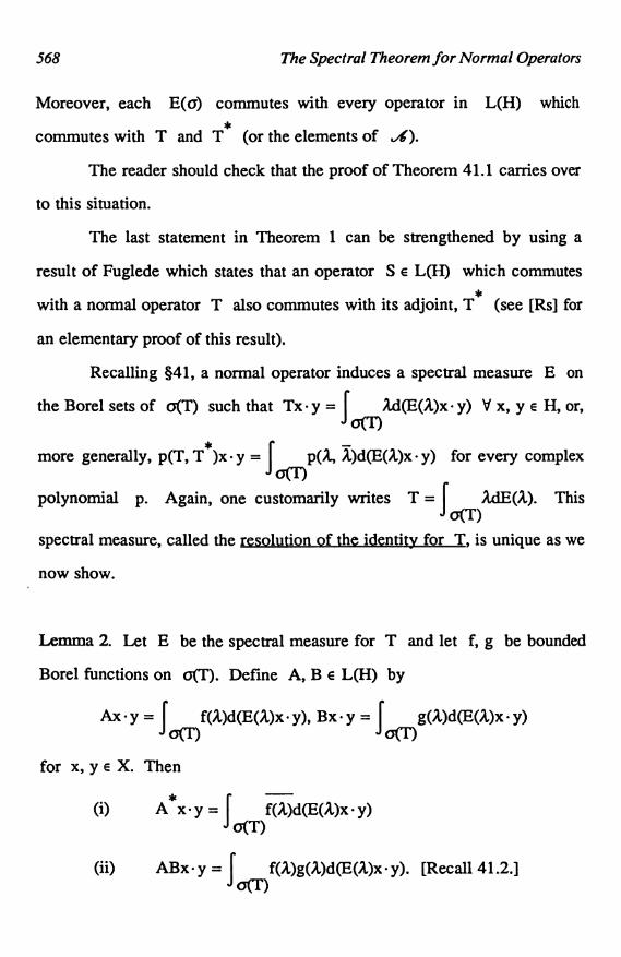
568 The Spectral Theorem for Normal Operators

Moreover, each E(a) commutes with every operator in L(H) which

commutes with T and T (or the elements of ,A).

The reader should check that the proof of Theorem 41.1 carries over

to this situation.

The last statement in Theorem 1 can be strengthened by using a

result of Fuglede which states that an operator S e L(H) which commutes

with a normal operator T also commutes with its adjoint, T (see [Rs] for

an elementary proof of this result).

Recalling §41, a normal operator induces a spectral measure E on

the Borel sets of o(T) such that Tx y = Jo(T)

2.d(E(),)x y) V x, y e H, or,

more generally, p(T,T*)x

y = p(X, X)d(E(X)x y) for every complex

polynomial p. Again, one customarily writes T = Jo(T)

A,dE(X). This

spectral measure, called the resolution of the identity for T, is unique as we

now show.

Lemma 2. Let E be the spectral measure for T and let f, g be bounded

Borel functions on a(T). Define A, B e L(H) by

Ax - y =J O)f

(.)d(E(.X)x y), Bx y =J OMg(2)d(E(.)x

y)

for x, y e X. Then

(i) A*x y = f f(A.)d(E(A)x y)o(T)

(ii) ABx y = f f(,X)g(,,)d(E(A.)x y). [Recall 41.2.]o(T)

Chapter 45 569

We leave the proof to the reader who should consult 41.2.

Corollary 3. The resolution of the identity for T is unique.

Proof: Let F be another resolution of the identity for T. By

Lemma 2,

amp(A, 2)dF(2.) = fO(,1,)p(., A)dE(,X) = Spp(T, T*) = jam p(A,

for every complex polynomial p. By the Stone-Weierstrass Theorem

Six. y =J GMf

(2.)d(E(X)x y) =J OMf

(L)d(F(L)x y)

dfE C(o(T)),x,yE H.

Therefore E(6) = F(6) V 6 e ,$.

Let B(a(T), 2) = B be all the bounded .-measurable, C-valued

functions defined on 0(T). Then B is aB*-algebra

under the involution

f = f. For f E B define an operator f(T) E L(H) by

f(T)x y =J a(T)

f(,I)d(E(2.)x y)

as in Lemma 2 (see Exercise 1). The map f -+ f(T) from B into L(H) is

a norm decreasing *-homomorphism which extends the inverse of the

Gelfand map, f -> Sf (Exercise 5). This map extends the operational

calculus for Hermitian operators which was constructed in §41.

The spectral theorem for normal operators can also be obtained

570 The Spectral Theorem for Normal Operators

directly from the spectral theorem for Hermitian operators. If T e L(H) is

normal, then T has a unique representation as T = A + iB, where A and

B are Hermitian and commute (35.15 and Exercise 35.8). Let E (F) be

the spectral resolution for A (B). Then A = B = and

I = JdE(,X) = jdF(I2). Formally, this gives

T = A + iB = JdE(A)JdF(p) + i fdE(X)J µdF(µ) = ff(A. + ilu)dE(?)dF(µ).

This formal computation suggests that a resolution of the identity for T

can be constructed by constructing a product measure from E and F.

This construction is carried out in [Be]; see also [RN] where a similar

construction using Riemann-Stieltjes integrals is carried out.

There is another version of the spectral theorem for normal

operators which essentially asserts that any normal operator is just

(isomorphic to) a multiplication operator as in Exercise 34.1. For this result

see [TL] V11.7.4 or [DS2].

There are also versions of the spectral theorem for unbounded

operators. These versions of the spectral theorem have applications to

differential operators and quantum theory. For expositions of these versions

of the spectral theorem see [DS2], [RN] or [Cl].

For an interesting historical account of the history of spectral theory,

see [St].

Exercise 1. Show the formulas in Lemma 2 define linear operators A,

B e L(H).

The Spectral Theorem for Normal Operators 571

Exercise 2. Let T E L(H) be normal. Show that T is unitary (Exercise

35.13) if and only if o(T) c { z E C : I z = 11.

Exercise 3. Let T E L(H) be normal with resolution of the identity E.

Show that 2, E o(T) is an eigenvalue if and only if E({),}) * 0.

Exercise 4. Let T E L(H) be normal. Show T is a projection if and only

if o(T) c (0, 1).

Exercise 5. Show the map f -4f(T) is a norm-reducing, *-homomorphism

from B(o(T), 2) to L(H) and JJf(T)xJJ 2 =J OM

I f(,,) 2d(E(A))x x)

Notation

3 TVS 24 38(D)3 F 24 Ck[a, b]5 bal(S) 24 O10 w(,9) k15 QNLS 25 (S2)16 semi-NLS 26 IRn16 NLS17 B-space 26

cn

20 s 26 ba(E)

20 10026 ca(X)

20 c26 var(v) v27 B(S E)

21 c,

0 27 e3o(E)21

c0043 ker T43 AT)

21,22 £ 43 A (T)22 m0 45 L(X, Y)

45 L(X)22 B(S)47 X'22 C(S)

051 rca(S)

22 L (µ)81

Ax

23 Lp(µ) 81 X''" 81 (=ni23 L (µ) xp 91 UBP23 (1)L

105 f(x )23 A [a, b] ,

573

574 Notation

120 cn(f) 318 Al, BI120 sn(f) 347 41(S2)

120 Dn

354 DaT125 (X, Y) 367 W,.P(.Q)140 G(f) 371 spt(f)140 .O (F) 372 spt(T)158 coA 387 K(X, Y)159 abcoA 387 PC(X, Y)

408 W U C160 coA . . .424 W(X Y)

161 PK,

169 o(X, P), LCS 432 t,(X)

181 Ml 432 is (X)

189 X# 432 .4 eY(X, Y)190 a(X, Y) 443 a(T)232 T 443 p(T)

.4237 T(X, X') 445 RA(T)

241 X(E, E') 448 r(T)243 (3(X', X) 451 Pa(T)246 J 451 Ca(T)251 f3*(E, E') 451 Ro(T)

256 Xx 466 T471 m(A)

264 Tb 471 M(A)268 ind(Ea, Aa) 495 HS(H1, H2)

276 Prol(Ea, Aa) 512 P1 1. P2

279 Pq A(T) -,528 IT279 L a (X, Y)535 a(x)

280 (X, Y)L 535 r(x)s535 p(x)

280 LPC(X, Y) 535 RX(x)280 LC(X, Y) 548 rad(X)280 Lb(X, Y) 557 x*

306 Ira 564 (3(S)

310 T'

Appendix: Hilbert Space

In this appendix we set down the basic properties of Hilbert spaces

for those readers not familiar with Hilbert space.


Definition 1. An inner product (scalar product. dot product) on X is a

function : X x X --4 F, (x, y) -4 x y, satisfying

(i) dx,y,ZEX,

(ii) A.(X y) = (Ax) y V X. Y E X, A E F,

(iii) y E X,

(iv) X

(v) x x = 0 if and only if x = 0.

A vector space X with an inner product defined on it is called an

inner product space.

It follows easily from the axioms that 0 x = X-0 = 0,

575

576 Appendix: Hilbert Space

x (Ay) = A(x y) and x (y + z) = x y + x z. We have the important

inequality.

Theorem 2 (Schwarz Inequality). If X is an inner product space, then

(1) S d X, y E X.

Proof: If y = 0, the result is trivial so assume y * 0. In this case,

(1) is equivalent to I x y/ I <_ x x so we may assume y y = 1.

Then

(2) 0:5 (x - (x . Y)Y) (x - (x Y)Y)

= (X-y -Y)

Ix-YI2-(X.Y)(3)-

Remark 3. Equality holds in (1) if x and y are linearly dependent. The

converse also holds for if equality holds in (1) with y * 0, then (2) implies

that x - 0. Note that axiom (v) was not used in the proof of (1).

Proposition 4. If X is an inner product space, the map x - x- x = 11xI1

defines a norm on X.

Proof: Only the triangle inequality needs to be checked. For x,

Y E X,

lix+Y112 = II4 2+ 11y112+x-y+y-x

11X112+ IIYII2+211xIIIlYII =(IIxII + IIYII)2

Appendix: Hilbert Space 577

by Theorem 2.

If X is an inner product space, we always assume that X is

equipped with the norm induced by the inner product.

Proposition 5. The inner product is a continuous function from X x X -4F.

Proof: If xk -4.x and Yk - y, then

Ixkyk - xY1 <_ 1xkyk - xkyI + lxk'Y - x'Yl

s Ilxkll IIYk - YII + Ilxk - 411Y11

by the Schwarz Inequality.

We have the following important property of the norm in an inner

product space.

Proposition 6 (Parallelogram Law). If X is an inner product space, then

IIx+Y112+ I1x-Y112=211x112+211Y112 Vx,yE X.

Proof:

IIx+Y112+ IIx-Y112=(x+y)(x+Y)+(x-Y)'(x-y)=211x112

+211Y112+xy+yx-x.y-yx.

Remark 7. The parallelogram law characterizes inner product spaces

among the class of NLS. That is, if X is a NLS whose norm satisfies the


parallelogram law, then the norm of X is induced by an inner product. If

X is real, the inner product is defined by 4x - y = I1 x + y 112 - lix - y2,

while if X is complex, the inner product is defined by

4x-y= IIx±y112- lix-y112+illx+iyll2-illx-iy112

We leave the (tedious!) verification to the reader.

Definition 8. An inner product space which is complete under the induced

norm is called a Hilbert space.

Example 9. !Rn or Cn is a Hilbert space under the usual inner productn

x y = xiyi' x = (x1' "'' xn)' y = (y1, -I yn)' The norm induced by thei=1

inner product is the Euclidean norm.

Example 10. 12 under the inner product x y = xiyi, x = (xi) ,

i=1

y = Iyi), is a (the original!) Hilbert space.

Example 11. If (S, E, µ) is a measure space, then L2(µ) is a Hilbert

space with the inner product f g = Jfid.

bExample 12. C[a, b] with the inner product f g = f f(t)g(t)dt is an inner

a

product space which is not a Hilbert space.

We establish an important geometric property of Hilbert space.

Theorem 13. Let K be a non-void, closed, convex subset of a Hilbert

space H. If x E H, then there is a unique y E K such that

IIx-Y11=min(IIx-zil : z E K) = dist(x, K).

Furthermore, y can be characterized by:

(3) y e K, A(x - y) (z - y) 5 0 for all z E K.

Proof: Set d = dist(x, K) >_ 0. If w, z E K, applying the

parallelogram law to (x - z)/2 and (x - w)/2 gives

(4) d2<_ II(w+z)/2-x112= 11w-x112/2+IIz-x112/2- II(w-z)/2112

since (w + z)/2 E K.

If IIz - x11 = d and 11w - x11 = d, then (4) implies that w = z so

uniqueness holds.

Pick {yk) c K such that lix - yk11 -+ d. Set w = yk, z = yj in (4)

to obtain

II(Yk-YY)/2II2.:

IIYk-x112/2+IIYj -x112/2-d2_4 0.

Thus, (yk) is a Cauchy sequence in H and converges to some y E K

with lix - YII = d.

If Y E K satisfies Ily - xii = d, then for z r= K and 0 < t < 1,

IIx-yllsllx-tz-(1-t)Y11=IIx-Y-t(z-Y)II

so

Ilx-yll2-or

25 tllz-yII2.

Letting t - 0 gives (3).

On the other hand if y satisfies (3) and z e K,

Ilx-y112- llx-2112=25 liz-y112s0

so llx - yll=d.

Let PK : H -4H be the "projection" map which sends x to y in

Theorem 13. If H = (R2, inequality (3) means that the vector from x to

Pkx makes an obtuse angle with the vector from z to PKx. Moreover,

this map is uniformly continuous on H since IIPKu - PKvll <_ Ilu - vil

[From (3), A (u - PKu) (PKv - PKu) 5 0 and

A (v - PKv) (PKu - PKv) S 0

so adding gives 52 (u - v - (PKu - PKv)) - (PKv - PKu) 5 0 so

IIPKu - PKv l l2 S 52 (u - v). (PKv - PKu) S I l u - V I I I I PKu - PKu l l

by the Schwarz Inequality.]

If X is an inner product space, then two elements x, y e X are

orthogonal, written x y, if x - y = 0. A subset E c X is said to be

orthogonal if x y b x, y r: E, x # y. If E c X is orthogonal and

llxll = 1 V x E E, then E is said to be orthonormal.

2Example 14. In l, (ek : k E [N) is orthonormal.


Example 15. In L2[-7r, 7r], (eint/ : n = 0, ± 1, ... ) is orthonormal.

Proposition 16 (Pythagorean Theorem ). If x 1 y, then

l1x+Y112=lix-Y112=II4 2+IIYII2.

Proof: (x+y).(x+y)= 11x+Y112=11x112+ IIYII2=(x-y).(x-y).

If X is an inner product space and M c X, we set

M1=(xeX:xly dyEM);

Ml is called the orthogonal complement of M. Note that M1 is a closed

linear subspace of X. We now use Theorem 13 to show that any closed

linear subspace of a Hilbert space is complemented.

Theorem 17. If M is a closed linear subspace of a Hilbert space H, then

H=M®M1.

Proof: For x e H let y = PMx e M be as in Theorem 13. Then

x - y e M1 since by (3) A (x - y) w S 0 for every w E M.

Hence, x = (x - y) + y with x - y E M1 and y e M. Since

MnM1= (0),wehave H=M9Ml.

Thus, every closed linear subspace of a Hilbert space has a

projection onto it. This property actually characterizes Hilbert spaces

among the class of B-spaces ([LT]).

We can now establish the Riesz Representation Theorem for filbert

space.

Proposition 18. Let H be a Hilbert space and y E H. If fy : H -4F is

defined by y, x> = then fy E H' and 11f II = Ilyll.

Proof: f is clearly linear and since I <fy, x> I = I x. y I s Ilxll IIYII

yEH' with IIYII_ Ilyll. Since y,y>=y-y=IIYII2,IIyII=IIYII.

Thus, the map y - f is an isometry from H into its dual space

H'. We show that this map is onto.

Theorem 19 (Riesz Representation Theorem). If H is a Hilbert space and

f E H', then 3 a unique y E H such that f = y.

Proof: If f = 0, put y = 0. Suppose f ;e 0. Set M = ,K(f) so M

is a proper closed subspace of H and Ml * (0). Choose Z E Ml, z : 0.

Then <f, z> # 0. Set y = (<F,-i>/IIzII2)z SO y E Ml, y 0, and

<f, Y> = I <f, z> 12/112112 = y y. For x E H, let x1 = x - (<f, x>/IIy112)Y.

x2 = (<f, x>/IIY112)y so x = x1 + x2 and <f, x1>=O so x1 E M and

x1 y = 0. Hence, x y = x2 y = <f, x> = y, x>, and f = y.

The map 1 : y -a f is an isometry from H onto H' which is

additive but is only conjugate homogeneous in the sense that

D(ty) = ic(y). From this it follows that Hilbert spaces are always reflexive.

If X is an inner product space and E = (xa :a E A) is ann

orthonormal subset of X, then d x r= X the scalars x(a) = x - xa, a E A, are


called the Fourier coefficients of x with respect to E. We establish

several important properties of the Fourier coefficients.

Proposition 20. Let X be an inner product space and (x1, ..., xn) an

orthonormal set in X. Then for each x E X,n n

(1)Ix.xil2= Ix(1)I2 llx,12,

i=1n

i=1

(ii) (x - (x xi)xi) xi Vi.i=1

Proof: (i):n n n

05 jjx - (x' xi)xiII2 = (x - (x xi)xi, x - (x xi)xi)i=1 i=1 i=1

_ IIxII2 - (x xi)(x - xi) - (x xi (x xi)i i

+ (x. xi)(x xi J = 11xII2 -ij i

(ii): (x - (x -Xi)Xi, xj) = x l - (x . xi)(xi xj ) = x xj - x i = 0.

i i

We generalize the inequality in (i) to infinite orthonormal sets.

Proposition 21. Let E = {xa a E A) be an orthonormal set in an inner

product space X. For each x E X the set Ex = (a e A : x xa : 0) is at

most countable.

584

Proof: For

Proposition 20 Sn

the result follows.

Appendix: Hilbert Space

n e IN, let Sn = {a E A : jjxjj2/n}. By

00

contains at most n - 1 elements. Since Ex = v Sn,n=1

Theorem 22 (Bessel's Inequality). Let E = (xa : a e A) be an orthonormal

subset of an inner product space X. For each x E X,

(5)Ix-xal2

=Ix(a)I2

5 IIxIi2.aEA aeA

Proof: If A is finite, this is Proposition 20. If A is infinite, we

must assign a meaning to the series in (5). Let S = {a E A : 0}. If

S = 0, we set I x xa l 2 = 0, and if S is finite, we setaE A

Z Ixxal2 = C Ix.xal2

aEA aES

and (5) follows from Proposition 20. If S is infinite, S is countable by

Proposition 21 so the elements (xa : a e S) can be arranged in a sequence,

say y1, y2, .... By Proposition 20, d nn

z 5 IIxII2

i=1

00

so the series I x yi 12 is absolutely convergent and its sum isi=1

independent of the ordering of the elements (xa a E S). Therefore, we


may defineI

IjxII2 by

aEA i=1 aEA

Proposition 20.

We will now show that equality holds in Bessel's Inequality for

certain orthonormal sets in a Hilbert space. An orthonormal subset E of a

Hilbert space H is said to be complete (or a complete orthonormal set) if

El c H orthonormal and E1 ? E implies that E = E1 (i.e., E is a

maximal orthonormal set with respect to set inclusion). We give several

criteria for an orthonormal set to be complete. First, we require a lemma.

Lemma 23. Let {xl, ..., xn} be an orthonormal set in an inner product

space X.

(i) If thenn

ck = x xk = x(k) and

k=1n

(ii) For {c1, ..., cn} c F, lix - ckxkll attains its minimumk=1

A(as a function of (c1, ..., cn)) at ck = x xk = x(k),

k = 1, ..., n.

Proof: (i): That ck = x xk is immediate;

Cn

=Lckcjxk _ Icki 2Ik j k=1

n n n

0< 11x - ckxk112 = (x - I ckxk) (x - ckxk)k=1 k=1 k=1

n n n

= 11 x 112 ck(x' xk - ck(x ' xk) + 1 ck 12

k=1 k=1 k=1

n n

_ (11x112 - Ix'xk12) + Ck

k=1 k=1

and the expression on the right is clearly minimal at Ck = x xk.

Theorem 24. Let E = (xa : a E A) be an orthonormal set in a filbert

space H. The following are equivalent:

(i) E is complete,

(ii) X ,. Xa d a E A implies x= 0,

(iii) span E is dense in H

(iv) If x E H, 11x112 = 1 x xa 12 (equality in Bessel's

aE A

Inequality)

(v) x = (x xa)xa V x E H,aEA

(vi) if x, y E H, x y = (x xa)(y (Parseval's Equality).aaE A

Proof: (i) * (ii): If (ii) is false, 3 x # 0 such that x 1 xa b a E A.

Set z = x/IIxlI so {z) v E is an orthonormal set which properly contains

E so (i) does not hold.

(ii) (iii): Let M be the closure of span E. If M t- H,

H=M®M1 with M'* {0}. If x* 0,xEMl,then xlxa VaEA so(ii) fails.

(iii) * (iv): Let e > 0 and x E H. 3 xa , ..., xa E E and1 n

n

c1, ..., cn r= F such that llx - ckxa II < e. By Lemma 23 (ii),k=1

k

n

(6) lix - (x xa )xa II < Ek=1

By Lemma 23 (i) and (6),

n n

(IIXII - E) 2 < II Ix.xakI2 Ix.xaI2k=1 k=1 aEA

Bessel's Inequality gives the reverse inequality.

(iv) * (v): As in Theorem 22 let S = (xa : xa x # 0) and arrange

the elements of S into a sequence yl, y27 .... Then

n n

lix - ZIlxll2 _ z

Ix.ykl2

k=1 k=100 n CO

_Ix

ykl2_ Ix.yk12 =L

Ix.ykl2

k=1 k=1 k=n+1

CO

by (iv). Hence, x = (x yk)yk = ' (x xa)xa.k=1 aEA

(v) * (vi): By Proposition 5,

x y = C (x xa)(y xb)xa xb = (x ' xa)( xaaEA bEA aEA


(vi) * (i): If (i) fails, 3 z E H with Ikzil = 1 and z i xa d a E A.

Then z - z = 1 while I z - xa 1 2 = 0 so (vi) fails.aE A

Theorem 25. Let H be a Hilbert space with E and F complete

orthonormal subsets. Then E and F have the same cardinality.

Proof: Since orthonormal sets are linearly independent, we may

assume that E and F are infinite.

For e E E, let Fe = If E F : f - e *0). By Theorem 24 (ii),

F= u Fe and by Proposition 21 each Fe is at most countable. Hence,eEE

the cardinality of F is less than or equal to the cardinality of E.

Symmetry gives the reverse inequality.

The cardinality of a (any) complete orthonormal set is called the

orthonormal dimension of the Hilbert-space.

Example 26. {ek : k E a} is a complete orthonormal subset of I2

Example 27. (eint14-T z-: n = 0, ± 1, ...) is a complete orthonormal subset

of L2[-7r, 7G] ([HS] IV.16.32).

Exercise 1. Show that any orthonormal subset of a Hilbert space is

contained in a complete orthonormal set.


Exercise 2. Show a Hilbert space is separable if and only if its orthonormal

dimension is countable.

Exercise 3. In Theorem 24, the map x - ( x xa : a E A) is an isometry

from H into a 2(A). Show this map is onto (this is the Riesz-Fischer

Theorem). Thus, any Hilbert space is isomorphic to some Q 2(A).

Exercise 4. If D is a dense subset of an inner product space and x 1. D,

show x = 0.

Exercise 5. If E is a linear subspace of a Hilbert space H, Y is a

B-space and T : E -4Y is a continuous linear operator, show T has an

continuous linear extension T : H -4Y. [Compare with the remark

following 27.5.]

Exercise 6 (Gram-Schmidt). Let x1, ..., xn be linearly independent. Set

kcc-1

y 1 = xl' yk = Xk - G(xk yj)yj for k > 1 and zk = Yk/IIYkil Show

j=1{zk} is orthonormal and span( xk) = span {zk}.

References

[Ag] S. Agmon, Elliptic Boundary Value Problems, Van Nostrand,Princeton, 1965.

[AB] C. Aliprantis and O. Burkinshaw, Principles of Real Analysis,Academic Press, N.Y., 1990.

[A] P. Antosik, On uniform boundedness of families of mappings,Proc. Conf. Conv. Structures, Szczyrk, 1979, 2-16.

[AS] P. Antosik and C. Swartz, Matrix Methods in Analysis,Springer-Verlag, Heidelberg, 1985.

[BN] G. Bachman and L. Narici, Functional Analysis, Academic Press,N.Y., 1966.

[B] S. Banach, Oeuvres II, Acad. Pol. Sci., Warsaw, 1979.[BK] G. Bennett and N. Kalton, FK-Spaces Containing c0, Duke Math.

J., 39 (1972), 561-582.[Be] S. Berberian, Notes on Spectral Theory, Van Nostrand, Princeton,

1966.[Bo] N. Bourbaki, Topological Vector Spaces, Springer-Verlag, Berlin,

1987.[BM] J. Burzyk and P. Mikusiuski, On normability of semigroups, Bull.

Acad. Polon. Sci., 28 (1980), 33-35.[BKL] J. Burzyk, C. Klis and Z. Lipecki, On metrizable Abelian groups

with a completeness-type property, Colloq. Math., 49 (1984),33-39.

[Co] J. Connor, A Short Proof of Steinhaus' Theorem on Summability,Amer. Math. Monthly, 92 (1985), 420-421.

[Cl] J. Conway, A Course in Functional Analysis, Springer-Verlag,N.Y., 1985.

[C2] J. Conway, The Inadequacy of Sequences, Amer. Math. Monthly,76 (1969), 68.

591

592 References

[C3] J. Conway, The Compact Operators are not Complemented inB(H), Proc. AMS, 32 (1982), 549-550.

[Da] M. Day, Normed Linear Spaces, Springer-Verlag, N.Y., 1962.[DeS] J. DePree and C. Swartz, Introduction to Real Analysis, Wiley,

N.Y., 1987.[DU] J. Diestel and J. Uhl, Vector Measures, Amer. Math. Soc. Surveys

#15, Providence, 1977.[Dr] L. Drewnowski, Equivalence of Brooks-Jewett, Vitali-Hahn-Saks

and Nikodym Theorems, Bull. Pol. Acad. Sci., 20 (1972),725-731.

[DS] N. Dunford and J. Schwartz, Linear Operators I, Interscience,N.Y., 1953.

[DS2] N. Dunford and J. Schwartz, Linear Operators II, Interscience,N.Y. 1963.

[El] P. Enflo, A counterexample to the approximation problem inBanach spaces, Acta Math., 130 (1973), 309-317.

[E2] E. Enflo, On the invariant subspace problem for Banach spaces,Acta Math., 158 (1987), 213-313.

[FW] K. Floret and J. Wloka, Einfiihrung in die Theorie lokalkonvexerRaume, Lecture Notes in Math. 56, Springer-Verlag, Heidelberg,1968.

[Fr] J. Franklin, Methods of Mathematical Economics,Springer-Verlag, N.Y., 1980.

[GS] I. M. Gelfand and G. E. Shilov, Generalized Functions, AcademicPress, N.Y., 1964.

[Gol] S. Goldberg, Unbounded Linear Operators, McGraw-Hill, N.Y.,1966.

[Go2] S. Goldberg, Some Properties of the Space of compact Operatorson a Hilbert Space, Math. Ann., 138 (1959), 329-331.

[Gr] A. Grothendieck, Topological Vector Spaces, Gordan and Breach,N.Y., 1973.

[Ha] H. Hahn, Uber Folgen linearen Operationen, Monatsch. fur Mathand Phys., 32 (1922), 1-88.

[HT] E. Hellinger and O. Toeplitz, Grundlagen fur eine Theorie derunendlichen Matrizen, Math. Ann., 69 (1910), 289-330.

[HL] H. Hermes and J. P. LaSalle, Functional Analysis and TimeOptional Control, Academic Press, N.Y., 1969.

[HS] E. Hewitt and K. Stromberg, Real and Abstract Analysis,Springer-Verlag, N.Y., 1965.

[Hi] T. H. Hildebrandt, Integration in Abstract Spaces, Bull. Amer.Math. Soc., 59 (1953), 111-139.

[HP] E. Hille and R. Phillips, Functional Analysis and Semi-Groups,Amer. Math. Soc., Providence, 1957.

[Ho] H. Hochstadt, Eduard Helly, Father of the Hahn-BanachTheorem, Math. Intell., 2 (1979), 123-125.

[H1] J. Horvath, Topological Vector Spaces and Distributions,Addison-Wesley, Reading, 1966.

[H2] J. Horvath, An Introduction to Distributions, Amer. Math.Monthly, 77 (1970), 227-240.

References 593

[J1] R. C. James, A non-reflexive Banach space isometric with itssecond conjugate space, Proc. Nat. Acad. Sci. USA, 37 (1951),174-177.

[J2] R. C. James, Reflexivity and the sup of linear functionals, IsraelJ. Math., 13 (1972), 289-300.

[J3] R. C. James, Bases in Banach Spaces, Amer. Math. Monthly 82(1989), 625-640.

[Jo] J. Johnson, Remarks on Banach Spaces of Compact Operators, J.Functional Anal., 32 (1979), 304-311.

[Jor] O. G. Jorsboe, Set Transformations and Invariant Measures,Aarhus Universitet, 1966.

[Ke] J. Kelley, General Topology, Van Nostrand, Princeton, 1955.[Kl] C. Klis, An Example of noncomplete normed (K)-space, Bull.

Pol. Acad. Sci., 26 (1978), 415-420.[K] A. Kolmogorov, Zur Normierbarkeit eines allgemeinen

topologischen linearen Raumes, Studia Math., 5 (1934), 29-33.[Kom] Y. Komura, Some examples on linear topological spaces, Math.

Ann., 153 (1964), 150-162.[K1] G. KSthe, Topological Vector Spaces I, Springer-Verlag, N.Y.,

1969.[K2] G. Kothe, Topological Vector Spaces II, Springer-Verlag, N.Y.,

1979.[LL] I. Labuda and Z. Lipecki, On subseries convergent series and

m-quasi-bases in topological linear spaces, Manuscripta Math., 38(1982), 87-98.

[LT] J. Lindenstrauss and L. Tzafriri, Classical Banach Spaces I,Springer-Verlag, N.Y., 1977.

[L] J. Liitzen, The Prehistory of the theory of distributions,Springer-Verlag, N.Y., 1982.

[Ma] I. Maddox, Infinite Matrices of Operators, Springer-Verlag,Heidelberg, 1980.

[MO] S. Mazur and W. Orlicz, Uber Folgen linearen Operationen,Studia Math., 4 (1933), 152-157.

[Me] M. D. Meyerson, Every power series is a Taylor series, Amer.Math. Monthly, 88 (1981), 51-52.

[M] M. Munroe, Introduction to Measure and Integration,Addison-Wesley, Reading, Mass., 1953.

[NB] L. Narici and E. Beckenstein, Topological Vector Spaces, MarcelDekker, N.Y., 1985.

[NS] A. W. Naylor and G. R. Sell, Linear Operator Theory,Holt-Rinehart-Winston, N.Y., 1971.

[vN] J. von Neumann, On complete topological spaces, Trans. Amer.Math. Soc., 37 (1935), 1-20.

[P] E. Pap, Functional analysis with K-convergence, Proceedings ofConference on Convergence Spaces, Bechyne, Czech. 1984,Akademie-Verlag, 245-250.

[PS] E. Pap and C. Swartz, Pap's Adjoint Theorem in Locally ConvexSpaces.

[Ph] R. Phillips, On Linear Transformations, Trans. Amer. Math. Soc.,

594 References

48 (1940), 516-541.[Pi] A. Pietsch, Quasi-nukleare Abbildungen in normierten Raumen,

Math. Ann., 165 (1966), 76-90.[Ri] N. M. Rice, On nth Roots of Positive Operators, Amer. Math.

Monthly, 89 (1982), 313-314.[RN] F. Riesz and B. Nagy, Functional Analysis, Unger, N.Y., 1955.[RR] W. Robertson and A. Robertson, Topological Vector Spaces,

Cambridge University Press, Cambridge, 1964.[Rs] M. Rosenblum, On a Theorem of Fuglede and Putnam, J. London

Math. Soc., 33 (1958), 376-377.[Ro] R. L. Royden, Real Analysis, MacMillan, N.Y., 1988.[Rul] W. Rudin, Real and Complex Analysis, McGraw-Hill, N.Y.,

1966.[Ru2] W. Rudin, Functional Analysis, McGraw-Hill, N.Y., 1973.[S] W. L. C. Sargent, On Some Theorems of Hahn, Banach and

Steinhaus, J. London M. S., 28 (1953), 438-451.[Sa] S. Saxon, Some normed barrelled spaces which are not Baire,

Math. Ann., 209 (1974), 153-160.[Sc] J. Schur, Uber lineare Transformation in der Theorie die

unendlichen Reihen, J. Reine Angew. Math., 151 (1920), 79-111.[Sch] L. Schwartz, Theorie des Distributions I, II, Hermann, Paris,

1951.[Sm] G. Simmons, Introduction ' to Topology and Modem Analysis,

McGraw-Hill, N.Y., 1963.[Si] I. Singer, Bases in Banach Spaces I, Springer-Verlag, N.Y., 1970.[St] L. Steen, Highlights in the History of Spectral Theory, Amer.

Math. Monthly, 80 (1973), 359-381.[Sw] C. Swartz, The Evolution of the Uniform Boundedness Principle,

Math. Chron., 19 (1990), 1-18.[Sz] Szankowski, B(H) does not have the approximation property,

Acta Math., 147 (1981), 89-108.[Ta] A. Taylor, Notes on the History and Uses of Analyticity in

Operator Theory, Amer. Math. Monthly, 78 (1971), 331-342.[TL] A. Taylor and D. Lay, Introduction to Functional Analysis,

Wiley, N.Y., 1980.[Ti] F. Treves, Topological Vector Spaces, Distributions and Kernels,

Academic Press, N.Y., 1967.[T2] F. Treves, Applications of Distributions to PDE Theory, Amer.

Math. Monthly, 77 (1970), 227-240.[T3] F. Treves, Basic Linear Partial Differential Equations, Academic

Press, N.Y., 1975.[V] M. Valdivia, Br complete spaces which are not B-complete,

Math. Zeit. 185 (1984), 253-259.[Whl] R. Whitley, An Elementary Proof of the Eberlein-Smulian

Theorem, Math. Ann., 172 (1967), 116-118.[Wh2] R. Whitley, Projecting m onto co, Amer. Math. Monthly, 73

(1966), 285-286.

References 595

[Wh3] R. Whitley, The Spectral Theorem for a Normal Operator, Amer.Math. Monthly, 75 (1968), 856-861.

[W] A. Wilansky, Modern Methods in Topological Vector Spaces,McGraw-Hill, N.Y., 1978.

[Y] K. Yosida, Functional Analysis, Springer-Verlag, Berlin, 1966.

Index

.A-space, 41absolutely convergent, 18absolutely convex, 158absolutely convex hull, 159absolutely summing, 431absolutely summing norm, 433absorbs, absorbed, 7adjoint, 466almost open, 137, 303almost separable valued, 339a-dual, 256analytic, 123annihilator, 63, 318approximate eigenvalue, 453, 478approximate point spectrum, 453Approximation Property, 393

B-algebra, 559*

B -algebra, 559B-complete, 330Br complete, 330

*B -subalgebra, 559Baire space, 296balanced, 4balanced hull, 5

Banach algebra, 533Banach limit, 86Banach-Mackey space, 253Banach space (B-space), 17barrel, 245, 295barrelled LCS, 295bidual, 81, 246bilinear, 105Bochner integral, 340bomivore, 245, 261bornivorous, 245bornological, 261bornological topology, 264bounded (set), 37bounded (map), 44bounded multiplier convergent, 417bounded self adjoint, 473bounds, 471

C -algebra, 559canonical map (imbedding), 81, 246Cauchy net, 11Cauchy principal value, 353Cauchy sequence, 175closed convex hull, 160closed mapping, 140coercive, 366

597

598

compact (operator), 387compatible, 192, 237complementary, 382complete, 11completely continuous,'397completion, 178condensation of singularities, 121conditionally countably compact, 222conditionally sequentially compact, 223continuous spectrum, 451convex, 157

convex combination, 157convex hull, 158coordinate functionals, 146countably valued, 338

derivative (distributional), 354distribution, 347dual, 47dual norm, 47duality, 189

eigenvalue, 451.eigenvector, 451equicontinuous, 53, 109

left (right), 108extremal point, 184extremal subset, 184extreme point, 184

F-space, 35finite order, 350Frechet quasi-norm, 14Fredholm integral operator, 286fully complete, 330

gauge, 161

Gelfand integral, 334map, 520representation, 547topology, 547transform, 547

generalized functions, 352Generalized Schwarz Inequality, 480graph, 140Green's function, 504

Heaviside function, 355Hermitian, 473, 557

Index

Hilbert-Schmidt operator, 494Hilbert space adjoin[, 466*-homomorphism, 560hyperplane, 166hypocontinuous, 107, 300

ideal, 545inductive limit topology, 268infinite nuclear, 413infra-barrelled, 249infra-Ptak, 330invariant, 461invertible, 282, 534involution, 557isometry, 47*-isomorphism, 560

,X-bounded, 40X convergent, 19X matrix, 94i i' space, 19kernel, 286, 287

LB-space, 270LF-space, 270left shift, 55linear functional, 47linearly isometric, 47linked, 219locally convex topology, 169locally convex TVS (LCS), 169locally finite, 359locally null, 15

Mackey convergent, 15space, 240topology, 232, 237

maximal ideal space, 548metric linear space, 34metrically bounded, 39metrizability

space, 33unit ball, 213

Minkowski functional, 161moment problem, 89Montel (space), 349

Neumann series, 283non-atomic, 204

Index

norm, 16normal, 246, 476, 557normable, 182nonmed linear space (NLS), 16norming set, 80nuclear (bilinear form), 180

operational calculus, 527operator norm, 46operator, 45order, 350orthogonal projection, 509

partition of unity, 360perfect, 256perpendicular, 512Pettis integral, 334point spectrum, 451polar, 199polar topology, 232precompact, 177precompact operator, 387predual, 204projection, 381, 542projective limit, 276pseudo function, 353Ptak space, 330

quasi-barrelled, 249quasi-complete, 227, 274quasi-norm, 13quasi-nonmed space (QNLS), 15

radical, 548rapidly decreasing functions, 365reciprocal kernel, 287reflexive, 81, 247regular inductive limit, 272

summability method, 125relatively compact, 222residual spectrum, 451resolution of the identity, 526, 568resolvent, 535resolvent equation, 445, 535resolvent operator, 445resolvent set, 443, 535right shift, 55Root Test, 284

599

Sargent space, 102, 103scalarly integrable, 334

measurable, 336Schauder basis, 146Schur space, 216Schwartz distribution, 347second dual, 81semi-metric linear space, 34semi-Montel space, 349semi-norm, 16semi-normed linear space

(semi-NLS), 16semi-reflexive, 247semi-simple, 548separate, 166separately continuous, 105sequentially complete, 11, 176series, 18sesquilinear, 515simple (function), 336singular, 534Sobolev space, 367spectral measure, 525

radius, 448, 535spectrum, 443, 535square root, 528Stone-Cech Compactification, 563strict inductive limit, 270strong operator topology, 281strong topology, 232, 243strongest locally convex

topology, 181strongly continuous semi-group, 529strongly elliptic, 368strongly measurable, 336Sturm-Liouville (operator), 470sublinear functional, 73subseries convergent, 220, 416summability, 125support, 206, 372symmetric, 4, 316, 469, 516

tempered distributions, 365test functions, 347Theorem

Antosik-Mikusinski, 92Banach-Alaoglu, 202Banach-Dieudonne, 292Banach-Mackey, 253

600

Banach-Mazur, 328Banach-Steinhaus, 299Basic Matrix, 92Bessaga-Pelczynski, 411Bipolar, 201Bohnenblust-Sobczyk, 75Borel, 379Closed Graph (CGT), 142, 33Closed Range, 325de Branges, 207Diagonal, 92Drewnowski, 112, 113Dvoretsky-Rogers, 440Fredholm Alternative, 403Gantmacher, 426Gelfand-Mazur, 537General UBP, 95Goldstine, 210Hahn-Banach, 74, 76Hahn-Schur, 127Hellinger-Toeplitz, 133, 258,

316, 473Hilbert-Schmidt, 491Kakutani, 33Kolmogorov, 182Krein-Milman, 186Krein-Smulian, 293Lax-Milgram, 366Liapounoff, 204Lomonosov, 461Mackey-Arens, 239Mackey, 175, 178, 194Mazur-Orlicz, 106Nikodym Boundedness, 112,Nikodym Convergence, 130Open Mapping (OMT), 138,Orlicz-Pettis, 221, 242Pettis, 339Phillips, 216, 383Riesz, 67Schauder, 393Schur, 216Silvermann-Toeplitz, 131Smulian-Eberlein, 226Sobczyk, 384Spectral Mapping, 449, 529

Index

Steinhaus, 133Stone-Weierstrass, 207Terzioglu, 407Uniform Boundedness (UBP),

103, 229, 254, 304Wiener, 553

topological divisor of 0, 536topological vector space (TVS), 3topology of bounded convergence, 280

of pointwise convergence, 28of uniform ,9-convergence,of uniform convergence, 232

total (quasi-norm), 13totally bounded, 177translation invariant, 15transpose, 310triangle inequality, 13

unconditonal Schauder basis, 419unconditionally converging

operator, 438unconditionally convergent, 416uniform norm, 46uniform operator topology, 280uniformly bounded, 94

continuous semi-group, 529countably additive, 130

unitary operator, 484unordered convergent, 417

vanishes, 371vector topology, 3Volterra integral operator, 287

weak solution, 370topology, 190, 192

weak topology, 192weak operator topology, 281weakly compact operator, 423

continuous, 312integrable, 334unconditionally Cauchy

(w.u.c.), 408weight function, 470Wiener algebra, 552

an introduction to functional analysis - sv.20file.orgsv.20file.org/up1/1408_0.pdf · nita ruth....

Documents