an introduction to nonequilibrium many-body theorystafford/courses/560a/nonequilibrium.pdf · an...

Joseph Maciejko

An Introduction toNonequilibrium Many-BodyTheory

October 25, 2007

Springer

Contents

1 Nonequilibrium Perturbation Theory . . . . . . . . . . . . . . . . . . . . . . 11.1 Failure of Conventional Time-Ordered Perturbation Theory . . . 1

1.1.1 Equilibrium Many-Body Theory . . . . . . . . . . . . . . . . . . . . . 11.1.2 Failure of Conventional Techniques . . . . . . . . . . . . . . . . . . 2

1.2 The Schwinger-Keldysh Contour . . . . . . . . . . . . . . . . . . . . . . . . . . . 51.3 The Closed Time Path Contour . . . . . . . . . . . . . . . . . . . . . . . . . . . 71.4 Interactions: the Kadanoff-Baym Contour . . . . . . . . . . . . . . . . . . 8

1.4.1 Neglect of Initial Correlations and Schwinger-KeldyshLimit . . . . . . . . . . . . . . . . . . . . . . . . . . . . . . . . . . . . . . . . . . . . 10

1.5 Contour Dyson Equation . . . . . . . . . . . . . . . . . . . . . . . . . . . . . . . . . 111.6 Initial Correlations with Arbitrary Initial Density Matrix . . . . . 121.7 Relation to Real-Time Green’s Functions . . . . . . . . . . . . . . . . . . . 12

1.7.1 Larkin-Ovchinnikov Representation . . . . . . . . . . . . . . . . . . 131.7.2 Langreth Theorem of Analytic Continuation . . . . . . . . . . 14

2 Quantum Kinetic Equations . . . . . . . . . . . . . . . . . . . . . . . . . . . . . . . 172.1 Keldysh Equation . . . . . . . . . . . . . . . . . . . . . . . . . . . . . . . . . . . . . . . 182.2 Kadanoff-Baym Equation . . . . . . . . . . . . . . . . . . . . . . . . . . . . . . . . . 21

2.2.1 Wigner Representation and Gradient Expansion . . . . . . . 232.3 Quantum Boltzmann Equation . . . . . . . . . . . . . . . . . . . . . . . . . . . . 27

2.3.1 QBE with Electric Field . . . . . . . . . . . . . . . . . . . . . . . . . . . . 272.3.2 QBE with Electric and Magnetic Field . . . . . . . . . . . . . . . 282.3.3 One-Band Spinless Electrons . . . . . . . . . . . . . . . . . . . . . . . . 30

3 Applications . . . . . . . . . . . . . . . . . . . . . . . . . . . . . . . . . . . . . . . . . . . . . . . 333.1 Nonequilibrium Transport through a Quantum Dot . . . . . . . . . . 33

3.1.1 Expression for the Current . . . . . . . . . . . . . . . . . . . . . . . . . 353.1.2 Perturbation Expansion for the Mixed Green’s Function 353.1.3 Path Integral Derivation of the Mixed Green’s Function 373.1.4 General Expression for the Current . . . . . . . . . . . . . . . . . . 393.1.5 Noninteracting Quantum Dot . . . . . . . . . . . . . . . . . . . . . . . 41

VI Contents

3.1.6 Interacting Quantum Dot: Anderson Model andCoulomb Blockade . . . . . . . . . . . . . . . . . . . . . . . . . . . . . . . . . 42

3.2 Linear Response for Steady-State and Homogeneous Systems . 443.2.1 Example: Conductivity from Impurity Scattering . . . . . . 48

3.3 One-Band Electrons with Spin-Orbit Coupling . . . . . . . . . . . . . . 503.4 Classical Boltzmann Limit . . . . . . . . . . . . . . . . . . . . . . . . . . . . . . . . 52

References . . . . . . . . . . . . . . . . . . . . . . . . . . . . . . . . . . . . . . . . . . . . . . . . . . . . . 57

1

Nonequilibrium Perturbation Theory

The goal of this chapter is to construct the perturbation expansion for the1-particle contour-ordered Green’s function. First, we explain why the usualperturbation expansion on the Feynman contour (the real-time axis from −∞to ∞) or on the Matsubara contour (a segment on the imaginary-time axisfrom −iβ to iβ) fails in general nonequilibrium situations.

1.1 Failure of Conventional Time-Ordered PerturbationTheory

The central goal of nonequilibrium many-body theory is to calculate real-timecorrelation functions. For example, we might want to calculate the 1-particletime-ordered Green’s function,

iG(x, t;x′, t′) = 〈T [ψ(x, t)ψ†(x′, t′)]〉 = Tr ρT [ψ(x, t)ψ†(x′, t′)] (1.1)

in the Heisenberg picture, where ρ is an arbitrary nonequilibrium densitymatrix and the Hamiltonian H(t) is in general time-dependent.

1.1.1 Equilibrium Many-Body Theory

In conventional equilibrium many-body theory, we know how to setup a per-turbation theory to calculate this quantity. At zero temperature, the densitymatrix is

ρ = |Ψ0〉〈Ψ0| (1.2)

where |Ψ0〉 is the exact ground state of a full interacting but time-independentHamiltonian H. Then the time-ordered Green’s function

iG(x, t;x′, t′) = 〈Ψ0|T [ψ(x, t)ψ†(x′, t′)]|Ψ0〉 (1.3)

is given by conventional Feynman-Dyson perturbation theory,

2 1 Nonequilibrium Perturbation Theory

iG(x, t;x′, t′) =〈Φ0|T [S(∞,−∞)ψ(x, t)ψ†(x′, t′)]|Φ0〉

〈Φ0|S(∞,−∞)|Φ0〉(1.4)

where the caret denotes operators in the interaction picture with respect toa quadratic Hamiltonian H0 where H = H0 + V , |Φ0〉 is the ground state ofH0, and the S-matrix is

S(∞,−∞) = T exp(−i∫ ∞

−∞dt1 V (t1)

)(1.5)

The power series expansion of the S-matrix and the subsequent use of Wick’stheorem generates the usual Feynman diagrams, of which the disconnectedones cancel against the phase factor in the denominator.

At finite temperatures, we use the coincidence in functional form of thethermal density matrix

ρ =e−βH

Z(1.6)

where Z = Tr e−βH is the partition function, and the evolution operatorU(t) = e−iHt to setup a perturbation theory in imaginary time. Here again,Wick’s theorem can be used since each term in the perturbation expansionis an average over a noninteracting density matrix ρ0 = e−βH0/Z0 whereZ0 = Tr e−βH0 .

1.1.2 Failure of Conventional Techniques

These techniques seem quite powerful, so why can’t we apply them to themore general problem of Eq. (1.1)?

Let us consider the Matsubara technique first. Out of equilibrium, thereis no such thing as a temperature. As a result, in general the density matrixis not of exponential form, so there is no way we can use the Matsubaratrick which consists in a simultaneous expansion of the density matrix andthe time-evolution operator allowed by the coincidence in functional form ofthese two operators.

In the Feynman case, once again the density matrix is not a simple pro-jector on the ground state as in Eq. (1.2).

These arguments are correct, but it is instructive to see in more detailwhere exactly does the mathematical construction of the above equilibriumperturbation expansions fail. We will try to construct an expansion of thenonequilibrium Green’s function using the ordinary Feynman approach andsee that it fails.

Consider a generic density matrix

ρ =∑Φ

pΦ|Φ〉〈Φ| (1.7)

1.1 Failure of Conventional Time-Ordered Perturbation Theory 3

where the |Φ〉 can be arbitrary quantum states. First recall that in the Heisen-berg picture, the density matrix does not evolve in time since its time evolu-tion, given by the quantum Liouville equation, goes in a way opposite to thatgiven by the Heisenberg equation of motion, so that the time evolution of ρcancels out altogether. For convenience, we study one state at a time, namelywe want to calculate the expectation value

iGΦ(x, t;x′, t′) = 〈Φ|T [ψ(x, t)ψ†(x′, t′)]|Φ〉 (1.8)

and we can obtain the full Green’s function by G =∑

Φ pΦGΦ.Now consider the following partition of the Hamiltonian H(t) = H+H ′(t)

where H is the unperturbed equilibrium Hamiltonian (but may still containinteractions) and all the time dependence is included in the nonequilibriumperturbation H ′(t). The field operator in the interaction picture is

ψ(x, t) = eiHtψ(x)e−iHt (1.9)

and in the Heisenberg picture,

ψ(x, t) = U†(t)ψ(x)U(t) = S(0, t)ψ(x, t)S(t, 0) (1.10)

where S(t, 0) = eiHtU(t) and the evolution operator is

U(t) = T exp(−i∫ t

0

dt1H(t1))

(1.11)

more generally, we have the S-matrix

S(t, t′) = eiHtU(t, t′)e−iHt′ = T exp(−i∫ t

t′dt1 H

′(t1))

(1.12)

where U(t, t′) = T exp(−i∫ t

t′dt1H(t1)

)and H ′(t) = eiHtH ′(t)e−iHt is the

nonequilibrium perturbation in the interaction picture1.We substitute these relations into Eq. (1.8),

iGΦ(x, t;x′, t′) = 〈Φ|T [S(0, t)ψ(x, t)S(t, 0)S(0, t′)ψ†(x′, t′)S(t′, 0)]|Φ〉 (1.13)

Now the interaction picture state is given by

|Φ(t)〉I = S(t, 0)|Φ(0)〉I = S(t, 0)|Φ〉 (1.14)

since all pictures coincide at t = 0. We can then say that1 We use curly letters for U and S to indicate that these operators take care of the

full nonequilibrium Hamiltonian H with H ′ as the perturbation. Later uprightletters U and S will be used for the corresponding operators taking care of theequilibrium Hamiltonian H with whatever interactions it may contain as theperturbation.


|Φ〉 = S(0,±∞)|Φ(±∞)〉I (1.15)

Putting everything together, we have

iGΦ(x, t;x′, t′) = 〈Φ(∞)|IS(∞, 0)

×T [S(0, t)ψ(x, t)S(t, t′)ψ†(x′, t′)S(t′, 0)]S(0,−∞)|Φ(−∞)〉I (1.16)

Now, the S-matrix S(∞,−∞) is itself a time-ordered product, so that we canwrite

iGΦ(x, t;x′, t′) = 〈Φ(∞)|IT [S(∞,−∞)ψ(x, t)ψ†(x′, t′)]|Φ(−∞)〉I (1.17)

making use of the group property of S(t, t′).So far everything is correct in a general nonequilibrium setting. At this

point, the conventional Feynman expression Eq. (1.4) is obtained only providedthat the following crucial step holds: |Φ(∞)〉I and |Φ(−∞)〉I differ only by aphase factor. This is true in equilibrium but breaks down out of equilibrium.

The reason is the following. In the conventional zero-temperature theory,we adiabatically switch on and off the interaction:

Hε = H + e−ε|t|H ′ (1.18)

where ε is a positive infinitesimal. We also choose |Φ〉 to be |Ψ0〉, the groundstate of H = H+H ′. We assume this ground state to be nondegenerate. Sincethe time evolution is adiabatic, we can use the adiabatic theorem to say that|Φ(±∞)〉I = limε→0 Sε(±∞, 0)|Ψ0〉 are both eigenstates of H. Since |Ψ0〉 isnondegenerate, these two states can differ by at most a phase factor,

|Φ(∞)〉I = eiL|Φ(−∞)〉I (1.19)

For definiteness, using the notation |Φ0〉 ≡ |Φ(−∞)〉I it is easy to see that

eiL = 〈Φ0|S(∞,−∞)|Φ0〉 (1.20)

so that Eq. (1.17) gives Eq. (1.4) directly.Out of equilibrium, the use of the adiabatic theorem is unjustified since

under the assumption of a general time-dependent Hamiltonian H(t) thetime evolution is not adiabatic. In the case that the Hamiltonian is time-independent but the density matrix is still arbitrary – the important case ofa nonequilibrium steady state, we still cannot use the adiabatic theorem be-cause the generic quantum states |Φ〉 are not necessarily eigenstates of H andthe adiabatic theorem applies only to eigenstates of the Hamiltonian. If weinsist and expand the density matrix in the basis of eigenstates of H, it is ingeneral not diagonal in this basis,

Tr ρO =∑Φ

pΦ〈Φ|O|Φ〉 =∑nn′

ρnn′〈n|O|n′〉 (1.21)

1.2 The Schwinger-Keldysh Contour 5

so that even if |n(∞)〉I = eiLn |n(−∞)〉I , the appearance of crossed termsspoils the expansion. Finally, even if the ground state is assumed to be nonde-generate, excited states |n〉 appearing in the nonequilibrium density matrix ρcan be degenerate so they can be mixed by a non-Abelian Berry phase underadiabatic evolution, which once again invalidates the conventional procedure.

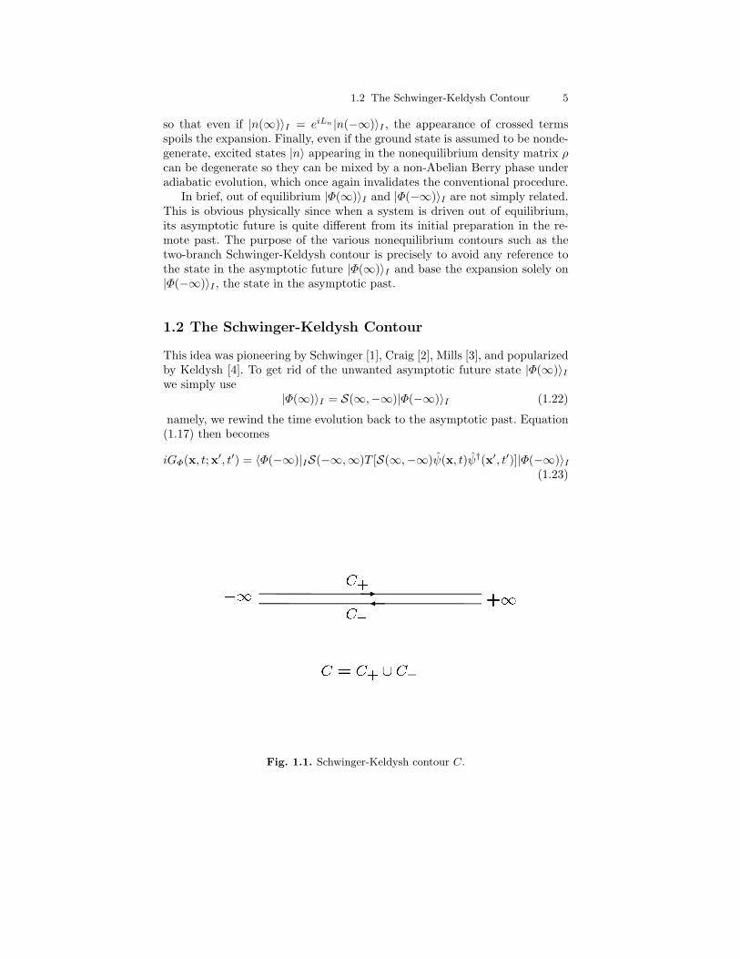
In brief, out of equilibrium |Φ(∞)〉I and |Φ(−∞)〉I are not simply related.This is obvious physically since when a system is driven out of equilibrium,its asymptotic future is quite different from its initial preparation in the re-mote past. The purpose of the various nonequilibrium contours such as thetwo-branch Schwinger-Keldysh contour is precisely to avoid any reference tothe state in the asymptotic future |Φ(∞)〉I and base the expansion solely on|Φ(−∞)〉I , the state in the asymptotic past.

1.2 The Schwinger-Keldysh Contour

This idea was pioneering by Schwinger [1], Craig [2], Mills [3], and popularizedby Keldysh [4]. To get rid of the unwanted asymptotic future state |Φ(∞)〉Iwe simply use

|Φ(∞)〉I = S(∞,−∞)|Φ(−∞)〉I (1.22)

namely, we rewind the time evolution back to the asymptotic past. Equation(1.17) then becomes

iGΦ(x, t;x′, t′) = 〈Φ(−∞)|IS(−∞,∞)T [S(∞,−∞)ψ(x, t)ψ†(x′, t′)]|Φ(−∞)〉I(1.23)

Fig. 1.1. Schwinger-Keldysh contour C.


Now we cannot simply push S(−∞,∞) past the time-ordering operator Tand merge it with the forward evolution S(∞,−∞), since the whole backwardevolution S(−∞,∞) lies to the left of the T -product. Left means later as faras time ordering is concerned. A clever way to kill these two birds with onestone is to introduce a two-branch contour C and ordering along this contourenforced by a contour-ordering operator Tc. This Schwinger-Keldysh contour(Fig. 1.1) consists of two oriented branches C = C+∪C−, the forward branchC+ extending from −∞ to ∞ and the backward branch C− extending from∞ to −∞. We now extend the time variables t, t′ to variables defined on thiscontour τ, τ ′, and define the fundamental object of nonequilibrium many-bodytheory, the contour-ordered Green’s function,

iG(x, τ ;x′, τ ′) = 〈Tc[ψ(x, τ)ψ†(x′, τ ′)]〉 = Tr ρTc[ψ(x, τ)ψ†(x′, τ ′)] (1.24)

With variables and ordering along the contour C, the interaction picture ex-pression corresponding to Eq. (1.23) is

iGΦ(x, τ ;x′, τ ′) = 〈Φ(−∞)|ITc[Sc(−∞,−∞)ψ(x, τ)ψ†(x′, τ ′)]|Φ(−∞)〉I(1.25)

where the contour S-matrix is

Sc(−∞,−∞) ≡ Tc exp(−i∮

C

dτ1 H′(τ1)

)(1.26)

where the integral is a line integral along the contour C. Note that there isno phase factor in the denominator as in the equilibrium theories since thecontour S-matrix by itself (i.e. not in a Tc-ordered product) is actually unity.

According to our previous discussion, the full Green’s function is now givenby

iG(x, τ ;x′, τ ′) = Tr ρ(−∞)Tc[Sc(−∞,−∞)ψ(x, τ)ψ†(x′, τ ′)] (1.27)

where we have a density matrix defined by

ρ(−∞) =∑Φ

pΦ|Φ(−∞)〉I〈Φ(−∞)|I (1.28)

where now the states are not the Heisenberg states |Φ〉 but the interactionpicture states in the remote past |Φ(−∞)〉I . From Eqs. (1.7) and (1.15), it isnot hard to show that

ρ = S(0,−∞)ρ(−∞)S(−∞, 0) (1.29)

So far this is rather general. Now, in the Keldysh theory we do adiabaticallyswitch on the nonequilibrium perturbation V according to eεt from the remotepast t = −∞ to the present t = 0, but we do not switch it off. This enables usto study stationary nonequilibrium states, a long time after the system has

1.3 The Closed Time Path Contour 7

been driven out of equilibrium2. Because of the adiabatic switch-on procedure,ρ(−∞) can be identified as the density matrix of the system in the remote pastwhen the nonequilibrium perturbation is turned off. It is then evolved in theusual way by the S-matrix S(0,−∞) to a nonequilibrium density matrix ρ.One thus usually chooses ρ(−∞) to be an equilibrium distribution, ρ(−∞) =e−βH/Z.

1.3 The Closed Time Path Contour

In the previous section, we constructed the perturbation expansion such thatthe Green’s function would be expressed as an average over the density matrixof the system in the remote past because this is what we know: because of theadiabatic switch-on procedure, we have ρ(−∞) = e−βH/Z which is explicitlyknown. Indeed, the idea of the Keldysh technique is that we want to avoidreference to the general nonequilibrium density matrix ρ which is not usuallyexplicitly known. However, this is not mandatory. If we actually know thedensity matrix ρ of the system at t = 0, then the early Eq. (1.13) is alreadyenough:

iG(x, τ ;x′, τ ′) = Tr ρTc[Sc(0, 0)ψ(x, τ)ψ†(x′, τ ′)] (1.30)

where ρ is now the full density matrix Eq. (1.7) at t = 0, and the contour overwhich the Tc operator and the S-matrix Sc are defined is the so-called closed

Fig. 1.2. Closed time path contour C0.

2 Actually, we may still study transient behavior in the Keldysh formalism, butprovided we use an explicitly time-dependent Hamiltonian and there are no initialcorrelations, namely, the initial density matrix has to be noninteracting.


time path contour C0 going from 0 to the latest of t or t′, and then back to0. Furthermore, there is nothing special about the time t = 0: we might havedefined the Heisenberg and interaction pictures with respect to some otherinitial time t0. Then the average would be over the density matrix at time t0:

iG(x, τ ;x′, τ ′) = Tr ρ(t0)Tc[Sc(t0, t0)ψ(x, τ)ψ†(x′, τ ′)] (1.31)

and the closed time path contour [5, 6] now goes from t0 to the latest oft or t′, and then back to t0 (Fig. 1.2). To recover the Schwinger-Keldyshcontour, we take the limit t0 → −∞ and insert a factor of S(t,∞)S(∞, t)or S(t′,∞)S(∞, t′) in the perturbation expansion Eq. (1.13) to extend thecontour to ∞, depending on whether t or t′ is the latest. The density matrixis now ρ(−∞) and we invoke the adiabatic switch-on procedure to chooseρ(−∞) = e−βH/Z.

1.4 Interactions: the Kadanoff-Baym Contour

Equation (1.31) is in a form suitable for a perturbation expansion providedthat ρ(t0) is a noninteracting (i.e., 1-particle) density matrix and that thefield operators ψ, ψ† in the interaction picture evolve with a noninteractingHamiltonian H. Indeed, these are the conditions of applicability of Wick’s the-orem [7]. They are satisfied in the Keldysh theory if H is noninteracting sincethen ρ(−∞) = e−βH/Z is a 1-particle density matrix. What if H containsinteractions?

Let us first keep a general t0 and assume that ρ(t0) = e−βH/Z with H ageneral interacting Hamiltonian. We can always take t0 → −∞ at the end torecover the Keldysh theory. We first break further the equilibrium HamiltonianH = H0 + V into a noninteracting part H0 and the interactions V . We wantto express the interacting density matrix e−βH in terms of a noninteractingone e−βH0 . We make use of Eqs. (1.11) and (1.12), but in imaginary timeand with a general initial time t0. Now the full (equilibrium) Hamiltonianis H. As mentioned earlier, we will therefore use upright letters U and Sfor the evolution and S-matrix respectively. The interaction and Heisenbergpictures are now defined with respect to the initial time t0, meaning thatA(t) = eiH(t−t0)Ae−iH(t−t0) and A(t) = eiH0(t−t0)Ae−iH0(t−t0). Since H istime-independent, the evolution operator is simply U(t, t0) = e−iH(t−t0) andwe have

S(t, t0) = eiH0(t−t0)U(t, t0) (1.32)

where the S-matrix is S(t, t′) = T exp(−i∫ t

t′dt1 V (t1)

). We then have

e−βH = e−βH0S(t0 − iβ, t0) (1.33)

where here the S-matrix S(t0 − iβ, t0) evolves the density matrix along acontour [t0, t0 − iβ] on the imaginary axis. The Green’s function Eq. (1.31)now assumes the form

1.4 Interactions: the Kadanoff-Baym Contour 9

iG(1, 1′) =1Z

Tr e−βH0S(t0 − iβ, t0)Tc[Sc(t0, t0)ψH(1)ψ†H(1′)] (1.34)

where for simplicity we denote space and time arguments by a collective in-dex 1 ≡ (x, τ), 1′ ≡ (x′, τ ′). We have also explicitly indicated that the fieldoperators still evolve according to the full H, see Eq. (1.9). They have to bebrought to the current interaction picture defined with respect to H0. Thiscan be achieved as previously through the S-matrix,

ψH(x, t) = S(t0, t)ψ(x, t)S(t, t0) (1.35)

where the caret without the subscript denotes the interaction picture withrespect to H0. Equation (1.34) thus becomes

iG(1, 1′) =1Z

Tr e−βH0S(t0 − iβ, t0)

×Tc[Sc(t0, t0)S(t0, t)ψ(1)S(t, t0)S(t0, t′)ψ†(1′)S(t′, t0)] (1.36)

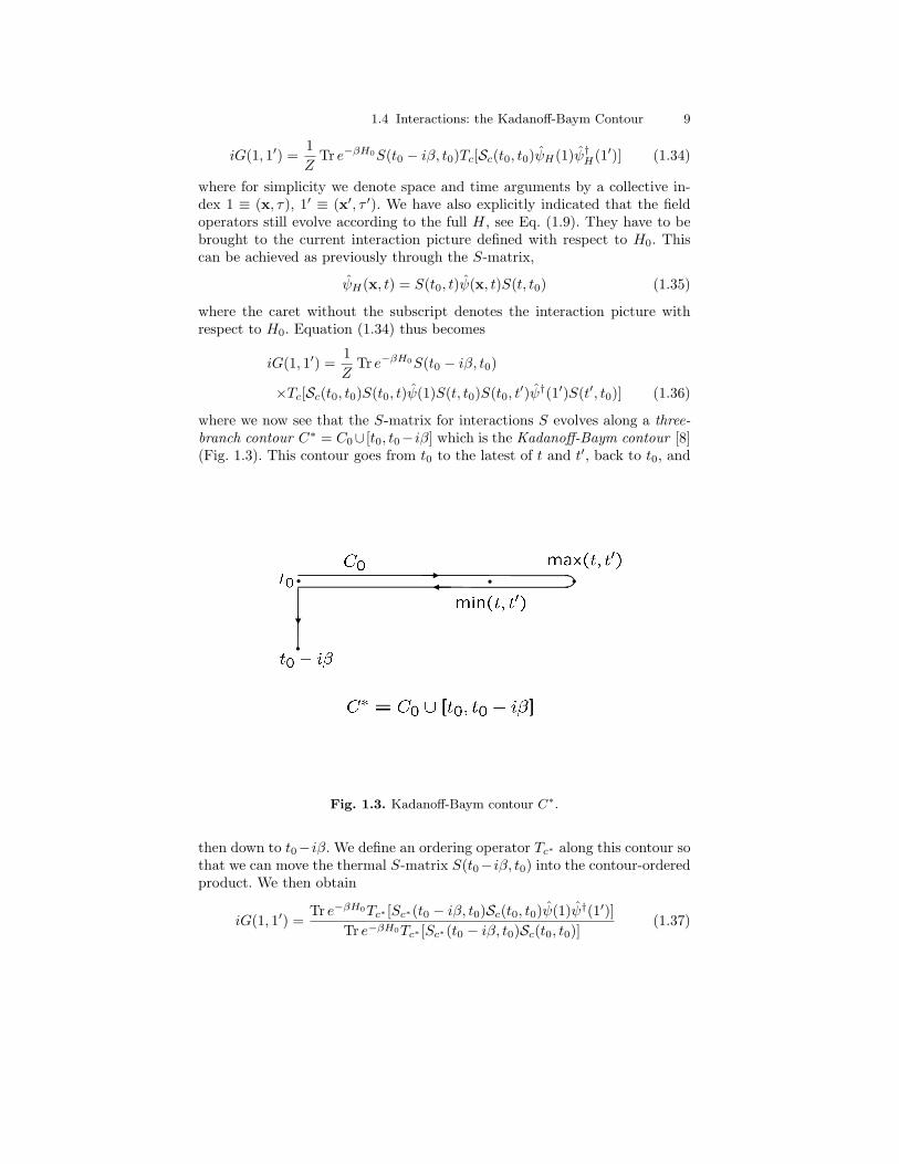
where we now see that the S-matrix for interactions S evolves along a three-branch contour C∗ = C0∪ [t0, t0−iβ] which is the Kadanoff-Baym contour [8](Fig. 1.3). This contour goes from t0 to the latest of t and t′, back to t0, and

Fig. 1.3. Kadanoff-Baym contour C∗.

then down to t0−iβ. We define an ordering operator Tc∗ along this contour sothat we can move the thermal S-matrix S(t0−iβ, t0) into the contour-orderedproduct. We then obtain

iG(1, 1′) =Tr e−βH0Tc∗ [Sc∗(t0 − iβ, t0)Sc(t0, t0)ψ(1)ψ†(1′)]

Tr e−βH0Tc∗ [Sc∗(t0 − iβ, t0)Sc(t0, t0)](1.37)


where in analogy with Eq. (1.26) we define a new contour-ordered S-matrixdefined along the Kadanoff-Baym contour,

Sc∗(t0 − iβ, t0) ≡ Tc∗ exp(−i∫

C∗dτ1 V (τ1)

)(1.38)

We have written the partition function as

Z = Tr e−βH = Tr e−βH0S(t0− iβ, t0) = Tr e−βH0Tc∗ [Sc∗(t0− iβ, t0)Sc(t0, t0)](1.39)

since the S-matrices are already time-ordered on their respective contours,and since times on the [t0, t0− iβ] strip are always later than times on C0, wesimply have Sc(t0, t0) = 1 and Sc∗(t0 − iβ, t0) = S(t0 − iβ, t0) even inside theTc∗ -ordered product. Note that the time arguments in Eq. (1.37) are definedon the three-branch Kadanoff-Baym contour C∗. Equation (1.37) is now fitfor perturbation theory since by assumption the averages are with respect toa 1-particle density matrix e−βH0 and the field operators evolve according tothe noninteracting H0, so Wick’s theorem can be applied.

The Kadanoff-Baym formalism is adequate for the study of initial corre-lations, namely the effect for times t > t0 of having an interacting densitymatrix at time t0, without the assumption t t0. The price to pay for thispowerful formalism is that the Green’s function is defined on a three-branchcontour and has a complicated expression in terms of the simultaneous per-turbation expansion of two S-matrices. However for many practical purposesthis is overkill, and for steady-state problems we do not care about the effectof initial correlations. In many cases we can assume that correlations decay intime so that if we take the limit t0 → −∞, at any finite time t t0 there isno signature left of the correlations in the initial density matrix ρ(t0). This isthe Bogoliubov principle of weakening correlations, a general principle in non-equilibrium statistical mechanics. It is however advised to keep in mind thatin some cases initial correlations can persist at long times due for example tothe presence of metastable states.

1.4.1 Neglect of Initial Correlations and Schwinger-Keldysh Limit

For most practical purposes we can safely ignore the initial correlations whentaking the limit t0 → −∞. It has been shown [9, 10, 11] that neglectinginitial correlations amounts to neglecting the imaginary strip [t0, t0−iβ] in theKadanoff-Baym contour, so we are back with the Schwinger-Keldysh contour(after having extended the closed time path contour as explained in section1.3). In this limit, the S-matrices in the denominator of Eq. (1.37) are trivialand the denominator is just Tr e−βH0 . We thus have

iG(1, 1′) = Tr ρ0Tc[Sc(−∞,−∞)Sc(−∞,−∞)ψ(1)ψ†(1′)] (1.40)

where the noninteracting density matrix is just

1.5 Contour Dyson Equation 11

ρ0 ≡e−βH0

Tr e−βH0(1.41)

and Sc(−∞,−∞) is just the Kadanoff-Baym contour-ordered S-matrix ofEq. (1.38) but neglecting the third branch of the contour and taking the limitt0 → −∞,

Sc(−∞,−∞) ≡ Tc exp(−i∮

C

dτ1 V (τ1))

(1.42)

so that now all the ordering takes place along the Schwinger-Keldysh contourC. If the system is initially at zero temperature, we simply have

iG(1, 1′) = 〈Φ0|Tc[Sc(−∞,−∞)Sc(−∞,−∞)ψ(1)ψ†(1′)]|Φ0〉 (1.43)

with |Φ0〉 the noninteracting ground state of H0. We see that we have nowalmost recovered Eq. (1.27), albeit with an additional S-matrix Sc contain-ing the effect of the interactions V . We summarize both zero and finite-temperature results Eqs. (1.43) and (1.40) in the formula

iG(1, 1′) = 〈Tc[Sc(−∞,−∞)Sc(−∞,−∞)ψ(1)ψ†(1′)]〉 (1.44)

with the suitable expectation value. This is the essential starting point for cal-culations in Keldysh theory. The perturbation expansion can now be carriedout, with both nonequilibrium terms H ′ from Sc (Eq. (1.26)) and interactionterms V from Sc (Eq. (1.38)) appearing in the expansion and in the ensuingFeynman diagrams. Let us remark here that the power of the Kadanoff-Baymand Keldysh approaches to nonequilibrium many-body theory – or more gen-erally, to nonequilibrium field theory – lies in its structure being formallyidentical to that of usual equilibrium many-body theory, albeit with a timeevolution and the corresponding perturbative expansion defined on a moregeneral contour. Then most of the tools of quantum field theory can be ap-plied: Feynman diagrams, integral equations for vertex functions such as theDyson equation, etc.

1.5 Contour Dyson Equation

The whole perturbation expansion for the contour-ordered 1-particle Green’sfunction on the nonequilibrium contour C can be resummed in the form of anintegral equation, the Dyson equation:

G(1, 1′) = G0(1, 1′) +∫d2G0(1, 2)U(2)G(2, 1′)

+∫d2∫d3G0(1, 2)Σ(2, 3)G(3, 1′) (1.45)

G(1, 1′) = G0(1, 1′) +∫d2G(1, 2)U(2)G0(2, 1′)

+∫d2∫d3G(1, 2)Σ(2, 3)G0(3, 1′) (1.46)


where G(1, 1′) ≡ −i〈Tc[ψ(1)ψ†(1′)]〉 is the exact Green’s function Eq. (1.24)and G0(1, 1′) ≡ −i〈Tc[ψ(1)ψ†(1′)]〉 is the unperturbed Green’s function withfield operators in the interaction picture, U(2) is a 1-particle potential andΣ(2, 3) is the 1-particle irreducible self-energy. The integral sign means a sumover all internal variables,

∫d2 ≡

∑σ2

∫dx2

∫Cdτ2. For simplicity, we will use

the following notation,

G = G0 +G0UG+G0ΣG (1.47)G = G0 +GUG0 +GΣG0 (1.48)

1.6 Initial Correlations with Arbitrary Initial DensityMatrix

For the sake of completeness, let us just mention a few words about themost general problem (as far as I know) although we won’t actually try tosolve it in these lectures. Consider Eq. (1.31). In the Keldysh theory we lett0 → −∞ and neglected initial correlations. In the Kadanoff-Baym theory weconsidered initial correlations by keeping a finite t0, but we assumed that theinitial density matrix ρ(t0) had the equilibrium form ρ(t0) = e−βH/Z with Han interacting Hamiltonian. Now, what if ρ(t0) is a general, nonequilibrium,interacting density matrix? This corresponds to preparing the system in acorrelated nonequilibrium state at a given time t0 and observing the timeevolution of the system for finite times t > t0 without assuming t t0. Peopleneed that in the study of correlated plasmas for example. This problem hasbeen studied by Fujita [9], Hall [10], Kukharenko and Tikhodeev [11], andWagner [12] who gives a rather clear and comprehensive discussion. The ideais to use a modified Kadanoff-Baym contour. First, the general nonequilibriumdensity matrix can still be written in the form

ρ(t0) =e−λB

Tr e−λB(1.49)

since it is positive definite and Hermitian, where λ is not the temperatureand B is not the Hamiltonian but some general quantities. But because of theformal analogy to β and H, we can setup a perturbation expansion on a mod-ified Kadanoff-Baym contour with the imaginary strip [t0 − iλ, t0]. This verygeneral approach encompasses the Feynman, Matsubara, Schwinger-Keldysh,and Kadanoff-Baym approaches as special cases [12].

1.7 Relation to Real-Time Green’s Functions

In all that follows, we will confine ourselves exclusively to the Keldysh ap-proach [4, 14, 16, 13, 15] (but the equilibrium Hamiltonian H can still contain

1.7 Relation to Real-Time Green’s Functions 13

interactions). Let us recap. Our initial goal is to calculate the real-time Green’sfunction of Eq. (1.1),

iG(x, t;x′, t′) = 〈T [ψ(x, t)ψ†(x′, t′)]〉 = Tr ρT [ψ(x, t)ψ†(x′, t′)] (1.50)

with operators in the Heisenberg picture with respect to the full nonequilib-rium Hamiltonian H and a nonequilibrium density matrix ρ. We have defineda contour-ordered Green’s function Eq. (1.24) with time arguments on a con-tour C,

iG(x, τ ;x′, τ ′) = 〈Tc[ψ(x, τ)ψ†(x′, τ ′)]〉 (1.51)

and obtained a perturbation expansion for that Green’s function in Eq. (1.44),

iG(x, τ ;x′, τ ′) = 〈Tc[Sc(−∞,−∞)Sc(−∞,−∞)ψ(x, τ)ψ†(x′, τ ′)]〉 (1.52)

with operators in the interaction picture with respect to the noninteract-ing part H0 of the equilibrium Hamiltonian H. Now, how is the contour-ordered Green’s function Eq. (1.51) related to the real-time Green’s functionEq. (1.50)?

The answer is that depending on which branch the contour arguments τ, τ ′

belong to, different real-time Green’s functions are obtained:

G(x, τ ;x′, τ ′) =

GT (x, t;x′, t′) ≡ −i〈T [ψ(x, t)ψ†(x′, t′)]〉 if τ, τ ′ ∈ C+,G<(x, t;x′, t′) ≡ i〈ψ†(x′, t′)ψ(x, t)〉 if τ ∈ C+, τ

′ ∈ C−,G>(x, t;x′, t′) ≡ −i〈ψ(x, t)ψ†(x′, t′)〉 if τ ∈ C−, τ ′ ∈ C+,

GT (x, t;x′, t′) ≡ −i〈T [ψ(x, t)ψ†(x′, t′)]〉 if τ, τ ′ ∈ C−,(1.53)

where GT is the time-ordered Green’s function of Eq. (1.50) and T is an anti-time ordering operator which orders operators in the opposite way as T , sothat GT is the anti-time-ordered Green’s function. G<,> are the lesser andgreater Green’s functions, respectively. One then defines a 2×2 matrix Green’sfunction in real time,

G =(GT G<

G> GT

)=(G11 G12

G21 G22

)(1.54)

It is not hard to show from the definitions that the following identities hold,

GR = GT −G< = G> −GT (1.55)

GA = GT −G> = G< −GT (1.56)

GK = G> +G< = GT +GT (1.57)

1.7.1 Larkin-Ovchinnikov Representation

In the so-called Larkin-Ovchinnikov representation [16], we perform a lineartransformation on G to obtain another matrix G,


G = Lτ3GL† =(GR GK

0 GA

)(1.58)

where L = 1√2(τ0 − iτ2) where τ i are the Pauli matrices (τ0 is unity). GR,A

are the retarded and advanced Green’s functions,

GR(x, t;x′, t′) = −iθ(t− t′)〈ψ(x, t), ψ†(x′, t′)〉 (1.59)GA(x, t;x′, t′) = iθ(t′ − t)〈ψ(x, t), ψ†(x′, t′)〉 (1.60)

and GK is the Keldysh Green’s function,

GK(x, t;x′, t′) = −i〈[ψ(x, t), ψ†(x′, t′)]〉 (1.61)

1.7.2 Langreth Theorem of Analytic Continuation

Consider the ‘matrix products’ occurring in Eqs. (1.45) and (1.46). These areconvolution integrals on the two-branch contour. Consider first the followingproduct of two contour-ordered quantities (such as Green’s functions or self-energies),

C(1, 1′) =∫d2A(1, 2)B(2, 1′) (1.62)

or in simple matrix notation,C = AB (1.63)

How do we convert this product to an integral over the real axis involvingthe real-time components of A and B? This is accomplished by the Langreththeorem [18, 19] which consists in a series of rules:

(AB)<> = ARB

<> +A

<>BA (1.64)

(AB)R,A = AR,ABR,A (1.65)

(ABC)<> = ARBRC

<> +ARB

<>CA +A

<>BACA (1.66)

(ABC)R,A = AR,ABR,ACR,A (1.67)

where the ‘matrix products’ on the right-hand side consist in summationsover internal degrees of freedom (space and spin) and convolution integralson the real axis from −∞ to ∞. We are now completely rid of the contour;the 2 × 2 matrix structure takes care of the nonequilibrium physics and wecan use ordinary real-time integrals. In particular, we can Fourier transformto frequency space in the case of a nonequilibrium steady state in which theGreen’s functions are time-translationally invariant, Gij(t, t′) = Gij(t− t′).

We will not derive all these rules but only show how the first one can beobtained. Consider C = AB on the Schwinger-Keldysh contour C. Then

1.7 Relation to Real-Time Green’s Functions 15

C<(t, t′) =∫

C

dτ1A(t, τ1)B(τ1, t′)

=∫ ∞

−∞dt1A

T (t, t1)B<(t1, t′) +∫ −∞

∞dt1A

<(t, t1)BT (t1, t′)

=∫ ∞

−∞dt1

[AT (t, t1)B<(t1, t′)−A<(t, t1)BT (t1, t′)

]From Eqs. (1.55) and (1.56), we know that AT = AR+A< and BT = B<−BA,hence

C<(t, t′) =∫ ∞

−∞dt1[(AR(t, t1) +A<(t, t1)

)B<(t1, t′)−A<(t, t1)

(B<(t1, t′)−BA(t1, t′)

)]=∫ ∞

−∞dt1[AR(t, t1)B<(t1, t′) +A<(t, t1)BA(t1, t′)

]The other rules are obtained in a similar fashion. Usually, one writes downthe diagrams as in conventional many-body theory and the correspondinganalytic expressions involving contour-ordered Green’s functions. Typically,these involve integrals over the contour. Then one translates these expressionsin the real-time language using the Langreth rules. This is often referred toas ‘analytic continuation’ from the contour to the real-time axis in analogywith the Matsubara formalism. We feel this is somewhat pedantic since theSchwinger-Keldysh contour is not really a contour in the complex plane; it isonly two counter-propagating copies of the real axis.

2

Quantum Kinetic Equations

We have now set up the necessary machinery to construct quantum kineticequations which govern the evolution of correlation functions in a quantummany-body system driven out of equilibrium. We first say ‘correlation func-tions’ which are two-time objects instead of ‘distribution functions’ whichare one-time objects because equations typically do not close for distributionfunctions. However equations for correlation functions are very complicatedintegral equations which can usually only be solved numerically. There how-ever exists a variety of useful approximations which make the equations fordistribution functions close.

We will thus first discuss the Keldysh and Kadanoff-Baym equations whichare exact quantum kinetic equations for the nonequilibrium correlation func-tions of the system. Then we will introduce the Wigner transform, the gradientexpansion and the gradient approximation which yield the quantum Boltz-mann equation (QBE). As this equation is still rather complicated, furtherapproximations can be made such as the quasiparticle and quasiclassical ap-proximations. The QBE is still an equation for a four-parameter (two-point)correlation function G<(p, ω,R, T ). Expressed in terms of the Wigner dis-tribution function fW (p,R, T ) ≡ −iG<(p, t = 0,R, T ) which is a one-timefunction, the QBE does not close. One can however generate a closed equationfor the Wigner distribution function by introducing the so-called generalizedKadanoff-Baym ansatz [17]. We will also recover the classical Boltzmann equa-tion as a limiting case of the QBE.

We can actually understand from simple arguments why a kinetic equationfor a quantum distribution function should have more terms than that for aclassical distribution function. Recall how the classical Boltzmann equationis derived. Because of the incompressibility of phase space, the total rate ofchange of the classical distribution function f(p,R, T ) is equal to the rate ofchange of f due to collisions, say

(∂f∂T

)coll

≡ I[f ]:

df

dT= I[f ]

18 2 Quantum Kinetic Equations

The Boltzmann equation is then obtained simply by using the chain rule forderivatives, (

∂

∂T+ v · ∇R + F · ∇p

)f = I[f ] (2.1)

since dR/dT = v is the velocity and dp/dT = F is the force from Newton’ssecond law. In the quantum mechanical case, the distribution function alsohas an energy argument ω: f = f(p, ω,R, T ). We thus generate an additionalterm in the corresponding Boltzmann equation:(

∂

∂T+ v · ∇R + F · ∇p +

dω

dT

∂

∂ω

)f = I[f ]

But the rate of change of energy is just the power, dω/dT = P = F · v.Considering electric and magnetic fields, the force is just the Lorentz forceF = e(E + v×B), so dω/dT = eE · v since the magnetic force does no work.Hence we obtain [13][

∂

∂T+ v ·

(∇R + eE

∂

∂ω

)+ e(E + v ×B) · ∇p

]f = I[f ] (2.2)

We will see later in this chapter that this is essentially the structure of theQBE.

2.1 Keldysh Equation

We first apply the fourth Langreth rule Eq. (1.67) to the contour Dysonequations (1.47) and (1.48). We obtain

GR,A = GR,A0 +GR,A

0 UGR,A +GR,A0 ΣR,AGR,A (2.3)

GR,A = GR,A0 +GR,AUGR,A

0 +GR,AΣR,AGR,A0 (2.4)

because a one-body potential U is proportional to a delta function in time (in-stantaneous) and is thus neither retarded nor advanced. Hence we see that theretarded and advanced nonequilibrium Green’s functions obey Dyson equa-tions which are formally identical to the equilibrium Dyson equations. If wenow apply the third Langreth rule Eq. (1.66), we obtain

G<> = G

<>0 +GR

0 UG<> +G

<>0 UG

A +GR0 Σ

RG<> +GR

0 Σ<>GA +G

<>0 Σ

AGA

G<> = G

<>0 +GRUG

<>0 +G

<>UGA

0 +GRΣRG<>0 +GRΣ

<>GA

0 +G<>ΣAGA

0

because the instantaneous one-body potential is diagonal in Keldysh space

(U<> = 0). These two equations are the Keldysh equations. Integration over

the real axis is understood, for example

2.1 Keldysh Equation 19

(GR0 UG

<)(x, t;x′, t′) =∫ ∞

−∞dt1

∫dx1G

R0 (x, t;x1, t1)U(x1, t1)G<(x1, t1;x′, t′)

and

(GR0 Σ

RG<)(x, t;x′, t′) =∫ ∞

−∞dt1

∫dx1

∫ ∞

−∞dt2

∫dx2G

R0 (x, t;x1, t1)

×ΣR(x1, t1;x2, t2)G<(x2, t2;x′, t′)

The Keldysh equations can be iterated. The infinite order iterate of eitherequation gives the same following explicit equation for G<,

G<> = [1 +GR(U +ΣR)]G

<>0 [1 + (U +ΣA)GA] +GRΣ

<>GA (2.5)

which is the usual general form of the Keldysh equation.We now digress a moment to study the free Green’s functions G<,>,R,A

0

more closely. They are propagators for a noninteracting HamiltonianH0. To befully general, we consider a multiband one-particle Hamiltonian Hµν

0 (x,−i∇)where µ, ν are band (and/or spin) indices. We however require that each Hµν

0

be a properly symmetrized function of the conjugate variables,

Hµν0 (x,−i∇) =

∑i

fµνi (x), gµν

i (−i∇)+ uµν(x) + vµν(−i∇) (2.6)

Then Hermiticity of the second quantized Hamiltonian,

H0 =∑µν

∫dxψ†µ(x)Hµν

0 (x,−i∇)ψν(x), (2.7)

requires that1

Hµν0 (x,−i∇) = Hνµ

0 (x, i∇)∗ (2.8)

We use a matrix notation where Gµν0 is represented by a matrix G0 in band

space. It is easy to show by application of the equation of motion tech-nique that the contour-ordered propagator G0(x, τ ;x′, τ ′) satisfies the fol-lowing equations of motion2 where matrix multiplication in band space isunderstood,

1 Two remarks. First, in the case that the only imaginary quantities in Hµν0 come

from −i∇ (for example for a spin system without Zeeman term and in the absenceof spin-orbit coupling), Eq. (2.8) requires the matrix Hµν

0 to be symmetric. Sec-ond, if Hµν

0 depends only on x and not on −i∇ (for example for a tight-bindingmodel where x becomes a discrete variable and∇ is replaced by finite differences),Eq. (2.8) requires the matrix Hµν

0 to be Hermitian.2 The delta function δ(τ, τ ′) is defined on the contour, such that δR,A(t, t′) = δ(t−t′)

and δ<>(t, t′) = 0.

20 2 Quantum Kinetic Equations(i∂τ −H0(x,−i∇)

)G0(x, τ ;x′, τ ′) = δ(x− x′)δ(τ, τ ′) (2.9)

G0(x, τ ;x′, τ ′)(−i∂τ ′ −H0(x′, i∇′)

)= δ(x− x′)δ(τ, τ ′) (2.10)

where in Eq. (2.10) the derivatives ∂τ ′ and ∇′ act to the left. We do not writeexplicitly unit matrices in band space. If we take the real-time components ofthese contour equations, we obtain(

i∂t −H0(x,−i∇))GR,A

0 (x, t;x′, t′) = δ(x− x′)δ(t− t′) (2.11)(i∂t −H0(x,−i∇)

)G<,>

0 (x, t;x′, t′) = 0 (2.12)

GR,A0 (x, t;x′, t′)

(−i∂t′ −H0(x′, i∇′)

)= δ(x− x′)δ(t− t′) (2.13)

G<,>0 (x, t;x′, t′)

(−i∂t′ −H0(x′, i∇′)

)= 0 (2.14)

We can write in simplified notation

G−10 GR,A

0 = 1 (2.15)

G−10 G

<>0 = 0 (2.16)

GR,A0 G−1

0 = 1 (2.17)

G<>0 G

−10 = 0 (2.18)

where the action of the operator G−10 on the right and on the left is defined

in Eqs. (2.11)-(2.14). These relations will be helpful in deriving the Kadanoff-Baym and quantum Boltzmann equations in the next section.

The Keldysh equations are used directly in mesoscopic transport for ex-ample, where one studies finite-sized nonequilibrium systems with importantspatial and/or temporal inhomogeneities. Then the continuous spatial argu-ments x,x′ in the Green’s functions are typically replaced by discrete siteindices i, j (i.e. in a tight-binding representation) or by principal quantumnumbers n, n′ for discrete energy levels (i.e. in quantum dot physics). TheGreen’s functions then become finite-sized matrices and the Keldysh equa-tions become matrix equations. For a finite-sized system, it is possible toshow that the Keldysh equation (2.5) becomes

G<> = GRG−1

0 G<>0 [1 + (U +ΣA)GA] +GRΣ

<>GA (2.19)

but the first term vanishes by Eq. (2.16), so that we have

G<> = GRΣ

<>GA (2.20)

which is the form of the Keldysh equation that is used in mesoscopic transport.

2.2 Kadanoff-Baym Equation 21

At the other side of the spectrum, if one wishes to study transport inmacroscopic samples, i.e. transport in metals or bulk semiconductors, non-equilibrium (but not mesoscopic) superconductivity, etc., then it is usuallymore practical to use the Kadanoff-Baym equation and its ensuing Boltzmann-type approximations to be studied in the next sections [16]. Then one has tosolve an (integro-)differential equation. It is easier to make approximations(such as near-homogeneous or slowly-varying perturbations, not too far fromequilibrium) on the Kadanoff-Baym equation than on the Keldysh equation.Furthermore, a connection to conventional transport formalisms such as linearresponse theory (Kubo formula) can be made: transport coefficients calculatedfrom the linearized quantum Boltzmann equation (which can be derived fromthe Kadanoff-Baym equation) in the steady-state limit are identical to thoseobtained in linear response theory.

2.2 Kadanoff-Baym Equation

With the help of these relations, we are now able to derive the Kadanoff-Baymequation from the Keldysh equations. If we act with G−1

0 on the left of thefirst Keldysh equation and on the right of the second Keldysh equation anduse relations (2.15)-(2.18), we obtain

(G−10 − U)G< = ΣRG< +Σ<GA (2.21)

G<(G−10 − U) = GRΣ< +G<ΣA (2.22)

We now subtract these equations from one another:

[G−10 − U,G<] = ΣRG< +Σ<GA −GRΣ< −G<ΣA (2.23)

We now introduce the nonequilibrium spectral function A ≡ i(GR − GA)and the scattering rate, or linewidth, or imaginary part of the self-energyΓ ≡ i(ΣR − ΣA). We also define symmetric combinations or real parts asReG ≡ 1

2 (GR +GA) and ReΣ ≡ 12 (ΣR +ΣA). In terms of these quantities,

Eq. (2.23) can be written as

[G−10 − U,G<]− [ReΣ,G<]− [Σ<,ReG] = − i

2

(Γ,G< − A,Σ<

)However, as seen before, the Keldysh components GR,A,<,> and ΣR,A,<,>

are not independent. With the relations −iA = GR − GA = G> − G< and−iΓ = ΣR −ΣA = Σ> −Σ< we can rewrite the equation as

[G−10 − U − ReΣ,G<]− [Σ<,ReG] = 1

2

(Σ>, G< − G>, Σ<

)(2.24)

which is the Kadanoff-Baym equation [8, 13]. As we will see, the term onthe left-hand side involving [G−1

0 − U,G<] is a driving term, while the termsinvolving ReΣ and ReG describe renormalization effects. From a transport


point of view, they lead to renormalized transport coefficients and are ne-glected in the classical Boltzmann limit. The right-hand side is a collisionterm as will be seen. A similar Kadanoff-Baym equation can be derived forG>. By subtracting the two equations, one obtains an equation for the spectralfunction,

[G−10 − U − ReΣ,A]− [Γ,ReG] = 0 (2.25)

which is used as a consistency check when one looks for approximate solutionsto the Kadanoff-Baym equation.

The Kadanoff-Baym equation has to be supplemented by an equation forthe retarded and advanced Green’s functions. It is obtained in the same way,applying relations (2.15)-(2.18) to the nonequilibrium Dyson equations (2.3)-(2.4):

(G−10 − U)GR = 1 +ΣRGR (2.26)

GR(G−10 − U) = 1 +GRΣR (2.27)

Add these two equations and dividing by 2 gives

12G

−10 − U,GR = 1 + 1

2ΣR, GR (2.28)

In practice, because self-energies are typically functionals of the Green’s func-tion Σ = Σ[G], the Kadanoff-Baym equation and the equations of motion(2.26)-(2.27) for GR have to be solved self-consistently. Needless to say, this isa rather difficult task and one often has to resort to numerical techniques. Ap-proximations have to be made for the self-energy functions. However, theseapproximations cannot be made blindly by choosing an arbitrary subset ofdiagrams since it is then possible to violate conservation laws as shown byBaym and Kadanoff. Self-energies should be derived from the Luttinger-Ward[20] functional Φ,

Σ[G] =δΦ[G]δG

(2.29)

The Luttinger-Ward functional Φ[G] is defined diagrammatically as the sumof all skeleton connected vacuum diagrams with free propagators G0 replacedby exact propagators G. In practice, one keeps only a few diagrams in thediagrammatic expansion of Φ and then obtains the corresponding diagram-matic representation of the self-energy Σ[G] by removing a fermion line G(which corresponds to functional differentiation in Eq. (2.29)). These so-calledΦ-derivable approximations preserve conservation laws and are termed con-serving approximations [21, 22, 8]. For interacting systems involving coupleddegrees of freedom such as electrons and phonons, the electron self-energy Σand phonon polarization Π should be derived from the same electron-phononvertex Γ . This ensures that the same level of approximation is maintainedfor both the electron and phonon subsystems [23]. In general, gauge invari-ance implies the Ward identities which relate the self-energies and the vertexso that a given Φ-derivable approximation for the self-energy Σ[G] defines a


fully consistent level of approximation for Green’s functions, self-energies, andthe vertex.

2.2.1 Wigner Representation and Gradient Expansion

We now move on to the gradient expansion of the Kadanoff-Baym equation[8, 16, 24]. The idea is to separate slow macroscopic variations from fastmicroscopic variations, and then perform a gradient expansion on the slowvariables. In order to do that, we introduce mixed coordinates, the so-calledWigner representation:

r ≡ x1 − x2, R ≡ 12 (x1 + x2) (2.30)

t ≡ t1 − t2, T ≡ 12 (t1 + t2) (2.31)

so that a function C(x1, t1;x2, t2) becomes a function C(r, t,R, T ). The fast‘relative’ variables (r, t) will be Fourier transformed to (k, Ω) while the slow‘center-of-mass’ variables3 (R, T ) will serve for the gradient expansion. TheFourier transform is defined as

C(k, Ω,R, T ) ≡∫dt

∫dr ei(Ωt−k·r)C(r, t,R, T ) (2.32)

=∫dt

∫dr ei(Ωt−k·r)C

(R + 1

2r, T + 12 t;R− 1

2r, T −12 t)

We first work out the Wigner transform of the driving commutator term[G−1

0 − U,G<]. We have

[G−10 − U,G<]x1,x2 =

(i∂

∂t1−H0(x1,−i∇1)− U(x1)

)G<(x1, x2)

−G<(x1, x2)(−i ∂∂t2

−H0(x2, i∇2)− U(x2))

and for convenience we use a four-vector notation xµ1,2 = (t1,2,x1,2).

We want to study the dynamics of a system driven out of equilibriumby constant and uniform external electric E and magnetic B fields4. We firstconcentrate on the electric field and the magnetic field will be added later. The

3 For example, consider a free propagator g(t1, t2) = −ie−i$(t1−t2) where $ issome characteristic frequency. Considered as a function of t = 1

2(t1 − t2) and

T = 12(t1 + t2), this function has a fast variation with frequency 2$ in the t

variable and is constant (infinitely slow variation) in the T variable. If we add aslow disturbance $ → $ + ∆(t), there will start to be a weak dependence in T ,but slower than the dependence in t.

4 All the following derivations can be done for a general one-particle potential U(x)but would lead to extremely cumbersome expressions. This doesn’t have muchinterest anyway since the physically relevant perturbations are E and B fields.


one-particle potential U(x) contains the electric field in the scalar potentialgauge:

U(x) = −eE · x (2.33)

We have

[G−10 − U,G<]x1,x2 =

(i∂

∂t1+ i

∂

∂t2

)G<(x1, x2)−H0(x1,−i∇1)G<(x1, x2)

+G<(x1, x2)H0(x2, i∇2) + eE · (x1 − x2)G<(x1, x2)

The change of variables Eqs. (2.30) and (2.31) imply the following relationsfor the derivatives,

∂

∂T=

∂

∂t1+

∂

∂t2,

∂

∂t=

12

(∂

∂t1− ∂

∂t2

),

and similar relations for the spatial derivatives. In Wigner coordinates we thushave

[G−10 − U,G<]r,t,R,T = i

∂

∂TG<(r, t,R, T )−H0

(R + 1

2r,−i(12∇R +∇r)

)G<

+G<H0

(R− 1

2r, i(12∇R −∇r)

)+ eE · rG<

We now perform the Fourier transformation of the center-of-mass variablesEq. (2.32), which corresponds to the following substitutions,

i∂

∂t→ Ω (2.34)

−i∇r → k (2.35)

t → −i ∂∂Ω

(2.36)

r → i∇k (2.37)

We obtain

[G−10 − U,G<]k,Ω,R,T = i

∂

∂TG<(k, Ω,R, T )−H0

(R + i

2∇k,k− i2∇R

)G<

+G<H0

(R− i

2∇k,k + i2∇R

)+ ieE · ∇kG

<

We now perform a change of variables introduced by Mahan and Hansch,

ω = Ω + eE ·R (2.38)

which eliminates an unphysical ∝ E · R term in the equation for GR to bederived later. This change of variables implies the following substitutions,

Ω → ω − eE ·R (2.39)

∇R → ∇R + eE∂

∂ω(2.40)


The derivative ∂/∂ω is important and differentiates the QBE from the classicalBoltzmann equation. We thus obtain the following final exact form for thedriving commutator in the Wigner representation,

[G−10 − U,G<]k,ω,R,T = i

∂G<

∂T−H0

(R + i

2∇k,k− i2

(∇R + eE

∂

∂ω

))G<

+G<H0

(R− i

2∇k,k + i2

(∇R + eE

∂

∂ω

))+ ieE · ∇kG

<

(2.41)

where G< = G<(k, ω,R, T ). We now see the importance of a proper orderingof the Hamiltonian since [R,∇R] 6= 0 and [k,∇k] 6= 0. The driving anti-commutator G−1

0 − U,GR appearing in Eq. (2.28) for the retarded Green’sfunction can be derived in a similar way. We simply quote the result:

12G

−10 − U,GRk,ω,R,T = ωGR − 1

2H0

(R + i

2∇k,k− i2

(∇R + eE

∂

∂ω

))GR

− 12G

RH0

(R− i

2∇k,k + i2

(∇R + eE

∂

∂ω

))(2.42)

where as advertised the unphysical term E · R is removed by the Mahan-Hansch transformation Eq. (2.38).

Having derived the driving terms in the Wigner representation, we mustnow see how to transform products of the form AB,

(AB)x1,t1;x2,t2 =∫dt′∫dx′A(x1, t1;x′, t′)B(x′, t′;x2, t2) (2.43)

From the definition of the Wigner coordinates Eqs. (2.30-2.31), we have

A(x1, t1;x′, t′) = A(x1 − x′, t1 − t′, 12 (x1 + x′), 1

2 (t1 + t′))

= A(x1 − x′, t1 − t′,R +

x′ − x2

2, T +

t′ − t22

)(2.44)

and similarly

B(x′, t′;x2, t2) = B(x′ − x2, t′ − t2,

12 (x′ + x2), 1

2 (t′ + t2))

= B(x′ − x2, t

′ − t2,R +x′ − x1

2, T +

t′ − t12

)(2.45)

Since the derivative is the generator of translations, we have the followingcompact form for the usual Taylor expansion,

f(R + a, T + s) = ea·∇Res∂T f(R, T ) (2.46)

Using Eqs. (2.44,2.45,2.46), we can write Eq. (2.43) as


(AB)x1,t1;x2,t2 =∫dt′∫dx′A(x1 − x′, t1 − t′,R, T )e−(x1−x′)·∇B

R/2e−(t1−t′)∂BT /2

×e(x′−x2)·∇A

R/2e(t′−t2)∂

AT /2B(x′ − x2, t

′ − t2,R, T ) (2.47)

where the superscripts A and B on the derivative operators ∇R, ∂T indicatethat they act on the function A and B, respectively. The integral now has theform of a convolution product,∫

dt′∫dx′ A(x1 − x′, t1 − t′,R, T )B(x′ − x2, t

′ − t2,R, T ) = A ∗ B,

where

A(r, t,R, T ) = A(r, t,R, T )e−(r·∇BR+t∂B

T )/2 (2.48)

B(r, t,R, T ) = e(r·∇AR+t∂A

T )/2B(r, t,R, T ) (2.49)

We now take the Fourier transform, as defined in Eq. (2.32), of the convolutionproduct, so that we have

(AB)k,Ω,R,T = FA ∗ B = A(k, Ω,R, T )B(k, Ω,R, T ) (2.50)

since the Fourier transform of a convolution product is the ordinary productof the Fourier transforms of the convoluted functions. We thus have

A(k, Ω,R, T ) =∫dt

∫dr ei(Ωt−k·r)A(r, t,R, T )e−(r·∇B

R+t∂BT )/2 (2.51)

B(k, Ω,R, T ) =∫dt

∫dr ei(Ωt−k·r)e(r·∇

AR+t∂A

T )/2B(r, t,R, T ) (2.52)

Since a phase factor in a Fourier transform generates a translation,

Fea·restf(r, t) = f(k + ia, Ω − is) = eia·∇ke−is∂Ωf(k, Ω),

we obtain

A(k, Ω,R, T ) = A(k, Ω,R, T )e−i∇BR·∇

Ak /2ei∂B

T ∂AΩ/2 (2.53)

B(k, Ω,R, T ) = B(k, Ω,R, T )ei∇AR·∇

Bk /2e−i∂A

T ∂BΩ /2 (2.54)

Inserting these results in Eq. (2.50), we have

(AB)k,Ω,R,T = A(k, Ω,R, T )GAB(k, Ω,R, T )B(k, Ω,R, T ) (2.55)

where we have now dropped the curly letter notation A and B for simplicity,and we define the gradient operator GAB as

GAB(k, Ω,R, T ) ≡ e−i(∂AT ∂B

Ω−∂AΩ∂B

T −∇AR·∇

Bk +∇A

k ·∇BR)/2

As a mathematical aside, we note in passing that Eq. (2.55) corresponds tothe Moyal or star product of two functions which is used in noncommutative

2.3 Quantum Boltzmann Equation 27

geometry and deformation quantization, and more generally in mathematicsin the construction of deformed algebras.

So far, everything has been exact. In the so-called gradient approximation,we expand the exponential to first order in the gradients. We have

GAB(k, Ω,R, T ) ' 1− i

2

(∂A

∂T

∂B

∂Ω− ∂A

∂Ω

∂B

∂T−∇A

R · ∇Bk +∇A

k · ∇BR

)so the basic expression of the gradient approximation is

(AB)k,Ω,R,T ' A(k, Ω,R, T )B(k, Ω,R, T )

− i2

(∂A

∂T

∂B

∂Ω− ∂A

∂Ω

∂B

∂T−∇RA · ∇kB +∇kA · ∇RB

)from Eq. (2.55). We can now write down the Kadanoff-Baym commutatorsand anticommutators in the Wigner representation under the gradient ap-proximation as follows,

[A,B]k,ω,R,T = [A,B] +i

2

(∂A

∂ω,∂B

∂T

−∂A

∂T,∂B

∂ω

− ∇kA,∇RB+ ∇RA,∇kB

)+i

2eE ·

(∂A

∂ω,∇kB

−∇kA,

∂B

∂ω

)(2.56)

A,Bk,ω,R,T = A,B+i

2

([∂A

∂ω,∂B

∂T

]−[∂A

∂T,∂B

∂ω

]− [∇kA,∇RB] + [∇RA,∇kB]

)+i

2eE ·

([∂A

∂ω,∇kB

]−[∇kA,

∂B

∂ω

])(2.57)

where on the right-hand side, these are ordinary matrix commutators andanticommutators, and we have performed the Mahan-Hansch transformationEq. (2.38).

2.3 Quantum Boltzmann Equation

We first discuss the QBE [24] in zero magnetic field, then add the magneticfield.

2.3.1 QBE with Electric Field

The QBE is now obtained merely as the Kadanoff-Baym equation (2.24) inthe Wigner representation:

[G−10 − U,G<]k,ω,R,T = [ReΣ,G<]k,ω,R,T + [Σ<,ReG]k,ω,R,T

+ 12

(Σ>, G<k,ω,R,T − G>, Σ<k,ω,R,T

)(2.58)


where the left-hand side is given by Eq. (2.41) and the terms on the right-handside are given by Eqs. (2.56) and (2.57). So far we have only rephrased theKadanoff-Baym equation in Wigner coordinates and made the gradient ap-proximation. Equation (2.58) is still valid to arbitrary order in the electric fieldand for both time and space-dependent (but slowly varying) perturbations.Note that this very general equation has in principle to be solved togetherwith the equation for the retarded Green’s function Eq. (2.28),

12G

−10 − U,GRk,ω,R,T = 1 + 1

2ΣR, GRk,ω,R,T (2.59)

where the left-hand side is given in Eq. (2.42) and the anticommutator on theright-hand side is given by Eq. (2.57). Indeed, the nonequilibrium GR entersthe renormalization terms ReG and ReΣ (since ΣR = ΣR[GR]) in Eq. (2.58).

It is obvious that this primary form of the QBE is extremely complicatedand that not much progress can be made unless further approximations areintroduced, otherwise one has to resort to numerical techniques. In addition,we have kept a fully general multiband Hamiltonian H0 so far, but one canalso restrict the analysis to a given class of Hamiltonians.

2.3.2 QBE with Electric and Magnetic Field

We now add the effect of a constant uniform magnetic field B. Whereas theelectric field E was introduced in Eq. (2.33) through the scalar potential, wenow introduce the magnetic field through a vector potential,

A(x) = − 12x×B

We also perform the Peierls substitution in the Hamiltonian,

H0(−i∇) → H0(−i∇− eA) = H0

(−i∇+ 1

2ex×B)

(2.60)

We now proceed along similar steps as before. In Wigner coordinates, we have

H0(x1,−i∇1 − eA1) → H0

(R + 1

2r,−i(12∇R +∇r) + 1

2e(R + 12r)×B

)H0(x2, i∇2 − eA2) → H0

(R− 1

2r, i(12∇R −∇r) + 1

2e(R− 12r)×B

)After Fourier transformation, we obtain terms like

H0

(R± i

2∇k,k + 12eR×B∓ i

2 (∇R + 12eB×∇k)

)As before, we perform the Mahan-Hansch transformation Eq. (2.38) whichchanges the derivative with respect to R according to Eq. (2.40), and obtain

H0

(R± i

2∇k,k + 12eR×B∓ i

2

(∇R + eE

∂

∂ω+ 1

2eB×∇k

))The Mahan-Hansch transformation got rid of the ∝ E · R term. We nowperform a similar extra transformation to get rid of the unphysical R × Bterm by introducing the kinematical momentum,


p = k + 12eR×B = k− eA(R) (2.61)

which implies ∇k → ∇p but modifies the R derivative once more,

∇R → ∇R + 12eB×∇p

so that the final expression reads

H0

(R± i

2∇p,p∓ i2

(∇R + eE

∂

∂ω+ eB×∇p

))Hence the generalization of Eq. (2.41) to include the magnetic field B is

[G−10 − U,G<]p,ω,R,T = i

∂G<

∂T−H0

(R + i

2∇p,p− i2

(∇R + eE

∂

∂ω+ eB×∇p

))G<

+G<H0

(R− i

2∇p,p + i2

(∇R + eE

∂

∂ω+ eB×∇p

))+ieE · ∇pG

< (2.62)

and similarly the generalization of Eq. (2.42) is

12G

−10 − U,GRp,ω,R,T = ωGR − 1

2H0

(R + i

2∇p,p− i2

(∇R + eE

∂

∂ω+ eB×∇p

))GR

− 12G

RH0

(R− i

2∇p,p + i2

(∇R + eE

∂

∂ω+ eB×∇p

))(2.63)

All Green’s functions and self-energies are now functions of (p, ω,R, T ). Thelast thing to figure out is how Eqs. (2.56) and (2.57) are modified in thepresence of the magnetic field. It is straightforward to show that the onlychanges are the substitution k → p and a new term linear in the magneticfield,

([A,B]±)p,ω,R,T = ([A,B]±)k,ω,R,T

∣∣∣k→p

+ i2eB · [∇pA ×

,∇pB]± (2.64)

where we use the notation

[∇pA ×,∇pB]± ≡ ∇pA×∇pB ±∇pB ×∇pA (2.65)

Then the QBE in the presence of both electric E and magnetic B fields isformally identical to Eq. (2.58),

[G−10 − U,G<]p,ω,R,T = [ReΣ,G<]p,ω,R,T + [Σ<,ReG]p,ω,R,T

+ 12

(Σ>, G<p,ω,R,T − G>, Σ<p,ω,R,T

)(2.66)

but with the definitions in Eqs. (2.62) and (2.64). Similarly, the equation forthe retarded Green’s function Eq. (2.59) becomes


12G

−10 − U,GRp,ω,R,T = 1 + 1

2ΣR, GRp,ω,R,T (2.67)

together with Eqs. (2.63) and (2.64).Equation (2.66) is the most general form of the quantum Boltzmann equa-

tion and makes no assumptions other than that of slowly varying disturbances.It is obvious that it is a rather complicated equation. Approximations shouldbe introduced to bring it to a more tractable form. The first obvious approx-imation is to restrict the analysis to linear transport, that is, keep only termsto linear order in the electric field, while keeping terms to all orders in themagnetic field. Afterwards, approximations can branch off in different direc-tions and depend on the problem at hand. In the next chapter, we discussseveral useful approximate forms of the QBE.

2.3.3 One-Band Spinless Electrons

Most analytical work using the QBE is done for one-band spinless electrons.The single-particle Hamiltonian H0 is of course

H0(−i∇) =(−i∇)2

2m

The driving terms Eqs. (2.62) and (2.63) become

[G−10 − U,G<]p,ω,R,T = i

[∂

∂T+ vp ·

(∇R + eE

∂

∂ω

)+ e(E + vp ×B) · ∇p

]G<

12G

−10 − U,GRp,ω,R,T =

[ω − εp +

18m

(∇R + eE

∂

∂ω+ eB×∇p

)2]GR

where we have the usual definitions of the single-particle energies and velocities

εp =p2

2m, vp = ∇pεp =

pm.

We see that the driving term [G−10 − U,G<] has indeed the form of Eq. (2.2)

derived from simple considerations. We now consider the Kadanoff-Baym com-mutators Eq. (2.64). Consider first the anticommutator A,Bp,ω,R,T . All thecommutators in Eq. (2.57) vanish since the quantities are all scalars. Further-more, the term proportional to B in Eq. (2.64) vanishes because of the anti-symmetry of the cross product. Hence we have simply A,Bp,ω,R,T = 2AB,and Eq. (2.67) becomes[

ω − εp +1

8m

(∇R + eE

∂

∂ω+ eB×∇p

)2

−ΣR

]GR = 1 (2.68)

The Kadanoff-Baym commutator in Eq. (2.64) becomes


[A,B]p,ω,R,T = i

(∂A

∂ω

∂B

∂T− ∂A

∂T

∂B

∂ω−∇pA · ∇RB +∇RA · ∇pB

)+ieE ·

(∂A

∂ω∇pB −∇pA

∂B

∂ω

)+ ieB · (∇pA×∇pB)

so that the QBE Eq. (2.66) becomes

i

[(1− ∂ ReΣ

∂ω

)∂

∂T+∂ ReΣ∂T

∂

∂ω+ (vp +∇p ReΣ) ·

(∇R + eE

∂

∂ω

)+e((

1− ∂ ReΣ∂ω

)E + (vp +∇p ReΣ)×B

)· ∇p −∇R ReΣ · ∇p

]G<

−ieE ·(∂Σ<

∂ω∇p ReG− ∂ ReG

∂ω∇pΣ

<

)− ieB · (∇pΣ

< ×∇p ReG)

= Σ>G< −G>Σ< + i

(∂Σ<

∂pµ

∂ ReG∂Xµ

− ∂Σ<

∂Xµ

∂ ReG∂pµ

)(2.69)

where we use the four-vector notation pµ = (ω,p) and Xµ = (T,R) with theMinkowski metric ηµν = (+−−−).

Equation (2.69) is valid to arbitrary order in E and B fields. We see thatthe self-energy term [ReΣ,G<] in the right-hand side of Eq. (2.66) has renor-malized the velocity in the driving term,

vp → vp +∇p ReΣ = ∇p(εp + ReΣ),

and introduced the factor(1− ∂ Re Σ

∂ω

)reminiscent of the wavefunction renor-

malization factor Z−1 in Fermi liquid theory. The other term [Σ<,ReG]gives some additional terms proportional to the E and B fields. The termΣ>G< −G>Σ< on the left-hand side is a collision term.

3

Applications

We now consider a few applications of the nonequilibrium formalism.

3.1 Nonequilibrium Transport through a Quantum Dot

In this section we study nonequilibrium transport through a quantum dotconnected to two external metallic leads (two-probe system). Let us first derivea general expression for the current through the dot in terms of Keldyshnonequilibrium Green’s functions.

The Hamiltonian of the whole two-probe system is

H =∑

kα∈L,R

εkαc†kαckα+HC [d†n, dn]+

∑kα∈L,R,n

(tkα,nc

†kαdn + t∗kα,nd

†nckα

),

(3.1)where c†kα (ckα) is a fermionic creation (annihilation) operator for a single-particle momentum state k in channel α in the left or right metallic lead, andd†n, dn are creation/annihilation operators for states in the quantum dot. HC

is the Hamiltonian of the quantum dot. For a noninteracting dot, HC wouldbe

HC =∑mn

hmnd†mdn (3.2)

For a dot with on-site repulsive interactions and a single site with spin-splitlevels εσ, we use the Anderson model,

HC =∑

σ

εσd†σdσ + Un↑n↓ (3.3)

with nσ = d†σdσ is the number operator on the dot.In any case, let us first derive a general expression for the current regardless

of the presence of interactions in the dot. We however do require that theinteractions, if any, be limited to the electrons inside the dot: the leads should

34 3 Applications

be noninteracting and there should be no interactions between electrons inthe leads and electrons in the dot.

The full Hamiltonian is partitioned as explained in Chapter 1, i.e. H =H+H ′ where H is the equilibrium Hamiltonian and H ′ is the nonequilibriumperturbation. We also have to specify the initial noninteracting density matrixρ(−∞). In the present problem, we have two possible ways of doing thispartitioning:

• Choose H to be the Hamiltonian of the isolated leads and dot, and H ′ tobe the coupling between the dots. The initial density matrix in the remotepast ρ(−∞) is the product of the density matrices of the isolated systemsin equilibrium:

H =∑

kα∈L,R

εkαc†kαckα +HC [d†n, dn]

H ′ =∑

kα∈L,R,n

(tkα,nc


†nckα

)ρ(−∞) =

1Z

(e−β(HL−µLNL) ⊗ ρ

(0)C ⊗ e−β(HR−µRNR)

)(3.4)

where HL,R are the Hamiltonians of the isolated leads in equilibrium eachwith chemical potential µL,R, and the initial density matrix of the dot1

ρ(0)C involves only the noninteracting part of the Hamiltonian of the dotHC .

• Alternatively, we can choose H to be the Hamiltonian of the connectedsystem in equilibrium at a single chemical potential µ. The nonequilibriumperturbation H ′ is then a one-body potential term which raises the single-particle energies by∆L,R in the leads. This represents the shift2 in chemicalpotential µ→ µL,R ≡ µ+∆L,R. We then have

1 The obvious choice is ρ(0)C = e−β(H

(0)C

−µCNC) where H(0)C is the noninteracting

part of HC but µC is unspecified. However this initial condition is included in G<>0

which drops out of the Keldysh equation, see Section 2.1, so that the steady-stateat any finite time t > −∞ after the Keldysh adiabatic evolution is independent ofµC . In particular, the steady-state current is independent of µC . This is a exampleof washing out of the initial conditions in the Keldysh formalism (even if herewe are not even considering initial correlations). The steady-state nonequilibriumpopulation of the dot will be given by the nonequilibrium Green’s function of thedot G<.

2 To get the correct nonequilibrium self-consistent potential profile throughout thedevice including the dot, one would have to include Coulomb interactions in theHamiltonian, at least at the Hartree (mean-field) level. Otherwise one can neglectinteractions and add a term in the nonequilibrium perturbation to mimick theself-consistent potential profile, δH ′ = ∆d†d where ∆ = ∆L+∆R

2, assuming a

symmetric device.

3.1 Nonequilibrium Transport through a Quantum Dot 35

H =∑

kα∈L,R

εkαc†kαckα +HC [d†n, dn] +

∑kα∈L,R,n

(tkα,nc


†nckα

)H ′ =

∑kα∈L,R

∆L,Rc†kαckα

ρ(−∞) =1Ze−β(H−µN)

We will choose the first method which is well-suited to steady-state problems,while the second method is easier for time-dependent transport.

3.1.1 Expression for the Current

The current flowing through lead α is defined as

Jα(t) ≡ −e〈Nα〉, (3.5)

where Nα =∑

k c†kαckα is the number operator for lead α and e > 0 is the

electron charge. From the Heisenberg equation of motion ihNα = [Nα,H] andEq. (3.1), we obtain

Jα(t) =2eh

Re∑k,n

tkα,nG<n,kα(t, t), (3.6)

where we have the mixed lesser Green’s function G<n,kα(t, t′) = i〈c†kα(t′)dn(t)〉.

Using the Keldysh technique, we will obtain an expression for the mixedcontour-ordered Green’s function Gn,kα(τ, τ ′) = −i〈Tcdn(τ)c†kα(τ ′)〉 andperform analytic continuation to real time to obtain the lesser functionG<

n,kα(t, t′).For pedagogical reasons, let us first derive the expression from the usual

perturbation expansion of the S-matrix and the subsequent application ofWick’s theorem, and then obtain it from the path integral method which ismore transparent.

3.1.2 Perturbation Expansion for the Mixed Green’s Function

As explained, we define the unperturbed Hamiltonian as the first two termsof Eq. (3.1),

H =∑kα

εkαc†kαckα +HC [d†n, dn],

and the perturbation as the tunneling term,

H ′ =∑kα,n

(tkα,nc


†nckα

).

The perturbation expansion becomes

36 3 Applications

Gn,kα(τ, τ ′) =∞∑

l=0

(−i)l+1

l!

∮C

dτ1 · · ·∮

C

dτl〈Tcdn(τ)H ′(τ1) · · · H ′(τl)c†kα(τ ′)〉,

(3.7)where we have

〈Tcdn(τ)H ′(τ1) · · · H ′(τl)c†kα(τ ′)〉 =

l∏i=1

∑kiαi,ni

⟨Tc

dn(τ)

(c†kiαi

(τi)tkiαi,nidni

(τi)

+d†ni(τi)t∗kiαi,ni

ckiαi(τi))c†kα(τ ′)

⟩.

Wick’s theorem can now be applied to correlators of c, c† fields since H isquadratic in these fields, whence the importance of the requirement that theleads be noninteracting. All the contractions involving the first term in H ′(τi)

vanish, since dnc†kiαi

= 0 and dnic†kα = 0 for the unconnected system, and the

anomalous contractions dndniand c†kiαi

c†kα vanish because particle number isconserved. By Wick’s theorem we thus have

〈Tcdn(τ)H ′(τ1) · · · H ′(τl)c†kα(τ ′)〉

=l∏

i=1

∑kiαi,ni

t∗kiαi,ni

⟨Tc

dn(τ)d†ni

(τi)ckiαi(τi)c

†kα(τ ′)

⟩=

∑klαl,nl

t∗klαl,nl〈Tcdn(τ)H ′(τ1) · · · H ′(τl−1)c

†klαl,nl

(τl)〉〈Tccklαl(τl)c

†kα(τ ′)〉

+∑

kl−1αl−1,nl−1

t∗kl−1αl−1,nl−1〈Tcdn(τ)H ′(τ1) · · · H ′(τl−2)H ′(τl)c

†kl−1

(τl−1)〉

×〈Tcc†kl−1αl−1(τl−1)c

†kα(τ ′)〉+ . . .

+∑

k1α1,n1

t∗k1α1,n1〈Tcdn(τ)H ′(τ2) · · · H ′(τl)c

†k1α1

(τ1)〉〈Tcck1α1(τ1)c†kα(τ ′)〉,

where all the l terms are seen to yield the same contribution to the pertur-bation expansion Eq. (3.7) if the dummy integration variables τ1, . . . , τl arerelabeled. Choosing the labeling of the last term, we obtain

Gn,kα(τ, τ ′) =∑

k1α1,n1

∮C

dτ1(−i)∞∑

l=1

(−i)l−1

(l − 1)!

∮C

dτ2 · · ·∮

C

dτl

×〈Tcdn(τ)H ′(τ2) · · · H ′(τl)c†k1α1

(τ1)〉t∗k1α1,n1(−i)〈Tcck1α1(τ1)c

†kα(τ ′)〉.

After relabeling the dummy integration variables once more, we see that theperturbation terms H ′ · · · H ′ give rise to the contour S-matrix Eq. (1.26), sothat we finally have

Gn,kα(τ, τ ′) =∑m

∮C

dτ1Gnm(τ, τ1)t∗kα,mgkα(τ1, τ ′), (3.8)


where

Gnm(τ, τ ′) ≡ −i〈Tcdn(τ)d†m(τ ′)〉 = −i〈TcSc(−∞,−∞)dn(τ)d†m(τ ′)〉,(3.9)

is the contour-ordered Green’s function of the scattering region, and we have

−i〈Tcckα(τ)c†k′α′(τ ′)〉 = δαα′δkk′gkα(τ, τ ′),

because of translational invariance in the leads, where gkα(τ, τ ′) ≡ −i〈Tcckα(τ)c†kα(τ ′)〉is the contour-ordered Green’s function of the (isolated) leads.

3.1.3 Path Integral Derivation of the Mixed Green’s Function

The path integral can also be used in the Keldysh technique. The only dif-ference is that the action is obtained by integrating the Lagrangian over theSchwinger-Keldysh contour C instead of over the real axis. The Lagrangian is

L(c, c, d, d) =∑kα

ckα(i∂τ−εkα)ckα+∑

n

dni∂τdn−HC [dn, dn]−∑kα,n

(ckαtkα,ndn+dnt

∗kα,nckα

)(3.10)

To calculate the propagator Gn,kα(τ, τ ′), it is appropriate to define theKeldysh generating functional Z[η, J ],

Z[η, J ] = Tr ρTc

[e−i∮

Cdτ(:H:−

∑n

ηndn−∑

kαc†kα

Jkα

)]where ηn and Jkα are Grassmann sources, and the normalization is such thatZ[0, 0] = Tr ρ ≡ Z. The generating functional is useful because it can be usedto generate the mixed correlation function,

iGn,kα(τ, τ ′) =1Z

δ2Z[η, J ]δηn(τ)δJkα(τ ′)

∣∣∣∣η=0,J=0

(3.11)

The generating functional has a path integral representation,

Z[η, J ] =∫D[c, c, d, d]ei

(S[c,c,d,d]+

∮C

dτ(ηd+cJ))

where we use the shorthand notation ηd ≡∑

n ηndn and cJ ≡∑

kα ckαJkα.The d and the c fields are entangled in the Lagrangian Eq. (3.10). To

disentangle them, we perform a shift of variables,

c′kα(τ) ≡ ckα(τ)−∑m

∮C

dτ1 dm(τ1)t∗kα,mgkα(τ1, τ)

c′kα(τ) ≡ ckα(τ)−∑m

∮C

dτ1 gkα(τ, τ1)tkα,mdn(τ1)

38 3 Applications

where gkα(τ, τ1) is the contour-ordered Green’s function of the isolated leadsdefined earlier. It satisfies (see Eqs. (2.9) and (2.10) of the notes)

(i∂τ − εkα)gkα(τ, τ1) = δ(τ, τ1)gkα(τ, τ1)(−i∂τ1 − εkα) = δ(τ, τ1)

where in the second equation the derivative acts to the left. With this shift ofvariables, the Lagrangian becomes

L(c′, c′, d, d) =∑kα

c′kα(i∂τ−εkα)c′kα+L0(dn, dn)−∑

kα,mn

∮C

dτ1 dm(τ)t∗kα,mgkα(τ, τ1)tkα,ndn(τ1)

where L0(dn, dn) =∑

n dni∂τdn − HC [dn, dn] is the Lagrangian ofthe isolated dot.

EXERCISE. Show this (hint: use integration by parts).

As a result, the action becomes

S[c′, c′, d, d] = Sleads[c′, c′] + SQD[d, d]

whereSleads[c′, c′] ≡

∑kα

∮C

dτ c′kα(i∂τ − εkα)c′kα

is the action of the isolated leads, and

SQD[d, d] ≡∮

C

dτ L0(dn, dn)−∑

kα,mn

∮C

dτ

∮C

dτ1 dm(τ)t∗kα,mgkα(τ, τ1)tkα,ndn(τ1)

is an effective action for the quantum dot, which contains the effect of theexternal leads (bath). The source term ηd is unaffected by the change ofvariables, but the source term cJ becomes

cJ =∑kα

ckα(τ)Jkα(τ) =∑kα

(c′kα(τ) +

∑m

∮C

dτ1 dm(τ1)t∗kα,mgkα(τ1, τ)

)Jkα(τ)

The generating functional thus becomes

Z[η, J ] =∫D[c′, c′, d, d]eiSleads[c

′,c′]eiSQD[d,d]ei∮

Cdτ(ηd+(c′+dt∗g)J)

where the integration measure D[c, c] = D[c′, c′] is invariant under the changeof variables since it is only a shift.

We now perform the functional differentiation Eq. (3.11). This generatestwo terms. The first term is


1Z

∫D[c′, c′, d, d]eiSleadseiSQDdn(τ)c′kα(τ ′) = 〈Tcdn(τ)c†kα(τ ′)〉

which is zero because it corresponds to the unconnected system (the actionin the path integral is that of isolated leads). The second term is

1Z

∫D[c′, c′, d, d]eiSleadseiSQD

∑m

∮dτ1 dn(τ)dm(τ1)t∗kα,mgkα(τ1, τ ′)

=∑m

∮C

dτ1 iGnm(τ, τ1)t∗kα,mgkα(τ1, τ ′)

where

iGnm(τ, τ1) ≡ 〈Tcdn(τ)d†m(τ1)〉 =1Z

∫D[c′, c′, d, d]eiSleadseiSQDdn(τ)dm(τ1)

=1Z

∫D[c, c, d, d]eiSdn(τ)dm(τ1)

is the exact Green’s function of the connected dot. Hence we obtain

Gn,kα(τ, τ ′) =∑m

∮C

dτ1Gnm(τ, τ1)t∗kα,mgkα(τ1, τ ′)

which is just Eq. (3.8).

3.1.4 General Expression for the Current

In Eq. (3.6) for the current, we need the lesser mixed Green’s function. Wetherefore apply the Langreth analytic continuation theorem Eq. (1.64) to Eq.(3.8) to get

Gn,kα(t, t′) =∑m

∫dt1(GR

nm(t, t1)t∗kα,mg<kα(t1, t′)+G<

nm(t, t1)t∗kα,mgAkα(t1, t′)

)We now assume steady state so that all the Green’s functions depend only onthe time difference, i.e. G(t, t′) = G(t− t′). Then we get

Gn,kα(t, t) =∑m

∫dω

2π(GR

nm(ω)t∗kα,mg<kα(ω) +G<

nm(ω)t∗kα,mgAkα(ω)

)(3.12)

The Green’s functions of the isolated leads are

g<kα(ω) = 2πifα(εkα)δ(ω − εkα) (3.13)

gAkα(ω) =

1ω − iδ − εkα

(3.14)

where fα(ε) = (eβ(ε−µα) + 1)−1 and the chemical potentials are those of theinitial density matrix Eq. (3.4). We now substitute Eq. (3.12) in Eq. (3.6),

40 3 Applications

Jα =2eh

Re∑k,mn

∫dω

2πt∗kα,mtkα,n

(g<kα(ω)GR

nm(ω) + gAkα(ω)G<

nm(ω))

(3.15)

It is not hard to show from the definition of the Green’s functions that thefollowing relations hold,

G<(ω)† = −G<(ω)GR(ω)† = GA(ω)

considering the Green’s functions as matrices G = Gnm. Using these relationsand Eqs. (3.13) and (3.14), we can show that Eq. (3.15) becomes [25]

Jα =ie

h

∫dω

2πTrΓα(ω)

fα(ω)[GR(ω)−GA(ω)] +G<(ω)

(3.16)

where we define a linewidth function

Γα,mn(ω) ≡ 2πρα(ω)t∗α,m(ω)tα,n(ω)

and we have introduced the density of states ρα(ω) ≡∑

k δ(ω−εkα) to convertthe sum over k in Eq. (3.15) to an integral,∑

k

F (εkα) =∫dε ρα(ε)F (ε)

Equation (3.16) is an exact expression for the steady-state current throughlead α of an arbitrary multiprobe system with interactions inside the dot (butnot in the leads). However, the nonequilibrium Green’s functions have to becalculated in the presence of interactions, and in the presence of the leads heldat different chemical potentials.

For a two-probe system with proportionate couplings to the leads, ΓL(ω) =λΓR(ω), one can arrive at a simpler expression. We first use the fact that insteady state, J = JL = −JR, so that we can write J = xJL − (1 − x)JR foran arbitrary x. The current then reads

J =ie

h

∫dω

2πTrΓR

[(λx− (1− x))G< + (λxfL − (1− x)fR)(GR −GA)

]We then fix the arbitrary parameter x = 1

1+λ so that the first term vanishesand the current does not depend on G< anymore. We then obtain

J =ie

h

∫dω

2π[fL(ω)− fR(ω)] Tr

(ΓL(ω)ΓR(ω)ΓL(ω) + ΓR(ω)

)[GR(ω)−GA(ω)] (3.17)

where the ratio is well-defined since the matrices ΓL and ΓR were assumed tobe proportional.


3.1.5 Noninteracting Quantum Dot

We derive an alternate expression for the current in the case that there areno interactions in the dot. In this case, the retarded Green’s function satisfiesthe Dyson equation

GR = GR0 +GR

0 ΣRGR, (3.18)

whereΣR

mn(ω) =∑kα

t∗kα,mgRkα(ω)tkα,n (3.19)

is the noninteracting tunneling self-energy, with Γ =∑

β Γβ = i(ΣR − ΣA).GR

0 is the equilibrium Green’s function of the unconnected dot,

GR0 (ω) = (ω + iδ − h)−1.

In other words, in the noninteracting case, the self-energy contains only theeffect of the leads. From these equations it is easy to derive the identity,

GR −GA = −iGRΓGA

The lesser Green’s function follows from the Keldysh equation,

G< = GRΣ<GA

where the lesser self-energy is

Σ< = i∑

β

fβΓβ (3.20)

Consider a system with a single level, such that all quantities G,Γ,Σ arescalars. If we write G< in pseudoequilibrium form

G< = ifA

with A = i(GR−GA) = GRΓGA the spectral function, the pseudodistributionf is

f =fLΓL + fRΓR

ΓL + ΓR

which is clearly not of equilibrium form if fL 6= fR.Using the previous results, one can show that

Jα =e

h

∑β

∫dω[fα(ω)− fβ(ω)]Tαβ(ω)

where the transmission coefficient Tαβ is

Tαβ(ω) = TrΓα(ω)GR(ω)Γβ(ω)GA(ω)

which is the usual Landauer formula. Note that Landauer obtained this resultheuristically while here it has been derived rigorously from the nonequilibriumformalism. Also, the Green’s functions GR and GA have to be calculated outof equilibrium.

42 3 Applications

3.1.6 Interacting Quantum Dot: Anderson Model and CoulombBlockade

In this section we consider on-site repulsive interactions in the dot [26, 27]. Weassume that the couplings are proportionate ΓL ∝ ΓR so we use Eq. (3.17).The Hamiltonian of the quantum dot is the Anderson model Eq. (3.3),

HC =∑

σ

εσd†σdσ + Un↑n↓

Assuming that the couplings are diagonal in spin space, the current is

J =e

h

∑σ

∫dω[fL(ω)− fR(ω)]Γσσ(ω)

(− 1π

ImGRσσ(ω)

)where

GRσσ(t) = −iθ(t)〈dσ(t), d†σ(0)〉

is the nonequilibrium retarded Green’s function of the dot (in the presence ofthe leads). This Green’s function also satisfies a Dyson equation Eq. (3.18),but the self-energy now contains both contributions from the leads and frominteractions in the dot. Both contributions are entangled in the exact self-energy which is not known. Obviously because of interactions the problemcannot be solved exactly. We will solve the problem approximately by usingthe equation of motion technique to obtain the exact Green’s function gR

σσ ofthe isolated interacting system, and calculate GR

σσ from gRσσ by using the non-

interacting tunneling self-energy Σ of the noninteracting Dyson equation Eq.(3.18). This is actually equivalent to performing a Hartree-Fock factorizationof the higher correlation functions.

For simplicity, we denote the Green’s function of the isolated dot (governedonly by the Hamiltonian HC) by

gRσσ(t) = −iθ(t)〈dσ(t), d†σ(0)〉0

where the subscript 〈· · ·〉0 indicates that the average is taken for the isolateddot. By taking a time derivative, we get

i∂gR

σσ(t)∂t

= δ(t) + θ(t)〈dσ(t), d†σ(0)〉0 (3.21)

We use the Heisenberg equation of motion to obtain dσ,

idσ = [dσ,HC ] = εσdσ + U [dσ, n↑d↓] = εσdσ + Udσnσ (3.22)

where σ ≡ −σ. Substituting this result in Eq. (3.21), we get

i∂gR

σσ(t)∂t

= δ(t) + εσgRσσ(t) + Ug(2)

σσ (t) (3.23)


where we define a 2-particle correlation function

g(2)σσ (t) ≡ −iθ(t)〈dσ(t)nσ(t), d†σ(0)〉0

We can also write down its own equation of motion,

i∂g

(2)σσ

∂t= δ(t)〈dσnσ, d

†σ〉0+θ(t)〈dσ(t)nσ(t), d†σ(0)〉0+θ(t)〈dσ(t)nσ(t), d†σ(0)〉0

Since [nσ, dσ] = 0, the first term is simply δ(t)〈nσ〉. The last term is zerosince nσ commutes with HC . In the second term we substitute the result ofEq. (3.22), so that we finally get

i∂g

(2)σσ

∂t= δ(t)〈nσ〉+ εσg

(2)σσ (t) + Ug(2)

σσ (t) (3.24)

In Fourier space, Eqs. (3.23) and (3.24) become

(ω + iδ − εσ)gRσσ(ω) = 1 + Ug(2)

σσ (ω)(ω + iδ − εσ − U)g(2)

σσ (ω) = 〈nσ〉

Substituting the second equation in the first, we get

gRσσ(ω) =

〈nσ〉ω + iδ − εσ − U

+1− 〈nσ〉ω + iδ − εσ

which is the exact Green’s function of the isolated dot. The correspondingspectral function has two peaks: one peak at ω = εσ with spectral weight1 − 〈nσ〉 corresponding to the probability of the site being occupied by asingle electron of spin σ, and a second peak at ω = εσ + U with spectralweight 〈nσ〉 corresponding to double occupancy of the site with electrons ofopposite spins.

To obtain the nonequilibrium Green’s function GRσσ of the connected dot,

we make the following ansatz: we take the interacting Green’s function ofthe isolated dot gR

σσ as the unperturbed Green’s function GR0 , and add the

noninteracting tunneling self-energy Eq. (3.19):

GRσσ(ω) ' 1

[gRσσ(ω)]−1 −ΣR(ω)

which gives the following result,

GRσσ(ω) =

ω + iδ − εσ − [1− 〈nσ〉]U(ω + iδ − εσ)(ω + iδ − εσ − U)− (ω + iδ − εσ − [1− 〈nσ〉]U)ΣR(ω)

(3.25)In the simplest case, we neglect the energy dependence of the self-energy, andhave ΣR = −i(ΓL + ΓR)/2. Note that Eq. (3.25) is actually a self-consistentequation, if we take into account the change in spin population 〈nσ〉 out ofequilibrium. Indeed, 〈nσ〉 is given out of equilibrium by

44 3 Applications

〈nσ〉 = 〈d†σdσ〉 =∫

dω

2πiG<

σσ(ω)

where the lesser Green’s function of the dot is given by the Keldysh equationwhich again involves GR

σσ(ω),

G<σσ(ω) = GR

σσ(ω)Σ<σσ(ω)GA

σσ(ω)

where Σ< is the lesser noninteracting tunneling self-energy Eq. (3.20).Once GR

σσ(ω) is obtained by a numerical solution of the self-consistentequations, we can calculate the current J and the differential conductancedJ/dV as a function of bias voltage V = (µL−µR)/e. We can also add a gatepotential Vg such that the single-particle energies are shifted, εσ → εσ + eVg.

In the following figures, we illustrate results for ΓL = ΓR = 0.02 eV,ε↑ = −0.65 eV, ε↓ = −0.45 eV and U = 1 eV at zero temperature. Thechemical potentials are defined symmetrically µL = −µR = eVb/2. The figuresillustrate clearly the Coulomb blockade effect.

In Fig. 3.1, we display the Coulomb blockade diamond plot, the differentialconductance dJ/dV as function of gate voltage and bias voltage. Note thatlinear response theory would give only the Vb = 0 line whereas with thenonequilibrium theory, we get the full bias-gate voltage diagram.

In Fig. 3.2, we plot two cuts of Fig. 3.1 along Vg, for two values of biasvoltage: Vb = 0 (equilibrium case for which the differential conductance dJ/dVis just the equilibrium two-terminal conductance G), and Vb = 1 V (out ofequilibrium: the equilibrium conductance peaks split due to the applied bias).Finally, in Fig. 3.3 we plot the current J itself as a function of Vg and Vb.

3.2 Linear Response for Steady-State and HomogeneousSystems

We now consider the limit of linear transport, that is, we keep only terms tofirst order in the electric field. We will study the QBE Eq. (2.69) in theabsence3 of magnetic field B = 0, and for steady-state (∂/∂T = 0) andhomogeneous (∇R = 0) systems. Consider first the equation for the retardedGreen’s function Eq. (2.68). Neglecting the possible dependence of the self-energy on the electric field which is a small effect, we have

GR =1

ω − εp −ΣR+O(E2) (3.26)

which to linear order in the electric field is just the equilibrium Green’s func-tion GR(p, ω). This simplifies drastically the solution of the QBE since all theretarded and advanced quantities can be taken in equilibrium. The QBE is3 The B 6= 0 case can also be considered, but then the equilibrium Green’s function

has a dependence on the magnetic field which in general breaks translationalinvariance and makes things more complicated.

3.2 Linear Response for Steady-State and Homogeneous Systems 45

Fig. 3.1. Coulomb blockade diamond: differential conductance dJ/dV in units ofe2/h, as function of gate voltage Vg and bias voltage Vb. Note the doubling of thelines due to the level spacing ∆ε = ε↓− ε↑ = 0.2 eV, and the large U = 1 eV spacingof the conductance peaks. The equilibrium conductance peaks at Vb = 0 split fornonzero applied bias Vb 6= 0 (see also Fig. 3.2).

46 3 Applications

−2 −1.5 −1 −0.5 0 0.5 1 1.5 20

0.1

0.2

0.3

0.4

0.5

0.6

0.7

0.8

Vg (V)

dJ/d

V (

e2 /h)

ε↑=−0.65 eV, ε↓=−0.45 eV, U=1 eV, ΓL=Γ

R=0.02 eV, T=0

V

b = 0

Vb = 1 V

Fig. 3.2. Differential conductance dJ/dV as function of gate voltage Vg, both atequilibrium (Vb = 0) and out of equilibrium (Vb 6= 0).


Fig. 3.3. Current J in units of e/h, as function of gate voltage Vg and bias voltageVb.

48 3 Applications

eE ·[(

1− ∂ ReΣ∂ω

)· ∇p + (vp +∇p ReΣ)

∂

∂ω

]G<

−∂Σ<

∂ω∇p ReG+

∂ ReG∂ω

∇pΣ<

= Σ<A− ΓG< (3.27)

This equation can be drastically simplified in the linear response regime sincethe terms in the bracket on the left-hand side can be taken in equilibrium,since they are already multiplied by the electric field. This term can then besimplified by using the well-known equilibrium expressions,

G<eq(p, ω) = inF (ω)A(p, ω) , Σ<

eq(p, ω) = inF (ω)Γ (p, ω) ,

A(p, ω) =Γ

σ2 + (Γ/2)2, ReG(p, ω) =

σ

σ2 + (Γ/2)2, (3.28)

where σ(p, ω) ≡ ω− εp−ReΣ. In Eq. (3.27), all terms proportional to nF (ω)vanish and we are left with

i2A

2(p, ω)∂nF

∂ωeE ·

[(vp +∇p ReΣ)Γ + σ∇pΓ

]= Σ<A− ΓG< (3.29)

Using equation (3.29) to derive transport coefficients is equivalent to usingthe Kubo formalism.

3.2.1 Example: Conductivity from Impurity Scattering

To illustrate how transport coefficients are calculated from the QBE, we studythe simple example of the conductivity from impurity scattering in the di-lute limit. The left-hand side of Eq. (3.29) contains equilibrium quantities asdiscussed before. The right-hand side (collision term) vanishes identically inequilibrium as is immediately seen from the relations (3.28). We keep onlythe terms O(E) in the collision term. As seen in Eq. (3.26), retarded quan-tities and the derived quantities A = −2 ImGR and Γ = −2 ImΣR have noO(E) term, hence they are taken in equilibrium. Consequently, only the O(E)terms in the nonequilibrium functions Σ< and G< in the collision term areneeded. Consider first the collision term. We consider the self-consistent Bornapproximation in which the usual equilibrium time-ordered self-energy is (Fig.3.4)

Σ(p, ω) = niV0 + ni

∫d3q

(2π)3|Vp−q|2G(q, ω) (3.30)

The nonequilibrium contour-ordered self-energy has the same structure, hencethe nonequilibrium lesser self-energy is

Σ<(p, ω) = ni

∫d3q

(2π)3|Vp−q|2G<(q, ω)

Consider expanding the nonequilibrium Green’s functionG<(p, ω) as the equi-librium piece G<

eq(p, ω) plus a nonequilibrium piece G<1 (p, ω):


Fig. 3.4. Self-energy for impurity scattering in the self-consistent Born approxima-tion.

G<(p, ω) = inF (ω)A(p, ω) +G<1 (p, ω) (3.31)

then the equilibrium part of the collision term vanishes as mentioned earlier,and the collision term is

Σ<A− ΓG< = Σ<1 A− ΓG<

1 ≡ I[G<1 ]

where

Σ<1 (p, ω) = ni

∫d3q

(2π)3|Vp−q|2G<

1 (q, ω)

We now make the following ansatz for the nonequilibrium part G<1 ,

G<1 (p, ω) = −iA(p, ω)

∂nF

∂ωeE · vpΛ(p, ω) (3.32)

where Λ(p, ω) is a function to be determined. The collision term is then

I[G<1 ] = iA(p, ω)Γ (p, ω)

∂nF

∂ω

×eE ·(vpΛ(p, ω)− ni

Γ (p, ω)

∫d3q

(2π)3|Vp−q|2A(q, ω)vqΛ(q, ω)

)(3.33)

We now consider the left-hand side of Eq. (3.29). In the dilute limit, weneglect terms involving products of Γ and ReΣ since they are O(n2

i ). Hencewe have

50 3 Applications

(vp +∇p ReΣ)Γ + σ∇pΓ = vpΓ + (ω − εp)∇pΓ +O(n2i ) → vpΓ

where in the last step we have neglected the term proportional to ω− εp sinceit is multiplied by A2(p, ω) in Eq. (3.29) which is a strongly peaked functionaround ω = εp in the dilute limit (ReΣ ∝ ni is small). The QBE thus becomes

i2A

2(p, ω)∂nF

∂ωeE · vpΓ (p, ω) = iA(p, ω)Γ (p, ω)

∂nF

∂ω

×eE ·(vpΛ(p, ω)− ni

Γ (p, ω)

∫d3q


)from which we extract an integral equation for the unknown function Λ(p, ω),

vpΛ(p, ω) = 12A(p, ω)vp +

ni

Γ (p, ω)

∫d3q


which is reminiscent of the integral equation satisfied by the vector vertexfunction in the ladder approximation of the diagrammatic Kubo analysis. Infact, the approximations we have made on the QBE are equivalent to theladder approximation in diagrammatic language.

The electric charge current j is given in general by

j(R, T ) = −ie∫

d3p

(2π)3vp

∫dω

2πG<(p, ω,R, T )

From the decomposition Eq. (3.31), the equilibrium piece will give a vanishingcontribution and only G<

1 in Eq. (3.32) will give a nonvanishing contributionto the current. We therefore obtain

j = e2∫

d3p

(2π)3

∫dω

2πvp(vp ·E)

(−∂nF

∂ω

)A(p, ω)Λ(p, ω)

from which the conductivity tensor is easily extracted,

σµν =e2

m2

∫d3p

(2π)3

∫dω

2πpµpν

(−∂nF

∂ω

)A(p, ω)Λ(p, ω)

which is equivalent to the Kubo formula result.

3.3 One-Band Electrons with Spin-Orbit Coupling

Consider a generic translationally invariant spin- 12 Hamiltonian with spin-

orbit coupling,

H0(−i∇) =(−i∇)2

2m1+ λ(−i∇) · σ + µBB · σ

3.3 One-Band Electrons with Spin-Orbit Coupling 51

where λ(p) is odd in p in general due to time-reversal symmetry, but forsimplicity we neglect higher-order terms and assume it is only linear in p.Consider for example a two-dimensional electron gas with Rashba and Dres-selhaus spin-orbit coupling,

HSO = α(pyσx − pxσy) + β(pxσx − pyσy)

where α is the Rashba coupling and β is the linear Dresselhaus coupling. Thenwe simply have

λx(p) = αpy + βpx

λy(p) = −(αpx + βpy)

Orbital magnetic effects are taken care of by the Peierls substitution Eq.(2.60). The Green’s functions and self-energies in the Wigner representationare now 2×2 matrices. The Kadanoff-Baym driving term [G−1

0 −U,G<]p,ω,R,T

in the presence of electric and magnetic fields can be derived from the generalexpression Eq. (2.62). We obtain

[G−10 − U,G<]p,ω,R,T = i

[∂

∂T+ vp ·

(∇R + eE

∂

∂ω

)+ e(E + vp ×B) · ∇p

]G<

−[(λ + µBB) · σ, G<] + i2∇p(λ · σ),∇RG

<

+ i2eE ·

∇p(λ · σ),

∂G<

∂ω

− i

2eB · [∇p(λ · σ) ×,∇pG

<]

(3.34)

where vp = p/m as before, we write simply λ ≡ λ(p) and we use the notationof Eq. (2.65). The anticommutator is derived in a similar manner from Eq.(2.63),

12G

−10 − U,GRp,ω,R,T =

[ω − εp +

18m

(∇R + eE

∂

∂ω+ eB×∇p

)2]GR

− 12(λ + µBB) · σ, GR+ i

4 [∇p(λ · σ),∇RGR]

+ i4eE ·

[∇p(λ · σ),

∂GR

∂ω

]− i

4eB · ∇p(λ · σ) ×,∇pG

R

(3.35)

The terms on the right-hand side of the QBE Eq. (2.66) and the equationfor the retarded Green’s function Eq. (2.67) are still given by the generalKadanoff-Baym commutators Eq. (2.64). Equations (3.34) and (3.35) are validto arbitrary order in E and B.

In the case of homogeneous (∇R = 0) transport in zero magnetic fieldB = 0, the retarded Green’s function picks up a contribution linear in theelectric field, as opposed to the case of spinless electrons in section 3.2 where

52 3 Applications

the leading order was O(E2), Eq. (3.26). This is because the commutator inEq. (3.35) [

∇p(λ · σ),∂GR

∂ω

]6= 0

does not vanish in general, hence the solution of Eq. (3.35) to linear order inE is not just the equilibrium Green’s function.

3.4 Classical Boltzmann Limit

In this section, we derive the classical Boltzmann equation (2.1) from the QBEfor 1-band spinless electrons, Eq. (2.69). First, we assume that the quantitiesReΣ and ReG are essentially constant so that their derivatives vanish. In theQBE, these functions renormalize the transport coefficients that are foundfrom the classical Boltzmann equation. We also perform the inverse of thechange of variables Eq. (2.40), so that we are back with the untransformedfrequency Ω. Hence we have

i

[∂

∂T+ vp · ∇R + e(E + vp ×B) · ∇p

]G<(p, Ω,R, T ) = Σ>G< −G>Σ<

(3.36)Consider Eq. (2.25) for the spectral function. It has been shown by Kadanoffand Baym that Eq. (2.25) for the nonequilibrium spectral function can besolved in the gradient approximation by the following ansatz,

A(p, Ω,R, T ) =Γ

(Ω − εp − ReΣ − U(R))2 + (Γ/2)2

where here U(R) = −eE ·R. In the quasiparticle approximation, we assumethat Γ is very small so that the spectral function approaches a delta function,

A(p, Ω,R, T ) = 2πδ(Ω − εp − ReΣ − U(R)) (3.37)

It is well-known that for equilibrium Green’s functions, the fluctuation-dissipation theorem holds,

G<(p, Ω) = iA(p, Ω)f(Ω) (3.38)G>(p, Ω) = −iA(p, Ω)[1− f(Ω)] (3.39)

where f(Ω) is the distribution function. Out of equilibrium we define a non-equilibrium quantity F (p, Ω,R, T ) such that the nonequilibrium Green’s func-tions G<,>(p, Ω,R, T ) satisfy analogous relations,

G<(p, Ω,R, T ) = iA(p, Ω,R, T )F (p, Ω,R, T ) (3.40)G>(p, Ω,R, T ) = −iA(p, Ω,R, T )[1− F (p, Ω,R, T )] (3.41)

3.4 Classical Boltzmann Limit 53

Note that these relations are consistent with the exact relation G<−G> = iAand merely constitute a definition of F . However, within the quasiparticleapproximation Eq. (3.37), the Ω dependence of F is seen to be redundantbecause of the delta function and it is sufficient to consider a three-variablefunction f(p,R, T ) ≡ F (p, Ω,R, T ) which plays the role of a nonequilibriumdistribution function. Equations (3.40,3.41) thus become

G<(p, Ω,R, T ) = 2πiδ(Ω − εp − ReΣ − U(R))f(p,R, T ) (3.42)G>(p, Ω,R, T ) = −2πiδ(Ω − εp − ReΣ − U(R))[1− f(p,R, T )](3.43)

where it is seen that the correlation functions G<,> contain information aboutthe energy spectrum in addition to information about the nonequilibrium dis-tribution. For a general spectral function A(p, Ω,R, T ), the ansatz (3.40,3.41)with F (p, Ω,R, T ) ≡ f(p,R, T ) independent of Ω is called the Kadanoff-Baym ansatz [8]. We now substituting Eqs. (3.42) and (3.43) in Eq. (3.36)and integrate over all Ω, which is easy because of the delta functions. Weobtain (

∂

∂T+ vp · ∇R + e(E + vp ×B) · ∇p

)f = I[f ]

which is the classical Boltzmann equation (2.1), where the collision term I[f ]is

I[f ] = −iΣ<(p, Ω,R, T )∣∣Ω=εp+Re Σ−eE·R[1− f(p,R, T )]

−iΣ>(p, Ω,R, T )∣∣Ω=εp+Re Σ−eE·Rf(p,R, T )

We can also perform again the Mahan-Hansch transformation Eq. (2.38),

I[f ] = −iΣ<(p, ω,R, T )∣∣ω=εp+Re Σ

[1− f(p,R, T )]

−iΣ>(p, ω,R, T )∣∣ω=εp+Re Σ

f(p,R, T ) (3.44)

which can also be written simply as

I[f ] = Sin[1− f ]− Soutf

where Sin = −iΣ< is an in-scattering rate and Sout = iΣ> is an out-scatteringrate.

For the sake of definiteness, we investigate a simple example, where colli-sions are due to electrons scattering off static impurities in the dilute limit. Wetreat the interaction at the level of the self-consistent Born approximation. Atthis level the self-energy consists of one diagram with one resummed fermionline and two connected impurity lines. The equilibrium result for time-orderedquantities is well-known (Eq. (3.30)),

Σ(p, ω) = niV0 + ni

∫d3q

(2π)3|Vp−q|2G(q, ω)

54 3 Applications

where Vk is the Fourier transform of the impurity scattering potential and ni isthe density of impurities. Since diagrammatic perturbation theory is formallythe same in or out of equilibrium, the relation still holds for the Keldyshcontour-ordered functions and the real-time components follow by the usualanalytic continuation (which is trivial here since there are no products ofcontour-ordered quantities):

Σ<,>(p, ω,R, T ) = ni

∫d3q

(2π)3|Vp−q|2G<,>(q, ω,R, T )

Substituting into the collision term Eq. (3.44) and using Eqs. (3.42,3.43), weobtain

I[f ] = 2πni

∫d3q

(2π)3|Vp−q|2δ(εp − εq)[f(q,R, T )− f(p,R, T )] (3.45)

which is the standard result for impurity scattering. For weak electric fields,this collision term can be brought in the following form. Assume a homoge-neous system. To linear order in E, the distribution function is

f(p, T ) = f0(p) + C(p, T )p ·E (3.46)

where f0(p) ≡ feq(εp) is the equilibrium distribution and C(p, T ) is a scalarfunction. Then

f(q, T )− f(p, T ) = C(p, T )(q− p) ·E

since the delta function δ(εp − εq) in Eq. (3.45) enforces εp = εq and p = q.Hence the collision term becomes

I[f ] = −C(p, T )2πni

∫d3q

(2π)3|Vp−q|2δ(εp − εq)(p− q) ·E (3.47)

Choose p along z, and parameterize E with (θ, φ) and q with (θ′, φ′):

p = pz

E = E(sin θ cosφ x + sin θ sinφ y + cos θ z)q = p(sin θ′ cosφ′ x + sin θ′ sinφ′ y + cos θ′ z)

where we see that cos θ′ = p · q ≡ cos θp,q. We get

(p− q) ·E = pE(cos θ(1− cos θ′)− sin θ sin θ′ cos(φ− φ′)

)In the integral over q, the term cos(φ− φ′) will vanish upon integration overφ′, hence it can be omitted. Inserting the remaining first term in Eq. (3.47)and using Eq. (3.46), we get

I[f ] = −f(p, T )− f0(p)τp

3.4 Classical Boltzmann Limit 55

which is the usual form of the collision term in the relaxation time approxi-mation, and the inverse relaxation time is

1τp

= 2πni

∫d3q

(2π)3|Vp−q|2δ(εp − εq)

(1− cos θp,q

)Notice the important factor (1− cos θp,q) which describes the effectiveness oflarge-angle scattering in destroying momentum.

References

1. J. Schwinger, J. Math. Phys. 2, 407 (1961).2. R. A. Craig, J. Math. Phys. 9, 605 (1968).3. R. Mills, unpublished first, then Propagators for Many-Particle Systems (Gor-

don and Breach, New York, 1969).4. L. V. Keldysh, Zh. Eksp. Teor. Fiz. 47, 1515 (1964) [Sov. Phys. JETP 20, 1018

(1965)].5. K.-C. Chou, Z.-B. Su, B.-L. Hao, and L. Yu, Phys. Rep. 118, 1 (1985).6. E. Calzetta and B. L. Hu, Phys. Rev. D 37, 2878 (1988).7. P. Danielewicz, Ann. Phys. 152, 239 (1984).8. L. P. Kadanoff and G. Baym, Quantum Statistical Mechanics (Benjamin, New

York, 1962).9. S. Fujita, Introduction to Nonequilibrium Quantum Statistical Mechanics

(Saunders, Philadelphia, 1966), and papers.10. A. G. Hall, J. Phys. A 8, 214 (1975).11. Yu. A. Kukharenko and S. G. Tikhodeev, Zh. Eksp. Teor. Fiz 83, 1444 (1982)

[Sov. Phys. JETP 56, 831 (1982)].12. M. Wagner, Phys. Rev. B 44, 6104 (1991).13. H. Haug and A.-P. Jauho, Quantum Kinetics in Transport and Optics of Semi-

conductors (Springer-Verlag, Berlin, 1998).14. A. Kamenev, cond-mat/0109316 (2001); cond-mat/0412296 (2004).15. A. M. Zagoskin, Quantum Theory of Many-Body Systems (Springer, New York,

1998).16. J. Rammer and H. Smith, Rev. Mod. Phys. 58, 323 (1986).17. P. Lipavsky, V. Spicka, and B. Velicky, Phys. Rev. B 34, 6933 (1986).18. D. C. Langreth and J. W. Wilkins, Phys. Rev. B 6, 3189 (1972).19. D. C. Langreth, in Linear and Nonlinear Electron Transport in Solids (Plenum

Press, New York, 1976), vol. 17 of NATO Advanced Study Institute, Series B:Physics, edited by J. T. Devreese and V. E. van Doren.

20. J. M. Luttinger and J. C. Ward, Phys. Rev. 118, 1417 (1960).21. G. Baym and L. P. Kadanoff, Phys. Rev. 124, 287 (1961).22. G. Baym, Phys. Rev. 127, 1391 (1962).23. M. Bonitz, Quantum Kinetic Theory (Teubner Stuttgart, Leipzig, 1998).24. G. D. Mahan, Phys. Rep. 145, 253 (1987).25. Y. Meir and N. S. Wingreen, Phys. Rev. Lett. 68, 2512 (1992).

58 References

26. Y. Meir, N. S. Wingreen, and P. A. Lee, Phys. Rev. Lett. 66, 3048 (1991).27. Y. Meir, N. S. Wingreen, and P. A. Lee, Phys. Rev. Lett. 70, 2601 (1993).

an introduction to nonequilibrium many-body theorystafford/courses/560a/nonequilibrium.pdf · an...

Documents