topics in nonequilibrium physics - uni-bielefeld.deborghini/teaching/nonequilibrium/... · topics...
TRANSCRIPT

Topics in Nonequilibrium Physics
Nicolas Borghini
Version of September 8, 2016

Nicolas BorghiniUniversität Bielefeld, Fakultät für PhysikHomepage: http://www.physik.uni-bielefeld.de/~borghini/Email: borghini at physik.uni-bielefeld.de
Contents
Introduction• • • • • • • • • • • • • • • • • • • • • • • • • • • • • • • • • 1
I Thermodynamics of irreversible processes • • • • • • • • • • • • • • • • • 2I.1 Description of irreversible thermodynamic processes 3
I.1.1 Reminder: Postulates of equilibrium thermodynamics 3
I.1.2 Irreversible processes in discrete thermodynamic systems 5
I.1.3 Local thermodynamic equilibrium of continuous systems 7
I.1.4 Affinities and fluxes in a continuous medium 8
I.2 Linear irreversible thermodynamic processes 11I.2.1 Linear processes in Markovian thermodynamic systems 12
I.2.2 Curie principle and Onsager relations 14
I.2.3 First examples of linear transport phenomena 15
I.2.4 Linear transport phenomena in simple fluids 22
II Distributions of statistical mechanics • • • • • • • • • • • • • • • • • • •30II.1 From the microscopic scale to the macroscopic world 30
II.1.1 Orders of magnitude and characteristic scales 30
II.1.2 Necessity of a probabilistic description 31
II.2 Probabilistic description of classical many-body systems 31II.2.1 Description of classical systems and their evolution 32
II.2.2 Phase-space density 33
II.2.3 Time evolution of the phase-space density 34
II.2.4 Time evolution of macroscopic observables 36
II.2.5 Fluctuating number of particles 37
II.3 Probabilistic description of quantum mechanical systems 37II.3.1 Randomness in quantum mechanical systems 37
II.3.2 Time evolution of the density operator 39
II.3.3 Time evolution of observables and of their expectation values 41
II.3.4 Time evolution of perturbed systems 43
II.4 Statistiscal entropy 45II.4.1 Statistical entropy in information theory 45
II.4.2 Statistical entropy of a quantum-mechanical system 45
II.4.3 Statistical entropy of a classical system 46
III Reduced classical phase-space densities and their evolution • • • • • • • •47III.1 Reduced phase-space densities 47
III.2 Time evolution of the reduced phase-space densities 49III.2.1 Description of the system 49
III.2.2 System of neutral particles 51
III.2.3 System of charged particles 55
IV Boltzmann equation • • • • • • • • • • • • • • • • • • • • • • • • • • •57IV.1 Description of the system 57
IV.1.1 Length and time scales 58
IV.1.2 Collisions between particles 60

iv
IV.2 Boltzmann equation 62IV.2.1 General formulation 63
IV.2.2 Computation of the collision term 63
IV.2.3 Closure prescription: molecular chaos 65
IV.2.4 Phenomenological generalization to fermions and bosons 66
IV.2.5 Additional comments and discussions 66
IV.3 Balance equations derived from the Boltzmann equation 67IV.3.1 Conservation laws 67
IV.3.2 H-theorem 70
IV.4 Solutions of the Boltzmann equation 73IV.4.1 Equilibrium distributions 73
IV.4.2 Approximate solutions 76
IV.4.3 Relaxation-time approximation 80
IV.5 Computation of transport coefficients 80IV.5.1 Electrical conductivity 80
IV.5.2 Diffusion coefficient and heat conductivity 82
IV.6 From Boltzmann to hydrodynamics 84IV.6.1 Conservation laws revisited 85
IV.6.2 Zeroth-order approximation: the Boltzmann gas as a perfect fluid 87
IV.6.3 First-order approximation: the Boltzmann gas as a Newtonian fluid 88
Appendix to Chapter IV • • • • • • • • • • • • • • • • • • • • • • • • • • •91IV.A Derivation of the Boltzmann equation from the BBGKY hierarchy 91
IV.A.1 BBGKY hierarchy in a weakly interacting system 91
IV.A.2 Transition to the Boltzmann equation 92
V Brownian motion • • • • • • • • • • • • • • • • • • • • • • • • • • • • •95V.1 Langevin dynamics 95
V.1.1 Langevin model 96
V.1.2 Relaxation of the velocity 98
V.1.3 Evolution of the position of the Brownian particle. Diffusion 99
V.1.4 Autocorrelation function of the velocity at equilibrium 101
V.1.5 Harmonic analysis 102
V.1.6 Response to an external force 103
V.2 Fokker–Planck equation 105V.2.1 Velocity of a Brownian particle as a Markov process 105
V.2.2 Kramers–Moyal expansion 106
V.2.3 Fokker–Planck equation for the Langevin model 107
V.2.4 Solution of the Fokker–Planck equation 109
V.2.5 Position of a Brownian particle as a Markov process 110
V.2.6 Diffusion in phase space 111
V.3 Generalized Langevin dynamics 112V.3.1 Generalized Langevin equation 112
V.3.2 Spectral analysis 113
V.3.3 Caldeira–Leggett model 114
Appendix to Chapter V • • • • • • • • • • • • • • • • • • • • • • • • • • • 118V.A Fokker–Planck equation for a multidimensional Markov process 118
V.A.1 Kramers–Moyal expansion 118
V.A.2 Fokker–Planck equation 118
v
VI Linear response theory • • • • • • • • • • • • • • • • • • • • • • • • 119VI.1 Time correlation functions 120
VI.1.1 Assumptions and notations 120
VI.1.2 Linear response function and generalized susceptibility 121
VI.1.3 Non-symmetrized and symmetrized correlation functions 123
VI.1.4 Spectral density 124
VI.1.5 Canonical correlation function 124
VI.2 Physical meaning of the correlation functions 125VI.2.1 Calculation of the linear response function 125
VI.2.2 Dissipation 127
VI.2.3 Relaxation 127
VI.2.4 Fluctuations 129
VI.3 Properties and interrelations of the correlation functions 129VI.3.1 Causality and dispersion relations 130
VI.3.2 Properties and relations of the time-correlation functions 132
VI.3.3 Properties and relations in frequency space 133
VI.3.4 Fluctuation–dissipation theorem 136
VI.3.5 Onsager relations 139
VI.3.6 Sum rules 142
VI.4 Examples and applications 143VI.4.1 Green–Kubo relation 143
VI.4.2 Harmonic oscillator 144
VI.4.3 Quantum Brownian motion 146
Appendices to Chapter VI • • • • • • • • • • • • • • • • • • • • • • • • • 154VI.A Non-uniform phenomena 154
VI.A.1 Space-time correlation functions 154
VI.A.2 Non-uniform linear response 155
VI.A.3 Some properties of space-time autocorrelation functions 156
VI.B Classical linear response 156VI.B.1 Classical correlation functions 156
VI.B.2 Classical Kubo formula 157
Appendices • • • • • • • • • • • • • • • • • • • • • • • • • • • • • • • • 163
A Some useful formulae • • • • • • • • • • • • • • • • • • • • • • • • • 163
B Elements on random variables • • • • • • • • • • • • • • • • • • • • • 164B.1 Definition 164
B.2 Averages and moments 165
B.3 Some usual probability distributions 167B.3.1 Discrete uniform distribution 167
B.3.2 Binomial distribution 167
B.3.3 Poisson distribution 167
B.3.4 Continuous uniform distribution 167
B.3.5 Gaussian distribution 168
B.3.6 Exponential distribution 168
B.3.7 Cauchy–Lorentz distribution 168
B.4 Multidimensional random variables 168B.4.1 Definitions 168
B.4.2 Statistical independence 169
B.4.3 Addition of random variables 170
B.4.4 Multidimensional Gaussian distribution 170
B.5 Central limit theorem 171

vi
C Basic notions on stochastic processes • • • • • • • • • • • • • • • • • 173C.1 Definitions 173
C.1.1 Averages and moments 173
C.1.2 Distribution functions 174
C.2 Some specific classes of stochastic processes 176C.2.1 Centered processes 176
C.2.2 Stationary processes 176
C.2.3 Ergodic processes 177
C.2.4 Gaussian processes 177
C.2.5 Markov processes 177
C.3 Spectral decomposition of stationary processes 182C.3.1 Fourier transformations of a stationary process 182
C.3.2 Wiener–Khinchin theorem 183
Bibliography • • • • • • • • • • • • • • • • • • • • • • • • • • • • • • • 186
Introduction
Notations, conventions, etc.
Bibliography(in alphabetical order)
• de Groot & Mazur, Nonequilibrium thermodynamics [1]
• Kubo, Toda, & Hashitsume, Statistical physics II: Nonequilibrium statistical physics [2]
• Landau & Lifshitz, Course of theoretical physics:Vol. 5: Statistical physics, part 1 [3];Vol. 9: Statistical physics, part 2 [4];Vol. 10: Physical kinetics [5]
• Pottier, Nonequilibrium statistical physics [6]
• Zwanzig, Nonequilibrium statistical mechanics [7]

CHAPTER I
Thermodynamics of irreversibleprocesses
Thermodynamics is a powerful generic formalism, which provides a description of physical systemsinvolving many degrees of freedom in terms of only a small number of salient variables like thesystem’s total energy, particle number or volume, irrespective of the actual underlying microscopicdynamics The strength of the approach is especially manifest for the so-called equilibrium states,which in a statistical-physical interpretation are the “most probable” macroscopic states—i.e. thosewhich correspond to the largest number of microscopic states obeying given constraints—, and arecharacterized by only a handful of thermodynamic variables. Accordingly, first courses in ther-modynamics chiefly focus on its equilibrium aspects. In that context, when considering physicaltransformations of a system across different macrostates, one mostly invokes “quasi-static processes”,namely fictive continuous sequences of equilibrium states between the initial and final states.
An actual physical process in a macroscopic system is however not quasi-static, but ratherinvolves intermediary macrostates that are not at thermodynamic equilibrium. As a result, theevolution is accompanied by an increase in the total entropy of the system, or more precisely, of thesmallest whole which includes the system under study and its environment which is isolated fromthe rest of the universe. That is, such an out-of-equilibrium process is irreversible.
Similar departures from equilibrium also appear spontaneously in an equilibrated system, whenat least one of its key thermodynamic variables is not exactly fixed—as is the case when the sys-tem cannot exchange the corresponding physical quantity with its exterior—, but only known “onaverage”—as happens when the system can exchange the relevant quantity with an external reser-voir. In the latter case, the thermodynamic variable will possibly fluctuate around its expectationvalue,(1) which will again momentarily drive the system out of equilibrium.
In either case, it is necessary to consider also non-equilibrated thermodynamic systems, whichconstitute the topic of the present chapter. In a first step, the macroscopic variables necessary todescribe such out-of-equilibrium systems as well as the processes which drive them to equilibriumare presented (Sec. I.1). Making physical assumptions on how far away the systems are fromequilibrium and on the processes they undergo, one can postulate constitutive equations that relatethe newly introduced variables with each other (Sec. I.2), irrespective of any microscopic picture.These relations, which actual encompass several known phenomenological laws, involve characteristicproperties of the systems, namely their transport coefficients. The calculation of the latter, like thatof thermodynamic coefficients, falls outside the realm of thermodynamics and necessitates moremicroscopical approaches, as will be presented in the following chapters.
For simplicity, the discussion is restricted to non-relativistic systems. ...but I am willing tochange that, if I find the time.
(1)The standard deviation of these fluctuations is readily computed in statistical mechanics, by taking second deriva-tives of the logarithm of the relevant partition function, and involves thermodynamic coefficients like the compress-ibility or the specific heat.

I.1 Description of irreversible thermodynamic processes 3
I.1 Description of irreversible thermodynamic processesThis section is devoted to introducing the quantities needed to describe nonequilibrated systemsirreversible processes at the macroscopic level. First, the laws of equilibrium thermodynamics, orthermostatics, are recalled (Sec. I.1.1), using Callen’s approach [8, Chap. 1], which is closer tostatistical mechanics than that starting from the traditional principles, thereby allowing one moreeasily to treat macroscopic physical quantities as effective concepts. After that, the novel variablesthat play a role in a situation of departure from (global) thermodynamic equilibrium in a systemare presented, starting with the simpler case of discrete systems (Sec. I.1.2), then going on to thephysically richer continuous media (Sec. I.1.3 and I.1.4).
I.1.1 Reminder: Postulates of equilibrium thermodynamics
Instead of using the traditional laws of thermodynamics—which for the sake of completeness willbe quickly recalled at the end of this subsection—it is possible to give an alternative formulation,due to Herbert Callen(a) [8], which turns out to be totally equivalent and has the advantage of beingmore readily extended to out-of-equilibrium thermodynamics.
This approach takes as granted the existence of variables—namely the volume V , the chemicalcomposition N1, N2,. . . , Nr and the internal energy U—to characterize properties of “simple”thermodynamic systems at rest, where “simple” means macroscopically homogeneous and isotropic,chemically inert and electrically neutral. All these variables, which will hereafter be collectivelyrepresented by X a, are extensive: for a system whose volume V become infinitely large, they alldiverge in such a way that the ratio X a/V remains finite.
Remark: Interestingly enough, the extensive variables X a are, with the exception of volume, allconserved quantities in isolated (and a fortiori closed) chemically inert systems, which somehowjustifies the special role that they play.
Building upon the variables X a, thermostatics follows from four postulates:
• According to postulate I, there exist particular macroscopic states of simple systems at rest,the equilibrium states, that are fully characterized by the variables U , V , N1, . . . , Nr.
• The three remaining postulates specify the characterization of the equilibrium state amongall macrostates with the same values of the parameters X a:
– Postulate II: For the equilibrium states of a composite system—defined as a collection ofsimple systems, hereafter labeled with a capital superscript (A)—, there exists a functionof the extensive parameters X (A)
a of the subsystems, the entropy S, which is maximalwith respect to free variations of the variables X (A)
a .– Postulate III: The entropy of a composite system is the sum of the entropies of its
subsystems. Additionally, S is continuous and differentiable, and is a monotonicallyincreasing function of U .
– Postulate IV: The entropy of any system vanishes in the state for which(∂U
∂S
)V ,N1,...,Nr
= 0.
Noting that any simple system can be in thought considered as a composite system of arbitrarilychosen subparts, the second postulate provides a variational principle for finding equilibrium states.
The generalization of these postulates to more complicated systems, e.g. magnetized systems orsystems in which chemical reactions take place, is quite straightforward.
In this formulation, a special role is played by the entropy—which is actually only defined forequilibrium states. The functional relationship between S and the other characteristic variables,(a)H. Callen, 1919–1993

4 Thermodynamics of irreversible processes
S = S(X a), is referred to as the fundamental equation,(2) and contains every information uponthe thermodynamic properties of the system at equilibrium. The differential form of the relation isGibbs’ (b) fundamental equation
dS =∑a
∂S
∂X adX a =
∑a
Ya dX a with Ya ≡(∂S
∂X a
)Xbb 6=a
. (I.1)
The partial derivatives Ya are intensive parameters conjugate to the extensive variables. Mathe-matically these derivatives depend on the same set of variables X b as the entropy; the functionalrelationships Ya = Ya(X b) are the equations of state of the system.
For instance, in the case of a simple multicomponent fluid, the fundamental equation reads inintegral form S = S(U,V , N1, . . . , Nr), and in differential form
dS =1
TdU +
PT
dV −∑k
µkT
dNk, (I.2a)
that is(3)
YE =1
T, YV =
PT, YNk = −µk
T, (I.2b)
with T the temperature, P the (thermodynamic) pressure, and µk the chemical potential for speciesk.
Remark: Postulate I explicitly deals with systems at rest, that is, with a vanishing total linearmomentum ~P . Since ~P is also a conserved quantity in isolated systems, like internal energy orparticle number, it is tempting to add it to the list of characteristic parameters X a.
Now, a system at thermodynamic equilibrium is a fortiori in mechanical equilibrium, that is,there is no macroscopic motion internal to the system: a finite linear momentum ~P is thus entirelydue to some global motion of the system, with a velocity ~v = ~P/M , where M denotes the mass ofthe system. Equivalently, the finite value of total momentum arises from our describing the systemwithin a reference frame in motion with velocity −~v with respect to the system rest frame. Theonly interest in considering ~P among the basic parameters is that it allows us to find the conjugateintensive parameter, which will prove useful hereafter.(4)
Relying momentarily on the statistical mechanical interpretation of entropy as a measure ofmissing information, the entropy of a system of mass M does not change whether it is at rest[energy E = U , entropy S(U, ~P =~0) = S0(U)] or in collective motion with momentum ~P , in whichcase its energy becomes E = U + ~P 2/2M and its entropy S(E, ~P ). One thus has
S(E, ~P ) = S0
(E −
~P 2
2M
).
Differentiating this identity with respect to one of the component P i of momentum in a givencoordinate system, there comes the conjugate variable
YP i ≡∂S
∂P i=∂S0
∂P i= −Pi
M
∂S0
∂U= −vi
T, (I.3)
where vi denotes the i-th component of the velocity ~v of the system. One easily checks that theother intensive parameters YE , YV , YNk remain unchanged even if the system is in motion, whichjustifies a posteriori the notation convention mentioned in footnote 3.(2)More precisely, it is the fundamental equation in “entropy representation”.(3)Throughout these notes, quantities related to the internal energy U—as here its conjugate variable or later below
the corresponding affinity or the internal energy per unit volume—will be denoted with the letter E, instead of U .(4)It is also more natural in order to allow the extension of the formalism to relativistic systems, since the energy
alone is only a single component of a 4-vector.
(b)J. W. Gibbs, 1839–1903

I.1 Description of irreversible thermodynamic processes 5
For the sake of completeness, we recall here the “classical” laws of thermodynamics, as can befound in most textbooks:− 0th law (often unstated): thermal equilibrium at a temperature T is a transitive property;− 1st law: a system at equilibrium is characterized by its internal energy U ; the changes ofthe latter are due to heat exchange Q with and/or macroscopic work W from the exterior,∆U = Q+W ;− 2nd law: a system in equilibrium is characterized by its entropy S; in an infinitesimal processbetween two equilibrium states, dS ≥ δQ/T , where the identity holds if and only if the processis quasi-static;− 3rd law: for any system, S → S0 when T → 0+, where S0 is independent of the systemvariables (which allows one to take S0 = 0).
Callen discusses the equivalence between his postulates and these laws in Chapters 1, 2 & 4 ofRef. [8]. For instance, one sees at once that the third traditional law and the fourth postulateare totally equivalent.
I.1.2 Irreversible processes in discrete thermodynamic systems
The first of Callen’s postulates of thermostatics has two implicit corollaries, namely the existenceof other states of macroscopic systems than the equilibrium ones, and the necessity to introducenew quantities besides the extensive parameters X a for the description of these out-of-equilibriumstates. In this subsection, these extra variables are introduced for the case of discrete systems.
::::::I.1.2 a
::::::::::::Timescales
In the following, we shall consider composite systems made of several simple subsystems, eachof which is characterized by a set of extensive parameters X (A)
a , where (A) labels the various sub-systems. If the subsystems are isolated from each other, they can individually be in thermodynamicequilibrium, with definite values of the respective variables. Beginning with such a collection ofequilibrium states and connecting the subsystems together, i.e. allowing them to interact with eachother, the subsystems start evolving. This results in a time dependence of the extensive variables,X (A)
a (t).An essential assumption is that the interaction processes between macroscopic systems are slow
compared to the microscopic ones within the individual subsystems, which drive each of them toits own thermodynamic equilibrium. In other terms, the characteristic timescales for macroscopicprocesses, i.e. for the evolutions of the X (A)
a (t), are much larger than the typical timescale ofmicroscopic interactions.
Under this assumption, one can consider that the composite system undergoes a transforma-tion across macroscopic states such that one can meaningfully define an instantaneous entropyS(X a(t)), with the same functional form as in thermodynamic equilibrium.
::::::I.1.2 b
::::::::::::::::::::::::::::::::::::::::::Affinities and fluxes in a discrete system
Consider an isolated composite system made of two simple systems A and B, with respectiveextensive variables X (A)
a , X (B)a . Since the latter correspond to conserved quantities, the sum
X (A)a (t) + X (B)
a (t) = X tota (I.4)
remains constant over time for every a, whether the subsystems A and B can actually exchange thequantity or not.
According to postulate III, the entropy of the composite system is
Stot(t) = S(A)(X (A)
a (t))
+ S(B)(X (B)
a (t)). (I.5)
Since for fixed X tota , X (B)
a (t) is entirely determined by the value of X (A)a (t) [Eq. (I.4)], the total
entropy Stot is actually only a function of the latter.

6 Thermodynamics of irreversible processes
In thermodynamic equilibrium, Stot(X (A)a ) is maximal (second postulate), i.e. its derivative
with respect to X (A)j should vanish:
∂Stot
∂X (A)a
∣∣∣∣X tota
= 0 =∂S(A)
∂X (A)a
− ∂S(B)
∂X (B)a
= Y (A)a − Y (B)
a . (I.6)
Thus in thermodynamic equilibrium the so-called affinity
Fa ≡ Y (A)a − Y (B)
a =∂Stot
∂X (A)a
∣∣∣∣X tota
(I.7)
conjugate to the extensive state variable X a vanishes. Reciprocally, when Fa 6= 0, the system is outof equilibrium. A process then takes places, that drives the system to equilibrium: Fa thus acts asa generalized force (and is sometimes referred to as such).
For instance, unequal temperatures result in a non-zero affinity FE ≡ 1/T (A)− 1/T (B), andsimilarly one has for simple systems FV ≡ P (A)/T (A)− P (B)/T (B) and for every species k (note thesigns!) FNk ≡ µ
(B)k /T (B)− µ(A)
k /T (A).
The response of a system to a non-vanishing affinity Fa is quite naturally a variation of theconjugate extensive quantity X (A)
a . This response is described by a flux , namely the rate of change
Ja ≡dX (A)
a
dt, (I.8)
which describes how much of quantity X a is transferred from system B to system A per unit time.These fluxes are sometimes referred to as generalized displacements.
Remarks:
∗ The sign convention for the affinity is not universal: some authors define it as Fa ≡ Y (B)j −Y (A)
a ,e.g. in Ref. [9], instead of Eq. (I.7). Accordingly, the conjugate flux is taken as the quantitytransferred from system A to system B per unit time, that is the opposite of Eq. (I.8). All in all,the equation for the entropy production rate (I.9) below remains unchanged.
∗ In the case of discrete systems, all affinities and fluxes are scalar quantities.
::::::I.1.2 c
::::::::::::::::::::Entropy production
The affinities and fluxes introduced above allow one to rewrite the time derivative of the instan-taneous entropy in a convenient way. Thus, differentiating Stot with respect to time yields the rateof entropy production
dStot
dt=∑a
∂Stot
∂X (A)a
dX (A)a
dt
that is, using definitions (I.7) and (I.8) of the affinities and fluxes,
dStot
dt=∑a
FaJa. (I.9)
An important property of this rate is its bilinear structure, which will remain valid in the caseof a continuous medium, and also allows one to identify the affinities and fluxes in the study ofnon-simple systems.

I.1 Description of irreversible thermodynamic processes 7
I.1.3 Local thermodynamic equilibrium of continuous systems
We now turn to the description of out-of-equilibrium macroscopic systems which can be viewedas continuous media, starting with the determination of the thermodynamic quantities suited tothat case.
::::::I.1.3 a
:::::::::::::::::::::::::::::::::Local thermodynamic variables
The starting point when dealing with an inhomogeneous macroscopic system is to divide it inthought in small cells of fixed—yet not necessarily universal—size fulfilling two conditions
• each cell can meaningfully be treated as a thermodynamic system, i.e. each cell must be largeenough that the relative fluctuation of the usual thermodynamic quantities computed in thecell are negligible;
• the thermodynamic properties vary little over the cell scale, i.e. cells cannot be too large, sothat (approximate) homogeneity is restored.
Under these assumptions, one can define local thermodynamic variables, corresponding to thevalues taken in each cell—labelled by its position ~r—by the extensive parameters: U(~r), Nk(~r), . . .Since the size of each cell is physically irrelevant as long as it satisfies the above two conditions,there is no local variable corresponding to the volume V , which only enters the game as the domainover which ~r takes its values.
On the other hand, since the separation between cells is immaterial, nothing prevents matterfrom actually flowing from a cell to its neighbours; one thus needs additional extensive parametersto describe this motion, namely the 3 components of the total momentum ~P (~r) of the particles ineach cell. For an isolated system, total momentum is a conserved quantity, as are the energy and(in the absence of chemical reactions) the particle numbers, thus ~P is on the same footing as U andthe Nk.
Promoting ~r to a continuous variable, these local thermodynamic parameters become fields. Toaccount for their possible time dependence, the latter will collectively be denoted as X a(t,~r).Remarks:∗ The actual values of ~P (t,~r) obviously depend on the reference frame chosen for describing thesystem.
∗ As always in field theory, one relies on a so-called Eulerian(c) description, in which one studiesthe changes in the thermodynamic variables with time at a given position, irrespective of the factthat the microscopic particles in a given cell do not remain the same over time, but constantly movefrom one cell to the other.
Rather than relying on the local thermodynamic variables, which depend on the arbitrary sizeof the cells, it is more meaningful to introduce their densities, i.e. the amounts of the quantities perunit volume: internal energy density e(t,~r), particle number densities nk(t,~r), momentum density~p(t,~r). . . Except for the internal energy (see footnote 3), these densities will be denoted by thecorresponding lowercase letter, and thus collectively referred to as x a(t,~r).
Alternatively, one can also consider the quantities per unit mass,(5) which will be denoted inlowercase with a subscript m—em(t,~r), nk,m(t,~r), . . . , and collectively x a,m(t,~r)—, with theexception of the momentum per unit mass, which is called flow velocity and will be denoted by~v(t,~r). Representing the mass density at time t at position ~r by ρ(t,~r), one trivially has the identity
x a(t,~r) = ρ(t,~r) x a,m(t,~r) (I.10)
for every extensive parameter X a.(5)The use of these so-called specific quantities is for example favoured by Landau & Lifshitz.(c)L. Euler, 1707–1783
8 Thermodynamics of irreversible processes
::::::I.1.3 b
:::::::::::::::Local entropy
Since it is assumed that each small cell is at every instant t in a state of thermodynamicequilibrium, one can meaningfully associate to it a local entropy S(t,~r). From there, one can definethe local entropy density s(t,~r) and the specific entropy sm(t,~r).
The important local equilibrium assumption amounts to postulating that the dependence ofs(t,~r) on the thermodynamic densities x a(t,~r)—which momentarily include a “local volume density”x V identically equal to 1—is given by the same fundamental equation as between the entropy Sand its extensive parameters X a in a system in thermodynamic equilibrium.
In differential form, this hypothesis leads to the total differential [cf. Eq. (I.1)]
ds(t,~r) =∑a
′Ya(t,~r) dx a(t,~r). (I.11)
Since the differential dx V is actually identically zero, the intensive parameter YV conjugate tovolume actually drops out from the sum, which is indicated by the primed sum sign.
Considering instead the integral form of the fundamental equation, and after summing overcells—i.e. technically integrating over the volume of the system—, the total entropy of the continuousmedium reads
Stot(t) =∑j
∫V
Ya(t,~r) x a(t,~r) d3~r. (I.12)
Equations (I.11) and (I.12) yield for the local intensive variables
Ya(t,~r) =∂s(t,~r)
∂x a(t,~r)=δStot(t)
δx a(t,~r), (I.13)
i.e. Ya(t,~r) can be seen either as a partial derivative of the local entropy density, or as a functionalderivative of the total entropy. The relations
Ya(t,~r) = Ya(x b(t,~r)
)(I.14)
for the various Ya(t,~r) are the local equations of state of the system. One easily checks that thelocal equilibrium hypothesis amounts to assuming that the local equations of state have the sameform as the equations of state of a system in global thermodynamic equilibrium.
In the example of a simple system in mechanical equilibrium—so that ~v(t,~r) vanishes at eachpoint—, Eq. (I.11) reads [cf. Eq. (I.2a)]
ds(t,~r) =1
T (t,~r)de(t,~r)−
∑k
µk(t,~r)
T (t,~r)dnk(t,~r), (I.15)
which defines the local temperature T (t,~r) and chemical potentials µk(t,~r).
Remark: Throughout, “local” actually means “at each place at a given instant”. A more accuratedenomination would be to refer to “local and instantaneous” thermodynamic variables, which ishowever never done.
I.1.4 Affinities and fluxes in a continuous medium
We can now define the affinities and fluxes inside a continuous thermodynamic system. Forthat purpose, we first introduce the local formulation of balance equations in such a system, whichrelies on flux densities (§ I.1.4 a). Building on these, we consider the specific case of entropy balance(§ I.1.4 b), and deduce from it the form of the affinities (§ I.1.4 c). Throughout this section, thesystem is studied within its own rest frame, i.e. it is globally at rest.
::::::I.1.4 a
:::::::::::::::::::Balance equations
Consider a fixed geometrical volume V inside a continuous medium, delimited by an immaterialsurface ∂V . Let G(t) be the amount of a given extensive thermodynamic quantity within this

I.1 Description of irreversible thermodynamic processes 9
volume. For the sake of simplicity, we consider here only the case of a scalar quantity. Thecorresponding density and amount per unit mass are respectively denoted by g(t,~r) and gm(t,~r).
Introducing the local mass density ρ(t,~r), one has [see Eq. (I.10)]
G(t) =
∫Vg(t,~r) d3~r =
∫Vρ(t,~r) gm(t,~r) d3~r. (I.16)
At each point ~r of the surface ∂V , the amount of quantity G flowing through an infinitesimalsurface element d2S in the time interval [t, t+ dt] is given by
~JG(t,~r) ·~en(~r) d2S dt,
where~en(~r) denotes the unit normal vector to the surface, oriented towards the exterior of V , while~JG(t,~r) is the current density or flux density (often referred to as flux ) of G.
The integral balance equation for G reads
dG(t)
dt+
∫∂V
~JG(t,~r) ·~en(~r) d2S =
∫VσG(t,~r) d3~r. (I.17)
σG(t,~r) is a source density ,(6) which describes the rate at which the quantity G is created per unitvolume—in the case of a conserved quantity, the corresponding source density σG vanishes. Inwords, Eq. (I.17) states that the net rate of change of G inside volume V and the flux of G exitingthrough the surface ∂V per unit time add up to the amount of G created per unit time in thevolume.
In the first term of the balance equation, G(t) can be replaced by a volume integral usingEq. (I.16), and the time derivation and volume integration can then be exchanged. In turn, thesecond term on the right-hand side of Eq (I.17) can be transformed with the help of the divergencetheorem, leading to ∫
V
∂g(t,~r)
∂td3~r +
∫V
~∇ · ~JG(t,~r) d3~r =
∫VσG(t,~r) d3~r.
Since the equality should hold for arbitrary volume V , one obtains the local balance equation
∂g(t,~r)
∂t+ ~∇ · ~JG(t,~r) = σG(t,~r), (I.18a)
or equivalently∂
∂t
[ρ(t,~r)gm(t,~r)
]+ ~∇ · ~JG(t,~r) = σG(t,~r). (I.18b)
When the source density vanishes, that is for conserved quantities G, these local balance equa-tions reduce to so-called continuity equations.
::::::I.1.4 b
::::::::::::::::::::Entropy production
In the case of the entropy, which is not a conserved quantity, the general balance equation (I.17)becomes
dS(t)
dt= −
∫∂V
~JS(t,~r) ·~en(~r) d2S +
∫VσS(t,~r) d3~r ≡ dSext.(t)
dt+
dSint.(t)
dt, (I.19)
with ~JS the entropy flux density and σS the entropy source density, which is necessarily nonnegative.The first term in the right member of the equation arises from the exchanges with the exterior of thevolume V under consideration. If V corresponds to the whole volume of an isolated system, thenthis term vanishes, since by definition the system does not exchange anything with its environment.
(6)... or “sink density”, in case the quantity G is destroyed.

10 Thermodynamics of irreversible processes
The second term on the right-hand side of the balance equation (I.19) corresponds to the creationof entropy due to internal changes in the bulk of V , and can be non-vanishing even for isolatedsystems. This contribution is called entropy production rate, or often more briefly entropy productionor even dissipation.
The corresponding local balance equation for entropy reads [cf. Eq. (I.18a)]
∂s(t,~r)
∂t+ ~∇ · ~JS(t,~r) = σS(t,~r). (I.20)
This equation will now be exploited to define, in analogy with the case of a discrete system ofSec. I.1.2, the affinities conjugate to the extensive thermodynamic variables.
::::::I.1.4 c
:::::::::::::::::::::Affinities and fluxes
The local equilibrium assumption, according to which the local entropy S(t,~r) has the samefunctional dependence on the local thermodynamic variables X a(t,~r) as given by Gibbs’ fundamentalequation in equilibrium, leads on the one hand to Eq. (I.11), from which follows
∂s(t,~r)
∂t=∑a
′Ya(t,~r)
∂x a(t,~r)∂t
. (I.21)
On the other hand, the same hypothesis suggests for the entropy flux density ~JS the expression
~JS(t,~r) =∑a
′Ya(t,~r) ~Ja(t,~r), (I.22)
with ~Ja the flux density for the quantity X a. Taking the divergence of this identity yields
~∇ · ~JS(t,~r) =∑a
′[~∇Ya(t,~r) · ~Ja(t,~r) + Ya(t,~r) ~∇ · ~Ja(t,~r)
].
Inserting this divergence together with the time derivative (I.21) in the local balance equationfor the entropy (I.20) gives the entropy production rate
σS(t,~r) =∑a
′~∇Ya(t,~r) · ~Ja(t,~r) + Ya(t,~r)
[~∇ · ~Ja(t,~r) +
∂x a(t,~r)∂t
],
i.e., after taking into account the continuity equations for the conserved thermodynamic quantities,
σS(t,~r) =∑a
′~∇Ya(t,~r) · ~Ja(t,~r). (I.23)
Defining now affinities as
~Fa(t,~r) ≡ ~∇Ya(t,~r) (I.24)
the entropy production rate (I.23) can be rewritten as
σS(t,~r) =∑a
′ ~Fa(t,~r) · ~Ja(t,~r). (I.25)
The entropy production rate in a continuous medium thus has the same bilinear structure in theaffinities and fluxes as in a discrete thermodynamic system. This remains true when one considersnot only the exchange of scalar quantities (like energy or particle number), but also when exchangingvector quantities (like momentum) or when allowing for chemical reactions.
One should however note several differences:
• σS is the rate of entropy production per unit volume, while dStot/dt is for the whole volumeof the system;
I.2 Linear irreversible thermodynamic processes 11
• the “fluxes” ~Ja are actually flux densities, in contrast to the discrete fluxes Ja, which are ratesof change;
• the affinities conjugate to scalar extensive quantities in a continuous medium are the gradientsof the intensive parameters, while in the discrete case they are differences.
Since the intensive variable conjugate to a vectorial extensive parameter is itself a vector, asexemplified by Eq. (I.3) for momentum, one easily finds that the corresponding affinity is atensor of rank 2. In that case, the flux density is also a tensor of rank 2.
Eventually, chemical reactions in a continuous medium can be accounted for by splittingit in thought in a discrete set of continuous media, corresponding to the various chemicalcomponents. The affinities and fluxes describing the exchanges between these discrete systemsthen follows the discussion in Sec. I.1.2.
The transport of scalar quantities like internal energy or particle number is thus a vectorialprocess (the ~Ja are vectors), while the transport of momentum is a tensorial process (ofrank 2), and chemical reactions are scalar processes.
As an example of the considerations in this paragraph, consider a chemically inert simple con-tinuous medium in local mechanical equilibrium—i.e. ~v(~r) = ~0 everywhere. The entropy productionrate (I.23) reads (for the sake of brevity the dependences on time and position are omitted)
σS = ~∇(
1
T
)· ~JE −
∑k
~∇(µkT
)· ~JNk , (I.26)
with ~JE the flux density of internal energy and ~JNk the particle flux density for species k. Thisentropy production rate can be rewritten using the entropy flux density, which according to for-mula (I.22) is given by
~JS =1
T~JE −
∑k
µkT~JNk , (I.27a)
so thatσS = − 1
T~JS · ~∇T −
∑k
1
T~JNk · ~∇µk. (I.27b)
According to this expression, the affinities conjugate to the flux densities ~JS and ~JNk—which arethe “natural” fluxes in the energy representation, where the variables are S and the Nk, ratherthan U and the Nk in the entropy representation—are respectively −(1/T )~∇T and −(1/T )~∇µk.
I.2 Linear irreversible thermodynamic processesThe affinities and fluxes introduced in the previous section to describe out-of-equilibrium thermo-dynamic systems remain useless as long as they are not supplemented with relations that specifyhow the fluxes are related to the other thermodynamic parameters. In the framework of thermody-namics, these are phenomenological laws, involving coefficients, characteristic of each system, whichhave to be taken from experimental measurements.
In Sec. I.2.1, we introduce a few physical assumptions that lead to simplifications of the functionalform of these relations. The various coefficients entering the laws cannot be totally arbitrary, but arerestricted by symmetry considerations as well as by relations, due to Lars Onsager,(d) which within amacroscopic approach can be considered as an additional fundamental principle (Sec. I.2.2). Severallong known phenomenological laws describing the transport of various quantities are presented andrecast within the general framework of irreversible thermodynamics (Secs. I.2.3 & I.2.4).
(d)L. Onsager, 1903–1976
12 Thermodynamics of irreversible processes
I.2.1 Linear processes in Markovian thermodynamic systems
For a given thermodynamic system, the various local intensive parameters Ya, affinities Fa, andfluxes Ja—where for the sake of brevity the tensorial nature of the quantities has been omitted—represent a set of variables that are not fully constrained by the assumption of local thermodynamicequilibrium, that is through the knowledge of the local equations of state alone. To close the systemof equations for these variables, one need further relations, and more precisely between the fluxesand the other parameters.
Remark: As implied here, the customary approach is to use the parameters Ya instead of thecorresponding conjugate extensive variables Xa (resp. the densities xa in continuous systems).Both choices are however equivalent. Again, the intensive parameter conjugate to volume YV dropsout from the list of relevant parameters.
Most generally, a given flux Ja(t,~r) might conceivably depend on the values of the intensiveparameters Y b and affinities Fb at every instant and position allowed by causality, i.e. any timet′ ≤ t and position ~r ′ satisfying |~r −~r ′| ≤ c(t− t′), with c the velocity of light in vacuum.
In many systems, one can however assume that the fluxes at a given time only depend on thevalues of the parameters Y b, Fb at the same instant—that is, automatically, at the same point.For these memoryless, “Markovian”(7) systems, one thus has
Ja(t,~r) = Ja(Fb(t,~r), Y b(t,~r)
). (I.28)
In the remainder of this section, we shall drop the t and ~r dependence of the various fields.
Remark: The assumption of instantaneous relationship between cause and effect automaticallyleaves aside hysteresis phenomena, in which the past history of the system plays an essential role,as for instance in ferromagnets.
Viewing the flux as a function of the affinities, a Taylor expansion gives
Ja = J eq.a +
∑b
′LabFb +
1
2!
∑b,c
′LabcFbFc + . . . , (I.29a)
where the kinetic coefficients Lab, Labc, . . . are functions of the intensive parameters
Lab = Lab(Yd
), Labc = Labc
(Yd
), . . . (I.29b)
The expansion (I.29a) also includes an equilibrium current J eq.a , which however does not contribute
to entropy production, to account for the possible motion of the system with respect to the referenceframe in which it is studied. In the presence of such a current, the relation between the entropyproduction rate and the affinities and fluxes becomes
σS =∑a
′Fa
(Ja − J eq.
a
)(I.30)
instead of Eq. (I.25).If the affinities and fluxes are vectors or more generally tensors of rank 2 or above, the kinetic
coefficients are themselves tensors. For instance, in the case of vectorial transport, the first ordercoefficients are tensors LLLab of rank 2, with components Lijab where i, j = 1, 2, 3.
When the affinities are small, one may approximate the flux (I.29a) by the constant and firstorder terms in the expansion only, while the higher order terms can be neglected. Such a linearprocess thus obeys the general relationship
Ja = J eq.a +
∑b
′LabFb. (I.31)
(7)A. A. Markov, 1859–1922
I.2 Linear irreversible thermodynamic processes 13
Remarks:∗ The kinetic coefficients Lab, as well as the various related transport coefficients (κ, D, σel., εS , Π,η, ζ. . . ) introduced in Secs. I.2.3–I.2.4 below, are conventionally defined for stationary flux densities.As we shall see in chapter VI, these coefficients are in fact the low-frequency, long-wavelength limitsof respective response functions relating time- and position-dependent affinities and fluxes.
∗ The relations (I.31)—or more generally (I.29a)—between fluxes and affinities are sometimescalled constitutive equations.
∗ Restricting the discussion to that of linear processes, as we shall from now on do, amounts torestricting the class of out-of-equilibrium states under consideration: among the vast number ofpossible macroscopic states of a system, we actually only consider those that are relatively closeto equilibrium, i.e. in which the affinities are “small”. This smallness of the gradients ~∇Ya meansthat the typical associated length scale (|~∇Ya|/Ya)
−1 should be “large” compared to the size of themesoscopic scale on which the medium can be subdivided into small cells.
In the case of linear processes, the rate of entropy production (I.30) becomes
σS =∑a,b
′LabFaFb. (I.32)
Since the product FaFb is symmetric in the exchange of quantities a and b, only the symmetricpart 1
2(Lab + Lba) contributes to the entropy production (I.32), while the antisymmetric part doesnot contribute.
The requirement that σS ≥ 0 implies Laa ≥ 0 for every a, as well as LaaLbb− 14(Lab +Lba)
2 ≥ 0
for every a and b.(8)
::::::::::::::::::::::::::::::::::Specific case of discrete systems
In a discrete system, the fluxes are the rates of change of the basic extensive quantities X a(t),see Eq. (I.8). By working in the system rest frame, one can ensure the absence of equilibrium fluxes.
Instead of the parameters X a(t), let us consider their departures ∆X a(t) from their respec-tive equilibrium values, ∆X a(t) ≡ X a(t)− X eq.
a . Obviously the flux Ja(t) is also the rate of changeof ∆X a(t):
Ja(t) =d∆X a(t)
dt.
The entropy S(t) is a function of the variables X a(t), or equivalently of the ∆X a(t). In turn,each affinity Fb(t), which is a derivative of the entropy, is a function of the ∆X a(t). For smalldepartures from equilibrium, i.e. small values of the ∆X a(t), this dependence can be linearized:(9)
Fb = −∑c
βbc∆X c.
Defining then λac ≡∑
b Labβbc, and using the expressions for the flux Ja resp. the affinities Fb asgiven by the previous two equations, the constitutive linear relation (I.31) becomes
d∆X a(t)
dt= −
∑c
λac∆X c(t). (I.33)
That is, we find coupled first-order differential equations for the departures from equilibrium ∆X a(t).These equations should describe the relaxation of each individual ∆X a(t) to 0 at equilibrium—whichamounts to the relaxation of X a(t) to its equilibrium value X eq.
a : the eigenvalues of the matrix withcoefficients λac should thus all be positive.(8)More generally, every minor of the symmetric matrix with elements 1
2(Lab + Lba) is nonnegative.
(9)We denote the coefficients as −βbc to parallel the notation in Landau & Lifshitz [3, § 120], who use the oppositesign convention for affinities and fluxes as adopted in these notes, see the remark following Eq. (I.8).

14 Thermodynamics of irreversible processes
I.2.2 Curie principle and Onsager relations
In the relation (I.31) [or more generally Eq. (I.29a)] between flux and affinities, it is assumed thata given flux Ja depends not only on the conjugate affinity Fa, but also on the other affinities Fb
with b 6= a. We now discuss general principles that restrict the possible values of kinetic coefficientsLab (and more generally Labc...), that go beyond the already mentioned positivity of the symmetricmatrix with elements 1
2(Lab + Lba).
::::::I.2.2 a
::::::::::::::::::::::::::Curie symmetry principle
A first principle is that, going back to Pierre Curie(e) (1894), according to which the effects—here, the fluxes—should have the same symmetry elements as their causes—here, the affinities.
Remark: Strictly speaking, this principle holds when considering all possible effects of a given cause,i.e. when all realizations of some possible spontaneous symmetry breaking—which does not occurhere—are taken into account.
Restricting ourselves to locally isotropic continuous media, which are symmetric under arbitraryspace rotations and under space parity, two consequences of this principle can be listed:
• In the transport of scalar quantities, for which fluxes and affinities are vectors, the tensorsLLLab are actually proportional to the identity, i.e. involve a single number: LLLab = Lab1113, with1113 the unit rank-two tensor on three-dimensional space; in terms of (Cartesian) componentsLijab = Lab δ
ij , with δij the Kronecker symbol.
• Fluxes and affinities whose tensorial ranks are of different parities cannot be coupled together.Such a pair, for instance a vector (rank 1) and a tensor of rank 2, would involve a tensorialkinetic coefficient of odd rank, in the example of rank 1 or 3, which does not stay invariantunder rotations or space parity.
::::::I.2.2 b
::::::::::::::::::::::::::::::Onsager reciprocal relations
Another symmetry principle—which was first found experimentally in various systems andthen formalized in 1931 by Lars Onsager [10, 11] within statistical mechanics—regards the cross-coefficients Lab with a 6= b.(10)
The latter describe “indirect” transport, as e.g. when energy is transported not only because ofa temperature gradient [or more accurately, a non-vanishing FE = ~∇(1/T )]—which amounts totransfer through conduction—, but also due to a gradient in particle density (within the formalism,a gradient in YN = −µ/T ) or in velocity—which is energy transfer due to convection.
In the simplest case where both extensive quantities X a and X b behave similarly under timereversal—as is for instance the case of internal energy U and any particle number N , which allremain unchanged when t is changed to −t in the equations of motion—then the associated cross-coefficients are equal
Lab = Lba. (I.34)
Thus when a gradient in Y b causes a change in X a, then a gradient in Ya induces a change in X b ofthe same relative size.
These relations were generalized by Casimir(f) [13] to relate the kinetic coefficients for thermo-dynamic parameters that behave differently under time reversal. Let εa = ±1 denote the parity (orsignature) of X a, or equivalently the density x a, under the substitution t→ −t. Internal energy U ,particle numbers Nk, position ~r have parity +1, while momentum ~P or velocity ~v have parity −1.
(10)A review of (older) experimental results supporting the Onsager reciprocal relations can be found in Ref. [12].
(e)P. Curie, 1859–1906 (f)H. Casimir, 1909–2000

I.2 Linear irreversible thermodynamic processes 15
Under consideration of these signatures, the Onsager–Casimir relations in the absence of externalmagnetic field and of global rotation read
Lab = εaεbLba. (I.35)
The relations express the symmetry or antisymmetry of the kinetic coefficients.Taking now into account the possible presence of an external magnetic field ~B and/or of a global
rotation of the system with angular velocity ~Ω, the generalized Onsager–Casimir relations become
Lab( ~B, ~Ω) = εaεbLba(− ~B,−~Ω). (I.36)
Note that the latter relations actually relate different systems, with opposite values of the parameters~B, ~Ω.
Remarks:∗ The Onsager(–Casimir) relations are sometimes considered as the “4th law of thermodynamics”,which supplements the three classical laws recalled at the end of Sec. I.1.1.
∗ The Onsager relations will be derived from general principles in chapter VI.
I.2.3 First examples of linear transport phenomena
Following the example set by Onsager in his original articles [10, 11], we now enumerate severalphenomenological linear transport laws formulated in the 19th century and re-express them in termsof relations between fluxes and affinities as formalised in section I.2.1.
We shall begin with a few “direct” transport phenomena—for heat, particle number, or electriccharges. Next, we turn to a case in which indirect transport plays a role, namely that of thermoelec-tric effects. These first examples will be studied in the respective rest frames of the systems understudy, so that the equilibrium fluxes J eq.
j will vanish. Eventually, we describe the various transportphenomena in a simple fluid, which will allow us to derive the classical laws of hydrodynamics.
In most of this section, we shall for the sake of brevity drop the (t,~r)-dependence of the variousphysical quantities under consideration.
::::::I.2.3 a
:::::::::::::::Heat transport
In an insulating solid with a temperature gradient, heat is transported through the vibrationsof the underlying crystalline structure—whose quantum mechanical description relies on phonons—rather than through particle transport.
Traditionally, this transport of energy is expressed in the form of Fourier’s(g) law (1822)
~JE = −κ ~∇T, (I.37a)
with κ the heat conductivity of the insulator.Using the general formalism of linear irreversible thermodynamic processes, the relationship
between the energy flux density and the conjugate affinity, in the case when there is no gradient ofthe ratio µ/T ,(11) reads in the linear regime
~JE = LLLEE · ~∇(
1
T
), (I.37b)
with LLLEE a tensor of rank 2 of (first-order) kinetic coefficients. If the insulating medium under(11)Phonons are massless and carry no conserved quantum number, so that their chemical potential vanishes every-
where.(g)J. Fourier, 1768–1830
16 Thermodynamics of irreversible processes
consideration is isotropic,(12) this tensor is for symmetry reasons proportional to the identity
LLLEE = LEE1113.
The comparison between Eqs. (I.37a) and (I.37b) then gives the identification
κ =1
T 2LEE . (I.37c)
Since LEE ≥ 0 to ensure the positivity of the entropy production rate, κ is also nonnegative. Theflux (I.37a) thus transports energy from the regions of higher temperatures to the colder ones.
Combining Fourier’s law (I.37a) with the continuity equation (I.18a) applied to the energydensity e yields
∂e
∂t= −~∇ · ~JE = ~∇ ·
(κ ~∇T
)Assuming that the heat conductivity is uniform in the medium under study, κ can be taken out ofthe divergence, so that the right-hand side becomes κ4T , with 4 the Laplacian. According to awell known thermodynamic relation, at fixed volume the change in the internal energy equals theheat capacity at constant volume multiplied by the change in the temperature, which results inde = cV dT with cV the heat capacity per unit volume. If the latter is independent of temperature,one readily obtains the evolution equation
∂T
∂t=
κ
cV4T. (I.38)
This is the generic form of a diffusion equation [see Eq. (I.40) below], with diffusion coefficient κ/cV .
::::::I.2.3 b
::::::::::::::::::Particle diffusion
Consider now “particles” immersed in a motionless and homogeneous medium, in which they canmove around—microscopically, through scatterings on the medium constituents—without affectingthe medium characteristics. Examples are the motion of dust in the air, of micrometer-scale bodiesin liquids, but also of impurities in a solid or of neutrons in the core of a nuclear reactor.
Let n denote the number density of the particles. The transport of particles can be describedby Fick’s(h) law (1855) [14]
~JN = −D ~∇n , (I.39a)
with ~JN the flux density of particle number and D the diffusion coefficient .
Remark: Relation (I.39a) is sometimes referred to as Fick’s first law, the second one being actuallythe diffusion equation (I.40).
In the absence of temperature gradient and of collective motion of the medium, the generalrelation (I.31) yields for the particle number flux density
~JN = LNN~∇(− µT
)(I.39b)
with LNN ≥ 0. Relating the differential of chemical potential to that of number density with
dµ =
(∂µ
∂n
)T
dn ,
(12). . . which is strictly speaking never the case at the microscopic level in a crystal, since the lattice structure isincompatible with local invariance under the whole set of three-dimensional rotations. Nevertheless, for latticeswith a cubic elementary mesh, isotropy holds, yet at the mesoscopic level.
(h)A. Fick, 1829–1901
I.2 Linear irreversible thermodynamic processes 17
the identification of Fick’s law (I.39a) with formula (I.39b) yields
D =1
T
(∂µ
∂n
)T
LNN , (I.39c)
where the precise form of the partial derivative depends on the system under study.
Diffusion equationIf the number of diffusing particles is conserved—which is for instance not the case for neutrons
in a nuclear reactor(13)—and if the diffusion coefficient is independent of position, the associatedcontinuity equation (I.18a) leads to the diffusion equation
∂n(t,~r)
∂t= D4n(t,~r). (I.40)
To tackle this partial differential equation (considered on R3), one can introduce the Fouriertransform with respect to space coordinates
n(t,~k) ≡∫
n(t,~r) e−i~k·~r d3~r
of the number density. This transform then satisfies for each ~k the ordinary differential equation
∂n(t,~k)
∂t= −D~k 2n(t,~k),
where we assumed that the number density and its spatial derivatives vanish at infinity at everyinstant. These assumptions respectively guarantee the finiteness of the overall particle number andthe absence of particle flux at infinity.
The solution to the differential equation reads n(t,~k) = e−D~k 2t n(0,~k), with n(0,~k) the initial
condition at t = 0 in Fourier space. An inverse Fourier transform then yields
n(t,~r) =
∫e−D
~k 2t n(0,~k) ei~k·~r d3~k
(2π)3.
If the initial condition is n(0,~r) = n0 δ(3)(~r)—which physically amounts to introducing a particle
density n0 at the point ~r = ~0 at time t = 0—then the Fourier transform is trivially n(0,~k) = n0, sothat the inverse Fourier transform above is simply that of a Gaussian, which gives
n(t,~r) =n0
(4πDt)3/2e−~r
2/4Dt.
The typical width of the particle number density increases with√t.
::::::I.2.3 c
::::::::::::::::::::::Electrical conduction
Another example of particle transport is that of the moving charges in an electrical conductor inthe presence of an electric field ~E = −~∇Φ, with Φ the electrostatic potential. The latter is assumedto vary very slowly at the mesoscopic scale, so as not to spoil the local equilibrium assumption. If qdenotes the electric charge of the carriers, then the electric charge flux density, traditionally referredto as current density , is simply related to the number flux density of the moving charges through
~Jel. = q~JN . (I.41a)(13)There, one should also include various source and loss terms, to account for the production of neutrons through
fission reactions, or their “destruction” through reactions with the nuclear fuel, with the nuclear waste present inthe reactor, or with the absorber bars that moderate the chain reaction, or their natural decay.

18 Thermodynamics of irreversible processes
The relation between electric field and current density in a microscopically isotropic conductorat constant temperature in the absence of magnetic field is (the microscopic version of) Ohm’s(i)
law~Jel. = σel.
~E (I.41b)
with σel. the (isothermal) electrical conductivity .To relate the electrical conductivity to the kinetic coefficients of Sec. I.2.1, and more specifically
to LNN since ~Jel. is proportional to ~JN , one needs to determine the intensive variable conjugate toparticle number—or equivalently, thanks to the local equilibrium assumption, conjugate to particlenumber density. Now, if e denotes the (internal) energy density in the absence of electrostaticpotential, then the energy density in presence of Φ becomes e + nqΦ: meanwhile, the particlenumber density n remains unchanged. The entropy per unit volume then satisfies—as can mosteasily be checked within the grand-canonical ensemble of statistical mechanics—the identity
s(e, n ,Φ) = s(e− nqΦ, n , 0),
which yields∂s
∂n= −µ+ qΦ
T≡ −µΦ
T, (I.42)
with µ the chemical potential at vanishing electric potential. µΦ is referred to as electrochemicalpotential .
Assuming a uniform temperature in the conductor, the linear relation (I.31) for the flux ofparticle number then reads
~JN = LNN~∇(−µ+ qΦ
T
). (I.43)
Using again the uniformity of temperature, this gives
~JN = − 1
T
(∂µ
∂n
)T
LNN~∇n − q
TLNN~∇Φ,
where the first term is the same as in Sec. I.2.3 b, while the second can be rewritten with the helpof the electric field. If the density is uniform, the first term vanishes, and the identification withEqs. (I.41a) and (I.41b) yields the electrical conductivity
σel. =q2
TLNN . (I.44)
Einstein relationEquations (I.39c) and (I.44) show that the diffusion coefficient D and the electrical conductivity
σ are both related to the same kinetic coefficient LNN , so that they are related with each other:
D =σel.
q2
(∂µ
∂n
)T
. (I.45)
Let µel. denote the electrical mobility of the charge carriers, which is the proportionality factorbetween the mean velocity ~vav. they acquire in an electric field ~E and this field
~vav. = µel.~E . (I.46)
Obviously, the determination of µel. requires a microscopic model for the motion of the charges.At the macroscopic level, the electric current density is simply the product of the mean velocity
of charges times the charge density, i.e.
~Jel. = nq~vav. = nqµel.~E ,
(i)G. S. Ohm, 1789–1854

I.2 Linear irreversible thermodynamic processes 19
which after identification with Ohm’s law (I.41b) gives σel. = nqµel.. Together with Eq. (I.45), oneobtains
D =µel.
qn(∂µ
∂n
)T
. (I.47)
For a classical ideal gas, one has(∂µ
∂n
)T
=kBT
n, which gives
D =µel.
qkBT, (I.48)
which is a special case of a general relation derived by A. Einstein(j) in his 1905 paper on Brownianmotion [15].
::::::I.2.3 d
::::::::::::::::::::::::Thermoelectric effects
We now turn to a first example of systems in which several quantities can be transported atthe same time, namely that of isotropic electrical conductors, in which both heat and particles—corresponding to the charge carriers—can be transferred simultaneously from one region to theother.
For the sake of simplicity, we consider a single type of moving particles, with electric charge q.Throughout the section it will be assumed that their number density is uniform, i.e. ~∇n vanishes.On the other hand, these charges are able to move collectively, resulting in an electric current density~Jel. = q~JN . In the system reigns a slowly spatially varying electrostatic potential Φ, which resultsas seen in Sec. I.2.3 c in the replacement of the chemical potential µ by the electrochemical potentialµΦ defined by Eq. (I.42).
In the linear regime, the transports of particles and energy are governed by the constitutiveequations [Eq. (I.31)]
~JN = LNN~∇(−µΦ
T
)+ LNE~∇
(1
T
),
~JE = LEN~∇(−µΦ
T
)+ LEE~∇
(1
T
),
(I.49)
where Curie’s symmetry principle has already been accounted for, while Onsager’s reciprocal relationreads LNE = LNE since both particle number and energy are invariant under time reversal.
Instead of ~JE , it is customary to consider the heat flux (density) ~JQ defined as
~JQ = T ~JS = ~JE − µΦ~JN , (I.50)
where the second identity follows from Eq. (I.27a).Inspecting the entropy production rate (I.27b)
σS = ~JQ · ~∇(
1
T
)− 1
T~JN · ~∇µΦ, (I.51)
one finds that the affinities conjugate to ~JQ and ~JN are respectively ~∇(1/T ) and −(1/T )~∇µΦ.Using these new fluxes and affinities as variables, we can introduce alternative linear relations
~JN = −L111
T~∇µΦ + L12
~∇(
1
T
), (I.52a)
~JQ = −L211
T~∇µΦ + L22
~∇(
1
T
), (I.52b)
(j)A. Einstein, 1879–1955
20 Thermodynamics of irreversible processes
with new kinetic coefficients Ljk, which are related to the original ones by
L11 = LNN ,L12 = LNE − µΦLNN , L21 = LEN − µΦLNN ,L22 = LEE − µΦ
(LEN + LNE) + µ2
ΦLNN .(I.52c)
Again a reciprocal relation L21 = L12 holds when LEN = LNE .
:::::::::::::::::Heat conduction
Let us first investigate the transport of heat in a situation where the particle number fluxvanishes, ~JN = ~0, i.e. for an open electric circuit ~Jel. = ~0. Equation (I.52a) gives
~∇µΦ = − 1
T
L12
L11
~∇T. (I.53)
Inserting this identity in the expression of the heat flux (I.52b) then yields
~JQ = −L11L22 − L12L21
T 2 L11
~∇T. (I.54)
Since L11 = LNN ≥ 0 and L11L22 −L12L21 = LNNLEE −LNELEN ≥ 0, the ratio is a nonnegativenumber. Now, as the particle flux vanishes, ~JQ = ~JE . The comparison of Eq. (I.54) with Fourier’slaw (I.37a) allows us to interpret the prefactor of ~∇T in relation (I.53) as the heat conductivity κ.With the help of the relations (I.52c) it can be rewritten as
κ =L11L22 − L12L21
T 2 L11=LNNLEE − LNELEN
T 2 LNN. (I.55)
This result differs from the expression (I.37c) of the heat conductivity in an insulator, which is notunexpected since in the case of a electric conductor, both phonons and moving charges contributeto the transport of heat.
:::::::::::::::Seebeck effect
Consider again the case of an open circuit, ~JN = ~0. In such a circuit, a temperature gradientinduces a gradient of the electrochemical potential, see Eq. (I.53). This constitutes the Seebeck (k)
effect (1821). The relationship is traditionally written in the form
1
q~∇µΦ = −εS ~∇T, (I.56a)
which defines the Seebeck coefficient εS of the conductor.(14) Since the number density of movingcharges is assumed to be uniform, ~∇µΦ = q~∇Φ = −q ~E , so that Eq. (I.56a) can be recast as
~E = εS ~∇T, (I.56b)
with ~E the electric field.Comparing Eqs. (I.53) and (I.56a), one finds at once
εS =1
qT
L12
L11. (I.57)
The Seebeck effect is an instance of indirect transport, since its magnitude, measured by εS , isproportional to the cross-coefficient L12.
To evidence the Seebeck effect, one can use a circuit consisting of two conductors A and B madeof different materials, a “thermocouple”, whose junctions are at different temperatures T2 and T3,(14)This coefficient, characteristic of the conducting material, is often denoted by S, which we wanted to avoid here.(k)T. J. Seebeck, 1770–1831
I.2 Linear irreversible thermodynamic processes 21
A AΦ1 Φ4
B
T2 • •T3
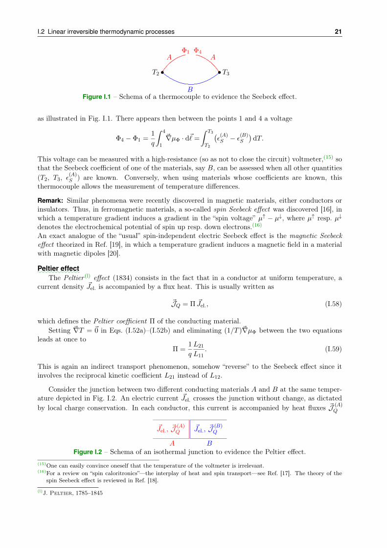
Figure I.1 – Schema of a thermocouple to evidence the Seebeck effect.
as illustrated in Fig. I.1. There appears then between the points 1 and 4 a voltage
Φ4 − Φ1 =1
q
∫ 4
1
~∇µΦ · d~=
∫ T3
T2
(ε(A)S − ε(B)
S
)dT.
This voltage can be measured with a high-resistance (so as not to close the circuit) voltmeter,(15) sothat the Seebeck coefficient of one of the materials, say B, can be assessed when all other quantities(T2, T3, ε
(A)S ) are known. Conversely, when using materials whose coefficients are known, this
thermocouple allows the measurement of temperature differences.
Remark: Similar phenomena were recently discovered in magnetic materials, either conductors orinsulators. Thus, in ferromagnetic materials, a so-called spin Seebeck effect was discovered [16], inwhich a temperature gradient induces a gradient in the “spin voltage” µ↑ − µ↓, where µ↑ resp. µ↓denotes the electrochemical potential of spin up resp. down electrons.(16)
An exact analogue of the “usual” spin-independent electric Seebeck effect is the magnetic Seebeckeffect theorized in Ref. [19], in which a temperature gradient induces a magnetic field in a materialwith magnetic dipoles [20].
:::::::::::::Peltier effect
The Peltier (l) effect (1834) consists in the fact that in a conductor at uniform temperature, acurrent density ~Jel. is accompanied by a flux heat. This is usually written as
~JQ = Π ~Jel., (I.58)
which defines the Peltier coefficient Π of the conducting material.Setting ~∇T = ~0 in Eqs. (I.52a)–(I.52b) and eliminating (1/T )~∇µΦ between the two equations
leads at once toΠ =
1
q
L21
L11. (I.59)
This is again an indirect transport phenomenon, somehow “reverse” to the Seebeck effect since itinvolves the reciprocal kinetic coefficient L21 instead of L12.
Consider the junction between two different conducting materials A and B at the same temper-ature depicted in Fig. I.2. An electric current ~Jel. crosses the junction without change, as dictatedby local charge conservation. In each conductor, this current is accompanied by heat fluxes ~J (A)
Q
A
~Jel., ~J(A)Q
B
~Jel., ~J(B)Q
Figure I.2 – Schema of an isothermal junction to evidence the Peltier effect.(15)One can easily convince oneself that the temperature of the voltmeter is irrelevant.(16)For a review on “spin caloritronics”—the interplay of heat and spin transport—see Ref. [17]. The theory of the
spin Seebeck effect is reviewed in Ref. [18].
(l)J. Peltier, 1785–1845

22 Thermodynamics of irreversible processes
and ~J (B)Q , which differ since Π(A) 6= Π(B). To ensure energy conservation, a measurable amount of
heatdQ
dt
∣∣∣∣Peltier
=(Π(A) −Π(B)
)Jel.
is released per unit time and unit cross-sectional area at the junction, with Jel. ≡∣∣ ~Jel.
∣∣. Note thatdQ/dt can be negative, which means that heat is actually absorbed from the environment at thejunction.
Comparing now the Seebeck coefficient (I.57) with the Peltier coefficient (I.59), one sees that therelation L21 = L12—which follows from Onsager’s reciprocal relation between LEN and LNE—leadsto
Π = εST, (I.60)
which is known as second Kelvin(m) relation (or sometimes second Thomson relation(17)).
Coming back to the fluxes (I.52a)–(I.52b) in the most general case of non-vanishing gradientsin temperature as well as in electrochemical potential, and eliminating (1/T )~∇µΦ between the tworelations, one find with the help of Eqs. (I.55), (I.59) and (I.60) the heat flux
~JQ = −κ ~∇T + εS T q ~JN . (I.61)
The first term corresponds to thermal conduction, the second to convection.
I.2.4 Linear transport phenomena in simple fluids
As last example of application of the formalism of linear Markovian thermodynamic processes,let us investigate transport phenomena in isotropic “simple” non-relativistic fluids, i.e. fluids madeof a single electrically neutral constituent, whose only species of (spherically symmetric) particleshave a mass m.
In such a system, the subsystems that coincide with the cells at the level of which local thermo-dynamic equilibrium and local extensive quantities are defined—the so-called fluid particles—canmove with respect to each other. The local momenta ~P (t,~r) of the various cells thus differ fromeach other, so that there is no global rest frame in which every local momentum would vanish. Thisconstitutes a new feature compared to the previous examples, and will require our determining theproper variables, as defined in some global reference frame, for the description of the system, beforewe can apply the generic ideas of linear Markovian processes.
Hereafter, the dependence of fields on time t and position ~r will generally not be written. Weshall use Cartesian coordinates labeled by indices i, j. . . running from 1 to 3, whose position willhave no meaning. The components of ~r will be denoted as xi.
::::::I.2.4 a
:::::::::::::::::::::::::::::::::::::::::::::::::::::::Extensive parameters, intensive quantities and fluxes
Each fluid cell is characterized by a set of local extensive variables, namely its total energy,particle number, and momentum. Both energy and momentum clearly depend on the referenceframe. On the one hand, we shall consider a fixed inertial frame R 0—corresponding to the framein which the observer who describes the fluid is at rest. In that frame, energy and momentum willbe denoted by E and ~P .
Alternatively, we shall also use an inertial frame R ~v which at time t moves with respect to R 0
with the same velocity ~v = ~v(t,~r) as the fluid particle located at position ~r. In that comoving frame,the fluid particle is momentarily at rest, so that R ~v will be referred to as comoving (local) rest frame,
(17)... which is historically more accurate, since William Thomson had not yet been ennobled as Lord Kelvin whenhe empirically found this relation in 1854.
(m)W. Thomson, Lord Kelvin, 1824–1907

I.2 Linear irreversible thermodynamic processes 23
where “local” conveniently emphasizes that at a given instant, the velocity takes different values atdifferent points, resulting in the existence of different comoving rest frames. In R ~v, the energy ofthe fluid cell reduces to its internal energy U while its momentum vanishes. Our first task is to findwhat are the conjugate intensive variables and fluxes in the fixed frame R 0.
Let M(t,~r) ≡ N(t,~r)m denotes the mass of fluid contained in the cell at position ~r at timet. E(t,~r) is then simply equal to the sum of the internal energy U(t,~r) and the kinetic energy~P (t,~r) 2/2M(t,~r) of the fluid particle. Thus, the characteristic extensive parameters of a cell in thefixed frame R 0 read
E = U +~P 2
2M, N, Pi, i ∈ 1, 2, 3, (I.62a)
with respective densities (amount per unit volume)
e+1
2ρ~v 2, n , ρ vi, (I.62b)
where ρ(t,~r) = mn(t,~r) is the mass density of the fluid.Writing that the entropy does not depend on the choice of the inertial frame in which it is
measured and equating its values in R 0 and R ~v, one finds the intensive variables conjugate to theextensive parameters (I.62), namely (see the derivation of YPi in Sec. I.1.3 a)
YE =1
T, YN = −µ~v
T= −
µ+ 12m~v
2
T, YPi = −vi
T(I.63)
respectively, where µ denotes the chemical potential in the comoving rest frame. Note that thetemperature does not depend on the reference frame.
The traditionally adopted variables in non-relativistic fluid dynamics are the mass density ρ(instead of n), the flow velocity ~v (instead of the momentum density) and the temperature T orequivalently the pressure P (instead of the energy density). The latter is given by the Gibbs–Duhem(n) relation
P = Ts− e+ µn . (I.64)
Since the right-hand side also reads Ts−(e+ 1
2ρ~v2)
+(µ+ 1
2m~v2)n , the pressure P keeps the same
value in every inertial frame.
Besides the densities (I.62b) and intensive variables (I.63), whose respective gradients are thevarious affinities, we still have to introduce the flux densities of the extensive parameters. Followingthe generic expansion (I.29a), these fluxes generally consist of a contribution depending on theaffinities, which describes the response of the system to a departure from equilibrium, and of affinity-independent equilibrium fluxes, which we shall now determine.
For that purpose, it is convenient to first establish the form of the equilibrium fluxes in thecomoving local rest frame R ~v before performing a Galilean transformation with velocity −~v toobtain the expressions in the fixed reference frame R 0.
In an equilibrated isotropic fluid at rest, invariance under rotations implies that the vectorialfluxes of internal energy and of particle number should vanish. Moreover, the momentum fluxdensity, which is a tensor of rank 2, must be proportional to the identity tensor, again to fulfillrotational symmetry, as argued in § I.2.2 a. To interpret the proportionality coefficient, one shouldrealize that the flux of the i-th component of linear momentum through a surface perpendicular tothe i-axis represents a normal force on that surface. In mechanical equilibrium, this force is balancedby the i-component of the force exerted by the remainder of the fluid on the surface element, i.e.in a fluid at rest through the hydrostatic pressure. All in all, one thus finds that the equilibriumfluxes in the comoving local rest frame are
~J eq.E
∣∣R~v
=~0, ~J eq.N
∣∣R~v
=~0, JJJ eq.~P
∣∣R~v
= P 111, (I.65)
(n)P. Duhem, 1861–1916
24 Thermodynamics of irreversible processes
where the latter identity can be expressed in term of components as (J eq.~P
)ij = P δij .
When performing the Galilean transformation with velocity −~v to the fixed reference frame R 0,two effects have to be taken into account. First, the transported quantities may be modified, as isthe case of energy density or momentum density. Secondly, a flux is defined as the quantity flowingper unit time through a motionless surface, and the motionless surfaces in both frames differ.
To consistently account for both these effects, one should first consider an infinitesimal Galileantransformation from a frame R ~v ′ with velocity ~v ′ (with respect to R 0) to a frame R ~v ′+d~v ′ withvelocity ~v ′ + d~v ′. In R ~v ′, the characteristic densities at a point moving with velocity ~v in R 0
take the values [cf. Eq. (I.62b)]
e+1
2ρ(~v −~v ′)2, n , ρ(vi − v′i).
Observed from R ~v ′+d~v ′, the densities at the same point become
e+1
2ρ(~v−~v ′−d~v ′)2 = e+
1
2ρ(~v−~v ′)2−ρ(~v−~v ′) ·d~v ′, n , ρ(vi−v′i−dv′i) = ρ(vi−v′i)−n mdv′i.
From the latter formulae, one deduces the variations of the densities in the infinitesimal Galileantransformation, namely respectively
d
(e+
1
2ρ ~w 2
)= ρ ~w · d~w, dn = 0, d
(ρ ~w)
= n m d~w,
where we have set ~w = ~v −~v ′ and accordingly d~w = −d~v ′.
Consider now the fluxes of the extensive quantities at the same point. Recognizing in theinfinitesimal variation of the energy density above the momentum density ρ ~w multiplied bythe velocity increment, one deduces that the change in energy flux due to the variation of thetransported energy density will involve the momentum flux, again multiplied by the velocityincrement. Similarly, the variation of momentum density involves the particle number density,so that the change in momentum flux will involve the flux of particle number.
On the other hand, the motion with velocity −d~v ′ in R ~v ′+d~v ′ of a surface which is motionlessin R ~v ′ contributes to any flux an amount given to first order in d~w by the product of thecorresponding density as measured in R ~v ′ with d~w
All in all, the differences between the values of the equilibrium fluxes as measured in R ~v ′+d~v ′
and R ~v ′ read
dJ eq.E,i =
3∑j=1
(Jeq.~P )ij dwj +
(e+
1
2ρ ~w 2
)dwi, d~J eq.
N = n d~w, d(Jeq.~P )ij = J eq.N,jm dwi + ρwi dwj .
These equations can be viewed as defining partial differential equations, which can be integratedfrom ~w = ~0 (i.e. from the local rest frame comoving with the fluid at velocity ~v) to ~w = ~v (thefixed frame), starting with known initial conditions at velocity ~w = ~0—namely the equilibriumfluxes (I.65). One first finds ~J eq.
N , which is then injected in the equations for (Jeq.~P )ij . Solvingthe latter, the result can be used in the equations for J eq.
E,i.
In the fixed reference frame R 0, the equilibrium fluxes read
~J eq.E =
(e+
1
2ρ~v 2 + P
)~v, ~J eq.
N = n~v,(Jeq.~P
)ij
= P δij + ρ vivj . (I.66)
These equilibrium fluxes have to be complemented with affinity-dependent terms, to yield the to-tal fluxes. For the sake of simplicity, we shall restrict ourselves to Markovian, memoryless transportprocesses.
By definition of the non-relativistic flow velocity as the average velocity of particles in the fluidcell under consideration, the flux of particle number does not receive any such extra term, and willalways remain equal to its equilibrium value, ~JN = ~J eq.
N .As a consequence (cf. the derivation above), the difference between the values of the momen-
tum flux components(J~P)ij
taken in the frames R 0 and R ~v is the same as for the corresponding
I.2 Linear irreversible thermodynamic processes 25
equilibrium fluxes, namely ρ vivj . The only dependence on any affinity in(J~P)ij
thus already af-fects its value in the local rest frame of the fluid, in which the diagonal tensor P δij becomes anaffinity-dependent tensor πππ with components πij called stress tensor .
Eventually, this stress tensor plays a role in the change of frame for the energy flux, with πππ ·~vreplacing P ~v. Additionally, one also has to allow for an affinity-dependent contribution ~JU to theenergy flux in the local rest frame. Altogether, one obtains the fluxes
~JE =
(e+
1
2ρ~v 2
)~v + ~JU +πππ ·~v, ~JN = n~v,
(J~P)ij
= πij + ρ vivj , (I.67)
where the functional dependences of ~JU and the stress tensor πππ on the various affinities depend onthe model under consideration, i.e. concretely on the specific fluid under study.
Remark: One can also show that angular momentum conservation implies that the stress tensor issymmetric.
::::::I.2.4 b
::::::::::::::::::::Conservation laws
Having obtained the fluxes in the fixed inertial frame R 0, we can now insert their expressionsand those of the densities (I.62b) in the general local balance equation (I.18a), where the source/sinkterm will vanish since energy, particle number and momentum are conserved.
Starting with particle number density, or equivalently—to respect the tradition—with the massdensity ρ = nm, the simple flux m~JN = ρ~v leads to the continuity equation
∂ρ
∂t+ ~∇ ·
(ρ~v)
= 0, (I.68)
which locally expresses mass conservation.In a second step, we can consider the balance equation for momentum, for the sake of simplicity
component by component. The momentum density ρ vi and flux J ij~Pgive for every i ∈ 1, 2, 3
∂(ρ vi)
∂t+
3∑j=1
∂
∂xj
(πij + ρ vivj
)= 0.
A simple calculation using the mass balance equation (I.68) to cancel two terms allows one to rewritethis relation as
ρ
[∂vi∂t
+(~v · ~∇
)vi
]+
3∑j=1
∂πij∂xj
= 0. (I.69)
Since the stress tensor component πij represents the amount of momentum in direction i flowingper unit time through a unit surface perpendicular to direction j, it equals according to Newton’s(o)
second law the i-th component of the force per unit area on a surface normal to the direction j.Following Newton’s third law, this equals the negative of the force per unit area exerted by theremainder of the fluid on the cell under study, so that this local balance equation actually expressesthe fundamental principle of Newtonian dynamics.
Eventually, the energy density (I.62b) and flux (I.67) yield for the local balance equation forenergy in the fixed reference frame
∂
∂t
(e+
1
2ρ~v 2
)+ ~∇ · ~JE =
∂
∂t
(e+
1
2ρ~v 2
)+
3∑i=1
∂
∂xi
[(e+
1
2ρ~v 2
)vi + ~JU +
3∑j=1
πijvj
]= 0.
To simplify this equation, one views 12ρ~v
2 as ρ times 12~v
2 and then differentiates with the usualproduct rule. The terms proportional to 1
2~v2 vanish thanks to the continuity equation (I.68). Those
(o)I. Newton, 1642–1727

26 Thermodynamics of irreversible processes
proportional to ρ can be rewritten with the help of the identity ~∇(
12~v
2)
=(~v ·~∇
)~v+~v×
(~∇×~v
), and
one recognizes the sum over i of ρvi multiplied with the term within square brackets in Eq. (I.69).A further application to the product rule leads then to
∂e
∂t+ ~∇ ·
(e~v + ~JU
)+
3∑i,j=1
πij∂vj∂xi
= 0. (I.70)
Interestingly, the kinetic energy density no longer appears in this equation, which can be interpretedas describing the change in the internal energy due to dissipation (~JU ) and to the work of forcesexerted on neighboring fluid cells (πij).
::::::I.2.4 c
::::::::::::::::::::::::::::::::::::::::::::::::::::::::Linear Markovian transport processes in a simple fluid
Let us now explicitly consider a model for the fluid, by assuming that the fluxes (I.67)—andmore precisely the flux ~JU and the stress tensor πππ—are linear functions of the affinities, i.e. of thefirst derivatives of the intensive variables (I.63) with respect to space coordinates. This assumptiondefines Newtonian fluids, which are those governed by the resulting dynamical laws derived fromEqs. (I.69) and (I.70).
In the linear regime, one only needs to introduce first-order kinetic coefficients Lab relating thefluxes to the affinities as in Eq. (I.31). Enumerating the former, the two vectors ~JN and ~JE andthe rank 2 tensor JJJ~P amount altogether to 15 components. Similarly, the gradients of the intensivevariables (I.63) also represent 15 different scalar fields, so that a naive approach would necessitate15× 15 kinetic coefficients Lab. Fortunately, the problem can be considerably simplified thanks tothe general principles of Sec. I.2.2 and to system-specific properties, resulting in a small number ofcoefficients.
A first important remark is that by definition of the flow velocity ~v, the particle-number flux ~JNalways remains equal to its equilibrium contribution ~J eq.
N = n ~v, irrespective of the affinities. Thismeans that all coefficients LNa vanish. Thanks to the Onsager relations, all reciprocal coefficientsLaN also vanish. Thus a gradient in chemical potential does not lead to any dissipation in a simplefluid: chemical potential plays no direct role in entropy production.(18)
Using the second consequence listed in Sec. I.2.2 of Curie’s symmetry principle applied toisotropic media, the vectorial flux (resp. affinity) for energy cannot couple to the affinity (resp.flux) for momentum, which is a tensor of rank 2. That is, the tensors of rank 3 coupling E and ~Pidentically vanish. All in all, this means that there is no indirect transport in a simple fluid.
According to the first of the consequences of isotropy given in Sec. I.2.2, the transport of energy—a scalar quantity—involves a tensor LLLEE of rank 2 proportional to the identity, i.e. effectively a singlekinetic coefficient LEE . To write down this relation explicitly, it is convenient to move to a restframe in which the fluid is locally at rest, so that the energy flux has a simple expression.
In the Galilean transformation from the fixed frame R 0 to the frame R ~v0 comoving with thefluid at point M0, where the fluid velocity at time t0 is ~v0, the position and velocity respectivelytransform according to ~r ′ = ~r−~v0(t− t0), which implies the identity of derivatives ∂/∂x′i = ∂/∂xi,and ~v ′(t,~r ′) = ~v(t,~r) − ~v0, where primed resp. unprimed quantities refer to R ~v0 resp. R 0. Sincetemperature is the same in all frames, the affinity conjugate to the energy is ~∇(1/T ), so that therelation between this affinity and the energy flux in the comoving rest frame reads
~JU = LEE~∇(
1
T
), (I.71a)
(18)A gradient in chemical potential, or equivalently in particle number density, at uniform temperature will lead viathe equations of state to a gradient in pressure P—cf. the example of an ideal gas—, which results in a macroscopicflow through Eq. (I.69). In turn, this motion will lead to dissipation due to the viscous effects described by thetransport coefficients η and ζ.

I.2 Linear irreversible thermodynamic processes 27
where LEE is as always nonnegative.In turn, the i-th component in R ~v0 of the affinity ~FPj is given by
∂
∂x′i
(−
v′jT
)∣∣∣∣t0,M0
=∂
∂xi
(− vj− v0,j
T
)∣∣∣∣t0,M0
= − 1
T
∂vj∂xi
∣∣∣∣t0,M0
,
where the term proportional to ∂(1/T )/∂xi vanishes since it multiplies vj−v0,j taken at time t0 andat the point M0. The remaining task is thus to express the components of stress tensor πππ, whichequals the momentum flux in the comoving local rest frame, as function of the derivatives ∂vk/∂xl.This necessitates a tensor LLL~P ~P of rank 4 with components Lijkl~P ~P
such that
πij =
3∑k,l=1
Lijkl~P ~P
∂vk∂xl
.
Invoking again the local isotropy of the fluid, this tensor can only be a linear combination of thethree rank-4 tensors invariant under rotations, namely those with (Cartesian) components δijδkl,δikδjl and δilδjk, with three respective kinetic coefficients.
As noted above, πππ must be symmetric (πij = πji) to ensure angular momentum conservation,so that the coefficients of δikδjl and δilδjk must be identical. Instead of considering πij as linearcombination of δijδkl and δikδjl + δilδjk, one traditionally—and equivalently—writes down a linearcombination of δijδkl and the traceless tensor 1
2
(δikδjl + δilδjk
)− 1
3δijδkl. Introducing the twonecessary non-negative coefficients L(1)
~P ~P, L(2)
~P ~P, the relation between the stress tensor components
and the affinities conjugate to momentum reads
πij = P δij −L
(1)~P ~P
T
3∑k,l=1
δijδkl∂vk∂xl−L
(2)~P ~P
T
3∑k,l=1
[1
2
(δikδjl + δilδjk
)− 1
3δijδkl
]∂vk∂xl
,
where we also included the equilibrium part P δij . With the help of the traceless symmetric tensorσσσ with components
σij ≡1
2
(∂vi∂xj
+∂vj∂xi
)− 1
3
(~∇ ·~v
)δij , (I.71b)
the stress tensor can be rewritten more concisely as
πππ = P 111−L
(1)~P ~P
T
(~∇ ·~v
)111−
L(2)~P ~P
Tσσσ (I.71c)
i.e. component-wise
πij = P δij −L
(1)~P ~P
T
(~∇ ·~v
)δij −
L(2)~P ~P
Tσij . (I.71d)
This relation and Eq. (I.71a) are the characteristic “constitutive equations” for a Newtonian fluid.
Let us now interpret the three kinetic coefficients LEE , L(1)~P ~P
and L(2)~P ~P
in terms of more traditionaltransport coefficients.
First, Eq. (I.71a) is naturally reminiscent of Fourier’s law
~JU = −κ~∇T with κ =LEET 2
(I.72)
like in the case of an insulator [Eq. (I.37a)]. LEE is thus related to the heat conductivity, which isnonnegative, as it should be.
As was already mentioned, πij is the i-component of the force per unit area acting on a surfacenormal to the j-direction. Phenomenologically, this force per unit area is related to the gradientalong direction j of the i-th component of velocity through Newton’s law of viscosity(19)
(19)This law is defined for a fluid flowing uniformly along the i-direction, so that the velocity only depends on xj ,which ensures that both ∂vi/∂xi—and thereby ~∇ ·~v—and ∂vj/∂xi vanish.
28 Thermodynamics of irreversible processes
πij = −η dvidxj
, (I.73)
with η the shear viscosity of the fluid. Identifying this empirical law with relation (I.71d) for i 6= jyields
η =L
(2)~P ~P
2T. (I.74)
Eventually, the parameter L(1)~P ~P
is related to the transport parameter referred to as volumeviscosity (or at times second viscosity or bulk viscosity(20)) ζ, which only plays a role in compressibleflows (~∇ ·~v 6= 0), in particular in the damping of sound waves. To obtain the proper form for theequation of motion of a compressible flow, one must set
ζ =L
(1)~P ~P
T. (I.75)
With Eqs. (I.74) and (I.75), the stress tensor component (I.71c) becomes
πππ = P 111− ζ(~∇ ·~v
)111− 2ησσσ. (I.76)
Rewriting Eqs. (I.69) and (I.70) in the linear regime in which the internal energy and momentumfluxes are respectively given by Eqs. (I.72) and (I.76), one obtains in the case of position-independentviscosity coefficients the Navier (p)–Stokes(q) equation
ρ
[∂~v
∂t+(~v · ~∇
)~v
]= −~∇P + η
[4~v +
1
3~∇(~∇ ·~v
)]+ ζ~∇
(~∇ ·~v
)(I.77)
and the energy balance equation
∂
∂t
(e+
1
2ρ~v 2
)+ ~∇ ·
(e+
1
2ρ~v 2 + P
)~v
− η[(~v · ~∇
)~v + ~∇
(~v 2
2
)− 2
3~v(~∇ ·~v)
]− ζ~v
(~∇ ·~v)− κ~∇T
= 0.
(I.78)
::::::I.2.4 d
::::::::::::::::::::Entropy production
To conclude this application of the thermodynamics of linear irreversible processes to simplefluids, we can write down the balance equation for entropy (I.20).
For that purpose, we first need the expression of the entropy flux density. Using the generalformula (I.22) in the comoving local rest frame R ~v, in which ~JN = ~0 and Y~P = ~0 since both are inthe general case proportional to the fluid velocity, yields
(~JS)R~v =1
T~JU . (I.79a)
Transforming back to the fixed frame R 0, the entropy density s is invariant, so that the entropyflux only changes because surfaces at rest in R ~v are now moving:
~JS =1
T~JU + s~v (I.79b)
(20)Some authors, as e.g. in Ref. [21], reserve the name “bulk viscosity” to the combination ζ + 23η. The lack of unity
in the terminology shows how little this coefficient has actually been studied!(p)C.L. Navier, 1785–1836 (q)G. G. Stokes, 1819–1903

I.2 Linear irreversible thermodynamic processes 29
Inserting in the general formula for the entropy production (I.30) the fluxes (I.67) from whichone subtracts their equilibrium values (I.66) with the corresponding affinities, one finds(21)
σS = ~∇(
1
T
)· ~JU +
3∑i,j=1
(− 1
T
∂vj∂xi
)(πij − Pδij
). (I.80)
In the linear approximation where the fluxes are respectively given by Eqs. (I.72) and (I.76),this becomes
σS = κT 2
[~∇(
1
T
)]2
+3∑
i,j=1
(− 1
T
∂vj∂xi
)[−2ησij − ζ
(~∇ ·~v
)δij
].
The rightmost term between square brackets is symmetric under the exchange of i and j, so that onecan replace ∂vj/∂xi in front by half of the symmetrized version, i.e. according to definition (I.71b)by σij + 1
3(~∇ ·~v)δij . Canceling out the minus signs, one thus has
σS = κT 2
[~∇(
1
T
)]2
+1
T
3∑i,j=1
[σij +
1
3
(~∇ ·~v
)δij
][2ησij + ζ
(~∇ ·~v
)δij
].
The remaining product can then be expanded. Multiplying a rank 2 tensor by δij and taking thesum over i and j amounts to taking the trace of the tensor. Since σij is traceless, the productsσijδij yield 0, while δijδij gives 3. In the end, there remains
σS = κT 2
[~∇(
1
T
)]2
+ζ
T
(~∇ ·~v
)2+
2η
T
3∑i,j=1
(σij)2. (I.81)
Since the three transport coefficients κ, η and ζ are nonnegative, the entropy production rate isalways positive—as it should be.
Bibliography for Chapter I• Blundell & Blundell, Concepts in thermal physics [22], chapter 34.
• Callen, Thermodynamics and an introduction to Thermostatistics [8], chapter 14.
• de Groot & Mazur, Non-equilibrium thermodynamics [1], chapters II–IV, VI, XI §1&2, XII§1.
• Le Bellac, Mortessagne & Batrouni, Equilibrium and non-equilibrium statistical thermodynam-ics [9], chapter 6.
• Pottier, Nonequilibrium statistical physics [6], chapter 2.
(21)This is most obvious in the comoving frame, holds however in a general frame.
CHAPTER II
Distributions of statistical mechanics
The purpose of Statistical Mechanics is to explain the thermodynamic properties of macroscopicsystems starting from underlying microscopic models—possibly based on “first principle” theories.In this chapter, we shall first argue that such an approach in practice inevitably involves probabilitiesto be predictive (Sec. II.1). The specific modalities of the implementation of probabilities are thenpresented for both classical (Sec. II.2) and quantum mechanical (II.3) systems. We shall on purposeintroduce descriptions that are very parallel to each other, which will in following chapters allowus to treat some problems only in the quantum mechanical framework and argue that the samereasoning could have been adopted in a classical setup, and reciprocally. Eventually, Sec. II.4deals with the missing information arising from the probabilistic nature of the description, and itsquantitative measure.
II.1 From the microscopic scale to the macroscopic world
II.1.1 Orders of magnitude and characteristic scales
The notion of a macroscopic system and the related variables are usually understood to applyto a system whose characteristic scales are close to (or much larger than) the scales relevant fora human observer, namely typical length scales of 1mm – 1m or larger, durations of 1 s, kineticenergies of 1 J, and so on.
In opposition, microscopic scales—at which the laws of the dynamics of point particles ap-ply(22)—are rather understood to refer to atomic or molecular scales. For instance, the typical dis-tance between atoms or molecules—collectively called “particles” in the following for brevity(22)—ina solid or a gas is about 10−10 to 10−8 m respectively, so that 1 cm3 of solid resp. gaseous phaseconsists of N ≈ 1024 resp. 1019 particles. The typical microscopic energy scale is the electron-volt,where 1 eV is 1.6×10⁻¹⁹ J, while the typical durations range from ca. 10−15 s [= ~/(1 eV)] to 10−9 s(typical time interval between two collisions of a particle in a gas under normal conditions).
Remarks:
∗ In the case of the usual application of the concepts of Statistical Physics discussed above, theinteraction between microscopic degrees of freedom is mostly of electromagnetic nature. The dis-tances between particles are too large for the strong or weak interactions to play a role, whilethe masses remain small enough, to ensure that gravitational effects are negligible with respect toelectromagnetic ones—unless of course when investigating astrophysical objects.
∗ The methods of Statistical Physics are also sometimes applied in circumstances in which theparticle number is much smaller than above. For instance, the 103–104 particles emitted in high-energy collisions of heavy nuclei are often considered as forming a statistical system—even worse, asystem possibly in local thermodynamic equilibrium.(22)This generic denomination “(point) particles” does not necessarily involve a description in terms of particles. It
is rather a convenient shorthand expression for “elementary degrees of freedom”, which may possibly actually bedescribed by some quantum field theory.
II.2 Probabilistic description of classical many-body systems 31
∗ At the other end of the length spectrum, some astrophysical simulations treat stars or evengalaxies as pointlike objects constituting the “microscopic” scale in the respective descriptions ofgalaxies or galaxy clusters.
II.1.2 Necessity of a probabilistic description
A typical macroscopic system consists in general of a large number of degrees of freedom, whichobey microscopic laws. Theoretically, one could think of simulating the evolution of such a system—say for instance of 1023 particles—on a computer. The mere storage of the positions and momentaat a given instant t0 of so many particles, coding them as real numbers in simple precision (4 Bytes),already requires about 1012 hard disks with a capacity of 1 TB! This represents only the first step,since one should still solve the equations of motion for the particles. . . As of late 2014, the mostextensive simulations of molecular dynamics study the motion of N . 107 particles over a timeduration . 1µs, i.e. for about 106–108 time steps.(23),(24)
In addition, the dynamical equations of such a many-body system are characterized by theirsensitivity to the initial conditions, which grows with increasing particle number. Thus, two trajec-tories in the phase space of a classical system that correspond to initial conditions which only differby an infinitesimal distance ε might after a duration t be about ε eλt away from each other withsome Lyapunov (r) exponent λ > 0; that is, an originally infinitesimal error grows exponentially. Thesystem is then chaotic and any prediction regarding individual particles quickly become hazardous.
As a consequence, one has to abandon the idea of a purely deterministic microscopic descriptioneven in the case of a classical system, and adopt a new approach. Instead of attempting to describethe exact microscopic state, or more briefly microstate, of a system at a given instant, one mustrather investigate the probability to find the system in a given microstate. In that approach, onemust characterize the system through macroscopic quantities, defining a macrostate.
Such a macroscopic observable usually results from a sum over many particles of microscopicquantities, and is often defined as the expectation value of the sum or of the arithmetic mean.Thanks to the central limit theorem (Appendix B.5) the fluctuations of the sum about this expec-tation value are of relative magnitude 1/
√N , i.e. very small when N & 1020, so that the observable
is known with high accuracy.In practice, the phenomenological laws relating such macroscopic observables have been ob-
tained by repeating several measurements, the results of which have been averaged to get rid ofexperimental uncertainties. For instance, establishing the local form of Ohm’s law (I.41b) relieson performing many measurements of the electrostatic field in the conductor and of the resultingelectric current density, and the obtained law should rather read 〈 ~Jel.〉 = σel.〈 ~E 〉, which describesthe actual procedure better than the traditional form (I.41b), and again emphasizes the need for astatistical approach.
II.2 Probabilistic description of classical many-body systemsIn the previous section, it has been argued that the description of a macroscopic physical sys-tem should be based on a statistical approach. We now discuss the practical introduction of thecorresponding probabilities in the microscopic formalism of classical mechanics.(23)An explicit example is the simulation of the motions of 6.5 million atoms for about 200 ns within a multi-time-step
technique involving steps of 0.5, 2 and 4 fs for various “elementary processes” [23].(24)The current tendency is not towards increasing these numbers by brute force, but rather to use “multiscale
approaches” in which part of the large scale phenomena are no longer described microscopically, but using macro-scopic variables and evolution equations.
(r)A. Lyapunov, 1857–1918

32 Distributions of statistical mechanics
After recalling the basics of the phase-space based formalism for exactly known classical sys-tems (Sec. II.2.1), we introduce the notion of a probability density on phase space to account forincomplete knowledge of the exact microscopic state of a system with a given finite number of con-stituents (Sec. II.2.2). We next derive the evolution equations governing the dynamics of that density(Sec. II.2.3) and of observables (Sec. II.2.4). Eventually, we shortly mention the generalization tosystems whose particle number is not fixed (Sec. II.2.5).
The purpose in the following is not only to present the necessary statistical concepts, but wealso aim at developing a formalism that is close enough to that introduced in Sec. II.3 for quantum-mechanical systems—as will e.g. be reflected in formally identical evolution equations for the proba-bility densities or the observables [see Eqs. (II.12) and (II.28) or (II.16) and (II.38)]. In this sectionthis might first seem to entail unnecessary complications; yet it will later turn out to be useful.
II.2.1 Description of classical systems and their evolution
::::::II.2.1 a
::::::::::::::::::::::::::::State of a classical system
Consider an isolated classical system of N identical pointlike particles in three-dimensionalEuclidean space. The microstate of the system at a time t is entirely characterized by the 3N spacecoordinates of the particles q1, . . . , q3N and their 3N conjugate momenta p1, . . . , p3N . Together,these positions and momenta constitute a point in a 6N -dimensional space, the phase space (orΓ-space) of the system. Reciprocally, each point in this phase space corresponds to a possiblemicrostate of the system.
For such a classical system, a measurable quantity—or (classical) observable—is defined as aphase-space function ON (qi, pi) of the 6N variables. We shall only consider observables withoutexplicit time dependence, i.e. the mathematical function ON remains constant over time.
Remark: If the particles are not pointlike, but possess internal degrees of freedom that can bedescribed classically, then the formalism further applies taking into account these extra degrees offreedom. The qi and pi are then generalized positions and momenta.
::::::II.2.1 b
:::::::::::::::::::::::::Evolution of the system
The time evolution of the system is represented in Γ-space by the trajectory (qi(t), pi(t))of the representative point, which describes a succession of microstates. The “velocity” tangentto this trajectory is the 6N -dimensional vector u whose 6N components are the time derivativesqi(t), pi(t).
The dynamics of the system—or equivalently, of the representing point in Γ-space—is fullydetermined by specifying the time-independent Hamilton(s) functionHN (qi, pi). More precisely,the trajectory (qi(t), pi(t)) is governed by the Hamilton equations
qi(t) ≡dqi(t)
dt=∂HN
∂pi= qi, HN,
pi(t) ≡dpi(t)
dt= −∂HN
∂qi= pi, HN, i = 1, . . . , 3N,
(II.1)
where the derivatives of the Hamilton function, and accordingly the Poisson brackets, are to becomputed at the point in Γ-space where the system sits at time t, i.e. at (qi = qi(t), pi = pi(t))for 1 ≤ i ≤ 3N . The Poisson(t) bracket of two functions f , g defined on phase space is given by(25)
f, g ≡3N∑i=1
(∂f
∂qi
∂g
∂pi− ∂f
∂pi
∂g
∂qi
), (II.2)
wherethe arguments of the functions and their derivatives have been dropped for the sake of brevity.(25)The sign convention for Poisson brackets is not universal... The choice taken here is the same as in Goldstein [24]
or Arnold [25], while Landau & Lifshitz adopt the opposite convention [26].(s)W. R. Hamilton, 1805–1865 (t)S. Poisson, 1781–1840
II.2 Probabilistic description of classical many-body systems 33
It is important to realize that the Hamilton equations are fully deterministic once the Hamiltonfunction is fixed: given an initial condition (qi(0), pi(0)), the microstate at time t is uniquelydetermined by Eqs. (II.1). Accordingly, there is only a single trajectory through each individualpoint of the Γ-space, so that the notation u(qi, pi) is non-ambiguous.
II.2.2 Phase-space density
In a many-body system, the precise microstate corresponding at a given time to determinedmacroscopic properties—for example, given volume, particle number N and energy—is not exactlyknown. As a consequence, one introduces a probability distribution ρN (t, qi, pi) on the Γ-space,the N -particle phase space density , which is as always nonnegative and normalized to unity
ρN(t, qi, pi
)≥ 0 ∀qi, pi and
∫ΓρN(t, qi, pi
)d6NV = 1, (II.3)
where the integral runs over the whole Γ-space. ρN (t, qi, pi) d6NV is the probability that themicrostate of the system at time t lies in the infinitesimal volume element d6NV around the point(qi, pi). The volume element d6NV should represent a uniform measure on the phase space, sothat
d6NV = CN
3N∏i=1
dqi dpi, (II.4a)
with CN a normalization factor. A possible choice for the latter—and admittedly the most natural—is simply CN = 1. Another choice, which is less natural yet allows one to recover classical mechanicsas a limiting case of quantum mechanics, is to adopt for a system of N indistinguishable particlesthe measure
d6NV =1
N !
3N∏i=1
dqi dpi2π~
, (II.4b)
with ~ the reduced Planck(u) constant. A further advantage of this choice is that d6NV is dimen-sionless, and thus the probability density ρN as well.
Remark: To interpret probabilities as counting the number of favorable cases among all possibleoutcomes, Gibbs introduced the idea of mentally considering many copies of a system—which alto-gether constitute a statistical ensemble—, where the copied systems all have the same macroscopicproperties, although the corresponding microstates differ.
After having introduced the phase space density ρn, the position in Γ-space (qi(t), pi(t))at time t can be viewed as a 6N -dimensional random variable. Again, the microstate at t is notrandom if (qi(t= 0), pi(t= 0)) is known, but randomness enters due to our knowledge of theinitial condition only on a statistical basis.
In turn, the value taken by an observable ON (qi, pi) for a given system—corresponding toa given trajectory in Γ-space—at time t, namely
ON (t) ≡ ON(qi=qi(t), pi=pi(t)
), (II.5)
is also a random variable, whose momenta are given by the usual formulae (see Appendix B). Forinstance, the average value at time t is
〈ON (t)〉t =
∫ΓON(qi, pi
)ρN(t, qi, pi
)d6NV (II.6a)
and the variance readsσ2ON
(t) =⟨ON (t)2
⟩t− 〈ON (t)〉2t , (II.6b)
(u)M. Planck, 1858–1947
34 Distributions of statistical mechanics
where the subscript t emphasizes the use of the phase-space density at time t in computing theexpectation value.
Remark: Even it has been assumed that the observable On has no explicit time dependence, themoments of the observable do depend on the instant at which they are computed.
II.2.3 Time evolution of the phase-space density
Consider a fixed volume V in the phase space Γ, and let N (t) denote the number of particlesinside that volume at time t. We can write the rate of change of this number in two alternativeways.
Expressing first the number of particles with the help of the phase-space density
N (t) = N
∫VρN(t, qi, pi
)d6NV , (II.7)
one finds that N (t) changes because the phase-space density is evolving in time:
dN (t)
dt= N
∫V
∂ρN(t, qi, pi
)∂t
d6NV . (II.8)
Alternatively, one can view the change in N (t) as due to the flow of particles through the surface∂V enclosing the volume V . Let en(qi, pi) denote the unit vector normal to ∂V at a givenpoint, oriented towards the outside of V , and u(qi, pi) be the velocity-vector tangent to thetrajectory passing through the point (qi, pi). One then has
dN (t)
dt= −N
∫∂VρN(t, qi, pi
)u(qi, pi) · en(qi, pi) d6N−1S.
The divergence theorem transforms the surface integral over ∂V into a volume integral over V
dN (t)
dt= −N
∫V∇ ·
[ρN(t, qi, pi
)u(qi, pi)
]d6NV , (II.9)
with ∇ the 6N -dimensional gradient in phase space.Equating Eqs. (II.8) and (II.9) and arguing that they hold for an arbitrary volume V , one
obtains the local conservation equation in Γ-space (for the sake of brevity, the variables are notwritten)
∂ρN∂t
+∇ ·(ρNu
)= 0. (II.10a)
The divergence in the left-hand side can be rewritten as
∇ ·(ρNu
)=
3N∑i=1
∂
∂qi
(ρN qi
)+
3N∑i=1
∂
∂pi
(ρN pi
)=
3N∑i=1
(∂ρN∂qi
qi +∂ρN∂pi
pi
)+
3N∑i=1
(∂qi∂qi
+∂pi∂pi
)ρN .
With the help of the Hamilton equations (II.1) this gives the Liouville(v) equation(26)
∂ρN∂t
+
3N∑i=1
(∂ρN∂qi
∂HN
∂pi− ∂ρN
∂pi
∂HN
∂qi
)=∂ρN∂t
+ρN , HN
= 0. (II.10b)
(26)Here it is implicitly assumed that the Hamilton function HN is sufficiently regular—namely that the second partialderivatives are continuous—so as to have the identity
∂qi∂qi
=∂
∂qi
∂HN∂pi
=∂
∂pi
∂HN∂qi
= −∂pi∂pi
.
(v)J. Liouville, 1809–1882

II.2 Probabilistic description of classical many-body systems 35
Introducing the Liouville operator (or Liouvillian) L defined by(27)
iL ≡3N∑i=1
(∂HN
∂pi
∂
∂qi− ∂HN
∂qi
∂
∂pi
)=· , HN
, (II.11)
where the dot stands for the phase-space function on which the operator acts, Eq. (II.10b) can berecast in the form
∂ρN∂t
+ iLρN = 0. (II.12)
Like the Hamilton function, the Liouville operator for an isolated system is time-independent,which allows one to formally integrate the Liouville equation as
ρN (t, qi, pi) = e−iLt ρN(t=0, qi, pi
), (II.13)
with ρN(t= 0, qi, pi
)the initial phase-space density at t = 0. To account for this result, e−iLt
is sometimes called time propagation operator .
Remarks:
∗ An equivalent formulation of the Liouville equation, which follows from Eq. (II.10a) under con-sideration from the Hamilton equations, which yield ∇ · u = 0 (see the identity in footnote 26),is
∂ρN∂t
+ u ·∇ρN =DρNDt
= 0, (II.14)
withD
Dt≡ ∂
∂t+ u ·∇ the material (or convective, substantial , hydrodynamic) derivative.
∗ Equations (II.10b), (II.12) or (II.14) represent the Eulerian(w) viewpoint on the Liouville equa-tion. Alternatively, one can adopt the Lagrangian(x) viewpoint and follow individual trajectories inΓ-space in their motion.
More precisely one should consider a continuous distribution of microstates, to ensure that thephase-space volume they occupy at a given instant has a non-zero measure. This collection ofΓ-space points is then sometimes referred to as a phase(-space) fluid , and its motion—along thecorresponding trajectories—as the flow of that fluid.
The corresponding statement of the Liouville equation, which is then known as Liouville theorem,is the following:
The volume in phase space occupied by a collection of microstates for a systemobeying the Hamilton equations of motion remains constant in time. (II.15)
That is, the volume of the phase-space fluid is an integral constant of the motion. Accordingly, oneoften states that the flow of trajectories in phase space is incompressible.
∗ The Liouville equation (II.10b) or (II.12) shows that if the phase-space density ρN is a functionof the Hamilton function HN , then it is stationary. This is for instance the case at equilibrium(28),but not only.
(27)The conventional—and not universally adopted—factor i has the advantage that it leads to results that are easilycompared to the quantum-mechanical ones.
(28). . . in which case ρN ∝ e−βHN with β ≡ 1/kBT .
(w)L. Euler, 1707–1783 (x)J.-L. Lagrange, 1736–1813
36 Distributions of statistical mechanics
II.2.4 Time evolution of macroscopic observables
As mentioned above, classical observables are defined as time-independent functions on phasespace, which however acquire an implicit time dependence when computed along the Γ-space tra-jectory of a system, see Eq. (II.5). Differentiating ON (t) with the chain rule gives
dON (t)
dt=
3N∑i=1
[∂ON∂qi
qi(t) +∂ON∂pi
pi(t)
],
where the derivatives with respect to the Γ-space coordinates are taken at the point (qi(t), pi(t))along the system phase-space trajectory. Under consideration of the Hamilton equations (II.1), thisbecomes
dONdt
=3N∑i=1
(∂ON∂qi
∂HN
∂pi− ∂ON
∂pi
∂HN
∂qi
)=ON , HN
= iLON , (II.16)
where we have used the definitions of the Poisson bracket (II.2) and of the Liouville operator (II.11).Invoking again the time-independence of the Liouville operator, the differential equation (II.16)
can formally be integrated asON (t) = eiLtON (t=0), (II.17)
with ON (t=0) the initial value of the observable at time t = 0.The expectation value of the observable obtained by averaging over the initial conditions at
t = 0 then reads
〈ON (t)〉0
=
∫ΓρN(t=0, qi, pi
)ON (t) d6NV
=
∫ΓρN(t=0, qi, pi
)eiLtON (t=0) d6NV . (II.18)
Alternatively, one can directly average ON (qi, pi) with the phase-space density at time t, asdone in Eq. (II.6a):
〈ON (t)〉t =
∫ΓON(qi, pi
)ρN(t, qi, pi
)d6NV .
Using Eq. (II.13), this becomes
〈ON (t)〉t =
∫ΓON(qi, pi
)e−iLt ρN
(t=0, qi, pi
)d6NV . (II.19)
Both points of view actually yield the same result— i.e. 〈ON (t)〉0
= 〈ON (t)〉t—, which meansthat one can attach the time dependence either to the observables or to the phase-space density,which stands for the macrostate of the system.
This equivalence can be seen by computing the time derivatives of Eqs. (II.18)—which is theaverage of Eq. (II.16) over initial positions—and (II.19). Replacing the Liouville operator byits expression in terms of the Hamilton function, and performing a few partial integrations tohandle the Poisson brackets, one finds that these time derivatives coincide at any time t. Sincethe “initial” conditions at t = 0 also coincide, the identity of 〈ON (t)〉
0and 〈ON (t)〉t follows.
Remark: More generally, the identity∫Γg∗(qi, pi)Lh(qi, pi) d6NV =
∫Γ(Lg)∗(qi, pi)h(qi, pi) d6NV ,
holds for every pair of phase-space functions g(qi, pi) and h(qi, pi) which vanish sufficientlyrapidly at infinity, where f∗ denotes the complex conjugate function to f . Recognizing in the phase-
II.3 Probabilistic description of quantum mechanical systems 37
space integral of g∗h an inner product 〈g, h〉, the above identity can be recast as 〈g,Lh〉 = 〈Lg, h〉,which expresses the fact that the Liouville operator is Hermitian for the inner product. In turn, theoperators e±itL , which govern the evolution of the density ρN or of observables ON (t), are unitaryfor this product, i.e. 〈g, e−itLh〉 = 〈eitLg, h〉 or equivalently:∫
Γg(qi, pi) e−itLh(qi, pi) d6NV =
∫Γ
[eitLg(qi, pi)
]h(qi, pi) d6NV . (II.20)
II.2.5 Fluctuating number of particles
Until now, we have assumed that the particle number N is exactly known. It is however oftennot the case, so that N also becomes a random variable, with a discrete probability distribution.
The formalism can easily be generalized to accommodate for this possibility. The new phasespace is the union—if one wants to be precise, the direct sum—of the individual N -particle phasespaces for every possible value of N , i.e. for N ∈ N.(29) The probability density ρ on this phase spaceconsists of (the tensor product of) densities ρN proportional to the respective N -particle densitiesρN , yet normalized so that
πN =
∫ρN (t, qi, pi) d6NV
represents the probability to have N particles in the system at time t.
An observable O is also defined as a tensor product of functions ON on each N -particle phasespace, with the expectation value
〈O(t)〉t =
∞∑N=0
∫ON (qi, pi) ρN (t, qi, pi) d6NV .
II.3 Probabilistic description of quantum mechanical systemsIn the “classical” formalism of quantum mechanics, the state of a system—if it is exactly known, inwhich case it is referred to as a pure state—is described by a normalized vector |Ψ〉 of a Hilbert(y)
space H . In turn, observables are modeled by Hermitian operators O(t) on H .In this section, we recall the basics of the formalism for the description of macroscopic quantum
systems based on the density operator (Sec. II.3.1). We then discuss the time evolution of the latter(Sec. II.3.2) as well as that of the expectation values of observables (Sec. II.3.3). Eventually, weconsider the case in which the Hamilton operator governing the evolution of the system can besplit into two terms, namely a time-independent one and a time-dependent “perturbation” that isswitched on at some initial instant (Sec. II.3.4).
II.3.1 Randomness in quantum mechanical systems
::::::II.3.1 a
:::::::::::::::::::::::::::::Randomness in pure states
Experimentally, this pure state is entirely determined by the results of measurements of quanti-ties associated with the operators of a complete set of commuting observables, where the latter areHermitian linear operators on H .
In quantum mechanics, the result of a measurement performed on a pure state |Ψ〉 might alreadybe a random variable, in case |Ψ〉 is not an eigenstate of the observable O associated to the measured
(29)The case N = 0 has to be considered as well, corresponding here to a 0-dimensional phase space reduced to asingle point.
(y)D. Hilbert, 1862–1943

38 Distributions of statistical mechanics
quantity. In that case, repeated measurements will give the expectation value of the observableaccording to
〈O〉 = 〈Ψ| O |Ψ〉. (II.21)
::::::II.3.1 b
:::::::::::::::::::::::::::::::Randomness in mixed states
In realistic cases, the microstate |Ψ〉 of a macroscopic system is not exactly determined. Instead,one only knows that the system can be with probability p1 in microstate |Ψ1〉, with probability p2
in another microstate |Ψ2〉, and so on, where the states |Ψ1〉, . . . , |Ψm〉, . . . are normalized, but notnecessarily orthogonal, while the probabilities p1, . . . , pm, . . . satisfy
pm ≥ 0 ∀m and∑m
pm = 1.
One speaks then of a statistical ensemble or statistical mixture of states, or in short—and somewhatmisleadingly—of a mixed state.
Remark: A mixed state should not be confused with a linear combination of states. In the lattercase, the system is still in a pure state, corresponding to a single vector of the Hilbert space.
The expectation value of an observable for a system in a mixed state is the weighted sum of theexpectation values in the pure states:
〈O〉 =∑m
pm〈Ψm| O |Ψm〉. (II.22a)
To express such expectation values in a convenient way, one introduces the density operator(also called statistical operator or density matrix )(30)
ρ =∑m
pm |Ψm〉〈Ψm| . (II.22b)
One then has the identity〈O〉 = Tr
(ρ O), (II.22c)
where Tr denotes the trace of an operator.
Using the matrix elements ρij and Oij of ρ and O in an arbitrary basis |φj〉 of H , as well astwo decompositions of the identity, one finds at once
〈O〉 =∑i,j
∑m
pm〈Ψm |φi〉〈φi| O |φj〉〈φj |Ψm〉 =∑i,j
ρijOji = Tr(ρ O). 2
Remarks:∗ The probabilities p1, . . . , pm, . . . are clearly the eigenvalues of the density operator ρ.
∗ The density-operator formalism easily accommodates the description of both mixed states andpure states. Thus, a microstate |Ψ〉 ∈ H can be equivalently represented by the density operatorρ = |Ψ〉〈Ψ| acting on the Hilbert space H .
Properties of the density operator
1. ρ is Hermitian: ρ† = ρ.As a consequence, the expectation value of every observable is real.
The proof follows from the hermiticity of O and the invariance of the trace under cyclicpermutations: 〈O〉∗ =
[Tr(ρ O)]∗
= Tr(O†ρ†
)= Tr
(O ρ)
= Tr(ρ O)
= 〈O〉. 2
2. ρ is positive: ∀ |φ〉 ∈H , 〈φ| ρ |φ〉 ≥ 0.Thus, the expectation value of every positive operator is a positive number.
(30)See e.g. Refs. [27] chapter EIII or [3] § 5.

II.3 Probabilistic description of quantum mechanical systems 39
3. ρ is normalized to unity: Tr ρ = 1.This means that the expectation value of the identity equals 1.
The whole information on the system is encoded in its density operator ρ. If one considers itsmatrix elements ρij in an arbitrary basis |φj〉, then each diagonal element, called population, ρiiis the probability to find the system in state |φi〉.The off-diagonal elements ρij with i 6= j are called coherences, and represent an information on thequantum-mechanical correlations between the possible states |φi〉 and |φj〉 of the system, which isabsent in a classical description.
Remark: From the positivity of the density operator follows the positivity of each of its minors ina given basis, in particular the inequality ρiiρjj − ρijρji ≥ 0. Since ρji = ρ∗ij , one sees that thecoherence between two states can only be non-zero when the populations of these states do notvanish.
::::::II.3.1 c
:::::::::::::::::::::::::::::::::Fluctuating number of particles
To account for possible fluctuations in the number of particles in a quantum-mechanical system,one introduces the Fock (z) space, that is the Hilbert space H defined as direct sum of the Hilbertspaces HN corresponding to the N -particle problems, including the one-dimensional space H0
spanned by the vacuum state |0〉 describing the absence of particles.The density operator ρ then simply acts on this Fock space and allows one to compute the
expectation value of an observable—represented as an Hermitian operator on H —through theusual formula (II.22c).
II.3.2 Time evolution of the density operator
Consider a macroscopic system, with the (possibly time-dependent) Hamilton operator H(t).Starting from the Schrödinger(aa) equation
i~∂|Ψ(t)〉∂t
= H(t)|Ψ(t)〉, (II.23)
which holds for every pure state |Ψm〉 in which a statistical mixture can be, one finds that the timeevolution of the density operator ρ(t) is governed by the Liouville–von Neumann(ab) equation
∂ρ(t)
∂t=
1
i~[H(t), ρ(t)
], (II.24)
where the square brackets denote the commutator of two operators.
Considering the Hermitian conjugate equation to the Schrödinger equation, one finds∂ρ(t)
∂t=∑m
pm
(∂|Ψm〉∂t〈Ψm| + |Ψm〉
∂〈Ψm|∂t
)=∑m
pm
(1
i~H|Ψm〉〈Ψm| +
1
−i~|Ψm〉〈Ψm| H
),
which can be recast as Eq. (II.24). 2
The solution of this differential equation for a given initial condition ρ(t0) at some time t = t0can be expressed in terms of the time-evolution operator U(t, t0).(31) Recall that the latter evolvespure states of the system—described as vectors of H (t)—between the initial time t0 and time t
|Ψ(t)〉 = U(t, t0)|Ψ(t0)〉. (II.25a)
As such, the time-evolution operator is solution to the first-order differential equation
i~∂
∂tU(t, t0) = H(t) U(t, t0), (II.25b)
(31)See e.g. Ref. [27] chapter FIII.(z)V. A. Fock (or Fok), 1898–1974 (aa)E. Schrödinger, 1887–1961 (ab)J. von Neumann, 1903–1957

40 Distributions of statistical mechanics
with the initial conditionU(t= t0, t0) = 1. (II.25c)
One then easily checks(32) that the solution to Eq. (II.24) is given by
ρ(t) = U(t, t0) ρ(t0) U(t0, t), (II.26)
where U(t0, t) = U(t, t0)−1 = U(t, t0)†.
This follows from differentiating this expression and using the Hermitian conjugate equation toEq. (II.25b). 2
Introducing the Liouville operatorˆL(t) (or superoperator , since the vectors it acts upon are the
operators on the Hilbert space H ) defined by
iˆL(t) ≡ 1
i~[· , H(t)
], (II.27)
the Liouville–von Neumann equation takes the form
∂ρ(t)
∂t= −i
ˆL(t)ρ(t), (II.28)
formally analogous to the classical Liouville equation (II.12).
::::::II.3.2 a
::::::::::::::::::Isolated systems
If the system under consideration is isolated, its Hamilton operator H is actually time indepen-dent, so that the equation governing the time-evolution operator is readily integrated, yielding
U(t, t0) = e−i(t−t0)H/~, (II.29)
so that relation (II.26) becomes
ρ(t) = e−i(t−t0)H/~ ρ(t0) ei(t−t0)H/~, (II.30)
with ρ(t0) the “initial” density operator at t = t0.
Denoting momentarily by |φj〉 the orthonormal basis formed by the eigenstates of the Hamiltonoperator, with respective eigenvalues εj , and by ρij the matrix elements of the density operator inthis basis, Eq. (II.30) reads
ρii(t) = ρii(t0), ρij(t) = ρij(t0) e−i(εi−εj)(t−t0)/~ for i 6= j. (II.31)
That is, the populations in the energy eigenbasis do not evolve with time, while the correspondingcoherences oscillate with the respective Bohr frequencies.
In turn, the Liouville superoperator is also time-independent, and the Liouville–von Neumannequation (II.28) can formally be integrated as
ρ(t) = e−i(t−t0)ˆL ρ(t0), (II.32)
which parallels Eq. (II.13) in the classical case and is totally equivalent to Eq. (II.30).
::::::II.3.2 b
:::::::::::::::::::::::::::::::Time-dependent Hamiltonian
When the Hamilton operator H depends on time, the corresponding time-evolution operatorU(t, t′) is given by the Dyson(ac) series
U(t, t′) = 1− i
~
∫ t
t′H(t1) dt1 +
(−i
~
)2∫ t
t′
[ ∫ t1
t′H(t1)H(t2) dt2
]dt1 + · · · . (II.33a)
(32)Note that this form can also be deduced from definition (II.22b) and equation (II.25a).(ac)F. Dyson, born 1923
II.3 Probabilistic description of quantum mechanical systems 41
If t is a later time than t′, then the time arguments on the right hand side obey t′ ≤ · · · ≤ t2 ≤ t1 ≤ t,i.e. the latest time argument is leftmost, the second latest is second from the left, and so on.Accordingly, one may write
U(t, t′) = T exp
[− i
~
∫ t
t′H(u) du
]for t ≥ t′, (II.33b)
with T the Dyson time-ordering operator, which orders each product of (Hamilton) operators inthe expansion of the exponential with growing time arguments from the right to the left.
On the other hand, if t < t′ in the Dyson series (II.33a), then the time arguments are actuallyordered the other way round: t ≤ t1 ≤ t2 ≤ · · · ≤ t′, i.e. the latest one is rightmost. Thus, one nowwrites
U(t, t′) = T a exp
[i
~
∫ t′
tH(u) du
]for t ≤ t′, (II.33c)
with T a the anti-chronological time-ordering operator, which orders each product of operators inthe expansion of the exponential with growing time arguments from the left to the right.
Armed with these results, we may now express the density operator (II.26). Assuming—sincethis is the case we shall in practice consider—that the instant t0 at which the boundary conditionis fixed is really the initial time, one has
ρ(t) = T exp
[− i
~
∫ t
t0
H(u) du
]ρ(t0) T a exp
[i
~
∫ t
t0
H(u) du
]for t ≥ t0. (II.34)
Remark: If the values of the Hamilton operator at two arbitrary different times t′, t′′ always com-mute,
[H(t′), H(t′′)
]= 0, then the time-ordering operators (chronological or anti-chronological) are
not necessary.
II.3.3 Time evolution of observables and of their expectation values
Consider now an observable O for a time-dependent quantum-mechanical system with Hilbertspace H . As is well known, there are two approaches to compute its expectation value (II.21) in apure state, namely either considering that the latter is described by a time-evolving vector |Ψ(t)〉of H obeying the Schrödinger equation, or by letting the state-vector remain constant, while thetime evolution is entirely attached to the observable.(33) Here we extend this dual point of view tothe computation of expectations values of observables in statistical mixtures of states, described bya density operator ρ.
::::::II.3.3 a
:::::::::::::::::::::Schrödinger picture
Let O(t) denote an observable of the system, where for the sake of generality we allowed foran explicit time dependence of the operator. In the Schrödinger picture, the density operator ρ(t)evolves with time according to the Liouville–von Neumann equation, while O(t) is what it is—inparticular, O remains constant in time if it has no explicit dependence on t.
Using the general formula (II.22c) under consideration of Eq. (II.26), the expectation value ofthe observable at time t then reads
〈O(t)〉 = Tr[ρ(t) O(t)
]= Tr
[U(t, t0) ρ(t0) U(t0, t) O(t)
]. (II.35)
In the following, (pure) states or operators without subscript will automatically refer to their rep-resentation in the Schrödinger picture.
::::::II.3.3 b
:::::::::::::::::::::Heisenberg picture
In the Heisenberg(ad) picture, the state of the system is kept fixed at its value at a given referencetime t0: for a pure state, |Ψ〉H ≡ |Ψ(t0)〉; for a statistical mixture of states, ρH ≡ ρ(t0).(33)See e.g. Refs. [27] chapter GIII or [28] § 13.(ad)W. Heisenberg, 1901–1976
42 Distributions of statistical mechanics
In turn, observables are represented by operators OH(t) related to those in the Schrödingerrepresentation by
OH(t) ≡ U(t0, t) O(t) U(t, t0), (II.36)
which ensures the identity H〈Ψ| OH(t) |Ψ〉H = 〈Ψ(t)| O(t) |Ψ(t)〉 for the expectation value of theobservable in a pure state in either picture. The operator OH(t) obeys the Heisenberg equation
dOH(t)
dt=
1
i~[OH(t), HH
]+
(∂O(t)
∂t
)H
, (II.37)
where the second term on the right-hand side vanishes when O has no explicit time dependence.Under this assumption and using the Liouville operator (II.27) computed with HH, this equationbecomes
dOH(t)
dt= i
ˆLH(t)OH(t), (II.38)
to be compared with Eq. (II.16) in the classical case.
If the Hamiltonian H is time independent, then HH = H and the Liouville operator iˆLH is
time-independent. Equation (II.38) is straightforwardly integrated as
OH(t) = ei(t−t0)ˆLH OH(t0) = ei(t−t0)H/~ OH(t0) e−i(t−t0)H/~, (II.39)
which under consideration of Eq. (II.29) is exactly equivalent to relation (II.36) since OH(t0) = O(t0).
Remarks:
∗ The evolution equations for the density operator and for observables, Eqs. (II.28) and (II.38),differ by a minus sign, which shows that the former, despite its possessing some of the “good”properties (hermiticity), is not an observable.(34)
∗ The Liouville operator is sometimes defined with a different convention from Eq. (II.27), namelyas
ˆL ′ ≡ −[· , H
], (II.40)
without the factor 1/~. The advantage of this alternative definition is that the evolution equationof observables then becomes
i~dO(t)
dt= − ˆL ′O(t), (II.41)
instead of Eq. (II.37). It is thus now quite similar—up to the minus sign—to the Schrödinger equa-tion (II.23): the Liouville superoperator plays the role of the (negative of the) Hamilton operator,while the role of the kets of the Hilbert space H is taken by the operators on H .The drawback of this definition is that one loses the usual recipe for going from the quantum-mechanical to the classical case by replacing Poisson brackets
· , ·
with
[· , ·
]/i~.
::::::II.3.3 c
:::::::::::::::::::::::::::::::::::::::::::::::::::::::::::::::Time evolution of expectation values in statistical ensembles
Multiplying both sides of Eq. (II.36) with the density operator ρH = ρ(t0) and taking the traceyields the expectation value⟨
OH(t)⟩
= Tr[ρH OH(t)
]= Tr
[ρ(t0) U(t0, t) O(t) U(t, t0)
]. (II.42)
Using the invariance of the trace under cyclic permutations, this is clearly the same as Eq. (II.35)in the Schrödinger picture, i.e.
⟨OH(t)
⟩=⟨O(t)
⟩.
(34)A further hint to this difference is given by the fact that, in the interaction picture, observables evolve with the“unperturbed” Hamiltonian H0 while the density operator evolves with the perturbation W (t), see § II.3.4.
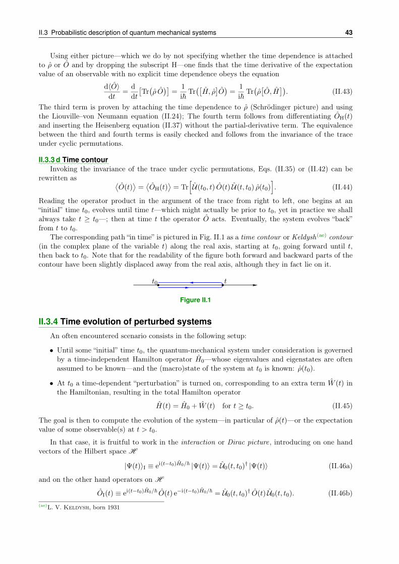
II.3 Probabilistic description of quantum mechanical systems 43
Using either picture—which we do by not specifying whether the time dependence is attachedto ρ or O and by dropping the subscript H—one finds that the time derivative of the expectationvalue of an observable with no explicit time dependence obeys the equation
d〈O〉dt
=d
dt
[Tr(ρ O)]
=1
i~Tr([H, ρ
]O)
=1
i~Tr(ρ[O, H
]). (II.43)
The third term is proven by attaching the time dependence to ρ (Schrödinger picture) and usingthe Liouville–von Neumann equation (II.24); The fourth term follows from differentiating OH(t)and inserting the Heisenberg equation (II.37) without the partial-derivative term. The equivalencebetween the third and fourth terms is easily checked and follows from the invariance of the traceunder cyclic permutations.
::::::II.3.3 d
:::::::::::::::Time contour
Invoking the invariance of the trace under cyclic permutations, Eqs. (II.35) or (II.42) can berewritten as ⟨
O(t)⟩
=⟨OH(t)
⟩= Tr
[U(t0, t) O(t) U(t, t0) ρ(t0)
]. (II.44)
Reading the operator product in the argument of the trace from right to left, one begins at an“initial” time t0, evolves until time t—which might actually be prior to t0, yet in practice we shallalways take t ≥ t0—; then at time t the operator O acts. Eventually, the system evolves “back”from t to t0.
The corresponding path “in time” is pictured in Fig. II.1 as a time contour or Keldysh(ae) contour(in the complex plane of the variable t) along the real axis, starting at t0, going forward until t,then back to t0. Note that for the readability of the figure both forward and backward parts of thecontour have been slightly displaced away from the real axis, although they in fact lie on it.
tt0
Figure II.1
II.3.4 Time evolution of perturbed systems
An often encountered scenario consists in the following setup:
• Until some “initial” time t0, the quantum-mechanical system under consideration is governedby a time-independent Hamilton operator H0—whose eigenvalues and eigenstates are oftenassumed to be known—and the (macro)state of the system at t0 is known: ρ(t0).
• At t0 a time-dependent “perturbation” is turned on, corresponding to an extra term W (t) inthe Hamiltonian, resulting in the total Hamilton operator
H(t) = H0 + W (t) for t ≥ t0. (II.45)
The goal is then to compute the evolution of the system—in particular of ρ(t)—or the expectationvalue of some observable(s) at t > t0.
In that case, it is fruitful to work in the interaction or Dirac picture, introducing on one handvectors of the Hilbert space H
|Ψ(t)〉I ≡ ei(t−t0)H0/~ |Ψ(t)〉 = U0(t, t0)† |Ψ(t)〉 (II.46a)
and on the other hand operators on H
OI(t) ≡ ei(t−t0)H0/~ O(t) e−i(t−t0)H0/~ = U0(t, t0)† O(t) U0(t, t0). (II.46b)(ae)L. V. Keldysh, born 1931
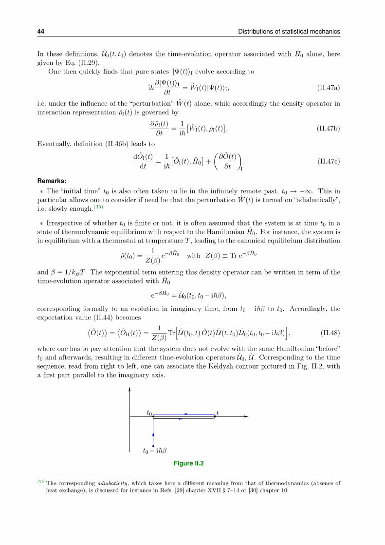
44 Distributions of statistical mechanics
In these definitions, U0(t, t0) denotes the time-evolution operator associated with H0 alone, heregiven by Eq. (II.29).
One then quickly finds that pure states |Ψ(t)〉I evolve according to
i~∂|Ψ(t)〉I∂t
= WI(t)|Ψ(t)〉I, (II.47a)
i.e. under the influence of the “perturbation” W (t) alone, while accordingly the density operator ininteraction representation ρI(t) is governed by
∂ρI(t)
∂t=
1
i~[WI(t), ρI(t)
]. (II.47b)
Eventually, definition (II.46b) leads to
dOI(t)
dt=
1
i~[OI(t), H0
]+
(∂O(t)
∂t
)I
. (II.47c)
Remarks:
∗ The “initial time” t0 is also often taken to lie in the infinitely remote past, t0 → −∞. This inparticular allows one to consider if need be that the perturbation W (t) is turned on “adiabatically”,i.e. slowly enough.(35)
∗ Irrespective of whether t0 is finite or not, it is often assumed that the system is at time t0 in astate of thermodynamic equilibrium with respect to the Hamiltonian H0. For instance, the system isin equilibrium with a thermostat at temperature T , leading to the canonical equilibrium distribution
ρ(t0) =1
Z(β)e−βH0 with Z(β) ≡ Tr e−βH0
and β ≡ 1/kBT . The exponential term entering this density operator can be written in term of thetime-evolution operator associated with H0
e−βH0 = U0(t0, t0− i~β),
corresponding formally to an evolution in imaginary time, from t0− i~β to t0. Accordingly, theexpectation value (II.44) becomes⟨
O(t)⟩
=⟨OH(t)
⟩=
1
Z(β)Tr[U(t0, t) O(t) U(t, t0) U0(t0, t0− i~β)
], (II.48)
where one has to pay attention that the system does not evolve with the same Hamiltonian “before”t0 and afterwards, resulting in different time-evolution operators U0, U . Corresponding to the timesequence, read from right to left, one can associate the Keldysh contour pictured in Fig. II.2, witha first part parallel to the imaginary axis.
tt0
t0− i~β
Figure II.2
(35)The corresponding adiabaticity , which takes here a different meaning from that of thermodynamics (absence ofheat exchange), is discussed for instance in Refs. [29] chapter XVII § 7–14 or [30] chapter 10.
II.4 Statistiscal entropy 45
II.4 Statistiscal entropyThe probabilistic approach advocated in Sec. II.1 arises from a lack of knowledge on the microscopicstate of the system. This raises the question of how much information is missing, if only discreteprobabilities pk or a probability density ρN are known.
Intuitively, the missing information is “small” when the probability distribution takes significantvalues for only a few microstates, while it is larger in case the distribution extends over manystates. To make sense of this intuition, a measure of (missing) information in probability theory,the statistical entropy, is introduced in Sec. II.4.1. This measure is then applied to the probabilitydistributions that describe quantum-mechanical (Sec. II.4.2) or classical (Sec. II.4.3) systems.
II.4.1 Statistical entropy in information theory
For the sake of brevity, we shall in the following consider only discrete probability distributions,with the exception of definition (II.50). The generalization to the case of continuous distributionsis straightforward.
Consider M events ω1, . . . , ωM with respective probabilities p1, . . . , pM . In order to quantifythe “uncertainty” (or “missing information”, “ignorance”) corresponding to the use of this probabilitydistribution, C. Shannon(af) [31] has introduced the statistical entropy
Sstat(p1, . . . , pM ) ≡ −kM∑m=1
pm ln pm, (II.49)
with k an arbitrary positive constant. Sstat(p1, . . . , pM ) is thus exactly equal to the average valueof −k ln pm.
In information theory one usually takes k = 1/ ln 2, so that
Sstat(p1, . . . , pM ) =
⟨log2
1
pm
⟩,
and the statistical entropy is dimensionless.(36)
The quantity − log2 pm is the information content or self-information associated with the eventωm (for Shannon, the events were possible meaningful messages in a given language). Thus, theoccurrence of a message ωm with low probability is more informative, more surprising than thatof a more probable message.
In the case of a continuous probability distribution, described by a probability density p(x), thestatistical entropy is given by
Sstat
(p(x)
)≡ −k
∫p(x) ln p(x) dx. (II.50)
Sstat is here also equal to the expectation value of the logarithm of the distribution.
II.4.2 Statistical entropy of a quantum-mechanical system
The notion of statistical entropy can now be applied to the probability distributions introducedin the description of macroscopic quantum-mechanical systems.(36)In this context, the unit of the statistical entropy is the bit.(af)C. Shannon, 1916–2001

46 Distributions of statistical mechanics
Let ρ denote the density operator associated with a quantum-mechanical mixture of states, witheigenvalues p1, . . . , pM . The corresponding statistical entropy is defined as
S(ρ)≡ −kB
∑m
pm ln pm = −kB Tr(ρ ln ρ
), (II.51)
where the second identity follows at once in a basis in which ρ is diagonal. Here kB is the Boltz-mann(ag) constant, kB = 1.38× 10⁻²³ J.K−1.
Remark: The first identity matches the definition of the entropy by Gibbs (1878), the secondcorresponds to the von Neumann entropy (1927).
II.4.3 Statistical entropy of a classical system
The missing information associated with the use of a probability density on phase space, as isthe case for macroscropic classical systems, can similarly be quantified with the statistical entropy.For a classical system with fluctuating particle number N , the statistical entropy reads
S(ρ) = −kB∑N
∫ρN (qi, pi) ln ρN (qi, pi) d6NV . (II.52)
This statistical entropy globally enjoys the same properties as its quantum-mechanical counter-part (II.51), up to an important exception. Since a probability density is not bounded from aboveto 1, S(ρ) can be negative, and actually has no minimum. One can find phase-space densities suchthat S(ρ) is as negative as one wants, i.e. S(ρ) can go to −∞. Such densities actually require asimultaneous knowledge of both positions and momenta of particles, which violate the Heisenberguncertainty relations of quantum mechanics.
Bibliography for Chapter II• Kubo et al., Statistical physics I: Equilibrium statistical physics [32], chapter 1.3.
• Landau & Lifshitz, Course of theoretical physics Vol. 1: Mechanics [26], chapter VII § 46 andVol. 5: Statistical physics, part 1 [3], chapter I.
• Le Bellac, Mortessagne & Batrouni, Equilibrium and non-equilibrium statistical thermodynam-ics [9], chapter 2.1–2.2.
• Pottier, Nonequilibrium statistical physics [6], chapter 3.
• Zwanzig, Nonequilibrium statistical mechanics [7], chapters 2.1 & 6.1.
(ag)L. Boltzmann, 1844–1906
CHAPTER III
Reduced classical phase-spacedensities and their evolution
The description of a classicalN -body systems relies on theN -particle phase space Γ: the evolution ofthe system is represented by a trajectory (qi(t), pi(t)) solution of the Hamilton equations (II.1)—corresponding to the sequence of microstates occupied by the system at successive instants—, whileobservables are functions ON
(qi, pi
)on Γ. If, as is generally the case for macroscopic sys-
tems, the system state is only known on a statistical basis, one also needs the probability densityρN(t, qi, pi
)on Γ, whose time evolution is governed by the Liouville equation (II.10b), see
Sec. II.2.In the large majority of cases, the macroscopic quantities of interest are a measure for the
expectation value of microscopic observables that only involve few particles, often only one or two.For instance, the temperature is related to the average kinetic energy of the particles in the system,which involves a single-particle observable. To compute the expectation values of such observables,it is worthwhile to introduce reduced phase-space densities, which integrate out the irrelevant degreesof freedom (Sec. III.1). From the Liouville equation for the Γ-space probability density ρN , one canthen derive the equations of motion governing the dynamics of the reduced densities (Sec. III.2).
In this chapter and the following one, the positions and momenta of the N particles will bedenoted by ~ri and ~pi respectively, where i = 1, . . . , N labels the particle. Accordingly, the argumentof a function on the Γ-space of the N particles will be written ~ri, ~pi or ~r1,~p1, . . . ,~rN ,~pN insteadof qj, pj.
III.1 Reduced phase-space densitiesConsider a system of N particles, which for simplicity are first assumed to be identical. Startingfrom the N -particle density ρN (t,~r1,~p1, . . . ,~rN ,~pN ) and integrating out the space and momentumcoordinates of N − 1 particles, one defines the single-particle phase-space density
f1(t,~r,~p) ≡ αN,1∫ρN (t,~r,~p,~r2,~p2, . . . ,~rN ,~pN ) d6(N−1)V (III.1a)
where d6(N−1)V is the infinitesimal volume element in the subspace spanned by the variables~r2,~p2, . . . ,~rN ,~pN . The remaining single-particle phase space is often referred to as µ-space, soas to distinguish it from the Γ-space.
Similarly, one introduces the two-particle phase-space density
f2(t,~r,~p,~r ′,~p ′) ≡ αN,2∫ρN (t,~r,~p,~r ′,~p ′,~r3,~p3, . . . ,~rN ,~pN ) d6(N−2)V . (III.1b)
More generally, integrating out the positions and momenta of N − k particles in the Γ-spacedensity ρN leads to a k-particle phase-space density fk.
Remark: For a system of identical—i.e. quantum-mechanically indistinguishable—particles, thedensity ρN should be symmetric under the exchange of any two particles, i.e. of the variables ~ri, ~pi

48 Reduced classical phase-space densities and their evolution
and ~rj , ~pj for any i, j. Accordingly, which N − k positions and momenta are being integrated outin the definition of the reduced k-particle density fk is actually unimportant, and any choice leadsto the same reduced density.
The definitions (III.1a) and (III.1b) involve constants αN,1, αN,2. These are often chosen so thatthe single- and two-particle phase-space densities are respectively normalized to∫
f1(t,~r,~p) d3~r d3~p = N, (III.2a)
i.e. the total number of particles, and∫f2(t,~r,~p,~r ′,~p ′) d3~r d3~p d3~r ′ d3~p ′ = N(N − 1), (III.2b)
that is, the total number of ordered pairs. More generally, one requires that the integral of fk bethe total number of ordered k-tuples. This requirement dictates for identical particles the choiceαN,k = 1/(2π~)3k, independent of N . With these normalizations, f1(t,~r,~p) d3~r d3~p is the averagenumber of particles in the infinitesimal volume element d3~r d3~p around the µ-space point (~r,~p)at time t, while f2(t,~r,~p,~r ′,~p ′) d3~r d3~p d3~r ′ d3~p ′ is the average number of ordered pairs with oneparticle in the volume element d3~r d3~p around (~r,~p) and the other in d3~r ′ d3~p ′ around (~r ′,~p ′).The various fk are thus number densities in the respective phase spaces, rather than probabilitydensities.
Integrating the single-particle phase-space density (III.1a) normalized according to Eq. (III.2a)over momentum, one recovers the usual particle number density (in position space)
n(t,~r) ≡∫f1(t,~r,~p) d3~p. (III.3a)
Remarks:∗ Up to the normalization [N !/(N − k)! instead of 1], the reduced phase-space densities fk aremarginal distributions (see Appendix B.4.1) of the Γ-space density ρN .
∗ Given the normalization adopted here, the densities fk are dimensionful quantities. It is some-times preferable to work with dimensionless densities, namely fk ≡ (2π~)3kfk, which correspond tothe simpler normalization constant αN,k = 1 for all k. Integrating f1 over a spatial volume on whichthe system is homogeneous then yields the so-called phase-space occupancy—where “phase space”actually means momentum space.
The various results of this chapter, as e.g. the BBGKY hierarchy (III.14), still hold when replacingthe reduced densities fk by the dimensionless fk, provided every momentum-space volume elementd3~p appearing in an integral is replaced by d3~p/(2π~)3. For instance,
n(t,~r) ≡∫
f1(t,~r,~p)d3~p
(2π~)3. (III.3b)
∗ The reduced densities fk depend on the underlying statistical ensemble. Here, since the numberof particles N is fixed, we are implicitly considering the canonical ensemble, yet this is just for thesake of simplicity.
In the “grand-canonical” case of a fluctuating particle number, integrating the phase-space densityρ defined in § II.2.5 over the irrelevant degrees of freedom yields the reduced k-particle density
fk =
∞∑N=k
πNfk|N−k
where fk|N−k is the (“canonical”) reduced k-particle distribution under the condition that thereare exactly N particles in the system while πN is the probability that this is the case. Accordingly,f1 is then normalized to 〈N〉, f2 to 〈N(N − 1)〉, and so on.The reader can check that for a classical ideal gas, f2(t,~r,~p,~r ′,~p ′) = f1(t,~r,~p)f1(t,~r ′,~p ′) in thegrand-canonical case—which can be interpreted as signaling the absence of correlations betweenparticles—, while the identity does not hold when the total particle number is fixed.
III.2 Time evolution of the reduced phase-space densities 49
With the help of the µ-space density f1, the expectation value of a single-particle observableO1(~r,~p) reads
⟨O1(t)
⟩t
=
∫O1(~r,~p) f1(t,~r,~p) d3~r d3~p∫
f1(t,~r,~p) d3~r d3~p
. (III.4)
The expectation value of a two-particle observable can similarly be expressed as an average weightedby the two-particle density f2.
III.2 Time evolution of the reduced phase-space densitiesWe now deduce from the Liouville equation (III.5) the equations of motion for the reduced phase-space densities, first for a system of particles in the absence of vector potential (Sec. III.2.2), thenfor charged particles in a external vector potential (Sec. III.2.3).
III.2.1 Description of the system
Consider identical pointlike particles of mass m, without internal degrees of freedom, whosepositions and canonical momenta will be denoted by ~ri and ~pi. For a system of N such particles,the Liouville equation (II.10b) can be recast as
∂ρN(t, ~rj, ~pj
)∂t
+N∑i=1
~ri · ~∇~riρN(t, ~rj, ~pj
)+
N∑i=1
~pi · ~∇~piρN(t, ~rj, ~pj
)= 0, (III.5a)
where ~∇~ri , ~∇~pi stand for the three-dimensional gradients whose coordinates are the derivatives withrespect to the canonical variables ~ri, ~pi. In turn, ~ri—i.e. the velocity ~vi of particle i—and ~pi denotethe time derivatives of the canonical variables. Invoking the Hamilton equations (II.1) and droppingthe variables, the Liouville equation becomes
∂ρN∂t
+N∑i=1
~∇~piHN · ~∇~riρN −N∑i=1
~∇~riHN · ~∇~piρN = 0 (III.5b)
with HN the Hamilton function of the system, which we shall specify later in this section.
In both this chapter and the following we shall implicitly work in the “thermodynamic limit”of an infinitely many of particles occupying an infinitely large volume, thereby allowing for aninfinitely large total energy of the system. As a result, both the Cartesian components of spatialand momentum variables can take values spanning the whole real axis from −∞ to +∞. Now, toensure its normalizability [Eq. (II.3)], the probability density ρN must vanish when one of its phase-space variables goes to infinity: the partial differential equation (III.5a) is thus to be complementedwith the boundary conditions
lim|~ri|→∞
ρN(t, ~rj, ~pj
)= 0 and lim
|~pi|→∞ρN(t, ~rj, ~pj
)= 0 ∀i ∈ 1, . . . , N. (III.6)
Accordingly, integrals of the type∫~∇~riρN
(t, ~rj, ~pj
)d3~ri resp.
∫~∇~piρN
(t, ~rj, ~pj
)d3~pi (III.7)
over the whole allowed range for ~ri resp. ~pi identically vanish.
For the sake of completeness, let us briefly mention some of the necessary changes taking place ifthe spatial volume V occupied by the system is not infinite—as is e.g. the case of a gas enclosedin a fixed box. In short, the treatment becomes slightly more tedious.

50 Reduced classical phase-space densities and their evolution
First, the total number N of particles is then finite, and so is the total energy of the system. Asa result, the (kinetic) energy of an individual particle cannot be infinitely large, which meansthat the range of allowed momentum values is finite: the behavior of ρN at the edges of themomentum range is no longer obvious, although it is natural to assume that ρN vanishes.
Since the spatial volume is finite, the variables ~ri are also restricted to a finite range. It isthen necessary to specify the boundary conditions at these spatial edges (“walls”). A usefulchoice is to assume that the boundaries behave like perfect mirrors for the particles, which arethus reflected elastically according to the Snell(ah)–Descartes(ai) law of reflection: this has theadvantage of ensuring the conservation of kinetic energy; however such a particle-wall collisiondoes not conserve (linear) momentum, which is unsatisfactory. The “good” approach is then toresort to a microscopic description of the walls themselves, which become part of the systemunder study.
Let us now specify the Hamilton function HN of the system. For the sake of simplicity, we shallassume that the particles can only interact with each other pairwise, i.e. we discard possible genuinethree-, four-, . . . , many-body interaction terms. These two-body interactions can be described interms of an interaction potential W ,(37) which will be assumed to depend on the inter-particledistance only.
We also allow for the possible presence of external potentials acting on the particles. Here onehas to distinguish between two possibilities. Thus, a scalar potential V (t,~r)—e.g. electrostatic,(Newtonian) gravitational, or a potential well enclosing particles in a specified volume—only con-stitutes a minor modification, since it does not affect the canonical momentum ~pi conjugate toposition. In contrast, any vector potential ~A(t,~r) directly enters the canonical momentum, so thatwe shall have to discuss the gauge invariance of the evolution equations for the reduced phase-spacedensities.
In the absence of vector potential, the Hamilton function of the system is of the type
HN =
N∑i=1
~p 2i
2m+
N∑i=1
V (t,~ri) +∑
1≤i<j≤NW(∣∣~ri −~rj∣∣). (III.8)
For a system of electrically charged particles with charge q in an external electromagnetic fielddescribed by scalar and vector potentials (φ, ~A), the Hamiltonian reads
HN =N∑i=1
[~pi − q ~A(t,~ri)
]22m
+N∑i=1
qφ(t,~ri) +∑
1≤i<j≤NW(∣∣~ri −~rj∣∣), (III.9)
where the energy corresponding to the scalar potential has been denoted by qφ instead of V .
In the remainder of this Chapter, we shall use the shorthand notations Wij ≡ W(∣∣~ri −~rj∣∣) as
well as~Fi ≡ −~∇~riV (~ri), (III.10a)
~Kij ≡ −~∇~riW(∣∣~ri −~rj∣∣), (III.10b)
for the forces upon particle i due to the external potential V and to particle j 6= i, respectively. Inaccordance with Newton’s third law,
~Kij = − ~Kji, (III.10c)
which follows from ~∇~rjWij = −~∇~riWij and the relabeling of particles.
Remarks:∗ The above forms of the Hamilton function implicitly assume that the forces at play in the systemare additive, as is always the case in Newtonian physics.(37)More precisely, W
(∣∣~ri −~rj∣∣) is the interaction potential energy.
(ah)W. Snellius, 1580–1626 (ai)R. Descartes, 1596–1650

III.2 Time evolution of the reduced phase-space densities 51
∗ In the absence of interactions, the Hamilton function (III.8) clearly reduces to that of a classicalideal gas.
III.2.2 System of neutral particles
In the absence of external vector potential, the Hamilton equations (II.1) with the Hamiltonfunction (III.8) read
~ri = ~∇~piHN =~pim, ~pi = −~∇~riHN = ~Fi +
∑j 6=i
~Kij . (III.11)
The first equation simply states that linear momentum and canonical momentum coincide, fromwhere it follows that the second equation is Newton’s second law.
Accordingly, the Liouville equation (III.5) becomes
∂ρN∂t
+N∑i=1
~vi · ~∇~riρN +N∑i=1
~Fi · ~∇~piρN +N∑i=1
N∑j=1j 6=i
~Kij · ~∇~piρN = 0. (III.12)
:::::::III.2.2 a
:::::::::::::::::::BBGKY hierarchy
The reduced k-particle phase density fk(t,~r1,~p1, . . . ,~rk,~pk) follows from the Γ-space probabilitydensity ρN after integrating out the degrees of freedom of the remaining N − k particles. Similarly,integrating the Liouville equation (III.12) over the positions and momenta ~rj , ~pj of N − k particlesgives the evolution equation obeyed by fk.
This integration is made simpler by the boundary conditions (III.6): since the velocity ~vi resp.the force ~Fi is independent of ~ri resp. ~pi, it can be factored outside of the integral∫
~vi · ~∇~riρN d3~ri resp.∫~Fi · ~∇~piρN d3~pi, (III.13)
leaving an integral of the type (III.7), which identically vanishes.Additionally, we shall assume that we are allowed to exchange the integration and partial differen-tiation operations when needed.
Integrating the Liouville equation (III.12) over the N − 1 particles labeled 2, 3, . . . , N withthe proper normalization factor αN,1 = 1/(2π~)3 yields for the evolution of the single-particledensity (III.1a) the equation
∂f1(t,~r1,~p1)
∂t+ ~v1 · ~∇~r1f1(t,~r1,~p1) + ~F1 · ~∇~p1f1(t,~r1,~p1)
+
N∑j=2
1
(2π~)3
∫~K1j · ~∇~p1ρN
(t, ~ri, ~pi
)d6(N−1)V (2, . . . , N) = 0,
where the notation d6(N−1)V (2, . . . , N) emphasizes the labels of the particles which are integratedout. In the integral in the second line, it is convenient to write
d6(N−1)V (2, . . . , N) =1
N − 1
d3~rj d3 ~pj(2π~)3
d6(N−2)V (2, . . . , j−1, j+1, . . . , N)
to isolate particle j from the N −2 particles i 6= j. The latter are then straightforwardly dealt with:integrating over their phase-space coordinates yields, together with the factor 1/(2π~)6 = αN,2,precisely the two-particle phase-space density f2(t,~r1,~p1,~rj ,~pj), i.e.
1
(2π~)3
∫~K1j ·~∇~p1ρN
(t, ~ri, ~pi
)d6(N−1)V (2, . . . , N) =
1
N−1
∫~K1j ·~∇~p1f2(t,~r1,~p1,~rj ,~pj) d3~rj d3~pj .
Thanks to the indistinguishability of the particles, the remaining integral over d3~rj d3~pj is actuallyindependent of the value of the index j: the sum over j gives N − 1 times the same contribution,

52 Reduced classical phase-space densities and their evolution
which may be rewritten with the dummy integration variables ~r2,~p2, while the factor N − 1 cancelsthat present in the denominator of d6(N−1)V . All in all, one thus obtains(
∂
∂t+ ~v1 · ~∇~r1 + ~F1 · ~∇~p1
)f1(t,~r1,~p1) = −
∫~K12 · ~∇~p1f2(t,~r1,~p1,~r2,~p2) d3~r2 d3~p2. (III.14a)
That is, the equation governing the evolution of the single-particle density f1 involves the two-particle density f2.
By integrating out N−2 particles in the Liouville equation (III.12), one finds in a similar mannerthe evolution equation for the dynamics of the reduced two-particle density(38)
[∂
∂t+ ~v1 ·~∇~r1 + ~v2 ·~∇~r2 + ~F1 ·~∇~p1 + ~F2 ·~∇~p2 + ~K12 ·
(~∇~p1−~∇~p2
)]f2(t,~r1,~p1,~r2,~p2) =
−∫ (
~K13 ·~∇~p1 + ~K23 ·~∇~p2)f3(t,~r1,~p1,~r2,~p2,~r3,~p3) d3~r3 d3~p3.
(III.14b)
In turn, the evolution equation for f2 involves the three-particle phase-space density f3.
The only trick in deriving this form of the evolution equation consists in using relation (III.10c)to rewrite ~K21 · ~∇~p2 as − ~K12 · ~∇~p2 .
This generalizes to the equation of motion for the reduced k-particle density fk—obtained byintegrating out N−k particles in the Liouville equation (III.12)—, which is not closed, but dependson the (k+1)-particle density fk+1 for 1 ≤ k < N :[
∂
∂t+
k∑j=1
(~vk ·~∇~rj + ~Fj ·~∇~pj
)+∑
1≤i<j≤k
~Kij ·(~∇~pi−~∇~pj
)]fk(t,~r1,~p1, . . . ,~rk,~pk) =
−∫ k∑
j=1
~Kj,k+1 ·~∇~pjfk+1(t,~r1,~p1, . . . ,~rk,~pk,~rk+1,~pk+1) d3~rk+1 d3~pk+1.
(III.14c)
The meaning of this equation is rather clear: The left-hand side describes the “free”, or stream-ing evolution of fk, involving only the k particles under consideration—including their reciprocalinteractions. On the other hand, the right-hand side is a collision term describing the interactionbetween any of these k particles and a partner among the group of the other, not measured particles.
Eventually, the N -particle phase-space density fN is simply ρN multiplied by a normalizationfactor, so that the evolution equation for fN is closed, since it is the Liouville equation (III.12) itself[
∂
∂t+
N∑j=1
(~vj · ~∇~rj + ~Fj · ~∇~pj
)+
∑1≤i<j≤N
~Kij ·(~∇~pi− ~∇~pj
)]fN (t,~r1,~p1, . . . ,~rN ,~pN ) = 0. (III.14d)
Together, the coupled equations (III.14a)–(III.14d) constitute the so-called BBGKY hierarchy ,where the initials stand for Bogolioubov(aj)–Born(ak)–Green(al)–Kirkwood(am)–Yvon(an) (in alpha-betical and reverse chronological order).
The system of equations (III.14) is exact, in the sense that it is strictly equivalent to the Liouvilleequation for the probability density in Γ-space. Yet since the hierarchy involves all reduced densities,and accordingly N equations, one loses the simplification aimed at when considering single-or two-particle densities only. To recover some simplicity—and thereby be able to actually compute theevolution of the system—, one has to choose a closure procedure, based on physical arguments,(38)Note that there is an erroneous factor of 1
2in Eq. (3.60) of Ref. [33].
(aj)N. N. Bogolioubov, 1909–1992 (ak)M. Born, 1882–1970 (al)H. S. Green, 1920–1999 (am)J. G. Kirkwood,1907–1959 (an)J. Yvon, 1903–1979

III.2 Time evolution of the reduced phase-space densities 53
which amounts to truncating the hierarchy at some level. This is most often done after Eq. (III.14a),sometimes after Eq. (III.14b).
The most drastic closure prescription, which is discussed in § III.2.2 b below, consists in fullyneglecting interactions. A similar, yet physically richer, scheme is to keep Eq. (III.14a) intact, yet toassume that the right-hand side of Eq. (III.14b) vanishes. Alternative procedures will be consideredin § III.2.3 b and in the next chapter.
Remarks:
∗ If the number of particles in the system is not fixed, i.e. in a grand-canonical description, thereis no upper bound to the hierarchy.
∗ The generalization to a system consisting of several particle types, labeled a, b. . . , interactingwith each other over respective potentialsW ab, is quite straightforward. One first needs to introducethe reduced densities f bk, f
bk. . . , for having k particles of a given type in an infinitesimal k-particle
phase-space volume, as well as “mixed” densities fab...kakb...for having ka particles of type a, kb particles
of type b. . . within corresponding phase-space volume elements. These various densities—includingthe mixed ones—then obey coupled equations similar to those of the hierarchy (III.14), with inaddition sums over the various particle types. For instance, the evolution equation for fa1 involveson its right-hand side not only fa2 , but also all fab1,1 involving the particles of type b 6= a which coupleto those of type a.
:::::::III.2.2 b
::::::::::::::::::::::::::::::::::::::::::::::::::::::::::::::::::::::::::::::::System of non-interacting neutral particles: single-particle Liouville equation
Consider first the case where the particles in the system are not interacting, i.e. whenW vanishesidentically. The Hamilton function HN can then be expressed as the sum over the N particles of asingle-particle Hamiltonian h ≡ ~p 2/2m+ V (t,~r).
Under these conditions, the various equations of the BBGKY hierarchy (III.14) decouple fromeach other. For instance, the evolution equation (III.14a) for the dynamics of the single-particledensity f1 becomes the single-particle Liouville equation (or collisionless Boltzmann equation)
∂f1(t,~r,~p)
∂t+ ~v · ~∇~rf1(t,~r,~p) + ~F (t,~r) · ~∇~pf1(t,~r,~p) = 0, (III.15)
with ~F = −~∇~rV the external force acting on particles. The contribution(~v ·~∇~r+ ~F ·~∇~p
)f1—which is
actually the Poisson bracket in µ-space of f1(t,~r,~p) and the single-particle Hamiltonian h(~r,~p)—isoften referred to as drift term.
The latter implicitly defines two time scales of the system, namely
τs ∼(~v · ~∇~r
)−1, τe ∼
(~F · ~∇~p
)−1. (III.16)
τs is the time for a particle to cross the typical distance over which the single-particle density f1 isvarying. As such, it is also the characteristic time scale for smoothing out spatial inhomogeneitiesof the single-particle distribution.
In turn, τe is the typical time associated with the gradient imposed by the external potential V .It is thus also the characteristic time scale over which the system inhomogeneities will relax underthe influence of ~F to the equilibrium solution matching the external potential. τe is generally largerthan τs.
Remark: One sees at once that the other equations of the hierarchy involve the same two timescales, and no further one. That is, any fk evolves with the same time scale as f1, which will nolonger be the case in the presence of interactions.
:::::::III.2.2 c
:::::::::::::::::::::::::::::::::::::::Influence of inter-particle interactions
Let us now take into account the effect of interactions between particles, considering the firstequation (III.14a) of the BBGKY hierarchy with a non-vanishing right-hand side. On the other

54 Reduced classical phase-space densities and their evolution
hand, we assume that the right member of the second equation (III.14b) vanishes, i.e. we neglectthe influence of the three-particle density on the evolution of f2.
Inspecting the resulting evolution equations, one finds that there is a new time scale besides τs
and τe, set by the intensity of the pairwise interaction, namely
τc ∼(~K · ~∇~p
)−1. (III.17)
From the evolution equation for the two-particle density f2, the collision duration τc appears as thecharacteristic time scale over which collisions between two particles smooth out the differences intheir respective momentum distributions. τc is actually the smallest time scale, much smaller thanτs and τe.
As a result, the evolution of f2 is actually quicker than that of f1 in the non-interacting case,for this quick time scale is absent from the single-particle Liouville equation (III.15). In turn, itmeans that when particles are allowed to interact with each other, the pace for the evolution of f1
is not set by its slow drift term, but by the fast collision term in the right-hand side.
Remark: One could then wonder whether the time scale for the evolution of f2 is not governed bythe collision term involving f3, which we are neglecting here. It can be checked that this is not thecase in the dilute regime in which only pairwise interactions are important.
In the derivation of the BBGKY hierarchy (III.14), we have from the start assumed that particlesonly interact with each other in pairs. It is quite straightforward to see what would happen if wealso allowed for genuine interactions between three, four or more particles at once.
The effect of the latter is simply to add further contributions to the collision and drift terms ofthe equations of motion. For instance, when allowing for three-particle interactions, the equationgoverning the evolution of fk would not only involve fk+1, but also fk+2, corresponding to the casewhere one particle among the k under consideration is interacting with two “outsiders”. Despite thiscomplication, one can still derive an exact hierarchy of equations.
:::::::III.2.2 d
::::::::::::::::::::::::::::::::::::::::::::::BBGKY hierarchy in position-velocity space
Instead of characterizing a pointlike particle by a point in its µ-space, i.e. by its position andcanonical momentum, one sometimes rather makes use of a point in position-velocity space, i.e. onespecifies the positions and velocities of the particles.
In that representation, one can similarly introduce k-particle densities over a k-particle position-velocity space, hereafter denoted as f~v,k, such that f~v,k(t,~r1, ~v1, . . . ,~rk, ~vk) d3~r1 d3~v1 · · · d3~rk d3~vk isthe number of particles in the infinitesimal volume element d3~r1 d3~v1 · · · d3~rk d3~vk around the point(~r1, ~v1, . . . ,~rk, ~vk). The density f~v,k is related to the reduced phase-space density fk by the relation
f~v,k(t,~r1, ~v1, . . . ,~rk, ~vk) d3~r1 d3~v1 · · · d3~rk d3~vk = fk(t,~r1,~p1, . . . ,~rk,~pk) d3~r1 d3~p1 · · · d3~rk d3~pk.
(III.18)
In the case considered in this section of a system of particles in absence of an external vectorpotential, the velocity ~v of a particle is simply proportional to its canonical momentum ~p, so thatf~v,k is trivially proportional to fk and ~∇~v to ~∇~p. One checks at once that the position-velocity spacedensities obey a similar BBGKY hierarchy as the phase-space densities, the only modification beingthe substitutions of ~∇~pj by by ~∇~vj and ~pj by ~vj . For instance, the first equation of the hierarchyreads(
∂
∂t+ ~v1 · ~∇~r1 +
~F1
m· ~∇~v1
)f~v,1(t,~r1, ~v1) = −
∫ ~K12
m· ~∇~v1f~v,2(t,~r1, ~v1,~r2, ~v2) d3~r2 d3~v2. (III.19)
The real advantage of the formulation in position-velocity space is for the case, addressed innext section, of a system of charged particles in the presence of an external vector potential.

III.2 Time evolution of the reduced phase-space densities 55
III.2.3 System of charged particles
We now briefly introduce the subtleties which appear when the particles in the system arecoupled to an external vector potential, as is for instance the case of electrically charged particlesin an external (electro)magnetic field.
In this subsection, we shall exceptionally denote the canonical momentum conjugate to position~ri as ~πi, and the reduced phase-space densities as f~π,k.
:::::::III.2.3 a
::::::::::::::::::::::::::::::::::::::::::::::::::::::Phase-space vs. position-velocity space description
The evolution equations of the BBGKY hierarchy (III.14) have been derived starting from theLiouville equation on phase space, i.e. within the framework of a Hamiltonian formalism. A similarapproach can also be adopted in the presence of an external vector field, yet there appear twocomplications, which can be traced back to the expression of the canonical momentum, derivedfrom the Hamilton equations following from the Hamilton function (III.9)
~ri =~πi − q ~A(t, ~ri)
m, (III.20a)
~πi = −q~∇~r φ(t,~ri) + q(~ri · ~∇~r
)~A(t, ~ri) + q~ri ×
[~∇~r × ~A(t, ~ri)
]+∑j 6=i
~Kij , (III.20b)
where in the second equation we have made use of the first one.
• The time derivatives ~vi = ~ri and ~πi are no longer independent of ~ri or ~πi, respectively. Asa consequence, the integrals (III.13)—in which ~∇~pi is to be replaced by ~∇~πi—are no longertrivial. Yet by using the Hamilton equations, one can show at the cost of a few integrationby parts that the contributions of these integrals vanish, so that the evolution of the reducedphase-space density f~π,k is eventually governed by an equation with the same structure asEq. (III.14c), although with different factors in front of the gradients.
For example, the collisionless evolution equation for the single-particle density f~π,1 is∂f~π,1(t,~r, ~π)
∂t+ ~v · ~∇~rf~π,1(t,~r, ~π) + ~π · ~∇~πf~π,1(t,~r, ~π) = 0, (III.21)
which differs from Eq. (III.15) because of the Hamilton equations (III.20).
• The second issue with the evolution equations for the reduced phase-space densities derivedwithin the Hamiltonian formalism is that they are not manifestly gauge invariant, which isquite natural since the canonical momenta ~πi themselves are gauge-dependent, see Eq. (III.20).
To remedy the latter problem, it is convenient to consider the densities in position-velocity space,instead of phase space. The resulting equations—which take the same form as in the absence ofvector potential—only involve gauge invariant quantities. For instance, the collisionless evolutionequation for the single-particle density f~v,1 is
∂f~v,1(t,~r,~v)
∂t+ ~v · ~∇~rf~v,1(t,~r,~v) +
~FL
m· ~∇~vf~v,1(t,~r,~v) = 0, (III.22)
with ~FL = q( ~Eext +~v× ~Bext) the Lorentz(ao) force due to external electromagnetic fields ( ~Eext, ~Bext).This equation is exactly the same as Eq. (III.19) in the absence of collision term. One can checkthat Eqs. (III.21) under consideration of Eq. (III.20) and Eq. (III.22) are actually equivalent.
Alternatively, one most often works in the space spanned by the positions ~ri and the linearmomenta ~pi = m~vi. The densities fk on that space obey exactly the same equations (III.14) asin the case of neutral particles. This is obvious in case there is no vector potential—conjugateand linear momenta ~πi and ~pi then coincide—and justifies our retaining the same notation as inSec. III.2.2 for the densities.(ao)H. A. Lorentz, 1853–1926
56 Reduced classical phase-space densities and their evolution
:::::::III.2.3 b
:::::::::::::::::Vlasov equation
An important example of macroscopic system of electrically charged particles is that of aplasma—where one actually has to consider two different types of particles, with positive andnegative charges respectively, to ensure the mechanical stability.
In that context, Vlasov(ap) has introduced a closure prescription for the corresponding BBGKYhierarchy, which consists in assuming that the two-particle density factorizes into the product ofsingle particle densities(39)
f2(t,~r1,~p1,~r2,~p2) ' f1(t,~r1,~p1) f1(t,~r2,~p2). (III.23)
Under this assumption, Eq. (III.19) becomes closed and can be rewritten as[∂
∂t+ ~v1 · ~∇~r1 +
(~F1 +
∫~K12f1(t,~r2,~p2) d3~r2 d3~p2
)· ~∇~p1
]f1(t,~r1,~p1) = 0, (III.24)
with ~F1 = q(~Eext + ~v × ~Bext
)the Lorentz force due to the external electromagnetic field. This
constitutes the Vlasov equation.The integral term inside the brackets can be viewed as an average force exerted by the partner
particle 2 on particle 1. In the specific case of an electromagnetic plasma—assuming for simplicitythat the particles in the system have velocities much smaller than the speed of light, so that theirmutual interaction is mostly of Coulombic(aq) nature—this average force is that due to the meanelectrostatic field created by the other particles:[
∂
∂t+ ~v1 · ~∇~r1 + q
(~E ′ + ~Eext + ~v × ~Bext
)· ~∇~p1
]f1(t,~r1,~p1) = 0
with~E ′ ≡ 1
q
∫~K12f1(t,~r2,~p2) d3~r2 d3~p2.
The Vlasov assumption is thus an instance of mean-field approximation.
Remark: The Vlasov equation (III.24) is nonlinear, and thus non-trivial. In practice it must besolved in a self-consistent way, since the mean field in which f1 evolves depends on f1 itself.
Bibliography for Chapter III• Huang, Statistical Mechanics [33], chapter 3.5.
• Landau & Lifshitz, Course of theoretical physics. Vol. 10: Physical kinetics [5], chapter I § 16.
• Pottier, Nonequilibrium statistical physics [6], chapter 4.
(39)We do not write this hypothesis as an identity with an = sign to accommodate the possible mismatch betweenthe normalizations of f1 and f2.
(ap)A. A. Vlasov, 1908–1975 (aq)C. A. Coulomb, 1736–1806
CHAPTER IV
Boltzmann equation
In the previous chapter, it has been shown that the Liouville equation describing the evolution inΓ-space of the probability density for a collection of many classical particles can be equivalentlyrecast as a system of coupled evolution equations, the BBGKY hierarchy, for the successive reducedphase-space densities fk. To become tractable, the hierarchy has to be truncated, by closing thesystem of equations on the basis of some physical ansatz.
A non-trivial example of such a prescription is the so-called assumption of molecular chaos,introduced by L. Boltzmann. This hypothesis provides a satisfactory recipe for systems of weaklyinteracting particles, the paradigmatic example thereof being a dilute gas. In such systems, thetime scales characterizing the typical duration of a collision or the interval between two successivescatterings of a given particle are well separated, as discussed in Sec. IV.1. Together with an analysisat the microscopic level of the collision processes which induce changes in the single-particle density,Boltzmann’s ansatz yields a generic kinetic equation for the evolution of the phase space distributionof a particle (Sec. IV.2).
Irrespective of the precise form of the interaction responsible for the scattering processes—atleast as long as the latter remain elastic and are invariant under time and space parity—, thekinetic Boltzmann equation leads to balance relations for various macroscopic quantities, which arefirst introduced in Sec. IV.3. In addition, we shall see that the Boltzmann equation describes amacroscopic time evolution which is not invariant under time reversal, even though the underlyingmicroscopic interactions are.
Once an equation has been obtained comes the natural question about its solutions (Sec. IV.4).One easily shows that the Boltzmann equation is fulfilled by a stationary solution, which describesthermodynamic equilibrium at the microscopic level. It can even be shown that this solution oftenconstitutes the long-time behavior of an evolution. Apart from that one, extremely few otheranalytical solutions are known, and one uses various methods to find distributions that approximatetrue solutions for out-of-equilibrium situations.
The latter distributions are especially interesting, inasmuch as they allow the computation withinthe framework of the Boltzmann equation to the of macroscopic quantities, namely for instance oftransport coefficients (Sec. IV.5) and of the dissipative fluxes in a fluid (Sec. IV.6), thereby alsoyielding the form of the equations of motion for the fluid.
Throughout this chapter, ~p denotes the linear momentum, not the canonical one, so that thevarious equations hold irrespective of the presence of a external vector potential.
IV.1 Description of the systemThe kinetic Boltzmann equation is a simplification of the BBGKY hierarchy (III.14), or equivalentlyof the N -particle Liouville equation (II.10b), which implies the introduction of assumptions. In thisfirst section, we introduce the generic hypotheses underlying weakly interacting systems of classicalparticles, starting with a discussion of the various length and time scales in the system. In a secondstep, we discuss the interactions in the system, adopting for the remainder of the chapter the mostsimple, non-trivial choice—which is that originally made by Boltzmann.

58 Boltzmann equation
IV.1.1 Length and time scales
Throughout this chapter, we shall consider systems of classical particles, i.e. we assume thatwe may meaningfully use the notion of phase space and of distributions over it. As is known fromequilibrium statistical mechanics, this holds at thermodynamic equilibrium provided the mean inter-particle distance d ∼ n−1/3, with n the particle number density in position space, is large comparedto the thermal de Broglie(ar) wavelength λth = 2π~/
√2πmkBT . In a non-equilibrium case, as we
are interested in here, d should be much larger than the de Broglie wavelength 2π~/〈|~p|〉, with 〈|~p|〉the typical momentum of particles.
Since we want to allow for scatterings between particles, this condition is not always fulfilled.Colliding partners might come close enough to each other that their wave functions start overlappingsignificantly. In that regime, classical notions like the particle trajectories or the impact parameter ofa scattering process become meaningless, as they have no (exact) equivalent in quantum mechanics.
As we discuss shortly, the kinetic equations we shall consider hereafter hold for dilute systems,in which the successive collisions of a given particle are independent of each other. Accordingly,one only need to consider the ingoing and outgoing states of a scattering event, as well as theprobability rate to transition from the former to the latter, irrespective of the detailed descriptionof the process. In particular, even though the scattering rate may (and indeed should!) be computedquantum mechanically, the evolution of a particle between collisions remains classical.
As we shall see in Chap. ??, it is possible to formulate fully quantum-mechanical kinetic equa-tions, from which the classical Boltzmann equation can be recovered in a specific limit. In thatrespect, the assumption of classical particles is only a simplification, not a necessity.
A more crucial assumption underlying kinetic approaches is that of the “diluteness” of the systemunder consideration. More precisely, the typical distance n−1/3 between two neighboring particlesis assumed to be much larger than the characteristic range r0 of the force between them. Again,this obviously cannot hold when the particles collide. Yet the requirement r0 n−1/3 ensuresthat scatterings remain rare events, i.e. that most of the time any given particle is moving freely.Accordingly, the potential energy associated with the interactions between particles is much smallerthan their kinetic energy: this condition defines a weakly interacting system. The paradigm for sucha system is a dilute gas, yet we shall see further examples in Sec. IV.5.
The reader should be aware of the difference between “weakly interacting”—which is a statementon the diluteness of the system, as measured by a dimensionless number (diluteness parameter)like nr30 or nσ3/2
tot which should be much smaller than unity, where σtot denotes the total crosssection—and “weakly coupled”, which relates to the characteristic strength of the coupling ofthe interactions at play.
Thanks to the assumption of diluteness, the typical distance travelled by a particle between twosuccessive collisions, the mean free path `mfp, must be much larger than the interaction range r0.In consequence, any scattering event will happen long after the previous collisions (with differentpartners) of each of the two participating particles; that is, the successive scatterings of any particleare independent processes, they are said to be incoherent .
Since we do not wish to describe the details of collisions, which involve length scales of theorder of r0 and smaller, we may simply consider a coarse-grained version of position space, in whichpoints separated by a distance of the order of r0 or smaller are taken as one and the same. In thecoarse-grained position space, scatterings thus only take place when two particles are at the samepoint, i.e. they are local processes.
In parallel, we introduce a coarse-grained version of the time axis [34], by restricting the temporalresolution of the description to some scale larger than the collision duration τ0, defined as the typical(ar)L. de Broglie, 1892–1987

IV.1 Description of the system 59
time which a particle needs to travel a distance r0. As scatterings actually take place on a timescale of the order of τ0, they are instantaneous in the coarse-grained time. Conversely, all the timeintervals δt we shall consider—even infinitesimal ones, which will as usual be denoted as dt—willimplicitly fulfill the condition δt τ0.
Remark: If the particles interact through long-range interactions, as e.g. the Coulomb force, thediluteness condition nr3
0 1 is clearly violated. For such systems, the proper approach is to leaveout such interactions from the term in the evolution equation that describes collision processes, andto reintroduce them “on the left-hand side of the equation” in the form of a mean field in which theparticles are moving, as was done in § III.2.3 b when writing down the Vlasov equation.
Let ~p denote the linear momentum of a particle. We introduce the dimensionless single-particledistribution (or density) f(t,~r,~p), such that(40)
f(t,~r,~p)d3~r d3~p
(2π~)3(IV.1)
is the average number of particles which at time t are in the infinitesimal (coarse-grained) volumeelement d3~r around position ~r and possess a momentum equal to ~p up to d3~p. The kinetic equationwe shall derive and study hereafter will be the equation that governs the dynamics of f(t,~r,~p).
Integrating f(t,~r,~p) over all possible momenta yields the local particle-number density on thecoarse-grained position space at time t:
n(t,~r) =
∫f(t,~r,~p)
d3~p
(2π~)3(IV.2)
[cf. Eq. (III.3b)]. In turn, the integral of n(t,~r) over position yields the total number N of particlesin the system, which will be assumed to remain constant.
Remarks:
∗ The distribution f(t,~r,~p) is obviously a coarse-grained version of the dimensionless single-particledensity on µ-space f1(t,~r,~p) introduced in the previous chapter. One might already anticipatethat f1 provides a better description than f, since it corresponds to an increased resolution. Theimplicit loss of information when going from f1 to f should manifest itself when measuring theknowledge associated with each distribution for a given physical situation, i.e. when considering thecorresponding statistical entropies.
The notation f is naturally suggestive of an average, so one may wonder whether f1 can bemeaningfully decomposed as f1 = f + δf, with δf a “fluctuating part” whose coarse-grained valuevanishes. That is, there might be a well-defined prescription for splitting f1—which obeys theexact BBGKY hierarchy—into a “kinetic part” f—which satisfies the assumptions leading to theBoltzmann equation, in particular the position-space locality and the Stoßzahlansatz (IV.14)—and a “non-kinetic part” δf, which should be irrelevant for weakly interacting systems. Thisdecomposition can indeed be performed, with the help of projection operators (Chap. ??).
∗ Till now, no upper bounds were specified for the scales of the space-time cells which constitutethe points (t,~r) in the coarse-grained description. In Sec. IV.4.1, we shall define local equilibriumdistributions, which depend on various local fields. The latter should be slowly varying functionsof t and ~r, which implicitly sets upper bounds on the size of local cells. Thus the typical timebetween two collisions of a particle should be much larger than the time size of a local cell, whileaccordingly the mean free path `mfp—i.e. the characteristic length traveled by a particle betweentwo collisions—should be much larger than the spatial size of a local cell.
(40)In Sec. IV.2.1–IV.2.3 we shall also use the notation f1, instead of f, thus emphasizing the “single-particle” aspectof the distribution.

60 Boltzmann equation
IV.1.2 Collisions between particles
Let us now discuss the interactions between particles. As already stated above, in the coarse-grained description the collisions between particles are local and instantaneous, i.e. the participantshave to be at the same space-time point (t,~r). If we allow the presence of an external potential—which for the sake of consistency has to vary slowly, so that the coarse-graining procedure makessense—, then it is assumed to have no influence on the microscopic scattering processes.
Formulating the assumption of a weakly interacting system at the particle-scattering level, itimplies that the probability that two particles collide is already small, so that the probability forcollisions between three or more particles becomes totally negligible. Accordingly, we shall fromnow on only consider binary collisions in the system.
For the sake of simplicity, we shall assume that the collisions are elastic. That is, we consider thatthe energy exchanged in a collision can neither excite internal degrees of freedom of the particles—which are thus considered structureless—, nor can it be transformed from kinetic into mass energyor vice-versa. As a consequence, the conservation of energy in a collision becomes the conservationof kinetic energy.
In addition, linear momentum is also conserved in each scattering process(41), as is angularmomentum. However, the latter does not contribute any additional constraint on the kinematics—and since the collisions are from the start assumed to be elastic, it does not provide selection rulesfor the possible final states of a process.
Remarks:
∗ The statement of the separate conservation of kinetic energy is less innocent than it seemsand is closely related to the weakly-interacting assumption, according to which potential energy isnegligible compared to the kinetic one.
∗ In the (Boltzmann–)Lorentz model—that is, a special case of the Boltzmann-gas model with two(or more) types of particles, among which one species is assumed to consist of infinitely massiveparticles—momentum conservation takes a particular twist, since the momentum of one participantin the collision is infinite. . . which has the effect of lifting the corresponding kinematic constraint.
In summary, we only consider so-called “two-to-two elastic processes”, with two particles labeled1 and 2 in the initial state and the same two particles, now labeled 3 and 4 for reasons that will beexplained below, in the final state. Denoting by ~p1, ~p2, ~p3 and ~p4 the particle linear momenta beforeand after the collision—i.e., to be precise, far from the collision zone—, the scattering process willbe symbolically written ~p1,~p2 → ~p3,~p4, and the conservation laws trivially read
~p 21
2m1+
~p 22
2m2=
~p 23
2m3+
~p 24
2m4, ~p1 +~p2 = ~p3 +~p4, (IV.3)
where m1, m2, m3 and m4 are the respective masses of the particles.
Given a specific model for the microscopic interactions, one can compute the transition rate fromthe initial state with two particles with momenta ~p1, ~p2, to the final state in which the particlesacquire the momenta ~p3 and ~p4. For scatterings, this rate is characterized by a differential crosssection, as we recall at the end of the section. Yet to be more general and use notations which easilygeneralize to the case where particles may decay, we introduce a related quantity
w(~p1,~p2 → ~p3,~p4) ≡
w(~p1,~p2 → ~p3,~p4)2π
~δ
(~p 2
1
2m1+~p 2
2
2m2− ~p 2
3
2m3− ~p 2
4
2m4
)(2π~)3δ(3)
(~p1+~p2−~p3−~p4
)(IV.4a)
(41)This follows from the conservation of canonical momentum and the fact that collisions are local: if the particlesare charged, the contributions from the vector potential to their canonical momenta are identical in the initialand final states.
IV.1 Description of the system 61
such that
w(~p1,~p2 → ~p3,~p4)d3~p3
(2π~)3
d3~p4
(2π~)3(IV.4b)
is the number of collisions per unit time for a unit density (in position space) of colliding particlepairs, with final momenta in the range d3~p3 d3~p4, while the Dirac(as) distributions encode theconditions (IV.3)
Remarks:
∗ The various factors of 2π and ~ in relation (IV.4a) are there to ensure that w(~p1,~p2 → ~p3,~p4)has a simple physical meaning, while w(~p1,~p2 → ~p3,~p4) is a quantity which naturally emerges froma quantum mechanical calculation. As a matter of fact, w(~p1,~p2 → ~p3,~p4) is then the squaredmodulus of the relevant element of the T -matrix (transition matrix), computed for initial single-particle states normalized to one particle per unit volume. Accordingly, the identities (IV.5) beloware actually relations between T -matrix elements.
∗ When the colliding partners are identical, and thus—to respect the underlying quantum me-chanical description—indistinguishable, then two final states that only differ through the exchangeof the particle labels are actually a single state. To account for this, we shall later have to dividew(~p1,~p2 → ~p3,~p4) by 2 when we integrate over both ~p3 and ~p4, to avoid double counting.
As is customary, we make a further assumption on the interactions involved in the scatterings,namely that they are invariant under space parity and under time reversal. The transition rates forprocesses are thus unchanged when all position vectors ~r are replaced by −~r, as well as under thetransformation t→ −t.
Therefore, we first have, thanks to the invariance under space parity
w(~p1,~p2 → ~p3,~p4) = w(−~p1,−~p2 → −~p3,−~p4), (IV.5a)
where we used that ~p = m d~r/dt is transformed into −~p. In turn, the invariance under time reversalyields
w(~p1,~p2 → ~p3,~p4) = w(−~p3,−~p4 → −~p1,−~p2), (IV.5b)
where we took into account both the transformations of the individual momenta and of the timedirection of the scattering.
Combining both invariances together, one finds the identity
w(~p1,~p2 → ~p3,~p4) = w(~p3,~p4 → ~p1,~p2), (IV.5c)
which relates scattering processes which are both space- and time-reversed with respect to eachother. The process on the right-hand side of Eq. (IV.5c) is often called the inverse collision to thaton the left-hand side. The identity of the transition rates for a process and the “inverse” one isreferred to as microscopic reversibility or microreversibility .
:::::::::::::::::::::::::::::::::::::::Reminder: Classical scattering theory
Consider the scattering ~p1,~p2 → ~p3,~p4. The description of the process is simpler in the center-of-momentum frame(42) of the colliding particles, where the linear momenta become ~p ′1 = −~p ′2 and~p ′3 = −~p ′4. In that frame—in which kinematic quantities will be denoted with a prime—one definesthe differential scattering cross section d2σ/d2Ω′, which characterizes the number of particles froman incident flux density which are deflected per unit time into a solid angle element d2Ω′ around
(42)Remember that the “center of mass” has momentum ~p1 +~p2 = ~p3 +~p4 and mass m1 +m2 = m3 +m4.(as)P. A. M. Dirac, 1902–1984
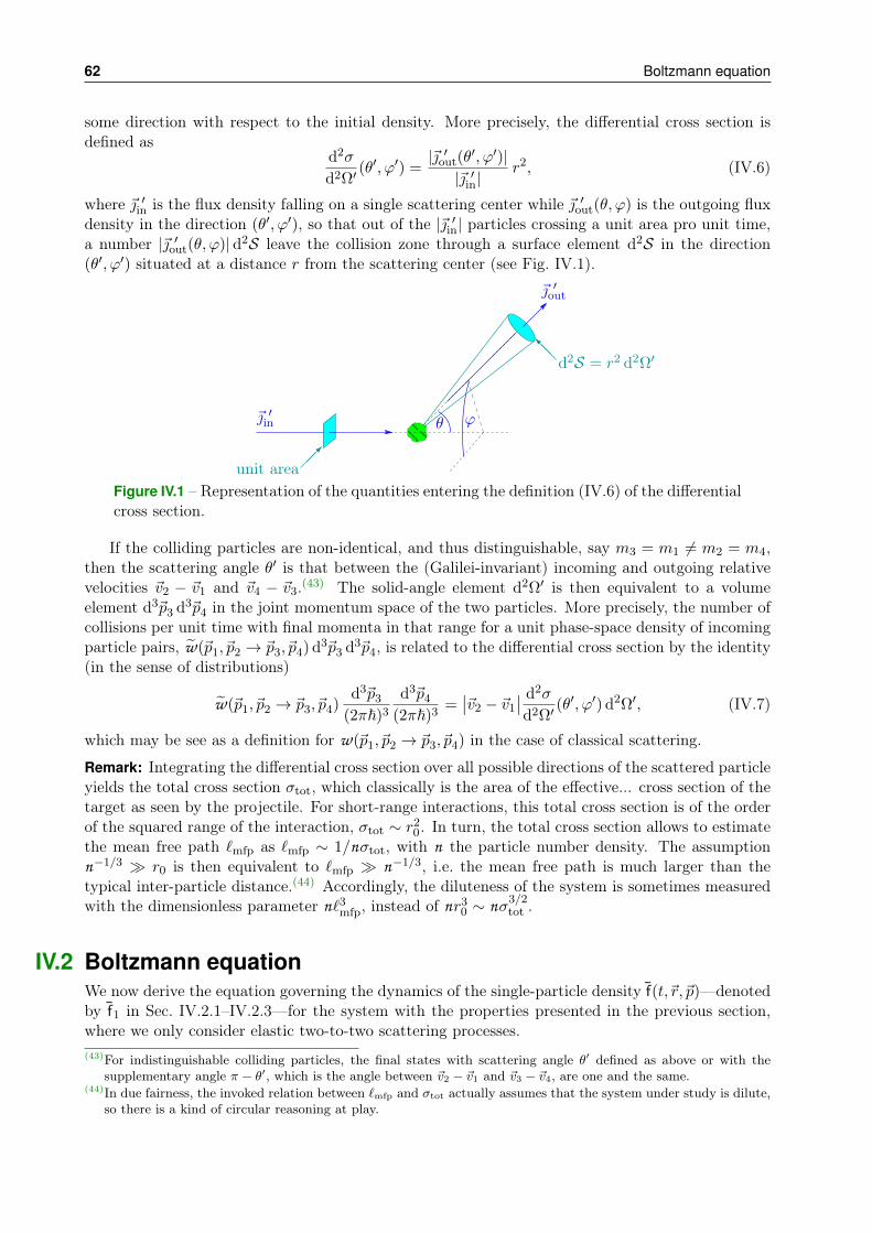
62 Boltzmann equation
some direction with respect to the initial density. More precisely, the differential cross section isdefined as
d2σ
d2Ω′(θ′, ϕ′) =
|~ ′out(θ′, ϕ′)|
|~ ′in|r2, (IV.6)
where ~ ′in is the flux density falling on a single scattering center while ~ ′out(θ, ϕ) is the outgoing fluxdensity in the direction (θ′, ϕ′), so that out of the |~ ′in| particles crossing a unit area pro unit time,a number |~ ′out(θ, ϕ)|d2S leave the collision zone through a surface element d2S in the direction(θ′, ϕ′) situated at a distance r from the scattering center (see Fig. IV.1).
θ ϕ~ ′in
~ ′out
@@Id2S = r2 d2Ω′
unit areaFigure IV.1 – Representation of the quantities entering the definition (IV.6) of the differentialcross section.
If the colliding particles are non-identical, and thus distinguishable, say m3 = m1 6= m2 = m4,then the scattering angle θ′ is that between the (Galilei-invariant) incoming and outgoing relativevelocities ~v2 − ~v1 and ~v4 − ~v3.(43) The solid-angle element d2Ω′ is then equivalent to a volumeelement d3~p3 d3~p4 in the joint momentum space of the two particles. More precisely, the number ofcollisions per unit time with final momenta in that range for a unit phase-space density of incomingparticle pairs, w(~p1,~p2 → ~p3,~p4) d3~p3 d3~p4, is related to the differential cross section by the identity(in the sense of distributions)
w(~p1,~p2 → ~p3,~p4)d3~p3
(2π~)3
d3~p4
(2π~)3=∣∣~v2 − ~v1
∣∣ d2σ
d2Ω′(θ′, ϕ′) d2Ω′, (IV.7)
which may be see as a definition for w(~p1,~p2 → ~p3,~p4) in the case of classical scattering.
Remark: Integrating the differential cross section over all possible directions of the scattered particleyields the total cross section σtot, which classically is the area of the effective... cross section of thetarget as seen by the projectile. For short-range interactions, this total cross section is of the orderof the squared range of the interaction, σtot ∼ r2
0. In turn, the total cross section allows to estimatethe mean free path `mfp as `mfp ∼ 1/nσtot, with n the particle number density. The assumptionn−1/3 r0 is then equivalent to `mfp n−1/3, i.e. the mean free path is much larger than thetypical inter-particle distance.(44) Accordingly, the diluteness of the system is sometimes measuredwith the dimensionless parameter n`3mfp, instead of nr3
0 ∼ nσ3/2tot .
IV.2 Boltzmann equationWe now derive the equation governing the dynamics of the single-particle density f(t,~r,~p)—denotedby f1 in Sec. IV.2.1–IV.2.3—for the system with the properties presented in the previous section,where we only consider elastic two-to-two scattering processes.(43)For indistinguishable colliding particles, the final states with scattering angle θ′ defined as above or with the
supplementary angle π − θ′, which is the angle between ~v2 − ~v1 and ~v3 − ~v4, are one and the same.(44)In due fairness, the invoked relation between `mfp and σtot actually assumes that the system under study is dilute,
so there is a kind of circular reasoning at play.

IV.2 Boltzmann equation 63
The derivation presented in this section is of a rather heuristic spirit, emphasizing the physicalmeaning of the terms on the right hand side of the Boltzmann equation. An alternative derivation,starting from the BBGKY hierarchy, is given in the appendix (IV.A) to this Chapter.
IV.2.1 General formulation
Since f1(t,~r,~p) is an instance of single-particle density—admittedly, on a coarse-grained versionof space-time, yet this makes no difference here—, its evolution equation could be derived in thesame manner as in the previous chapter III. Accordingly, in the absence of collisions f1 obeys thesingle-particle Liouville equation [cf. (III.15)]
∂ f1(t,~r,~p)
∂t+ ~v · ~∇~r f1(t,~r,~p) + ~F · ~∇~p f1(t,~r,~p) = 0.
This result can also be derived by counting particles within a volume d3~r d3~p around point (~r,~p)at time t, then by investigating where these particles are at a later time t+ dt, invoking Liouville’stheorem (II.15) to equate the new volume they occupy to the old one.(45)
Traditionally, the influence of collisions on the evolution is expressed by introducing a symboliccollision term (∂ f1/∂t)coll. in the right member
∂ f1
∂t+ ~v · ~∇~r f1 + ~F · ~∇~v f1 =
(∂ f1
∂t
)coll.
. (IV.8)
The role of the collision term is to describe the change induced by scatterings in the number ofparticles f1(t,~r,~p) d3~r d3~p inside an infinitesimal volume element around point (~r,~p).
The purpose of next subsection will be to give substance to this as yet empty notation. Inparticular, we shall split the collision term into a “gain term”—describing the particles that enterthe volume d3~r d3~p after a collision—and a “loss term”—corresponding to the particles which arescattered away from d3~r d3~p: (
∂ f1
∂t
)coll.
≡(∂ f1
∂t
)gain
−(∂ f1
∂t
)loss
. (IV.9)
Remark: In the same spirit as the right-hand side of Eq. (IV.8), one can designate the second andthird terms of the left member as the rates of change of f1 respectively caused by the motion of theparticles and by the external force:
∂ f1
∂t= −
(∂ f1
∂t
)motion
−(∂ f1
∂t
)force
+
(∂ f1
∂t
)coll.
. (IV.10)
IV.2.2 Computation of the collision term
We now derive the form of the two contributions to the collision term (IV.9), starting with theloss term.
:::::::IV.2.2 a
:::::::::::Loss term
Consider a volume element d3~r d3~p1 around a point (~r,~p1) at time t. A particle inside thisrange can scatter on a partner also situated at ~r—collisions are local—having a momentum ~p2 upto d3~p2. After the collision, the outgoing particles have momenta ~p3, ~p4, with a probability relatedto the transition rate w(~p1,~p2 → ~p3,~p4). Integrating over all possible final momenta yields thetotal scattering probability for initial particles with momenta ~p1, ~p2. Since d3~p1 is infinitesimallysmall, any scattering process will give both colliding particles a different final momentum, so thatany collision automatically leads to a decrease of the number of particles inside d3~p1.(45)This proof can for instance be found in Huang [33, Chap. 3.1] or Reif [35, Chap. 13.2].
64 Boltzmann equation
To obtain the number of particles which are scattered away from d3~p1, one has to multiply thetransition rate per unit volume for the collision of one pair of particles with momenta ~p1, ~p2 by thetotal number of particles 1 and 2 per unit volume in the respective momentum ranges at time t.Very generally, this number is given by(46)
f2(t,~r,~p1,~r,~p2) d3~rd3~p1
(2π~)3
d3~p2
(2π~)3,
with f2 the (coarse-grained) joint two-particle density. Eventually, one integrates over all possiblemomenta ~p2 of the partner, which yields, after dividing by d3~r d3~p1/(2π~)3(
∂ f1
∂t
)loss
(t,~r,~p1) =
∫f2(t,~r,~p1,~r,~p2)w(~p1,~p2 → ~p3,~p4)
d3~p2
(2π~)3
d3~p3
(2π~)3
d3~p4
(2π~)3. (IV.11a)
In terms of the differential cross section, this loss term reads(∂ f1
∂t
)loss
(t,~r,~p1) =
∫f(2)
(t,~r,~p1,~r,~p2)∣∣~v2 − ~v1
∣∣ d2σ
d2Ω′(θ′, ϕ′) d2Ω′
d3~p2
(2π~)3. (IV.11b)
Remark: The integrand of the latter expression (IV.11b) actually involves quantities measured indifferent rest frames: ~p1, ~p2 are with respect to the rest frame in which the system is studied, whileprimed quantities are in the respective centre-of-momentum frames of the binary collisions—which,for a fixed ~p1, depend on ~p2!
:::::::IV.2.2 b
:::::::::::Gain term
The gain term describes particles which at time t acquire the momentum ~p1 up to d3~p1 in thefinal state of a collision. We thus need to consider scattering processes ~p3,~p4 → ~p1,~p2, where thevalues of the initial momenta and of ~p2 are irrelevant and thus will be integrated over.
For fixed ~p3, ~p4 and for a given ~p2 known up to d3~p2, the number of particles with final momentain the proper range for a unit number density of incoming particles is given by [cf. Eq. (IV.4b)]
w(~p3,~p4 → ~p1,~p2)d3~p1
(2π~)3
d3~p2
(2π~)3.
Multiplying by the two-particle distribution f2(t,~r,~p3,~r,~p4), which gives the density of particleswith the respective momenta in the initial state, and integrating over these momenta as well asover the momentum ~p2 of the partner particle, one finds the number of “gained” particles per unitvolume(
∂ f1
∂t
)gain
(t,~r,~p1)d3~p1
(2π~)3=
d3~p1
(2π~)3
∫f2(t,~r,~p3,~r,~p4) w(~p3,~p4 → ~p1,~p2)
d3~p2
(2π~)3
d3~p3
(2π~)3
d3~p4
(2π~)3.
Dividing both sides by d3~p1/(2π~)3 and invoking the microreversibility property (IV.5c), this maybe recast as(
∂ f1
∂t
)gain
(t,~r,~p1) =
∫f2(t,~r,~p3,~r,~p4) w(~p1,~p2 → ~p3,~p4)
d3~p2
(2π~)3
d3~p3
(2π~)3
d3~p4
(2π~)3. (IV.12a)
Equivalently, one may write(∂ f1
∂t
)gain
(t,~r,~p1) =
∫f2(t,~r,~p3,~r,~p4)
∣∣~v2 − ~v1
∣∣ d2σ
d2Ω′(θ′, ϕ′) d2Ω′
d3~p2
(2π~)3, (IV.12b)
where relation (IV.7) was used.(46)The reader upset by the presence of the factor d3~r despite the fact that we are interested in the number of pairs
per unit volume may want to consider the number of pairs with both particles in the volume element d3~r, writingit first in the form
f2(t,~r,~p1,~r2,~p2) d3~r d3~r2d3~p1
(2π~)3d3~p2
(2π~)3
and then letting ~r2 = ~r—and accordingly d3~r2 = d3~r. The announced number of pairs per unit volume is thenobtained by dividing by (a single factor of) d3~r.

IV.2 Boltzmann equation 65
IV.2.3 Closure prescription: molecular chaos
Gathering the loss and gain terms (IV.11a) and (IV.12a) together, the collision term, or collisionintegral , in the right-hand side of the Boltzmann equation reads(
∂ f1
∂t
)coll.
(t,~r,~p1) =
∫ [f2(t,~r,~p3,~r,~p4)− f2(t,~r,~p1,~r,~p2)
]w(~p1,~p2 → ~p3,~p4)
d3~p2
(2π~)3
d3~p3
(2π~)3
d3~p4
(2π~)3,
(IV.13a)or equivalently [cf. Eqs (IV.11b) and (IV.12b)](
∂ f1
∂t
)coll.
(t,~r,~p1) =
∫ [f2(t,~r,~p3,~r,~p4)− f2(t,~r,~p1,~r,~p2)
]∣∣~v2 − ~v1
∣∣ d2σ
d2Ω′(θ′, ϕ′) d2Ω′
d3~p2
(2π~)3. (IV.13b)
As anticipated from the discussion of the BBGKY hierarchy in the previous chapter, the collisionintegral for the evolution of the single-particle density involves the two-particle density f2. In turn,one can derive the collision term for the dynamics of the latter, which depends on f3, and so forth.
Boltzmann’s proposal was to transform the collision integral (IV.13a) into a term involving f1
only, by invoking the assumption of molecular chaos, or Stoßzahlansatz, according to which thevelocities of the particles before the collision are uncorrelated
f2(t,~r,~p1,~r,~p2) = f1(t,~r,~p1) f1(t,~r,~p2) before a collision at instant t. (IV.14)
Just after a collision, two particles which have scattered on each other are correlated—invertingtheir velocities, one makes them collide, which is a rare event. Yet before they meet and collideagain, they will undergo many scatterings with other, random particles, which wash out any traceof this correlation, and justifies the above assumption.
Remark: Molecular chaos is thus a weaker assumption that the factorization (III.23) in the Vlasovequation, which holds at any instant and for all positions of the two particles.
Under this assumption and inserting the resulting collision integral in the right-hand side ofEq. (IV.8), one obtains the Boltzmann kinetic equation(47)
∂ f(t,~r,~p1)
∂t+ ~v1 · ~∇~r f(t,~r,~p1) + ~F · ~∇~p1 f(t,~r,~p1) =(
1− δ1,2
2
)∫ [f(t,~r,~p3)f(t,~r,~p4)− f(t,~r,~p1)f(t,~r,~p2)
]w(~p1,~p2 → ~p3,~p4)
d3~p2
(2π~)3
d3~p3
(2π~)3
d3~p4
(2π~)3,
(IV.15a)
where the prefactor 1− δ1,2/2 was introduced to ensure that the formula also holds without doublecounting when particles 1 and 2 are identical (in which case δ1,2 = 1, otherwise is δ1,2 = 0).Equivalently, the Boltzmann equation may recast as
∂ f(t,~r,~p1)
∂t+ ~v1 · ~∇~r f(t,~r,~p1) + ~F · ~∇~p1 f(t,~r,~p1) =(
1− δ1,2
2
)∫ [f(t,~r,~p3)f(t,~r,~p4)− f(t,~r,~p1)f(t,~r,~p2)
]∣∣~v2 − ~v1
∣∣ d2σ
d2Ω′(θ′, ϕ′) d2Ω′
d3~p2
(2π~)3.
(IV.15b)
Remarks:
∗ One often introduces the abbreviations f(1) ≡ f(t,~r,~p1), f(2) ≡ f(t,~r,~p2), and so on, so that thecollision integral is shortly written as(47)From now on, we drop the notation f1 and only use f.

66 Boltzmann equation
(∂ f(1)
∂t
)coll.
=
∫ [f(3)f(4)− f(1)f(2)
]w(~p1,~p2 → ~p3,~p4)
d3~p2
(2π~)3
d3~p3
(2π~)3
d3~p4
(2π~)3. (IV.15c)
To shorten expressions further, we shall also use∫~pi
≡∫
d3~pi(2π~)3
, leading for instance to(∂ f(1)
∂t
)coll.
=
∫~p2
∫~p3
∫~p4
[f(3)f(4)− f(1)f(2)
]w(~p1,~p2 → ~p3,~p4). (IV.15d)
∗ The generalization of the Boltzmann equation to the case of a mixture of substances is straight-forward: in the collision term for the evolution of the position-velocity-space density of a component,one has to sum the contribution from the (elastic two-to-two) scattering processes of the particles ofthat substance with each other—taking into account the 1
2 factor to avoid double-counting—, andthe contributions from collisions with particles of other components.
IV.2.4 Phenomenological generalization to fermions and bosons
The collision term of the Boltzmann equation can easily be modified so as to accommodate thePauli exclusion principle between particles with half-integer spins.(48) Considering the two-to-twocollision ~pi,~pj → ~pk,~pl, where all particles are fermions,(at) the “repulsive” behavior of the latter canbe phenomenologically accounted for by preventing the scattering process to happen when one of thefinal states ~pk or ~pl is already occupied. That is, one postulates that the rate for the process is notonly proportional to the product f(i)f(j) of the phase-space densities of the initial particles—wherewe use the same shorthand notation as in Eq. (IV.15c)—, but also to the product [1− f(k)][1− f(l)]involving the densities of the final state particles. The collision integral of the Boltzmann equationthus reads(∂ f(1)
∂t
)coll.
=
∫~p2
∫~p3
∫~p4
(f(3)f(4)
[1− f(1)
][1− f(2)
]− f(1)f(2)
[1− f(3)
][1− f(4)
])w(~p1,~p2 → ~p3,~p4).
(IV.16)A similar generalization, which simulates the “attractive” character of bosons,(au) consists in
enhancing the rate of the process ~pi,~pj → ~pk,~pl, when there are already particles in the final state.This is done by multiplying the rate by the factor [1 + f(k)][1 + f(l)], which yields(∂ f(1)
∂t
)coll.
=
∫~p2
∫~p3
∫~p4
(f(3)f(4)
[1 + f(1)
][1 + f(2)
]− f(1)f(2)
[1 + f(3)
][1 + f(4)
])w(~p1,~p2 → ~p3,~p4).
(IV.17)We shall see below that these seemingly ad hoc generalizations (IV.16)–(IV.17) lead for instance tothe proper equilibrium distributions.
An issue is naturally the actual meaning of f in the generalized kinetic equations obtained withthe above collision terms, since phase space is usually not considered as an interesting concept inquantum mechanics, where the Heisenberg uncertainties prevent a particle from being localizedat a well-defined point in µ-space.
IV.2.5 Additional comments and discussions
Now that we have established the actual form of the Boltzmann equation, especially of itscollision term, we wish to come back to the assumptions made in Sec. IV.1.1, to discuss their rolein a new light.(48)This idea seems to date back to Landau, in his work on the theory of Fermi liquids [36].(at)E. Fermi, 1901–1954 (au)S. N. Bose, 1894–1974

IV.3 Balance equations derived from the Boltzmann equation 67
An important point is the coarse graining of both time and position space. Thanks to it, themomenta of the colliding particles skip instantaneously from their initial values ~p1, ~p2 to the finalones, without going through intermediate values as would happen otherwise—except in the unreal-istic case when the particles are modelled as hard spheres. If this transition were not instantaneous,particle 1—a similar reasoning holds for the other colliding particle (2), as well as for particles 3and 4 in the gain term—would at the time t of the collision no longer have the momentum ~p1 ithad “long” before the scattering. Accordingly, the distribution of particle 1 in the loss part of thecollision integral should not be f(t,~r,~p1), but rather one of the following possibilities:
• f evaluated at time t, yet for the position ~r ′1 and momentum ~p ′1 of particle 1 at that veryinstant: in a classical description of the scattering process, ~r ′1 and ~p ′1 depend for instance onthe impact parameter of the collision; whereas they are not even well-defined in a quantummechanical description.
• f evaluated at momentum ~p1, yet at a time t− τ , before the collision, at which particle 1 stillhad this momentum, and accordingly at some position ~r1 6= ~r.
In the former case, one loses the locality in position space, while in the latter one has to abandonlocality both in time and space. The advantage of adopting a coarse-grained description is thus toprovide an evolution equation which is local both in t and ~r, as is the case of Eq. (IV.15).
Thanks to the time locality of the Boltzmann equation, the evolution of f is “Markovian” in thewide sense of Sec. I.2.1, i.e. its rate of change is memoryless and only depends on f at the sameinstant.
Another assumption is that the time scale on which the coarse graining is performed is muchsmaller than the average duration between two successive collisions of a particle, and similarly thatthe spatial size of the coarse-grained cells is much smaller than the mean free path. This allowsone to meaningfully treat f as a continuous—and even differentiable—function of t and ~r, and thusamounts to assuming that the system properties do not change abruptly in time or spatially.
Eventually, one can note that the molecular chaos assumption (IV.14) provides a closed equationfor f, yet at the cost of introducing nonlinearity, whereas the successive equations of the BBGKYhierarchy (III.14) are all linear.
IV.3 Balance equations derived from the Boltzmann equationWe now investigate various balance equations that hold in a system obeying the Boltzmann equation,beginning with conservation laws, then going on with the celebrated H-theorem. Motivated by thistheorem, we then define various equilibrium distributions.
IV.3.1 Conservation laws
:::::::IV.3.1 a
:::::::::::::::::::::::::::::::::::Properties of the collision integral
Let Icoll.(1, 2, 3, 4) denote the integrand of the collision integral on the right-hand side of theBoltzmann equation (IV.15): (
∂ f(1)
∂t
)coll.
=
∫~p2
∫~p3
∫~p4
Icoll.(1, 2, 3, 4) (IV.18a)
withIcoll.(1, 2, 3, 4) ≡
[f(3)f(4)− f(1)f(2)
]w(~p1,~p2 → ~p3,~p4) (IV.18b)
in the case of “classical” particles—the expression in the case of fermions resp. bosons can be readat once off Eq. (IV.16) resp. (IV.17).

68 Boltzmann equation
This integrand obeys various properties that appear when the role of the particles are exchanged,irrespective of whether they are indistinguishable or not.
• (S) The integrand in the collision term of the Boltzmann equation is symmetric under theexchanges ~p1 ↔ ~p2 and ~p3 ↔ ~p4.
This symmetry is trivial.
• (A) The integrand in the collision term of the Boltzmann equation is antisymmetric under thesimultaneous exchanges of ~p1, ~p2 with ~p3, ~p4.
This property is straightforward when one considers on the one hand the (mathematical)change of labels 1↔ 3, 2↔ 4, which gives a minus sign, and on the other hand the physicalmicroreversibility property encoded in Eq. (IV.5c).
Let χ(t,~r,~p) denote a collisional invariant , i.e. a microscopic quantity which is conserved inevery binary collision. Examples are particle number, linear momentum, or kinetic energy since thecollisions are elastic: the quantity can thus be scalar or vectorial. One then has the general identity∫
χ(t,~r,~p)
(∂ f
∂t
)coll.
(t,~r,~p)d3~p
(2π~)3= 0. (IV.19)
Let us use the notations f(1), f(2), . . . as in Eq. (IV.15c), and accordingly χ(1) ≡ χ(t,~r,~p1),χ(2) ≡ χ(t,~r,~p2), and so on. Using Eq. (IV.18a) then gives∫
~p1
χ(1)
(∂ f(1)
∂t
)coll.
=
∫~p1
∫~p2
∫~p3
∫~p4
χ(1)Icoll.(1, 2, 3, 4).
Exchanging first the dummy labels 1 and 2 of the integration variables, and invoking then thesymmetry property (S) of the integrand of the collision term, one finds∫
~p1
χ(1)
(∂ f(1)
∂t
)coll.
=
∫~p2
χ(2)
∫~p1
∫~p3
∫~p4
Icoll.(2, 1, 3, 4) =
∫~p1
∫~p2
∫~p3
∫~p4
χ(2)Icoll.(1, 2, 3, 4).
Combining the previous two equations, we may thus write∫~p1
χ(1)
(∂ f(1)
∂t
)coll.
=1
2
∫~p1
∫~p2
∫~p3
∫~p4
[χ(1) + χ(2)
]Icoll.(1, 2, 3, 4).
Invoking now the antisymmetry (A) after exchanging the dummy indices 1↔ 3 and 2↔ 4, oneobtains∫
~p1
χ(1)
(∂ f(1)
∂t
)coll.
=
∫~p3
χ(3)
∫~p1
∫~p2
∫~p4
Icoll.(3, 4, 1, 2) = −∫~p1
∫~p2
∫~p3
∫~p4
χ(3)Icoll.(1, 2, 3, 4).
Similarly the exchange 1↔ 4 and 2↔ 3 yields:∫~p1
χ(1)
(∂ f(1)
∂t
)coll.
=
∫~p4
χ(4)
∫~p1
∫~p2
∫~p4
Icoll.(4, 3, 2, 1) = −∫~p1
∫~p2
∫~p3
∫~p4
χ(4)Icoll.(1, 2, 3, 4).
Both previous lines lead to∫~p1
χ(1)
(∂ f(1)
∂t
)coll.
= −1
2
∫~p1
∫~p2
∫~p3
∫~p4
[χ(3) + χ(4)
]Icoll.(1, 2, 3, 4).
Gathering all intermediate results, there eventually comes∫~p1
χ(1)
(∂ f(1)
∂t
)coll.
=1
4
∫~p1
∫~p2
∫~p3
∫~p4
[χ(1) + χ(2)− χ(3)− χ(4)
]Icoll.(1, 2, 3, 4) = 0,
where the last identity comes from the local conservation property χ(1) + χ(2) = χ(3) + χ(4)expressing the invariance of χ under binary collisions. 2
We can now replace χ by various conserved quantities.
IV.3 Balance equations derived from the Boltzmann equation 69
:::::::IV.3.1 b
:::::::::::::::::::::::::::::::Particle number conservation
As already mentioned, the (local) particle number density is the integral over momenta of thephase space distribution
n(t,~r) ≡∫~p
f(t,~r,~p). (IV.20a)
On the other hand, the particle-number flux density is naturally given by
~JN (t,~r) ≡∫~p
f(t,~r,~p)~v, (IV.20b)
where each “phase-space cell” contributes with its velocity ~v, weighted with the corresponding dis-tribution.
Integrating now the Boltzmann equation (IV.8) over ~p, and exchanging the order of the deriva-tives with respect to time or space and of the integral over velocities, the first term in the left-handside gives ∂n/∂t, the second term equals ~∇~r · ~JN , while the third gives a vanishing contributionsince f vanishes at the boundaries of velocity space, to ensure the convergence of the integral in thenormalization condition (III.2a). In turn, considering identity (IV.19) with the collisional invariantχ = 1, the integral over ~p of the collision term vanishes. All in all, one obtains the local conservationlaw
∂n(t,~r)
∂t+ ~∇ · ~JN (t,~r) = 0, (IV.20c)
where we have dropped the now unnecessary subscript ~r on the gradient. This relation, known ascontinuity equation, is obviously of the general type (I.18). The immense progress is that n and~JN can now be computed starting from a microscopic theory—if f is known!—, instead of beingpostulated at the macroscopic level.
:::::::IV.3.1 c
::::::::::::::::::::::Energy conservation
As a second application, we can consider the collisional invariant χ(t,~r,~p) = ~p 2/2m, i.e. thekinetic energy.(49) We introduce the local kinetic-energy density
ekin.(t,~r) =
∫~p
f(t,~r,~p)~p 2
2m(IV.21a)
and the local kinetic-energy flux density
~JEkin.(t,~r) =
∫~p
f(t,~r,~p)~p 2
2m~v. (IV.21b)
We first assume for simplicity that there is no external force acting on the particles.Multiplying each term of the Boltzmann equation by ~p 2/2m and integrating over velocity, one
finds the local conservation law
∂ekin.(t,~r)
∂t+ ~∇ · ~JEkin.
(t,~r) = 0, (IV.21c)
where identity (IV.19) has again been used.
(49). . . in the case of neutral particles.

70 Boltzmann equation
In the presence of an external force ~F independent from the particle momentum, a straight-forward integration by parts shows that there comes an extra term—the integral over velocity of~F ·~v multiplied by f(t,~r,~p)—, with a + sign if it is written as right-hand side of Eq. (IV.21c). Thistrivially corresponds to the work exerted by the external force per unit time.
Remarks:
∗ Alternatively, one can take for χ the sum of the kinetic energy ~p 2/2m and the potential energydue to the external force. The resulting balance equation is then the local conservation of totalenergy, of the type (IV.21c) with different energy density and flux density, even in the presence ofthe external force.
∗ As already noted in Sec. IV.1.2, the conservation of kinetic energy alone is conserved is relatedto the assumption of a weakly-interacting system, in which the relative amount of potential energyis small.
:::::::IV.3.1 d
:::::::::::::::::::::Momentum balance
Eventually, let χ be the i-th component pi of linear momentum. Let
~v(t,~r) ≡ 1
n(t,~r)~JN (t,~r) =
1
mn(t,~r)
∫~p
f(t,~r,~p)~p (IV.22a)
be the local flow velocity and
(J~P)ij
(t,~r) =1
n(t,~r)
∫~p
f(t,~r,~p) pi vj (IV.22b)
the j-th component of the local flux density of the i-th component of linear momentum.By integrating the Boltzmann equation multiplied by pi over momentum, one easily finds
∂[mn(t,~r)vi(t,~r)]
∂t+
3∑j=1
∂
∂xj[n(t,~r)
(J~P)ij
(t,~r)]
= n(t,~r)F i, (IV.22c)
which describes the rate of change of linear momentum under the influence of a force.The property (IV.19) and the balance equations (IV.20)–(IV.22) will be recast in a different formin Sec. IV.6.1 below.
Remark: Inspecting Eqs. (IV.20b) and (IV.22a), one recognizes that the „local flow velocity“ isactually the average local velocity of particles, i.e. it is related to particle flow. In a relativistictheory, where particle number is not conserved—the corresponding scalar conserved quantity israther a quantum number, like e.g. electric charge or baryon number—one may rather choose (afterLandau) to define the flow velocity as the velocity derived from the flux of energy.
IV.3.2 H-theorem
A further consequence of the properties of the collision integral is the so-calledH-theorem, whichdates back to Boltzmann himself.
Given a solution f(t,~r,~p) of the Boltzmann equation, a macroscopic quantity H(t) is definedby(50)
H(t) ≡∫
f(t,~r,~p) ln f(t,~r,~p) d6V , (IV.23)
(50)H(t) is not to be confused with the Hamilton function of the system. . .
IV.3 Balance equations derived from the Boltzmann equation 71
with d6V ≡ d3~r d3~p/(2π~)3 the measure on the (coarse-grained) single-particle phase space, asdefined in Eq. (II.4b).
One also defines a related quantity, which we shall for the time being without further justificationcall Boltzmann entropy , as
SB(t) ≡ kB∫
f(t,~r,~p)[1− ln f(t,~r,~p)
]d6V , (IV.24)
with kB the Boltzmann constant.We can check at once the simple relation
SB(t) = −kBH(t) + constant, (IV.25)
where the unspecified constant is actually simply related to the total number of particles.
Remark: When adopting the generalizations (IV.16)–(IV.17) of the collision integral to fermions orbosons, one should accordingly modify the expressions of H(t) and SB(t). For instance, one shouldconsider
H(t) ≡∫
f(t,~r,~p) ln f(t,~r,~p)±[1∓ f(t,~r,~p)
]ln[1∓ f(t,~r,~p)
]d6V , (IV.26)
where the upper (resp. lower) sign holds for fermions resp. bosons.
We can now turn to the H-theorem, which states that if just before a given time t0 the sys-tem under study obeys the Boltzmann equation—and in particular fulfills the molecular chaosassumption—, then H(t) decreases at time t0
dH(t)
dt≤ 0. (IV.27)
There ensues at once that the Boltzmann entropy is increasing
dSB(t)
dt≥ 0. (IV.28)
The proof of the H-theorem relies again on the properties of the collision integral. First, astraightforward differentiation yields, after exchanging the order of time derivative and integrationover position and velocity,
dH(t)
dt=
∫∂
∂t
[f(t,~r,~p) ln f(t,~r,~p)
]d6V =
∫∂ f(t,~r,~p)
∂t
[1 + ln f(t,~r,~p)
]d6V .
Since f is a solution to the Boltzmann equation, the partial derivative ∂ f/∂t can be rewritten withthe help of Eq. (IV.8). The integral over ~r of the term ~v · ~∇~r f yields the difference of the values of fat the boundaries of position space, where f vanishes, so that the corresponding contribution is zero.The same reasoning and result hold for the integral over ~p of the term proportional to ~∇~p f—this istrivial if the force is velocity independent, and still holds when ~F depends on ~v. All in all, one thusquickly finds
dH(t)
dt=
∫ (∂ f
∂t
)coll.
(t,~r,~p)[1 + ln f(t,~r,~p)
]d6V . (IV.29)
This shows that H(t) does not evolve in the absence of collision: the decrease in H(t) is entirelydue to the scattering processes.
To deal with the remaining integral in Eq. (IV.29), one can first use property (IV.19) with χ = 1,to get rid of the constant 1 in the angular brackets of the integrand. We are then left with
dH(t)
dt=
∫ (∂ f
∂t
)coll.
(t,~r,~p) ln f(t,~r,~p) d6V =
∫ [ ∫~p1
(∂ f(1)
∂t
)coll.
ln f(1)
]d3~r,

72 Boltzmann equation
where the second identity follows from renaming the integration variable ~p as ~p1 and using theshorthand notations already introduced in the previous section.
As in the proof of relation (IV.19) one can find by writing explicitly the collision integral interms of its integrand and using the symmetry properties of the latter and the change of labels1↔ 2 the identities∫
~p1
(∂ f(1)
∂t
)coll.
ln f(1) =
∫~p1
∫~p2
∫~p3
∫~p4
Icoll.(1, 2, 3, 4) ln f(1) =
∫~p2
∫~p1
∫~p3
∫~p4
Icoll.(2, 1, 3, 4) ln f(2)
=
∫~p1
∫~p2
∫~p3
∫~p4
Icoll.(1, 2, 3, 4) ln f(2)
=1
2
∫~p1
∫~p2
∫~p3
∫~p4
Icoll.(1, 2, 3, 4)[
ln f(1) + ln f(2)].
Similarly one finds∫~p1
(∂ f(1)
∂t
)coll.
ln f(1) = −∫~p1
∫~p2
∫~p3
∫~p4
Icoll.(1, 2, 3, 4) ln f(3) = −∫~p2
∫~p1
∫~p3
∫~p4
Icoll.(1, 2, 3, 4) ln f(4)
= −1
2
∫~p1
∫~p2
∫~p3
∫~p4
Icoll.(1, 2, 3, 4)[
ln f(3) + ln f(4)].
This eventually gives
dH(t)
dt=
1
4
∫ ∫~p1
∫~p2
∫~p3
∫~p4
Icoll.(1, 2, 3, 4)[
ln f(1) + ln f(2)− ln f(3)− ln f(4)]
d3~r.
Replacing the integrand of the collision integral by its expression (IV.18b) and performing somestraightforward algebra, one obtains
dH(t)
dt=
1
4
∫ ∫~p1
∫~p2
∫~p3
∫~p4
[f(3)f(4)− f(1)f(2)
]w(~p1,~p2 → ~p3,~p4) ln
f(1)f(2)
f(3)f(4)
d3~r
=1
4
∫ ∫~p1
∫~p2
∫~p3
∫~p4
f(3)f(4)
[1− f(1)f(2)
f(3)f(4)
]ln
f(1)f(2)
f(3)f(4)w(~p1,~p2 → ~p3,~p4)
d3~r. (IV.30)
Now, the integrand is always negative—since (1 − x) lnx ≤ 0 for all x, while all other factors arepositive—, which proves the H-theorem. 2
Remarks:
∗ Boltzmann’s contemporaries strongly objected to his ideas, and in particular to the H theorem,due to their incomplete understanding of its content. One of the objections was that the assumedinvariance of interactions under time reversal, combined with the invariance of the equations ofmotion (for instance the Hamilton equations or the Liouville equation) under time reversal, shouldlead to the equivalence of both time directions, while the H-theorem selects a time direction.
The answer to this apparent paradox is that H(t) is not decreasing at any time, but only whenthe system satisfies the assumption of molecular chaos. Actually, the existence of a preferred timedirection was somehow postulated from the beginning by Boltzmann, when he made the differencebetween the state of the system before a collision (molecular chaos, the particles are uncorrelated)and after (the particles are then correlated). There is thus no inconsistency if H(t) distinguishesbetween both time directions.
∗ Defining the quantitiesh(t,~r) ≡
∫~p
f(t,~r,~p) ln f(t,~r,~p), (IV.31a)
~JH(t,~r) ≡∫~p~v f(t,~r,~p) ln f(t,~r,~p), (IV.31b)
IV.4 Solutions of the Boltzmann equation 73
and
σH(t,~r) ≡∫~p
(∂ f
∂t
)coll.
(t,~r,~p)[1 + ln f(t,~r,~p)
]=
∫~p
(∂ f
∂t
)coll.
(t,~r,~p) ln f(t,~r,~p), (IV.31c)
one easily finds that they obey the local balance equation
∂h(t,~r)
∂t+ ~∇ · ~JH(t,~r) = σH(t,~r), (IV.31d)
which suggests the interpretation of h, JH and σH as density, flux density and source density(51) ofthe H-quantity, respectively.
IV.4 Solutions of the Boltzmann equationWe now turn to a discussion of the solution of the Boltzmann equation.
IV.4.1 Equilibrium distributions
According to theH-theorem,H(t) is a decreasing function of time—at least when the assumptionof molecular chaos holds. Besides, the defining formula (IV.23) shows that H(t) is bounded frombelow when the spatial volume V occupied by the system, and accordingly its total energy, is finite.
This follows from the finiteness of the available phase space—the finite energy of the systemtranslates into an upper bound on momenta—and the fact that the product x lnx is alwayslarger than −1/e.
As a consequence, H(t) converges in the limit t→∞, i.e. its derivative vanishes:
dH(t)
dt= 0 (IV.32)
or equivalently dSB(t)/dt = 0. In this section, we define and discuss two types of distributions thatfulfill this condition:
• the global equilibrium distribution feq.(~r,~p) is defined as a stationary solution of the Boltzmannequation
∂ feq.
∂t= 0 (IV.33)
obeying Eq. (IV.32). In that case, the system has reached global thermodynamic equilibrium,with uniform values of the temperature T and of the average velocity ~v of particles, as well asof their number density n (or equivalently the chemical potential µ) when there is no externalforce. In particular, feq. cancels the collision integral (IV.15c).
• local equilibrium distributions, hereafter denoted as f(0)
(t,~r,~p), cancel the collision term of theBoltzmann equation—and thereby obey condition (IV.32)—, yet are in general not solutionsto the whole equation itself.
In practice, an out-of-equilibrium system first tends, under the influence of collisions alone, towardsa state of local equilibrium. In a second step, the interplay of collisions and the drift terms drivesthe system towards global equilibrium.
Remarks:∗ If the spatial volume occupied by the system is unbounded, then H resp. SB is not necessarilybounded from below resp. above, and thus a state of global equilibrium may never be reached. Thisis for instance the case for a collection of particles expanding initially confined into a small regionof space left free to expand into the vacuum.(51)In this case it might be more appropriate to call it sink density, since H(t) is decreasing.
74 Boltzmann equation
∗ Even if the system is confined in a finite volume, it may still be “stuck” in a persistent non-equilibrium setup. An example is that of a gas performing undamped “monopole” oscillationsin a spherically symmetric harmonic trap, as studied theoretically e.g. in Ref. [37] and realizedexperimentally (to a good approximation) with cold 87Rb atoms [38].
:::::::IV.4.1 a
::::::::::::::::::::Global equilibrium
For simplicity, we begin with the case when the system is homogeneous and there is no exter-nal force. Consistency then implies that the distribution function f is independent of ~r. This inparticular holds for the equilibrium distribution, feq.(~p), and the corresponding particle density n .
Inspecting the derivative (IV.30), one sees that the equilibrium condition dH(t)/dt = 0 can onlybe fulfilled if the always-negative integrand is actually vanishing itself, which implies the identity
feq.(~p1)feq.(~p2) = feq.(~p3)feq.(~p4),
for every quadruplet (~p1,~p2,~p3,~p4) satisfying the kinetic-energy- and momentum-conservation re-lationships (IV.3) and allowed by the requirements on the system, in case the latter has a finiteenergy. From now on we assume that feq. is everywhere non-zero.(52) Taking the logarithm of theabove relation gives
ln feq.(~p1) + ln feq.(~p2) = ln feq.(~p3) + ln feq.(~p4),
which expresses that ln feq.(~p) is a quantity conserved in any elastic two-to-two collision, and isthus a linear combination of additive collision invariants χ(~p). Assuming that particle number—amounting to χ(~p) = 1—, momentum [χ(~p) = ~p] and kinetic energy [χ(~p) = ~p 2/2m] form a basis ofthe latter,(53) one can write ln feq.(~p) = A′ + ~B ′ · ~p+ C ′~p 2, with constant A′, ~B ′, C ′. Equivalently,one has (with new, related constants A, C and ~p0)
feq.(~p) = C e−A(~p−~p0)2 . (IV.34)
Following relation (IV.2), the momentum-space integral of feq.(~p) should yield the particle numberdensity n , which necessitates C = (4π~2A)3/2n . The integral of the product feq.(~p)~p with feq. of theform (IV.34) over the whole phase space then gives ~p0, which should equal the total momentumof the particles; the latter vanishes if the particles are studied in their global rest frame, yielding~p0 = ~0. Eventually, the momentum-space integral of feq.(~p)~p
2/2m should give n times the averagekinetic energy per particle, while Eq. (IV.34), together with the relation between C and A foundabove, leads to 3n/4mA. Denoting the average kinetic energy per particle by 3
2kBT , one thus findsA = 1/2mkBT . All in all, one obtains
feq.(~p) = n(
2π~2
mkBT
)3/2
e−~p2/2mkBT , (IV.35)
which is the Maxwell(av)–Boltzmann distribution.(54)
One easily checks that the latter actually also cancels the left-hand side of the Boltzmannequation in the absence of external force, i.e. it represents the global equilibrium distribution.
(52)The identically vanishing distribution f ≡ 0 is clearly stationary and does fulfill condition (IV.32), yet it of courseleads to a vanishing particle number, i.e. it represents a very boring system!
(53)A proof was given by Grad [39], which is partly reproduced by Sommerfeld [40, § 42]. An alternative argumentis that if there were yet another kinematic collisional invariant in two-to-two scatterings, it would yield a fifthcondition on the outgoing momenta—the requirement of having two particles in the final state leaves the constraintsfrom energy and momentum conservation—, and thus restrict their angles, which is not the case.
(54)possibly up to the normalization factor, since in these lecture notes f is dimensionless and normalized to the totalnumber of particles, while the “usual” Maxwell–Boltzmann distribution is rather a probability distribution.
(av)J. C. Maxwell, 1831–1879

IV.4 Solutions of the Boltzmann equation 75
Remark: The Maxwell–Boltzmann distribution (IV.35) was probably known to the reader as thesingle-particle phase-space distribution of a classical ideal monoatomic gas at thermodynamic equi-librium studied in the canonical ensemble. Here it emerges as the (almost) universal long-time limitof the out-of-equilibrium evolution of a Boltzmann gas, in which the average energy per particle was“arbitrarily” denoted by 3
2kBT , where T has no other interpretation. This constitutes a totally dif-ferent vision, yet the fact that both approaches yield the same distribution hints at the consistencyof their results.
In case the system is subject to an external force deriving from a time-independent scalarpotential, ~F = −~∇V (~r), the stationary equilibrium solution of the Boltzmann equation is no longerspatially homogeneous, but becomes
feq.(~r,~p) = n(~r)
(2π~2
mkBT
)3/2
e−~p2/2mkBT with n(~r) ≡ N e−V (~r)/kBT∫
e−V (~r)/kBT d3~r
. (IV.36)
Boltzmann entropy of the global equilibrium distributionInserting the equilibrium distribution (IV.36) into the Boltzmann entropy (IV.24), one finds with
the help of Eq. (A.1c)
SB = NkB ln
[VN
(mkBT
2π~2
)3/2]+
5
2NkB, (IV.37)
where V is the volume occupied by the particles. This result coincides with the Sackur (aw)–Tetrode(ax) formula [41, 42] for the thermodynamic entropy of a classical ideal gas under the sameconditions. This shows that at equilibrium the Boltzmann entropy, which is also defined out ofequilibrium, coincides with the thermodynamic entropy.
:::::::IV.4.1 b
:::::::::::::::::::Local equilibrium
A non-equilibrated macroscopic system of weakly-interacting classical particles will not reachthe global equilibrium distribution (IV.35) at once, the approach to equilibrium can be decomposedin “successive” (not in a strict chronological sense, but rather logically) steps involving various timescales [cf. Eqs. (III.16), (III.17)]:
i. Over the shortest time scale τc, neighbouring particles scatter on each other. These collisions—which strictly speaking are not described by the Boltzmann equation—lead to the emergenceof molecular chaos.
ii. Once molecular chaos holds, scatterings tend to drive the system to a state of local equilibrium,described by local thermodynamic variables as defined in chapter I: particle number densityn(t,~r), temperature T (t,~r) and average particle velocity ~v(t,~r). That is, the single-particledistribution f relaxes to a local equilibrium distribution, of the form
f(0)
(t,~r,~p) = n(t,~r)
[2π~2
mkBT (t,~r)
]3/2exp
−[~p−m~v(t,~r)
]22mkBT (t,~r)
, (IV.38)
which cancels the collision integral on the right-hand side of the Boltzmann equation. Thisrelaxation takes place over a time scale τr, which physically should be (much) larger than τc
since it involves “many” local scatterings.
iii. Eventually, the state of local equilibrium relaxes to that of global equilibrium over the timescales τs, τe defined in Eq. (III.16). This step in the evolution of the single-particle distributionf, which is now rather driven by the slow drift terms on the left-hand side of the Boltzmann
(aw)H. M. Sackur, 1895–1931 (ax)O. Tetrode, 1880–1914
76 Boltzmann equation
equation, is more conveniently described in terms of the evolution of local thermodynamicquantities obeying macroscopic equations, in particular those of hydrodynamics, as will bedescribed in Sec. IV.6.
Remark: In general, the distribution (IV.38) does not cancel the left-hand side of the Boltzmannequation and is thus not a solution of the equation. This is however not a problem, since thesingle-particle distribution f never really equals a given f
(0), it only tends momentarily towards it:the three steps which above have been described as successive actually take place simultaneously.
:::::::IV.4.1 c
::::::::::::::::::::::::::::::::::::::::::::::::::::Equilibrium distributions for bosons and fermions
The kinetic equations with a collision integral which simulates either the Pauli(ay) principleof particles with half-integer spin [Eq. (IV.16)] or the “gregariousness” of particles with integerspin [Eq. (IV.17)] also obey an H-theorem, and thus tend at large time to respective stationaryequilibrium distributions f
Feq. and f
Beq..
Repeating a reasoning analogous to that in paragraph IV.4.1 a, with feq. replaced by fFeq./(1− f
Feq.)
or fBeq./(1 + f
Beq.), one finds after some straightforward algebra
fFeq.(~p) =
1
CF exp(~p 2/2mkBT ) + 1(IV.39a)
and
fBeq.(~p) =
1
CB exp(~p 2/2mkBT )− 1, (IV.39b)
with CF, CB two constants ensuring the proper normalization of the distributions. These arerespectively the Fermi–Dirac and Bose–Einstein distributions as found within equilibrium statisticalmechanics for ideal quantum gases.
IV.4.2 Approximate solutions
The Boltzmann equation (IV.15) identifies the rate of change of the single-particle distributionf(t,~r,~p) to a collision integral, which accounts for microscopic two-body elastic collisions. It is a non-linear partial integro-differential equation, and as thus especially difficult to solve. Accordingly, fewexact solutions—apart from the equilibrium Maxwell–Boltzmann distribution (IV.35)–(IV.36)—areknown analytically. Instead, one has to resort to approximate solutions, based on various schemes,two of which are shortly presented here.
:::::::IV.4.2 a
::::::::::::::::::::::Orders of magnitude
As already mentioned in § III.2.2 b–III.2.2 c, the various terms of the Boltzmann equation a prioriinvolve different time or length scales. Introducing the typical size fc of f (at a given momentum),one may introduce characteristic times τevol., τs, τe, and τcoll. such that the dimensionless terms
τevol.
fc
∂ f
∂t,
τs
fc~v · ~∇~r f ,
τe
fc~F · ~∇~p f ,
τcoll.
fc
(∂ f
∂t
)coll.
are all of order unity. τe—imposed by the external force—is generally of the order of τs or larger,and will no longer be considered in the following discussion.
• By construction, τevol. is of the order of the inverse rate of change of f/ fc.
(ay)W. Pauli, 1900–1958

IV.4 Solutions of the Boltzmann equation 77
• τs is of the order of the characteristic length L over which the macroscopic system propertiesvary divided by the typical particle velocity vc in the system:
τs ∼L
vc. (IV.40)
• Starting from expression (IV.13b) of the collision integral in terms of the differential crosssection, one finds that the collision term is of order(
∂ f
∂t
)coll.
∼ n fc vc σtot, (IV.41)
where the number density n comes from integrating f over momentum, while the total crosssection σtot. results from the integration of the differential cross section over all possibledirections. Accordingly, one finds
τcoll. ∼1
n vc σtot. (IV.42a)
As could have been argued on physical grounds, this time scale associated with the collisionterm is of the same order as the mean free time between two successive scatterings of a givenparticle. In terms of the mean free path `mfp ∼ 1/nσtot, one may write
τcoll. ∼`mfp
vc(IV.42b)
With the three above time scales one may construct two independent dimensionless numbers,namely on the one hand the Knudsen(az) number Kn
Kn ≡`mfp
L(IV.43)
or equivalently Kn ∼ τcoll./τs, which compares the collision integral and the drift term; and on theother hand the ratio
τcoll.
τevol.∼
`mfp
vc τevol.=
L
vc τevol.Kn,
in which the prefactor multiplying the Knudsen number is sometimes referred to as Strouhal (ba)
number .The two dimensionless parameters can take a priori (almost) any value. A small Knudsen number
thus corresponds to a rather dense system, in which collision occur relatively often; while a largevalue of Kn corresponds to the free-streaming limit. In turn, small values of τcoll./τevol. correspondto slow evolutions of f—thus τevol. → ∞, yielding τcoll./τevol. → 0, in stationary systems. On theother hand, on physical grounds τcoll./τevol. cannot be much larger than Kn, since this would implythe existence of an emergent “macroscopic” velocity scale L/τevol. much larger than the characteristicvelocity vc of the particles, which is hard to conceive.
Taking for simplicity τcoll./τevol. of order Kn, so has to have a single dimensionless quantity in thesystem, approximate solutions can be found in a systematic way when the Knudsen number is eithervery small, Kn 1, or very large (Kn 1), since in either case there is a small parameter in theproblem—either Kn or Kn−1—, suggesting the use of perturbative expansions in that parameter.
Remark: The case of very small Knudsen numbers has to be taken with a grain of salt: to remainwithin the region of validity of the Boltzmann equation as a physically motivated model, the meanfree path cannot become infinitely small, but has to remain (much) larger than the interaction range(Sec. IV.1.1). Kn can thus only be very small by letting the system size become large—which isperfectly acceptable.(az)M. Knudsen, 1871–1949 (ba)V. Strouhal, 1850–1922
78 Boltzmann equation
:::::::IV.4.2 b
:::::::::::::::::::Hilbert expansion
Let us discuss a first instance of perturbative expansion for the solution of the Boltzmannequation, based on the assumption that the Knudsen number (IV.43) is small—and that the ratioτcoll./τevol. is of the same order of magnitude.
Throughout this paragraph, we shall omit the (t,~r,~p) variables. In addition, we introduce twonew notations: the collision integral on the right hand side of the Boltzmann equation will bedenoted by
Ccoll.
[f, f]≡(∂ f(1)
∂t
)coll.
=
∫~p2
∫~p3
∫~p4
[f(3)f(4)− f(1)f(2)
]w(~p1,~p2 → ~p3,~p4). (IV.44a)
Besides, we introduce the bilinear operator
Ccoll.
[f, g]≡ 1
2
∫~p2
∫~p3
∫~p4
[f(3)g(4) + g(3)f(4)− f(1)g(2)− g(1)f(2)
]w(~p1,~p2 → ~p3,~p4). (IV.44b)
The functional space on which Ccoll. is operating will be specified below.To account for the physical interpretation according to which the left hand side of the Boltzmann
equation is governed by a larger time scale than the right hand side—which corresponds to havinga small Knudsen number—, we rewrite the equation with a dimensionless parameter ε, which willbe treated as much smaller than 1, in front of the former:
ε
(∂ f
∂t+ ~v · ~∇~r f + ~F · ~∇~p f
)= Ccoll.
[f, f]. (IV.45a)
In turn, the phase space distribution f solution to this equation is written as an expansion in powersof ε:
f =
∞∑n=0
εn f(n). (IV.45b)
The reader should view this expansion as a formal one. The underlying idea is clearly that byknowing enough of the first terms, one can approximate the true solution (for a given problem,e.g. with specified initial and boundary conditions) with a high precision. Yet the mathematicalproblem of the convergence of the expansion—for which values of ε? in which phase-spaceregion? what type of convergence?—depends on the inter-particle interactions, and is beyondthe scope of these notes.
With the ansatz (IV.45b), known as the Hilbert expansion, the collision term (IV.44a) reads
Ccoll.
[f, f]
=∞∑n=0
εn C(n) with C(n) ≡n∑k=0
Ccoll.
[f(k), f
(n−k)], (IV.45c)
where the expression of C(n) follows from some straightforward algebra. If the “leading term” f(0) is
an equilibrium distribution, global or local, it cancels the collision integral, yielding
C(0) = Ccoll.
[f(0), f
(0)]= 0. (IV.45d)
In turn, the higher-order C(n) are conveniently rewritten as
C(n) = 2 Ccoll.
[f(0), f
(n)]+
n−1∑k=1
Ccoll.
[f(k), f
(n−k)] for n ≥ 1. (IV.45e)
Inserting now the Hilbert expansion (IV.45b) and the collision term (IV.45c) in the Boltzmannequation leads at once to
∞∑n=0
εn+1
(∂ f
(n)
∂t+ ~v · ~∇~r f
(n)+ ~F · ~∇~p f
(n))
=
∞∑n=0
εn C(n),

IV.4 Solutions of the Boltzmann equation 79
i.e. after identifying the factors multiplying the term εn
∂ f(n−1)
∂t+ ~v · ~∇~r f
(n−1)+ ~F · ~∇~p f
(n−1)= C(n) for n ≥ 1. (IV.46)
Invoking relation (IV.45e) to rewrite the right member of this equation and reorganizing the terms,one eventually obtains
Ccoll.
[f(0), f
(n)]=
1
2
(∂ f
(n−1)
∂t+~v ·~∇~r f
(n−1)+ ~F ·~∇~p f
(n−1)−n−1∑k=1
Ccoll.
[f(k), f
(n−k)]) for n ≥ 1. (IV.47)
The right member only involves the functions f(k) with k < n, and accordingly is entirely determined
when these functions are known. In turn, the term on the left hand side of Eq. (IV.47) is at fixedf(0) a linear functional in f
(n). Inverting the corresponding operator thus allows one in principleto obtain f
(n) building on the previous determination of the functions f(k) with k < n, therebyyielding a systematic, sequential method.
More precisely, it is customary to rewrite the successive unknown function as f(n)
= f(0)h(n).
Inserting this form in the operator (IV.44b) then yields
Ccoll.
[f(0), f
(0)h(n)
]=
f(0)
(1)
2
∫~p2
∫~p3
∫~p4
f(0)
(2)[h(n)(3) + h(n)(4)− h(n)(1)− h(n)(2)
]w(~p1,~p2 → ~p3,~p4),
where the identity f(0)
(1) f(0)
(2) = f(0)
(3) f(0)
(4) has been used. Since both sides of Eq. (IV.47) canwithout difficulty be divided by the factor f
(0)(1), the interest now lies in the linearized collision
operator
Clin.coll.[h] ≡ 1
2
∫~p2
∫~p3
∫~p4
f(0)
(2)[h(3) + h(4)− h(1)− h(2)
]w(~p1,~p2 → ~p3,~p4), (IV.48)
where the functions h are assumed to be sufficiently regular to ensure the existence of the integral.By introducing an inner product
(h1, h2) ≡∫~p
f(0)h1h2,
the space of functions h becomes a Hilbert space H . This simplifies the discussion of the propertiesof the operator Clin.
coll., which is easily shown to be self-adjoint.
A problem with inverting the linearized collision operator so as to determine f(n), or equivalently
h(n), from the f(k) (or h(k)) with k < n is that 0 is actually a fivefold degenerate eigenvalue—the corresponding eigenfunctions being the collisional invariant functions χ = 1, ~p and ~p 2/2m. Thesolution is to invert Clin.
coll. in the subspace of H orthogonal to that spanned by these eigenfunctions,which however means that each h(n) is only known up to a linear combination, with coefficientsdepending possibly on time and position, of the collisional invariants. The coefficients entering theexpression of h(n) are actually fixed at the following step, when requiring that the term on the righthand side of Eq. (IV.47) for the determination of f
(n+1) is in the proper space.
:::::::IV.4.2 c
::::::::::::::::::::::::::::::::::Orthogonal polynomial solutions
will be added later.

80 Boltzmann equation
IV.4.3 Relaxation-time approximation
It may happen that the inter-particle interactions entering the collision integral of the Boltzmannequation are only imperfectly known, so that the approximation methods presented in the previoussection IV.4.2 cannot be used. In order to still be able to derive qualitative behaviors in thatsituation, it is customary to perform a rather drastic approximation of the collision term, basedon the physical significance of the latter, whose role is to let the distribution f(t,~r,~p) relax to alocal equilibrium distribution f
(0), given by expression (IV.38), with local density, temperature andaverage particle velocity which are specific to the conditions imposed on the system.
In the so-called relaxation-time approximation, it is assumed that the approach to the localequilibrium distribution is exponential, with a characteristic time scale τr(~r,~p). In that case, theBoltzmann equation is approximated by the linear partial differential equation
∂ f(t,~r,~p)
∂t+ ~v · ~∇~r f(t,~r,~p) + ~F · ~∇~p f(t,~r,~p) = − f(t,~r,~p)− f
(0)(t,~r,~p)
τr(~r,~p). (IV.49)
This approximation thus leaves the integral aspect of the collision term, amounting to a “firstlinearization” of the Boltzmann equation.
Remarks:∗ The relaxation time τr models the typical duration for reaching local equilibrium (see § IV.4.1 b).In Eq. (IV.49) it is introduced as a free parameter. It should nevertheless naturally be largerthan the mean free time, i.e. the average “free-flight” time between two successive scatterings of agiven particle, since one expects that equilibration requires several collisions. On the other hand,it should remain (much) smaller than “external” time scales imposed by macroscopic conditions onthe systems.
∗ τr is often assumed to be uniform over the whole system—which is to a large extent justified aslong as the spatial density does not vary too much—, yet still momentum dependent.
∗ When τr is also assumed to be independent of ~p—which is far less obvious—, the approximationis sometimes referred to as the Bhatnagar(bb)–Gross(bc)–Krook(bd) (BGK) approximation [43].
∗ The approximation (IV.49) may be seen as a truncation prescription of the BBGKY hierar-chy (III.14), irrespective of the Boltzmann equation.
If the departure from equilibrium remains always small, then the true solution f(t,~r,~p) to theBoltzmann equation never deviates much from a local equilibrium distribution f
(0)(t,~r,~p). One may
then write
f(t,~r,~p) = f(0)
(t,~r,~p) + f(1)
(t,~r,~p) with∣∣f(1)
(t,~r,~p)∣∣ f
(0)(t,~r,~p) ∀ t,~r,~p. (IV.50)
The right-hand side of the simplified equation (IV.49) is then simply −f(1)
(t,~r,~p)/τr(~p), while on theleft-hand side one will account for the assumption |f(1)| f
(0) by linearizing the various terms withrespect to the small perturbation f
(1). This constitutes the “second linearization” of the Boltzmannequation, and will be illustrated on a few examples in the following section.
IV.5 Computation of transport coefficientsIn this section, we show how the Boltzmann equation allows the computation of transport coefficientsin a system which is slightly out of equilibrium, working within the relaxation-time approximationintroduced in Sec. IV.4.3.(bb)P. L. Bhatnagar, 1912–1976 (bc)E. P. Gross, 1926–1991 (bd)M. Krook, 1913–1985

IV.5 Computation of transport coefficients 81
IV.5.1 Electrical conductivity
As first example, consider a gas of charged particles of mass m, in the presence of a constant anduniform electric field ~E. These particles diffuse among a system of particles of a different species,which we shall not consider explicitly. As a result of the various possible types of (elastic) two-to-two collisions between the different particle species, the single-particle distribution f(t,~r,~p) obeysthe Boltzmann equation (IV.15), with the external force ~F = q ~E in the drift term, where q is theelectric charge of the particles under study.
We shall assume that we are in a regime where the Boltzmann equation can be approximatedby Eq. (IV.49) while the single-particle distribution can be written in the form (IV.50). For reasonswhich will be made clearer below, we search for a stationary particle distribution. Given theuniformity and stationarity of the electric field, it is consistent to consider a local equilibriumdistribution f
(0) involving time- and position-independent local quantities n , T , ~v. f(0) then only
depends on momentum:
f(0)
(~p) = n(
2π~2
mkBT
)3/2
e−(~p−m~v)2/2mkBT .
Assuming that the average velocity ~v of the moving charges vanishes—which is only a matter ofchoosing the proper reference frame, since it is uniform across the system—, this local equilibriumdistribution reduces to
f(0)
(~p) = n(
2π~2
mkBT
)3/2
e−~p2/2mkBT (IV.51)
i.e. actually to the Maxwell–Boltzmann distribution (IV.35). Given the homogeneity of the system,the relaxation time τr can be taken to be independent of position.
Inserting f(~r,~p) = f(0)
(~p) + f(1)
(~r,~p) in Eq. (IV.49), the leading remaining term on the left-hand side is that involving ~∇~p f
(0)(~p): there is no term involving either the time or space derivative
of f(0)—since f
(0) does not depend on either—, and the terms involving gradients of f(1) are of
subleading order—physically, the corresponding time scales [cf. Eq. (III.16)] are much larger thanτr(~p), since many more collisions are needed for smoothing out large-scale inhomogeneities thansmall-scale ones. All in all, Eqs. (IV.49) and (IV.50) thus give to leading order
q ~E · ~∇~p f(0)
(~p) = − f(1)
(~r,~p)
τr(~p).
from where one reads off f(1) at once:
f(1)
(~p) =q
mkBTτr(~p) f
(0)(~p)~p · ~E (IV.52)
In particular, f(1) is independent of ~r.
Now, the electric current (density) is the sum over all carriers of their electric charge multipliedby their velocity
~Jel.(t,~r) =
∫~pq~v f(t,~r,~p) =
q
m
∫~p~p f(t,~r,~p).
Here the current is stationary and uniform, and one can replace f by f(0)
+ f(1), with Eqs. (IV.51)
and (IV.52). The integral of the term involving the local equilibrium distribution f(0) vanishes by
symmetry.(55) There thus only remains the contribution of f(1), which gives for the i-th component
of ~Jel.
J iel.=q
m
∫~ppi f
(1)(~p) =
3∑j=1
q2
m2kBT
∫~p
f(0)
(~p) τr(~p) pipjE j .
(55)Had we allowed for a non-vanishing average velocity ~v, the f(0)-term would have given a contribution nq~v to ~Jel..
82 Boltzmann equation
This is the i-th component of the relation
~Jel. = σσσel. · ~E , (IV.53a)
where the electrical-conductivity tensor σσσel. has the components
σijel. ≡q2
m2kBT
∫~p
f(0)
(~p) τr(~p) pipj . (IV.53b)
If the relaxation time τr(~p) only depends on the modulus |~p| of momentum, not on its orientation,then the product f
(0)(~p) τr(~p) is an even function of the (Cartesian) components pi. The integrand
in Eq. (IV.53b) is then odd in pi (or pj) when i 6= j, so that the non-diagonal elements of the tensorvanish. In turn, all three diagonal elements are equal, i.e. the tensor is proportional to the identity.Assuming that the relaxation time is independent of momentum (BGK approximation), one obtains
σiiel. =q2τr
m2kBT
∫~p(pi)2 f
(0)(~p) =
q2τr
m2kBTnmkBT =
nq2τr
m.
All in all, one thus finds Ohm’s law [cf. Eq. (I.41b)]
~Jel. = σel.~E with σel. =
nq2τr
m. (IV.54)
Taking into account the dependence of the relaxation time on momentum gives a similar expression,with a different—yet in principle computable—expression of the electrical conductivity σel., or moregenerally of the electrical-conductivity tensor σσσel. if τr(~p) depends on the direction of ~p.
Remarks:
∗ Our interest in the electrical conductivity, which as recalled in the first remark on page 13 isdefined in the stationary regime, justifies a posteriori the restriction to time-independent solutions.
∗ In writing down the local equilibrium distribution f(0) as uniform, we ignored the electrostatic
potential which gives rise to the electric field ~E . The reason is again our interest in the electricalconductivity σel., which is defined as the coefficient between ~E and the electric current ~Jel. in theabsence of a gradient in the number of charge carriers, i.e. for a uniform particle number density—thereader should compare with § I.2.3 c.
∗ The electrical conductivity (IV.54) computed within the relaxation-time approximation is pro-portional to the relaxation time τr. Since the latter is supposedly governed by collisions, it shouldbe roughly proportional to the mean-free time between two successive scatterings, or equivalentlyto the mean-free path `mfp. In this picture, a larger `mfp results in a more efficient transport ofcharge carriers, which seems rather coherent with the longer way traveled by the moving charges ineach step.
IV.5.2 Diffusion coefficient and heat conductivity
As second application of the ideas of Sec. IV.4.3, consider a Lorentz gas—i.e. a gas of lightparticles colliding on much heavier ones—, submitted to time-independent gradients in temperatureand in chemical potential (or density)—which are imposed through the heavy, motionless collisionpartners.
The evolution equation of the single-particle distribution f(t,~r,~p) is again approximated asEq. (IV.49), here without external force. As local equilibrium distribution, we take
f(0)
(~r,~p) = n(~r)
(2π~2
mkBT (~r)
)3/2
e−~p2/2mkBT (~r),
IV.5 Computation of transport coefficients 83
where the local density n(~r) and temperature T (~r) are those imposed by the heavy partners. Insteadof this “canonical” form of the Maxwell–Boltzmann velocity distribution, it will be more convenientto replace it by the “grand-canonical” expression(56)
f(0)
(~r,~p) = exp
[−~p
2/2m− µ(~r)
kBT (~r)
], (IV.55)
with the local chemical potential µ(~r) instead of the number density. This will enable us to makemore easily contact with the formalism of non-equilibrium thermodynamics in the entropy repre-sentation of Chapter I.
Looking for stationary solutions f(~r,~p) = f(0)
(~r,~p)+ f(1)
(~r,~p) with |f(1)| f(0), Eq. (IV.49) reads
to leading order∂ f
(1)(~r,~p)
∂t+ ~v · ~∇~r f
(0)(~r,~p) = − f
(1)(~r,~p)
τr(~r,~p),
i.e.f(1)
(~r,~p) = −τr(~r,~p)
m~p · ~∇~r f
(0)(~r,~p). (IV.56)
:::::::IV.5.2 a
:::::::Fluxes
With the help of the leading and subleading contributions (IV.55), (IV.56) to the single-particledistribution, we can first easily compute the fluxes of particle number and energy.
~JN (t,~r) =
∫~p
f(t,~r,~p)~v =1
m
∫~p
f(t,~r,~p)~p,
~JE(t,~r) =
∫~p
f(t,~r,~p)~p 2
2m~v =
1
m
∫~p
f(t,~r,~p)~p 2
2m~p.
The local equilibrium distribution f(0) does not contribute for parity reasons—the integrands are
odd in ~p and integrated over all momentum space.To handle the contribution of f
(1), we first use the chain rule to rewrite the gradient of f(0) with
respect to position as
~∇~r f(0)
(~r,~p) = − 1
kBf(0)
(~r,~p)
~p 2
2m~∇~r[
1
T (~r)
]+ ~∇~r
[− µ(~r)
T (~r)
].
As in Sec. IV.5.1, inserting f(1), given by Eq. (IV.56), computed with this gradient in the flux
densities ~JN , ~JE leads to linear relations between the latter and the gradients ~∇~r(1/T ), ~∇~r(−µ/T ),where the coefficients are in the general case tensors of rank 2. If the relaxation time τr doesnot depend on the orientation of ~p, as we assume from now on, the tensors are all diagonal andproportional to the unit tensor. The integrand of the diagonal coefficients of any of these tensorsinvolves (pi)2, which has to be averaged—with a weight involving f
(0), τr and various powers of~p 2—over all directions. Such an average is simply 1
3 of the corresponding average of ~p 2, so thatone eventually obtains
~JN (~r) =1
3m2kB
∫~pτr(~r,~p)~p
2 f(0)
(~r,~p)
~p 2
2m~∇~r[
1
T (~r)
]+ ~∇~r
[− µ(~r)
T (~r)
], (IV.57a)
~JE(~r) =1
6m3kB
∫~pτr(~r,~p)~p
4 f(0)
(~r,~p)
~p 2
2m~∇~r[
1
T (~r)
]+ ~∇~r
[− µ(~r)
T (~r)
]. (IV.57b)
Note that since T and µ only depend on position, not on momentum, we may drop the ~rsubscripts from the ~∇ operators without ambiguity.(56)A simple mnemonic is to remember that it corresponds to the phase-space occupancy, as given by the Boltzmann
factor, for a macrostate at temperature T and chemical potential µ.
84 Boltzmann equation
:::::::IV.5.2 b
:::::::::::::::::::::::::::::::::::Kinetic and transport coefficients
In the language of Chapter I, the relations (IV.57) express the fluxes ~JN , ~JE as functions of theaffinities ~∇(1/T ) and ~∇(−µ/T ). Using the notation of Eq. (I.31), we may write these relations inthe form
~JN = LNN~∇(− µT
)+ LNE~∇
(1
T
),
~JE = LEN~∇(− µT
)+ LEE~∇
(1
T
),
with position-dependent kinetic coefficients LNN , LNE , LEN and LEE that can be directly read offEqs. (IV.57):
LNN (~r) =1
3m2kB
∫~pτr(~r,~p)~p
2 f(0)
(~r,~p),
LEN (~r) = LNE(~r) =1
6m3kB
∫~pτr(~r,~p)~p
4 f(0)
(~r,~p),
LEE(~r) =1
12m4kB
∫~pτr(~r,~p)~p
6 f(0)
(~r,~p).
(IV.58)
In particular, we see that the Onsager reciprocal relation LEN = LNE is fulfilled.If we assume that the relaxation time is independent of position and momentum, τr(~r,~p) = τr,
the integrals can be performed with the help of formula (A.1c) with a = 1/2mkBT (~r) and 2n = 4,6 and 8, and lead to
LNN (~r) =n(~r)τrT (~r)
m,
LEN (~r) = LNE(~r) =5
2
n(~r)τrT (~r)
mkBT (~r),
LEE(~r) =35
4
n(~r)τrT (~r)
m
[kBT (~r)
]2.
From these kinetic coefficients, one deduces expressions for various transport coefficients usingrelations which were derived in Sec. I.2.3.
Thus, the diffusion coefficient of the particles of the Lorentz gas is related through Eq. (I.39c)to the kinetic coefficient LNN
D =1
T
(∂µ
∂n
)T
LNN =τr kBT
m,
where the second identity holds when the relaxation time is independent of position and momentum.In turn, inserting the above expressions of the kinetic coefficients in the heat conductivity (I.55)yields
κ =LNNLEE − LNELEN
T 2 LNN=
5
2
nkBτr
mkBT.
For both transport coefficients, we now have expressions in terms of microscopic quantities.
IV.6 From Boltzmann to hydrodynamicsIn Sec. IV.3.1, we have seen that if χ(t,~r,~p) is an additive collisional invariant, then the integralover momentum space of its product with the collision term on the right-hand side of the Boltzmannequation is vanishing, Eq. (IV.19). This property can then be used to derive local conservation laws.
Here, we wish to exploit this idea again, rewriting the conservation laws in an alternative way(Sec. IV.6.1). We then apply the new forms of the balance equations to solutions f(t,~r,~p) to theBoltzmann equation written as in Eq. (IV.50) as the sum of a local equilibrium distribution and

IV.6 From Boltzmann to hydrodynamics 85
a (hopefully small) deviation. This leads to relations between the fields (number density, meanvelocity, temperature) entering the expression of the local equilibrium solution, which are exactlythe laws governing the (thermo)dynamics of a perfect (Sec. IV.6.2) or a Newtonian (Sec. IV.6.3)fluid. In the latter case, we can compute the various transport coefficients in terms of microscopicquantities.
IV.6.1 Conservation laws revisited
If χ(t,~r,~p) denotes a quantity, carried by the colliding particles, which is locally conserved inelastic collisions, then ∫
~pχ(t,~r,~p)
(∂ f
∂t
)coll.
(t,~r,~p) = 0,
where (∂ f/∂t)coll. denotes the collision integral of the Boltzmann equation, computed with anysingle-particle distribution f(t,~r,~p)—that is, f need not be a solution to the Boltzmann equation.
Now, if f is a solution to the Boltzmann equation, then the collision term equals the left-handside of Eq. (IV.8), resulting in the identity∫
~pχ(t,~r,~p)
[∂ f(t,~r,~p)
∂t+ ~v · ~∇~r f(t,~r,~p) + ~F · ~∇~p f(t,~r,~p)
]= 0,
Dropping the dependence of the functions on their variables and performing some straightforwardalgebra, this can be rewritten as∫
~p
∂(χf)
∂t−∫~p
f∂χ
∂t+
∫~p
~∇~r ·(χf~v)−∫~p
f ~∇~r ·(χ~v)
+
∫~p
~∇~p ·(χf ~F
)−∫~p
f ~∇~p ·(χ~F)
= 0.
In the fourth term, the velocity is independent of the position, and can thus be taken out of thegradient, ~∇~r ·
(χ~v)
= ~v · ~∇~r χ. Similarly, if we from now on restrict ourselves to momentum-independent forces, then in the sixth term one may write ~∇~p ·
(χ~F)
= ~F · ~∇~pχ. Eventually, the fifthterm, which is trivially integrated, is zero, since the single-particle density vanishes when |~p| → ∞.
Exchanging the order of the integration over ~p with the derivation with respect to t or ~r in thefirst and third terms, and introducing the notation
〈 · 〉~p ≡1
n(t,~r)
∫~p( · ) f(t,~r,~p),
which clearly represents an f-weighted average over momenta, the above identity becomes
∂(n〈χ〉~p)∂t
− n⟨∂χ
∂t
⟩~p
+ ~∇~r ·⟨nχ~v
⟩~p− n
⟨~v · ~∇~r χ
⟩~p− n ~F ·
⟨~∇~pχ
⟩~p
= 0. (IV.59)
Note that since the number density n is independent of velocity, it can be moved inside or outsideof averages over ~p at will.
We can now re-express the balance equations (IV.20)–(IV.22) in an equivalent, yet slightlydifferent manner.
:::::::IV.6.1 a
::::::::::::::::::::Mass conservation
First, instead of particle number, we consider mass, setting χ = m in formula (IV.59). Sincethis is a constant, the second, fourth and fifth term drop out, while the average 〈m〉~p in the firstterm is trivial. The remaining first and third terms then give
∂
∂t
[mn(t,~r)] + ~∇~r ·
[mn(t,~r)〈~v〉~p
]= 0.
Introducing the mass densityρ(t,~r) = mn(t,~r) (IV.60a)

86 Boltzmann equation
and the average velocity [cf. Eq. (IV.22a)]
~v(t,~r) ≡ 〈~v〉~p, (IV.60b)
this becomes∂ρ(t,~r)
∂t+ ~∇ ·
[ρ(t,~r)~v(t,~r)
]= 0, (IV.61)
which expresses the local conservation of mass.(57)
:::::::IV.6.1 b
:::::::::::::::::::::Momentum balance
Choosing now for χ the i-th component of linear momentum pi = mvi, the second and fourthterms in the balance equation (IV.59) vanish, leaving
∂
∂t
[mn〈vi〉~p
]+ ~∇~r ·
[mn〈vi~v〉~p
]− nF i = 0. (IV.62)
The term within square brackets in the time derivative is clearly ρ(t,~r) vi(t,~r). The mass densityalso appears in the argument of the spatial-divergence term. The average 〈vi~v〉~v can be transformedby noting the identity
〈(vi − vi)(vj − vj)〉~p = 〈vivj〉~p − vivj
and introducing the second-rank stress tensor πππ, whose components are given by
πij(t,~r) = ρ(t,~r)⟨[vi − vi(t,~r)
][vj − vj(t,~r)
]⟩~p. (IV.63)
The balance equation (IV.62) then becomes
∂
∂t
[ρ(t,~r)vi(t,~r)] +
3∑j=1
∂
∂xj[ρ(t,~r)vi(t,~r)vj(t,~r) + πij(t,~r)
]=
1
mρ(t,~r)F i(t,~r). (IV.64a)
Using the mass conservation equation (IV.61), this can be rewritten as(57)
∂vi(t,~r)
∂t+~v(t,~r) · ~∇vi(t,~r) =
1
mF i(t,~r)− 1
ρ(t,~r)
3∑j=1
∂πij(t,~r)
∂xj. (IV.64b)
:::::::IV.6.1 c
::::::::::::::::::::::::::::::::::::::Balance equation for internal energy
Consider eventually χ(t,~r,~p) =[~p − m~v(t,~r)
]2/2m = 1
2m[~v − ~v(t,~r)
]2, which represents thekinetic energy of the particles in a frame locally comoving with their average velocity. Differentiationwith respect to time or momentum followed by an average over ~p easily allow one to check that thesecond and fifth terms in Eq. (IV.59) are zero. There remains
1
2
∂
∂t
⟨mn(~v −~v
)2⟩~p
+1
2~∇~r ·
⟨mn(~v −~v
)2~v⟩~p− 1
2mn⟨~v · ~∇~r
(~v −~v
)2⟩~p
= 0. (IV.65)
In the third term, one can first write 12~∇~r(~v −~v
)2=[(~v −~v
)· ~∇~r
]~v −
(~v −~v
)×(~∇~r ×~v
). One
then checks that the third term equals the negative of the sum over all indices i and j of πij timesthe derivative ∂vj/∂xi.
Let thene(t,~r) =
1
2ρ(t,~r)
⟨[~v −~v(t,~r)
]2⟩~p
(IV.66a)
(57)The subscript on the ~∇ operator has been suppressed, as it is obvious that it denotes the gradient with respectto position.

IV.6 From Boltzmann to hydrodynamics 87
denote the local density of internal energy and
~JU (t,~r) =1
2ρ(t,~r)
⟨[~v −~v(t,~r)
]2[~v −~v(t,~r)
]⟩~p
(IV.66b)
be the internal energy (or heat) flux in the local rest frame. These quantities allow one to rewritethe first and second term in Eq. (IV.65) as the time derivative of internal-energy density and thedivergence of ~JU + e~v, respectively.
All in all, one finds(57)
∂e(t,~r)
∂t+ ~∇ ·
[~JU (t,~r) + e(t,~r)~v(t,~r)
]= −
3∑i,j=1
πij(t,~r)∂vj(t,~r)
∂xi. (IV.67)
This expresses the local balance of energy.
The balance equations (IV.61), (IV.64b) and (IV.67) are the same, up to the external force, asthe laws of hydrodynamics (I.68), (I.69) and (I.70), which were derived at the macroscopic level.Here, we have expressions of the stress tensor and the internal-energy flux in terms of microscopicquantities, which will allow us to compute them provided we have the form of the single-particledensity in the Boltzmann gas.
IV.6.2 Zeroth-order approximation: the Boltzmann gas as a perfect fluid
We first start by assuming that the single-particle distribution in the Boltzmann gas is givenby a local equilibrium distribution f
(0)(t,~r,~p) of the type (IV.38), characterized by a local number
density n(t,~r), a local temperature T (t,~r) and a local average velocity ~v(t,~r).
:::::::IV.6.2 a
::::::::::::::::::::::::::::::::::::::::::::::::Stress tensor and internal-energy flux density
Inserting f(0)
(t,~r,~p) in the expressions (IV.63) and (IV.66b), we obtain the corresponding stresstensor π(0)
ij and flux density of internal energy in the local rest frame ~J (0)U .
Let ~w ≡ ~v −~v(t,~r) denote the velocity of a particle as measured with respect to that referenceframe. The stress tensor reads component-wise(58)
π(0)ij (t,~r) = ρ(t,~r)
[m
2πkBT (t,~r)
]3/2∫wiwj exp
− m~w 2
2kBT (t,~r)
d3 ~w.
When i 6= j, the integrand is odd in wi, and thus the integral vanishes: the off-diagonal elementsof the stress tensor are zero. Using formula (A.1b) with n = 2, one finds that all three diagonalelements are equal to P (t,~r) ≡ n(t,~r)kBT (t,~r). All in all
π(0)ij = P (t,~r)δij = n(t,~r)kBT (t,~r)δij . (IV.68)
Interpreting P (t,~r) as the local pressure—which can be justified by investigating the force on asurface element, which is then normal—, one recognizes the mechanical equation of state of aclassical ideal gas.
Calculating the internal energy density (IV.66a), one at once finds e = 32nkBT = 3
2P , i.e. thethermal equation of state of a classical ideal gas.
For the internal-energy flux, Eqs. (IV.38) and (IV.66b) give
~J (0)U (t,~r) =
1
2ρ(t,~r)
[m
2πkBT (t,~r)
]3/2∫~w 2 ~w exp
− m~w 2
2kBT (t,~r)
d3 ~w = ~0 (IV.69)
(58)Throughout this section we use the straightforward change of variable∫~p
( · ) =
∫( · )
d3~p
(2π~)3=
m3
(2π~)3
∫( · ) d3 ~w.
88 Boltzmann equation
where the rightmost identity is due to the oddness of the integrand. That is, there is no diffusivetransport of internal energy to this order of approximation.
Since πππ(0) is diagonal, there is no transport of linear momentum by (shear) viscosity either: theBoltzmann gas behaves like a non-dissipative fluid. As a consequence, the balance equations (IV.61),(IV.64b) and (IV.67) will represent the laws governing the dynamics of such a perfect fluid.
:::::::IV.6.2 b
::::::::::::::::::::::::::::Dynamics of a perfect fluid
Inserting the stress tensor (IV.68) and the (trivial!) heat flux density (IV.69) in Eqs. (IV.64b)and (IV.67), one finds
∂~v(t,~r)
∂t+[~v(t,~r) · ~∇
]~v(t,~r) =
1
m~F (t,~r)− 1
ρ(t,~r)~∇P (t,~r), (IV.70a)
which is the Euler equation for the dynamics of a perfect fluid, while the local balance of internalenergy reads
∂e(t,~r)
∂t+ ~∇ ·
[e(t,~r)~v(t,~r)
]= −P (t,~r) ~∇ ·~v(t,~r), (IV.70b)
where in the right-side one can make the substitution P (t,~r) = 23e(t,~r).
IV.6.3 First-order approximation: the Boltzmann gas as a Newtonian fluid
Adopting now the relaxation-time approximation (IV.49) and assuming that the single-particledistribution can be written as f = f
(0)+ f
(1) [Eq. (IV.50)], we can find f(1), and deduce the modifi-
cations of the stress tensor and flux of internal energy, which give us new dynamical equations.
:::::::IV.6.3 a
:::::::::::::::::::::::::::::::::::::::::::::::::Single-particle distribution to subleading order
In the framework of relaxation-time approximation with a momentum-independent relaxationtime, and making the decomposition f = f
(0)+ f
(1) with∣∣f(1)∣∣ f
(0), one finds after dropping outthe terms of higher order the relation
f(1)
(t,~r,~p) = −τr
(∂
∂t+ ~v · ~∇~r + ~F · ~∇~p
)f(0)
(t,~r,~p), (IV.71)
which allows the calculation of f(1)
(t,~r,~p) by differentiating the expression (IV.38) of the localequilibrium distribution f
(0)(t,~r,~p).
Assuming for simplicity that there is not external force ~F and focusing on stationary solutions,one finds after performing all computations(59)
f(1)
= −τr
[~w · ~∇TT
(1
kBT
m
2~w 2 − 5
2
)+
m
kBT
∑i,j
wiwj∂vi∂xj− 1
3
m~w 2
kBT~∇ ·~v
]f(0),
where as above ~w ≡ ~v−~v(t,~r), while all gradients are with respect to spatial coordinates. This canalso be rewritten as
f(1)
= −τr
[~w · ~∇TT
(1
kBT
m
2~w 2 − 5
2
)+
m
2kBT
3∑i,j=1
(∂vi∂xj
+∂vj∂xi
)(wiwj − 1
3~w 2δij
)]f(0). (IV.72)
:::::::IV.6.3 b
::::::::::::::::::::::::::::::::::::::::::::::::Stress tensor and internal-energy flux density
Substituting f = f(0)
+ f(1) in Eq. (IV.63) yields the expression of the stress tensor to first order in
τr. With the same local equilibrium distribution f(0) as in Sec. IV.6.2 and f
(1) given by Eq. (IV.72),(59)The detailed derivation—which only necessitates some careful bookkeeping in computing the various partial
derivatives, but presents no real difficulty, and does not provide much physical insight—can be found e.g. inHuang [33], chapter 5.5.
IV.6 From Boltzmann to hydrodynamics 89
one findsπij(t,~r) = m
∫~pwiwj
[f(0)
(t,~r,~p) + f(1)
(t,~r,~p)]
= π(0)ij (t,~r) + π
(1)ij (t,~r),
with obvious notations, where π(0)ij is again given by Eq. (IV.68), π(0)
ij = nkBT δij .Inspecting the correction to the single-particle distribution (IV.72), the first term within the
square brackets is odd in ~w and thus will not contribute to π(1)ij , which leaves
π(1)ij (t,~r) = − m
2τr
2kBT
3∑k,l=1
(∂vk∂xl
+∂vl∂xk
)∫~pwiwj
(wkwl − 1
3~w 2δkl
)f(0)
(t,~r,~p).
In the integral, only the indices k, l such that every component of ~w appears with an even powercontribute: either k = i and j = l, or k = j and l = i, or i = j (diagonal terms) and k = l. Usingthen formula (A.1b) with n = 2 or 3, one finds
π(1)ij (t,~r) = −η(t,~r)
[∂vi(t,~r)
∂xj+∂vj(t,~r)
∂xi− 2
3δij~∇ ·~v(t,~r)
](IV.73a)
withη(t,~r) = n(t,~r)kBT (t,~r)τr, (IV.73b)
and all in all
πij = P δij − η[∂vi∂xj
+∂vj∂xi− 2
3
(~∇ ·~v
)δij
]. (IV.73c)
Comparing with Eqs. (I.71b) and (I.71d), one recognizes the stress tensor of a Newtonian fluid,whose shear viscosity η is given by Eq. (IV.73b), while its bulk viscosity ζ vanishes.
Inserting now f = f(0)
+ f(1) in the internal energy flux (IV.66b), f
(0) will as in Eq. (IV.69) notcontribute, neither will the second term within the square brackets in Eq. (IV.72). There remains
~JU (t,~r) = ~J (0)U (t,~r) + ~J (1)
U (t,~r)
= − m2τr
2T (t,~r)
3∑j=1
∂T (t,~r)
∂xj
∫~p
(1
kBT
m
2~w 2 − 5
2
)wj ~w
2 ~w f(0)
(t,~r,~p).
Performing the integration, one eventually finds
~JU (t,~r) = ~J (1)U (t,~r) = −κ(t,~r)~∇T (t,~r) (IV.74a)
withκ(t,~r) =
5
2
n(t,~r)k2BT (t,~r)τr
m. (IV.74b)
One recognizes Fourier’s law, with κ the heat conductivity.
Remark: The transport coefficients η and κ, Eqs. (IV.73b) and (IV.74b) are both proportional tothe relaxation time τr. As mentioned in Sec. IV.4.3, this time is (at least) of the order of the meanfree time τmfp between two successive collisions of a particle, say τr ∼ τmfp. The latter, dividedby some typical particle velocity, gives the mean free path `mfp, i.e. the typical length traveled bya particle between two successive collisions. In turn, `mfp is inversely proportional to the particledensity and to the total interaction cross-section, `mfp ∼ 1/nσtot.. As a consequence, η and κ ina Boltzmann gas are in first approximation independent of density—yet the latter should be smallenough that only two-to-two collisions take place—and inversely proportional to the cross-section:the more ideal a gas is (small σtot), the more dissipative (large transport coefficients) it is. An idealgas is thus not a perfect fluid!

90 Boltzmann equation
:::::::IV.6.3 c
::::::::::::::::::::::::::::::::Dynamics of a Newtonian fluid
Eventually, one can substitute the stress tensor (IV.73c) and the internal-energy flux (IV.74a)in the balance equation for linear momentum [Eq. (IV.64b)]. Straightforward calculations give
∂~v
∂t+(~v · ~∇
)~v =
1
m~F − 1
ρ~∇P +
η
ρ
[4~v +
1
3~∇(~∇ ·~v
)], (IV.75)
which is the Navier–Stokes equation [Eq. (I.77)] for a Newtonian fluid with vanishing bulk viscosity.Inserting the stress tensor and heat flux in the balance equation for internal energy, one accordinglyrecovers Eq. (I.78) with ζ = 0.
Bibliography• Huang, Statistical Mechanics [33], chapter 3–5.
• Landau & Lifshitz, Course of theoretical physics. Vol. 10: Physical kinetics [5], chapter I.
• Le Bellac, Mortessagne & Batrouni, Equilibrium and non-equilibrium statistical thermodyna-mics [9], chapter 8.
• Pottier, Nonequilibrium statistical physics [6], chapters 5–7.
• Reif [35], chapter 14.
• Zwanzig, Nonequilibrium statistical mechanics [7], chapter 5.
Appendix to Chapter IV
IV.A Derivation of the Boltzmann equation from the BBGKY hierarchyIn Sec. IV.2, we obtained the right hand side of the kinetic Boltzmann equation, the collision term,by writing it down as a sum—rather, a difference—of two contributions describing the influenceof particle scatterings using heuristic arguments. Accordingly, the relationship to the first equa-tion (III.14a) of the Bogolioubov–Born–Green–Kirkwood–Yvon hierarchy derived in Chapter III isfar from being transparent.
In this Appendix, we go back to the hierarchy and take as starting point its first two equa-tions (III.14a)–(III.14b). Applying to them the physical assumptions on the system introduced inSec. IV.1—together with microreversibility and molecular chaos—, we show that they indeed leadto the Boltzmann equation in its form (IV.15b).
IV.A.1 BBGKY hierarchy in a weakly interacting system
Let us start by recalling the first two equations of the BBGKY hierarchy deduced from theLiouville evolution equation, namely(
∂
∂t+ ~v1 · ~∇~r1 + ~F1 · ~∇~p1
)f1(t,~r1,~p1) = −
∫~K12 · ~∇~p1f2(t,~r1,~p1,~r2,~p2) d3~r2 d3~p2 (IV.76a)
and[∂
∂t+ ~v1 ·~∇~r1 + ~v2 ·~∇~r2 + ~F1 ·~∇~p1 + ~F2 ·~∇~p2 + ~K12 ·
(~∇~p1−~∇~p2
)]f2(t,~r1,~p1,~r2,~p2) =
−∫ (
~K13 ·~∇~p1 + ~K23 ·~∇~p2)f3(t,~r1,~p1,~r2,~p2,~r3,~p3) d3~r3 d3~p3.
(IV.76b)In those equations, ~Fi and ~Fij are the forces acting on particle i respectively due to the externalpotential and the action of particle j 6= i, see Eqs. (III.10). In § III.2.2 b–III.2.2 c, we alreadyintroduced the three time scales involved in Eq. (IV.76a) and on the left hand side of Eq. (IV.76b),namely
τs ∼(~v · ~∇~r
)−1, τe ∼
(~F · ~∇~p
)−1, τc ∼
(~K · ~∇~p
)−1, (IV.77)
where the first two ones are typically much larger than the third, which may be seen as the typicaltime over which two particles interact with each other—i.e. remain within a distance from eachother of the order of the interaction range r0.
An extra time scale follows from the right member of Eq. (IV.76b), when compared to the leftmember of the equation, namely
τr.h.s. ∼[
1
f2
∫~K · ~∇~pf3 d3~r3 d3~p3
]−1
. (IV.78)
Using Eq. (IV.77), the product ~K · ~∇~p is of order τ−1c . Since ~K depends on the distance between
particle 3 and the other particle it is interacting with, the spatial volume over which the integrandtakes significant values is of order r3
0. Eventually, going back to the definitions of the reduced phase-space densities shows that integrating f3 over the whole momentum and spatial volumes availablefor the third particle yields ∫
f3 d3~r3 d3~p3 ∼ Nf2,

92 Boltzmann equation
so that the integral of f3 over ~p3 only is of order∫f3 d3~p3 ∼ nf2,
with n the particle number density. All in all, one obtains
τr.h.s. ∼τc
nr30
. (IV.79)
The case of a weakly interacting system considered in this Chapter is that in which the dilutenesscondition nr3
0 1 holds, resulting in τr.h.s. τc. That is, the right member of Eq. (IV.76b) isnecessarily much smaller than the terms on the left hand side, which justifies setting it equal to zero[
∂
∂t+ ~v1 ·~∇~r1 + ~v2 ·~∇~r2 + ~F1 ·~∇~p1 + ~F2 ·~∇~p2 + ~K12 ·
(~∇~p1−~∇~p2
)]f2(t,~r1,~p1,~r2,~p2) = 0, (IV.80)
thereby effectively truncating (and closing) the BBGKY hierarchy.
Using the same order-of-magnitude approximations and arguments, one checks that the term onthe right hand side of the k-th equation of the BBGKY hierarchy is of order fk/τr.h.s.. As in the casek = 2 discussed above, the left member of the evolution equation for k ≥ 3 involves a term of orderfk/τc, much larger (by a factor 1/nr3
0) that the contribution of the right hand side. Accordingly,in each of the higher equations of the hierarchy the right member can be set to zero, so that theseequations all decouple from each other. That is, the diluteness assumption alone already ensuresthat every fk with k 6= 2 is evolving independently of any other reduced density.
On the other hand, the equation for f1, Eq. (IV.76a) does not involve τc in its left member, sothat there is no rationale for dropping the right hand side. Accordingly, f1 is still affected by f2.
Remark: The time scale τr.h.s. is actually of the same order as the mean free time τmfp between twosuccessive collisions of a given particle.
IV.A.2 Transition to the Boltzmann equation
As stated above, the equation (IV.76a) involves the time scales τe, τs and τr.h.s. ∼ τc/nr30, while
Eq. (IV.80) includes in addition a term with the characteristic time scale τc, much smaller than theother three. Accordingly, f2 will evolve much more rapidly than f1. One may thus assume thaton the time scales relevant for the evolution of the single-particle density, the two-particle one hasalready reached some (quasi)stationary regime, i.e. ∂f2/∂t ∼ 0 in Eq. (IV.80).
Consider now the other terms on the left hand side of Eq. (IV.80). First, we may write
~F1 ·~∇~p1 + ~F2 ·~∇~p2 =1
2
(~F1 + ~F2
)·(~∇~p1 + ~∇~p2
)+
1
2
(~F1− ~F2
)·(~∇~p1− ~∇~p2
). (IV.81)
Let us perform a change of variables from ~p1, ~p2 to the total momentum and half relative momentumof the particle pair
~P = ~p1 +~p2 , ~q =1
2
(~p1 −~p2
), (IV.82a)
and accordingly the change of spatial variables
~R =1
2
(~r1 +~r2
), ~ρ = ~r2 −~r1. (IV.82b)
One checks that the first term on the right hand side of Eq. (IV.81) involves ~∇~P = 12
(~∇~p1 + ~∇~p2
),
i.e. will describe the dependence of f2 on the motion of the center of mass ~R of the particle pair.This involves the “external” time scale τe and is to a large extent independent of the dependenceof f2 on the relative coordinates ~ρ, ~q, which involves more rapid time scales. Accordingly, we shalldrop the corresponding term.
IV.A Derivation of the Boltzmann equation from the BBGKY hierarchy 93
In agreement with this focus on small distances and time scales, the external forces ~F1, ~F2 in thesecond contribution to the right hand side of Eq. (IV.81) are evaluated at two positions separatedby at most a few r0. Remembering that the external potential is assumed to vary slowly in space,~F1 ' ~F2, or equivalently ~F1 − ~F2 ' 0, so that we shall also neglect this second term. All in all, theequation (IV.80) governing f2 in the stationary regime relevant for the evolution of f1 thus becomes[
~v1 ·~∇~r1 + ~v2 ·~∇~r2 + ~K12 ·(~∇~p1−~∇~p2
)]f2(t,~r1,~p1,~r2,~p2) ' 0.
Rewriting the first two terms in the angular brackets as
~v1·~∇~r1+~v2·~∇~r2 =1
2
(~v1+~v2
)·(~∇~r1+ ~∇~r2
)+
1
2
(~v1−~v2
)·(~∇~r1− ~∇~r2
)=
1
2
(~v1+~v2
)· ~∇~R +
(~v2−~v1
)· ~∇~ρ
and neglecting again the term involving the center-of-mass motion eventually yields
− ~K12 ·(~∇~p1−~∇~p2
)f2(t,~r1,~p1,~r1+~ρ,~p2) '
(~v2− ~v1
)· ~∇~ρf2(t,~r1,~p1,~r1+~ρ,~p2). (IV.83)
If one now integrates this equation over all positions and momenta of particle 2, i.e. over allvalues of ~ρ (at fixed ~r1) and ~p2, the term in −~∇~p2f2 on the left hand side is a total derivative, whoseintegral over ~p2 will simply vanish. That is, one has
−∫~K12·~∇~p1f2(t,~r1,~p1,~r1+~ρ,~p2) d3~ρd3~p2 '
∫ (~v2−~v1
)·~∇~ρf2(t,~r1,~p1,~r1+~ρ,~p2) d3~ρd3~p2. (IV.84)
One recognizes on the left hand side the right member—up to a trivial change of integrationvariable—of the first equation (IV.76a) of the BBGKY hierarchy.
The integrand of the right member in Eq. (IV.84) is the (partial) derivative of f2 with respectto ~ρ along the direction of the relative velocity ~v2− ~v1, i.e. of the relative motion of the particlepair. Let us choose a Cartesian coordinate system in which the z-axis is along that direction, withz negative resp. positive before resp. after the collision of the particles. Let the impact vector ~bdenote the projection of ~ρ on the plane orthogonal to the z-axis, so that ~ρ = ~b + z~ez, where ~ezdenotes the unit vector along the z-axis, and d3~ρ = d2~b dz. We wish to perform the integral over zonly.
A priori, z takes all values from −∞ to ∞. Yet in practice, the ~ρ-dependence of f2 is onlysignificant with a region of the order of a few interaction ranges, i.e. for |~ρ| . r0, after which itreaches its asymptotic value. That is, the limits of f2 for z going to ±∞ are already reached atpoints z± ≈ ±r0. Denoting by (∂f1/∂t)coll. the integral in Eq. (IV.84), one thus has(
∂f1
∂t
)coll.
'∫ ∣∣~v2− ~v1
∣∣[f2(t,~r1,~p1,~r1+~b+z+~ez,~p2)− f2(t,~r1,~p1,~r1+~b+z−~ez,~p2)]
d2~b d3~p2.
The first f2 in the angular brackets corresponds to the situation after a collision, while the second,with a minus sign, describes the two-particle density before the particles have scattered on eachother. Invoking the assumption of molecular chaos will allow us to replace the latter by a productof single-particle densities; yet this cannot be done for the former, since just after a collision twoparticles are no longer uncorrelated. Using the determinism of the trajectories of classical particles,f2 after a collision can be related to f2 before the scattering, yet for different momenta ~p3, ~p4 insteadof ~p1, ~p2:
f2(t,~r1,~p1,~r1+~b+z+~ez,~p2) = f2(t,~r1,~p3,~r1+~b+z−~ez,~p4),
leading to(∂f1
∂t
)coll.
'∫ ∣∣~v2−~v1
∣∣[f2(t,~r1,~p3,~r1+~b+z−~ez,~p4)−f2(t,~r1,~p1,~r1+~b+z−~ez,~p2)]
d2~b d3~p2, (IV.85)
where ~p3 and ~p4 are in fact both function of ~p1, ~p2 and the impact vector ~b. Taking into accountkinetic energy and momentum conservation, only two out of the six degrees of freedom of ~p3, ~p4
94 Boltzmann equation
are actually independent: as the reader knows from elementary kinematics, one may choose twoangles(60) θ, ϕ or equivalently a solid angle Ω. At fixed ~p1 and ~p2, the latter is a one-to-one functionof the impact vector, Ω(~b). Considering the inverse function ~b(Ω), one can perform a change ofintegration variable from ~b to Ω in Eq. (IV.85). The Jacobian of the transformation is precisely thedifferential cross section d2σ/d2Ω, resulting in(∂f1
∂t
)coll.
'∫ ∣∣~v2− ~v1
∣∣[f2(t,~r1,~p3,~r1+~b+z−~ez,~p4)− f2(t,~r1,~p1,~r1+~b+z−~ez,~p2)] d2σ
d2Ωd2Ω d3~p2.
Eventually, we can on the one hand look at a coarse-grained version of position space, which resultsin the replacement of f2(t,~r1,~pj ,~r1 +~b + z−~ez,~pk) by f2(t,~r1,~pj ,~r1,~pk)/(2π~)6 for both terms inthe angular brackets on the right hand side, and that of f1 by f1/(2π~)3 in the left member. Onthe other hand, since both two-particle densities are now those before a collision, we can invoke themolecular-chaos assumption, leading to(
∂ f1
∂t
)coll.
'∫ ∣∣~v2− ~v1
∣∣[f1(t,~r1,~p3) f1(t,~r1,~p4)− f1(t,~r1,~p1) f1(~r1,~p2)] d2σ
d2Ωd2Ω
d3~p2
(2π~)3, (IV.86)
which is exactly the collision term as given in Eq. (IV.15b).
(60)usually those giving the orientation of a momentum transfer like ~p4 −~p2.

CHAPTER V
Brownian motion
In this chapter, we study the very general paradigm provided by Brownian motion. Originally, thismotion is that a “heavy” particle, called Brownian particle, immersed in a fluid of much lighterparticles—in Robert Brown’s(be) original observations, this was some pollen grain in water. Dueto the successive collisions with the fluid constituents, the Brownian particle is constantly moving,going in always changing, apparently random directions, even if the fluid itself is at rest: theposition ~x(t) and the velocity ~v(t) of the Brownian particle are then naturally modeled as stochasticprocesses, driven by a fluctuating force.
The interest of this rather specific physical problem lies in the fact that the dynamical equationgoverning the motion of the Brownian particle actually also applies to many stochastic collec-tive properties of a macroscopic system as they approach their equilibrium values. Accordingly,the techniques used for solving the initial question extend to a much wider class of problems innonequilibrium statistical physics and even beyond. This notwithstanding, we shall throughout thischapter retain the terminology of the original physical problem.
In Sec. V.1, we introduce the approach pioneered by Paul Langevin,(bf) which describes thedynamics of the Brownian particle velocity on time scales larger than the typical autocorrelationtime of the fluctuating force acting on the particle by explicitly solving the evolution equation forgiven initial conditions. We then adopt in Sec. V.2 an alternative description, in which we ratherfocus on the time evolution of the probability distribution of the velocity. That approach is quitegeneric and can be used for any Markov process, so that we discuss a straightforward extension inan appendix (V.A). Finally, we investigate a generalization of the Langevin model, in which thefriction force exerted by the fluid on the Brownian motion is non-local in time (Sec. V.3).
For the sake of simplicity, we consider in this chapter classical one-dimensional Brownian motiononly. The generalization to motion in two or more dimensions is straightforward. In the followingchapter (Sec. VI.4.3), we shall introduce quantum-mechanical models analogous to classical Brow-nian motion, in that the spectral properties of some of their operators are similar to those of theLangevin model of Sec. V.1 or the generalization of Sec. V.3.
V.1 Langevin dynamicsFollowing P. Langevin’s modeling, the dynamics of a Brownian particle much heavier than theconstituents of the medium in which it evolves can be viewed as resulting from the influence of twocomplementary forces, namely an instantaneous friction force and a fluctuating force. After writingdown the corresponding dynamical equation for the velocity of the Brownian particle (Sec. V.1.1),we study its solution for given initial conditions (Sec. V.1.2), as well as the resulting time evolution ofthe displacement from the initial position (Sec. V.1.3). We then turn in Sec. V.1.4 to the dynamicsof the fluctuations of the velocity for a Brownian particle at equilibrium with its environment.Eventually, anticipating on applications of the Brownian-motion paradigm to other problems, weintroduce the spectral function associated to the Langevin model at equilibrium (Sec. V.1.5), aswell as the linear response of the model to an external force (Sec. V.1.6).
(be)R. Brown, 1773–1858 (bf)P. Langevin, 1872–1946

96 Brownian motion
V.1.1 Langevin model
Let M denote the mass of the Brownian particle and v(t) its velocity.
::::::V.1.1 a
::::::::::::::::::::Langevin equation
The classical model introduced by P. Langevin [44] consists in splitting the total force exertedby the fluid particles on the Brownian particle into two contributions:
• First, a Brownian particle in motion with a velocity v with respect to the fluid sees more fluidparticles coming from the direction in which it is moving as from the other direction. Thelarger v is, the more pronounced the imbalance is.
To account for this effect, one introduces a friction force opposed to the instantaneous directionof motion—i.e. to the velocity at the same instant—and increasing with velocity. The simplestpossibility is that of a force proportional to v(t), which will be denoted as −Mγv(t) with γ > 0.
This actually corresponds to the viscous force exerted by a Newtonian fluid on an immersedbody, in which case the “friction coefficient” Mγ is proportional to the shear viscosity η ofthe fluid.
• The fluid particles also exert a fluctuating force FL(t), due to their random individual collisionswith the Brownian particle. This Langevin force, also referred to as noise term, will beassumed to be independent of the kinematic variables (position and velocity) of the Brownianparticle.
Since both friction and noise terms introduced by this decomposition are actually two aspectsof a single underlying phenomenon—the microscopic scatterings of fluid particles on the Brownianparticle—, one can reasonably anticipate the existence of a relationship between them, i.e. betweenγ and a characteristic property of FL(t), as we shall indeed find in §V.1.2 b.
Assuming for the moment that there is no additional force acting on the Brownian particle, i.e.that it is “free”,(61) the equation of motion reads
Mdv(t)
dt= −Mγv(t) + FL(t) with v(t) =
dx(t)
dt. (V.1)
This Langevin equation is an instance of a linear stochastic differential equation, i.e. an equationincluding a randomly varying term—here FL(t)—with given statistical properties—which we shallspecify in the next paragraph in the case of the Langevin force. The solution v(t) to such an equationfor a given initial condition is itself a stochastic process.
Accordingly, one should distinguish—although we shall rather sloppily use the same notations—between the stochastic processes FL(t), v(t) and below x(t), and their respective realizations.If FL(t) is a realization of the corresponding stochastic process, then Eq. (V.1) is an ordinary(linear) differential equation for v(t), including a perfectly deterministic term F
L. Its solution
v(t) for a given initial condition is a well-determined function in the usual sense.
The reader should keep in mind this dual meaning of the notations when going through thefollowing Secs. V.1.2–V.1.6.
Remarks:
∗ Strictly speaking, the classical collisions of the fluid particles on the Brownian particle are notrandom, but entirely governed by the deterministic Liouville equation for the total system. Therandomness of the macroscopically-perceived Langevin force comes from the fact that it is in practiceimpossible to fully characterize the microstate of the fluid, which has to be described statistically.(61)This assumption will be relaxed in Sec. V.1.6.
V.1 Langevin dynamics 97
∗ As mentioned at the end of Sec. I.2.1, the relaxation of a thermodynamic extensive variabletowards its equilibrium value can be described, provided the system is near equilibrium, by a firstorder linear differential equation. Such an extensive variable is in fact the expectation value ofthe sum over many particles of a microscopic quantity, so that it can fluctuate around its average.These fluctuations can be modeled by adding a fluctuating (generalized) force in the evolutionequation (I.33), which then becomes of the Langevin type (V.1):
d∆X a(t)
dt= −
∑c
λac∆X c(t) + Fa,L , (V.2)
with Fa,L a fluctuating term.
::::::V.1.1 b
::::::::::::::::::::::::::::::Properties of the noise term
The fluid in which the Brownian particle is immersed is assumed to be in a stationary state, forinstance in thermodynamic equilibrium—in which case it is also in mechanical equilibrium, and thusadmits a global rest frame, with respect to which v(t) is measured. Accordingly, the Langevin forceacting upon the particle is described by a stationary process, that is, the single-time average 〈FL(t)〉is time-independent, while the two-point average 〈FL(t)FL(t
′)〉 only depends on the difference t′− t.In order for the particle to remain (on average) motionless when it is at rest with respect to
the fluid, the single-time average of the Langevin force should actually vanish. Since we assumedFL(t) to be independent of the particle velocity, this remains true even when the Brownian particleis moving: ⟨
FL(t)⟩
= 0. (V.3a)
In consequence, the autocorrelation function (C.5) simplifies to
κ(τ) =⟨FL(t)FL(t+ τ)
⟩. (V.3b)
As always for stationary processes, κ(τ) only depends on |τ |. κ(τ) is assumed to be integrable, with∫ ∞−∞
κ(τ) dτ ≡ 2DvM2, (V.3c)
which defines the parameter Dv.Let τc be the autocorrelation time over which κ(τ) decreases. τc is typically of the order of the
time interval between two collisions of the fluid particles on the Brownian particle. If τc happensto be much smaller than all other time scales in the system, then the autocorrelation function canmeaningfully be approximated by a Dirac distribution
κ(τ) = 2DvM2δ(τ). (V.3d)
More generally, one may writeκ(τ) = 2DvM
2δτc(τ), (V.3e)
where δτc is an even function, peaked around the origin with a typical width of order τc, andwhose integral over R equals 1.
Remarks:
∗ Throughout this chapter, expectation values—as e.g. in Eq. (V.3a) or (V.3b)—represent averagesover different microscopic configurations of the “fluid” with the same macroscopic properties.
∗ In the case of multidimensional Brownian motion, one usually assumes that the correlation matrixκij(τ) of the Cartesian components of the fluctuating force is diagonal, which can be justified inthe case the underlying microscopic dynamics involve interactions depending only on inter-particledistances (see §VI.4.3 b).
∗ Equations (V.3) constitute “minimal” assumptions, which will allow us hereafter to compute thefirst and second moments of the stochastic processes v(t) and x(t), but do not fully specify the
98 Brownian motion
Langevin force FL(t). A possibility for determining entirely the statistical properties of FL(t) couldbe to assume that it is Gaussian, in addition to stationary.
Since FL(t) actually results from summing a large number of stochastic processes—the microscopic
forces due to individual collisions with the fluid particles—with the same probability distribution,this assumption of Gaussianity simply reflects the central limit theorem (Appendix B.5).
V.1.2 Relaxation of the velocity
We now wish to solve the Langevin equation (V.1), assuming that at the initial time t = t0, thevelocity of the Brownian particle is fixed, v(t0) = v0.
With that initial condition, one finds at once that the solution to the Langevin equation fort > t0 reads(62)
v(t) = v0 e−γ(t−t0) +1
M
∫ t
t0
FL(t′) e−γ(t−t′) dt′ for t > t0. (V.4)
Since FL(t′) is a stochastic process, so is v(t). The first moments of its distribution can easily be
computed.
Remark: The integral on the right-hand side of the previous equation has to be taken with a grainof salt, as it is not clear whether FL is integrable.
::::::V.1.2 a
::::::::::::::::::Average velocity
Averaging Eq. (V.4) over an ensemble of realizations, one finds thanks to property (V.3a)
〈v(t)〉 = v0 e−γ(t−t0) for t > t0. (V.5)
That is, the average velocity relaxes exponentially to 0 with a characteristic relaxation time
τr ≡1
γ. (V.6)
Since its average depends on time, v(t) is not a stationary process.
::::::V.1.2 b
::::::::::::::::::::::::::::::::::::::::::::::::::::::::::::Variance of the velocity. Fluctuation–dissipation theorem
Recognizing the average velocity (V.5) in the first term on the right-hand side of Eq. (V.4), onealso obtains at once the variance
σv(t)2 ≡
⟨[v(t)−〈v(t)〉
]2⟩=
1
M2
∫ t
t0
∫ t
t0
⟨FL(t
′)FL(t′′)⟩
e−γ(t−t′) e−γ(t−t′′) dt′ dt′′ for t > t0. (V.7)
If the simplified form (V.3d) of the autocorrelation function of the Langevin force holds—whichfor the sake of consistency necessitates at least τc τr—, this variance becomes
σv(t)2 = 2Dv
∫ t
t0
e−2γ(t−t′) dt′ =Dv
γ
(1− e−2γ(t−t0)
)for t > t0. (V.8)
σ2v thus vanishes at t = t0—the initial condition is the same for all realizations—, then grows, at
first almost linearlyσv(t)
2 ' 2Dv(t− t0) for 0 ≤ t− t0 τr, (V.9)
before saturating at large times
σv(t)2 ' Dv
γfor t− t0 τr. (V.10)
Equation (V.9) suggests that Dv is a diffusion coefficient in velocity space.(62)Remember that this expression, as well as many other ones in this section, holds both for realizations of the
stochastic processes at play—in which case the meaning is clear—and by extension for the stochastic processesthemselves.
V.1 Langevin dynamics 99
Remark: The above results remain valid even if the simplified form (V.3d) does not hold, providedthe discussion is restricted to times t siginificantly larger than the autocorrelation time τc of theLangevin force.
Using definition (V.3b), the right-hand side of Eq. (V.7) can be recast as
e−2γt
M2
∫ t
t0
∫ t
t0
κ(t′ − t′′) eγ(t′+t′′) dt′ dt′′ =
e−2γt
2M2
∫ t−t0
t0−tκ(τ) dτ
∫ 2t
2t0
eγ(t′+t′′) d(t′ + t′′).
The integral over t′ + t′′ is straightforward, while for that over τ , one may for t − t0 τcextend the boundaries to −∞ and +∞ without changing much the result. Invoking then thenormalization (V.3c), one recovers the variance (V.8). 2
From Eq. (V.5), the average velocity vanishes at large times, so that the variance (V.10) equalsthe mean square velocity. That is, the average kinetic energy of the Brownian particle tends atlarge times towards a fixed value
〈E(t)〉 ' MDv
2γfor t− t0 τr. (V.11)
In that limit, the Brownian particle is in equilibrium with the surrounding fluid. If the latteris in thermodynamic equilibrium at temperature T—one then refers to it as a thermal bath orthermal reservoir—then the average energy of the Brownian particle is according to the equipartitiontheorem equal to 1
2kBT , which yields
Dv =kBT
Mγ. (V.12)
This identity relates a quantity associated with fluctuations—the diffusion coefficient Dv, seeEq. (V.9)—with a coefficient modeling dissipation, namely γ. This is thus an example of the moregeneral fluctuation–dissipation theorem discussed in Sec. VI.3.4.
Since Dv characterizes the statistical properties of the stochastic Langevin force [Eq. (V.3c)],Eq. (V.12) actually relates the latter to the friction force.
V.1.3 Evolution of the position of the Brownian particle. Diffusion
Until now, we have only investigated the velocity of the Brownian particle. Instead, one couldstudy its position x(t), or equivalently its displacement from an initial position x(t0) = x0 at timet = t0.
Integrating the velocity (V.4) from the initial instant until time t yields the formal solution
x(t) = x0 +v0
γ
(1− e−γ(t−t0)
)+
1
M
∫ t
t0
FL(t′)
1− e−γ(t−t′)
γdt′ for t > t0. (V.13)
x(t), and in turn the displacement x(t)− x0, is also a stochastic process, whose first two momentswe shall now compute.
::::::V.1.3 a
::::::::::::::::::::::::Average displacement
First, the average position is simply
〈x(t)〉 = x0 +v0
γ
(1− e−γ(t−t0)
)for t > t0, (V.14)
where the vanishing of the expectation value of the Langevin force was used.For t − t0 τr, 〈x(t)〉 ' x0 + v0(t − t0), i.e. the motion is approximately linear. In the oppositelimit t − t0 τr, the mean displacement 〈x(t)〉− x0 tends exponentially towards the asymptoticvalue v0/γ.
100 Brownian motion
::::::V.1.3 b
:::::::::::::::::::::::::::::::Variance of the displacement
The first two terms in the right member of Eq. (V.13) are exactly the average position (V.14),that is, the last term is precisely x(t)−〈x(t)〉, or equivalently [x(t)−x0]−〈x(t)− x0〉. The varianceof the position is thus equal to the variance of the displacement, and is given by
σx(t)2 =1
M2γ2
∫ t
t0
∫ t
t0
⟨FL(t
′)FL(t′′)⟩[
1− e−γ(t−t′)][1− e−γ(t−t′′)]dt′ dt′′ for t > t0. (V.15)
When the autocorrelation function of the Langevin force can be approximated by the simplifiedform (V.3d), this yields
σx(t)2 =2Dv
γ2
∫ t
t0
[1−e−γ(t−t′)]2 dt′ =
2Dv
γ2
(t− 2− 2e−γ(t−t0)
γ+
1− e−2γ(t−t0)
2γ
)for t > t0. (V.16)
This variance vanishes at t = t0—the initial condition is known with certainty—, grows as t3 fortimes 0 ≤ t− t0 τr, then linearly at large times
σx(t)2 ' 2Dv
γ2(t− t0) for t− t0 τr. (V.17)
Since Eq. (V.16) also represents the variance of the displacement, one finds under considerationof Eq. (V.13)⟨[
x(t)− x0
]2⟩= σx(t)2 + 〈x(t)− x0〉2
= σx(t)2 +v2
0
γ2
(1− e−γ(t−t0)
)2 ' 2Dv
γ2(t− t0) for t− t0 τr. (V.18)
The last two equations show that the position of the Brownian particle behaves as the solutionof a diffusion equation at large times, with a diffusion coefficient (in position space)
D =Dv
γ2, (V.19)
(cf. § I.2.3 b).
::::::V.1.3 c
::::::::::::::::::::::::::::::::Viscous limit. Einstein relation
In the limitM → 0, γ →∞ at constant product ηv ≡Mγ, which physically amounts to neglect-ing the effect of inertia (M dv/dt) compared to that of friction (−ηvv)—hence the denomination“viscous limit”—, the Langevin equation (V.1) becomes
ηvdx(t)
dt= FL(t). (V.20a)
In that limit, the autocorrelation function of the fluctuating force in the limit of negligibly smallautocorrelation time is denoted as
κ(τ) = 2Dη2v δ(τ), (V.20b)
which defines the coefficient D.In this approach, the displacement can directly be computed by integrating Eq. (V.20a) with
the initial condition x(t0) = x0, yielding
x(t)− x0 =1
ηv
∫ t
t0
FL(t′) dt′ for t > t0. (V.21)
With the autocorrelation function (V.20b), this gives at once⟨[x(t)− x0
]2⟩= 2D(t− t0) for t ≥ t0, (V.22)
V.1 Langevin dynamics 101
which now holds at any time t ≥ t0, not only in the large time limit as in Eq. (V.18). That is, themotion of the Brownian particle is now a diffusive motion at all times.
Combining now Eq, (V.19) with the fluctuation–dissipation relation (V.12) and the relationηv = mγ, one obtains
D =kBT
ηv. (V.23)
If the Brownian particles are charged, with electric charge q, then the friction coefficient ηv is relatedto the electrical mobility µel. by µel. = q/ηv (see Sec. V.1.6 below), so that Eq. (V.23) becomes theEinstein relation
D =kBT
qµel. (V.24)
[cf. Eq. (I.48)].
V.1.4 Autocorrelation function of the velocity at equilibrium
In this subsection and the following one, we assume that the Brownian particle is in equilibriumwith the surrounding environment. This amounts to considering that a large amount of time haspassed since the instant t0 at which the initial condition was fixed, or equivalently that t0 is farback in the past, t0 → −∞.
Taking the latter limit in Eq. (V.4), the velocity at time t reads
v(t) =1
M
∫ t
−∞FL(t
′′) e−γ(t−t′′) dt′′, (V.25)
where we have renamed the integration variable t′′ for later convenience. As could be anticipated,v0 no longer appears in this expression: the initial condition has been “forgotten”.
One easily sees that the average value 〈v(t)〉 vanishes, and is thus in particular time-independent.More generally, one can check with a straightforward change of variable that v(t) at equilibrium isa stationary stochastic process, thanks to the assumed stationarity of FL(t). We shall now computethe autocorrelation function of v(t), which characterizes its fluctuations.
Starting from the velocity (V.25), one first finds the correlation function between the velocityand the fluctuating force
〈FL(t1)v(t2)〉 =1
M
∫ t2
−∞
⟨FL(t1)FL(t
′′)⟩e−γ(t2−t′′) dt′′.
In the case where the simplified form (V.3d) of the autocorrelation function of the Langevin forceholds, this becomes
⟨FL(t1)v(t2)
⟩= 2DvM
∫ t2
−∞δ(t1 − t′′) e−γ(t2−t′′) dt′′ =
2DvM e−γ(t2−t1) for t1 < t2,
0 for t1 > t2.(V.26)
That is, the velocity of the Brownian particle at time t is only correlated to past values of theLangevin force, and the correlation dies out on a typical time scale of order γ−1 = τr.
The autocorrelation function for the velocity is then easily deduced from⟨v(t)v(t′)
⟩=
1
M
∫ t
−∞
⟨FL(t
′′)v(t′)⟩e−γ(t−t′′) dt′′,
which follows from Eq. (V.25). In the regime where the approximation (V.26) is valid, that isneglecting the autocorrelation time τc of the Langevin force, this yields⟨
v(t)v(t′)⟩
=Dv
γe−γ|t−t
′|. (V.27)

102 Brownian motion
This autocorrelation function only depends on the modulus of the time difference, as expected fora stationary stochastic process, and decreases exponentially with an autocorrelation time given bythe relaxation time τr. Note that for t′ = t, we recover the large-time limit (V.10) of the varianceof the velocity.
If the environment is in thermal equilibrium at temperature T , relation (V.12) gives⟨v(t)v(t′)
⟩=kBT
Me−γ|t−t
′|. (V.28)
Remark: Inspecting the average velocity (V.5) and autocorrelation function (V.27), one sees thatthey obey the same first-order linear differential equation, with the same characteristic relaxationtime scale τr.
V.1.5 Harmonic analysis
In the regime in which the Brownian particle is in equilibrium with the fluid, the velocityv(t) becomes a stationary stochastic process, as is the fluctuating force FL(t) itself. One can thusapply to them the concepts introduced in Appendix C.3, and in particular introduce their Fouriertransforms(63)
FL(ω) ≡∫FL(t) eiωt dt, v(ω) ≡
∫v(t) eiωt dt. (V.29)
In Fourier space, the Langevin equation (V.1) leads to the relation
v(ω) =1
M
1
γ − iωFL(ω). (V.30)
One also introduces the respective spectral densities of the stochastic processes(63)
SF (ω) ≡ limT→∞
1
T
⟨∣∣FL(ω)∣∣2⟩ , Sv(ω) ≡ lim
T→∞
1
T
⟨∣∣v(ω)∣∣2⟩ . (V.31)
For these spectral densities, Eq. (V.30) yields at once the relation
Sv(ω) =1
M2
1
γ2 + ω2SF (ω). (V.32)
The spectral density of the velocity if thus simply related to that of the force, for which we shallconsider two possibilities.
::::::V.1.5 a
:::::::::::::White noise
A first possible ansatz for SF (ω), compatible with the assumptions in §V.1.1 b, is that of afrequency-independent spectral density, i.e. of white noise
SF (ω) = SF . (V.33a)
According to the Wiener–Khinchin theorem (C.46), the autocorrelation function of the fluctuatingforce is then the Fourier transform of a constant, i.e. a Dirac distribution⟨
FL(t)FL(t+ τ)⟩
=
∫SF e−iωτ dω
2π= SF δ(τ). (V.33b)
This thus constitutes the case in which Eq. (V.3d) holds, with SF = 2DvM2.
With this simple form for SF (ω), the spectral density (V.32) of the velocity is given by theLorentzian distribution
Sv(ω) =2Dv
γ2 + ω2,
(63)Remember that, formally, one defines the transforms considering first the restrictions of the processes to a finite-size time interval of width T , and at the end of calculations one takes the large-T limit. Here we drop the subscriptT designating these restrictions to simplify the notations.

V.1 Langevin dynamics 103
which after an inverse Fourier transformation yields for the autocorrelation function⟨v(t)v(t+ τ)
⟩=Dv
γe−γ|τ |, (V.34)
in agreement with what was already found in Eq. (V.27).
::::::V.1.5 b
:::::::::::::::Colored noise
While a frequency-independent white noise spectrum of Langevin-force fluctuations amounts toa vanishingly small autocorrelation time τc, a very wide—but not everywhere constant—spectrumwill give rise to a finite τc. One then talks of colored noise.
Assume for instance that the density spectrum of the fluctuating force is given by a Lorentziandistribution centered on ω = 0, with a large typical width ωc, where the precise meaning of “large”will be specified later:
SF (ω) = SFω2c
ω2c + ω2
. (V.35a)
Since SF (ω= 0) equals the integral of the autocorrelation function κ(τ), condition (V.3c) leads tothe identity SF = 2DvM
2. With the Wiener–Khinchin theorem (C.46) and relation (V.32), thiscorresponds to an autocorrelation function of the fluctuating force given by⟨
FL(t)FL(t+ τ)⟩
=
∫2DvM
2 ω2c
ω2c + ω2
e−iωτ dω
2π= DvM
2ωc e−ωc|τ |, (V.35b)
i.e. the autocorrelation time of the Langevin force is τc = ω−1c .
Using Eq. (V.32), the spectral density of the velocity is
Sv(ω) = 2Dvω2c
1
γ2 + ω2
1
ω2c + ω2
=2Dvω
2c
ω2c − γ2
(1
γ2 + ω2− 1
ω2c + ω2
).
The autocorrelation function of the velocity then reads⟨v(t)v(t+ τ)
⟩=Dv
γ
ω2c
ω2c − γ2
(e−γ|τ | − γ
ωce−ωc|τ |
). (V.36)
At small |τ | ω−1c γ−1, this becomes⟨
v(t)v(t+ τ)⟩∼ Dv
ωc + γ
(ωcγ− γωc
2τ2
),
i.e. it departs quadratically from its value at τ = 0. In particular, the singularity of the derivativeat τ = 0 which appears when τc is neglected [cf. Eq. (V.34)] has been smoothed out.
Remark: The autocorrelation function (V.36) actually involves two time scales, namely τc = ω−1c
and τr = γ−1. The Langevin model only makes sense if τc τr, i.e. γ ωc, in which case thesecond term in the brackets in the autocorrelation function is negligible, and the only remainingtime scale for the fluctuations of velocity is τr. Velocity if thus a “slow” stochastic variable, comparedto the more quickly evolving Langevin force. Physically, many collisions with lighter particles arenecessary to change the velocity of the Brownian particle.
V.1.6 Response to an external force
Let us finally momentarily assume that the Brownian particle is submitted to an additionalexternal force Fext.(t), independent of its position and velocity. The equation of motion describingthe Brownian particle dynamics then becomes
Mdv(t)
dt= −Mγv(t) + FL(t) + Fext.(t). (V.37)
104 Brownian motion
Averaging over many realizations, one obtains
Md〈v(t)〉
dt= −Mγ〈v(t)〉+ Fext.(t), (V.38)
where we have used property (V.3a) of the Langevin noise. This is now a linear ordinary differentialequation, which is most easily solved by introducing the Fourier transforms
〈v(ω)〉 ≡∫〈v(t)〉 eiωt dt, Fext.(ω) ≡
∫Fext.(t) eiωt dt.
In Fourier space, Eq. (V.38) becomes −iωM〈v(ω)〉 = −Mγ〈v(ω)〉+ Fext.(ω), i.e.
〈v(ω)〉 = Y (ω) Fext.(ω), (V.39a)
withY (ω) ≡ 1
M
1
γ − iω(V.39b)
the (complex) admittance of the Langevin model. That is, the (sample) average velocity of theBrownian particle responds linearly to the external force.
In the Hamilton function for the Brownian particle, the external force Fext. couples to theparticle position x. Thus, the admittance (V.39b) represents, in the language which will bedeveloped in Chapter VI, the generalized susceptibility χvx that characterizes the linear responseof the velocity to a perturbation of the position. Accordingly, Eq. (V.40) below is nothing butrelation (VI.65) with Kvx = Kvv, in the classical case.
Consider now the autocorrelation function at equilibrium (V.27). Setting t′ = 0 and assumingthat the environment is at thermodynamic equilibrium with temperature T , in which case rela-tion (V.12) holds, one finds ⟨
v(t)v(0)⟩
=kBT
Me−γ|t|.
The Fourier–Laplace transform of this autocorrelation function reads∫ ∞0〈v(t)v(0)〉 eiωt dt =
kBT
M
1
γ − iω,
that is, given expression (V.39b) of the admittance
Y (ω) =1
kBT
∫ ∞0
⟨v(t)v(0)
⟩eiωt dt. (V.40)
This result relating the admittance to the autocorrelation function is again a form of the fluctuation–dissipation theorem.
If the Brownian particle carries an electric charge q, then one may as external force consideran electrostatic force Fext.(t) = qE (t). Inserting this form in Eq. (V.38), one sees that the averagevelocity of the Brownian particle in the stationary regime is 〈v〉= qE /Mγ. Defining the electricalmobility as µel.≡ 〈v〉/E , one finds
µel.=q
Mγ= q Y (ω=0),
where the stationary regime obviously corresponds to the vanishing-frequency limit.
V.2 Fokker–Planck equation 105
V.2 Fokker–Planck equationIn this Section, we analyze the Langevin model of Sec. V.1 by adopting a different view of thedynamics of a Brownian particle in an environment. Instead of focusing on the solution v(t) of theLangevin equation for a given initial condition, we rather investigate the dynamics of the velocityprobability density f(t, v), such that f(t, v) dv is the probability that at time t the Brownian particlevelocity lies between v and v + dv.
We first argue in Sec. V.2.1 that on time scales larger than the autocorrelation time τc ofthe fluctuating force, the velocity is a Markov process. The density f(t, v) thus obeys the usualconsistency equation involving the transition probability, which is recast in Sec. V.2.2 in the formof a partial differential equation of first order in t, yet involving an infinite number of successivederivatives with respect to v. Truncating this equation at second order yields the Fokker–Planckequation (Sec. V.2.3), whose solutions we examine in Sec. V.2.4. Eventually, we repeat the sameanalysis in the case of the position of the Brownian particle and its probability density (Sec. V.2.5).
V.2.1 Velocity of a Brownian particle as a Markov process
Assume first that the spectral density of the Langevin force is a white noise, i.e. that its auto-correlation function is proportional to a Dirac distribution, Eq. (V.3d), or equivalently, that theautocorrelation time τc vanishes. In that case, we have seen [Eq. (V.26)] that the velocity at a giveninstant t and the fluctuating force at a later time t′ are uncorrelated, 〈v(t)FL(t
′)〉 = 0 for t′ > t.That is, the Langevin force at time t′ has no memory of the past of t′.
Now, if the Langevin force is a Gaussian stochastic process, then so is the velocity of theBrownian particle. The covariance 〈v(t)FL(t
′)〉 = 0 for t′ > t then means that v(t) and FL(t′) are
statistically independent for t′ > t.
If FL(t) is a Gaussian process, then its Fourier transform FL(ω) is a Gaussian random variable.In turn, Eq. (V.30) shows that v(ω) is also Gaussian—the proportionality factor 1/[M(γ − iω)]is a “deterministic” function of ω. After a last inverse Fourier transform, v(t) is a Gaussianrandom process, entirely determined by its first two moments.
Since the Langevin equation (V.1) is of first order, with the source FL(t), the velocity shiftbetween t and t+ ∆t only depends on the velocity at time t and the force in the interval [t, t+ ∆t],yet is totally independent of v and FL at times prior to t, so that v(t) is a Markov process.
If on the other hand FL(t) and thus v(t) is not Gaussian, or if τc is finite, then the velocityis strictly speaking no longer a Markov process. Restricting oneself to the change on time scalesmuch larger than τc—and assuming from now on that FL(t) and v(t) are Gaussian—, v(t) canbe approximated as Markovian. That is, we shall in the remainder of this Chapter consider theevolution of the Brownian particle velocity on a coarse-grained version of time, and “infinitesimal”time steps ∆t will actually always be much larger than τc, although we shall consider the formallimit ∆t→ 0.
Remark: From the physical point of view, the coarse-graining of time actually corresponds to theexperimental case, in which observations are not performed continuously—in the mathematicalsense—, but rather at successive instants, between which the Brownian particle has actually under-gone many collisions with its environment.
Since the velocity v(t) of the Brownian particle is assumed to be a Markov process, it is en-tirely described by its probability density, which will be denoted by f(t, v) instead of the notationp
1(t, v) used in Appendix C.2.5, and by the transition probability p
1|1(t2, v2 | t1, v1). These obeythe consistency condition (C.24), which for the evolution between times t and t+ ∆t reads
f(t+ ∆t, v) =
∫p
1|1(t+ ∆t, v | t, v′) f(t, v′) dv′, (V.41a)
where ∆t τc.
106 Brownian motion
Physically, the collisions with the much lighter constituents of the environment lead on shorttime scales—i.e. for ∆t much smaller than the relaxation time τr = γ−1—only to small shifts of thevelocity v of the Brownian particle. That is, the modulus of w = v − v′ is much smaller than v. Inorder to later exploit this property, let us rewrite Eq. (V.41a) as
f(t+ ∆t, v) =
∫p
1|1(t+ ∆t, v | t, v − w) f(t, v − w) dw, (V.41b)
where we now integrate over the change in velocity.
V.2.2 Kramers–Moyal expansion
We shall now assume that the transition probability p1|1(t + ∆t, v | t, v′) and the probability
density f(t, v′) are continuous functions of t and ∆t, and that their product is analytic in thevelocity variables, which will allow us to derive a partial differential equation obeyed by f .Note that the calculations in this subsection hold more generally for any Markovian stochasticprocess with the necessary regularity properties; the specific case of the velocity in the Langevinmodel will be studied in further detail in the next subsection.
Under the above assumptions, the integrand in the evolution equation (V.41b) can be expandedin Taylor series as
p1|1(t+ ∆t, v | t, v − w) f(t, v − w) = p
1|1(t+ ∆t, v + w − w | t, v − w) f(t, v − w)
=∞∑n=0
(−1)n
n!wn
dn
dvn[p
1|1(t+ ∆t, v + w | t, v) f(t, v)].
Introducing for n ∈ N the jump moments
Mn(t, t+ ∆t, v) ≡∫wn p
1|1(t+ ∆t, v + w | t, v) dw =
∫(v′ − v)n p
1|1(t+ ∆t, v′ | t, v) dv′, (V.42)
and exchanging the order of integration over w and partial differentiation with respect to v, theevolution equation (V.41) can be rewritten as
f(t+ ∆t, v) =
∞∑n=0
(−1)n
n!
∂n
∂vn[Mn(t, t+ ∆t, v) f(t, v)
]. (V.43)
Definition (V.42) shows that M0(t, t + ∆t, v) = 1 for arbitrary t and ∆t—which actually onlystates that the integral over all possible final states of the transition probability of a Markov processis 1.
For n ≥ 1, the “initial condition” p1|1(t, v′ | t, v) = δ(v′ − v) and the assumed continuity in ∆t
mean that Mn(t, t + ∆t, v) tends to 0 in the limit ∆t → 0. Assume now—this will be shownexplicitly in the next subsection in the cases n = 1 and 2 for the jump moments of the velocity ofa Brownian particle—that the jump moments with n ≥ 1 are to leading order linear in ∆t at small∆t:
Mn(t, t+ ∆t, v) ∼∆t→0
Mn(t, v) ∆t+ o(∆t), (V.44)
where o(∆t)/∆t tends towards 0 when ∆t→ 0. Subtracting then from both sides of Eq. (V.43) theterm with n = 0, dividing by ∆t, and finally taking the formal limit ∆t→ 0 leads to(64)
∂f(t, v)
∂t=∞∑n=1
(−1)n
n!
∂n
∂vn[Mn(t, v)f(t, v)
]. (V.45)
(64)As in the study of the Boltzmann kinetic equation (Chapter IV), we take the mathematical limit of infinitesimalsmall ∆t, notwithstanding the fact that physically it should be larger than τc.
V.2 Fokker–Planck equation 107
This equation is the so-called Kramers(bg)–Moyal (bh) expansion, which may be written for anyMarkovian stochastic process fulfilling the regularity hypotheses we have made.
In many situations, the first two jump moments yield a suitable description, and one truncatesthe expansion at second order, neglecting the terms with n ≥ 3. This approximation yields theFokker (bi)–Planck (bj)equation
∂f(t, v)
∂t= − ∂
∂v
[M1(t, v)f(t, v)
]+
1
2
∂2
∂v2
[M2(t, v)f(t, v)
]. (V.46)
The first resp. second term on the right hand side is referred to as drift resp. diffusive term, andaccordingly M1(t, v) resp. M2(t, v) as drift resp. diffusion coefficient.
Remarks:
∗ To give an interpretation of the jump moments, let us introduce the notation⟨g(v(t)
)∣∣ v(t0)=v0
⟩v≡∫g(v) p
1|1(t, v | t0, v0) dv,
which denotes the average value at time t of the function g(v) of the stochastic process v(t), un-der the condition that at some earlier instant t0 the latter takes the value v0. Comparing withdefinition (V.42), the jump moment can be rewritten as
Mn(t, t+ ∆t, v) =⟨[v(t+ ∆t)− v
]n∣∣ v(t)=v⟩v. (V.47)
That is, Mn(t, t+ ∆t, v) represents the n-th moment of the probability distribution for the changein velocity between t and t+ ∆t, starting from velocity v at time t.
Hereafter, we shall use the fact that such moments can actually be computed in two equivalentways: either, as in the above two equations, by using the conditional probability p
1|1(t+∆t, v′ | t, v)
and integrating over v′; or by following explicitly trajectories in velocity space that start with thefixed velocity v at time t, and computing the average velocity at a later time as in Sec. V.1.2, fromwhich the average velocity shift easily follows.
∗ If the Markov process under consideration is stationary, the jump moments are independent oftime. As we shall see below, the reciprocal does not hold.
∗ The Kramers–Moyal expansion (V.45) is sometimes referred to as generalized Fokker–Planckequation.
V.2.3 Fokker–Planck equation for the Langevin model
We now apply the formalism developed in the previous subsection to the specific case of theLangevin model.
::::::V.2.3 a
:::::::::::::::::::::::::::::::::::::::::Jump moments for the Langevin model
Let us compute the first two jump moments of the velocity in the Langevin model. Integratingthe Langevin equation (V.1) between t and t+ ∆t, one finds
v(t+ ∆t) = v(t)− γ∫ t+∆t
tv(t′) dt′ +
1
M
∫ t+∆t
tFL(t
′) dt′. (V.48)
Considering now that v(t) is fixed and equal to v, and subtracting it from both sides of the equations,one obtains the velocity change between t and t+ ∆t for a given realization of the Langevin force.Averaging over the possible realizations of the latter, one finds the average velocity shift between t(bg)H. Kramers, 1894–1952 (bh)J. E. Moyal, 1910–1998 (bi)A. Fokker, 1887–1972 (bj)M. Planck, 1858–1947
108 Brownian motion
and t + ∆t under the condition that v(t) = v, i.e. according to Eq. (V.47) precisely the first jumpmoment
M1(t, t+ ∆t, v) = −γ∫ t+∆t
t
⟨v(t′)
∣∣ v(t)=v⟩
dt′ +1
M
∫ t+∆t
t
⟨FL(t
′)∣∣ v(t)=v
⟩dt′,
where the fact that the averages over realizations of the Langevin force are conditional ones hasexplicitly been specified. Thanks to the absence of correlation between FL(t
′) and v(t) when t′ > t,see Eq. (V.26), the condition on v(t) actually plays no role in the expectation value of the Langevinforce, which vanishes. In turn, a Taylor expansion of the integrand of the first integral yields
M1(t, t+ ∆t, v) = −γv∆t+O((γ∆t)2
). (V.49a)
For time steps ∆t τr, the term of order (γ∆t)2 is much smaller than the linear term and we maywrite
M1(t, t+ ∆t, v) '∆tτr
M1(t, v)∆t+ o(γ∆t) with M1(t, v) ≡ −γv, (V.49b)
so that Eq. (V.44) holds here.
Equations (V.47) and (V.48) also give the higher jump moments, in particular the second one,which follows from[
v(t+ ∆t)− v(t)]2
= γ2
[∫ t+∆t
tv(t′) dt′
]2
− 2γ
M
∫ t+∆t
t
∫ t+∆t
tv(t′)FL(t
′′) dt′ dt′′
+1
M2
∫ t+∆t
t
∫ t+∆t
tFL(t
′)FL(t′′) dt′ dt′′.
Fixing the initial value v(t) to v and averaging over an ensemble of realizations of the environmentamounts to performing the conditional averaging with p
1|1( · | t, v). In that average, the first termon the right-hand side is of order (γ∆t)2. Since ∆t τc, we can use approximation (V.26) forthe integrand of the second term, which again leads to a quadratic term in γ∆t. Eventually, theintegrand of the third term can be approximated by 2DvM
2δ(t′′ − t′) [Eq. (V.3d)], which gives
M2(t, t+ ∆t, v) = 2Dv∆t+O((∆t)2
), (V.50a)
that is, a second jump moment
M2(t, t+ ∆t, v) '∆tτr
M2(t, v)∆t+ o(∆t) with M2(t, v) ≡ 2Dv. (V.50b)
Here again Eq. (V.44) holds.
::::::V.2.3 b
::::::::::::::::::::::::::Fokker–Planck equation
Inserting the jump moments (V.49b) and (V.50b) in the general relation (V.46), one obtains theFokker–Planck equation for the Langevin model
∂f(t, v)
∂t= γ
∂
∂v
[vf(t, v)
]+Dv
∂2f(t, v)
∂v2. (V.51)
We thus recover the interpretation of Dv as a diffusion coefficient in velocity space.
Remarks:
∗ Interestingly, the jump moments M1, M2 for the velocity of the Langevin model are not explicitlytime-dependent but only depend on ∆t, even though the velocity is not a stationary process as longas equilibrium has not been reached.
V.2 Fokker–Planck equation 109
∗ If the Langevin force is a Gaussian stochastic process, so is the velocity, and the transitionprobability p
1|1(t + ∆t, v′ | t, v) is also Gaussian.(65) The transition probability is thus entirelydetermined by its first two moments, which are precisely the jump moments M1, M2, and we maywrite
p1|1(t+ ∆t, v′ | t, v) =
1√4πDv∆t
exp
− [v′ − (1− γ∆t)v]2
4Dv∆t
for τc ∆t τr, (V.52)
where we have used the fact that M2 is also the variance, since it is much larger than M 21 .
∗ If the Langevin force and the velocity are not Gaussian processes, then one may still argue thatthe transition probability, as function of the velocity shift v′ − v at fixed v, is given by a Gaussiandistribution when ∆t τc. In such a time interval, many statistically independent collisionsbetween the Brownian particle and its environment take place, which lead to as many statisticallyindependent tiny velocity shifts: according to the central limit theorem, the resulting total velocityshift over ∆t, which is the sum of these tiny shifts, is Gaussian distributed.
V.2.4 Solution of the Fokker–Planck equation
The Fokker–Planck equation (V.51) is a linear partial differential equation with non-constantcoefficients relating the time derivative of the velocity density to its first two “spatial” derivatives—or, equivalently, an equation with constant coefficients involving time derivative, the first two spatialderivatives, and the function itself. Accordingly, it has the form of a generalized diffusion equationin velocity space, with a diffusion coefficient Dv—we recover the interpretation of that coefficientfound in Sec. V.1.2—, and a “drift term” γ∂[vf(t, v)]/∂v—so that γ is referred to as drift coefficient .
Defining a probability current (in velocity space) as
Jv(t, v) ≡ −γvf(t, v)−Dv∂f(t, v)
∂v, (V.53a)
the Fokker–Planck equation can be recast in the form of a continuity equation
∂f(t, v)
∂t+∂Jv(t, v)
∂v= 0 (V.53b)
for the probability density.
::::::V.2.4 a
:::::::::::::::::::::Stationary solution
One can first investigate the stationary (or steady-state) solutions fst.(v) to the Fokker–Planckequation. According to Eq. (V.53b), these solutions make the probability current (V.53a) constant.To be normalizable, a solution fst.(v) should decrease faster than 1/|v| when |v| tends to ∞. Theonly possibility is when Jv(t, v) = 0.(66) The corresponding stationary solution is then simply
fst.(v) =
√γ
2πDve−γv
2/2Dv . (V.54)
If the environment of the Brownian particle is in thermal equilibrium at temperature T , then thefluctuation–dissipation relation Dv/γ = kBT/M [Eq. (V.12)] shows that the steady-state solutionto the Fokker–Planck equation is the Maxwell–Boltzmann distribution. The Brownian particle isthus “thermalized”.(65)According to Bayes’ theorem (C.13), it equals the ratio of two Gaussian distributions.(66)For a generic stochastic process Y (t), whose realizations take their values in a bounded real interval [a, b], the
existence and number of stationary solutions of the corresponding Fokker–Planck equation (V.46) depend on thechoice of boundary conditions imposed at a and b: vanishing JY ≡ M1pY,1− 1
2∂(M2pY,1)/∂y for y = a and y = b—
i.e. so-called reflecting boundary conditions—, vanishing pY,1(y). . . The stationary solutions also depend on thedimension of the stochastic process—in two or more dimensions, non-vanishing probability currents exist withoutinvolving a flow of probability towards infinitely large values.

110 Brownian motion
Remark: If the drift coefficient γ were negative, the Fokker–Planck equation (V.51) would have nostationary solution.
::::::V.2.4 b
::::::::::::::::::::::::Fundamental solution
As next step, one can search for the fundamental solutions—also called Green’s functions—ofthe Fokker–Planck equation, namely the solutions to equation (V.51) obeying the initial conditionf(0, v) = δ(v − v0) for an arbitrary v0 ∈ R.
One can show that this fundamental solution is given by
f(t, v) =
√γ
2πDv(1− e−2γt)exp
[− γ
2Dv
(v − v0 e−γt)2
1− e−2γt
]for t > 0. (V.55)
• At a given instant t > 0, this distribution is Gaussian, with average value and variance
〈v(t)〉 = v0 e−γt, σv(t)2 =
Dv
γ
(1− e−2γt
),
in agreement with expressions (V.5) and (V.8), with t0 = 0, found in the case t− t0 τc.
• When t becomes much larger than τr, the fundamental solution (V.55) tends to the stationarysolution (V.54).
In agreement with the consistency condition (C.24), the fundamental solution (V.55) equals thetransition probability p
1|1(t, v | t0 = 0, v0). At small t τr—which is then rewritten as ∆t—, oneactually recovers Eq. (V.52). More generally, one recognizes in p
1|1(t, v | 0, v0) given by Eq. (V.55)the transition probability (C.31b) of the Ornstein–Uhlenbeck process [45].
Remark: The Ornstein–Uhlenbeck process is actually defined by both its transition probability andits time-independent single-time probability. The latter condition is not fulfilled by the velocityof a Brownian particle in general—the velocity is not a stationary process—, yet is obeyed in theequilibrium regime t τr, in which case the terms e−γt and e−2γt in Eq. (V.55) vanish.
V.2.5 Position of a Brownian particle as a Markov process
We may now repeat the study of the previous subsections for the case of the position x(t) of afree Brownian particle.
The first important point is that the evolution equation for the position deduced from theLangevin equation (V.1) is of second order. As a consequence, the displacement x(t+ ∆t)− x(t) ina small time step depends not only on x(t) and FL(t
′) for t′ ≥ t only, but also on the velocity v(t),which in turn depends on the past of t. That is, the position is in general not a Markov process,even if the Langevin force is a Gaussian process with a vanishing autocorrelation time.
To recover the Markovian character, one has to consider time steps ∆t τr, i.e. a coarsergraining than for velocity. Over such a time interval, the velocity of the Brownian undergoes manyrandom changes, and x(t+ ∆t)− x(t) will be independent of the position at previous times.
On such time scales, the acceleration term in the Langevin equation plays no role, and onerecovers the first-order equation (V.20a) valid in the viscous limit (cf. §V.1.3 c)
ηvdx(t)
dt= FL(t).
Additionally, the condition ∆t τr automatically leads to ∆t τc, so that the autocorrelationtime of the Langevin force can be neglected:
〈FL(t)FL(t+ τ)〉 = 2Dη2v δ(τ)

V.2 Fokker–Planck equation 111
[cf. Eq. (V.20b)]. In analogy to the finding in Sec. V.1.4, this leads to 〈x(t)FL(t′)〉 = 0 for t′ > t,
which if FL(t), and thus x(t), is Gaussian, guarantees their statistical independence.
Repeating the derivation of Sec. V.2.3 with v(t), M , γ and DvM2 respectively replaced by
x(t), ηv, 0 and Dη2v , one finds that the jumps moments for the position are M1(t, x) = 0 and
M2(t, x) = 2D. The Fokker–Planck equation for the evolution of the probability density f(t, x) ofthe position thus reads
∂f(t, x)
∂t= D
∂2f(t, x)
∂x2. (V.56)
That is, f(t, x) obeys the ordinary diffusion equation, with the fundamental solution correspondingto the initial condition f(0, x) = δ(x− x0) given by
f(t, x) =1√
4πDtexp
[− (x− x0)2
4Dt
]for t > 0. (V.57)
From this probability density, one recovers the large-time limit of the variance found in Eq. (V.22).Again, the fundamental solution (V.57) also equals the transition probability of the Markov
process x(t). Together with the initial condition f(t= 0, x) = δ(x − x0), they exactly match thedefinition of the Wiener process, Eq. (C.26).
V.2.6 Diffusion in phase space
Let us again assume as in Sec. V.1.6 that the Brownian particle is subject to a deterministicexternal force ~Fext. besides the fluctuating force. The corresponding Langevin equation (V.37) andthe normal relation between velocity and position can be recast as
d
dt
(x(t)
v(t)
)=
v(t)
−γv(t) +1
MFext.
+
01
MFL(t)
. (V.58)
This system may be viewed as a stochastic first-order differential equation for the two-dimensionalprocess Y(t) ≡
(x(t), v(t)
), with a “drift term” resp. “noise term” given by the first resp. second term
on the right hand side. Here the noise term affecting the first component x(t) is actually vanishing:this obviously involves that the integral of the corresponding autocorrelation function—which mayin analogy with Eqs. (V.3b)–(V.3c) be denoted by 2Dx—is vanishing, i.e. Dx = 0. There is also nofriction term proportional to x(t) in the first equation, only a “forcing term” v(t).
If the external force is independent of velocity, one easily sees by repeating the same reasoningas in Sec. V.2.1 that Y(t) is Markovian, since the terms on the right hand side of the equation onlydepend on the physical quantities at time t, not before. Repeating the same steps as in Sec. V.2.3,one can derive the corresponding Fokker–Planck equation,(67) which reads
∂f(t, x, v)
∂t= −v∂f(t, x, v)
∂x+ γ
∂
∂v
[vf(t, x, v)
]− Fext.
M
∂f(t, x, v)
∂v+Dv
∂2f(t, x, v)
∂v2, (V.59)
where there is no second derivative with respect to x since the corresponding diffusion coefficient Dx
vanishes. This constitutes the so-called Klein(bk)–Kramers or Kramers–Chandrasekhar (bl) equation.
Remark: The careful reader may complain that the position x(t) was argued in Sec. V.2.5 to bea non-Markovian stochastic process on time scales comparable to or smaller than γ−1, while this
(67)See the appendix V.A to this Chapter for a short derivation of the multivariate Fokker–Planck equation.(bk)O. Klein, 1894–1977 (bl)S. Chandrasekhar, 1910–1995
112 Brownian motion
seems to be ignored here. The reason is that the new stochastic process Y(t) involves not only x(t),but also v(t), which was the obstacle to the Markov property in the previous section. Introducingexplicitly v(t) into Y(t) amounts to include the information on the past of x(t) in the new process.As a result, we now deal with a first-order equation, instead of a second-order one.
Invoking relation (V.12) between the coefficients Dv and γ,(68) and performing some trivialrewriting, it becomes
∂f(t, x, v)
∂t+ v
∂f(t, x, v)
∂x+Fext.
M
∂f(t, x, v)
∂v= γ
∂
∂v
[vf(t, x, v) +
kBT
M
∂f(t, x, v)
∂v
]. (V.60)
In this form, one recognizes on the left hand side that of the first equation (III.14a) of the BBGKYhierarchy—here in position-velocity space. The Klein–Kramers–Chandrasekhar equation thus rep-resents a possible truncation of that hierarchy.
V.3 Generalized Langevin dynamicsIn Sec. V.1, we have seen that the Langevin equation (V.1), with an instantaneous friction term−Mγv(t), leads at large times, when the Brownian particle is in equilibrium with the surroundingfluid, to the velocity [cf. Eq. (V.25)]
v(t) =1
M
∫ t
−∞FL(t
′) e−γ(t−t′) dt′ =
∫ ∞−∞
χ(t− t′)FL(t′) dt′ with χ(τ) ≡ 1
Me−γτΘ(τ),
where Θ(τ) denotes the Heaviside function. χ(τ) is the response function, whose Fourier transformis precisely the admittance Y (ω), Eq. (V.39b).
The velocity thus responds instantaneously to the Langevin force and is independent of its ownpast values, which is physically unrealistic. A more realistic model consists in introducing a time-non-local friction term, which leads to a generalized Langevin equation (Sec. V.3.1), whose spectralproperties we analyse in Sec. V.3.2. This generalized form of the Langevin equation is actually thatwhich naturally emerges from a more microscopic description, in particular for the dynamics of afree classical particle interacting with an infinite bath of degrees of freedom in thermal equilibrium(Sec. V.3.3).
V.3.1 Generalized Langevin equation
To account for retardation effects in the motion of the Brownian particle, one can replaceEq. (V.1) by the linear integro-differential equation
Mdv(t)
dt= −M
∫ t
−∞γ(t− t′) v(t′) dt′ + FL(t) with v(t) =
dx(t)
dt, (V.61a)
called generalized Langevin equation, with a memory kernel γ(τ) for the friction force, where τdenotes the retardation t − t′. While only values for τ ≥ 0 play a role in this equation, yet it isconvenient to view γ as an even function of τ ∈ R, whose integral over R equals a number denotedas 2γ, and to recast Eq. (V.61a) as
Mdv(t)
dt= −M
∫ ∞−∞
γ(t− t′) Θ(t− t′)v(t′) dt′ + FL(t). (V.61b)
As before, the Langevin force FL(t) is a stationary stochastic process with vanishing average.Since retardation effects are taken into account in the evolution of the velocity, they should for(68)This relation also holds between the corresponding coefficients in the first equation of system (V.58), since both
are zero—there is no noise term, and x(t) does not appear on the right hand side.
V.3 Generalized Langevin dynamics 113
consistency also be present in the fluctuating force, whose autocorrelation time τc will thus benon-zero.
V.3.2 Spectral analysis
Since the initial time in the friction term is at t0 → −∞, the Brownian particle is at everyinstant in equilibrium with its environment. Its velocity is thus a stationary stochastic process, towhich one can apply the concepts of Appendix C.3. We consider the case of an environment inthermal equilibrium at temperature T .
Generalizing the analysis of Sec. V.1.6, one easily finds that the stationary response to anexternal force Fext.(t) independent of position and velocity reads in Fourier space
〈v(ω)〉 = Y (ω) Fext.(ω), (V.62a)
withY (ω) ≡ 1
M
1
γ(ω)− iω(V.62b)
the complex admittance, where γ(ω) is given by
γ(ω) =
∫ ∞0γ(t) eiωt dt =
∫γ(t) Θ(t) eiωt dt. (V.62c)
Note that γ(ω=0) = γ.Fourier-transforming the generalized Langevin equation (V.61a), one finds that the spectral
densities of the velocity and the fluctuating force are related by [cf. Eq. (V.32)]
Sv(ω) =1
M2
1∣∣γ(ω)− iω∣∣2 SF (ω). (V.63)
Assuming(69) that relation (V.40) between the admittance and the autocorrelation of velocitystill holds here, one finds, since the velocity is real-valued, the identity
ReY (ω) =1
2kBT
∫ ∞−∞〈v(t) v(0)〉 eiωt dt. (V.64)
Using Eq. (V.62b), this yields∫〈v(t) v(0)〉 eiωt dt = 2kBT ReY (ω) =
2kBT
M
Re γ(ω)∣∣γ(ω)− iω∣∣2 .
Now, invoking the Wiener–Khinchin theorem, the Fourier transform of the autocorrelation functionis exactly the spectral density, i.e.
Sv(ω) =2kBT
M
Re γ(ω)∣∣γ(ω)− iω∣∣2 . (V.65)
Comparing with relation (V.63), there comes
SF (ω) = 2MkBT Re γ(ω). (V.66)
From the Wiener–Khinchin theorem, the spectral density of the Langevin force fluctuations isthe Fourier transform of the corresponding autocorrelation function, which gives
κ(τ) = MkBTγ(τ), (V.67a)(69)This will be demonstrated in Sec.VI.3.4 in next Chapter.
114 Brownian motion
or equivalently
γ(ω) =1
MkBT
∫ ∞0〈FL(t)FL(t+ τ)〉 eiωτ dτ. (V.67b)
Equation (V.67a) shows that the memory kernel for the friction term has the same characteristictime scale τc as the fluctuations of the Langevin force—hence the necessity of considering a finiteτc of the Langevin noise when allowing for retardation effects in the friction term.
V.3.3 Caldeira–Leggett model
In this subsection, we introduce a simple microscopical model for the fluid in which the Brownianparticle is immersed, which leads to a friction force proportional to the velocity.
::::::V.3.3 a
:::::::::::::::::::::::::::::::Caldeira–Leggett Hamiltonian
Consider a “Brownian” particle of mass M , with position and momentum x(t) and p(t) respec-tively, interacting with a “bath” of N mutually independent harmonic oscillators with respectivemasses mj , positions xj(t) and momenta pj(t). The coupling between the particle and each of theoscillators is assumed to be bilinear in their positions, with a coupling strength Cj . Additionally,we also allow for the Brownian particle to be in a position-dependent potential V0(x).
Under these assumptions, the Hamilton function of the system consisting of the Brownian par-ticle and the oscillators reads
H =p2
2M+ V0(x) +
N∑j=1
(p2j
2mj+
1
2mjω
2jx
2j
)−
N∑j=1
Cj xj x. (V.68a)
It is convenient to rewrite the potential V0 as
V0(x) = V (x) +
(N∑j=1
C2j
2mjω2j
)x2,
where the second term in the right member clearly vanishes when the Brownian particle does notcouple to the oscillators. The Hamilton function (V.68a) can then be recast as
H =p2
2M+ V (x) +
N∑j=1
[p2j
2mj+
1
2mjω
2j
(xj −
Cjmjω2
j
x
)2]. (V.68b)
This Hamilton function—or its quantum-mechanical counterpart, which we shall meet again inSec. VI.4.3 d—is known as the Caldeira(bm)–Leggett (bn) Hamiltonian [46].
For a physical interpretation, it is interesting to rescale the characteristics of the bath oscillators,performing the change of variables
mj → m′j =mj
λ2j
, xj → x′j = λjxj , pj → p′j =pjλj, j = 1, . . . , N
with λj ≡mjω
2j
Cjdimensionless constants. The Hamiltonian (V.68b) then becomes
H =p2
2M+ V (x) +
N∑j=1
[p′ 2j2m′j
+1
2m′jω
2j
(x′j − x
)2], (V.69)
i.e. the interaction term between the Brownian particle and each oscillator only depends on theirrelative distance. The Caldeira–Leggett Hamiltonian can thus be interpreted as that of a particleof mass m, moving in the potential V with (light) particles of masses m′j attached to it by springsof respective spring constants m′jω
2j [47].
(bm)A. Caldeira, born 1950 (bn)A. J. Leggett, born 1938

V.3 Generalized Langevin dynamics 115
Coming back to the form (V.68b) of the Hamilton function, the corresponding equations ofmotion, derived from the Hamilton equations (II.1), read
dx(t)
dt=
1
Mp(t),
dp(t)
dt=
N∑j=1
Cj
[xj(t)−
Cjmjω2
j
x(t)
]−
dV(x(t)
)dx
, (V.70a)
dxj(t)
dt=
1
Mpj(t),
dpj(t)
dt= −mω2
jxj(t) + Cjx(t), (V.70b)
which can naturally be recast as second-order differential equations for the positions x(t), xj(t).
::::::V.3.3 b
::::::::::::::Free particle
Let us now assume that the Brownian particle is “free”, in the sense that the potential V inthe Hamiltonian (V.68b) vanishes, V (x) = 0. In that case, the last term on the right-hand side ofsecond equation of motion for the Brownian particle, Eq. (V.70a), vanishes.
Integrating formally the equations of motion (V.70b) for each oscillator between an initial timet0 and time t, one obtains
xj(t) = xj(t0) cosωj(t− t0) +pj(t0)
mjωjsinωj(t− t0) + Cj
∫ t
t0
x(t′)sinωj(t− t′)
mjωjdt′.
Performing an integration by parts and rearranging the terms, one finds
xj(t)−Cjmjω2
j
x(t) =
[xj(t0)− Cj
mjω2j
x(t0)
]cosωj(t− t0) +
pj(t0)
mjωjsinωj(t− t0)
− Cj∫ t
t0
p(t′)
M
cosωj(t− t′)mjω2
j
dt′.
This can then be inserted in the right member of the second equation of motion in Eq. (V.70a).Combining with the first equation of motion giving p(t) in function of dx(t)/dt, one obtains
d2x(t)
dt2+
∫ t
t0
[1
M
N∑j=1
C2j
mjω2j
cosωj(t− t′)
]dx(t′)
dtdt′ =
1
M
N∑j=1
Cj
[xj(t0) cosωj(t− t0) +
pj(t0)
mjωjsinωj(t− t0)
]−
[1
M
N∑j=1
C2j
mjω2j
cosωj(t− t0)
]x(t0).
(V.71)
Introducing the quantities
γ(t) ≡ 1
M
N∑j=1
C2j
mjω2j
cosωjt (V.72a)
and
FL(t) ≡N∑j=1
Cj
[xj(t0) cosωj(t− t0) +
pj(t0)
mjωjsinωj(t− t0)
], (V.72b)
which both only involve characteristics of the bath, Eq. (V.71) becomes
Md2x(t)
dt2+M
∫ t
t0
γ(t− t′) dx(t′)
dtdt′ = −Mγ(t− t0)x(t0) + FL(t). (V.72c)
This evolution equation for the position—or equivalently the velocity, since x(t0) in the right-hand side is only a number—of the Brownian particle is exact, and follows from the Hamiltonianequations of motion without any approximation. It is obviously very reminiscent of the generalizedLangevin equation (V.61a), up to a few points, namely the lower bound of the integral, the term−Mγ(t−t0)x(t0), and the question whether FL(t) as defined by relation (V.72b) is a Langevin force.
116 Brownian motion
The first two differences between Eq. (V.61a) and Eq. (V.72c), rewritten in terms of the velocity,are easily dealt with, by sending the arbitrary initial time t0 to −∞: anticipating on what we shallfind below, the memory kernel γ(t) vanishes at infinity for the usual choices for the distribution ofthe bath oscillator frequencies, which suppresses the contribution −Mγ(t− t0)x(t0).
In turn, the characteristics of the force FL(t), Eq. (V.72b), depend on the initial positions andmomenta xj(t0), pj(t0) of the bath oscillators at time t0. Strictly speaking, if the latter are exactlyknown, then FL(t) is a deterministic force, rather than a fluctuating one. When the number N ofoscillators becomes large, the deterministic character of the force becomes elusive, since in practiceone cannot know the variables xj(t0), pj(t0) with infinite accuracy (see the discussion in Sec. II.1).In practice, it is then more fruitful to consider the phase-space density ρN
(t0, qj, pj
), Eq. (II.3).
Assuming that at t0 the bath oscillators are in thermal equilibrium at temperature T , ρN at thatinstant is given by the canonical distribution
ρN(t0, qj, pj
)=
1
ZN (T )exp
[− 1
kBT
N∑j=1
(p2j
2mj+
1
2mjω
2jx
2j
)].
Computing average values with this Gaussian distribution,(70) one finds that the force FL(t) as givenby Eq. (V.72b) is a stationary Gaussian random process, with vanishing average value 〈FL(t)〉 = 0and the autocorrelation function
〈FL(t)FL(t+ τ)〉 = MkBTγ(τ).
That is, FL(t) has the properties of a Langevin force as discussed in § V.1.1 b.
Remark: For V (x) = 0, the Hamilton function (V.69) is invariant under global translations of all(Brownian and light) particles, since it only depends on relative distances. As a consequence, thecorresponding total momentum p+
∑j p′j is conserved.
::::::V.3.3 c
:::::::::::::::::::::::::::::::::::::Limiting case of a continuous bath
As long as the number N of bath oscillators is finite, the Caldeira–Leggett Hamiltonian (V.68b)with V (x) = 0 [or with a harmonic potential V (x) ∝ x2] strictly speaking leads to a periodicdynamical evolution. As thus, it cannot provide an underlying microscopic model for Brownianmotion.(71) The latter can however emerge if one considers the limit of an infinite number of bathdegrees of freedom,(72) in particular if the oscillator frequencies span a continuous interval.
To provide an appropriate description for both finite- and infinite-N cases, it is convenient tointroduce the spectral density of the coupling to the bath
J(ω) ≡ π
2
∑j
C2j
mjωjδ(ω − ωj). (V.73)
With its help, the memory kernel (V.72a) can be recast as
γ(t) =2
π
∫J(ω)
Mωcosωtdω. (V.74)
(70)As noted in the remark at the end of Sec. V.1.1 b, this is indeed the meaning of expectation values in this chapter,since we are averaging over all microscopic configurations xj(t0), pj(t0) compatible with a given macroscopictemperature.
(71)... valid on any time scale. Physically, if N 1, the Poincaré(bo)recurrence time of the system will in general bevery large. On a time scale much smaller than this recurrence time, the periodicity of the problem can be ignored,and the dynamics is well described by the generalized Langevin model.
(72)The frequencies of the bath oscillators should not stand in simple relation to each other—as for instance if theywere all multiples of a single frequency.
(bo)H. Poincaré, 1854–1912

V.3 Generalized Langevin dynamics 117
If N is finite, then J(ω) is a discrete sum of δ-distributions. Let ε denote the typical spacingbetween two successive frequencies ωj of the bath oscillators. For evolutions on time scales muchsmaller than 1/ε, the discreteness of the set of frequencies may be ignored.(71) Consider the contin-uous function Jc(ω), such that on every interval Iω ≡ [ω, ω + dω] of width dω ε, with dω smallenough that Jc(ω) does not vary significantly over Iω, one has
Jc(ω) dω =∑ωj∈Iω
π
2
C2j
mjωj. (V.75)
One can then replace J(ω) by Jc(ω), for instance in Eq. (V.74), which amounts to considering acontinuous spectrum of bath frequencies.
The simplest possible choice for Jc(ω) consists in assuming that it is proportional to the frequencyfor positive values of ω. To be more realistic, one also introduces an upper cutoff frequency ωc,above which Jc vanishes:
Jc(ω) =Mγω for 0 ≤ ω ≤ ωc,
0 otherwise.(V.76)
This choice leads at once with Eq. (V.74) to γ(t) = 2γδωc(t), where
δωc(t) =1
π
sinωct
t(V.77)
is a function that tends to δ(t) as ωc → +∞ and only takes significant values on a range of typicalwidth ω−1
c around t = 0. ω−1c is thus the characteristic time scale of the memory kernel γ(t).
Remarks:
∗ In the limit ωc → +∞, i.e. of an instantaneous memory kernel γ(t) = 2γδ(t), the evolutionequation (V.72c) reduces to the Langevin equation [cf. (V.1)] Mx(t) + Mγx(t) = FL(t). As thisis also the equation governing the electric charge in a RL circuit, the choice Jc(ω) ∝ ω at lowfrequencies is referred to as “ohmic bath”. In turn, a harmonic bath characterized by Jc(ω) ∝ ωη
with η < 1 (resp. η > 1) is referred to as sub-ohmic (resp. super-ohmic).(73)
∗ Instead of a step function Θ(ωc−ω) as in Eq. (V.76), one may also use a smoother cutoff functionto handle the ultraviolet modes in the bath, without affecting the physical results significantly.
Bibliography for Chapter V• Landau & Lifshitz, Course of theoretical physics. Vol. 10: Physical kinetics [5], chapter II
§ 21.
• Le Bellac, Mortessagne & Batrouni, Equilibrium and non-equilibrium statistical thermodyna-mics [9], chapter 9.4–9.5.
• Pottier, Nonequilibrium statistical physics [6], chapter 10–11.
• Reif, Fundamentals of statistical and thermal physics [35], chapter 15.6–15.12.
• van Kampen, Stochastic processes in physics and chemistry [49], chapter VIII.
• Zwanzig, Nonequilibrium statistical mechanics [7], chapters 1 & 2.
(73)See Ref. [48] for a study in the non-ohmic case.

Appendix to Chapter V
V.A Fokker–Planck equation for a multidimensional Markov processThe results of Secs. V.2.2 are readily extended to the case of a multidimensional Markovian stochasticprocess Y(t) =
Y1(t), . . . , YD(t)
with single-time density p
Y,1(t, yi) ≡ f(t, yi) and probability
transition pY,1|1(t′, y′i | t, yi) ≡ p
1|1(t′, y′i | t, yi). In this appendix we state the main results,skipping the detailed derivations. As usual, we indifferently write y(t) or yi(t) for a realizationof the stochastic process.
V.A.1 Kramers–Moyal expansion
Generalizing definition (V.42), one defines jump moments of order n ∈ N as
M(n)i1,...,in
(t, t+ ∆t,y) ≡∫
(y′i1− yi1) · · · (y′in− yin) p1|1(t+ ∆t,y′ | t,y) dy′1 · · · dy′D, (V.78a)
where each ij is an integer between 1 and D. As in (V.47), this jump moment can be recast as
M(n)i1,...,in
(t, t+ ∆t,y) =⟨(yi1(t+ ∆t)− yi1
)· · ·(yin(t+ ∆t)− yin
)∣∣y(t)=y⟩y. (V.78b)
Under the assumption that each of these jump moments is at most linear in ∆t in the limit∆t→ 0, i.e.
M(n)i1,...,in
(t, t+ ∆t,y) ∼∆t→0
M (n)i1,...,in
(t,y) ∆t+ o(∆t), (V.79)
where o(∆t)/∆t tends towards 0 when ∆t→ 0, then a Taylor expansion similar to that of Sec. V.2.2leads to the multivariate Kramers–Moyal expansion
∂f(t,y)
∂t=∞∑n=1
(−1)n
n!
∑i1,...,in
∂n
∂yi1 · · · ∂yin
[M (n)
i1,...,in(t,y)f(t,y)
], (V.80)
involving all possible partial derivatives with respect to the yi of the single-time density f(t,y).
V.A.2 Fokker–Planck equation
Truncating the above Kramers–Moyal expansion after the second order yields the correspondingFokker–Planck equation
∂f(t,y)
∂t= −
D∑i=1
∂
∂yi
[M (1)
i (t,y)f(t,y) +1
2
D∑i,j=1
∂2
∂yi ∂yj
[M (2)
i,j(t,y)f(t,y)], (V.81)
Going back to the form (V.78b) of the jump moments, one sees that the second-order (“diffusion”)coefficients M (2)
i,j(t,y) in this equation directly reflect the second-order moments of the conditionalprobability for the change in y at time t. As such, the off-diagonal ones with i 6= j are related tothe correlation (in a loose sense) between the transition probabilities for the change in yi and yj : ifthese transition probabilities are independent—for instance because yi and yj evolve under differentinfluences—, then the off-diagonal second-order terms in the Fokker–Planck equation (V.81) vanish.
CHAPTER VI
Linear response theory
When the Hamiltonian of a system—be it described classically or quantum mechanically—is known,the time evolution of its observables is fixed and obeys the appropriate deterministic equation (II.16)or (II.38). Consider for instance a classical system, governed by a (time-independent) Hamiltonfunction H0, which encodes all interactions between the system particles. If O(t) is one of theobservables of the system, there is the same amount of information in its values at two successivetimes t and t′.
On the other hand, if H0 is unknown, measuring both O(t) and O(t′) and correlating theirvalues is likely to improve the knowledge on the system. For the correlation to be meaningful—onthe theoretical side, one pair of successive values represent only one glimpse into a realization ofa stochastic process; and on the other side, experimental uncertainties cannot be discarded—, themeasurements have to be repeated many times in similar conditions(74) and their results averagedover. In this way one builds a time correlation function 〈O(t)O(t′)〉. Technically, the “similarconditions” amount to an identical macrostate of the system, the state of choice being that ofthermodynamic equilibrium, which leads to correlators 〈O(t)O(t′)〉eq..
The procedure can be repeated for other observables, and one can even correlate the values takenat two instants by two different observables. This potentially leads to plenty of time-correlationfunctions, each of which encode some information about the system. More precisely, correlatorsbuilt at thermodynamic equilibrium allow one to access the coefficients that characterize out-of-equilibrium states of the system. Since many kinds of departure from equilibrium are possible, onehas to consider several correlation functions to describe them—in contrast to the equilibrium state,whose properties are entirely contained in the relevant partition function.
Restricting the discussion to near-equilibrium macrostates, the deviation of their properties fromthe equilibrium ones can be approximated as being linear in some appropriate small perturbation(s).This is similar to the assumed linearity of the fluxes in the affinities of Sec. I.2. Accordingly, eachof the transport coefficients introduced in that chapter can be expressed in terms of the integral ofa given correlation function, as we shall illustrate in Sec. VI.4. Before coming to that point, we firstintroduce time-correlation functions for homogeneous quantum-mechanical systems in Sec. VI.1.We then discuss the meaning of these functions (Sec. VI.2) and consider some of their more formalaspects (Sec. VI.3), which will in particular allow us to show the Onsager relations which havebeen introduces as postulated in § I.2.2 b. Eventually, we discuss in two appendices the importantgeneralization to non-uniform systems as well as the classical theory of linear response.
Before going any further, let us emphasize that the formalism of linear response developedhereafter, even though limited to small departures from equilibrium, is not a phenomenologicaldescription, but a theory, based on exact quantum mechanical equations—which are dealt withperturbatively. As thus, the results discussed in Sec. VI.3 constitute stringent constraints for theparameters used in models.
(74)That is, for identically prepared systems.
120 Linear response theory
VI.1 Time correlation functionsIn this section, we introduce various functions relating the values taken by two observables A and Bof a macroscopic system at thermodynamic equilibrium. We mostly consider the case of a quantummechanical system, specified in Sec. VI.1.1, in which case the observables are Hermitian operatorsA and B. For the sake of simplicity, we first consider observables associated to physical quantitieswhich are uniform across the system under study, so that they do not depend on position, only ontime. The generalization to non-uniform phenomena will be shortly presented in Sec. VI.A.1, andlinear response in classical systems discussed in Sec. VI.B.1.
Since the operators A and B generally do not commute with each other, their are severalpossible choices of correlation functions, which we define in Secs. VI.1.2–VI.1.5. At the same time,we introduce their respective Fourier transforms and we indicate a few straightforward properties.However, we postpone the discussion of the physical content of each correlation function to nextsection, while their at times important mathematical properties will be studied at greater length inSec. VI.3.
VI.1.1 Assumptions and notations
Consider an isolated quantum-mechanical system, governed by the Hamilton operator H0—acting on a Hilbert space which we need not specify—, whose eigenvalues and eigenstates arerespectively denoted as En and |φn〉:
H0 |φn〉 = En |φn〉. (VI.1)
The system is assumed to be initially in thermodynamic equilibrium at temperature T . The asso-ciated density operator ρeq. thus reads
ρeq.=1
Z(β)e−βH0 , with Z(β) = Tr e−βH0 and β =
1
kBT. (VI.2a)
This canonical density operator is quite obviously diagonal in the basis |φn〉
〈φn| ρeq.|φn′〉 =1
Z(β)e−βEn δnn′ ≡ πn δnn′ , (VI.2b)
where the diagonal elements πn represent the equilibrium populations of the energy eigenstates.
Let O denote a time-independent operator on the Hilbert space of the system. In the Heisenbergrepresentation with respect to H0, it is represented by the operator [this is relation (II.39), herewith t0 = 0(75)]
OI(t) = eiH0t/~ O e−iH0t/~, (VI.3)
where instead of H we used the subscript I, for “interaction picture”, anticipating the fact that weshall often consider perturbations of the system. The expectation value of the observable in theequilibrium (macro)state reads⟨
OI(t)⟩eq.
= Tr[ρeq.OI(t)
]= Tr
[ρeq.O
], (VI.4)
where the second identity follows from the invariance of the trace under cyclic permutations andthe commutativity of ρeq. and H0. That is, 〈OI(t)〉eq. is actually independent of time, which is to beexpected since this is an expectation value at equilibrium.
Remark: Equation (VI.3) gives OI(t=0) = O, which will allow us to write O instead of OI(0).(75)
(75)The reader may check that adopting another choice for t0 does not make any difference, except that it changesthe reference point where OI(t) coincides with the Schrödinger-representation O.
VI.1 Time correlation functions 121
Let Onn′ ≡ 〈φn| O |φn′〉 denote the matrix elements of the observable O in the basis |φn〉.Since the latter is formed of eigenstates of the Hamilton operator, one readily finds that the matrixelements of OI(t) are
[OI(t)]nn′ = Onn′ ei(En−En′ )t/~ = Onn′ e
iωnn′ t, (VI.5)
where in the second identity we have introduced the Bohr(bp) frequencies
ωnn′ ≡En − En′
~(VI.6)
of the system.
VI.1.2 Linear response function and generalized susceptibility
The system initially at equilibrium is submitted to a small excitation, which we shall also refer toas perturbation, described by a time-dependent additional term in the Hamiltonian in Schrödingerrepresentation
W (t) = −f(t) A, (VI.7)
where A is an observable of the system and f(t) a given classical function of t, which is assumed tovanish for t→ −∞. f(t) is sometimes referred to as the generalized force conjugate to A—which isthen the corresponding “generalized displacement”.
At t→ −∞, the system is thus in the macroscopic state (VI.2), and the excitation (VI.7) drivesit out of equilibrium; if the where the perturbation is weak, the resulting departure will remainsmall. The various observables B of the system then acquire expectation values 〈BI(t)〉n.eq. whichwill in general differ from their respective equilibrium values 〈BI(t)〉eq. as given by Eq. (VI.4).
Remarks:∗ In this section, since A and B are observables, they are Hermitian operators. To ensure thehermiticity of the Hamiltonian, f(t) should be real-valued. In Secs. VI.1.3–VI.1.5, we shall moregenerally consider time-correlation functions of operators that need not necessarily be Hermitian.
∗ Excitations which can be described by an extra term in the Hamiltonian, as we consider here,are often referred to as mechanical , in opposition to thermal disturbances — as e.g. a tempera-ture gradient, which cannot trivially be rendered by a shift in the Hamiltonian. The former aredriven by external forces, which an experimenter may control, while the former rather arise frominternal, “thermodynamical” forces. It is sometimes also possible to deal with thermal excitationsby engineering theoretical forces which allows one to use the formalism developed for mechanicalperturbations.
:::::::VI.1.2 a
:::::::::::::::::::::::::::Linear response function
To describe the linear response of the system to the perturbation (VI.7), one introduces the(linear) response function χBA such that
⟨BI(t)
⟩n.eq.
=⟨B⟩eq.
+
∫ ∞−∞
χBA(t− t′) f(t′) dt′ +O(f2). (VI.8)
In this definition, the upper boundary of the integral extends to +∞, i.e. formally involves thegeneralized force in the future of the time t at which the effect 〈BI(t)〉n.eq. is considered, which violatescausality. To restore the latter, one may either restrict the integral to the interval −∞ < t′ ≤ t—which is indeed what cones out of the explicit calculation of the linear response, as we shall see inSec. VI.2.1 below—, or define the response function such that it vanishes for t′ > t, i.e. τ ≡ t−t′ < 0,as we shall do:
χBA(τ) = 0 for τ < 0. (VI.9)(bp)N. Bohr, 1885–1962
122 Linear response theory
To emphasize the causality, the linear response function χBA is often called after-effect function.
If the perturbation f(t) is an impulse, i.e. f(t) ∝ δ(t), relation (VI.8) shows that the linearresponse 〈BI(t)〉n.eq.−〈B〉eq. is directly proportional to χBA(t). Accordingly, χBA is also referred toas impulse response function—in particular in signal theory—or, to account simultaneously for itscausality property, retarded Green(bq) function or retarded propagator .
Remarks:
∗ Equation (VI.8) represents a linear (in the regime of small excitations), causal, and time-translation invariant relation between an “input” f(t′) and an “output” 〈BI(t)〉n.eq.− 〈B〉eq.. Theresponse function χBA thus plays the role of a linear filter .
∗ The response described by the formula (VI.8) is obviously no longer “Markovian” as were therelations between fluxes and affinities considered in Sec.I.2. The memoryless case could a priori berecovered by taking the response function χBA(τ) proportional to δ(τ), yet we shall later see thatsuch a behavior cannot be accommodated within linear response theory, for it leads to the violationof important relations (see the “Comparison” paragraph at the end of § VI.4.3 c).
∗ The dependence of the linear response function on the observables A and B is readily obtained,yet we postpone its derivation for later (Sec. VI.2.1). Without any calculation, it should be clearto the reader that if the departure from equilibrium 〈BI(t)〉n.eq. − 〈B〉eq. is to be linear in theperturbation, i.e. of order O(f), then Eq. (VI.8) implies that χBA should be of order O(f0), thatis, χBA depends only on equilibrium quantities.
∗ The causality property (VI.9) encoded in the linear response functions will strongly constraintits Fourier transform, as we shall see in Sec. VI.3.1.
∗ Relation (VI.8) is sometimes called Kubo(br) formula, although the denomination is also oftenattached to another, equivalent form of the equation [see Eq. (VI.51) below].
∗ Since B is a Hermitian operator, its expectation values in or out of equilibrium are real numbers.Assuming f(t) ∝ δ(t), one then finds that the retarded propagator χBA(τ) is real-valued.
:::::::VI.1.2 b
::::::::::::::::::::::::::::Generalized susceptibility
The integral in the defining relation (VI.8) is a time convolution, which suggests Fourier trans-forming to frequency space.Accordingly, one introduces the Fourier transform of the response function as
χBA(ω) = limε→0+
∫ ∞−∞
χBA(τ) eiωτ e−ετ dτ, (VI.10a)
where an exponential factor e−ετ with ε > 0 was inserted for the sake of ensuring the convergence—as we shall see later, one can easily check that χBA(τ) does not diverge as τ → ∞, so that thisfactor is sufficient. χBA(ω) is referred to as (generalized) susceptibility , generalized admittance orfrequency response function.The inverse Fourier transform reads(76)
χBA(τ) =
∫ ∞−∞
χBA(ω) e−iωτ dω
2π. (VI.10b)
(76)Here we implicitly assume that χBA(ω) fulfills some integrability condition.
(bq)G. Green, 1793–1841 (br)R. Kubo, 1920–1995
VI.1 Time correlation functions 123
Remark: If the equilibrated system is subject to a sinusoidal force f(t) = fω cosωt = Re(fω e−iωt
)with fω ∈ R, then its linear response (VI.8) reads(77)
⟨BI(t)
⟩n.eq.
=⟨B⟩eq.
+ Re(fωχBA(ω)e−iωt
),
i.e. the response is also sinusoidal, although it will in general be out of phase with the exciting force,since χBA(ω) is complex.
VI.1.3 Non-symmetrized and symmetrized correlation functions
In this section and the next two ones, we consider generic operators A and B, which might notnecessarily be Hermitian unless we specify it.
In the equilibrium state ρeq., the non-symmetrized correlation function between the operatorsA and B at different times t, t′ is defined as
CBA(t, t′) ≡⟨BI(t)AI(t
′)⟩eq.. (VI.11)
Due the stationarity of the equilibrium state, the expectation value on the right-hand side is invariantunder time translations, so that CBA(t, t′) = CBA(t− t′, 0).
Mathematically, the latter identity is easily checked by inserting explicitly the terms e±iH0t/~,e±iH0t
′/~ in definition (VI.11) and by using the invariance of the trace under cyclic permutationsand the commutativity of ρeq. and H0.
One may thus replace the two variables by their difference τ ≡ t− t′ and define equivalently
CBA(τ) ≡⟨BI(τ)A
⟩eq., (VI.12)
where we used AI(0) = A.(75)
Introducing the representation of the operators in the basis of the energy eigenstates, a straight-forward calculation gives the alternative form
CBA(τ) =∑n,n′
πnBnn′An′n e−iωn′nτ , (VI.13)
from where follows at once the Fourier transform
CBA(ω) ≡∫ ∞−∞
CBA(τ) eiωτ dτ = 2π∑n,n′
πnBnn′An′n δ(ω − ωn′n). (VI.14)
This expression shows the generic property of the dependence of correlation functions on the excita-tions frequencies of the system. More precisely, CBA(ω) clearly diverges when the angular frequencyω coincides with one of the Bohr frequencies of the system, unless the associated matrix element ofA or B vanishes—for instance, because the corresponding transition between energy eigenstates isforbidden by some selection rule.
Even if A and B are Hermitian, the correlation function (VI.12) is generally not real-valued:with the cyclicity of the trace, one finds
CBA(τ)∗ =⟨BI(τ)A
⟩∗eq.
=⟨A†B†I (τ)
⟩eq.
= CA†B†(−τ), (VI.15)
which has in general no obvious relation to CBA(τ).
(77)Strictly speaking, the condition f(t)→ 0 as t→ −∞ does not hold here, yet one can easily branch the sinusoidalperturbation adiabatically—mathematically with a factor eεt for −∞ < t ≤ 0 with ε→ 0+—and recover the sameresult for t > 0.

124 Linear response theory
To characterize the correlations between observables A and B by a real-valued quantity, oneintroduces the symmetric correlation function
SBA(τ) ≡ 1
2
⟨BI(τ), A
+
⟩eq., (VI.16)
where · , · + denotes the anticommutator of two operators. Using definition (VI.12), one finds atonce
SBA(τ) =1
2
[CBA(τ) + CAB(−τ)
]. (VI.17)
In the case of observables, the associated operators are Hermitian, A = A† and B = B†, so thatrelation (VI.15) reads CAB(−τ) = CBA(τ)∗, which implies that SBA(τ) is a real number.
The representation (VI.13) of the non-symmetrized correlation function gives
CAB(−τ) =∑n,n′
πnAnn′Bn′n eiωn′nτ =∑n,n′
πnAnn′Bn′n e−iωnn′τ =∑n,n′
πn′An′nBnn′ e−iωn′nτ ,
where the second identity comes from the obvious identity ωnn′ = −ωn′n, while the last ones followsfrom exchanging the dummy indices n, n′. Taking the half sum of this decomposition and Eq. (VI.13)and Fourier transforming, one finds
SBA(ω) = π∑n,n′
(πn + πn′)Bnn′An′n δ(ω − ωn′n). (VI.18)
VI.1.4 Spectral density
Instead of considering (half) the expectation value of the anticommutator of BI(τ) and A, onecan also think of introducing that of the commutator. Inserting a factor 1/~ to ensure a properbehavior in the classical limit, we thus define
ξBA(τ) ≡ 1
2~
⟨[BI(τ), A
]⟩eq.. (VI.19)
Repeating identically the steps leading from the definition (VI.16) of the symmetrized correlationfunction to its Fourier transform (VI.18), one finds the so-called spectral function (or spectral density)
ξBA(ω) ≡ π
~∑n,n′
(πn− πn′)Bnn′An′n δ(ω − ωn′n), (VI.20)
with as usual ωn′n the Bohr frequencies of the system, and Ann′ , Bnn′ the matrix elements of theoperators A, B between energy eigenstates.
The spectral density is in general complex-valued, yet becomes real-valued when one considersthe autocorrelation of an observable, i.e. for B = A† = A, in which case Bnn′An′n = |An′n|2.
VI.1.5 Canonical correlation function
Last we introduce Kubo’s canonical correlation function, defined as [50]
KBA(τ) ≡ 1
β
∫ β
0
⟨eλH0A e−λH0BI(τ)
⟩eq.
dλ =1
β
∫ β
0
⟨AI(−i~λ)BI(τ)
⟩eq.
dλ, (VI.21)
for a system governed by the Hamilton operator H0, where β is the inverse temperature of theequilibrium state.

VI.2 Physical meaning of the correlation functions 125
Using the explicit form of the equilibrium distribution ρeq.—or equivalently, of the populationsπn of the energy eigenstates at canonical equilibrium—, one finds the Fourier transform
KBA(ω) ≡∫ ∞−∞
KBA(τ) eiωτ dτ = 2π∑n,n′
πn − πn′β~ωn′n
Bnn′An′n δ(ω − ωn′n). (VI.22)
Proof of the spectral decomposition (VI.22):The equilibrium expectation value in the integrand of definition (VI.21) reads∑
n,n′
πn′ eλEn′An′n e−λEnBnn′eiωnn′τ =∑n,n′
πn′ eλ~ωn′nBnn′An′ne−iωn′nτ .
The integration over λ is straightforward and gives
KBA(τ) =1
β
∑n,n′
eβ~ωn′n − 1
~ωn′nπn′Bnn′An′ne−iωn′nτ =
∑n,n′
πn − πn′
β~ωn′nBnn′An′ne−iωn′nτ , (VI.23)
where the second identity comes from eβ~ωn′n = πn/πn′ , which follows from Eq. (VI.2b). Thisalternative representation of the Kubo correlation function leads at once to the Fourier trans-form (VI.22).
VI.2 Physical meaning of the correlation functionsIn the previous Section, we left a few issues open. First we defined the linear response functionby introducing its role in a given physical situation, but did not attempt to compute it, whichwill now be done perturbatively in Sec. VI.2.1. Adopting then a somewhat opposite approach, weintroduced several correlation functions mathematically, without discussing the physical phenomenathey embody. Again, we shall remedy this now, in Secs. VI.2.2–VI.2.4.
VI.2.1 Calculation of the linear response function
We consider the quantum-mechanical system of Sec. VI.1.1, submitted to the small perturbationW (t) = −f(t)A described in Sec. VI.1.2.
Let ρI(t) ≡ eiH0t/~ ρ e−iH0t/~ denote the interaction-picture representation of the density oper-ator. Since the free evolution under the effect of H0 is accounted for by the transformation, theevolution in the presence of the perturbation (VI.7) is governed by
dρI(t)
dt=
1
i~[WI(t), ρI(t)
], with WI(t) = −f(t)AI(t), (VI.24)
where AI(t) is defined according to Eq. (VI.3). To first order in f(t), the solution to this equationwith the initial condition ρI(−∞) = ρeq. is
ρI(t) = ρeq.+i
~
∫ t
−∞f(t′)
[AI(t
′), ρI(t′)]
dt′ = ρeq.+i
~
∫ t
−∞f(t′)
[AI(t
′), ρeq.
]dt′ +O(f2).
Multiplying with BI(t) and taking the trace, this leads to⟨BI(t)
⟩n.eq.
= Tr[BI(t)ρI(t)
]=⟨B⟩eq.
+i
~
∫ t
−∞f(t′) Tr
BI(t)
[AI(t
′), ρeq.
]dt′ +O(f2). (VI.25)
Developing explicitly the commutator and using the invariance of the trace under cyclic permuta-tions, so as to isolate ρeq., one finds that the trace in the integrand can be rewritten as
Trρeq.
[BI(t), AI(t
′)]
=⟨[BI(t), AI(t
′)]⟩
eq.=⟨[BI(t− t′), AI(0)
]⟩eq.,
where the last identity comes from inserting the terms eiH0t/~, eiH0t′/~ and their complex conjugatesand invoking the invariance of the trace under cyclic permutations and the commutativity of ρeq.
and H0. In addition, one can insert a Heaviside function Θ(t− t′) in the integrand, so as to extendthe upper bound of the integral to ∞.
126 Linear response theory
All in all, this yields the Kubo formula⟨BI(t)
⟩n.eq.
=⟨B⟩eq.
+
∫ ∞−∞
χBA(t− t′) f(t′) dt′ +O(f2), (VI.8)
with χBA explicitly given as
χBA(τ) =i
~
⟨[BI(τ), A
]⟩eq.
Θ(τ). (VI.26)
As had already been anticipated, the retarded propagator (VI.26), which characterizes the be-havior of the system when it is driven out of equilibrium by an external perturbation, can actuallybe expressed in terms of a two-time average in the equilibrium state.
Remarks:
∗ When it can be performed, the computation of the interaction-picture representation of theoperator conjugate to the perturbing force f(t) allows one to derive the response function at once.
∗ The first identity in Eq. (VI.25) embodies Duhamel’s(bs) principle for the solution of the lineardifferential equation (VI.24), expressing it in terms of the initial condition (here at t0 = −∞) andthe history between t0 and t.
∗ Searching for solutions to the evolution equation (VI.24) of the type
ρI(t) = ρ(0)I (t) + ρ
(1)I (t) + · · ·+ ρ
(k)I (t) + · · · with ρ
(k)I (t) = O
(f(t)k
),
where necessarily ρ(0)I (t) = ρeq., one easily finds the recurrence relation
dρ(k)I (t)
dt=
1
i~[WI(t), ρ
(k−1)I (t)
],
which under consideration of the initial conditions ρ(k)I (−∞) = δk0ρeq. leads to
ρ(k)I (t) = δk0ρeq.+
i
~
∫ t
−∞f(t′)
[AI(t
′), ρ(k−1)I (t′)
]dt′.
This relation allows one to derive the response to arbitrary order, i.e. to go beyond linear response.
Expression (VI.26) leads at once to the alternative representation
χBA(τ) =i
~Θ(τ)
∑n,n′
(πn− πn′)Bnn′An′n e−iωn′nτ . (VI.27)
This identity shows that χBA(τ) does not diverge at τ →∞.Inserting this form in the definition (VI.10a) of the generalized susceptibility, one finds
χBA(ω) =1
~∑n,n′
(πn− πn′)Bnn′An′n limε→0+
1
ωn′n− ω − iε. (VI.28)
This decomposition is sometimes referred to as the Lehmann(bt) (spectral) representation.
Comparing this expression of the generalized susceptibility χBA(ω) with the definition (VI.20)of the spectral density ξBA(ω) relative to the same operators A and B, one finds a first relationbetween both functions, namely
χBA(ω) =1
πlimε→0+
∫ ∞−∞
ξBA(ω′)
ω′ − ω − iεdω′. (VI.29)
(bs)J.-M. Duhamel, 1797–1872 (bt)H. Lehmann, 1924–1998

VI.2 Physical meaning of the correlation functions 127
VI.2.2 Dissipation
Consider a system subject to a harmonic perturbation W cosωt with constant W. A straight-forward application of time-dependent perturbation theory in quantum mechanics yields for thetransition rate from an arbitrary initial state |φi〉 to the set of corresponding final states |φf〉
Γi→f =π
2~2
∑f
∣∣〈φf | W |φi〉∣∣2[δ(ωfi− ω) + δ(ωif− ω)
]. (VI.30)
If the system absorbs energy from the perturbation, then Ef > Ei, so that only the first δ-termcontributes. On the other hand, energy release from the system, corresponding to “induced emission”,requires Ef < Ei, i.e. involves the second δ-term.
We apply this result to the system of Sec. VI.1.1, initially at thermodynamic equilibrium. Letf(t) = fω cosωt, with constant real fω, be a “force” coupling to an operator A acting on the system,leading to perturbation (VI.7) in the Hamiltonian.
The probability per unit time that the system absorb a quantum ~ω of energy starting froman initial state |φn〉 is given by Eq. (VI.30) with |φi〉 = |φn〉 and keeping only the first δ-term.Multiplying this probability by the initial state population πn and by the absorbed energy ~ω, andsumming over all possible initial states, one finds the total energy received per unit time by thesystem
Pgain =πf2
ω
2~2
∑n,n′
πn~ω∣∣Ann′∣∣2δ(ωn′n− ω).
An analogous reasoning gives for the total energy emitted by the system per unit time
−Ploss =πf2
ω
2~2
∑n,n′
πn~ω∣∣Ann′∣∣2δ(ωnn′− ω) =
πf2ω
2~2
∑n,n′
πn′~ω∣∣Ann′∣∣2δ(ωn′n− ω),
where in the second identity we have exchanged the roles of the two dummy indices. Note thatsince the system is in thermodynamic equilibrium, the lower energy levels are more populated, sothat the absorption term is larger than the emission term.
Adding Pgain and Ploss yields the net total energy exchanged—and actually absorbed by thesystem—per unit time, dEtot/dt, when it is submitted to a perturbation −fωA cosωt, namely
dEtot
dt=πf2
ωω
2~∑n,n′
(πn − πn′)∣∣Ann′∣∣2δ(ωn′n− ω).
Under consideration of the definition (VI.20) of the spectral density, this also reads
dEtot
dt=f2ω
2ω ξA†A(ω). (VI.31)
The spectral function ξA†A(ω) thus characterizes the dissipation of energy in the system when it issubmitted to a small perturbation proportional to A cosωt.
VI.2.3 Relaxation
Let us now assume that the external “force” at equilibrium in the excitation (VI.7) acting onthe system of Sec. VI.1.1 is given by
f(t) = f eεt Θ(−t), (VI.32)
with f constant, where at the end of calculations we shall take the limit ε → 0+. This forcerepresents a perturbation turned on from t = −∞ over the typical scale ε−1, slowly driving thesystem out of its initial equilibrium state. At t = 0, the perturbation is turned off, and the system

128 Linear response theory
then relaxes to the original equilibrium state. We shall now compute the departure from equilibriumof the expectation value of an operator B due to this excitation.
Inserting Eq. (VI.32) in the Kubo formula (VI.8), one finds
1
f
[⟨BI(t)
⟩n.eq.−⟨B⟩eq.
]=
∫ ∞−∞
χBA(t− t′) eεt′Θ(−t′) dt′
=
∫ ∞−∞
eεt′Θ(−t′)
∫ ∞−∞
χBA(ω) e−iω(t−t′) dω
2πdt′,
where we have introduced the generalized susceptibility. Exchanging the order of the integrationsand performing that over t′ give
1
f
[⟨BI(t)
⟩n.eq.−⟨B⟩eq.
]=
∫ ∞−∞
χBA(ω)
iω + εe−iωt dω
2π.
That is, the linear response⟨BI(t)
⟩n.eq.−⟨B⟩
eq.is proportional to the inverse Fourier transform of
the ratio of the generalized susceptibility over iω + ε = i(ω − iε).Expressing χBA(ω) in terms of the spectral function with Eq. (VI.29) and exchanging the order
of the integrals, the above relation becomes
1
f
[⟨BI(t)
⟩n.eq.−⟨B⟩eq.
]=
1
πlimε′→0+
∫ ∞−∞
ξBA(ω′)
∫ ∞−∞
e−iωt
(ω − iε)(ω′ − ω − iε′)
dω
2πidω′. (VI.33)
The integration over ω is then straightforward with the theorem of residues, where the term e−iωt
dictates whether the integration contour consisting of the real axis and a half-circle at infinity shouldbe closed in the upper (for t < 0) or in the lower (for t > 0) complex half-plane of the variable ω.
• For t < 0, one has to consider the only pole of the integrand in the upper half-plane, whichlies at ω = iε. The corresponding residue is eεt/(ω′ − iε− iε′), which yields⟨
BI(t)⟩n.eq.−⟨B⟩eq.
=f eεt
πlimε′→0+
∫ ∞−∞
ξBA(ω′)
ω′ − iε− iε′dω′ =
f(t)
π
∫ ∞−∞
ξBA(ω′)
ω′ − iεdω′.
Taking now the limit ε→ 0+ and using relation (VI.29) for ω = 0, one obtains⟨BI(t)
⟩n.eq.−⟨B⟩eq.
= f(t) χBA(0) for t ≤ 0. (VI.34)
This result is easily interpreted: the system is driven out of equilibrium so slowly that thedeparture of the expectation value of BI(t) from the equilibrium value can be computed withthe help of the static susceptibility, i.e. χBA(0) at zero frequency.
• For t > 0, the only pole in the lower half-plane of the integrand in Eq. (VI.33) is at ω = ω′−iε′.This leads to
1
f
[⟨BI(t)
⟩n.eq.−⟨B⟩eq.
]=
1
πlimε′→0+
∫ ∞−∞
ξBA(ω′)
ω′ − iε− iε′e−i(ω′−iε′)t dω′ for t > 0 (VI.35)
=1
π
∫ ∞−∞
ξBA(ω′)
ω′ − iεe−iω′t dω′.
Replacing the spectral density by its explicit expression (VI.20) and inverting the sum andthe integral, one finds
1
π
∫ ∞−∞
ξBA(ω′)
ω′ − iεe−iω′t dω′ =
1
~∑n,n′
(πn− πn′)Bnn′An′n∫ ∞−∞
e−iω′t
ω′ − iεδ(ω − ωn′n) dω′
=1
~∑n,n′
(πn− πn′)Bnn′An′ne−iωn′nt
ωn′n − iε.
VI.3 Properties and interrelations of the correlation functions 129
In the limit ε→ 0+, one recognizes on the right-hand side the spectral decomposition (VI.23)of the canonical correlation function
1
πlimε→0+
∫ ∞−∞
ξBA(ω)
ω − iεe−iωt dω = βKBA(t). (VI.36)
Inserting this identity in the above expression of the departure from equilibrium of the averagevalue of BI(t) finally gives
1
f
[⟨BI(t)
⟩n.eq.−⟨B⟩eq.
]= βKBA(t) for t > 0. (VI.37)
That is, the Kubo correlation function describes the relaxation from an out-of-equilibriumstate—which justifies why Kubo called it(78) “relaxation function” in his original paper [50].
Remark: Instead of letting ε′ go to 0+ in Eq. (VI.35), one may as well take first the (trivial) limitε → 0+. The remaining denominator of the integrand is exactly the factor multiplying t in thecomplex exponential. Differentiating both sides of the identity with respect to t and consideringafterwards ε′ → 0+ then gives
1
f
d
dt
[⟨BI(t)
⟩n.eq.−⟨B⟩eq.
]= −2iξBA(t).
Taking the initial condition at time t = 0 from Eq. (VI.34), one finally obtains
1
f
[⟨BI(t)
⟩n.eq.−⟨B⟩eq.
]= χBA(0)− 2i
∫ t
0ξBA(t′) dt′ for t > 0. (VI.38)
Thus, the relaxation at t > 0 involves the integral of the Fourier transform of the spectral function.
VI.2.4 Fluctuations
Taking B = A and setting τ = 0 in definitions (VI.12) or (VI.16), one finds
CAA(τ=0) = SAA(τ=0) =⟨A2⟩eq..
If A is centered, 〈A〉eq.= 0, then 〈A2〉eq. is the variance of repeated measurements of the expectationvalue of A, i.e. it is a measure of the fluctuations of the value taken by this observable.
When τ 6= 0 or when B and A differ, CBA(τ) and SBA(τ) are no longer variances, but rathercovariances—to be accurate, this holds if both A and B are centered—, which measure the degreeof correlation between the two observables (see Appendix B.4.1).
VI.3 Properties and interrelations of the correlation functionsThe various time-correlation functions χBA, CBA, SBA, ξBA, KBA introduced in Sec. VI.1, as wellas their respective Fourier transforms, are obviously not independent from each other. Accordingly,one finds in the literature results expressed in terms of different functions, which however turn outto be totally equivalent.
In this section, we investigate some of the mathematical relations between different correla-tors, starting with those between the real and imaginary parts of the generalized susceptibility(Sec. VI.3.1), which arise due to the causality of the retarded propagator. We then list in Secs. VI.3.2and VI.3.3 a few properties of the correlations functions either in t- or in ω-representation, and wegather the most important identities connecting them with each other.
Some of the relations of these two sections are explored at further length in Sec. VI.3.4, whichdiscusses the general formulation of the fluctuation–dissipation theorem, and Sec. VI.3.5, in which(78)or rather, to be precise, the product βKBA(t), which he denotes by ΦBA(t).
130 Linear response theory
we prove the Onsager reciprocal relations. Eventually, we derive in Sec. VI.3.6 identities betweenintegrals involving either the spectral density or the Fourier transform of the canonical correlationfunction and equilibrium expectation values of appropriate commutators.
VI.3.1 Causality and dispersion relations
The causality property of the retarded propagator, encoded in the Θ(τ)-factor, leads to impor-tant integral relations between the real and imaginary of the generalized susceptibility. We nowderive these identities,(79) which hold irrespective of the exact functional form of χBA(ω).
:::::::VI.3.1 a
::::::::::::::::::::::::::::::::::::::::::::::::::::::::Analytic continuation of the generalized susceptibility
It is convenient to extend the definition of the (complex-valued) susceptibility χBA to complexvalues of the variable ω. Consider thus the integral∫ ∞
−∞χBA(τ) eizτ dτ
for a complex number z = x + iy, which naturally extends definition (VI.10a). Given the Θ(τ)function in χBA(τ), this integral actually reads∫ ∞
0χBA(τ) eizτ dτ =
∫ ∞0χBA(τ) eixτ e−yτ dτ.
If the imaginary part y of z is non-negative, this integral is convergent and thus defines an analyticfunction in the upper complex half-plane
_χBA(z) ≡
∫ ∞−∞
χBA(τ) eizτ dτ for Im z > 0. (VI.39)
The generalized susceptibility is the value of this function at the lower boundary:
χBA(ω) = limε→0+
_χBA(ω + iε), (VI.40)
cf. Eq. (VI.10a).
Spectral representations of χBA(z)_
Inserting the alternative expression (VI.27) of the response function in the definition of _χBA(z),one finds
_χBA(z) =
1
~∑n,n′
(πn− πn′)Bnn′An′n1
ωn′n− z. (VI.41)
While definition (VI.39) only holds for z > 0, this spectral representation allows analytical continu-ations to the rest of the complex plane. Relation (VI.41) then shows that the singularities of _χBA(z)are poles (of order one), situated on the real axis at each Bohr frequency ωn′n, with residues whichcan directly be read off the above expression.
Let χ′BA(ω) and χ′′BA(ω) denote the real and imaginary parts of the generalized susceptibilityχBA(ω). Since the response function χBA(τ) is real-valued (see last remark of § VI.1.2 a), χ′BA(ω)resp. χ′′BA(ω) represents its cosine resp. sine Fourier transform. That is, χ′BA(ω) is actually theFourier transform of the even part 1
2 [χBA(τ) +χBA(−τ)], while χ′′BA(ω) is the Fourier transform of12i [χBA(τ)− χBA(−τ)].
Since χBA(τ) vanishes for τ < 0, it can be rewritten as
χBA(τ) = [χBA(τ)− χBA(−τ)] Θ(τ) = 2iΘ(τ)1
2i[χBA(τ)− χBA(−τ)].
(79)The proof given below differs from the “traditional” one, as found e.g. in Ref. [51, Sec. 7.10.C & D], which relies onthe integral along a properly chosen contour including parts of the real axis of _
χBA(z′)/(z′ − z), assuming (oftenunexpressedly) the analyticity of _
χBA in the whole upper complex half-plane, including the real axis.
VI.3 Properties and interrelations of the correlation functions 131
Inserting this expression in Eq. (VI.39), one obtains for Im z > 0
_χBA(z) = 2i
∫ ∞0
eizτ
∫ ∞−∞
χ′′BA(ω) e−iωτ dω
2πdτ.
The integral over τ is readily performed and yields the spectral representation of the analyticcontinuation
_χBA(z) =
1
π
∫ ∞−∞
χ′′BA(ω)
ω − zdω for Im z > 0 (VI.42a)
as function of the imaginary part of the susceptibility.Similarly, starting from the identity χBA(τ) = [χBA(τ)+χBA(−τ)] Θ(τ) one finds the alternative
representation_χBA(z) =
1
iπ
∫ ∞−∞
χ′BA(ω)
ω − zdω for Im z > 0, (VI.42b)
this time as function of the real part of the generalized susceptibility.
:::::::VI.3.1 b
::::::::::::::::::::::::::::::::::::Causality and dispersion relations
The spectral decompositions (VI.42) can be exploited to derive dispersion relations which relatethe real and imaginary parts of the generalized susceptibility to each other.
Renaming the dummy integration variable ω′ and setting z = ω + iε with Im z = ε > 0, thesedecompositions read
_χBA(ω + iε) =
1
π
∫ ∞−∞
χ′′BA(ω′)
ω′ − ω − iεdω′,
_χBA(ω + iε) =
1
iπ
∫ ∞−∞
χ′BA(ω′)
ω′ − ω − iεdω′.
In the limit ε → 0+, the left-hand side of either of these identities tends according to Eq. (VI.40)towards χBA(ω) = χ′BA(ω) + iχ′′BA(ω). Transforming the right-hand sides with relation (A.2b), oneobtains
Re χBA(ω) =1
πP
∫ ∞−∞
Im χBA(ω′)
ω′ − ωdω′,
Im χBA(ω) = − 1
πP
∫ ∞−∞
Re χBA(ω′)
ω′ − ωdω′,
(VI.43)
where P denotes the Cauchy principal value(80) of the integral.These identities, known as Kramers–Kronig(bu) relations (or Plemelj (bv) formulas(81)), are a
consequence of the causality of linear response. They allow the reconstruction of the whole suscep-tibility from either its real or its imaginary part.
Remark: Causality provides the analyticity of _χBA(z) in the upper complex half-plane—not includ-ing the (whole) real axis, since the poles lie there, at the Bohr frequencies. Yet it tells nothing onthe behavior at large |z|, which motivates a posteriori footnote 76 above. In particular, _
χBA(z)could converge towards a non-zero constant value χ∞, in which case the linear response functionχBA(τ) contains an instantaneous contribution χ∞δ(τ)—which shows that χ∞ is necessarily real.The Kramers–Kronig relations (VI.43) are then invalid. One can however perform appropriate“subtractions” (cf. Ref. [52], Chapter 1.7) so as to recover new dispersion relations.(82)
(80)Cf. Appendix A for a quick reminder.(81)To be accurate, the latter relate two analytic functions inside and outside of a closed contour in the complex
plane—the Kramers–Kronig relations corresponding to the case where the contour consists of the real axis and acontribution at infinity.
(82)In the simplest case, one only needs to subtract χ∞ from the real part of χBA(ω) in the left member of the firstresp. the right member of the second of relations (VI.43).
(bu)R. Kronig, 1904–1995 (bv)J. Plemelj, 1873–1967
132 Linear response theory
VI.3.2 Properties and relations of the time-correlation functions
:::::::VI.3.2 a
:::::::::::::::::::::::::::::::::::::::::::::Properties of the time-correlation functions
We now list a few properties of the various time-correlation functions, without providing theirrespective proofs, starting with the symmetric and canonical correlation functions.(83)
• SBA(0) = SAB(0) , KBA(0) = KAB(0); (VI.44a)
• SBA(τ) = SAB(−τ) , KBA(τ) = KAB(−τ); (VI.44b)
in particular SAA(τ) = SAA(−τ) , KAA(τ) = KAA(−τ), (VI.44c)
that is, SAA and KAA are even functions.Note that similar properties do not hold for CBA when B 6= A. However, one still has
CAA(τ) = CAA(−τ). (VI.44d)
Considering now complex conjugation, one finds [cf. Eq. (VI.15)]
• SBA(τ)∗ = SA†B†(−τ) = SB†A†(τ) , KBA(τ)∗ = KA†B†(−τ) = KB†A†(τ); (VI.45a)
• if A = A† and B = B†, SBA(τ) and KBA(τ) are real numbers; (VI.45b)
in particular for B = A† = A, SAA(0) and KAA(0) are positive real numbers. (VI.45c)
The latter property for Hermitian operators A also holds for CAA(0).Given the antisymmetrization in the definition of ξBA(τ), the corresponding properties differ:
• ξBA(0) = ξAB(0) = 0; (VI.46a)
• ξBA(τ) = −ξAB(−τ); (VI.46b)
in particular ξAA is odd: ξAA(τ) = −ξAA(−τ), (VI.46c)
Turning to complex conjugation, one finds
• ξBA(τ)∗ = ξA†B†(−τ) = −ξB†A†(τ); (VI.47a)
• if A = A† and B = B†, ξBA(τ) is purely imaginary; . (VI.47b)
We shall come back to property (VI.46b) in Sec. VI.3.5, in which we shall take into account thespecific behaviour of the operators A, B under time reversal.
:::::::VI.3.2 b
:::::::::::::::::::::::::::::::::::::::::::::::::::Interrelations between time-correlation functions
The explicit expression (VI.26) of the generalized susceptibility shows that it is simply relatedto the inverse Fourier transform (VI.19) of the spectral density according to
χBA(τ) = 2iΘ(τ) ξBA(τ). (VI.48)
Since χBA(τ), which was defined for Hermitian operators only, is real-valued (see last remark ofSec. VI.1.2 a), one recovers property VI.47b.
Let us define an operator ˆA by the relationˆA ≡ 1
i~[A, H0
], (VI.49)
i.e. such that its matrix elements are given by (A)nn′ = (En′− En)Ann′/i~ = iωnn′Ann′ . If A is an(83)The properties involving CBA, SBA or ξBA can be read at once from their definitions (VI.12) resp. (VI.16), or
invoking their respective spectral representations. Those pertaining to KBA can be shown with the help of thedecomposition (VI.23), in particular using the invariance of the ratio under the exchange n↔ n′.
VI.3 Properties and interrelations of the correlation functions 133
observable, then ˆA coincides with the value taken at t = 0 by the derivative dAI(t)/dt for a systemevolving with H0 only, i.e. in the absence of external perturbation.
Replacing A by ˆA in the spectral form (VI.23) of Kubo’s correlation function, one finds
KBA(τ) = i∑n,n′
πn − πn′β~
Bnn′An′ne−iωn′nτ ,
i.e.KBA(τ) =
2i
βξBA(τ). (VI.50)
In turn, relation (VI.48), becomes
χBA(τ) = βΘ(t)KBA(τ). (VI.51)
This relation is sometimes referred to as Kubo formula, since in his original article [50] Kuboexpressed the linear response to an perturbation with the help of βKBA(τ) instead of the retardedpropagator χBA(τ) used in Sec. VI.1.2.
Identifying the right-hand sides of Eqs. (VI.38) and (VI.37) and differentiating the resultingrelation with respect to time, one finds
dKBA(t)
dt= −2i
βξBA(t).
Equation (VI.50) then yieldsdKBA(t)
dt= −KBA(t). (VI.52)
VI.3.3 Properties and relations in frequency space
:::::::VI.3.3 a
:::::::::::::::::::::::::::::::::::::::::::::::::::::::::::::::::Detailed balance relation and properties of the spectral density
Recalling the spectral decomposition (VI.14) of the Fourier transform of the non-symmetrizedcorrelation function
CBA(ω) =∑n,n′
πnBnn′An′n δ(ωn′n− ω).
one sees that the exchange of the dummy indices n and n′ and the relation πn/πn′ = e−β~ωnn′ yield,under consideration of the constraint imposed by the δ-term, the detailed balance relation
CBA(−ω) = CAB(ω) e−β~ω. (VI.53)
This relation is a generic property of systems in canonical equilibrium.The two obvious limits of this relation can be readily discussed. For ~ω kBT , i.e. in the
“classical regime”, one finds the symmetric (in particular when B = A) relation CBA(−ω) ' CAB(ω).On the other hand, the asymmetry—which reflects the difference between the probabilities for theabsorption or emission of energy by the system—becomes large in the “quantum limit” ~ω kBT ,and in particular for T vanishingly small, in which case CBA(−ω) ' 0 for negative frequencies.
Either by Fourier transforming the identities (VI.46b) and (VI.47a) or by invoking directly thedefinition (VI.20), one finds that the spectral density obeys the properties
• ξBA(ω) = −ξAB(−ω); (VI.54a)
• ξBA(ω)∗ = ξA†B†(ω) = −ξB†A†(−ω); (VI.54b)
• if A = A† and B = B†, ξBA(ω)∗ = −ξBA(−ω) = ξAB(ω). (VI.54c)
As we shall now see, the functions χBA(ω), CBA(ω), SBA(ω) and KBA(ω) can all be expressed interms of the spectral density ξBA(ω). There follows relations similar to Eqs. (VI.54) for the otherspectral representations, which we shall not list.

134 Linear response theory
:::::::VI.3.3 b
:::::::::::::::::::::::::::::::::::::::::::::::::::::::::::::::::::::::Relations between different correlation functions in frequency space
Relation between χBA(ω) and ξBA(ω)Using the decomposition (VI.20) of the spectral density, relation (VI.41) can be rewritten as
_χBA(z) =
1
π
∫ ∞−∞
ξBA(ω)
ω − zdω. (VI.55)
This identity constitutes yet another spectral representation of _χBA(z), valid in the whole complexplane.
Renaming the dummy integration variable ω′, setting z = ω + iε and taking the limit ε → 0+
under consideration of Eq. (VI.40), one naturally recovers Eq. (VI.29)
χBA(ω) =1
πlimε→0+
∫ ∞−∞
ξBA(ω′)
ω′ − ω − iεdω′. (VI.29)
Equation (VI.55) can be further exploited to yield another relation between χBA(ω) and ξBA(ω).Writing the principal value of 1/(ω′−ω) [cf. Eq. (A.2b)] in two different ways and subtracting them,one finds
limε→0+
[_χBA(ω + iε)− _
χBA(ω − iε)]
= 2iξBA(ω), (VI.56)
i.e. the difference between the values of _χBA(z) in the upper and lower complex half-planes on
each side of the point ω ∈ R is proportional to ξBA(ω). Along a portion of the real axis whereξBA(ω) is continuous—which might happen in a system in the thermodynamic limit, when theBohr frequencies span a continuous spectrum—and non-vanishing, _χBA(z) thus has a cut.
The first term in Eq. (VI.56) is given by Eq. (VI.40). For the value in the lower half-plane, usingEq. (VI.41) gives_χBA(ω − iε) =
1
~∑n,n′
(πn− πn′)Bnn′An′n1
ωn′n− ω + iε=
1
~∑n,n′
[(πn− πn′)B∗nn′A∗n′n
1
ωn′n− ω − iε
]∗.
Recognizing in A∗n′n, B∗n′n the matrix elements of A†, B† in the basis |φn〉, the rightmost term
can be rewritten as [_χA†B†(ω + iε)]∗. Invoking Eq. (VI.40) again, one finds
limε→0+
_χBA(ω − iε) = lim
ε→0+[_χA†B†(ω + iε)]∗ = [χA†B†(ω)]∗.
All in all, Eq. (VI.56) thus becomes
ξBA(ω) =1
2i
[χBA(ω)− χA†B†(ω)∗
]. (VI.57)
Since the susceptibilities χBA(ω) and χA†B†(ω) are in general not equal, even if A and B areHermitian, ξBA(ω) will differ from the imaginary part of χBA(ω).
In the specific case B = A†, Eq. (VI.57) shows that the spectral function is the imaginary partof the generalized susceptibility
ξA†A(ω) = Im χA†A(ω). (VI.58)
As we have seen in Sec. VI.2.2, the spectral density characterizes energy dissipation in the system.As a consequence, the imaginary part of the susceptibility χBA(ω) is often referred to as “dissipativepart”, even if B 6= A†.(84)
Remark: The relation between Im χA†A(ω) and dissipation can be recovered by the following heuris-tic argument. Viewing A(t) as the “generalized displacement” conjugate to the force f(t) in theHamiltonian (in the Heisenberg picture with respect to H0), then the power dissipated by the(84)This denomination can actually be dangerous if A and B behave differently under time reversal, see the second
remark at the end of Sec. VI.3.5.

VI.3 Properties and interrelations of the correlation functions 135
system is the product of the force with the “velocity”, namelydEtot.
dt= f(t)
⟨dA(t)
dt
⟩n.eq.
.
Assuming a harmonic force f(t) = fωA cosωt = fω Re(Ae−iωt
), the linear response of A = A† is
given by 〈A†〉n.eq. = fω[Re χA†A(ω) cosωt + Im χA†A(ω) sinωt
]. Differentiating with respect to t
yields at once the instantaneous power, which after averaging over one period of the force yields forthe mean rate of energy dissipation
dEtot.
dt=f2ω
2ω Im χA†A(ω),
which is of course equivalent to Eq. (VI.31).
Relation between CBA(ω) and ξBA(ω)Comparing the spectral decomposition (VI.14) of the Fourier transform of the non-symmetrized
correlation function with the spectral density (VI.20), one sees that the only change is the replace-ment of 2πn by (πn − πn′)/~.
The specific form (VI.2b) of the canonical equilibrium populations leads to the identity
πn = (πn − πn′)πn
πn − πn′= (πn − πn′)
1
1− e−β(En′−En)= (πn − πn′)
1
1− e−β~ωn′n.
As the term δ(ωn′n− ω) in Eq. (VI.14) or (VI.20) imposes ωn′n = ω in the exponent, one finds
CBA(ω) =2~
1− e−β~ωξBA(ω). (VI.59)
Relation between KBA(ω) and ξBA(ω)Consider the spectral representation (VI.22) of the Fourier transform of Kubo’s canonical corre-
lation function. The δ(ω−ωn′n)-term allows us to replace the Bohr frequencies in the denominatorby ω. Comparison with the decomposition (VI.20) of the spectral density then yields at once theidentity
KBA(ω) =2
β
ξBA(ω)
ω. (VI.60)
Relation between SBA(ω) and ξBA(ω)As was done above for CBA(ω), one sees that the spectral decomposition of the Fourier transform
of the symmetric correlation function and the spectral function (VI.20) only differ in that the latterinvolves the difference πn − πn′ of the populations of different energy eigenstates, while the formerinvolves their sum. Invoking again the form (VI.2b) of the equilibrium populations, one obtains theidentity
πn + πn′ = (πn − πn′)πn + πn′
πn − πn′= (πn − πn′)
1 + e−β~ωn′n
1− e−β~ωn′n= (πn − πn′) coth
β~ωn′n2
.
As before, ωn′n is set to ω by the term δ(ωn′n−ω), so that the argument of the hyperbolic cotangentin the rightmost member is actually independent of n and n′. Equation (VI.18) then yields
SBA(ω) = ~ cothβ~ω
2ξBA(ω). (VI.61)
For |β~ω| 1, one has coth(12β~ω) ∼ 2/β~ω. One thus finds with the help of relation (VI.60)
SBA(ω) ∼ 2
βωξBA(ω) = KBA(ω).
That is, SBA(ω) and KBA(ω) tend towards each other in the classical limit ~→ 0

136 Linear response theory
:::::::VI.3.3 c
::::::::::::::::::::::::::::::::::::::::::::::::::::Recapitulation of the various correlation functions
Let us summarize the main results we have found above for the various correlation functionswe have introduced, indicating the physical phenomenon in which they naturally appear, as well asvarious relations between them.
t-space ω-space
Spectral function(dissipation)
ξBA(t) =1
2~
⟨[BI(t), A
]⟩eq.
ξBA(ω) =π
~∑n,n′
(πn− πn′)×
=β
2iKBA(t) ×Bnn′An′n δ(ωn′n− ω)
Response function /susceptibility
χBA(t) = 2iΘ(t)ξBA(t)
= βΘ(t)KBA(t)χBA(ω) =
1
πlimε→0+
∫ ∞−∞
ξBA(ω′)
ω′ − ω − iεdω′
Symmetric correlationfunction(fluctuations)
SBA(t) =1
2
⟨BI(t), A
+
⟩eq.
SBA(ω) = ~ cothβ~ω
2ξBA(ω)
Canonical correlation KBA(t) =function(relaxation for t ≥ 0)
KBA(ω) =2
βωξBA(ω)1
β
∫ β
0
⟨eλH0A e−λH0BI(t) dλ
⟩eq.
Table VI.1 – Summary of the various correlation functions in linear response theory.
VI.3.4 Fluctuation–dissipation theorem
Equations (VI.59), (VI.60), and (VI.61) relate the Fourier transforms of the non-symmetrized,canonical and symmetric correlation functions to the spectral function ξBA(ω). We now discuss thephysical content of these relations and present an example of application.
:::::::VI.3.4 a
:::::::::::::::::::::::::::::::::::::::First fluctuation–dissipation theorem
Consider first the special case B = A, with A an observable, thus Hermitian. Together withEq. (VI.58), one has the series of identities
Im χAA(ω) = ξAA(ω) =βω
2KAA(ω) =
1− eβ~ω
2~CAA(ω) =
tanh β~ω2
~SAA(ω). (VI.62)
The two leftmost terms are related to dissipation in the system when it is excited by a perturbationcoupling to A (Sec. VI.2.2). That is, they represent (part of) the dynamical response of the systemwhen it is driven out of equilibrium by an external constraint. Meanwhile, the two rightmostterms encode the temporal (auto)correlation and spontaneous fluctuations of A in the system atthermodynamic equilibrium. These two pairs of correlation functions thus model a priori differentphysical phenomena: their interrelation expressed by Eq. (VI.62) is thus non-trivial, and constitutesthe so-called fluctuation–dissipation theorem.
Traditionally, the denomination fluctuation–dissipation theorem is rather attached to relationsin which the Fourier transform of the correlation function which stands for fluctuations is explicitlywritten as a time integral; for instance,
Im χAA(ω) =1
2kBT
∫ ∞−∞
ωKAA(t) eiωt dt, (VI.63)
where β has been replaced by its explicit expression in terms of the temperature, or

VI.3 Properties and interrelations of the correlation functions 137
Im χAA(ω) =tanh β~ω
2
~
∫ ∞−∞
SAA(t) eiωt dt. (VI.64)
More generally, for an arbitrary pair of observables A, B one can simply Fourier transform theKubo formula [Eq. (VI.51)]
χBA(t) =1
kBTΘ(t)KBA(t),
which gives
χBA(ω) =1
kBT
∫ ∞0KBA(t) eiωt dt. (VI.65)
Following Kubo [53], this identity is referred to as first fluctuation–dissipation theorem.(85)
Remarks:∗ Kubo’s canonical function can be associated with a mechanical reaction of the system when itis perturbed (Sec. VI.2.3). Yet the third term of Eq. (VI.62) also becomes identical to the tworightmost ones in the classical limit, in which case it is rather related to the equilibrium dynamicsof the fluctuations of A. Accordingly, in relation (VI.65) the “fluctuation” part of the theorem isplayed by the canonical correlation function.
∗ As explained in the second remark at the end of Sec. VI.3.5, which part, real of imaginary, of thesusceptibility is dissipative depends on the time-reversal signatures of the two observables A and B.In practice, one often considers Eq. (VI.65) with B = ˆA, so that A and B have opposite time-reversal parities, in which case the dissipative part of χBA(ω) is the real part, as e.g. in the exampleof next paragraph.
:::::::VI.3.4 b
:::::::::::::::::::::::::::::::::::::::Application: Johnson–Nyquist noise
Consider an arbitrary passive electrical circuit,(86) which can either be closed on itself or sub-mitted to a voltage Vext.(t), in thermodynamic equilibrium at temperature T . Let I(t) denote theelectric current through the circuit. In the absence of external voltage, I(t) vanishes at equilibrium.
Assume first that the circuit is submitted to Vext.(t). The average electric current 〈I(t)〉n.eq.
in the circuit can be computed within the (classical) theory of linear response, where the angularbrackets denote the result of a “typical” measurement, as obtained by averaging over many repeatedmeasurements so as to minimize the uncertainty of a single observation.
The external voltage Vext.(t) couples to the electric charge Q traversing the circuit, which thusplays the role of the excited (classical) observable A. In turn, the responding observable B is here theelectric current I(t). Going to frequency space, the response of 〈I(t)〉n.eq. to the excitation Vext.(t)is governed by the generalized admittance χIQ(ω), which is simply the inverse of the electricalimpedance Z(ω) of the circuit:⟨
I(t)⟩
n.eq.= χIQ(ω)Vext.(ω) with χIQ(ω) =
1
Z(ω).
Consider now the situation when the circuit is closed on itself, i.e. Vext.= 0. The circuit is in anequilibrium state, and the electrical current I(t) fluctuates around its average value 〈I(t)〉eq. = 0.
The fluctuation–dissipation theorem (VI.65) relates χIQ(ω) to the fluctuations of the electricalcurrent. Since Q = I, one thus has under consideration of the classical limit (VI.130) of the canonicalcorrelation function
χIQ(ω) =1
kBT
∫ ∞0
⟨I(t)I(0)
⟩eq.
eiωt dt. (VI.66)
(85)... or fluctuation–dissipation theorem of the first kind.(86)... consisting of linear elements only: resistors, inductors, capacitors and memristors.
138 Linear response theory
Since 〈I(t)I(0)〉eq. is a real and even function of t, the complex conjugate of the right member canbe expressed as the integral of the same integrand between −∞ and 0. Taking the half sum ofEq. (VI.66) and its complex conjugate thus yields
Re1
Z(ω)=
R(ω)
|Z(ω)|2=
1
2kBT
∫ ∞−∞
⟨I(t)I(0)
⟩eq.
eiωt dt, (VI.67)
where R(ω) denotes the real part—the resistive part—of the impedance Z(ω). This is a relationbetween the resistance and impedance on the one hand and the fluctuations of the current in theelectrical circuit on the other side. Performing the inverse Fourier transform and setting t = 0, onefinds ⟨
I2⟩
eq.=
2kBT
π
∫ ∞0
R(ω)
|Z(ω)|2dω, (VI.68)
where the evenness of R(ω)/|Z(ω)|2, which can be read directly off Eq. (VI.67), has been used.These thermal fluctuations of the electrical current were first measured by Johnson(bw) [54] andcomputed by Nyquist(bx) [55], which is why they are referred to as Johnson–Nyquist noise.
Let V (t) denote the fictitious fluctuating voltage which, if applied to the circuit, would give rise tothe same fluctuating current I(t). One can show that the Fourier transforms of their autocorrelationfunctions are related to each other through∫ ∞
−∞
⟨I(t)I(0)
⟩eq.
eiωt dt =1
|Z(ω)|2
∫ ∞−∞
⟨V (t)V (0)
⟩eq.
eiωt dt. (VI.69)
Comparing this relation with Eq. (VI.67), one finds
kBT
πR(ω) =
1
2π
∫ ∞−∞
⟨V (t)V (0)
⟩eq.
eiωt dt, (VI.70)
which constitutes the Nyquist theorem relating the real part of the circuit impedance to the Fouriertransform of the time-autocorrelation function of the voltage fluctuations at thermodynamic equi-librium.
Proof of Eq. (VI.69):The operation leading from V (t) to I(t) is an instance of linear filter , i.e. an operation relatingan “input” yin.(t) and an “output” yout.(t) such that a) the output depends linearly on the input;b) the filter properties are independent of time; and c) the output cannot predate the input(causality). yout.(t) is then expressed in function of yin.(t− t′) by a convolution over time, as inrelation (VI.8), which in frequency space becomes a simple multiplication
yout.(ω) = G(ω)yin.(ω),
with G(ω) the transfer function of the filter. Here, G(ω) is the admittance 1/Z(ω).
If yin.(t) and yout.(t) are now fluctuating quantities that can be viewed as stationary stochasticprocesses, their spectral functions are respectively proportional to |yin.(ω)|2 and |yout.(ω)|2
Sout.(ω) = |G(ω)|2Sin.(ω).
According to the Wiener–Khinchin theorem (C.46), these spectral functions are the Fouriertransforms of the respective autocorrelation functions, that is∫ ∞
−∞
⟨yout.(t)yout.(0)
⟩eq.
eiωt dt = |G(ω)|2∫ ∞−∞
⟨yin.(t)yin.(0)
⟩eq.
eiωt dt,
which with yin.(t) = V (t), yout.(t) = I(t), G(ω) = 1/Z(ω) proves Eq. (VI.69). 2
Remark: One may “guess” that kBT in the numerator on the right-hand side of the Nyquist re-lation (VI.70) is actually the classical limit kBT ~ω of 1
2~ω coth(~ω/2kBT ), which appears for
(bw)J. B. Johnson, 1887–1970 (bx)H. Nyquist, 1889–1976
VI.3 Properties and interrelations of the correlation functions 139
instance on the right-hand side of Eq. (VI.61).(87) That is, relation (VI.70) would be the high-temperature limit of
~ω2π
coth~ω
2kBTR(ω) =
1
2π
∫ ∞−∞
⟨V (t)V (0)
⟩eq.
eiωt dt.
The inverse Fourier transform of this identity reads⟨V (t)V (0)
⟩eq.
=
∫ ∞−∞
~ω coth~ω
2kBTR(ω) e−iωt dω
2π=
1
π
∫ ∞−∞
(1
e~ω/kBT − 1+
1
2
)~ωR(ω) e−iωt dω.
Setting t = 0, one recovers the “generalized Nyquist relation”⟨V 2⟩
eq.=
2
π
∫ ∞0
(1
e~ω/kBT − 1+
1
2
)~ωR(ω) dω (VI.71)
which was the first quantum-mechanical instance of fluctuation–dissipation relation, as derived byCallen and Welton(by) [56].
VI.3.5 Onsager relations
Using the symmetries of a problem often allows one to deduce interesting relations as well assimplifications. We discuss here a first example, in the case of symmetry under time reversal. Afurther example will be given illustrated on an explicit example in Sec. VI.4.3, when discussingquantum Brownian motion.
Equation (VI.46b) relates ξBA, i.e. the response of B to a excitation coupled to A, to ξAB,which describes the “reciprocal” situation of the shift of the expectation value of A caused by aperturbation coupling to B. More precisely, it is a relation between ξBA(t) and ξAB(−t), that iswith reversed time direction, which is slightly unsatisfactory.
To obtain an equation relating ξBA(t) and ξAB(t), with the same time direction in both corre-lation functions, one needs to introduce the time reversal operator ˆT and to discuss the behaviorof the various observables under its operation.
:::::::VI.3.5 a
:::::::::::::::::::::::::::::::::::::::Time reversal in quantum mechanics
Accordingly, let us briefly recall some properties of the operator ˆT which represents the actionof the time-reversal operation on spinless particles.(88) These follow from the fact that ˆT is anantiunitary operator, i.e. an antilinear operator whose adjoint equals its inverse.
Let A denote an antilinear operator. If |1〉, |2〉 are two kets of the Hilbert space H on whichA is acting, and λ1, λ2 two complex constants, one has
A(λ1|1〉+ λ2|2〉
)= λ∗1 A |1〉+ λ∗2 A |2〉. (VI.72a)
That is, if λ ∈ CAλ = λ∗A. (VI.72b)
If 〈φ| is a bra (of the dual space to H ), the action of A on 〈φ| defines a new bra 〈φ| A such thatfor any ket |ψ〉, one has the identity(
〈φ| A)|ψ〉 =
[〈φ|(A |ψ〉
)]∗. (VI.72c)
Note that the brackets cannot be dropped, contrary to the case of linear operators: one must specifywhether A acts on the ket or on the bra.(87)This educated guess is motivated by the fact that 1
2~ω coth(~ω/2kBT ) is actually the average energy at temper-
ature T of the harmonic oscillator with frequency ω.(88)For further details, see e.g. Messiah [29] Chapter 15, in particular Secs. 3–5 & 15–22.(by)T. A. Welton, 1918–2010
140 Linear response theory
The adjoint operator A† of the antilinear operator A is such that for all |φ〉, A†|φ〉 is the ketconjugate to the bra 〈φ|A. For all |φ〉, |ψ〉, the usual property of the scalar product reads
〈ψ|(A†|φ〉
)=[(〈φ|A
)|ψ〉]∗.
Comparing with Eq. (VI.72c), this gives the relation
〈ψ|(A†|φ〉
)= 〈φ|
(A |ψ〉
). (VI.72d)
Eventually, the antiunitarity of ˆT means that it obeys the additional identityˆT ˆT † = ˆT † ˆT = 1. (VI.72e)
It follows from this relation that if vectors |φn〉 form an orthonormal basis, then so do thetransformed vectors ˆT |φn〉, which shall be denoted as | ˆT φn〉.
Signature of an operator under time reversalMany operators O acting on a system transform in a simple way under time reversal, namely
according toˆT O ˆT † = εOO with εO = +1 or − 1. (VI.73)
εO is the signature of the operator O under time reversal.For instance, time reversal does not modify positions, but changes velocities
ˆT ~X ˆT † = ~X, ˆT ~V ˆT † = −~V , (VI.74)
that is εX = 1, εV = −1.
Consider now a system with Hamilton operator H, assumed to be invariant under time reversal,i.e. ˆT H ˆT † = H. Let OH(t) denote the Heisenberg representation (II.36) of an observable O; onemay then write
ˆT OH(t) ˆT † = ˆT eiHt/~ O e−iHt/~ ˆT † = ˆT eiHt/~ ˆT † ˆT O ˆT † ˆT e−iHt/~ ˆT †,
where the (anti)unitarity (VI.72e) was used. Invoking now Eqs. (VI.72b) and (VI.73), and againthe antiunitarity property yields the relation
ˆT OH(t) ˆT † = e−iHt/~ εOO eiHt/~ = εOOH(−t), (VI.75)
which shows that the time reversal operator acts on operators as it is supposed to, inversing thedirection of time evolution.
Remark: In the presence of an external magnetic field ~Bext., the Hamiltonian H is not invariantunder time reversal. As a matter of fact, the magnetic field couples to operators of the system withsignature −1, as for instance the velocity of particles or their spins, so that the transformed of Hunder time reversal corresponds to the Hamiltonian of the same system in the opposite magneticfield − ~Bext.
ˆT H[~Bext.
] ˆT † = H[− ~Bext.
]. (VI.76)
:::::::VI.3.5 b
:::::::::::::::::::::::::::::::::::::::::::::::::::::::Behavior of correlation functions under time reversal
Let us come back to the generic setup of this Chapter, namely to a system with unperturbedHamiltonian H0. We assume that the latter is invariant under time reversal, so that H0 and ˆTcommute. As a consequence, the canonical equilibrium density operator ρeq. also commutes withthe time reversal operator.
Considering operators A and B with definite signatures under time reversal and their respectiveHeisenberg representations (VI.3) with respect to H0, we can compute the equilibrium expectationvalue
⟨BI(t)A
⟩eq.
:
Tr[ρeq.BI(t)A
]=∑n
⟨φn∣∣ρeq.BI(t)A
∣∣φn⟩ =∑n
⟨φn∣∣( ˆT † ˆT ρeq.
ˆT † ˆT BI(t)ˆT † ˆT A ˆT † ˆT
∣∣φn⟩).

VI.3 Properties and interrelations of the correlation functions 141
Using the identities ˆT ρeq.ˆT † = ρeq., ˆT BI(t)
ˆT † = εBBI(−t) and ˆT A ˆT † = εAA in the right-most member of the equation, this becomes⟨
BI(t)A⟩eq.
= εAεB∑n
⟨φn∣∣( ˆT †ρeq.BI(−t)A
∣∣ ˆT φn⟩)
= εAεB∑n
⟨ ˆT φn∣∣A†BI(−t)†ρeq.
(ˆT∣∣φn⟩),
where the second identity follows from applying property (VI.72d) with |φ〉 = ρeq.BI(−t)A| ˆT φn⟩,
A = ˆT , and 〈ψ| = 〈φn| , while using the hermiticity of ρeq.. The term(
ˆT |φn〉)can then be
rewritten as | ˆT φn〉. Since the vectors ˆT |φn〉 form an orthogonal basis, the sum on the right-hand side actually represents a trace⟨
BI(t)A⟩eq.
= εAεBTr[A†BI(−t)†ρeq.
]= εAεB
⟨A†BI(−t)†
⟩eq..
If both A and B are Hermitian and using stationarity, this gives⟨BI(t)A
⟩eq.
= εAεB⟨AI(t)B
⟩eq..
One similarly shows 〈ABI(t)〉eq.= εAεB〈BAI(t)〉eq., which leads to the reciprocity relations
ξBA(t) = εAεB ξAB(t), (VI.77a)
ξBA(ω) = εAεB ξAB(ω). (VI.77b)
This result constitutes the generalization of the Onsager reciprocal relations introduced in § I.2.2 b,which are the zero-frequency limit of the second relation here (see also §VI.4.1 a).
When the system is in an external magnetic field ~Bext., one shows with the help of Eq. (VI.76)that relation (VI.77b) generalizes to
ξBA(ω, ~Bext.) = εAεB ξAB(ω,− ~Bext.). (VI.78)
Starting from this relation or, in the absence of magnetic field, from Eq. (VI.77b), one easilyderives similar relations for the other spectral representations χBA(ω), SBA(ω), KBA(ω).
Remarks:
∗ Combined with relation (VI.54b), Eq. (VI.77) shows that the spectral function ξBA(ω) is realand odd when εAεB = 1, or purely imaginary and even if εAεB = −1.
∗ Using relation (VI.48) between the linear response function and the Fourier transform of thespectral function, one deduces from Eq. (VI.77) the identities
χBA(t) = εAεB χAB(t) , χBA(ω) = εAεB χAB(ω). (VI.79)
Accordingly, relation (VI.57) becomes
ξBA(ω) =1
2i
[χBA(ω)− εAεB χBA(ω)∗
].
If observables A and B have the same parity under time reversal, then ξBA(ω) is the imaginary partof χBA(ω), as in the case B = A† [Eq. (VI.58)]. On the other hand, if they have opposite parities,then the above identity reads ξBA(ω) = −i Re χBA(ω): the dissipative part of the susceptibility isnow its real part.
Accordingly, the rather standard notation χ′′BA(τ) for the function called in these notes ξBA(τ) canbe misleading in a twofold way: firstly, despite the double-primed notation is not the imaginarypart of the retarded propagator χBA(τ) even though χ′′BA(ω) is that of χBA(ω). Secondly, χ′′BA(τ)
is the inverse Fourier transform of χ′′BA(ω) only if A and B behave similarly under time reversal.

142 Linear response theory
VI.3.6 Sum rules
Consider definition (VI.19) with τ = t − t′. Rewriting the right-hand side with the help of thestationarity property and expressing ξBA(τ) as inverse Fourier transform of the spectral density,one obtains ∫ ∞
−∞ξBA(ω) e−iω(t−t′) dω
2π=
1
2~
⟨[BI(t), AI(t
′)]⟩
eq.. (VI.80)
Let us differentiate this identity k times with respect to t and l times with respect to t′:
(−i)k−l∫ ∞−∞
ωk+l ξBA(ω) e−iω(t−t′) dω
2π=
1
2~
⟨[dkBI(t)
dtk,dlAI(t
′)
dt′ l
]⟩eq.
.
Given Eq. (VI.3), each successive differentiation on the right-hand side gives rise to a commutator(with H0) divided by i~. This leads to k nested commutators in the left member of the commutator,and l nested commutators in its right member. Setting then t′ = t = 0, one finds
(−1)l
π
∫ ∞−∞
ωk+l ξBA(ω) dω =1
~l+k+1
⟨[[· · ·[[B, H0
], H0
]· · ·]
︸ ︷︷ ︸k commutators
,
[· · ·[[A, H0
], H0
]· · ·]
︸ ︷︷ ︸l commutators
]⟩eq.
.
(VI.81)
The term on the left-hand side of this identity is, up to the prefactor, the moment of order k + l ofthe spectral function ξBA(ω). The larger k + l is, the more sensitive the moment becomes to largevalues of ω, that is, to the short-time behavior of the inverse Fourier transform ξBA(t).
The sum rules (VI.81) for the various values of k, l express the moments of the spectral functionin terms of equilibrium expectation values of commutators. If the latter can be computed, usingcommutation relations, then the sum rules represent conditions that theoretical models for thespectral function ξBA(ω) should satisfy.
According to Eq. (VI.50), the right-hand side of Eq. (VI.80) also equals βKBA(t− t′)/2i:
1
2~
⟨[BI(t), A(t′)
]⟩eq.
=1
2i
∫ β
0
⟨ˆA(t′− i~λ)BI(t)
⟩eq.
dλ.
Differentiating as above k times with respect to t and l times with respect to t′, and setting t′ = t,one obtains the alternative sum rules
−1
(i~)l+k+1
⟨[[· · ·[[B, H0
], H0
]· · ·]
︸ ︷︷ ︸k commutators
,
[· · ·[[A, H0
], H0
]· · ·]
︸ ︷︷ ︸l commutators
]⟩eq.
=
∫ β
0
⟨dl+1AI(−i~λ)
dtl+1
dkBI(0)
dtk
⟩eq.
dλ.
(VI.82)
Up to a factor β−1, the right-hand side of this identity is the canonical correlation function of the(l + 1)-th time derivative of A and the k-th derivative of B, taken at t = 0.
Examples of applications of these sum rules will be given in § VI.4.3 c.
VI.4 Examples and applications 143
VI.4 Examples and applicationsThe presentation of this Chapter is missing.
VI.4.1 Green–Kubo relation
An important application of the formalism of linear response is the calculation of the trans-port coefficients which appear in the phenomenological constitutive relations of non-equilibriumthermodynamics.
:::::::VI.4.1 a
:::::::::::::::::::::::::::Linear response revisited
Under consideration of relation (VI.48) or (VI.51) and dropping the nonlinear terms, the Kuboformula (VI.8) can be recast as either⟨
BI(t)⟩n.eq.
=⟨B⟩eq.
+ 2i
∫ ∞0ξBA(τ) f(t− τ) dτ (VI.83)
or equivalently ⟨BI(t)
⟩n.eq.
=⟨B⟩eq.
+
∫ ∞0βKBA(τ) f(t− τ) dτ, (VI.84)
where the latter is in fact the form originally given by Kubo.Let us assume that the expectation value of B at equilibrium vanishes: for instance, B is a flux
as introduced in Chapter I. To emphasize this interpretation, we denote the responding observableby Jb, instead of B. Accordingly, to increase the similarity with Sec. I.2, we call the generalizedforce Fa(t) instead of f(t), and we rename Aa the observable coupling to Fa(t).
Fourier transforming relations (VI.83) or (VI.84) leads to⟨ ˜Jb(ω)⟩n.eq.
= Lba(ω)Fa(ω), (VI.85a)
where we also adopted a new notation for the susceptibility:
Lba(ω) ≡ β∫ ∞
0KJbAa(τ) eiωτ dτ = 2i
∫ ∞0ξJbAa(τ) eiωτ dτ. (VI.85b)
Summing over different generalized forces, whose effects simply add up at the linear approximation,the Fourier-transformed Kubo formula (VI.85a) is a straightforward generalization of Eq. (I.31)accounting for frequency dependent fluxes and affinities. The real novelty is that the “generalizedkinetic coefficient” Lba(ω) is no longer a phenomenological factor as in Sec. I.2: instead, there isnow an explicit formula to compute it using time-correlation functions at equilibrium of the system,Eq. (VI.85b).
In Chapter I, the considered affinities and fluxes were implicitly quasi-static—the gradientsof intensive thermodynamic quantities were time-independent—, which is the regime for whichtransport coefficients are defined. For instance, the electrical conductivity σel. is defined as theproportionality factor between a constant electric field and the ensuing direct current. Accordingly,the kinetic coefficients Lba in the constitutive relation I.31 are actually the zero-frequency limits ofthe corresponding susceptibilities:
Lba = limω→0
1
kBT
∫ ∞0KJbAa(τ) eiωτ dτ =
1
kBT
∫ ∞0KJbAa(τ) dτ. (VI.86)
This constitutes the general form of the Green–Kubo-relation [57, 58, 50].
:::::::VI.4.1 b
::::::::::::::::::::::::::::::::::Example: electrical conductivity
As example of application of the Green–Kubo-relation, consider a system made of electricallycharged particles, with charges qi, submitted to a classical external electric field ~E (t), which plays
144 Linear response theory
the role of the generalized force. In the dipolar approximation, this field perturbs the Hamiltonianby coupling to the electric dipole moment of the system
W (t) = − ~E (t) · ~D where ~D ≡∑i
qi~ri
with ~ri the position operator of the i-th particle.
Quite obviously, we are interested in the electric current due to this perturbation, namely
~Jel.(t) ≡∑i
qid~ri(t)
dt.
In the notations of the present Chapter, A is the component of ~D along the direction of ~E—let usfor simplicity denote this component by Dz—, while the role of B is played by any component Jel.,j
of ~Jel.. Additionally, one sees that B = ˆA in the case B = Jel.,z.Focussing on the latter case, Kubo’s linear response formula reads in Fourier space
Jel.,z(ω) = χJzDz(ω)Ez(ω) ≡ σzz(ω)Ez(ω),
where for obvious reasons we have introduced for the relevant generalized susceptibility the alterna-tive notation σzz(ω). The zero-frequency limit of σzz is the electrical conductivity, which accordingto the Green–Kubo-relation (VI.86) is given by
σel. =1
kBT
∫ ∞0KJzJz(τ) dτ,
i.e. by the integral of the time-autocorrelation function of the component of the electric currentalong the direction of the electric field.
Let us again emphasize that given a microscopic model of the system, the canonical correlationfunction can be calculated, which then allows one to compute the electrical conductivity, which inparagraph I.2.3 c was a mere phenomenological coefficient.
VI.4.2 Harmonic oscillator
To illustrate the various correlation functions introduced in Sec. VI.1 and their properties andrelations (Sec. VI.3), consider a free one-dimensional harmonic oscillator in thermal equilibrium.The Hamilton operator is
H0 =p2
2m+
1
2mω2
0 x2 = ~ω0
(a†a+
1
2
), (VI.87a)
with the usual commutation relations [a, a] = [a†, a†] = 0, [a, a†] = 1, while the relation betweenthe position and momentum operators and the annihilation and creation operators reads
x =
√~
2mω0
(a+ a†
), p =
1
i
√m~ω0
2
(a− a†
). (VI.87b)
We consider an external perturbation coupling to the position, corresponding to an extra termW (t) = −f(t)x in the Hamiltonian.
The computations in that case are quite straightforward, thanks to the fact that the interaction-picture representation of the operators are easily computed. Thus, the Heisenberg equation (II.37)with the Hamiltonian (VI.87a) yields
daI(t)
dt=
1
i~[aI(t), H0
]= −iω0 aI(t),
so that for instance
x(t) =
√~
2mω0
(ae−iω0t + a†eiω0t
). (VI.88)
One can then compute all correlation functions and their Fourier transforms explicitly.
VI.4 Examples and applications 145
Non-symmetrized correlation functionLet us start with the non-symmetrized correlation function Cxx(t). From definition (VI.12), one
hasCxx(t) =
~2mω0
⟨(ae−iω0t + a†eiω0t
)(a+ a†
)⟩eq..
Now, the annihilation or creation operators couple states with different energies, so that theirrepresentations in a basis of energy eigenstate ordered by increasing energy are strictly upper orlower triangular matrices.(89) As a consequence, their squares a2 or a† 2 are also strictly triangularin the basis where ρeq. is diagonal, so that neither ρeq.a
2 nor ρeq.a† 2 has nonvanishing diagonal
elements: the corresponding terms do not contribute to Cxx(t). There remains
Cxx(t) =~
2mω0
⟨aa†e−iω0t + a†aeiω0t
⟩eq.
=~
2mω0
⟨e−iω0t + a†a
(e−iω0t + eiω0t
)⟩eq..
One recognizes in the rightmost member the particle number operator N ≡ a†a, whose expectationvalue at equilibrium is readily computed with the matrix elements (VI.2b) and the known energylevels En = (n+ 1
2)~ω0 of the free harmonic oscillator⟨N⟩eq.
=∞∑n=0
ne−βEn
Z(β)=
1
eβ~ω0 − 1≡ f (B)(~ω0),
which is the Bose–Einstein occupation factor. One then finds
Cxx(t) =~
mω0
[f (B)(~ω0) cos(ω0t) +
1
2e−iω0t
], (VI.89a)
where the second, temperature-independent term comes from the ground state.
Remark: In the classical limit ~→ 0, one has f (B)(~ω0) ∼ kBT/~ω0 and thus
Cxx(t) ∼~→0
kBT
mω20
cos(ω0t).
Setting t = 0, one recovers the equipartition theorem 12mω
20〈x2〉 = 1
2kBT .Fourier transforming Eq. (VI.89a), one finds
Cxx(ω) =π~mω0
[(f (B)(~ω0) + 1
)δ(ω0 − ω) + f (B)(~ω0)δ(ω0 + ω)
]. (VI.89b)
The first term term describes the absorption of an excitation—and contains the contribution fromthe ground state—, while the second term stands for emission. Since f (B)(~ω0)+1 = f (B)(~ω0) eβ~ω0 ,one easily checks that this Fourier transform obeys the detailed balance relation (VI.53).
Spectral functionFrom the correlation function Cxx(t), one quickly deduces ξxx(t):
ξxx(t) =1
2~[Cxx(t)− Cxx(−t)
]=
sin(ω0t)
2imω0, (VI.90a)
whose Fourier transform is trivial and yields the spectral function
ξxx(ω) =π
2mω0
[δ(ω0 − ω)− δ(ω0 + ω)
]. (VI.90b)
Together with Eq. (VI.89b), this obeys relation (VI.59).
Retarded propagatorThe linear response function then follows from relation (VI.48)
χxx(t) = 2iΘ(t)ξxx(t) =sin(ω0t)
mω0Θ(t). (VI.91a)
(89)That is, triangular with vanishing diagonal terms.
146 Linear response theory
Equation (VI.10a) yields the corresponding generalized susceptibility
χxx(ω) = limε→0+
∫ ∞−∞
χxx(t) eiωt e−εt dt =1
2mω0limε→0+
(1
ω0 − ω − iε+
1
ω0 + ω + iε
). (VI.91b)
Using relation (A.2b), one easily checks that the imaginary part of χxx(ω) is exactly the spectralfunction (VI.90b), in agreement with Eq. (VI.58), while the real part is
Re χxx(ω) =1
2mω0
(P 1
ω0 − ω+ P 1
ω0 + ω
), (VI.91c)
as also given by the first Kramers–Kronig relation (VI.43).
Symmetric correlation functionThe symmetric correlation function follows at once from Cxx(t), Eq. (VI.89a)
Sxx(t) =1
2
[Cxx(t) + Cxx(−t)
]=
~mω0
[f (B)(~ω0) +
1
2
]cos(ω0t).
Using the relation f (B)(~ω0) +1
2=
1
2coth
β~ω0
2, this gives
Sxx(t) =~
2mω0coth
β~ω0
2cos(ω0t). (VI.92a)
The Fourier transform is straightforward and reads
Sxx(ω) =π~
2mω0coth
β~ω0
2
[δ(ω0 − ω) + δ(ω0 + ω)
]. (VI.92b)
Rewriting this under consideration of the δ-distributions as
Sxx(ω) =π~
2mω0coth
β~ω2
[δ(ω0 − ω)− δ(ω0 + ω)
].
one finds relation (VI.61) with the spectral function (VI.90b).
Canonical correlation functionEventually, one can compute Kubo’s canonical correlation function. A straightforward integration
yields
Kxx(t) =1
β
∫ β
0Cxx(t+ i~λ) dλ =
cos(ω0t)
βmω20
. (VI.93a)
In turn, the Fourier transform reads
Kxx(ω) =π
βmω20
[δ(ω0 − ω) + δ(ω0 + ω)
]. (VI.93b)
Using as above the constraints imposed by the Dirac distributions to replace ω0 in the denominatorof the prefactor by ω, and accordingly the plus sign between the two δ-terms by a minus sign, onerecovers relation (VI.60) with the spectral function (VI.90b).
Remark: The expressions of the linear response function χxx(t) and the canonical correlation func-tion Kxx(t) determined above, Eqs. (VI.91a) and (VI.93a), are both independent of ~. They thuscoincide with the classical correlation functions, which one finds for the linear response of a classicalharmonic oscillator. This can be traced back to the fact that the position and momentum operatorsobey (in their Heisenberg-picture representations with respect to H0) the same equations of motionas the position and momentum of a classical oscillator. Since these equations of motion are linear,they also govern the evolution of the expectation values, which thus have the same solutions in theclassical and quantum-mechanical cases.
VI.4 Examples and applications 147
VI.4.3 Quantum Brownian motion
In this section, we investigate a system consisting of a “heavy” particle interacting with a bath ofmany lighter particles at thermodynamic equilibrium—which provides a quantum-mechanical ana-logue to the problem of Brownian motion. We first introduce in § VI.4.3 a a rather general Hamiltonoperator for such a system, and investigate in § VI.4.3 b some of the properties of the spectral func-tions relating the velocity and position of the heavy particle that follow from the symmetries of theHamiltonian. We then exemplify how the general sum rules derived in Sec. VI.3.6 constrain the spec-tral function—and in particular show that Langevin dynamics based on Eq. (V.1) cannot constitutethe classical limit of such a model (§ VI.4.3 c). Eventually we focus on the case of the Caldeira–Leggett Hamiltonian already introduced in Sec. V.3.3, considered now at the quantum-mechanicallevel, and show that it describes a “quantum dissipative system” governed by a generalized Langevinequation (§ VI.4.3 d).
:::::::VI.4.3 a
:::::::::::::::::::::::::::Description of the system
Consider a heavy particle of massM interacting with a “bath” of (many) identical light particlesof massm. For the sake of simplicity, we assume that the various particles only interact by pairs—beit for the heavy–light or light–light interactions—with potentials that depend only on the distancebetween the particles.
The Hamiltonian of the system thus reads
H0 =~p 2
2M+∑j
~p 2j
2m+∑j 6=k
w(∣∣~rj − ~rk∣∣)+
∑j
W(∣∣~r − ~rj∣∣), (VI.94)
with ~p, ~r the momentum and position of the heavy particle and ~pj , ~rj those of the j-th particle of thebath, while w,W denote the interaction potentials for light–light and heavy–light pairs, respectively.In § VI.4.3 d, we shall consider the special case in which w and W are harmonic potentials.
Let x, y, z denote the components of ~r in a given, fixed Cartesian coordinate system, and px,py, pz the corresponding coordinates of momentum. Using definition (VI.49), one can define theoperators ˆx, ˆy. . . , which using the Hamiltonian (VI.94) and the usual commutation relations aregiven by
ˆx ≡ 1
i~[x, H0
]=pxM
= vx, (VI.95)
and similarly in the other two space directions, where vx, vy, vz are the components of the velocityof the heavy particle.
We investigate the effect of applying an external force, for instance along the x-direction, amount-ing to a perturbation of the Hamiltonian W = −f(t)x. The “output” consists of any componentvi of the heavy-particle velocity. Throughout this section, we shall omit the index I denoting theinteraction-picture representation of observables, yet any time-dependent operator is to be under-stood as being in that representation.
:::::::VI.4.3 b
:::::::::::::::::::::::::::::::::::::::::::::::::Constraints from the symmetries of the system
The Hamilton operator (VI.94) is invariant under several transformations. From the invarianceunder spatial and temporal translations follow as usual the conservation of the total momentum andof energy. Yet in the spirit of Sec. VI.3.5 we also want to discuss the consequences of the invarianceunder several discrete symmetries for the time correlation functions of the system.
Consequence of spatial symmetriesWe first want to show that correlation functions of the type ξvyx(t)—describing the effect on vy
of a force acting along the x-direction—all identically vanish.
For that purpose, consider the reflection with respect to the xz-plane, which is described by a

148 Linear response theory
unitary operator S y. This symmetry operation leaves the Hamiltonian H0, and thus the equilibriumdensity operator ρeq., invariant:
S yH0S†y = H0 , S yρeq.S
†y = ρeq.. (VI.96a)
The reflection also leaves x invariant, yet it transforms vy into −vy:
S y xS†y = x , S y vyS
†y = −vy. (VI.96b)
Eventually, since the operator S y is unitary, it transforms the eigenstates |φn〉 of H0 into a setof states |S yφn〉 ≡ S y |φn〉 which form an orthonormal basis.We can now compute the equilibrium expectation value 〈vy(t)x〉eq.:
Tr[ρeq.vy(t)x
]=∑n
⟨φn∣∣ρeq.vy(t)x
∣∣φn⟩ =∑n
⟨φn∣∣S †
y S yρeq.S†y S yvy(t)S
†y S yxS
†y S y
∣∣φn⟩=∑n
⟨S yφn
∣∣(ρeq.
)(−vy(t)
)(x)∣∣S yφn
⟩= −
∑n
⟨S yφn
∣∣ρeq.vy(t)x∣∣S yφn
⟩.
Since the |S yφn〉 constitute an orthonormal basis, the last term is exactly the opposite of thetrace of ρeq.vy(t)x, i.e. equals −〈vy(t)x〉eq.. That is,
〈vy(t)x〉eq. = −〈vy(t)x〉eq. = 0,
from which one at once deducesξvyx(t) = −ξvyx(t) = 0. (VI.97)
One shows in a similar way that only ξvxx, ξvyy and ξvzz are non-zero.Using the invariance of the Hamiltonian (VI.94) under arbitrary rotations, one can show that
these three correlation functions are equal. This allows one to replace the problem of Brownianmotion in three dimensions by three identical one-dimensional problems, as was done from the startin Chapter V.
Invariance under time reversalThe Hamiltonian (VI.94) is clearly invariant under time reversal. Using Eq. (VI.74), the reci-
procity relation (VI.77) then readsξvxx(ω) = −ξxvx(ω). (VI.98)
Together with Eq. (VI.54c), this shows that ξvxx(ω) is purely imaginary and even in ω.
Considering now relation (VI.79), one similarly finds
χvxx(ω) = −χxvx(ω).
Inserting this identity in Eq. (VI.57), one finds
ξvxx(ω) =1
2i
[χvxx(ω)− χxvx(ω)∗
]=
1
2i
[χvxx(ω) + χvxx(ω)∗
]= −i Re χvxx(ω). (VI.99)
Eventually, one can relate the spectral function ξvxx(ω) for velocity–position correlations to thespectral function ξxx(ω) associated with position–position correlations, by Fourier transforming theidentity
ξvxx(t) =1
2~
⟨[dx(t)
dt, x
]⟩eq.
=1
2~d
dt
⟨[x(t), x
]⟩eq.
=dξxx(t)
dt,
which givesξvxx(ω) = −iωξxx(ω), (VI.100)
which shows that ξxx(ω) is real and odd.
:::::::VI.4.3 c
:::::::::::::::::::::::::::::::::::::::::::::::::Fluctuation–dissipation theorem and sum rules
VI.4 Examples and applications 149
Thanks to relation (VI.95), the first fluctuation–dissipation theorem (VI.65) with A = x andB = vx reads
χvxx(ω) =1
kBT
∫ ∞0Kvxvx(t) eiωt dt. (VI.101)
This identity represents the quantum-mechanical generalization of relation (V.40), which hadbeen derived in a classical context, in which the Langevin equation is postulated phenomenologically,and in the equilibrium regime t τc—which implicitly requires the separation of scales τc τr.
Sum rulesTo obtain a first sum rule, consider Eqs. (VI.81)–(VI.82) with A = x, B = vx and k = l = 0.
This gives1
~⟨[vx, x
]⟩eq.
=1
π
∫ ∞−∞
ξvxx(ω) dω = −iβKvxvx(0). (VI.102a)
Using vx = px/M and the usual commutator[x, px
]= i~, the left member of this equation is easily
computed. The first identity then reads∫ ∞−∞
ξvxx(ω) dω = − iπ
M, (VI.102b)
which shows that that the integral of the spectral function is fixed. In turn, the identity betweenthe first and third terms in the sum rule (VI.102a) gives
1
2MKvxvx(0) =
1
2kBT, (VI.102c)
which in the classical limit Kvxvx(0) →~→0〈v2x〉 is the equipartition theorem.
Taking now k = 0, l = 1, the sum rules (VI.81)–(VI.82) read1
~2
⟨[vx,[x, H0
]]⟩eq.
= − 1
π
∫ ∞−∞
ω ξvxx(ω) dω = βKvxvx(0), (VI.103)
where in the rightmost term the canonical correlation function correlates the acceleration ˆvx to thevelocity vx.
The Hamiltonian (VI.94) yields the commutation relation[x, H0
]= i~px/M = i~vx, so that the
left member of Eq. (VI.103) equals zero. This means that the first moment of the spectral functionvanishes—which was clear since ξvxx(ω) is an even function. It also implies that the acceleration andthe velocity at the same instant are not correlated, which is also a normal property for a stationaryphysical quantity and its time derivative.
Consider eventually the sum rule obtained when k = l = 1 and again A = x, B = vx. In thatcase, Eqs. (VI.81) and (VI.82) yield
1
~3
⟨[[vx, H0
],[x, H0
]]⟩eq.
= − 1
π
∫ ∞−∞
ω2 ξvxx(ω) dω = iβKvxvx(0). (VI.104a)
That is, the sum rule involves the second moment of the spectral function ξvxx(ω) and the canonicalautocorrelation function of the acceleration ˆvx computed at equal times.
To compute the commutator on the left-hand side, one can first replace vx by px/M and use asabove
[x, H0
]= i~px/M , which gives
1
~3
⟨[[vx, H0
],[x, H0
]]⟩eq.
=i
~2
1
M2
⟨[[px, H0
], Px]]⟩
eq..
Using then [px, H0
]= −i~
∂H0
∂x= −i~
∂V(~r)
∂xwith V
(~r)≡∑j
W(∣∣~r − ~rj∣∣),
this becomes

150 Linear response theory
1
~3
⟨[[vx, H0
],[x, H0
]]⟩eq.
=1
~1
M2
⟨[∂V(~r)
∂x, px
]⟩eq.
.
Replacing again the commutator[px, ·
]by −i~
∂
∂x, one eventually obtains
1
~3
⟨[[vx, H0
],[x, H0
]]⟩eq.
=i
M2
⟨∂2V
(~r)
∂x2
⟩eq.
.
Invoking the invariance of the Hamiltonian (VI.94) under rotations, the second derivative withrespect to x equals one third of the Laplacian, which all in all gives
1
3M2
⟨4V
(~r)⟩
eq.=
i
π
∫ ∞−∞
ω2 ξvxx(ω) dω = βKvxvx(0). (VI.104b)
This sum rule relates the potential in which the heavy particle is evolving, the second moment ofthe spectral function ξvxx(ω) and the autocorrelation of the heavy-particle acceleration.
Comparison with the correlation functions of the Langevin modelThe Langevin model investigated in Sec. V.1 provides a classical, phenomenological description
of the motion of a heavy particle, whose mass will hereafter be denoted as M , interacting with lightparticles. In particular, we studied in Sec. V.1.6 the time evolution of the heavy-particle velocity,averaged over many realizations of the motion, when the particle is submitted to an external forceFext.(t).
Now, the latter actually couples to the position x of the Brownian particle: the change in energycaused by the external force for a displacement ∆x is simply the mechanical work Fext.∆x.(90) Thus,the complex admittance characterizing the (linear!) response of the average velocity 〈vx〉 to Fext. is,in the language of the present chapter, the generalized susceptibility χvxx. Equation (V.39b) cantherefore be rewritten as
χvxx(ω) =1
M
1
γ − iω. (VI.105)
According to relation (VI.99), this amounts to a spectral function
ξvxx(ω) = − i
M
γ
ω2 + γ2. (VI.106)
One then easily checks that this phenomenological spectral function is purely imaginary and even[reciprocal relation (VI.98)] and that it fulfills the lowest-order sum rule (VI.102b). On the otherhand, the second moment, as well as all higher moments, of ξvxx(ω) diverges, so that the sumrule (VI.104b) cannot be satisfied.
This shows that the phenomenological Langevin equation (V.1) does not describe the correctbehavior at large frequencies, i.e. at short times. As already suggested in Sec. V.3, this is due to theinstantaneity of the friction force, which is simply proportional to the velocity at the same time.
(90)This seemingly contrived formulation is used to avoid invoking some Hamilton function for the Langevin model,and its perturbation by the external force.
VI.4 Examples and applications 151
:::::::VI.4.3 d
:::::::::::::::::::::::::Caldeira–Leggett model
In the previous paragraph, we have seen that the phenomenological Langevin model for themotion of a Brownian particle submitted to an external force yields correlation functions which donot fulfill the sum rules of linear-response theory. This means that the model can actually not bethe macroscopic manifestation of an underlying microscopic dynamical model.(91)
From Sec. V.3.3, we already know that a classical heavy particle interacting with a bath ofclassical independent harmonic oscillators—which constitutes a special case of the model introducedin § VI.4.3 a—actually obeys a generalized Langevin equation when the bath degrees of freedom areintegrated out. Here we want to consider this model again, now in the quantum-mechanical case.
Since the dynamics along different directions decouple, we restrict the study to a one-dimensionalsystem, whose Hamilton operator is given by [cf. Eq. (V.68b)]
H0 =p2
2M+
N∑j=1
[p2j
2mj+
1
2mjω
2j
(xj −
Cjmjω2
j
x
)2]. (VI.107)
x, p, M are the position, momentum and mass of the heavy particle, while xj , pj and mj denotethose of the harmonic oscillators, with resonant frequencies ωj , with which the particle interacts.
Equations of motionThe Heisenberg equation (II.37) for the position and momentum of the heavy particle read
dx(t)
dt=
1
i~[x(t), H0
]=
1
Mp(t), (VI.108a)
dp(t)
dt=
1
i~[p(t), H0
]=
N∑j=1
Cj xj(t)−
(N∑j=1
C2j
mjω2j
)x(t). (VI.108b)
These equations are sometimes referred to as Heisenberg–Langevin equations.The first term on the right hand side of the evolution equation for the momentum only depends
on the bath degrees of freedom. Introducing the ladder operators aj(t), a†j(t) of the bath oscillators,
it can be rewritten as
R(t) ≡N∑j=1
Cj xj(t) =N∑j=1
Cj
√~
2mjωj
[aj(t) + a†j(t)
]. (VI.109)
The Heisenberg equationdaj(t)
dt=
1
i~[aj(t), H0
]= −iωj aj(t) + i
Cj√2~mjωj
x(t)
obeyed by the annihilation operator for the j-th oscillator admits the solution
aj(t) = aj(t0) e−iωj(t−t0) + iCj√
2~mjωj
∫ t
t0
x(t′) e−iωj(t−t′) dt′,
with t0 an arbitrary initial time. Inserting this expression and its adjoint in Eq. (VI.109), theevolution equation (VI.108b) becomes
dp(t)
dt=
N∑j=1
C2j
2mjωj
[i
∫ t
t0
x(t′) e−iωj(t−t′) dt′ + h.c.
]+ FL(t)−
(N∑j=1
C2j
mjω2j
)x(t), (VI.110a)
where the operator FL(t) is defined as(91)More precisely, the Langevin equation cannot emerge as macroscopic limit valid on arbitrary time scales—or
equivalently for all frequencies—of an underlying microscopic theory, although it might constitute an excellentapproximation in a limited time / frequency range.
152 Linear response theory
FL(t) ≡N∑j=1
Cj
√~
2mjωj
[aj(t0) e−iωj(t−t0) + a†j(t0) eiωj(t−t0)
]. (VI.110b)
This operator corresponds to a Langevin force, which only depends on freely evolving operators ofthe bath.(92) In turn, the first term on the right-hand side of Eq. (VI.110a) describes a retardedfriction force exerted on the heavy particle by the bath, and due to the perturbation of the latterby the former at earlier times.
Limiting case of a continuous bathIntroducing as in Sec. V.3.3 c the spectral density of the coupling to the bath
J(ω) ≡ π
2
∑j
C2j
mjωjδ(ω − ωj), (VI.111)
and its continuous approximation Jc(ω) [cf. Eq. (V.75)] the retarded force in Eq. (VI.110a) becomesN∑j=1
C2j
2mjωj
[i
∫ t
t0
x(t′) e−iωj(t−t′) dt′ + h.c.
]=
1
π
∫J(ω)
[i
∫ t
t0
x(t′) e−iω(t−t′) dt′ + h.c.
]dω
' 1
π
∫Jc(ω)
[i
∫ t
t0
x(t′) e−iω(t−t′) dt′ + h.c.
]dω, (VI.112)
while the third term in that same equation can be rewritten as
−
(N∑j=1
C2j
mjω2j
)x(t) = −
(2
π
∫J(ω)
ωdω
)x(t) ' −
(2
π
∫Jc(ω)
ωdω
)x(t). (VI.113)
With a trivial change of integration variable from t′ to τ = t−t′ and some rewriting, the retardedforce (VI.112) becomes after exchanging the order of integrations
1
π
∫Jc(ω)
ω
[iω
∫ t−t0
0x(t−τ) e−iωτ dt′+h.c.
]dω = − 1
π
∫ t−t0
0x(t−τ)
d
dτ
[∫Jc(ω)
ω
(e−iωτ +eiωτ
)dω
]dτ.
Introducing the “memory kernel” [cf. Eq. (V.74)]
γ(τ) ≡ 2
π
∫Jc(ω)
Mωcosωτ dω (VI.114)
and performing an integration by parts, in which the equation of motion (VI.108a) allows us toreplace the time derivative of x(t) by p(t)/M , the friction force becomes
−M∫ t−t0
0x(t− τ) γ′(τ) dτ = M
[γ(0)x(t)− γ(t− t0)x(t0)
]−∫ t−t0
0p(t− τ) γ(τ) dτ.
In many simple cases, corresponding to oscillator baths with a “short memory”, the kernel γ(τ)only takes significant values in a limit range of size ω−1
c around τ = 0. As soon as |t−t0| ω−1c , the
term γ(t− t0) in the above equation then becomes negligible, while the upper limit of the integralcan be sent to +∞ without affecting the result significantly. Deducing γ(0) from Eq. (VI.114), thefriction force (VI.112) reads
1
π
∫Jc(ω)
[i
∫ t
t0
x(t′) e−iω(t−t′) dt′ + h.c.
]dω =
(2
π
∫Jc(ω)
ωdω
)x(t)−
∫ ∞0p(t− τ) γ(τ) dτ.
The first term on the right hand side is exactly the negative of Eq. (VI.113): putting everythingtogether, the evolution equation (VI.110a) takes the simple form of a generalized Langevin equation
dp(t)
dt= −
∫ ∞0p(t− τ) γ(τ) dτ + FL(t). (VI.115)
Dividing this equation byM , one obtains a similar evolution equation for the velocity operator v(t).(92)One easily checks in a basis of energy eigenstates 〈aj(t0)〉eq. = 〈a†j(t0)〉eq. = 0 for all bath oscillators, which results
in 〈FL(t)〉eq. = 0.

VI.4 Examples and applications 153
Generalized susceptibilityLet us add to the Hamiltonian (VI.107) a perturbation W = −Fext.(t)x(t) coupling to the position
of the Brownian particle. One easily checks that this perturbation amounts to adding an extra termFext.(t)1 on the right-hand side of Eq. (VI.115). Dividing the resulting equation by M , taking theaverage, and Fourier transforming, one obtains the generalized susceptibility [cf. Eq. (V.62)]
χvx(ω) =1
M
1
γ(ω)− iω, (VI.116a)
where γ(ω) is given byγ(ω) =
∫γ(t) Θ(t) eiωt dt. (VI.116b)
The Caldeira–Leggett Hamiltonian (VI.107) is invariant under time reversal. As already seenin § (VI.4.3 b), this leads to the proportionality between the spectral function ξvx(ω) and the realpart of the generalized susceptibility χvx(ω):
ξvx(ω) = − i
M
Re γ(ω)
|γ(ω)− iω|2.
If γ(ω) decreases quickly enough as |ω| goes to∞—which depends on the specific behavior of Jc(ω)at infinity, see Eq. (VI.114)—, the spectral function ξvx(ω) can have moments to all orders, whichcan then obey the sum rules (VI.81).
BibliographyParts of this Chapter are strongly inspired by the (unpublished) lectures given by C. Cohen-Tannoudji in 1977–78 at the Collège de France [59], especially lectures V–VII.Besides the chapters of textbooks listed below, the reader may also be interested in the reviews byBerne & Harp [60], Berne [61], Kubo [53] or Zwanzig [62].
• Kubo et al., Statistical physics II [2], chapter 4.
• Landau & Lifshitz, Course of theoretical physics. Vol. 5: Statistical physics part 1 [3], chapterXII § 118–126.
• Le Bellac, Mortessagne & Batrouni, Equilibrium and non-equilibrium statistical thermodyna-mics [9], chapter 9.1–9.2.
• Pottier, Nonequilibrium statistical physics [6], chapter 12–14.
• Reif, Fundamentals of statistical and thermal physics [35], chapter 15.16–15.18.
• Zwanzig, Nonequilibrium statistical mechanics [7], chapter 7.
Appendices to Chapter VI
VI.A Non-uniform phenomenaUntil now in this chapter, we have implicitly considered only homogeneous systems, perturbed byuniform excitations. In this appendix, we generalize part of the formalism and results developedabove to non-uniform systems. Much more can be found in the key article by L. Kadanoff(bz) andP. Martin(ca) [63].
VI.A.1 Space-time correlation functions
Consider a quantum-mechanical system at thermodynamic equilibrium. Under the influence ofspontaneous fluctuations or of some external perturbation, its properties at a given instant andposition, corresponding to some intensive variable, might depart from their equilibrium values. Itthen becomes interesting to quantify the correlation between such properties at different times andpositions.
Associating space-dependent observables to intensive properties like the local density of particlenumber or of energy, we are thus led to consider averages of the type⟨
BI(t,~r) AI(t′,~r ′)
⟩eq..
As usual, we can invoke the stationarity of the equilibrium state to show that such an averageonly depends on the time difference τ = t − t′. If in addition the equilibrated system is invariantunder spatial translations—as we assume from now on—, one also finds that the expectation valuedepends only the separation ~r −~r ′, not on ~r and ~r ′ separately.
Remark: The assumed invariance under arbitrary spatial translations is less warranted as that undertime translations. Strictly speaking, the assumption can only hold in fluids, since a crystalline solidis only invariant under some discrete translations. In addition, it can only hold if the system—inparticular its volume V , which explicitly appears in some of the formulae below—is infinitely large.In practice, these mathematical caveats are in many cases irrelevant.
Quite obviously, the various time-correlation functions introduced in Sec. VI.1 can be generalizedto functions of the spatial separation, which can all be expressed in terms of the non-symmetrizedcorrelation function
CBA(τ,~r) ≡⟨BI(τ,~r) A(0,~0)
⟩eq.. (VI.117)
It will be fruitful to investigate these functions not only in “direct” space, but also in reciprocalspace, i.e. after performing a spatial Fourier transform. For a generic quantityX(t,~r), this transformis defined as (note the minus sign!)
XI(t,~q) ≡∫R3
XI(t,~r) e−i~q·~r d3~r. (VI.118)
Thus, rewriting Eq. (VI.117) as CBA(τ,~r) =⟨BI(τ,~r + ~r ′) A(0,~r ′)
⟩eq.
and multiplying bothsides of the identity by e−i~q·~r = e−i~q·(~r+~r ′) ei~q·~r ′ , one finds after integrating over ~r +~r ′ and ~r ′∫
CBA(τ,~r) e−i~q·~r d3~r =1
V⟨ ˜B(τ,~q)
˜A(0,−~q)
⟩eq.,
where both sides were divided by the system volume V =∫
d3~r ′.
(bz)L. P. Kadanoff, 1937–2015 (ca)P. C. Martin, 1931–2016

VI.A Non-uniform phenomena 155
Fourier transforming with respect to τ , one defines
CBA(ω,~q) ≡∫ [∫ ∞
−∞CBA(τ,~r) eiωτ dτ
]e−i~q·~r d3~r =
1
V
∫ ∞−∞
⟨ ˜B(τ,~q)
˜A(0,−~q)
⟩eq.
eiωτ dτ, (VI.119)
where attention should be payed to the opposite arguments ~q, −~q of the observables.
VI.A.2 Non-uniform linear response
As example of these generalized correlation functions, the retarded propagator is the functionwhich characterizes the local linear response to a non-uniform excitation by an inhomogeneousclassical field f(t,~r)
W (t) = −∫f(t,~r) A(~r) d3~r, (VI.120)
which generalizes Eq. (VI.7). Under this perturbation, the change of a local property reads⟨BI(t,~r)
⟩n.eq.
=⟨B(~r)
⟩eq.
+
∫V
[∫ ∞−∞
χBA(t− t′,~r −~r ′) f(t′,~r ′) dt′]
d3~r ′ +O(f2), (VI.121a)
which defines χBA(τ,~r). Repeating the derivation of Sec. VI.2.1, one easily finds that the latter isgiven by the Kubo formula
χBA(τ,~r) ≡ i
~⟨[BI(τ,~r), A(0,~0)
]⟩eq.
Θ(τ). (VI.121b)
In Fourier space, the Kubo formula (VI.121a) becomes (assuming that B is centered)⟨ ˜B(ω,~q)
⟩n.eq.
= χBA(ω,~q) f(ω,~q) , (VI.122a)
where the generalized susceptibility is given by
χBA(ω,~q) ≡∫R3
[limε→0+
∫ ∞−∞
χBA(τ,~r) eiωt e−ετ dτ
]e−i~q·~r d3~r. (VI.122b)
::::::::::::::::::::::::::Dynamic structure factor
An important example of application is the coupling of a non-uniform external scalar potentialVext.(t,~r) to a system of particles in equilibrium, and more precisely to their number density, n(~r):
W =
∫n(~r)Vext.(t,~r) d3~r.
The response of the number density itself is given by the compressibility of the system⟨n(t,~r)
⟩n.eq.
=⟨n(~r)
⟩eq.
+
∫χnn(t− t′,~r −~r ′)n(t′,~r ′) dt′ d~r ′.
In that case, the autocorrelation function Cnn(ω,~q) is usually denoted by S(ω,~q) and called dynamicstructure factor :(93)
S(ω,~q) ≡ 1
V
∫ ∞−∞
⟨n(τ,~q)n(0,−~q)
⟩eq.
eiωτ dτ =2π
V
∑n,n′
πn∣∣(n~q)nn′
∣∣2δ(ωn′n − ω), (VI.123)
where we have introduced the Lehmann representation, involving the matrix elements (n~q)nn′ ofn(0,~q), which obey the identity (n~q)nn′ = (n−~q)∗nn′ .
This dynamic structure function is directly measurable in a scattering experiment on the system.If a beam of particles with momentum ~k is sent onto the system, one can show that in the Bornapproximation, the intensity scattered with some momentum ~k ′, amounting to a momentum transfer~q ≡ ~k ′−~k, is proportional to the product of S(−ω,−~q) and the form factor . The latter characterizes(93)The factor 1/V is sometimes omitted from the definition.

156 Linear response theory
the scattering probability on a single center, in particular it quantifies how much the scattering centerdiffers from a point-like particle. In turn, the dynamic structure function contains the informationon the distribution and dynamics of the microscopic scattering centers in the system.(94)
Introducing the spectral function of the system
ξ(ω,~q) ≡ 1
2~V
∫ ∞−∞
⟨[n(τ,~q), n(0,−~q)
]⟩eq.
eiωτ dτ
one easily checks that it is related to the dynamic structure factor according to
ξ(ω,~q) =1
2~[S(ω,~q)− S(−ω,−~q)
]=
1
2~(1− e−β~ω
)S(ω,~q),
which expresses the fluctuation-dissipation theorem. Additionally, one finds the relation
Im χnn(ω,~q) = −ξ(ω,~q)
with the generalized susceptibility of the system.
VI.A.3 Some properties of space-time autocorrelation functions
We now give a few relations obeyed by the non-symmetric correlation function, specializing tothe case of identical observables A = B, that is of autocorrelation functions CAA(τ,~r). One canthen check that the spatial Fourier transforms (we drop the factor 1/V ) satisfy a few properties:•⟨A(t,~q) A(0,−~q)
⟩eq.
=⟨A(0,~q) A(−t,−~q)
⟩eq.
; (VI.124a)
•⟨A(t,~q) A(0,−~q)
⟩∗eq.
=⟨A(0,~q) A(t,−~q)
⟩eq.
; (VI.124b)
•⟨A(t,~q) A(0,−~q)
⟩∗eq.
=⟨A(t− i~β,−~q) A(0,~q)
⟩eq.. (VI.124c)
The latter identity is known as the Kubo–Martin–Schwinger (cb) condition for the observables of asystem in canonical equilibrium.From these identities follow a few properties of the double Fourier transform CAA(ω,~q):
• CAA(ω,~q) is a real number; (VI.125a)
• detailed balance condition: CAA(ω,~q) = CAA(−ω,−~q) eβ~ω, (VI.125b)
where the latter generalizes Eq. (VI.53).
VI.B Classical linear responseThe linear response formalism can also be applied to systems which are described classically, ase.g. fluids obeying hydrodynamical laws. Two parallel strategies can then be adopted: either toconsider the classical limit of the quantum-mechanical results, or to tackle the problem in theclassical framework from the beginning. In this appendix we give examples of both approaches,which quite naturally lead to the same results.
VI.B.1 Classical correlation functions
Let A, B be classical observables associated with quantum-mechanical counterparts A, B.Using (without proof) the correspondence between quantum-mechanical and classical statistical-mechanical expectation values, the non-symmetrized correlation function CBA(τ), Eq. (VI.12), be-comes in the classical limit
classical limit of CBA(τ) =⟨B(τ)A(0)
⟩eq.≡ C cl.
BA(τ), (VI.126)
(94)For more details, see Van Hove’s original article on the topic [64], which is easily readable.(cb)J. Schwinger, 1918–1994
VI.B Classical linear response 157
where the expectation value is a Γ-space integral computed with the proper equilibrium phase-spacedistribution.
In the classical limit, operators become commuting numbers (“c-numbers”). Invoking the sta-tionarity of the equilibrium state, one thus has
C cl.BA(τ) = C cl.
AB(−τ), (VI.127)
in contrast to the quantum-mechanical case where the identity is between CBA(τ) and CAB(−τ)∗,see Eq. (VI.15). In the case of autocorrelations (B = A), the non-symmetrized correlation func-tion (VI.126) is even.
Fourier transforming both sides of relation (VI.127), one finds at once
C cl.BA(ω) = C cl.
AB(−ω), (VI.128)
which is the classical limit ~ → 0 of the detailed balance relation, as was already discussed belowEq. (VI.53).
Thanks to the commutativity of the A and B(τ), the classical limit of SBA(τ) is given by thesame correlation function
⟨B(τ)A(0)
⟩eq.
classical limit of SBA(τ) =⟨B(τ)A(0)
⟩eq.
= C cl.BA(τ). (VI.129)
Similarly, the various operators in the defining integral for Kubo’s canonical correlation functionscommute with each other in the classical limit, and one obtains
classical limit of KBA(τ) =⟨B(τ)A(0)
⟩eq.
1
β
∫ β
0dλ =
⟨B(τ)A(0)
⟩eq.
= C cl.BA(τ). (VI.130)
We thus recover the fact that SBA and KBA have the same classical limit, as mentioned for theirFourier transforms at the end of §VI.3.3 b.
Remark: More generally, even in the quantum-mechanical case if either A or B commutes with H0,then the non-symmetrized, symmetric and canonical correlation functions CBA(τ), SBA(τ), KBA(τ)are equal.
In contrast, the linear response function χBA(τ) and the Fourier transform ξBA(τ) of the spectralfunction are proportional to commutators divided by ~, see Eqs. (VI.26) and (VI.19). In the classicallimit, these become proportional to some Poisson brackets, for instance [see also Eq. (VI.138b)hereafter]
classical limit of ξBA(τ) =i
2
⟨BN (τ), AN
⟩eq.≡ ξcl.
BA(τ). (VI.131)
VI.B.2 Classical Kubo formula
In this Subsection, we want to show how some results of linear response theory can be deriveddirectly in classical mechanics, instead of taking the limit ~→ 0 in quantum-mechanical results.
For that purpose, we consider(95) a system of N pointlike particles with positions and conjugatemomenta qi, pi with 1 ≤ i ≤ 3N . The Γ-space density and Hamilton function of this systemare denoted by ρN
(t, qi, pi
)and HN
(t, qi, pi
). The latter arises from slightly perturbing a
time-independent Hamiltonian H(0)N
(qi, pi
):
HN
(t, qi, pi
)= H
(0)N
(qi, pi
)− f(t)AN
(qi, pi
), (VI.132)
with AN(qi, pi
)an observable of the system and f(t) a time-dependent function which vanishes
as t→ −∞.(95)This is the generic setup of Sec. II.2.1.

158 Linear response theory
Let iL0 be the Liouville operator (II.11) associated to H(0)N and ρeq. the N -particle phase-space
density corresponding to the canonical equilibrium of the unperturbed system
ρeq.
(qi, pi
)=
1
ZN (β)e−βH
(0)N (qi,pi) with ZN (β) =
∫e−βH
(0)N (qi,pi) d6NV , (VI.133)
where the Γ-space infinitesimal volume element is given by Eq. (II.4a). Averages computed withρeq. will be denoted as 〈 · 〉eq., those computed with ρN as 〈 · 〉n.eq..
Let BN(qi, pi
)denote another observable of the system. We wish to compute its out-of-
equilibrium expectation value at time t, 〈BN (t, qi, pi)〉n.eq., and in particular its departure fromthe equilibrium expectation value 〈BN (qi, pi)〉eq.. The latter is time-independent, as followsfrom Eqs. (II.18)–(II.19) and the time-independence of ρeq..
For the sake of brevity we shall from now on drop the dependence of functions on the phase-spacecoordinates qi, pi.
In analogy to the quantum-mechanical case (Sec. VI.2.1), we start by calculating the phase-spacedensity ρN (t), or equivalently its deviation from the equilibrium density
δρN (t) ≡ ρN (t)− ρeq.. (VI.134)
Writing ρN (t) = ρeq.+ δρN (t) and using the stationarity of ρeq. the Liouville equation (II.10b) forthe evolution of ρN (t)
dρN (t)
dt+ρN (t), HN (t)
= 0
gives for δρN (t) to leading order in the perturbationdδρN (t)
dt=HN (t), δρN (t)
+−f(t)AN , ρeq.
+O(f2)
= −iL0δρN (t)− f(t)AN , ρeq.
+O(f2). (VI.135)
In the second line, we took f(t) outside of the Poisson brackets since it is independent of thephase-space coordinates.
This is an inhomogeneous first-order linear differential equation, whose solution reads
δρN (t) = −∫ t
−∞e−i(t−t′)L0
AN , ρeq.
f(t′) dt′ +O(f2),
where we used f(−∞) = 0 which results in δρN (−∞) = 0. Again, the independence of f(t′) fromthe Γ-space coordinates allows one to move it to the left of the time-translation operator e−i(t−t′)L0 .Adding ρeq. to both sides then gives
ρN (t) = ρeq. −∫ t
−∞f(t′) e−i(t−t′)L0
AN , ρeq.
dt′ +O(f2). (VI.136)
Multiplying this identity left with BN and integrating afterwards over phase space yields⟨BN (t)
⟩n.eq.
=⟨BN⟩
eq.−∫ t
−∞f(t′)
[∫ΓBN e−i(t−t′)L0
AN , ρeq.
d6NV
]dt′ +O(f2). (VI.137)
Using the unitarity of e−i(t−t′)L0 , Eq. (II.20), the phase-space integral on the right-hand side canbe recast as ∫
Γ
[ei(t−t′)L0BN
]AN , ρeq.
d6NV .
Invoking Eq. (II.17), the term between square brackets is then BN (t − t′) as would follow fromletting BN evolve under the influence of H(0)
N only .(96) Equation (VI.137) thus becomes⟨BN (t)
⟩n.eq.
=⟨BN⟩
eq.−∫ t
−∞f(t′)
[∫ΓBN (t− t′)
AN , ρeq.
d6NV
]dt′ +O(f2).
(96)That is, corresponding to the interaction picture in the quantum mechanical case.

VI.B Classical linear response 159
By performing an integration by parts and using the fact that the phase-space distribution vanishesat infinity, one checks that the integral over phase space of BN (t − t′)
AN , ρeq.
equals that of
ρeq.
BN (t− t′), AN
:⟨
BN (t)⟩
n.eq.=⟨BN⟩
eq.−∫ t
−∞f(t′)
[∫Γρeq.
BN (t− t′), AN
d6NV
]dt′ +O(f2).
The phase-space integral in this relation is now simply the equilibrium expectation value of thePoisson bracket
BN (t− t′), AN
. All in all, this gives⟨
BN (t)⟩
n.eq.=⟨BN⟩
eq.−∫ t
−∞f(t′)
⟨BN (t− t′), AN
⟩eq.
dt′ +O(f2)
=⟨BN⟩
eq.+
∫ ∞−∞
f(t′)χcl.BA(t− t′) dt′ +O(f2), (VI.138a)
withχcl.BA(τ) ≡ −
⟨BN (τ), AN
⟩eq.
Θ(τ). (VI.138b)
This result is—as it should be—what follows from the quantum-mechanical Kubo formula (VI.26)when making the usual substitution
1
i~[· , ·
]→· , ·
.

160 Linear response theory

Appendices

APPENDIX A
Some useful formulae
• Gaussian(cc) integrals: for a ∈ C, Re a > 0∫ ∞−∞
e−ax2
dx =
√π
a, (A.1a)
which after n differentiations with respect to a gives the even moments∫ ∞−∞
x2n e−ax2
dx =
√π
a2n+1
(2n)!
22nn!, (A.1b)
while the odd moments trivially vanish.
Related integrals are ∫ ∞0
x2n e−ax2
dx =
√π
a2n+1
(2n)!
22n+1n!=
Γ(n+ 1
2
)2an+1/2
, (A.1c)
which follows either of the parity of the integrand in Eq. (A.1b) or of the change of variabley = ax2, which also yields ∫ ∞
0x2n+1 e−ax
2dx =
n!
2an+1. (A.1d)
• Cauchy(cd) principal value:Consider a function f(x) over R, with an isolated singularity at x = 0 and regular elsewhere.One then defines its principal value Pf as a distribution (or generalized function) such thatfor every test function g
Pf(g) = limε→0+
[∫ −ε−∞
f(x) g(x) dx+
∫ ∞εf(x) g(x) dx
]. (A.2a)
In particular, the principal value of f(x) = 1/x is such that
P1
x= lim
ε→0+
1
x± iε± iπδ(x). (A.2b)
(cc)C. F. Gauß, 1777–1855 (cd)A. L. Cauchy, 1789–1857

APPENDIX B
Elements on random variables
This Appendix summarizes a few elements of probability theory, with a focus on random variables,adopting the point of view of a physicist interested in results more than in formal proofs.(97)
B.1 DefinitionThe notion of a random variable—or stochastic variable—X relies on two elements:
a) The set Ω—referred to as sample space, universe or range—of the possible values x (therealisations) describing the outcome of a “random experiment”.
This set can be either discrete or continuous, or even partly discrete and partly continuous.Besides, the sample space can be multidimensional. Accordingly, one speaks of discrete,continuous or multidimensional random variables. The latter will in the following often berepresented as vectors X.
A physical instance of discrete resp. continuous one-dimensional random variable is the pro-jection of the spin of a particle on a given axis, resp. the kinetic energy of a free particle.Examples of continuous 3-dimensional stochastic variables are the three components of thevelocity ~v or those of the position ~x of a Brownian particle at a given instant.
b) The probability distribution on this set.
Consider first a continuous one-dimensional random variable defined on a real interval (or ona union of intervals) I. The probability distribution is specified through a probability density ,that is a nonnegative function p
X(x)
pX
(x) ≥ 0 ∀x ∈ I (B.1a)
normalized to 1 over its range of definition∫I
pX
(x) dx = 1. (B.1b)
pX
(x) dx represents the probability that X takes a value between x and x+ dx.
To account for the possible presence of discrete subsets in the sample space, the probabilitydistribution may involve Dirac distributions:
pX
(x) =∑n
pnδ(x− xn) + pX
(x), (B.2a)
with the normalization condition ∑n
pn +
∫pX
(x) dx = 1, (B.2b)
(97)The presentation is strongly inspired from Chapter I of van Kampen’s(ce)classic book [49].
(ce)N. G. van Kampen, 1921–2013

B.2 Averages and moments 165
with pn > 0 and pX
a nonnegative function. If pX
= 0 identically over the range, then X issimply a discrete random variable. The corresponding probability density is then replaced bya probability mass function, which associates finite positive probabilities pn to the respectiverealizations xn.
The generalization to the case of a multidimensional stochastic variable is straightforwardand involves D-dimensional integrals. The corresponding D-dimensional infinitesimal volumearound a point x will hereafter be denoted by dDx.
Remark: Physical quantities often possess a dimension, like length, mass, time... As a consequence,the probability density p
Gfor the distribution of the values g of such a quantity G must also have a
dimension, namely the inverse of that of G, to ensure that the probability pG
(g) dg be dimensionless.This property can easily be checked on the various probability densities introduced in Sec. B.3.
In formal probability theory, one distinguishes between the sample space Ω—the set of allpossible “outcomes” of a random experiment—and a set F , which is a subset of the power set(set of all subsets) of Ω. The elements of F , called “events”, represent the... events, which onecan observe. Eventually, one introduces a function, the “probability measure”, P from F inthe real interval [0, 1], which associates to each event A ∈ F a probability P (A) fulfilling theconditions
P (Ω) = 1 [normalization, cf. Eq. (B.1b) or (B.2b)], ∀A,B ∈ F , P (A∪B) = P (A)+P (B) if P (A∩B) = 0—in particular when A∩B = ∅—and
otherwise P (A ∪B) < P (A) + P (B).
The triplet (Ω,F ,P ) is called “probability space”.
Consider then such a probability space. A one-dimensional random variable X is a functionfrom Ω to R with the property
∀x ∈ R, ω ∈ Ω | X(ω) ≤ x ∈ F ,
i.e. the set of all outcomes ω, whose realization X(ω) is smaller than x, is an event.
A cumulative distribution function F from R to [0, 1] is then associated to this random variable,which applies the real number x onto the probability P (X ≤ x) ≡ P (ω ∈ Ω | X(ω) ≤ x).One then has
F (x) ≡ P (X ≤ x) =
∫ x+
−∞pX
(x′) dx′,
with pX
(x) the probability density. (The notation x+ means that when pX
contains a contri-bution δ(x), then the latter is also taken into account in the integral.)
B.2 Averages and momentsBesides the sample space Ω and the probability density p
X, other notions may be employed for the
characterization of a random variableX. In this section we restrict the discussion to one-dimensionalstochastic variables—multidimensional ones will be dealt with in Sec. B.4.
Consider a function f defined on the one-dimensional sample space Ω of a random variable X.The expectation value or average value of f is defined by
⟨f(X)
⟩≡∫
Ωf(x) p
X(x) dx. (B.3)
The generalization of this definition to the case of multidimensional random variables is straight-forward.
Remarks:∗ This expectation value is also denoted by E
(f(X)
), in particular by mathematicians.
166 Elements on random variables
∗ Averaging a function is a linear operation.
The m-th moment—or “moment of order m”—of a one-dimensional random variable X (orequivalently of its probability distribution) is defined as the average value
µm ≡ 〈Xm〉 . (B.4)
In particular, µ1 is the expectation value of the random variable. In analogy with the arithmeticmean, µ1 is often referred to as “mean value”.
In addition, the variance of the probability distribution is defined by
σ2 ≡⟨(X − 〈X〉)2
⟩= µ2 − µ2
1. (B.5)
The positive square root σ is called standard deviation. The latter is often loosely referred to as“fluctuation”, because σ constitutes a typical measure for the dispersion of the realizations of arandom variable about its expectation value, i.e. for the scale of the fluctuations of the quantitydescribed by the random variable.
Remarks:
∗ The integral defining the m-th moment of a probability distribution might possibly diverge! Seefor instance the Cauchy–Lorentz distribution in Sec. B.3.7 below.
∗ In analogy to the variance (B.5), one also defines the m-th central moment (or m-th momentabout the mean)
⟨(X − 〈X〉)m
⟩for arbitrary m.
∗ If the random variable possesses a (physical) dimension, then its moments are also dimensionedquantities.
A further useful notion is that of the characteristic function, defined for k ∈ R by
GX(k) ≡⟨eikX
⟩=
∫eikxp
X(x) dx. (B.6a)
One easily checks that the Taylor expansion of G(x) about k = 0 reads
GX(k) =∞∑m=0
(ik)m
m!µm, (B.6b)
i.e. the m-th derivative of the characteristic function at the point k = 0 is related to the m-thmoment of the probability distribution.
Remarks:
∗ More precisely, the moment-generating function is GX(k) ≡ GX(−ik), whose successive deriva-tives at k = 0 are exactly equal to the moments µm. However, this moment-generating functionmay not always exist—e.g. in the case of the Cauchy–Lorentz distribution—, while the characteristicfunction always does.
∗ The logarithm of GX (or GX) generates the successive cumulants κm of the probability distribu-tion:
ln GX(k) =
∞∑m=1
(ik)m
m!κm, (B.7)
which are sometimes more useful than the moments (see Sec. B.4). One easily checks for instanceκ1 = µ1 = 〈X〉 and κ2 = σ2.

B.3 Some usual probability distributions 167
B.3 Some usual probability distributionsIn this section, we list some often encountered probability distributions together with a few of theirproperties, starting with discrete ones, before going on with continuous densities.
B.3.1 Discrete uniform distribution
Consider a random variable X with the finite discrete sample space Ω = x1, . . . , xN whereN ∈ N∗. The discrete uniform distribution
pn =1
N∀n ∈ 1, 2, . . . , N (B.8)
corresponds to the case where all realizations of the random variable are equally probable.
The expectation value is then 〈X〉 =1
N
N∑n=1
xn and the variance σ2 =1
N2
N∑n=1
x2n −
1
N
(N∑n=1
xn
)2
.
B.3.2 Binomial distribution
Let p be a real number, 0 < p < 1, and N ∈ N an integer.The binomial distribution with parameters N and p is the probability distribution for a random
variable with sample space Ω = 1, 2, . . . , n, . . . N given by
pn =
(N
n
)pn(1− p)N−n. (B.9)
pn is the probability that, when a random experiment with two possible outcomes (“success” and“failure”, with respective probabilities p and 1 − p) is repeated N times, one obtains exactly n“successes”.
The expectation value is 〈X〉 = pN and the variance σ2 = Np(1− p).
B.3.3 Poisson distribution
Let λ be a positive real number. The Poisson distribution with parameter λ associates to theinteger n ∈ N = Ω (sample space) the probability
pn = e−λλn
n!. (B.10)
The corresponding average value and variance are 〈X〉 = σ2 = λ.
B.3.4 Continuous uniform distribution
Consider a continuous random variable X whose sample space Ω is the real interval ]a, b] witha < b. A constant probability density
pX
(x) =
1
b− afor a < x ≤ b
0 otherwise(B.11)
on this range represents an instance of continuous uniform distribution. This is quite obviously thegeneralization to the continuous case of the discrete uniform distribution (B.8).

168 Elements on random variables
B.3.5 Gaussian distribution
Let Ω = R represent the sample space for a continuous random variable X. The probabilitydensity
pX
(x) =1√
2πσ2exp
[−(x− µ)2
2σ2
](B.12)
is called Gaussian distribution (or normal distribution).The average value is 〈X〉 = µ and the variance σ2. One can also easily check that the cumulants
κm of all orders m ≥ 3 vanish identically.
B.3.6 Exponential distribution
Let λ be a positive real number. A continuous random variable X with sample space Ω = R+
is said to obey the exponential distribution with parameter λ if its probability density is given by
pX
(x) = λ e−λx. (B.13)
The expectation value is 〈X〉 =1
λand the variance σ2 =
1
λ2.
B.3.7 Cauchy–Lorentz distribution
Let x0 and γ be two real numbers, with γ > 0. The Cauchy–Lorentz distribution, also called inphysics (non-relativistic) Breit (cf)–Wigner (cg) distribution or shortly Lorentzian, is given by
pX
(x) =1
π
γ
(x− x0)2 + γ2(B.14)
for x ∈ Ω = R.All moments of this distribution diverge! x0 is the position of the maximum of the distribution—
i.e. it corresponds to the most probable value of the random variable—, while 2γ represents the fullwidth at half maximum (often abbreviated FWHM).
B.4 Multidimensional random variablesLet X be a D-dimensional random variable, whose components will be denoted X1, X2, . . . , XD.For the sake of brevity, we shall hereafter only consider the case of continuous variables.
B.4.1 Definitions
The probability density pX
(x) is also called multivariate or joint probability density of the Drandom variables. For commodity, we shall also denote this density by p
D(x1, . . . , xD) ≡ p
X(x).
:::::::B.4.1 a
::::::::::::::::::::::::Moments and averages
The moments of a multivariate probability density are defined as the expectation values⟨Xm1
1 Xm22 · · ·XmD
D
⟩≡∫xm1
1 xm22 · · ·x
mDD p
D(x1, . . . , xD) dx1 dx2 · · · dxD. (B.15)
They are generated by the characteristic function
GX(k1, . . . , kD) ≡⟨ei(k1X1+···+kDXD)
⟩, (B.16)
with k1, . . . , kD real auxiliary variables. The logarithm of this characteristic function generates thecorresponding cumulants.(cf)G. Breit, 1899–1981 (cg)E. P. Wigner, 1902–1995
B.4 Multidimensional random variables 169
Combinations of moments which plays an important role are the covariances⟨(Xi − 〈Xi〉
)(Xj − 〈Xj〉
)⟩= 〈XiXj〉 − 〈Xi〉〈Xj〉 (B.17)
for every i, j ∈ 1, . . . , D. These are often combined into a symmetric covariance matrix , of whichthey constitute the elements. One easily checks that the covariances are actually the second-ordercumulants of the joint probability distribution.
Useful, dimensionless measures are then the correlation coefficients obtained by dividing thecovariance of random variables Xi, Xj by the product of their standard deviations (B.5)
cij ≡〈XiXj〉 − 〈Xi〉〈Xj〉√
σ2Xiσ2Xj
. (B.18)
Obviously, the diagonal coefficients cii are identically equal to 1.If the covariance—or equivalently the correlation coefficient—of two random variables Xi and
Xj vanishes, then these variables are said to be uncorrelated .
:::::::B.4.1 b
:::::::::::::::::::::::::::::::::::::::::::::::::::Marginal and conditional probability distributions
Consider an integer r < D and choose r random variables among X1, X2, . . . , XD—for the sakeof simplicity, the first r ones X1, . . . , Xr. The probability that the latter take values in the intervals[x1, x1 + dx1], . . . , [xr, xr + dxr], irrespective of the values taken by Xr+1, . . . , XD, is
pr(x1, . . . , xr) dx1 · · · dxr =
[ ∫pD
(x1, . . . , xr, xr+1, . . . , xD) dxr+1 · · · dxD]
dx1 · · · dxr,
where the integral runs over the (D − r)-dimensional sample space of the variables Xr+1, . . . , XD,which have thus been “integrated out”. The density
pr(x1, . . . , xr) ≡
∫pD
(x1, . . . , xr, xr+1, . . . , xD) dxr+1 · · · dxD (B.19)
for the remaining random variables X1, . . . , Xr is then called marginal distribution.If the random variablesXr+1, . . . , XD take given realizations xr+1, . . . , xD, then one can consider
the probability distribution for the remaining random variables under this condition. Accordingly,one introduces the corresponding conditional probability density
pr|D−r(x1, . . . , xr |xr+1, . . . , xD). (B.20)
One has then the identities
pD
(x1, . . . , xD) = pr|D−r(x1, . . . , xr |xr+1, . . . , xD) p
D−r(xr+1, . . . , xD)
= pD−r|r(xr+1, . . . , xD |x1, . . . , xr) p
r(x1, . . . , xr).
The first identity can be rewritten as
pr|D−r(x1, . . . , xr |xr+1, . . . , xD) =
pD
(x1, . . . , xD)
pD−r(xr+1, . . . , xD)
, (B.21)
which constitutes Bayes’ (ch) theorem.
B.4.2 Statistical independence
When the identity
pD
(x1, . . . , xD) = pr(x1, . . . , xr) p
D−r(xr+1, . . . , xD) (B.22)
holds for all realizations x1, . . . , xr, xr+1, . . . , xD of the random variables, then the sets of variables(ch)T. Bayes, 1702–1761
170 Elements on random variables
X1, . . . , Xr and Xr+1, . . . , XD are said to be statistically independent (or shortly independent).In that case, the marginal probability distribution for X1, . . . , Xr (resp. for Xr+1, . . . , XD) equalsthe conditional distribution:
pr(x1, . . . , xr) = p
r|D−r(x1, . . . , xr |xr+1, . . . , xD).
LetX1 andX2 be two statistically independent random variables. For all functions f1, f2 definedon the respective sample spaces,(98) one then has the identity 〈f1(X1) f2(X2)〉 = 〈f1(X1)〉 〈f2(X2)〉.In particular, all moments obey
〈Xm11 Xm2
2 〉 = 〈Xm11 〉 〈X
m22 〉 ∀m1,m2,
as one sees by considering the characteristic functions of the random variables.The latter equation shows that the statistical independence of two random variables implies that
they are uncorrelated. The converse is not however true, although both notions are often taken asidentical.
B.4.3 Addition of random variables
Consider again two random variables X1, X2 defined on the same sample space, whose jointprobability density is denoted by p
X(x1, x2).
Their sum Y = X1 +X2 constitutes a new random variable with the expectation value
〈Y 〉 = 〈X1〉+ 〈X2〉 (B.23)
and more generally the probability density
pY
(y) =
∫pX
(x1, x2) δ(y − x1 − x2) dx1 dx2 (B.24)
=
∫pX
(x1, y − x1) dx1 =
∫pX
(y − x2, x2) dx2.
This corresponds to the characteristic function
GY (k) = GX1,X2(k, k), (B.25)
where GX1,X2(k1, k2) is the generating function for pX
(x1, x2).If X1 and X2 are statistically independent, then Eq. (B.22) allows one to simplify Eq. (B.24)
intopY
(y) =
∫pX1
(x1) pX2
(y − x1) dx1 =
∫pX1
(y − x2) pX2
(x2) dx2,
that is, into the convolution of pX1
with pX2
. In this case, the variance of Y is
σ2Y = σ2
X1+ σ2
X2. (B.26)
This property generalizes to all cumulants of Y (however, not to its central moments!), as followsat once from the identity
GY (k) = GX1(k)GX2(k).
Remark: The latter equation shows at once that the sum of two Gaussian variables—and moregenerally, any linear combination of Gaussian variables—is itself a Gaussian variable.(98)... and whose product can be defined in some way, in case the functions are neither real- nor complex-valued, as
e.g. the scalar product of two vectors.

B.5 Central limit theorem 171
B.4.4 Multidimensional Gaussian distribution
Let A be a positive definite, symmetric D × D matrix and B a D-dimensional vector. Themultivariate Gaussian distribution for random variables X = (X1, . . . , XD) is given by
pX
(x) =
√det A
(2π)De−
12BT ·A−1·B exp
−1
2
D∑i,j=1
Aijxixj −D∑i=1
Bixi
, (B.27)
with Aij resp. Bi the elements of A resp. the components of B, while BT denotes the transposedvector of B.
B.5 Central limit theoremConsider a sequence (X1, X2, . . . , Xn, . . .) of statistically independent one-dimensional random vari-ables with the same sample space Ω and the same probability distribution. One assumes that boththe expectation value µ and the variance σ2 of the distribution exist. Let
ZN ≡1
N
N∑n=1
Xn (B.28a)
denote the N -th partial sum of these random variables, multiplied with an adequate normalizationfactor. Following the results of Sec. B.4.3, the expectation value of ZN exactly equals µ while thevariance is σ2/N .
According to the central limit theorem,(99) the probability distribution for the random variable√N(ZN−µ) converges for N →∞ towards the Gaussian distribution with expectation value µ1 = 0
and variance σ2, i.e. for every real number z
pZN
(z) ∼N1
1√2πσ2/N
exp
[−(z − µ)2
2σ2/N
]. (B.28b)
This theorem underlies the important role of the Gaussian distribution and is related to the lawof large numbers. Since the variance of the distribution of ZN becomes smaller with increasing N ,the possible realizations z become more and more concentrated about the expectation value µ: thedistribution approaches a δ-distribution at the point µ.
Remarks:
∗ The convergence in Eq. (B.28b) is actually a weak convergence, or “convergence in distribution”,analogous to the pointwise convergence of “usual” (i.e. non-stochastic) sequences.
∗ There exist further analogous theorems (the version above is the theorem of Lindeberg(ci)–Lévy(cj)) for statistically independent random variables with different probability distributions, for“nearly independent” random variables...
Elements of a proof:The probability density for ZN follows from the generalizations of Eqs. (B.24) and (B.22)
pZN
(z) =
∫pX1
(x1) · · · pXN
(xN ) δ
(z − 1
N
N∑n=1
xn
)dx1 · · · dxN ,
where pX1, . . . , p
XNactually all reduce to the same density p
X. Inserting the Fourier represen-
tation of the δ distribution, this becomes
(99)... in its simplest incarnation.
(ci)J. W. Lindeberg, 1876–1932 (cj)P. Lévy, 1886–1971

172 Elements on random variables
pZN
(z) =
∫pX1
(x1) · · · pXN
(xN ) exp
[ik
(1
N
N∑n=1
xn − z
)]dx1 · · · dxN
dk
2π
=
∫e−ikz
N∏n=1
(∫pX
(xn) eikxn/N dxn
)dk
2π=
∫e−ikz
[GX
(k
N
)]Ndk
2π,
where GX is the characteristic function (B.6a). A Taylor expansion of the latter at k = 0 yields
GX
(k
N
)= 1 +
ikµ
N− k2〈X2〉
2N2+O
(1
N3
),
i.e.
N lnGX
(k
N
)= ikµ− k2σ2
2N+O
(1
N2
).
This eventually gives
pZN
(z) ∼N1
∫exp
[−k
2σ2
2N− ik(z − µ)
]dk
2π=
1√2πσ2/N
exp
[−(z − µ
)22σ2/N
]. 2
APPENDIX C
Basic notions on stochastic processes
Similar to the previous one, this Appendix introduces further notions of probability theory, namelynow some basic definitions and results on stochastic processes.
C.1 DefinitionsConsider a random variable X with sample space Ω and probability distribution p
X. Let t denote
an additional variable, which takes an infinite number (countable or not) of values in some set I.Any function f on the product I × Ω defines an infinite number of stochastic variables
YX(t) = f(t,X) (C.1)
labeled by t. Such a quantity is referred to as a random function of the variable t. In case the latterstands for time, YX(t) is called a stochastic process.Taking at every t a realization x of the random variable X, one obtains a realization of the processor sample function
Yx(t) = f(t, x), (C.2)
which is a function in the usual sense of analysis. In turn, fixing t ∈ I, YX(t) is a random variablein the sense of App. B.
The random function can be multidimensional, YX(t) = Y 1X(t), Y 2
X(t), . . . , Y DX (t). This is in
particular often the case when the random variable itself is multidimensional, X.
In this appendix, the random functions we shall consider will take their values in (subsets of) R(in the one-dimensional case) or RD with D > 1. The results can be extended to further spaces,provided a product can be defined on them, so that e.g. the integrand of Eq. (C.4) makes sense.
In turn, there might be more than one additional variable, that is the random function is labeledby a multidimensional variable. In physics, this corresponds for instance to the case of random fields,whose value is a stochastic variable at each instant and at each point in space.
For the sake of brevity, we shall hereafter refer to the variable t as “time”, and assume that ittakes its values in (an interval of) R: we thus consider continuous-time stochastic processes. Thepoints of the t-axis will be referred to as “instants”.
C.1.1 Averages and moments
Using the probability distribution pX
(x) of the random variable, one easily defines averages asin Sec. B.2. For instance, the (single-time) sample average or ensemble average of the stochasticprocess YX(t) is given by ⟨
YX(t)⟩≡∫
ΩYx(t) p
X(x) dx, (C.3a)
where the integration runs over the sample space Ω.

174 Basic notions on stochastic processes
It is sometimes helpful to view this sample average differently: let Yx(r)(t) with r = 1, 2, . . . , Ndenote different realizations of the process at the same instant t, where the correspondingrealizations x(r) of the random variable X are distributed according to p
X. Then the sample
average is given by ⟨YX(t)
⟩= limN→∞
1
N
N∑r=1
Yx(r)(t), (C.3b)
in accordance with the definition of the probability distribution pX.
More generally, one can define multi-time averages, or higher moments, as follows. Let n ∈ N∗,and consider n (not necessarily different) values t1, t2, . . . , tn of the time variable. The n-th momentis then defined as ⟨
YX(t1)YX(t2) · · ·YX(tn)⟩≡∫
ΩYx(t1)Yx(t2) · · ·Yx(tn) p
X(x) dx. (C.4)
By combining first and second moments, one obtains the autocorrelation function
κ(t1, t2) ≡⟨[YX(t1)−
⟨YX(t1)
⟩][YX(t2)−
⟨YX(t2)
⟩]⟩(C.5a)
=⟨YX(t1)YX(t2)
⟩−⟨YX(t1)
⟩⟨YX(t2)
⟩. (C.5b)
In case the random function is multidimensional, this autocorrelation function is replaced by thecorrelation matrix
κij(t1, t2) ≡⟨[Y iX(t1)−
⟨Y iX(t1)
⟩][Y jX(t2)−
⟨Y jX(t2)
⟩]⟩, (C.6)
whose diagonal coefficients are autocorrelations, while the off-diagonal elements are referred to ascross-correlations.
Generalizing the concept of characteristic function for a random variable [see Eqs. (B.6a) and(B.16)], one defines for a given stochastic process YX(t) the characteristic functional
GYX[k(t)] ≡⟨
exp
[i
∫k(t)YX(t) dt
]⟩, (C.7)
where the integral runs over the space over which the time variable t takes its values, while k(t) is atest function defined over this space. One easily checks that expanding this characteristic functionalin powers of k yields the n-time averages (C.4) as functional derivatives.
C.1.2 Distribution functions
Consider a stochastic process YX(t). The probability density that YX(t) takes the value y attime t, also called single-time density , is trivially given by
pY,1
(t, y) ≡∫
Ωδ(y − Yx(t)
)pX
(x) dx. (C.8)
Introducing now different instants t1, t2, . . . , tn with n > 1, the joint probability for YX to takethe value y1 at t1, the value y2 at t2, . . . , and the value yn at tn is given by
pY,n
(t1, y1; t2, y2; . . . ; tn, yn) ≡∫
Ωδ(y1 − Yx(t1)
)δ(y2 − Yx(t2)
)· · · δ
(yn − Yx(tn)
)pX
(x) dx. (C.9)
pY,n
is referred to as n-time density or n-point density . With its help, the n-th moment (C.4) canbe rewritten as⟨
YX(t1)YX(t2) · · ·YX(tn)⟩
=
∫y1y2 · · · yn p
Y,n(t1, y1; t2, y2; . . . ; tn, yn) dy1 dy2 · · · dyn, (C.10)
where the integral runs over (n copies of the) space on which the realizations of YX(t) take theirvalues.
C.1 Definitions 175
One easily checks that the n-point densities satisfy the following four properties:
• pY,n
(t1, y1; t2, y2; . . . ; tn, yn) ≥ 0 for every n ≥ 1 and for all (t1, y1), . . . , (tn, yn). (C.11a)
• pY,n
is symmetric under the exchange or two pairs (tj , yj) and (tk, yk) for all j, k. (C.11b)
• The densities obey for all m < n and for all (t1, y1), . . . , (tm, ym) the consistency conditions
pY,m
(t1, y1; t2, y2; . . . ; tm, ym) =∫pY,n
(t1, y1; . . . ; tm, ym; tm+1, ym+1; . . . ; tn, yn) dym+1 · · · dyn.(C.11c)
That is, every pY,n
encompasses all information contained in all pY,m
with m < n.
• The single-time density pY,1
is normalized to unity:∫
pY,1
(t, y) dy = 1. (C.11d)
Remarks:
∗ Property (C.11b) allows one to order the time arguments at will.
∗ The definition of the densities need not be extended to the case where two or more of the timearguments, say tj and tk, are equal, since it in that case, only yj = yk is meaningful—the probabilitythat the process takes two different values at the same instant is obviously zero.
∗ Relation (C.11c) expresses pY,m
as a marginal distribution of pY,n
, cf. Eq.(B.19).
∗ Starting from the normalization (C.11d) and using Eq. (C.11c), one easily proves recursively thatevery n-point density p
Y,nis normalized to unity as well∫pY,n
(t1, y1; t2, y2; . . . ; tn, yn) dy1 dy2 · · · dyn = 1. (C.12)
Together with the positivity condition (C.11a), this means that the n-point densities possess the“good properties” (B.1) of probability distributions.
::::::::::::::::::::::::::::::Conditional n-point densities
One also introduces conditional probability densities, by considering the probability density thatYX takes the value y1 at t1, the value y2 at t2, . . . , and the value ym at tm, knowing that it takesthe value ym+1 at tm+1, the value ym+2 at tm+2, . . . , and the value yn at tn:
pY,m|n−m(t1, y1; . . . ; tm, ym| tm+1, ym+1; . . . ; tn, yn) =
pY,n
(t1, y1; . . . ; tm, ym; tm+1, ym+1; . . . ; tn, yn)
pY,n−m(tm+1, ym+1; . . . ; tn, yn)
(C.13)[cf. Bayes’ theorem (B.21)].
Remarks:
∗ Working recursively, one finds that every n-point density can be expressed as the product ofconditional probability densities p
Y,1|m, with m ranging from n − 1 to 1, and of a single-timedensity:
pY,n
(t1, y1; . . . ; tn, yn) = pY,1|n−1
(tn, yn| t1, y1; . . . ; tn−1, yn−1)
× pY,1|n−2
(tn−1, yn−1| t1, y1; . . . ; tn−2, yn−2) · · · pY,1|1(t2, y2| t1, y1)
× pY,1
(t1, y1), (C.14)
which is easily interpreted.

176 Basic notions on stochastic processes
∗ Writing down the previous identity for n = 3, integrating over y2 under consideration of theconsistency condition (C.11c), and eventually dividing by p
Y,1(t1, y1), one finds
pY,1|1(t3, y3| t1, y1) =
∫pY,1|2(t3, y3| t1, y1; t2, y2) p
Y,1|1(t2, y2| t1, y1) dy2. (C.15)
Again, this identity has an intuitive meaning. Mathematically, it is an integral-functional equationfor the conditional probability p
Y,1|1, involving the integration kernel pY,1|2. Similarly, one can write
down an analogous equation for pY,1|2, with p
Y,1|3 as integration kernel; and more generally, a wholehierarchy of integral-functional relations, where the equation for p
Y,1|n admits pY,1|n+1
as integrationkernel.
C.2 Some specific classes of stochastic processesThe knowledge of all n-point probability densities p
Y,nfor a random function YX(t) allows the
computation of all n-point averages and thus replaces the knowledge of the probability density pX.
Accordingly, we shall from now on drop any reference to the random variable X and denote astochastic process more simply as Y (t), and its realizations as y(t).
C.2.1 Centered processes
A stochastic process Y (t) is called centered if its single-time average 〈Y (t)〉 is identically van-ishing, for any time t.
Given an arbitrary stochastic process Y (t), the process Z(t) ≡ Y (t) − 〈Y (t)〉 is obviously cen-tered. One checks at once that Y (t) and the associated process Z(t) share the same autocorrelationfunction κ(t1, t2).
C.2.2 Stationary processes
A stochastic process Y (t) is said to be stationary when all its moments are invariant underarbitrary shifts of the origin of times, that is when for all n ∈ N∗, ∆t ∈ R and n-uplets t1, t2, . . . ,tn, one has the identity⟨
Y (t1 + ∆t)Y (t2 + ∆t) · · ·Y (tn + ∆t)⟩
=⟨Y (t1)Y (t2) · · ·Y (tn)
⟩. (C.16a)
In particular, the single-time average 〈Y (t)〉 is time-independent, so that it is convenient to workwith the associated centered process Y (t)− 〈Y 〉.
Remark: An equivalent definition is that all n-point densities of the process are invariant underarbitrary time translations:
pY,n
(t1 + ∆t, y1; t2 + ∆t, y2; . . . ; tn + ∆t, yn) = pY,n
(t1, y1; t2, y2; . . . ; tn, yn). (C.16b)
The autocorrelation function κ(t1, t2) of a stationary process only depends on the time differenceτ ≡ t2 − t1, and is an even function of τ (i.e. it only depends on |τ |):
κ(τ) =⟨Y (t)Y (t+ τ)
⟩−⟨Y⟩2. (C.17)
A widespread case in physics is that of processes whose autocorrelation function only takes significantvalues over some scale |τ | . τc—the autocorrelation time—, and become negligible for |τ | τc.
For a centered stationary multidimensional stochastic process Y(t) with components Y 1(t),Y 2(t), . . . , defining [cf. the correlation matrix (C.6)]
κij(τ) ≡⟨Y i(t)Y j(t+ τ)
⟩, (C.18a)

C.2 Some specific classes of stochastic processes 177
which is not necessarily even in τ , one has the obvious property
κij(τ) = κji(−τ). (C.18b)
Stationary processes are conveniently characterized by their spectral properties, which followfrom considering their (discrete) Fourier transform. This idea will be further discussed in Sec. C.3.
C.2.3 Ergodic processes
A stationary stochastic process Y (t) is called ergodic, when any single realization y(t) containsall statistical information on the whole process, i.e. allows one to compute all possible n-pointaverages.
Let y(t) denote a given realization. The time average of the stationary process over the finiteinterval [t− T
2 , t+ T2 ], where T > 0, is defined as
Y (t)T ≡ 1
T
∫ t+ T2
t− T2
y(t′) dt′. (C.19)
This average depends on t, T and the realization y. In the limit of large T , the average becomesthe time average Y of the process,
Y = limT→+∞
Y (t)T ≡ lim
T→+∞
1
T
∫ t+ T2
t− T2
y(t′) dt′. (C.20)
As hinted at by the notation, Y no longer depends on t and T , thanks to the assumed stationarity;yet it still depends on the specific realization of the process. If it is independent of the realization,then the time average Y is equal to the (time-independent, since Y (t) is stationary) ensemble average〈Y 〉.
A stochastic process is ergodic when the identity between time average and sample average holdsfor all products of Y (t) at different times, i.e. for all moments.
C.2.4 Gaussian processes
A stochastic process Y (t) is called Gaussian process if all its n-point densities (C.9) are Gaussiandistributions. Equivalently, for each integer n and each choice of arbitrary instants t1, t2, . . . , tn,the n-dimensional random variable with components Y (t1), . . . , Y (tn) is Gaussian-distributed.
The corresponding characteristic functional reads
GY [k(t)] = exp
[i
∫k(t)
⟨Y (t)
⟩dt− 1
2
∫k(t1)k(t2)κ(t1, t2) dt1 dt2
], (C.21)
so that the process is entirely determined by its single-time average 〈Y (t)〉 and its autocorrelationfunction κ(t1, t2)—or equivalently, by the single- and two-time densities p
Y,1, p
Y,2. For instance,
one can show(100) that for even n, the n-point moment is given by⟨Y (t1)Y (t2) · · ·Y (tn)
⟩=∑⟨
Y (tj)Y (tk)⟩· · ·⟨Y (tl)Y (tm)
⟩,
where the sum runs over all possible pairings of the indices 1, 2, . . . , n, while the product for agiven pairing involves all n/2 corresponding pairs.
If Y (t) is a Gaussian process, then the associated centered process Z(t) ≡ Y (t)− 〈Y (t)〉 is alsoGaussian, and all moments of odd order of Z(t) vanish.(100)This is (part of) the Isserlis’(ck)theorem, better known in physics as Wick’s(cl)theorem.(ck)L. Isserlis, 1881–1966 (cl)G.-C. Wick, 1909–1992
178 Basic notions on stochastic processes
C.2.5 Markov processes
We now introduce a class of stochastic processes which are often encountered in physics—or,one should rather say, which are often used to model physical phenomena due to their simplicity,since they are entirely determined by the two densities p
Y,1and p
Y,1|1.
:::::::C.2.5 a
:::::::::::::::::Markov property
A Markov (101) process is a stochastic process Y (t) for which for all n ∈ N∗ and arbitraryordered times t1 < t2 < · · · < tn−1 < tn < tn+1, the conditional probability densities obey theMarkov property
pY,1|n(tn+1, yn+1 | t1, y1; t2, y2; . . . ; tn−1, yn−1; tn, yn) = p
Y,1|1(tn+1, yn+1 | tn, yn). (C.22)
Viewing tn as being “now”, this property means that the (conditional) probability that the processtakes a given value yn+1 in the future (at tn+1) only depends on its present value yn, not on thevalues it took in the past.
An even more drastically “memoryless” class of processes is that of fully random processes, forwhich the value taken at a given time is totally independent of the past values. For such a process,the conditional probability densities equal the joint probability densities—i.e. p
Y,n|m= pY,n
forall m,n—, and repeated applications of Bayes’ theorem (C.13) show that the n-point densityfactorizes into the product of n single-time densities,
pY,n
(t1, y1; . . . ; tn, yn) = pY,1
(t1, y1) · · · pY,1
(tn, yn).
One can check that a Markov process is entirely determined by the single-time probability densitypY,1
(t1, y1) and by the transition probability pY,1|1(t2, y2 | t1, y1), or equivalently by p
Y,1(t1, y1) and
the two-time density pY,2
(t1, y1; t2, y2).For instance, the 3-time probability density can be rewritten as
pY,3
(t1, y1; t2, y2; t3, y3) = pY,1|2(t3, y3 | t1, y1; t2, y2) p
Y,2(t1, y1; t2, y2)
= pY,1|1(t3, y3 | t2, y2) p
Y,1|1(t2, y2 | t1, y1) pY,1
(t1, y1), (C.23)
where we have used twice Bayes’ theorem (C.13) and once the Markov property (C.22).
Remarks:
∗ The Markov property (C.22) characterizes the n-point densities for ordered times. The value forarbitrary t1, t2, . . . , tn follows from the necessary invariance [property (C.11b)] of p
Y,nwhen two
pairs (tj , yj) and (tk, yk) are exchanged.
∗ The single-time probability density pY,1
and the transition probability pY,1|1(t2, y2 | t1, y1) are not
fully independent of each other, since they have to obey the obvious identity
pY,1
(t2, y2) =
∫pY,1|1(t2, y2 | t1, y1) p
Y,1(t1, y1) dy1. (C.24)
:::::::C.2.5 b
::::::::::::::::::::::::::::::::::Chapman–Kolmogorov equation
Integrating Eq. (C.23) over the intermediate value y2 of the stochastic process, while taking intoaccount the consistency condition (C.11c), gives
pY,2
(t1, y1; t3, y3) = pY,1
(t1, y1)
∫pY,1|1(t3, y3 | t2, y2) p
Y,1|1(t2, y2 | t1, y1) dy2,
where t1 < t2 < t3.(101). . . or Markoff in the older literature.

C.2 Some specific classes of stochastic processes 179
Dividing by pY,1
(t1, y1), one obtains the Chapman(cm)–Kolmogorov (cn) equation
pY,1|1(t3, y3 | t1, y1) =
∫pY,1|1(t3, y3 | t2, y2) p
Y,1|1(t2, y2 | t1, y1) dy2 for t1 < t2 < t3, (C.25)
which gives a relation—a nonlinear integral-functional equation—fulfilled by the transition proba-bility of a Markov process.
Reciprocally, two arbitrary nonnegative functions pY,1
(t1, y1), pY,1|1(t2, y2 | t1, y1) obeying the
two identities (C.24) and (C.25) entirely define a unique Markov process.
Remark: The Chapman–Kolmogorov equation follows quite obviously when invoking the Markovproperty in the more generic relation (C.15), which holds for every stochastic process. In contrastto the latter, Eq. (C.25) is closed, i.e. does not depend on another function.
:::::::C.2.5 c
::::::::::::::::::::::::::::::::Examples of Markov processes
Wiener processThe stochastic process defined by the “initial condition” p
Y,1(t= 0, y) = δ(y) for y ∈ R and the
Gaussian transition probability (0 < t1 < t2)
pY,1|1(t2, y2 | t1, y1) =
1√2π(t2 − t1)
exp
[− (y2 − y1)2
2(t2 − t1)
](C.26a)
is called Wiener (co) process.One easily checks that the transition probability (C.26a) satisfies the Chapman–Kolmogorov
equation (C.25), and that the probability density at time t > 0 is given by
pY,1
(t, y) =1√2πt
e−y2/2t. (C.26b)
The Wiener process is obviously not a stationary process, since for instance the second moment⟨[Y (t)]2
⟩= t depends on time.
Remark: The single-time probability density (C.26b) is solution of the diffusion equation∂f
∂t=
1
2
∂2f
∂y2(C.27)
with diffusion coefficient D = 12 .
Poisson processConsider now the integer-valued stochastic process Y (t) defined by the Poisson-distributed [cf.
Eq. (B.10)] transition probability (0 ≤ t1 ≤ t2)
pY,1|1(t2, n2 | t1, n1) =
(t2 − t1)n2−n1
(n2 − n1)!e−(t2−t1) for n2 ≥ n1 (C.28)
and 0 otherwise, and by the single-time probability density pY,1
(t=0, n) = δn,0. That is, a realizationy(t) is a succession of unit steps taking place at arbitrary instants, whose number between two giventimes t1, t2 obeys a Poisson distribution with parameter t2 − t1.
Y (t) is a non-stationary Markov process, called Poisson process.
Remark: In both Wiener and Poisson processes, the probability density of the increment (y2 − y1
resp. n2−n1) between two successive instants t1, t2 only depends on the time difference t2− t1, noton t1 (or t2) alone. Such increments are called stationary . Since in addition successive incrementsare independent, both processes are instances of Lévy(cp) processes.(cm)S. Chapman, 1888–1970 (cn)A. N. Kolmogorov, 1903–1987 (co)N. Wiener, 1894–1964 (cp)P. Lévy,1886–1971

180 Basic notions on stochastic processes
:::::::C.2.5 d
::::::::::::::::::::::::::::::Stationary Markov processes
An interesting case in physics is that of stationary Markov processes. For such processes, thetransition probability p
Y,1|1(t2, y2 | t1, y1) only depends on the time difference τ ≡ t2 − t1, which ishereafter reflected in the use of the special notation
TY ;τ (y2 | y1) ≡ pY,1|1(t1 + τ, y2 | t1, y1). (C.29)
Using this notation, the Chapman–Kolmogorov equation (C.25) takes the form (both τ and τ ′ aretaken to be nonnegative)
TY ;τ+τ ′(y3 | y1) =
∫TY ;τ ′(y3 | y2) TY ;τ (y2 | y1) dy2. (C.30)
If a Markov process is also stationary, the single-time probability density pY,1
(y) does not dependon time. Invoking a setup in which the probability density would first be time-dependent, i.e. inwhich the stochastic process Y is not (yet) stationary, p
Y,1characterizes the large-time “equilibrium”
distribution, reached after a sufficiently large τ , irrespective of the “initial” distribution y(t) at sometime t = t0. Taking as initial condition p
Y,1(t= t0, y) = δ(y − y0), where y0 is arbitrary, one finds
pY,1
(y) = limτ→+∞
TY ;τ (y | y0).
This follows from the identities
pY,1
(t0 + τ, y) =
∫pY,2
(t0 + τ, y; t0, y′) dy′ =
∫pY,1|1(t0 + τ, y | t0, y′) p
Y,1(t0, y
′) dy′
=
∫TY ;τ (y | y′) p
Y,1(t0, y
′) dy′,
which with the assumed initial distribution pY,1
(t0, y′) gives the result. 2
Ornstein–Uhlenbeck processAn example of stationary Markov process is the Ornstein(cq)–Uhlenbeck (cr) process [45] defined
by the (time-independent) single-time probability density
pY,1
(y) =1√2π
e−y2/2 (C.31a)
and the transition probability
TY ;τ (y2 | y1) =1√
2π(1− e−2τ )exp
[− (y2 − y1e−τ )2
2(1− e−2τ )
]. (C.31b)
One can show that the Ornstein–Uhlenbeck process is also Gaussian and that its autocorrelationfunction is κ(τ) = e−τ .
Doob’s(cs) theorem actually states that the Ornstein–Uhlenbeck process is, up to scalings ortranslations of the time argument, the only nontrivial(102) process which is Markovian, Gaussianand stationary.
:::::::C.2.5 e
:::::::::::::::::::::::::::::::::::::::Master equation for a Markov process
For an homogeneous Markov process Y (t), i.e. a process for which the probability transitionpY,1|1(t2, y2 | t1, y1) only depends on the time difference τ ≡ t2 − t1, one can derive under minimal
assumptions a linear integrodifferential equation for the transition probability, which constitutesthe differential form of the Chapman–Kolmogorov equation for the process.
Remark: The assumption on the probability transition does not automatically imply that the processis stationary; yet in analogy with Eq. (C.29) we shall denote it by TY ;τ (y2 | y1).(102)The fully random process mentioned below the introduction of the Markov property (C.22) may also be Gaussian
and stationary.(cq)L. Ornstein, 1880–1941 (cr)G. Uhlenbeck, 1900–1988 (cs)J. L. Doob, 1910–2004

C.2 Some specific classes of stochastic processes 181
Master equationLet us assume that for time differences τ much smaller than some time scale τc, the transition
probability is of the form
TY ;τ (y2 | y1) = [1− γ(y1)τ ] δ(y2 − y1) + Γ(y2 | y1)τ + o(τ), (C.32a)
where o(τ) denotes a term which is much smaller than τ in the limit τ → 0. The nonnegativequantity Γ(y2 | y1) is readily interpreted as being the transition rate from y1 to y2, and γ(y1) is itsintegral over y2
γ(y1) =
∫Γ(y2 | y1) dy2, (C.32b)
thereby ensuring that the integral of the transition probability TY ;τ (y2 | y1) over all possible finalstates y2 gives unity.
Consider now the Chapman–Kolmogorov equation (C.30). Rewriting TY ;τ ′(y3 | y2) with the helpof Eq. (C.32a), i.e. under the assumption that τ ′ τc, and leaving aside the negligible term o(τ ′),one finds
TY ;τ+τ ′(y3 | y1) =[1− γ(y3) τ ′
]TY ;τ (y3 | y1) + τ ′
∫Γ(y3 | y2) TY ;τ (y2 | y1) dy2.
Note that we need not assume anything on τ here. Taylor-expanding TY ;τ+τ ′ with respect to τ ′ anddividing both sides by τ ′, this gives in the limit τ ′ → 0 the integrodifferential equation
∂TY ;τ (y3 | y1)
∂τ= −γ(y3)TY ;τ (y3 | y1) +
∫Γ(y3 | y2) TY ;τ (y2 | y1) dy2,
where the derivative on the left-hand side has to be taken with a grain of salt in case τ ′ may (forphysical reasons pertaining to the system being considered) actually not become vanishingly small.
Using Eq. (C.32b) for γ(y3) and relabeling the variables (y1 → y0, y2 → y′, y3 → y), this canbe rewritten as
∂TY ;τ (y | y0)
∂τ=
∫ [Γ(y | y′) TY ;τ (y′ | y0)− Γ(y′ | y) TY ;τ (y | y0)
]dy′. (C.33)
This evolution equation—which is fully equivalent to the Chapman–Kolmogorov equation—for thetransition probability TY ;τ is called master equation. It has the structure of a balance equation,with a gain term, involving the rate Γ(y | y′), and a loss term depending on the rate Γ(y′ | y). It isa linear integrodifferential equation, of first order with respect to τ .
Evolution equation for the single-time probability densityFrom the master equation (C.33) for the transition probability, one can deduce an equation
governing the dynamics of the single-time probability density, which turns out to possess exactlythe same structure.
Rewriting Eq. (C.24) as
pY,1
(τ, y) =
∫TY ;τ (y | y0) p
Y,1(t=0, y0) dy0, (C.34)
and differentiating with respect to τ , one obtains with the help of the master equation∂p
Y,1(τ, y)
∂τ=
∫ [Γ(y | y′) TY ;τ (y′ | y0)− Γ(y′ | y) TY ;τ (y | y0)
]pY,1
(t=0, y0) dy0 dy′.
Performing the integration over y0 and using relation (C.34), this yields
∂pY,1
(τ, y)
∂τ=
∫ [Γ(y | y′) p
Y,1(τ, y′)− Γ(y′ | y) p
Y,1(τ, y)
]dy′, (C.35)
formally identical to the equation for TY ;τ , and accordingly also referred to as master equation.
182 Basic notions on stochastic processes
Remark: When applied to a physical system, Eq. (C.35) allows the computation of the single-timeprobability density at any time from an initial distribution p
Y,1(t=0, y) and the transition rates Γ.
C.3 Spectral decomposition of stationary processesIn this section, we focus on stationary stochastic processes and introduce an alternative descriptionof their statistical properties, based on Fourier transformation (Sec. C.3.1). This approach in par-ticularly leads to the Wiener–Khinchin theorem relating the spectral density to the autocorrelationfunction (Sec. C.3.2).
C.3.1 Fourier transformations of a stationary process
Consider a stationary process Y (t). In general, a given realization y(t) will not be an integrablefunction, e.g. because it does not tend to 0 as t goes to infinity. In order to talk of Fourier trans-formations of the realization, one thus has to first introduce a finite time interval [0, T ] with Tpositive, and to work with continuations of the restriction of y(t) to this interval, before letting Tgo to infinity.
:::::::C.3.1 a
::::::::::::::::::Fourier transform
Let first yT (t) denote the function which coincides with y(t) for 0 < t < T , and which vanishesoutside the interval. yT (t) may be seen as the realization of a stochastic process YT (t).
One can meaningfully define the Fourier transform of yT (t) with the usual formula
yT (ω) ≡∫yT (t) eiωt dt =
∫ T
0y(t) eiωt dt. (C.36a)
yT (ω) is now the realization of a stochastic function YT (ω). The inverse transform reads
yT (t) =
∫yT (ω) e−iωt dω
2π. (C.36b)
Taking the limit T → ∞ defines for each realization y(t) a corresponding y(ω). The latter isitself the realization of a process Y (ω), and one symbolically writes for the stochastic processesthemselves
Y (ω) =
∫Y (t) eiωt dt, Y (t) =
∫Y (ω) e−iωt dω
2π. (C.37)
Remark: The reader can check that thanks to the assumed stationarity of the process, we couldhave started with restrictions of the realizations to any interval of width T , for instance [− T
2 ,T2 ],
without changing the result after taking the limit T →∞.
:::::::C.3.1 b
:::::::::::::::Fourier series
Alternatively, one can consider the T -periodic function which coincides with y(t) on the interval[0, T ]. This T -periodic function can be written as a Fourier series, which of course equals y(t) for0 < t < T :
y(t) =
∞∑n=−∞
cn e−iωnt for 0 < t < T , (C.38a)
where the (angular) frequencies and Fourier coefficients are as usual given by
ωn =2πn
T, cn =
1
T
∫ T
0y(t) eiωnt dt for n ∈ Z. (C.38b)
Again, one considers the limit T →∞ at the end of the calculations.For the stochastic process, one similarly writes
Y (t) =
∞∑n=−∞
Cn e−iωnt for 0 < t < T , (C.39a)

C.3 Spectral decomposition of stationary processes 183
where Cn is a random variable, of which the Fourier coefficient cn is a realization
Cn =1
T
∫ T
0Y (t) eiωnt dt. (C.39b)
At fixed T , one has the obvious relationship
cn =1
TyT (ωn), (C.40a)
which for the corresponding stochastic variables reads
Cn =1
TYT (ωn). (C.40b)
An equivalent relation will also holds in the limit T →∞.
Remark: Instead of the complex Fourier transform, one can also use real transforms, for instancethe sine transform as in Ref. [49].
:::::::C.3.1 c
:::::::::::::::::::::::::::::::Consequences of stationarity
The assumed stationarity of the stochastic process, which allowed us to define the Fourier trans-formations on an arbitrary interval of width T , has further consequences, some of which we nowinvestigate.
First, the single-time average 〈Y (t)〉 is independent of time, 〈Y (t)〉 = 〈Y 〉. Averaging the Fouriercoefficient (C.39b) over an ensemble of realizations, the sample average and integration over timecan be exchanged, which at once leads to
〈C0〉 =1
T
∫ T
0〈Y 〉 dt = 〈Y 〉 , 〈Cn〉 =
1
T
∫ T
0〈Y 〉 eiωnt dt = 0 for n 6= 0. (C.41)
Consider now a two-time average, which, since the process is stationary, only depends on thetime difference. For the sake of simplicity, we assume that the stochastic process is real-valued andcentered, 〈Y 〉 = 0, so as to shorten the expression of the autocorrelation function. The latter reads
κ(τ) =⟨Y (t)Y (t+ τ)
⟩=
∞∑n,n′=−∞
〈CnCn′〉 e−i(ωn+ωn′ )te−iωnτ ,
which can only be independent of t for all values of τ if 〈CnCn′〉 = 0 for all values of n and n′
such that ωn + ωn′ 6= 0, i.e. [cf. the frequency (C.38b)] when n′ 6= −n. Using the classical propertyC−n = C∗n of Fourier coefficients, this condition can be written as
〈CnC∗n′〉 =⟨|Cn|2
⟩δn,n′ , (C.42)
with δn,n′ the Kronecker symbol. Fourier coefficients of different frequencies are thus uncorrelated,and the autocorrelation function reads
κ(τ) =∞∑
n=−∞
⟨|Cn|2
⟩e−iωnτ . (C.43)
C.3.2 Wiener–Khinchin theorem
:::::::C.3.2 a
:::::::::::::::::::::::::::::::::::::::::Spectral density of a stationary process
Consider a centered stationary stochastic process Y (t). Working first on a finite interval [0, T ],one can introduce the Fourier coefficients Cn or alternatively the Fourier transform YT (ω). Usingrelation (C.40b), Eq. (C.42) reads
1
T 2
⟨YT (ωn)YT (ωn′)
∗⟩
=1
T 2
⟨∣∣YT (ωn)∣∣2⟩ δn,n′ .
184 Basic notions on stochastic processes
The Kronecker symbol can be rewritten under consideration of the expression (C.38b) of the Fourierfrequencies as
δn,n′ = δ(n− n′) =2π
Tδ(ωn− ωn′),
leading to ⟨YT (ωn)YT (ωn′)
∗⟩
=2π
T
⟨∣∣YT (ωn)∣∣2⟩ δ(ωn− ωn′).
Defining now the spectral density S(ω) as
S(ω) = limT→∞
1
T
⟨∣∣YT (ω)∣∣2⟩ , (C.44)
the above identity becomes in the limit T →∞⟨Y (ω) Y (ω′)∗
⟩= 2πδ(ω − ω′)S(ω), (C.45)
where the discrete frequencies ωn, ωn′ have been replaced by values ω, ω′ from a continuous interval.
Coming back to Fourier representations defined on a finite-size time interval, let Iω ≡ [ω, ω+∆ω]denote an interval in frequency space, over which YT (ω) is assumed to be continuous and to varyonly moderately. One introduces a function σ(ω) such that
σ(ω) ∆ω ≡∑ωn∈Iω
⟨|Cn|2
⟩=∑ωn∈Iω
1
T 2
⟨∣∣YT (ωn)∣∣2⟩.
From Eq. (C.38b), the number of modes ωn inside the interval Iω is ∆ω/(2π/T ) = T ∆ω/2π.Taking the limit T →∞, this gives
σ(ω) = limT→∞
1
2πT
⟨∣∣Y (ω)∣∣2⟩ =
1
2πS(ω)
which shows the relation between the spectral density and the sum of the (squared) amplitudesof the Fourier modes.
:::::::C.3.2 b
:::::::::::::::::::::::::::Wiener–Khinchin theorem
Consider the autocorrelation function (C.43). In the limit T →∞, the discrete sum is replacedby an integral, yielding
κ(τ) = limT→∞
1
2πT
∫ ⟨∣∣YT (ω)∣∣2⟩ e−iωτ dω.
With the help of the spectral density (C.44), this also reads
κ(τ) =
∫S(ω) e−iωτ dω
2π. (C.46a)
That is, the autocorrelation function is the (inverse) Fourier transform of the spectral density, andreciprocally
S(ω) =
∫κ(τ) eiωτ dτ. (C.46b)
The relations (C.46) are known as Wiener–Khinchin(ct) theorem, and show that the autocorrelationfunction κ(τ) and the spectral density S(ω) contain exactly the same amount of information on thestochastic process.
Remarks:∗ In deriving the theorem, we did not use the stationarity of the stochastic process, but only itswide-sense stationarity (or covariance stationarity), which only requires that the first and secondmoments be independent of time, not all of them.(ct)A. Ya. Khinchin, 1894–1959
C.3 Spectral decomposition of stationary processes 185
∗ If the stochastic process Y (t) is not centered, then the Wiener–Khinchin-theorem states that itsautocorrelation function κ(τ) and the spectral density S(ω) of the fluctuations around its averagevalue constitute a Fourier-transform pair.The spectral density of X(t) itself is given by S(ω) + 2π|〈Y 〉|2δ(ω), i.e. it includes a singularcontribution at ω = 0.
Bibliography for Appendix C• Pottier, Nonequilibrium statistical physics [6], chapter 1 § 6–10.
• van Kampen, Stochastic processes in physics and chemistry [49], chapters III & IV.

Bibliography
[1] S. R. de Groot, P. Mazur, Non-equilibrium thermodynamics (North-Holland, Amsterdam,1962).
[2] R. Kubo, M. Toda, N. Hashitsume, Statistical physics II : Nonequilibrium statistical mechanics(Springer, Berlin, Heidelberg, 1985).
[3] L. Landau, E. Lifshitz, Course of Theoretical Physics. Vol. 5 : Statistical physics part 1 , 3rded. (Butterworth-Heinemann, Oxford, 1980).
[4] L. Landau, E. Lifshitz, Course of Theoretical Physics. Vol. 9 : Statistical physics part 2 , 2nded. (Butterworth-Heinemann, Oxford, 1980).
[5] L. Landau, E. Lifschitz, L.P.Pitajewski, Course of Theoretical Physics. Vol. 10 : Physicalkinetics (Butterworth-Heinemann, Oxford, 1981).
[6] N. Pottier, Nonequilibrium Statistical Physics (University Press, Oxford, 2010).
[7] R. Zwanzig, Nonequilibrium statistical mechanics (University Press, Oxford, 2001).
[8] H. B. Callen, Thermodynamics and an introduction to Thermostatistics, 2nd ed. (John Wiley& sons, New York, 1985).
[9] M. Le Bellac, F. Mortessagne, G. G. Batrouni, Equilibrium and non-equilibrium statisticalthermodynamics (University Press, Cambridge, 2004).
[10] L. Onsager, Reciprocal relations in irreversible processes. I , Phys. Rev. 37 (1931) 405–426.
[11] L. Onsager, Reciprocal relations in irreversible processes. II , Phys. Rev. 38 (1931) 2265–2279.
[12] D. G. Miller, Thermodynamics of irreversible processes, Chem. Rev. 60 (1960) 15–37.
[13] H. B. G. Casimir, On Onsager’s principle of microscopic reversibility , Rev. Mod. Phys. 17(1945) 343–350.
[14] A. Fick, Über Diffusion, Ann. Phys. 170 (1855) 59–86.
[15] A. Einstein, Über die von der molekularkinetischen Theorie der Wärme geforderte Bewegungvon in ruhenden Flüssigkeiten suspendierten Teilchen, Ann. Phys. 17 (1905) 549–560.
[16] K. Uchida et al., Observation of the spin Seebeck effect , Nature 455 (2008) 778–781.
[17] G. E. W. Bauer, E. Saitoh, B. J. van Wees, Spin caloritronics, Nature Mat. 11 (2012) 391–399.
[18] H. Adachi, K. Uchida, E. Saitoh, S. Maekawa, Theory of the spin Seebeck effect , Rep. Prog.Phys. 76 (2013) 036501 [arXiv:1209.6407].
[19] S. D. Brechet, J.-P. Ansermet, Thermodynamics of a continuous medium with electric andmagnetic dipoles, Eur. Phys. J. B 86 (2013) 1–19 [arXiv:1303.6809].
[20] S. D. Brechet, F. A. Vetro, E. Papa, S. E. Barnes, J.-P. Ansermet, Evidence for a magneticSeebeck effect , Phys. Rev. Lett. 111 (2013) 087205 [arXiv:1306.1001].

Bibliography 187
[21] R. E. Graves, B. M. Argrow, Bulk viscosity: Past to present , J. Thermophys. Heat Transfer13 (1999) 337–342.
[22] S. J. Blundell, K. M. Blundell, Concepts in thermal physics (University Press, Oxford, 2006).
[23] Y. Andoh et al., All-atom molecular dynamics calculation study of entire poliovirus emptycapsids in solution, J. Chem. Phys. 141 (2014) 165101.
[24] H. Goldstein, Classical mechanics, 3rd ed. (Addison-Wesley, Reading, MA, 2001).
[25] V. I. Arnold, Mathematical methods of classical mechanics, 2nd ed. (Springer, New York,1989).
[26] L. Landau, E. Lifshitz, Course of Theoretical Physics. Vol. 1 : Mechanics, 3rd ed.(Butterworth-Heinemann, Oxford, 1976).
[27] C. Cohen-Tannoudji, B. Diu, F. Laloë, Quantum mechanics, vol. 1 (Wiley-VCH, Weinheim,1977).
[28] L. Landau, E. Lifshitz, Course of Theoretical Physics. Vol. 3 : Quantum mechanics, 3rd ed.(Butterworth-Heinemann, Oxford, 1981).
[29] A. Messiah, Quantum Mechanics, vol. II (North Holland, Amsterdam, 1961).
[30] D. Griffiths, Introduction to quantum mechanics (Prentice Hall, Upper Saddle River, NJ,1995).
[31] C. E. Shannon, A mathematical theory of information, Bell System Tech. J. 27 (1948) 379—423 & 623–656.
[32] M. Toda, R. Kubo, N. Saitô, Statistical physics I : Equilibrium statistical mechanics (Springer,Berlin, Heidelberg, 1983).
[33] K. Huang, Statistical Mechanics, 2nd ed. (John Wiley & Sons, New York, 1987).
[34] J. G. Kirkwood, The statistical mechanical theory of transport processes II. Transport in gases,J. Chem. Phys. 15 (1946) 72–76 [Erratum: Ibid. 15 (1946) 155.].
[35] F. Reif, Fundamentals of statistical and thermal physics (McGraw-Hill, New York, 1965).
[36] L. D. Landau, Theory of Fermi-liquids, Sov. Phys. JETP 3 (1957) 920 [Zh. Eksp. Teor. Fiz.30 (1956) 1050].
[37] D. Guéry-Odelin, F. Zambelli, J. Dalibard, S. Stringari, Collective oscillations of a classicalgas confined in harmonic traps, Phys. Rev. A 60 (1999) 4851–4856.
[38] D. S. Lobser, A. E. S. Barentine, E. A. Cornell, H. J. Lewandowski, Observation of a persistentnon-equilibrium state in cold atoms, Nature Phys. 11 (2015) 1009–1012.
[39] H. Grad, On the kinetic theory of rarefied gases, Commun. Pure Appl. Math. 2 (1949) 331–407.
[40] A. Sommerfeld, Vorlesungen über theoretische Physik. Band V : Thermodynamik und Statistik ,2. ed. (Harri Deutsch, Frankfurt am Main, 1962/1977).
[41] O. Sackur, Die Anwendung der kinetischen Theorie der Gase auf chemische Probleme, Ann.Phys. 36 (1911) 958–980.
[42] H. Tetrode, Die chemische Konstante der Gase und das elementare Wirkungsquantum, Ann.Phys. 38 (1912) 434–442.

188 Bibliography Bibliography
[43] P. L. Bhatnagar, E. P. Gross, M. Krook, A model for collision processes in gases. I. Smallamplitude orocesses in charged and neutral one-component systems, Phys. Rev. 94 (1954)511–525.
[44] P. Langevin, Sur la théorie du mouvement brownien, C. R. Acad. Sci. (Paris) 146 (1908)530–533 [English translation: Am. J. Phys. 65 (1997) 1079–1081].
[45] G. E. Uhlenbeck, L. S. Ornstein, On the theory of the Brownian motion, Phys. Rev. 36 (1930)823–841.
[46] A. Caldeira, A. Leggett, Quantum tunnelling in a dissipative system, Ann. Phys. 149 (1983)374–456.
[47] V. Hakim, V. Ambegaokar, Quantum theory of a free particle interacting with a linearly dis-sipative environment , Phys. Rev. A 32 (1985) 423–434.
[48] C. Aslangul, N. Pottier, D. Saint-James, Quantum dynamics of a damped free particle, J.Phys. 44 (1987) 1871–1880.
[49] N. G. van Kampen, Stochastic processes in physics in chemistry , 3rd ed. (Elsevier, Amsterdam,2007).
[50] R. Kubo, Statistical-mechanical theory of irreversible processes. I. General theory and simpleapplications to magnetic and conduction problems, J. Phys. Soc. Japan 12 (1957) 570–586.
[51] J. D. Jackson, Classical electrodynamics, 3. ed. (John Wiley & Sons, New York, 1999).
[52] H. M. Nussenzveig, Causality and dispersion relations (Academic Press, New York & London,1972).
[53] R. Kubo, The fluctuation-dissipation theorem, Rep. Prog. Phys. 29 (1966) 255–284.
[54] J. B. Johnson, Thermal Agitation of Electricity in Conductors, Phys. Rev. 32 (1928) 97–109.
[55] H. Nyquist, Thermal Agitation of Electric Charge in Conductors, Phys. Rev. 32 (1928) 110–113.
[56] H. B. Callen, T. A. Welton, Irreversibility and general noise, Phys. Rev. 83 (1951) 34–40.
[57] M. S. Green, Markoff random processes and the statistical mechanics of time-dependent phe-nomena, J. Chem Phys. 20 (1952) 1281–1295.
[58] M. S. Green, Markoff random processes and the statistical mechanics of time-dependent phe-nomena. II. Irreversible processes in fluids, J. Chem Phys. 22 (1954) 398–4135.
[59] C. Cohen-Tannoudji, Mouvement Brownien, réponses linéaires, équations de Mori et fonctionsde corrélation, available online at http://www.phys.ens.fr/~cct/college-de-france/1977-78/1977-78.htm [checked on Nov.4, 2014].
[60] B. J. Berne, C. D. Harp, in Advances in Chemical Physics, vol. XVII , I. Prigogine, S. A. Rice(ed.) (John Wiley & Sons, New York, 1970), S. 64–227.
[61] B. J. Berne, in Physical Chemistry. An advanced treatise, vol. VIIIB , D. Henderdon (ed.)(Academic Press, New York & London, 1971), S. 539–716.
[62] R. Zwanzig, Time-Correlation Functions and Transport Coefficients in Statistical Mechanics,Ann. Rev. Phys. Chem. 16 (1965) 67–102.
Bibliography 189
[63] L. P. Kadanoff, P. C. Martin, Hydrodynamic equations and correlation functions, Ann. Phys.(NY) 24 (1963) 419–469.
[64] L. Van Hove, Correlations in space and time and Born approximation scattering in systemsof interacting particles, Phys. Rev. 95 (1954) 249–262.