an introduction to statistics - cvut.cz · pdf filechapter 1 descriptive statistics 1.1...
TRANSCRIPT

Contents
1 Descriptive Statistics 2
1.1 Descriptive vs. Inferential . . . . . . . . . . . . . . . . . . . . . . 2
1.2 Means, Medians, and Modes . . . . . . . . . . . . . . . . . . . . . 2
1.3 Variability . . . . . . . . . . . . . . . . . . . . . . . . . . . . . . . 4
1.4 Linear Transformations . . . . . . . . . . . . . . . . . . . . . . . 5
1.5 Position . . . . . . . . . . . . . . . . . . . . . . . . . . . . . . . . 6
1.6 Dispersion Percentages . . . . . . . . . . . . . . . . . . . . . . . . 7
2 Graphs and Displays 9
2.1 Histograms . . . . . . . . . . . . . . . . . . . . . . . . . . . . . . 9
2.1.1 Introduction . . . . . . . . . . . . . . . . . . . . . . . . . 9
2.1.2 Medians, Modes, and Means Revisited . . . . . . . . . . . 10
2.1.3 z-Scores and Percentile Ranks Revisited . . . . . . . . . . 11
2.2 Stem and Leaf Displays . . . . . . . . . . . . . . . . . . . . . . . 11
2.3 Five Number Summaries and Box and Whisker Displays . . . . . 12
3 Probability 13
3.1 Introduction . . . . . . . . . . . . . . . . . . . . . . . . . . . . . . 13
3.2 Random Variables . . . . . . . . . . . . . . . . . . . . . . . . . . 16
3.2.1 Definition . . . . . . . . . . . . . . . . . . . . . . . . . . . 16
3.2.2 Expected Value . . . . . . . . . . . . . . . . . . . . . . . . 17
3.2.3 Variance and Standard Deviation . . . . . . . . . . . . . . 17
3.2.4 “Shortcuts” for Binomial Random Variables . . . . . . . . 18
1
4 Probability Distributions 19
4.1 Binomial Distributions . . . . . . . . . . . . . . . . . . . . . . . . 19
4.2 Poisson Distributions . . . . . . . . . . . . . . . . . . . . . . . . . 21
4.2.1 Definition . . . . . . . . . . . . . . . . . . . . . . . . . . . 21
4.2.2 As an Approximation to the Binomial . . . . . . . . . . . 22
4.3 Normal Distributions . . . . . . . . . . . . . . . . . . . . . . . . . 23
4.3.1 Definition and Properties . . . . . . . . . . . . . . . . . . 23
4.3.2 Table of Normal Curve Areas . . . . . . . . . . . . . . . . 23
4.3.3 Working Backwards . . . . . . . . . . . . . . . . . . . . . 25
4.3.4 As an Approximation to the Binomial . . . . . . . . . . . 26
5 The Population Mean 28
5.1 The Distribution of Sample Means . . . . . . . . . . . . . . . . . 28
5.2 Confidence Interval Estimatess . . . . . . . . . . . . . . . . . . . 29
5.3 Choosing a Sample Size . . . . . . . . . . . . . . . . . . . . . . . 30
5.4 The Hypothesis Test . . . . . . . . . . . . . . . . . . . . . . . . . 31
5.5 More on Errors . . . . . . . . . . . . . . . . . . . . . . . . . . . . 32
5.5.1 Type I Errors and Alpha-Risks . . . . . . . . . . . . . . . 32
5.5.2 Type II Errors and Beta-Risks . . . . . . . . . . . . . . . 34
5.6 Comparing Two Means . . . . . . . . . . . . . . . . . . . . . . . 35
5.6.1 Confidence Interval Estimates . . . . . . . . . . . . . . . . 35
2

Chapter 1
Descriptive Statistics
1.1 Descriptive vs. Inferential
There are two main branches of statistics: descriptive and inferential. Descrip-tive statistics is used to say something about a set of information that has beencollected only. Inferential statistics is used to make predictions or comparisonsabout a larger group (a population) using information gathered about a smallpart of that population. Thus, inferential statistics involves generalizing beyondthe data, something that descriptive statistics does not do.
Other distinctions are sometimes made between data types.
• Discrete data are whole numbers, and are usually a count of objects. (Forinstance, one study might count how many pets different families own; itwouldn’t make sense to have half a goldfish, would it?)
• Measured data, in contrast to discrete data, are continuous, and thus maytake on any real value. (For example, the amount of time a group of chil-dren spent watching TV would be measured data, since they could watchany number of hours, even though their watching habits will probably besome multiple of 30 minutes.)
• Numerical data are numbers.
• Categorical data have labels (i.e. words). (For example, a list of the prod-ucts bought by different families at a grocery store would be categoricaldata, since it would go something like {milk, eggs, toilet paper, . . . }.)
1.2 Means, Medians, and Modes
In everyday life, the word “average” is used in a variety of ways - battingaverages, average life expectancies, etc. - but the meaning is similar, usually
3

the center of a distribution. In the mathematical world, where everything mustbe precise, we define several ways of finding the center of a set of data:
Definition 1: median.The median is the middle number of a set of numbers arranged innumerical order. If the number of values in a set is even, then themedian is the sum of the two middle values, divided by 2.
The median is not affected by the magnitude of the extreme (smallest or largest)values. Thus, it is useful because it is not affected by one or two abnormallysmall or large values, and because it is very simple to calculate. (For example,to obtain a relatively accurate average life of a particular type of lightbulb, youcould measure the median life by installing several bulbs and measuring howmuch time passed before half of them died. Alternatives would probably involvemeasuring the life of each bulb.)
Definition 2: mode.The mode is the most frequent value in a set. A set can have morethan one mode; if it has two, it is said to be bimodal.
——————————–
Example 1:The mode of {1, 1, 2, 3, 5, 8} is 1.The modes of {1, 3, 5, 7, 9, 9, 21, 25, 25, 31} are 9 and 25. Thus, the set isbimodal.
——————————–
The mode is useful when the members of a set are very different - take, forexample, the statement “there were more Ds on that test than any other lettergrade” (that is, in the set {A, B, C, D, E}, D is the mode). On the other hand,the fact that the mode is absolute (for example, 2.9999 and 3 are considered justas different as 3 and 100 are) can make the mode a poor choice for determinga “center”. For example, the mode of the set {1, 2.3, 2.3, 5.14, 5.15, 5.16, 5.17,5.18, 10.2} is 2.3, even though there are many values that are close to, but notexactly equal to, 5.16.
Definition 3: mean.The mean is the sum of all the values in a set, divided by the numberof values. The mean of a whole population is usually denoted by µ,while the mean of a sample is usually denoted by x. (Note thatthis is the arithmetic mean; there are other means, which will bediscussed later.)
4

Thus, the mean of the set {a1, a2, · · · , an} is given by
µ =a1 + a2 + · · ·+ an
n(1.1)
The mean is sensitive to any change in value, unlike the median and mode,where a change to an extreme (in the case of a median) or uncommon (in thecase of a mode) value usually has no effect.
One disadvantage of the mean is that a small number of extreme values candistort its value. For example, the mean of the set {1, 1, 1, 2, 2, 3, 3, 3, 200} is24, even though almost all of the members were very small. A variation calledthe trimmed mean, where the smallest and largest quarters of the values areremoved before the mean is taken, can solve this problem.
1.3 Variability
Definition 4: range.The range is the difference between the largest and smallest valuesof a set.
The range of a set is simple to calculate, but is not very useful because it dependson the extreme values, which may be distorted. An alternative form, similarto the trimmed mean, is the interquartile range, or IQR, which is the range ofthe set with the smallest and largest quarters removed. If Q1 and Q3 are themedians of the lower and upper halves of a data set (the values that split thedata into quarters, if you will), then the IQR is simply Q3−Q1.
The IQR is useful for determining outliers, or extreme values, such as theelement {200} of the set at the end of section 1.2. An outlier is said to be anumber more than 1.5 IQRs below Q1 or above Q3.
Definition 5: variance.The variance is a measure of how items are dispersed about theirmean. The variance σ2 of a whole population is given by the equation
σ2 =Σ(x− µ)2
n=
Σx2
n− µ2 (1.2)
The variance s2 of a sample is calculated differently:
s2 =Σ(x− x)2
n− 1=
Σx2
n− 1− (Σx)2
n(n− 1)(1.3)
Definition 6: standard deviation.The standard deviation σ (or s for a sample) is the square root ofthe variance. (Thus, for a population, the standard deviation is the
5
square root of the average of the squared deviations from the mean.For a sample, the standard deviation is the square root of the sumof the squared deviations from the mean, divided by the number ofsamples minus 1. Try saying that five times fast.)
Definition 7: relative variability.The relative variability of a set is its standard deviation divided byits mean. The relative variability is useful for comparing severalvariances.
1.4 Linear Transformations
A linear transformation of a data set is one where each element is increased byor multiplied by a constant. This affects the mean, the standard deviation, theIQR, and other important numbers in different ways.
Addition. If a constant c is added to each member of a set, the mean willbe c more than it was before the constant was added; the standard deviationand variance will not be affected; and the IQR will not be affected. We willprove these facts below, letting µ and σ be the mean and standard deviation,respectively, before adding c, and µt and σt be the mean and standard devia-tion, respectively, after the transformation. Finally, we let the original set be{a1, a2, . . . , an}, so that the transformed set is {a1 + c, a2 + c, . . . , an + c}.
µt =(a1 + c) + (a2 + c) + · · ·+ (an + c)
n=
a1 + a2 + · · ·+ an + n · cn
=a1 + a2 + · · ·+ an
n+
cn
n= µ + c
σt =
√√√√ n∑i=1
((ai + c)− (µ + c))2
n=
√√√√ n∑i=1
(ai − µ)2
n= σ
IQRt = Q3t −Q1t = (Q3 + c)− (Q1 + c) = Q3−Q1 = IQR
where we use the result of the first equation to replace µt with µ+c in the secondequation. Since the variance is just the square of the standard deviation, thefact that the standard deviation is not affected means that the variance won’tbe, either.
Multiplication.
Another type of transformation is multiplication. If each member of a set ismultiplied by a constant c, then the mean will be c times its value before theconstant was multiplied; the standard deviation will be |c| times its value before
6

the constant was multiplied; and the IQR will be |c| times its value. Using thesame notation as before, we have
µt =(a1c) + (a2c) + · · ·+ (anc)
n=
(a1 + a2 + · · ·+ an) · cn
=a1 + a2 + · · ·+ an
n· c = µ · c
σt =
√√√√ n∑i=1
((aic)− (µc))2
n=
√√√√ n∑i=1
c2(ai − µ)2
n=
√√√√c2n∑
i=1
(ai − µ)2
n
=
√√√√c2
n∑i=1
(ai − µ)2
n=√
c2 · σ = |c|σ
IQRt = |Q3t −Q1t| = |Q3 · c−Q1 · c| = |c|(Q3−Q1) = |c|IQR
1.5 Position
There are several ways of measuring the relative position of a specific memberof a set. Three are defined below:
Definition 8: simple ranking.As the name suggests, the simplest form of ranking, where objectsare arranged in some order and the rank of an object is its positionin the order.
Definition 9: percentile ranking.The percentile ranking of a specific value is the percent of scores/valuesthat are below it.
Definition 10: z-score.The z-score of a specific value is the number of standard deviationsit is from the mean. Thus, the z-score of a value x is given by theequation
z =x− µ
σ(1.4)
where µ is the mean and σ is the standard deviation, as usual.
——————————–
Example 2:In the set of grade point averages {1.1, 2.34, 2.9, 3.14, 3.29, 3.57, 4.0}, thevalue 3.57 has the simple ranking of 2 out of 7 and the percentile ranking of57 ≈ 71.43%. The mean is 20.34
7 ≈ 2.91 and the standard deviation is 0.88, sothe z-score is 3.57−2.91
0.88 = 0.75.
7
——————————–
Conversely, if given a z-score, we can find a corresponding value, using theequation
x = µ + zσ (1.5)
——————————–
Example 3:The citizens of Utopia work an average (mean) of 251 days per year, with astandard deviation of 20 days. How many days correspond to a z-score of 2.3?
Since each z corresponds to one standard deviation, a z-score of 2.3 means thatthe desired value is 2.3 standard deviations more than the mean, or 251 + 2.3 ·20 = 297.
——————————–
1.6 Dispersion Percentages
Theorem 1: empirical ruleFor data with a “bell-shaped” graph, about 68% of the values lie
within one standard deviation of the mean, about 95% lie withingtwo standard deviations, and over 99% lie within three standarddeviations of the mean.
Note that since 99% of the data fall within a span of six standard deviations (z-scores of -3 to +3), the standard deviation of a set of values that are somewhatbell-shaped should be about 1
6 of the range. This can be useful in checking forarithmetic errors.
Theorem 2: Chebyshev’s TheoremFor any set of data, at least 1− 1
k2 of the values lie within k standarddeviations of the mean (that is, have z-scores between −k and +k).
——————————–
Example 4:Matt reads at an average (mean) rate of 20.6 pages per hour, with a standarddeviation of 3.2. What percent of the time will he read between 15 and 26.2pages per hour?
8
15 pages per hour corresponds to a z-score of 15−20.63.2 = −1.75, and 26.2 pages
per hour corresponds to a z-score of 26.2−20.63.2 = 1.75. Chebyshev’s Theorem
says that 1− 11.752 = .673 of the values will be within 1.75 standard deviations,
so 67.3% of the time, Matt’s reading speed will be between 15 and 26.2 pagesper hour.
——————————–
9

Chapter 2
Graphs and Displays
2.1 Histograms
2.1.1 Introduction
Definition 11: histogram.A histogram is a graphical representation of data, where relativefrequencies are represented by relative areas. A histogram’s heightat a specific point represents the relative frequency of a certain item.
A histogram is similar to a bar graph, except the sides of the bars are wideneduntil there is no space between bars:
A histogram isn’t limited to displaying frequencies. The y-axis (vertical axis)may labeled with relative frequencies. To determine relative frequency, we usethe simple formula
relative frequency =frequency of item
total(2.1)
In the example we used above, the total is 3 + 1 + 4 + 1 + 5 + 4 + 2 + 3 = 23,so the relative frequencies are as follows:
10

x-value frequency relative frequency10 3 3/23 ≈ .1311 1 1/23 ≈ .0412 4 4/23 ≈ .1713 1 1/23 ≈ .0414 5 5/23 ≈ .2215 4 4/23 ≈ .1716 2 2/23 ≈ .0917 3 3/23 ≈ .13
The resulting histogram is shown below. Note that it has the same shape as thehistogram labeled with actual frequencies. This is true in general.
If we were given a histogram with an unlabeled y-axis, we could still determinethe relative frequencies of the items because the relative frequency is equal tothe fraction of the total area that a certain column covers.
——————————–
Example 5:Determine the relative frequency of items A-H using the histogram below:
We cut the histogram up into rectangles of equal area:
11

There are 21 rectangles in all. So if an item has an area of x rectangles, it willhave relative frequency x
21 .
item area relative frequencyA 2 2/21 ≈ .1B 5 5/21 ≈ .24C 2 2/21 ≈ .1D 3 3/21 ≈ .14E 1 1/21 ≈ .05F 1 1/21 ≈ .05G 4 4/21 ≈ .19H 3 3/21 ≈ .14
——————————–
2.1.2 Medians, Modes, and Means Revisited
Histograms can be used to show the median, mode, and mean of a distribution.Since the mode is the most frequent value, it is the point on the histogramwhere the graph is highest. Since the median is in the middle of a distribution(so it divides the distribution in half), it may be represented by the line thatdivides the area of the histogram in half. Finally, the mean is a line that passesthrough the center of gravity of the histogram.
If the mean is less than the median, then the distribution is said to be skewed tothe left . It will be spread widely to the left. Here is an example of a distributionthat is skewed to the left:
12

Conversely, if the mean is greater than the median, then the distribution isskewed to the right , and it will be spread widely to the right. Here is an exampleof a distribution that is skewed to the right:
2.1.3 z-Scores and Percentile Ranks Revisited
Earlier, we exchanged frequency for relative frequency on the vertical axis ofa histogram. In the same spirit, we can label the horizontal axis in terms ofz-scores rather than with the names of the items in the set.
One common way that data is given is through percentile rankings. With thisinformation, we can construct a histogram:
——————————–
Example 6:Construct a histogram using the following data:
z-score percentile ranking-3 5-2 15-1 300 501 802 953 100
From −∞to − 3, the relative frequency is 0.05. From −3 to −2, the relativefrequency increases from 0.05 to 0.15, so the relative frequency at between −3and −2 is 0.1. From −2 to −1, the relative frequency increases from 0.15 to 0.3,so the relative frequency between the two is 0.15. Using similar reasoning, weobtain the following:
13

z-score relative frequency−∞ to -3 .05−3 to −2 .10−2 to −1 .15−1 to 0 .200 to 1 .301 to 2 .252 to 3 .05
Plotting these values on a histogram, we obtain
——————————–
2.2 Stem and Leaf Displays
A stem and leaf display is similar to a histogram, since it shows how many valuesin a set fall under a certain interval. However, it has even more information - itshows the actual values within the interval. The following example demonstratesa stem and leaf display:
——————————–
Example 7:Here is a stem and leaf display of the set {10, 14, 19, 22, 25, 25, 28, 31, 33, 39,39, 40, 40, 40, 41, 44, 45}:Stems Leaves
1 0 4 92 2 5 5 83 1 3 9 94 0 0 0 1 4 5
——————————–
If we draw a line around the stem and leaf display, the result is a histogram,albeit one whose orientation is different from the kind we are used to seeing:
14
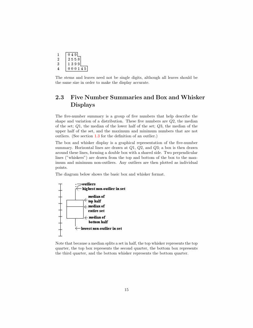
The stems and leaves need not be single digits, although all leaves should bethe same size in order to make the display accurate.
2.3 Five Number Summaries and Box and WhiskerDisplays
The five-number summary is a group of five numbers that help describe theshape and variation of a distribution. These five numbers are Q2, the medianof the set; Q1, the median of the lower half of the set; Q3, the median of theupper half of the set, and the maximum and minimum numbers that are notoutliers. (See section 1.3 for the definition of an outlier.)
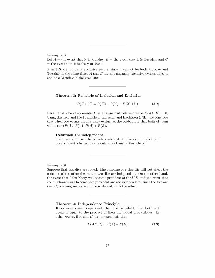
The box and whisker display is a graphical representation of the five-numbersummary. Horizontal lines are drawn at Q1, Q2, and Q3; a box is then drawnaround these lines, forming a double box with a shared side. Two perpendicularlines (”whiskers”) are drawn from the top and bottom of the box to the max-imum and minimum non-outliers. Any outliers are then plotted as individualpoints.
The diagram below shows the basic box and whisker format.
Note that because a median splits a set in half, the top whisker represents the topquarter, the top box represents the second quarter, the bottom box representsthe third quarter, and the bottom whisker represents the bottom quarter.
15

Chapter 3
Probability
3.1 Introduction
Definition 12: probability.The probability of a specific event is a mathematical statement aboutthe likelihood that it will occur. All probabilities are numbers be-tween 0 and 1, inclusive; a probability of 0 means that the event willnever occur, and a probability of 1 means that the event will alwaysoccur.
The sum of the probabilities of all possible outcomes of any event is 1. (This isbecause something will happen, so the probability of some outcome occurringis 1.)
Definition 13: complimentary event.With respect to an event E, the complimentary event, denoted E′,is the event that E does not occur. For example, consider the eventthat it will rain tomorrow. The compliment of this event is the eventthat it will not rain tomorrow.
Since an event must either occur or not occur, from above, it mustbe the case that
P (E) + P (E′) = 1 (3.1)
Definition 14: mutually exclusive.Two or more events are mutually exclusive if they cannot occursimultaneously.
Two events A and B are mutually exclusive if A ∪ B = 0 - that is,if they have no members in common.
16
——————————–
Example 8:Let A = the event that it is Monday, B = the event that it is Tuesday, and C= the event that it is the year 2004.
A and B are mutually exclusive events, since it cannot be both Monday andTuesday at the same time. A and C are not mutually exclusive events, since itcan be a Monday in the year 2004.
——————————–
Theorem 3: Principle of Inclusion and Exclusion
P (X ∪ Y ) = P (X) + P (Y )− P (X ∩ Y ) (3.2)
Recall that when two events A and B are mutually exclusive P (A ∩ B) = 0.Using this fact and the Principle of Inclusion and Exclusion (PIE), we concludethat when two events are mutually exclusive, the probability that both of themwill occur (P (A ∪B)) is P (A) + P (B).
Definition 15: independent.Two events are said to be independent if the chance that each oneoccurs is not affected by the outcome of any of the others.
——————————–
Example 9:Suppose that two dice are rolled. The outcome of either die will not affect theoutcome of the other die, so the two dice are independent. On the other hand,the event that John Kerry will become president of the U.S. and the event thatJohn Edwards will become vice president are not independent, since the two are(were?) running mates, so if one is elected, so is the other.
——————————–
Theorem 4: Independence PrincipleIf two events are independent, then the probability that both willoccur is equal to the product of their individual probabilities. Inother words, if A and B are independent, then
P (A ∩B) = P (A) + P (B) (3.3)
17

Definition 16: factorial.The factorial of an integer n is defined as the product of all thepositive integers from 1 to n, that is
n! (read “n factorial”) = n · (n− 1) · (n− 2) · · · 3 · 2 · 1 (3.4)
0! is defined to be 1.
Definition 17: combination.A combination is a set of unordered (i.e. order does not matter)items. If we are to choose k distinct objects from a total of n objects,then there are
(nk
)different combinations, where(
n
k
)=
n!k!(n− k)!
(3.5)
Formula 1: Binomial FormulaSuppose that an event occurs with probability p. Then the prob-ability that it will occur exactly x times out of a total of n trialsis (
n
x
)· px(1− p)n−x =
n!x!(n− x)!
· px(1− p)n−x (3.6)
——————————–
Example 10:Derive a formula for calculating P(x) (the probability of x successes out of ntrials, where the probability of each success is p) in terms of x, n, p, and P (x−1).
The probability of x− 1 successes is, using the binomial formula,
P (x− 1) =(
n
x− 1
)· px−1(1− p)n−(x−1)
=n!
(x− 1)!(n− x + 1)!px−1(1− p)n−x+1
The probability of x successes is, again using the binomial formula,
P (x) =(
n
x
)· px(1− p)n−x
=n!
x!(n− x)!· px(1− p)n−x
18
We want to find an expression K such that P (x− 1) ·K = P (x). Thus,
n! · px−1(1− p)n−x+1
(x− 1)!(n− x + 1)!·K =
n! · px(1− p)n−x
x!(n− x)!·
n! · px−1(1− p)n−x(1− p)(x− 1)!(n− x)!(n− x + 1)
·K =n! · p · px−1(1− p)n−x
x(x− 1)!(n− x)!1− p
(n− x + 1)·K =
p
x
K =n− x + 1
x· p
1− p
Hence, the desired formula is
P (x) =n− x + 1
x· p
1− p· P (x− 1) (3.7)
——————————–
3.2 Random Variables
3.2.1 Definition
Definition 18: random variable.A variable that may take on different values depending on the out-come of some event.
——————————–
Example 11:On the AP Statistics exam, 1
5 of the class received an 5, 13 received a 4, 1
6received a 3, 1
20 received a 2, and 13 received an 1. If x represents the score of
a randomly chosen student in the class, then x is a random variable that takesthe values 1, 2, 3, 4, and 5.
——————————–
A random variable may be discrete (it takes on a finite number of values) orcontinuous (it can take on any value in a certain interval, that is, an infinitenumber of values).
Definition 19: probability distribution.A list or formula that gives the probability for each discrete value ofa random variable.
19
3.2.2 Expected Value
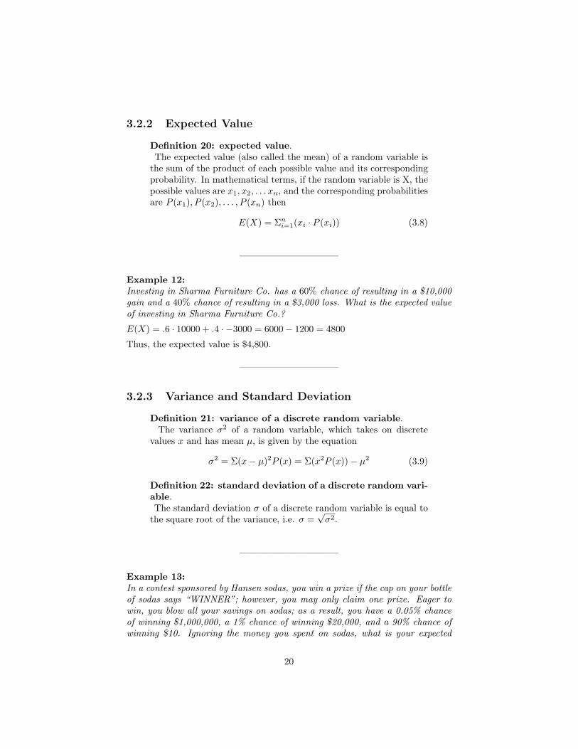
Definition 20: expected value.The expected value (also called the mean) of a random variable is
the sum of the product of each possible value and its correspondingprobability. In mathematical terms, if the random variable is X, thepossible values are x1, x2, . . . xn, and the corresponding probabilitiesare P (x1), P (x2), . . . , P (xn) then
E(X) = Σni=1(xi · P (xi)) (3.8)
——————————–
Example 12:Investing in Sharma Furniture Co. has a 60% chance of resulting in a $10,000gain and a 40% chance of resulting in a $3,000 loss. What is the expected valueof investing in Sharma Furniture Co.?
E(X) = .6 · 10000 + .4 · −3000 = 6000− 1200 = 4800
Thus, the expected value is $4,800.
——————————–
3.2.3 Variance and Standard Deviation
Definition 21: variance of a discrete random variable.The variance σ2 of a random variable, which takes on discrete
values x and has mean µ, is given by the equation
σ2 = Σ(x− µ)2P (x) = Σ(x2P (x))− µ2 (3.9)
Definition 22: standard deviation of a discrete random vari-able.The standard deviation σ of a discrete random variable is equal to
the square root of the variance, i.e. σ =√
σ2.
——————————–
Example 13:In a contest sponsored by Hansen sodas, you win a prize if the cap on your bottleof sodas says “WINNER”; however, you may only claim one prize. Eager towin, you blow all your savings on sodas; as a result, you have a 0.05% chanceof winning $1,000,000, a 1% chance of winning $20,000, and a 90% chance ofwinning $10. Ignoring the money you spent on sodas, what is your expected
20

value and standard deviation?
First, we calculate the mean.
µ = 1000000 · 0.0005 + 0.01 · 20000 + 0.9 · 10 = 500 + 200 + 9 = 709
Now, the variance.
σ2 = 10000002 · 0.0005 + 200002 · 0.01 + 102 · .9− 7092
= 500000000 + 4000000 + 90− 502681= 503497409
Finally, the standard deviation.
σ =√
503497409 ≈ 22438
The standard deviation is over $22,000! Although the expected value looks nice,there’s a good chance that you’ll get a not-so-good amount of money.
——————————–
3.2.4 “Shortcuts” for Binomial Random Variables
The past examples required a fair amount of arithmetic. To save time, thereare simpler ways to find expected values, variances, and standard deviations ofbinomial random variables (that is, random variables with only two outcomes).
Theorem 5: Mean and Standard Deviation of a BinomialIn a situation with two outcomes where the probability of an out-come O is p and there are n trials, the expected number of Os is np.That is,
µ = np (3.10)
Furthermore, the variance σ2 is given by the equation
σ2 = np(1− p) (3.11)
and the standard deviation σ by the equation
σ =√
np(1− p) (3.12)
21

Chapter 4
Probability Distributions
4.1 Binomial Distributions
Previously, we computed the probability that a binomial event (one with twopossible outcomes for each trial) would occur. In the same way, we can computethe probability of every possible combination of outcomes and create a table orhistogram from it.
——————————–
Example 14:On a five-item true or false test, Simon has an 80% chance of choosing the cor-rect answer for any of the questions. Find the complete probability distributionfor the number of correct answers that Simon can get. Then determine the meanand standard deviation of the probability distribution.
P (0) =(
50
)(0.8)0(0.2)5 = 1 · 1 · 0.00032 = 0.00032
P (1) =(
51
)(0.8)1(0.2)4 = 5 · 0.8 · 0.0016 = 0.0064
P (2) =(
52
)(0.8)2(0.2)3 = 10 · 0.64 · 0.008 = 0.0512
P (3) =(
53
)(0.8)3(0.2)2 = 10 · 0.512 · 0.04 = 0.2048
P (4) =(
54
)(0.8)4(0.2)1 = 5 · 0.4096 · 0.2 = 0.4096
P (5) =(
55
)(0.8)5(0.2)0 = 1 · 0.32768 · 1 = 0.32768
22

Note that 0.00032 + 0.0064 + 0.0512 + 0.2048 + 0.4096 + 0.32768 = 1.
The expected value may be calculated in two ways: µ = np = 5 · 0.8 = 4 orµ = 0 · 0.00032 + 1 · 0.0064 + 2 · 0.0512 + 3 · 0.2048 + 4 · 0.4096 + 5 · 0.32768 = 4.In either case, the answer is the same.
The variance is σ2 = np(1−p) = 5·0.8·(1−0.8) = 0.8, so the standard deviationis σ =
√0.8 ≈ 0.894.
——————————–
Binomial distributions are often used in quality control systems, where a smallnumber of samples are tested out of a shipment, and the shipment is onlyaccepted if the number of defects found among the sampled units falls below aspecified number. In order to analyze whether a sampling plan effectively screensout shipments containing a great number of defects and accepts shipments withvery few defects, one must calculate the probability that a shipment will beaccepted given various defect levels.
——————————–
Example 15:A sampling plan calls for twenty units out of a shipment to be sampled. Theshipment will be accepted if and only if the number of defective units is less thanor equal to one. What is the probability that a shipment with defect level n willbe accepted for n = 0.05, 0.10, 0.15, 0.20, 0.25, 0.30?
P (acceptance) = P (0 defective units) + P (1 defective unit)
=(
2020
)n0 · (1− n)20 +
(2019
)n1 · (1− n)19
= (1− n)20 + 20 · (1− n)19 · n
If n = 0.05, P (acceptance) = (0.95)20 + 20(0.95)19(0.05)1 = 0.736If n = 0.10, P (acceptance) = (0.90)20 + 20(0.90)19(0.10)1 = 0.392If n = 0.15, P (acceptance) = (0.85)20 + 20(0.85)19(0.15)1 = 0.176If n = 0.20, P (acceptance) = (0.80)20 + 20(0.80)19(0.20)1 = 0.069If n = 0.25, P (acceptance) = (0.75)20 + 20(0.75)19(0.25)1 = 0.024If n = 0.30, P (acceptance) = (0.70)20 + 20(0.70)19(0.30)1 = 0.008
——————————–
23
4.2 Poisson Distributions
4.2.1 Definition
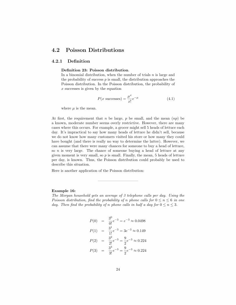
Definition 23: Poisson distribution.In a binomial distribution, when the number of trials n is large andthe probability of success p is small, the distribution approaches thePoisson distribution. In the Poisson distribution, the probability ofx successes is given by the equation
P (x successes) =µx
x!e−µ (4.1)
where µ is the mean.
At first, the requirement that n be large, p be small, and the mean (np) bea known, moderate number seems overly restrictive. However, there are manycases where this occurs. For example, a grocer might sell 5 heads of lettuce eachday. It’s impractical to say how many heads of lettuce he didn’t sell, becausewe do not know how many customers visited his store or how many they couldhave bought (and there is really no way to determine the latter). However, wecan assume that there were many chances for someone to buy a head of lettuce,so n is very large. The chance of someone buying a head of lettuce at anygiven moment is very small, so p is small. Finally, the mean, 5 heads of lettuceper day, is known. Thus, the Poisson distribution could probably be used todescribe this situation.
Here is another application of the Poisson distribution:
——————————–
Example 16:The Morgan household gets an average of 3 telephone calls per day. Using thePoisson distribution, find the probability of n phone calls for 0 ≤ n ≤ 6 in oneday. Then find the probability of n phone calls in half a day for 0 ≤ n ≤ 3.
P (0) =30
0!e−3 = e−3 ≈ 0.0498
P (1) =31
1!e−3 = 3e−3 ≈ 0.149
P (2) =32
2!e−3 =
92e−3 ≈ 0.224
P (3) =33
3!e−3 =
92e−3 ≈ 0.224
24
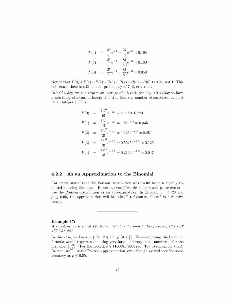
P (4) =34
4!e−3 =
278
e−3 ≈ 0.168
P (5) =35
5!e−3 =
8140
e−3 ≈ 0.100
P (6) =36
6!e−3 =
8180
e−3 ≈ 0.050
Notice that P (0)+P (1)+P (2)+P (3)+P (4)+P (5)+P (6) ≈ 0.96, not 1. Thisis because there is still a small probability of 7, 8, etc. calls.
In half a day, we can expect an average of 1.5 calls per day. (It’s okay to havea non-integral mean, although it is true that the number of successes, x, mustbe an integer.) Thus,
P (0) =1.50
0!e−1.5 = e−1.5 ≈ 0.223
P (1) =1.51
1!e−1.5 = 1.5e−1.5 ≈ 0.335
P (2) =1.52
2!e−1.5 = 1.125e−1.5 ≈ 0.251
P (3) =1.53
3!e−1.5 = 0.5625e−1.5 ≈ 0.126
P (4) =1.54
4!e−1.5 = 0.2109e−1.5 ≈ 0.047
——————————–
4.2.2 As an Approximation to the Binomial
Earlier we stated that the Poisson distribution was useful because it only re-quired knowing the mean. However, even if we do know n and p, we can stilluse the Poisson distribution as an approximation. In general, if n ≥ 20 andp ≤ 0.05, the approximation will be “close” (of course, “close” is a relativeterm).
——————————–
Example 17:A standard die is rolled 120 times. What is the probability of exactly 10 sixes?15? 20? 25?
In this case, we know n (it’s 120) and p (it’s 16 ). However, using the binomial
formula would require calculating very large and very small numbers - for thefirst one,
(12010
). (For the record, it’s 116068178638776. Try to remember that!)
Instead, we’ll use the Poisson approximation, even though we will sacrifice someaccuracy as p 6≤ 0.05.
25

The expected value is np = 120 · 16 = 20. So
P (10) =2010
10!e−20 ≈ 0.0058
P (15) =2015
15!e−20 ≈ 0.0516
P (20) =2020
20!e−20 ≈ 0.0888
P (25) =2025
25!e−20 ≈ 0.0446
The actual values are
P (10) =(
12010
) (16
)10 (56
)110
≈ 0.0037
P (15) =(
12015
) (16
)15 (56
)105
≈ 0.0488
P (20) =(
12020
) (16
)20 (56
)100
≈ 0.0973
P (25) =(
12025
) (16
)25 (56
)95
≈ 0.0441
——————————–
4.3 Normal Distributions
4.3.1 Definition and Properties
The normal curve is a bell-shaped, symmetrical graph with an infinitely longbase. The mean, median, and mode are all located at the center.
A value is said to be normally distributed if its histogram is the shape of thenormal curve. The probability that a normally distributed value will fall betweenthe mean and some z-score z is the area under the curve from 0 to z:
26

4.3.2 Table of Normal Curve Areas
The area from the mean to z-score z is given in the table below:
z 0 1 2 3 4 5 6 7 8 90.0 .0000 .0040 .0080 .0120 .0160 .0199 .0239 .0279 .0319 .03590.1 .0398 .0438 .0478 .0517 .0557 .0596 .0636 .0675 .0714 .07530.2 .0793 .0832 .0871 .0910 .0948 .0987 .1026 .1064 .1103 .11410.3 .1179 .1217 .1255 .1293 .1331 .1368 .1406 .1443 .1480 .15170.4 .1554 .1591 .1628 .1664 .1700 .1736 .1772 .1808 .1844 .18790.5 .1915 .1950 .1985 .2019 .2054 .2088 .2123 .2157 .2190 .22240.6 .2257 .2291 .2324 .2357 .2389 .2422 .2454 .2486 .2517 .25490.7 .2580 .2611 .2642 .2673 .2704 .2734 .2764 .2794 .2823 .28520.8 .2881 .2910 .2939 .2967 .2995 .3023 .3051 .3078 .3106 .31330.9 .3159 .3186 .3212 .3238 .3264 .3289 .3315 .3340 .3365 .33891.0 .3413 .3438 .3461 .3485 .3508 .3531 .3554 .3577 .3599 .36211.1 .3643 .3665 .3686 .3708 .3729 .3749 .3770 .3790 .3810 .38301.2 .3849 .3869 .3888 .3907 .3925 .3944 .3962 .3980 .3997 .40151.3 .4032 .4049 .4066 .4082 .4099 .4115 .4131 .4147 .4162 .41771.4 .4192 .4207 .4222 .4236 .4251 .4265 .4279 .4292 .4306 .43191.5 .4332 .4345 .4357 .4370 .4382 .4394 .4406 .4418 .4429 .44411.6 .4452 .4463 .4474 .4484 .4495 .4505 .4515 .4525 .4535 .45451.7 .4554 .4564 .4573 .4582 .4591 .4599 .4608 .4616 .4625 .46331.8 .4641 .4649 .4656 .4664 .4671 .4678 .4686 .4693 .4699 .47061.9 .4713 .4719 .4726 .4732 .4738 .4744 .4750 .4756 .4761 .47672.0 .4772 .4778 .4783 .4788 .4793 .4798 .4803 .4808 .4812 .48172.1 .4821 .4826 .4830 .4834 .4838 .4842 .4846 .4850 .4854 .48572.2 .4861 .4864 .4868 .4871 .4875 .4878 .4881 .4884 .4887 .48902.3 .4893 .4896 .4898 .4901 .4904 .4906 .4909 .4911 .4913 .49162.4 .4918 .4920 .4922 .4925 .4927 .4929 .4931 .4932 .4934 .49362.5 .4938 .4940 .4941 .4943 .4945 .4946 .4948 .4949 .4951 .49522.6 .4953 .4955 .4956 .4957 .4958 .4960 .4961 .4962 .4963 .49642.7 .4965 .4966 .4967 .4968 .4969 .4970 .4971 .4972 .4973 .49742.8 .4974 .4975 .4976 .4977 .4977 .4978 .4979 .4979 .4980 .49812.9 .4981 .4982 .4982 .4983 .4984 .4984 .4985 .4985 .4986 .49863.0 .4987 .4987 .4987 .4988 .4988 .4989 .4989 .4989 .4990 .4990
27

——————————–
Example 18:The price of a gallon of gasoline at the gasoline stations in Nevada is normallydistributed with a mean of $2.00 and a standard deviation of $0.50.
What is the probability that at a randomly chosen gasoline station in Nevada,the price of gasoline will be between $2.00 and $2.75?
The z-score of $2.00 is 0, and the z-score of $2.75 is$2.75− $2.00
$0.50= 1.5. Ac-
cording to the table above, the area between 0 and 1.5 is 0.4332 of the totalarea, so the probability is 0.4332.
What is the probability that at a randomly chosen gasoline station in Nevada,the price of gasoline will be between $1.25 and $2.00?
The z-score of $1.25 is$1.75− $2.00
$0.50= −1.5, and the z-score of $2.00 is 0. But
since the normal curve is symmetric, the area between −1.5 and 0 is the sameas the area between 0 and 1.5, which is, as before, 0.4332 of the total area. Thusthe probability is also 0.4332.
What percent of the gasoline stations have prices between $1.13 and $3.20?
The z-score of $1.13 is$1.13− $2.00
$0.50= −1.74, and the z-score of $3.20 is
$3.20− $2.00$0.50
= 2.40. The area between -1.74 and 2.40 is equal to the area be-
tween -1.74 and 0 plus the area between 0 and 2.40, which is 0.4591 + 0.4918 =0.9509 ≈ 95.1%.
What is the probability that a randomly chosen gas station will have pricesgreater than $3.15 per gallon?
The z score of $3.15 is$3.15− $2.00
$0.50= 2.30. We want to find the probability
P (greater than 2.30). But how can we do this? 0 isn’t greater than 2.30, so itappears that we can’t use the probabilities from the above table.
Appearances can be deceiving. First, note that, in terms of z-scores, P (between0 and 2.30) + P (greater than 2.30) = P (greater than 0). Thus, P (greater than2.30) = P (greater than 0) - P (between 0 and 2.30).
The probability that the gas station will be between 0 and 2.30 is 0.4893, and theprobability that the gas station will be greater than 0 is 0.5, so the probabilitythat the gas station will be greater than 2.30 is 0.5− 0.4893 = 0.0107
——————————–
28

4.3.3 Working Backwards
In the previous examples, we found percentages and probabilities given rawdata. We can work in the reverse direction just as easily. For example, supposewe wanted to know what z-score 90% of a normal distribution was greater than.Thus, we want 10% to be less than some score z, or 40% to be between z and 0.Looking at the table, we see that a z-score of 1.28 corresponds to 0.3997, whichis very close to 0.4, so z is -1.28. Thus, 90% of the normal distribution has a zscore greater than -1.28. Working similarly, we obtain the following facts:
• 90% of the normal distribution is between z-scores of -1.645 and 1.645.
• 95% of the normal distribution is between z-scores of -1.96 and 1.96.
• 99% of the normal distribution is between z-scores of -2.58 and 2.58.
• 90% of the normal distribution is less than the z-score of 1.28, and 90%of the normal distribution is greater than the z-score of -1.28.
• 95% of the normal distribution is less than the z-score of 1.645, and 95%of the normal distribution is greater than the z-score of -1.645.
• 99% of the normal distribution is less than the z-score of 2.33, and 99%of the normal distribution is greater than the z-score of -2.33.
• 68.26% of the normal distribution is between z-scores of -1 and 1.
• 95.44% of the normal distribution is between z-scores of -2 and 2.
• 99.74% of the normal distribution is between z-scores of -3 and 3.
If we do not know the mean or standard deviation, we can also work backwardto find it.
——————————–
Example 19:A normal distribution has a mean of 36, and 19% of the values are above 50.What is the standard deviation?
Since 0.19 of the distribution is above 50, 0.31 of the distribution is between 36(the mean) and 50. Looking at the table of normal curve areas, 0.31 correspondsto a z-score of 0.88, so 50 is 0.88 standard deviations above the mean. Thus,50 = 36 + 0.88σ, or 0.88σ = 14. Therefore σ = 15.91.
——————————–
29

4.3.4 As an Approximation to the Binomial
The normal may also be viewed as a limiting case to the binomial, so we mayuse it to approximate the value of a binomial for large n. However, becausethe binomial only takes values at integers, whereas the normal is a continuouscurve, we will represent an integer value with a unit-long interval centered atthat integer. (For example, 4 would be represented by the interval from 3.5 to4.5.)
——————————–
Example 20:Shaquille O’Neal averages 0.627 on free throws. What is the probability that outof 100 attempts, he will have made exactly 70 of them?
First, we calculate µ and σ. µ = np = 100 ·0.627 = 62.7 and σ =√
np(1− p) =√62.7 · 0.373 ≈ 4.84.
Then, recalling that we will represent 70 with the interval from 69.5 to 70.5, wecalculate some z-scores. The z-score of 69.5 is 69.5−62.7
4.84 = 1.405, and the z-scoreof 70.5 is 70.5−62.7
4.84 = 1.612. The area from 0 to 1.612 is 0.4463 and the areafrom 0 to 1.405 is 0.4207, so the final probability is 0.4463− 0.4207 = 0.0256.
——————————–
In general, the normal is considered a “good” approximation when both np andn(1− p) are greater than 5.
30

Chapter 5
The Population Mean
Oftentimes it is impossible or impractical to survey an entire population. Forexample, a manufacturer cannot test every battery, or it wouldn’t have any tosell. Instead, a sample must be taken and tested. This gives birth to manyquestions: what size sample should be taken to be accurate? How accurate isaccurate? How can we ensure that a sample is representative of a population?What conclusions can we draw about the population using the sample? And soon. In this section, we’ll discuss samples and answer some of these questions.
5.1 The Distribution of Sample Means
As mentioned before, we want to estimate a population’s mean by surveyinga small sample. If the sample is very small, say it contains one member, thenthe mean of the sample is unlikely to be a good estimate of the population. Aswe increase the number of members, the estimate will improve. Thus, biggersample size generally results in a sample mean that is closer to the populationmean.
Similarly, if we survey individual members of a population, their values areunlikely to be normally distributed - individuals can easily throw things off withwidely varying values. However, if we take several samples, then the samplemeans are likely to be normally distributed, because the individuals in eachsample will generally balance each other out.
Theorem 6: Central Limit TheoremStart with a population with a given mean µ and standard deviationσ. Take samples of size n, where n is a sufficiently large (generallyat least 30) number, and compute the mean of each sample.
• The set of all sample means will be approximately normallydistributed.
31

• The mean of the set of samples will equal µ, the mean of thepopulation.
• The standard deviation, σx, of the set of sample means will beapproximately
σ√n
.
——————————–
Example 21:Foodland shoppers have a mean $60 grocery bill with a standard deviation of$40. What is the probability that a sample of 100 Foodland shoppers will havea mean grocery bill of over $70?
Since the sample size is greater than 30, we can apply the Central Limit Theo-rem. By this theorem, the set of sample means of size 100 has mean $60 and stan-
dard deviation$40√100
= $4. Thus, $70 represents a z-score of$70− $60
$4= 2.5.
Since the set of sample means of size 100 is normally distributed, we can com-pare a z-score of 2.5 to the table of normal curve areas. The area between z = 0and z = 2.5 is 0.4938, so the probability is 0.5 - 0.4938 = 0.0062.
——————————–
5.2 Confidence Interval Estimatess
We can find the probability that a sample lies within a certain interval of thepopulation mean by using the central limit theorem and the table or normalcurve areas. But this is the same as the probability that the population meanlies within a certain interval of a sample. Thus, we can determine how con-fident we are that the population mean lies within a certain intervalof a sample mean.
——————————–
Example 22:At a factory, batteries are produced with a standard deviation of 2.4 months.In a sample of 64 batteries, the mean life expectancy is 12.35. Find a 95%confidence interval estimate for the life expectancy of all batteries produced atthe plant.
Since the sample has n larger than 30, the central limit theorem applies. Letthe standard deviation of the set of sample means of size 64 be σx. Then by thecentral limit theorem, 2.4 =
σx√64
, so σx = 0.3 months.
32

Looking at the table of normal curve areas (or referring to section 4.3.3), 95%of the normal curve area is between the z-scores of -1.96 and 1.96. Since thestandard deviation is 0.3, a z-score of −1.96 represents a raw score of -0.588months, and a z-score of 1.96 represents a raw score of 0.588 months. So we have95% confidence that the life expectancy will be between 12.35− 0.588 = 11.762months and 12.35 + 0.588 = 12.938 months.
——————————–
If we do not know σ (the standard deviation of the entire population), we uses (the standard deviation of the sample) as an estimate for σ. Recall that s isdefined as
s =
√Σ(x− x)2
n− 1=
Σx2 − (Σx)2
nn− 1
(5.1)
where x takes on each individual value, x is the sample mean, and n is thesample size.
5.3 Choosing a Sample Size
Note that as the degree of confidence increases, the interval must become larger;conversely, as the degree of confidence decreases the interval becomes moreprecise. This is true in general; if we want to be more sure that we are right, wesacrifice precision, and if we want to be closer to the actual value, we are lesslikely to be right.
There is a way to improve both the degree of confidence and the precision ofthe interval: by increasing the sample size. So it seems like greater sample sizeis always desirable; however, in the real world, increasing the sample size coststime and money.
Generally, we will be asked to find the minimum sample size that will result ina desired confidence level and range.
——————————–
Example 23:A machine fills plastic bottles with Mountain Dew brand soda with a standarddeviation of 0.04 L. How many filled bottles should be tested to determine themean volume of soda to an accuracy of 0.01 L with 95% confidence?
Let σx be the standard deviation of the sample. Since σx =σ√n
, we have
σx =0.04L√
n. Also, since 95% confidence corresponds to z-scores from -1.96 to
33

1.96 on the normal curve, we have 0.01L = σx · 1.96. Substituting, we obtain
0.01L =0.04L√
n· 1.96
√n =
0.04L
0.01L· 1.96
√n = 7.84n = 61.4656
So at least 62 bottles should be tested.
——————————–
5.4 The Hypothesis Test
Oftentimes we want to determine whether a claim is true or false. Such a claimis called a hypothesis.
Definition 24: null hypothesis.A specific hypothesis to be tested in an experiment. The null hy-pothesis is usually labeled H0.
Definition 25: alternative hypothesis.A hypothesis that is different from the null hypothesis, which we usu-ally want to show is true (thereby showing that the null hypothesisis false). The alternative hypothesis is usually labeled Ha.
If the alternative involves showing that some value is greater thanor less than a number, there is some value c that separates the nullhypothesis rejection region from the fail to reject region. This valueis known as the critical value.
The null hypothesis is tested through the following procedure:
1. Determine the null hypothesis and an alternative hypothesis.
2. Pick an appropriate sample.
3. Use measurements from the sample to determine the likelihood of the nullhypothesis.
Definition 26: Type I error.If the null hypothesis is true but the sample mean is such that thenull hypothesis is rejected, a Type I error occurs. The probabilitythat such an error will occur is the α risk.
34

Definition 27: Type II error.If the null hypothesis is false but the sample mean is such that thenull hypothesis cannot be rejected, a Type II error occurs. Theprobability that such an error will occur is called the β risk.
——————————–
Example 24:A government report claims that the average temperature on the planet Venusis at least 300◦ C. You don’t believe this - you think the average temperaturemust be lower - so you carry out an experiment during which you will measurethe temperature on Venus at 100 random times, then compute the mean of themeasured temperatures. If the mean temperature is over 20◦ C less than thereport’s claim, then you will declare the report’s claim false.
Thus, the null hypothesis is H0 : T = 300 and the alterative hypothesis isHa : T < 300. The value c = 280 separates the rejection region from the failto reject region; that is, if T < 280, the null hypothesis will be rejected, and ifT ≥ 280, then the null hypothesis will not be rejected.
Suppose that the actual temperature on Venus is indeed 300◦ C (or greater), asthe report stated. If the sample mean has T ≥ 280, then the null hypothesis willcorrectly be accepted. If the sample mean has T < 280 then the null hypothesiswill incorrectly be rejected; this is a Type I error. On the other hand, if theactual temperature on Venus is less than 300◦ C, but the sample mean hasT ≥ 280, then the null hypothesis will incorrectly be accepted; this is a Type IIerror. If the sample mean has T < 280, then the null hypothesis will correctlybe rejected.
——————————–
5.5 More on Errors
5.5.1 Type I Errors and α-Risks
We can calculate the α-risk (that is, the probability of a Type I error) by drawingthe normal curve assuming that the null hypothesis is true, then determiningthe area of the region which corresponds to the probability that the test resultsin the rejection of the null hypothesis.
——————————–
Example 25:A school district claims that an average of $7,650 is being spent on each child
35

each year. The state budget director, suspicious that some of the money allocatedto the school district is not being spent on the schools, suspects that the figureis actually smaller. He will measure the exact amount of money spent on 36students and wil reject the school district’s claim if the average amount spent isless than $7,200. If the standard deviation in amount spent per pupil is $1,200,what is the α-risk?
The α-risk is the probability that a Type I error, where the null hypothesisis true but is rejected, so to calculate it, we will look at the case where thenull hypothesis is true, i.e. µ = 7650. Since the sample size is over 30, weapply the central limit theorem. The standard deviation of a sample of size
36 is1200√
36=
12006
= 200. The mean of the sample means is equal to the
actual mean, which is 7650. Thus, the z-score that corresponds to 7200 is7200−7650
200 = − 450200 = −2.25. The area under the normal curve from −2.25 to 0 is
0.4878, so the area of the z-scores less than −2.25 is −0.0122. Thus, the α-riskis −0.0122.
——————————–
In the previous example, we calculated the α-risk given the critical value(s).However, it is often more useful to determine critical values given an acceptableα-risk level (called the significance level of the test).
After we determine the critical values, it is a simple task to determine whetherthe sample mean (or, potentially, some other sample statistic) falls in the re-jection range or the fail to reject range. This is how we draw conclusions: byshowing that the null hypothesis is improbable.
Definition 28: p-value.The p-value of a test is the smallest value of α for which the nullhypothesis would be rejected. An alternative definition is the prob-ability of obtaining the experimental result if the null hypothesis istrue. Smaller p-values mean more significant differences between thenull hypothesis and the sample result.
——————————–
Example 26:A drug company claims that their medication will render a patient unconsciousin an average of 5.76 minutes. A researcher decides to test this claim with 300patients. He obtains the following data: Σx = 2789 and Σ(x − x)2 = 3128.Should the drug company’s claim be rejected at a level of 10% significance?
36

We calculate the sample mean and sample standard deviation as follows:
x =Σx
n=
2789300
≈ 9.297
s =
√Σ(x− x)2
n− 1=
√3128299
≈ 3.234
σx ≈ s√n
=3.234300
≈ 0.187
A level of 10% significance means that α = 0.1. Recall that a Type I error isone in which the null hypothesis is true but the data causes it to be rejected.So for our purposes, we will consider the case where the null hypothesis is true,and the time it takes to render a patient unconscious is 5.76 minutes. A TypeI error will occur either if the sample mean is above or below 5.76, so we mustconsider both possibilites - this is called a two-sided, or two-tailed, test - thebottom 0.05 and the top 0.05.
According to the table of normal curve areas, between −1.645 and 0, the areaunder the normal curve is 0.45, so if the z-score is less than −1.645, the area is0.05, as desired. Similarly, if the z-score is greater than 1.645, the area is also0.05. So a Type I error will occur if the z-score is less than −1.645 or greaterthan 1.645. We must now convert to raw score. Since the mean of sample meansis 5.76 and the standard deviation of sample means is 0.187, a z-score of −1.645corresponds to a raw score of 5.76+0.187(−1.645) = 5.45, and a z-score of 1.645corresponds to a raw score of 5.76 + 0.187(1.645) = 6.07. So the critical valuesof the experiment should be 5.45 and 6.07. Since 9.297 > 6.06, the claim shouldbe rejected.
——————————–
5.5.2 Type II Errors and β-Risks
The β-risk (that is, the probability of failing to reject the null hypothesis) differsdepending on the actual population statistic. We calculate it in a way similarto the calculation of the α-risk - by considering a possible actual value forthe population, using this value as the center of the normal distribution, andcalculating the area beyond the critical point that corresponds to the fail toreject zone.
——————————–
Example 27:A poll claims that children spend an average of 203 minutes per day watchingtelevision. A researcher believes this is too high and conducts a study of 144patients. The sample standard deviation is 120 minutes. He will reject the
37

claim if the sample mean is under 180 minutes per day. What is the probabilityof a Type II error if the actual average is 210? 175? 170?
The standard deviation of the sample means is
σx ≈s√n
=120√144
=12012
= 10
The null hypothesis will not be rejected if the sample mean is above 180.Thus, we look for the probability of the sample mean being above 180 todetermine the β-risk. If the actual average is 210 minutes, then the samplemeans will be normally distributed about 210, so the z-score of the criticalvalue, 180, is 180−210
10 = −3, which corresponds to a probability of 0.4987.Thus, the probability of the sample mean being less than 180 (i.e. rejection) is0.5−0.4987, and the probability of this not being the case (i.e. failure to reject)is 0.5 + 0.4987 = 0.9987. This is the β-risk.
If the actual average is 175 minutes, then the sample means will be normallydistributed about 175, so the z-score of the critical value, 180, is 180−175
10 = 0.5,which corresponds to a probability of 0.1915. Thus, the probability of the samplemean being greater than 180 is 0.5− 0.1915 = .3085.
If the actual average is 170 minutes, then the sample means will be normallydistributed about 170, so the z-score of the critical value, 170, is 180−170
10 = 1,which corresponds to a probability of 0.3413. This is the probability that thesample mean is between 170 and 180. Thus, the probability of the sample meanbeing greater than 180 is 0.5− 0.3413 = .1587.
——————————–
In the past example, we were given a critical value. Instead, we may be given anacceptable α-risk, from which we can calculate the critical value. We can thenuse the critical value to calculate β-risks for possible actual values. In general,we can use the following pathway:
acceptable α-risk (significance level) ←→ critical value(s) −→ β-risk
5.6 Comparing Two Means
5.6.1 Confidence Interval Estimates
We can compare the means of two populations by comparing the means of theirsamples. More specifically, we can compute a confidence interval estimate forthe difference between the two means (i.e. µ1−µ2). We do this using the samemethod that we did for finding a confidence interval estimate for one value,
38

except that we use
µ = µ1 − µ2 (5.2)
σx =
√σ2
1
n1+
σ22
n2(5.3)
x = x1 − x2 (5.4)
39

Index
alternative hypothesis, 31
bar graph, 9bimodal, 3binomial distribution, 19
in quality control systems, 20Binomial Formula, 15binomial random variable, 18box and whisker display, 12
Central Limit Theorem, 28Chebyshev’s Theorem, 7combination, 15complimentary event, 13confidence interval
estimate of, 29
data typesdiscrete, 2measured, 2numerical, 2
definitionsalternative hypothesis, 31combination, 15complimentary event, 13expected value, 17factorial, 15histogram, 9independent, 14mean, 3median, 3mode, 3mutually exclusive, 13null hypothesis, 31p-value, 33percentile ranking, 6Poisson distribution, 21
probability, 13probability distribution, 16random variable, 16range, 4relative variability, 5simple ranking, 6standard deviation, 4Type I error, 31Type II error, 32variance, 4z-score, 6
descriptive statistics, 2
empirical rule, 7examples
binomial distribution, 19, 20binomial formula, 15calculating an alpha risk, 32calculating beta-risk, 34calculating modes, 3central limit theorem, 29Chebyshev’s Theorem, 7choosing a sample size, 30confidence interval estimates, 29constructing a histogram from
z-scores, 11determining relative frequency
from a histogram, 10determining statistical significance,
33expected value, 17independent and non-independent
events, 14mutually exclusive events, 13normal as a binomial approxi-
mation, 26normal distribution, 24, 26
40
Poisson distribution, 22Poisson distributions, 21random variables, 16simple, percentile, and z-score
ranking, 6standard deviation of a discrete
random variable, 17stem and leaf display, 11testing a hypothesis and error
types, 32z-scores, 7
expected value, 17
factorial, 15formulae
Binomial Formula, 15
histogram, 9, 10and relative frequencies, 10as compared to bar graph, 9representation of mean, median,
and mode, 10
Independence Principle, 14independent, 14inferential statistics, 2interquartile range, 4
mean, 3, 10arithmetic, 3expected value, 17on a histogram, 10properties of, 4trimmed mean, 4
Mean and Standard Deviation of aBinomial, 18
median, 3, 10in a box and whisker display, 12on a histogram, 10
mode, 3, 10on a histogram, 10
mutually exclusive, 13
normal curve, 23area of, 23
null hypothesis, 31
outlier, 4
p-value, 33percentile ranking, 6Poisson distribution, 21
as an approximation to the bi-nomial, 22
Principle of Inclusion and Exclusion,14
probability, 13probability distribution, 16
random variable, 16standard deviation of, 17variance of, 17
range, 4interquartile range, 4
relative frequency, 9relative variability, 5
sample size, 30simple ranking, 6skewed to the left, 10skewed to the right, 10standard deviation, 4
approximation of, 7of a discrete random variable,
17of a sample, 30
theoremsCentral Limit Theorem, 28Chebyshev’s Theorem, 7empirical rule, 7Independence Principle, 14Mean and Standard Deviation
of a Binomial, 18Principle of Inclusion and Ex-
clusion, 14trimmed mean, 4Type I error, 31Type II error, 32
variance, 4of a discrete random variable,
17of population, 4
41

of sample, 4
z-score, 6
42