an introduction to the finite element method (fem) for...
TRANSCRIPT

An Introduction to theFinite Element Method (FEM)
for Differential Equations
Mohammad Asadzadeh
January 12, 2016


Contents
0 Introduction 70.1 Preliminaries . . . . . . . . . . . . . . . . . . . . . . . . . . . 80.2 Trinities . . . . . . . . . . . . . . . . . . . . . . . . . . . . . . 9
1 Partial Differential Equations 171.1 Differential operators, superposition . . . . . . . . . . . . . . . 19
1.1.1 Exercises . . . . . . . . . . . . . . . . . . . . . . . . . . 221.2 Some equations of mathematical physics . . . . . . . . . . . . 23
1.2.1 Exercises . . . . . . . . . . . . . . . . . . . . . . . . . . 33
2 Polynomial Approximation in 1d 352.1 Overture . . . . . . . . . . . . . . . . . . . . . . . . . . . . . . 352.2 Galerkin finite element method for (2.1.1) . . . . . . . . . . . 462.3 A Galerkin method for (BVP) . . . . . . . . . . . . . . . . . 502.4 Exercises . . . . . . . . . . . . . . . . . . . . . . . . . . . . . . 60
3 Interpolation, Numerical Integration in 1d 633.1 Preliminaries . . . . . . . . . . . . . . . . . . . . . . . . . . . 633.2 Lagrange interpolation . . . . . . . . . . . . . . . . . . . . . . 713.3 Numerical integration, Quadrature rule . . . . . . . . . . . . . 75
3.3.1 Composite rules for uniform partitions . . . . . . . . . 783.3.2 Gauss quadrature rule . . . . . . . . . . . . . . . . . . 82
3.4 Exercises . . . . . . . . . . . . . . . . . . . . . . . . . . . . . . 86
4 Linear Systems of Equations 914.1 Direct methods . . . . . . . . . . . . . . . . . . . . . . . . . . 924.2 Iterative methods . . . . . . . . . . . . . . . . . . . . . . . . . 1004.3 Exercises . . . . . . . . . . . . . . . . . . . . . . . . . . . . . . 109
3

4 CONTENTS
5 Two-point boundary value problems 113
5.1 A Dirichlet problem . . . . . . . . . . . . . . . . . . . . . . . 113
5.2 A mixed Boundary Value Problem . . . . . . . . . . . . . . . 118
5.3 The finite element method (FEM) . . . . . . . . . . . . . . . . 121
5.4 Error estimates in the energy norm . . . . . . . . . . . . . . . 122
5.5 FEM for convection–diffusion–absorption BVPs . . . . . . . . 128
5.6 Exercises . . . . . . . . . . . . . . . . . . . . . . . . . . . . . . 137
6 Scalar Initial Value Problems 145
6.1 Solution formula and stability . . . . . . . . . . . . . . . . . . 146
6.2 Galerkin finite element methods for IVP . . . . . . . . . . . . 147
6.2.1 The continuous Galerkin method . . . . . . . . . . . . 148
6.2.2 The discontinuous Galerkin method . . . . . . . . . . . 151
6.3 A posteriori error estimates . . . . . . . . . . . . . . . . . . . 153
6.3.1 A posteriori error estimate for cG(1) . . . . . . . . . . 153
6.3.2 A posteriori error estimate for dG(0) . . . . . . . . . . 160
6.3.3 Adaptivity for dG(0) . . . . . . . . . . . . . . . . . . . 162
6.4 A priori error analysis . . . . . . . . . . . . . . . . . . . . . . 163
6.4.1 A priori error estimates for the dG(0) method . . . . . 163
6.5 The parabolic case (a(t) ≥ 0) . . . . . . . . . . . . . . . . . . 167
6.5.1 Some examples of error estimates . . . . . . . . . . . . 171
6.6 Exercises . . . . . . . . . . . . . . . . . . . . . . . . . . . . . . 174
7 Initial Boundary Value Problems in 1d 177
7.1 Heat equation in 1d . . . . . . . . . . . . . . . . . . . . . . . . 177
7.1.1 Stability estimates . . . . . . . . . . . . . . . . . . . . 179
7.1.2 FEM for the heat equation . . . . . . . . . . . . . . . . 185
7.1.3 Error analysis . . . . . . . . . . . . . . . . . . . . . . . 188
7.1.4 Exercises . . . . . . . . . . . . . . . . . . . . . . . . . . 196
7.2 The wave equation in 1d . . . . . . . . . . . . . . . . . . . . . 198
7.2.1 Wave equation as a system of hyperbolic PDEs . . . . 199
7.2.2 The finite element discretization procedure . . . . . . 200
7.2.3 Exercises . . . . . . . . . . . . . . . . . . . . . . . . . . 203
7.3 Convection - diffusion problems . . . . . . . . . . . . . . . . . 205
7.3.1 Finite Element Method . . . . . . . . . . . . . . . . . . 207
7.3.2 The Streamline-diffusion method (SDM) . . . . . . . . 209
7.3.3 Exercises . . . . . . . . . . . . . . . . . . . . . . . . . . 211

CONTENTS 5
8 Piecewise polynomials in several dimensions 2138.1 Introduction . . . . . . . . . . . . . . . . . . . . . . . . . . . . 2138.2 Piecewise linear approximation in 2 D . . . . . . . . . . . . . . 216
8.2.1 Basis functions for the piecewise linears in 2 D . . . . . 2168.2.2 Error estimates for piecewise linear interpolation . . . . 2238.2.3 The L2 projection . . . . . . . . . . . . . . . . . . . . . 225
8.3 Exercises . . . . . . . . . . . . . . . . . . . . . . . . . . . . . . 226
9 Riesz and Lax-Milgram Theorems 2299.1 Preliminaries . . . . . . . . . . . . . . . . . . . . . . . . . . . 2299.2 Riesz and Lax-Milgram Theorems . . . . . . . . . . . . . . . . 2349.3 Exercises . . . . . . . . . . . . . . . . . . . . . . . . . . . . . . 241
10 The Poisson Equation 24310.1 Stability . . . . . . . . . . . . . . . . . . . . . . . . . . . . . . 24310.2 Error Estimates for the CG(1) FEM . . . . . . . . . . . . . . 245
10.2.1 Proof of the regularity Lemma . . . . . . . . . . . . . . 25110.3 Exercises . . . . . . . . . . . . . . . . . . . . . . . . . . . . . . 253
11 The Initial Boundary Value Problems in RN 25711.1 The heat equation in RN . . . . . . . . . . . . . . . . . . . . . 257
11.1.1 The fundamental solution . . . . . . . . . . . . . . . . 25811.1.2 Stability . . . . . . . . . . . . . . . . . . . . . . . . . . 25911.1.3 A finite element method for the heat equation . . . . . 26211.1.4 Constructing the discrete equations . . . . . . . . . . . 26311.1.5 An apriori error estimate . . . . . . . . . . . . . . . . . 264
11.2 Exercises . . . . . . . . . . . . . . . . . . . . . . . . . . . . . . 26411.3 The wave equation in RN . . . . . . . . . . . . . . . . . . . . 268
11.3.1 The weak formulation . . . . . . . . . . . . . . . . . . 26911.3.2 The semi-discrete problem . . . . . . . . . . . . . . . . 26911.3.3 The fully-discrete problem . . . . . . . . . . . . . . . . 27011.3.4 A priori error estimate for the wave equation . . . . . . 271
11.4 Exercises . . . . . . . . . . . . . . . . . . . . . . . . . . . . . . 271
12 Algorithms and MATLAB Codes 283
Table of Symbols and Indices 303

6 CONTENTS
xs

Chapter 0
Introduction
This book presents an introduction to the Galerkin finite element method(FEM) as a general tool for numerical solution of differential equations. Ourobjective is to construct and analyze some simple FEMs for approximate so-lutions of both ordinary, and partial differential equations (ODEs and PDEs).In its final step, a finite element procedure yields a linear system of equa-tions (LSE) where the unknowns are the approximate values of the solutionat certain nodes. Then an approximate solution is constructed by adaptingpiecewise polynomials of certain degree to these nodal values.
The entries of the coefficient matrix and the right hand side of FEM’sfinal linear system of equations consist of integrals which, e.g. for complexgeometries or less smooth data, are not always easily computable. Therefore,numerical integration and quadrature rules are introduced to approximatesuch integrals. Furthermore, iteration procedures are included in order to ef-ficiently compute the numerical solutions of such obtained matrix equations.
Interpolation techniques are presented for both accurate polynomial ap-proximations and also to derive basic a priori and a posteriori error estimatesnecessary to determine qualitative properties of the approximate solutions.That is to show how the approximate solution, in some adequate measur-ing environment, e.g. a certain norm, approaches the exact solution as thenumber of nodes, hence unknowns, increase.
Some theoretical aspects as existence, uniqueness, stability and conver-gence are discussed as well.
Mathematically, Galerkin’s method for solving a general differential equa-tion is based on seeking an approximate solution, which is
7

8 CHAPTER 0. INTRODUCTION
1. Easy to differentiate and integrate
2. Spanned by a set of “nearly orthogonal” basis functions in a finite-dimensional vector space.
3. Satisfies Galerkin orthogonality relation. Roughly speaking, this meansthat: the difference between the exact and approximate solutions isorthogonal to the finite dimensional vector space of the approximatesolution.
0.1 Preliminaries
In this section we give a brief introduction to some key concepts in differentialequations. A more rigorgous and thorough introduction will be presented inthe following Chapter 1.
• A differential equation is a relation between an unknown function u andits derivatives.
• If the function u(x) depends on only one variable (x ∈ R), then the equationis called an ordinary differential equation (ODE).
Example 0.1. As a simple example of an ODE we mention the populationdynamics model
du
dt(t)− λu(t) = f(t), t > 0. (0.1.1)
If f(t) ≡ 0, then the equatios is clalled homogeneous, otherwise it is calledinhomogeneous. For a nonnegative λ, the homogeneous equation du
dt−λu(t) =
0 has an exponentially growing analytic solution given by u(t) = u(0)eλt,where u(0) is the initial population.
• The order of a differential equation is determined by the order of the highestderivative of the function u that appears in the equation.
• If the function u depends on more than one variable, and the differentialequation posseses derivatives with respect to al least two variables, then thedifferential equation is called a partial differential equation (PDE), e.g.
ut(x, t)− uxx(x, t) = 0,

0.2. TRINITIES 9
is a homogeneous PDE of the second order, whereas for f 6= 0, the equations
uxx(x, y) + uyy(x, y) = f(x, y),
and
ut(x, y, t)− uxx(x, y, t)− uyy(x, y, t) + ux(x, y, t) + uy(x, y, t) = f(x, y, t),
are non-homogeneous PDEs of the second order.
• A solution to a differential equation is a function; e.g. u(x), u(x, t), u(x, y)or u(x, y, t) in example (0.1), that satisfies in the differential equation.
• In general the solution of a differential equation cannot be expressed interms of elementary functions and numerical methods are the only way tosolve the differential equations through constructing approximate solutions.Then, the main questions are: how close is the computed approximate solu-tion to the exact solution? (convergence), and how and in which environmentdoes one measure this closeness? In which extent does the approximate so-lution preserve the physical properties of the exact solution? How sensitiveis the solution to the change of the data (stability) These are some of thequestions that we want to deal within this text.
• A linear ordinary differential equation of order n has the general form:
L(t,D)u = u(n)(t) +n−1∑
k=0
ak(t)u(k)(t) = b(t),
where D = d/dt denotes the derivative, and u(k) := Dku, with Dk := dk
dtk, 1 ≤
k ≤ n (the k-th order derivative). The corresponding linear differentialoperator is denoted by
L(t,D) =dn
dtn+ an−1(t)
dn−1
dtn−1+ . . .+ a1(t)
d
dt+ a0(t).
0.2 Trinities
Below we introduce the so called trinities classifying the main ingredientsinvolved in the process of identifying problemes that are modeled as partialdifferential equations of the second order, see Karl E. Gustafson [25] fordetails.

10 CHAPTER 0. INTRODUCTION
The usual three operators in differential equations of second order:
Laplace operator ∆n :=∂2
∂x21+
∂2
∂x22+ . . .+
∂2
∂x2n, (0.2.1)
Diffusion operator∂
∂t−∆n, (0.2.2)
d’Alembert operator :=∂2
∂t2−∆n, (0.2.3)
where we have the space variable x := (x1, x2, x3, . . . , xn) ∈ Rn, the timevariable t ∈ R+, and ∂2/∂x2i denotes the second partial derivative with re-spect to xi, 1 ≤ i ≤ n. We also define a first order operator, namely thegradient operator ∇n which is the vector valued operator
∇n :=( ∂
∂x1,∂
∂x2, . . . ,
∂
∂xn
).
Classifying general second order PDEs in two dimensions
• Second order PDEs in 2D with constant coefficientsA general second order PDE in two dimensions and with constant coefficientscan be written as
Auxx(x, y)+2Buxy(x, y)+Cuyy(x, y)+Dux(x, y)+Euy(x, y)+Fu(x, y)+G = 0.
Here we introduce the concept of discriminant d = AC − B2: The discrim-inant is a quantity that specifies the role of the coefficients, of the termswith two derivatives, in determining the equation type in the sence that theequation is:
Elliptic: if d > 0, Parabolic: if d = 0, Hyperbolic: if d < 0.
Example 0.2. Below are the classes of the most common differential equa-tions together with examples of their most simple forms in 2D:
Potential equation Heat equation Wave equation
∆u = 0∂u
∂t−∆u = 0
∂2u
∂t2−∆u = 0
uxx + uyy = 0 ut − uxx = 0 utt − uxx = 0
A = C = 1, B = 0 B = C = 0, A = −1 A = −1, B = 0, C = 1
d = 1 (elliptic) d = 0 (parabolic) d = −1 (hyperbolic).

0.2. TRINITIES 11
• Second order PDEs in 2D with variable coefficientsIn the variable coefficients case, one can only have a local classification.
Example 0.3. Consider the Tricomi equation of gas dynamics:
Lu(x, y) = yuxx + uyy.
Here the coefficient y is not a constant and we have A = y, B = 0, andC = 1. Hence d = AC − B2 = y and consequently, the domain of ellipticityis y > 0, and so on, see Figure 1.
elliptic
parabolicx
y
hyperbolic
Figure 1: Tricomi equation: an example of a variable coefficient classifica-tion.
The usual three types of problems in differential equations
1. Initial value problems (IVP)
The simplest differential equation is u′(x) = f(x) for a < x ≤ b. But forany such u, also (u(x) + c)′ = f(x) for any constant c. To determine aunique solution a specification of the initial value u(a) = u0 is generallyrequired. For example for f(x) = 2x, 0 < x ≤ 1, we have u′(x) = 2x andthe general solution is u(x) = x2 + c. With an initial value of u(0) = 0 weget u(0) = 02 + c = c = 0. Hence the unique solution to this initial valueproblem is u(x) = x2. Likewise for a time dependent differential equation of

12 CHAPTER 0. INTRODUCTION
second order (two time derivatives) the initial values for t = 0, i.e. u(x, 0)and ut(x, 0), are generally required. For a PDE such as the heat equationthe initial value can be a function of the space variable.
Example 0.4. The wave equation, on the real line, augmented with the giveninitial data:
utt − uxx = 0, −∞ < x <∞, t > 0,
u(x, 0) = f(x), ut(x, 0) = g(x), −∞ < x <∞, t = 0.
Remark 0.1. Note that, here, for the unbounded spatial domain (−∞,∞)it is required that u(x, t) → 0 (or tou∞ =constant) as |x| → ∞. This corre-sponds to two boundary conditions.
2. Boundary value problems (BVP)
Example 0.5. (a boundary value problems in R).Consider the stationary heat equation:
−(a(x)u′(x)
)′= f(x), for 0 < x < 1.
In order to determine a solution u(x) uniquely (see Remark 0.2 below), thedifferential equation is complemented by boundary conditions imposed at theboundary points x = 0 and x = 1; for example u(0) = u0 and u(1) = u1,where u0 and u1 are given real numbers.
Example 0.6. (a boundary value problems in Rn :)The Laplace equation in Rn, x = (x1, x2, . . . , xn):
∆nu =∂2u
∂x21+∂2u
∂x22+ . . .+
∂2u
∂x2n= 0, x ∈ Ω ⊂ Rn,
u(x) = f(x), x ∈ ∂Ω (boundary of Ω).
Remark 0.2. In general, in order to obtain a unique solution for a (partial)differential equation, one needs to supply physically adequate boundary data.For instance in Example 0.2 for the potential problem uxx + uyy, stated ina rectangular domain (x, y) ∈ Ω := (0, 1) × (0, 1), to determine a unique

0.2. TRINITIES 13
solution we need to give 2 boundary conditions in the x-direction, i.e. thenumerical values for u(0, y) and u(1, y), and another 2 in the y-direction:the numerical values of u(x, 0) and u(x, 1). Whereas to determine a uniquesolution for the wave equation utt−uxx = 0, it is necessary to supply 2 initialconditions in the time variable t, and 2 boundary conditions in the spacevariable x. We observe that in order to obtain a unique solution we need tosupply the same number of boundary (initial) conditions as the order of thedifferential equation in each spatial (time) variable. The general rule is thatone should supply as many conditions as the highest order of the derivative ineach variable. See also Remark 0.1, in the case of unbounded spatial domain.
3. Eigenvalue problems (EVP)
Let A be a given matrix. The relation Av = λv, v 6= 0, is a linear equationsystem where λ is an eigenvalue and v is an eigenvector. In the examplebelow we introduce the corresponding terminology for differential equations.
Example 0.7. A differential equation describing a steady state vibratingstring is given by
−u′′(x) = λu(x), u(0) = u(π) = 0,
where λ is an eigenvalue and u(x) is an eigenfunction. u(0) = 0 and u(π) = 0are boundary values.
The differential equation for a time dependent vibrating string with smalldisplacement u(x, t), which is fixed at the end points, is given by
utt(x, t)− uxx(x, t) = 0, 0 < x < π, t > 0,
u(0, t) = u(π, t) = 0, t > 0, u(x, 0) = f(x), ut(x, 0) = g(x).
Using separation of variables, see also Folland [22], this equation is splitinto two eigenvalue problems: Insert u(x, t) = X(x)T (t) 6= 0 (a nontrivialsolution) into the differential equation to get
utt(x, t)− uxx(x, t) = X(x)T ′′(t)−X ′′(x)T (t) = 0. (0.2.4)
Dividing (0.2.4) by X(x)T (t) 6= 0 separates the variables, viz
T ′′(t)
T (t)=X ′′(x)
X(x)= λ (a constant independent of x and t). (0.2.5)

14 CHAPTER 0. INTRODUCTION
Consequently we get 2 ordinary differential equations (2 eigenvalue problems):
X ′′(x) = λX(x), and T ′′(t) = λT (t). (0.2.6)
The usual three types of boundary conditions
1. Dirichlet boundary conditionHere the solution is known at the boundary of the domain, as
u(x, t) = f(x), for x = (x1, x2, . . . , xn) ∈ ∂Ω, t > 0.
2. Neumann boundary conditionIn this case the derivative of the solution in the direction of the outward
normal is given, viz
∂u
∂n= n · grad(u) = n · ∇u = f(x), x ∈ ∂Ω
n = n(x) is the outward unit normal to ∂Ω at x ∈ ∂Ω, and
grad(u) = ∇u =( ∂u∂x1
,∂u
∂x2, . . . ,
∂u
∂xn
).
3. Robin boundary condition(a combination of 1 and 2),
∂u
∂n+ k · u(x, t) = f(x), k > 0, x = (x1, x2, . . . , xn) ∈ ∂Ω.
In homogeneous case, i.e. for f(x) ≡ 0, Robin condition means that the heatflux ∂u
∂nthrough the boundary is proportional to the temperature (in fact the
temperture difference between the inside and outside) at the boundary.
Example 0.8. For u = u(x, y) we have n = (nx, ny), with |n| =√n2x + n2
y =1 and n · ∇u = nxux + nyuy.
Example 0.9. Let u(x, y) = x2 + y2. We determine the normal derivativeof u in (the assumed normal) direction v = (1, 1). The gradient of u isthe vector valued function ∇u = 2x · ex + 2y · ey, where ex = (1, 0) andey = (0, 1) are the unit orthonormal basis in R2: ex · ex = ey · ey = 1 and

0.2. TRINITIES 15
x
y
Ω
n = (nx, ny)
n2
n1
P
Figure 2: The domain Ω and its outward normal n at a point P ∈ ∂Ω.
ex · ey = ey · ex = 0. Note that v = ex + ey = (1, 1) is not a unit vector. Thenormalized v is obtained viz v = v/|v|, i.e.
v =ex + ey|ex + ey|
=(1, 1)√12 + 12
=(1, 1)√
2.
Thus with ∇u(x, y) = 2x · ex + 2y · ey, we get
v · ∇u(x, y) = ex + ey|ex + ey|
· (2x · ex + 2y · ey).
which gives
v · ∇u(x, y) = (1, 1)√2
· [2x(1, 0) + 2y(0, 1)] =(1, 1)√
2· (2x, 2y) = 2x+ 2y√
2.
The usual three issues
I. In theory
I1. Existence: there exists at least one solution u.
I2. Uniqueness, we have either one solution or no solutions at all.
I3. Stability, the solution depends continuously on the data.
Note. A property that concerns behavior, such as growth or decay,of perturbations of a solution as time increases is generally called astability property.

16 CHAPTER 0. INTRODUCTION
II. In applicationsII1. Construction, of the solution.
II2. Regularity, how smooth is the found solution.
II3. Approximation, when an exact construction of the solution isimpossible.
Three general approaches to analyzing differential equations
1. Separation of Variables Method. The separation of variables tech-nique reduces the (PDEs) to simpler eigenvalue problems (ODEs). Thismethod as known as Fourier method, or solution by eigenfunction expan-sion.
2. Variational Formulation Method. Variational formulation or themultiplier method is a strategy for extracting information by multiplying adifferential equation by suitable test functions and then integrating. This isalso referred to as The Energy Method (subject of our study).
3. Green’s Function Method. Fundamental solutions, or solution ofintegral equations (is the subject of an advanced PDE course).
Preface and acknowledgments.This text is an elementary approach to finite element method used in nu-
merical solution of differential equations. The purpose is to introduce studentsto piecewise polynomial approximation of solutions using a minimum amount oftheory. The presented material in this note should be accessible to students withknowledge of calculus of single- and several-variables, linear algebra and Fourieranalysis. The theory is combined with approximation techniques that are easilyimplemented by Matlab codes presented at the end.
During several years, many colleagues have been involved in the design, pre-sentation and correction of these notes. I wish to thank Niklas Eriksson andBengt Svensson who have read the entire material and made many valuable sug-gestions. Niklas has contributed to a better presentation of the text as well asto simplifications and corrections of many key estimates that has substantiallyimproved the quality of this lecture notes. Bengt has made all xfig figures. Thefinal version is further polished by John Bondestam Malmberg and Tobias Gebackwho, in particular, have many useful input in the Matlab codes.

Chapter 1
Partial Differential Equations
In this chapter we adjust the overture in the introduction to models of initial-and boundary-value problems and dervie some of the basic pdes.
We recall the common notation Rn for the real Euclidean spaces of dimen-sion n with the elements x = (x1, x2, . . . , xn) ∈ Rn. In the most applicationsn will be 1, 2, 3 or 4 and the variables xi, i = 1, 2, 3 denote coordinates inspace dimensions, whereas x4 represents the time variable. In this case weusually replace (x1, x2, x3, x4) by a most common notation: (x, y, z, t). Fur-ther we shall use the subscript notation for the partial derivatives, viz:
uxi=
∂u
∂xi, u = ut =
∂u
∂t, uxy =
∂2u
∂x∂y, uxx =
∂2u
∂x2, u =
∂2u
∂t2, etc.
A more general notation for partial derivatives of a sufficiently smooth func-tion u (see definition below) is given by
∂|α|u
∂xα1
1 . . . ∂xαnn
:=∂α1
∂xα1
1
· ∂α2
∂xα2
2
· . . . · ∂αn
∂xαnn
u,
where ∂αi
∂xαii
, 1 ≤ i ≤ n, denotes the partial derivative of order αi with respect
to the variable xi, and α = (α1, α2, . . . , αn) is a multi-index of integers αi ≥ 0with |α| = α1 + . . .+ αn.
Definition 1.1. A function f of one real variable is said to be of class C(k)
on an open interval I if its derivatives f ′, . . . , f (k) exist and are continuous onI. A function f of n real variables is said to be of class C(k) on a set S ⊂ Rn
if all of its partial derivatives of order ≤ k , i.e. ∂|α|f/(∂xα1
1 . . . ∂xαnn ) with
the multi-index α = (α1, α2, . . . , αn) and |α| ≤ k, exist and are continuouson S.
17

18 CHAPTER 1. PARTIAL DIFFERENTIAL EQUATIONS
As we mentioned, a key defining property of a partial differential equationis that there is more than one independent variable and a PDE is a relationbetween an unknown function u(x1, . . . , xn) and its partial derivatives:
F (x1, . . . , xn, u, ux1, ux2
, . . . , ux1x1, . . . , ∂|α|u/∂xα1
1 . . . ∂xαl
l , . . .) = 0. (1.0.1)
The order of an equation is defined to be the order of the highest deriva-tive in the equation. The most general PDE of first order in two independentvariables, x and y can be written as
F (x, y, u(x, y), ux(x, y), uy(x, y)) =: F (x, y, u, ux, uy) = 0. (1.0.2)
Likewise the most general PDE of second order in two independent variablesis of the form
F (x, y, u, ux, uy, uxx, uxy, uyy) = 0. (1.0.3)
It turns out that, when the equations (1.0.1)-(1.0.3) are considered in boundeddomains Ω ⊂ R2, in order to obtain a unique solution (see below) one shouldprovide conditions at the boundary of the domain Ω called boundary con-ditions, denoted, e.g. by B(u) = f or B(u) = 0 (as well as conditions fort = 0, initial conditions; denoted, e.g. by I(u) = g or I(u) = 0; in the timedependent cases), as in the theory of ordinary differential equations. B andI are expressions of u and its partial derivatives, stated on the whole or apart of the boundary of Ω (or, in case of I, for t = 0), and are associated tothe underlying PDE. Below we shall discuss the choice of relevant initial andboundary conditions for a PDE.
A solution of a PDE of type (1.0.1)-(1.0.3) is a function u that identicallysatisfies the corresponding PDE, and the associated initial and boundaryconditions, in some region of the variables x1, x2, . . . , xn, or x, y (and t). Notethat a solution of an equation of order k has to be k times differentiable. Afunction in C(k) that satisfies a PDE of order k is called a classical (or strong)solution of the PDE. We sometimes also have to deal with solutions that arenot classical. Such solutions are called weak solutions. In this note, in thevariational formulation for finite element methods, we actually deal withweak solutions. For a more thorough discussion on weak solutions see, e.g.any textbook in distribution theory.
Definition 1.2 (Hadamard’s criteria). A problem consisting of a PDE asso-ciated with boundary and/or initial conditions is called well-posed if it fulfillsthe following three criteria:

1.1. DIFFERENTIAL OPERATORS, SUPERPOSITION 19
1. Existence The problem has a solution.2. Uniqueness There is no more than one solution.3. Stability A small change in the equation or in the side (initial and/orboundary) conditions gives rise to a small change in the solution.
If one or more of the conditions above does not hold, then we say thatthe problem is ill-posed. The fundamental theoretical question of PDEsis whether the problem consisting of the equation and its associated sideconditions is well-posed. However, in certain engineering applications wemight encounter problems that are ill-posed. In practice, such problems areunsolvable. Therefore, when we face an ill-posed problem, the first stepshould be to modify it appropriately in order to render it well-posed.
Definition 1.3. An equation is called linear if in (1.0.1), F is a linear func-tion of the unknown function u and its derivatives.
Thus, for example, the equation ex2yux + x7uy + cos(x2 + y2)u = y3 is a
linear equation, while u2x + u2y = 1 is a nonlinear equation. The nonlinearequations are often further classified into subclasses according to the type oftheir nonlinearity. Generally, the nonlinearity is more pronounced when itappears in higher order derivatives. For example, the following equations areboth nonlinear
uxx + uyy = u3 + u. (1.0.4)
uxx + uyy = |∇u|2u. (1.0.5)
Here |∇u| denotes the norm of the gradient of u. While (1.0.5) is nonlinear,it is still linear as a function of the highest-order derivative (here uxx anduyy). Such a nonlinearity is called quasilinear. On the other hand in (1.0.4)the nonlinearity is only in the unknown solution u. Such equations are calledsemilinear.
1.1 Differential operators, superposition
We recall that we denote the set of continuous functions in a domain D (asubset of Rn) by C0(D) or C(D). Further, by C(k)(D) we mean the set of allfunctions that are k times continuously differentiable in D. Differential andintegral operators are examples of mappings between function classes as C(k).We denote by L[u] the operation of a mapping (operator) L on a function u.

20 CHAPTER 1. PARTIAL DIFFERENTIAL EQUATIONS
Definition 1.4. An operator L that satisfies
L[β1u1 + β2u2] = β1L[u1] + β2L[u2], ∀β1, β2 ∈ R, (1.1.1)
where u1 and u2 are functions, is called a linear operator. We may generalize(1.1.1) as
L[β1u1 + . . .+ βkuk] = β1L[u1] + . . .+ βkL[uk], ∀β1, . . . , βk ∈ R, (1.1.2)
i.e. L maps any linear combination of uj’s to corresponding linear combina-tion of L[uj]’s.
For instance the integral operator L[f ] =∫ b
af(x) dx defined on the space
of continuous functions on [a, b] defines a linear operator from C[a, b] into R,which satisfies both (1.1.1) and (1.1.2).
A linear partial differential operator L that transforms a function u ofthe variables x = (x1, x2, . . . , xn) into another function Lu is given by
L[•] = a(x) •+n∑
i=1
bi(x)∂ •∂xi
+n∑
i,j=1
cij(x)∂2 •∂xi∂xj
+ . . . (1.1.3)
where • represents any function u in, say C(ℓ), and the dots at the end indicatehigher-order derivatives, but the sum contains only finitely many terms.
The term linear in the phrase linear partial differential operator refersto the following fundamental property: if L is given by (1.1.3) and uj, 1 ≤j ≤ k, are any set of functions possessing the requisite derivatives, andβj, 1 ≤ j ≤ k, are any constants then the relation (1.1.2) is fulfilled. Thisis an immediate consequence of the fact that (1.1.1) and (1.1.2) are valid forL replaced with the derivative of any admissible order. A linear differentialequation defines a linear differential operator: the equation can be expressedas L[u] = F , where L is a linear operator and F is a given function. Thedifferential equation of the form L[u] = 0 is called a homogeneous equation.For example, define the operator L = ∂2/∂x2 − ∂2/∂y2. Then
L[u] = uxx − uyy = 0,
is a homogeneous equation, while the equation
L[u] = uxx − uyy = x,

1.1. DIFFERENTIAL OPERATORS, SUPERPOSITION 21
is an example of a nonhomogeneous equation. In a similar way we may defineanother type of constraint for the PDEs that appears in many applications:the boundary conditions. In this regard the linear boundary conditions aredefined as operators B satisfying
B(β1u1 + β2u2) = β1B(u1) + β2B(u2), ∀β1, β2 ∈ R, (1.1.4)
at the boundary of a given domain Ω.
The Superposition principle. An important property of the linear op-erators is that if the functions uj , 1 ≤ j ≤ k, satisfy the linear differen-tial equations L[uj ] = Fj, and the linear boundary conditions B(uj) = fjfor j = 1, 2, . . . , k, then any linear combination v :=
∑ℓi=1 βiui, ℓ ≤ k,
satisfies the equation L[v] = ∑ℓi=1 βiFi as well as the boundary condition
B(v) =∑ℓ
i=1 βifi. In particular, if each of the functions ui, 1 ≤ i ≤ ℓ, sat-isfies the homogeneous equation L[u] = 0 and the homogeneous boundarycondition B(u) = 0, then every linear combination of them satisfies thatequation and boundary condition too. This property is called the superpo-sition principle. It allows to construct complex solutions through combiningsimple solutions: suppose we want to determine all solutions of a differentialequation associated with a boundary condition viz,
L[u] = F, B(u) = f. (1.1.5)
We consider the corresponding, simpler homogeneous problem:
L[u] = 0, B(u) = 0. (1.1.6)
Now it suffices to find just one solution, say v of the original problem (1.1.5).Then, for any solution u of (1.1.5), w = u− v satisfies (1.1.6), since L[w] =L[u] − L[v] = F − F = 0 and B(w) = B(u) − B(v) = f − f = 0. Hencewe obtain a general solution of (1.1.5) by adding the general (homogeneous)solution w of (1.1.6) to any particular solution of (1.1.5).
Following the same idea one may apply superposition to split a probleminvolving several inhomogeneous terms into simpler ones each with a singleinhomogeneous term. For instance we may split (1.1.5) as
L[u1] = F, B(u1) = 0,
L[u2] = 0, B(u2) = f,
22 CHAPTER 1. PARTIAL DIFFERENTIAL EQUATIONS
and then take u = u1 + u2.The most important application of the superposition principle is in the
homogeneous case: linear homogeneous differential equations satisfying ho-mogeneous boundary conditions (which we repeat from above).
The Superposition principle for the homogeneous case. If the func-tions uj, 1 ≤ j ≤ k, satisfy (1.1.6): the linear differential equation L[uj] = 0and the boundary conditions (linear) B(uj) = 0 for j = 1, 2, . . . , k, then any
linear combination v :=∑ℓ
i=1 βiui, ℓ ≤ k, satisfies the same equation andboundary condition: (1.1.6).
Finally, the superposition principle is used to prove uniqueness of solu-tions to linear PDEs.
1.1.1 Exercises
Problem 1.1. Consider the problem
uxx + u = 0, x ∈ (0, ℓ); u(0) = u(ℓ) = 0.
Clearly the function u(x) ≡ 0 is a solution. Is this solution unique? Doesthe answer depend on ℓ?
Problem 1.2. Consider the problem
uxx + ux = f(x), x ∈ (0, ℓ); u(0) = u′(0) =1
2[u′(ℓ) + u(ℓ)].
a) Is the solution unique? (f is a given function).b) Under what condition on f a solution exists?
Problem 1.3. Suppose ui, i = 1, 2, . . . , N are N solutions of the linear dif-ferential equation L[u] = F , where F 6= 0. Under what condition on theconstant coefficients ci, i = 1, 2, . . . , N is the linear combination
∑Ni=1 ciui
also a solution of this equation?
Problem 1.4. Consider the nonlinear ordinary differential equation ux =u(1− u).a) Show that u1(x) ≡ 1 and u2(x) = 1 − 1/(1 + ex) both are solutions, butu1 + u2 is not a solution.b) For which value of c1 is c1u1 a solution? What about c2u2?

1.2. SOME EQUATIONS OF MATHEMATICAL PHYSICS 23
Problem 1.5. Show that each of the following equations has a solution ofthe form u(x, y) = f(ax+ by) for a proper choice of constants a, b. Find theconstants for each example.
a) ux + 3uy = 0. b) 3ux − πuy = 0. c) 2ux + euy = 0.
Problem 1.6. a) Consider the equation uxx + 2uxy + uyy = 0. Write theequation in the coordinates s = x, t = x− y.b) Find the general solution of the equation.c) Consider the equation uxx − 2uxy + 5uyy = 0. Write it in the coordinatess = x+ y and t = 2x.
Problem 1.7. a) Show that for n = 1, 2, 3, . . . , un(x, y) = sin(nπx) sinh(nπy)satisfies
uxx + uyy = 0, u(0, y) = u(1, y) = u(x, 0) = 0.
b) Find a linear combination of un’s that satisfies u(x, 1) = sin 2πx−sin 3πx.c) Solve the Dirichlet problem
uxx + uyy = 0, u(0, y) = u(1, y) = 0,
u(x, 0) = 2 sin πx, u(x, 1) = sin 2πx− sin 3πx.
1.2 Some equations of mathematical physics
Below we further develope some of the basic partial differential equations ofmathematical physics, introduced in the previous chapter, that will be thesubject of our studies throughout the book. These equations all involve afundamental differential operator of order two, called the Laplacian, actingon C(2)(Rn) and defined as follows:
∇2u : ∆n =∂2u
∂x21+∂2u
∂x22+ . . .+
∂2u
∂x2n, u ∈ C(2)(Rn). (1.2.1)
Basically, there are three types of fundamental physical phenomena describedby differential equations involving the Laplacian, e.g.
∇2u = F (x), The Stationary Diffusion
ut − k∇2u = F (x, t), The Diffusion Process
utt − c2∇2u = F (x, t), The wave Propagation.
(1.2.2)

24 CHAPTER 1. PARTIAL DIFFERENTIAL EQUATIONS
Here F is a given function. In the special case when F ≡ 0, i.e. when theequations (1.2.2) are homogeneous, the first equation is called the Laplaceequation.
Here the first equation, being time independent, has a particular nature:besides the fact that it describes the steady-state heat transfer and the stand-ing wave equations (loosely speaking, the time independent versions of theother two equations), the Laplace equation arises in describing several otherphysical phenomena such as electrostatic potential in regions with no electriccharge, gravitational potential in the regions with no mass distribution, inelasticity, etc.
A model for the stationary heat equation in one dimension
We model heat conduction in a thin heat-conducting wire stretched betweenthe two endpoints of an interval [a, b] that is subject to a heat source ofintensity f(x), see Figure 1.1. We are interested in the stationary distributionof temperature u(x) in the wire.
u(x)
f(x)
a b
wire
Figure 1.1: A heat-conducting one dimensional wire.
Let q(x) denote the heat flux in the direction of the positive x-axis inthe wire a < x < b. Conservation of energy in the stationary case requiresthat the net heat through the endpoints of an arbitrary subinterval (x1, x2)of (a, b) is equal to the heat produced in (x1, x2) per unit time:
q(x2)− q(x1) =
∫ x2
x1
f(x) dx.

1.2. SOME EQUATIONS OF MATHEMATICAL PHYSICS 25
By the Fundamental Theorem of Calculus,
q(x2)− q(x1) =
∫ x2
x1
q′(x) dx,
hence we conclude that∫ x2
x1
q′(x) dx =
∫ x2
x1
f(x) dx.
Since x1 and x2 are arbitrary, assuming that the integrands are continuous,yields
q′(x) = f(x), for a < x < b, (1.2.3)
which expresses conservation of energy in differential equation form. Weneed an additional equation that relates the heat flux q to the temperaturegradient u′ called a constitutive equation. The simplest constitutive equationfor heat flow is Fourier’s law:
q(x) = −c(x)u′(x), (1.2.4)
which states that heat flows from warm regions to cold regions at a rate pro-portional to the temperature gradient u′(x). The constant of proportionalityis the coefficient of heat conductivity c(x), which we assume to be a positivefunction in [a, b]. Combining (1.2.3) and (1.2.4) gives the stationary heatequation in one dimension:
−(c(x)u′(x))′ = f(x), for a < x < b. (1.2.5)
To define a solution u uniquely, the differential equation is complemented byboundary conditions imposed at the boundary points x = a and x = b. Acommon example is the homogeneous Dirichlet conditions u(a) = u(b) = 0,corresponding to keeping the temperature at zero at the endpoints of thewire. The result is a two-point boundary value problem:
−(c(x)u′(x))′ = f(x), in (a, b),
u(a) = u(b) = 0.(1.2.6)
The boundary condition u(a) = 0 may be replaced by −c(a)u′(a) = q(a) = 0,corresponding to prescribing zero heat flux, or insulating the wire, at x = a.

26 CHAPTER 1. PARTIAL DIFFERENTIAL EQUATIONS
Later, we also consider non-homogeneous boundary conditions of the formu(a) = ua or q(a) = g where ua and g may be different from zero.
The time-dependent heat equation in (1.2.2) describes the diffusion of ther-mal energy in a homogeneous material where u = u(x, t) is the temperatureat a position x at time t and k(x) is called thermal diffusivity or heat con-ductivity (corresponding to c(x) in (1.2.4)-(1.2.6)) of the material.
Remark 1.1. The heat equation can be used to model the heat flow in solidsand fluids, in the later case, however, it does not take into account the convec-tion phenomenon; and provides a reasonable model only if phenomena suchas macroscopic currents in the fluid are not present (or negligible). Further,the heat equation is not a fundamental law of physics, and it does not givereliable answers at very low or very high temperatures.
Since temperature is related to heat, which is a form of energy, the basicidea in deriving the heat equation is to use the law of conservation of energy.Below we derive the general form of the heat equation in arbitrary dimension.
Fourier’s law of heat conduction and derivation of the heat equationLet Ω ⊂ Rd, d = 1, 2, 3, be a fixed spatial domain with boundary ∂Ω. Therate of change of thermal energy with respect to time in Ω is equal to thenet flow of energy across the boundary of Ω plus the rate at which heat isgenerated within Ω.
Let u(x, t) denote the temperature at the position x = (x, y, z) ∈ Ω andat time t. We assume that the solid is at rest and that it is rigid, so that theonly energy present is thermal energy and the density ρ(x) is independent ofthe time t and temperature u. Let E denote the energy per unit mass. Thenthe amount of thermal energy in Ω is given by
∫
Ω
ρ E dx,
and the time rate (time derivative) of change of thermal energy in Ω is:
d
dt
∫
Ω
ρ E dx =
∫
Ω
ρ Et dx.
Let q = (qx, qy, qz) denote the heat flux vector and n = (nx, ny, nz) denotethe outward unit normal to the boundary ∂Ω, at the point x ∈ ∂Ω. Then
1.2. SOME EQUATIONS OF MATHEMATICAL PHYSICS 27
q · n represents the flow of heat per unit cross-sectional area per unit timecrossing a surface element. Thus
−∫
∂Ω
q · n dS
is the amount of heat per unit time flowing into Ω across the boundary ∂Ω.Here dS represents the element of surface area. The minus sign reflects thefact that if more heat flows out of the domain Ω than in, the energy in Ωdecreases. Finally, in general, the heat production is determined by externalsources that are independent of the temperature. In some cases (such as anair conditioner controlled by a thermostat) it depends on temperature itselfbut not on its derivatives. Hence in the presence of a source (or sink) wedenote the corresponding rate at which heat is produced per unit volume byf = f(x, t, u) so that the source term becomes
∫
Ω
f(x, t, u) dx.
Now the law of conservation of energy takes the form
∫
Ω
ρ Et dx+
∫
∂Ω
q · n dS =
∫
Ω
f(x, t, u) dx. (1.2.7)
Applying the Gauss divergence theorem to the integral over ∂Ω we get
∫
Ω
(ρ Et +∇ · q− f) dx = 0, (1.2.8)
where ∇· denotes the divergence operator. In the sequel we shall use thefollowing simple result:
Lemma 1.1. Let h be a continuous function satisfying∫Ωh(x) dx = 0 for
every domain Ω ⊂ Rd. Then h ≡ 0.
Proof. Let us assume to the contrary that there exists a point x0 ∈ Rd
where h(x0) 6= 0. Assume without loss of generality that h(x0) > 0. Sinceh is continuous, there exists a domain (maybe very small) Ω, containingx0, and ε > 0, such that h(x) > ε, for all x ∈ Ω. Therefore we have∫Ωh(x) dx > εVol(Ω) > 0, which contradicts the lemma’s assumption.

28 CHAPTER 1. PARTIAL DIFFERENTIAL EQUATIONS
From (1.2.8), using the above lemma, we conclude that
ρ Et = −∇ · q+ f. (1.2.9)
This is the basic form of our heat conduction law. The functions E and qare unknown and additional information of an empirical nature is neededto determine the equation for the temperature u. First, for many materials,over a fairly wide but not too large temperature range, the function E = E(u)depends nearly linearly on u, so that
Et = λut. (1.2.10)
Here λ, called the specific heat, is assumed to be constant. Next, we relatethe temperature u to the heat flux q. Here we use Fourier’s law but, first, tobe specific, we describe the simple facts supporting Fourier’s law:(i) Heat flows from regions of high temperature to regions of low temperature.(ii) The rate of heat flow is small or large accordingly as temperature changesbetween neighboring regions are small or large.
To describe these quantitative properties of heat flow, we postulate alinear relationship between the rate of heat flow and the rate of temperaturechange. Recall that if x is a point in the heat conducting medium andn is a unit vector specifying a direction at x, then the rate of heat flowat x in the direction n is q · n and the rate of change of the temperature is∂u/∂n = ∇u·n, the directional derivative of the temperature. Since q ·n > 0requires ∇u · n < 0, and vice versa, (from calculus the direction of maximalgrowth of a function is given by its gradient), our linear relation takes theform q ·n = −κ∇u ·n, with κ = κ(x) > 0. Since n specifies any direction atx, this is equivalent to the assumption
q = −κ∇u, (1.2.11)
which is Fourier’s law. The positive function κ is called the heat conduction(or Fourier) coefficient. Let now σ = κ/λρ and F = f/λρ and insert (1.2.10)and (1.2.11) into (1.2.9) to get the final form of the heat equation:
ut = ∇ · (σ∇u) + F. (1.2.12)
The quantity σ is referred to as the thermal diffusivity (or diffusion) coef-ficient. If we assume that σ is constant, then the final form of the heatequation would be
ut = σ∇2u+ F, or ut = σ∆u+ F. (1.2.13)

1.2. SOME EQUATIONS OF MATHEMATICAL PHYSICS 29
Here ∆ = div∇ = ∇2 = ∂2
∂x2 +∂2
∂y2+ ∂2
∂z2denotes the Laplace operator in three
dimensions.
The third equation in (1.2.2) is the wave equation: utt − c2∇2u = F .Here u represents a wave traveling through an n-dimensional medium; cis the speed of propagation of the wave in the medium and u(x, t) is theamplitude of the wave at position x and time t. The wave equation providesa mathematical model for a number of problems involving different physicalprocesses as, e.g. in the following examples:
(i) Vibration of a stretched string, such as a violin string (1-dimensional).
(ii) Vibration of a column of air, such as a clarinet (1-dimensional).
(iii) Vibration of a stretched membrane, such as a drumhead (2-dimensional).
(iv) Waves in an incompressible fluid, such as water (2-dimensional).
(v) Sound waves in air or other elastic media (3-dimensional).
(vi) Electromagnetic waves, such as light waves and radio waves (3-dimensional).
Note that in (i), (iii) and (iv), u represents the transverse displacementof the string, membrane, or fluid surface; in (ii) and (v), u represents thelongitudinal displacement of the air; and in (vi), u is any of the componentsof the electromagnetic field. For detailed discussions and a derivation of theequations modeling (i)-(vi), see, e.g. Folland [22] , Strauss [51] and Taylor[52]. We should point out, however, that in most cases the derivation involvesmaking some simplifying assumptions. Hence, the wave equation gives onlyan approximate description of the actual physical process, and the validityof the approximation will depend on whether certain physical conditions aresatisfied. For instance, in example (i) the vibration should be small enoughso that the string is not stretched beyond its limits of elasticity. In exam-ple (vi), it follows from Maxwell’s equations, the fundamental equations ofelectromagnetism, that the wave equation is satisfied exactly in regions con-taining no electrical charges or current, which of course cannot be guaranteedunder normal physical circumstances and can only be approximately justifiedin the real world. So an attempt to derive the wave equation correspondingto each of these examples from physical principles is beyond the scope ofthese notes. Nevertheless, to give an idea, below we shall derive the waveequation for a vibrating string.
The vibrating string, derivation of the wave equation in 1D
Consider a perfectly elastic and flexible string stretched along the segment[0, L] of the x-axis, moving perpendicular to its equilibrium position. Letρ0(x) denote the density of the string in the equilibrium position and ρ(x, t)

30 CHAPTER 1. PARTIAL DIFFERENTIAL EQUATIONS
the density at time t. In an arbitrary small interval [x, x+ dx] the mass willsatisfy, see Figure 1.2.
∫ x+dx
x
ρ0(x) dx = m =
∫ x+dx
x
ρ(x, t)√1 + u2x dx. (1.2.14)
x x+ dx
α(x, t)
α(x+ dx, t)
•
•
1
ux
√1 + u2xT (x, t)
T (x+ dx, t)
Figure 1.2: A vibrating string.
Thus, using Lemma 1.1, (1.2.14) gives the conservation of mass:
ρ0(x) = ρ(x, t)√1 + u2x. (1.2.15)
Now we use the tensions T (x, t) and T (x + dx, t), at the endpoints of anelement of the string and determine the forces acting on the interval [x, x+dx]. Since we assumed that the string moves only vertically, the forces in thehorizontal direction should be in balance: i.e.,
T (x+ dx, t) cosα(x+ dx, t)− T (x, t) cosα(x, t) = 0. (1.2.16)
Dividing (1.2.16) by dx and letting dx→ 0, we thus obtain
∂
∂x
(T (x, t) cosα(x, t)
)= 0, (1.2.17)
henceT (x, t) cosα(x, t) = τ(t), (1.2.18)

1.2. SOME EQUATIONS OF MATHEMATICAL PHYSICS 31
where τ(t) > 0 because it is the magnitude of the horizontal component ofthe tension.
On the other hand the vertical motion is determined by the fact that thetime rate of change of linear momentum is given by the sum of the forcesacting in the vertical direction. Hence, using (1.2.15), the momentum of thesmall element [x, x+ dx] is given by
∫ x+dx
x
ρ0(x)ut dx =
∫ x+dx
x
ρ(x, t)√
1 + u2x ut dx, (1.2.19)
with the time rate of change:
d
dt
∫ x+dx
x
ρ0ut dx =
∫ x+dx
x
ρ0utt dx. (1.2.20)
There are two kinds of forces acting on the segment [x, x+ dx] of the string:(i) the forces due to tension that keep the string taut and whose horizontalcomponents are in balance, and (ii) the forces acting along the whole lengthof the string, such as weight. Thus, using (1.2.18), the net tension forceacting on the ends of the string element [x, x+ dx] is
T (x+ dx, t) sinα(x+ dx, t)− T (x, t) sinα(x, t)
= τ( sinα(x+ dx, t)
cosα(x+ dx, t)− sinα(x, t)
cosα(x, t)
)
= τ(tanα(x+ dx, t)− tanα(x, t)
)
= τ(ux(x+ dx, t)− ux(x, t)
).
(1.2.21)
Further, the weight of the string acting downward is
−∫ρ g dS = −
∫ x+dx
x
ρ g√1 + u2x dx = −
∫ x+dx
x
ρ0g dx. (1.2.22)
Next, for an external load, with density f(x, t), acting on the string (e.g.,when a violin string is bowed), we have
∫ρ f dS =
∫ x+dx
x
ρ0f(x, t) dx. (1.2.23)

32 CHAPTER 1. PARTIAL DIFFERENTIAL EQUATIONS
Finally, one should model the friction forces acting on the string segment.We shall assume a linear law of friction of the form:
−∫σ ρ ut dS = −
∫ x+dx
x
σ ρ√
1 + u2x ut dx = −∫ x+dx
x
σ ρ0 ut dx. (1.2.24)
Now applying Newton’s second law yields
∫ x+dx
x
ρ0utt dx = τ [ux(x+ dx, t)− ux(x, t)]
−∫ x+dx
x
σ ρ0 ut dx+
∫ x+dx
x
ρ0(f − g) dx.
(1.2.25)
Dividing (1.2.25) by dx and letting dx→ 0 we obtain the equation
ρ0utt = τuxx − σ ρ0 ut + ρ0(f − g). (1.2.26)
Letting c2 = τ/ρ0 and F = f − g, we end up with the following concise form:
utt + σ ut = c2uxx + F. (1.2.27)
Equation (1.2.27) describes the vibration of the considered string once itis set into motion. The smallness assumption here results in a single linearequation for u. Due to the presence of the friction term σut, equation (1.2.27)is often referred to as the damped one-dimensional wave equation. If frictionis negligible, then we can let σ = 0 and get the inhomogeneous wave equation
utt = c2uxx + F. (1.2.28)
In the absence of external forces and when the weight of the string is negli-gible, we may take F ≡ 0 to get the one-dimensional wave equation:
utt = c2uxx. (1.2.29)
Note that since u has the unit of length ℓ, utt has the unit of accelerationand uxx the unit of ℓ−1, hence c has the unit of velocity.

1.2. SOME EQUATIONS OF MATHEMATICAL PHYSICS 33
1.2.1 Exercises
Problem 1.8. Show that u(x, y) = log(x2 + y2) satisfies Laplace’s equationuxx + uyy = 0 for (x, y) 6= (0, 0).
Problem 1.9. Show that u(x, y, z) = (x2 + y2 + z2)−1/2 satisfies Laplace’sequation uxx + uyy + uzz = 0, for (x, y, z) 6= (0, 0, 0).
Problem 1.10. Show that u(r, θ) = Brn sin(nθ) satisfies the Laplace equa-tion in polar coordinates:
urr +1
rur +
1
r2uθθ = 0.
Problem 1.11. Verify that
u =−2y
x2 + y2 + 2x+ 1, v =
x2 + y2 − 1
x2 + y2 + 2x+ 1
both satisfy the Laplace equation, and sketch the curves u = constant andv = constant. Show that
u+ iv =i(z − 1)
z + 1, where z = x+ iy.
Problem 1.12. Show that u(x, t) = t−1/2 exp(−x2/4kt) satisfies the heatequation ut = kuxx, for t > 0.
Problem 1.13. Show that u(x, y, t) = t−1 exp[−(x2 + y2)/4kt] satisfies theheat equation ut = k(uxx + uyy), for t > 0.
Problem 1.14. The spherically symmetric form of the heat conduction equa-tion is given by
urr +2
rur =
1
κut.
Show that v = ru satisfies the standard one-dimensional heat equation.
Problem 1.15. Show that the equation
θt = κθxx − h(θ − θ0)
can be reduced to the standard heat conduction equation by writing u = eht(θ−θ0). How do you interpret the term h(θ − θ0)?

34 CHAPTER 1. PARTIAL DIFFERENTIAL EQUATIONS
Problem 1.16. Use the substitution ξ = x − vt, η = t to transform theone-dimensional convection-diffusion equation
ut = kuxx − vux,
into a heat equation for u(ξ, η) = u(ξ + vη, η).
Problem 1.17. If f ∈ C[0, 1], let u(x, t) satisfy
ut = uxx, 0 < x < 1, t > 0,
u(0, t) = u(1, t) = 0, t ≥ 0,
u(x, 0) = f(x), 0 ≤ x ≤ 1.
Derive the identity 2u(ut − uxx) = (u2)t − (2uux)x + 2u2x.
Problem 1.18. Find the possible values of a and b in the expression u =cos at sin bx, such that it satisfies the wave equation utt = c2uxx.
Problem 1.19. Taking u = f(x + αt), where f is any function, find thevalues of α that will ensure u satisfies the wave equation utt = c2uxx.
Problem 1.20. The spherically symmetric version of the wave equationutt = c2uxx takes the form
utt = c2(urr + 2ur/r).
Show, by putting v = ru, that it has a solution of the form
v = f(ct− r) + g(ct+ r).
Problem 1.21. Let ξ = x − ct and η = x + ct. Use the chain rule to showthat
utt − c2uxx = −4uξη.
Problem 1.22. Show that the solution of the initial value problem
utt = c2uxx, u(x, 0) = f(x), ut(x, 0) = g(x),
satisfies d’Alembert’s formula:
u(x, t) =1
2
[f(x− ct) + f(x+ ct)
]+
1
2c
∫ x+ct
x−ct
g(y) dy.

Chapter 2
Polynomial Approximation in1d
Our objective is to present the finite element method (FEM) as an approximationtechnique for solution of differential equations using piecewise polynomials. Thischapter is devoted to some necessary mathematical environments and tools, aswell as a motivation for the unifying idea of using finite elements: A numericalstrategy arising from the need of changing a continuous problem into a discreteone. The continuous problem will have infinitely many unknowns (e.g. if one asksfor the solution u(x) at every x), and it cannot be solved exactly on a computer.Therefore it has to be approximated by a discrete problem with a finite numberof unknowns. The more unknowns we keep, the better the accuracy of theapproximation will be, but at a greater computational expense.
2.1 Overture
Below we introduce a few standard examples of classical differential equa-tions, some regularity notations and the Galerkin finite element procedurefor problems in one-dimension. In higher dimensions all vectors will be de-noted in boldface.
Ordinary differential equations (ODEs)An initial value problem (IVP), for instance a model problem in populationdynamics, with u(t) denoting the size of the population at time t, can bewritten as
u(t) = λu(t), 0 < t < T, u(0) = u0, (2.1.1)
35

36 CHAPTER 2. POLYNOMIAL APPROXIMATION IN 1D
where u(t) = dudt
and λ is a positive constant. For u0 > 0 this problem hasthe increasing analytic solution u(t) = u0e
λ t, which blows up as t→ ∞.Generally, population dynamics equation, depending on many “parameters”,is stated in vector form and we have u(t) = F (u(t), t), where u(t) ∈ Rn is atime dependent vector in Rn, with u = ∂u(t)/∂t ∈ Rn being its component-wise derivative with respect to t ∈ R+. Thus u(t) = [u1(t), u2(t), . . . , un(t)]
T ,u(t) = [u1(t), u2(t), . . . , un(t)]
T and
F : Rn × R+ → Rn.
Partial differential equations (PDEs) in bounded domains
• A boundary value problem (BVP): Let Ω be a bounded, convex, subsetof the Euclidean space Rn. Below is an example of a general boundary valueproblem in Ω ⊂ Rn with theDirichlet boundary condition,
−∆u(x) + b · ∇u(x) + αu(x) = f(x), x ∈ Ω ⊂ Rn,
u(x) = 0, x ∈ ∂Ω,(2.1.2)
where α ∈ R, b = (b1, b2, . . . , bn) ∈ Rn and u : Rn → R is a real-valued
function with ∇u :=(
∂u∂x1, ∂u∂x2, . . . , ∂u
∂xn
), ∆u = ∂2u
∂x21
+ ∂2u∂x2
2
+ . . .+ ∂2u∂x2
n, and
b · ∇u = b1∂u
∂x1+ b2
∂u
∂x2+ . . .+ bn
∂u
∂xn.
• An initial boundary value problem (IBVP): The heat equation is an ex-ample of an initial boundary value problem, here associated with an initialdata andNeumann boundary condition
∂u∂t
= ∆u, x ∈ Ω ⊂ Rk, t > 0,
∂u∂n
= 0, x ∈ ∂Ω, t > 0,
u(x, 0) = u0(x), x ∈ Ω,
(2.1.3)
where n = (n1, n2, . . . , nk) is the outward unit normal to the boundary ∂Ωat the point x ∈ ∂Ω, and ∂u/∂n is the derivative in the direction of n:
∂u
∂n= n · ∇u. (2.1.4)

2.1. OVERTURE 37
Regularity notation for classical solutionsi) u ∈ C1 means that every component of u has a continuous first orderderivative.ii) u ∈ C1 means all first order partial derivatives of u are continuous.iii) u ∈ C2 means all second order partial derivatives of u are continuous.
iv) u ∈ C1(R+; C2(Ω)
)means ∂u
∂tand ∂2u
∂xi∂xj, i, j = 1, . . . , n are continuous.
Remark 2.1. Above we mean that: u in i) is a vector-valued function of asingle variable as in the above example of general dynamical system, whereasu in ii)− iv) is a scalar (real-valued) function of several variables.
Numerical solutions of (IVP)Below we give some examples of two different approaches for the numericalsolution of the IVP (2.1.1).
Example 2.1. Explicit (forward) Euler method (a finite difference method).We discretize the IVP (2.1.1) with the forward Euler method based on apartition of the interval [0, T ] into N subintervals, and an approximation
t0 = 0 t1 t2 t3 tN = T
of the derivative by a difference quotient at each subinterval [tk, tk+1] letting
u(t) ≈ u(tk+1)−u(tk)
tk+1−tk. Then an approximation of (2.1.1) is given by
u(tk+1)− u(tk)
tk+1 − tk= λ ·u(tk), k = 0, . . . , N−1, and u(0) = u0. (2.1.5)
Hence, with ∆tk = tk+1 − tk, we get
u(tk+1) = (1 + λ∆tk)u(tk). (2.1.6)
Starting with k = 0 and the data u(0) = u0, the solution u(tk) would, itera-tively, be computed at the subsequent points: t1, t2, . . . , tN = T .For a uniform partition, where all subintervals have the same length ∆t,(2.1.6) would be of the form
u(tk+1) = (1 + λ∆t)u(tk), k = 0, 1, . . . , N − 1. (2.1.7)

38 CHAPTER 2. POLYNOMIAL APPROXIMATION IN 1D
Iterating we end up with
u(tk+1) = (1 + λ∆t)2u(tk−1) = . . . = (1 + λ∆t)k+1u0. (2.1.8)
Other finite difference methods for (2.1.1) are introduced in Chapter 6. Thereare corresponding finite difference methods for PDE’s. Our goal, however, isto study the Galerkin finite element methods. To this approach we need tointroduce some basic tools.
Finite dimensional linear space of functions on an intervalBelow we give a list of finite dimensional linear spaces. Some of these
examples will be used in the subject of studies in the next chapters.
I. P (q)(a, b) := The space of polynomials in x of degree ≤ q, a ≤ x ≤ b.A possible basis for P (q)(a, b) would be xjqj=0 = 1, x, x2, x3, . . . , xq.These are, in general, non-orthogonal polynomials (monomials) andmay be orthogonalized by the Gram-Schmidt procedure. The dimen-sion of P (q) is q + 1.
II. An example of orthogonal basis functions, on (0, 1) or (−1, 1), are theLegendre polynomials:
Pk(x) =(−1)k
k!
dk
dxk[xk(1− x)k] or Pn(x) =
1
2nn!
dn
dxn[(x2 − 1)n],
respectively. Thus, the first four Legendre orthogonal polynomials on(−1, 1) are
P0(x) = 1, P1(x) = x, P2(x) =3
2x2 − 1
2, P3(x) =
5
2x3 − 3
2x.
III. Periodic orthogonal bases on [0, T ] are usually represented by trigono-metric polynomials (also known from Fourier series representation)given by
TN :=f(x)
∣∣∣f(x) =N∑
n=0
[an cos
(2πTnx
)+ bn sin
(2πTnx
)].
IV. A general form of polynomial basis functions on an interval is intro-duced in Chapter 3: namely the Lagrange basis λiqi=0 ⊂ P (q)(a, b),

2.1. OVERTURE 39
consisting of continuous polynomials of degree ≤ q, associated to a setof (q + 1) distinct points ξ0 < ξ1 < . . . < ξq in [a, b] and determined bythe requirement that
λi(ξj) =
1 i = j,
0 i 6= j,or λi(x) =
q∏
j=0,(j 6=i)
x− ξjξi − ξj
.
A polynomial P ∈ P (q)(a, b), that has the value pi = P (ξi) at thenodes x = ξi for i = 0, 1, . . . , q, expressed in terms of the correspondingLagrange basis is then given by
P (x) = p0λ0(x) + p1λ1(x) + . . .+ pqλq(x). (2.1.9)
Note that for each nodal-point x = ξi we have associated a basis func-tion λi(x), i = 0, 1, . . . , q. Thus we have q + 1 basis functions, eachbeing a polynomial of degree q.
Remark 2.2. Our goal is to approximate general functions by piece-wise polynomials of Lagrange type. Then, for a given function f , theLagrange coefficients pi, 0 ≤ i ≤ q, in (2.1.9) will be replaced by f(ξi),and f(x) will be approximated by its Lagrange interpolant defined by
f(x) ≈q∑
i=0
f(ξi)λi(x) := πqf(x), (2.1.10)
and with f(ξi) = πqf(ξi), i = 0, 2, . . . , q.
We shall illustrate this in the next examples.
Example 2.2. The linear Lagrange basis functions, q = 1, are givenby (see Fig. 2.1.)
λ0(x) =ξ1 − x
ξ1 − ξ0and λ1(x) =
x− ξ0ξ1 − ξ0
. (2.1.11)
Example 2.3. A typical application of the Lagrange basis is in findinga polynomial interpolant πqf ∈ Pq(a, b) of a continuous function f(x)on an interval [a, b]. The procedure is as follows:

40 CHAPTER 2. POLYNOMIAL APPROXIMATION IN 1D
1
a ξ0 ξ1 bx
λ0(x) λ1(x)
Figure 2.1: Linear Lagrange basis functions for q = 1.
Choose distinct interpolation nodes ξi : a = ξ0 < ξ1 < . . . < ξq = band let πqf(ξi) = f(ξi). Then πqf ∈ P (q)(a, b), defined as the sumin (2.1.10), interpolates f(x) at the nodes ξi, i = 0, . . . , q, and usingLagrange’s formula (2.1.9), with pi = f(ξi), i = 0, 1, . . . , q, yields
πqf(x) = f(ξ0)λ0(x) + f(ξ1)λ1(x) + . . .+ f(ξq)λq(x), x ∈ [a, b].
For a linear interpolant, i.e. q = 1, we need only 2 nodes and 2 basisfunctions. Choosing ξ0 = a and ξ1 = b in (2.1.11), we get the linearinterpolant
π1f(x) = f(a)λ0(x) + f(b)λ1(x),
where
λ0(x) =b− x
b− aand λ1(x) =
x− a
b− a,
i.e.,
π1f(x) = f(a)b− x
b− a+ f(b)
x− a
b− a.
V. We shall frequently use the space of continuous piecewise polynomialson a partition of an interval into a collection of subintervals. For ex-ample Th : 0 = x0 < x1 < . . . < xM < xM+1 = 1, with hj = xj − xj−1
and j = 1, . . . ,M + 1, is a partition of [0, 1] into M + 1 subintervals.
Let V(q)h denote the space of all continuous piecewise polynomial func-
tions of degree ≤ q on Th. Let also
V(q)0,h = v : v ∈ V
(q)h , v(0) = v(1) = 0.

2.1. OVERTURE 41
a
π1f(x)
bx
y
f(x)
Figure 2.2: The linear interpolant π1f(x) on a single interval.
Our motivation in introducing these function spaces is due to the factthat these are function spaces, used in the numerical study of boundaryvalue problems, in finite element methods for approximating solutionswith piecewise polynomials.
x0 x2x1x
y
xj−1 xj xM xM+1 = 1h2 hj hM+1
Figure 2.3: An example of a function in V(1)0,h .
The standard basis for piecewise linears: Vh := V(1)h is given by the so
called hat-functions ϕj(x) with the property that ϕj(x) is a continuouspiecewise linear function such that ϕj(xi) = δij, where
δij =
1 i = j,
0 i 6= j,i.e. ϕj(x) =
x−xj−1
hjxj−1 ≤ x ≤ xj
xj+1−x
hj+1xj ≤ x ≤ xj+1
0 x /∈ [xj−1, xj+1],

42 CHAPTER 2. POLYNOMIAL APPROXIMATION IN 1D
with obvious modifications for j = 0 and j = M + 1 (see Remark 2.3and Figure 2.7).
x0 xj−2
1
x
y
xj−1 xj xj+1 xM xM+1hj hj+1
ϕj(x)
Figure 2.4: A general piecewise linear basis function ϕj(x).
Vector spaces
To establish a framework we introduce some basic mathematical concepts:
Definition 2.1. A set V of functions or vectors is called a linear space, or avector space, if for all u, v, w ∈ V and all α, β ∈ R (real numbers), we have
(i) u+ αv ∈ V,
(ii) (u+ v) + w = u+ (v + w),
(iii) u+ v = v + u,
(iv) ∃ 0 ∈ V such that u+ 0 = 0 + u = u,
(v) ∀u ∈ V, ∃ (−u) ∈ V, such that u+ (−u) = 0,
(vi) (α + β)u = αu+ βu,
(vii) α(u+ v) = αu+ αv,
(viii) α(βu) = (αβ)u.
(2.1.12)
Observe that (iii) and (i), with α = 1 and v = (−u) implies (iv): that 0(zero vector) is an element of every vector space.
Definition 2.2 (Scalar product). A scalar product (inner product) is a realvalued operator on V ×V , viz 〈u, v〉 : V ×V → R such that for all u, v, w ∈ V

2.1. OVERTURE 43
and all α ∈ R,
(i) 〈u, v〉 = 〈v, u〉 (symmetry)
(ii) 〈u+ αv, w〉 = 〈u, w〉+ α〈v, w〉 (bi-linearity)
(iii) 〈v, v〉 ≥ 0 ∀v ∈ V (positivity)
(iv) 〈v, v〉 = 0 ⇐⇒ v = 0.
(2.1.13)
Definition 2.3. A vector space W is called an inner product, or scalar prod-uct, space if W is associated with a scalar product 〈·, ·〉, defined on W ×W .
The function spaces C([a, b]), Ck([a, b]), P (q)(a, b), T q and V(q)h are ex-
amples of inner product spaces associated with the usual scalar product de-fined by
〈u, v〉 =∫ b
a
u(x)v(x)dx. (2.1.14)
Definition 2.4 (Orthogonality). Two, real-valued, functions u(x) and v(x)are called orthogonal if 〈u, v〉 = 0. This orthogonality is also denoted byu ⊥ v.
Definition 2.5 (Norm). If u ∈ V is square integrable, then the norm of uassociated with the above scalar product is defined by
‖u‖ =√〈u, u〉 = 〈u, u〉1/2 =
(∫ b
a
|u(x)|2dx)1/2
. (2.1.15)
This norm is known as the L2-norm of u(x). There are other norms that wewill introduce later on.
We also recall one of the most useful tools that we shall frequently usethroughout this note: The Cauchy-Schwarz inequality,
|〈u, v〉| ≤ ‖u‖‖v‖. (2.1.16)
A simple proof of (2.1.16) is given by using
〈u− av, u− av〉 ≥ 0, with a = 〈u, v〉/‖v‖2.
Then by the definition of the L2-norm and the symmetry property of thescalar product we get
0 ≤ 〈u− av, u− av〉 = ‖u‖2 − 2a〈u, v〉+ a2‖v‖2.

44 CHAPTER 2. POLYNOMIAL APPROXIMATION IN 1D
Setting a = 〈u, v〉/‖v‖2 and rearranging the terms we get
0 ≤ ‖u‖2 − 〈u, v〉2‖v‖4 ‖v‖2, and consequently
〈u, v〉2‖v‖2 ≤ ‖u‖2,
which yields the desired result.
Remark 2.3. The Cauchy-Schwarz inequality is evident for the usual scalarproduct defined on an Euclidean space, viz
〈u, v〉 = |u||v| cos(u, v).
Now we shall return to approximate solution for (2.1.1) using polynomials.To this approach we introduce the concept of weak formulation.
Variational formulation for (IVP)We multiply the initial value problem (2.1.1) with test functions v in a certainvector space V and integrate over [0, T ],
∫ T
0
u(t)v(t) dt = λ
∫ T
0
u(t)v(t) dt, ∀v ∈ V, (2.1.17)
or equivalently
∫ T
0
(u(t)− λu(t)
)v(t)dt = 0, ∀v(t) ∈ V, (2.1.18)
which, interpreted as inner product, means that
(u(t)− λu(t)
)⊥ v(t), ∀v(t) ∈ V. (2.1.19)
We refer to (2.1.17) as the variational problem for (2.1.1).For the variational problem (2.1.17) it is natural to seek a solution in
C([0, T ]), or in
V := H1(0, T ) :=f :
∫ T
0
(f(t)2 + f(t)2
)dt <∞
.
H1 is consisting of all functions in L2(0, T ) having also their first derivativesin L2(0, T ).

2.1. OVERTURE 45
Definition 2.6. If w is an approximation of u in the variational problem
(2.1.17), then R(w(t)
):= w(t)− λw(t) is called the residual error of w(t).
In general for an approximate solution w for (2.1.1) we have that w(t)−λw(t) 6= 0, otherwise w and u would satisfy the same equation and by unique-ness we would get the exact solution (w = u). Our requirement is insteadthat w satisfies equation (2.1.1) in average, or in other words we require thatw satisfies (2.1.19):
R(w(t)
)⊥ v(t), ∀v(t) ∈ V. (2.1.20)
We look for an approximate solution U(t), called a trial function for(2.1.1), in a finite dimensional subspace of V , say P (q), the space of polyno-mials of degree ≤ q:
V (q) := P (q) = U : U(t) = ξ0 + ξ1t+ ξ2t2 + . . .+ ξqt
q. (2.1.21)
Hence, to determine U(t) we need to determine the coefficients ξ0, ξ1, . . . , ξq.We refer to V (q) as the trial space. Note that u(0) = u0 is given and thereforewe may take U(0) = ξ0 = u0. It remains to find the real numbers ξ1, . . . , ξq.These are coefficients of the q linearly independent monomials t, t2, . . . , tq.To this approach we define the test function space:
V(q)0 := P (q)
0 = v ∈ P (q) : v(0) = 0. (2.1.22)
Thus, v can be written as v(t) = c1t+ c2t2 + . . .+ cqt
q. Note that
P (q)0 = span[t, t2, . . . , tq]. (2.1.23)
For an approximate solution U we require its residual R(U) to satisfy theorthogonality condition (2.1.20):
R(U(t)
)⊥ v(t), ∀v(t) ∈ P (q)
0 .
Below we shall show how this condition yields the coefficient ξ1, . . . , ξq anddetermines U(t). We also illustrate which are the better choice for the testfunction spaces Vh.

46 CHAPTER 2. POLYNOMIAL APPROXIMATION IN 1D
2.2 Galerkin finite element method for (2.1.1)
Given u(0) = u0, find the approximate solution U(t) ∈ P (q)(0, T ), of (2.1.1)satisfying∫ T
0
R(U(t)
)v(t)dt =
∫ T
0
(U(t)− λU(t))v(t)dt = 0, ∀v(t) ∈ P (q)0 . (2.2.1)
Formally this can be obtained writing a wrong! equation by replacing u byU ∈ P (q) in (2.1.1),
U(t) = λU(t), 0 < t < T
U(0) = u0,(2.2.2)
then, multiplying (2.2.2) by a function v(t) ∈ P (q)0 from the test function
space and integrating over [0, T ].
Now since U ∈ P (q), we can write U(t) = u0 +∑q
j=1 ξjtj, then U(t) =
∑qj=1 jξjt
j−1. Further we have that P (q)0 is spanned by vi(t) = ti, i =
1, 2, . . . , q. Therefore, it suffices to use these ti:s as test functions. Insertingthese representations for U, U and v = ti, i = 1, 2, . . . , q into (2.2.1) we get(for simplicity we have put T ≡ 1)
∫ 1
0
( q∑
j=1
jξjtj−1 − λu0 − λ
q∑
j=1
ξjtj)· tidt = 0, i = 1, 2, . . . , q. (2.2.3)
Moving the data to the right hand side, this relation can be rewritten as
∫ 1
0
( q∑
j=1
(j ti+j−1 − λ ti+j))ξjdt = λu0
∫ 1
0
tidt, i = 1, 2, . . . , q. (2.2.4)
Performing the integration (ξj:s are constants independent of t) we get
q∑
j=1
ξj
[jti+j
i+ j− λ
ti+j+1
i+ j + 1
]t=1
t=0=
[λu0
ti+1
i+ 1
]t=1
t=0, (2.2.5)
or equivalently
q∑
j=1
( j
i+ j− λ
i+ j + 1
)ξj =
λ
i+ 1u0 i = 1, 2, . . . , q, (2.2.6)

2.2. GALERKIN FINITE ELEMENT METHOD FOR (2.1.1) 47
which is a linear system of equations with q equations and q unknowns(ξ1, ξ2, . . . , ξq); in the coordinates form. In the matrix form (2.2.6) reads
AΞ = b, with A = (aij)qi,j=1, Ξ = (ξj)
qj=1, and b = (bi)
qi=1.(2.2.7)
But the matrix A although invertible, is ill-conditioned, i.e. difficult to in-vert numerically with any accuracy. Mainly because tiqi=1 does not forman orthogonal basis. For large i and j the last two rows (columns) of A,
computed from aij =j
i+ j− λ
i+ j + 1, are very close to each other resulting
in very small value for the determinant of A.If we insist to use polynomial basis up to certain order, then instead of mono-mials, the use of Legendre orthogonal polynomials would yield a diagonal(sparse) coefficient matrix and make the problem both well conditioned andeasier to solve. This however, is rather involved. A better approach wouldbe through the use of piecewise polynomial approximations (see Chapter 6)on a partition of [0, T ] into subintervals, where we use low order polynomialapproximations on each subinterval.
Galerkin’s method and orthogonal projection: L2-projectionLet u = (u1, u2, u3) ∈ R3 and assume that for some reasons we only have u1and u2 available. Letting x = (x1, x2, x3) ∈ R3, the objective, then is to findU ∈ x : x3 = 0, such that (u − U) is as small as possible. Obviously inthis case U = (u1, u2, 0) and we have (u −U) ⊥ U, ∀U in the x1x2-plane,see Figure 2.5.
Note that, if m < n, and um is the projection of u = (u1, u2, . . . , un−1, un)on Rm, then um = (u1, u2, . . . , um, um+1 = 0, . . . , un = 0), and the Euclideandistance: |u− um| =
√u2m+1 + u2m+2 + . . .+ u2n → 0 as m→ n. This means
the obvious fact that the accuracy of the orthogonal projection will improveby raising the dimension of the projection space.

48 CHAPTER 2. POLYNOMIAL APPROXIMATION IN 1D
x1
x2
x3
u = (u1, u2, u3)
U = (u1, u2, 0)
n||u−U
n:=a unit normal
Figure 2.5: Example of a projection onto R2.
The L2-projection onto a space of polynomials
A polynomial πf interpolating a given function f(x) on an interval (a, b)agrees with point values of f at a certain discrete set of points xi ∈ (a, b) :πf(xi) = f(xi), i = 1, . . . , n, for some integer n. This concept can be gen-eralized to determine a polynomial πf so that certain averages (a kind ofweighting) agree. These could include the usual average of f over [a, b] de-fined by,
1
b− a
∫ b
a
f(x) dx,
or a generalized average of f with respect to a weight function w defined by
(f, w) =
∫ b
a
f(x)w(x) dx.
Definition 2.7. The orthogonal projection, or L2-projection, of the functionf onto P (q)(a, b) is the polynomial Pf ∈ P (q)(a, b) such that
(f, w) = (Pf, w) ⇐⇒ (f − Pf, w) = 0 for all w ∈ P (q)(a, b). (2.2.8)
We see that Pf is defined so that certain average values of Pf are thesame as those of f . By the construction (2.2.8) is equivalent to a (q + 1) ×(q + 1) system of equations.
We want to show that:

2.2. GALERKIN FINITE ELEMENT METHOD FOR (2.1.1) 49
x0 x2x1x
y
xM xM+1 = 1
f
Pf
Figure 2.6: An example of a function f and its L2 projection Pf in [0, 1].
Lemma 2.1. (i) Pf is uniquely defined by (2.2.8).(ii) Pf is the best approximation of f in P (q)(a, b) in the L2(a, b)-norm, i.e.
||f − Pf ||L2(a,b) ≤ ||f − v||L2(a,b), for all v ∈ Pq(a, b). (2.2.9)
Proof. (i) Suppose that P1f and P2f are two polynomials in P (q)(a, b) suchthat
(f − P1f, w) = 0 and (f − P2f, w) = 0 for all w ∈ P (q)(a, b).
Subtracting the two relations we conclude that
(P2f − P1f, w) = 0, for all w ∈ P (q)(a, b).
Now choosing w = P2f − P1f we get∫ b
a
|P2f − P1f |2 dx = 0,
which yields P1f = P2f since |P2f −P1f | is a non-negative continuous func-tions.(ii) Using Cauchy-Schwarz’ inequality it follows that for all v ∈ P (q)(a, b),since (v − Pf) ∈ P (q)(a, b) and (f − Pf) ⊥ P (q)(a, b),
||f − Pf ||2L2(a,b)= (f − Pf, f − Pf) = (f − Pf, f − v + v − Pf)
= (f − Pf, f − v) + (f − Pf, v − Pf)
= (f − Pf, f − v) ≤ ||f − Pf ||L2(a,b)||f − v||L2(a,b),
which gives the desired result.

50 CHAPTER 2. POLYNOMIAL APPROXIMATION IN 1D
2.3 A Galerkin method for (BVP)
We consider the Galerkin method for the following stationary (u = du/dt =0) heat equation in one dimension
− ddx
(c(x) d
dxu(x)
)= f(x), 0 < x < 1;
u(0) = u(1) = 0.(2.3.1)
For simplicity we let c(x) = 1, then we have
−u′′(x) = f(x), 0 < x < 1; u(0) = u(1) = 0. (2.3.2)
Now let Th : 0 = x0 < x1 < . . . < xM < xM+1 = 1 be a partition of theinterval (0, 1) into the subintervals Ij = (xj−1, xj), with length |Ij| = hj =xj − xj−1, j = 1, 2, . . . ,M + 1. We define the finite dimensional space V 0
h by
V 0h := v ∈ C(0, 1) : v is a piecewise linear function on Th, v(0) = v(1) = 0,
with the basis being the “hat-functions” ϕjMj=1. Due to the fact that u isknown at the boundary points 0 and 1; it is not necessary to supply testfunctions corresponding to the values at x0 = 0 and xM+1 = 1. However,in the case of given non-homogeneous boundary data u(0) = u0 6= 0 and/oru(1) = u1 6= 0, to represent the trial function, one uses the basis functionsto all internal nodes as well as those corresponding to the non-homogeneousdata (i.e. at x = 0 and/or x = 1).
Remark 2.4. If the Dirichlet boundary condition is given at only one of theboundary points; say x0 = 0 and the other one satisfies, e.g. a Neumanncondition as
−u′′(x) = f(x), 0 < x < 1; u(0) = b0, u′(1) = b1, (2.3.3)
then the test function representing x = 0: ϕ0 will be unnecessary (no matterwhether b0 = 0 or b0 6= 0), whereas one needs to provide the half-base func-tion ϕM+1 at xM+1 = 1 (dashed in Figure 2.7). Again, ϕ0 participates inrepresenting the trial function U , with b0 as its coefficient. Then, the terminvolving b0ϕ0(x) being a data term is moved to the right hand side of theequation.

2.3. A GALERKIN METHOD FOR (BVP) 51
x0 x1 x2
1
x
y
xj−1 xj xj+1 xM−1 xM xM+1
hj hj+1
ϕjϕ1 ϕM ϕM+1
Figure 2.7: Piecewise linear basis functions
To proceed with (2.3.2), we define the function space
V0 = H10 (0, 1) = w :
∫ 1
0
(w(x)2 + w′(x)2) dx <∞, w(0) = w(1) = 0.
A variational formulation for problem (2.3.2), is based on multiply it by atest function in V0 and integrating over [0, 1]: Find u ∈ V0 such that
∫ 1
0
(−u′′(x)− f(x))v(x)dx = 0, ∀v ∈ V0. (2.3.4)
Integrating by parts we get
−∫ 1
0
u′′(x)v(x)dx =
∫ 1
0
u′(x)v′(x)dx− [u′(x)v(x)]10 (2.3.5)
and since v(x) ∈ V0; v(0) = v(1) = 0, we end up with
−∫ 1
0
u′′(x)v(x)dx =
∫ 1
0
u′(x)v′(x) dx. (2.3.6)
Thus the variational formulation is: Find u ∈ V0 such that
∫ 1
0
u′(x)v′(x) dx =
∫ 1
0
f(x)v(x)dx, ∀v ∈ V0. (2.3.7)
This is a guideline for the finite element formulation:

52 CHAPTER 2. POLYNOMIAL APPROXIMATION IN 1D
The Galerkin finite element method (FEM) for the problem (2.3.2):Find U ∈ V 0
h such that∫ 1
0
U ′(x)v′(x) dx =
∫ 1
0
f(x)v(x)dx, ∀v ∈ V 0h . (2.3.8)
In this way, the Galerkin approximation U of u and the L2-projection Pu ofu are differing only on the requirement that U should satisfy the boundaryconditions whereas Pu does not need to. We shall determine ξj = U(xj) theapproximate values of u(x) at the node points xj, 1 ≤ j ≤ M . To this endusing basis functions ϕj(x), we may write
U(x) =M∑
j=1
ξj ϕj(x) which implies that U ′(x) =M∑
j=1
ξjϕ′j(x). (2.3.9)
Thus we can write (2.3.8) as
M∑
j=1
ξj
∫ 1
0
ϕ′j(x) v
′(x)dx =
∫ 1
0
f(x)v(x)dx, ∀v ∈ V 0h . (2.3.10)
Since every v ∈ V 0h is a linear combination of the basis functions ϕi, it suffices
to try with v(x) = ϕi(x), for i = 1, 2, . . . ,M : That is, to find ξj (constants),1 ≤ j ≤M such that
M∑
j=1
(∫ 1
0
ϕ′i(x)ϕ
′j(x)dx
)ξj =
∫ 1
0
f(x)ϕi(x)dx, i = 1, 2, . . . ,M. (2.3.11)
This M ×M system of equations can be written in the matrix form as
Aξ = b. (2.3.12)
Here A is called the stiffness matrix and b the load vector:
A = aijMi,j=1, aij =
∫ 1
0
ϕ′i(x)ϕ
′j(x)dx, (2.3.13)
b =
b1
b2
. . .
bM
, with bi =
∫ 1
0
f(x)ϕi(x)dx, and ξ =
ξ1
ξ2
. . .
ξM
. (2.3.14)

2.3. A GALERKIN METHOD FOR (BVP) 53
To compute the entries aij of the stiffness matrix A, first we need to deriveϕ′i(x), viz
ϕi(x) =
x−xi−1
hixi−1 ≤ x ≤ xi
xi+1−xhi+1
xi ≤ x ≤ xi+1
0 else
=⇒ ϕ′i(x) =
1hi
xi−1 < x < xi
− 1hi+1
xi < x < xi+1
0 else
Stiffness matrix A:If |i− j| > 1, then ϕi and ϕj have disjoint support, see Figure 2.8., and
aij =
∫ 1
0
ϕ′i(x)ϕ
′j(x)dx = 0.
1
x
y
xj−2 xj−1 xj xj+1 xj+2
ϕj−1 ϕj+1
Figure 2.8: ϕj−1 and ϕj+1.
As for i = j: we have that
aii =
∫ xi
xi−1
( 1
hi
)2
dx+
∫ xi+1
xi
(− 1
hi+1
)2
dx =
hi︷ ︸︸ ︷xi − xi−1
h2i+
hi+1︷ ︸︸ ︷xi+1 − xih2i+1
=1
hi+
1
hi+1
.
It remains to compute aij for the case of (applicable!) j = i± 1: A straight-forward calculation (see the fig below) yields
ai,i+1 =
∫ xi+1
xi
(− 1
hi+1
)· 1
hi+1
dx = −xi+1 − xih2i+1
= − 1
hi+1
. (2.3.15)

54 CHAPTER 2. POLYNOMIAL APPROXIMATION IN 1D
1
x
y
xj−1 xj xj+1 xj+2
ϕj ϕj+1
Figure 2.9: ϕj and ϕj+1.
Obviously ai+1,i = ai,i+1 = − 1hi+1
. To summarize, we have
aij = 0, if |i− j| > 1,
aii =1hi+ 1
hi+1, i = 1, 2, . . . ,M,
ai−1,i = ai,i−1 = − 1hi, i = 2, 3, . . . ,M.
(2.3.16)
By symmetry aij = aji, and we finally have the stiffness matrix for thestationary heat conduction as:
A =
1h1
+ 1h2
− 1h2
0 . . . 0
− 1h2
1h2
+ 1h3
− 1h3
0 0
0 . . . . . . . . . 0
. . . 0 . . . . . . − 1hM
0 . . . 0 − 1hM
1hM
+ 1hM+1
. (2.3.17)

2.3. A GALERKIN METHOD FOR (BVP) 55
With a uniform mesh, i.e. hi = h, i = 1, . . . ,M we get that
Aunif =1
h·
2 −1 0 . . . . . . 0
−1 2 −1 0 . . . . . .
0 −1 2 −1 0 . . .
. . . . . . . . . . . . . . . 0
. . . . . . 0 −1 2 −1
0 . . . . . . 0 −1 2
. (2.3.18)
As for the components of the load vector b we have
bi =
∫ 1
0
f(x)ϕi(x) dx =
∫ xi
xi−1
f(x)x− xi−1
hidx+
∫ xi+1
xi
f(x)xi+1 − x
hi+1
dx.
• A finite difference approach To illustrate a finite difference approachwe reconsider the stationary heat equation (2.3.2):
−u′′(x) = f(x), 0 < x < 1; (2.3.19)
and motivate its boundary conditions. The equation (2.3.19) is linear inthe unknown function u, with inhomogeneous source term f . There is somearbitrariness left in the problem, because any combination C +Dx could beadded to any solution. The sum would constitute another solution, since thesecond derivative of C +Dx contributes nothing. Therefore the uncertaintyleft by these two arbitrary constants C and D will be removed by adding aboundary condition at each end point of the interval
u(0) = 0, u(1) = 0. (2.3.20)
The result is a two-point boundary-value problem, describing not a transientbut a steady-state phenomenon–the temperature distribution in a rod, forexample with ends fixed at 0 and with a heat source f(x).
As our goal is to solve a discrete problem, we cannot accept more than afinite amount of information about f , say its values at equally spaced pointsx1 = h, x2 = 2h, . . . , xn = nh. And what we compute will be approximatevalues u1, u2, . . . , un for the true solution u at these same points. At the end
56 CHAPTER 2. POLYNOMIAL APPROXIMATION IN 1D
points x0 = 0 and xn+1 = 1 = (n + 1)h, we are already given the correctboundary values u0 = 0, un+1 = 0.
The first question is: How do we replace the derivative d2u/dx2? Sinceevery derivative is a limit of difference quotients, it can be approximated bystopping at a finite step size, and not permitting h (or ∆x) to approach zero.For du/dx there are several alternatives:
du
dx≈ u(x+ h)− u(x)
hor
u(x)− u(x− h)
hor
u(x+ h)− u(x− h)
2h.
The last, because it is symmetric about x, is the most accurate. For thesecond derivative we can write
d2u
dx2≈ u′(x)− u′(x− h)
h. (2.3.21)
Replacing the approximations u′(x) ≈ u(x+h)−u(x)h
and u′(x−h) ≈ u(x)−u(x−h)h
in (2.3.21) we get
d2u
dx2≈ (u(x+ h)− u(x))/h− (u(x)− u(x− h))/h
h
=u(x+ h)− 2u(x) + u(x− h)
h2,
(2.3.22)
which has the merit of being symmetric about x. To repeat the right sideapproaches the true value of d2u/dx2 as h → 0, but we have to stop at apositive h.
At a typical mesh point xj = jh, the differential equation −d2u/dx2 =f(x) is now replaced by this discrete analogue (2.3.22); after multiplying byh2,
−uj+1 + 2uj − uj−1 = h2f(jh). (2.3.23)
There are n equations of exactly this form, for every value j = 1, 2, . . . , n.The first and last equations include the expressions u0 and un+1, which arenot unknowns. Their values are the boundary conditions, and they are shiftedto the right hand side of the equation and contribute to the inhomogeneousterms (or at least, they might, if they were not known to be equal zero). Itis easy to understand (2.3.23) as a steady-state equation, in which the flows(uj − uj+1) coming from the right and (uj − uj−1) coming from the left arebalanced by the source h2f(jh) at the center.
2.3. A GALERKIN METHOD FOR (BVP) 57
The structure of the n equations (2.3.23) can be better visualized inmatrix form Au = b viz
2 −1 0 . . . . . . 0
−1 2 −1 0 . . . . . .
0 −1 2 −1 0 . . .
. . . . . . . . . . . . . . . 0
. . . . . . 0 −1 2 −1
0 . . . . . . 0 −1 2
u1
u2
u3
··un
= h2
f(h)
f(2h)
f(3h)
··
f(nh)
, (2.3.24)
which, once again, gives the structure of our uniform stiffness matrix Aunif
given in (2.3.18).So we conclude that, for this problem,xxx the finite element and finite
difference approximations are two equivalent approaches.
Remark 2.5. Returning back and comparing the discretizations made for theinitial value problem (IVP): (2.1.1) and the boundary value problem (BVP):(2.3.2) we realize that, unlike the matrix A for polynomial approximation ofIVP in (2.2.6), A in (2.3.18) or (2.3.24) has a more desirable structure, e.g.A is a sparse, tridiagonal and symmetric matrix. This is due to the factthat the basis functions ϕjMj=1 are nearly orthogonal. The most importantproperty of A is that it is positive definite.
Definition 2.8. An M ×M matrix A is called positive definite if
∀η ∈ RM , η 6= 0, ηTAη > 0, i.e.M∑
i,j=1
ηiaijηj > 0. (2.3.25)
We shall use the positive definiteness of A to argue that (2.3.12) isuniquely solvable. To this end we prove the following well-known result:
Proposition 2.1. If a square matrix A is positive definite then A is invert-ible and hence Aξ = b has a unique solution.
Proof. Suppose Ax = 0 then xTAx = 0, and since A is positive definite,then x ≡ 0. Thus A has full range and we conclude that A is invertible.Since A is invertible Aξ = b has a unique solution: ξ = A−1b.

58 CHAPTER 2. POLYNOMIAL APPROXIMATION IN 1D
Note however, that it is a bad idea to invert a matrix to solve the linear systemof equations. Finally we illustrate an example of the positive-definitenessargument for Aunif .
Example 2.4. Assume M = 2 and let η(x, y) =
x
y
, then
ηTAunifη = (x, y)
2 −1
−1 2
x
y
= (x, y)
2x− y
−x+ 2y
= 2x2 − xy − xy + 2y2 = x2 + y2 + x2 − 2xy + y2
= x2 + y2 + (x− y)2 ≥ 0.
(2.3.26)
Thus Aunif is positive definite.

2.3. A GALERKIN METHOD FOR (BVP) 59
Summary: Roughly speaking, a systematic procedure for approximate so-lution for a differential equation would involve the following steps:
1. We need to approximate functions by polynomials agreeing with thefunctional values at certain points (nodes). This is the matter of Inter-polation techniques which we shall introduce in Chapter 3. We need toconstruct approximate solutions that, in average in (weak sense), satis-fies the differential equation. This is the finite element approximationas being a discrete version of variational formulation. Throughout thebook we deal with the issue of Galerkin approximation, its efficiency,reliability and its other qualitative properties.
2. In the final system of equations: Aξ = b, entries of the coefficientmatrix A as well as the components of the load vector b are integrals.For a more involved data function f(x), and when approximating byhigher order polynomials and/or solving equations with variable coef-ficients, these integrals are not easy to compute. Therefore we need toapproximate different integrals over subintervals of a partition. Thismay be done using quadrature rules. In simple case one may use usualor composite midpoint-, trapezoidal-, or Simpson’s-rules. In more in-volved cases one may employ composite Gauss quadrature rules. Weshall briefly introduce the idea of quadrature rule in Chapter 3.
3. Finally we end up with linear systems of equations (LSE) of type(2.3.12). To solve LSE efficiently we may use exact Gauss - elimi-nation or the iteration procedures such as Gauss-Seidel, Gauss-Jacobior Over-relaxation methods. We discuss these concepts in Chapter 4.

60 CHAPTER 2. POLYNOMIAL APPROXIMATION IN 1D
2.4 Exercises
Problem 2.1. Prove that V(q)0 := v ∈ V (q) : v(0) = 0, is a subspace of
P (q)(0, 1).
Problem 2.2. Consider the ODE
u(t) = u(t), 0 < t < 1; u(0) = 1.
Compute its Galerkin approximation in P (q)(0, 1), for q = 1, 2, 3, and 4.
Problem 2.3. Consider the ODE
u(t) = u(t), 0 < t < 1; u(0) = 1.
Compute the L2(0, 1) projection of the exact solution u into P3(0, 1).
Problem 2.4. Compute the stiffness matrix and load vector in a finite ele-ment approximation of the boundary value problem
−u′′(x) = f(x), 0 < x < 1, u(0) = u(1) = 0,
with f(x) = x and h = 1/4.
Problem 2.5. We want to find a solution approximation U(x) to
−u′′(x) = 1, 0 < x < 1, u(0) = u(1) = 0,
using the ansatz U(x) = A sin πx+B sin 2πx.
a. Calculate the exact solution u(x).
b. Write down the residual R(x) = −U ′′(x)− 1
c. Use the orthogonality condition
∫ 1
0
R(x) sin πnx dx = 0, n = 1, 2,
to determine the constants A and B.
d. Plot the error e(x) = u(x)− U(x).

2.4. EXERCISES 61
Problem 2.6. Consider the boundary value problem
−u′′(x) + u(x) = x, 0 < x < 1, u(0) = u(1) = 0.
a. Verify that the exact solution of the problem is given by
u(x) = x− sinh x
sinh 1.
b. Let U(x) be a solution approximation defined by
U(x) = A sin πx+ B sin 2πx+ C sin 3πx,
where A, B, and C are unknown constants. Compute the residual function
R(x) = −U ′′(x) + U(x)− x.
c. Use the orthogonality condition∫ 1
0
R(x) sin πnx dx = 0, n = 1, 2, 3,
to determine the constants A, B, and C.
Problem 2.7. Let U(x) = ξ0φ0(x) + ξ1φ1(x) be a solution approximation to
−u′′(x) = x− 1, 0 < x < π, u′(0) = u(π) = 0,
where ξi, i = 0, 1, are unknown coefficients and
φ0(x) = cosx
2, φ1(x) = cos
3x
2.
a. Find the analytical solution u(x).
b. Define the approximate solution residual R(x).
c. Compute the constants ξi using the orthogonality condition∫ π
0
R(x)φi(x) dx = 0, i = 0, 1,
i.e., by projecting R(x) onto the vector space spanned by φ0(x) and φ1(x).
Problem 2.8. Use the projection technique of the previous exercises to solve
−u′′(x) = 0, 0 < x < π, u(0) = 0, u(π) = 2,
assuming that U(x) = A sin x+ B sin 2x+ C sin 3x+ 2π2x
2.
Problem 2.9. Show that (f − Phf, v) = 0, ∀v ∈ Vh, if and only if (f −Phf, ϕi) = 0, i = 0, . . . , N ; where ϕiNi=1 ⊂ Vh is the basis of hat-functions.

62 CHAPTER 2. POLYNOMIAL APPROXIMATION IN 1D

Chapter 3
Interpolation, NumericalIntegration in 1d
3.1 Preliminaries
In this chapter we give a detailed study of the interpolation concept in onedimension, introduced in Chapter 2. Hence, we consider a real-valued func-tion f , defined on an interval I = [a, b].Interpolation in higher dimensions isa straightforward generalization of the content in this chapter.
Definition 3.1. A polynomial interpolant πqf of a function f , defined onan interval I = [a, b], is a polynomial of degree ≤ q having the nodal valuesat q + 1 distinct points xj ∈ [a, b], j = 0, 1, . . . , q, coinciding with those of f ,i.e., πqf ∈ Pq(a, b) and πqf(xj) = f(xj), j = 0, . . . , q.
Below we illustrate this definition through a simple example:
Example 3.1 (Linear interpolation on an interval). We start with theunit interval I = [0, 1] and a continuous function f : [0, 1] → R. We let q = 1and seek the linear interpolant of f on I, i.e. the linear function π1f ∈ P1,such that π1f(0) = f(0) and π1f(1) = f(1). Thus we seek the constants C0
and C1 in the following representation of π1f ∈ P1,
π1f(x) = C0 + C1x, x ∈ I, (3.1.1)
63

64CHAPTER 3. INTERPOLATION, NUMERICAL INTEGRATION IN 1D
where
π1f(0) = f(0) =⇒ C0 = f(0), and
π1f(1) = f(1) =⇒ C0 + C1 = f(1) =⇒ C1 = f(1)− f(0).(3.1.2)
Inserting C0 and C1 into (3.1.1) it follows that
π1f(x) = f(0)+(f(1)−f(0)
)x = f(0)(1−x)+f(1)x := f(0)λ0(x)+f(1)λ1(x).
In other words π1f(x) is represented in two different bases:
π1f(x) = C0 · 1 + C1 · x, with 1, x as the set of basis functions and
π1f(x) = f(0)(1−x)+f(1)x, with 1−x, x as the set of basis functions.
The functions λ0(x) = 1− x and λ1(x) = x are linearly independent, since if
0 = α0(1− x) + α1x = α0 + (α1 − α0)x, x ∈ I, (3.1.3)
thenx = 0 =⇒ α0 = 0
x = 1 =⇒ α1 = 0
=⇒ α0 = α1 = 0. (3.1.4)
1
f(x)
π1f(x)
1
λ0(x) = 1− x1
λ1(x) = x
Figure 3.1: Linear interpolation and basis functions for q = 1.

3.1. PRELIMINARIES 65
Remark 3.1. Note that if we define a scalar product on Pk(a, b) by
(p, q) =
∫ b
a
p(x)q(x) dx, ∀p, q ∈ Pk(a, b), (3.1.5)
then we can easily verify that neither 1, x nor 1− x, x is an orthogonal
basis for P1(0, 1), since (1, x) :=∫ 1
01 · x dx = [x
2
2] = 1
26= 0 and (1− x, x) :=∫ 1
0(1− x)x dx = 1
66= 0.
With such background it is natural to pose the following question.
Question 3.1. How well does πqf approximate f? In other words howlarge/small will the error be in approximating f(x) by πqf(x)?
To answer this question we need to estimate the difference between f(x) andπqf(x). For instance for q = 1, geometrically, the deviation of f(x) fromπ1f(x) (from being linear) depends on the curvature of f(x), i.e. on howcurved f(x) is. In other words, on how large f ′′(x) is, say, on an interval(a, b). To quantify the relationship between the size of the error f −π1f andthe size of f ′′, we need to introduce some measuring instrument for vectorsand functions:
Definition 3.2. Let x = (x1, . . . , xn)T and y = (y1, . . . , yn)
T ∈ Rn be twocolumn vectors (T stands for transpose). We define the scalar product of xand y by
〈x,y〉 = xTy = x1y1 + · · ·+ xnyn,
and the vector norm for x as the Euclidean length of x:
‖x‖ :=√〈x,x〉 =
√x21 + · · ·+ x2n.
Lp(a, b)-norm: Assume that f is a real valued function defined on the in-terval (a, b). Then we define the Lp-norm (1 ≤ p ≤ ∞) of f by
Lp-norm ‖f‖Lp(a,b) :=(∫ b
a
|f(x)|pdx)1/p
, 1 ≤ p <∞,
L∞-norm ‖f‖L∞(a,b) := maxx∈[a,b]
|f(x)|.
For 1 ≤ p ≤ ∞ we define the Lp(a, b)-space by
Lp(a, b) := f : ‖f‖Lp(a,b) <∞.

66CHAPTER 3. INTERPOLATION, NUMERICAL INTEGRATION IN 1D
Below we shall answer Question 3.1, first in the L∞-norm, and then in theLp-norm, (mainly for p = 1, 2.)
Theorem 3.1. (L∞-error estimates for linear interpolation in an interval)Assume that f ′′ ∈ L∞(a, b). Then, for q = 1, i.e. only two interpolationnodes (e.g. the end-points of the interval), there are interpolation constants,Ci, i = 1, 2, 3, independent of the function f and the size of the interval [a, b],such that
(1) ‖π1f − f‖L∞(a,b) ≤ C1(b− a)2‖f ′′‖L∞(a,b)
(2) ‖π1f − f‖L∞(a,b) ≤ C2(b− a)‖f ′‖L∞(a,b)
(3) ‖(π1f)′ − f ′‖L∞(a,b) ≤ C3(b− a)‖f ′′‖L∞(a,b).
Proof. Note that every linear function, p(x) on [a, b] can be written as alinear combination of the basis functions λa(x) and λb(x) where
λa(x) =b− x
b− aand λb(x) =
x− a
b− a: (3.1.6)
p(x) = p(a)λa(x) + p(b)λb(x). (3.1.7)
Recall that the linear combination of λa(x) and λb(x) give the basis functions1, x for P1:
λa(x) + λb(x) = 1, aλa(x) + bλb(x) = x. (3.1.8)
Here, π1f(x) being a linear function connecting the two points (a, f(a)) and(b, f(b)),is represented by
π1f(x) = f(a)λa(x) + f(b)λb(x). (3.1.9)
By the Taylor expansion for f(a) and f(b) about x ∈ (a, b) we can write
f(a) = f(x) + (a− x)f ′(x) +1
2(a− x)2f ′′(ηa), ηa ∈ [a, x]
f(b) = f(x) + (b− x)f ′(x) +1
2(b− x)2f ′′(ηb), ηb ∈ [x, b].
(3.1.10)
Inserting f(a) and f(b) from (3.1.10) into (3.1.9), it follows that
π1f(x) =[f(x) + (a− x)f ′(x) +1
2(a− x)2f ′′(ηa)]λa(x)+
+[f(x) + (b− x)f ′(x) +1
2(b− x)2f ′′(ηb)]λb(x).

3.1. PRELIMINARIES 67
1
a
π1f(x)
b
f(x)
a bx
λa(x) =b−xb−a
λb(x) =x−ab−a
λa(x) + λb(x) = 1
Figure 3.2: Linear Lagrange basis functions for q = 1.
Rearranging the terms, using (3.1.8) and the identity (which also followsfrom (3.1.8)) (a− x)λa(x) + (b− x)λb(x) = 0 we get
π1f(x) = f(x)[λa(x) + λb(x)] + f ′(x)[(a− x)λa(x) + (b− x)λb(x)]+
+1
2(a− x)2f ′′(ηa)λa(x) +
1
2(b− x)2f ′′(ηb)λb(x) =
= f(x) +1
2(a− x)2f ′′(ηa)λa(x) +
1
2(b− x)2f ′′(ηb)λb(x).
Consequently
|π1f(x)− f(x)| =∣∣∣1
2(a− x)2f ′′(ηa)λa(x) +
1
2(b− x)2f ′′(ηb)λb(x)
∣∣∣. (3.1.11)
To proceed, we note that for a ≤ x ≤ b both (a − x)2 ≤ (a − b)2 and(b − x)2 ≤ (a − b)2, furthermore λa(x) ≤ 1 and λb(x) ≤ 1, ∀ x ∈ (a, b).Moreover, by the definition of the maximum norm both |f ′′(ηa)| ≤ ‖f ′′‖L∞(a,b)
and |f ′′(ηb)| ≤ ‖f ′′‖L∞(a,b). Thus we may estimate (3.1.11) as
|π1f(x)−f(x)| ≤1
2(a−b)2 ·1 ·‖f ′′‖L∞(a,b)+
1
2(a−b)2 ·1 ·‖f ′′‖L∞(a,b), (3.1.12)
and hence
|π1f(x)−f(x)| ≤ (a−b)2‖f ′′‖L∞(a,b) corresponding to C1 = 1. (3.1.13)
The other two estimates (2) and (3) are proved similarly.

68CHAPTER 3. INTERPOLATION, NUMERICAL INTEGRATION IN 1D
Remark 3.2. We can show that the optimal value of C1 = 18(cf Problem
3.10), i.e. the constant C1 = 1 of the proof above is not the optimal one.
An analogue to Theorem 3.1 can be proved in the Lp-norm, p = 1, 2. Thisgeneral version (concisely stated below as Theorem 3.2) is the frequently usedLp interpolation error estimate.
Theorem 3.2. Let π1v(x) be the linear interpolant of the function v(x) on(a, b). Then, assuming that v is twice continuously differetiable (v ∈ C2(a, b)),there are interpolation constants ci, i = 1, 2, 3, such that for p = 1, 2, ∞,
‖π1v − v‖Lp(a,b) ≤ c1(b− a)2‖v′′‖Lp(a,b), (3.1.14)
‖(π1v)′ − v′‖Lp(a,b) ≤ c2(b− a)‖v′′‖Lp(a,b), (3.1.15)
‖π1v − v‖Lp(a,b) ≤ c3(b− a)‖v′‖Lp(a,b). (3.1.16)
For p = ∞ this is just the previous Theorem 3.1.
Proof. For p = 1, 2, the proof uses the integral form of the Taylor expansionand is left as an exercise.
Below we review a simple piecewise linear interpolation procedure on apartition of an interval:
Vector space of piecewise linear functions on an interval. GivenI = [a, b], let Th : a = x0 < x1 < x2 < . . . < xN−1 < xN = b be apartition of I into subintervals Ij = [xj−1, xj] of length hj = |Ij| := xj−xj−1;j = 1, 2, . . . , N . Let
Vh := v|v is a continuous, piecewise linear function on Th, (3.1.17)
then Vh is a vector space with the previously introduced hat functions:ϕjNj=0 as basis functions. Note that ϕ0(x) and ϕN(x) are left and righthalf-hat functions, respectively. We now show that every function in Vh is alinear combination of ϕj:s.
Lemma 3.1. We have that
∀v ∈ Vh; v(x) =N∑
j=0
v(xj)ϕj(x), =⇒(dimVh = N + 1
). (3.1.18)

3.1. PRELIMINARIES 69
Proof. Both the left and right hand side are continuous piecewise linear func-tions. Thus it suffices to show that they have the same nodal values: Letx = xj, then since ϕi(xj) = δij,
RHS|xj=v(x0)ϕ0(xj) + v(x1)ϕ1(xj) + . . .+ v(xj−1)ϕj−1(xj)
+ v(xj)ϕj(xj) + v(xj+1)ϕj+1(xj) + . . .+ v(xN)ϕN(xj)
=v(xj) = LHS|xj.
(3.1.19)
Definition 3.3. For a partition Th : a = x0 < x1 < x2 < . . . < xN = b ofthe interval [a, b] we define the mesh function h(x) as the piecewise constantfunction h(x) := hj = xj − xj−1 for x ∈ Ij = (xj−1, xj), j = 1, 2, . . . , N .
Definition 3.4. Assume that f is a continuous function in [a, b]. Then,in the partition Th above, the continuous piecewise linear interpolant of f isdefined by
πhf(x) =N∑
j=0
f(xj)ϕj(x), x ∈ [a, b].
Here the sub-index h refers to the mesh function h(x). Hence
πhf(xj) = f(xj), j = 0, 1, . . . , N. (3.1.20)
Remark 3.3. Note that we denote the linear interpolant, defined for a singleinterval [a, b], by π1f which is a polynomial of degree 1, whereas the piecewiselinear interpolant πhf is defined for a partition Th of [a, b] and is a continu-ous, piecewise linear function. For the piecewise polynomial interpolants of(higher) degree q we shall use the notation for Cardinal functions of Lagrangeinterpolation (see Section 3.2).
Note that for each interval Ij, j = 1, . . . , N , we have that
(i) πhf(x) is linear on Ij =⇒ πhf(x) = c0 + c1x for x ∈ Ij.
(ii) πhf(xj−1) = f(xj−1) and πhf(xj) = f(xj).
Combining (i) and (ii) we get
πhf(xj−1) = c0 + c1xj−1 = f(xj−1)
πhf(xj) = c0 + c1xj = f(xj)=⇒
c1 =f(xj)−f(xj−1)
xj−xj−1
c0 =−xj−1f(xj)+xjf(xj−1)
xj−xj−1,

70CHAPTER 3. INTERPOLATION, NUMERICAL INTEGRATION IN 1D
x0 x1 x2
f(x)πhf(x)
xj xN−1 xNx
Figure 3.3: Piecewise linear interpolant πhf(x) of f(x).
Thus, we may write
c0 = f(xj−1)xj
xj−xj−1+ f(xj)
−xj−1
xj−xj−1
c1x = f(xj−1)−x
xj−xj−1+ f(xj)
xxj−xj−1
.(3.1.21)
For xj−1 ≤ x ≤ xj, j = 1, 2, . . . , N , adding up the equations in (3.1.21)yields
πhf(x) = c0 + c1x = f(xj−1)xj − x
xj − xj−1
+ f(xj)x− xj−1
xj − xj−1
= f(xj−1)λj−1(x) + f(xj)λj(x),
where λj−1(x) and λj(x) are the restrictions of the piecewise linear basisfunctions ϕj−1(x) and ϕj(x) to Ij.
In the next section we generalize the above procedure and introduce La-grange interpolation basis functions.
The main result of this section can be stated as follows:
Theorem 3.3. Let πhv(x) be the piecewise linear interpolant of the functionv(x) on the partition Th of [0, T ]. Then assuming that v is sufficiently regular(v ∈ C2(a, b)), there are interpolation constants ci, i = 1, 2, 3, such that forp = 1, 2, ∞,
‖πhv − v‖Lp(a,b) ≤ c1‖h2v′′‖Lp(a,b), (3.1.22)
‖(πhv)′ − v′‖Lp(a,b) ≤ c2‖hv′′‖Lp(a,b), (3.1.23)
‖πhv − v‖Lp(a,b) ≤ c3‖hv′‖Lp(a,b). (3.1.24)

3.2. LAGRANGE INTERPOLATION 71
1
xj−1 xjx
λj−1(x) =xj−x
xj−xj−1
λj(x) =x−xj−1
xj−xj−1
Figure 3.4: Linear Lagrange basis functions for q = 1 on the subinterval Ij.
Proof. Recalling the definition of the partition Th, we may write
‖πhv − v‖pLp(a,b)=
N+1∑
j=0
‖πhv − v‖pLp(Ij)≤
N+1∑
j=0
cp1‖h2jv′′‖pLp(Ij)
≤ cp1‖h2v′′‖pLp(a,b),
(3.1.25)
where in the first inequality we apply Theorem 3.2 to an arbitrary partitioninterval Ij and them sum over j. The other two estimates are proved similarly.
3.2 Lagrange interpolation
Consider Pq(a, b); the vector space of all polynomials of degree ≤ q on theinterval (a, b), with the basis functions 1, x, x2, . . . , xq. We have seen, inChapter 2, that this is a non-orthogonal basis (with respect to the scalarproduct (3.1.5) with, e.g. a = 0 and b = 1) that leads to ill-conditionedcoefficient matrices. We will now introduce a new set of basis functions,which being almost orthogonal have some useful properties.
Definition 3.5 (Cardinal functions). Lagrange basis is the set of polynomialsλiqi=0 ⊂ P q(a, b) associated with the (q + 1) distinct points, a = x0 < x1 <. . . < xq = b in [a, b] and determined by the requirement that: at the nodes,λi(xj) = 1 for i = j, and 0 otherwise (λi(xj) = 0 for i 6= j), i.e. for x ∈ [a, b],
λi(x) =(x− x0)(x− x1) . . . (x− xi−1) ↓ (x− xi+1) . . . (x− xq)
(xi − x0)(xi − x1) . . . (xi − xi−1) ↑ (xi − xi+1) . . . (xi − xq). (3.2.1)

72CHAPTER 3. INTERPOLATION, NUMERICAL INTEGRATION IN 1D
By the arrows ↓ , ↑ in (3.2.1) we want to emphasize that λi(x) =∏
j 6=i
( x− xjxi − xj
)
does not contain the singular factorx− xixi − xi
. Hence
λi(xj) =(xj − x0)(xj − x1) . . . (xj − xi−1)(xj − xi+1) . . . (xj − xq)
(xi − x0)(xi − x1) . . . (xi − xi−1)(xi − xi+1) . . . (xi − xq)= δij,
and λi(x), i = 0, 1, . . . , q, is a polynomial of degree q on (a, b) with
λi(xj) = δij =
1 i = j
0 i 6= j.(3.2.2)
Example 3.2. Let q = 2, then we have a = x0 < x1 < x2 = b, where
i = 1, j = 2 ⇒ δ12 = λ1(x2) =(x2 − x0)(x2 − x2)
(x1 − x0)(x1 − x2)= 0
i = j = 1 ⇒ δ11 = λ1(x1) =(x1 − x0)(x1 − x2)
(x1 − x0)(x1 − x2)= 1.
A polynomial P (x) ∈ Pq(a, b) with the values pi = P (xi) at the nodes xi,i = 0, 1, . . . , q, can be expressed in terms of the above Lagrange basis as
P (x) = p0λ0(x) + p1λ1(x) + . . .+ pqλq(x). (3.2.3)
Using (3.2.2), P (xi) = p0λ0(xi)+p1λ1(xi)+. . .+piλi(xi)+. . .+pqλq(xi) = pi.Recalling definition 3.1, if we choose a ≤ ξ0 < ξ1 < . . . < ξq ≤ b, as
q+1 distinct interpolation nodes on [a, b], then, the interpolation polynomialπqf ∈ P q(a, b) satisfies
πqf(ξi) = f(ξi), i = 0, 1, . . . , q (3.2.4)
and the Lagrange formula (3.2.3) for πqf(x) reads as
πqf(x) = f(ξ0)λ0(x) + f(ξ1)λ1(x) + . . .+ f(ξq)λq(x), a ≤ x ≤ b.
Example 3.3. For q = 1, we have only the nodes a and b. Recall that
λa(x) =b− x
b− aand λb(x) =
x− a
b− a, thus as in the introduction to this chapter
π1f(x) = f(a)λa(x) + f(b)λb(x). (3.2.5)

3.2. LAGRANGE INTERPOLATION 73
Example 3.4. To interpolate f(x) = x3 + 1 by piecewise polynomials ofdegree 2, in the partition x0 = 0, x1 = 1, x2 = 2 of the interval [0, 2], wehave
π2f(x) = f(0)λ0(x) + f(1)λ1(x) + f(2)λ2(x),
where f(0) = 1, f(1) = 2, f(2) = 9, and we may compute Lagrange basis as
λ0(x) =1
2(x− 1)(x− 2), λ1(x) = −x(x− 2), λ2(x) =
1
2x(x− 1).
This yields
π2f(x) = 1 · 12(x− 1)(x− 2)− 2 · x(x− 2) + 9 · 1
2x(x− 1) = 3x2 − 2x+ 1.
Below we want to compare the Lagrange polynomial of degree q withanother well-known polynomial: namely the Taylor polynomial of degree q.
Definition 3.6 (Taylor’s Theorem). Suppose that the function f is q + 1-times continuously differentiable at the point x0 ∈ (a, b). Then, f can beexpressed by a Taylor expansion about x0 as
f(x) = Tqf(x) +Rqf(x), (3.2.6)
where
Tqf(x) = f(x0)+f′(x0)(x−x0)+
1
2f ′′(x0)(x−x0)2+ . . .+
1
q!f (q)(x0)(x−x0)q,
is the Taylor polynomial of degree q, approximating f and
Rqf(x) =1
(q + 1)!f (q+1)(ξ)(x− x0)
q+1, (3.2.7)
is the remainder term, where ξ is a point between x0 and x.
Theorem 3.4. We have the following error estimates:• For the Taylor polynomial expansion Tqf(x) of f(x),
|f(x)− Tqf(x)| = |Rq(f)| ≤1
(q + 1)!|x− x0|q+1 · max
x∈[a,b]|f (q+1)(x)|,
which is of order q + 1 near x = x0.

74CHAPTER 3. INTERPOLATION, NUMERICAL INTEGRATION IN 1D
• Whereas for the Lagrange interpolant πqf(x) of f(x),
|f(x)− πqf(x)| ≤1
(q + 1)!
q∏
i=0
|x− xi| · maxx∈[a,b]
|f (q+1)(x)|,
which is of order 1 (the convergence rate is of order 1) at each interpolationnode x0, x1, . . . , xq.
Proof. The Taylor polynomial error follows immediately from (3.2.7). As forthe Lagrange interpolation error we note that at the node points xi we havef(xi)−πqf(xi) = 0, for i = 0, 1, . . . , q. Thus, f(x)−πqf(x) has q+1 zeros in[a, b] at the interpolation nodes xi and hence there is a function g(x) definedon [a, b] such that
f(x)− πqf(x) = (x− x0)(x− x1) . . . (x− xq)g(x). (3.2.8)
To determine g(x) we define an auxiliary function ϕ by
ϕ(t) := f(t)− πqf(t)− (t− x0)(t− x1) . . . (t− xq)g(x). (3.2.9)
Note that g(x) is independent of t. The function ϕ(t) vanishes at the nodesxi, i = 0, . . . , q as well as for t = x, i.e. ϕ(x0) = ϕ(x1) = . . . = ϕ(xq) =ϕ(x) = 0. Thus ϕ(t) has (q + 2) roots in the interval [a, b]. Now by theGeneralized Rolle’s theorem (see below), there exists a point ξ ∈ (a, b) suchthat ϕ(q+1)(ξ) = 0. Taking the (q+1)-th derivative of the function ϕ(t), withrespect to t, we get using the fact that deg(πqf(x)) = q,
ϕ(q+1)(t) = f (q+1)(t)− 0− (q + 1)!g(x), (3.2.10)
where the last term is due to differentiating (t−x0) . . . (t−xq) = tq+1+αtq+. . ., (for some constant α), and g(x) is independent of t. Thus
0 = ϕ(q+1)(ξ) = f (q+1)(ξ)− (q + 1)!g(x), (3.2.11)
which yields
g(x) =f (q+1)(ξ)
(q + 1)!. (3.2.12)
Inserting g(x) in (3.2.8) we get the Lagrange interpolation error
E(x) = f(x)− πqf(x) =f (q+1)(ξ)
(q + 1)!
q∏
i=0
(x− xi), (3.2.13)
and the proof is complete.

3.3. NUMERICAL INTEGRATION, QUADRATURE RULE 75
Theorem 3.5 (Generalized Rolle’s theorem). If a function u(x) ∈ Cq+1(a, b)has (q + 2) roots, x0, x1, . . . , xq, x, in a closed interval [a, b], then there is apoint ξ ∈ (a, b), generated by x0, x1, . . . , xq, x, such that u(q+1)(ξ) = 0.
3.3 Numerical integration, Quadrature rule
In the finite element approximation procedure of solving differential equa-tions, with a given source term (data) f(x), we need to evaluate integrals ofthe form
∫f(x)ϕi(x), with ϕi(x) being a finite element basis function. Such
integrals are not easily computable for higher order approximations (e.g. withϕj:s being Lagrange basis of higher order) and more involved data. Further,we encounter matrices with entries being the integrals of products of these,higher order, basis functions and their derivatives. Except some special cases(see calculations for A and Aunif in the previous chapter), such integrationsare usually performed approximately by using numerical methods. Below webriefly review some of these numerical integration techniques.
We approximate the integral I =∫ b
af(x)dx using a partition of the in-
terval [a, b] into subintervals, where on each subinterval f is approximatedby polynomials of a certain degree d. We shall denote the approximate valueof the integral I by Id. To proceed we assume, without loss of generality,that f(x) > 0 on [a, b] and that f is continuous on (a, b). Then the inte-
gral I =∫ b
af(x)dx is interpreted as the area of the domain under the curve
y = f(x); limited by the x-axis and the lines x = a and x = b. We shallapproximate this area using the values of f at certain points as follows.
We start by approximating the integral over a single interval [a, b]. Theserules are referred to as simple rules.
i) Simple midpoint rule uses the value of f at the midpoint x := a+b2
of [a, b],
i.e. f(
a+b2
). This means that f is approximated by the constant function
(polynomial of degree 0) P0(x) = f(
a+b2
)and the area under the curve
y = f(x) by
I =
∫ b
a
f(x)dx ≈ (b− a)f(a+ b
2
). (3.3.1)
To prepare for generalizations, if we let x0 = a and x1 = b and assume that

76CHAPTER 3. INTERPOLATION, NUMERICAL INTEGRATION IN 1D
the length of the interval is h, then
I ≈ I0 = hf(a+
h
2
)= hf(x) (3.3.2)
a = x0
f(b)
a+ h/2 b = x1
f(a)
P0(x)f(a+ h/2)
x
Figure 3.5: Midpoint approximation I0 of the integral I =∫ x1
x0f(x)dx.
ii) Simple trapezoidal rule uses the values of f at two endpoints a and b, i.e.f(a) and f(b). Here f is approximated by the linear function (polynomial
of degree 1) P1(x) passing through the two points(a, f(a)
)and
(b, f(b)
),
consequently, the area under the curve y = f(x) is approximated as
I =
∫ b
a
f(x)dx ≈ (b− a)f(a) + f(b)
2. (3.3.3)
This is the area of the trapezoidal between the lines y = 0, x = a andx = b and under the graph of P1(x), and therefore is referred to as the simpletrapezoidal rule. Once again, for the purpose of generalization, we let x0 = a,x1 = b and assume that the length of the interval is h, then (3.3.3) can bewritten as
I ≈ I1 =hf(a) +h[f(a+ h)− f(a)]
2= h
f(a) + f(a+ h)
2
=h
2[f(x0) + f(x1)].
(3.3.4)

3.3. NUMERICAL INTEGRATION, QUADRATURE RULE 77
a = x0
f(b)P1(x)
b = x1 = a+ h
f(a)
x
Figure 3.6: Trapezoidal approximation I1 of the integral I =∫ x1
x0f(x)dx.
iii) Simple Simpson’s rule uses the values of f at the two endpoints a and b,
and the midpoint a+b2
of the interval [a, b], i.e. f(a), f(b), and f(
a+b2
). In this
case the area under y = f(x) is approximated by the area under the graph of
the second degree polynomial P2(x); with P2(a) = f(a), P2
(a+b2
)= f
(a+b2
),
and P2(b) = f(b). To determine P2(x) we may use Lagrange interpolationfor q = 2: let x0 = a, x1 = (a+ b)/2 and x2 = b, then
P2(x) = f(x0)λ0(x) + f(x1)λ1(x) + f(x2)λ2(x), (3.3.5)
where
λ0(x) =(x−x1)(x−x2)
(x0−x1)(x0−x2),
λ1(x) =(x−x0)(x−x2)
(x1−x0)(x1−x2),
λ2(x) =(x−x0)(x−x1)
(x2−x0)(x2−x1).
(3.3.6)
Thus
I =
∫ b
a
f(x)dx ≈∫ b
a
P2(x) dx =2∑
i=0
f(xi)
∫ b
a
λi(x) dx. (3.3.7)
Now we can easily compute the integrals
∫ b
a
λ0(x) dx =
∫ b
a
λ2(x) dx =b− a
6,
∫ b
a
λ1(x) dx =4(b− a)
6. (3.3.8)

78CHAPTER 3. INTERPOLATION, NUMERICAL INTEGRATION IN 1D
Hence
I =
∫ b
a
f(x)dx ≈ b− a
6[f(x0) + 4f(x1) + f(x2)]. (3.3.9)
a = x0
f(b)
a+ h/2 b = x1
f(x)
P2(x)
f(a)
x
Figure 3.7: Simpson’s rule approximation I2 of the integral I =∫ x1
x0f(x)dx.
Obviously these approximations are less accurate for large intervals, [a, b]and/or oscillatory functions f . Following Riemann’s idea we can use theserules, instead of on the whole interval [a, b], for the subintervals in an appro-priate partition of [a, b]. Then we get the generalized versions.
3.3.1 Composite rules for uniform partitions
We shall use the following General algorithm to approximate the integral
I =
∫ b
a
f(x)dx.
(1) Divide the interval [a, b], uniformly, into N subintervals
a = x0 < x1 < x2 < . . . < xN−1 < xN = b. (3.3.10)
(2) Write the integral as
∫ b
a
f(x)dx =
∫ x1
x0
f(x) dx+ . . .+
∫ xN
xN−1
f(x) dx =N∑
k=1
∫ xk
xk−1
f(x) dx.
(3.3.11)
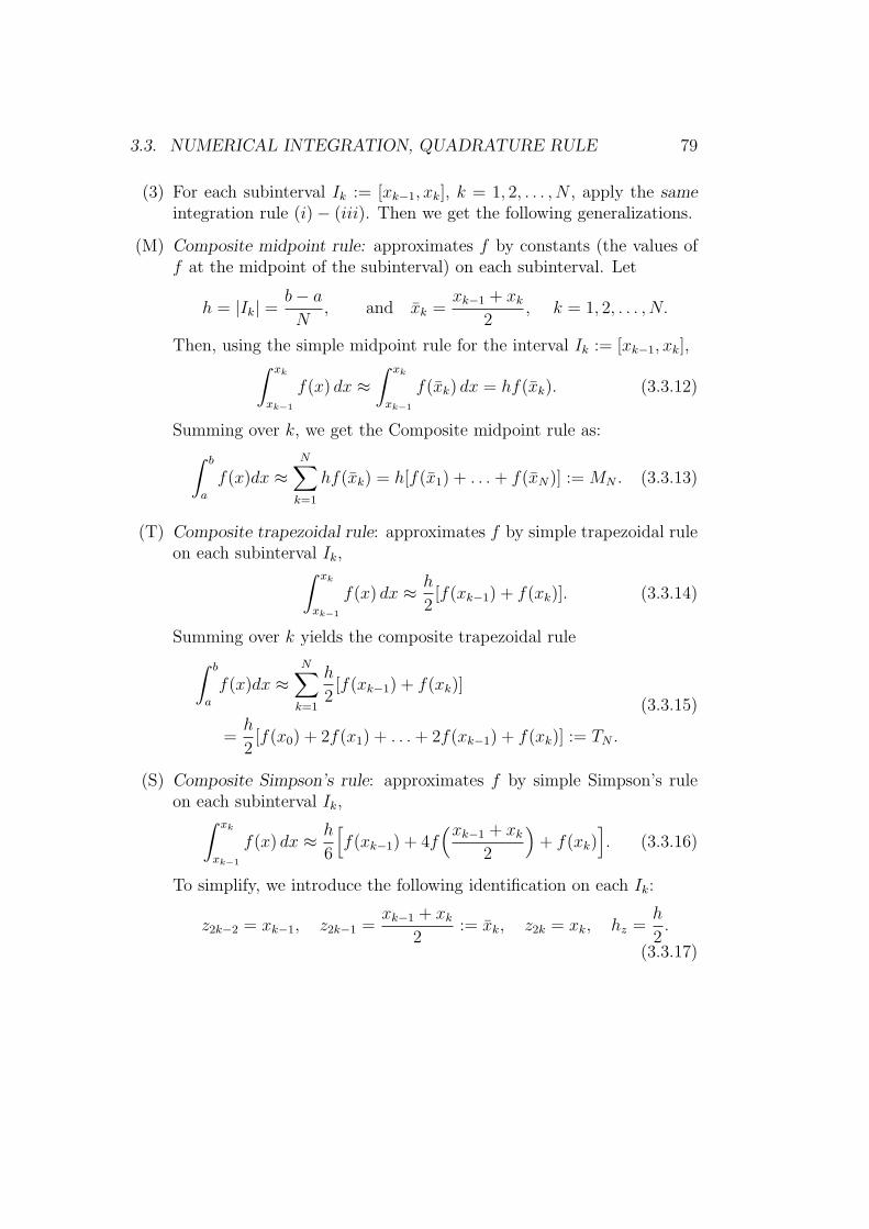
3.3. NUMERICAL INTEGRATION, QUADRATURE RULE 79
(3) For each subinterval Ik := [xk−1, xk], k = 1, 2, . . . , N , apply the sameintegration rule (i)− (iii). Then we get the following generalizations.
(M) Composite midpoint rule: approximates f by constants (the values off at the midpoint of the subinterval) on each subinterval. Let
h = |Ik| =b− a
N, and xk =
xk−1 + xk2
, k = 1, 2, . . . , N.
Then, using the simple midpoint rule for the interval Ik := [xk−1, xk],∫ xk
xk−1
f(x) dx ≈∫ xk
xk−1
f(xk) dx = hf(xk). (3.3.12)
Summing over k, we get the Composite midpoint rule as:
∫ b
a
f(x)dx ≈N∑
k=1
hf(xk) = h[f(x1) + . . .+ f(xN)] :=MN . (3.3.13)
(T) Composite trapezoidal rule: approximates f by simple trapezoidal ruleon each subinterval Ik,
∫ xk
xk−1
f(x) dx ≈ h
2[f(xk−1) + f(xk)]. (3.3.14)
Summing over k yields the composite trapezoidal rule
∫ b
a
f(x)dx ≈N∑
k=1
h
2[f(xk−1) + f(xk)]
=h
2[f(x0) + 2f(x1) + . . .+ 2f(xk−1) + f(xk)] := TN .
(3.3.15)
(S) Composite Simpson’s rule: approximates f by simple Simpson’s ruleon each subinterval Ik,
∫ xk
xk−1
f(x) dx ≈ h
6
[f(xk−1) + 4f
(xk−1 + xk2
)+ f(xk)
]. (3.3.16)
To simplify, we introduce the following identification on each Ik:
z2k−2 = xk−1, z2k−1 =xk−1 + xk
2:= xk, z2k = xk, hz =
h
2.
(3.3.17)

80CHAPTER 3. INTERPOLATION, NUMERICAL INTEGRATION IN 1D
< >
a = z0
a = x0
z1
x1
z2
x1
z2k−2
xk−1
z2k−1
xk
z2k
xk
z2N = b
xN = b
hz
Figure 3.8: Identification of subintervals for composite Simpson’s rule
Then, summing (3.3.16) over k and using the above identification, we obtainthe composite Simpson’s rule viz,
∫ b
a
f(x)dx ≈N∑
k=1
h
6
[f(xk−1) + 4f
(xk−1 + xk2
)+ f(xk)
]
=N∑
k=1
hz3
[f(z2k−2) + 4f(z2k−1) + f(z2k)
]
=hz3
[f(z0) + 4f(z1) + 2f(z2) + 4f(z3) + 2f(z4)
+ . . .+ 2f(z2N−2) + 4f(z2N−1) + f(z2N)]:= SN .
(3.3.18)
The figure below illustrates the starting procedure for the composite Simp-son’s rule. The numbers in the brackets indicate the actual coefficient oneach subinterval. For instance the end of the first interval : x1 = z2 coincideswith the start of the second interval, resulting to the add-up [1] + [1] = 2 asthe coefficient of f(z2). This is the case for each interior node xk which arez2k:s; for k = 1, . . . , N − 1.
Remark 3.4. One can verify that the errors of these integration rules aredepending on the regularity of the function and the size of interval (in simplerules) and the mesh size (in the composite rules). They read as follows:

3.3. NUMERICAL INTEGRATION, QUADRATURE RULE 81
z0
[1]
z1
[4]
z2
[1] + [1]
z3
[4]
z4
[1]
Figure 3.9: Coefficients for composite Simpson’s rule
Eroor in simple Midpoint rule
|∫ xk
xk−1
f(x) dx− hf(xk)| =h3
24|f ′′(η)|, η ∈ (xk−1, xk).
Error in composite Midpoint rule
|∫ b
a
f(x) dx−MN | =h2(b− a)
24|f ′′(ξ)|, ξ ∈ (a, b).
Error in simple trapezoidal rule
|∫ xk
xk−1
f(x) dx− h
2[f(xk−1 + f(xk)]| =
h3
12|f ′′(η)|, η ∈ (xk−1, xk).
Error in composite trapezoidal rule
|∫ b
a
f(x) dx− TN | =h2(b− a)
12|f ′′(ξ)|, ξ ∈ (a, b).
Error in simple Simpson’s rule
|∫ b
a
f(x) dx−b− a
6[f(a)+4f((a+b)/2)+f(b)]| = 1
90
(b− a
2
)5
|f (4)(η)|, η ∈ (a, b).
Error in composite Simpson’s rule
|∫ b
a
f(x) dx− SN | =h4(b− a)
180maxξ∈[a,b]
|f 4(ξ)|, h = (b− a)/N.
Remark 3.5. The rules (M), (T) and (S) use values of the function atequally spaced points. These are not always the best approximation methods.Below we introduce a general and more optimal approach.

82CHAPTER 3. INTERPOLATION, NUMERICAL INTEGRATION IN 1D
3.3.2 Gauss quadrature rule
This is an approximate integration rule aimed to choose the points of eval-uation of an integrand f in an optimal manner, not necessarily at equallyspaced points. Here, first we illustrate this rule by an example and thenconstruct and prove a general approach.
Problem: Choose the nodes xi ∈ [a, b], and coefficients ci, 1 ≤ i ≤ n suchthat, for an arbitrary integrable function f , the following error is minimal:
∫ b
a
f(x)dx−n∑
i=1
cif(xi). (3.3.19)
Solution. The relation (3.3.19) contains 2n unknowns consisting of n nodesxi and n coefficients ci. Therefore we need 2n equations. Thus if we replacef by a polynomial, then an optimal choice of these 2n parameters yields aquadrature rule (3.3.19) which is exact for polynomials, f , of degree ≤ 2n−1.
Example 3.5. Let n = 2 and [a, b] = [−1, 1]. Then the coefficients are c1 andc2 and the nodes are x1 and x2. Thus optimal choice of these 4 parametersshould yield that the approximation
∫ 1
−1
f(x)dx ≈ c1f(x1) + c2f(x2), (3.3.20)
is indeed exact for f(x) replaced by any polynomial of degree ≤ 3. So, wereplace f by a polynomial of the form f(x) = Ax3+Bx2+Cx+D and requireequality in (3.3.20). Thus, to determine the coefficients c1, c2 and the nodesx1, x2, in an optimal way, it suffices to change the above approximation toequality when f is replaced by the basis functions for polynomials of degree≤ 3: i.e. 1, x, x2 and x3. Consequently we get the equation system
∫ 1
−1
1dx = c1 + c2 and we get [x]1−1 = 2 = c1 + c2
∫ 1
−1
xdx = c1 · x1 + c2 · x2 and[x22
]1−1
= 0 = c1 · x1 + c2 · x2∫ 1
−1
x2dx = c1 · x21 + c2 · x22 and[x33
]1−1
=2
3= c1 · x21 + c2 · x22
∫ 1
−1
x3dx = c1 · x31 + c2 · x32 and[x44
]1−1
= 0 = c1 · x31 + c2 · x32,
(3.3.21)

3.3. NUMERICAL INTEGRATION, QUADRATURE RULE 83
which, although nonlinear, has the unique solution presented below:
c1 + c2 = 2
c1x1 + c2x2 = 0
c1x21 + c2x
22 =
23
c1x31 + c2x
32 = 0
=⇒
c1 = 1
c2 = 1
x1 = −√33
x2 =√33.
(3.3.22)
Hence, the approximation
∫ 1
−1
f(x)dx ≈ c1f(x1) + c2f(x2) = f(−
√3
3
)+ f
(√3
3
), (3.3.23)
is exact for all polynomials of degree ≤ 3.
Example 3.6. Let f(x) = 3x2 + 2x + 1. Then∫ 1
−1(3x2 + 2x + 1)dx =
[x3 + x2 + x]1−1 = 4, and we can easily check that f(−√3/3) + f(
√3/3) = 4.
Higher order Gauss quadrature. To generalize the Gauss quadraturerule, on an interval and to n > 2, Legendre polynomials are used. To illus-trate, we choose Pn∞n=0 such that
(1) For each n, Pn is a polynomial of degree n.
(2) Pn ⊥ Pm if m 6= n⇐⇒∫ 1
−1Pn(x)Pm(x)dx = 0.
The Legendre polynomials, on [−1, 1], can be obtained through the formula;(see Chapter 2, Overture),
Pn(x) =1
2nn!
dn
dxn
((x2 − 1)n
).
Here are the few first Legendre polynomials:
P0(x) = 1, P1(x) = x, P2(x) =3
2x2 − 1
2, P3(x) =
5
2x3 − 3
2x, . . . ,
The roots of Legendre polynomials are distinct, symmetric, with respect tox = 0, and the correct choices as quadrature points, i.e. the roots of theLegendre polynomial Pn (P0 = 1 is an exception) are our optimal quadraturepoints xi, 1 ≤ i ≤ n (viz, Theorem 3.5 below).

84CHAPTER 3. INTERPOLATION, NUMERICAL INTEGRATION IN 1D
Example 3.7. Roots of the Legendre polynomial as quadrature points:
P1(x) = x = 0.
P2(x) =3
2x2 − 1
2= 0, gives x1,2 = ±
√3
3. (compare with Example 3.5).
P3(x) =5
2x3 − 3
2x = 0, gives x1 = 0, x2,3 = ±
√3
5.
Theorem 3.6. Suppose that xi, i = 1, 2, . . . , n, are the roots of the n-thLegendre polynomial Pn and that
ci =
∫ 1
−1
n∏
j=1j 6=i
( x− xjxi − xj
)dx,
where
λi(x) =n∏
j=1j 6=i
( x− xjxi − xj
),
are the Lagrange basis functions with interpolation nodes xi. If we choose theabove (xi, ci) as nodes and coefficients (weights) of a Gauss quadrature rule
on [−1, 1], and if f(x) is a polynomial of degree < 2n, then
∫ 1
−1
f(x)dx ≡n∑
i=1
cif(xi), i.e. this quadrature approximation is exact for polynomials of
degree < 2n.
Proof. Consider a polynomial R(x) of degree < n. We can rewrite R(x) asa (n− 1)-th degree Lagrange interpolation polynomial with its nodes at theroots of the n-th Legendre polynomial Pn:
R(x) =n∑
i=1
n∏
j=1j 6=i
( x− xjxi − xj
)R(xi).
This representation of R(x) is exact, since for the error
E(x) =1
n!(x− x1)(x− x2) . . . (x− xn)R
(n)(ξ), we have R(n)(ξ) ≡ 0.
(3.3.24)

3.3. NUMERICAL INTEGRATION, QUADRATURE RULE 85
Integrating we get
∫ 1
−1
R(x)dx =
∫ 1
−1
[ n∑
i=1
n∏
j=1j 6=i
( x− xjxi − xj
)R(xi)
]dx
=n∑
i=1
[ ∫ 1
−1
n∏
j=1j 6=i
( x− xjxi − xj
)dx
]R(xi).
(3.3.25)
Hence, ∫ 1
−1
R(x)dx =n∑
i=1
ciR(xi), (3.3.26)
which shows the assertion of Theorem for polynomials of degree < n.Now consider a polynomial, P (x), of degree < 2n. Dividing P (x) by the
n-th Legendre polynomial Pn(x), we get
P (x) = Q(x)× Pn(x) +R(x), deg Q(x) < n, deg R(x) < n, (3.3.27)
and ∫ 1
−1
P (x)dx =
∫ 1
−1
Q(x)Pn(x)dx+
∫ 1
−1
R(x)dx. (3.3.28)
Since P0(x), P1(x), . . . , Pn−1(x) are basis functions for Pn−1(−1, 1), Q(x) ⊥Pn(x), ∀Q(x) with deg Q < n. Using (3.3.27) it follows that
∫ 1
−1
Q(x)Pn(x)dx = 0 =⇒∫ 1
−1
P (x)dx =
∫ 1
−1
R(x)dx. (3.3.29)
Recall that, the xi’s are the roots of Pn(x), i.e. Pn(xi) = 0. Thus, once againusing (3.3.27), we get
P (xi) = Q(xi)Pn(xi) +R(xi) = R(xi). (3.3.30)
Hence, by (3.3.29), (3.3.26) and (3.3.30),
∫ 1
−1
P (x)dx =
∫ 1
−1
R(x)dx =n∑
i=1
ciR(xi) =n∑
i=1
ciP (xi), (3.3.31)
and the proof is complete.

86CHAPTER 3. INTERPOLATION, NUMERICAL INTEGRATION IN 1D
3.4 Exercises
Problem 3.1. Use the expressions λa(x) = b−xb−a
and λb(x) = x−ab−a
to showthat
λa(x) + λb(x) = 1, aλa(x) + bλb(x) = x.
Give a geometric interpretation by plotting, λa(x), λb(x), λa(x) + λb(x),aλa(x), bλb(x) and aλa(x) + bλb(x).
Problem 3.2. Let f : [0.1] → R be a Lipschitz continuous function. De-termine the linear interpolant πf ∈ P(0, 1) and plot f and πf in the samefigure, when
(a) f(x) = x2, (b) f(x) = sin(πx).
Problem 3.3. Determine the linear interpolation of the function
f(x) =1
π2(x− π)2 − cos2(x− π
2), −π ≤ x ≤ π.
where the interval [−π, π] is divided into 4 equal subintervals.
Problem 3.4. Assume that w′ ∈ L1(I). Let x, x ∈ I = [a, b] and w(x) = 0.Show that
|w(x)| ≤∫
I
|w′|dx. (3.4.1)
Problem 3.5. Assume that v interpolates ϕ, at the points a and b.
h
v
ϕ
ax
b

3.4. EXERCISES 87
Show, using (3.4.1) that
(i) |(ϕ− v)(x)| ≤∫
I
|(ϕ− v)′| dx,
(ii) |(ϕ− v)′(x)| ≤∫
I
|(ϕ− v)′′| dx =
∫
I
|ϕ′′| dx,
(iii) maxI
|ϕ− v| ≤ maxI
|h2ϕ′′|,
(iv)
∫
I
|ϕ− v| dx ≤∫
I
|h2ϕ′′| dx,
(v) ‖ϕ− v‖I ≤ ‖h2ϕ′′‖I and ‖h−2(ϕ− v)‖I ≤ ‖ϕ′′‖I ,
where ‖w‖I =(∫
I
w2 dx)1/2
is the L2(I)-norm.
Problem 3.6. Use, in the above problem
v′ =ϕ(b)− ϕ(a)
h=
1
h
∫ b
a
ϕ′dx (ϕ′ is constant on I),
and show that
(vi) |(ϕ− v)(x)| ≤ 2
∫
I
|ϕ′| dx,
(vii)
∫
I
h−1|ϕ− v| dx ≤ 2
∫
I
|ϕ′| dx and ‖h−1(ϕ− v)‖ ≤ 2‖ϕ′‖I .
Problem 3.7. Let now v(t) be the constant interpolant of ϕ on I.
v
ϕ
xa b-

88CHAPTER 3. INTERPOLATION, NUMERICAL INTEGRATION IN 1D
Show that ∫
I
h−1|ϕ− v| dx ≤∫
I
|ϕ′| dx. (3.4.2)
Problem 3.8. Show that
Pq(a, b) := p(x)|p(x) is a polynomial of degree ≤ q,
is a vector space but
P q(a, b) := p(x)|p(x) is a polynomial of degree = q,
is not! a vector space.
Problem 3.9. Compute formulas for the linear interpolant of a continuousfunction f through the points a and (b+a)/2. Plot the corresponding Lagrangebasis functions.
Problem 3.10. Prove the following interpolation error estimate:
||π1f − f ||L∞(a,b) ≤1
8(b− a)2||f ′′||L∞(a,b).
Hint: Using an scaling argument, it suffices to prove the inequality for [a, b] ≡[0, 1].
Problem 3.11. Prove that any value of f on the sub-intervals, in a partitionof (a, b), can be used to define πhf satisfying the error bound
||f − πhf ||L∞(a,b) ≤ max1≤i≤m+1
hi||f ′||L∞(Ii) = ||hf ′||L∞(a,b).
Prove that choosing the midpoint improves the bound by an extra factor 1/2.
Problem 3.12. Compute and graph π4
(e−8x2
)on [−2, 2], which interpolates
e−8x2
at 5 equally spaced points in [−2, 2].
Problem 3.13. Write down a basis for the set of piecewise quadratic poly-nomials W
(2)h on a partition a = x0 < x1 < x2 < . . . < xm+1 = b of (a, b)
into subintervals Ii = (xi−1, xi), where
W(q)h = v : v|Ii ∈ Pq(Ii), i = 1, . . . ,m+ 1.

3.4. EXERCISES 89
Problem 3.14. Determine a set of basis functions for the space of continuouspiecewise quadratic functions V
(2)h on I = (a, b), where
V(q)h = v ∈ W
(q)h : v is continuous on I.
Problem 3.15. Prove that∫ x1
x0
f ′(x1 + x0
2
)(x− x1 + x0
2
)dx = 0.
Problem 3.16. Prove that
∣∣∣∫ x1
x0
f(x) dx− f(x1 + x0
2
)(x1 − x0)
∣∣∣
≤ 1
2max[x0,x1]
|f ′′|∫ x1
x0
(x− x1 + x0
2
)2
dx ≤ 1
24(x1 − x0)
3 max[x0,x1]
|f ′′|.
Hint: Use Taylor expansion of f about x = x1+x0
2.

90CHAPTER 3. INTERPOLATION, NUMERICAL INTEGRATION IN 1D

Chapter 4
Linear Systems of Equations
We have seen that the numerical solution of a differential equation, e.g. usingthe Galerkin finite element method, is an approximation of the exact solutionwith a function in a finite dimensional vector space. If the differential equation islinear (see the Definition 1.3), then the procedure ends solving a linear system ofequations of the form Ax = b, where the coefficient matrix A is a square matrixof the same order as the dimension of the approximation space, and is relatedto the differential operator in the equation, x is a vector in the approximationspace with entries consisting of certain nodal values of the approximate solution,and the vector b is related to the data and basis functions of the approximationspace.
The criterion for the quality of a numerical method, to solve a certain prob-lem, lies in its potential in speed (rate) of convergence of the approximate solutionto the exact one in an adequate measuring environment (norm). Quantitatively,this is expressed by “how fast” the approximate solution would converge to theexact solution by increasing the approximation degree (the dimension of the ap-proximation space), which is a theoretical procedure. In computations however,with an already justified convergence, it is important to have a numerical algo-rithm that solves the approximate problem reasonably fast (takes shorter timewhich may be achieved, e.g. by taking a fewer number of approximation points).
This chapter is devoted to the numerical solution of linear systems ofequations of type Ax = b. Throughout this chapter we assume that detA 6=0, i.e. the matrix A is invertible. Then Ax = b ⇔ x = A−1b, but we wishto circumvent inverting the matrix A. To this approach we shall review the
91

92 CHAPTER 4. LINEAR SYSTEMS OF EQUATIONS
well-known direct method of Gauss elimination and then continue with somemore efficient iterative approaches. A thorough study of this type is in therealm of numerical linear algebra where the solution algorithms for linearsystems of equations is undoubtedly one of the most applied tools.
4.1 Direct methods
Consider the general form of an n× n linear system of equations given by
Ax = b ⇔ ∑nj=1 aijxj = bi,
i = 1, . . . , n,or
a11x1 + a12x2 + . . .+ a1nxn = b1
a21x1 + a22x2 + . . .+ a2nxn = b2
. . .
an1x1 + an2x2 + . . .+ annxn = bn.
We introduce the extended n × (n + 1) coefficient matrix E consisting ofthe coefficient matrix A enlarged by putting the right hand side b as theadditional last column:
E :=
a11 a12 . . . a1n b1
a21 a22 . . . a2n b2
. . . . . . . . . . . . . . .
an1 an2 . . . ann bn
. (4.1.1)
Note that to solve the equation system Ax = b, it is a bad idea to calculateA−1 and then multiply by b. However, if A is an upper (or lower) triangularmatrix, i.e., if aij = 0 for i > j (or i < j), and A is invertible, then we can

4.1. DIRECT METHODS 93
solve x using the back substitution method:
a11x1 + a12x2 + . . .+ a1nxn = b1
a22x2 + . . .+ a2nxn = b2
. . . . . . . . .
. . . . . . . . .
an−1,n−1xn−1 + an−1,nxn = bn−1
annxn = bn,
(4.1.2)
which yields
x1 =1
a11[b1 − a12x2 − . . .− a1nxn]
. . . . . . . . .
. . . . . . . . .
xn−1 =1
an−1,n−1
[bn−1 − an−1,nxn]
xn =bnann
.
(4.1.3)
Number of operations. The speed of convergence depends on the numberof operations performed during the computations. In the above procedureadditions and subtractions are not considered as time consuming operations,therefore we shall count only the number of multiplications and divisions.• The number of multiplications to solve for xn from (4.1.3) is zero and thenumber of divisions is one.• To solve for xn−1 we need one multiplication and one division.• To solve for x1 we need (n− 1) multiplication and one division.Thus to solve the triangular linear system of equations given by (4.1.2) weshall need
1 + 2 + . . .+ (n− 1) =n(n− 1)
2:=
n2
2+Q(n),
multiplications, where Q(n) is a remainder of order n, and n divisions.

94 CHAPTER 4. LINEAR SYSTEMS OF EQUATIONS
Gaussian elimination method. This method is based on the followingobvious facts expressing that: a solution to a linear system of equations isnot changed under elementary row operations. These are
(i) interchanging two equations
(ii) adding a multiple of one equation to another
(iii) multiplying an equation by a nonzero constant.
The Gauss elimination procedure is based on splitting the coefficient matrixA to two factors, an upper triangular matrix U and a lower triangular matrixL, known as LU factorization. Below are examples of 3×3 dimensional uppertriangular matrix U , lower triangular matrix L and diagonal matrix D,
U =
a b c
0 d e
0 0 f
, L =
a 0 0
g d 0
h i f
, D =
a 0 0
0 d 0
0 0 f
.
Of course some of the entries a, b, . . . , i above may also be zero. To performthe Gauss elimination procedure, we start from the first row of the coefficientmatrix of the equation system and use elementary row operations to eliminatethe elements ai1, i > 1, under a11 (make ai1 = 0).
Remark 4.1. If a11 = 0, then we interchange equations, and replace the firstequation by an equation in the system with ai1 6= 0.
The equation system corresponding to this newly obtained matrix A withelements aij, and where ai1 = 0, i > 1, has the same solution as the originalone. We repeat the same procedure of elementary row operations to eliminatethe elements ai2, i > 2, from the matrix A. Continuing in this way, we obtainan upper triangular matrix U with a corresponding equation system whichis equivalent to the original system (has the same solution). Below we shallillustrate this procedure through an example.
Example 4.1. Solve the linear system of equations
2x1 + x2 + x3 = 2
4x1 − x2 + 3x3 = 0
2x1 + 6x2 − 2x3 = 10.
(4.1.4)

4.1. DIRECT METHODS 95
In the extended coefficient matrix:
E =
2 1 1 | 2
4 −1 3 | 0
2 6 −2 | 10
, (4.1.5)
we have that a11 = 2, a21 = 4, and a31 = 2. We introduce the multipliersmi1, i > 1 by letting
m21 =a21a11
=4
2= 2 m31 =
a31a11
=2
2= 1. (4.1.6)
Now we multiply the first row by m21 and then subtract it from row 2 andreplace the result in row 2:
2 1 1 | 2
4 −1 3 | 0
2 6 −2 | 10
·(−2)
=⇒
2 1 1 | 2
0 −3 1 | −4
2 6 −2 | 10
(4.1.7)
Similarly we multiply the first row by m31 = 1, subtract it from row 3, andreplace the result in row 3:
E :=
2 1 1 | 2
0 −3 1 | −4
0 5 −3 | 8
. (4.1.8)
In this setting we have a22 = −3 and a32 = 5. Now we let m32 = a32/a22 =−5/3, then multiplying the second row in E by m32 and subtracting the resultfrom row 3 yields
2 1 1 | 2
0 −3 1 | −4
0 0 −4
3| 4
3
, (4.1.9)

96 CHAPTER 4. LINEAR SYSTEMS OF EQUATIONS
where we have obtained the upper triangular matrix
U =
2 1 1
0 −3 1
0 0 −4
3
. (4.1.10)
The new equivalent equation system is
2x1 + x2 + x3 = 2
−3x2 + x3 = −4
−4
3x3 =
43
(4.1.11)
with the solution x1 = 1, x2 = 1 and x3 = −1 which, as we can verify, isalso the solution of the original equation system (4.1.4).
Remark 4.2. For an n×n matrix A, the number of operation in the Gausselimination procedure, leading to an upper triangular matrix U , is of orderO(n3). Recall that the number of operations to solve an n×n upper triangularsystem is O(n2). Therefore the total number of operations to solve an n× nlinear system of equations using the Gauss elimination is of order O(n3).
Definition 4.1. We define the lower triangular matrices:
L1 =
1 0 0
−m21 1 0
−m31 0 1
, L2 =
1 0 0
0 1 0
0 −m32 1
and L =
1 0 0
m21 1 0
m31 m32 1
,
where m21, m31 and m32 are the multipliers. The matrices L1, L2 and L areunit (ones on the diagonal) lower triangular 3× 3-matrices with the propertythat
L = (L2L1)−1 = L−1
1 L−12 , and A = LU. (4.1.12)
Example 4.2. Continuing the previous example, we have m21 = 2,m31 = 1and m32 = −5/3, consequently

4.1. DIRECT METHODS 97
L1 =
1 0 0
−2 1 0
−1 0 1
, L2 =
1 0 0
0 1 0
05
31
and L =
1 0 0
2 1 0
1 −5
31
.
Thus
L1A =
1 0 0
−2 1 0
−1 0 1
2 1 1
4 −1 3
2 6 −2
=
2 1 1
0 −3 1
0 5 −3
= A,
which corresponds to the first two elementary row operations in the Gaussianelimination. Further
L2L1A =
1 0 0
0 1 0
05
31
2 1 1
0 −3 1
0 5 −3
=
2 1 1
0 −3 1
0 0 −4
3
= U,
which corresponds to the last (third) elementary row operation performed inthe previous example.
Note that, the last relation means also
A = (L2L1)−1U = LU.
In the general setting we have the following result:
Proposition 4.1. The n× n unit lower triangular matrix L is given by
L = (Ln−1Ln−2 . . . L1)−1,
where Li, i = 1, . . . , n−1 are the corresponding n×n row-operation matrices,viz example above. For n = 3 we have (L2L1)
−1 = L, where
L =
1 0 0
m21 1 0
m31 m32 1
,
and mij are the multipliers defined above.

98 CHAPTER 4. LINEAR SYSTEMS OF EQUATIONS
LU factorization of an n× n matrix A
To generalize the above procedure from the 3 × 3 case, to an n × n linearsystem of equations we use the factorization A = LU of the coefficient matrixA, where L is a unit lower triangular matrix and U is an upper triangularmatrix obtained from A by Gaussian elimination.To solve the system Ax = b, assuming we have an LU factorization, we lety = Ux, and first solve Ly = b by forward substitution (from the first rowto the last) and obtain the vector y, then using y as the known right handside finally we solve Ux = y by backward substitution (from the last row tothe first) and get the solution x.
Thus
Ax = b ⇐⇒ (LU)x = b ⇐⇒ L(Ux) = b
⇐⇒ (Ly = b ∧ Ux = y).
Observe that, in the Gauss elimination procedure, Ly = b is solved “byautomatic”, viz
y = L−1b = L2L1b.
Then, we solve
Ux = L2L1Ax = L2L1b = L−1b = y,
by backward substitution.
Below we illustrate this procedure through an example.
Example 4.3. We return to the previous example where we have that
L =
1 0 0
2 1 0
1 −5
31
and b =
2
0
10
.
• Ly = b yields the system of equations
1 0 0
2 1 0
1 −5
31
y1
y2
y3
=
2
0
10
⇐⇒
y1 = 2
2y1 + y2 = 0
y1 −5
3y2 + y3 = 10.

4.1. DIRECT METHODS 99
Using forward substitution we get y1 = 2, y2 = −4, y3 = 4/3. Further with
U =
2 1 1
0 −3 1
0 0 −4
3
and y =
2
−44
3
.
• Ux = y yields
2 1 1
0 −3 1
0 0 −4
3
x1
x2
x3
=
2
−44
3
⇐⇒
2x1 + x2 + x3 = 2
− 3x2 + x3 = −4
−4
3x3 =
4
3.
Using backward substitution, we get the solution: x1 = 1, x2 = 1, x3 = −1.
Remark 4.3. In some cases we can predict the solubility of an equationsystem: Let A be an n× n matrix. Then we have the following properties:• If det(A) 6= 0, then the system of equations Ax = b has a unique solution,given by x = A−1b.• A has an LU factorization if det(∆k) 6= 0, k = 1, . . . , n− 1, where ∆k isSylvester’s matrix:
∆k =
a11 . . . a1k
. . . . . . . . .
ak1 . . . akk
.
• If the LU factorization exists and det(A) 6= 0, then the LU factorization isunique and det(A) = U11 · . . . · Unn.
In particular for the “symmetric matrices” we have:
Theorem 4.1 (Cholesky’s method). Let A be a symmetric matrix, (aij =aji), then the following statements are equivalent:
(i) A is positive definite.
(ii) The eigenvalues of A are positive.
(iii) Sylvester’s criterion: det(∆k) > 0 for k = 1, 2, . . . , n.

100 CHAPTER 4. LINEAR SYSTEMS OF EQUATIONS
(iv) A = LLT where L is lower triangular and has positive diagonal ele-ments. (Cholesky factorization)
We do not give a proof of this theorem. The interested reader is referredto literature in linear algebra and matrix theory, e.g. G. Golub [24].
4.2 Iterative methods
To speed up the solution procedure, instead of solving Ax = b directly,for the exact solution x, we consider iterative solution methods based oncomputing a sequence of approximations x(k), k = 1, 2, . . . such that
limk→∞
x(k) = x or limk→∞
‖x(k) − x‖ = 0, for some matrix norm.
Example 4.4. For an n×n matrix A, L1 and L∞ matrix norms are definedby
||A||1 = maxj
n∑
i=1
|aij|,
||A||∞ = maxi
n∑
j=1
|aij|.
Thus consider the general n×n linear system of equations Ax = b, whereboth the coefficient matrix A and the vector b have real entries,
Ax = b ⇐⇒
a11x1 +a12x2 + . . . +a1nxn = b1
a2,1x1 +a22x2 . . . +a2nxn = b2
. . . . . . + . . . . . . . . .
an1x1 + . . . + . . . +annxn = bn.
(4.2.1)
For the system (4.2.1) we shall introduce the two main iterative methods.

4.2. ITERATIVE METHODS 101
Jacobi iteration: Assume that aii 6= 0, then (4.2.1) can be rewritten as:
x1 = − 1
a11[a12x2 + a13x3 + . . .+ a1nxn − b1]
x2 = − 1
a22[a21x1 + a23x3 + . . .+ a2nxn − b2]
. . .
xn = − 1
ann[an1x1 + an2x2 + . . .+ an,n−1xn−1 − bn].
We start with a given initial approximation for the solution, viz
x(0) = (x(0)1 = c1, x
(0)2 = c2, . . . , x
(0)n = cn),
and, based on the above system, define a successive iteration procedure, fork = 0, 1, 2, . . . , as:
x(k+1)1 = − 1
a11[a12x
(k)2 + a13x
(k)3 + . . .+ a1nx
(k)n − b1]
x(k+1)2 = − 1
a22[a21x
(k)1 + a23x
(k)3 + . . .+ a2nx
(k)n − b2]
. . . . . . . . .
x(k+1)n = − 1
ann[an1x
(k)1 + an2x
(k)2 + . . .+ an,n−1x
(k)n−1 − bn],
or in compact form in Jacobi coordinates, by
n∑
j=1
aijxj = bi ⇐⇒ aiixi = −n∑
j=1j 6=i
aijxj + bi,
aiix(k+1)i = −
n∑
j=1j 6=i
aijx(k)j + bi.
(4.2.2)
If n is large and the number of iterations are small (< n), then the Jacobimethod requires less operations than the usual Gauss elimination method.Below we state a convergence criterion (the proof is left as an exercise).

102 CHAPTER 4. LINEAR SYSTEMS OF EQUATIONS
Convergence criterion:The Jacobi method gives convergence to the exact solution if the matrix Ais strictly diagonally dominant, i.e.
|aii| >n∑
j=1j 6=i
|aij| i = 1, 2, . . . , n. (4.2.3)
Problem 4.1. Show that A =
4 2 1
1 5 1
0 1 3
is diagonally dominant.
Example 4.5. Solve Ax = b where A =
2 −1
−1 2
and b =
1
1
.
A is diagonally dominant and the matrix equation Ax = b is equivalent tothe linear equation system
2x1 − x2 = 1
−x1 + 2x2 = 1.(4.2.4)
We choose zero initial values for x1 and x2, i.e. x(0)1 = 0 and x
(0)2 = 0 and
use (4.2.4) to build the Jacobi iteration system
2x(k+1)1 = x
(k)2 + 1
2x(k+1)2 = x
(k)1 + 1,
(4.2.5)
where k is the iteration step. Then we have
2x(1)1 = x
(0)2 + 1
2x(1)2 = x
(0)1 + 1
with the solution
x(1)1 = 1/2
x(1)2 = 1/2.
(4.2.6)
In the next iteration step:
2x(2)1 = x
(1)2 + 1
2x(2)2 = x
(1)1 + 1
⇒
2x(2)1 = 1/2 + 1
2x(2)2 = 1/2 + 1
⇒
x(2)1 = 3/4
x(2)2 = 3/4.
(4.2.7)

4.2. ITERATIVE METHODS 103
Continuing we obviously have limk→∞
x(k)i = xi, i = 1, 2, where x1 = x2 = 1.
Below we show the first few iterations giving the corresponding x(k)1 and x
(k)2
values
k x(k)1 x
(k)2
0 0 0
1 1/2 1/2
2 3/4 3/4
3 7/8 7/8
Now if we use the maximum norm: ‖ek‖∞ := maxi=1,2
|x(k)i − xi|, then
‖e0‖∞ = max(|x(0)1 − x1|, |x(0)2 − x2|) = max(∣∣∣0− 1
∣∣∣,∣∣∣0− 1
∣∣∣)= 1
‖e1‖∞ = max(|x(1)1 − x1|, |x(1)2 − x2|) = max(∣∣∣
1
2− 1
∣∣∣,∣∣∣1
2− 1
∣∣∣)=
1
2
‖e2‖∞ = max(|x(2)1 − x1|, |x(2)2 − x2|) = max(∣∣∣
3
4− 1
∣∣∣,∣∣∣3
4− 1
∣∣∣)=
1
4
‖e3‖∞ = max(|x(3)1 − x1|, x(3)2 − x2|) = max(∣∣∣
7
8− 1
∣∣∣,∣∣∣7
8− 1
∣∣∣)=
1
8.
In this way ‖ek+1‖∞ =1
2‖ek‖∞, where ek is the error in step k ≥ 0. Iterating,
we see that for the k-th Jacobi iteration the convergence rate is(12
)k
:
‖ek‖∞ =1
2‖ek−1‖∞ =
(12
)2
‖ek−2‖∞ = . . . =(12
)k
‖e0‖∞ =(1/2
)k
.
Gauss-Seidel iterationWe start again with an initial approximation of the solution of the form
x ≈(x(0)1 , x
(0)2 , . . . , x(0)n
).

104 CHAPTER 4. LINEAR SYSTEMS OF EQUATIONS
Here we use the fact that the first row in the k-th Jacobi iteration givesx(k+1)1 and in the i+1-th row x
(k+1)1 , . . . , x
(k+1)i are already computed values
given on the left hand sides of the previous (first i) rows. Then, the ideain the Gauss-Seidel procedure is: that, in the very same iteration step, onesimultaneously inserts these previously computed values. More specificallythe Gauss-Seidel iteration steps are given by:
x(k+1)1 =
−1
a11[a12x
(k)2 + a13x
(k)3 + . . .+ a1nx
(k)n − b1]
x(k+1)2 =
−1
a22[a21x
(k+1)1 + a23x
(k)3 + . . .+ a2nx
(k)n − b2]
. . .
x(k+1)n−1 =
−1
an−1,n−1
[an−1,1x(k+1)1 + . . .+ an−1,n−2x
(k+1)n−2 + an−1,nx
(k)n − bn−1]
x(k+1)n =
−1
ann[an1x
(k+1)1 + an2x
(k+1)2 + . . .+ an,n−1x
(k+1)n−1 − bn],
or in a compact form in Gauss-Seidel coordinates, as
Ax = b ⇐⇒n∑
j=1
aijxj = bi ⇐⇒i∑
j=1
aijxj +n∑
j=i+1
aijxj = bi. (4.2.8)
Therefore the iterative form for the Gauss-Seidel method is given by
∑ij=1 aijx
(k+1)j = −
∑nj=i+1 aijx
(k)j + bi ⇐⇒
aiix(k+1)i = −∑i−1
j=1 aijx(k+1)j −∑n
j=i+1 aijx(k)j + bi.
(4.2.9)
Example 4.6. We consider the same example as above: Ax = b with
A =
2 −1
−1 2
, x =
x1
x2
, and b =
1
1
.
Recall the Jacobi iteration system
2x(k+1)1 = x
(k)2 + 1,
2x(k+1)2 = x
(k)1 + 1.
(4.2.10)

4.2. ITERATIVE METHODS 105
The corresponding Gauss-Seidel iteration system reads as follows:
2x(k+1)1 = x
(k)2 + 1,
2x(k+1)2 = x
(k+1)1 + 1.
(4.2.11)
We choose the same initial values for x1 and x2 as in the Jacobi iterations,i.e. x
(0)1 = 0, and x
(0)2 = 0. Now the first equation in (4.2.11):
2x(1)1 = x
(0)2 + 1 =⇒ x
(1)1 =
1
2.
Inserting this value of x(1)1 = 1
2into the second equation in (4.2.11) yields
2x(1)2 = x
(1)1 + 1 =⇒ 2x
(1)2 =
1
2+ 1 =⇒ x
(1)2 =
3
4.
Below we list the first few iteration steps for this Gauss-Seidel approach:
k x(k)1 x
(k)2
0 0 0
1 1/2 3/4
2 7/8 15/16
3 31/32 63/64
Obviously limk→∞
x(k)1 = lim
k→∞x(k)2 = 1. Now with ‖ek‖∞ = max
i=1,2|x(k)i − xi|, we
get the successive iteration errors:
‖e1‖∞ = max(|x(1)1 − x1|, |x(1)2 − x2|) = max(∣∣∣
1
2− 1
∣∣∣,∣∣∣3
4− 1
∣∣∣)=
1
2
‖e2‖∞ = max(∣∣∣
7
8− 1
∣∣∣,∣∣∣15
16− 1
∣∣∣)=
1
8, ‖e3‖∞ = max
( 1
32,1
64
)=
1
32.
Thus for the Gauss-Seidel iteration ‖ek+1‖∞ =1
4‖ek‖∞, where ek is the error
for step k, and hence we can conclude that the Gauss-Seidel method convergesfaster than the Jacobi method:
‖ek‖∞ =1
4‖ek−1‖∞ =
(14
)2
‖ek−2‖∞ = · · · =(14
)k
‖e0‖∞ =(14
)k
.

106 CHAPTER 4. LINEAR SYSTEMS OF EQUATIONS
The successive over-relaxation method (S.O.R.).The S.O.R. method is a modified version of the Gauss-Seidel iteration. Theiteration procedure is given by
x(k+1)i = (1− ω)x
(k)i +
ω
aii
[bi −
i−1∑
j=1
aijx(k+1)j −
n∑
j=i+1
aijx(k)j
](4.2.12)
For ω > 1 the method is called an over-relaxation method and if 0 < ω < 1,it is referred to as an under-relaxation method. In the S.O.R. coordinateswe have
aiix(k+1)i = aiix
(k)i − ω
( i−1∑
j=1
aijx(k+1)j +
n∑
j=i
aijx(k)j − bi
). (4.2.13)
Remark 4.4. Note that for ω = 1, (4.2.13) gives the Gauss-Seidel method.
Abstraction of iterative methodsIn our procedures we have considered Ax = b and x = Bx+ c as equivalentlinear systems of equations, where B is the iteration matrix and xk+1 =Bxk + c.
Some advantages of iterative methods over direct methods are:(i) Iterative methods are faster (depends on B, accuracy is required)(ii) Iterative methods require less memory (sparsity of A can be preserved).
By a spars matrix we mean a matrix with most zero elements, i.e. amatrix that has very few non-zero elements.
Questions: For a qualitative study of an iteration procedure the followingquestions are of vital interest;
(Q1) For a given A, what is a good choice for B?(Q2) When does x(k) → x?(Q3) What is the rate of convergence?
The error at step k is ek = x(k)−x and that of step (k+1) is ek+1 = x(k+1)−x.Then we have ek+1 = x(k+1)−x = (Bx(k)+c)−(Bx+c) = B(x(k)−x) = Bek.Iterating, we have
ek = Bek−1 = B ·Bek−2 = B3ek−3 = . . . = Bkek−k = Bk e0.

4.2. ITERATIVE METHODS 107
Thus we have shown that ek = Bke0. Let now
L =
0 . . . . . . 0
a21 0 . . . 0
. . . . . . . . . . . .
an1 . . . an,n−1 0
, U =
0 a12 . . . a1n
. . . . . . . . . . . .
. . . . . . 0 an−1,n
0 . . . . . . 0
and
D =
a11 0 . . . 0
0 a22 0 . . .
. . . . . . . . . . . .
0 . . . 0 ann
,
then A = L + D + U . We can rewrite Ax = b as (L + D + U)x = b thenDx = −(L + U)x + b, and we may reformulate the iterative methods asfollows.
Jacobi’s method
Dx(k+1) = −(L+ U)x(k) + b ⇒ BJ = −D−1(L+ U),
where BJ is the Jacobi iteration matrix.
Example 4.7. We consider the previous example and write the linear system

108 CHAPTER 4. LINEAR SYSTEMS OF EQUATIONS
in matrix form as x = BJx+ c, i.e.
2x1 − x2 = 1
−x1 + 2x2 = 1⇒
x1 =1
2x2 +
1
2
x2 =1
2x1 +
1
2
which in matrix form is
x1
x2
=
0 1
2
12
0
x1
x2
+
12
12
, where
x =
x1
x2
, BJ =
0 1
2
12
0
and c =
12
12
.
Example 4.8. Determine the same matrix BJ by the formula:BJ = −D−1(L+ U),
A =
2 −1
−1 2
, L =
0 0
−1 0
, U =
0 −1
0 0
, D =
2 0
0 2
.
We can easily see that
D−1 =1
2
1 0
0 1
,
and thus
BJ = −D−1(L+ U) = −1
2
1 0
0 1
0 −1
−1 0
=
1
2
0 1
1 0
.
Gauss-Seidel’s methodAs in the Jacobi case, we may write Ax = b as (L+D + U)x = b but nowwe choose (L+D)x = −Ux+ b. Similar to the previous procedure we thenhave (L + D)x(k+1) = −Ux(k) + b, and then BGS = −(L + D)−1U , whereBGS stands for the Gauss-Seidel iteration matrix.

4.3. EXERCISES 109
RelaxationGauss-Seidel corresponds to (L+D)x = −Ux+ b, thus the iteration proce-dure is:
Dx(k+1) = Dx(k) − [Lx(k+1) + (D + U)x(k) − b].
Now we define the general relaxation procedure
x(k+1) = (1− ω)x(k) + ωD−1(b− Lx(k+1) − Ux(k)
), (4.2.14)
where the coefficient of ω, in the second term, is just the right hand side ofGauss-Seidel’s method: the term in the bracket in (4.2.12). We may rewrite(4.2.14) as
(ωL+D)x(k+1) = [(1− ω)D − ωU ]x(k) + ωb,
where ω is the relaxation parameter, (ω = 1 gives the Gauss-Seidel iteration).Thus the relaxation iteration matrix is:
Bω = (ωL+D)−1[(1− ω)D − ωU ].
4.3 Exercises
Problem 4.2. Illustrate the LU factorization for the matrix
A =
1 3 2
−2 −6 1
2 5 7
.
Problem 4.3. Solve A4x = b for
A =
−1 2
2 −3
b =
144
−233
Problem 4.4. Find the unique LDU factorization for the matrix
A =
1 1 −3
0 1 1
3 −1 1
.

110 CHAPTER 4. LINEAR SYSTEMS OF EQUATIONS
Hint: First find the LU factorization of A. Then D is a diagonal matrixwith its diagonal elements being those of U . U is an upper triangular matrixobtained from U by replacing the diagonal elements of U by ones.
Problem 4.5. Show that every orthogonal 2× 2 matrix is of the form
A1 =
c s
−s c
or A2 =
c s
s −c
,
where c2 + s2 = 1
Problem 4.6. Find the LU factorization for the matrix A
A =
1 1 0 0
1 3 1 0
0 2 4 1
0 0 3 5
.
Problem 4.7. Solve the following system of equations 4 −1
−1 4
u1
u2
=
1
−3
using the following iteration methods and a starting value of u0 = (0, 0)T .(a) Jacobi Method.(b) Gauss-Seidel Method.(c) Optimal SOR (you must compute the optimal value of ω = ω0 first).
Problem 4.8. Prove strict diagonal dominance (4.2.3) implies convergenceof Jacobi and Gauss-Seidel methods.
Hint: One may use fix-point iterations.
Problem 4.9. A is an orthogonal matrix if ATA = I (I being the identitymatrix). Show that for any vector v with ||v||2 = 1, the matrix I − vvT isorthogonal.
Problem 4.10. Suppose that det(aij) = 0, but aii 6= 0 for all i. Prove thatthe Jacobi’s method does not converge.
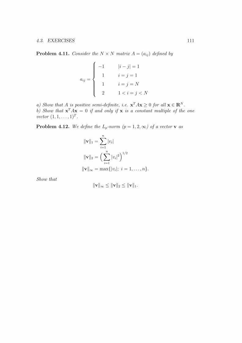
4.3. EXERCISES 111
Problem 4.11. Consider the N ×N matrix A = (aij) defined by
aij =
−1 |i− j| = 1
1 i = j = 1
1 i = j = N
2 1 < i = j < N
a) Show that A is positive semi-definite, i.e. xTAx ≥ 0 for all x ∈ RN .b) Show that xTAx = 0 if and only if x is a constant multiple of the onevector (1, 1, . . . , 1)T .
Problem 4.12. We define the Lp-norm (p = 1, 2,∞) of a vector v as
‖v‖1 =n∑
i=1
|vi|
‖v‖2 =( n∑
i=1
|vi|2)1/2
‖v‖∞ = max|vi|; i = 1, . . . , n.
Show that‖v‖∞ ≤ ‖v‖2 ≤ ‖v‖1.
112 CHAPTER 4. LINEAR SYSTEMS OF EQUATIONS

Chapter 5
Two-point boundary valueproblems
In this chapter we focus on finite element approximation procedure for two-point boundary value problems (BVPs). For each problem we formulate acorresponding variational formulation (VF) and a minimization problem (MP)and prove that the solution to either of BVP, its VF and MP satisfies the othertwo as well.
(BV P ) ” ⇐⇒ ” (V F ) ⇐⇒ (MP ).
We also prove a priori and a posteriori error estimates. The ⇐= in theequivalence ” ⇐⇒ ” is subject to a regularity requirement on the solution up tothe order of the underlying PDE.
5.1 A Dirichlet problem
Assume that a horizontal elastic bar which occupies the interval I := [0, 1],is fixed at the end-points. Let u(x) denote the displacement of the bar at apoint x ∈ I, a(x) be the modulus of elasticity, and f(x) a given load function,then one can show that u satisfies the following boundary value problem
(BV P )1
−(a(x)u′(x)
)′= f(x), 0 < x < 1,
u(0) = u(1) = 0.(5.1.1)
Equation (5.1.1) is of Poisson’s type modelling also the stationary heat flux(1.2.6) derived in Chapter 1.
113

114 CHAPTER 5. TWO-POINT BOUNDARY VALUE PROBLEMS
We shall assume that a(x) is piecewise continuous in (0, 1), bounded for0 ≤ x ≤ 1 and a(x) > 0 for 0 ≤ x ≤ 1.
Let v(x) and its derivative v′(x), x ∈ I, be square integrable functions,that is: v, v′ ∈ L2(0, 1), and define the L2-based Sobolev space by
H10 (0, 1) =
v :
∫ 1
0
(v(x)2 + v′(x)2)dx <∞, v(0) = v(1) = 0. (5.1.2)
The variational formulation (VF). We multiply the equation in (BVP)1by a so called test function v ∈ H1
0 (0, 1) and integrate over (0, 1) to obtain
−∫ 1
0
(a(x)u′(x))′v(x)dx =
∫ 1
0
f(x)v(x)dx. (5.1.3)
Using integration by parts we get
−[a(x)u′(x)v(x)
]10+
∫ 1
0
a(x)u′(x)v′(x)dx =
∫ 1
0
f(x)v(x)dx. (5.1.4)
Now since v(0) = v(1) = 0 we have thus obtained the variational formulationfor the problem (5.1.1) as follows: find u ∈ H1
0 such that
(VF)1
∫ 1
0
a(x)u′(x)v′(x)dx =
∫ 1
0
f(x)v(x)dx, ∀v ∈ H10 . (5.1.5)
In other words we have shown that if u satisfies (BVP)1, then u also satisfiesthe (VF)1 above. We write this as (BVP)1 =⇒ (VF)1. Now the questionis whether the reverse implication is true, i.e. under which conditions canwe deduce the implication (VF)1 =⇒ (BVP)1? It appears that this questionhas an affirmative answer, provided that the solution u to (VF)1 is twicedifferentiable. Then, modulo this regularity requirement, the two problemsare indeed equivalent. We prove this in the following theorem.
Theorem 5.1. The following two properties are equivalent
i) u satisfies (BVP)1
ii) u is twice differentiable and satisfies (VF)1.
Proof. We have already shown (BVP)1 =⇒ (VF)1.It remains to show that (VF)1 =⇒ (BVP)1:

5.1. A DIRICHLET PROBLEM 115
Integrating by parts on the left hand side in (5.1.5), assuming that u is twicedifferentiable, and using f ∈ C(0, 1), a ∈ C1(0, 1) and v(0) = v(1) = 0 wereturn to the relation (5.1.3):
−∫ 1
0
(a(x)u′(x))′v(x)dx =
∫ 1
0
f(x) v(x)dx, ∀v ∈ H10 (5.1.6)
which can be rewritten as
∫ 1
0
−(a(x)u′(x)
)′− f(x)
v(x)dx = 0, ∀v ∈ H1
0 . (5.1.7)
To show that u satisfies (BVP)1 is equivalent to claim that (5.1.7) implies
−(a(x)u′(x)
)′− f(x) ≡ 0, ∀x ∈ (0, 1). (5.1.8)
Suppose not. Then there exists at least one point ξ ∈ (0, 1), such that
−(a(ξ)u′(ξ)
)′− f(ξ) 6= 0, (5.1.9)
where we may assume, without loss of generality, that
−(a(ξ)u′(ξ)
)′− f(ξ) > 0 (or < 0). (5.1.10)
Thus, by continuity, ∃δ > 0, such that in a δ-neighborhood of ξ,
g(x) := −(a(x)u′(x)
)′− f(x) > 0, ∀ x ∈ Iδ := (ξ − δ, ξ + δ). (5.1.11)
Now, take the test function v in (5.1.7) as the hat-function v∗(x) > 0, withv∗(ξ) = 1 and the support Iδ, see Figure 5.1. Then v∗ ∈ H1
0 and
∫ 1
0
−(a(x)u′(x)
)′− f(x)
v∗(x)dx =
∫
Iδ
g(x)︸︷︷︸>0
v∗(x)︸ ︷︷ ︸>0
dx > 0.
This contradicts (5.1.7). Thus, our claim is true. Note further that in (VF)1,u ∈ H1
0 implies that u(0) = u(1) = 0 and hence we have also the boundaryconditions and the proof is complete.

116 CHAPTER 5. TWO-POINT BOUNDARY VALUE PROBLEMS
0
1
x
y
ξ − δ ξ ξ + δ
v∗(x)
1
g(x)
Figure 5.1: The hat function v∗(x) over the interval (ξ − δ, ξ + δ).
Corollary 5.1. (i) If f(x) is continuous and a(x) is continuously differen-tiable, i.e. f ∈ C(0, 1) and a ∈ C1(0, 1), then (BV P )1 and (V F )1 have thesame solution.(ii) If a(x) is discontinuous and f ∈ L2(0, 1), then (BV P )1 is not alwayswell-defined but (V F )1 has still a meaning. Therefore (V F )1 covers a largerset of data than (BV P )1.(iii) More important: in (V F )1, u ∈ C1(0, 1),while (BV P )1 is formulatedfor u having two derivatives, e.g. u ∈ C2(0, 1).
The minimization problem. For the problem (5.1.1), we may formulateyet another equivalent problem, viz:
Find u ∈ H10 such that F (u) ≤ F (w), ∀w ∈ H1
0 , where F (w) is the totalpotential energy of the displacement w(x), given by
(MP)1 F (w) =1
2
∫ 1
0
a(w′)2dx
Internal (elastic) energy
−∫ 1
0
fwdx.
Load potential
(5.1.12)
This means that the solution u minimizes the energy functional F (w).Below we show that the above minimization problem is equivalent to the
variational formulation (VF)1 and hence also to the boundary value problem(BVP)1.
Theorem 5.2. The following two properties are equivalent
a) u satisfies the variational formulation (VF)1

5.1. A DIRICHLET PROBLEM 117
b) u is the solution for the minimization problem (MP)1
i.e.
∫ 1
0
au′v′dx =
∫ 1
0
fvdx, ∀v ∈ H10 ⇐⇒ F (u) ≤ F (w), ∀w ∈ H1
0 . (5.1.13)
Proof. (=⇒): First we show that the variational formulation (VF)1 impliesthe minimization problem (MP)1. To this end, for w ∈ H1
0 we let v = w− u,then, since H1
0 is a vector space and u ∈ H10 , hence v ∈ H1
0 and
F (w) = F (u+ v) =1
2
∫ 1
0
a((u+ v)′
)2
dx−∫ 1
0
f(u+ v)dx =
=1
2
∫ 1
0
2au′v′dx
︸ ︷︷ ︸(i)
+1
2
∫ 1
0
a(u′)2dx
︸ ︷︷ ︸(ii)
+1
2
∫ 1
0
a(v′)2dx
−∫ 1
0
fudx
︸ ︷︷ ︸(iii)
−∫ 1
0
fvdx.
︸ ︷︷ ︸(iv)
Now using (VF)1 we have (i) − (iv) = 0. Further by the definition of thefunctional F , (ii)− (iii) = F (u). Thus
F (w) = F (u) +1
2
∫ 1
0
a(x)(v′(x))2dx, (5.1.14)
and since a(x) > 0 we get F (w) ≥ F (u), thus we have proved “=⇒” part.
(⇐=): Next we show that the minimization problem (MP)1 implies the vari-ational formulation (VF)1. To this end, assume that F (u) ≤ F (w) ∀w ∈ H1
0 ,and for an arbitrary function v ∈ H1
0 , set gv(ε) = F (u+εv), then by (MP)1, g
(as a function of ε) has a minimum at ε = 0. In other words ∂∂εgv(ε)
∣∣∣ε=0
= 0.
We have that
gv(ε) = F (u+ εv) =1
2
∫ 1
0
a((u+ εv)′
)2
dx−∫ 1
0
f(u+ εv)dx =
=1
2
∫ 1
0
a(u′)2 + aε2(v′)2 + 2aεu′v′dx−∫ 1
0
fudx− ε
∫ 1
0
fvdx.

118 CHAPTER 5. TWO-POINT BOUNDARY VALUE PROBLEMS
The derivative dgv(ε)dε
, of gv(ε) is
dgv(ε)
dεg =
1
2
∫ 1
0
2aε(v′)2 + 2au′v′dx−∫ 1
0
fvdx, (5.1.15)
where dgv(ε)dε
∣∣∣(ε=0)
= 0, yields
∫ 1
0
au′v′dx−∫ 1
0
fvdx = 0, (5.1.16)
which is our desired variational formulation (VF)1. Hence, we conclude thatF (u) ≤ F (w), ∀w ∈ H1
0 =⇒ (VF)1, and the proof is complete.
We summarize the two theorems in short as
Corollary 5.2.
(BV P )1 ” ⇐⇒ ” (V F )1 ⇐⇒ (MP )1.
Recall that ” ⇐⇒ ” is a conditional equivalence, requiring u to be twicedifferentiable, for the reverse implication.
5.2 A mixed Boundary Value Problem
Obviously changing the boundary conditions would require changes in thevariational formulation. This can be seen, e.g. in deriving the variationalformulation corresponding to the following mixed boundary value problem:find u such that
(BVP)2
−(a(x)u′(x)
)′= f(x), 0 < x < 1
u(0) = 0, a(1)u′(1) = g1.(5.2.1)
As usual, we multiply the equation by a suitable test function v(x), andintegrate over the interval (0, 1). Note that here the test function shouldsatisfy only one boundary condition: v(0) = 0. This is due to the fact thatnow u(1) is not given, and to get an approximate value of u at x = 1, we

5.2. A MIXED BOUNDARY VALUE PROBLEM 119
need to supply a test function (a half-hat-function) at x = 1. Therefore theproper choice for a function space is now
H10 = v :
∫ 1
0
(v(x)2 + v′(x)2)dx <∞, such that v(0) = 0. (5.2.2)
So v(1) 6= 0 and we have, multiplying the equation by such a v and integratingover I = (0, 1), that
−∫ 1
0
(a(x)u′(x))′v(x)dx =
∫ 1
0
f(x)v(x)dx, ∀v ∈ H10 . (5.2.3)
Integrating by parts yields
−[a(x)u′(x)v(x)
]10+
∫ 1
0
a(x)u′(x)v′(x)dx =
∫ 1
0
f(x)v(x)dx, (5.2.4)
and using the boundary data a(1)u′(1) = g1 and v(0) = 0 we get
∫ 1
0
a(x)u′(x)v′(x)dx =
∫ 1
0
f(x)v(x)dx+ g1v(1), ∀v ∈ H10 . (5.2.5)
Hence, (5.2.5) yields the variational formulation: find u ∈ H10 such that
(VF)2
∫ 1
0
a(x)u′(x)v′(x)dx =
∫ 1
0
f(x)v(x)dx+ g1v(1), ∀v ∈ H10 .
Now, as in the case of Dirichlet problem (BVP)1, we want to show that
Theorem 5.3. (BVP)2 ⇐⇒ (VF)2, in the sense that the two problems havethe same solution (also here, with the smoothness requirement in ⇐= part).
Proof. That (BVP)2 =⇒ (VF)2, is already shown by (5.2.3)-(5.2.5). To prove(VF)2 =⇒ (BVP)2: that a solution of the variational problem (VF)2 is also asolution of the two-point boundary value problem (BVP)2, we have to provethe following claims:
(i) the solution of (VF)2 satisfies the differential equation
(ii) the solution of (VF)2 satisfies the boundary conditions

120 CHAPTER 5. TWO-POINT BOUNDARY VALUE PROBLEMS
A reversed integration by parts on the left hand side of (V F )2 yields
∫ 1
0
a(x)u′(x)v′(x)dx = [a(x)u′(x)v(x)]10 −∫ 1
0
(a(x)u′(x))′v(x) dx, (5.2.6)
and since v(0) = 0, we get
∫ 1
0
a(x)u′(x)v′(x)dx = a(1)u′(1)v(1)−∫ 1
0
(a(x)u′(x))′v(x)dx. (5.2.7)
Thus the variational formulation (VF)2 can be rewritten as
−∫ 1
0
(a(x)u′(x))′v(x)dx+ a(1)u′(1)v(1) =
∫ 1
0
f(x)v(x)dx+ g1v(1). (5.2.8)
The equation (5.2.8) is valid for every v ∈ H10 (0, 1), including the special class
of test functions v(x) that satisfies, in addition to v(0) = 0, also v(1) = 0,i.e. as in the Dirichlet case: −(au′)′ = f, u(0) = u(1) = 0. This is simply
because H10 (0, 1) ⊂ H1
0 (0, 1). Consequently choosing v(1) = 0, (5.2.8) isreduced to
−∫ 1
0
(a(x)u′(x))′v(x)dx =
∫ 1
0
f(x)v(x)dx, ∀v ∈ H10 . (5.2.9)
Now, as in the Dirichlet case, the variational formulation (5.2.9) gives thedifferential equation in (5.2.1) and hence the claim (i) is true. Inserting(au′)′ = f into (5.2.8) we get g1v(1) = a(1)u′(1)v(1). Choosing v(1) 6= 0,e.g. v(1) = 1, gives the boundary condition g1 = a(1)u′(1). The boundary
condition u(0) = 0 follows directly from the definition of H10 (0, 1), and the
proof is complete.
Remark 5.1. i) The Dirichlet boundary condition is called an essentialboundary condition and is “strongly imposed” in the trial/test functionspace: Enforced explicitly to the trial and test functions in (VF).
ii) Neumann and Robin boundary conditions are called natural bound-ary conditions. These boundary conditions are automatically satisfied,within the corresponding variational formulations, and are thereforeweakly imposed.

5.3. THE FINITE ELEMENT METHOD (FEM) 121
5.3 The finite element method (FEM)
We now formulate the finite element procedure for boundary value problems.To this end we let Th = 0 = x0 < x1 < . . . < xM < xM+1 = 1 be apartition of the interval I = [0, 1] into subintervals Ik = [xk−1, xk] and sethk = xk−xk−1. Define the piecewise constant function h(x) := xk−xk−1 = hk
x0 = 0 x1 x2 xk−1 xk xM xM+1 = 1x
hk
for x ∈ Ik. Let C(I, P1(Ik)) denote the set of all continuous piecewise linearfunctions on Th (continuous in the whole interval I, linear on each subintervalIk), and define
V(0)h = v : v ∈ C(I, P1(Ik)), v(0) = v(1) = 0. (5.3.1)
Note that V(0)h is a finite dimensional (dim(V
(0)h =M) subspace of
H10 =
v :
∫ 1
0
(v(x)2 + v′(x)2)dx <∞, and v(0) = v(1) = 0. (5.3.2)
Continuous Galerkin of degree 1, cG(1). A finite element formulation
for our Dirichlet boundary value problem (BVP)1 is given by: find uh ∈ V(0)h
such that the following discrete variational formulation holds true
(FEM)
∫ 1
0
a(x)u′h(x)v′(x)dx =
∫ 1
0
f(x)v(x)dx, ∀v ∈ V(0)h . (5.3.3)
The finite element method (FEM) is a finite dimensional version of thevariational formulation (VF)1, where the test (also trial) functions are in
a finite dimensional subspace V(0)h , of H1
0 , spanned by the hat-functions,
ϕj(x), j = 1, . . . ,M. Thus, if in (VF)1 we restrict v to V(0)h (rather than
H10 ) and subtract FEM from it, we get the Galerkin orthogonality:
∫ 1
0
a(x)(u′(x)− u′h(x))v′(x)dx = 0, ∀v ∈ V
(0)h . (5.3.4)
Now the purpose is to estimate the error arising in approximating the solutionfor (BV P )1 (a similar procedure is applied for (BV P )2) by functions in V
(0)h .

122 CHAPTER 5. TWO-POINT BOUNDARY VALUE PROBLEMS
To do so we need some measuring environment for the error. We recall thedefinition of Lp-norms:
Lp-norm ‖v‖Lp=
(∫ 1
0
|v(x)|pdx)1/p
, 1 ≤ p <∞
L∞-norm ‖v‖L∞= max
x∈[0,1]|v(x)|,
and also introduce
Weighted L2-norm ‖v‖a =(∫ 1
0
a(x)|v(x)|2dx)1/2
, a(x) > 0
Energy-norm ‖v‖E =(∫ 1
0
a(x)|v′(x)|2dx)1/2
,
Note that ‖v‖E = ‖v′‖a.Here ‖v‖E describes the internal elastic energy of the elastic bar modeled byour Dirichlet boundary value problem (BV P )1.
5.4 Error estimates in the energy norm
We shall study two type of error estimates:
i) An a priori error estimate; where a certain norm of the error is esti-mated by some norm of the exact solution u. Here, the error analysisgives information about the size of the error, depending on the (un-known) exact solution u, before any computational steps.
ii) An a posteriori error estimate; where a certain norm of the error isestimated by some norm of the residual of the approximate solution.Recall that the residual is the difference between the left and righthand side of the equation when the exact solution u(x) is replaced byits approximate uh(x). Hence, a posteriori error estimates give quanti-tative information about the size of the error after that the approximatesolution uh(x) has been computed.
Below, first we shall prove a qualitative result which shows that thefinite element solution is the best approximate solution to the Dirichletproblem in the energy norm.
Theorem 5.4. Let u(x) be the solution to the Dirichlet boundary value prob-lem (5.1.1) and uh(x) its finite element approximation given by (5.3.3), then

5.4. ERROR ESTIMATES IN THE ENERGY NORM 123
‖u− uh‖E ≤ ‖u− v‖E, ∀v(x) ∈ V(0)h . (5.4.1)
This means that the finite element solution uh ∈ V(0)h is the best approxima-
tion of the solution u, in the energy norm, by functions in V(0)h .
Proof. We take an arbitrary v ∈ V(0)h , then using the energy norm
‖u− uh‖2E =
∫ 1
0
a(x)(u′(x)− u′h(x))2 dx
=
∫ 1
0
a(x)(u′(x)− u′h(x))(u′(x)− v′(x) + v′(x)− u′h(x))dx
=
∫ 1
0
a(x)(u′(x)− u′h(x))(u′(x)− v′(x))dx
+
∫ 1
0
a(x)(u′(x)− u′h(x))(v′(x)− u′h(x)) dx
(5.4.2)
Since v−uh ∈ V(0)h ⊂ H1
0 , by Galerkin orthogonality (5.3.4), the last integralis zero. Thus,
‖u− uh‖2E =
∫ 1
0
a(x)(u′(x)− u′h(x))(u′(x)− v′(x))dx
=
∫ 1
0
a(x)1
2 (u′(x)− u′h(x))a(x)1
2 (u′(x)− v′(x))dx
≤(∫ 1
0
a(x)(u′(x)− u′h(x))2dx
) 1
2(∫ 1
0
a(x)(u′(x)− v′(x))2dx) 1
2
= ‖u− uh‖E · ‖u− v‖E,(5.4.3)
where, in the last estimate, we used Cauchy-Schwarz inequality. Thus
‖u− uh‖E ≤ ‖u− v‖E, ∀v ∈ V(0)h , (5.4.4)
and the proof is complete.
The next step is to show that there exists a function v ∈ V(0)h such that
‖u− v‖E is not too large. The function that we have in mind is πhu(x): thepiecewise linear interpolant of u(x), introduced in Chapter 3.

124 CHAPTER 5. TWO-POINT BOUNDARY VALUE PROBLEMS
Theorem 5.5. [An a priori error estimate] Let u and uh be the solutionsof the Dirichlet problem (BV P )1 and the finite element problem (FEM), re-spectively. Then there exists an interpolation constant Ci, depending only ona(x), such that
‖u− uh‖E ≤ Ci‖hu′′‖a. (5.4.5)
Proof. Since πhu(x) ∈ V(0)h , we may take v = πhu(x) in (5.4.1) and use, e.g.
the second estimate in the interpolation Theorem 3.3 (slightly generalized tothe weighted norm ‖ · ‖a, see remark below) to get
‖u− uh‖E ≤ ‖u− πhu‖E = ‖u′ − (πhu)′‖a
≤ Ci‖hu′′‖a = Ci
(∫ 1
0
a(x)h2(x)u′′(x)2 dx)1/2
,(5.4.6)
which is the desired result and the proof is complete.
Remark 5.2. The interpolation theorem is not in the weighted norm. Thea(x) dependence of the interpolation constant Ci can be shown as follows:
‖u′ − (πhu)′‖a =
(∫ 1
0
a(x)(u′(x)− (πhu)′(x))2 dx
)1/2
≤(maxx∈[0,1]
a(x)1/2)· ‖u′ − (πhu)
′‖L2≤ ci
(maxx∈[0,1]
a(x)1/2)‖hu′′‖L2
= ci
(maxx∈[0,1]
a(x)1/2)(∫ 1
0
h(x)2u′′(x)2 dx)1/2
≤ ci(maxx∈[0,1] a(x)
1/2)
(minx∈[0,1] a(x)1/2)·(∫ 1
0
a(x)h(x)2u′′(x)2 dx)1/2
.
Thus
Ci = ci(maxx∈[0,1] a(x)
1/2)
(minx∈[0,1] a(x)1/2), (5.4.7)
where ci = c2 is the interpolation constant in the second estimate in Theorem3.3.
Remark 5.3. If the objective is to divide [0, 1] into a finite number of subin-tervals, then one can use the result of Theorem 5.5: to obtain an optimalpartition of [0, 1], where whenever a(x)u′′(x)2 gets large we compensate bymaking h(x) smaller. This, however, “requires that the exact solution u(x)

5.4. ERROR ESTIMATES IN THE ENERGY NORM 125
is known” 1. Now we shall study a posteriori error analysis, which instead ofthe unknown solution u(x), uses the residual of the computed solution uh(x).
Theorem 5.6 (An a posteriori error estimate). There is an interpolationconstant ci depending only on a(x) such that the error in the finite elementapproximation of the Dirichlet boundary value problem (5.4.1), satisfies
‖e(x)‖E ≤ ci
(∫ 1
0
1
a(x)h2(x)R2(uh(x))dx
)1/2
, (5.4.8)
where R(uh(x)) = f+(a(x)u′h(x))′ is the residual, and e(x) := u(x)−uh(x) ∈
H10 .
Proof. By the definition of the energy norm we have
‖e(x)‖2E =
∫ 1
0
a(x)(e′(x))2dx =
∫ 1
0
a(x)(u′(x)− u′h(x))e′(x)dx
=
∫ 1
0
a(x)u′(x)e′(x)dx−∫ 1
0
a(x)u′h(x)e′(x)dx
(5.4.9)
Since e ∈ H10 the variational formulation (V F )1 gives that
∫ 1
0
a(x)u′(x)e′(x)dx =
∫ 1
0
f(x)e(x)dx. (5.4.10)
Hence, we can write
‖e(x)‖2E =
∫ 1
0
f(x)e(x)dx−∫ 1
0
a(x)u′h(x)e′(x)dx. (5.4.11)
Adding and subtracting the interpolant πhe(x) and its derivative (πhe)′(x)
to e and e′ in the integrands above yields
‖e(x)‖2E =
∫ 1
0
f(x)(e(x)− πhe(x))dx+
∫ 1
0
f(x)πhe(x)dx
︸ ︷︷ ︸(i)
−∫ 1
0
a(x)u′h(x)(e′(x)− (πhe)
′(x))dx−∫ 1
0
a(x)u′h(x)(πhe)′(x)dx
︸ ︷︷ ︸(ii)
.
1Note that when a is a given constant then, −u′′(x) = (1/a)f(x) is known.

126 CHAPTER 5. TWO-POINT BOUNDARY VALUE PROBLEMS
Since uh(x) is the solution of the (FEM) given by (5.3.3) and πhe(x) ∈ V(0)h
we have that (i)− (ii) = 0. Hence
‖e(x)‖2E =
∫ 1
0
f(x)(e(x)− πhe(x))dx−∫ 1
0
a(x)u′h(x)(e′(x)− (πhe)
′(x))dx
=
∫ 1
0
f(x)(e(x)− πhe(x))dx−M+1∑
k=1
∫ xk
xk−1
a(x)u′h(x)(e′(x)− (πhe)
′(x))dx.
To continue we integrate by parts in the integrals in the summation above
−∫ xk
xk−1
a(x)u′h(x)(e′(x)− (πhe)
′(x))dx
= −[a(x)u′h(x)(e(x)− πhe(x))
]xk
xk−1
+
∫ xk
xk−1
(a(x)u′h(x))′(e(x)− πhe(x)) dx.
Now, using e(xk) = πhe(xk), k = 0, 1 . . . ,M + 1, where the xk:s are theinterpolation nodes, the boundary terms vanish and thus we end up with
−∫ xk
xk−1
a(x)u′h(x)(e′(x)− (πhe)
′(x))dx =
∫ xk
xk−1
(a(x)u′h(x))′(e(x)−πhe(x))dx.
Thus, summing over k, we have
−∫ 1
0
a(x)u′h(x)(e′(x)− (πhe(x))
′dx =
∫ 1
0
(a(x)u′h(x))′(e(x)− πhe(x))dx,
where (a(x)u′h(x))′ should be interpreted locally on each subinterval [xk−1, xk].
(Since u′h(x) in general is discontinuous, u′′h(x) does not exist globally on[0, 1].) Therefore
‖e(x)‖2E =
∫ 1
0
f(x)(e(x)− πhe(x))dx+
∫ 1
0
(a(x)u′h(x))′(e(x)− πhe(x))dx
=
∫ 1
0
f(x) + (a(x)u′h(x))′(e(x)− πhe(x))dx.
Now let R(uh(x)) = f(x) + (a(x)u′h(x))′, i.e. R(uh(x)) is the residual error,
which is a well-defined function except in the set xk, k = 1, . . . ,M ; where

5.4. ERROR ESTIMATES IN THE ENERGY NORM 127
(a(xk)u′h(xk))
′ is not defined. Then, using Cauchy-Schwarz’ inequality we getthe following estimate
‖e(x)‖2E =
∫ 1
0
R(uh(x))(e(x)− πhe(x))dx =
=
∫ 1
0
1√a(x)
h(x)R(uh(x)) ·√a(x)
(e(x)− πhe(x)
h(x)
)dx
≤(∫ 1
0
1
a(x)h2(x)R2(uh(x))dx
)1/2(∫ 1
0
a(x)(e(x)− πhe(x)
h(x)
)2
dx)1/2
.
Further, by the definition of the weighted L2-norm we have,
∥∥∥e(x)− πhe(x)
h(x)
∥∥∥a=
(∫ 1
0
a(x)(e(x)− πhe(x)
h(x)
)2
dx)1/2
. (5.4.12)
To estimate (5.4.12) we can use the third interpolation estimate (in Theorem3.3) for e(x) in each subinterval and get
∥∥∥e(x)− πhe(x)
h(x)
∥∥∥a≤ Ci‖e′(x)‖a = Ci‖e(x)‖E, (5.4.13)
where Ci as before depends on a(x). Thus
‖e(x)‖2E ≤(∫ 1
0
1
a(x)h2(x)R2(uh(x))dx
)1/2
· Ci‖e(x)‖E, (5.4.14)
and the proof is complete.
Remark 5.4. The detailed derivation of (5.4.13) is as follows:
∥∥∥e(x)− πhe(x)
h(x)
∥∥∥a=
(M+1∑
j=1
∫
Ij
a(x)(e(x)− πhe(x)
hj
)2
dx)1/2
≤ maxx∈]0,1]
a(x)1/2(M+1∑
j=1
1
h2j
∫
Ij
(e(x)− πhe(x))2 dx
)1/2
≤ maxx∈]0,1]
a(x)1/2(M+1∑
j=1
1
h2j· c2i ·
∫
Ij
(hje′(x))2dx
)1/2
≤ cimaxx∈]0,1] a(x)
1/2
minx∈]0,1] a(x)1/2‖e′‖a.

128 CHAPTER 5. TWO-POINT BOUNDARY VALUE PROBLEMS
AdaptivityBelow we briefly outline the adaptivity procedure based on the a posteriorierror estimate which uses the approximate solution and which can be usedfor mesh-refinements. Loosely speaking, the estimate (5.4.8) predicts localmesh refinement, i.e. indicates the regions (subintervals) which should besubdivided further. More specifically the idea is as follows: assume that oneseeks an error less than a given error tolerance TOL > 0:
‖e(x)‖E ≤ TOL. (5.4.15)
Then, one may use the following steps as a mesh refinement strategy:
(i) Make an initial partition of the interval.
(ii) Compute the corresponding FEM solution uh(x) and residual R(uh(x)).
(iii) If ‖e(x)‖E > TOL, refine the mesh in the places where1
a(x)R2(uh(x))
is large and perform the steps (ii) and (iii) again.
5.5 FEM for convection–diffusion–absorption
BVPs
We now return to the Galerkin approximation of a solution to boundaryvalue problems and give a framework for the cG(1) (continuous Galerkin ofdegree 1) finite element procedure leading to a linear system of equations ofthe form Aξ = b. More specifically, we shall extend the approach in Chapter2, for the stationary heat equation, to cases involving absorption and/orconvection terms. We also consider non-homogeneous Dirichlet boundaryconditions. We illustrate this procedure through the following two examples.
Example 5.1. Determine the coefficient matrix and load vector for the cG(1)finite element approximation of the boundary value problem
−u′′(x) + 4u(x) = 0, 0 < x < 1; u(0) = α 6= 0, u(1) = β 6= 0,
on a uniform partition Th of the interval [0, 1] into n+ 1 subintervals.

5.5. FEM FOR CONVECTION–DIFFUSION–ABSORPTION BVPS 129
Solution: The problem is to construct an approximate solution uh in a finitedimensional space spanned by the continuous, piecewise linear basis functions(hat-functions) ϕj(x), j = 0, 1, . . . , n+ 1 on the partition Th. This results ina discrete problem represented by a linear system of equations Aξ = b, forthe unknown ξ = cjnj=1, (c0 = α and cn+1 = β are given in boundary data.)The continuous solution is assumed to be in the Hilbert space
H1 =
w :
∫ 1
0
(w(x)2 + w′(x)2
)dx <∞
.
Since both u(0) = α och u(1) = β are given, we need to take the trial functionsin
V := w : w ∈ H1, w(0) = α, w(1) = β,and the test functions in
V 0 := H10 = w : w ∈ H1, w(0) = w(1) = 0.
We multiply the PDE by a test function v ∈ V 0 and integrate over (0, 1).Integrating by parts we get
− u′(1)v(1) + u′(0)v(0) +
∫ 1
0
u′v′ dx+ 4
∫ 1
0
uv dx = 0 ⇐⇒
(V F ) : Find u ∈ V so that
∫ 1
0
u′v′ dx+ 4
∫ 1
0
uv dx = 0, ∀v ∈ V 0.
The partition Th, of [0, 1] into n + 1 uniform subintervals I1 = [0, h], I2 =[h, 2h], . . ., and In+1 = [nh, (n + 1)h], is also described by the nodes x0 =0, x1 = h, . . . , xn = nh and xn+1 = (n+ 1)h = 1. The corresponding discretefunction spaces are (varying with h and hence with n),
Vh := wh : wh is piecewise linear, continuous on T h, wh(0) = α, wh(1) = β,
and
V 0h := vh : vh is piecewise linear and continuous on T h, vh(0) = vh(1) = 0.
Note that here, the basis functions needed to represent functions in Vh arethe hat-functions ϕj, j = 0, . . . , n+1 (including the two half-hat-functions ϕ0
and ϕn+1, thus dimVh = n+2), whereas the basis functions describing V 0h are

130 CHAPTER 5. TWO-POINT BOUNDARY VALUE PROBLEMS
ϕ0 ϕ2 ϕn+1ϕn
x0 = 0 x1 = h xn xn+1 = 1xj−1 xj xj+1
ϕj
ϕi:s for i = 1, . . . , n, i.e. all full-hat-functions but not ϕ0 and ϕn+1 (hence,dimV 0
h = n). This is due to the fact that the values u(0) = α och u(1) = βare given and therefore we do not need to determine those two nodal valuesapproximately.
Now the finite element formulation (the discrete variational formulation)is: find uh ∈ Vh such that
(FEM)
∫ 1
0
u′hv′ dx+ 4
∫ 1
0
uhv dx = 0, ∀v ∈ V 0h .
We have that uh(x) = c0ϕ0(x) +∑n
j=1 cjϕj(x) + cn+1ϕj+1(x), where c0 = α,cn+1 = β and
ϕ0(x) =1
h
h− x 0 ≤ x ≤ h
0, else, ϕj(x) =
1
h
x− xj−1, xj−1 ≤ x ≤ xj
xj+1 − x xj ≤ x ≤ xj+1
0 x /∈ [xj−1, xj+1].
and
ϕn+1(x) =1
h
x− xn nh ≤ x ≤ (n+ 1)h
0, else..
Inserting uh into (FEM), and choosing v = ϕi(x), i = 1, . . . , n, we get
n∑
j=1
(∫ 1
0
ϕ′j(x)ϕ
′i(x) dx+ 4
∫ 1
0
ϕj(x)ϕi(x) dx)cj
= −(∫ 1
0
ϕ′0(x)ϕ
′i(x) dx+ 4
∫ 1
0
ϕ0(x)ϕi(x) dx)c0
−(∫ 1
0
ϕ′n+1(x)ϕ
′i(x) dx+ 4
∫ 1
0
ϕn+1(x)ϕi(x) dx)cn+1.

5.5. FEM FOR CONVECTION–DIFFUSION–ABSORPTION BVPS 131
In matrix form this corresponds to Aξ = b with A = S+4M , where S = Aunif
is the, previously computed, stiffness matrix:
S =1
h
2 −1 0 0 . . . 0
−1 2 −1 0 . . . 0
0 −1 2 −1 . . . 0
. . . . . . . . . . . . . . . . . .
0 . . . . . . −1 2 −1
0 . . . . . . . . . −1 2
, (5.5.1)
and M is the mass-matrix: given by
M =
∫ 1
0ϕ1ϕ1
∫ 1
0ϕ2ϕ1 . . .
∫ 1
0ϕnϕ1
∫ 1
0ϕ1ϕ2
∫ 1
0ϕ2ϕ2 . . .
∫ 1
0ϕnϕ2
. . . . . . . . . . . .∫ 1
0ϕ1ϕn
∫ 1
0ϕ2ϕn . . .
∫ 1
0ϕnϕn
. (5.5.2)
Note the index locations in the matrices S and M :
sij =
∫ 1
0
ϕ′j(x)ϕ
′i(x) dx, mij =
∫ 1
0
ϕj(x)ϕi(x) dx
This, however, does not make any difference in the current example, sinceas seen, both S and M are symmetric. To compute the entries of M , wefollow the same procedure as in Chapter 2, and notice that, as S, also M issymmetric and its elements mij are
mij = mji =
∫ 1
0ϕiϕj dx = 0, ∀i, j with |i− j| > 1
∫ 1
0ϕ2j(x) dx, for i = j
∫ 1
0ϕj(x)ϕj+1(x), for i = j + 1.
(5.5.3)

132 CHAPTER 5. TWO-POINT BOUNDARY VALUE PROBLEMS
1
x
y
xj−1 xj xj+1 xj+2
ϕj−1 ϕj ϕj+1 ϕj+2
Figure 5.2: ϕj and ϕj+1.
The diagonal elements are
mjj =
∫ 1
0
ϕj(x)2 dx =
1
h2
(∫ xj
xj−1
(x− xj−1)2 dx+
∫ xj+1
xj
(xj+1 − x)2)
=1
h2
[(x− xj−1)3
3
]xj
xj−1
− 1
h2
[(xj+1 − x)3
3
]xj+1
xj
=1
h2· h
3
3+
1
h2· h
3
3=
2
3h, j = 1, . . . , n,
(5.5.4)
and the two super- and sub-diagonals can be computed as
mj,j+1 = mj+1,j =
∫ 1
0
ϕjϕj+1 dx =1
h2
∫ xj+1
xj
(xj+1 − x)(x− xj) = [PI]
=1
h2
[(xj+1 − x)
(x− xj)2
2
]xj+1
xj
− 1
h2
∫ xj+1
xj
−(x− xj)2
2dx
=1
h2
[(x− xj)3
6
]xj+1
xj
=1
6h, j = 1, . . . , n− 1.
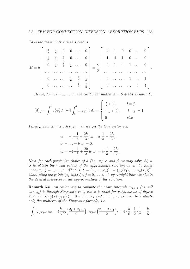
5.5. FEM FOR CONVECTION–DIFFUSION–ABSORPTION BVPS 133
Thus the mass matrix in this case is
M = h
23
16
0 0 . . . 0
16
23
16
0 . . . 0
0 16
23
16
. . . 0
. . . . . . . . . . . . . . . . . .
0 . . . . . . 16
23
16
0 . . . . . . . . . 16
23
=h
6
4 1 0 0 . . . 0
1 4 1 0 . . . 0
0 1 4 1 . . . 0
. . . . . . . . . . . . . . . . . .
0 . . . . . . 1 4 1
0 . . . . . . . . . 1 4
.
Hence, for i, j = 1, . . . , n, the coefficient matrix A = S + 4M is given by
[A]ij =
∫ 1
0
ϕ′iϕ
′j dx+ 4
∫ 1
0
ϕiϕj(x) dx =
2h+ 8h
3, i = j,
− 1h+ 2h
3, |i− j| = 1,
0 else.
Finally, with c0 = α och cn+1 = β, we get the load vector viz,
b1 = −(−1
h+
2h
3)c0 = α(
1
h− 2h
3),
b2 = . . . = bn−1 = 0,
bn = −(−1
h+
2h
3)cn+1 = β(
1
h− 2h
3).
Now, for each particular choice of h (i.e. n), α and β we may solve Aξ =b to obtain the nodal values of the approximate solution uh at the innernodes xj, j = 1, . . . , n. That is: ξ = (c1, . . . , cn)
T := (uh(x1), . . . , uh(xn))T .
Connecting the points (xj, uh(xj)), j = 0, . . . , n+1 by straight lines we obtainthe desired piecewise linear approximation of the solution.
Remark 5.5. An easier way to compute the above integrals mj,j+1 (as wellas mjj) is through Simpson’s rule, which is exact for polynomials of degree≤ 2. Since ϕj(x)ϕj+1(x) = 0 at x = xj and x = xj+1, we need to evaluateonly the midterm of the Simpson’s formula, i.e.
∫ 1
0
ϕjϕj+1 dx = 4h
6ϕj
(xj + xj+1
2
)· ϕj+1
(xj + xj+1
2
)· = 4 · h
6· 12· 12=h
6.

134 CHAPTER 5. TWO-POINT BOUNDARY VALUE PROBLEMS
For a uniform partition one may use ϕ0 = 1− x/h and ϕ1 = x/h on (0, h) :
∫ 1
0
ϕ0ϕ1 dx =
∫ h
0
(1− x
h)x
hdx =
[(1− x
h)x2
2h
]h0−
∫ h
0
(−1)
h· x
2
2hdx =
h
6.
Example 5.2. Below we consider a convection-diffusion problem:
−εu′′(x) + pu′(x) = r, 0 < x < 1; u(0) = 0, u′(1) = β 6= 0,
where ε and p are positive real numbers and r ∈ R. Here −εu′′ is the diffusionterm, pu′ corresponds to convection, and r is a given (here for simplicity aconstant) source (r > 0) or sink (r < 0). We would like to answer the samequestion as in the previous example. This time with c0 = u(0) = 0. Then,the test function at x = 0; ϕ0 will not be necessary. But since u(1) is notgiven, we shall need the test function at x = 1: ϕn+1. The function space forthe continuous solution: the trial function space, and the test function spaceare both the same:
V :=
w :
∫ 1
0
(w(x)2 + w′(x)2
)dx <∞, and w(0) = 0
.
We multiply the PDE by a test function v ∈ V and integrate over (0, 1).Then, integration by parts yields
−εu′(1)v(1) + εu′(0)v(0) + ε
∫ 1
0
u′v′dx+ p
∫ 1
0
u′vdx = r
∫ 1
0
v dx.
Hence, we end up with the variational formulation: find u ∈ V such that
(VF) ε
∫ 1
0
u′v′ dx+ p
∫ 1
0
u′v dx = r
∫ 1
0
v dx+ εβv(1), ∀v ∈ V.
The corresponding discrete test and trial function space is
V 0h := wh : wh is piecewise linear and continuous on T h, and wh(0) = 0.
Thus, the basis functions for V 0h are the hat-functions ϕj, j = 1, . . . , n + 1
(including the half-hat-function ϕn+1), and hence dim(V 0h ) = n+ 1.
Now the finite element formulation reads as follows: find uh ∈ V 0h such that
(FEM) ε
∫ 1
0
u′hv′ dx+ p
∫ 1
0
u′hv dx = r
∫ 1
0
v dx+ εβv(1), ∀v ∈ V 0h .

5.5. FEM FOR CONVECTION–DIFFUSION–ABSORPTION BVPS 135
ϕ0 ϕ2 ϕn+1ϕn
x0 = 0 x1 = h xn xn+1 = 1xj−1 xj xj+1
ϕj
Inserting the ansatz uh(x) =∑n+1
j=1 ξjϕj(x) into (FEM), and choosing v =ϕi(x), i = 1, . . . , n+ 1, we get
n+1∑
j=1
(ε
∫ 1
0
ϕ′j(x)ϕ
′i(x) dx+ p
∫ 1
0
ϕ′j(x)ϕi(x) dx
)ξj = r
∫ 1
0
ϕi(x) dx+ εβϕi(1),
In matrix form this corresponds to the linear system of equations Aξ = b withA = ε S + pC, where S is computed as Aunif and is the (n + 1) × (n + 1)-stiffness matrix with its last diagonal element, corresponding to the half-hat-function ϕn+1, i.e. as sn+1,n+1 =
∫ 1
0ϕ′n+1(x)ϕ
′n+1(x) dx = 1/h, and C is the
convection matrix with the elements
cij =
∫ 1
0
ϕ′j(x)ϕi(x) dx.
Hence we have, evidently,
S =1
h
2 −1 0 0 . . . 0
−1 2 −1 0 . . . 0
0 −1 2 −1 . . . 0
. . . . . . . . . . . . . . . . . .
0 . . . . . . −1 2 −1
0 . . . . . . . . . −1 1
.
To compute the entries for C, we note that like, S,M and S, also C is a

136 CHAPTER 5. TWO-POINT BOUNDARY VALUE PROBLEMS
tridiagonal matrix. But C is anti-symmetric. Its entries are
cij = 0, for |i− j| > 1
cii =∫ 1
0ϕi(x)ϕ
′i(x) dx = 0, for i = 1, . . . , n
cn+1,n+1 =∫ 1
0ϕn+1(x)ϕ
′n+1(x) dx = 1/2,
ci,i+1 =∫ 1
0ϕi(x)ϕ
′i+1(x) dx = 1/2, for i = 1, . . . , n
ci+1,i =∫ 1
0ϕi+1(x)ϕ
′i(x) dx = −1/2, for i = 1, . . . , n.
(5.5.5)
Finally, we have the entries bi of the load vector b as
b1 = . . . = bn = rh, bn+1 = rh/2 + εβ.
Thus,
C =1
2
0 1 0 0 . . . 0
−1 0 1 0 . . . 0
0 −1 0 1 . . . 0
. . . . . . . . . . . . . . . . . .
0 . . . . . . −1 0 1
0 . . . . . . . . . −1 1
, b = rh
1
1
1
·1
1/2
+ εβ
0
0
0
·0
1
.
Remark 5.6. Note that in the above example, since u(0) = 0, the half-hat-function ϕ0 is not needed. Whereas, if u(0) = a 6= 0, then the trial spaceshould contain ϕ0 in order to count for the non-zero contribution u(0) = a.Hence, V trial
h would have one-dimension more than the test function space,i.e.
V trialh = wh : wh is continuous, piecewise linear onTh, wh(0) = a
while the test function space remains as V 0h above. Further, since u(1) is not
given ( the data at x = 1 is u′(1) = β), both test and trial spaces shouldcontain the half-hat-function ϕn+1 at x = 1.
Remark 5.7. In the convection dominated case εp<< 1 this standard FEM
will not work. Spurious oscillations in the approximate solution will appear.The standard FEM has to be modified in this case.

5.6. EXERCISES 137
5.6 Exercises
Problem 5.1. Consider the two-point boundary value problem
−u′′ = f, 0 < x < 1; u(0) = u(1) = 0. (5.6.1)
Let V = v : ‖v‖+‖v′‖ <∞, v(0) = v(1) = 0, ‖ · ‖ denotes the L2-norm.
a. Use V to derive a variational formulation of (5.6.1).
b. Discuss why V is valid as a vector space of test functions.
c. Classify which of the following functions are admissible test functions
sin πx, x2, x ln x, ex − 1, x(1− x).
Problem 5.2. Assume that u(0) = u(1) = 0, and that u satisfies
∫ 1
0
u′v′ dx =
∫ 1
0
fv dx,
for all v ∈ V = v : ‖v‖+ ‖v′‖ <∞, v(0) = v(1) = 0.a. Show that u minimizes the functional
F (v) =1
2
∫ 1
0
(v′)2 dx−∫ 1
0
fv dx. (5.6.2)
Hint: F (v) = F (u+ w) = F (u) + . . . ≥ F (u).
b. Prove that the above minimization problem is equivalent to
−u′′ = f, 0 < x < 1; u(0) = u(1) = 0.
Problem 5.3. Consider the two-point boundary value problem
−u′′ = 1, 0 < x < 1; u(0) = u(1) = 0. (5.6.3)
Let Th : xj =j4, j = 0, 1, . . . , 4, denote a partition of the interval 0 < x < 1
into four subintervals of equal length h = 1/4 and let Vh be the correspondingspace of continuous piecewise linear functions vanishing at x = 0 and x = 1.
a. Compute a finite element approximation U ∈ Vh to (5.6.3).
b. Prove that U ∈ Vh is unique.

138 CHAPTER 5. TWO-POINT BOUNDARY VALUE PROBLEMS
Problem 5.4. Consider once again the two-point boundary value problem
−u′′ = f, 0 < x < 1; u(0) = u(1) = 0.
a. Prove that the finite element approximation U ∈ Vh to u satisfies
‖(u− U)′‖ ≤ ‖(u− v)′‖, ∀ v ∈ Vh.
b. Use this result to deduce that
‖(u− πhu)′‖ ≤ C‖hu′′‖, (5.6.4)
where C is a constant and πhu a piecewise linear interpolant to u.
Problem 5.5. Consider the two-point boundary value problem
−(au′)′ = f, x ∈ I := (0, 1),
u(0) = 0, a(1)u′(1) = g1,(5.6.5)
where a > 0 is a positive function and g1 is a constant.
a. Derive the variational formulation of (5.6.5).
b. Discuss how the boundary conditions are implemented.
Problem 5.6. Consider the two-point boundary value problem
−u′′ = 0, x ∈ I := (0, 1); u(0) = 0, u′(1) = 7. (5.6.6)
Divide the interval I into two subintervals of length h = 12and let Vh be
the corresponding space of continuous piecewise linear functions vanishing atx = 0.
a. Formulate a finite element method for (5.6.6).
b. Calculate by hand the finite element approximation U ∈ Vh to (5.6.6).
Study how the boundary condition at x = 1 is approximated.
Problem 5.7. Consider the two-point boundary value problem
−u′′ = 0, 0 < x < 1; u′(0) = 5, u(1) = 0. (5.6.7)
5.6. EXERCISES 139
Let Th : xj = jh, j = 0, 1, . . . , N, h = 1/N be a uniform partition of theinterval 0 < x < 1 into N subintervals and let Vh be the corresponding spaceof continuous piecewise linear functions.
a. Use Vh, with N = 3, and formulate a finite element method for (5.6.7).
b. Compute the finite element approximation U ∈ Vh assuming N = 3.
Problem 5.8. Consider the problem of finding a solution approximation to
−u′′ = 1, 0 < x < 1; u′(0) = u′(1) = 0. (5.6.8)
Let Th be a partition of the interval 0 < x < 1 into two subintervals of equallength h = 1
2and let Vh be the corresponding space of continuous piecewise
linear functions.
a. Find the exact solution to (5.6.8) by integrating twice.
b.Compute a finite element approximation U ∈ Vh to u if possible.
Problem 5.9. Consider the two-point boundary value problem
−((1 + x)u′)′ = 0, 0 < x < 1; u(0) = 0, u′(1) = 1. (5.6.9)
Divide the interval 0 < x < 1 into 3 subintervals of equal length h = 13and
let Vh be the corresponding space of continuous piecewise linear functionsvanishing at x = 0.
a. Use Vh to formulate a finite element method for (5.6.9).
b. Verify that the stiffness matrix A and the load vector b are given by
A =1
2
16 −9 0
−9 20 −11
0 −11 11
, b =
0
0
1
.
c. Show that A is symmetric tridiagonal, and positive definite.
d. Derive a simple way to compute the energy norm ‖U‖2E, defined by
‖U‖2E =
∫ 1
0
(1 + x)U ′(x)2 dx,
where U ∈ Vh is the finite element solution approximation.

140 CHAPTER 5. TWO-POINT BOUNDARY VALUE PROBLEMS
Problem 5.10. Consider the two-point boundary value problem
−u′′ = 0, 0 < x < 1; u(0) = 0, u′(1) = k(u(1)− 1). (5.6.10)
Let Th : 0 = x0 < x1 < x2 < x3 = 1, where x1 =13and x2 =
23be a partition
of the interval 0 ≤ x ≤ 1 and let Vh be the corresponding space of continuouspiecewise linear functions, which vanish at x = 0.
a. Compute a solution approximation U ∈ Vh to (5.6.10) assuming k = 1.
b. Discuss how the parameter k influence the boundary condition at x = 1.
In particular when k → ∞ and k → 0.
Problem 5.11. Consider the finite element method applied to
−u′′ = 0, 0 < x < 1; u(0) = α, u′(1) = β,
where α and β are given constants. Assume that the interval 0 ≤ x ≤ 1is divided into three subintervals of equal length h = 1/3 and that ϕj30 isa nodal basis of Vh, the corresponding space of continuous piecewise linearfunctions.
a. Verify that the ansatz
U(x) = αϕ0(x) + ξ1ϕ1(x) + ξ2ϕ2(x) + ξ3ϕ3(x),
yields the following system of equations
1
h
−1 2 −1 0
0 −1 2 −1
0 0 −1 1
α
ξ1
ξ2
ξ3
=
0
0
β
. (5.6.11)
b. If α = 2 and β = 3 show that (5.6.11) can be reduced to
1
h
2 −1 0
−1 2 −1
0 −1 1
ξ1
ξ2
ξ3
=
−2h−1
0
3
.
c. Solve the above system of equations to find U(x).

5.6. EXERCISES 141
Problem 5.12. Compute a finite element solution approximation to
−u′′ + u = 1; 0 ≤ x ≤ 1, u(0) = u(1) = 0, (5.6.12)
using the continuous piecewise linear ansatz U = ξ1ϕ1(x) + ξ2ϕ2(x) where
ϕ1(x) =
3x, 0 < x < 13
2− 3x, 13< x < 2
3,
0, 23< x < 1
ϕ2(x) =
0, 0 < x < 13
3x− 1, 13< x < 2
3.
3− 3x, 23< x < 1
Problem 5.13. Consider the following eigenvalue problem
−au′′ + bu = 0; 0 ≤ x ≤ 1, u(0) = u′(1) = 0, (5.6.13)
where a, b > 0 are constants. Let Th : 0 = x0 < x1 < . . . < xN = 1,be a non-uniform partition of the interval 0 ≤ x ≤ 1 into N intervals oflength hi = xi − xi−1, i = 1, 2, . . . , N and let Vh be the corresponding spaceof continuous piecewise linear functions. Compute the stiffness and massmatrices.
Problem 5.14. Show that the FEM with the mesh size h for the problem:
−u′′ = 1 0 < x < 1
u(0) = 1 u′(1) = 0,(5.6.14)
with
U(x) = 7ϕ0(x) + U1ϕ1(x) + . . .+ Umϕm(x). (5.6.15)
leads to the linear system of equations: A · U = b, where
A =1
h
−1 2 −1 0
0 −1 2 −1 . . .
. . . . . . . . . . . .
0 . . . 0 . . .
,
m× (m+ 1)
U =
7
U1
. . .
Um
,
(m+ 1)× 1
b =
h
. . .
h
h/2
,
m× 1

142 CHAPTER 5. TWO-POINT BOUNDARY VALUE PROBLEMS
. which is reduced to AU = b, with
A =1
h
2 −1 0 . . . 0
−1 2 −1 0 . . .
. . . . . . . . . . . . . . .
. . . 0 −1 2 −1
0 0 0 −1 2
, U =
U1
U2
. . .
Um
, b =
h+ 7h
h
. . .
h
h/2
.
Problem 5.15. Prove an a priori and an a posteriori error estimate for afinite element method (for example cG(1)) for the problem
−u′′ + αu = f, in I = (0, 1), u(0) = u(1) = 0,
where the coefficient α = α(x) is a bounded positive function on I, (0 ≤α(x) ≤ K, x ∈ I).
Problem 5.16. a) Formulate a cG(1) method for the problem
(a(x)u′(x))′ = 0, 0 < x < 1,
a(0)u′(0) = u0, u(1) = 0.
and give an a posteriori error estimate.
b) Let u0 = 3 and compute the approximate solution in a) for a uniformpartition of I = [0, 1] into 4 intervals and
a(x) =
1/4, x < 1/2,
1/2, x > 1/2.
c) Show that, with these special choices, the computed solution is equal to theexact one, i.e. the error is equal to 0.
Problem 5.17. Prove an a priori error estimate for the finite elementmethod for the problem
−u′′(x) + u′(x) = f(x), 0 < x < 1, u(0) = u(1) = 0.

5.6. EXERCISES 143
Problem 5.18. (a) Prove an a priori error estimate for the cG(1) approxi-mation of the boundary value problem
−u′′ + cu′ + u = f in I = (0, 1), u(0) = u(1) = 0,
where c ≥ 0 is constant.
(b) For which value of c is the a priori error estimate optimal?
Problem 5.19. Let U be the piecewise linear finite element approximationfor
−u′′(x) + 2xu′(x) + 2u(x) = f(x), x ∈ (0, 1), u(0) = u(1) = 0,
in a partition Th of the interval [0, 1]. Set e = u−U and derive a priori anda posteriori error estimates in the energy-norm:
||e||2E = ||e′||2 + ||e||2, where ||w||2 =∫ 1
0
w(x)2 dx.

144 CHAPTER 5. TWO-POINT BOUNDARY VALUE PROBLEMS

Chapter 6
Scalar Initial Value Problems
This chapter is devoted to finite element methods for time discretizations. Here,we shall consider problems depending on the time variable, only. The approxima-tion techniques developed in this chapter, combined with those of the previouschapter for boundary value problems, can be used for the numerical study ofinitial boundary value problems; such as, e.g. the heat and wave equations.
As a model problem we shall consider the classical example of populationdynamics described by the following ordinary differential equation (ODE)
(DE)
(IV)
u(t) + a(t)u(t) = f(t), 0 < t ≤ T,
u(0) = u0,(6.0.1)
where f(t) is the source term and u(t) =du
dt. The coefficient a(t) is a bounded
function. If a(t) ≥ 0 the problem (6.0.1) is called parabolic, while a(t) ≥ α > 0yields a dissipative problem, in the sense that, with increasing t, perturbationsof solutions to (6.0.1), e.g. introduced by numerical discretization, will decay.In general, in numerical approximations for (6.0.1), the error accumulates whenadvancing in time, i.e. the error of previous time steps adds up to the error ofthe present time step. The different types of error accumulation/perturbationgrowth are referred to as stability properties of the initial value problem.
145

146 CHAPTER 6. SCALAR INITIAL VALUE PROBLEMS
6.1 Solution formula and stability
Theorem 6.1. The solution of the problem (6.0.1) is given by
u(t) = u0 e−A(t) +
∫ t
0
e−(A(t)−A(s))f(s)ds, (6.1.1)
where A(t) =∫ t
0a(s)ds and eA(t) is the integrating factor.
Proof. Multiplying the (DE) by the integrating factor eA(t) we have
u(t)eA(t) + A(t)eA(t)u(t) = eA(t)f(t), (6.1.2)
where we used that a(t) = A(t). Equation (6.1.2) can be rewritten as
d
dt
(u(t)eA(t)
)= eA(t)f(t).
We denote the variable by s and integrate from 0 to t to get
∫ t
0
d
ds
(u(s)eA(s)
)ds =
∫ t
0
eA(s)f(s)ds,
i.e.
u(t)eA(t) − u(0)eA(0) =
∫ t
0
eA(s)f(s)ds.
Now since A(0) = 0 and u(0) = u0 we get the desired result
u(t) = u0e−A(t) +
∫ t
0
e−(A(t)−A(s))f(s)ds. (6.1.3)
This representation for u(t) is also referred to as the Variation of constantsformula.
Theorem 6.2 (Stability estimates). Using the solution formula, we can de-rive the following stability estimates:
(i) If a(t) ≥ α > 0, then |u(t)| ≤ e−αt|u0|+1
α(1− e−αt) max
0≤s≤t|f(s)|,

6.2. GALERKIN FINITE ELEMENT METHODS FOR IVP 147
(ii) If a(t) ≥ 0 (i.e. α = 0; the parabolic case), then
|u(t)| ≤ |u0|+∫ t
0
|f(s)|ds or |u(t)| ≤ |u0|+ ‖f‖L1(0,t). (6.1.4)
Proof. (i) For a(t) ≥ α > 0 we have that A(t) =
∫ t
0
a(s)ds is an increasing
function of t, A(t) ≥ αt and
A(t)− A(s) =
∫ t
0
a(r) dr −∫ s
0
a(r) dr =
∫ t
s
a(r) dr ≥ α(t− s). (6.1.5)
Thus e−A(t) ≤ e−αt and e−(A(t)−A(s)) ≤ e−α(t−s). Hence, using (6.1.3) we get
|u(t)| ≤ |u0|e−αt +
∫ t
0
e−α(t−s)|f(s)|ds, (6.1.6)
which yields
|u(t)| ≤ e−αt|u0|+ max0≤s≤t
|f(s)|[ 1αe−α(t−s)
]s=t
s=0, i.e.
|u(t)| ≤ e−αt|u0|+1
α(1− e−αt) max
0≤s≤t|f(s)|.
(ii) Let α = 0 in (6.1.6) (which is true also in this case), then |u(t)| ≤|u0|+
∫ t
0
|f(s)|ds, and the proof is complete.
Remark 6.1. (i) expresses that the effect of the initial data u0 decays expo-nentially with time, and that the effect of the source term f on the right handside does not depend on the length of the time interval, only on the maximumvalue of f , and on the value of α. In case (ii); the influence of u0 remainsbounded in time, and the integral of f indicates an accumulation in time.
6.2 Galerkin finite element methods for IVP
Recall that we refer to the set of functions where we seek the approximate so-lution as the trial space and the space of functions used for the orthogonalitycondition (multipliers), as the test space.

148 CHAPTER 6. SCALAR INITIAL VALUE PROBLEMS
The polynomial approximation procedure introduced in Chapter 2, along(2.1.21)-(2.2.6), for the initial value problem (2.1.1), and consequently alsofor (6.0.1), being over the whole time interval (0, T ) is referred as the globalGalerkin method. In this section, first we introduce two versions of the globalGalerkin method and then extend them to partitions of the interval (0, T )using piecewise polynomial test (multiplier) and trial (solution) functions.However, in most practical applications, if suffices to consider the followingtwo simple, low degree polynomial, approximation cases that are studied indetail in this chapter:• The continuous Galerkin method of degree 1; cG(1). In this case the trialfunctions are piecewise linear and continuous while the test functions arepiecewise constant and discontinuous, i.e. unlike the cG(1) for BVP, herethe trial and test functions belong to different polynomial spaces.
• The discontinuous Galerkin method of degree 0; dG(0). Here both the trialand test functions are chosen to be piecewise constant and discontinuous.
Below we introduce the global versions of the above two cases formulatedfor the whole time interval (0, T ) and then derive the local versions formulatedfor a partition of (0, T ).
6.2.1 The continuous Galerkin method
Recall the global Galerkin method of degree q; (2.2.1) for the initial valueproblem (6.0.1): find U ∈ Pq(0, T ), with U(0) = u0 such that
∫ T
0
(U + aU)vdt =
∫ T
0
fv dt, ∀v ∈ Pq(0, T ), with v(0) = 0. (6.2.1)
We formulate an alternative version for the above global method: FindU ∈ Pq(0, T ) with U(0) = u0 such that
∫ T
0
(U + aU)vdt =
∫ T
0
fvdt, ∀v ∈ Pq−1(0, T ), (6.2.2)
Note that in (6.2.1) we have that v ∈ spant, t2, . . . , tq, whereas in (6.2.2)v ∈ span1, t, t2, . . . , tq−1. Hence, the difference between these two formula-tion lies in the choice of their test function spaces. We shall focus on (6.2.2),

6.2. GALERKIN FINITE ELEMENT METHODS FOR IVP 149
due to the fact that, actually, this method yields a more accurate approxi-mation of degree q than the original method (6.2.1). The following exampleillustrates this phenomenon
Example 6.1. Consider the IVP
u(t) + u(t) = 0, 0 ≤ t ≤ 1,
u(0) = 1.(6.2.3)
The exact solution is given by u(t) = e−t. The continuous piecewise linearapproximation, with the ansatz U(t) = 1 + ξ1t in,
∫ 1
0
(U(t) + U(t))v(t) dt = 0, (6.2.4)
and v(t) = t (i.e. (6.2.1)) yields
∫ 1
0
(ξ1 + 1 + ξ1t)t dt = 0 =⇒[(ξ1 + 1)
t2
2+ ξ1
t3
3
]10= 0 =⇒ ξ= − 3/5.
Hence in this case the approximate solution, that we denote by U1 is givenby U1(t) = 1− (3/5)t. Whereas (6.2.2) for this problem means v(t) = 1 andgives
∫ 1
0
(ξ1 + 1 + ξ1t) dt = 0 =⇒[(ξ1 + 1)t+ ξ1
t2
2
]10= 0 =⇒ ξ= − 2/3.
In this case the approximate solution that we denote by U2 is given as U2(t) =1− (2/3)t. As we can see in the figure below U2 is a better approximation fore−t than U1.
Before generalizing (6.2.2) to approximation by piecewise polynomials ofdegree q, which is the cG(q) method, we consider an example.
Example 6.2. Consider (6.2.2) with q = 1, then we may choose v ≡ 1, thus
∫ T
0
(U + aU)vdt =
∫ T
0
(U + aU)dt = U(T )− U(0) +
∫ T
0
aU(t)dt (6.2.5)
But U(t) being a linear function on [0, T ] is given by
U(t) = U(0)T − t
T+ U(T )
t
T. (6.2.6)

150 CHAPTER 6. SCALAR INITIAL VALUE PROBLEMS
1
1
U1(t)
U2(t)
t
u(t) = e−t
Figure 6.1: Two continuous linear Galerkin approximations of e−t.
Inserting into (6.2.5) we get
U(T )− U(0) +
∫ T
0
a(U(0)
T − t
T+ U(T )
t
T
)dt =
∫ T
0
f dt, (6.2.7)
which gives an equation for the unknown quantity U(T ). Thus, using (6.2.6)with a given U(0), we get the linear approximation U(t) for all t ∈ [0, T ]. Be-low we generalize this example to piecewise linear approximation and demon-strate the iteration procedure for the cG(1) scheme.
The cG(1) AlgorithmFor a partition Tk of the interval [0, T ] into subintervals Ik = (tk−1, tk], k =1, 2, . . . , n, we perform the following steps:
(1) Given U(0) = U0 = u0 and a source term f , apply (6.2.7) to the firstsubinterval (0, t1] and compute U(t1). Then, using (6.2.6) one getsU(t), ∀t ∈ [0, t1].
(2) Assume that we have computed Uk−1 := U(tk−1). Hence, Uk−1 andf are now considered as data. Now we consider the problem on thesubintervals Ik = (tk−1, tk], and compute the unknown Uk := U(tk)from the local version of (6.2.7),
Uk − Uk−1 +
∫ tk
tk−1
a( tk − t
tk − tk−1
Uk−1 +t− tk−1
tk − tk−1
Uk
)dt =
∫ tk
tk−1
fdt.

6.2. GALERKIN FINITE ELEMENT METHODS FOR IVP 151
(3) Having both Uk−1 and Uk, by linearity, we get U(t) for t ∈ Ik. To get thecontinuous piecewise linear approximation in the whole interval [0, tN ],step (2) is performed in successive subintervals Ik, k = 2, . . . , N .
The cG(q) methodThe Global continuous Galerkin method of degree q formulated on a partitionTk, 0 = t0 < t1 < . . . < tN = T of the interval (0, T ), is referred to as the
cG(q) method and reads as follows: find U(t) ∈ V(q)k , such that U(0) = u0,
and ∫ tN
0
(U + aU)wdt =
∫ tN
0
fwdt, ∀w ∈ W(q−1)k , (6.2.8)
where
V(q)k = v : v continuous, piecewise polynomials of degree ≤ q on Tk,
W(q−1)k = w : w discontinuous, piecewise polynomials of degree ≤ q−1 on Tk.
So, the difference between the global continuous Galerkin method and cG(q)is that now we have piecewise polynomials on a partition of [0, T ] rather thanglobal polynomials in the whole interval [0, T ].
6.2.2 The discontinuous Galerkin method
We start presenting the global discontinuous Galerkin method of degree q:find U(t) ∈ Pq(0, T ) such that
∫ T
0
(U + aU)vdt+ β(U(0)− u(0))v(0) =
∫ T
0
fvdt, ∀v ∈ Pq(0, T ), (6.2.9)
where β is a coefficient that weights the relative importance of the resid-ual error for the initial value U(0) − u(0), against the conventional residualR(U) := U + aU − f of the differential equation. This approach gives upthe requirement that U(t) satisfies the initial condition. Instead, the initialcondition is imposed in a variational sense by the term (U(0)−u(0))v(0). Asin the cG(q) case, to derive the discontinuous Galerkin method of degree q:the dG(q) scheme, the above strategy can be formulated for the subintervalsin a partition Th. To this end, we recall the notation for the right/left limits:v±n = lim
s→0+v(tn ± s) and the corresponding jump term [vn] = v+n − v−n at

152 CHAPTER 6. SCALAR INITIAL VALUE PROBLEMS
tn−1 tn tn+1t
kn
v−n
[vn]
v+n
•
•
Figure 6.2: The jump [vn] and the right and left limits v±n
time level t = tn. Then, the dG(q) method (with β ≡ 1) for (6.0.1) reads asfollows: for n = 1, . . . , N ; find U(t) ∈ Pq(tn−1, tn) such that
∫ tn
tn−1
(U + aU)vdt+ U+n−1v
+n−1 =
∫ tn
tn−1
fvdt+ U−n−1v
+n−1, ∀v ∈ Pq(tn−1, tn).
(6.2.10)
Example 6.3 (dG(0)). Let q = 0, then v is constant generated by the singlebasis function: v ≡ 1. Further, we have U(t) = Un = U+
n−1 = U−n on
In = (tn−1, tn], and U ≡ 0. Thus, for q = 0 (6.2.10) yields the followingdG(0) formulation: for n = 1, . . . , N ; find piecewise constants Un such that
∫ tn
tn−1
aUndt+ Un =
∫ tn
tn−1
fdt+ Un−1. (6.2.11)
Summing over n in (6.2.10), we get the following general dG(q) formulation:
Find U(t) ∈ W(q)k , with U−
0 = u0 such that
N∑
n=1
∫ tn
tn−1
(U + aU)wdt+N∑
n=1
[Un−1]w+n−1 =
∫ tN
0
fwdt, ∀w ∈ W(q)k . (6.2.12)
Remark 6.2. One can show that (see Johnson et al [20]) cG(1) convergesfaster than dG(0), whereas dG(0) has better stability properties than cG(1):More specifically, in the parabolic case when a > 0 is constant and (f ≡ 0)

6.3. A POSTERIORI ERROR ESTIMATES 153
we can easily verify that (see Exercise 6.10 at the end of this chapter) thedG(0) solution Un corresponds to the Backward Euler scheme
Un =( 1
1 + ak
)n
u0,
and the cG(1) solution Un is given by the Crank-Nicolson scheme:
Un =(1− 1
2ak
1 + 12ak
)n
u0,
where k is the constant time step.
6.3 A posteriori error estimates
In this section we derive a posteriori error estimates for the most consideredGalerkin approaches for time discretization, namely the cG(1) and dG(0)methods. These estimates can be extended to the general cG(q) and dG(q)methods. The details are, however, “much too” involved. Some lower degreepolynomial case (e.g. cG(2)) are left as exercise.
6.3.1 A posteriori error estimate for cG(1)
Recall the initial value problem (6.0.1) of finding the function u such that
u(t) + a(t)u(t) = f(t), ∀t ∈ (0, T ], u(0) = u0. (6.3.1)
A general variational form reads as: find u such that
∫ T
0
(u+ au)vdt =
∫ T
0
fvdt, for all test functions v.
Integrating by parts we get the equivalent equation
u(T )v(T )− u(0)v(0) +
∫ T
0
u(t)(−v(t) + av(t))dt =
∫ T
0
fvdt. (6.3.2)
If we now choose the test function v(t) to be the solution of the dual problem:
−v(t) + av(t) = 0, for t ∈ (0, T ), (6.3.3)

154 CHAPTER 6. SCALAR INITIAL VALUE PROBLEMS
then (6.3.2) is simplified to
u(T )v(T ) = u(0)v(0) +
∫ T
0
fvdt, ∀v(t). (6.3.4)
In other words, choosing v to be the solution of the dual problem (6.3.3), wemay get the final value u(T ) of the solution directly coupled to the initialvalue u(0) and the data f . This type of representation will be crucial in thea posteriori error analysis, e.g. in the proof of the next theorem. Let us statethe dual problem explicitly:
The dual problemThe dual problem for (6.3.1) is formulated as follows: find ϕ(t) such that
−ϕ(t) + a(t)ϕ(t) = 0, tN > t ≥ 0,
ϕ(tN) = eN , where eN = uN − UN = u(tN)− U(tN).(6.3.5)
u, ϕ
t
u(t) problem
ϕ(t) problem
•T
Figure 6.3: Time directions in forward and dual solutions
Note that (6.3.5) runs backward in time starting at time tN = T .
Theorem 6.3 (A posteriori error estimate for cG(1)). For N = 1, 2, . . ., thecG(1) solution U(t) satisfies
|eN | ≤ S(tN) · maxt∈[0,tN ]
|k r(U)|, (6.3.6)
where k(t) is the time step function: k(t) = kn = |In| for t ∈ In = (tn−1, tn],and r(U) = U + aU − f is the residual error for U . Further S(tN), specifiedbelow, is the stability factor satisfying the quantitative bound
S(tN) :=
∫ tN0
|ϕ|dt|eN |
≤
eλ tN , if |a(t)| ≤ λ, for 0 ≤ t ≤ tN ,
1, if a(t) ≥ 0, for 0 ≤ t ≤ tN .
(6.3.7)

6.3. A POSTERIORI ERROR ESTIMATES 155
Proof. Let e(t) = u(t)− U(t). Using the dual problem −ϕ(t) + a(t)ϕ(t) = 0we may write
e2N = e2N + 0 = e2N +
∫ tN
0
e(−ϕ+ aϕ) dt, (6.3.8)
and by integration by parts we get
∫ tN
0
e(−ϕ+ aϕ)dt = [−e(t)ϕ(t)]tNt=0 +
∫ tN
0
eϕ dt+
∫ tN
0
eaϕ dt
= −e(tN)ϕ(tN) +∫ tN
0
(e+ ae)ϕdt = −e2N +
∫ tN
0
(e+ ae)ϕdt,
where we used that e(0) = 0 and ϕ(tN) = eN when evaluating the boundaryterms. Note that
e(t) + a(t)e(t) = u(t)− U(t) + a(t)u(t)− a(t)U(t)
= f(t)− U(t)− a(t)U(t) := −r(U),(6.3.9)
where we used that f(t) = u(t)+a(t)u(t) and the residual r(U) := U+aU−f .Consequently, we get the following error representation formula:
e2N = −∫ tN
0
r(U(t))ϕ(t)dt. (6.3.10)
To proceed we use the L2-projection πkϕ = 1kn
∫Inϕ(s)ds of ϕ onto the space
of piecewise constant polynomials W(0)k and write
e2N = −∫ tN
0
r(U)(ϕ(t)− πkϕ(t))dt−∫ tN
0
r(U)πkϕ(t)dt. (6.3.11)
Now, by the cG(1) method (6.2.8),
∫ tN
0
(U + aU)v dt =
∫ tN
0
fv dt, ∀v ∈ W(0)k , (6.3.12)
where W(0)k is the space of discontinuous, piecewise constant test functions.
This gives the orthogonality relation, r(U) ⊥ v, ∀v ∈ W(0)k , and implies that
∫ tN
0
r(U)πkϕ(t)dt = 0, (6.3.13)

156 CHAPTER 6. SCALAR INITIAL VALUE PROBLEMS
since πkϕ ∈ W(0)k . Thus, the final error representation formula reads
e2N = −∫ tN
0
r(U)(ϕ(t)− πkϕ(t))dt. (6.3.14)
Next, we shall need the L2-projection error estimate (proved as the interpo-lation error estimate) for the function ϕ in the interval In, with |In| = kn:
∫ tN
0
|ϕ− πkϕ|dt ≤N∑
n=1
kn
∫
In
|ϕ|dt. (6.3.15)
To show (6.3.15) let ϕ = 1kn
∫Inϕ(s)ds be the mean value of ϕ over In, then
∫
In
|ϕ− πkϕ|dt =∫
In
|ϕ− ϕ|dt
=
∫
In
|ϕ(t)− ϕ(ξ)|dt =∫
In
|∫ t
ξ
ϕ(s) ds|dt
≤∫
In
|∫
In
ϕ(s) ds|dt = kn ·∫
In
|ϕ|dt,
where we have used the mean value theorem for integrals, with ξ ∈ In.Summing over n, yields the global estimate
∫ tN
0
|ϕ− πkϕ|dt =N∑
n=1
∫
In
|ϕ− πkϕ|dt ≤N∑
n=1
kn
∫
In
|ϕ|dt. (6.3.16)
Now let |v|J := maxt∈J
|v(t)|, then using (6.3.16) and the final form of the error
representation formula (6.3.14) we have that
|eN |2 ≤N∑
n=1
(|r(U)|Inkn
∫
In
|ϕ|dt)≤ max
1≤n≤N(kn|r(U)|In)
∫ tN
0
|ϕ|dt.
Since, by the definition of S(tN),∫ tN0
|ϕ|dt = |eN | · S(tN), we finally get
|eN |2 ≤ |eN |S(tN) maxt∈[0,tN ]
(|kr(U)|). (6.3.17)
This completes the proof of the first assertion of the theorem.

6.3. A POSTERIORI ERROR ESTIMATES 157
To prove the second assertion, we transform the dual problem (6.3.5) to aforward problem, using the change of variables, viz s = tN − t, (t = tN − s).Thus for ψ(s) := ϕ(tN − s), using the chain rule we get
dψ
ds=dϕ
dt· dtds
= −ϕ(tN − s). (6.3.18)
The dual problem (6.3.5) is now reformulated as: find ϕ(t) such that
−ϕ(tN − s) + a(tN − s)ϕ(tN − s) = 0. (6.3.19)
The corresponding forward problem for ψ reads as follows: find ψ(s) suchthat
dψ(s)
ds+ a(tN − s)ψ(s) = 0, 0 < s ≤ tN
ψ(0) = ϕ(tN) = eN , eN = uN − UN = u(tN)− U(tN).
By the solution formula (6.1.1) this problem has the solution ψ(s) given by
ψ(s) = ψ(0) · e−∫ s
0a(tN−u) du = [tN − u = v, −du = dv]
= eN · e∫ tN−s
tNa(v) dv = eN · eA(tN−s)−A(tN ).
Inserting back into the relation ϕ(t) = ψ(s), with t = tN − s, we end up with
ϕ(t) = eNeA(t)−A(tN ), and ϕ(t) = eNa(t)e
A(t)−A(tN ). (6.3.20)
To estimate S(tN) we note that for a(t) ≥ 0, the second relation in (6.3.20)yields
∫ tN
0
|ϕ(t)|dt = |eN |∫ tN
0
a(t)eA(t)−A(tN )dt = |eN |[eA(t)−A(tN )]tNt=0
= |eN |(1− eA(0)−A(tN )
)= |eN |
(1− e−A(tN )
)≤ |eN |,
which gives S(tN) =
∫ tN0
|ϕ(t)|dt|eN |
≤ 1.
As for the case |a(t)| ≤ λ, we use again (6.3.20): ϕ(t) = a(t)eNeA(t)−A(tN )
and write
|ϕ(t)| ≤ λ|eN |eA(t)−A(tN ) = λ|eN |e∫ t
tNa(s)ds ≤ λ|eN |eλ(tN−t). (6.3.21)

158 CHAPTER 6. SCALAR INITIAL VALUE PROBLEMS
Integrating over (0, tN) we get
∫ tN
0
|ϕ(t)|dt ≤ |eN |∫ tN
0
λeλ(tN−t)dt = |eN |[− eλ(tN−t)
]tN0
= |eN |(−1 + eλtN ),
which gives that S(tN) ≤ (−1+ eλtN ) ≤ eλtN , and completes the proof of thesecond assertion.
The convergence rate in (6.3.6) appears to be of orderO(k), but is actuallyof order O(k2) since |r(U)| ≤ Ck if f is a smooth function. To prove theconvergence of order O(k2), we use some further orthogonality observationsin the following theorem.
Theorem 6.4 ( Convergence order O(k2)). For N = 1, 2, . . ., and with SN
as in the previous theorem, the error for the cG(1) solution U(t) satisfies
|eN | ≤ S(tN) maxt∈[0,tN ]
∣∣∣k2d
dt(aU − f)
∣∣∣. (6.3.22)
W(0)k
πkg(t)
g(t) g(t)− πkg(t)
Figure 6.4: Orthogonality: (g(t)− πkg(t)) ⊥ (constants) ∀g(t).
Proof. Let πkg be the L2-projection of g onto the space W(0)k of piecewise
constant polynomials. Then, by the orthogonality relation(g(t)−πkg(t)
)⊥
(constants) ∀g(t), since U(t) is constant on each subinterval In we have that∫ tN0U(ϕ− πkϕ)dt = 0. Thus using the error representation formula (6.3.14),

6.3. A POSTERIORI ERROR ESTIMATES 159
we may write
e2N = −∫ tN
0
r(U)(ϕ(t)− πkϕ(t)
)dt =
∫ tN
0
(f − aU − U)(ϕ− πkϕ)dt
=
∫ tN
0
(f − aU)(ϕ− πkϕ)dt−∫ tN
0
U(ϕ− πkϕ)dt
= −∫ tN
0
(aU − f)(ϕ− πkϕ)dt.
Similarly, using the fact that πk(aU − f) is constant on each subinterval In,we have ∫ tN
0
πk(aU − f)(ϕ− πkϕ)dt = 0. (6.3.23)
Consequently we can write
e2N = −∫ tN
0
((aU − f)− πk(aU − f)
)(ϕ− πkϕ)dt. (6.3.24)
(compare (6.3.24) with (6.3.14)). To proceed recall that for t ∈ In:
g(t)− πkg(t) = g(t)− g(t) = g(t)− g(ξ) =
∫ t
ξ
g(s) ds,
where g is the mean value of g over In, ξ ∈ In and we have used the meanvalue theorem for the integrals. This implies
|g(t)− πkg(t)| ≤∫
In
|g(t)| dt ≤ maxt∈In
|g(t)| · kn, (6.3.25)
Now we apply (6.3.6) with r(U) replaced by (aU − f)− πk(aU − f), (6.3.25)with g := aU − f , and the L2-projection error estimate to get
|eN | ≤ S(tN)∣∣∣k|(aU − f)− πk(aU − f)|
∣∣∣[0,tN ]
≤ S(tN)∣∣∣k2
d
dt(aU − f)
∣∣[0,tN ]
,
which is the desired result.
Remark 6.3. Note that the estimate (6.3.22) is less practical than the es-timate (6.3.6) in the sense that: it requires the cumbersome procedure ofcomputing the time derivative of the residual.

160 CHAPTER 6. SCALAR INITIAL VALUE PROBLEMS
6.3.2 A posteriori error estimate for dG(0)
We shall now derive an a posteriori error estimate for the dG(0) method. Inthis case, the residual contains jump discontinuities.
Theorem 6.5. For N = 1, 2, . . ., the dG(0) solution U(t) satisfies
|u(tN)− UN | ≤ S(tN)|kR(U)|[0,tN ], UN = U(tN) (6.3.26)
where
R(U) = |f − aU |+ |Un − Un−1|kn
for tn−1 < t ≤ tn. (6.3.27)
Proof. The proof is similar to that of the cG(1) approach of Theorem 6.3,but we have to take the discontinuities of U(t) at the time nodes tj intoaccount. Below we shall first demonstrate how to rearrange the contributionfrom these jumps, and in this way derive a corresponding error representationformula. To this end, recalling the dual problem −ϕ(t) + a(t)ϕ(t) = 0, withϕ(tN) = eN , we may write, using integration by parts on each subinterval
e2N = e2N +N∑
n=1
∫ tn
tn−1
e(−ϕ(t) + a(t)ϕ(t))dt
= e2N +N∑
n=1
(∫ tn
tn−1
(e+ ae)ϕ(t)dt− [eϕ]tntn−1
)
= e2N +N∑
n=1
∫ tn
tn−1
(f − aU)ϕdt−N∑
n=1
[eϕ]tntn−1,
(6.3.28)
where in the last step we have used e+ae = u− U +au−aU = f −aU sinceU = 0 on each subinterval (where U is constant). For a given function g weuse the notation g(t−n ) = g−n and g(t+n−1) = g+n−1, and rewrite the last sum as
N∑
n=1
[eϕ]tntn−1=
N∑
n=1
(e(t−n )ϕ(t
−n )− e(t+n−1)ϕ(t
+n−1)
)
=N∑
n=1
(e−nϕ−n − e+n−1ϕ
+n−1) = (e−1 ϕ
−1 − e+0 ϕ
+0 ) + (e−2 ϕ
−2 − e+1 ϕ
+1 )
+ . . .+ (e−N−1ϕ−N−1 − e+N−2ϕ
+N−2) + (e−Nϕ
−N − e+N−1ϕ
+N−1).

6.3. A POSTERIORI ERROR ESTIMATES 161
We use the identity ϕ−i = (ϕ−
i − ϕ+i + ϕ+
i ), i = 1, . . . N − 1, and rewrite thecontribution from the jumps as
−N∑
n=1
[eϕ]tntn−1= −e−Nϕ−
N + e+0 ϕ+0 − e−1 (ϕ
−1 − ϕ+
1 + ϕ+1 ) + e+1 ϕ
+1
− e−2 (ϕ−2 − ϕ+
2 + ϕ+2 ) + e+2 ϕ
+2 − . . .
− e−N−1(ϕ−N−1 − ϕ+
N−1 + ϕ+N−1) + e+N−1ϕ
+N−1.
Here the general i-th term is written as
− e−i (ϕ−i − ϕ+
i + ϕ+i ) + e+i ϕ
+i = −e−i ϕ−
i + e−i ϕ+i − e−i ϕ
+i + e+i ϕ
+i
= e−i (ϕ+i − ϕ−
i ) + ϕ+i (e
+i − e−i ) = e−i [ϕi] + ϕ+
i [ei],
with [g] = g+ − g− representing the jump. Hence we have
−N∑
n=1
[eϕ]tntn−1= −e2N + e+0 ϕ
+0 +
N−1∑
n=1
[en]ϕ+n +
N−1∑
n=1
e−n [ϕn]. (6.3.29)
Inserting into (6.3.28) and using the fact that ϕ and u are smooth, i.e. [ϕn] =[un] = 0 and [en] = [−Un], we get the following error representation formula
e2N = e2N +N∑
n=1
∫ tn
tn−1
(f − aU)ϕdt− e2N + e+0 ϕ+0 +
N−1∑
n=1
[en]ϕ+n +
N−1∑
n=1
[ϕn]e−n
= e+0 ϕ+0 +
N∑
n=1
∫ tn
tn−1
(f − aU)ϕdt−N−1∑
n=1
[Un]ϕ+n
=N∑
n=1
(∫ tn
tn−1
(f − aU)ϕdt− [Un−1]ϕ+n−1
)
=N∑
n=1
∫ tn
tn−1
(f − aU)(ϕ− πkϕ) dt− [Un−1](ϕ− πkϕ)+n−1,
where we have used e+0 = u+0 − U+0 = u0 − U+
0 = U−0 − U+
0 = −[U0], and inthe last step, once again, we use definition (6.2.12) of dG(q) with q = 0 and
the L2 projection w = πkϕ ∈ W(0)k (space of piecewise constants) of ϕ. The
remaining part is not substantially different from the proof of Theorem 6.3,and is therefore omitted.

162 CHAPTER 6. SCALAR INITIAL VALUE PROBLEMS
6.3.3 Adaptivity for dG(0)
To guarantee a desired local bound for the error of the dG(0) approximationU(t), such as
|en| = |u(tn)− U(tn)| ≤ TOL, (6.3.30)
where TOL is a given tolerance, we seek to determine the time step kn =tn − tn−1 so that, using (6.3.26), locally, we have
S(tN)maxt∈In
|knR(U)| ≤ TOL, n = 1, 2, . . . , N. (6.3.31)
Adaptivite algorithm
(i) Compute Un from Un−1 using a predicted step kn, and the relation
∫ tn
tn−1
aUndt+ Un =
∫ tn
tn−1
fdt+ Un−1. (6.3.32)
(ii) Compute |kR(U)|In := maxt∈In
|knR(U)|, whereR(U) = |f−aU |+ |Un−Un−1|kn
in In, and follow the chart:
Is (6.3.31) validfor this choice of kn?
yes−→
Accept the solution Un
and go to the next time stepx noy
Recompute (6.3.32)with a smaller kn

6.4. A PRIORI ERROR ANALYSIS 163
6.4 A priori error analysis
In this section we shall derive a priori error estimates for the dG(0) method.For simplicity, first we assume that a is a constant, and then we study theparabolic case a(t) ≥ 0, where we perform a refined analysis. The corre-sponding a priori error estimate for the cG(1) method is obtained similarly.The weaker stability properties of cG(1), however, do not allow a refinedanalysis in the parabolic case.
6.4.1 A priori error estimates for the dG(0) method
The dG(0) method for u+ au = f , with a constant a, is formulated as: findU = U(t), t ∈ In, such that
∫ tn
tn−1
Udt+ a
∫ tn
tn−1
Udt =
∫
In
fdt, n = 1, 2, . . . (6.4.1)
Note that U(t) = Un is constant for t ∈ In. Let Un = U(tn), Un−1 = U(tn−1)and kn = tn − tn−1, then
∫ tn
tn−1
Udt+ a
∫ tn
tn−1
Udt = Un − Un−1 + aknUn.
Hence with a given initial data u(0) = u0, the equation (6.4.1) is written as
Un − Un−1 + aknUn =
∫
In
fdt. n = 1, 2, . . . U0 = u0. (6.4.2)
For the exact solution u(t) of u+ au = f , the same procedure yields
u(tn)− u(tn−1) + aknu(tn) =
∫
In
fdt+ aknu(tn)− a
∫ tn
tn−1
u(t)dt, (6.4.3)
where we have moved the term a∫ tntn−1
u(t)dt to the right hand side and added
aknu(tn) to both sides. Thus from (6.4.2) and (6.4.3) we have that, denotingun = u(tn),
(1 + kna)Un = Un−1 +
∫
In
fdt,
(1 + kna)un = un−1 +
∫
In
fdt+ aknun − a
∫ tn
tn−1
u(t)dt.
(6.4.4)

164 CHAPTER 6. SCALAR INITIAL VALUE PROBLEMS
Now let en = un − Un, then en−1 = un−1 − Un−1, and subtracting the firstequation in (6.4.4) from the second one yields
en = (1+kna)−1(en−1+ρn), where ρn := aknun−a
∫ tn
tn−1
u(t)dt. (6.4.5)
Thus, to estimate en we use an iteration procedure combined with an estimatefor ρn.
Lemma 6.1. We have that
|ρn| ≤1
2|a|k2n max
In|u(t)| (6.4.6)
Proof. Evidently,
|ρn| =∣∣∣aknun − a
∫ tn
tn−1
u(t) dt∣∣∣ = |a|kn
∣∣∣un −1
kn
∫
In
u(t) dt∣∣∣
= |a|∣∣∣∫ tn
tn−1
(un − u(t)) dt∣∣∣ = |a|
∣∣∣∫ tn
tn−1
∫ tn
t
u(s) ds dt∣∣∣
≤ |a|maxIn
|u(t)| ·∫ tn
tn−1
(tn − t) dt =1
2|a|k2n ·max
In|u(t)|.
(6.4.7)
To simplify the estimate for en we split, and gather, the proof of technicaldetails in the following lemma:
Lemma 6.2. For kn|a| ≤ 1/2, and n ≥ 1 we have that
(i) (1− kn|a|)−1 ≤ e2kn|a|,
(ii) |eN | ≤1
2
N∑
n=1
(e2|a|τn |a|kn)(
max1≤n≤N
kn|u|In), τn = tN − tn−1.
(iii)N∑
n=1
e2|a|τn |a|kn ≤ e
∫ tN
0
|a|e2|a|τdτ .
We postpone the proof of this lemma and first show that using (i)− (iii)we can prove the following a priori error estimate.

6.4. A PRIORI ERROR ANALYSIS 165
Theorem 6.6. If kn|a| ≤ 12, n ≥ 1 then the error for the dG(0) approxima-
tion U satisfies
|u(tN)− U(tN)| = |eN | ≤e
4
(e2|a|tN − 1
)max
1≤n≤Nkn|u(t)|In . (6.4.8)
Proof. Using estimates (ii) and (iii) of the above lemma we have that
|eN | ≤1
2
N∑
n=1
(e2|a|τn |a|kn) max1≤n≤N
kn|u|In ≤ 1
2
(e
∫ tN
0
|a|e2|a|τdτ)
max1≤n≤N
kn|u|In
=1
2e[e2|a|τ
2
]tN0
max1≤n≤N
kn|u(t)|In =e
4
(e2|a|tN − 1
)max
1≤n≤Nkn|u(t)|In ,
and the proof is complete.
Note that the stability factore
4
(e2|a|tN−1
)grows exponentially depending
on |a| and tN , hence this result may not be satisfactory at all. We deal withthis question below in the parabolic case a(t) ≥ 0.
Remark 6.4. The a priori error estimate for the cG(1) method is similarto that of Theorem 6.6, with kn|u| replaced by k2n|u|.
We now return to the proof of our technical results (i)− (iii):
Proof of Lemma 6.3. (i) For 0 < x := kn|a| ≤ 1/2, we have that 1/2 ≤1−x < 1 implies 0 ≤ 1−2x < 1. We may multiply both sides of
1
1− x< e2x
(which is the result we want to prove) by 1 − x ≥ 1/2 > 0 to obtain theequivalent relation
f(x) := (1− x)e2x − 1 > 0. (6.4.9)
Note that since f(0) = 0 and f ′(x) = (1 − 2x)e2x ≥ 0 (equality for x = 12),
thus (6.4.9), and hence the relation (i) is valid.To prove (ii) we recall that en = (1+kna)
−1(en−1+ρn). To deal with the
factor (1+kna)−1 we use kn|a| ≤
1
2, then by (i) (1+kna)
−1 ≤ (1−kn|a|)−1 ≤e2kn|a|, n ≥ 1. Thus
|eN | ≤1
1− kN |a||eN−1|+
1
1− kN |a||ρN | ≤ |eN−1|e2kN |a| + |ρN |e2kN |a|.
(6.4.10)

166 CHAPTER 6. SCALAR INITIAL VALUE PROBLEMS
Relabeling, N to N − 1,
|eN−1| ≤ |eN−2|e2kN−1|a| + |ρN−1|e2kN−1|a| = e2kN−1|a|(|eN−2|+ |ρN−1|
),
and inserting into (6.4.10) yields
|eN | ≤ e2kN |a|e2kN−1|a|(|eN−2|+ |ρN−1|
)+ |ρN |e2kN |a|. (6.4.11)
Similarly we have |eN−2| ≤ e2kN−2|a|(|eN−3|+ |ρN−2|
). Now iterating (6.4.11)
and using the fact that e0 = 0 we get,
|eN | ≤e2kN |a|e2kN−1|a|e2kN−2|a||eN−3|+ e2kN |a|e2kN−1|a|e2kN−2|a||ρN−2|+ e2kN |a|e2kN−1|a||ρN−1|+ |ρN |e2kN |a| ≤ · · · ≤
≤e2|a|∑N
n=1kn |e0|+
N∑
n=1
e2|a|∑N
m=n km |ρn| =N∑
n=1
e2|a|∑N
m=n km |ρn|.
Recalling (6.4.6): |ρn| ≤1
2|a|k2n max
In|u(t)|, we have the error estimate
|eN | ≤( N∑
n=1
e2|a|∑N
m=n km)12|a|k2n max
In|u(t)|. (6.4.12)
Note that
N∑
m=n
km = (tn−tn−1)+(tn+1−tn)+(tn+2−tn+1)+. . .+(tN−tN−1) = tN−tn−1.
Hence, since τn = tN − tn−1, we have shown assertion (ii), i.e.
|eN | ≤N∑
n=1
e2|a|(tN−tn−1)1
2|a|k2n max
In|u(t)| ≤ 1
2
N∑
n=1
(e2|a|τn |a|kn)(
max1≤n≤N
kn|u|In).
(iii) To prove this part we note that
τn = tN − tn−1 = (tN − tn) + (tn − tn−1) = τn+1 + kn, (6.4.13)

6.5. THE PARABOLIC CASE (A(T ) ≥ 0) 167
and since |a|kn ≤ 1/2 we have 2|a|τn = 2|a|τn+1 + 2|a|kn ≤ 2|a|τn+1 + 1.Further for τn+1 ≤ τ ≤ τn, we can write
e2|a|τn kn =
∫ τn
τn+1
e2|a|τndτ ≤∫ τn
τn+1
e(2|a|τn+1+1)dτ
=
∫ τn
τn+1
e1 · e2|a|τn+1dτ ≤ e
∫ τn
τn+1
e2|a|τdτ.
(6.4.14)
Multiplying (6.4.14) by |a| and summing over n we get
N∑
n=1
e2|a|τn |a|kn ≤ e( N∑
n=1
∫ τn
τn+1
e2|a|τdτ)|a|
= e
∫ τ1
τN+1
e2|a|τ |a|dτ = e
∫ tN
0
|a|e2|a|τdτ,(6.4.15)
which is the desired result and the proof of (iii) is complete.
6.5 The parabolic case (a(t) ≥ 0)
The interest in parabolic case is due to the fact that it does not accumulatethe error. This can be seen from the solution formula (6.1.1) with the pres-ence of the deceasing multiplicative factor e−A(t). Below we state and proofsome basic estimate for this case:
Theorem 6.7. Consider the dG(0) approximation U , of u + au = f , with
a(t) ≥ 0. Assume that kj|a|Ij ≤1
2; ∀j, then we have the error estimates
|u(tN)− UN | ≤
3e2λtN max0≤t≤tN
|ku|, for |a(t)| ≤ λ,
3 max0≤t≤tN
|ku|, for a(t) ≥ 0.(6.5.1)
Sketch of the proof. Let e = u−U = (u−πku)+ (πku−U) := e+ e, where e
is the projection error with πku being the L2-projection of u into W(0)k . Since
the L2-projection error is of the form (6.5.1), hence it suffices to estimate the

168 CHAPTER 6. SCALAR INITIAL VALUE PROBLEMS
discrete error e. To this end we shall use the following discrete dual problem(DDP):
Find Φ ∈ W(0)k , such that for n = N,N − 1, . . . , 1,
(DDP )
∫ tn
tn−1
(−Φ + a(t)Φ)vdt− [Φn]vn = 0, ∀v ∈ W(0)k
Φ+N = ΦN+1 = (πku− U)N :≡ eN .
(6.5.2)
Let now v = e, then
|eN |2 =N∑
n=1
∫ tn
tn−1
(−Φ + a(t)Φ)edt−N−1∑
n=1
[Φn]en + ΦN eN . (6.5.3)
We use e = (πku− U) = (πku− u+ u− U) and rewrite (6.5.3) as
|eN |2 =N∑
n=1
∫ tn
tn−1
(−Φ + a(t)Φ)(πku− u+ u− U) dt
−N−1∑
n=1
[Φn](πku− u+ u− U)n + ΦN(πku− u+ u− U)N .
By Galerkin orthogonality, the total contribution from u−U terms vanishes,and we end up with the error terms involving only πku−u. Hence, due to thefact that Φ = 0 on each subinterval we have the following error representationformula
|eN |2 =N∑
n=1
∫ tn
tn−1
(−Φ + a(t)Φ)(πku− u)dt−N−1∑
n=1
[Φn](πku− u)n + ΦN(πku− u)N
= −∫ tN
0
(a(t)Φ)(u− πku) dt+N−1∑
n=1
[Φn](u− πku)n − ΦN(u− πku)N .
To continue we shall need the following results:
Lemma 6.3. If |a(t)| ≤ λ, ∀t ∈ (0, tN) and kj|a|Ij ≤ 12, for j = 1, . . . , N ,
then the solution of the discrete dual problem satisfies
(i) |Φn| ≤ e2λ(tN−tn−1)|eN |,

6.5. THE PARABOLIC CASE (A(T ) ≥ 0) 169
(ii)N−1∑
n=1
|[Φn]| ≤ e2λtN |eN |,
(iii)N∑
n=1
∫ tn
tn−1
|a(t)Φn|dt ≤ e2λtN |eN |,
(iv) Max(|Φn|,
N−1∑
n=1
|[Φn]|,N∑
n=1
∫ tn
tn−1
a(t)|Φn| dt)≤ |eN |, a(t) ≥ 0.
Proof. We show the last estimate (iv), (the proofs of (i)− (iii) are similar tothat of the stability factor in the previous theorem). Consider the discrete,local dual problem with v ≡ 1:
∫ tn
tn−1
(−Φ + a(t)Φ)dt− [Φn] = 0,
ΦN+1 = (πku− U)N :≡ eN .
(6.5.4)
For dG(0) and for a constant Φ, this becomes
−Φn+1 + Φn + Φn
∫ tn
tn−1
a(t) dt = 0, n = N,N − 1, . . . , 1
ΦN+1 = eN , Φn = Φ|In .(6.5.5)
By iterating we get
Φn =N∏
j=n
(1 +
∫
Ij
a(t)dt)−1
ΦN+1. (6.5.6)
For a(t) ≥ 0 we have(1 +
∫Ija(t)dt
)−1
≤ 1, thus (6.5.6) implies that
|Φn| ≤ ΦN+1 = |eN |. (6.5.7)
Further we have using (6.5.6) that
Φn−1 =N∏
j=n−1
(1 +
∫
Ij
a(t)dt)−1
ΦN+1 =(1 +
∫
In−1
a(t)dt)−1
Φn ≤ Φn

170 CHAPTER 6. SCALAR INITIAL VALUE PROBLEMS
which implies that
[Φn] = Φ+n − Φ−
n = Φn+1 − Φn ≥ 0. (6.5.8)
Now, since by (6.5.6), Φ1 ≤ ΦN+1, thus
N∑
n=1
|[Φn]| = ΦN+1 − ΦN + ΦN − ΦN−1 + . . .+ Φ2 − Φ1
= ΦN+1 − Φ1 ≤ ΦN+1 = |eN |.(6.5.9)
Finally in the discrete equation:
∫ tn
tn−1
(−Φ + a(t)Φ)vdt− [Φn]vn = 0, ∀v ∈ W(0)k , (6.5.10)
we have v ≡ 1 and Φ ≡ 0 for the dG(0). Hence (6.5.10) can be rewritten as
∫ tn
tn−1
a(t)Φndt = [Φn]. (6.5.11)
Summing over n, this gives that
N∑
n=1
∫ tn
tn−1
a(t)Φndt =N∑
n=1
[Φn] ≤ |eN |. (6.5.12)
Combining (6.5.7), (6.5.9), and (6.5.12) completes the proof of (iv).
Below we state some useful results (their proofs are standard, however,lengthy and therefore are omitted).
Quadrature rule. Assume that a is constant. Then the error representa-tion formula in the proof of the Theorem 6.5 for dG(0), combined with thequadrature rule for f reads as follows:
e2N =N∑
n=1
(∫ tn
tn−1
(f − aU)(ϕ− πkϕ)dt− [Un−1](ϕ− πkϕ)+n−1
+
∫ tn
tn−1
fπkϕdt− (fπkϕ)nkn
),
(6.5.13)
6.5. THE PARABOLIC CASE (A(T ) ≥ 0) 171
where the last two terms represent the quadrature error. Here, e.g. for theendpoint-rule gn = g(tn), whereas for the midpoint-rule gn := g(t(n−1/2)). We
also recall the weak stability factor S(tN) :=
∫ tN
0
|ϕ|dt/|eN |, where ϕ is the
solution of the dual problem
−ϕ+ aϕ = 0, for tN > t ≥ 0 ϕ(tN) = eN .
Recall that πkϕ is piecewise constant with the mass-preserving property∫
In
|πkϕ(t)|dt =∫
In
|ϕ(t)|dt.
It is easy to prove the following relations between the two stability factors:
S(tN) ≤ tN(1 + S(tN)),
and if a > 0 is sufficiently small, then we have indeed S(tN) >> S(tN).
Finally we state (without proof, see Johnson et al [20] for further details)the following dG(0) estimate
Theorem 6.8 (The modified a posteriori estimate for dG(0)). For eachN = 1, 2, . . ., the dG(0) approximation U(t) computed using a quadraturerule on the source term f satisfies
|u(tn)− Un| ≤ S(tn)|kR(U)|(0,tN ) + S(tN)Cj|kjf (j)|(0,tN ), (6.5.14)
where
R(U) =|Un − Un−1|
kn+ |f − aU |, on In (6.5.15)
and j = 1 for the rectangle rule, j = 2 for the midpoint rule, C1 = 1, C2 =1/2, f (1) := f := df/dt and f (2) := f := d2f/dt2.
6.5.1 Some examples of error estimates
In this part we shall derive some simple versions of the error estimates above
Example 6.4. Let U be the cG(1) approximation of the solution u for theinitial value problem
u+ u = f, t > 0, u(0) = u0. (6.5.16)

172 CHAPTER 6. SCALAR INITIAL VALUE PROBLEMS
Then we have that
|(u− U)(T )| ≤ max[0,T ]
|k(f − U − U)|, (6.5.17)
where k is the time step.
Proof. Evidently the error e = u− U satisfies the Galerkin orthogonality
∫ T
0
(e+ e)vdt = 0, for all piecewise constants v(t). (6.5.18)
Let ϕ be the solution of the dual equation
−ϕ+ ϕ = 0, t < T, ϕ(T ) = e(T ), (6.5.19)
then ϕ(t) = e(T )et−T . Further,
|e(T )|2 = e(T ) · e(T )+∫ T
0
e(−ϕ+ϕ)dt = e(T ) · e(T )−∫ T
0
eϕ dt+
∫ T
0
eϕdt.
Integration by parts yields
∫ T
0
eϕdt = [e · ϕ]Tt=0 −∫ T
0
eϕdt = e(T )ϕ(T )− e(0)ϕ(0)−∫ T
0
eϕdt.
Hence, using ϕ(T ) = e(T ), and e(0) = 0, we have
|e(T )|2 = e(T ) · e(T )− e(T ) · e(T ) +∫ T
0
eϕ dt+
∫ T
0
eϕ dt =
∫ T
0
(e+ e)ϕdt
=
∫ T
0
(e+ e)(ϕ− v)dt =
∫ T
0
(u+ u− U − U
)(ϕ− v)dt.
We have that r(U) := U + U − f , is the residual and
|e(T )|2 = −∫ T
0
r(U) · (ϕ− v)dt ≤ max[0,T ]
|k · r(U)|∫ T
0
1
k|ϕ− v|dt. (6.5.20)
Recall that ∫
I
k−1|ϕ− v|dx ≤∫
I
|ϕ|dx. (6.5.21)

6.5. THE PARABOLIC CASE (A(T ) ≥ 0) 173
Further −ϕ+ ϕ = 0 implies ϕ = ϕ, and ϕ(t) = e(T )et−T . Thus
|e(T )|2 ≤ max[0,T ]
|k r(U)|∫ T
0
|ϕ|dt = max[0,T ]
|k r(U)|∫ T
0
|ϕ(t)| dt
≤ max[0,T ]
|kr(U)|e(T )|∫ T
0
et−Tdt.
(6.5.22)
Now since∫ T
0
et−Tdt = [et−T ]T0 = e0 − e−T = 1− e−T ≤ 1, T > 0,
finally, we end up with the desired result:
|e(T )| ≤ max[0,T ]
|k r(U)|,
and the proof is complete.
Problem 6.1. Generalize the above example to the problem u+au = f , witha = positive constant. Is the statement of this example valid for u− u = f?
Problem 6.2. Study the dG(0)-case for u+ au = f, a > 0
Example 6.5. Let u+u = f, t > 0. Show for the cG(1)-approximation U(t)that
|(u− U)(T )| ≤ max[0,T ]
|k2u|T. (6.5.23)
Sketch of the proof via the dual equation. Let ϕ be the solution for the dualproblem
−ϕ+ ϕ = 0, t < T, ϕ(T ) = e(T ),
and define ρ := u − u and Θ := u − U , where u is the piecewise linearinterpolant of u. Then we may compute the error at time T , as
|e(T )|2 = |Θ(T )|2 = Θ(T )ϕ(T ) +
∫ T
0
Θ(−Φ + Φ) dt =
∫ T
0
(Θ + Θ)Φdt
= −∫ T
0
(ρ+ ρ)Φ dt = −∫ T
0
ρ · Φ dt ≤ max[0,T ]
|k2u|∫ T
0
|Φ| dt
≤ max[0,T ]
|k2u|T |e(T )|.
Here Φ is cG(1)-approximation of ϕ such that∫ T
0v(−Φ + Φ) dt = 0 for all
piecewise constant v(t), and v is the piecewise constant mean value. Observethat ρ(T ) = u(T ) − u(T ) = 0 and Φ = ρ + Θ. The details are left to thereader.

174 CHAPTER 6. SCALAR INITIAL VALUE PROBLEMS
6.6 Exercises
Problem 6.3. (a) Derive the stiffness matrix and load vector in piecewisepolynomial (of degree q) approximation for the following ODE in populationdynamics,
u(t) = λu(t), for 0 < t ≤ 1,
u(0) = u0.
(b) Let λ = 1 and u0 = 1 and determine the approximate solution U(t), forq = 1 and q = 2.
Problem 6.4. Consider the initial value problem
u(t) + a(t)u(t) = f(t), 0 < t ≤ T, u(0) = u0.
Show that if a(t) = 1, f(t) = 2 sin(t), then we haveu(t) = sin(t)− cos(t) =
√2 sin(t− π/2).
Problem 6.5. Compute the solution for
u(t) + a(t)u(t) = t2, 0 < t ≤ T, u(0) = 1,
corresponding to(a) a(t) = 4, (b) a(t) = −t.
Problem 6.6. Compute the cG(1) approximation for the differential equa-tions in the above problem. In each case, determine the condition on the stepsize that guarantees that U exists.
Problem 6.7. Without using fundamental theorem, prove that if a(t) ≥ 0then, a continuously differentiable solution of (6.0.1) is unique.
Problem 6.8. Consider the initial value problem
u(t) + a(t)u(t) = f(t), 0 < t ≤ T, u(0) = u0.
Show that for a(t) > 0, and for N = 1, 2, . . . , the piecewise linear approxi-mate solution U for this problem satisfies the a posteriori error estimate
|u(tN)− UN | ≤ max[0,tN ]
|k(U + aU − f)|, k = kn, for tn−1 < t ≤ tn.

6.6. EXERCISES 175
Problem 6.9. Consider the initial value problem:
u(t) + au(t) = 0, t > 0, u(0) = 1.
a) Let a = 40, and the time step k = 0.1. Draw the graph of Un :=U(nk), k = 1, 2, . . . , approximating u using (i) explicit Euler, (ii) implicitEuler, and (iii) Crank-Nicholson methods.
b) Consider the case a = i, (i2 = −1), having the complex solution u(t) = e−it
with |u(t)| = 1 for all t. Show that this property is preserved in Crank-Nicholson approximation, (i.e. |Un| = 1 ), but NOT in any of the Eulerapproximations.
Problem 6.10. Consider the initial value problem
u(t) + au(t) = 0, t > 0, u(0) = u0, (a = constant).
Assume a constant time step k and verify the iterative formulas for dG(0)and cG(1) approximations U and U , respectively: i.e.
Un =( 1
1 + ak
)n
u0, Un =(1− ak/2
1 + ak/2
)n
u0.
Problem 6.11. Assume that∫
Ij
f(s) ds = 0, for j = 1, 2, . . . ,
where Ij = (tj−1, tj), tj = jk with k being a positive constant. Prove that ifa(t) ≥ 0, then the solution for (6.0.1) satisfies
|u(t)| ≤ e−A(t)|u0|+ max0≤s≤t
|kf(s)|.
Problem 6.12. Let U be the cG(1) approximation of u satisfying the initialvalue problem
u+ au = f, t > 0, u(0) = u0.
Let k be the time step and show that for a = 1,
|(u− U)(T )| ≤ min(||k(f − U − U)||L∞[0,T ], T ||k2u||L∞[0,T ]
).

176 CHAPTER 6. SCALAR INITIAL VALUE PROBLEMS
Problem 6.13. Consider the scalar boundary value problem
u(t) + a(t)u(t) = f(t), t > 0, u(0) = u0.
(a) Show that for a(t) ≥ a0 > 0, we have the stability estimate
|u(t)| ≤ e−a0t
(|u0|+
∫ t
0
ea0s|f(s)| ds)
(b) Formulate the cG(1) method for this problem, and show that the con-dition 1
2a0k > −1, where k is the time step, guarantees that the method is
operational, i.e. no zero division occurs.
(c) Assume that a(t) ≥ 0, f(t) ≡ 0, and estimate the quantity∫ T
0|u| dt
|u0| .
Problem 6.14. Consider the initial value problem (u = u(x, t))
u+ Au = f, t > 0; u(t = 0) = u0.
Show that if there is a constant α > 0 such that
(Av, v) ≥ α||v||2, ∀v,then the solution u of the initial value problem satisfies the stability estimate
||u(t)||2 + α
∫ t
0
||u(s)||2 ds ≤ ||u0||2 +1
α
∫ t
0
||f(s)||2 ds.
Problem 6.15. Formulate a continuous Galerkin method using piecewisepolynomials based on the original global Galerkin method.
Problem 6.16. Formulate the dG(1) method for the differential equationsspecified in Problem 6.5.
Problem 6.17. Write out the a priori error estimates for the equationsspecified in Problem 6.5.
Problem 6.18. Use the a priori error bound to show that the residual of thedG(0) approximation satisfies R(U) = O(1).
Problem 6.19. Prove the following stability estimate for the dG(0) methoddescribed by (6.2.12),
|UN |2 +N−1∑
n=0
|[Un]|2 ≤ |u0|2.

Chapter 7
Initial Boundary ValueProblems in 1d
A large class of phenomena in nature, science and technology, such as seasonalperiods, heat distribution, wave propagation, etc, are varying both in space andtime. To describe these phenomena in a physical domain requires the knowledgeof their initial status, as well as information on the boundary of the domain(relevant status of surrounding environment), or asymptotic behavior in the caseof unbounded domains. Problems that model such properties are called initialboundary value problems. In this chapter we shall study the two most commonequations of this type: namely, the heat equation and the wave equation inone space dimension. We also address (briefly) the one-space dimensional time-dependent convection-diffusion problem.
7.1 Heat equation in 1d
In this section we focus on some basic L2-stability and finite element errorestimates for the one-space dimensional heat equation. In Chapter 1 wederived the one-dimensional stationary heat equation. A general discussionon the heat equation can be found in our Lecture Notes in Fourier Analysis[3]. Here, to illustrate, we consider an example of an initial boundary value
177

178 CHAPTER 7. INITIAL BOUNDARY VALUE PROBLEMS IN 1D
problem (IBVP) for the one-dimensional heat equation, viz
u(x, t)− u′′(x, t) = f(x, t), 0 < x < 1, t > 0,
u(x, 0) = u0(x), 0 < x < 1,
u(0, t) = ux(1, t) = 0, t > 0,
(7.1.1)
where we have used the following notation
u := ut =∂u
∂t, u′ := ux =
∂u
∂x, u′′ := uxx =
∂2u
∂x2.
Note that the partial differential equation in (7.1.1) contains three deriva-tives, two derivatives in space and one derivative in time. This yields threedegrees of freedom (in the sense that, to recover the solution u from theequation (7.1.1), it is necessary to integrate twice in space and once in time,where each integration introduces an arbitrary “constant”.) Therefore, todetermine a unique solution to the heat equation, it is necessary to supplythree data: here two boundary conditions corresponding to the two spatialderivatives in u′′ and an initial condition corresponding to the time derivativein u.
u(x, t)
x
t
u0(x)
tn−1
tn
Figure 7.1: A decreasing temperature profile with data u(0, t) = u(1, t) = 0.

7.1. HEAT EQUATION IN 1D 179
Below we give an example, where these concepts are described in physicalterms:
Example 7.1. Describe the physical meaning of the functions and parame-ters in the problem (7.1.1), when f = 20− u.
Answer: The problem is an example of heat conduction where
u(x, t), means the temperature at the point x and time t.
u(x, 0) = u0(x), is the initial temperature distribution at time t = 0.
u(0, t) = 0, means fixed temperature 0 at the boundary point x = 0.
u′(1, t) = 0, means isolated boundary at the boundary point x = 1
(where no heat flux occurs).
f = 20− u, is the heat source, in this case a control system to force
u→ 20.
Remark 7.1. Observe that it is possible to generalize (7.1.1) to a u dependentsource term f , e.g. as in the above example where f = 20− u.
7.1.1 Stability estimates
We shall derive a general stability estimate for the mixed (Dirichlet at oneend point and Neumann in the other) initial boundary value problem above,prove a one-dimensional version of the Poincare inequality. These are toolsthat we shall need in our finite element analysis.
Theorem 7.1. The IBVP (7.1.1) satisfies the stability estimates
||u(·, t)|| ≤ ||u0||+∫ t
0
||f(·, s)|| ds, (7.1.2)
||ux(·, t)||2 ≤ ||u′0||2 +∫ t
0
||f(·, s)||2 ds, (7.1.3)
where u0 and u′0 are assumed to be L2(I) functions with I = (0, 1), further
we have assumed that f ∈ L1
([0, t], L2(I)
)∩ L2
([0, t], L2(I)
). Note further
that, here || • (·, t)|| is the time dependent L2 norm:
||w(·, s)|| := ||w(·, s)||L2(0,1) =(∫
Ω
||w(x, s)||2 dx)1/2
.

180 CHAPTER 7. INITIAL BOUNDARY VALUE PROBLEMS IN 1D
Proof. Multiply the equation in (7.1.1) by u and integrate over (0, 1) to get
∫ 1
0
uu dx−∫ 1
0
u′′u dx =
∫ 1
0
fu dx. (7.1.4)
Note that uu = 12
ddtu2. Hence, integration by parts in the second integral
yields
1
2
d
dt
∫ 1
0
u2 dx+
∫ 1
0
(u′)2 dx− u′(1, t)u(1, t) + u′(0, t)u(0, t) =
∫ 1
0
fu dx.
Then, using the boundary conditions and Cauchy-Schwarz’ inequality we endup with
||u|| ddt||u||+ ||u′||2 =
∫ 1
0
fu dx ≤ ||f || ||u||. (7.1.5)
Now since ||u′||2 ≥ 0, consequently ||u|| ddt||u|| ≤ ||f || ||u||, and thus
d
dt||u|| ≤ ||f ||. (7.1.6)
Relabeling the variable from t to s, and Integrating over time we get
||u(·, t)|| − ||u(·, 0)|| ≤∫ t
0
||f(·, s)|| ds, (7.1.7)
which yields the first assertion (7.1.2) of the theorem. To prove (7.1.3) wemultiply the differential equation by u, integrate over (0, 1), and use integra-tion by parts so that we have on the left hand side
∫ 1
0
(u)2 dx−∫ 1
0
u′′u dx = ||u||2 +∫ 1
0
u′u′ dx− u′(1, t)u(1, t) + u′(0, t)u(0, t).
Then, since u(0, t) = 0 =⇒ u(0, t) = 0, we have
||u||2 + 1
2
d
dt||u′||2 =
∫ 1
0
fu dx ≤ ||f || ||u|| ≤ 1
2
(||f ||2 + ||u||2
), (7.1.8)
where in the last step we used Cauchy-Schwarz’ inequality. Hence,
1
2||u||2 + 1
2
d
dt||u′||2 ≤ 1
2||f ||2. (7.1.9)

7.1. HEAT EQUATION IN 1D 181
and therefore,d
dt||u′||2 ≤ ||f ||2. (7.1.10)
Finally, integrating over (0, t) we get the second assertion of the theorem:
||u′(·, t)||2 − ||u′(·, 0)||2 ≤∫ t
0
||f(·, s)||2 ds, (7.1.11)
and the proof is complete.
To proceed we give a proof of the Poincare inequality (in 1d) which is oneof the most useful inequalities in PDE and analysis.
Theorem 7.2 (The Poincare inequality in 1− d). Assume that u and u′ aresquare integrable functions on an interval [0, L]. There exists a constant CL,independent of u, but dependent on L, such that if u(0) = 0, then
∫ L
0
u(x)2 dx ≤ CL
∫ L
0
u′(x)2 dx, i.e. ||u|| ≤√CL||u′||. (7.1.12)
Proof. For x ∈ [0, L] we may write
u(x) =
∫ x
0
u′(y) dy ≤∫ x
0
|u′(y)| dy =
∫ x
0
|u′(y)| · 1 dy
≤(∫ L
0
|u′(y)|2 dy)1/2
·(∫ L
0
12dy)1/2
=√L(∫ L
0
|u′(y)|2 dy)1/2
,
where in the last inequality we used the Cauchy-Schwarz inequality. Thus,squaring both sides and integrating, we get
∫ L
0
u(x)2 dx ≤∫ L
0
L(∫ L
0
|u′(y)|2 dy)dx = L2
∫ L
0
|u′(y)|2 dy, (7.1.13)
and hence||u|| ≤ L||u′||. (7.1.14)
Remark 7.2. The constant CL = L2 indicates that the Poincare inequalityis valid for arbitrary bounded intervals, but not for unbounded intervals. Ifu(x0) 6= 0 for x0 ∈ [0, L] and, for simplicity L = 1, then by a similar argu-ment as above we get the following version of the one-dimensional Poincareinequality:
||u||2L2(0,1)≤ 2
(u(x0)
2 + ||u′||2L2(0,1)
). (7.1.15)

182 CHAPTER 7. INITIAL BOUNDARY VALUE PROBLEMS IN 1D
Theorem 7.3 (Stability of the homogeneous heat equation). The initialboundary value problem for the heat equation
u− u′′ = 0, 0 < x < 1, t > 0
u(0, t) = ux(1, t) = 0, t > 0
u(x, 0) = u0(x), 0 < x < 1,
(7.1.16)
satisfies the following stability estimates
a)d
dt||u||2 + 2||u′||2 = 0, b) ||u(·, t)|| ≤ e−t||u0||.
Remark 7.3. Note in particular that the stability estimate b) in above meansthat, in the homogeneous case (i.e. in the absence of a source term in (7.1.1))the temperature will decrease exponentially in time (although it might in-crease pointwise). Note further that we do not impose homogeneous Neu-mann boundary condition at both end-points (a complete isolated boundary isunphysical and contradicts the heat flux property).
Proof. a) Multiply the equation by u and integrate over x ∈ (0, 1), to get
0 =
∫ 1
0
(u−u′′)u dx =
∫ 1
0
uu dx+
∫ 1
0
(u′)2 dx−u′(1, t)u(1, t)+u′(0, t)u(0, t),
where we used integration by parts. Using the boundary data we then have
1
2
d
dt
∫ 1
0
u2 dx+
∫ 1
0
(u′)2 dx =1
2
d
dt||u||2 + ||u′||2 = 0.
This gives the proof of a). As for the proof of b), using a) and the Poincareinequality, with L = 1, i.e., ||u|| ≤ ||u′|| we get
d
dt||u||2 + 2||u||2 ≤ 0. (7.1.17)
Multiplying both sides of (7.1.17) by the integrating factor e2t yields
d
dt
(||u||2e2t
)=
( ddt||u||2 + 2||u||2
)e2t ≤ 0. (7.1.18)

7.1. HEAT EQUATION IN 1D 183
We replace t by s and integrate in s over (0, t), to obtain
∫ t
0
d
ds
(||u||2e2s
)ds = ||u(·, t)||2e2t − ||u(·, 0)||2 ≤ 0. (7.1.19)
This yields
||u(·, t)||2 ≤ e−2t||u0||2 =⇒ ||u(·, t)|| ≤ e−t||u0||, (7.1.20)
and completes the proof.
Below, for the sake of generality, we shall denote the spatial domain byΩ and the boundary of Ω by ∂Ω. Thus, the corresponding formulation forthe homogeneous heat equation reads as: Given u0(x) find u(x, t) satisfying
u− u′′ = 0, for x ∈ Ω, t > 0,
u(x, t) = 0, for x ∈ ∂Ω1, t > 0,
ux(x, t) = 0, for x ∈ ∂Ω2, t > 0,
u(x, 0) = u0(x), for x ∈ Ω,
(7.1.21)
where ∂Ω = ∂Ω1 ∪ ∂Ω2 (e.g. for Ω = [a, b], u(a, t) = u′(b, t) = 0).
Theorem 7.4 (An energy estimate). For any small positive constant ε, thesolution of the homogeneous heat equation (7.1.21) satisfies the estimate
∫ t
ε
‖u‖(s)ds ≤ 1
2
√lnt
ε‖u0‖. (7.1.22)
Proof. We multiply the differential equation: u − u′′ = 0, by −tu′′, andintegrate over Ω to obtain
−t∫
Ω
uu′′ dx+ t
∫
Ω
(−u′′)2 dx = 0. (7.1.23)
Integrating by parts and using the boundary data (note that u = 0 on ∂Ω1
implies that u = 0 on ∂Ω1) we get
∫
Ω
uu′′ dx = −∫
Ω
u′ u′ dx = −1
2
d
dt‖u′‖2, (7.1.24)

184 CHAPTER 7. INITIAL BOUNDARY VALUE PROBLEMS IN 1D
so that (11.1.16) may be rewritten as
t1
2
d
dt‖u′‖2 + t‖u′′‖2 = 0. (7.1.25)
Using the identity t ddt‖u′‖2 = d
dt(t‖u′‖2)− ‖u′‖2 we end up with
d
dt(t‖u′‖2) + 2t‖u′′‖2 = ‖u′‖2. (7.1.26)
Now relabeling t as s and integrating in s over (0, t) we get
∫ t
0
d
ds(s‖u′‖2(s)) ds+ 2
∫ t
0
s‖u′′‖2(s) ds =∫ t
0
‖u′‖2(s) ds ≤ 1
2‖u0‖2,
where in the last inequality we just integrate the stability estimate (a) in theprevious theorem over the interval (0, t). Consequently,
t‖u′‖2(t) + 2
∫ t
0
s‖u′′‖2(s) ds ≤ 1
2‖u0‖2. (7.1.27)
In particular, we have:
(I) ‖u′‖(t) ≤ 1√2t‖u0‖, (II)
(∫ t
0
s‖u′′‖2(s) ds)1/2
≤ 1
2‖u0‖. (7.1.28)
Now using the differential equation u = u′′, and integrating over (ε, t) (samerelabeling as above), we obtain
∫ t
ε
‖u‖(s)ds =∫ t
ε
‖u′′‖(s)ds =∫ t
ε
1 · ‖u′′‖(s)ds =∫ t
ε
1√s·√s‖u′′‖(s)ds
≤(∫ t
ε
s−1 ds)1/2
·(∫ t
ε
s‖u′′‖2(s) ds)1/2
≤ 1
2
√ln( tε
)‖u0‖,
where in the last inequality we have used the estimate (II) in (7.1.28).
Problem 7.1. Prove that
‖u′′‖(t) ≤ 1√2 t
‖u0‖. (7.1.29)
Hint: Multiply u − u′′ by t2 (u′′)2, and note that u′′ = u = 0 on ∂Ω, oralternatively: differentiate u − u′′ = 0 with respect to t and multiply theresulting equation by t2 u.

7.1. HEAT EQUATION IN 1D 185
7.1.2 FEM for the heat equation
We consider the one-dimensional heat equation with Dirichlet data:
u− u′′ = f, 0 < x < 1, t > 0,
u(0, t) = u(1, t) = 0, t > 0,
u(x, 0) = u0(x), 0 < x < 1.
(7.1.30)
The Variational formulation for this problem reads as follows: For every timeinterval In = (tn−1, tn], find u(x, t), x ∈ (0, 1), t ∈ In, such that∫
In
∫ 1
0
(uv + u′v′)dxdt =
∫
In
∫ 1
0
fvdxdt, ∀v : v(0, t) = v(1, t) = 0. (VF)
A continuous piecewise linear Galerkin finite element method: cG(1)−cG(1)is then formulated as: for each time interval In := (tn−1, tn], with tn− tn−1 =kn, let
U(x, t) = Un−1(x)Ψn−1(t) + Un(x)Ψn(t), (7.1.31)
where
Ψn(t) =t− tn−1
kn, Ψn−1(t) =
tn − t
kn, (7.1.32)
and
Un(x) = Un,1ϕ1(x) + Un,2ϕ2(x) + . . .+ Un,mϕm(x), n = n− 1, n (7.1.33)
with ϕj being the usual piecewise linear, continuous finite element basisfunctions (hat-functions) corresponding to a partition of Ω = (0, 1), with0 = x0 < · · · < xℓ < xℓ+1 < · · · < xm+1 = 1, and ϕj(xi) := δij. Now theGalerkin method (FEM) is to determine the unknown coefficients Un,ℓ in theabove representation for U (U is a continuous, piecewise linear function, bothin space and time variables) that satisfies the following discrete variationalformulation: Find U(x, t) given by (7.1.31) such that∫
In
∫ 1
0
(Uϕi + U ′ϕ′i) dxdt =
∫
In
∫ 1
0
fϕi dxdt, i = 1, 2, . . . ,m. (7.1.34)
Note that, on In = (tn−1, tn] and with Un(x) := U(x, tn) and Un−1(x) :=U(x, tn−1),
U(x, t) = Un−1(x)Ψn−1(t) + Un(x)Ψn(t) =Un − Un−1
kn. (7.1.35)

186 CHAPTER 7. INITIAL BOUNDARY VALUE PROBLEMS IN 1D
Further differentiating (7.1.31) with respect to x we have
U ′(x, t) = U ′n−1(x)Ψn−1(t) + U ′
n(x)Ψn(t). (7.1.36)
Inserting (7.1.35) and (7.1.36) into (7.1.34) we get using the identities,∫Indt =
kn and∫InΨndt =
∫InΨn−1dt = kn/2 that,
∫ 1
0
Unϕidx
︸ ︷︷ ︸M ·Un
−∫ 1
0
Un−1ϕi dx
︸ ︷︷ ︸M ·Un−1
+
∫
In
Ψn−1 dt
︸ ︷︷ ︸kn/2
∫ 1
0
U ′n−1ϕ
′i dx
︸ ︷︷ ︸S·Un−1
+
∫
In
Ψn dt
︸ ︷︷ ︸kn/2
∫ 1
0
U ′nϕ
′i dx
︸ ︷︷ ︸S·Un
=
∫
In
∫ 1
0
fϕi dxdt
︸ ︷︷ ︸Fn
.
(7.1.37)
This can be written in a compact form as the Crank-Nicolson system
(M +
kn2S)Un =
(M − kn
2S)Un−1 + Fn, (CNS)
with the solution Un given by the data Un−1 and F , viz
Un =(M +
kn2S)−1
︸ ︷︷ ︸B−1
(M − kn
2S)
︸ ︷︷ ︸A
Un−1 +(M +
kn2S)−1
︸ ︷︷ ︸B−1
Fn, (7.1.38)
where M and S (computed in Chapter 2) are known as the mass-matrix andstiffness-matrix, respectively, and
Un =
Un,1
Un,2
. . .
Un,m
, F =
Fn,1
Fn,2
. . .
Fn,m
, Fn,i =
∫
In
∫ 1
0
fϕi dx dt. (7.1.39)
Thus, given the source term f we can determine the vector Fn and then,for each n = 1, . . . N , given the vector Un−1 (the initial value is given byU0,j := u0(xj)) we may use the Crank-Nicolson System (CNS) to computeUn,ℓ, ℓ = 1, 2, . . . ,m (m nodal values of U at the xj : s, and at the time leveltn).

7.1. HEAT EQUATION IN 1D 187
Problem 7.2. Derive a corresponding system of equations, as above, forcG(1)−dG(0): with the discontinuous Galerkin approximation dG(0) in timewith piecewise constants.
We now return to the computation of the matrix entries for M and S, fora uniform partition (all subintervals are of the same length) of the intervalI = (0, 1). Note that differentiating (7.1.33) with respect to x, yields
U ′n(x) = Un,1ϕ
′1(x) + Un,2ϕ
′2(x) + . . .+ Un,mϕ
′m(x). (7.1.40)
Hence, for i = 1, . . . ,m, the rows in the system of equations are given by
∫ 1
0
U ′nϕ
′i =
(∫ 1
0
ϕ′iϕ
′1
)Un,1 +
(∫ 1
0
ϕ′iϕ
′2
)Un,2 + . . .+
(∫ 1
0
ϕ′iϕ
′m
)Un,m,
which can be written in matrix form as
SUn =
∫ 1
0ϕ′1ϕ
′1
∫ 1
0ϕ′1ϕ
′2 . . .
∫ 1
0ϕ′1ϕ
′m
∫ 1
0ϕ′2ϕ
′1
∫ 1
0ϕ′2ϕ
′2 . . .
∫ 1
0ϕ′2ϕ
′m
. . . . . . . . . . . .∫ 1
0ϕ′mϕ
′1
∫ 1
0ϕ′mϕ
′2 . . .
∫ 1
0ϕ′mϕ
′m
Un,1
Un,2
. . .
Un,m
. (7.1.41)
Thus, S is just the stiffness matrix Aunif computed in Chapter 2:
S =1
h
2 −1 0 0 . . . 0
−1 2 −1 0 . . . 0
0 −1 2 −1 . . . 0
. . . . . . . . . . . . . . . . . .
0 . . . . . . −1 2 −1
0 . . . . . . . . . −1 2
. (7.1.42)
A non-uniform partition yields a matrix of the form A in Chapter 2.Similarly, recalling the notation for the mass matrix M in (7.1.37), we have
[MUn]i =
∫ 1
0
Unϕi, i = 1, . . . ,m (7.1.43)

188 CHAPTER 7. INITIAL BOUNDARY VALUE PROBLEMS IN 1D
Hence, to compute the mass matrix M one should drop all derivatives fromthe general form of the matrix for S given by (7.1.41). In other words unlike
the form [SUn]i =∫ 1
0U ′nϕ
′i, MUn does not involve any derivatives, neither in
Un nor in ϕi. Consequently
M =
∫ 1
0ϕ1ϕ1
∫ 1
0ϕ1ϕ2 . . .
∫ 1
0ϕ1ϕm
∫ 1
0ϕ2ϕ1
∫ 1
0ϕ2ϕ2 . . .
∫ 1
0ϕ2ϕm
. . . . . . . . . . . .∫ 1
0ϕmϕ1
∫ 1
0ϕmϕ2 . . .
∫ 1
0ϕmϕm
. (7.1.44)
For a uniform partition, we have computed this mass matrix in Chapter 5:
M = h
23
16
0 0 . . . 0
16
23
16
0 . . . 0
0 16
23
16
. . . 0
. . . . . . . . . . . . . . . . . .
0 . . . . . . 16
23
16
0 . . . . . . . . . 16
23
=h
6
4 1 0 0 . . . 0
1 4 1 0 . . . 0
0 1 4 1 . . . 0
. . . . . . . . . . . . . . . . . .
0 . . . . . . 1 4 1
0 . . . . . . . . . 1 4
.
7.1.3 Error analysis
In this section we outline a general framework for the error estimation pro-cedure (this procedure is applicable for higher space dimensions as well). Wedenote the spatial domain by Ω with boundary ∂Ω. In the one dimensionalcase treated here this means that Ω is an arbitrary interval Ω := [a, b] with∂Ω = a, b. For each n = 1, 2, . . . , N , we consider the slab Sn := Ω × In,with In = (tn−1, tn], and rewrite the variational formulation for the equation(7.1.30) as: find the exact solution u(x, t) ∈ H1
0 := C([0, T );H10 ([a, b])) such
that for each n = 1, 2, . . . , N ,∫
In
∫
Ω
(uv + u′v′)dxdt =
∫
In
∫
Ω
fv dxdt, ∀v ∈ C(In;H10 ([a, b])), (7.1.45)
with H10 ([a, b]) being the usual L2-based Sobolev space over [a, b] (consist-
ing of square integrable functions vanishing at x = a, x = b, and having

7.1. HEAT EQUATION IN 1D 189
square integrable derivatives). We may formulate a corresponding finite el-ement method for the equation (7.1.30) as the continuous, piecewise linearspace-time approximation in (7.1.31)-(7.1.34). We may alternatively con-struct the so called cG(1)dG(q) method: a finite element method based onapproximation using continuous piecewise linear functions in space and dis-continuous piecewise polynomials of degree q in time. To this approach welet Sn = Ω× In, and define the trial space as
W(q)k = v(x, t) : v|Sn
∈ W(q)k,n, n = 1, . . . , N, (7.1.46)
where
W(q)k,n = v(x, t) : v(x, t) =
q∑
j=0
tjϕj(x) : ϕj ∈ V 0n , (x, t) ∈ Sn.
Here V 0n = V 0
hnis the space of continuous piecewise linear functions on a
subdivision Tn of Ω with mesh function hn, vanishing on the boundary. Thefunctions in W
(q)k may be discontinuous in time at the discrete time levels tn.
To account for this, we use the same notation as in the previous chapter:
w±n = lim
s→0±w(tn + s), [wn] := w+
n − w−n . (7.1.47)
Now we may formulate the cG(1)dG(q) method as follows. Let U−0 := u0,
and find U ∈ W(q)k such that for n = 1, . . . , N ,
∫
In
∫
Ω
(Uv+U ′v′) dx dt+
∫
Ω
[Un−1]v+n−1 dx =
∫
In
∫
Ω
fv dx dt for all v ∈ W(q)k,n.
(7.1.48)Subtracting (7.1.48) from (7.1.45) we obtain the time-discontinuous Galerkinorthogonality relation for the error e := u− U as
∫
In
∫
Ω
(ev + e′v′) dxdt+
∫
Ω
[en−1]v+n−1 dx = 0, for all v ∈ W
(q)kh . (7.1.49)
Obviously in the time-continuous case the jump term in (7.1.48) disappearsand we end up with cG(1)cG(q) method, viz:
∫
In
∫
Ω
(Uv + U ′v′) dx dt =
∫
In
∫
Ω
fv dx dt for all v ∈ W(q)k,n. (7.1.50)

190 CHAPTER 7. INITIAL BOUNDARY VALUE PROBLEMS IN 1D
Subtracting (7.1.50) from (7.1.45) we obtain the Galerkin orthogonality re-lation for the error e = u− U as
∫
In
∫
Ω
(ev + e′v′) dxdt = 0, for all v ∈ W(q)kn . (7.1.51)
A priori and a posteriori error estimates for the heat equation are obtainedcombining the results in Chapters 5 and 6. To become familiar with somestandard techniques, below we shall demonstrate the a posteriori approach.
Theorem 7.5 (cG(1)cG(1) a posteriori error estimate). Assume• hn = h, ∀n• u0 ∈ V 0
h1= V 0
h (so that e(0) = 0).Let ε = kN be small, and let 0 < t < T . Let u and U be the exact andapproximate solutions for the heat equation (7.1.30), respectively, i.e. U isthe finite element approximation satisfying in either one of the equations(7.1.34): cG(1)cG(1) or (7.1.50): cG(1)cG(q). Then the error e = u− U isbounded as
‖e(T )‖ ≤(2
√lnT
ε
)max[0,T ]
‖(k + h2)r(U)‖, (7.1.52)
where r(U) : f +U ′′− U is the residual and k and h are temporal and spatialmesh functions, respectively.
Proof. Following the general framework for a posteriori error estimates, welet ϕ(x, t) be the solution of the dual problem
−ϕ− ϕ′′ = 0, in Ω× (0, T ),
ϕ = 0, on ∂Ω× (0, T ),
ϕ = e, in Ω for t = T,
(7.1.53)
where e = e(T ) = e(·, T ) = u(·, T ) − U(·, T ), T = tN . By a change ofvariables, letting w(x, s) = ϕ(x, T − s), (s > 0); the backward dual problem(7.1.53) is rewritten in the forward form as
w − w′′ = 0, in Ω× (0, T ),
w = 0, on ∂Ω× (0, t),
w = e, in Ω for s = 0.
(7.1.54)

7.1. HEAT EQUATION IN 1D 191
For this problem we have shown in the energy estimate theorem 7.4 that
∫ T
ε
‖w‖ ds ≤ 1
2
√lnT
ε‖e‖. (7.1.55)
With s = T − t, ds = −dt and we have w(x, s) = −ϕ(x, T − s). Hence, since−ϕ′′ = ϕ, we have for ϕ, that
∫ T−ε
0
‖ϕ‖ dt ≤ 1
2
√lnT
ε‖e‖, and
∫ T−ε
0
‖ϕ′′‖ dt ≤ 1
2
√lnT
ε‖e‖.(7.1.56)
Now let u0 ∈ V 0h1
= V 0h , then, since (−ϕ− ϕ′′) = 0, integration by parts in t
and x yields
‖e(T )‖2 =∫
Ω
e(T ) · e(T ) dx+∫ T
0
∫
Ω
e(−ϕ− ϕ′′) dxdt
=
∫
Ω
e(T ) · e(T ) dx−∫
Ω
e(T ) · ϕ(T ) dx+∫
Ω
e(0) · ϕ(0)︸ ︷︷ ︸=0; (u0∈V 0
h1)
dx
+
∫ T
0
∫
Ω
(eϕ+ e′ϕ′) dxdt.
Using Galerkin orthogonality and integration by parts in x, we get for v ∈W
(0)k (i.e. piecewise constant in time and continuous, piecewise linear in
space),
‖e(T )‖2 =∫ T
0
∫
Ω
e(ϕ− v) + e′(ϕ− v)′ dxdt. (7.1.57)

192 CHAPTER 7. INITIAL BOUNDARY VALUE PROBLEMS IN 1D
But we have
∫
Ω
e(ϕ− v) + e′(ϕ− v)′ dx =
∫
Ω
(u− U)(ϕ− v) dx
+M+1∑
i=1
∫ xi
xi−1
(u′ − U ′)(ϕ− v)′ dx
=
∫
Ω
(u− U)(ϕ− v) dx+M+1∑
i=1
[(u′ − U ′)(ϕ− v)]xixi−1
−M+1∑
i=1
∫ xi
xi−1
(u′′ − U ′′)(ϕ− v) dx
=
∫
Ω
(f − U)(ϕ− v) dx+M∑
i=1
[U ′i ](ϕ− v)(xi).
Here, the contribution from u′ yields a telescoped finite series with sumu′(xM+1)− u′(x0) = 0− 0 = 0. Thus
‖e(T )‖2 =∫ T
0
∫
Ω
(f − U)(ϕ− v) dx+
∫ T
0
M∑
i=1
[U ′i ](ϕ− v)(xi)
=
∫ T
0
∫
Ω
r1(U)(ϕ− v) dxdt+
∫ T
0
M∑
i=1
[U ′i ](ϕ− v)(xi).
(7.1.58)
where we have used e−e′′ = u−u′′− U +U ′′ = f − U +U ′′ = f − U := r1(U)which is the residual. Next, with mesh functions h = h(x) and k = k(t) in xand t, respectively we may derive (using the fact that v is piecewise constantin time and continuous, piecewise linear in space) an interpolation estimateof the form:
||(k + h2)−1(ϕ− v)||L2≤ Ci(||ϕ||L2
+ ||ϕ′′||L2). (7.1.59)
To estimate the first term in (7.1.58) (see Eriksson et al [20] Chap 16) we

7.1. HEAT EQUATION IN 1D 193
have using the estimates (7.1.56) that
∫ T
0
∫
Ω
r1(U)(ϕ− v) dxdt ≤Ci
∫ T−kN
0
‖(k + h2)r1(U)‖(‖ϕ‖+ ‖ϕ′′‖) dt
+
∫ T
T−kN
‖r1(U)‖‖ϕ− v‖ dt
≤Ci max[0,T−kN ]
‖(k + h2)r1(U)‖ ·√ln
T
kN‖e(T )‖
+ max[T−kN ,T ]
(‖r1(U)‖ · ‖ϕ− v‖
)· kN ,
where the last term can be estimated using the stability estimate (7.1.2) forthe dual problem with f = 0 as(‖r1(U)‖ · ‖ϕ− v‖
)·kN ≤ C‖kNr1(U)‖‖ϕ‖ ≤ C‖kNr1(U)‖‖e(T )‖. (7.1.60)
Summing up we get∫ T
0
∫
Ω
r1(U)(ϕ− v) dxdt ≤ Cimax[0,T ]
‖(k + h2)r1(U)‖ ·√
lnT
kN· ‖e(T )‖.
(7.1.61)The second term in (7.1.58) can be similarly estimated as
∫ T
0
M∑
i=1
[U ′i ](ϕ− v)(xi) ≤ Ci max
[0,T ]‖(k+h2)r2(U)‖ ·
√ln
T
kN· ‖e(T )‖, (7.1.62)
where r2(U) := h−1i |[U ′
i ]|, for x ∈ Ii. This gives our final estimate and theproof is complete.
‖e(T )‖ ≤ C(√
lnT
kN
)max[0,T ]
‖(k + h2)r(U)‖, (7.1.63)
where r(U) = r1(U) + r2(U).
• Adaptivity algorithm. Roughly speaking, an adaptive procedure in aposteriori error estimates can be outlined as follows: Consider, as an example,the Poisson equation
−u′′ = f in Ω, u = 0, on ∂Ω (7.1.64)

194 CHAPTER 7. INITIAL BOUNDARY VALUE PROBLEMS IN 1D
x
y
t
v
ϕ
where for the error u− U , we have derived the a posteriori error estimate
‖e′‖ ≤ C‖h r(U)‖, (7.1.65)
with r(U) = |f |+maxIk |[u′]| and [·] denoting the jump (over the endpointsof a partition interval Ik). Then, roughly, the adaptivity procedure can bestated as the following algorithm:
(1) Choose an arbitrary mesh-size h = h(x) and a tolerance Tol > 0.
(2) Given h, compute the corresponding U (also denoted uh).
(3) If C‖hr(U)‖ ≤ Tol, then accept U . Otherwise choose a new (refined)h = h(x) and return to the step (2) above.
• Examples of higher order elements cG(2). Piecewise polynomials ofdegree 2 is determined by the values of the approximate solution at the, e.g.mid-point and end-points of each subinterval. The construction is throughusing the Lagrange interpolation basis λ0(x), λ1(x), and λ2(x), see the graphsbelow:

7.1. HEAT EQUATION IN 1D 195
Example 7.2 ( Error estimates in a simple case for cG(2)). For the Poissonequation −u′′ = f, 0 < x < 1, associated with a Dirichlet (or Neumann)boundary condition we have the following cG(2) error estimates
‖(u− U)′‖ ≤ C‖h2D3u‖. (7.1.66)
‖u− U‖ ≤ Cmax(h‖h2D3u‖
). (7.1.67)
‖u− U‖ ≤ C‖h2r(U)‖, where |r(U)| ≤ Ch. (7.1.68)
The proof of the estimates (7.1.66)-(7.1.68) are rather involved (see Eriks-son et al [20] for the details) and therefore are omitted. These estimates canbe extended to the space-time discretization of the heat equation.
Example 7.3 ( The equation of an elastic beam).
(au′′)′′ = f, Ω = (0, 1),
u(0) = 0, u′(0) = 0, (Dirichlet)
u′′(1) = 0, (au′′)′(1) = 0, (Neumann)
(7.1.69)
where a is the bending stiffness, au′ is the moment, f is the load function,and u = u(x) is the vertical deflection.A variational formulation for this equation can be written as
∫ 1
0
au′′v′′dx =
∫ 1
0
fvdx, ∀v, such that v(0) = v′(0) = 0. (7.1.70)
Here, considering piecewise linear finite element functions (with vanishingsecond derivatives) is inadequate.

196 CHAPTER 7. INITIAL BOUNDARY VALUE PROBLEMS IN 1D
7.1.4 Exercises
Problem 7.3. Work out the details with piecewise cubic polynomials havingcontinuous first derivatives: i.e., two degrees of freedom on each node.Hint: A cubic polynomial in (a, b) is uniquely determined by ϕ(a), ϕ′(a), ϕ(b)and ϕ′(b).
Problem 7.4. Let ‖ · ‖ denote the L2(0, 1)-norm. Consider the problem
−u′′ = f, 0 < x < 1,
u′(0) = v0, u(1) = 0.
a) Show that |u(0)| ≤ ‖u′‖ and ‖u‖ ≤ ‖u′‖.b) Use a) to show that ‖u′‖ ≤ ‖f‖+ |v0|.
Problem 7.5. Assume that u = u(x) satisfies
∫ 1
0
u′v′dx =
∫ 1
0
fv dx, for all v(x) such that v(0) = 0. (7.1.71)
Show that −u′′ = f for 0 < x < 1 and u′(1) = 0.Hint: See previous chapters.
Problem 7.6 (Generalized Poincare). Show that for a continuously differ-entiable function v defined on (0, 1) we have that
||v||2 ≤ v(0)2 + v(1)2 + ||v′||2.
Hint: Use partial integration for∫ 1/2
0v(x)2 dx and
∫ 1
1/2v(x)2 dx and note that
(x− 1/2) has the derivative 1.
Problem 7.7. Let ‖ · ‖ denote the L2(0, 1)-norm. Consider the followingheat equation
u− u′′ = 0, 0 < x < 1, t > 0,
u(0, t) = ux(1, t) = 0, t > 0,
u(x, 0) = u0(x), 0 < x < 1.

7.1. HEAT EQUATION IN 1D 197
a) Show that the norms: ||u(·, t)|| and ||ux(·, t)|| are non-increasing in time.
||u|| =( ∫ 1
0u(x)2 dx
)1/2
.
b) Show that ||ux(·, t)|| → 0, as t→ ∞.
c) Give a physical interpretation for a) and b).
Problem 7.8. Consider the inhomogeneous problem 7.8:
u− εu′′ = f, 0 < x < 1, t > 0,
u(0, t) = ux(1, t) = 0, t > 0,
u(x, 0) = u0(x), 0 < x < 1.
where f = f(x, t).a) Show the stability estimate
||u(·, t)|| ≤∫ t
0
||f(·, s)|| ds.
b) Show that for the corresponding stationary (u ≡ 0) problem we have
||u′|| ≤ 1
ε||f ||.
Problem 7.9. Give an a priori error estimate for the cG(2) scheme for thefollowing problem:
(auxx)xx = f, 0 < x < 1, u(0) = u′(0) = u(1) = u′(1) = 0,
where a(x) > 0 on the interval I = (0, 1).

198 CHAPTER 7. INITIAL BOUNDARY VALUE PROBLEMS IN 1D
7.2 The wave equation in 1d
The wave equation, being of hyperbolic type, has some basic differences withthe heat equation which is a parabolic equation. Nevertheless, in our studyhere, the structure of the finite element procedure for the wave equation is,mainly, the same as that of the heat equation outlined in the previous section.To proceed we start with an example of the homogeneous wave equation, byconsidering the initial-boundary value problem
u− u′′ = 0, 0 < x < 1 t > 0 (DE)
u(0, t) = 0, u(1, t) = 0 t > 0 (BC)
u(x, 0) = u0(x), u(x, 0) = v0(x), 0 < x < 1. (IC)
(7.2.1)
The most important property of the wave equation is the conservation ofenergy:
Theorem 7.6. For the wave equation (7.2.1) we have that
1
2||u(·, t)||2 + 1
2||u′(·, t)||2 = 1
2||v0||2 +
1
2||u′0||2 = Constant, (7.2.2)
where
||w||2 = ||w(·, t)||2 =∫ 1
0
|w(x, t)|2 dx. (7.2.3)
Proof. We multiply the equation by u and integrate over I = (0, 1) to get
∫ 1
0
u udx−∫ 1
0
u′′ u dx = 0. (7.2.4)
Using integration by parts and the boundary data we obtain
∫ 1
0
1
2
∂
∂t
(u)2
dx+
∫ 1
0
u′ (u)′ dx−[u′(x, t)u(x, t)
]10
=
∫ 1
0
1
2
∂
∂t
(u)2
dx+
∫ 1
0
1
2
∂
∂t
(u′)2
dx
=1
2
d
dt
(||u||2 + ||u′||2
)= 0.
(7.2.5)

7.2. THE WAVE EQUATION IN 1D 199
Thus, integrating (7.2.5) we have that the quantity
1
2||u||2 + 1
2||u′||2 = 1
2||v0||2 +
1
2||u′0||2 = Constant, independent of t. (7.2.6)
Therefore the total energy is conserved. We recall that 12||u||2 is the kinetic
energy, and 12||u′||2 is the potential (elastic) energy.
Problem 7.10. Show that ‖(u)′‖2 + ‖u′′‖2 = constant, independent of t.Hint: Differentiate the equation with respect to x and multiply by u.Alternatively: Multiply (DE): u− u′′ = 0, by −(u)′′ and integrate over I.
Problem 7.11. Derive a total conservation of energy relation using the
Robin type boundary condition:∂u
∂n+ u = 0.
7.2.1 Wave equation as a system of hyperbolic PDEs
We rewrite the wave equation as a hyperbolic system of differential equations.To this approach, we consider solving
u− u′′ = 0, 0 < x < 1, t > 0,
u(0, t) = 0, u′(1, t) = g(t), t > 0,
u(x, 0) = u0(x), u(x, 0) = v0(x), 0 < x < 1,
(7.2.7)
where we let u = v, and reformulate the problem as:
u− v = 0, (Convection)
v − u′′ = 0, (Diffusion).(7.2.8)
We may now set w = (u, v)t and rewrite the system (7.2.8) as w + Aw = 0:
w + Aw =
u
v
+
0 −1
− ∂2
∂x2 0
u
v
=
0
0
. (7.2.9)
In other words, the matrix differential operator is given by
A =
0 −1
− ∂2
∂x2 0
.

200 CHAPTER 7. INITIAL BOUNDARY VALUE PROBLEMS IN 1D
Note that, in scalar form, this equation was studied in full detail in Chapter6. Therefore, in this setting, the study of the wave equation is stronglyconnected with that of systems of initial value problems.
7.2.2 The finite element discretization procedure
We follow the same procedure as in the case of the heat equation, and considerthe slab Sn = Ω× In, n = 1, 2, . . . , N , with In = (tn−1, tn]. Then, for each nwe define, on Sn, the piecewise linear approximations
U(x, t) = Un−1(x)Ψn−1(t) + Un(x)Ψn(t),
V (x, t) = Vn−1(x)Ψn−1(t) + Vn(x)Ψn(t),0 < x < 1, t ∈ In.
(7.2.10)We may choose the spatial basis functions as ϕj(x), j = 1, . . . ,m, and write
Un(x) = Un,1(x)ϕ1(x) + . . .+ Un,m(x)ϕm(x), n = n− 1, n
Vn(x) = Vn,1(x)ϕ1(x) + . . .+ Vn,m(x)ϕm(x), n = n− 1, n.(7.2.11)
1
ψn(t) ϕ j (x)
t n-1 t n tn+1 x x xj-1 j+1j
For u− v = 0 and t ∈ In we write the general variational formulation∫
In
∫ 1
0
uϕ dxdt−∫
In
∫ 1
0
vϕ dxdt = 0, for all ϕ(x, t). (7.2.12)
Likewise, v − u′′ = 0 yields a variational formulation, viz∫
In
∫ 1
0
vϕ dxdt−∫
In
∫ 1
0
u′′ϕdxdt = 0. (7.2.13)

7.2. THE WAVE EQUATION IN 1D 201
Integrating by parts in x, in the second term, and using the boundary con-dition u′(1, t) = g(t) we get∫ 1
0
u′′ϕdx = [u′ϕ]10 −∫ 1
0
u′ϕ′ dx = g(t)ϕ(1, t)− u′(0, t)ϕ(0, t)−∫ 1
0
u′ϕ′ dx.
Inserting the right hand side in (7.2.13) we get for all ϕ with ϕ(0, t) = 0:∫
In
∫ 1
0
vϕ dxdt+
∫
In
∫ 1
0
u′ϕ′ dxdt =
∫
In
g(t)ϕ(1, t) dt. (7.2.14)
The corresponding cG(1)cG(1) finite element method reads as: For each n,n = 1, 2, . . . , N , find continuous piecewise linear functions U(x, t) and V (x, t),in a partition, 0 = x0 < x1 < · · · < xm = 1 of Ω = (0, 1), such that∫
In
∫ 1
0
Un(x)− Un−1(x)
knϕj(x) dxdt
−∫
In
∫ 1
0
(Vn−1(x)Ψn−1(t) + Vn(x)Ψn(t)
)ϕj(x) dxdt = 0,
for j = 1, 2, . . . ,m,
(7.2.15)
and∫
In
∫ 1
0
Vn(x)− Vn−1(x)
knϕj(x) dxdt
+
∫
In
∫ 1
0
(U ′n−1(x)Ψn−1(t) + U ′
n(x)Ψn(t))ϕ′j(x) dxdt
=
∫
In
g(t)ϕj(1) dt, for j = 1, 2, . . . ,m,
(7.2.16)
where U , U ′, V , and V ′ are computed using (7.2.10) with
Ψn−1(t) =tn − t
kn, Ψn(t) =
t− tn−1
kn, kn = tn − tn−1.
Thus, the equations (7.2.15) and (7.2.16) are reduced to the iterative forms:∫ 1
0
Un(x)ϕj(x)dx
︸ ︷︷ ︸MUn
−kn2
∫ 1
0
Vn(x)ϕj(x)dx
︸ ︷︷ ︸MVn
=
∫ 1
0
Un−1(x)ϕj(x)dx
︸ ︷︷ ︸MUn−1
+kn2
∫ 1
0
Vn−1(x)ϕj(x) dx
︸ ︷︷ ︸MVn−1
, j = 1, 2, . . . ,m,

202 CHAPTER 7. INITIAL BOUNDARY VALUE PROBLEMS IN 1D
and∫ 1
0
Vn(x)ϕj(x)dx
︸ ︷︷ ︸MVn
+kn2
∫ 1
0
U ′n(x)ϕ
′j(x) dx
︸ ︷︷ ︸SUn
=
∫ 1
0
Vn−1(x)ϕj(x) dx
︸ ︷︷ ︸MVn−1
−kn2
∫ 1
0
U ′n−1(x)ϕ
′j(x) dx
︸ ︷︷ ︸SUn−1
+gn, j = 1, 2, . . . ,m,
respectively, where we used (7.2.11) and as we computed earlier
S =1
h
2 −1 . . . 0
−1 2 −1 . . .
. . . . . . . . . . . .
0 −1 2 −1
0 0 −1 1
, M =h
6
4 1 . . . 0
1 4 1 . . .
. . . . . . . . . . . .
. . . 1 4 1
0 . . . 1 2
,
and
gn = (0, . . . , 0, gn,m)T , with gn,m =
∫
In
g(t) dt.
In compact form the vectors Un and Vn are determined by solving the linearsystem of equations:
MUn − kn2MVn =MUn−1 +
kn2MVn−1
kn2SUn +MVn = −kn
2SUn−1 +MVn−1 + gn,
(7.2.17)
which is a system of 2m equations with 2m unknowns: M −kn
2M
kn2S M
︸ ︷︷ ︸A
Un
Vn
︸ ︷︷ ︸Wn
=
M kn
2M
−kn2S M
Un−1
Vn−1
+
0
gn
︸ ︷︷ ︸bn
,
with W = A−1bn, Un = W (1 : m) and Vn = W (m+ 1 : 2m).Note that the final solution vectors are Un = (0, Un) and Vn = (0, Vn).

7.2. THE WAVE EQUATION IN 1D 203
7.2.3 Exercises
Problem 7.12. Derive the corresponding linear system of equations in thecase of time discretization with dG(0).
Problem 7.13 (discrete conservation of energy). Show that cG(1)-cG(1) forthe wave equation in system form with g(t) = 0, conserves energy: i.e.
‖U ′n‖2 + ‖Vn‖2 = ‖U ′
n−1‖2 + ‖Vn−1‖2. (7.2.18)
Hint: Multiply the first equation by (Un−1 + Un)tSM−1 and the second equa-
tion by (Vn−1+Vn)t and add up. Use then, e.g., the fact that U t
nSUn = ‖U ′n‖2,
where
Un =
Un,1
Un,2
. . .
Un,m
, and Un = Un(x) = Un,1(x)ϕ1(x) + . . .+ Un,m(x)ϕm(x).
Problem 7.14. Consider the wave equation
u− u′′ = 0, x ∈ R, t > 0,
u(x, 0) = u0(x), x ∈ R,
u(x, 0) = v0(x), x ∈ R.
(7.2.19)
Plot the graph of u(x, 2) in the following cases.a) v0 = 0 and
u0(x) =
1, x < 0,
0, x > 0.
b) u0 = 0, and
v0(x) =
−1, −1 < x < 0,
1, 0 < x < 1,
0, |x| > 0.

204 CHAPTER 7. INITIAL BOUNDARY VALUE PROBLEMS IN 1D
Problem 7.15. Compute the solution for the wave equation
u− 4u′′ = 0, x > 0, t > 0,
u(0, t) = 0, t > 0,
u(x, 0) = 0, u(x, 0) = 0, x > 0.
(7.2.20)
Plot the solutions for the three cases t = 0.5, t = 1, t = 2, and with
u0(x) =
1, x ∈ [2, 3]
0, else(7.2.21)
Problem 7.16. Apply cG(1) time discretization directly to the wave equationby letting
U(x, t) = Un−1Ψn−1(t) + Un(x)Ψn(t), t ∈ In. (7.2.22)
Note that U is piecewise constant in time and comment on:∫
In
∫ 1
0
Uϕj dxdt
︸ ︷︷ ︸?
+
∫
In
∫ 1
0
u′ϕ′j dxdt
︸ ︷︷ ︸k2S(Un−1+Un)
=
∫
In
g(t)ϕj(1)dt
︸ ︷︷ ︸gn
, j = 1, 2, . . . ,m.
Problem 7.17. Construct a FEM for the problem
u+ u− u′′ = f, 0 < x < 1, t > 0,
u(0, t) = 0, u′(1, t) = 0, t > 0,
u(x, 0) = 0, u(x, 0) = 0, 0 < x < 1.
(7.2.23)
Problem 7.18. Determine the solution for the wave equation
u− c2u′′ = f, x > 0, t > 0,
u(x, 0) = u0(x), ut(x, 0) = v0(x), x > 0,
ux(1, t) = 0, t > 0,
in the following cases:
a) f = 0.
b) f = 1, u0 = 0, v0 = 0.
7.3. CONVECTION - DIFFUSION PROBLEMS 205
7.3 Convection - diffusion problems
Several multi-physical phenomena are described by the convection, diffusionand absorption procedures. Problems of fluid- and gas dynamics, chemi-cal reaction-diffusion, electromagnetic fields, charged particles collision, etc,are often modeled as convection-diffusion and absorption type problems. InChapter 5 we illustrated the finite element procedure for the one-dimensionalstationary absorption-diffusion and convection-diffusion problems (see Ex-amples 5.1 and 5.2). Here we shall give the derivation for a time-dependentconvection diffusion problem in one-dimensional case. We also introduce theStreamline Diffusion Method (SD) that is of vital interest for convection-dominated convection-diffusion equations: the SD method corresponds togenerating extra diffusion in the equation which helps, e.g. to enhance thestability. The SDM is more adequate for discontinuous Galerkin approxima-tions in time.
•A convection-diffusion model problem We illustrate the convection-diffusion phenomenon by an example:
Example 7.4 (A convection model). Consider the traffic flow in a highway,viz the figure below. Let ρ = ρ(x, t) be the density of cars (0 ≤ ρ ≤ 1) andu = u(x, t) the velocity (speed vector) of the cars at the position x ∈ (a, b)and time t. For a highway path (a, b) the difference between the traffic inflowu(a)ρ(a) at the point x = a and outflow u(b)ρ(b) at x = b gives the populationvariation on the interval (a, b):
d
dt
∫ b
a
ρ(x, t)dx =
∫ b
a
ρ(x, t)dx = ρ(a)u(a)− ρ(b)u(b) = −∫ b
a
(uρ)′dx
or equivalently ∫ b
a
(ρ+ (uρ)′
)dx = 0. (7.3.1)
Since a and b can be chosen arbitrary, we have
ρ+ (uρ)′ = 0. (7.3.2)
Let now u = 1− ρ, (motivate this choice), then (7.3.2) is rewritten as
ρ+((1− ρ)ρ
)′= ρ+ (ρ− ρ2)′ = 0. (7.3.3)

206 CHAPTER 7. INITIAL BOUNDARY VALUE PROBLEMS IN 1D
ρ
xba
u(a) u(b)
(a) = 1 ρ (b) = −12
Hence
ρ+ (1− 2ρ)ρ′ = 0 (A non-linear convection equation). (7.3.4)
Alternatively, (to obtain a convection-diffusion model), we may assume thatu = c− ε · (ρ′/ρ), c > 0, ε > 0, (motivate). Then we get from (7.3.2) that
ρ+((c− ε
ρ′
ρ)ρ)′
= 0, (7.3.5)
i.e.,
ρ+ cρ′ − ερ′′ = 0 (A convection-diffusion equation). (7.3.6)
The equation (7.3.6) is convection dominated if c > ε.For ε = 0 the solution is given by the exact transport ρ(x, t) = ρ0(x− ct),
because then ρ is constant on the characteristic’s; (c, 1)-direction.
x
t-
(x + ct, t)
-x -x = x - ct

7.3. CONVECTION - DIFFUSION PROBLEMS 207
Note that differentiating ρ(x, t) = ρ(x+ ct, t) with respect to t we get
∂ρ
∂x· ∂x∂t
+∂ρ
∂t= 0, ⇐⇒ cρ′ + ρ = 0. (7.3.7)
Finally, let us rewrite the convection-diffusion equation (7.3.6), for ρ, bychanging the notation from ρ to u, and replacing c by β, i.e.
u+ β u′ − ε u′′ = 0. (7.3.8)
Remark 7.4. Compare this equation with the Navier-Stokes equations forincompressible flow:
u+ (β · ∇)u− ε∆u+∇P = 0, ∧ div u = 0, (7.3.9)
where β = u, u = (u1, u2, u3) is the velocity vector, with u1 representing themass, u2 momentum, and u3 the energy. Further P stands for the pressureand ε = 1/Re with Re denoting the Reynold’s number.
A typical range for the Reynold’s number Re is between 105 and 107.Therefore, for ε > 0 and small, because of difficulties related to boundarylayer and turbulence, the Navier-Stokes equations are not easily solvable.
Example 7.5 (The boundary layer). Consider the following boundary valueproblem
(BVP)
u′ − εu′′ = 0, 0 < x < 1
u(0) = 1, u(1) = 0.(7.3.10)
The exact solution to this problem is given by
u(x) = C(e1/ε − ex/ε
), with C =
1
e1/ε − 1. (7.3.11)
which has an outflow boundary layer of width ∼ ε, as seen in the figure below
7.3.1 Finite Element Method
We shall now study the finite element approximation of the problem (7.3.10).To this end first we represent, as usual, the finite element solution by
U(x) = ϕ0(x) + U1ϕ1(x) + . . .+ Unϕn(x), (7.3.12)

208 CHAPTER 7. INITIAL BOUNDARY VALUE PROBLEMS IN 1Dy
x
u(x)
1
0 1ε
Figure 7.2: A ε boundary layer
where the ϕj:s are the basis function, here continuous piecewise linears (hat-functions). Evidently, the corresponding variational formulation yields theFEM: ∫ 1
0
(U ′ϕj + εU ′ϕ′
j
)dx = 0, j = 1, 2, . . . , n, (7.3.13)
which, for piecewise linear Galerkin approximation (see the entries in con-vection and stifness matrices), can be represented by the equations
1
2
(Uj+1 − Uj−1
)+ε
h
(2Uj − Uj−1 − Uj+1
)= 0, j = 1, 2, . . . , n, (7.3.14)
where U0 = 1 and Un+1 = 0.Note that, using Central -differencing we may also write
Uj+1 − Uj−1
2h︸ ︷︷ ︸corresp. to u′(xj)
−ε Uj+1 − 2Uj + Uj−1
h2︸ ︷︷ ︸corresp. to u′′(xj)
= 0(⇐⇒ 1
h× equation(7.3.14)
).
Now for ε being very small this gives that Uj+1 ≈ Uj−1, which results, foreven n values alternating 0 and 1 as the solution values at the nodes:
i.e., oscillations in U are transported “upstreams” making U a “globally badapproximation” of u.

7.3. CONVECTION - DIFFUSION PROBLEMS 209
y
x
0 1
1
U(x)
A better approach would be to approximate u′(xj) by an upwind deriva-tive as follows
u′(xj) ≈Uj − Uj−1
h, (7.3.15)
which, formally, gives a better stability, however, with low accuracy.
Remark 7.5. The example above demonstrates that a high accuracy withoutstability is indeed useless.
A more systematic method of making the finite element solution of thefluid problems stable is through using the streamline diffusion method whichwe, formally, introduce below.
7.3.2 The Streamline-diffusion method (SDM)
The idea is to choose, in the variational formulation, the test functions of theform (v+ 1
2βhv′), instead of just v (this would finally correspond to adding an
extra diffusion to the original equation in the direction of the stream-lines).Then, e.g. for our model problem we obtain the equation (β ≡ 1)
∫ 1
0
[u′(v +
1
2hv′
)− ε · u′′
(v +
1
2hv′
)]dx =
∫ 1
0
f(v +
1
2hv′
)dx. (7.3.16)
In the case of approximation with piecewise linears, in the discrete versionof the variational formulation, we should interpret the term
∫ 1
0U ′′v′dx as a
sum viz, ∫ 1
0
U ′′v′dx :=∑
j
∫
Ij
U ′′v′dx = 0. (7.3.17)

210 CHAPTER 7. INITIAL BOUNDARY VALUE PROBLEMS IN 1D
Then, with piecewise linear test functions, choosing v = ϕj we get the discreteterm corresponding to the second term in the first integral in (7.3.16) as
∫ 1
0
U ′1
2hϕ′
jdx = Uj −1
2Uj+1 −
1
2Uj−1, (7.3.18)
which adding to the obvious approximation of first term in the first integral:
∫ 1
0
U ′ϕjdx =Uj+1 − Uj−1
2, (7.3.19)
we end up with (Uj − Uj−1), (using, e.g. convection and stiffness matrices)as an approximation of the first integral in (7.3.16), corresponding to theupwind scheme.
Remark 7.6. The SDM can also be viewed as a least-square method:Let A = d
dx, then At = − d
dx. Now u minimizes the expression ‖w′ − f‖ if
u′ = Au = f . This can be written as
AtAu = Atf ⇐⇒ −u′′ = −f ′, (the continuous form). (7.3.20)
While multiplying u′ = Au = f by v and integrating over (0, 1) we have
∫ 1
0
U ′vdx =
∫ 1
0
fv dx (the weak form), (7.3.21)
where we replaced u′ by U ′. Thus, the weak form for the discretized equationmay be written as
(AU, v) = (f, v), ∀v ∈ Vh, (7.3.22)
and(AU,Av) = (f, Av), ∀v ∈ Vh. (7.3.23)
Thus we have the SDM form
(AU, v + δAv) = (f, v + δAv), ∀v ∈ Vh. (7.3.24)
For the time-dependent convection equation, the oriented time-space el-ement are used. Consider the time-dependent problem
u+ βu′ − εu′′ = f. (7.3.25)

7.3. CONVECTION - DIFFUSION PROBLEMS 211
U(x,t)
t
nt
n-1t
x
β
Set U(x, t) such that U is piecewise linear in x and piecewise constant in the(β, 1)-direction. Combine with SDM and add up some artificial viscosity, ε,depending on the residual term to get for each time interval In, the scheme:∫
In
∫
Ω
[(U + βU)
(v +
β
2hv
)+ ε U ′v′
]dxdt =
∫
In
∫
Ω
f(v +
β
2hv′
)dxdt.
7.3.3 Exercises
Problem 7.19. Prove that the solution u of the convection-diffusion problem
−uxx + ux + u = f, quadin I = (0, 1), u(0) = u(1) = 0,
satisfies the following estimate(∫
I
u2φ dx)1/2
≤(∫
I
f 2φ dx)1/2
.
where φ(x) is a positive weight function defined on (0, 1) satisfying φx(x) ≤ 0and −φx(x) ≤ φ(x) for 0 ≤ x ≤ 1.
Problem 7.20. Let φ be a solution of the problem
−εφ′′ − 3φ′ + 2φ = e, φ′(0) = φ(1) = 0.
Let ‖ · ‖ denote the L2-norm on I. Show that there is a constant C such that
|φ′(0)| ≤ C‖e‖, ‖εφ′′‖ ≤ C‖e‖.

212 CHAPTER 7. INITIAL BOUNDARY VALUE PROBLEMS IN 1D
Problem 7.21. Use relevant interpolation theory estimates and prove an apriori and an a posteriori error estimate for the cG(1) finite element methodfor the problem
−u′′ + u′ = f, in I = (0, 1), u(0) = u(1) = 0.
Problem 7.22. Prove an a priori and an a posteriori error estimate for thecG(1) finite element method for the problem
−u′′ + u′ + u = f, in I = (0, 1), u(0) = u(1) = 0.
Problem 7.23. Consider the problem
−εu′′ + xu′ + u = f, in I = (0, 1), u(0) = u′(1) = 0,
where ε is a positive constant, and f ∈ L2(I). Prove that
||εu′′|| ≤ ||f ||.
Problem 7.24. We modify the problem 7.23 above according to
−εu′′ + c(x)u′ + u = f(x) 0 < x < 1, u(0) = u′(1) = 0,
where ε is a positive constant, the function c satisfies c(x) ≥ 0, c′(x) ≤ 0,and f ∈ L2(I). Prove that there are positive constants C1, C2 and C3 suchthat
√ε||u′|| ≤ C1||f ||, ||cu′|| ≤ C2||f ||, and ε||u′′|| ≤ C3||f ||,
where || · || is the L2(I)-norm.
Problem 7.25. Consider the convection-diffusion-absorption problem
−εuxx + ux + u = f, in I = (0, 1), u(0) = 0,√εux + u(1) = 0,
where ε is a positive constant, and f ∈ L2(I). Prove the following stabilityestimates for the solution u
‖√εux‖+ ‖u‖+ |u(1)| ≤ C‖f‖,
‖ux‖+ ‖εuxx‖ ≤ C‖f‖,where ‖ · ‖ denotes the L2(I)-norm, I = (0, 1), and C is an appropriateconstant.

Chapter 8
Piecewise polynomials inseveral dimensions
8.1 Introduction
•Green’s formula in R2
Most studies in previous chapters for the one-dimensional case can be ex-tended to higher dimensional domains in Rn, n ≥ 2. Then, the mathematicalcalculus becomes somewhat involved. On the other hand, the two and threedimensional cases concern the most relevant models both from a physicalpoint of view as well as application aspects. Here we assume that the readerhas some familiarity with the calculus of several variables. A typical problemto study is, e.g. an equation of the form
−∆u(x) + a(x)u(x) = f(x), x ∈ Ω ⊂ Rn, n ≥ 2,
u(x) = 0, x ∈ ∂Ω.(8.1.1)
Here, the discretization procedure, e.g. approximating with piecewise linears,would require extension of the interpolation estimates from the intervals inR to higher dimensional domains in Rn, n ≥ 2. Our focus in this chapter ison the two dimensional case. Basic tools as Cauchy-Shwarz’ and Poincareinequalities are easily extended to the corresponding inequalities in two di-mensions. To compute the double integrals which appear, e.g. in the weak
213

214CHAPTER 8. PIECEWISE POLYNOMIALS IN SEVERAL DIMENSIONS
formulations, the frequently used partial integration, in the one-dimensionalcase, is now replaced by the Green’s formula below.
Lemma 8.1 (Green’s formula). Let Ω ⊂ R2, u ∈ C2(Ω) and v ∈ C1(Ω),then
∫
Ω
(∆u)v dx dy =
∫
∂Ω
(∇u · n)v ds−∫
Ω
∇u · ∇v dx dy, (8.1.2)
where n := n(x, y) is the outward unit normal at the boundary point x =(x, y) ∈ ∂Ω and ds is a curve element on the boundary ∂Ω and ∇• =
grad (•) =(
∂ •∂x, ∂ •∂y
)is the usual gradient operator.
n
Ω
∂Ω
ds
Figure 8.1: A smooth domain Ω with an outward unit normal n
Proof. We give a proof in the case that Ω is a rectangular domain, see thefigure below. Then, using integration by parts we have that
∫∫
Ω
∂2u
∂x2v dxdy =
∫ b
0
∫ a
0
∂2u
∂x2(x, y) v(x, y) dxdy
=
∫ b
0
([∂u∂x
(x, y) v(x, y)]ax=0
−∫ a
0
∂u
∂x(x, y)
∂v
∂x(x, y)dx
)dy
=
∫ b
0
(∂u∂x
(a, y) v(a, y)− ∂u
∂x(0, y) v(0, y)
)dy
−∫∫
Ω
∂u
∂x(x, y)
∂v
∂x(x, y) dxdy.

8.1. INTRODUCTION 215
n(0, y) = (−1, 0) n(a, y) = (1, 0)
n(x, 0) = (0,−1)
n(x, b) = (0, 1)
Ω
b
a
Γ1 := ∂Ω1Γ3 := ∂Ω3
Γ4 := ∂Ω4
Γ2 := ∂Ω2
Figure 8.2: A rectangular domain Ω with its outward unit normals
Now identifying n on ∂Ω viz on Γ1 : n(a, y) = (1, 0),
on Γ2 : n(x, b) = (0, 1),
on Γ3 : n(0, y) = (−1, 0),
on Γ4 : n(x, 0) = (0,−1),
the first integral on the right hand side above can be written as(∫
Γ1
+ ∪∫
Γ3
)(∂u∂x,∂u
∂y
)(x, y) · n(x, y)v(x, y)ds.
Hence∫∫
Ω
∂2u
∂x2v dxdy =
∫
Γ1∪Γ3
(∂u∂x,∂u
∂y
)· n(x, y)v(x, y)ds−
∫∫
Ω
∂u
∂x
∂v
∂xdxdy.
Similarly, in the y-direction we get∫∫
Ω
∂2u
∂y2vdxdy =
∫
Γ2∪Γ4
(∂u∂x,∂u
∂y
)· n(x, y)v(x, y)ds−
∫∫
Ω
∂u
∂y
∂v
∂ydxdy.
Adding up these two relations gives the desired result. The proof for thecase of a general domain Ω can be found in any text book in the calculus ofseveral variables.

216CHAPTER 8. PIECEWISE POLYNOMIALS IN SEVERAL DIMENSIONS
8.2 Piecewise linear approximation in 2 D
In this section the objective is to study the piecewise polynomial approxi-mations of the solutions for differential equations in two dimensional spatialdomains. For simplicity, we introduce the principle ideas in polygonal do-mains and focus on piecewise linear polynomial approximations. Thus we candeal with partitions (meshes) without any concern about curved boundaries.
8.2.1 Basis functions for the piecewise linears in 2 D
We recall that in the one-dimensional case a function which is linear ona subinterval is uniquely determined by its values at two points (e.g. theendpoints of the subinterval), since there is only one straight line connectingtwo points.
xk−1 xkIk
y
x
Figure 8.3: A linear function on a subinterval Ik = (xk−1, xk).
Similarly a plane in R3 is uniquely determined by three points. Therefore, forpiecewise linear approximation of a function u defined on a two dimensionalpolygonal domain Ωp ⊂ R2, i.e. u : Ωp → R, it is natural to make partitionsof Ωp into triangular elements and let the sides of the triangles to correspondto the endpoints of the intervals in the one-dimensional case.
The figure below illustrates a “partitioning”, i.e. triangulation of a domain Ωwith curved boundary where the partitioning concerns only for the polygonaldomain Ωp generated by Ω. Here we have 6 internal nodes Ni, 1 ≤ i ≤ 6 and

8.2. PIECEWISE LINEAR APPROXIMATION IN 2 D 217
Ω
Ωp
ΝΝ Ν Ν Ν Ν
12
3 4 5 6
Figure 8.4: Example of triangulation of a 2D domain
Ωp is the polygonal domain inside Ω, which is triangulated. The Figure 8.5illustrates a piecewise linear function on a single triangle (element) which isdetermined by its values at the vertices of the triangle.
Now for every linear function U on Ωp we have
U(x) = U1ϕ1(x) + U1ϕ2(x) + . . .+ U6ϕ6(x), (8.2.1)
where Ui = U(Ni), i = 1, 2, . . . , 6, are numerical values (nodal values) of Uat the nodes Ni, and ϕi(Ni) = 1. Further ϕi(Nj) = 0 for j 6= i, where ϕi(x)is linear in x in every triangle/element. In other words
ϕi(Nj) = δij =
1, j = i
0, j 6= i.(8.2.2)
For the Dirichlet boundary condition we take ϕi(x) = 0 on ∂Ωp.
In this setting, given a differential equation, to determine the approximatesolution U is now reduced to find the nodal values U1, U2, . . . , U6, obtainedfrom the corresponding discrete variational formulation.
Example 8.1. Let Ω = (x, y) : 0 < x < 4, 0 < y < 3 and make a FEMdiscretization of the following boundary value problem:
−∆u = f in Ω
u = 0 on ∂Ω.(8.2.3)

218CHAPTER 8. PIECEWISE POLYNOMIALS IN SEVERAL DIMENSIONS
y
z = f(x, y)
x
(x1, y1, 0)
(x2, y2, 0)
(x3, y3, 0)
(x1, y1, z1)
(x2, y2, z2)
(x3, y3, z3)
Figure 8.5: A triangle in 3D as a piecewise linear function and its projectionin 2D.
= 1
Ni
ϕi
Figure 8.6: A linear basis function in a triangulation in 2D
We introduce the Sobolev space
H10 (Ω) := v : v ∈ L2(Ω), |∇v| ∈ L2(Ω), and v = 0, on Γ := ∂Ω,
where by w ∈ L2(Ω) we mean that∫Ωw(x)2 dx < ∞. Then, using Green’s
formula, the variational formulation reads as follows: Find the function u ∈
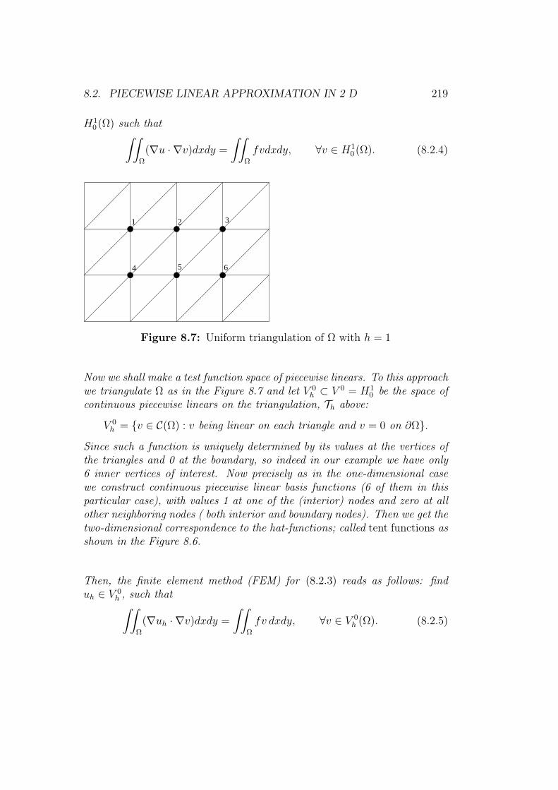
8.2. PIECEWISE LINEAR APPROXIMATION IN 2 D 219
H10 (Ω) such that
∫∫
Ω
(∇u · ∇v)dxdy =
∫∫
Ω
fvdxdy, ∀v ∈ H10 (Ω). (8.2.4)
1 2 3
4 5 6
Figure 8.7: Uniform triangulation of Ω with h = 1
Now we shall make a test function space of piecewise linears. To this approachwe triangulate Ω as in the Figure 8.7 and let V 0
h ⊂ V 0 = H10 be the space of
continuous piecewise linears on the triangulation, Th above:
V 0h = v ∈ C(Ω) : v being linear on each triangle and v = 0 on ∂Ω.
Since such a function is uniquely determined by its values at the vertices ofthe triangles and 0 at the boundary, so indeed in our example we have only6 inner vertices of interest. Now precisely as in the one-dimensional casewe construct continuous piecewise linear basis functions (6 of them in thisparticular case), with values 1 at one of the (interior) nodes and zero at allother neighboring nodes ( both interior and boundary nodes). Then we get thetwo-dimensional correspondence to the hat-functions; called tent functions asshown in the Figure 8.6.
Then, the finite element method (FEM) for (8.2.3) reads as follows: finduh ∈ V 0
h , such that∫∫
Ω
(∇uh · ∇v)dxdy =
∫∫
Ω
fv dxdy, ∀v ∈ V 0h (Ω). (8.2.5)

220CHAPTER 8. PIECEWISE POLYNOMIALS IN SEVERAL DIMENSIONS
K
The approximation procedure follows the path generalizing the 1D-case.
Below we illustrate the FEM procedure for a mixed boundary value prob-lem.
Example 8.2. Formulate the cG(1) piecewise continuous Galerkin methodfor the boundary value problem
−∆u+ u =f, x ∈ Ω;
u =0, x ∈ ∂Ω \ (Γ1 ∪ Γ2),
∇u · n =0, x ∈ Γ1 ∪ Γ2,
(8.2.6)
on the domain Ω, with outward unit normal n at the boundary (as in theFigure below). Compute the matrices for the resulting system of equationsusing the following mesh with nodes at N1, N2 and N3. We have considereda standard triangle-element T with axi-parallel sides of lenght h.
ΩΓ2
Γ1
•
• •
N1
N2N3
n
•n1•n2
•n3
T
reference element
Solution: Let V be the linear function space defined as
V := v : v ∈ H1(Ω), v = 0, on ∂Ω \ (Γ1 ∪ Γ2).

8.2. PIECEWISE LINEAR APPROXIMATION IN 2 D 221
We denote the scalar product by (·, ·), viz
(f, g) =
∫
Ω
f(x)g(x) dx.
Multiplying the differential equation by v ∈ V and integrating over Ω we get
−(∆u, v) + (u, v) = (f, v), ∀v ∈ V.
Now using Green’s formula we have that
−(∆u, v) = (∇u,∇v)−∫
∂Ω
(n · ∇u)v ds
= (∇u,∇v)−∫
∂Ω\(Γ1∪Γ2)
(n · ∇u)v ds−∫
Γ1∪Γ2
(n · ∇u)v ds
= (∇u,∇v), ∀v ∈ V,
where we used the boundary data and the definition of V . Thus the variationalformulation reads as
(∇u,∇v) + (u, v) = (f, v), ∀v ∈ V.
Let Vh be the finite element space consisting of continuous piecewise linearfunctions, on the partition as in the figure in the example, satisfying theboundary condition v = 0 on ∂Ω \ (Γ1 ∪ Γ2): Then, the cG(1) method for(8.2.6) is formulated as: Find uh ∈ Vh such that
(∇uh,∇v) + (uh, v) = (f, v) ∀v ∈ Vh
Making the “Ansatz” hh(x) =∑3
j=1 ξjϕj(x), where ϕi are the standard basisfunctions, we obtain the system of equations
3∑
j=1
ξj
(∫
Ω
∇ϕi · ∇ϕj dx+
∫
Ω
ϕiϕj dx)=
∫
Ω
fϕi dx, i = 1, 2, 3,
or in matrix form,(S +M)ξ = F,
where Sij = (∇ϕi,∇ϕj) is the stiffness matrix, Mij = (ϕi, ϕj) is the massmatrix, and Fi = (f, ϕi) is the load vector. We shall first compute the mass

222CHAPTER 8. PIECEWISE POLYNOMIALS IN SEVERAL DIMENSIONS
and stiffness matrices for the standard element T with the side length h (seeFigure above), The local basis functions and their gradients are given by
φ1(x1, x2) = 1− x1h
− x2h, ∇φ1(x1, x2) = −1
h
1
1
,
φ2(x1, x2) =x1h, ∇φ2(x1, x2) =
1
h
1
0
,
φ3(x1, x2) =x2h, ∇φ3(x1, x2) =
1
h
0
1
.
Hence, with |T | =∫Tdz = h2/2,
m11 = (φ1, φ1) =
∫
T
φ21 dx = h2
∫ 1
0
∫ 1−x2
0
(1− x1 − x2)2 dx1dx2 =
h2
12,
s11 = (∇φ1,∇φ1) =
∫
T
|∇φ1|2 dx =2
h2|T | = 1.
Alternatively, we can use the midpoint rule, which is exact for polynomialsof degree 2 (precision 3):
m11 = (φ1, φ1) =
∫
T
φ21 dx =
|T |3
3∑
j=1
φ1(xj)2 =
h2
6
(0 +
1
4+
1
4
)=h2
12,
where xj are the midpoints of the edges. Similarly we can compute the otherelements and thus obtain the local mass and stiffness matrices as
m =h2
24
2 1 1
1 2 1
1 1 2
, s =
1
2
2 −1 −1
−1 1 0
−1 0 1
.
We can now assemble the global matrices M and S from the local ones mand s, through identifying the contribution from each element sharing thesame node to the global matrices. For instance, since the node N1 is common

8.2. PIECEWISE LINEAR APPROXIMATION IN 2 D 223
to 8 triangles and represents vertices corresponding to n2 or n3 in referenceelement T so we have
M11 = 8m22 =8
12h2, S11 = 8s22 = 4,
Similarly
M12 = 2m12 =1
12h2, S12 = 2s12 = −1,
M13 = 2m23 =1
12h2, S13 = 2s23 = 0,
M22 = 4m11 =4
12h2, S22 = 4s11 = 4,
M23 = 2m12 =1
12h2, S23 = 2s12 = −1,
M33 = 3m22 =3
12h2, S33 = 3s22 = 3/2.
The remaining matrix elements are obtained by symmetry Mij = Mji, Sij =Sji. Hence,
M =h2
12
8 1 1
1 4 1
1 1 3
, S =
4 −1 0
−1 4 −1
0 −1 3/2
.
8.2.2 Error estimates for piecewise linear interpolation
In this section we make a straightforward generalization of the one dimen-sional linear interpolation estimates on an interval in the maximum norm toa two dimensional linear interpolation on a triangle. As in the 1D case, ourestimates indicate that the interpolation errors depend on the second order,this time partial derivatives of the functions being interpolated, (i.e., thecurvature of the functions), the mesh size and also the shape of the triangle.
Similar results hold in Lp norms, p = 1, 2, as well as in higher dimensionsthan 2.
To continue we assume a triangulation T = K of a two dimensionalpolygonal domain Ω. We let vi, i = 1, 2, 3 be the vertices of the triangle K.Now we consider a continuous function f defined on K and define the linearinterpolant πhf ∈ P1(K) by
πhf(vi) = f(vi), i = 1, 2, 3. (8.2.7)

224CHAPTER 8. PIECEWISE POLYNOMIALS IN SEVERAL DIMENSIONS
This is illustrated in the Figure 8.5. We shall now state some basic inter-
y
z
x
v1
v2
v3
•
•
•
K
f
πhf
Figure 8.8: The nodal interpolant of f in 2D case
polation results that we frequently use in the error estimates. The proofs ofthese results can be found, e.g. in [20].
Theorem 8.1. If f has continuous second order partial derivatives, then
‖f − πhf‖L∞(K) ≤1
2h2K ||D2f ||L∞(K), (8.2.8)
||∇(f − πhf)||L∞(K) ≤3
sin(αK)hK ||D2f ||L∞(K), (8.2.9)
where hK is the largest side of K, αK is the smallest angle of K, and
D2f =( 2∑
i,j=1
(∂2f
∂xi∂xj)2)1/2
.
Remark 8.1. Note that the gradient estimate (8.2.9) deteriorates for smallsin(αK); i.e. for the thinner triangle K. This phenomenon is avoided as-

8.2. PIECEWISE LINEAR APPROXIMATION IN 2 D 225
suming a quasi-uniform triangulation, where there is a minimum angle re-quirement for the triangles viz,
sin(αK) ≥ C, for some constant C ∈ (0, 1). (8.2.10)
8.2.3 The L2 projection
Definition 8.1. Let V be an arbitrary function space defined over Ω. TheL2 projection Pu ∈ V of a function u ∈ L2(Ω) is defined by
(u− Pu, v) = 0, ∀v ∈ V. (8.2.11)
Usually, as a special case, we take V = Vh the space of all continuous piece-wise linear functions on a triangulation Th = K of the domain Ω, and theequation (8.2.11) is then written as
(u− Phu, v) = 0, ∀v ∈ Vh. (8.2.12)
This means that, the error u − Phu is orthogonal to Vh. (8.2.12) yields alinear system of equations for the coefficients of Phu with respect to the nodalbasis of Vh.
Advantages of the L2 projection to the nodal interpolation
• The L2 projection Phu is well defined for u ∈ L2(Ω), whereas the nodalinterpolant πhu in general requires u to be continuous. Therefore the L2
projection is an alternative for the nodal interpolation for, e.g. discontinuousL2 functions.
• Letting v ≡ 1 in (8.2.11) we have that
∫
Ω
Phu dx =
∫
Ω
u dx. (8.2.13)
Thus the L2 projection conserves the total mass, whereas, in general, thenodal interpolation operator does not preserve the total mass.
• The L2 projection does not need to satisfy the (Dirichlet) boundary con-dition, whereas an interpolant has to.
• Finally we have the following error estimate for the L2 projection:

226CHAPTER 8. PIECEWISE POLYNOMIALS IN SEVERAL DIMENSIONS
Theorem 8.2. For a u with square integrable second derivative the L2 pro-jection Ph satisfies
‖u− Phu‖ ≤ Ci‖h2D2u‖. (8.2.14)
Proof. We have using (8.2.12) and the Cauchy’s inequality that
‖u− Phu‖2 = (u− Phu, u− Phu)
(u− Phu, u− v) + (u− Phu, v − Phu) = (u− Phu, u− v)
≤ ‖u− Phu‖‖u− v‖.(8.2.15)
This yields‖u− Phu‖ ≤ ‖u− v‖, ∀v ∈ Vh. (8.2.16)
Thus Phu is at least as close to u (is an at least as good approximation inthe L2-norm) as πhu. Now choosing v = πhu and recalling the interpolationtheorem above we get the desired estimate (8.2.14).
8.3 Exercises
Problem 8.1. Show that the function u : R2 → R given by u(x) = log(|x|−1), x 6=0 is a solution to the Laplace equation ∆u(x) = 0.
Problem 8.2. Show that the Laplacian of a C2 function u : R2 → R in thepolar coordinates is written by
∆u =1
r
∂
∂r
(r∂u
∂r
)+
1
r2∂2u
∂θ2. (8.3.1)
Problem 8.3. Show using (8.3.1) that the function u = a log(r)+ b, where aand b are arbitrary constants is a solution of the Laplace equation ∆u(x) = 0for x 6= 0. Are there any other solutions of the Laplace equation in R2 whichare invariant under rotation (i.e. it depends only on r = |x|)?
Problem 8.4. For a given triangle K, determine the relation between thesmallest angle τK, the triangle diameter hK and the diameter ρK of the largestinscribed circle.
Problem 8.5. Prove that a linear function in R2 is uniquely determined byits values at three points as long as they don’t lie on a straight line.
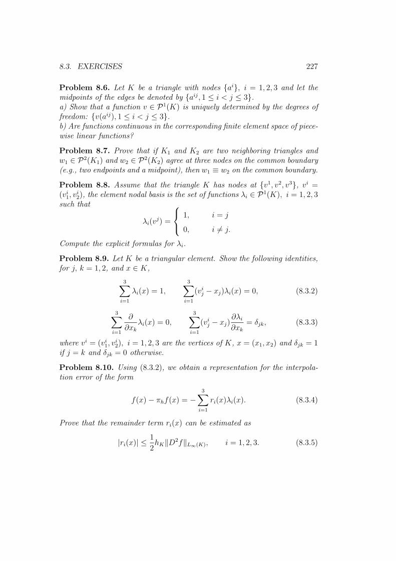
8.3. EXERCISES 227
Problem 8.6. Let K be a triangle with nodes ai, i = 1, 2, 3 and let themidpoints of the edges be denoted by aij , 1 ≤ i < j ≤ 3.a) Show that a function v ∈ P1(K) is uniquely determined by the degrees offreedom: v(aij), 1 ≤ i < j ≤ 3.b) Are functions continuous in the corresponding finite element space of piece-wise linear functions?
Problem 8.7. Prove that if K1 and K2 are two neighboring triangles andw1 ∈ P2(K1) and w2 ∈ P2(K2) agree at three nodes on the common boundary(e.g., two endpoints and a midpoint), then w1 ≡ w2 on the common boundary.
Problem 8.8. Assume that the triangle K has nodes at v1, v2, v3, vi =(vi1, v
i2), the element nodal basis is the set of functions λi ∈ P1(K), i = 1, 2, 3
such that
λi(vj) =
1, i = j
0, i 6= j.
Compute the explicit formulas for λi.
Problem 8.9. Let K be a triangular element. Show the following identities,for j, k = 1, 2, and x ∈ K,
3∑
i=1
λi(x) = 1,3∑
i=1
(vij − xj)λi(x) = 0, (8.3.2)
3∑
i=1
∂
∂xkλi(x) = 0,
3∑
i=1
(vij − xj)∂λi∂xk
= δjk, (8.3.3)
where vi = (vi1, vi2), i = 1, 2, 3 are the vertices of K, x = (x1, x2) and δjk = 1
if j = k and δjk = 0 otherwise.
Problem 8.10. Using (8.3.2), we obtain a representation for the interpola-tion error of the form
f(x)− πhf(x) = −3∑
i=1
ri(x)λi(x). (8.3.4)
Prove that the remainder term ri(x) can be estimated as
|ri(x)| ≤1
2hK‖D2f‖L∞(K), i = 1, 2, 3. (8.3.5)

228CHAPTER 8. PIECEWISE POLYNOMIALS IN SEVERAL DIMENSIONS
Hint: (I) Note that |vi − x| ≤ hK. (II) Start applying Cauchy’s inequality toshow that ∑
ij
xicijxj =∑
i
xi∑
j
cijxj.
Problem 8.11. τK is the smallest angle of a triangular element K. Showthat
maxx∈K
|∇λi(x)| ≤2
hK sin(τK).
Problem 8.12. The Euler equation for an incompressible inviscid fluid ofdensity can be written as
ut + (u · ∇)u+∇p = f, ∇ · u = 0, (8.3.6)
where u(x, t) is the velocity and p(x, t) the pressure of the fluid at the pint xat time t and f is an applied volume force (e.g., a gravitational force). Thesecond equation ∇ · u = 0 expresses the incopressibility. Prove that the firstequation follows from the Newton’s second law.
Hint: Let u = (u1, u2) with ui = ui(x(t), t), i = 1, 2 and use the chainrule to derive ui =
∂ui
∂x1u1 +
∂ui
∂x2u2 +
∂ui
∂t, i = 1, 2.
Problem 8.13. Prove that if u : R2 → R2 satisfies rotu :=(
∂u2
∂x1,−∂u1
∂x2
)= 0
in a convex domian Ω ⊂ R2, then there is a scalar function ϕ defined on Ωsuch that u = ∇ϕ in Ω.
Problem 8.14. Prove that∫Ωrotu dx =
∫Γn× u ds, where Ω is a subset of
R3 with boundary Γ with outward unit normal n.

Chapter 9
Riesz and Lax-MilgramTheorems
9.1 Preliminaries
In Chapter 5, we proved under certain assumptions that to solve a boundaryvalue problem (BVP) is equivalent to its corresponding variational formula-tion (VF) which in turn is equivalent to an associated minimization problem(MP):
BVP ⇐⇒ VF ⇐⇒ MP.
More precisely we had the following one-dimensional boundary value prob-lem:
(BV P ) :
−(a(x)u′(x)
)′= f(x), 0 < x < 1
u(0) = u(1) = 0,(9.1.1)
with the corresponding variational formulation, viz
(VF): Find u(x), with u(0) = u(1) = 0, such that
∫ 1
0
u′(x)v′(x)dx =
∫ 1
0
f(x)v(x)dx, ∀v ∈ H10 , (9.1.2)
229

230 CHAPTER 9. RIESZ AND LAX-MILGRAM THEOREMS
where H10 := H1
0 (0, 1) is the Sobolev space of all square integrable functionshaving square integrable first order derivative on (0, 1) and vanishing at theend points of the interval (0, 1):
H10 =
v :
∫ 1
0
(v(x)2 + v′(x)2
)dx <∞, v(0) = v(1) = 0
. (9.1.3)
We had also a minimization problem as:
(MP): Find u(x), with u(0) = u(1) = 0, such that u(x) minimizes the energyfunctional F given by
F (v) =1
2
∫ 1
0
v′(x)2dx−∫ 1
0
f(x)v(x)dx, ∀v ∈ H10 . (9.1.4)
Recalling Poincare inequality we may actually take instead of H10 , the space
H10 =
w : [0, 1] → R :
∫ 1
0
w′(x)2dx <∞, w(0) = w(1) = 0. (9.1.5)
Let now V be a vector space of function on (0, 1) and define a bilinear formon V by a(·, ·) : V × V → R, i.e. for α, β, x, y ∈ R and u, v, w ∈ V , we have
a(αu+ βv, w) = α · a(u, w) + β · a(v, w)a(u, xv + yw) = x · a(u, v) + y · a(u, w). (9.1.6)
Example 9.1. Let V = H10 and define
a(u, v) := (u, v) :=
∫ 1
0
u′(x)v′(x)dx, (9.1.7)
then (·, ·) is symmetric, i.e. (u, v) = (v, u), bilinear (obvious), and positivedefinite in the sense that
(u, u) ≥ 0, and (u, u) = 0 ⇐⇒ u ≡ 0.
Note that
(u, u) =
∫ 1
0
u′(x)2dx = 0 ⇐⇒ u′(x) = 0,
thus u(x) is constant and since u(0) = u(1) = 0 we have u(x) ≡ 0.

9.1. PRELIMINARIES 231
Definition 9.1. A function L : V → R is called a linear form on V , if forα, β ∈ R and u, v ∈ V ,
L(αu+ βv) = αL(u) + βL(v). (9.1.8)
Example 9.2. For f ∈ H10, let
ℓ(v) =
∫ 1
0
fv dx, ∀v ∈ H10, (9.1.9)
Then our (VF) can be restated as follows: Find u ∈ H10 such that
a(u, v) = ℓ(v), ∀v ∈ H10. (9.1.10)
Generalizing the above example, (e.g. to a Hilbert space defined below), toa bilinear form a(·, ·), and a linear form L(·), we get the following abstractproblem: Find u ∈ V , such that
a(u, v) = L(v) ∀v ∈ V. (9.1.11)
Definition 9.2. Let ‖·‖V be a norm corresponding to a scalar product (·, ·)Vdefined on V ×V . Then the bilinear form a(·, ·) is called coercive ( V-elliptic),and a(·, ·) and L(·) are continuous, if there are constants ci, i = 1, 2, 3 suchthat:
a(v, v) ≥ c1‖v‖2V , ∀v ∈ V (coercivity) (9.1.12)
|a(u, v)| ≤ c2‖u‖V ‖v‖V , ∀u, v ∈ V (a is bounded) (9.1.13)
|L(v)| ≤ c3‖v‖V , ∀v ∈ V (L is bounded). (9.1.14)
Note that since L is linear, we have, using the relation (9.1.14) above that
|L(u)− L(v)| = |L(u− v)| ≤ c3‖u− v‖V ,
which shows that L(u) −→ L(v) in R, as u −→ v, in V . Thus L iscontinuous. Similarly the relation |a(u, v)| ≤ c1‖u‖V ‖v‖V implies that thebilinear form a(·, ·) is continuous in each component.
Definition 9.3. The energy norm on V is defined by ‖v‖a =√a(v, v), v ∈
V .

232 CHAPTER 9. RIESZ AND LAX-MILGRAM THEOREMS
Recalling the relations (9.1.12) and (9.1.13) above, the energy norm satisfies
c1‖v‖2V ≤ a(v, v) = ‖v‖2a ≤ c2‖v‖2V . (9.1.15)
Hence, the energy norm ‖ • ‖a is equivalent to the abstract ‖ • ‖V norm.
Example 9.3. For the scalar product
(u, v) =
∫ 1
0
u′(x)v′(x)dx, in H10, (9.1.16)
and the norm‖u‖ =
√(u, u), (9.1.17)
the relations (9.1.12) and (9.1.13) are valid with c1 = c2 ≡ 1 :
For a general scalar product we have that
(i): (v, v) = ‖v‖2 is an identity, and
(ii): |(u, v)| ≤ ‖u‖‖v‖ is the Cauchy-Schwarz inequality sketched below:
Proof of the Cauchy’s inequality. Using the inequality 2ab ≤ a2+b2, we have
2|(u, w)| ≤ ‖u‖2 + ‖w‖2. (9.1.18)
We let w = (v/‖v‖2) (u, v), then
2|(u, w)| = 2∣∣∣(u, (u, v)
v
‖v‖2)∣∣∣ ≤ ‖u‖2 + |(u, v)|2‖v‖
2
‖v‖4 (9.1.19)
Thus
2|(u, v)|2‖v‖2 ≤ ‖u‖2 + |(u, v)|2‖v‖
2
‖v‖4 , (9.1.20)
which multiplying by ‖v‖2, gives
2|(u, v)|2 ≤ ‖u‖2 · ‖v‖2 + |(u, v)|2, (9.1.21)
and hence|(u, v)|2 ≤ ‖u‖2 · ‖v‖2, (9.1.22)
which completes the proof.

9.1. PRELIMINARIES 233
Below we further develop the abstract framework and provide general criteriato prove the existence of a unique solution for the PDEs.
Definition 9.4. A Hilbert space is a complete linear space with a scalarproduct.
To define a complete linear space we first need to define a Cauchy sequenceof real or complex numbers.
Definition 9.5. A sequence zk∞k=1 ⊂ C is a Cauchy sequence if for everyε > 0, there is an integer N > 0, such that m,n > N ⇒ |zm − zn| < ε.
Now we state, without proof, a classical theorem of analysis:
Theorem 9.1. Every Cauchy sequence in C is convergent. More precisely:If zk∞k=1 ⊂ C is a Cauchy sequence, then there is a z ∈ C, such that forevery ǫ > 0, there is an integer M > 0, such that m ≥M ⇒ |zm − z| < ε.
Definition 9.6. A linear space V (vector space) with the norm ‖ · ‖ is calledcomplete if every Cauchy sequence in V is convergent. In other words: Forevery vk∞k=1 ⊂ V with the property that for every ε1 > 0 there is an integerN > 0, such that m,n > N ⇒ ‖vm − vn‖ < ε1, (i.e. for every Cauchysequence) there is a v ∈ V such that for every ε > 0 there is an integerM > 0 such that m ≥M ⇒ ‖vm − v‖ < ε.
Theorem 9.2. The space H10 defined in (9.1.5) is a complete Hilbert space
with the norm
‖u‖ =√
(u, u) =(∫ 1
0
u′(x)2dx)1/2
. (9.1.23)
Definition 9.7. We define a functional ℓ as a mapping from a (linear) func-tion space V into R, i.e.,
ℓ : V → R. (9.1.24)
• A functional ℓ is called linear if
ℓ(u+ v) = ℓ(u) + ℓ(v) for all u, v ∈ V
ℓ(αu) = α ℓ(u) for all u ∈ V and α ∈ R.(9.1.25)

234 CHAPTER 9. RIESZ AND LAX-MILGRAM THEOREMS
• A functional is called bounded if there is a constant C such that
|ℓ(u)| ≤ C ‖u‖ for all u ∈ V (C is independnet of u)
Example 9.4. If f ∈ L2(0, 1), i.e.∫ 1
0f(x)2dx is finite, then
ℓ(v) =
∫ 1
0
f(x)v(x)dx (9.1.26)
is a bounded linear functional.
Problem 9.1. Show that ℓ, defined in example above is linear.
Problem 9.2. Prove using Cauchy’s and Poincare’s inequalities that ℓ, de-fined as in the above example , is bounded in H1
0.
9.2 Riesz and Lax-Milgram Theorems
Abstract formulations: Recalling that
(u, v) =
∫ 1
0
u′(x)v′(x)dx and ℓ(v) =
∫ 1
0
f(x)v(x)dx,
we may redefine our variational formulation (VF) and minimization problem(MP) in an abstract form as (V) and (M), respectively:
(V) Find u ∈ H10, such that (u, v) = ℓ(v) for all v ∈ H1
0.
(M) Find u ∈ H10, such that F (u) = min
v∈H10
F (v) with F (v) =1
2‖v‖2 − ℓ(v).
Theorem 9.3. There exists a unique solution for the, equivalent, problems(V) and (M).
Proof. That (V) and (M) are equivalent is shown as in Chapter 5. To proceed,we note that there exists a real number σ such that F (v) > σ for all v ∈ H1
0,(otherwise it is not possible to minimize F ): namely we can write
F (v) =1
2‖v‖2 − ℓ(v) ≥ 1
2‖v‖2 − γ‖v‖, (9.2.1)

9.2. RIESZ AND LAX-MILGRAM THEOREMS 235
where γ is the constant bounding ℓ, i.e. |ℓ(v)| ≤ γ‖v‖. But since
0 ≤ 1
2(‖v‖ − γ)2 =
1
2‖v‖2 − γ‖v‖+ 1
2γ2, (9.2.2)
thus evidently we have
F (v) ≥ 1
2‖v‖2 − γ‖v‖ ≥ −1
2γ2. (9.2.3)
Let now σ∗ be the largest real number σ such that
F (v) ≥ σ for all v ∈ H10. (9.2.4)
Take a sequence of functions uk∞k=0, such that
F (uk) −→ σ∗. (9.2.5)
To show that there exists a unique solution for (V) and (M) we shall use thefollowing two fundamental results:
(i) It is always possible to find a sequence uk∞k=0, such that F (uk) → σ∗
(because R is complete). This we already used in writing (9.2.5)
(ii) The parallelogram law (elementary linear algebra).
‖a+ b‖2 + ‖a− b‖2 = 2‖a‖2 + 2‖b‖2.
Using (ii) and the linearity of ℓ we can write
‖uk − uj‖2 = 2‖uk‖2 + 2‖uj‖2 − ‖uk + uj‖2 − 4ℓ(uk)− 4ℓ(uj) + 4ℓ(uk + uj)
= 2‖uk‖2 − 4ℓ(uk) + 2‖uj‖2 − 4ℓ(uj)− ‖uk + uj‖2 + 4ℓ(uk + uj)
= 4F (uk) + 4F (uj)− 8F(uk + uj
2
),
where we have used the definition of F (v) = 12‖v‖2 − ℓ(v) with v = uk, uj,
and v = (uk + uj)/2, respectively. In particular by linearity of ℓ:
−‖uk+uj‖2+4ℓ(uk+uj) = −4∥∥∥uk + uj
2
∥∥∥2
+8ℓ(uk + uj
2
)= −8F
(uk + uj2
).

236 CHAPTER 9. RIESZ AND LAX-MILGRAM THEOREMS
uk, k = 1, 2, . . .
σ⋆•
F (H10)
F
Figure 9.1: Illustrating the existence of a unique solution for (V ) and (M).
Now since F (uk) → σ∗ and F (uj) → σ∗, then
‖uk − uj‖2 ≤ 4F (uk) + 4F (uj)− 8σ∗ → 0, as k, j → ∞.
Hence we have shown that uk∞k=0 is a Cauchy sequence. Since uk ⊂ H10
and H10 is complete thus uk∞k=1 is a convergent sequence. Therefore, there
exists a u ∈ H10 such that u = limk→∞ uk, then, by the continuity of F we
get that
limk→∞
F (uk) = F (u). (9.2.6)
Now (9.2.5) and (9.2.6) yield F (u) = σ∗ and by (9.2.4) and the definition ofσ∗ we end up with
(M) F (u) ≤ F (v), ∀v ∈ H10, ( or F (u) < F (v), v 6= u).
(9.2.7)This in our minimization problem (M). And since (M) ⇔ (V) we concludethat: there is a unique u ∈ H1
0 , such that ℓ(v) = (u, v), ∀v ∈ H10. Note

9.2. RIESZ AND LAX-MILGRAM THEOREMS 237
that the uniqueness follows from the last step of our minimization proof:F (u+ w) ≥ F (u), ∀w ∈ H1
0.
Summing up we have proved that:
Proposition 9.1. Every bounded linear functional can be represented as ascalar product with a given function u. This u is the unique solution for both(V) and (M).
Theorem 9.4 (Riesz representation theorem). If V is a Hilbert space withthe scalar product (u, v) and norm ‖u‖ =
√(u, u), and ℓ(v) is a bounded
linear functional on V , then there is a unique u ∈ V such that
ℓ(v) = (u, v), ∀v ∈ V.
Theorem 9.5 (Lax-Milgram theorem). (A generalized version of Riesz rep-resentation theorem) Assume that ℓ(v) is a bounded linear functional on Vand a(u, v) is bilinear bounded and elliptic in V , then there is a unique u ∈ V ,such that
a(u, v) = ℓ(v), ∀v ∈ V. (9.2.8)
Remark 9.1. Here bilinear means that a(u, v) satisfies the same propertiesas a scalar product, except for symmetry
Remark 9.2. Note that if the source term f ∈ L2(Ω) then (9.1.14) holds forV = H1(Ω) and hence, in our definition of boundedness c3 = ‖f‖L2(Ω). Thequestion is whether one can reach (9.1.14) by a somewhat weaker assumptionon f than f ∈ L2(Ω)? It appears that a weaker assumption on the right handside f can be obtained using negative norm. More specifically, we define theH−1(Ω) norm of f , viz
‖f‖H−1(Ω = supv∈H1
0(Ω)
(f, v)
‖v‖V, V = H1
0 (Ω). (9.2.9)
Thus using negative norm e the equivalent norms ‖v‖H10(Ω) ≈ ‖∇v‖L2(Ω),
‖f‖H−1(Ω) ≤‖f‖L2(Ω)‖v‖L2(Ω)
‖∇v‖L2(Ω)
≤ C‖f‖L2(Ω). (9.2.10)
Hence, (9.1.14) holds with c3 = ‖f‖H−1(Ω). Therefore, it suffices that theright hand side f(x) in the Poisson’s equation satisfies a weaker assumption,i.e. f ∈ H−1(Ω) rather than f ∈ L2(Ω).

238 CHAPTER 9. RIESZ AND LAX-MILGRAM THEOREMS
Below we give some examples of verifying Lax-Milgram theorem and alsoapplications of Lax-Milgram theorem proving existence of a unique solutionfor certain differential equations of particular interest.
Example 9.5. Verify the assumptions of the Lax-Milgram Theorem and de-termine the constants of the assumptions for I = (0, 1), f ∈ L2(I), V =H1(I), ||w||2V = ||w||2L2(I)
+ ||w′||2L2(I), and
a(v, w) =
∫
I
(uw + v′w′) dx+ v(0)w(0), L(v) =
∫
I
fv dx.
Solution. It is trivial to show that a(·, ·) is bilinear and b(·) is linear. Wehave that
a(v, v) =
∫
I
v2 + (v′)2 dx+ v(0)2 ≥ ||v||2V , (9.2.11)
so that we can take c1 = 1 in (9.1.12). Further, using Cauchy-Schwarzinequality
|a(v, w)| ≤∣∣∣∫
I
vw dx∣∣∣+
∣∣∣∫
I
v′w′ dx∣∣∣+ |v(0)w(0)|
≤ ||v||L2(I)||w||L2(I) + ||v′||L2(I)||w′||L2(I) + |v(0)||w(0)|≤
(||v||L2(I) + ||v′||L2(I)
)(||w||L2(I) + ||w′||L2(I)
)+ |v(0)||w(0)|
≤√2(||v||2L2(I)
+ ||v′||2L2(I)
)1/2
·√2(||w||2L2(I)
+ ||w′||2L2(I)
)1/2
+ |v(0)||w(0)|=
√2||v||V
√2||w||V + |v(0)||w(0)|.
Now we have that
v(0) = −∫ x
0
v′(y) dy + v(x), ∀x ∈ I, (9.2.12)
and by the Mean-value theorem for the integrals there exists ξ ∈ I so thatv(ξ) =
∫ 1
0v(y) dy. Choose x = ξ in (9.2.12), then by Cauchy-Schwarz in-
equality
|v(0)| =∣∣∣−
∫ ξ
0
v′(y) dy +
∫ 1
0
v(y) dy∣∣∣
≤∫ 1
0
|v′| dy +∫ 1
0
|v| dy ≤ ||v′||L2(I) + ||v||L2(I) ≤√2||v||V ,

9.2. RIESZ AND LAX-MILGRAM THEOREMS 239
implies that|v(0)||w(0)| ≤ 2||v||V ||w||V ,
and consequently
|a(u, w)| ≤ 2||v||V ||w||V + 2||v||V ||w||V = 4||v||V ||w||V ,
so that we can take c2 = 4 in (9.1.13). Finally
|L(v)| =∣∣∣∫
I
fv dx∣∣∣ ≤ ||f ||L2(I)||v||L2(I) ≤ ||f ||L2(I)||v||V ,
taking c3 = ||f ||L2(I) in (9.1.14), all the conditions in the Lax-Milgram theo-rem are fulfilled.
Example 9.6. Let u ∈ H10 (Ω) and consider the convection-diffusion problem
−div(ε∇u+ βu) = f, in Ω ⊂ R2, u = 0 on Γ = ∂Ω, (9.2.13)
where Ω is a bounded convex polygonal domain, ε > 0 is constant, β =(β1(x), β2(x)) and f = f(x). Determine conditions in the Lax-Milgram the-orem that would guarantee existence of a unique solution for this problem.Prove a stability estimate for u i terms of ||f ||L2(Ω), ε and diam(Ω), andunder the conditions that you derived.
Solution: Recall that H10 (Ω) := w : w ∈ L2(Ω), |∇w| ∈ L2(Ω), w =
0 on ∂Ω.
a) Multiply the equation (9.2.13) by v ∈ H10 (Ω) and integrate over Ω to obtain
−∫
Ω
div(ε∇u+ βu)v dx =
∫
Ω
(ε∇u+ βu) · ∇v dx =
∫
Ω
fv dx.
Thus the variational formulation for (9.2.13) is as follows: Find u ∈ H10 (Ω)
such thata(u, v) = L(v), ∀v ∈ H1
0 (Ω), (9.2.14)
where
a(u, v) =
∫
Ω
(ε∇u+ βu) · ∇v dx,
and
L(v) =
∫
Ω
fv dx.

240 CHAPTER 9. RIESZ AND LAX-MILGRAM THEOREMS
According to the Lax-Milgram theorem, for a unique solution for (9.2.14)we need to verify that there are positive constants c1, c2, c3 such that thefollowing relations hold true
i)|a(v, w)| ≤ c1||u||H1(Ω)||w||H1(Ω), ∀v, w ∈ H1
0 (Ω),
ii)a(v, v) ≥ c2||v||2H1(Ω), ∀v ∈ H1
0 (Ω),
iii)|L(v)| ≤ c3||v||H1(Ω), ∀v ∈ H1
0 (Ω).
Now using Cauchy-Schwarz inequality we have
|L(v)| = |∫
Ω
fv dx| ≤ ||f ||L2(Ω)||v||L2(Ω) ≤ ||f ||L2(Ω)||v||H1(Ω),
hence iii) follows with c3 = ||f ||L2(Ω), and consequently the first condition isthat f ∈ L2(Ω).
Further we have that
|a(v, w)| ≤∫
Ω
|ε∇v + βv||∇w| dx ≤∫
Ω
(ε|∇v|+ |β||v|)|∇w| dx
≤(∫
Ω
(ε|∇v|+ |β||v|)2 dx)1/2(∫
Ω
|∇w|2 dx)1/2
≤√2max(ε, ||β||∞)
(∫
Ω
(|∇v|2 + v2) dx)1/2
||w||H1(Ω)
= γ||v||H1(Ω)||w||H1(Ω),
which, with c1 =√2max(ε, ||β||∞), gives i). Hence the second condition is
that β ∈ L∞(Ω).
Finally, if div β ≤ 0, then using Green’s formula
a(v, v) =
∫
Ω
(ε|∇v|2 + (β · ∇v)v
)dx =
∫
Ω
(ε|∇v|2 + (β1
∂v
∂x1+ β2
∂v
∂x2)v)dx
=
∫
Ω
(ε|∇v|2 + 1
2(β1
∂
∂x1(v)2 + β2
∂
∂x2(v)2)
)dx
=
∫
Ω
(ε|∇v|2 − 1
2(divβ)v2
)dx ≥
∫
Ω
ε|∇v|2 dx.

9.3. EXERCISES 241
Now by the Poincare’s inequality
∫
Ω
|∇v|2 dx ≥ C
∫
Ω
(|∇v|2 + v2) dx = C||v||2H1(Ω),
for some constant C = C(diam(Ω)), we have
a(v, v) ≥ c2||v||2H1(Ω), with α = Cε,
which means that ii) is valid under the condition that div β ≤ 0.
From ii), (9.2.14) (with v = u) and iii) we conclude that
c2||u||2H1(Ω) ≤ a(u, u) = L(u) ≤ c3||u||H1(Ω),
and hence a stability estimate is given by
||u||H1(Ω) ≤c3c2,
with c3 = ||f ||L2(Ω) and c2 = Cε defined above.
9.3 Exercises
Problem 9.3. Verify that the assumptions of the Lax-Milgram theorem aresatisfied for the following problems with appropriate assumptions on α andf .
(I)
−u′′ + αu = f, in (0, 1),
u(0) = u′(1) = 0, α = 0 and 1.
(II)
−u′′ + αu = f, in (0, 1),
u(0) = u(1) u′(0) = u′(1) = 0.
(III)
−u′′ = f, in (0, 1),
u(0)− u′(0) = u(1) + u′(1) = 0.

242 CHAPTER 9. RIESZ AND LAX-MILGRAM THEOREMS
Problem 9.4. Let Ω be a bounded domain in Rd with boundary Γ, show thatthere is a constant C such that for all v ∈ H1(Ω),
‖v‖L2(Γ) ≤ C‖v‖H1(Ω), (9.3.1)
where ‖v‖2H1(Ω) = ‖v‖2 + ‖∇v‖2. Hint: Use the following Green’s formula∫
Ω
v2∆ϕ =
∫
Γ
v2∂nϕ−∫
Ω
2v∇v · ∇ϕ, (9.3.2)
with ∂nϕ = 1. (9.3.1) is known as trace inequality, or trace theorem.
Problem 9.5. Let u be the solution of the following Neumann problem:
−∆u = f, in Ω ⊂ Rd,
−∂nu = ku, on Γ = ∂Ω, .
where ∂nu = n · ∇u with n being outward unit normal to Γ and k ≥ 0.
a) Show the stability estimate
‖u‖Ω ≤ CΩ(‖u‖Γ + ‖∇u‖Ω).b) Use the estimate in a) to show that ‖u‖Γ → 0 as k → ∞.
Problem 9.6. Using the trace inequality, show that the solution for the prob-lem
−∆u+ u = 0, in Ω
∂nu = g, on Γ,
satisfies the inequality
‖u‖2 + ‖∇u‖2 ≤ C‖g‖2L2(Γ).
Problem 9.7. Consider the boundary value problem
∆u = 0, in Ω ⊂ R2,
∂nu+ u = g, on Γ = ∂Ω, n is outward unit normal to Γ.
a) Show the stability estimate
||∇u||2L2(Ω) +1
2||u||2L2(Γ)
≤ 1
2||g||2L2(Γ)
.
b) Discuss, concisely, the conditions for applying the Lax-Milgram theoremto this problem.

Chapter 10
The Poisson Equation
In this chapter we shall extend the studies for the one-dimensional problemof the stationary heat conduction in Chapter 5 to solve the Poisson equationin higher dimensions, viz
−∆u = f in Ω ⊂ Rd, d = 2, 3
u = 0 on ∂Ω,(10.0.1)
where Ω is a bounded domain in Rd, with d = 2 or d = 3, with polygonalboundary Γ = ∂Ω. For a motivation of studying the Poisson equation andits applications, see Chapter 1. Below we approximate (10.0.1) using finiteelement method, prove stability results and derive a priori and a posteriorierror estimates.
10.1 Stability
To derive stability estimates for (10.0.1) we shall assume an underlying gen-eral vector space V (to be specified below) of functions as the solution space.We multiply the equation by u ∈ V and integrate over Ω to obtain
−∫
Ω
(∆u)udx =
∫
Ω
f u dx. (10.1.1)
243

244 CHAPTER 10. THE POISSON EQUATION
Using Green’s formula and the boundary condition, u = 0 on Γ, we get that
‖∇u‖2 =∫
Ω
fu ≤ ‖f‖ ‖u‖, (10.1.2)
where ‖ · ‖ denotes the usual L2(Ω)-norm.
To derive a, so called, weak stability estimate for (10.0.1) we shall need thefollowing result.
Lemma 10.1 (Poincare inequality; the 2D-version). If u satisfies (10.0.1)in a bounded domain Ω ⊂ R2. Then, there exists a constant CΩ, independentof u such that
‖u‖ ≤ CΩ‖∇u‖. (10.1.3)
Proof. Let ϕ be a function such that ∆ϕ = 1 in Ω, and 2|∇ϕ| ≤ CΩ in Ω, (itis easy to construct such a function ϕ, e.g. take ϕ(x, y) = 1
4(x2 + y2)), then
by Green’s formula and using the boundary condition we get
‖u‖2 =∫
Ω
u2∆ϕ = −∫
Ω
2u(∇u · ∇ϕ) ≤ CΩ‖u‖ ‖∇u‖. (10.1.4)
Thus, we have the desired result.
Remark 10.1. We note that in (10.1.3), as in the one-dimensional case, wehave CΩ ≈ diam(Ω), and therefore (10.1.3) is valid as long as Ω is a boundeddomain.
Combining the Poincare inequality with the inequality (10.1.2) we get thatthe following weak stability estimate holds
‖∇u‖ ≤ CΩ‖f‖. (10.1.5)
Problem 10.1. Derive corresponding stability estimates for the followingNeumann boundary value problem:
−∆u+ u = f, in Ω
∂u∂n
= 0, on Γ = ∂Ω.(10.1.6)

10.2. ERROR ESTIMATES FOR THE CG(1) FEM 245
10.2 Error Estimates for the CG(1) FEM
We start formulating the weak form for the problem (10.0.1). We multiplythe equation by a test function, integrate over Ω and use Green’s formula.Then, the variational formulation reads as follows: Find u ∈ H1
0 (Ω) suchthat
(V F ) :
∫
Ω
∇u · ∇v dx =
∫
Ω
fv dx, ∀v ∈ H10 (Ω). (10.2.1)
We prepare for a finite element method where we shall approximate theexact solution u(x) by a suitable discrete solution U(x) in a certain finitedimensional subspace of H1
0 (Ω). To this approach let Th = K : ∪K = Ωbe a triangulation of the domain Ω by element K with the maximal diameterh = maxK diam(K). To be specific we shall consider the cG(1) methoddescribing continuous piecewise linear approximations for the solution u ∈H1
0 (Ω) in a finite dimensional subspace. Thus we have the test and trialfunction space given as
V 0h = v(x) : v is continuous, piecewise linear on Th, and v = 0 onΓ = ∂Ω.
Observe that V 0h ⊂ H1
0 (Ω) is associated to the partition Th. We assume ninterior partition nodes with ϕj, j = 1, 2, . . . , n being the corresponding basisfunctions, such that ϕj(x) is continuous, linear on each K, and
ϕj(Ni) =
1 for i = j
0 for i 6= j.(10.2.2)
Here N1, N2, . . . , Nn are the inner nodes in the triangulation, and dim V 0h =
n.
Now we set the approximate solution uh(x) to be a linear combination of thebasis functions ϕj, j = 1, . . . , n:
uh(x) = uh,1ϕ1(x) + uh,2ϕ2(x) + . . .+ uh,nϕn(x), (10.2.3)
and seek the coefficients uh,j = uh(Nj), i.e., the nodal values of uh(x), at thenodes Nj, 1 ≤ j ≤ n, so that

246 CHAPTER 10. THE POISSON EQUATION
∫
Ω
∇uh · ∇v dx =
∫
Ω
f v dx, ∀v ∈ V 0h , (10.2.4)
or equivalently
(FEM)
∫
Ω
∇uh · ∇ϕi dx =
∫
Ω
f ϕi dx, for i = 1, 2, . . . n. (10.2.5)
Note that every v ∈ V 0h can be represented by a linear combination of ϕjnj=1:
v(x) = v(N1)ϕ1(x) + v(N2)ϕ2(x) + . . .+ v(Nn)ϕn(x). (10.2.6)
Theorem 10.1 (The a priori error estimate for the gradient ∇u − ∇uh).Let e = u− uh represent the error in the above continuous, piecewise linear,finite element approximation of the solution for (10.0.1). Then we have
‖∇e‖ = ‖∇(u− uh)‖ ≤ C‖hD2u‖. (10.2.7)
Proof. For the error e = u − uh we have ∇e = ∇(u − uh) = ∇u − ∇uh.Subtracting (10.2.5) from the (10.2.1) where we restrict v to V 0
h , we obtainthe Galerkin Orthogonality:
∫
Ω
(∇u−∇uh) · ∇v dx =
∫
Ω
∇e · ∇v dx = 0, ∀v ∈ V 0h . (10.2.8)
Further we may write
‖∇e‖2 =∫
Ω
∇e·∇e dx =
∫
Ω
∇e·∇(u−uh) dx =
∫
Ω
∇e·∇u dx−∫
Ω
∇e·∇uh dx.
Now using the Galerkin orthogonality (10.2.8), since uh ∈ V 0h we have the last
integral above:∫Ω∇e ·∇uh dx = 0. Hence removing the vanishing ∇uh-term
and inserting∫Ω∇e · ∇v dx = 0 for any arbitrary v ∈ V 0
h we have that
‖∇e‖2 =∫
Ω
∇e·∇udx−∫
Ω
∇e·∇vdx =
∫
Ω
∇e·∇(u−v)dx ≤ ‖∇e‖ ‖∇(u−v)‖.
Thus‖∇(u− uh)‖ ≤ ‖∇(u− v)‖, ∀v ∈ V 0
h . (10.2.9)

10.2. ERROR ESTIMATES FOR THE CG(1) FEM 247
uh
u
V 0h
u− uh
•
Figure 10.1: The orthogonal (L2) projection of u on V 0h .
That is, in the L2-norm, the gradient of the finite element solution, ∇uhis closer to the gradient of the exact solution, ∇u, than the gradient ∇vof any other v in V 0
h . In other words, measuring in H10 -norm, the error
u− uh is orthogonal to V 0h . It is possible to show that there is a v ∈ V 0
h (aninterpolant), such that
‖∇(u− v)‖ ≤ C‖hD2u‖, (10.2.10)
where h = h(x) = diam(K) for x ∈ K and C is a constant independent of h.This is the case, for example, if v interpolates u at the nodes Ni.
Combining (10.2.9) and (10.2.10) we get
‖∇e‖ = ‖∇(u− uh)‖ ≤ C‖hD2u‖, (10.2.11)
which is indicating that the error is small if h(x) is sufficiently small depend-ing on D2u. See the Figure below.
To prove an a priori error estimate for the solution we shall use the followingresult.

248 CHAPTER 10. THE POISSON EQUATION
x2
x3
x1
N1
N2
N3
•
•
•
K
u
πhu
Figure 10.2: The nodal interpolant of u in 2D case
Lemma 10.2 (regularity lemma). Assume that Ω has no reentrent corners(Ω is convex). We have for u ∈ H2(Ω); with u = 0 or (∂u
∂n= 0) on ∂Ω, that
‖D2u‖ ≤ CΩ ‖∆u‖, (10.2.12)
where
D2u = (u2xx + 2u2xy + u2yy)1/2. (10.2.13)
We postpone the proof of this lemma and first derive the error estimate.
Theorem 10.2 (a priori error estimate for the solution e = u − uh). For ageneral mesh we have the following a priori error estimate for the solutionof the Poisson equation (10.0.1),
‖e‖ = ‖u− uh‖ ≤ C2CΩ (maxΩ
h) ‖hD2u‖, (10.2.14)
where C is a constant (generated twice).

10.2. ERROR ESTIMATES FOR THE CG(1) FEM 249
•
•
•
•
•
•
•
•
•
••
•
•••
•
h large h small
D2u large
D2u small
Figure 10.3: The adaptivity principle: to refine mesh for large D2u
Proof. Let ϕ be the solution of the dual problem
−∆ϕ = e, in Ω
ϕ = 0, on ∂Ω.(10.2.15)
Then, we have using Green’s formula that
‖e‖2 =∫
Ω
e(−∆ϕ)dx =
∫
Ω
∇e · ∇ϕ dx =
∫
Ω
∇e · ∇(ϕ− v) dx
≤ ‖∇e‖‖∇(ϕ− v)‖, ∀v ∈ V 0h ,
(10.2.16)
where in the last equality we have used the Galerkin orthogonality. We nowchoose v (e.g. as an interpolant of ϕ) such that
‖∇(ϕ− v)‖ ≤ C‖hD2ϕ‖ ≤ C(h)‖D2ϕ‖. (10.2.17)
Applying the lemma to ϕ, we get
‖D2ϕ‖ ≤ CΩ ‖∆ϕ‖ = CΩ‖e‖. (10.2.18)

250 CHAPTER 10. THE POISSON EQUATION
Finally, combining (10.2.11)-(10.2.18) yields
‖e‖2 ≤ ‖∇e‖ ‖∇(ϕ− v)‖ ≤ ‖∇e‖Ch ‖D2ϕ‖≤ ‖∇e‖C(h)CΩ‖e‖ ≤ C‖hD2u‖C (h)CΩ‖e‖.
(10.2.19)
Thus we have obtained the desired a priori error estimate
‖e‖ = ‖u− uh‖ ≤ C2CΩ (h) ‖hD2u‖. (10.2.20)
Corollary 10.1 (strong stability estimate). Using the Lemma 10.2, for apiecewise linear approximation, the a priori error estimate (10.2.20) can bewritten as the following strong stability estimate,
‖u− uh‖ ≤ C2C2Ω (h)2 ‖f‖. (10.2.21)
Theorem 10.3 ( a posteriori error estimate). Let u be the solution of thePoisson equation (10.0.1) and uh its continuous piecewise linear finite ele-ment approximation. Then, there is constant C, independent of u and h,such that
‖u− uh‖ ≤ C ‖h2r‖, (10.2.22)
where r = f + ∆huh is the residual with ∆h being the discrete Laplaciandefined by
(∆huh, v) =∑
K∈Th
(∇uh,∇v)K . (10.2.23)
Proof. We start considering the following dual problem
−∆ϕ(x) = e(x), x ∈ Ω,
ϕ(x) = 0, x ∈ ∂Ω, e(x) = u(x)− uh(x).(10.2.24)
Then e(x) = 0, ∀x ∈ ∂Ω, and using Green’s formula we have that
‖e‖2 =∫
Ω
e e dx =
∫
Ω
e(−∆ϕ)dx =
∫
Ω
∇e · ∇ϕdx. (10.2.25)

10.2. ERROR ESTIMATES FOR THE CG(1) FEM 251
Thus by the Galerkin orthogonality (10.2.8) and using the boundary data:ϕ(x) = 0, ∀x ∈ ∂Ω, we get
‖e‖2 =∫
Ω
∇e · ∇ϕdx−∫
Ω
∇e · ∇vdx =
∫
Ω
∇e · ∇(ϕ− v) dx
=
∫
Ω
(−∆e)(ϕ− v) dx ≤ ‖h2r‖ ‖h−2(ϕ− v)‖
≤ C ‖h2r‖ ‖∆ϕ‖ ≤ C ‖h2r‖ ‖e‖,
(10.2.26)
where we use the fact that the −∆e = −∆u+∆huh + [∂uh
∂n] = f +∆huh = r
is the residual and choose v as an interpolant of ϕ, so that
‖h−2(ϕ− v)‖ ≤ C‖D2ϕ‖ ≤ C CΩ‖∆ϕ‖.
Thus, the final result reads as
‖u− uh‖ ≤ CΩ ‖h2r‖. (10.2.27)
Corollary 10.2 (strong stability estimate). Observe that for piecewise linearapproximations ∆uh = 0 but ∆huh 6= 0 on each element K. If ∆huh = 0 oneach element K then r ≡ f and our a posteriori error estimate above can beviewed as a strong stability estimate
‖e‖ ≤ C ‖h2f‖. (10.2.28)
Problem 10.2. Show that ‖∇(u− uh)‖ ≤ C‖hr‖.Problem 10.3. Verify that for v being the interpolant of ϕ, we have
‖e‖ ≤ C ‖h2f‖ ×
‖h−2 (ϕ− v)‖ ≤ C ‖∆ϕ‖, and
‖h−1(ϕ− v)‖ ≤ C ‖∇ϕ‖.(10.2.29)
Problem 10.4. Derive the estimate corresponding to (10.2.27) for the one-dimensional case.
We now return to the proof of Lemma 10.2. One can show that, in the lemma,for a convex Ω, the constant CΩ ≤ 1. Otherwise CΩ > 1 and increases withthe degree of the singularity of a corner point at the boundary of the domainΩ. With Ω having a reenterant we have that CΩ = ∞.

252 CHAPTER 10. THE POISSON EQUATION
10.2.1 Proof of the regularity Lemma
Proof. Let now Ω be a rectangular domain and set u = 0 on ∂Ω. We havethen
‖∆u‖2 =∫
Ω
(uxx + uyy)2dxdy =
∫
Ω
(u2xx + 2uxxuyy + u2yy) dxdy. (10.2.30)
Applying Green’s formula (in x-direction) for the rectangular domain Ω wecan write (note that partial derivatives of higher order appears),
∫
Ω
uxxuyydxdy =
∫
∂Ω
(ux · nx)uyy ds−∫
Ω
ux uyyx︸︷︷︸=uxyy
dxdy. (10.2.31)
Once again by Green’s formula ( “with v = ux and ∆w = uxyy”),
∫
Ω
uxuxyydxdy =
∫
∂Ω
ux(uyx · ny)ds−∫
Ω
uxyuxy dxdy. (10.2.32)
Inserting (10.2.32) in (10.2.31) yields
∫
Ω
uxxuyy dxdy =
∫
∂Ω
(uxuyynx − uxuyxny)ds+
∫
Ω
uxyuxy dxdy. (10.2.33)
Now, as we can see from the figure, we have that (uxuyynx − uxuyxny) = 0,on ∂Ω and hence
∫
Ω
uxxuyydxdy =
∫
Ω
uxyuxydxdy =
∫
Ω
u2xy dxdy. (10.2.34)
Thus, in this case,
‖∆u‖2 =∫
Ω
(uxx + uyy)2dxdy =
∫
Ω
(u2xx + 2u2xy + u2yy)dxdy = ‖D2u‖2,
and the proof is complete by a constant CΩ ≡ 1. The general case of apolygonal domain, easily, follows from this proof.

10.3. EXERCISES 253
n(0, y) = (−1, 0) n(a, y) = (1, 0)
n(x, 0) = (0,−1)
n(x, b) = (0, 1)
Ω
b
a
uy = 0uy = 0
ux = 0
ux = 0
Figure 10.4: A rectangular domain Ω with its outward unit normals
10.3 Exercises
Problem 10.5. Consider the following two dimensional problem:
−∆u = 1, in Ω
u = 0, on ΓD
∂u∂n
= 0, on ΓN
(10.3.1)
See figure below
Triangulate Ω as in the figure and let
U(x) = U1ϕ1(x) + . . .+ U16ϕ16(x),
where x = (x1, x2) and ϕj, j = 1, . . . 16 are the basis functions, see Fig.below, and determine U1, . . . U16 so that
∫
Ω
∇U · ∇ϕjdx =
∫
Ω
ϕjdx, j = 1, 2, . . . , 16.

254 CHAPTER 10. THE POISSON EQUATION
1
Γ
x2 x2
ΓN
Γ
ΓD Ω
1
1
1
N
D
xx1 1
N1
N15
ϕ1
ϕ15
Problem 10.6. Generalize the procedure in the previous problem to the fol-lowing case with mesh-size=h.
−∇(a∇u) = f, in Ω
u = 0, on ΓD
a∂u∂n
= 7, on ΓN
, where
a = 1 for x1 <12
a = 2 for x1 >12
f = x2.
Problem 10.7. Consider the Dirichlet problem
−∇ · (a(x)∇u(x)) = f(x), x ∈ Ω ⊂ R2, u(x) = 0, for x ∈ ∂Ω.

10.3. EXERCISES 255
Assume that c0 and c1 are constants such that 0 < c0 ≤ a(x) ≤ c1, ∀x ∈ Ωand let U be a Galerkin approximation of u in a subspace M of H1
0 (Ω). Provethe a priori error estimate
||u− U ||H10(Ω) ≤
c1c0
infχ∈M
||u− χ||H10(Ω).
Problem 10.8. Determine the stiffness matrix and load vector if the cG(1)finite element method applied to the Poisson’s equation on a triangulationwith triangles of side length 1/2 in both x1- and x2-directions:
−∆u = 1, in Ω = (x1, x2) : 0 < x1 < 2, 0 < x2 < 1,u = 0, on Γ1 = (0, x2) ∪ (x1, 0) ∪ (x1, 1),∂u∂n
= 0, on Γ2 = (2, x2) : 0 ≤ x2 ≤ 1.
Problem 10.9. Let Ω = (0, 2)× (0, 2), B1 = ∂Ω \B2 and B2 = 2× (0, 2).Determine the stiffness matrix and load vector in the cG(1) solution for theproblem
−∂2u∂x2
1
− 2∂2u∂x2
2
= 1, in Ω = (0, 2)× (0, 2),
u = 0, on B1,∂u∂x1
= 0, on B2,
with piecewise linear approximation applied on the triangulation below:
1
2
1
B
B
B
B
2
1
x
x
2
1
2

256 CHAPTER 10. THE POISSON EQUATION
Problem 10.10. Determine the stiffness matrix and load vector if the cG(1)finite element method with piecewise linear approximation is applied to thefollowing Poisson’s equation with mixed boundary conditions:
−∆u = 1, on Ω = (0, 1)× (0, 1),
∂u∂n
= 0, for x1 = 1,
u = 0, for x ∈ ∂Ω \ x1 = 1,
on a triangulation with triangles of side length 1/4 in the x1-direction and1/2 in the x2-direction.
Problem 10.11. Formulate the cG(1) method for the boundary value prob-lem
−∆u+ u = f, x ∈ Ω; u = 0, x ∈ ∂Ω.
Write down the matrix form of the resulting system of equations using thefollowing uniform mesh:
1 2
34
h
h
x2
x1
T

Chapter 11
The Initial Boundary ValueProblems in RN
This chapter is devoted to the study of time dependent problems formulatedin spatial domain in RN , N ≥ 2. More specifically we shall consider the finiteelement methods for two fundamental equations: the heat equation and the waveequation. In this setting we have already studied time discretizations as well asa concise finite element analysis of the Laplace’s equation in Chapters 6 and 10,respectively. Here we shall derive certain stability estimates for these equationsand construct fully discrete schemes for temporal and spatial discretizations. Wealso formulate some convergence results that can be viewed as a combination oferror estimates in Chapters 6 and 10. Detailed proofs for a priori and a posteriorierror estimates are direct generalization of the results of Chapter 7 for one spacedimension and can be found in, e.g. Thomee [53] and Eriksson et al. [20].
11.1 The heat equation in RN
In this section we shall study the stability of the heat equation in RN , N ≥ 2.Here our concern will be those aspects of the stability estimates for the higherdimensional case that are not a direct consequence of the study of the one-dimensional problem addressed in Chapter 7.
257

258CHAPTER 11. THE INITIAL BOUNDARYVALUE PROBLEMS IN RN
The initial boundary value problem for the heat conduction can be formu-lated as
u(x, t)−∆u(x, t) = f(x, t), for (x, t) ∈ Ω ⊂ Rd, d = 1, 2, 3 (DE)
u(x, t) = 0, x ∈ Γ := ∂Ω, 0 < t ≤ T, (BC)
u(x, 0) = u0(x), for x ∈ Ω. (IC)
(11.1.1)The equation (11.1.1) is of parabolic type with significant smoothing andstability properties. It can also be used as a model for a variety of physicalphenomena involving diffusion processes. Some important physical proper-ties of (11.1.1) are addressed in Chapter 1. Here, we shall focus on thestability concept and also construction of the fully discrete schemes, whichis a combination of the discretization procedure in Chapters 6 and 10. Fordetails in a priori and a posteriori analysis we refer the reader to Chapter 16in [20].
11.1.1 The fundamental solution
Let us consider the stationary heat conduction in the whole two dimensionalEuclidean space:
u(x, t)−∆u(x, t) = 0, for (x, t) ∈ R2 × (0,∞)
u(x, 0) = u0(x), for x ∈ R2(11.1.2)
The solution to (11.1.2) with the Dirac delta function as its initial data:u0(x) = δ0(x) is called the Fundamental solution of the heat equation (11.1.2)which we denote by E(x, t). One may easily verify that
E(x, t) =1
4πtexp
(− |x|2
4t
). (11.1.3)
For a general u0 the solution for (11.1.2) is expressed in terms of fundamentalsolution and is obtained through convolution of u0 and E, viz
u(x, t) =1
4πt
∫
R2
u0(y) exp(− |x− y|2
4t
)dy. (11.1.4)

11.1. THE HEAT EQUATION IN RN 259
11.1.2 Stability
The stability estimates for the heat equation (11.1.1) are summarized intheorem below. It roughly states a control of certain energy norms of thesolution u by the L2 norm of the initial data u0. Meanwhile, in severalestimates, various singularities at t = 0 are clearly pronounced.
Theorem 11.1 (Energy estimates). Let f ≡ 0. Then, the solution u of theproblem (11.1.1) satisfies the following stability estimates
max(‖u(·, t)‖2, 2
∫ t
0
‖∇u‖2(s) ds)≤ ‖u0‖2 (11.1.5)
‖∇u(·, t)‖ ≤ 1√2 t
‖u0‖ (11.1.6)
(∫ t
0
s‖∆u(·, s)‖2 ds)1/2
≤ 1
2‖u0‖ (11.1.7)
‖∆u(·, t)‖ ≤ 1√2 t
‖u0‖ (11.1.8)
For ε > 0 small,
∫ t
ε
‖u(·, s)‖ ds ≤ 1
2
√lnt
ε‖u0‖. (11.1.9)
Note that (11.1.9) indicates strong instabilities for ε (as well as t) close to 0.This yields the splitting strategy used in error analysis below.
Proof. To derive the first two estimates in (11.1.5) we multiply (11.1.1) by uand integrate over Ω, to get
∫
Ω
uu dx−∫
Ω
(∆u)u dx = 0. (11.1.10)
Note that uu = 12
ddtu2. Further, using Green’s formula with the Dirichlet
boundary data, u = 0 on Γ, we have that
−∫
Ω
(∆u)u dx = −∫
Γ
(∇u ·n) u ds+∫
Ω
∇u ·∇u dx =
∫
Ω
|∇u|2 dx. (11.1.11)
Thus equation (11.1.10) can be written in the following two equivalent forms:
1
2
d
dt
∫
Ω
u2dx+
∫
Ω
|∇u|2dx = 0 ⇐⇒ 1
2
d
dt‖u‖2 + ‖∇u‖2 = 0, (11.1.12)

260CHAPTER 11. THE INITIAL BOUNDARYVALUE PROBLEMS IN RN
where ‖ · ‖ denotes the L2(Ω) norm. We substitute t by s and integrate theequation (11.1.12) over s ∈ (0, t) to get
1
2
∫ t
0
d
ds‖u‖2(s)ds+
∫ t
0
‖∇u‖2(s)ds = 1
2‖u‖2(t)−1
2‖u‖2(0)+
∫ t
0
‖∇u‖2ds = 0.
Hence, inserting the initial data u(0) = u0 we have
‖u‖2(t) + 2
∫ t
0
‖∇u‖2(s) ds = ‖u0‖2. (11.1.13)
In particular, we have our first two stability estimates
‖u‖(t) ≤ ‖u0‖, and
∫ t
0
‖∇u‖2(s) ds ≤ 1
2‖u0‖. (11.1.14)
To derive (11.1.6) and (11.1.7), since u = ∆u, and we need to estimate theL2-norm of u, so we multiply the equation, u − ∆u = 0, by −t∆u andintegrate over Ω to obtain
−t∫
Ω
u∆u dx+ t
∫
Ω
(∆u)2 dx = 0. (11.1.15)
Using Green’s formula (u = 0 on Γ =⇒ u = 0 on Γ) yields∫
Ω
u∆u dx = −∫
Ω
∇u · ∇u dx = −1
2
d
dt‖∇u‖2, (11.1.16)
so that (11.1.15) can be rewritten as
t1
2
d
dt‖∇u‖2 + t ‖∆u‖2 = 0. (11.1.17)
Now using the relation t ddt‖∇u‖2 = d
dt(t‖∇u‖2) − ‖∇u‖2, (11.1.17) can be
rewritten as
d
dt
(t‖∇u‖2
)+ 2t‖∆u‖2 = ‖∇u‖2. (11.1.18)
Once again we substitute t by s and integrate over (0, t) to get
∫ t
0
d
ds
(s‖∇u‖2(s)
)ds+ 2
∫ t
0
s‖∆u‖2(s)ds =∫ t
0
‖∇u‖2(s)ds.

11.1. THE HEAT EQUATION IN RN 261
Using (11.1.14), the last equality is estimated as
t ‖∇u‖2(t) + 2
∫ t
0
s ‖∆u‖2(s) ds ≤ 1
2‖u0‖2. (11.1.19)
In particular, we have
‖∇u‖(t) ≤ 1√2t‖u0‖ and
(∫ t
0
s‖∆u‖2(s) ds)1/2
≤ 1
2‖u0‖,
which are our third and fourth stability estimates (11.1.6) and (11.1.7). Thestability estimate (11.1.8) is proved analogously. Now using (11.1.1): (u =∆u) and (11.1.8) we may write
∫ t
ε
‖u‖(s)ds ≤ 1√2‖u0‖
∫ t
ε
1
sds =
1√2lnt
ε‖u0‖ (11.1.20)
or more carefully
∫ t
ε
‖u‖(s)ds =∫ t
ε
‖∆u‖(s)ds =∫ t
ε
1 ‖∆u‖(s)ds =∫ t
ε
1√s
√s‖∆u‖(s)ds
≤(∫ t
ε
s−1 ds)1/2 (∫ t
ε
s‖∆u‖2(s) ds)1/2
≤ 1
2
√lnt
ε‖u0‖,
where in the last two inequalities we use Cauchy Schwarz inequality and(11.1.7), respectively. This yields (11.1.9) and the proof is complete.
Problem 11.1. Show that ‖∇u(t)‖ ≤ ‖∇u0‖ (the stability estimate for thegradient). Hint: Assume f = 0, multiply (11.1.1) by −∆u and integrate overΩ.
Is this inequality valid for u0 = constant?
Problem 11.2. Derive the corresponding estimate for Neumann boundarycondition:
∂u
∂n= 0. (11.1.21)

262CHAPTER 11. THE INITIAL BOUNDARYVALUE PROBLEMS IN RN
11.1.3 A finite element method for the heat equation
For the time discretization of (11.1.1) we shall consider a partition of thetime interval I = [0, T ] : 0 = t0 < t1 < . . . < tN = T into sub-intervalsIn = (tn−1, tn) of length kn = tn − tn−1. Then, we divide the space-time slabSn = Ω × In into prisms K × In, where K ∈ Tn and Tn is a triangulationof Ω with the mesh function hn. We construct a finite element mesh basedon approximations by continuous piecewise linear functions in space anddiscontinuous polynomials of degree r in time. We shall refer to this methodas cG(1)dG(r) method. We define the trial space viz,
W(r)k = v(x, t) : v|Sn
∈ W(r)kn , n = 1, 2, . . . , N,
where
W(r)kn = v(x, t) : v(x, t) =
r∑
j=0
tjψj(x), ψj ∈ Vn, (x, t) ∈ Sn,
with Vn = Vhnis the space of continuous piecewise linear functions vanishing
on Γ associated to Tn. Generally, the functions in W(r)k are discontinuous
across the discrete time levels tn with jump discontinuities [wn] = w+n − w−
n
and w±m = lims→0± w(tn + s).
The cG(1)dG(r) method is based on a variational formulation for (11.1.1),
viz: Find U ∈ W(r)k such that for n = 1, 2, . . . , N ,
∫
In
((U , v) + (∇U,∇v)
)dt+
([Un−1], v
+n−1
)=
∫
In
(f, v) dt, ∀v ∈ W(r)kn ,
(11.1.22)where U−
0 = u0 and(·, ·) is the L2(Ω) inner product.
Using the discrete Laplacian ∆hn, in the case of r = 0, we may write (11.1.22)
as follows: find Un ∈ Vn such that
(I − kn∆n)Un = PnUn−1 +
∫
In
Pnf dt, (11.1.23)
where Un = U−n = U |In ∈ Vn , and Pn is the L2(Ω) projection onto Vn. Note
that the initial data Un−1 ∈ Vn−1 from the previous time interval In−1 is

11.1. THE HEAT EQUATION IN RN 263
projected into the space Vn. If Vn−1 ⊂ Vn, then PnUn−1 = Un−1. For thecase r = 1, writing U(t) = Φn + (t − tn−1)Ψn on In with Φn, Ψn ∈ Vn, thevariational formulation (11.1.22) takes the following form
(I − kn∆n)Φn + (I − kn2∆n)Ψn = PnUn−1 +
∫InPnf dt,
(12I − kn
3∆n)Ψn − kn
2∆nΦn =
∫In
t−tn−1
knPnf dt,
(11.1.24)
and gives a system of equations for Φn and Ψn.
11.1.4 Constructing the discrete equations
To construct the matrix equation that determines Un in the case r = 0according (11.1.23), we let ϕn,j denote the nodal basis for Vn associated withJn interior nodes of Tn, then we can write Un as
Un =Jn∑
j=1
ξn,jϕn,j.
Here ξn,j are the nodal values of Un. Let us denote the vector coefficients byξn = (ξn,j). We denote the Jn × Jn mass matrix by Mn, stiffness matrix bySn and the Jn × 1 data vector by bn, with the associated elements
(Mn)i,j = (ϕn,j, ϕn,i), (Sn)i,j = (∇ϕn,j,∇ϕn,i), and (bn)i =
∫ tn
tn−1
(f, ϕn,i),
for 1 ≤ i, j ≤ Jn. Finally, we denote the Jn × Jn−1 = matrix Mn−1,n withentries
(Mn−1,n)ij = (ϕn,j, ϕn−1,i), 1 ≤ i ≤ Jn, 1 ≤ j ≤ Jn−1. (11.1.25)
Now, the discrete equation for cG(1)dG(0) approximation on In reads asfollows: fins ξn such that
(Mn + knSn)ξn =Mn−1,nξn−1 + bn. (11.1.26)
One can easily verify that the coefficient matrix of the system (11.1.26) issparse, symmetric, and positive definite, which can be solved by a direct oran iterative algorithm.

264CHAPTER 11. THE INITIAL BOUNDARYVALUE PROBLEMS IN RN
11.1.5 An apriori error estimate
To derive a priori (or a posteriori) error estimates for the heat equation inhigher dimensions is a rather involved procedure. Below we outline the pre-requisites and formulate an a priori error estimate theorem without a proof.Detailed studies of the error analysis, for both heat and wave equations, canbe found in [20]
We assume that there are positive constants αi, i = 1, 2, with α2 sufficientlysmall, such that for n = 1, . . . , N ,
α1kn ≤ kn+1 ≤ α−11 kn, (11.1.27)
α1hn(x) ≤ hn+1(x) ≤ α−11 hn, x ∈ Ω (11.1.28)
(maxx∈Ω
h(x))2 ≤ α2kn, (11.1.29)
The relation (11.1.29) enters if Vn−1 * Vn. An a priori error estimate is thengiven as:
Theorem 11.2. If Ω is convex and α2 sufficiently small, then there is a con-stant Ci depending only on τ (which is the minimum angle in the triangula-tion of Ω) and αi, i = 1, 2, such that for N ≥ 1, and under the assumptions(11.1.27)-(11.1.29),
‖u(tN)− UN‖ ≤ CiLN max1≤n≤N
(kn‖u‖In + ‖h2nD2u‖In), (11.1.30)
where
LN = 2 + max1≤n≤N
max(
log(tnkn
))1/2
, log(tnkn
).
11.2 Exercises
Problem 11.3. Consider the following general form of the heat equation
ut(x, t)−∆u(x, t) = f(x, t), for x ∈ Ω, 0 < t ≤ T,
u(x, t) = 0, for x ∈ Γ, 0 < t ≤ T,
u(x, 0) = u0(x), for x ∈ Ω,
(11.2.1)

11.2. EXERCISES 265
where Ω ∈ R2 with boundary Γ. Let u be the solution of (11.2.1) with amodified initial data u0(x) = u0(x)ε(x).
a) Show that w := u− u solves (11.2.1) with initial data w0(x) = ε(x).
b) Give estimates for the difference between u and u.
c) Prove that the solution of (11.2.1) is unique.
Problem 11.4. Formulate the equation for cG(1)dG(1) for the two-dimensionalheat equation using the discrete Laplacian.
Problem 11.5. In two dimensions the heat equation, in the case of radialsymmetry, can be formulated as ru−(ru′r)
′r = rf , where r = |x| and w′
r =∂w∂r.
a) Verify that u = 14πt
exp(− r2
4t) is a solution for the homogeneous equation
(f = 0) with the initial data being the Dirac δ function u(r, 0) = δ(r).
b) Sketching u(r, t) for t = 1 and t = 0.01, deduce that u(r, t) → 0 ast→ 0 for r > 0.
c) Show that∫R2 u(x, t) dx = 2π
∫∞0u(r, t) r dr = 1 for all t.
d) Determine a stationary solution to the heat equation with data
f =
1/(πε)2, for r < ε,
0, otherwise.
e) Determine the fundamental solution corresponding to f = δ, lettingε→ 0.
Problem 11.6. Consider the Schrodinger equation
iut −∆u = 0, in Ω, u = 0, on ∂Ω.
where i =√−1 and u = u1 + iu2.
a) Show that the total probability∫Ω|u|2 is independent of the time.
Hint: Multiplying by u = u1 − iu2, and consider the imaginary part

266CHAPTER 11. THE INITIAL BOUNDARYVALUE PROBLEMS IN RN
b) Consider the corresponding eigenvalue problem, i.e, find the eigenvalueλ and the corresponding eigenfunction u 6= 0 such that
−∆u = λu in Ω, u = 0, on ∂Ω.
Show that λ > 0 and give the relationship between the norms ‖u‖ and‖∇u‖ for the corresponding eigenfunction u.
c) Determine (in terms of the smallest eigenvalue λ1), the smallest possi-ble value for the constant C in the Poincare estimate
‖u‖ ≤ C‖∇u‖,
derived for all solutions u vanishing at the boundary (u = 0, on ∂Ω).
Problem 11.7. Consider the initial-boundary value problem
ut(x, t)−∆u(x, t) = f(x, t), for x ∈ Ω, t > 0,
u(x, t) = 0, for x ∈ Γ, t > 0,
u(x, 0) = u0(x), for x ∈ Ω,
(11.2.2)
a) Prove (with ‖u‖ = (∫Ωu2 dx)1/2) that
‖u(t)‖2 +∫ t
0
‖∇u(s)‖2 ds ≤ ‖u0‖2 +∫ t
0
‖f(s)‖2 ds
‖∇u(t)‖2 +∫ t
0
‖∆u(s)‖2 ds ≤ ‖∇u0‖2 +∫ t
0
‖f(s)‖2 ds
b) Formulate dG(0)− cG(1) method for this problem.
Problem 11.8. Formulate and prove dG(0)− cG(1) a priori and a posteri-ori error estimates for the two dimensional heat equation (cf. the previousproblem) that uses lumped mass and midpoint quadrature rule.
Problem 11.9. Consider the convection problem
β · ∇u+ αu = f, x ∈ Ω, u = g, x ∈ Γ−, (11.2.3)

11.2. EXERCISES 267
Define the outflow Γ+ and inflow Γ− boundaries. Assume that α− 12∇ · β ≥
c > 0. Show the following stability estimate
c‖u‖2∫
Γ+
n · βu2 ds dt ≤ ‖u0‖2 +1
c‖f‖2 +
∫
Γ−
|n · β|g2 ds. (11.2.4)
Hint: Show first that
2(β · ∇u, u) =∫
Γ+
n · β u2 ds−∫
Γ−
‖n · β‖u2 ds− ((∇ · β)u, u).
Formulate the streamline diffusion for this problem.
Problem 11.10. Consider the convection problem
u+ β · ∇u+ αu = f, x ∈ Ω, t > 0,
u = g, x ∈ Γ−, t > 0,
u(x, 0) = u0(x), x ∈ Ω,
(11.2.5)
where Γ+ and Γ− are defined as above. Assume that α − 12∇ · β ≥ c > 0.
Show the following stability estimate
‖u(·, T )‖2 + c
∫ T
0
‖u(·, t)‖2 dt+∫ T
0
∫
Γ+
n · βu2 ds dt
≤ ‖u0‖2 +1
c
∫ T
0
‖f(·, t)‖2 dt+∫ T
0
∫
Γ−
|n · β|g2 ds dt,(11.2.6)
where ‖u(·, T )‖2 =∫Ωu(x, T )2 dx.

268CHAPTER 11. THE INITIAL BOUNDARYVALUE PROBLEMS IN RN
11.3 The wave equation in RN
The fundamental study of the wave equation in RN , N ≥ 2 is an extensionof the results in the one-dimensional case introduced in Chapter 7. Someadditional properties of the wave equation are introduced in Chapter 1. For afull finite element study of wave propagation in higher dimensions we refer to[31] and [20]. In this section we shall prove the law of conservation of energy,derive spatial and temporal discretizations and give a stability estimate forthe wave equation in RN , N ≥ 2,
Theorem 11.3 (Conservation of energy). For the wave equation given by
u−∆u = 0, in Ω (DE)
u = 0, on ∂Ω = Γ (BC)
(u = u0) and (u = v0) in Ω, for t = 0, (IC)
(11.3.1)
where u = ∂2u/∂t2, with t ∈ [0, T ], or t ∈ (0,∞), we have that
1
2‖u(·, t)‖2 + 1
2‖∇u(·, t)‖2 = constant, independent of t, (11.3.2)
i.e., the total energy is conserved, where 12‖u‖2 is the kinetic energy, and
12‖∇u‖2 is the potential (elastic) energy.
Proof. We multiply the equation by u and integrate over Ω to get
∫
Ω
u u dx−∫
Ω
∆u · u dx = 0. (11.3.3)
Using Green’s formula:
−∫
Ω
(∆u)u dx = −∫
Γ
(∇u · n)u ds+∫
Ω
∇u · ∇u dx, (11.3.4)
and the boundary condition u = 0 on Γ, (which implies u = 0 on Γ), we get
∫
Ω
u · u dx+∫
Ω
∇u · ∇u dx = 0. (11.3.5)

11.3. THE WAVE EQUATION IN RN 269
Consequently we have that∫
Ω
1
2
d
dt(u2) dx+
∫
Ω
1
2
d
dt(|∇u|2) dx = 0 ⇐⇒ 1
2
d
dt(‖u‖2 + ‖∇u‖2) = 0,
and hence1
2‖u‖2 + 1
2‖∇u‖2 = 1
2‖v0‖2 +
1
2‖∇u0‖2
and we have the desired result.
11.3.1 The weak formulation
We multiply the equation u − ∆u = f by a test function v ∈ H10 (Ω) and
integrate over Ω to obtain∫
Ω
fv dx =
∫
Ω
uv dx−∫
Ω
∆u v dx
=
∫
Ω
uv dx+
∫
Ω
∇u · ∇v dx−∫
∂Ω
(n · ∇u)v ds
=
∫
Ω
uv dv +
∫
Ω
∇u · ∇v dx.
(11.3.6)
where we used Green’s formula and boundary data on v. Thus we have thefollowing variational formulation for the wave equation: Find u ∈ H1
0 (Ω)such that for every fixed t ∈ [0, T ],
∫
Ω
uv dv +
∫
Ω
∇u · ∇v dx =
∫
Ω
fv dx, ∀v ∈ H10 (Ω). (11.3.7)
11.3.2 The semi-discrete problem
Let V 0h be a subspace of H1
0 (Ω) consisting of continuous piecewise linearfunctions on a partition Th of Ω. The semi-discrete (spatial discretization)counterpart of (11.3.7) reads as follows: Find U ∈ V 0
h , such that for everyfixed t ∈ (0, T ],
∫
Ω
Uv dx+
∫
Ω
∇U · ∇v dx =
∫
Ω
fv dx, ∀v ∈ V 0h . (11.3.8)

270CHAPTER 11. THE INITIAL BOUNDARYVALUE PROBLEMS IN RN
Now let ϕjNj=1 be a set of basis functions for V 0h , thus in (11.3.8) we may
choose v = ϕi, i = 1, . . . , N . Now making the ansatz
U(x, t) =N∑
j=1
ξj(t)ϕj(x), (11.3.9)
where ξj, j = 1, . . . , N are N time dependent unknown coefficients. Hence,with i = 1, . . . , N and t ∈ I = (0, T ], (11.3.8) can be written as
N∑
j=1
ξj(t)
∫
Ω
ϕjϕi dx+N∑
j=1
ξj(t)
∫
Ω
∇ϕj · ∇ϕi dx =
∫
Ω
fϕi dx. (11.3.10)
In the matrix form (11.3.10) is written as the N ×N linear system of ODE,
Mξ(t) + Sξ(t) = b(t), t ∈ I = (0, T ], (11.3.11)
where M and S are the usual mass and stiffness matrices, respectively and bis the load vector.
11.3.3 The fully-discrete problem
Here we shall discretize the ODE system (11.3.11) in the time variable. Tothis end we let η = ξ and rewrite (11.3.11) as two first order systems:
Mξ(t) = Mη(t)
Mη(t) + Sξ(t) = b(t).(11.3.12)
We apply the Crank-Nicolson method to each system, and as in Chapter 7,we end up with
Mξn − ξn−1
kn=M
ηn + ηn−1
2, (11.3.13)
Mηn − ηn−1
kn+ S
ξn + ξn−1
2=bn + bn−1
2. (11.3.14)
In block matrix form this can be written as

11.4. EXERCISES 271
M −kn
2M
kn2S M
ξn
ηn
=
M kn
2M
−kn2S M
ξn−1
ηn−1
+
0
kn2(bn + bn−1)
.
Here we may, e.g. choose the starting iterates ξ0 and η0 as the nodal inter-polations of u0 and v0, respectively.
Note that, as we mentioned earlier in Chapter 6, the Crank-Nicolson methodis more accurate than the Euler methods and it has the energy norm pre-serving property: it conserves energy. Therefore it is a more suitable methodto the numerical study of the wave equation.
11.3.4 A priori error estimate for the wave equation
Theorem 11.4. The spatial discrete solution uh given by (11.3.9) satisfiesthe a priori error estimate
‖u(t)− uh(t)‖ ≤ Ch2(‖∆u(·, t)‖+
∫ t
0
‖u(·, s)‖ ds). (11.3.15)
Proof. The proof follows the general path of a priori error estimates combinedwith conservation of energy Theorem 11.2.
11.4 Exercises
Problem 11.11. Derive a total conservation of energy relation using the
Robin type boundary condition:∂u
∂n+ u = 0.
Problem 11.12. Determine a solution for the following equation
u−∆u = eitδ(x),
where ∆ = ∂2
∂x21
+ ∂2
∂x22
+ ∂2
∂x23
, i =√−1, x = (x1, x2, x3) and δ is the Dirac-delta
function.

272CHAPTER 11. THE INITIAL BOUNDARYVALUE PROBLEMS IN RN
Hint: Let u = eitv(x), v(x) = w(r)/r where r = |x|. Further rv = w → 14π
as r → 0. Use spherical coordinates.
Problem 11.13. Consider the initial boundary value problem
u−∆u+ u = 0, x ∈ Ω, t > 0,
u = 0, x ∈ ∂Ω, t > 0,
u(x, 0) = u0(x), u(x, 0) = u1(x), x ∈ Ω.
(11.4.1)
Rewrite the problem as a system of two equations with a time derivative oforder at most 1. Why this modification?
Problem 11.14. Consider the initial boundary value problem
u−∆u = 0, x ∈ Ω, t > 0,
u = 0, x ∈ ∂Ω, t > 0,
u(x, 0) = u0(x), u(x, 0) = u1(x), x ∈ Ω.
(11.4.2)
Formulate the cG(1)cG(1) method for this problem. Show that the energy isconserved.

Answers to Exercises
Chapter 1. Exercise Section 1.1.1
1.1 The solution is unique only for ℓ 6= nπ, where n is an integer.
1.2 a) No! b)∫ ℓ
0f(x) dx = 0.
1.3∑N
i=1 ci = 1.
1.4 b) c1 = 0, c2 = 1.
1.5 a) a+ 3b = 0, b) 3a− πb = 0, c) 2a+ eb = 0.
1.6 a) uss = 0; v(s, t) = u(x, y)
b) u(x, y) = f(x− y) + xg(x− y).
c) vss + vtt = 0, v(s, t) = u(x, y).
1.7 c)sin 2πx sinh 2πy
sinh 2π− sin 3πx sinh 3πy
sinh 3π+
2 sin πx sinh π(1− y)
sinh π.
Chapter 1. Exercise Section 1.2.1
1.11 u = constant gives circles with center(1, −1
u
)and radius 1/|u|.
v = constant gives circles with center(
−vv−1
, 0)and radius 1/|v − 1|.
1.15 The term represents heat loss at a rate proportional to the excess tem-perature over θ0.
273

274CHAPTER 11. THE INITIAL BOUNDARYVALUE PROBLEMS IN RN
1.18 a2 = b2c2.
1.19 α = ±c.
Chapter 2. Exercise Section 2.2
2.3Pu(t) = 0.9991 + 1.083t+ 0.4212t2 + 0.2786t3.
2.5 a. u(x) = 12x(1− x)
b. R(x) = π2A sin πx+ 4π2B sin 2πx− 1
c. A = 4/π3 and B = 0.
d. -
2.6 a. -
b. R(x) = (π2+1)A sin πx+(4π2+1)B sin 2πx+(9π2+1)C sin 3πx−x
c. A =2
π(π2 + 1), B = − 1
π(4π2 + 1)and C =
2
3π(9π2 + 1).
2.7 a. u(x) = 16(π3 − x3) + 1
2(x2 − π2)
b. R(x) = −U ′′(x)− x+ 1 = 14ξ0 cos
x2+ 9
4ξ1 cos
3x2
c. ξ0 = 8(2π − 6)/π and ξ1 =89(29− 2
3π)/π.
2.8 U(x) = (16 sin x+ 1627sin 3x)/π3 + 2x2/π2.
Chapter 3. Exercise Section 3.4
3.2 (a) x, (b) 0.
3.3
Π1f(x) =
4− 11(x+ π)/(2π), −π ≤ x ≤ −π2,
5/4− (x+ π2)/(2π), −π
2≤ x ≤ 0,
1− 7x/(2π), 0 ≤ x ≤ π2,
3(x− π)/(2π), π2≤ x ≤ π.

11.4. EXERCISES 275
3.8 Check the conditions required for a Vector space.
3.9
Π1f(x) = f(a)2x− a− b
a− b+ f(
a+ b
2)2(x− a)
b− a.
3.11 Hint: Use the procedure in the proof of Theorem 3.1, with somewhatcareful estimates at the end.
3.12π4
(e−8x2
)≈ 0.25x4 − 1.25x2 + 1.
3.13 For example we may choose the following basis:
ϕi,j(x) =
0, x ∈ [xi−1, xi],
λi,j(x), i = 1, . . . ,m+ 1, j = 0, 1, 2.
λi,0(x) =(x− ξi)(x− xi)
(xi−1 − ξi)(xi−1 − xi), λi,1(x) =
(x− xi−1)(x− xi)
(ξi − xi−1)(ξi − xi),
λi,2(x) =(x− xi−1)(x− ξi)
(xi − xi−1)(xi − ξi), ξi ∈ (xi−1, xi).
3.14 This is a special case of problem 3.13.
3.15 Trivial
3.16 Hint: Use Taylor expansion of f about x = x1+x2
2.
Chapter 4. Exercise Section 4.3
4.1 Trivial.
4.2
LU =
1 0 0
2 1 0
−2 0 1
1 3 2
0 −1 3
0 0 5
.

276CHAPTER 11. THE INITIAL BOUNDARYVALUE PROBLEMS IN RN
4.3
x =
0
−1
.
4.4
LDU =
1 0 0
0 1 0
3 −4 1
1 0 0
0 1 0
0 0 14
1 1 −3
0 1 1
0 0 1
.
4.7 The exact solution is (1/15,−11/15) = (0.066666,−0.733333).
(a) (u31, u32) = (5/64,−47/64), ρ(J) = 1/4 and ||e3||∞ = 0.011.
(b) (u31, u32) = (0.0673828,−0.7331543), ρ(G) = 1/16 and
||e3||∞ = 7× 10⁻⁴.
(c) (u31, u32) = (0.066789,−0.733317), ρ(ω0) = 0.017 and
||e3||∞ = 1× 10⁻⁴.
Chapter 5. Exercise Section 5.5
5.1 c) sin πx, x ln x and x(1−x) are test functions of this problem. x2 andex − 1 are not test functions.
5.3 a) U is the solution for
AU = f ⇐⇒ 1/h
2 −1 0
−1 2 −1
0 −1 2
ξ1
ξ2
ξ3
= h
1
1
1
with h = 1/4.
b) A is invertible, therefore U is unique.
5.6 a) ξ is the solution for
2
2 −1
−1 2
ξ1
ξ2
=
0
7

11.4. EXERCISES 277
b) (ξ1, ξ2) = 7(1/2, 1) and U(x) = 7x (same as the exact solution).
5.7 a) In case of N = 3, ξ is the solution for
Aξ = f ⇐⇒ 1/h
2 −1 0
−1 2 −1
0 −1 2
ξ0
ξ1
ξ2
=
−5
0
0
with h = 1/3. That is: (ξ0, ξ1, ξ2) = −13(15, 10, 5).
b) U(x) = 5x− 5 (same as the exact solution).
5.8 a) No solution!
b) Trying to get a finite element approximation ends up with the matrixequation
Aξ = f ⇐⇒
2 −2 0
−2 4 −2
0 −2 2
ξ0
ξ1
ξ2
=
1
4
1
2
1
where the coefficient matrix is singular (detA = 0). There is no finiteelement solution.
5.9 d) ||U ||2E = ξTAξ (check spectral theorem, linear algebra!)
5.10 For an M + 1 partition (here M = 2) we get aii = 2/h, ai,i+1 = −1/hexcept aM+1,M+1 = 1/h− 1, bi = 0, i = 1, . . . ,M and bM+1 = −1:
a) U = (0, 1/2, 1, 3/2).
b) e.g, U3 = U(1) → 1, as k → ∞.
5.11 c) Set α = 2 and β = 3 in the general FEM solution:
ξ = α3(−1, 1, 1)T + β(0, 0, 2)T :
ξ1
ξ2
ξ3
= 2/3
−1
1
1
+ 3
0
0
2
.

278CHAPTER 11. THE INITIAL BOUNDARYVALUE PROBLEMS IN RN
5.12
3
2 −1
−1 2
ξ1
ξ2
+
1
18
4 1
1 4
ξ1
ξ2
=
1
3
1
1
⇐⇒ (MATLAB) ξ1 = ξ2 = 0.102.
5.13 Just follow the procedure in the theory.
5.15 a priori: ||e||E ≤ ||u− πhu||E.a posteriori: ||e||E ≤ Ci||hR(U)||L2(I).
5.16 a) ||e′||a ≤ Ci||h(aU ′)′||1/a.b) The matrix equation:
1 −1 0 0
−1 2 −1 0
0 −1 3 −2
0 0 2 4
ξ0
ξ1
ξ2
ξ3
=
−3
0
0
0
,
which yields the approximate solution U = −3(1/2, 1, 2, 3)T .
c) Since a is constant and U is linear on each subinterval we have that
(aU ′)′ = a′U ′ + aU ′′ = 0.
By the a posteriori error estimate we have that ||e′||a = 0, i.e. e′ = 0.Combining with the fact that e(x) is continuous and e(1) = 0, we getthat e ≡ 0, which means that the finite, in this case, coincides with theexact solution.
5.17 a priori: ||e||H1 ≤ Ci
(||hu′′||+ ||h2u′′||
).
a posteriori: ||e||H1 ≤ Ci||hR(U)||L2(I).
5.18 a) a priori: ||e||E ≤ ||u − v||h(1 + c), and a posteriori: ||e||E ≤Ci||hR(U)||L2(I).
b) Since c ≥ 0, the a priori error estimate in a) yields optimality forc ≡ 0, i.e. in the case of no convection (does this tell anything to you?).

11.4. EXERCISES 279
5.19 a priori: ||e||H1 ≤ Ci
(||hu′′||+4||h2u′′||
), a posteriori estimate is similar
(see [5.17]).
Chapter 6. Exercise Section 6.6
6.3 a) aij =j
j+i− 1
j+i+1, bi =
1i+1, i, j = 1, 2, . . . ,
b) q = 1 : U(t) = 1 + 3t. q = 2 : U(t) = 1 + 811t+ 10
11t2.
6.5 a) u(t) = e−4t + 132(8t2 − 4t+ 1).
b) u(t) = e1
2t2 − t+
√π√2e
1
2t2erf( t√
2), erf(x) = 2√
π
∫ x
0e−y2 dy.
6.6 a) Ui(xi) =[(x3
i−x3i−1
)/3]−Ui(xi−1)·(2(xi−xi−1)−1)
1+2(xi−xi−1)
6.9 a)
Explicit Euler: Un = −3Un−1, U0 = 1.
Implicit Euler Un = 15Un−1, U0 = 1.
Crank-Nicolson: Un = 13Un−1, U0 = 1.
b)
Explicit Euler: |Un| =√1 + 0.01|Un−1| =⇒ |Un| ≥ |Un−1|.
Implicit Euler: |Un| = 1√1+0.01
|Un−1| =⇒ |Un| ≤ |Un−1|.
Crank-Nicolson: |Un| = |1−0.2i/21+0.2i/2
||Un−1| = |Un−1|.
Chapter 7. Exercise Section 7.1.4
7.9 ||e|| ≤ ||h2uxx||
Chapter 7. Exercise Section 7.2.3
7.15
u(x, t) =
12(u0(x+ 2t) + u0(x− 2t)), x ≥ 2t
12(u0(2t+ x) + u0(2t− x)), x < 2t
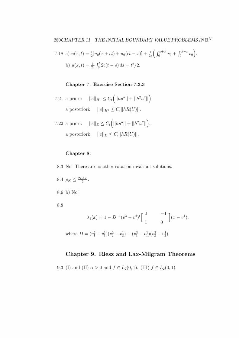
280CHAPTER 11. THE INITIAL BOUNDARYVALUE PROBLEMS IN RN
7.18 a) u(x, t) = 12[u0(x+ ct) + u0(ct− x)] + 1
2c
( ∫ x+ct
0v0 +
∫ ct−x
0v0
).
b) u(x, t) = 12c
∫ t
02c(t− s) ds = t2/2.
Chapter 7. Exercise Section 7.3.3
7.21 a priori: ||e||H1 ≤ Ci
(||hu′′||+ ||h2u′′||
).
a posteriori: ||e||H1 ≤ Ci||hR(U)||.
7.22 a priori: ||e||E ≤ Ci
(||hu′′||+ ||h2u′′||
).
a posteriori: ||e||E ≤ Ci||hR(U)||.
Chapter 8.
8.3 No! There are no other rotation invariant solutions.
8.4 ρK ≤ τKhK
2.
8.6 b) No!
8.8
λ1(x) = 1−D−1(v3 − v2)t[ 0 −1
1 0
](x− v1),
where D = (v21 − v11)(v22 − v12)− (v31 − v11)(v
32 − v12).
Chapter 9. Riesz and Lax-Milgram Theorems
9.3 (I) and (II) α > 0 and f ∈ L2(0, 1). (III) f ∈ L2(0, 1).
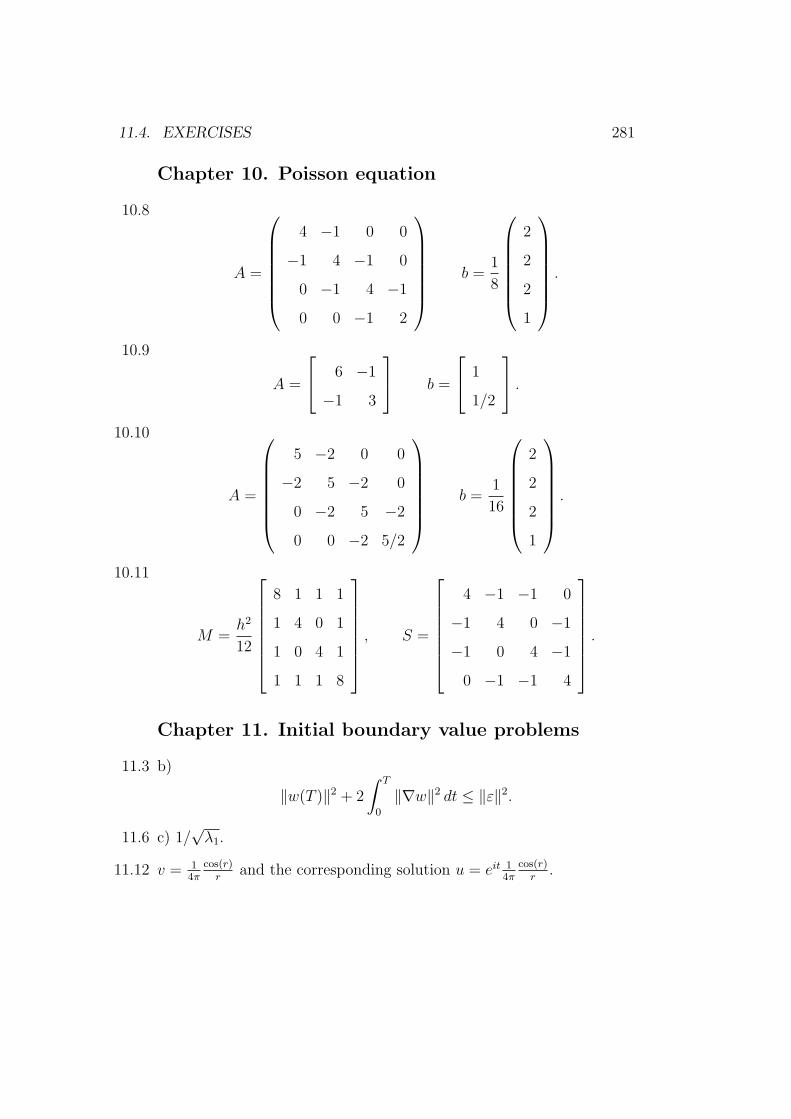
11.4. EXERCISES 281
Chapter 10. Poisson equation
10.8
A =
4 −1 0 0
−1 4 −1 0
0 −1 4 −1
0 0 −1 2
b =1
8
2
2
2
1
.
10.9
A =
6 −1
−1 3
b =
1
1/2
.
10.10
A =
5 −2 0 0
−2 5 −2 0
0 −2 5 −2
0 0 −2 5/2
b =1
16
2
2
2
1
.
10.11
M =h2
12
8 1 1 1
1 4 0 1
1 0 4 1
1 1 1 8
, S =
4 −1 −1 0
−1 4 0 −1
−1 0 4 −1
0 −1 −1 4
.
Chapter 11. Initial boundary value problems
11.3 b)
‖w(T )‖2 + 2
∫ T
0
‖∇w‖2 dt ≤ ‖ε‖2.
11.6 c) 1/√λ1.
11.12 v = 14π
cos(r)r
and the corresponding solution u = eit 14π
cos(r)r
.

282CHAPTER 11. THE INITIAL BOUNDARYVALUE PROBLEMS IN RN

Chapter 12
Algorithms and MATLABCodes
To streamline the computational aspects, we have gathered suggestions forsome algorithms and Matlab codes that can be used in implementations.These are simple specific Matlab codes on the concepts such as
• The L2-projection.
• Numerical integration rules: Midpoint, Trapezoidal, Simpson.
• Finite difference Methods: Forward Euler, Backward Euler, Crank-Nicolson.
• Matrices/vectors: Stiffness- Mass-, and Convection Matrices. Load vector.
The Matlab codes are not optimized for speed, but rather intended to be easy toread.
283

284 CHAPTER 12. ALGORITHMS AND MATLAB CODES
An algorithm for L2-projection:
1. Choose a partition Th of the interval I into N sub-intervals, N+1 nodes,and define the corresponding space of piece-wise linear functions Vh.
2. Compute the (N + 1) × (N + 1) mass matrix M and the (N + 1) × 1load vector b, viz
mij =
∫
Iϕjϕi dx, bi =
∫
Ifϕi dx.
3. Solve the linear system of equations
Mξ = b.
4. Set
Phf =
N∑
j=0
ξjϕj .
Below are two versions of Matlab codes for computing the mass matrix M:
function M = MassMatrix(p, phi0, phiN)
%--------------------------------------------------------------------
% Syntax: M = MassMatrix(p, phi0, phiN)
% Purpose: To compute mass matrix M of partition p of an interval
% Data: p - vector containing nodes in the partition
% phi0 - if 1: include basis function at the left endpoint
% if 0: do not include a basis function
% phiN - if 1: include basis function at the right endpoint
% if 0: do not include a basis function
%--------------------------------------------------------------------
N = length(p); % number of rows and columns in M
M = zeros(N, N); % initiate the matrix M

285
% Assemble the full matrix (including basis functions at endpoints)
for i = 1:length(p)-1
h = p(i + 1) - p(i); % length of the current interval
M(i, i) = M(i, i) + h/3;
M(i, i + 1) = M(i, i + 1) + h/6;
M(i + 1, i) = M(i + 1, i) + h/6;
M(i + 1, i + 1) = M(i + 1, i + 1) + h/3;
end
% Remove unnecessary elements for basis functions not included
if ˜phi0
M = M(2:end, 2:end);
end
if ˜phiN
M = M(1:end-1, 1:end-1);
end
A Matlab code to compute the mass matrix M for a non-uniform mesh:
Since now the mesh is not uniform (the sub-intervals have different lengths), wecompute the mass matrix assembling the local mass matrix computation for eachsub-interval. To this end we can easily compute the mass matrix for the standard
interval I1 = [0, h] with the basis functions ϕ0 = (h − x)/h and ϕ1 = x/h: Then,
1
x0 = 0 x1 = hx
ϕ0(x)ϕ1(x)
Figure 12.1: Standard basis functions ϕ0 = (h− x)/h and ϕ1 = x/h.

286 CHAPTER 12. ALGORITHMS AND MATLAB CODES
the standard mass matrix is given by
M I1 =
∫I1ϕ0ϕ0
∫I1ϕ0ϕ1
∫I1ϕ1ϕ0
∫I1ϕ1ϕ1
.
Inserting for ϕ0 = (h− x)/h and ϕ1 = x/h we compute M I1 as
M I1
∫ h0 (h− x)2/h2 dx
∫ h0 (h− x)x/h2 dx
∫ h0 x(h− x)/h2 dx
∫ h0 x2/h2 dx
=
h
6
2 1
1 2
. (12.0.1)
Thus, for an arbitrary sub-interval Ik := [xk−1, xk] with the mesh size hk, andbasis functions ϕk and ϕk−1 (see Fig. 3.4.), the local mass matrix is given by
M Ik =
∫Ikϕk−1ϕk−1
∫Ikϕk−1ϕk
∫Ikϕkϕk−1
∫Ikϕk1ϕk
=
hk6
2 1
1 2
(12.0.2)
where hk is the length of the interval Ik. Note that, assembling, the diagonalelements in the Global mass matrix will be multiplied by 2 (see Example 4.1).These elements are corresponding to the interior nodes and are the result of addingtheir contribution for the intervals in their left and right. The assembling is throughthe following Matlab routine:
A Matlab routine to compute the load vector b:
To solve the problem of the L2-projection, it remains to compute/assemble theload vector b. To this end we note that b depends on the unknown function f ,and therefore will be computed by some of numerical integration rules (midpoint,trapezoidal, Simpson or general quadrature). Below we shall introduce Matlabroutines for these numerical integration methods.
function b = LoadVector(f, p, phi0, phiN)
%--------------------------------------------------------------------
% Syntax: b = LoadVector(f, p, phi0, phiN)
% Purpose: To compute load vector b of load f over partition p
% of an interval
% Data: f - right hand side funcion of one variable
% p - vector containing nodes in the partition

287
% phi0 - if 1: include basis function at the left endpoint
% if 0: do not include a basis function
% phiN - if 1: include basis function at the right endpoint
% if 0: do not include a basis function
%--------------------------------------------------------------------
N = length(p); % number of rows in b
b = zeros(N, 1); % initiate the matrix S
% Assemble the load vector (including basis functions at both endpoints)
for i = 1:length(p)-1
h = p(i + 1) - p(i); % length of the current interval
b(i) = b(i) + .5*h*f(p(i));
b(i + 1) = b(i + 1) + .5*h*f(p(i + 1));
end
% Remove unnecessary elements for basis functions not included
if ˜phi0
b = b(2:end);
end
if ˜phiN
b = b(1:end-1);
end
The data function f can be either inserted as f=@(x) followed by some expressionin the variable x, or more systematically through a separate routine, here called“Myfunction” as in the following example
Example 12.1 (Calling a data function f(x) = x2 of the load vector).function y= Myfunction (p)
y=x.ˆ2
\vskip 0.3cm
Then, we assemble the corresponding load vector, viz:
\beginverbatim
b = LoadVector (@Myfunction, p, 1, 1)

288 CHAPTER 12. ALGORITHMS AND MATLAB CODES
Alternatively we may write
f=@(x)x.ˆ2
b = LoadVector(f, p, 1, 1)
Now we are prepared to write a Matlab routine “My1DL2Projection” for computing
the L2-projection.
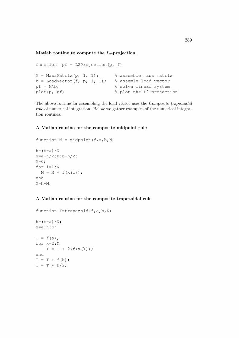
289
Matlab routine to compute the L2-projection:
function pf = L2Projection(p, f)
M = MassMatrix(p, 1, 1); % assemble mass matrix
b = LoadVector(f, p, 1, 1); % assemle load vector
pf = M\b; % solve linear system
plot(p, pf) % plot the L2-projection
The above routine for assembling the load vector uses the Composite trapezoidal
rule of numerical integration. Below we gather examples of the numerical integra-tion routines:
A Matlab routine for the composite midpoint rule
function M = midpoint(f,a,b,N)
h=(b-a)/N
x=a+h/2:h:b-h/2;
M=0;
for i=1:N
M = M + f(x(i));
end
M=h*M;
A Matlab routine for the composite trapezoidal rule
function T=trapezoid(f,a,b,N)
h=(b-a)/N;
x=a:h:b;
T = f(a);
for k=2:N
T = T + 2*f(x(k));
end
T = T + f(b);
T = T * h/2;

290 CHAPTER 12. ALGORITHMS AND MATLAB CODES
A Matlab routine for the composite Simpson’s rule
function S = simpson(a,b,N,f)
h=(b-a)/(2*N);
x = a:h:b;
p = 0;
q = 0;
for i = 2:2:2*N % Define the terms to be multiplied by 4
p = p + f(x(i));
end
for i = 3:2:2*N-1 % Define the terms to be multiplied by 2
q = q + f(x(i));
end
S = (h/3)*(f(a) + 2*q + 4*p + f(b)); % Calculate final output
The precomputations for standard and local stiffness and convection matrices:
SI1 =
∫I1ϕ′0ϕ
′0
∫I1ϕ′0ϕ
′1
∫I1ϕ′1ϕ
′0
∫I1ϕ1′ϕ′
1
=
∫I1
−1h
−1h
∫I1
−1h
1h∫
I11h−1h
∫I1
1h1h
=
1
h
1 −1
−1 1
.
As in the assembling of the mass-matrix, even here, for the global stiffness matrix,each interior node has contributions from both intervals that the node belongs.Consequently, assembling we have 2/h as the interior diagonal elements in thestiffness matrix (rather than 1/h in the single interval computes above). For theconvection matrix C, however, because of the skew-symmetry the contributionsfrom the two adjacent interior intervals will cancel out:
CI1 =
∫I1ϕ′0ϕ0
∫I1ϕ0ϕ
′1
∫I1ϕ1ϕ
′0
∫I1ϕ1′ϕ1
=
∫I1
−1h
h−xh
∫I1
h−xh
1h∫
I1xh−1h
∫I1
xh1h
=1
2
−1 1
−1 1
.
A thorough computation of all matrix elements, for both interior and bound-ary nodes, in the case of continuous piece-wise linear approximation, for Mass-,stiffness- and convection-matrices are demonstrated in Examples 4.1 and 4.2.

291
A Matlab routine assembling the stiffness matrix:
function S = StiffnessMatrix(p, phi0, phiN)
%---------------------------------------------------------------------
% Syntax: S = StiffnessMatrix(p, phi0, phiN)
% Purpose: To compute the stiffness matrix S of a partition p of an
% interval
% Data: p - vector containing nodes in the partition
% phi0 - if 1: include basis function at the left endpoint
% if 0: do not include a basis function
% phiN - if 1: include basis function at the right endpoint
% if 0: do not include a basis function
%---------------------------------------------------------------------
N = length(p); % number of rows and columns in S
S = zeros(N, N); % initiate the matrix S
% Assemble the full matrix (including basis functions at endpoints)
for i = 1:length(p)-1
h = p(i + 1) - p(i); % length of the current interval
S(i, i) = S(i, i) + 1/h;
S(i, i + 1) = S(i, i + 1) - 1/h;
S(i + 1, i) = S(i + 1, i) - 1/h;
S(i + 1, i + 1) = S(i + 1, i + 1) + 1/h;
end
% Remove unnecessary elements for basis functions not included
if ˜phi0
S = S(2:end, 2:end);
end
if ˜phiN
S = S(1:end-1, 1:end-1);
end

292 CHAPTER 12. ALGORITHMS AND MATLAB CODES
A Matlab routine to assemble the convection matrix:
function C = ConvectionMatrix(p, phi0, phiN)
%--------------------------------------------------------------------------
% Syntax: C = ConvectionMatrix(p, phi0, phiN)
% Purpose: To compute the convection matrix C of a partition p of an
% interval
% Data: p - vector containing nodes in the partition
% phi0 - if 1: include a basis function at the left endpoint
% if 0: do not include a basis function
% phiN - if 1: include a basis function at the right endpoint
% if 0: do not include a basis function
%--------------------------------------------------------------------------
N = length(p); % number of rows and columns in C
C = zeros(N, N); % initiate the matrix C
% Assemble the full matrix (including basis functions at both endpoints)
for i = 1:length(p)-1
C(i, i) = C(i, i) - 1/2;
C(i, i + 1) = C(i, i + 1) + 1/2;
C(i + 1, i) = C(i + 1, i) - 1/2;
C(i + 1, i + 1) = C(i + 1, i + 1) + 1/2;
end
% Remove unnecessary elementC for basis functions not included
if ˜phi0
C = C(2:end, 2:end);
end
if ˜phiN
C = C(1:end-1, 1:end-1);
end

293
Finally, below we gather the Matlab routines for finite difference approximations(also cG(1) and dG(0) ) for the time discretizations.
Matlab routine for Forward-, Backward-Euler and Crank-Nicolson:
function [] = three_methods(u0, T, dt, a, f, exactexists, u)
% Solves the equation du/dt + a(t)*u = f(t)
% u0: initial value; T: final time; dt: time step size
% exactexists = 1 <=> exact solution is known
% exactexists = 0 <=> exact solution is unknown
timevector = [0]; % we build up a vector of
% the discrete time levels
U_explicit_E = [u0]; % vector which will contain the
% solution obtained using "Forward Euler"
U_implicit_E = [u0]; % vector which will contain the
% solution with "Backward Euler"
U_CN = [u0]; % vector which will contain the
% solution using "Crank-Nicolson"
n = 1; % current time interval
t_l = 0; % left end point of the current
% time interval, i.e. t_n-1
while t_l < T
t_r = n*dt; % right end point of the current
% time interval, i.e. t_n
% Forward Euler:
U_v = U_explicit_E(n); % U_v = U_n-1
U_h = (1-dt*a(t_l))*U_v+dt*f(t_l); % U_h = U_n;
U_explicit_E(n+1) = U_h;

294 CHAPTER 12. ALGORITHMS AND MATLAB CODES
% Backward Euler:
U_v = U_implicit_E(n); % U_v = U_n-1
U_h = (U_v + dt*f(t_r))/(1 + dt*a(t_r)); % U_h = U_n
U_implicit_E(n+1) = U_h;
% Crank-Nicolson:
U_v = U_CN(n); % U_v = U_n-1
U_h = ((1 - dt/2*a(t_l))*U_v + dt/2*(f(t_l)+f(t_r))) ...
/ (1 + dt/2*a(t_r)); % U_h = U_n
U_CN(n+1) = U_h;
timevector(n+1) = t_r;
t_l = t_r; % right end-point in the current time interval
% becomes the left end-point in the next time interval.
n = n + 1;
end
% plot (real part (in case the solutions become complex))
figure(1)
plot(timevector, real(U_explicit_E), ’:’)
hold on
plot(timevector, real(U_implicit_E), ’--’)
plot(timevector, real(U_CN), ’-.’)
if (exactexists)
% if known, plot also the exact solution
u_exact = u(timevector);
plot(timevector, real(u_exact), ’g’)
end
xlabel(’t’)
legend(’Explicit Euler’, ’Implicit Euler’, ’Crank-Nicolson’, 0)
hold off

295
if (exactexists)
% if the exact solution is known, then plot the error:
figure(2)
plot(timevector, real(u_exact - U_explicit_E), ’:’)
hold on
plot(timevector, real(u_exact - U_implicit_E), ’--’)
plot(timevector, real(u_exact - U_CN), ’-.’)
legend(’Explicit Euler’, ’Implicit Euler’, ’Crank-Nicolson’, 0)
title(’Error’)
xlabel(’t’)
hold off
end
return
Example 12.2. Solving u′(t) + u(t) = 0 with three_methods
a= @(t) 1;
f= @(t) 0;
u= @(t) exp(-t)
u_0=1;
T= 1;
dt=0.01;
three_methods (u_0, T, dt, a, f, 1, u)

296 CHAPTER 12. ALGORITHMS AND MATLAB CODES

Bibliography
[1] V. I. Arnold, Ordinary differential Equations, (Translated from theRussian by Richard A. Silverman), MIT Press, Cambridge, Mas-sachusetts, and London, England, 2en Ed. 1980.
[2] M. Asadzadeh, Analys och Linjar Algebra, Studentlitteratur, 2007. pp432.
[3] M. Asadzadeh, Lecture Notes in Fourier Analysis, (Electronic availablein author’s website), pp 342.
[4] M. Asadzadeh, Lecture Notes in Finite Element Methods for Partial
Differential Equations, Compendium, 2011, Chalmers Univ of Tech.2nd edition. (also available online in author’s website), pp 326.
[5] K. Atkinson, An Introduction to Numerical Analysis, 2ed Ed. JohnWiley & Sons, Inc, New York, 1989.
[6] J. Axler, Linear Algebra Done Right, Springer Verlag, 1997.
[7] F. Bengzon and M. Larson, The Finite Element Method: Theory, Im-
plementation and practice. Springer 2013.
[8] K. Bohmer, Numerical Methods for Nonlinear Elliptic Differential
Equations, Oxford University Press, 2010.
[9] D. Braess, Finite Elements. Theory, fast solvers, and application insolid mechanics, 2ed Ed. Cambridge Universityu Press, 2001.
[10] S. Brenner and L. R. Scott, The Mathematical Theory of Finite Ele-
ment Methods, Springer-Verlag, New York, 1994.
[11] L. R. Burden and J. D. Faires, Numerical Analysis, Fifth Ed.Brook/Cole, CA, 1998.
297

298 BIBLIOGRAPHY
[12] J. C. Butcher, Numerical Methods for Ordinary Differential Equations,John Wiley, 2nd edition, 2008.
[13] E. W. Cheney, Introduction to Approximation Theory. AmericanMathematical Society, Providence, RI, 2nd edition, 2000.
[14] P. Ciarlet, The Finite Element Method for Elliptic Problems, North-Holland, New York, 1980.
[15] [10] P. Ciarlet, Introduction to Matrix Numerical Analysis and Opti-
mization (in French), Masson, Paris, 1982.
[16] G. Dahlquist and A. Bjork, Numerical Methods, Dover, 2003.
[17] P. Davis and P. Rabinowitz, Methods of Numerical Integration, Aca-demic Press, 2nd edition, 1984.
[18] J. W. Demmel, Applied Numerical Linear Algebra, Society for Indus-trial and Applied Mathematics, Philadelphia, PA, 1997.
[19] A. Ern and J. -L. Guermond, Theory and Practice of Finite Elements,Applied Mathematical Sciences, Springer Verlag, 2004.
[20] K. Eriksson, D. Estep, P. Hansbo and C. Johnson, Computational
Differential Equations, Studentlitteratur, Lund, 1996.
[21] L. C. Evans, Partial Differential Equations, Graduate Studies in Math-ematics, 19. Americam Mathematical Society, Providance, RI, 1998.
[22] G. B. Folland, Fourier Analysis and its Applications, Waswoth & Cole1992.
[23] G. B. Folland, Intorduction to Partial Differential Equations, PrincetonUniversity Press, 1976.
[24] G. Golub and C. V. Loan, Matrix Computations, John Hopkins Uni-versity Press, Maryland, 1983.
[25] K. E. Gustafson, Partial Differential Equations and Hilbert Space
Methods, John Wiley & Sons, New York, 1980.
[26] M. Guterman and Z. Nitecki, Differential Equations: A first Course,Third Ed, Saunders College Publishing, 1992.
[27] P. Henrici, Elements of Numerical Analysis. Mc Graw Hill, 1953.

BIBLIOGRAPHY 299
[28] A. S. Houiseholder, Principles of Numerical Analysis. John Wiley, 1964.
[29] T. J. R. Hughes, The Finite Element Method. Linear Static and Dy-namic Finite Element Analysis, Prentice-Hall, Englewood Cliffs, NewJersy, 1987.
[30] E. Isaacson and H. B. Keller, Analysis of Numerical Methiods. Dover,1994.
[31] C. Johnson, Numerical Solutions of Partial Differential Equations by
the Finite Element Method, Studentlitteratur, Lund, 1991.
[32] V. I. Krylov, Approximate Calculation of Integrals. Macmillan Press,1962.
[33] S. Larsson and V. Thomee, Partial differential equations with nu-
merical methods. Texts in Applied Mathematics, 45. Springer-Verlag,Berlin, 2003.
[34] N. Lebovitz, Ordinary Differential Equations. Brooks/Cole, 2002.
[35] A. Logg, K-A. Mardal and G. N. Wells, eds. Automated Solution of
Differential Equations by the Finite Element Method. Springer 2012.
[36] G. C. Lorentz, Approximation of Functions. Chelsea, New York, 2ndedition, 1986.
[37] R. Kent Nagle and Edward B. Saff, Differential Equations and Bound-
ary Value Problems, Assison Weseley, 1993.
[38] J. T. Oden, Finite elements: an introduction. Handbook of numeri-cal analysis, Vol. II, 3–15, Handb. Numer. Anal., II, North-Holland,Amsterdam, 1991.
[39] J. T. Oden and L. F. Demkowicz, Applied Functional Analysis. CRCPress, 1996.
[40] A. M. Ostrowski, Solution of Equations and Systems of Equations.
Academic Press, 1966.
[41] B. Parlett, Very early days of matrix computations. SIAM News, 36(9),2003.
[42] M. J. D. Powell, Apprximation Theory and Methods. Cambridge Uni-versity Press, 1981.

300 BIBLIOGRAPHY
[43] J. R. Rice, The Approximation of Functions, Volume 1. Addison-Wesely, 1969.
[44] J. R. Rice, The Approximation of Functions, Volume 2. Addison-Wesely, 1969.
[45] W. Rudin, Priciples of Mathematical Analysis. Mc Graw-Hill, 3rdedirion, 1976.
[46] L. Ridgway Scott, Numerical Amalysis, Princeton, 2011.
[47] G. W. Stewart, Matrix Algorithms, Volume 1: Basic Decompositions.
Philadelphi: Society for Industrial and Applied Mathematics, 1998.
[48] G. W. Stewart, Matrix Algorithms, Volume II: Eigenvalue Problems.
Philadelphi: Society for Industrial and Applied Mathematics, 2001.
[49] G. Strang, Introduction to Applied Mathematics, Wellesely-CambridgePress, Cambridge, Mass, 1986.
[50] G. Strang, and G. J. Fix, An analysis of the finite element method.
Prentice-Hall Series in Automatic Computation. Prentice-Hall, Inc.,Englewood Cliffs, N. J., 1973.
[51] W. Strauss, Partial Differential Equations. An Introduction, 2ed Ed.John Wiley & Sons, Ltd, 2008.
[52] M. E. Taylor, Partial Differential Equations. I. Basic Theory. AppliedMathematical Sciences, 115. Springer-Verlag, New York, 1996.
[53] V. Thomee, Galerkin Finite Element Methods for Parabolic Prob-
lems, Lecture Notes in Mathematics 1054. Springer-Verlag, New York,Tokyo, 1984.
[54] Lloyd N. Trefethen and David Bau, III. Numerical Linear Algebra. So-ciety for Industrial and Applied Mathematics, Philadelphia, PA, 1997.
[55] Richard S. Verga, Matrix Interative Analysis. Springer, 2nd edition,2000.
[56] J. H. Wilkinson, The algebraic Eigenvalue Problem, Oxford, 1995.
[57] S. Yakowitz and F. Szidarovsky, An Introduction to Numerical Com-
putations, 2ed Ed. Macmillan Co. New York, 1989.
[58] O. C. Zienkiewicz, The Finite Element Method in Structural and Con-
tinum Mechanics. McGraw-Hill, London, 1971.

BIBLIOGRAPHY 301
Table of Symbols
Symbol reads Exempel/Definition
∀ for all, for every ∀x, cos2 x+ sin2 x = 1
∃ There exists There exists x ∈ R such that x+ 1 > 4 (example x ∈ R and x > 3)
: such that ∃x : x > 3
∨ or x ∨ y (x or y)
∧ or & and x ∧ y (x and y) also x & y
∈ belongs√2 ∈ R (
√2 is a real numbers R)
/∈ not belongs√2 /∈ Q (
√2 is not a rational number )
⊥ orthogonal to u ⊥ v (u and v are orthogonal)
:= defines as I :=
∫ b
a
f(x) dx (I defines as integralen in RHS)
=: defines
∫ b
a
f(x) dx =: I (The integral in LHS defines I)
≈ approximates A ≈ B (A approximates B) or A is approximately equal to B.
=⇒ implies A =⇒ B (A implies B.)
⇐⇒ equivalent A⇐⇒ B (A is equivalent to B.)
ODE Ordinary Differential Equation
PDE Partial Differential Equation
IVP Initial Value Problem
BVP Boundart Value Problem
VF Variational Formulation
MP Minimization Problem
Pq(I) p ∈ Pq(I) p(x) is a polynomial of degree ≤ q for x ∈ I.
H1(I) v ∈ H1(I) if
∫ b
a
(v(x)2 + v′(x)2
)dx <∞, I = [a, b].
Vh(I) v ∈ Vh(I) the space of piecewise linear functions on a partition of I.
V 0h (I) v ∈ V 0
h (I) v ∈ Vh(I) and v is 0 at both or one of the boundary points.

302 BIBLIOGRAPHY
Symbol reads Exempel/Definition
||f ||p, ||f ||Lp(I) Lp-norm of f on I ||f ||p :=
(∫
I
|f(x)|p dx)1/p
, 1 ≤ p <∞
maxx∈I |f(x)|, p = ∞
Lp(I) Lp-space f ∈ Lp(I) iff ||f ||p <∞
||v||a weighted L2-norm ||v||a :=(∫
I
a(x)|v(x)|2 dx)1/2
, a(x) > 0
||v||E the energy norm ||v||E :=(∫
I
a(x)|v(x)′|2 dx)1/2
, ||v||E = ||v′||a.
∏product
N∏
i=1
i = 1 · 2 · 3 · . . . ·N =: N !
∑sum
N∑
i=1
i = 1 + 2 + 3 + . . .+N =: N(N + 1)/2
(u, v) or 〈u, v〉 skalar/inner product(u, v) := u1v1 + u2v2 + . . .+ uNvN , u, v ∈ RN
(u, v) :=
∫
I
u(x)v(x) dx for u, v ∈ L2(I).
Phf L2-projection (f, w) = (Phf, w), ∀w ∈ Pq(a, b).
Th(I) a partition of I Th[a, b] : a = x0 < x1 < . . . < xN = b.
πhf interpolant of f πhf(xi) = f(xi) in a partition Th of I = [a, b].
FDM Finite Difference Method
FE Forward Euler Forward Euler FDM
BE Backward Euler Backward Euler FDM ⇐⇒ dG(0)
CN Crank-Nicolson Crank-Nicolson FDM ⇐⇒ cG(1)
FEM Finite Element Metthod/Galerkin Method
cG(1) continuous Galerkin continuous, piecewise linear Galerkin approx
dG(0) discont. Galerkin discontinuous, piecewise constant Galerkin
cG(1)cG(1) continuous Galerkin space time continuous, piecewise linear Galerkin
Ci Interpolation Constant
Cs Stability constant
TOL Error TOLerance

Index
A
Adaptivity 125, 157, 190, 249
B
boundary condition 12-13, 18, 21, 22,
25, 26, 51, 55, 56, 116-118, 174,
176, 197, 219, 223, 244, 270
Dirichlet 14, 36, 50, 118, 126, 181,
191, 215
essential 118,
mixed 116, 175, 255,
natural 118,
Neumann 14, 36, 118, 191, 261
Robin 14, 118, 195, 273.
Boundary value problem 12, 17, 36, 41,
57, 59, 111, 114, 119, 126, 141,
203, 215, 218, 227, 257,
Two point bvp 25, 55, 111, 117
C
Cauchy-Schwarz 43, 49, 121, 124, 176,
177, 236, 237, 238
Conservation of energy 24-27, 194-195,
199, 269, 273
Convection 26, 126, 133-134, 195,
201, 202, 204, 206, 207, -129
Convection-diffusion 34, 126, 131, 173,
201, 202, 203, 208, 237,
Convection matrix 133, 292, 294
Crank-Nicolson 148, 170, 183, 272, 285,
295, 296, 297, 304
D
differential equation 7-13, 16, 18, 20,
21, 22, 23, 25, 35, 56, 58, 73,
73, 89, 117, 118, 146, 176, 179,
303

304 BIBLIOGRAPHY
180, 195, 214, 215, 218, 236,
ordinary differential equation 7-9, 14,
18, 35, 141
partial differential equation 7, 8, 12,
17, 18, 23, 36, 174,
linear 20-22,
nonlinear 19,
quasilinear 19,
differential operator 9, 19, 20, 23,
89, 195
linear 9,
Diffusion 9, 11, 26, 28, 131, 195,
201, 206, 258,
E
Error estimates 7, 63, 65, 72, 86, 120,
151, 154, 161, 162, 166, 173,
191, 221, 223, 245, 257,
a posteriori 7, 111, 120,
123, 125, 139, 140, 148,
169, 186, 187, 190, 243, 250-251
a priori 7, 111, 120, 122, 148,
149, 158, 159, 160, 171, 193,
246-250, 254, 264, 272, 273
Interpolation error 72, 73, 86, 151,
221, 225,
Error representation formula 150, 151,
154-156, 163, 165, 163, 165
Euler scheme 147,
Existence 7, 15, 18, 231, 236, 237
F
Finite dimensional spaces 8, 38, 45, 50,
70, 89, 119, 126, 245, 254,
Finite Element Method 7, 18, 35, 38,
41, 45, 51, 89, 119, 136, 137, 139
141, 143, 181, 185, 197, 203,
217, 243, 245, 257, 262,
Continuous Galerkin 119, 126, 144
146, 218,
Disontinuous Galerkin 144, 146, 183,
186, 201,
Fundamental solution 16, 258
G
Galerkin Method IVP 144, 146, 171

BIBLIOGRAPHY 305
Galerkin Method BVP 49, 218,, 102
Galerkin Method IBVP 181
Gauss elimination 90, 92, 94, 96, 99
Gauss quadrature 58, 80, 81, 82
Gauss-Seidel 58, 101-104, 106-108,
H
hat function 41, 60, 66, 113, 119,
126, 127, 132, 181, 217,
half hat function 66, 117,
Heat equation 10-12, 23-26, 28, 36,
49, 55, 126, 173-175, 178-179
181, 186, 257-259, 264
I
Interpolation
Lagrange interpolation 67-75
83, 191,
linear interpolation 61-65, 84,
221
polynomial interpolation 38,
Initial Boundary Value Problem (IBVP)
36, 141, 173, 175, 178, 194,
257, 258, 268,
Initial value problem 11, 34, 35, 44, 57,
141, 144, 148, 168, 196,
J, K
Jacobi method 99, 100, 103
L
Lagrange basis 38-40, 64, 68-71, 82
Linear equation system 13, 100,
linear space 38, 42, 231
L2-projection 47-48, 51, 150, 162, 285,
M
Mass Matrix 129, 130, 183-185,
219, 263, 286-288
positive definite 57, 97, 228, 263
Minimization problem 111, 114-115, 135,
Mixed bvp 116,
N
Neumann problem/data 240, 244,
Numerical integration 7, 61, 73, 285,
288, 291
306 BIBLIOGRAPHY
Composite midpoint 58, 77, 79, 291
Composite trapezoidal 77, 80, 291
Composite Simpson’s 78, 79, 80, 292
Simple midpoint 74, 79,
Simple trapezoidal 74, 79,
Simple Simpson’s 75, 80,
Norm 43
L2-norm 43, 49, 63, 120, 125, 176,
246, 259, 260
Lp-norm 63, 65, 120, 221
vector norm 63
maximum norm 63, 65, 98, 101, 120,
221
energy norm 120, 121, 123, 229, 259,
272
weighted norm 120, 122
O
Ordinary Differential Equations
(ODE) 7-9, 18, 35 , 141
Orthogonality 43, 45, 151, 153-154
Order of a differential equation
8, 13, 18
P
Partial Differential Equations
(PDE) 7-8, 17, 18, 20, 23, 36, 174
elliptic 10-11,
homogeneous 8, 20-22, 25, 175, 179
hyperbolic 10-11,
inhomogeneous 8-9, 21, 24, 26, 32,
50, 55-56, 126
Laplace 9, 12, 24, 29, 257,
parabolic 10-11,
Poisson equation 23, 111, 190, 236,
243
potential equation 10-11,
Tricomi equation 10,
partition 37, 40, 47, 50, 66, 67, 73, 76
119, 127, 131, 145, 181, 197
214, 286
Poincare inequality 175, 177, 192, 211,

BIBLIOGRAPHY 307
232
Q
R
Residual 44-45, 120, 123, 146, 155, 187,
S
Scalar initial value problem, 141,
Scalar product 42-43, 62-63, 229-231,
S.O.R. 104
stability 15, 19, 142, 173, 178, 205, 243,
259,
stability estimate 173, 175, 180, 189,
stability factor 150, 160, 164, 168,
strong stability 250, 251,
weak stability 244,
Stiffness matrix, 52-54, 56, 128, 133,
183, 219-220, 263, 271, 292
Streamline-Diffusion 201, 206,
Superposition 19, 21-22.
T
Taylor expansion 64, 66, 71, 72
test function 16, 44-46, 50, 112, 118,
127, 131-132, 144, 206,
trial function 45, 50, 119, 126, 131, 146,
U
V/W
Variational formulation 44, 50, 112,
181, 196, 211, 219, 227, 245, 262,
wave equation 10, 12, 23, 29, 32,
194-196, 269, 271, 272,
Well-posed problem 18-19,
XYZ