An Object Oriented Shared Data Model for GIS and Distributed Hydrologic Models

M. Kumar and C. Duffy

International Journal of Geographical Information Science, IJGIS-2008-0131

Accepted for publication Sep. 2008

Abstract Distributed physical models for the space-time distribution of water, energy, vegetation, and mass flow require new strategies for data representation, model domain decomposition, a-priori parameterization, and visualization. The Geographic Information System (GIS) has been traditionally used to accomplish these data management functionalities in hydrologic applications. However, the interaction between the data management tools and the physical model are often loosely integrated and nondynamic. This leads to several issues addressed in this paper: a) The data types and formats for the physical model system and the distributed data or parameters may be different, with significant data preprocessing required before they can be shared. b) The management tools may not be accessible or shared by the GIS and physical model. c) The individual systems may be operating-system dependent or are driven by proprietary data structures. The impediment to seamless data flow between the two software components has the effect of increasing the model setup time and analysis time of model output results, and also makes it restrictive to perform sophisticated numerical modeling procedures (sensitivity analysis, real time forecasting, etc.) that utilize extensive GIS data. These limitations can be offset to a large degree by developing an integrated software component that shares data between the (hydrologic) model and the GIS modules. We contend that the pre-requisite for the development of such an integrated software component is a “shared data-model” that is designed using an Object Oriented Strategy. Here we present the design of such a shared data model taking into consideration the data type descriptions, identification of data-classes, relationships and constraints. The developed data model has been used as a method base for developing a coupled GIS interface to Penn State Integrated Hydrologic Model (PIHM) called PIHMgis. 1. Introduction

Physics-based distributed hydrologic models (DHMs) simulate hydrologic state variables in space and time while using information regarding heterogeneity in climate, land use, topography and hydrogeology (Freeze and Harland 1969; Kollet and Maxwell 2006). Because of the large number of physical parameters incorporated in the model, intensive data development and assignment is needed for accurate and efficient model simulations. A Geographic Information System (GIS) has the ability to handle both spatial and non-spatial data, and to perform data management and analysis. However it lacks the sophisticated analytical and modeling capabilities (Maidment 1993; Wilson 1996; Abel et. al. 1994 and Kopp 1996). On the other hand from the physical model perspective, they generally lack data organization and development functionalities. Moreover, the data structure they are based on doesn’t facilitate close linkage to the GIS and decision support system (DSS) (National Research Council 1999). This increases the model setup time, hinders analysis of model output results, compounds data isolation, reduces data integrity and limits concurrent access of data because of broken data flow between the data, physical model, and decision support systems. The problem is acute when dynamic interaction is required during the model simulation. A need for restructuring of individual GIS and physical-modeling systems provides the motivation for this paper.

One important effort in bridging the gap between hydrologic model and GIS is due to Smith and Maidment (1995), who developed a Hydrologic Data Development System (HDDS) based on ARC/INFO. Other instances of development of interfaces for modeling are water and erosion prediction project (WEPP) interface on GRASS (Engel et. al. 1993), an interface between ArcInfo and HEC modeling system (Hellweger and Maidment 1999), BASINS by EPA (Lahlou et. al. 1998), SWAT by Luzio et. al.(2002) , inland waterway contaminant spills modeling interface (Martin et. al. 2004) and Watershed Modeling System (WMS, Nelson 1997). An overview of attempts to develop hydrologic models inside GIS are reviewed by Wilson (1999). We note that all the above approaches were basically trying to “couple” a GIS and a process-based hydrologic model for efficient processing, storing, manipulating, and displaying of hydrogeological data. WMS was a major development and different from other attempts in that it was a stand-alone GIS system totally dedicated to hydrologic application. Development of Arc Hydro (Maidment 2002) was another important step in defining an exhaustive data model for a hydrologic system and providing a framework for storing and preprocessing geospatial and temporal data in GIS. The developed data model provided rules for the structure, relationships and operations on data types often used in hydrologic modeling. McKinney and Cai (2002) went a step further in reducing the gap between GIS and models by outlining an object oriented methodology to link GIS and water management models. In the process, they identified the Methods and Objects of the water management models that can be represented as spatial and thematic characteristic in the GIS.

In this paper we propose a robust integration methodology that facilitates seamless data flow between data and model functionalities thus making the interactions between them fluid and dynamic. The objective of this work is to lay the foundation for fully integrated and extensible, GIS-DHM system through a shared data model that can support both of them. The shared data model provides a) flexibility of modification and customization b) ease of access of GIS data structure by the hydrologic model c) richness for representing complex user defined spatial relations and data types, and d) standardization easily applicable to new model settings and modeling goals. The data model has been developed using state of the art computer programming concepts of object oriented programming (OOP). We also discuss in detail the intermediate steps of designing the shared data model from a GIS data model. The emphasis in this exercise is elucidating program design, not the coding details. The resulting data model supports a coupled framework that serves as a GIS interface to Pennstate Integrated Hydrologic Model (PIHM) and is called PIHMgis. PIHMgis is developed on the QGIS open source framework. The strategy presented here shows that the concepts and capabilities unique to the physical coupling approach can easily be implemented in other GIS’s and DHM’s. An example of the integrated software proposed here has been developed using object oriented programming languages like Qt and C++ and is open source (http://sourceforge.net/projects/pihmgis/ ). 2. Integration methodology Efforts to couple GIS with hydrological models (see Table 1) generally follows either a loose, tight, or embedded coupling (Nyerges 1993; Goodchild 1992) strategy. Watkins et. al., (1996) and Paniconi et. al.,(1999) have discussed in detail the relative advantages and

disadvantages of coupling in terms of watershed decomposition, sensitivity and uncertainty analysis, parameter estimation and representation of the watershed. Loose coupling is prone to data inconsistency, information loss and redundancy, leading to increased model setup time. At the same time, loosely coupled approaches are much simpler to design and program. At the other extreme, embedded coupling can leave the code inertial to change because of its large and complex structure (Goodchild 1992; Fedra 1996). Nonetheless embedded coupling provides the dynamic ability to visualize and suspend ongoing simulations, query intermediate results, investigate key spatial/temporal relations, and even modify the underlying hydrologic model parameters (Bennett 1997).

From our point of view both tight and embedded coupling strategies offer the necessary degree of sharing between GIS and hydrologic model for efficient data query, storage, transfer and retrieval. We also note (from Table 1) that both coupling strategies underscore the existence of a shared data model in their implementation. Clearly, the integration of GIS tools and simulation models should first address the conceptual need of a shared data model that is implemented on top of a common data and method base. In order to design such a shared data model, we follow a four-step approach. First we carry out identification and classification of the various data types that form the hydrologic system (section 3). Then we design the object oriented data model for the data types identified in the previous step (section 4). In the third step, we study the hydrologic model structure in terms of its data needs and adjacency relationships (section 5). Finally, re-representation of the GIS-data data model classes to conform to the distributed hydrologic model data structure is carried out (section 6). Next we discuss in detail the design steps of the shared data model. 3. Conceptual classification of raw hydrologic data A hydrologic model domain encompasses a wide range of hydraulic, hydrologic, climatic and geologic data including topography, rivers, soil, geology, vegetation, land use, weather, observation wells and fractures. A conceptual classification of raw hydrologic data needs to incorporate data of different origins, representation types and scales. Figure 1 illustrates a hierarchical categorization of real data typically required in hydrologic models. The design is intended to incorporate spatially heterogeneous thematic data types along with associated time series data, derived data and attributes. The data types can be defined as field-based and object-based (Goodchild 1992). Field based data define a spatial (or temporal) framework consisting of a set of locations related to each other by (temporal) distance, direction and contiguity (Galton 2001). Object based data are collection of individual entities that are characterized by geometry, topology and non-spatial attribute values (Heuvelink 1998). Spatial information to these entities is explicitly defined either as attributes or as a function of location that is inherent in a point, a line or a polygon. We note that this kind of distinction in GIS features has been traditionally associated with raster and vector data only. However, here we extend the concept of field-data by considering it as a “continuous concept” whose unitary element exists either in space or time with respective entity information attached to it. For example, a unit element of any tessellation, like a grid or a TIN (triangular regular network) has an associated value that defines a property/characteristic magnitude/value

anywhere within the field boundary. Similarly for a time series, there is a value attached to any instant in the time series.

Figure 1 shows further sub-classification of “field” and “object” data types that are relevant to hydrologic modeling. An object consists of points, line and polygons. The fundamental scope of the object sub-data types has been extended, in order to incorporate complex features (made up of multiple simple features) and the dynamic nature of observer and observables. We classify Points as Static and Floating depending on their primary existence in space or time. For example, a static point can be identified by a location at which a time series data such as wind speed is being observed. On the other hand, an example of a Floating point can be a volunteer in a soil moisture measurement field campaign who goes around the field taking soil moisture samples at different locations. In the former case, the observer is fixed in space and is observing state in time while in the latter case a continuous time clock is fixed to the observer while he/she moves around and takes sporadic samples at different locations. Static points have been further subcategorized into Isotropic and Anisotropic points. Anisotropic points are locations whose entity attributes needs information regarding direction and magnitude and possibly magnitude changing with direction (e.g a 2nd rank tensor). An example of an anisotropic property representation at a point is hydraulic conductivity (Freeze and Cherry 1979). Line objects have been sub-categorized into standard 2D and a 3D line. 3D polylines are made up of line segments that exist in three dimensions. For example, an underground pipe network for drainage/waste removals etc. which can change directions/planes in 3D at junctions. Polygon objects have been subcategorized into Static and Floating polygons. Floating polygons are bounded regions whose areas changes in time such as a flooded region or a lake. Field objects have been subclassified into Tessellations (spatial) and Time series (temporal) components. Unitary elements of tessellations define units of spaces with entity information attached to it.

The conceptual representation discussed above is generic and acts as a template that can be populated by new data. Next we try to formally represent the data types in classes and identify their attributes and their relationships with other classes. 4. Hydrologic Data Model Design A hydrologic data model is a formal representation of the real world that provides a standard structure for storage, sharing and exchange of data independent of the software environment and programming languages. It provides a simplified abstraction of reality by a) isolating real world hydrologic objects into independent classes, b) removing redundant class objects, c) defining relationships between independent classes, and d) defining integrity constraints on them.

The design of a hydrologic data model is performed keeping in mind the range of required data types and their relationships among themselves (Wright et. al. 2007). Some data, such as elevation and soil properties, vary continuously in space while others like observed streamflow vary continuously in time. The representation of data also changes depending on the scale of interest. On a coarse scale the stream channel can be represented as a one dimensional curvilinear object, on a finer scale it can be considered as a three dimensional topographic section with width, depth and length. For longer time scales such as climate change or landscape evolution studies, the stream channel

representation will also need a time identifier in addition to width, depth and length attributes. These are necessary in order to track the changes in shape over time due to erosion/deposition on the river bed or banks. This means that the designed data model a) must have the flexibility to incorporate different representations of the same object at different scales, b) should be extensible with a potential to incrementally enrich it with new data types and construct complex objects, and c) should be robust, and adaptable to changing hydrologic conditions by using different instances of a single object (reusability). Maximum information, minimum data redundancy, reduction of storage capacity, and optimum retrievability of data for analysis are the desired objectives in design process. All these characteristics are sufficed by designing the data model using object oriented concepts of inheritance, polymorphism and encapsulation. 4.1. Object Oriented Design principles An object-oriented data modeling strategy provides a formal definition of objects, its attributes, behaviors, and operations that can be performed on it (Alonso and Abbadi 1993; Raper and Livingston 1995; Milne et. al. 1993). 4.1.1. Classes, Methods and Relationships Each data model Object is essentially an instance of a Class. Classes are object oriented constructs which group objects that share the same set of attributes and methods. Methods are the functions that define the interaction of objects to the outside world. While every object in a class share some of the same set of attributes and methods, they may have additional properties attached to them. In addition to a description for objects, its attributes and behaviors, a data model also explains the relationship between classes. An example of a class can be a Line feature and one of its instances might be a river. Attribute fields of the river line are an integer identifier, number of line segments and start and end points of each segment. Calculation of total flow volume by using the river dimension attributes will be an example of Method for the river object. In order to account for flow and interactions between each river segment and the watershed, and also to streamline query and storage, definition of (topological) relationships between classes is needed. The three main relationships between classes that have been implemented in the design of the hydrologic data model are Generalization, Association and Aggregation.

A generalization relationship between any two classes means that one of the classes (Child class) is derived from the other (Base class). This relationship is inherent to object-oriented modeling through the “inheritance” mechanism. The subclasses of a base class share many properties between themselves while separating from each other on the basis of new “identity” properties. This relationship markedly simplifies and clarifies the data model and minimizes redundancy in definitions, access and storage. Generalization is denoted by a solid line with a closed arrowhead pointing to the super class.

Association shows the relationship between instances of classes. It is the most common form in a class diagram. Associations can connect classes both in time and in space. They are denoted by an optional arrowhead on one end of the line. An association linkage without an arrowhead is a bi-directional association, which means that both of the

connecting classes are aware of the relationship with each other. Single ended arrowhead relationships are unidirectional associations that link the classes in which only one class knows about the relationship. The class from which the arrow initiates is the class which has knowledge of the relationship. One other type of association that has been implemented in the developed data model is Reflexive association. This linkage represents the association of the class to itself. This means that another instance of class is associated to the present one. UML representation of association also includes an optional notation at each end of the link to indicate the multiplicity of instances. Common notations of Multiplicity are shown in Figure 2(b).

Aggregation relationships explain the interaction of individual parts/components (simple objects) to a complex object. The relationship is denoted by a white diamond (for the aggregate class) on one end of the link and arrow (for the “part” class) on the other.

The formal static structural representation of classes, its attributes and relationship is done using a Unified Modeling Language (UML) Class Diagrams.

4.1.2. UML Representation UML is a standardized specification language for visualizing, constructing and documenting an abstract model of a software system. It provides a programming-language independent view of the structure and behavior of classes. The two primary components of UML are the Meta-Model and Notation (Martin, 2002). Meta-Model is self-description of the UML objects, attributes, methods and relationships in UML thus providing a standard framework for transfer of object models among different Computer Aided Software Engineering (CASE) tools through XML Metadata Interchange (XMI) format. We note that ArcGIS supports a range of CASE tools which can be used to translate data models generated in XMI template into empty geodatabases (Wright et. al. 2007). These geodatabases can be populated by users for hydrologic data storage. Notation is a full bodied representation of a) static structure of the system using object classes and relationships; and b) dynamic behavior of the system using collaborations between objects and transformation operations. The static structure of the data model is shown using Class Diagrams. Class diagrams are composed of classes, attributes, operations, and relationships among classes. The fundamental unit of a Class Diagram is a class icon which is shown in Figure 2(a). The topmost compartment contains the name of the class, the middle contains a list of attributes, and the bottom compartment contains a list of operations. We note that attribute-name is followed by the attribute-type identifier separated by a colon. Similarly in the third compartment, return type of operations follows the operation itself. Each operation uses the arguments that sit inside the parenthesis. The descriptions in the bottom two compartments are optional. We now present the hydrologic data model structure in UML. Definitions of relevant abbreviated symbols are given in Appendix I. 4.2. Hydrologic Data Model Class Diagram The hydrologic data model provides primitives to model the geometry and topology of the hydrologic data by providing support for class definitions and spatial relationships.

The data types have been classified into six primary classes: Feature point, Feature Line, Feature Polygon, Feature Volume, Grid and Time series. The instance objects of each of these classes can be seen in the conceptual diagram of the data model in Figure 1. A Point class is completely defined by its location and attributes value. Figure 3 shows that Anisotropic and Floating points are a child class of the Feature Point. This means that they inherit the properties of Point class and have additional properties that identify them. Line class is basically a collection of line segments that joins Nodes (points). The multiplicity/cardinality of the aggregation relationship of points to a line class varies from 2 to NumPts. Similarly, Line class aggregates to form Polygons. A Polygon must have atleast 3 lines. Polygons aggregate to form a Feature Volume. 3-D Feature Volumes are an aggregation of two or more Polygons. Figure 4 explains the design of first four feature objects. We note that all the features have an existence in 3-D. This is particularly important for accurate characterization of hydrologic data like watershed boundaries, subsurface properties or even measurement stations in or above the ground which have existence in 3D (e.g. met-towers). The aggregation relationships shows how traditional 2D simple objects like points and lines can be used to make a composite higher dimension complex feature. One such example is description of underground water pipe network which is basically a collection of straight pipes that zigzags through the subsurface in various planes. We note that directionality (clockwise or counterclockwise) of feature line sequence or of connections between polygons is inherently defined by the definition of a Feature Polygon and Feature Volume respectively. Figure 3 also shows details of a Time series data class which is related to the feature objects through unidirectional association.

The developed hydrologic data model acts as a transitional formal representation that bridges the gap between the raw data types and their seamless assimilation in hydrologic applications. Independently, the data model serves as a template to store and organize raw hydrologic data in GIS. For the data model to be used seamlessly in hydrologic modeling, the data structure and relationships needs to be modified such that it supports representation of data and relationships on a hydrologic model grid. The eventual goal ofcourse is to have a shared data model that can fully describe the hydrologic GIS data objects (shown in Figure 3) as well as their representational complement in the hydrologic model. 5. Hydrologic Model Structure: Process Representation and Adjacency Relationships The conceptualization of process interactions and the shape and adjacency property of unit elements in the model grid, control the design of the hydrologic model data structure. Here we highlight the data and topologic needs of the hydrologic model data structure vis-à-vis a finite volume based Penn State Integrated Hydrologic Model (PIHM, Kumar et. al. 2008a; Qu and Duffy 2007). We reiterate that all the steps taken are generic and can be used as a template in other GIS-hydrologic model coupling efforts that are based on different mesh decomposition strategies (e.g. structured meshes for finite difference models). Next we highlight how the representation of physical processes and discretization of the model domain influences the hydrologic model data structure.

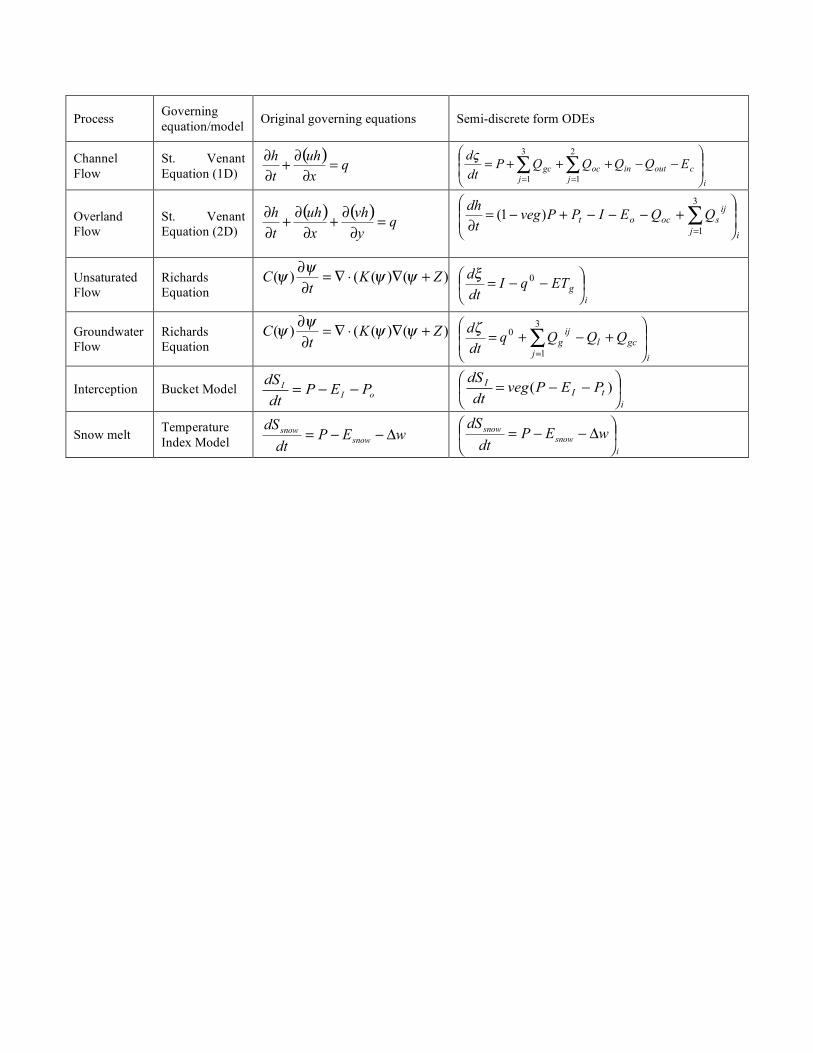
5.1. Physical process interaction PIHM is a finite volume based integrated hydrologic model. It simulates multiple physical states on discretized elements (also called model kernel) of a watershed domain. The governing equations on each model kernel are defined using an ordinary or partial differential equation (ODE or PDE). By using the Method of Lines approach, PDEs are converted to ODEs (Leveque 1994). The resulting system of ODEs is assembled and solved simultaneously using a stiff ODE solver known as CVODE (Cohen and Hindmarsh 1994). Table 2 lists the ODEs defined on a model kernel. In Table 2, P ,

tP , I ,

IE ,

oE ,

snowE , gET ,

cE are precipitation, throughflow, infiltration, and

evaporation from interception, overland flow, snow, unsaturated zone and channel respectively. ij

sQ and ij

gQ is the lateral overland flow and groundwater flow from element i to its neighbor j . ocQ and gcQ describes interaction between overland flow

and channel, and groundwater and channel respectively. 0q is internal recharge flux

between unsaturated and saturated zone. lQ is vertical leakage through an underlying confining bed. inQ and outQ are flow in and out of a channel section. w! is snow melting rate and veg is the areal vegetation fraction in a control volume.

We note that the ODEs defining rate of change of overland and ground water flow depth (Table 2) depend on the head in adjacent kernels. Similarly, channel head is dependent on lateral fluxes from upstream and downstream channel sections, and the watershed. This means that a design of the hydrologic model data structure must incorporate the topologic relationship between neighboring unit elements. In addition to these relationships, Table 3 also lists the data requirements for calculation of each physical state on every model kernel at any time. An inclusive hydrologic model data structure will account for all the data requirements at all times. The hydrologic model data structure is also influenced by the shape and adjacency of unit elements, which are in turn defined by the choice of domain decomposition (structured and unstructured) and numerical solution strategy (finite element, difference or volume) employed in modeling. 5.2. Domain Decomposition The process of discretizing the watershed into adjoining physical subdomains based on hillslopes (Band 1989), contours (Moore et al. 1988), structured or unstructured grids, is called domain decomposition. Distributed hydrologic models solve physical states on the decomposed elements of a watershed using finite difference, finite volume, and finite element methods. As mentioned previously, PIHM uses unstructured meshes to decompose the domain. The individual unit control volume elements are either prismatic (for watershed elements) or trapezoidal/cuboidal (for river elements). The basic constructs of these shapes are Nodes (vertices of the triangles) and Edges (boundaries of the triangles). The number of boundary faces through which flux exchange takes place is equal to 5 and 6 for prismatic and river elements respectively (shown in Figure 5). If a model uses structured grids to decompose the domain, then the number of faces across which flux exchange can potentially take place in 3D will be equal to 6. So the shapes of

the unit element also determine how the relationships between neighboring elements need to be represented in a hydrologic model data structure. We note that the unstructured mesh decomposition poses additional challenges in the design of hydrologic model data structure, particularly in terms of definition of topological relationships, than structured grids where the neighbors are implicitly characterized by the decomposition itself.

With the object oriented hydrologic data model in place (section 5) and the spatial relationships and parameter definitions for the hydrologic model identified (in this section), the last step in shared data model design is to re-represent the hydrologic GIS data types and the hydrologic model structure using the same feature classes thus providing an automatic connection between GIS and the hydrologic model. The next section discusses the design of this shared data model 6. Shared Data Model Design The shared data model captures the spatial structure of hydrographic features and temporal objects by identifying five classes: Node, Element, Channel, Soil and Time Series (shown in Figure 6). These classes are representational complements of the six GIS data model classes (see Figure 3) and can be obtained by applying appropriate transformations or redefinitions. The relevant geometric, spatial and topological transformations performed on GIS data types are shown in Figure 7. By generating mesh decomposition using points and lines as constraints (more details in Kumar et. al. 2008b), nodes of the triangles automatically act as the Feature Points and Edges of the triangles act as Feature Lines. Properties and attributes of boundaries of the Feature Polygon are assigned to the Element edges after converting the polygons to polyline and then to lines. Attributes of the Feature polygons and Feature Volumes are geographically registered to the triangular elements. We note that re-representation of hydrologic GIS data types are “loss-less” mappings implying that they reversible. By aggregating Element Edge, Channel or Elements based on its attribute properties, we can revert back from Shared Data model class to original GIS data objects. The operators used in re-representation of classes are shown over the lines connecting the source and result class in Figure 7. These operators are also listed as Methods (in the bottom-most compartment) in the GIS data model class diagrams (see Figure 3). Names of each of these operators are self-explanatory for their functions. We note that the dotted line in the transformation diagram indicates the intermediate results.

Figure 6 also shows the Aggregation, Uni-directional Association, Reflexive Association and Generalization relationships supported in the shared data model. An Element class represents a discretized triangular element in 2D and a prismatic element in 3D and is defined by six nodal locations listed in a clockwise direction at two levels. The prismatic element has five neighbors- three on the sides and one at the top and bottom. We note that neighbors of an element also belong to an Element class and this recursive relationship is captured by Reflexive association. The cardinality of this relationship is 1 to 5 which means that there has to be at least one neighboring element to an Element object. A maximum cardinality of 5 denotes that a 3D element can have a total of 3 lateral and 2 vertical neighbors. A Channel class is defined by the two end nodes and neighboring elements on the either side of channel. Each channel segment is also composed of an upstream and downstream channel segment which is captured by a

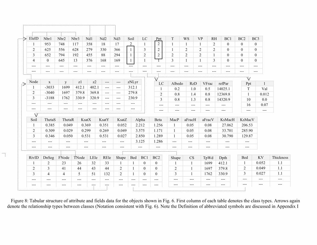
Reflexive association. We note that the multiplicity of this relationship varies from 0 to any integer value. This means that a channel segment can stand alone in the watershed with no upstream or downstream channels. A Channel is also Bi-directionally associated with an Element with a multiplicity of 1 to 2. This translates to existence of at least one neighboring triangular element to a channel segment. Bi-directionality ensures that both Element and Channel is aware of this topological relationship. These relations are fundamentally important for spatial integrity of the hydrologic modeling framework. Each Element class is also associated with Soil, Land Cover and Time Series class. This ensures clean and efficient assignment of properties to each Element. Similarly the Channel is associated to Bed Property and Shape classes. Soil Class contains several attribute fields such as Hydraulic conductivities and van-Genuchten equation soil retention parameters (van Genuchten 1980). Attributes of Land cover class are root zone depth, albedo and photosynthetically active radiation from each land cover type. We note that Precipitation, Temperature, Humidity, Incoming Solar Radiation, Ground Heat Flux, Vapor Pressure, LAI, Vegetation Fraction, Wind Velocity, Time dependent boundary conditions and the observed and simulated state variables are all instances or child objects to the Time Series Class. Name of the operators shown in Figure 5 is self-explanatory of their functions. These operators are concerned with derivation of geometric properties of triangular elements and channels or with the calculation of rate of change of state variables with time. Definitions of various functions are given in Appendix I. Figure 8 shows an example of relationships between classes using the tabular database structure corresponding to objects and its attributes. We note that due to space constraint and simplicity, the topology has been limited to lateral neighbors only and only a few instances of Time Series class (such as precipitation time series) have been tabulated in Figure 8. The shared data model design is tested in the development of a coupled GIS-hydrologic modeling system. The integrated software is an open-source, and platform independent, extensible and “tightly-coupled” integrated GIS interface to Penn State Integrated Hydrologic Model (PIHM) and is referred as PIHMgis. 7. PIHMgis PIHMgis is an integrated and extensible GIS system with data management, analysis, data modeling, unstructured mesh generation, visualization and distributed PIHM modeling capabilities. The underlying philosophy of this integrated system is a shared geo-data model between GIS and PIHM that was developed in the previous sections. The shared data model makes it possible to handle the complexity of the representation structures, data types, model simulations and analysis of results. The graphic interface component of PIHMgis has been written in Qt and C++ which supports object oriented class structures in programming. PIHMgis sits on an open source Qgis engine (www.qgis.org) and has been integrated as pluggable software. Figure 9 shows a snapshot of PIHMgis interface. The interface and the source code can be downloaded from http://www.pihm.psu.edu/pihmgis_downloads.html.

The architectural framework of the interface is shown in Figure 10. Directionality of the arrows indicates the possible flow of output from one Method to another. The flow of actions between different class objects in PIHMgis can be shown using an object

oriented UML collaboration diagram (see Figure 11). These diagrams represent both the static and the dynamic behavior of the system by representing collaboration (simple associations) between objects and mapping the sequence of messages they share between them. The rectangles in the diagram enclose the class and its instance (separated by a colon), and the links between rectangles represent the collaborations (communications) between classes. The chronological labeling of the messages between class objects describes the sequence in which actions are executed. The first communication initiated by the integrated system is from the object from where message 1.0 is released. In order to track the messages/actions that are hierarchically associated with a parent object, a nested numbering of messages is performed. Figure 11 shows that a full hydrologic modeling exercise can be carried out in PIHMgis by directly acting upon the raw data types represented in the shared data model, merely by launching a sequence of messages (commands). Starting with digital elevation model raster data, which is an instance of Grid class, Raster processing operations (RasterProcessing()::StreamDefinition; RasterProcessing():: WatershedDelineation) result in delineation of watersheds and definition of streams. On a parallel path, Very Important Points (VIPs) are extracted using other Raster Processing operations (RasterProcessing()::VIPidentification). A Vector processing tool with polyline reconditioning algorithms (VectorProcessing() :: PolylineReconditioning) simplifies and splits lines. Vector merging (VectorProcessing()::Merge) of all the available features layers is performed before they can be used as a spatial support for perform domain decomposition. Details about the need of vector processing steps and how they aid flexible domain decompositions are in Kumar et. al. (2008b). Once Domain decomposition have been performed, topology definitions and field assignment of properties is performed for each triangular element and river channel (DataModelLoader()::RiverIdentification;DataModelLoader()::AttributeAssignment;Data ModelLoader()::ForcingsAssignment). After decomposition and topology definitions, the initialization of state variable on each model kernel is carried out. Numerical solver (Solve()) formalizes all the ODEs in each model kernel in the form of )(' yfy = and then solves the system iteratively. Output results in the form of spatial and time series plots are displayed (Display::SpatialPlot();Display::TimeSeriesPlot()) in the Visualization toolkit integrated in PIHMgis. Details about all the operator functions in the PIHMgis toolkits are discussed in Bhatt et. al. (2008). The simple, compact and procedural structure of PIHMgis (see Figure 11) streamlines the process of organizing the data for model simulations. PIHMgis allows the user to perform semi-automated preliminary model simulations with minimum user input. The ease of use of the coupled system can be judged from the fact that graduate students with no prior knowledge of modeling (in an introductory groundwater modeling class) are able to perform uncalibrated simulations after two training lectures. 8. Advantages of Shared Data Model for GIS-Hydrologic Model coupling A shared data base, relationships and schemas between GIS and the hydrologic model leads to an integrated system with options to simulate model states, steer simulations and to conveniently manage, analyze and display data used and produced by the model. The

unique advantages of coupling based on a shared data model development are discussed next. 8.1. Enhanced accuracy As mentioned in Section 6, the hydrologic model grids supported by the shared data model are generated by using GIS points, polyline and polygons as constraints. The unique advantage of using GIS objects as constraints for decomposition is that the resulting model grid can be designed to follow the edges of a single property type (such as Soil or Land Cover, geology, vegetation, etc.). This limits introduction of additional data uncertainty arising from statistical averaging of multiple class themes within a model grid. Figure 12 highlights this concept, where an unstructured mesh generated using soil theme as a constraint leads to decomposition where each triangle has a single soil type. For structured grid decomposition with the same average resolution as the unstructured mesh, we observe that 41.63 % percent of the grids have mixed themes. Generating grids that do not follow edges of thematic classes (as shown in the case of structured grids) introduces uncertainty. Similarly if observation stations (point objects) are used as a constraint in decomposition, hydrologic states can be predicted exactly at the observation stations. The geo-referential integrity inherent in the shared data model minimizes any errors during comparison of observed and predicted states which creep in due to interpolation of prediction variables to the observation locations. 8.2. Storage efficiency In any watershed model, there are a limited number of parameters and forcing types (e.g. soil, land cover, precipitation etc.) which are needed to define each hydrologic property over the domain. For example in Figure 8, only two different soil and precipitation (Ppt) types are defined on all the elements. This translates to storage efficiency at two levels in a shared data model approach. First, the storage of (soil) properties as a relational object assures that these properties are accessible to both the GIS and the hydrologic model. Instead of storing all the nine soil attribute parameters (floating type numbers) as separate grids, we are able to store them as a single layer and soil type (an integer attribute of Element Class) with associative relations defined to all the nine attributes of Soil Class. The compression is even more significant in storage of forcing time series such as of Precipitation, Ppt and Temperature, T. Rather than storing the forcing grid at numerous time steps (e.g. satellite images of time series variables like temperature), the precipitation-type attribute for each element class is associated with a precipitation magnitude within a Time Series class. Significant storage efficiency is also gained due to the description of the data on constrained Delaunay triangulations. 8.3. Real-time visualization and Decision support The architectural framework of PIHMgis in Figure 10 shows that the outputs from the model simulations continually update the geodatabase of the shared data model. This means that any selected number of state variables or fluxes can be plotted at any location while the simulation proceeds. This is particularly useful in assessing whether the

simulation results are physically realistic, and gives an opportunity to make adjust the model or make management decisions in real time. A typical real time plot is shown in Figure 13. The figure illustrates all vertical fluxes at a selected element (shaded in Figure 13) for 366 days of simulation in Little Juniata Watershed. We can immediately see that recharge to groundwater is positive in winter months (from November to January ranging from 0 to 90 days), becomes negative in the summer (from July to September ranging from 240 to 330 days), and varies inversely to the total evapotranspiration. During summer, larger evapotranspiration leads to creation of negative matric potential in unsaturated zone. This translates to a negative recharge situation where water moves across the capillary fringe from the saturated zone to the unsaturated zone. Real time visualization also serves as an “early warning” system to track errors in simulation arising from wrong/bad data input or numerical “blow-up”. During the simulation the user can search for the appearance of non-physical states in real time and immediately detect problems in the solution. 8.4. Parameter steering Distributed hydrologic model calibration and sensitivity analysis of parameters requires performing multiple model simulations. Since a shared data model stores GIS data in a hydrologic model grid structure, the coupled GIS-model system provides unique flexibility in modifying parameters or forcing values in any selected portion of the watershed. For example, if it is found that during calibration the leaf area index (LAI) for a particular land cover type is resulting in underprediction of interception storage, the shared data model can efficiently query all Elements of that particular land cover type and perform the required parameter nudging. For traditional approaches with an isolated data-model and data-structures, changes in parameters (such as LAI) in a particular region would require GIS processing on the raw data and generation of new input files. In summary, a streamlined data structure and relationship definitions of a shared data model result in an efficient, integrated and automated steering of parameters 9. Conclusions This paper presents the design and details of a shared data model which can support coupling of GIS with a hydrologic model. The conceptualization and characterization of this coupling strategy can be used with other physically distributed models and can be extended to management, visualization and decision support tools (e.g. ecological models, ). The data model is rich yet flexible in terms of its extensibility and simplicity. The data model incorporates representation of wide range of data types varying from static and floating points to 3D feature line and volume objects. The object oriented strategy streamlines the design of the data model and clarifies the relationships between classes. UML class and collaboration diagrams have been developed to show the standardized static and dynamic structure of classes, their operations and activity in the larger software framework. It also provides a clear modular sequencing of operations in the coupled software. Object oriented data model design leads to seamless assimilation of the classes and their relationships directly in object oriented software development. The shared data model is successfully used to develop a prototype open-source, platform

independent coupled modeling system referred to as PIHMgis. The shared data model concept creates a process for modeling that improves data flow, model parameter development, parameter steering, efficient grid design and allows real time visualization and decision support. References ABEL, D.J. and KILBY, P.J., 1994, The systems integration problem. International

Journal of Geographical Information Systems Journal of Hydrology, 87, 61-77 ALONSO, G. and EL ABBADI, A., 1994, GOOSE: Geographic Object Oriented Support

Environment. In Proceedings of ACM/ISCA Workshop on Advances in Geographic Information Systems, pp. 38-43

BAND, L. E., 1986, Topographic partition of watersheds with digital elevation models, Water Resources Research, 23(1), 15–24.

BENNETT, D. A., 1997. A framework for the integration of geographical information systems and model base management, International Journal of Geographical Information Science, 11(4): 337–357.

BHATT, G., KUMAR, M. AND DUFFY, C.J., 2008. Bridging the gap between geohydrologic data and distributed hydrologic modeling. In Proceedings of International Congress on Environmental Modeling and Software, (accepted).

COHEN, S.D. and HINDMARSH, A.C.,1994. CVODE User Guide, LLNL Technical report UCRL-MA-118618.

FEDRA, K., 1996. Distributed Models and Embedded GIS: Strategies and Case Studies of Integration.' In: Goodchild, M.F., Steyart, L.Y., Parks, B.O., Johnston, C., Maidment, D., Crane, M. and Glendinning, S. [eds], GIS and Environmental Modeling: Progress and Research Issues, GIS World Books, Fort Collins, CO., pp.413–417

FREEZE, R.A., AND CHERRY, J.A., 1979. Groundwater, Prentice Hall: Englewood Cliffs, NJ., pp. 29.

FREEZE, R. A., and HARLAN, R. L., 1969. Blueprint for a physically-based digitally simulated, hydrologic response model, Journal of Hydrology, 9, 237– 258

GALTON, A., 2001. Space, Time, and the Representation of Geographical Reality,Topoi 20: 173-187.

GOODCHILD, M.F., 1992. Geographical information science. International Journal of Geographical Information Systems 6(1): 31-45.

HELLWEGER, F. L., and MAIDMENT, D. R., 1999. Definition and Connection of Hydrologic Elements Using Geographic Data. Journal of Hydrologic Engineering. 4(1), 10-18

HEUVELINK 1998. Error propagation in environmental modelling with GIS. Taylor and Francis, London, UK

KOPP, S. M., 1996. Linking GIS and hydrological models: where have we been, where are we going? In HydroGIS 96: Application of Geographic Information Systems in Hydrology and Water Resources (ed. by K. Kovar & H. P. Nachtenebel) 13-21. IAHS Publ. no. 235

KOLLET, S. J., and MAXWELL, R. M., 2006. Integrated surface-groundwater flow modeling: A free-surface overland flow boundary condition in a parallel groundwater flow model, Advances in Water Resources, (29)7, 945-958

KUMAR, M., BHATT, G. and DUFFY, C., 2008a. Coupling of Processes and Data in a Mesoscale Watershed, Advances and Water Resrouces.(submitted)

KUMAR, M., BHATT, G. and DUFFY, C., 2008b. Efficient domain decomposition framework for accurate representation of geodata on watershed model grid, International Journal of Geographical Information Science.(accepted)

LAHLOU, M., SHOEMAKER, L., CHOUDRY, S., ELMER, R., HU, A., MANGUERRA, H. and PARKER, A., 1998. ‘Better assessment science integrating point and nonpoint sources: BASINS 2.0 User’s Manual’,EPA-823-B-98-006, U.S. Environmental Protection Agency, Office of Water, Washington, DC, USA

LUZIO. DI, M., SRINIVASAN, R., ARNOLD, J.G., and NEITSCH, S.L., 2002. Arcview Interface for SWAT2000. User’s Guide. U.S. Depart- ment of Agriculture, Agriculture Research Service. Temple, Texas. Available at http://www.brc.tamus.edu/swatt/downloads/ doc/swatav2000.pdf Accessed on March 18, 2008

MAIDMENT, D., 1993. Developing a spatially distributed unit hydrograph by using GIS. In Proceedings of Applications of GIS in hydrology and water resources (edited by Kovar, K. and Nachtenebel, H.), Vienna. IAHS publ. no. 211. 181-192.

MAIDMENT, D., 2002. Arc Hydro: GIS for Water Resources. Redlands, CA, ESRI Press MARTIN, R., 2002. Agile Software Development, Principles, Patterns, and Practices.

Prentice Hall. MARTIN, P.H., LEBOEUF, E.J., DOBBINS, J.P., DANIEL, E.B., and ABKOWITZ, M.D., 2004.

Development of a GIS-Based Spill Management Information System. Journal of Hazardous Materials, B112:239-252.

MCKINNEY, D.C., and CAI, X.M., 2002. Linking GIS and water resources management models: an object-oriented method. Environmental Modeling & Software, 17, 413-425.

MILNE, P., MILTON, S., and SMITH, J., 1993. Geographical Object-oriented Databases: a Case Study. International Journal of Geographical Information Systems, 7:39-56.

MOORE I. D. , O’LOUGHLIN, E. M., and BURCH. A., 1988. Contour-based topographic model for hydrological and ecological applications, Earth Surface Processes Landforms,13,305-320.

NATIONAL RESEARCH COUNCIL ,1999. New Strategies for America’s Watersheds. Washington DC, National Academy Press

NELSON, E.J., 1997. WMS v5.0 Reference Manual, Environmental Modeling Research Laboratory, Brigham Young University, Provo, Utah, 462 pp.

NYERGES, T. L.1993. Understanding the scope of GIS: It’s relation to environmental modeling. In M. F. Goodchild, B. O. Parks, & L. T. Steyaert, eds. Environmental Modeling with GIS. Oxford University Press.

PANICONI, C., KLEINFELDT, S., DECKMYN, J., and GIACOMELLI, A., 1999. Integrating GIS and data visualization tools for distributed hydrologic modelling. Transactions in GIS. 3(2), 97-118.

QU, Y., and DUFFY, C. J., 2008, A semidiscrete finite volume formulation for multiprocess watershed simulation, Water Resources Research, 43

RAPER, J.F. and LIVINGSTONE, D.,1995. Development of a Geomorphological Spatial Model Using Object-oriented Design. International Journal of Geographical Information Systems, 9(4):359-383.

SMITH, P. N., and MAIDMENT, D. R., 1995. Hydrologic Data Development System, CRWR Online Report 95-1, Center for Research in Water Resource, The University of Texas at Austin, Austin, TX.

VAN GENUCHTEN, 1980. A closed-form equation for predicting hydraulic conductivity of unsaturated soils, Soil Sciences Society of America Journal, 44:892-898

WATKINS, D. W., MCKINNEY, D. C., MAIDMENT, D. R., and LIN, M., 1996. Use of geographic information systems in ground-water flow modeling. Journal of Water Resources Planning and Management, ASCE, 122(2), 88–96

WILSON, J.P., INSKEEP, W. P., WRAITH, J. M., and SNYDER, R. D., 1996. GIS-based solute transport modeling applications: Scale effects of soil and climate data input. Journal of Environmental Quality 25: 445-53

WILSON, J. P., 1999. Current and future trends in the development of integrated methodologies for assessing non-point source pollutants. In D L Corwin, K Loague, and T W Ellsworth (eds) Assessment of Non-Point Source Pollution in the Vadose Zone. Washington DC, American Geophysical Union: 343-61

WRIGHT, D.J., BLONGEWICZ, M.J., HALPIN, P.N. and BREMAN, J., 2007. Arc Marine: GIS for a Blue Planet, Redlands, CA: ESRI Press, 202 pp

Appendix I List of Symbols aFracH: aerial fraction of macropore in horizontal soil section aFracV: aerial fraction of macropore in vertical soil section Albedo: albedo (reflective fraction) of a land cover type Alpha: van-Genuchten scaling parameter Beta: van-Genuchten relaxation parameter BC1: Boundary condition on edge 1 of a traingle BotFP: Bottom Feature Polygon CS: River cross-section type DnSeg: Downstream River segment ID FNode: Upstream Node vertex of a channel segment TNode: Downstream Node vertex of a channel segment Ksat_X: Horizontal saturated conductivity in X-direction Ksat_Y: Horizontal saturated conductivity in Y-direction Ksat_Z: Vertical saturated conductivity in Z-direction KsatMac: Saturated Macropore conductivity KV: Vertical Conductivity of river bed LC: Land Cover LeftL_X: Lower Left x-coordinate location LeftL_Y: Lower Left y-coordinate location Nbr1: Neighboring element of a triangular element Nd1: Vertex node of a triangular element NumCol: Number of Columns in Grids NumFl: Number of Feature Lines in a Polygon NumPts: Number of points in a Feature Line NumRow: Number of Rows in Grids

t: Time Point_TopFP: Pivot point in Top polygon boundary of Feature Volume Point_BotFP: Pivot point in Bottom polygon boundary of Feature Volume Ppt.: Precipitation Time series refPar: reference incoming solar flux for photosynthetically active canopy RH: Relative Humidity Time series RzD: Rootzone Depth Theta_S: Maximum porosity Theta_R: Residual porosity TopFP: Top Feature Polygon Val_(NumRow*NumCol): Field value at grid location (NumRow, NumCol) vFrac: Vegetation Fraction VP: Vapor Pressure Time Series WS: Wind Speed Time Series ySurf: Overland Flow Depth yRiv: River stage ySubSurf: Moisture head List of Functions areaChannel(): Function to calculate cross-section area of the channel element areaElement(): Function to calculate surficial area of the prismatic element effK(): Effective conductivity of the subsurface frictionSlope(): Function to calculate friction slope Interpoaltion(): Function to interpolate value of a time series at any time using the parsimonious information in Time Series data structure yDotRiv(): Function to calculate rate of change of river stage yDotSurf(): Function to calculate rate of change of overland flow depth yDotSubSurf(): Function to calculate rate of change of moisture head Figures

Figure 1: Conceptual classification of existing GIS data types relevant to hydrologic modeling Figure 2: (a) Three compartment structure of Class icons. Options listed inside curly or large brackets are optional. (b) Cardinality/Multiplicity notation of relationships in a Class Diagram Figure 3: GIS data model class diagram design for hydrologic data in UML 2.0. Note the type and cardinality of relationships between various classes (details in Section 3.1). The operators in the bottom compartment for each individual class are used in transformation of GIS data model into a shared data model structure that is valid on hydrologic model grids. Figure 4: Feature object designs for a) Point b) Polyline c) Polygon and d) Volume. Note the implicitness of the “sequence of constructs” in Feature Polygon and Feature Volume design. (c) shows that edge polylines of the the polygon are always listed in clockwise direction. Similarly, definition of a 3D feature necessities pivot point and boundary polygons in a particular sequence. Note that the identification of one point from both top and bottom polygon in design of Feature Volume is done in order to pivot the connection sequence of the nodes of the two polygons which results in a 3D feature Figure 5: Prismatic and River Kernel in PIHM. The number of interaction fluxes between neighbors is equal to 5 for the prismatic kernel and 6 for the river kernel. Figure 6: Shared data model class diagram design for GIS-Hydrologic Model coupling in UML 2.0. Note the type and cardinality of relationships between various classes (details in section 3.3.3). Figure 7: Class Re-Representation diagram showing the transformation of a GIS based data model classes into Classes identified in Shared Data Model design. The arrows originate from each individual GIS data model class and end in the corresponding complement shared data model class. Operators/Functions that perform this transformation are shown along the arrows. Dotted arrows represent intermediate transformation operations. Figure 8: Tabular structure of attribute and fields data for the objects shown in Fig. 6. First column of each table denotes the class types. Arrows again denote the relationship types between classes (Notation consistent with Fig. 6). Note the Definition of abbreviated symbols are discussed in Appendix I Figure 9: A snapshot of the derived unstructured decomposition of Little Juniata Watershed in a GIS-Hydrologic Model coupled PIHMgis Interface. Note the toolbar on the top left which performs Raster Processing, Vector Processing, Domain Decomposition, Data Model Loader, PIHM simulation and Analysis operations.

Figure 10: Architectural framework of PIHMgis. Directionality of the arrows indicates the possible flow of output from one module to another Figure 11: Collaboration diagram showing the dynamic activity sequence of classes in PIHMgis. The rectangles denote the class instance, the directionality of arrows denotes the flow of action and nested numbering keep track of the sequence of operations in a global framework. An example of a hierarchical nesting sequence is 1 1.1 1.1.1. Shaded boxes denote the independent initiation (trigger) of operations. Figure 12: Top left unstructured mesh decomposition (UnSrG) is generated based on thematic class (soil type) boundary as constraint. Top right structured mesh (SrG) decomposition has same spatial resolution as the grid on left. Colored grid in the background of both the decompositions is a soil type map. The zoomed-in image shows that SrG (in light grey) have multiple soil classes within them. UnSrG edges (in red or dark grey (in black and white)) overlap soil class edges thus resulting in a “one soil class assignment” to each triangle Figure 13: Simulataneous plots of vertical fluxes (et0 ! Evaporation from canopy, et1! Transpiration, et2 ! Evaporation from ground, Recharge! Recharge to ground water) at the shaded element after 366 days of simulation in Little Juniata Watershed.

Tables Table 1: Characteristics of different levels of integration between a GIS and a hydrologic model Table 2: Differential equations of hydrologic processes on a model kernel. Table 3: Data requirements for calculation of physical states on a model kernel at any simulation time

Figure 1: Conceptual classification of existing GIS data types relevant to hydrologic modeling

3D Line

Examples: Meandering river with dynamic bank, Estuary Bdd.

2D Line Floating

Static Static

Floating

Static

Floating

Regular

Irregular

Hydrologic GIS Data Types

Examples: TINs, Sensor Network Configurations

Tessellations

Examples: Remote Sensed Image,

Elevation, Land Cover, Soil

2D

Examples: Geology

3D

Line

Examples: River, Subshed Bdd., Fault

Lines

2D Line

Examples: Pumping Wells, Underground Pipe Networks

Point

Examples: Stage (Weir), Wind Speed

(Anemometer), Precipitation (Gauge),

Flux Tower, Water Table (Well)

Isotropic

Examples: Saturated Hydraulic Conductivity, Manning’s Coefficient

Anisotropic

Examples: Infrequent Measurement Samples (Field Campaigns) for Water Table, Soil Moisture

Polygon

Examples: Soil, Geology,

Watershed Bdd.,

Examples: Lake, Flooded Area

Examples: Precipitation, Temperature, Wind Speed

Time Series

Object Field

(a) (b) Figure 2: (a) Three compartment structure of Class icons. Options listed inside curly or large brackets are optional. (b) Cardinality/Multiplicity notation of relationships in a Class Diagram

Class

Attribute Name [multiplicity]: Type = Initial value {Property String}

Operation (Attribute: Type): Return Type {Property String}

Multiplicity Notation

Explanation

1 One Instance

0..1 0 or 1 instance

0..* or * 0 or more instances

0..n 0 to n instances

Figure 3: GIS data model class diagram design for hydrologic data in UML 2.0. Note the type and cardinality of relationships between various classes (details in Section 3.1). The operators in the bottom compartment for each individual class are used in transformation of GIS data model into a shared data model structure that is valid on hydrologic model grids.

X! : Double Y! : Double Z! : Double

Anisotropic Point

Floating Point

t: Double

Feature Polygon (FP)

ID: Int NumFl: Int Line_1: FL Line_2: FL …………… Line_NumFL: FL Value: Double/String

VectorProcessing( Polygon:FP): FL

Feature Point (FPt) ID: Int X: Double Y: Double Z: Double Value: Double/String VectorProcessing(Point:FPt):NODE

Feature Line (FL) ID: Int NumPts: Int Point_1: FPt Point_2: FPt ………….. Point_NumPts: FPt Value: Double/String VectorProcessing( Line:FL): EDGE

Feature Volume (FP)

ID: Int Point_TopFP: Fpt Point_BotFP: Fpt TopFP: FP BotFP: FP Value: Double/String DataModelLoader(Volume:FP)

Grid ID: Int LeftL_X: Double LeftL_Y: Double NumRow: Int NumCol: Int Val_1: Double Val_2: Double …………….. …………….. Val_(NumRow*NumCol): Double DataModelLoader(Grid)

2..NumPts

2

3..NumFL

Feature Classes

Time Series ID: Int Length: Double T_1: Double Val_1: Double T_2: Double Val_2: Double …………….. …………….. T_Length: Double Val_Length: Double

DataModelLoader(Time Series)

Relationships Association Generalization Aggregation

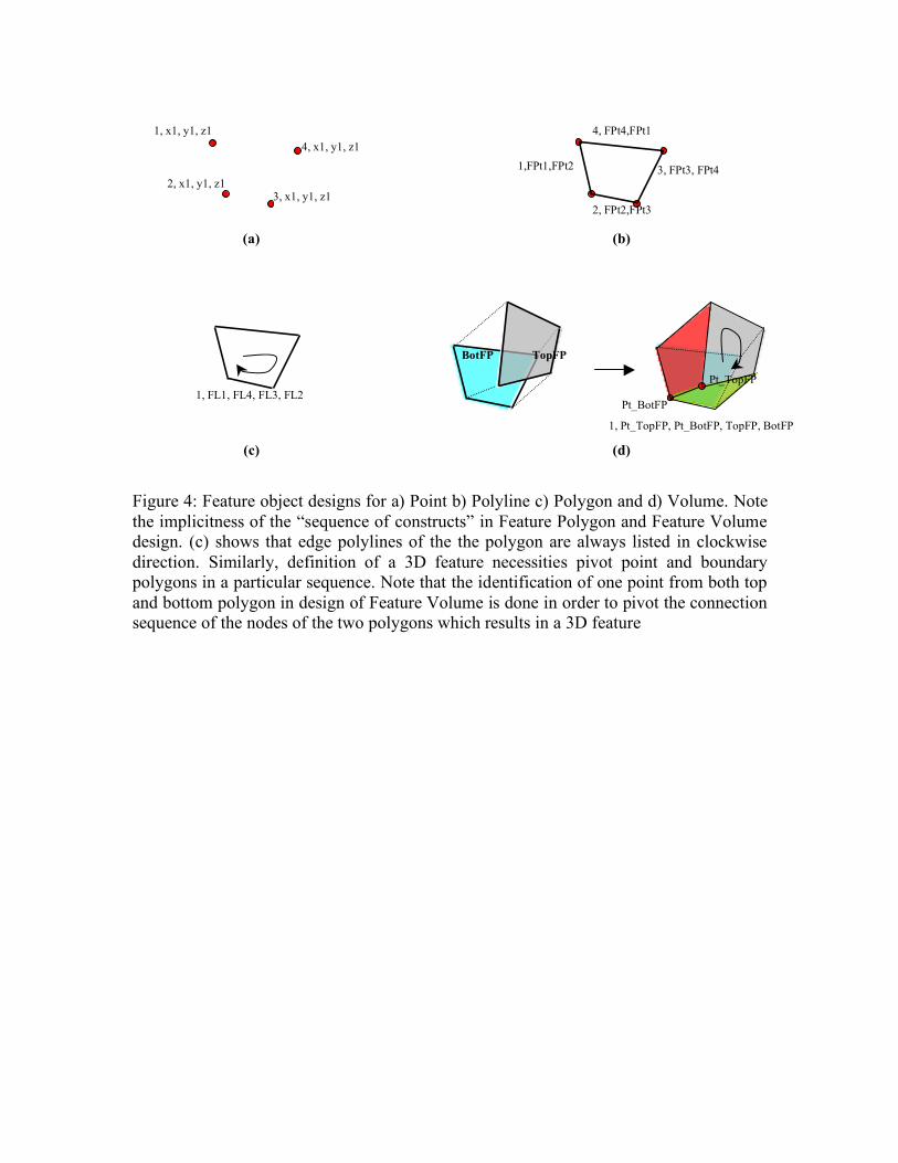
Figure 4: Feature object designs for a) Point b) Polyline c) Polygon and d) Volume. Note the implicitness of the “sequence of constructs” in Feature Polygon and Feature Volume design. (c) shows that edge polylines of the the polygon are always listed in clockwise direction. Similarly, definition of a 3D feature necessities pivot point and boundary polygons in a particular sequence. Note that the identification of one point from both top and bottom polygon in design of Feature Volume is done in order to pivot the connection sequence of the nodes of the two polygons which results in a 3D feature

1, x1, y1, z1

2, x1, y1, z1 3, x1, y1, z1

4, x1, y1, z1 1,FPt1,FPt2 3, FPt3, FPt4

2, FPt2,FPt3

4, FPt4,FPt1

TopFP BotFP

Pt_TopFP

Pt_BotFP 1, FL1, FL4, FL3, FL2

(a) (b)

(c) (d)

1, Pt_TopFP, Pt_BotFP, TopFP, BotFP

Figure 5: Prismatic and River Kernel in PIHM. The number of interaction fluxes between neighbors is equal to 5 for the prismatic kernel and 6 for the river kernel.

Unsaturated Zone

Saturated Zone

River Zone

qo

Qg Qg

Qin

Prismatic Kernel River Kernel

Qg

Qout

Qgc

Qoc

Prismatic elements

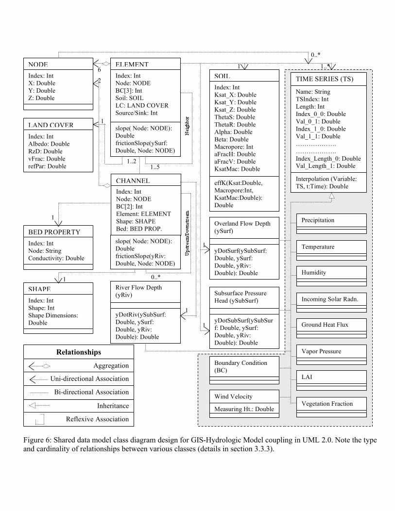
Figure 6: Shared data model class diagram design for GIS-Hydrologic Model coupling in UML 2.0. Note the type and cardinality of relationships between various classes (details in section 3.3.3).

Relationships

Aggregation

Uni-directional Association

Inheritance

Reflexive Association

6 Index: Int Node: NODE BC[3]: Int Soil: SOIL LC: LAND COVER Source/Sink: Int

ELEMENT

slope( Node: NODE): Double frictionSlope(ySurf: Double, Node: NODE)

1..5 1..2

Precipitation

Temperature

Humidity

Incoming Solar Radn.

Ground Heat Flux

Vapor Pressure

Measuring Ht.: Double

Wind Velocity

LAI

Vegetation Fraction

Name: String TSIndex: Int Length: Int Index_0_0: Double Val_0_1: Double Index_1_0: Double Val_1_1: Double ………………. ………………. Index_Length_0: Double Val_Length_1: Double

TIME SERIES (TS)

Interpolation (Variable: TS, t:Time): Double

Boundary Condition (BC)

Subsurface Pressure Head (ySubSurf)

yDotSubSurf(ySubSurf: Double, ySurf: Double, yRiv: Double): Double

Overland Flow Depth (ySurf)

yDotSurf(ySubSurf: Double, ySurf: Double, yRiv: Double): Double

River Flow Depth (yRiv)

yDotRiv(ySubSurf: Double, ySurf: Double, yRiv: Double): Double

Index: Int Ksat_X: Double Ksat_Y: Double Ksat_Z: Double ThetaS: Double ThetaR: Double Alpha: Double Beta: Double Macropore: Int aFracH: Double aFracV: Double KsatMac: Double Roughness: Double

SOIL

effK(Ksat:Double, Macropore:Int, KsatMac:Double): Double

Index: Int Shape: Int Shape Dimensions: Double

SHAPE

Index: Int X: Double Y: Double Z: Double

NODE

2

Index: Int Node: String Conductivity: Double

BED PROPERTY

Index: Int Node: NODE BC[2]: Int Element: ELEMENT Shape: SHAPE Bed: BED PROP.

CHANNEL

slope( Node: NODE): Double frictionSlope(yRiv: Double, Node: NODE)

0..*

1

1

1

1

1

1 1..*

0..*

Bi-directional Association

Index: Int Albedo: Double RzD: Double vFrac: Double refPar: Double

LAND COVER 1

Figure 7: Class Re-Representation diagram showing the transformation of a GIS based data model classes into Classes identified in Shared Data Model design. The arrows originate from each individual GIS data model class and end in the corresponding complement shared data model class. Operators/Functions that perform this transformation are shown along the arrows. Dotted arrows represent intermediate transformation operations.

Data Model Loader: Attributes Assignment

Feature Polygon (FP)

Feature Point (FPt)

Feature Line (FL)

Feature Volume (FP)

Grid

Time Series

Node

Element Edge

Channel

Time Series

Vector Processing: Polygon to Line

Vector Processing: Split Line At Nodes

Vector Processing: Constraint Assignment

Element Data Model Loader: Topology Definition

Vector Processing: Constraint Assignment

Data Model Loader: Forcings Assignment

GIS data model Classes

Shared data model Classes

EleID Nbr1 Nbr2 Nbr3 Nd1 Nd2 Nd3 Soil LC Ppt T WS VP RH BC1 BC2 BC3 1 953 748 117 358 18 17 2 1 2 1 1 1 2 0 0 0 2 625 556 628 279 330 366 1 3 2 1 2 2 2 0 0 0 3 652 794 192 455 88 294 1 2 2 2 2 2 1 0 0 0 4 0 645 13 376 168 169 1 1 1 3 1 1 3 0 0 0

--- --- --- --- --- --- --- --- --- --- --- --- --- --- --- --- --- --- --- --- --- --- --- --- --- --- --- --- --- --- --- --- --- ---

Figure 8: Tabular structure of attribute and fields data for the objects shown in Fig. 6. First column of each table denotes the class types. Arrows again denote the relationship types between classes (Notation consistent with Fig. 6). Note the Definition of abbreviated symbols are discussed in Appendix I

Node x y z1 z2 --- --- zNLyr 1 -3033 1699 412.1 402.1 --- --- 312.1 2 -3040 1697 379.8 369.8 --- --- 279.8 3 -3188 1762 330.9 320.9 --- --- 230.9 --- --- --- --- --- --- --- --- --- --- --- --- --- --- --- ---

LC Albedo RzD VFrac refPar 1 0.2 1.0 0.5 14025.1 2 0.8 1.4 0.8 12369.8 3 0.8 1.3 0.8 14320.9 --- --- --- --- --- --- --- --- --- ---

Ppt 1 T Val 1 0.012 10 0.0 16 0.07 --- ---

Soil ThetaS ThetaR KsatX KsatY KsatZ Alpha Beta MacP aFracH aFracV KsMacH KsMacV 1 0.385 0.049 0.369 0.351 0.052 2.212 1.256 1 0.05 0.08 27.062 206.53 2 0.309 0.029 0.299 0.269 0.049 3.575 1.171 1 0.05 0.08 33.701 285.90 3 0.346 0.050 0.531 0.531 0.027 2.850 1.289 1 0.05 0.08 30.790 129.87

--- --- --- --- --- --- 3.125 1.286 --- --- --- --- --- --- --- --- --- --- --- --- --- --- --- --- --- ---

Shape CS TpWd Dpth 1 1 1699 412.1 2 1 1697 379.8 3 1 1762 330.9 --- --- --- --- --- --- --- ---

RivID DnSeg FNode TNode LEle REle Shape Bed BC1 BC2 1 2 23 26 32 33 1 1 0 0 2 3 41 44 43 44 2 1 0 0 3 4 4 5 51 132 2 1 0 0 --- --- --- --- --- --- --- --- --- --- --- --- --- --- --- --- --- --- --- ---

Bed KV Thickness 1 0.052 1.1 2 0.049 1.1 3 0.027 1.1 --- --- --- --- --- ---

Figure 9: A snapshot of the derived unstructured decomposition of Little Juniata Watershed in a GIS-Hydrologic Model coupled PIHMgis Interface. Note the toolbar on the top left which performs Raster Processing, Vector Processing, Domain Decomposition, Data Model Loader, PIHM simulation and Analysis operations.

Figure 10: Architectural framework of PIHMgis. Directionality of the arrows indicates the possible flow of output from one module to another.

Geodatabase (Schema, Data, Relationships)

Field, Feature Objects, Non-Spatial Data

User Interface

Vector Processing

Raster Processing

Data Model Loader

Parameterization

Data Management Kernel Definition

Numerical Solver

PIHM Spatial

Temporal

Data Analysis

Spatio-Temporal

Uncertainty

Static: Conformed, constrained Delaunay &

nested triangulation

Dynamic: Adaptive triangulations

Domain Decomposition

(Grid-Shp/ Dbf) Read, (Grid-Shp/ Dbf) Write

Data Accessor

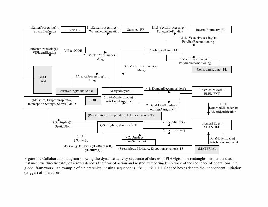
Figure 11: Collaboration diagram showing the dynamic activity sequence of classes in PIHMgis. The rectangles denote the class instance, the directionality of arrows denotes the flow of action and nested numbering keep track of the sequence of operations in a global framework. An example of a hierarchical nesting sequence is 1 1.1 1.1.1. Shaded boxes denote the independent initiation (trigger) of operations.

7: DataModelLoader():: ForcingsAssignment

2.1:VectorProcessing():: Merge

7.1: yInitialize()

4:VectorProcessing():: Merge

7.1.1: { Solve() ;

ConstrainingPoint: NODE

DEM: Grid

1:RasterProcessing():: StreamDefiniton River: FL Subshed: FP

VIPs: NODE

1.1:RasterProcessing():: WatershedDelineation

2:RasterProcessing()::VIPidentification

InternalBoundary: FL

3.1:VectorProcessing():: Merge

1.1.1.1VectorProcessing():: PolylineReconditioning

MergedLayer: FL

ConstrainingLine : FL

1.1.1:VectorProcessing():: PolygonToPolyline

ConditionedLine : FL

UnstructureMesh : ELEMENT

4.1: DomainDecomposition()

Element Edge : CHANNEL

(Precipitation, Temperature, LAI, Radiation): TS

:SOIL

:MATERIAL

3:VectorProcessing():: PolylineReconditioning

5: DataModelLoader():: AttributeAssignment

4.1.1: DataModelLoader():: RiverIdentification

6: DataModelLoader():: AttributeAssignment

(ySurf, yRiv, ySubSurf): TS 6.1: yInitialize()

[yDotSurf(), yDotSubSurf(), yDotRiv()] }

yDot = (Streamflow, Moisture, Evapotranspiration): TS

(Moisture, Evapotranspiratio, Interception Storage, Snow): GRID

7.2: Display(): TimeSeriesPlot

7.3: Display(): SpatialPlot

Figure 12: Top left unstructured mesh decomposition (UnSrG) is generated based on thematic class (soil type) boundary as constraint. Top right structured mesh (SrG) decomposition has same spatial resolution as the grid on left. Colored grid in the background of both the decompositions is a soil type map. The zoomed-in image shows that SrG (in light grey) have multiple soil classes within them. UnSrG edges (in red or dark grey (in black and white)) overlap soil class edges thus resulting in a “one soil class assignment” to each triangle

Figure 13: Simulataneous plots of vertical fluxes (et0 ! Evaporation from canopy, et1! Transpiration, et2 ! Evaporation from ground, Recharge! Recharge to ground water) at the shaded element after 366 days of simulation in Little Juniata Watershed.

et0

0

0.0006

0.0012

0.0018

0.0024

0.003

0 30 60 90 120 150 180 210 240 270 300 330 360

et0

et2

0

0.0006

0.0012

0.0018

0.0024

0.003

0 30 60 90 120 150 180 210 240 270 300 330 360

et2

et1

0

0.0006

0.0012

0.0018

0.0024

0.003

0 30 60 90 120 150 180 210 240 270 300 330 360

et1

Recharge

-0.001

-0.0004

0.0002

0.0008

0 30 60 90 120 150 180 210 240 270 300 330 360

Recharge

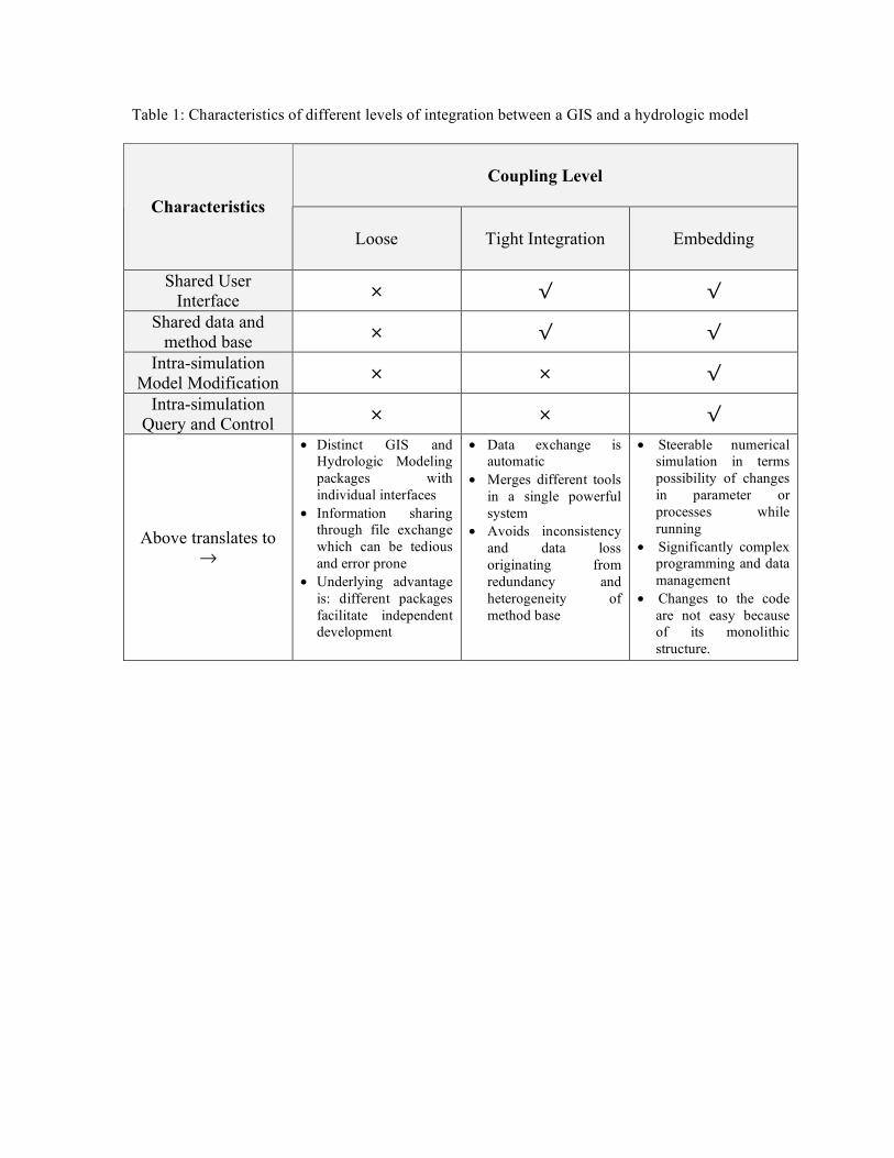
Table 1: Characteristics of different levels of integration between a GIS and a hydrologic model

Coupling Level

Characteristics

Loose Tight Integration Embedding

Shared User Interface × √ √

Shared data and method base × √ √

Intra-simulation Model Modification × × √

Intra-simulation Query and Control × × √

Above translates to !

• Distinct GIS and Hydrologic Modeling packages with individual interfaces

• Information sharing through file exchange which can be tedious and error prone

• Underlying advantage is: different packages facilitate independent development

• Data exchange is automatic

• Merges different tools in a single powerful system

• Avoids inconsistency and data loss originating from redundancy and heterogeneity of method base

• Steerable numerical simulation in terms possibility of changes in parameter or processes while running

• Significantly complex programming and data management

• Changes to the code are not easy because of its monolithic structure.

Process Governing equation/model Original governing equations Semi-discrete form ODEs

Channel Flow

St. Venant Equation (1D)

( )q

x

uh

t

h=

!

!+

!

! i

coutin

j

oc

j

gc EQQQQPdt

d

!!"

#$$%

&''+++= ((

==

2

1

3

1

)

Overland Flow

St. Venant Equation (2D)

( ) ( )q

y

vh

x

uh

t

h=

!

!+

!

!+

!

! ij

ijsocot QQEIPPveg

t

dh

!!"

#$$%

&+'''+'=

( )=

3

1

)1(

Unsaturated Flow

Richards Equation

)()(()( ZKt

C +!"!=#

#$$

$$

i

gETqIdt

d!"#

$%& ''=

0(

Groundwater Flow

Richards Equation

)()(()( ZKt

C +!"!=#

#$$

$$

i

gcl

j

ijg QQQq

dt

d

!!"

#$$%

&+'+= (

=

3

1

0)

Interception Bucket Model oI

IPEP

dt

dS!!=

i

tII PEPvegdt

dS!"

#$%

& ''= )(

Snow melt Temperature Index Model wEP

dt

dS

snow

snow!""=

i

snow

snowwEP

dt

dS!"

#$%

& '((=

Process Data Support

Channel Flow

Head in adjacent triangular elements, Head in river segment downstream and upstream, Initial head value at the start of simulation, Precipitation, Evaporation, Manning’s coefficient, Coefficient of discharge for weir flow across river bank, Elevation of end nodes of river segment, Leakage coefficient, Subsurface flow head in adjacent triangles, boundary conditions Note: Head Overland Flow (unless specified otherwise)

Overland Flow

Head in neighboring elements, Head in river segment (if river is neighbor to the cell), Initial head value, Net Precipitation, Evapotraspiration, Elevation of nodes of triangular element, boundary conditions Note: Head Overland Flow

Unsaturated Flow

Capillary flow, Initial head value, subsurface flow head, Infiltration, hydraulic conductivity, evapotranspiration, root uptake, soil porosity, Van genuchten soil parameters, boundary conditions Note: Head Unsaturated Flow

Groundwater Flow

Head in adjacent triangles, Initial Head value, capillary flow, hydraulic conductivity of the elements and its neighbors, Bedrock depth, soil porosity, Van genuchten soil parameters, boundary conditions Note: Head Groundwater Flow

Interception Interception storage capacity, Precipitation, LAI, Evapotranspiration, initial interception

Snow melt

Initial snow depth, initial snow density, initial snow surface layer temperature, initial average snow cover temperature, average snow liquid water content, net solar radiation, incoming thermal radiation, air temperature, vapor pressure, wind speed, soil temperature, precipitation

Infiltration Overland flow head, unsaturated soil moisture, hydraulic conductivity, porosity, macropore, precipitation rate, maximum infiltration capacity

Evapotranspiration Wind speed, Humidity, Net radiation, soil heat flux, vapor pressure deficit, mean air density, Interception storage capacity, LAI, soil saturation, atmospheric resistance, stomatal resistance, vegetation fraction, unsaturated zone saturation