HAL Id: hal-02541808https://hal.archives-ouvertes.fr/hal-02541808

Submitted on 14 Apr 2020

HAL is a multi-disciplinary open accessarchive for the deposit and dissemination of sci-entific research documents, whether they are pub-lished or not. The documents may come fromteaching and research institutions in France orabroad, or from public or private research centers.

L’archive ouverte pluridisciplinaire HAL, estdestinée au dépôt et à la diffusion de documentsscientifiques de niveau recherche, publiés ou non,émanant des établissements d’enseignement et derecherche français ou étrangers, des laboratoirespublics ou privés.

Distributed under a Creative Commons Attribution| 4.0 International License

An open-source Abaqus implementation of thephase-field method to study the effect of plasticity onthe instantaneous fracture toughness in dynamic crack

propagationGergely Molnar, Anthony Gravouil, Rian Seghir, Julien Réthoré

To cite this version:Gergely Molnar, Anthony Gravouil, Rian Seghir, Julien Réthoré. An open-source Abaqus implementa-tion of the phase-field method to study the effect of plasticity on the instantaneous fracture toughnessin dynamic crack propagation. Computer Methods in Applied Mechanics and Engineering, Elsevier,2020, 10.1016/j.cma.2020.113004. hal-02541808

An open-source Abaqus implementation of the phase-field method to

study the effect of plasticity on the instantaneous fracture toughness in

dynamic crack propagation.

Gergely Molnara,∗, Anthony Gravouila, Rian Seghirb, Julien Rethoreb

aUniv Lyon, INSA-Lyon, CNRS UMR5259, LaMCoS, F-69621, FrancebEC Nantes, CNRS UMR6183, GeM, F-44300, France

Abstract

Brittle and ductile dynamic fracture in solids is a complex mechanical phenomenon which attractedmuch attention from both engineers and scientists due to its technological interests. Modeling cracksin dynamic cases based on a discontinuous description is difficult because it needs additional criteriafor branching and widening. Due to the very short time scales and the spatial complexity of thedynamic problem, its experimental analysis is still very difficult. Therefore, researchers still have torely on numerical simulations to find a deeper explanation for many observed phenomena. This studyis set out to investigate the effect of plasticity on dynamic fracture propagation. On the other hand,the diffuse phase-field formulation makes it possible to initiate, propagate, arrest or even branchcracks while satisfying the basic principles of thermodynamics. An implicit, staggered elastoplasticversion of the phase-field approach was implemented in the commercial finite element code Abaqusthrough the UEL option. By means of simple examples we show that localized ductile deformationsfirst increase both resistance and toughness. Then, after a maximum value, the resistance starts todecrease with a significant increment in energy dissipation. By favoring shear deformation over tensilefailure the fracture pattern changes. First the branching disappears, then the crack propagation anglechanges and becomes a shear band. Finally, we observed the increment of the instantaneous dynamicstress intensity factor during the acceleration stage of the crack without introducing a rate dependentcritical fracture energy. We explained this phenomenon with the increasing roughness of the fracturesurface.

Keywords: Dynamic fracture, Ductile fracture, Phase-field, Abaqus UEL, Dynamic stress intensityfactor

1. Introduction

Fracture is the most feared failure mode in solids and structures. Both brittle and ductile crackpropagation can lead to life threatening and devastating financial consequences. Therefore, a predic-tive description of the phenomenon is of great importance to both scientists and engineers equally.One of the earliest successful descriptions were proposed by Griffith [1]. The criterion was based onan energy balance equation. Griffith postulated that if the release rate of the strain energy is higherthan a critical value, the preexisting crack propagates. The theory became very popular because thecritical energy release rate was found to be a material constant for measuring the fracture toughness

∗Corresponding authorEmail address: gergely.molnar@insa-lyon.fr (Gergely Molnar)

Preprint submitted to Computer Methods in Applied Mechanics and Engineering April 14, 2020

of brittle materials. The original description did not consider the actual motion and the dynamics ofthese events. Since then, considerable experimental [2, 3, 4, 5] and theoretical studies [6, 7, 8, 9] werededicated to understanding the underlying physics and mechanics. However, due to the complexityof the problem, dynamic fracture is still an active area of research.

Beyond a few theoretical cases, practical engineering examples are usually too complex to besolved using analytical techniques. Therefore, numerical methods play a key role in fracture analysis.To model cracks both discrete and continuum methods can be utilized. Molecular dynamics [10,11] provide a valuable insight into the physics of crack initiation, however neither the length northe time scales is sufficient for practical applications. Discrete element simulations [12] solve thescaling problem, however their use is mostly limited to highly inhomogeneous materials (e.g. granularmater or rocks). Nevertheless, even if discrete techniques propose some advantages, the continuumdescription is the most commonly used approach. The finite element method was shown to be ableto model dynamic fracture with the help of various enrichments. The cohesive zones method [13, 14]is based on the separation of predefined surfaces assuming a finite process zone located at the frontof the fracture. The so-called strong discontinuity approach [15] adds a finite displacement step atthe crack front. In more recent years the eXtended finite element method [16] was successfully usedto follow dynamic crack propagation in elastic [17] and ductile [18] cases. Generally, branching wasidentified as an instability and the loss of hyperbolicity [19, 20] of the acoustic matrix. The abovementioned methods represent fracture as discrete discontinuities. Therefore, initiation or branchingof cracks were proven to be a complicated task and often needed a special criteria.

Nonlocal damage models [21, 22, 23, 24] provide an alternative description. The thick level setapproach determines the crack path based on the damage evolution at the crack tip, and the dis-continuity is introduced explicitly. While in other smeared models, such as the phase-field approach,discontinuities are not used directly. Instead, a smooth transition characterizes the effect of the crack.A single damage variable connects the fully damaged region to the intact material. The applicationof nonlocal damage models to Griffith’s theory is based on the variational formulation of Francfortand Marigo [25, 26] and the phase-field implementation of Bourdin [27].

The reversibility of the damage field [28] was first enforced by prohibiting the crack from healing.This formulation leads to a minimization principle with inequality constraints, which is challengingto implement in most finite element methods [29]. Departing from the original idea, Miehe et al. [30]proposed a prevalent approach by introducing a new field variable, the history of the maxima of theelastic (undamaged) energy.

Two main numerical techniques are used in practice to solve the mechanical problem and find thephase-field topology: the monolithic (fully coupled) [31, 32, 33, 34, 35, 36] and the staggered (weaklycoupled) [27, 30, 37, 38, 39] scheme. Monolithic algorithms usually converge when the initial estimateis close to the equilibrium solution. However, in the case of e.g., unstable crack initiation, they failto find a definitive solution. This problem is due to the convexity of the global energy and the jumpsin the solution [40]. Various modifications [40, 41, 34] were proposed to circumvent these issues.

The staggered scheme is based on the alternating minimization algorithm of Bourdin et al. [27].Two well-posed, convex problems are solved independently. While the damage and the elastic strainenergy is passed between the two equations only at the beginning of the time step. This iterativeprocess was proven to be very robust, even in unstable cases [38]. The only disadvantage of themethod that it requires a relatively small time step [39]. In this work, a common variant is used[30, 42, 43], when the iteration around the two decoupled problems is not performed. In quasi-staticcases, for unstable propagation, this could violate the energy conservation of the system. Therefore,we controlled the time step automatically to detect unstable propagation and reduce the change in theexternal loading. Since the first introduction of the method, numerous open-source implementations

2

were proposed [32, 44, 39, 33]. For a detailed overview on the history the reader is referred to thework of Bourdin [45].

Since the method was originally introduced, it became surprisingly popular in the fracture sciencecommunity. Several implementations were proposed to follow dynamic [46, 47, 48, 49, 50, 51, 52] andductile [53, 54, 55, 56, 57, 58, 59, 60] fracture. Surprisingly, formulations concentrating on the effectof plasticity on the dynamic crack propagation is still scarce. Only two implementations [61, 62]exist with details on the development of the theory and some examples. Despite the benefits, theuse of phase-fields is still limited in practice because none of the commonly available finite elementsoftware provide it as a built-in option. Recently Liu et al. [63] published a dynamic phase-field modelusing Abaqus, however their subroutine is still reserved for private use. A smart implementation wasproposed recently by Azinpour et al. [64], who used the built-in thermal module of the software andused the temperature field as damage. Furthermore, hydrogen induced cracking [65] and a coupledcohesive zone model [35] was implemented in Abaqus using either UMATs or UELs. Both authorsprovide an open-source version of their codes.

Crack propagates in an unstable or dynamic manner if the energy release rate increases withcrack growth. Therefore, the surplus of released energy can be transformed into kinetic energy. Thedifference between the fracture toughness and the additional energy release determines how muchenergy becomes available as kinetic energy and consequently governs the speed at which the crackpropagates. Finally, if the energy release exceeds twice the critical value, the crack branches. It iscommonly assumed that very close to the crack tip a so-called process zone forms. In this region thematerial starts dissipating energy (e.g. by plasticity) to regularize the stress singularity. As a result,the macroscopic fracture resistance is higher for more ductile materials. These properties are knownto depend upon strain rate. For example at higher deformation rates, the yield strength is higheras well. It was postulated theoretically [2] and observed experimentally [66], that the instantaneousfracture toughness (stress intensity factor in this case) of most materials (even in brittle ones) increaseswhen the crack accelerates. The magnitude of this increment is of course different for brittle andductile materials. In general, strain rate sensitive materials, such as ferritic steels will show largervariations in the measured stress intensity factor than rate insensitive ones such as high strengthsteel of aluminum alloys [67]. The uniqueness of the relation between crack velocity and macroscopicfracture toughness is questioned by several authors [68, 66]. However, there is still no theoreticalstudy which explains if this phenomenon is a geometrical effect, or if there should be a unique law todescribe the rate dependent fracture surface energy for each material. It would be crucial to clarifythis question, as most engineering guidelines [67] and numerical methods (e.g. XFEM [69]) use thelaw of Kanninen [2] to decide if the crack can propagate and at which speed it runs.

Motivated by the popularity [60] of our recent open-source Abaqus phase-field implementationfor static cases [70], we wish to extend the subroutine to dynamic, ductile and coupled cases in both2D and 3D. The new implementation contains all options and proposes switch variables to the userto decide which option should be used. We implemented the popular staggered time integrationscheme [30] for rectangular and triangular (tetrahedral in 3D) elements. Presently, a von Mises [71]type plastic criterion is implemented, which is gradually degraded with damage. This allows us todirectly take the plastic energy into account when calculating the fracture topology. Optionally, apenalty function is included if only an ultimate strain value is available for the user.

Through simple examples the validity of the implementation is proved by comparison to analyticsolutions and results from literature. Finally, with the help of the newly formulated element westudy the impact of plasticity on the fragmentation patterns, the crack velocity and the macroscopicfracture toughness in dynamic crack propagation.

As a summary, we propose a robust and versatile open-source subroutine for practical engineers

3

as well as research scientists in a widely available commercial finite element code Abaqus. Theimplementation can be used to study both brittle and ductile static and dynamic fracture.

The paper is structured as follows: Section 2 presents the theory of the elasto-plastic dynamicphase-field formulation. Section 3 asses the effect of the yield parameters in the quasi-static case.While section 4 shows 2D and 3D dynamic crack topologies, and section 5 presents the instantaneousfracture toughness obtained using the Abaqus implementation. Finally, Section 6 concludes the paper.

2. Methods

2.1. Phase-field approximation of the fracture surface

The principal idea of the phase-field formulation for fracture is the introduction of an internallength scale (lc). Thus, this method diffuses the sharp crack into the volume of the elastoplastic solidas illustrated in Fig. 1.

By introducing damage variable (d), a smooth transition is created from undamaged (d = 0) tobroken material (d = 1). Miehe [31] introduced the crack surface density:

γ (d,∇d) =1

2lcd2 +

lc2|∇d|2. (1)

This approximation uses the spatial gradient of the damage field to describe the crack topology.The volume integral of eq. (2) on the whole body gives the theoretical fracture surface:

Γ =

∫Ω

γ (d,∇d) dΩ. (2)

Our previous work [70] provides further details about the theory of the basic phase-field formula-tions.

2.2. Energy functional

The energy functional of the elastoplastic dynamic problem involves the following Lagrangianfunction:

L = D (u)− Π (u, d) , (3)

where D (u) is the kinetic energy:

D (u) =1

2

∫Ω

uT uρdΩ, (4)

and Π (u, d) is the potential energy:

Π (u, d) = E (u, d) + P (u, d) +W (d) . (5)

In eq. (4) u contains components of the velocity vector, while ρ is the mass density. The potentialenergy is constructed from three components: the (i) elastic strain energy (E), (ii) plastic strainenergy (P ) and the (iii) fracture energy (W ). All components depend on either the phase-field (d)or the displacement field (u). The following sections are dedicated to discuss the details of theorybehind each energy component.

4

2.2.1. Elastic strain energy

Classically the elastic strain energy density is composed of a tensile (ψ+0 ) and a compression

components (ψ−0 ):

E (u, d) =

∫Ω

ψel (u, d) dΩ, (6)

ψel (u, d) = g (d)ψ+0

(εel (u)

)+ ψ−0

(εel (u)

). (7)

The decomposition of the elastic strain energy [24] is meant to account for degradation upontension, while the material remains intact upon compression. g (d) is the degradation function:

g (d) = (1− d)2 + k, (8)

where k is a small 10−8 number responsible for numerical stability.Depending on the implementation, the definition of the positive and negative energy parts can

vary. In our case for brittle materials, we consider:

ψel (ε, d) = µ3∑i=1

[〈εi〉2− + g (d) 〈εi〉2+

]+λ

2

[g (d) 〈tr (ε)〉2+ + 〈tr (ε)〉2−

]. (9)

While for the ductile case, we assume that the material is damaged equally under the shear incompression and extension [37, 72]:

ψel (ε, d) = g (d)

[µ

3∑i=1

ε2i +

λ

2〈tr (ε)〉2+

]+λ

2〈tr (ε)〉2− . (10)

The overall strain field is divided into elastic (εel) and plastic parts (εpl):

ε = εel + εpl. (11)

While assuming small deformations, where the strains are defined by the symmetric part of thedeformation gradient:

ε = ∇Su. (12)

Details considering the elastic stress and stiffness calculation can be found in Appendix A.We note that in the ductile case, if the shear is applied under severe hydrostatic compression,

volumetric locking can spoil the final results [73]. As in this paper, we use fracture cases mostly inextension we did not have to deal with the phenomenon published recently for purely shear drivencracks. However, if the end-user wants to apply the program for compression fracture cases, thisshould be tackled appropriately [74, 75, 56].

2.2.2. Plastic strain energy

The plastic energy can be expressed as:

P (u, d) =

∫Ω

g (d)ψpl0

(εpl (u)

)dΩ =

∫Ω

∫t

(εpl : σ

)dtdΩ, (13)

5

where σ is the damage degraded Cauchy stress tensor (see eq. (A.3)). Present implementationsupports the von Mises [71] yield criterion:

f (σ) = σeq − g (d)[σlim +Hεpleq

], (14)

with σeq as the von Mises stress (calculated equally from the degraded Cauchy stress). As thereis no permanent volume change, the ductile part of the energy history can be expressed as a functionof the yield stress and the energy equivalent plastic shear strain [76]:

ψpl0

(εpleq (u)

)= εpleq (u)

[σlim +

1

2Hεpleq (u)

]+

1

2Iε⟨εpleq − εcreq

⟩2, (15)

where σlim is the von Mises yield strength, H is the hardening modulus and εpleq is the energyequivalent plastic shear strain. The last term in eq. (15) with the positive part function1 is a penaltycomponent which assures that the material breaks at a given critical strain. Iε is chosen accordingto the considerations discussed in Appendix C.

It can be noticed that with the evolution of the damage the yield strength of the material graduallybecomes zero, allowing plasticity to initiate and guide fracture. Additionally, the UEL option allowsthe user to implement any desired yield criterion. Current formulation allows us to treat the plasticproblem as a classical von Mises type model, for which details can be found in various textbooks [77,76].

If the plastic option is active, plastic deformation under axial ompression and tension contributesthe same way to damage. Thus, the switch variables in the energy decomposition are αi=1,2,3 = 1independently of the sign of the principal strains. Details can be found in Appendix A. An anisotropicHill yield criterion [78] could be an alternative treatment for this problem. Furthermore, we considerthe effect of stress triaxiality [62] on the yield function essential to reproduce the experimentallyobserved crack nucleation in plastic materials. However, the implementation of such approach isbeyond the scope of present paper.

2.2.3. Fracture energy

The main idea of the phase-field approach is that the discontinuity is smeared and treated asa continuous field between damaged and intact materials. Therefore, the fracture energy can beexpressed from eq. (2) as a function of the damage variable (d) itself:

W 0 (d) =

∫Γ

gcdΓ ≈∫Ω

gcγ (d,∇d) dΩ =

∫Ω

gc2lc

[d2 + l2c |∇d|

2] dΩ, (16)

where γ is the fracture energy density, gc is the surface energy needed to create a unit fracturesurface and lc is the length scale parameter which measures the scale of the damage diffusion.

Interestingly, a slightly different fracture energy density was proposed by Fremond [79] whichprovides an elastic threshold:

W (d) =

∫Ω

ψc[2d+ l2c |∇d|

2] dΩ. (17)

Note that compared to eq. (16), in eq. (17) d enters the formulation by a linear term.

1〈•〉 = (•+ |•|)/2

6

After certain algebraic manipulations Miehe [55] achieved a very similar form to their originalformulation:

W (d) =

∫Ω

t (d) + w0 (d) dΩ, (18)

where t (d) will act as a threshold energy in the staggered formulation (see later):

t (d) = ψc − g (d)ψc. (19)

ψc = gc/2lc was chosen, as a result w0 became identical to eq. (16):

w0 (d) = 2lcψcγ (d,∇d) =gc2lc

[d2 + l2c |∇d|

2] (20)

This equation remains fixed. However, to switch between the classic solution [30] and the elasticthreshold the user can set ψc to zero in t (d). Thus omitting the initial change in the energy history.

2.3. Staggered time-integration algorithm

There is an ongoing discussion whether the monolithic or the staggered scheme should be usedin practice. In the case of unstable crack propagation, the monolithic solution [31] tends to becomenumerically unstable as the algorithm needs to find the fully formed crack path in only one iteration,which is of-course impossible. There are various techniques, such as viscous regularization [40], pathfollowing algorithms [41], or even globalization [34], which can improve the solution. However, noneof them are suitable for the code implemented in Abaqus. Therefore, present the paper focuses onthe staggered scheme with the history variable proposed by Miehe et al. [30]. This method solvedthe topological problem and provided incredible robustness to the technique.

The basic idea is that the displacement and the phase-field problems are coupled only weakly.In each iteration they are independent and interact only through a so-called history field. In Fig. 1the schematic illustration of the staggered algorithm is shown. The sharp crack is regularized bythe phase-field which is calculated based on the energy history. Then, the damage field is used torecalculate the displacement distribution.

The energy of the displacement problem is formulated as follows:

Πu = D (u)− E (u, d)− P (u, d) + Πext (21)

where Πext is the external work done by the body (γ) and boundary (t) forces:

Πext =

∫Ω

γ · udV −∫∂Ω

t · udA. (22)

By taking the variation of eq. (21), the corresponding strong form can be obtained:

δΠu = 0 ∀δu→ ∇σ − γ = ρu in Ωσ · n = t on ΓNu = u on ΓD.

(23)

This is then solved for u, assuming d is constant.Similarly, the Lagrangian equation of the phase-field problem is written as:

Πd =

∫Ω

[gcγ (d,∇d) + g (d)H]dΩ, (24)

7

Figure 1: Illustration of the staggered scheme for solving the phase-field problem in elastoplastic solids. lc controls theapproximate width of the damaged zone.

where the potential energy from the displacement problem is replaced by the history field2:

H0 = 0

Hn+1 = max

ψ+

0 + ψpl0 − ψcHn

.

(25)

Furthermore, this formulation enforces the irreversibility of the damage (d ≥ 0). Thus, thehistory field satisfies the Karush–Kuhn–Tucker conditions. Finally, the corresponding strong formcan be expressed as:

δΠd = 0 ∀δd→ gclc

(d− l2c∆d) = 2 (1− d)H in Ω

∇d · n = 0 on Γd. (26)

Due to the limitations of the UEL option of Abaqus, the two problems are solved at the sametime independently based on the variables obtained in the previous iteration. In Fig. 2 a flowchartshows the basic iteration process.

The staggered scheme is implemented so that the two elements are connected through only thecommon block. For dynamic cases Abaqus uses the Hilber-Hughes-Taylor (HHT) [80] method toobtain equilibrium. HHT solves the linearized equilibrium problem applying the following Newton-Raphson iteration: [

Sun 00 (1 + α) Kd

n

] [un+∆t

dn+∆t

]= −

[run

αrdn−1 − (1 + α) rdn

], (27)

where run and rdn are the residues, Kun and Kd

n are the elementary stiffness matrices of the dis-placement and phase-field problems at time tn. un+∆t and dn+∆t are the new nodal solutions at

2If the energy decomposition is not used, both tension (ψ+0 ) and compression (ψ−

0 ) energy densities contribute toH.

8

Figure 2: Flowchart of the staggered solution used to implement the coupled displacement phase-field solution inAbaqus.

tn + ∆t.For details about the static calculations, the reader is referred to our previous paper [70].In the dynamic case the displacement residue contains an inertial component as well (f inen ) and

can be expressed as:

run = (1 + α) f intn − αf int

n−1 + f inen − f extn , (28)

where f extn is the external and f intn is the internal force vector. Parameter α is a damping coefficient,

which by default is set to α = −0.05.The tangent matrix of the displacement problem contains both materials stiffness (Ku

n) and mass(M) matrices:

Sun = Mdu

du+ (1 + α) Ku

n, (29)

where the acceleration derivative is assumed to take the following form with β = (1− α)2/4:

du

du=

1

β∆t2. (30)

All the corresponding residue vectors and stiffness matrices can be found either in Appendix B orin our previous paper [70].

3. Effect of yield parameters

In this section, through simple static examples the effect of each yield parameter will be explained.Our aim is to demonstrate, how plasticity can dominate the fracture process and sometimes alter thecrack path.

3.1. Yield strength

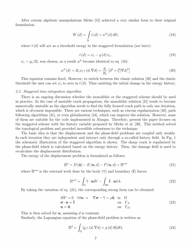
A single 2D plane strain element is the simplest case, where the phase-field model can be un-derstood. A rectangular plate with dimensions of 1 mm × 1 mm is subjected to simple shear bymoving its top side in the x direction while constraining its bottom. The shear modulus was set toµ = 80.77 GPa with H = 5 GPa, gc = 5 · 10−3 J/mm2, lc = 0.1 mm and Iε = 0. Fig. 3 shows thecorresponding von Mises stress as a function of the applied strain for different yield strength values.

9

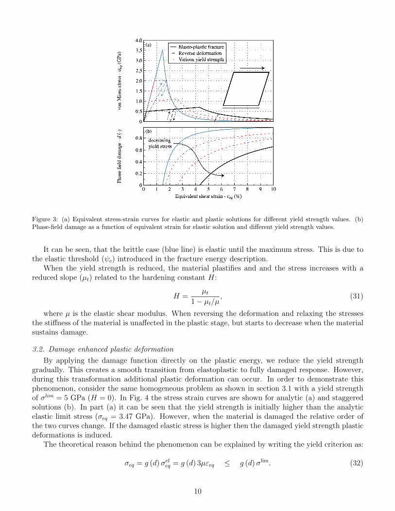
Figure 3: (a) Equivalent stress-strain curves for elastic and plastic solutions for different yield strength values. (b)Phase-field damage as a function of equivalent strain for elastic solution and different yield strength values.

It can be seen, that the brittle case (blue line) is elastic until the maximum stress. This is due tothe elastic threshold (ψc) introduced in the fracture energy description.

When the yield strength is reduced, the material plastifies and and the stress increases with areduced slope (µt) related to the hardening constant H:

H =µt

1− µt/µ, (31)

where µ is the elastic shear modulus. When reversing the deformation and relaxing the stressesthe stiffness of the material is unaffected in the plastic stage, but starts to decrease when the materialsustains damage.

3.2. Damage enhanced plastic deformation

By applying the damage function directly on the plastic energy, we reduce the yield strengthgradually. This creates a smooth transition from elastoplastic to fully damaged response. However,during this transformation additional plastic deformation can occur. In order to demonstrate thisphenomenon, consider the same homogeneous problem as shown in section 3.1 with a yield strengthof σlim = 5 GPa (H = 0). In Fig. 4 the stress strain curves are shown for analytic (a) and staggeredsolutions (b). In part (a) it can be seen that the yield strength is initially higher than the analyticelastic limit stress (σeq = 3.47 GPa). However, when the material is damaged the relative order ofthe two curves change. If the damaged elastic stress is higher then the damaged yield strength plasticdeformations is induced.

The theoretical reason behind the phenomenon can be explained by writing the yield criterion as:

σeq = g (d)σeleq = g (d) 3µεeq ≤ g (d)σlim. (32)

10

Figure 4: Shear stress and yield strength as a function of applied deformation: (a) analytic solution, (b) staggeredsolution with relatively large strain increments.

This equation can be simplified by g (d), and it can be shown that plastic deformation becomesindependent of damage. Thus, when the elastic (undamaged) stress crosses the initial yield strength,plasticity takes over. The macroscopic response will be affected slightly due to this phenomenonas the degradation function is quadratic and the absolute difference is negligible compared to themaximum stress value. Nevertheless, caution is advised when analyzing plastic strain fields aroundthe crack path.

The increased plastic deformation originates from comparing a local (stress based plasticity) to anonlocal quantity (damage). To improve the description Miehe [81] used a gradient plasticity model,where the equivalent plastic multiplier was treated as an independent degree of freedom. However,in our implementation, to remain general and to allow the end users to implement any desired yieldcriterion, we kept the local description of the plastic material model.

Fig. 4(b) shows the staggered solution of the same problem. The strain steps are intentionallyenlarged to demonstrate the issue at hand. When they are decreased, the stress result convergesto the analytic one. Due to the solution scheme explained in Fig. 2, the damage is delayed by 2time steps. This way, the elastic stress can sometimes overcome the theoretical damage threshold.Evidently, to avoid this problem it is recommended to perform a convergence analysis on the timestep size, however there are cases when the reduction of the macroscopic time step will not affect thelocal strain increments. One well known example is the departure of an unstable crack propagation.

3.3. Complex static problem

To demonstrate the effect of the yield strength on the static fracture topology the classic singleedge notched specimen is used. In Fig. 5a the geometry of the model is depicted. The bottom sideis constrained in both x and y directions, while the top is extended in the y direction maintainingux = 0. The Young’s modulus was set to 210 GPa with a Poisson’s ratio of 0.3. No hardeningwas applied, and the penalty term was also omitted (Iε = 0). The fracture properties were set to

11

Figure 5: Single edge notched specimen: (a) geometry; (b) horizontal fracture for high yield strength; (c) shear bandfor low yield strength cases; (d) reaction force as a function of the top side displacement.

gc = 2.7 · 10−3 J/mm2 and lc = 6 · 10−3 mm. The right hand side of the model, where the fracture isexpected, was meshed in an unstructured manner with hFEM = 3 · 10−3 mm size elements.

To control the time step an automatic integration scheme is used. The increment of the historyfield was limited to dH = ψc. However, in case of an unstable crack initiation the increment of Hbecomes independent of the time step. When this phenomenon is detected, the step is limited to aminimum of ∆uminy = 10−12 mm. This way, the unstable crack propagation is identified precisely.However, we note that this problem is not present in dynamic cases.

Fig. 5(b) and (c) show the fracture pattern as a function of the yield strength. It can be seen,that if σlim is sufficiently low, the fracture favors a tilted angle and the propagation is led by plasticshear deformation. This kind of shear localization is called shear banding [82].

In Fig. 5(d) the reaction force is shown as a function of the top side’s displacement. It can beseen, that for high yield strength cases (brittle, σlim = 3, 4 GPa) the crack initiates and propagatesin an unstable manner. While for lower σlim values it remains stable and a plateau is present. Theseresults show how the addition of plasticity increases the fracture toughness of the configuration. In-terestingly, by adding a small amount of plastic yield (σlim = 4 GPa) not only the toughness but theresistance of the material becomes higher. However, by further reducing σlim the resistance decreasessignificantly with the increment of the energy dissipation.

4. Fracture pattern

To determine the effect of plasticity on the dynamic crack propagation patterns, as well as tovalidate our implementation, two well-known benchmark examples are used. First, a 2D plate isloaded with an instantaneous traction stress on the top and bottom boundaries. Secondly, a 3Dslab is pre-extended statically (without damage), then the dynamic fracture is followed using thephase-field method.

4.1. 2D dynamic branching

The geometry of the 2D test is shown in Fig. 6(a). Two different finite element tessellations weretested: (i) an irregular one shown in Fig. 6(b) with ∼92 000 elements, where the right hand side of themodel is densified randomly with hFEM = 0.125 mm size rectangular elements; and (ii) a structured

12

Figure 6: Rectangular plate subjected to uniform unidirectional dynamic traction: (a) Geometry with dimensions inmm; (b) random finite element mesh with a refined zone (hFEM = 0.125 mm) in the expected propagation zone.

one, where all sides are partitioned equally with the same hFEM , creating a 256 000 element model.The Young’s modulus is set to 32 GPa with a Poisson’s ratio of 0.2. The density is 2450 kg/m2, withfracture properties gc = 3 J/m2 and lc = 0.5 mm. Neither hardening (H = 0), nor strain penalty(Iε = 0) is applied. The time step was set to ∆t = 10−8 s.

In the following sections the obtained results are discussed as a function of the yield strength: (i)fracture topology, (ii) crack velocity and finally in section 5 (iii) the instantaneous stress intensityfactor .

First, to verify our implementation, we compared our fracture pattern to ones obtained in Ref. [48]. When the elastic threshold was suppressed (ψc = 0) the fracture patterns were in agreement.However, when the elastic threshold option was used, the crack started to propagate later as well asthe branching occurred after a longer crack path. This is due to the fact that the material becamemore resistant with ψc. Fig. 7(a) and (b) also shows that in the elastic case the crack is confined,while in Borden’s work it can diffuse more into the material.

Our next comparison will focus on the difference between structured and unstructured mesh. It canbe seen in Fig. 7(b) and (c) that the mesh has a significant effect on the branching. Unfortunately, indynamic calculation the wave propagation is significantly affected by the uniformity of the mesh [83].Thus, when an instability occurs (like a branching) it will be influenced by the symmetry of thevelocity field. Note, that this phenomenon was already observed in static calculations [70].

Finally, the effect of the yield strength can be seen in Fig. 7(c-e). By reducing the yield strengththe branching disappears as the local kinetic energy is being consumed by plasticity. Then, if σlim isdecreased further, similarly to the static case, the crack starts to propagate in the direction of shearrather than the tensile mode.

Fig. 7(f) shows the equivalent plastic shear strain along the shear band in the case of σlim = 2 GPa.It can be seen that the plastic deformation has localized around the damaged zone to a band-like

13

shape. However, as highlighted in section 3.2, the actual value of the plastic strain should be treatedwith caution because of the enhancing effect of the phase-field formulation. The leaking shown in part(e) is present in almost all dynamic phase-field models if the simulation is conducted long enough, asthe kinetic energy is not entirely dissipated when the crack reaches the boundaries. Therefore, theremaining waves concentrate usually at the damaged outer region.

For quantitative comparison, the crack tip velocity is shown in Fig. 8. The position of the cracktip was calculated as the largest extension of the phase-field where its value is larger then d > 0.9 inthe lower half of the model (y < 0). An agreement was found between our work and Borden’s [48]. Itcan be seen, that adding an elastic threshold the fracture initiates and branches later, but reaches thesame maximum velocity. This velocity limit is in good correspondence with the theoretical limit [84]related to the Rayleigh wave speed (vR).

It can be observed that the velocity at the initiation of the crack slows down by reducing the plasticyield strength which is mostly due to the loss of rigidity around the crack tip. For σlim = 2 GPa,when a shear localization occurs, the maximum velocity cannot really be defined as damage developsat the same time along the shear band.

4.2. Effect of plane stress state

All techniques which are used to distinguish between tensile and compression energies are basedon the decomposition of a 3D stiffness tensor. While by omitting the third directional strain this canbe simplified for plane strain cases, in the plane stress state εz is not zero. Therefore, in elasticity thecomponents of the stiffness matrix is modified to reproduce a σz = 0 state.

Unfortunately, the energy decomposition routines used for phase-field simulations are not suitedfor plane stress cases. Therefore, to analyze the effects of σz being zero, a simple 3D trick is applied.The same geometry is created as shown in Fig. 6, however the plate is extruded in the z directionand the thickness is meshed with one element. To achieve the plane stress state all the nodes wereleft free in the perpendicular (z) direction.

In Fig. 9 the crack tip velocity is shown for different yield strength as a function of time. Thesame phenomenon is visible as in plane strain cases, the crack tip slows down as the yield strengthdecreases. For the brittle material we did not observe a significant difference between the planestrain and plane stress cases. Unfortunately, neither the temporal nor the spatial resolution of thesimulation is high enough to capture the difference caused by the 2 % decrease in the dilatationalwave speed.

On the other hand, the fracture pattern shows a significant difference for the ductile cases. In theplane stress case the straight fracture (as seen in Fig. 7(d)) never appears. After the branching, theshear band forms between the main branch and the side of the specimen. Finally, at σlim = 1.5 MPathe fracture pattern is identical to Fig. 7(e).

4.3. Pre-stressed 3D slab

In the previous two cases, when an instantaneous traction is applied on the two opposite surfaces,the shock wave traveled in a relatively homogeneous manner, therefore the 3D effect of the cracktip [67] was not visible.

Recently, Henry & Adda-Bedia [50] and Bleyer & Molinari [85] showed that initiation, propagationand branching of a crack is a truly 3D phenomenon. In this paper our aim is to partially reproducetheir results in order to validate our implementation, however due to the demanding computationalcost we concentrate on simple examples where the asymmetric energy degradation has a significanteffect.

14

Figure 7: Fracture pattern as a function of the yield strength and mesh uniformity. Comparison of part (a) should bemade with the work of Borden et al. [48].

15

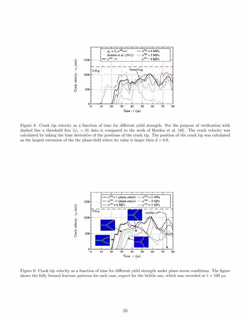
Figure 8: Crack tip velocity as a function of time for different yield strength. For the purpose of verification withdashed line a threshold free (ψc = 0) data is compared to the work of Borden et al. [48]. The crack velocity wascalculated by taking the time derivative of the positions of the crack tip. The position of the crack tip was calculatedas the largest extension of the the phase-field where its value is larger then d > 0.9.

Figure 9: Crack tip velocity as a function of time for different yield strength under plane stress conditions. The figureshows the fully formed fracture patterns for each case, expect for the brittle one, which was recorded at t = 100 µs.

16

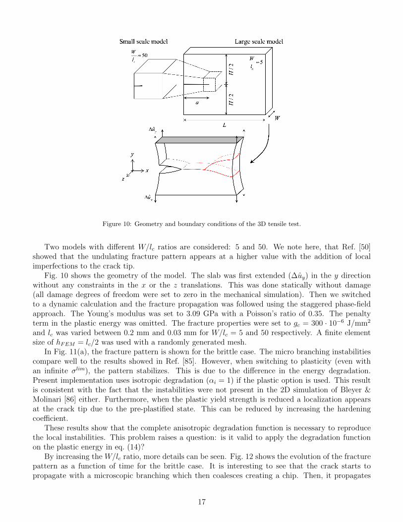
Figure 10: Geometry and boundary conditions of the 3D tensile test.

Two models with different W/lc ratios are considered: 5 and 50. We note here, that Ref. [50]showed that the undulating fracture pattern appears at a higher value with the addition of localimperfections to the crack tip.

Fig. 10 shows the geometry of the model. The slab was first extended (∆uy) in the y directionwithout any constraints in the x or the z translations. This was done statically without damage(all damage degrees of freedom were set to zero in the mechanical simulation). Then we switchedto a dynamic calculation and the fracture propagation was followed using the staggered phase-fieldapproach. The Young’s modulus was set to 3.09 GPa with a Poisson’s ratio of 0.35. The penaltyterm in the plastic energy was omitted. The fracture properties were set to gc = 300 · 10−6 J/mm2

and lc was varied between 0.2 mm and 0.03 mm for W/lc = 5 and 50 respectively. A finite elementsize of hFEM = lc/2 was used with a randomly generated mesh.

In Fig. 11(a), the fracture pattern is shown for the brittle case. The micro branching instabilitiescompare well to the results showed in Ref. [85]. However, when switching to plasticity (even withan infinite σlim), the pattern stabilizes. This is due to the difference in the energy degradation.Present implementation uses isotropic degradation (αi = 1) if the plastic option is used. This resultis consistent with the fact that the instabilities were not present in the 2D simulation of Bleyer &Molinari [86] either. Furthermore, when the plastic yield strength is reduced a localization appearsat the crack tip due to the pre-plastified state. This can be reduced by increasing the hardeningcoefficient.

These results show that the complete anisotropic degradation function is necessary to reproducethe local instabilities. This problem raises a question: is it valid to apply the degradation functionon the plastic energy in eq. (14)?

By increasing the W/lc ratio, more details can be seen. Fig. 12 shows the evolution of the fracturepattern as a function of time for the brittle case. It is interesting to see that the crack starts topropagate with a microscopic branching which then coalesces creating a chip. Then, it propagates

17

Figure 11: Fracture pattern for the 3D large scale test with different formulations.

Figure 12: Fracture pattern for the 3D small scale test.

straight until it branches macroscopically. This phenomenon is indeed due to the effect of the localelastic contraction at the crack tip [67].

After the analysis of the fracture patterns, the instantaneous stress intensity factor is calculatedto investigate the issue of the velocity toughening mechanism of the crack propagation.

5. Instantaneous fracture toughness

The correlation between dynamic (instantaneous) fracture toughness (KID) and crack tip velocity(vcr) is a well documented phenomenon [66]. It was shown that most materials exhibit an incrementin KID when the crack accelerates. Kanninen [2] proposed the following a generalized description:

KID (vcr) =KIC

1−(vcrvl

)m , (33)

where KIC is the static fracture toughness in mode I opening, vl is the maximum propagationvelocity and m is a material constant. It was shown that not only the material but also the geometryof the experiment has a significant effect on the observed results [66]. Therefore, the relationship canhardly be considered a unique material property. This is a significant problem, because when usingother simulation techniques (e.g. XFEM [69]) the kinetics of the crack is determined by the aboverelationship which is assumed to be a material property.

18

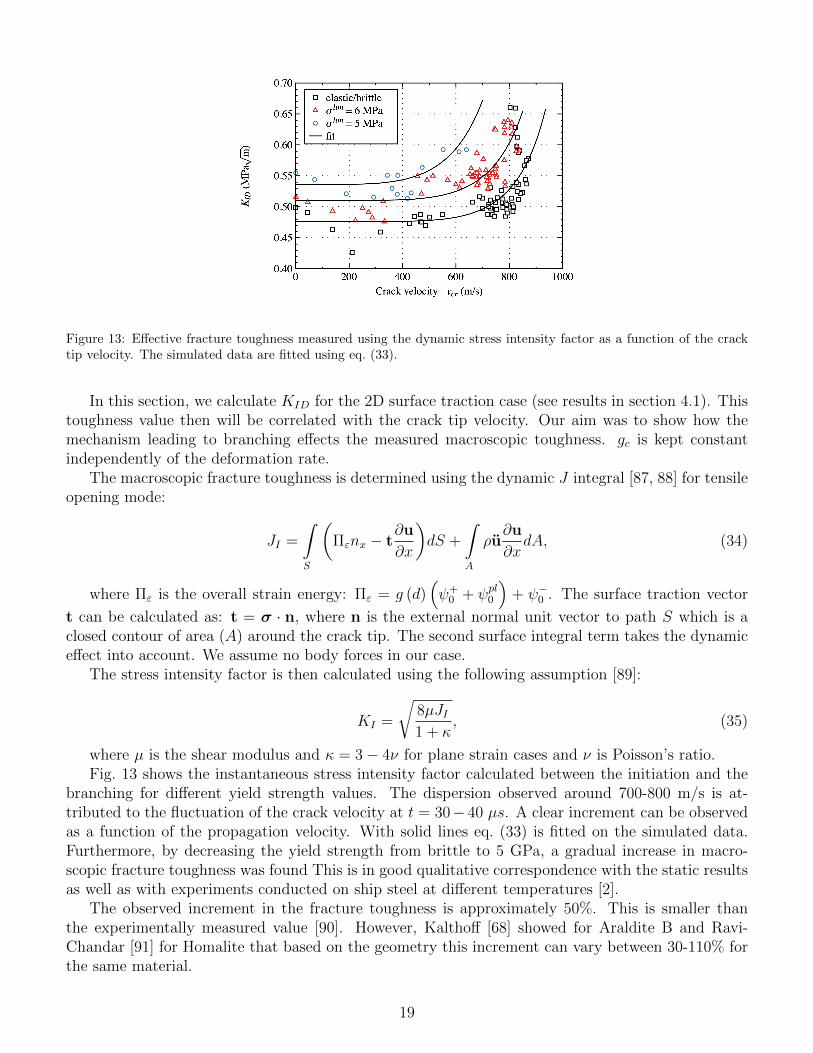
Figure 13: Effective fracture toughness measured using the dynamic stress intensity factor as a function of the cracktip velocity. The simulated data are fitted using eq. (33).

In this section, we calculate KID for the 2D surface traction case (see results in section 4.1). Thistoughness value then will be correlated with the crack tip velocity. Our aim was to show how themechanism leading to branching effects the measured macroscopic toughness. gc is kept constantindependently of the deformation rate.

The macroscopic fracture toughness is determined using the dynamic J integral [87, 88] for tensileopening mode:

JI =

∫S

(Πεnx − t

∂u

∂x

)dS +

∫A

ρu∂u

∂xdA, (34)

where Πε is the overall strain energy: Πε = g (d)(ψ+

0 + ψpl0

)+ ψ−0 . The surface traction vector

t can be calculated as: t = σ · n, where n is the external normal unit vector to path S which is aclosed contour of area (A) around the crack tip. The second surface integral term takes the dynamiceffect into account. We assume no body forces in our case.

The stress intensity factor is then calculated using the following assumption [89]:

KI =

√8µJI1 + κ

, (35)

where µ is the shear modulus and κ = 3− 4ν for plane strain cases and ν is Poisson’s ratio.Fig. 13 shows the instantaneous stress intensity factor calculated between the initiation and the

branching for different yield strength values. The dispersion observed around 700-800 m/s is at-tributed to the fluctuation of the crack velocity at t = 30− 40 µs. A clear increment can be observedas a function of the propagation velocity. With solid lines eq. (33) is fitted on the simulated data.Furthermore, by decreasing the yield strength from brittle to 5 GPa, a gradual increase in macro-scopic fracture toughness was found This is in good qualitative correspondence with the static resultsas well as with experiments conducted on ship steel at different temperatures [2].

The observed increment in the fracture toughness is approximately 50%. This is smaller thanthe experimentally measured value [90]. However, Kalthoff [68] showed for Araldite B and Ravi-Chandar [91] for Homalite that based on the geometry this increment can vary between 30-110% forthe same material.

19

Figure 14: Dynamic stress intensity factor as a function of normalized dissipation rate for the elastic/brittle case. Toobtain the dissipation rate the fracture energy increment was normalized by gc.

To find a theoretical explanation for the increment in KID without the change in gc we looked atthe dissipation rate:

Γ′ =1

h

dΓ

da, (36)

where Γ is the fracture surface (see eq. (2)), h is the thickness of the 2D elements and a representsthe length of the crack. This quantity basically describes the relative amount of fracture surfaceopening with a unit increment of the crack length. Fig. 14 shows KID as a function of the dissipationrate. A linear relationship was found between the two quantities, which signifies that the incrementof the instantaneous stress intensity factor is a result of the crack’s widening.

This explanation might be considered as a particular case for the 2D phase-field model. How-ever, several authors [50, 85] showed using 3D phase-field simulations, that when the local dissipationrate exceeds Γ′ ≈ 2 micro-branching occurs even before the macroscopic branching phenomenon.Unfortunately, the mentioned 3D nature of the crack propagation cannot be captured using 2D sim-ulations [86]. Nevertheless, our observation shows that the phase-field approximation, independentlyfrom its limitations, can explain a very important physical phenomenon even in 2D.

The findings shown in Fig. 14 are supported by the experimental observations [92, 93, 94] whoestablished a similar correlation between the roughness of the cracks surface, fracture velocity andthe instantaneously measured stress intensity factor.

The increment of the process zone size can distort the displacement field and create a largershadow in the caustic measurement [95], which can explain the generally higher KID in macroscopicexperiments [66]. However, depending on the rate sensitivity of the material (e.g. martensitic steel [5])a rate dependent gc would be necessary to recreate the experimental measurement. Fortunately, thephase-field formulation is capable of handling the task [96].

It is a long lasting debate if the internal length scale (lc) has a physical interpretation. Initially lcwas only a numerical trick to solve the fracture mechanics problem with partial differential equation.However, recently it was suggested [42, 97] that lc can be correlated to the materials microstructure.Therefore, it is an important question that simply taking an lc close to zero is the real solution or bydoing so we introduce another phenomenon which distorts the mechanical interpretation. Reducing lcto zero suggest that the material has no micro-structure and that it can be considered homogeneous

20

at any scale. As soon as, real experiments are analyzed, it is clear that there is a lower limit for lcbellow which the material has to be considered heterogeneous. The analysis, presented in Ref. [42, 97],relying on a heterogeneous materials could maybe estimate this lower bound.

Furthermore, based on atomic scale simulations [98, 99] and nanoscopic experiments [100, 101] wequestion the formulation of the plastic energy. Due to the small separation of the atomic bonds atthe micro-scale they can easily reform, leading to response where plasticity does not induce neitherdamaged nor cracks. The behavior of the material remains plastic and a continuous flow stressis observed. However, the void growth mechanism observed in experiments [102], that leads tomacroscopic coalescence and fracture propagation, indicates that locally the material is in tension.Therefore, we argue that the degradation function in eq. (14) should be different or it should beomitted based on the analyzed scale and the triaxiality [48] of the stress state. This would respond tothe problem of the anisotropic versus only hydrostatic energy degradation mechanism implementedin the present case. Another option would be to use porous plastic models such as the Gurson-Tvergaard-Needleman criterion [56, 103].

6. Conclusion

This study is set out to investigate the effect of plasticity on dynamic fracture propagation. Anelastoplastic version of the phase-field approach was implemented in the framework of a staggeredimplicit dynamic time integration scheme. We chose to use the commercial finite element code Abaquswith the UEL option because it is widely available in both industrial workspaces and in academiclaboratories. Therefore, this 2D and 3D implementation enables practicing engineers and scientiststo simulate easily not only static but dynamic and ductile crack propagation with the same UELsubroutine.

With the help of this novel approach we studied the fracture patterns, the crack tip velocity andthe instantaneous stress intensity factor (KID) during dynamic fracture for various elastic and ductilecases .

We have observed an abrupt shift between tensile and shear crack initiation as a function of theshear strength and fracture toughness ratio. For static cases the presence of local ductile deformationwas clearly observable in the reaction force. With an optimal shear strength both resistance andtoughness can be increased. In dynamic crack propagation a similar phenomenon was observed.Using an optimal value no branching was found, the crack propagated straight.

In both static and dynamic tests a high yield strength resulted in a perpendicular (mode I) tensilefracture, while for low values the crack favored a tilted angle (mode II).

Without changing the materials fracture toughness (gc) we observed an increment in the dynamicstress intensity factor as a function of the crack velocity. This phenomenon is in agreement withexperimental results [66].

We explained this phenomenon by correlating the macroscopic fracture toughness to the relativedissipation rate (Γ′). We found a linear correlation between the additional crack surface created ina unit advancement and KID. This is also in agreement with past experimental measurements [93].In case of a brittle calculation, when the dissipation rate exceeded Γ′ = 2.0, the crack branched. Themechanism of the local surface roughness was explained formerly by Bleyer [85], who showed thatin 3D conditions Γ′ can reach 2.0 locally creating a micro-branch before the macroscopic instability.This way increasing the dissipated energy locally.

However, this is still not enough to reproduce experimental results conducted on materials sen-sitive to strain rate. Therefore, it would be advantageous to include both viscoelasticity, a rate

21

dependent gc or delayed damage [104] to further extend the analysis to these rate dependent mate-rials. Furthermore, to fully understand the effect of the length scale it would be advantageous tocompare phase-field simulations to other techniques such as molecular dynamics, eXtended FEM [69]or finite fracture mechanics [105]. The Abaqus implementation should be extended in the future totreat the phase-field problem with a simpler UMAT model using finite strains [106].

Acknowledgment

The authors thank N. Moes for the interesting discussions and for sharing the details of theasymmetric energy decomposition algorithm. This work was supported by the French ResearchNational Agency program through the grant ANR-16-CE30-0007-01.

References

[1] A. A. Griffith, The phenomena of rupture and flow in solids, Philosophical Transactions of theRoyal Society of London A: Mathematical, Physical and Engineering Sciences 221 (582-593)(1921) 163–198.

[2] M. F. Kanninen, C. H. Popelar, Advanced fracture mechanics, no. 15, Oxford University Press,1985.

[3] H. Maigre, D. Rittel, Mixed-mode quantification for dynamic fracture initiation: applicationto the compact compression specimen, International Journal of Solids and Structures 30 (23)(1993) 3233–3244.

[4] M. Zhou, A. J. Rosakis, G. Ravichandran, Dynamically propagating shear bands in impact-loaded prenotched plates—I. experimental investigations of temperature signatures and propa-gation speed, Journal of the Mechanics and Physics of Solids 44 (6) (1996) 981–1006.

[5] J. F. Kalthoff, Modes of dynamic shear failure in solids, International Journal of Fracture101 (1-2) (2000) 1–31.

[6] H. D. Bui, Mecanique de la rupture fragile, Masson, 1978.

[7] M. Adda-Bedia, R. Arias, M. B. Amar, F. Lund, Generalized Griffith criterion for dynamicfracture and the stability of crack motion at high velocities, Physical Review E 60 (2) (1999)2366.

[8] L. B. Freund, Dynamic fracture mechanics, Cambridge university press, 1998.

[9] J. R. Rice, Some studies of crack dynamics, in: Physical Aspects of Fracture, Springer, 2001,pp. 3–11.

[10] S. J. Zhou, P. S. Lomdahl, R. Thomson, B. L. Holian, Dynamic crack processes via moleculardynamics, Physical review letters 76 (13) (1996) 2318.

[11] C. L. Rountree, R. K. Kalia, E. Lidorikis, A. Nakano, L. van Brutzel, P. Vashishta, Atom-istic aspects of crack propagation in brittle materials: Multimillion atom molecular dynamicssimulations, Annual Review of Materials Research 32 (1) (2002) 377–400.

22

[12] Y.-L. Gui, H. H. Bui, J. Kodikara, Q.-B. Zhang, J. Zhao, T. Rabczuk, Modelling the dynamicfailure of brittle rocks using a hybrid continuum-discrete element method with a mixed-modecohesive fracture model, International Journal of Impact Engineering 87 (2016) 146–155.

[13] F. Zhou, J. F. Molinari, Dynamic crack propagation with cohesive elements: a methodology toaddress mesh dependency, International Journal for Numerical Methods in Engineering 59 (1)(2004) 1–24.

[14] M. L. Falk, A. Needleman, J. R. Rice, A critical evaluation of cohesive zone models of dynamicfracture, Le Journal de Physique IV 11 (PR5) (2001) 43–50.

[15] A. E. Huespe, J. Oliver, P. J. Sanchez, S. Blanco, V. Sonzogni, Strong discontinuity approachin dynamic fracture simulations, Mecanica Computacional 25 (2006) 1997–2018.

[16] N. Moes, J. Dolbow, T. Belytschko, A finite element method for crack growth without remesh-ing, International Journal for Numerical Methods in Engineering 46 (1) (1999) 131–150.

[17] J. Rethore, A. Gravouil, A. Combescure, An energy-conserving scheme for dynamic crackgrowth using the extended finite element method, International Journal for Numerical Methodsin Engineering 63 (5) (2005) 631–659.

[18] B. Prabel, A. Combescure, A. Gravouil, S. Marie, Level set X-FEM non-matching meshes:application to dynamic crack propagation in elastic–plastic media, International Journal forNumerical Methods in Engineering 69 (8) (2007) 1553–1569.

[19] E. Sharon, S. P. Gross, J. Fineberg, Local crack branching as a mechanism for instability indynamic fracture, Physical Review Letters 74 (25) (1995) 5096.

[20] T. Belytschko, H. Chen, J. Xu, G. Zi, Dynamic crack propagation based on loss of hyperbolicityand a new discontinuous enrichment, International journal for numerical methods in engineering58 (12) (2003) 1873–1905.

[21] G. Pijaudier-Cabot, Z. P. Bazant, Nonlocal damage theory, Journal of engineering mechanics113 (10) (1987) 1512–1533.

[22] M. Jirasek, Nonlocal models for damage and fracture: comparison of approaches, InternationalJournal of Solids and Structures 35 (31-32) (1998) 4133–4145.

[23] N. Moes, C. Stolz, P.-E. Bernard, N. Chevaugeon, A level set based model for damage growth:The thick level set approach, International Journal for Numerical Methods in Engineering 86 (3)(2011) 358–380.

[24] P.-E. Bernard, N. Moes, N. Chevaugeon, Damage growth modeling using the thick level set(TLS) approach: Efficient discretization for quasi-static loadings, Computer Methods in AppliedMechanics and Engineering 233 (2012) 11–27.

[25] G. Francfort, J.-J. Marigo, Revisiting brittle fracture as an energy minimization problem, Jour-nal of the Mechanics and Physics of Solids 46 (8) (1998) 1319 – 1342.

[26] G. Francfort, J. J. Marigo, Vers une theorie energetique de la rupture fragile, Comptes RendusMecanique 330 (4) (2002) 225–233.

23

[27] B. Bourdin, G. Francfort, J.-J. Marigo, Numerical experiments in revisited brittle fracture,Journal of the Mechanics and Physics of Solids 48 (4) (2000) 797 – 826.

[28] J.-J. Marigo, Constitutive relations in plasticity, damage and fracture mechanics based on awork property, Nuclear Engineering and Design 114 (3) (1989) 249–272.

[29] T. Gerasimov, L. D. Lorenzis, On penalization in variational phase-field models of brittle frac-ture, Computer Methods in Applied Mechanics and Engineering 354 (2019) 990–1026.

[30] C. Miehe, M. Hofacker, F. Welschinger, A phase field model for rate-independent crack prop-agation: Robust algorithmic implementation based on operator splits, Computer Methods inApplied Mechanics and Engineering 199 (45–48) (2010b) 2765 – 2778.

[31] C. Miehe, F. Welschinger, M. Hofacker, Thermodynamically consistent phase-field models offracture: Variational principles and multi-field FE implementations, International Journal forNumerical Methods in Engineering 83 (10) (2010a) 1273–1311.

[32] T. Heister, M. F. Wheeler, T. Wick, A primal-dual active set method and predictor-correctormesh adaptivity for computing fracture propagation using a phase-field approach, ComputerMethods in Applied Mechanics and Engineering 290 (2015) 466–495.

[33] L. Kaczmarczyk, Z. Ullah, K. Lewandowski, X. Meng, X.-Y. Zhou, I. Athanasiadis, H. Nguyen,C.-A. Chalons-Mouriesse, E. Richardson, E. Miur, MoFEM: An open source, parallel finiteelement library, Journal of Open Source Software 5 (45) (2020) 1441.

[34] T. Wick, Modified newton methods for solving fully monolithic phase-field quasi-static brittlefracture propagation, Computer Methods in Applied Mechanics and Engineering 325 (2017)577–611.

[35] J.-Y. Wu, Y. Huang, Comprehensive implementations of phase-field damage models in Abaqus,Theoretical and Applied Fracture Mechanics 106 (2020) 102440.

[36] F. Aldakheel, B. Hudobivnik, A. Hussein, P. Wriggers, Phase-field modeling of brittle frac-ture using an efficient virtual element scheme, Computer Methods in Applied Mechanics andEngineering 341 (2018) 443–466.

[37] H. Amor, J.-J. Marigo, C. Maurini, Regularized formulation of the variational brittle fracturewith unilateral contact: Numerical experiments, Journal of the Mechanics and Physics of Solids57 (8) (2009) 1209–1229.

[38] P. Sicsic, J.-J. Marigo, C. Maurini, Initiation of a periodic array of cracks in the thermal shockproblem: a gradient damage modeling, Journal of the Mechanics and Physics of Solids 63 (2014)256–284.

[39] P. Farrell, C. Maurini, Linear and nonlinear solvers for variational phase-field models of brittlefracture, International Journal for Numerical Methods in Engineering 109 (5) (2017) 648–667.

[40] J. L. Chaboche, F. Feyel, Y. Monerie, Interface debonding models: a viscous regularizationwith a limited rate dependency, International journal of solids and structures 38 (18) (2001)3127–3160.

24

[41] E. Lorentz, A. Benallal, Gradient constitutive relations: numerical aspects and application togradient damage, Computer methods in applied mechanics and engineering 194 (50-52) (2005)5191–5220.

[42] T. T. Nguyen, J. Yvonnet, Q.-Z. Zhu, M. Bornert, C. Chateau, A phase field method to simulatecrack nucleation and propagation in strongly heterogeneous materials from direct imaging oftheir microstructure, Engineering Fracture Mechanics 139 (2015) 18 – 39.

[43] T. T. Nguyen, J. Yvonnet, Q.-Z. Zhu, M. Bornert, C. Chateau, A phase-field method forcomputational modeling of interfacial damage interacting with crack propagation in realisticmicrostructures obtained by microtomography, Computer Methods in Applied Mechanics andEngineering 312 (2016) 567–595.

[44] J.-J. Marigo, C. Maurini, K. Pham, An overview of the modelling of fracture by gradient damagemodels, Meccanica 51 (12) (2016) 3107–3128.

[45] B. Bourdin, G. A. Francfort, J.-J. Marigo, The Variational Approach to Fracture, SpringerNetherlands, 2008.

[46] A. Karma, A. E. Lobkovsky, Unsteady crack motion and branching in a phase-field model ofbrittle fracture, Physical Review Letters 92 (24) (2004) 245510.

[47] B. Bourdin, C. J. Larsen, C. L. Richardson, A time-discrete model for dynamic fracture basedon crack regularization, International journal of fracture 168 (2) (2011) 133–143.

[48] M. J. Borden, C. V. Verhoosel, M. A. Scott, T. J. Hughes, C. M. Landis, A phase-field descrip-tion of dynamic brittle fracture, Computer Methods in Applied Mechanics and Engineering217-220 (2012) 77 – 95.

[49] M. Hofacker, C. Miehe, Continuum phase field modeling of dynamic fracture: variational prin-ciples and staggered FE implementation, International Journal of Fracture 178 (1) (2012) 113–129.

[50] H. Henry, M. Adda-Bedia, Fractographic aspects of crack branching instability using a phase-field model, Physical Review E 88 (6) (2013) 060401.

[51] T. Y. Li, J. J. Marigo, D. Guilbaud, S. Potapov, Variational approach to dynamic brittlefracture via gradient damage models, in: Applied mechanics and materials, Vol. 784, 2015, pp.334–341.

[52] J. Carlsson, P. Isaksson, Dynamic crack propagation in wood fibre composites analysed byhigh speed photography and a dynamic phase field model, International Journal of Solids andStructures 144 (2018) 78–85.

[53] R. Alessi, J. J. Marigo, S. Vidoli, Gradient damage models coupled with plasticity: variationalformulation and main properties, Mechanics of Materials 80 (2015) 351–367.

[54] M. Ambati, T. Gerasimov, L. D. Lorenzis, Phase-field modeling of ductile fracture, Computa-tional Mechanics 55 (5) (2015) 1017–1040.

25

[55] C. Miehe, F. Aldakheel, A. Raina, Phase field modeling of ductile fracture at finite strains: Avariational gradient-extended plasticity-damage theory, International Journal of Plasticity 84(2016) 1 – 32.

[56] Y. Zhang, E. Lorentz, J. Besson, Ductile damage modelling with locking-free regularised gtnmodel, International Journal for Numerical Methods in Engineering 113 (13) (2018) 1871–1903.

[57] R. Alessi, J. J. Marigo, C. Maurini, S. Vidoli, Coupling damage and plasticity for a phase-fieldregularisation of brittle, cohesive and ductile fracture: one-dimensional examples, InternationalJournal of Mechanical Sciences 149 (2018) 559–576.

[58] M. Dittmann, F. Aldakheel, J. Schulte, P. Wriggers, C. Hesch, Variational phase-field formula-tion of non-linear ductile fracture, Computer Methods in Applied Mechanics and Engineering342 (2018) 71–94.

[59] J. Fang, C. Wu, J. Li, Q. Liu, C. Wu, G. Sun, L. Qing, Phase field fracture in elasto-plasticsolids: variational formulation for multi-surface plasticity and effects of plastic yield surfacesand hardening, International Journal of Mechanical Sciences 156 (2019) 382–396.

[60] J. Fang, C. Wu, T. Rabczuk, C. Wu, C. Ma, G. Sun, Q. Li, Phase field fracture in elasto-plasticsolids: Abaqus implementation and case studies, Theoretical and Applied Fracture Mechanics103 (2019) 102252.

[61] C. McAuliffe, H. Waisman, A coupled phase field shear band model for ductile–brittle transitionin notched plate impacts, Computer Methods in Applied Mechanics and Engineering 305 (2016)173–195.

[62] M. J. Borden, T. J. Hughes, C. M. Landis, A. Anvari, I. J. Lee, A phase-field formulation forfracture in ductile materials: Finite deformation balance law derivation, plastic degradation,and stress triaxiality effects, Computer Methods in Applied Mechanics and Engineering 312(2016) 130 – 166.

[63] G. Liu, Q. Li, M. A. Msekh, Z. Zuo, Abaqus implementation of monolithic and staggeredschemes for quasi-static and dynamic fracture phase-field model, Computational Materials Sci-ence 121 (2016) 35 – 47.

[64] E. Azinpour, J. P. S. Ferreira, M. P. L. Parente, J. C. de Sa, A simple and unified implementationof phase field and gradient damage models, Advanced Modeling and Simulation in EngineeringSciences 5 (1) (2018) 1–24.

[65] E. Martınez-Paned, A. Golahmar, C. F. Niordson, A phase field formulation for hydrogenassisted cracking, Computer Methods in Applied Mechanics and Engineering 342 (2018) 742–761.

[66] J. W. Dally, W. L. Fourney, G. R. Irwin, On the uniqueness of the stress intensity factor —crack velocity relationship, International Journal of Fracture 27 (3) (1985) 159–168.

[67] D. Broek, Elementary engineering fracture mechanics, Springer Science & Business Media, 1982.

[68] J. F. Kalthoff, On some current problems in experimental fracture dynamics, Tech. rep., Fraun-hofer Institute for Mechanics of Materials, Freiburg, Germany (1983).

26

[69] D. Gregoire, H. Maigre, J. Rethore, A. Combescure, Dynamic crack propagation under mixed-mode loading–comparison between experiments and X–FEM simulations, International journalof solids and structures 44 (20) (2007) 6517–6534.

[70] G. Molnar, A. Gravouil, 2D and 3D abaqus implementation of a robust staggered phase-fieldsolution for modeling brittle fracture, Finite Elements in Analysis and Design 130 (2017) 27 –38.

[71] R. von Mises, Mechanik der festen korper im plastisch-deformablen zustand, Nachrichten vonder Gesellschaft der Wissenschaften zu Gottingen, Mathematisch-Physikalische Klasse 1913(1913) 582–592.

[72] F. Freddi, G. Royer-Carfagni, Regularized variational theories of fracture: a unified approach,Journal of the Mechanics and Physics of Solids 58 (8) (2010) 1154–1174.

[73] R. Alessi, F. Freddi, L. Mingazzi, Phase-field numerical strategies for deviatoric driven fractures,Computer Methods in Applied Mechanics and Engineering 359 (2020) 112651.

[74] A. D. Al, J. Bruchon, S. Drapier, S. Fayolle, Integrating a logarithmic-strain based hyperelasticformulation into a three-field mixed finite element formulation to deal with incompressibility infinite-strain elastoplasticity, Finite Elements in Analysis and Design 86 (2014) 61–70.

[75] F. Aldakheel, C. Miehe, Coupled thermomechanical response of gradient plasticity, InternationalJournal of Plasticity 91 (2017) 1–24.

[76] E. Onate, R. Owen, Computational Plasticity, Springer Netherlands, 2007.

[77] K. Krabbenhøft, Basic computational plasticity, Technical University of Denmark, 2002.

[78] R. Hill, A theory of the yielding and plastic flow of anisotropic metals, Proceedings of the RoyalSociety of London. Series A. Mathematical and Physical Sciences 193 (1033) (1948) 281–297.

[79] M. Fremond, B. Nedjar, Damage, gradient of damage and principle of virtual power, Interna-tional Journal of Solids and Structures 33 (8) (1996) 1083 – 1103.

[80] H. M. Hilber, T. J. Hughes, R. L. Taylor, Improved numerical dissipation for time integrationalgorithms in structural dynamics, Earthquake Engineering & Structural Dynamics 5 (3) (1977)283–292.

[81] C. Miehe, M. Hofacker, L.-M. Schanzel, F. Aldakheel, Phase field modeling of fracture in multi-physics problems. part II. coupled brittle-to-ductile failure criteria and crack propagation inthermo-elastic–plastic solids, Computer Methods in Applied Mechanics and Engineering 294(2015) 486 – 522.

[82] B. Dodd, Y. Bai, Adiabatic shear localization: frontiers and advances, Elsevier, 2012.

[83] S. Ham, K.-J. Bathe, A finite element method enriched for wave propagation problems, Com-puters & Structures 94 (2012) 1–12.

[84] H. Gao, A theory of local limiting speed in dynamic fracture, Journal of the Mechanics andPhysics of Solids 44 (9) (1996) 1453–1474.

27

[85] J. Bleyer, J.-F. Molinari, Microbranching instability in phase-field modelling of dynamic brittlefracture, Applied Physics Letters 110 (15) (2017) 151903.

[86] J. Bleyer, C. Roux-Langlois, J. F. Molinari, Dynamic crack propagation with a variationalphase-field model: limiting speed, crack branching and velocity-toughening mechanisms, Inter-national Journal of Fracture 204 (1) (2017) 79–100.

[87] K. Kishimoto, S. Aoki, M. Sakata, On the path independent integral–J, Engineering FractureMechanics 13 (4) (1980a) 841–850.

[88] K. Kishimoto, S. Aoki, M. Sakata, Dynamic stress intensity factors using J–integral and finiteelement method, Engineering Fracture Mechanics 13 (2) (1980b) 387–394.

[89] D. R. J. Owen, A. J. Fawkes, Engineering fracture mechanics: numerical methods and applica-tions, Pineridge Press Ltd, 91 West Cross Lane, West Cross, Swansea, UK, 1983. 305.

[90] A. J. Rosakis, A. T. Zehnder, On the dynamic fracture of structural metals, InternationalJournal of Fracture 27 (3) (1985) 169–186.

[91] K. Ravi-Chandar, W. G. Knauss, Processes controlling the dynamic fracture of brittle solids,Tech. rep., California Institute of Technology, Pasadena, USA (1983).

[92] E. Sharon, S. P. Gross, J. Fineberg, Energy dissipation in dynamic fracture, Physical ReviewLetters 76 (1996) 2117–2120.

[93] K. Takahashi, M. Kido, K. Arakawa, Fracture roughness evolution during mode I dynamic crackpropagation in brittle materials, International journal of fracture 90 (1-2) (1998) 119–131.

[94] L. V. Zhao, D. Bardel, A. Maynadier, D. Nelias, Velocity correlated crack front and surfacemarks in single crystalline silicon, Nature communications 9 (1) (2018) 1298.

[95] C. Spyropoulos, Stress intensity factor determination error by the method of caustics, Theoret-ical and applied fracture mechanics 35 (2) (2001) 179–186.

[96] R. Shen, H. Waisman, L. Guo, Fracture of viscoelastic solids modeled with a modified phasefield method, Computer Methods in Applied Mechanics and Engineering 346 (2019) 862–890.

[97] P. Chakraborty, Y. Zhang, M. R. Tonks, Multi-scale modeling of microstructure dependentintergranular brittle fracture using a quantitative phase-field based method, ComputationalMaterials Science 113 (2016) 38 – 52.

[98] G. Molnar, P. Ganster, A. Tanguy, E. Barthel, G. Kermouche, Densification dependent yieldcriteria for sodium silicate glasses – an atomistic simulation approach, Acta Materialia 111(2016) 129 – 137.

[99] G. Molnar, P. Ganster, A. Tanguy, Effect of composition and pressure on the shear strength ofsodium silicate glasses: An atomic scale simulation study, Physical Review E 95 (2017) 043001.

[100] G. Kermouche, G. Guillonneau, J. Michler, J. Teisseire, E. Barthel, Perfectly plastic flow insilica glass, Acta Materialia 114 (2016) 146 – 153.

28

[101] N. L. Okamoto, M. Inomoto, H. Adachi, H. Takebayashi, H. Inui, Micropillar compressiondeformation of single crystals of the intermetallic compound ζ-FeZn13, Acta Materialia 65(2014) 229 – 239.

[102] H. Andersson, Analysis of a model for void growth and coalescence ahead of a moving cracktip, Journal of the Mechanics and Physics of Solids 25 (3) (1977) 217 – 233.

[103] M. Dittmann, F. Aldakheel, J. Schulte, F. Schmidt, M. Kruger, P. Wriggers, C. Hesch, Phase-field modeling of porous-ductile fracture in non-linear thermo-elasto-plastic solids, ComputerMethods in Applied Mechanics and Engineering 361 (2020) 112730.

[104] O. Allix, J.-F. Deu, Delayed-damage modelling for fracture prediction of laminated compositesunder dynamic loading, Engineering transactions 45 (1) (1997) 29–46.

[105] J. Li, D. Leguillon, E. Martin, X.-B. Zhang, Numerical implementation of the coupled criterionfor damaged materials, International Journal of Solids and Structures 165 (2019) 93–103.

[106] C. Hesch, A. J. Gil, R. Ortigosa, M. Dittmann, C. Bilgen, P. Betsch, M. Franke, A. Janz,K. Weinberg, A framework for polyconvex large strain phase-field methods to fracture, Com-puter Methods in Applied Mechanics and Engineering 317 (2017) 649–683.

[107] C. Kuhn, T. Noll, R. Muller, On phase field modeling of ductile fracture, GAMM-Mitteilungen39 (1) (2016) 35–54.

[108] P. Rodriguez, J. Ulloa, C. Samaniego, E. Samaniego, A variational approach to the phase fieldmodeling of brittle and ductile fracture, International Journal of Mechanical Sciences 144 (2018)502–517.

[109] H. Ulmer, M. Hofacker, C. Miehe, Phase field modeling of brittle and ductile fracture, PAMM13 (1) (2013) 533–536.

[110] M. Ambati, R. Kruse, L. D. Lorenzis, A phase-field model for ductile fracture at finite strainsand its experimental verification, Computational Mechanics 57 (1) (2016) 149–167.

29

Appendix A. Asymmetric energy decomposition

Tensile and compression energies were decomposed by using the method developed in Ref. [24].For practical reasons the calculation of the stress tensor and the tangent matrix is shown usingEinstein notation.

The potential energy density of an elastic body is written in eq. (7), which equation is practicallyexpressed as:

ψel (u, d) =3∑i=1

g (d · αi)µε2i +

λ

2g (d · α) tr(ε)2, (A.1)

where constants α and αi control whether the potential energy and thus the stiffness is degraded:

αi = 0 if εi < 0,1 if εi ≥ 0,

α = 0 if tr (ε) < 0,1 if tr (ε) ≥ 0.

. (A.2)

Thus, if the elastic principal strain value (εi) is positive (in tension) the related potential energyis degraded by function g (see eq. (8)), otherwise the damage has no effect.

From the potential energy the elastic stress is obtained by:

σij =∂ψel

∂εij=∂ψel

∂εk

∂εk∂εij

= Lknεn∂εk∂εij

, (A.3)

where εn are the eigenvalues and εij are the original components of the elastic strain tensor. Theelementary stiffness of the material is calculated as follows:

Lkn =∂2ψel

∂εk∂εn. (A.4)

The eigenvalues are the roots of the characteristic polynomial expressed with the matrix invariants:

ε3 − i1ε2 + i2ε− i3 = 0. (A.5)

This equation was solved with Cardano’s method. The derivatives in eq. (A.3) can be expressedas follows:

∂εk∂εij

=∂εk∂in

∂in∂εij

. (A.6)

The derivatives of the eigenvalues with respect to the tensor invariants are obtained throughimplicit differentiation, e.g.:

∂εk∂i1

=ε2k

3ε2k − 2i1εk + i2

. (A.7)

The elastic tangent matrix can be calculated by applying further derivation:

Hijkl =∂σij∂εkl

=∂

∂εkl

[Lmnεm

∂εn∂εij

]=∂εn∂εkl

Lmn∂εm∂εij

+ Lmnεm∂2εn

∂εij∂εkl. (A.8)

The second order derivatives of the elastic principal strains are calculated similarly to the firstorder components:

30

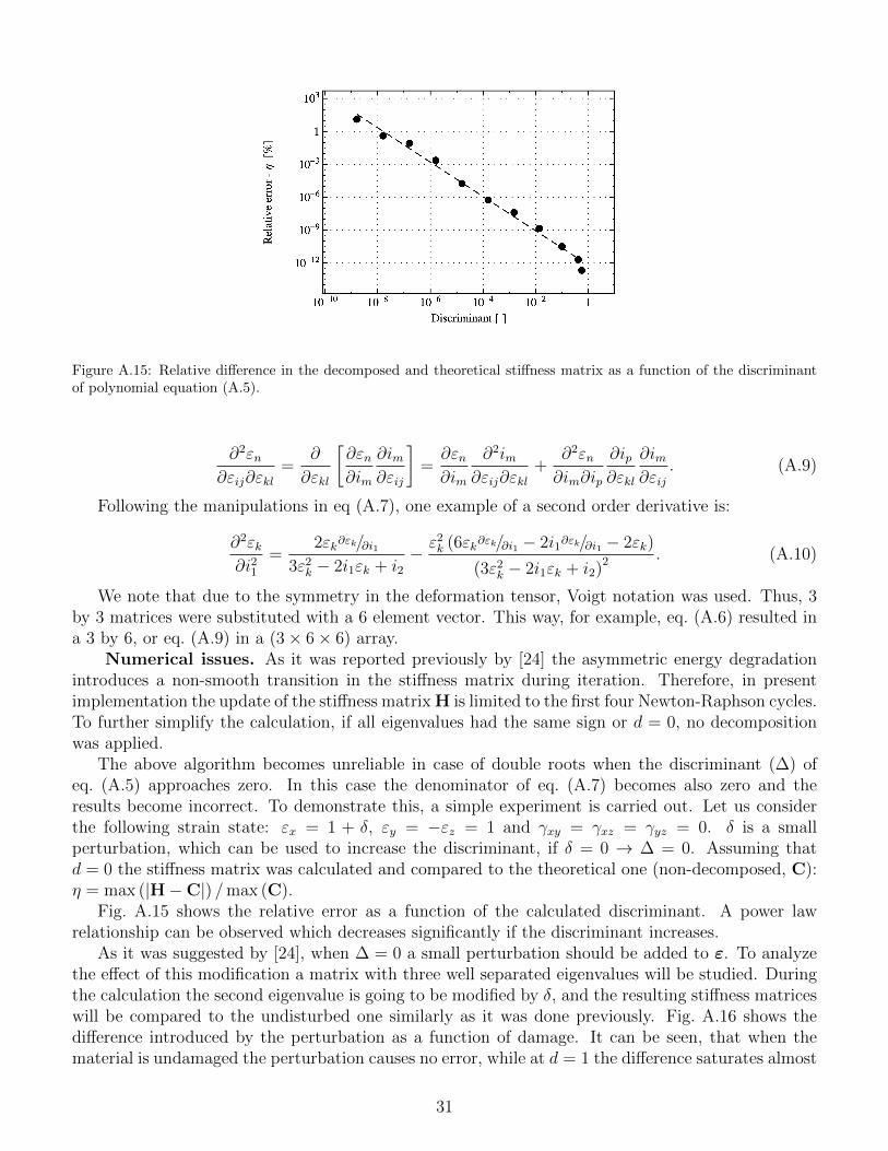
Figure A.15: Relative difference in the decomposed and theoretical stiffness matrix as a function of the discriminantof polynomial equation (A.5).

∂2εn∂εij∂εkl

=∂

∂εkl

[∂εn∂im

∂im∂εij

]=∂εn∂im

∂2im∂εij∂εkl

+∂2εn∂im∂ip

∂ip∂εkl

∂im∂εij

. (A.9)

Following the manipulations in eq (A.7), one example of a second order derivative is:

∂2εk∂i21

=2εk∂εk/∂i1

3ε2k − 2i1εk + i2

− ε2k (6εk∂εk/∂i1 − 2i1∂εk/∂i1 − 2εk)

(3ε2k − 2i1εk + i2)

2 . (A.10)

We note that due to the symmetry in the deformation tensor, Voigt notation was used. Thus, 3by 3 matrices were substituted with a 6 element vector. This way, for example, eq. (A.6) resulted ina 3 by 6, or eq. (A.9) in a (3× 6× 6) array.

Numerical issues. As it was reported previously by [24] the asymmetric energy degradationintroduces a non-smooth transition in the stiffness matrix during iteration. Therefore, in presentimplementation the update of the stiffness matrix H is limited to the first four Newton-Raphson cycles.To further simplify the calculation, if all eigenvalues had the same sign or d = 0, no decompositionwas applied.

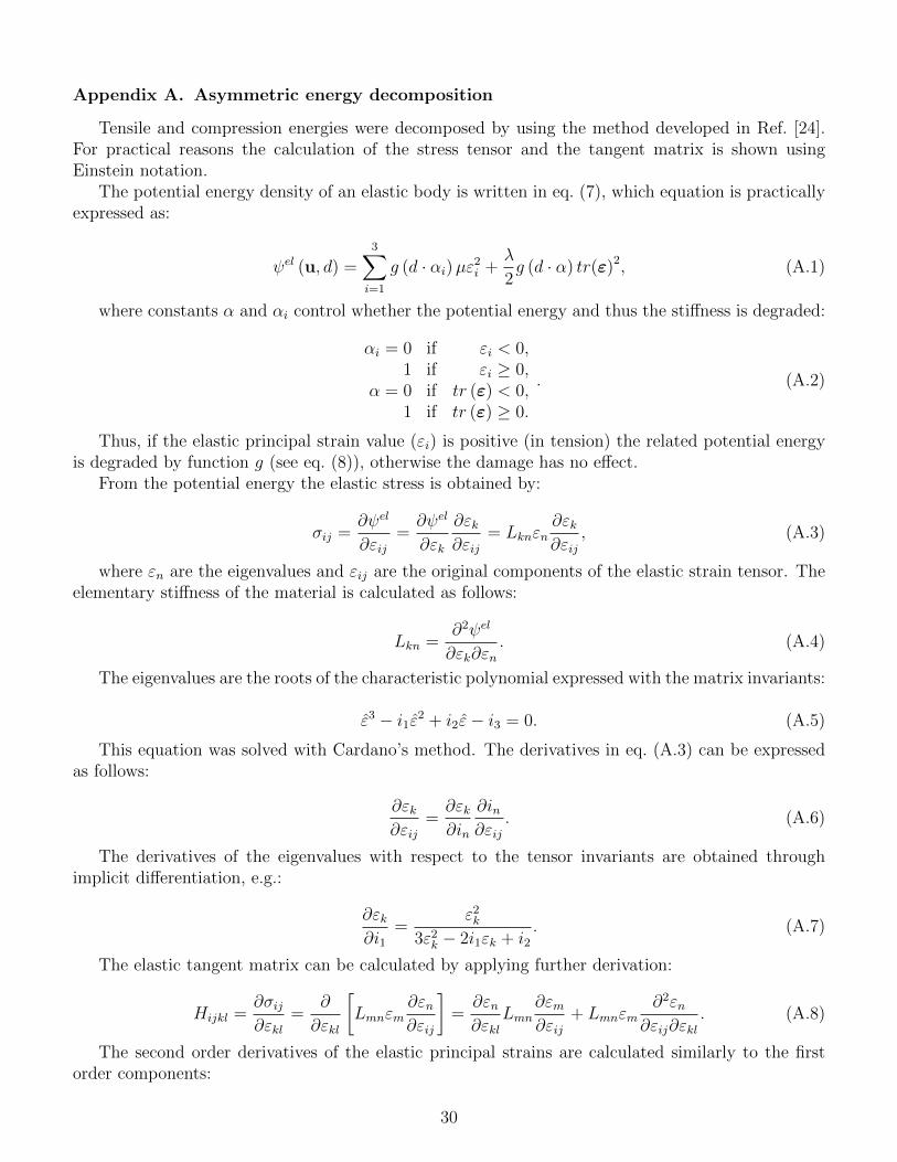
The above algorithm becomes unreliable in case of double roots when the discriminant (∆) ofeq. (A.5) approaches zero. In this case the denominator of eq. (A.7) becomes also zero and theresults become incorrect. To demonstrate this, a simple experiment is carried out. Let us considerthe following strain state: εx = 1 + δ, εy = −εz = 1 and γxy = γxz = γyz = 0. δ is a smallperturbation, which can be used to increase the discriminant, if δ = 0 → ∆ = 0. Assuming thatd = 0 the stiffness matrix was calculated and compared to the theoretical one (non-decomposed, C):η = max (|H−C|) /max (C).

Fig. A.15 shows the relative error as a function of the calculated discriminant. A power lawrelationship can be observed which decreases significantly if the discriminant increases.

As it was suggested by [24], when ∆ = 0 a small perturbation should be added to ε. To analyzethe effect of this modification a matrix with three well separated eigenvalues will be studied. Duringthe calculation the second eigenvalue is going to be modified by δ, and the resulting stiffness matriceswill be compared to the undisturbed one similarly as it was done previously. Fig. A.16 shows thedifference introduced by the perturbation as a function of damage. It can be seen, that when thematerial is undamaged the perturbation causes no error, while at d = 1 the difference saturates almost

31

Figure A.16: Relative difference in the stiffness matrices introduced by the perturbation as a function of the damagevariable. Without correction (solid symbols) and with the recalculation of the strain tensor shown in eq. (A.11).

to δ. While, this value can be reduced to δ/10 by recalculating the strain tensor based on the neweigenvalues and the original eigenvectors:

ε′ = Vε′VT (A.11)

where ε′ is the modified strain tensor, ε is a diagonal matrix containing the eigenvalues (withε′2 = (1 + δ) ε2) and V is a matrix containing the eigenvectors of ε.

As a result of these two tests, in the published implementation a small δ = 10 % perturbation isapplied on the second eigenvalue if ∆ ≤ 10−7.

Appendix B. Details of the implementation in Abaqus/UEL

To implement the solution in Abaqus two element types are used in a layered manner. Each layerconnects to the same nodes, but contributes to the stiffness of different degrees of freedom (DOF).A schematic illustration is depicted in Fig. B.17. The first element type solves the displacementproblems, hence it has 2 or 3 translational DOFs. While the second element determines the fracturetopology and has only one DOF, the phase-field.

In 2D both four-node isoparametric and three-node triangular elements are implemented. Simi-larly in 3D we considered eight-node brick and the four-node tetrahedral formulations.

In order to visualize the calculated quantities in Abaqus a third layer is added with infinitesimallysmall stiffness made from a UMAT (user defined material model). It is used to transfer informa-tion from the common block and interpolate between integration points. The internal variables aresummarized in Table B.1 for both 2D plane strain and 3D elements.

Additionally, as global history output the kinetic energy (ALLKE), the elastic strain energy(ALLIE), the plastic strain energy (ALLPD) and the fracture energy (ALLEE) is available.

The UEL option in Abaqus requires the definition of the elementary stiffness matrix and theresidue vector. In eq. (27) we gave the elementary linear equation system which is used to solve theproblem iteratively. The d’Alambert force term can be calculated as:

f ine = f inei =

∫Ω

ρNuijuidΩ, (B.1)

32

Figure B.17: 2D representation of three layered finite element structure in Abaqus. All nodes have three (or in 3Dfour) degrees of freedom (DOF). The first element contributes to the stiffness of the displacement DOFs, the secondelement to the damage DOF. For post processing purposes a third layer is included made as a UMAT model, whichallows to display state dependent variables (SDVs).

Variable Number of SDV in Abaqus

2D (x, y) 3D (x, y, z)

displacement - ux, uy, uz SDV1-SDV2 SDV1-SDV3axial strains - εx, εy, εz SDV3-SDV4 SDV4-SDV6engineering shear strains - γxy, γxz, γyz SDV5 SDV7-SDV9elastic strains - εel SDV6-SDV9 SDV10-SDV15plastic strains - εpl SDV10-SDV13 SDV16-SDV21

equivalent plastic strain - εpleq SDV14 SDV22stresses - σ SDV15-SDV18 SDV23-SDV28hydrostatic stress - tr (σ) /3 SDV19 SDV29von Mises stress - σeq SDV20 SDV30

plastic energy - ψpl0 SDV21 SDV31elastic tensile energy - ψ+

0 SDV22 SDV32potential energy - Πε SDV23 SDV33phase-field - d SDV24 SDV34

Table B.1: Solution dependent variables (SDV) used to plot the results in two and three dimensions.

33

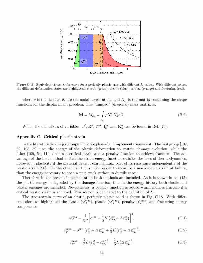
Figure C.18: Equivalent stress-strain curve for a perfectly plastic case with different Iε values. With different colors,the different deformation states are highlighted: elastic (green), plastic (blue), critical (orange) and fracturing (red).

where ρ is the density, ui are the nodal accelerations and Nuij is the matrix containing the shape

functions for the displacement problem. The ”lumped” (diagonal) mass matrix is:

M = Mkk =

∫Ω

ρNuikN

uildΩ. (B.2)

While, the definitions of variables: rd, Kd, f ext, f intn and Ku

n can be found in Ref. [70].

Appendix C. Critical plastic strain

In the literature two major groups of ductile phase-field implementations exist. The first group [107,62, 108, 59] uses the energy of the plastic deformation to sustain damage evolution, while theother [109, 54, 110] defines a critical strain and a penalty function to achieve fracture. The ad-vantage of the first method is that the strain energy function satisfies the laws of thermodynamics,however in plasticity if the material heals it can maintain part of its resistance independently of theplastic strain [98]. On the other hand it is much easier to measure a macroscopic strain at failure,than the energy necessary to open a unit crack surface in ductile cases.

Therefore, in the present implementation both methods are included. As it is shown in eq. (15)the plastic energy is degraded by the damage function, thus in the energy history both elastic andplastic energies are included. Nevertheless, a penalty function is added which induces fracture if acritical plastic strain is achieved. This section is dedicated to the definition of Iε.

The stress-strain curve of an elastic, perfectly plastic solid is shown in Fig. C.18. With differ-ent colors we highlighted the elastic (ψmaxel ), plastic (ψmaxpl ), penalty (ψmaxcr ) and fracturing energycomponents:

ψmaxel =

1

6G

[σlim +

1

2H(εcreq + ∆εcreq

)]2

, (C.1)

ψmaxpl = σlim

(εcreq + ∆εcreq

)+

1

2H(εcreq + ∆εcreq

)2, (C.2)

ψmaxcr =

1

2Iε⟨εpleq − εcreq

⟩2=

1

2Iε(∆εcreq

)2. (C.3)

34

It can be seen, that even with a large Iε there is an additional deformation component to εcreq. Forsimplicity ∆εcreq is set to 10% of εcreq. Thus, Iε is calculated as follows:

Iε =2⟨ψc − ψmax

el − ψmaxpl

⟩(∆εcreq

)2 . (C.4)

This can, of course, be changed in the UEL script when needed.Note, that if the user desires not to use the penalty function εcreq must be set to 0.

Appendix D. Recommendation for using the UEL

Abaqus proposes an alternative way, where the user can define its own element. This is called theUEL option. This section is dedicated to explain the built in options of the UEL subroutine includedin supplementary materials. With the paper a 2D plane strain and a 3D example is published.

The basic construction of the model should look like a layered finite element; where the first layeris made of elements (U1 (triangular) or U2 (square)) with translational degrees of freedom. Thisshould be followed by layer with phase-field elements (U3 (triangular) and U4 (square)) defined onthe same nodes. Finally a third layer of UMAT is recommended, which simplifies post-processing.

For the elements solving the displacement problem there are several options to consider. Theelement properties should be added in the following order: Young’s modulus (E), Poisson’s ratio (ν),yield strength (σlim), hardening modulus (H), critical strain (εcreq), thickness (only for 2D), density(ρ), asymmetric energy switch, plasticity switch, fracture surface energy (gc), internal length scale(lc). For every switch variable, the value 1 should be set if the option is used, while 0 is the it shouldbe omitted.

• Asymmetric energy switch: If the option is used, the energy is decomposed into tensileand compression parts. However, if the plastic option is applied parallel, only the hydrostaticcomponents are decomposed.

• Plastic switch: If it is used, a von Mises yield criterion is applied.

• Critical strain: If the penalty function needs to be turned off, the critical strain should be setto zero.

The fracture properties (lc and gc) are added to this element as well to control the history energyincrement and the time step.

For the phase-field element, the properties are: fracture surface energy (gc), internal length scale(lc), thickness (only for 2D), elastic threshold switch. If the elastic threshold is used ψc = gc/2lc ,else it is zero.

The element chooses automatically, if static or dynamic step integration is requested.The implemented UEL Fortran code is governed by the CeCILL-B license. The code is chosen to

be published open-source to facilitate the distribution and the ease of use of the phase-field techniqueamong Abaqus users. While on the personal website of the corresponding author (address shown inthe Fortran file), regular updates and conversion scripts are available through elaborate tutorials.

Appendix E. Supplementary data

Supplementary data associated with this article can be found in the online version at URL.

35