an simd dynamic programming c/c++ library
TRANSCRIPT
UNIVERSITY OF ZAGREBFACULTY OF ELECTRICAL ENGINEERING AND
COMPUTING
MASTER’S THESIS no. 741
An SIMD dynamic programmingC/C++ Library
Martin Šošic
Zagreb, March 2015.

I would like to thank my mentor, Mile Šikic, for his patience,
guidance and understanding. I would also like to thank my family and Anera for their
continuous support.
iii

CONTENTS
List of Figures vi
List of Tables vii
1. Introduction 1
2. SSE 3
3. Methods 53.1. Alignment methods . . . . . . . . . . . . . . . . . . . . . . . . . . . 5
3.1.1. Global . . . . . . . . . . . . . . . . . . . . . . . . . . . . . . 5
3.1.2. Local . . . . . . . . . . . . . . . . . . . . . . . . . . . . . . 5
3.1.3. Semi-global . . . . . . . . . . . . . . . . . . . . . . . . . . . 5
3.2. SWIMD . . . . . . . . . . . . . . . . . . . . . . . . . . . . . . . . . 6
3.2.1. Local alignment algorithm . . . . . . . . . . . . . . . . . . . 7
3.2.2. Additional alignment methods . . . . . . . . . . . . . . . . . 8
3.3. EDLIB . . . . . . . . . . . . . . . . . . . . . . . . . . . . . . . . . . 9
3.3.1. The basic algorithm . . . . . . . . . . . . . . . . . . . . . . . 10
3.3.2. Block algorithm . . . . . . . . . . . . . . . . . . . . . . . . 15
3.3.3. Banded block algorithm . . . . . . . . . . . . . . . . . . . . 17
4. Implementation 254.1. SWIMD . . . . . . . . . . . . . . . . . . . . . . . . . . . . . . . . . 25
4.1.1. Parallel processing of multiple database sequences . . . . . . 25
4.1.2. Core loop . . . . . . . . . . . . . . . . . . . . . . . . . . . . 27
4.1.3. Dynamic adjusting of integer precision used for alignment score 27
4.1.4. Query profile . . . . . . . . . . . . . . . . . . . . . . . . . . 30
4.1.5. AVX2 . . . . . . . . . . . . . . . . . . . . . . . . . . . . . . 30
4.2. EDLIB . . . . . . . . . . . . . . . . . . . . . . . . . . . . . . . . . . 31
iv

4.2.1. Strong reduction . . . . . . . . . . . . . . . . . . . . . . . . 31
4.2.2. Finding alignment path . . . . . . . . . . . . . . . . . . . . . 32
4.2.3. Block computation optimization . . . . . . . . . . . . . . . . 35
4.2.4. Dynamic adjustment of k . . . . . . . . . . . . . . . . . . . . 35
4.2.5. Working with undefined k . . . . . . . . . . . . . . . . . . . 35
4.3. Aligner . . . . . . . . . . . . . . . . . . . . . . . . . . . . . . . . . 38
5. Results and discussion 395.1. SWIMD . . . . . . . . . . . . . . . . . . . . . . . . . . . . . . . . . 39
5.2. EDLIB . . . . . . . . . . . . . . . . . . . . . . . . . . . . . . . . . . 41
5.2.1. Comparison with SSWL . . . . . . . . . . . . . . . . . . . . 41
5.2.2. Comparison with Myers’s implementation . . . . . . . . . . . 44
5.2.3. Comparison with Landau Vishkin . . . . . . . . . . . . . . . 45
6. Conclusion 46
Bibliography 48
v

LIST OF FIGURES
2.1. Different uasge of SSE registers and addition example . . . . . . . . . 4
3.1. Comparison of alignment methods . . . . . . . . . . . . . . . . . . . 7
3.2. Matrices C and ∆v . . . . . . . . . . . . . . . . . . . . . . . . . . . 11
3.3. Representation of ∆vj using bit-vectors . . . . . . . . . . . . . . . . 12
3.4. Deltas of four adjacent cells . . . . . . . . . . . . . . . . . . . . . . 12
3.5. Connecting inputs and outputs of adjacent blocks . . . . . . . . . . . 17
3.6. Example of banded block computation . . . . . . . . . . . . . . . . . 19
4.1. Parallel processing of multiple database sequences. . . . . . . . . . . 26
4.2. Precision adjustment - third approach . . . . . . . . . . . . . . . . . 29
4.3. Query profile . . . . . . . . . . . . . . . . . . . . . . . . . . . . . . 31
4.4. Example of alignment path . . . . . . . . . . . . . . . . . . . . . . . 32
4.5. Example of finding alignment path for NW . . . . . . . . . . . . . . 33
4.6. Finding alignment path for HW . . . . . . . . . . . . . . . . . . . . . 34
5.1. Chart comparing SWIMD with SSWL, SSEARCH and SWIPE . . . . 40
vi

LIST OF TABLES
5.1. Comparison of EDLIB with SSWL for aligning genome reads. . . . . 42
5.2. Comparison of EDLIB (NW) with SSWL with and without returning
alignment path . . . . . . . . . . . . . . . . . . . . . . . . . . . . . 42
5.3. Comparison of EDLIB (HW) with SSWL with and without returning
alignment path . . . . . . . . . . . . . . . . . . . . . . . . . . . . . 42
5.4. Comparison of EDLIB (SHW) with SSWL with and without returning
alignment path . . . . . . . . . . . . . . . . . . . . . . . . . . . . . 43
5.5. Comparison of EDLIB with SSWL for comparing proteins. . . . . . . 44
5.6. Comparison of EDLIB with Myers’s implementation . . . . . . . . . 44
5.7. Comparison of EDLIB with Landau Vishkin (SHW method) . . . . . 45
6.1. Main features of EDLIB and SWIMD compared with SWIPE and Myers. 46
vii

1. Introduction
Fast development of sequencing technologies is causing exponential growth of nu-
cleotide sequencing throughput, which is putting pressure on development of better
and faster bionformatic tools for analyzing that data.
One of the fundamental operations in bioinformatics is sequence alignment, which
can be divided to heuristic methods and deterministic methods. Deterministic methods
give optimal result of alignment but have quadratic time complexity, while heuristic
methods like BLAST [1] work much faster but give non-optimal results. Because
of their speed most aligners use heuristic methods as their main method but also use
deterministic methods to guide alignment and perform fine tuning. For example, SNAP
[2] uses Landau-Vishkin [3] as core component. Used either independently or as a part
of heuristic method, deterministic methods often prove to spend a significant amount
of CPU time.
One of the successful approaches to make deterministic methods faster is paral-
lelization using single instruction multiple data (SIMD) technology, which is supported
by most modern CPUs. Fastest SIMD implementations of Smith-Waterman-Gotoh al-
gorithm (SW) [4] [5] are Rognes’s Faster Smith-Waterman database search with inter-
sequence SIMD parallelisation (SWIPE) [6] which uses inter-sequence parallelization
and Farrar’s Striped SW (SSW) [7] with SWPS3’s [8] improvement which uses intra-
sequence parallelization. Intra-sequence parallelization is a parallelization of single
pairwise alignment (query and target), while inter-sequence parallelization is a paral-
lelization of database search (query against multiple targets). Both implementations
are significant because SWIPE is faster then SSW but SSW can be applied to more sit-
uations. There are also fast SW implementations which utilize possibilities of modern
GPUs, like SW# [9] and CUDASW++ [10].
Although deterministic algorithms are widely used and it is important that they are
efficient and fast, only few aligners use the most advanced algorithms like SWIPE and
SSW. Main reason for that is complicated implementation of those algorithms which
needs knowledge of SIMD technology and lack of adequate libraries.
1
Inspired by SSW Library [11] (SSWL) which extends on Farrar’s SSW and the lack
of sequence alignment libraries we decided to implement our own C/C++ sequence
alignment library. We implemented two libraries, SWIMD and EDLIB.
SWIPE is the fastest algorithm for database search, and therefore we decided it
would be valuable to extend it with few other alignment methods and expose as a
library. SWIMD extends on Rognes’s SWIPE, adding support for Advanced Vector
Extensions 2 (AVX2) and adding two additional semi-global alignment methods and
one global alignment method.
Although [7] is the fastest algorithm for pairwise local alignment, local alignment
is not always needed. In many cases edit distance is good enough and can be much
faster to compute, so we decided to extend from Myers’s Fast Bit-Vector Algorithm
(Myers) [12] which computes edit distance using bit-vectors and expose it as a library.
EDLIB extends on [12], adding support for finding of alignment path and adding two
additional alignment methods, one semi-global and one global.
SWIMD and EDLIB are easy to use, can be applied to any alphabet, and each of
them also comes with its own stand-alone aligner.
2

2. SSE
Streaming SIMD Extensions (SSE) is extension to the x86 architecture designed by
Intel. SSE brings 16 128-bit registers which offer SIMD operations. Each register can
contain one of following:
– four 32-bit single-precision floating point numbers
– two 64-bit double-precision floating point numbers
– sixteen 8-bit integers
– eight 18-bit integers
– four 32-bit integers
– two 64-bit integers
In order for system to support SSE, both CPU and the operating system must support
it.
SSE was later expanded with SSE2, SSE3, SSSE3, SSE4.1, SSE4.2 and lately
with AVX and AVX2. Each of this extensions brought some new instructions. Most
machines these days have at least SSE4.1, while newest machines come with AVX and
AVX2.
Since most machines support SSE, adjusting programs to utilize it (if applicable)
often brings great increase in speed. Parallelization achieved with SSE is local for one
CPU, so parallelization scales with number of CPUs.
Some of the SIMD instructions that SSE brings are addition, multiplication, shuf-
fling, shifting, bitwise operations and similar.
Except for using assembly, SSE can also be used through intrinsics. Intrinsic is a
function known by the compiler that directly maps to a sequence of one or more assem-
bly language instructions. When using intrinsics, compiler manages things like register
names, allocations and similar, which makes usage of intrinsics more convenient then
using assembly. Full list of SSE instrinsics can be found at https://software.
intel.com/sites/landingpage/IntrinsicsGuide/. Modern compilers
3

even support auto-vectorization of code, which means automatic usage of SSE regis-
ters when convenient.
Another interesting approach to using SSE is Intel SPMD Program Compiler (ISPC)
[13]. It is a special compiler created by Intel, that compiles a variant of C programming
language which has extensions for single program multiple data programming. Idea
of this language is to provide easy way to parallelize code without using intrinsics or
assembly. We tried using ISPC but it turned out that it did not provide enough control
for our needs.
AVX and AVX2 bring new 256-bit registers and new instructions that work on
them. AVX brought instructions for floating point operations, and AVX2 brought in-
structions that operate on integers. Thanks to two times larger registers, AVX and
AVX2 bring speed up of about two times over SSE.
Example of different usage of SSE registers and of SSE addition is shown on figure
2.1.
Figure 2.1: On the left, different usage of SSE registers is shown. On the right, an example of
addition is given. Next to the registers is written their intrinsic type, and next to the operation
of addition is written intrinsic that would perform such addition.
4

3. Methods
3.1. Alignment methods
When looking for the best alignment between two sequences, there are many ways
to define what exactly best alignment is and how are we going to score alignment.
Alignment method is usually chosen based on our knowledge about input data and
relation between query sequence and target sequence. Chosing different alignment
method can give very different results. In EDLIB and SWIMD, we sometimes also
refer to alignment method as "alignment mode". In this section we briefly explain
alignment methods that we implemented in SWIMD and EDLIB.
Comparison of alignment methods is illustrated in figure 3.1.
3.1.1. Global
Global alignment method is useful for detecting if two sequences of similar lengths are
similar. It tries to match both sequences completely. The most famous algorithm for
performing global alignment is the Needleman-Wunsch (NW) [14] algorithm.
3.1.2. Local
Local alignment method is useful for finding similar regions in not necessarily similar
sequences, and also for finding a shorter sequence in a longer sequence (text search-
ing). The main algorithm for local alignment is the Smith-Waterman algorithm. Local
alignment method can not be used with edit distance because there is trivial case which
always gives edit distance equal to zero.
3.1.3. Semi-global
Semi-global alignment methods are halfway between global and local alignment meth-
ods. They are used to find best possible alignment which includes start and/or end of
5

first and/or second sequence. For example, we can define global alignment method
as semi-global alignment method which includes start and end of the both sequences.
In the rest of this section we describe three semi-global alignment methods that we
implemented in SWIMD and EDLIB (names of the methods are invented):
Hybrid Needleman-Wunsch (HW)
This method includes start and end of query sequence (shorter sequence). That means
that insertions before start and after end of query sequence are not penalized. This
method is useful for finding ashorter sequence in a longer sequence.
Semi-Hybrid Needleman-Wunsch (SHW)
This method includes start and end of query sequence, and start of target sequence.
That means that insertions after end of query are not penalized. This method is useful
when we assume that query is prefix of target.
Overlap (OV)
This method includes start of one of sequences, and end of one of sequences. That
means that insertions before start of one of sequences and insertions after end of one
of sequences are not penalized. OV is useful when sequences are partially overlaping
or one of the sequences is contained in another. OV can not be used with edit distance
because there is trivial case which always gives edit distance equal to zero.
3.2. SWIMD
SWIMD extends on Rognes’s SWIPE, so in this section we describe important al-
gorithms used in SWIPE and at the same time introduce changes that were made in
SWIMD.
Main problem when parallelizing single parwise alignment is data dependency. In
order to calculate one cell in dynamic programming matrix one has to know the values
of cells above, to the left and to the up-left, which is a big constraint for parallelization.
Most basic approach for solving this data dependency is to parallelize the calculation
of one diagonal like Wozniak [15] suggested, while more efficient approach is to par-
allelize calculation of one row in a striped manner (Farrar’s SSW).
Basic idea behind SWIPE is not to parallelize single pairwise alignment, but to achieve
6

Figure 3.1: In this illustration we compare methods by showing how each method performs
when aligning each of queries AATGCCTA, CTGC and GGTAACTC against target AACTGCCT.
For scoring system we used: +1 for match, -1 for mismatch or indel. Higher the score, better
the alignment.
parallelization by performing multiple pairwise alignments at the same time. Main ad-
vantage is that there is no data dependency so parallelization is much simpler and
therefore more efficient. However, such approach is useful only when doing database
search (aligning one query against multiple database sequences).
3.2.1. Local alignment algorithm
For local alignment we use Smith-Waterman-Gotoh (SW) algorithm which uses affine
gap penalties. We have database sequence d of length n and query sequence q of
length m. In order to obtain best alignment score we have have to calculate dynamic
programming matrix H. Matrix H is created by putting database sequence along the
columns (each column is assigned to one sequence element) and query sequence along
7

the rows (each row is assigned one element from the query sequence). Hi,j is alignment
score of first i elements from q with first j elements from d. Because of Gotoh [5] we
also have to use two additional matrices, E and F, to calculate matrix H. Calculation
of matrix H is defined with the following relations:
Hi,j =
{max(Hi−1,j−1 + P [qi, dj], Ei,j, Fi,j, 0) i > 0, j > 0
0 otherwise(3.1)
Ei,j =
{max(Hi,j−1 −Q,Ei,j−1 −R) i > 0
0 otherwise(3.2)
Fi,j =
{max(Hi−1,j −Q,Fi−1,j −R) i > 0
0 otherwise(3.3)
where P is score matrix (P[qi, dj] is score of aligning qi with dj), R is gap extension
penalty and Q is sum of gap open penalty and R. Optimal local alignment score is found
by finding max Hi,j for 0 < i ≤ m and 0 < j ≤ n.
3.2.2. Additional alignment methods
In SWIPE there is only a local alignment method. In SWIMD we introduce three other
alignment methods: one global and two semi-global methods.
Global
For global alignment we use NW algorithm, together with affine gaps. It is very similar
to algorithm 3.2.1, but with few differences:
– we do not set cells in H to 0 if they reach negative value.
– we do not check every cell for potential maximal score but read optimal score
from the H[m, n].
– different boundary conditions:
H[0, 0] = 0
H[r, 0] = −Q− (r − 1) ∗R, 1 ≤ r ≤ m
E[r, 0] = −∞, 1 ≤ r ≤ m
H[0, c] = −Q− (c− 1) ∗R, 1 ≤ c ≤ n
F [0, c] = −∞, 1 ≤ c ≤ n
8

HW
HW method is very similar to global alignment that we just described, with following
differences:
– we obtain optimal score by taking maximal value from the last row of matrix
H.
– different boundary conditions at the upper edge of the matrix:
H[0, c] = 0, 1 ≤ c ≤ n
OV
OV method is also very similar to global alignment that we just described, with fol-
lowing differences:
– we obtain optimal score by taking maximal value from the last row and last
column of matrix H.
– different boundary conditions at the upper and left edge of the matrix:
H[0, c] = 0, 1 ≤ c ≤ n
H[r, 0] = 0, 1 ≤ r ≤ m
3.3. EDLIB
EDLIB extends on Myers’s Fast Bit-Vector Algorithm (Myers) [12], so in this section
we describe important concepts from Myers and also introduce additions and changes
that EDLIB brings.
Problem which EDLIB is solving is determining edit distance between given query
q of length m and target sequence t of length n. Additional property is that positive
number k can be specified, in which case edit distance is found only if it is smaller or
equal to k. If not, it will be reported that there is no such edit distance.
Edit distance is a metric for measuring the difference between two sequences.
There are few versions of edit distance but in this text we will be referring to the most
popular one, Levenshtein distance. Edit distance can be defined as a smallest number
of operations needed to change one sequence into another. Operations available are
9

insertion, deletion or substitution of element in sequence. In other words, it means that
matches are scored with 0 while insertions, deletions and mismatches are scored with
1. Opposite from the scoring system that was used in section 3.2 where larger score
was better, here the smallest score (edit distance) is the best score.
Although edit distance is not as flexible and powerful as using score matrix and
affine gaps (which we used in section 3.2), there are many applications where it is
good enough. Because of its restrictions and simplicity, edit distance has some very
interesting properties, which Myers exploited in [12] to create very fast bit-vector al-
gorithm for finding edit distance in O(kn/w) time, where w is the word size of the
machine (in number of bits, usually 32 or 64).
First we describe basic concepts from Myers but only for HW alignment method,
and next we introduce NW and SHW, which are alignment methods that we added in
EDLIB.
3.3.1. The basic algorithm
Most basic approach to finding edit distance is computing dynamic programming ma-
trix C that has m + 1 rows and n + 1 columns. Computation of C is defined with the
following relations:
C[i, j] = min
C[i− 1, j − 1] + (if q[i] = t[j] then 0 else 1),
C[i− 1, j] + 1,
C[i, j − 1] + 1
(3.4)
C[0, j] = 0 (3.5)
C[i, 0] = i (3.6)
We find optimal solution by taking minimal value from the last row of the matrix C.
Important observation is that to calculate one column, only column before is needed.
Another important observation is that the difference between adjacent cells in matrix C
is always 1, 0 or -1. We will define horizontal delta ∆h[i, j] as C[i, j]−C[i, j− 1] and
vertical delta ∆v[i, j] as C[i, j]−C[i− 1, j]. Based on this, we can transform problem
of computing C into problem of computing matrix ∆v, which is the matrix of vertical
differences between adjacent cells in C.
Both matrices and relation between them are shown on figure 3.2.
What we want is to use bit-vector operations in order to compute columns of ∆v in
O(1) time. In order to be able to do that, we will assume for a short while that m ≤ w.
We will also assume that simple operations on bit-vector like or, and, not and addition
10

Figure 3.2: Matrices C and ∆v for query throw and target bathroom are shown. In both
matrices initial conditions are colored with darkest grey. Initial conditions depend on alignment
method, which is HW in this case. Small gray circles in matrix C are vertical deltas. Small
squares on top of matrix ∆v are initial horizontal deltas (they are initial condition).
take constant time.
Since m ≤ w we consider storing one column in one bit-vector but it is not possible
because each cell in the column can have three different values. Therefore we will
represent each column with two bit-vectors, Pv and Mv. For ∆vj (j-th column) we
define two bit-vectors Pvj and Mvj with the following relations (for i ∈ [1, w]):
Pvj[i] = if ∆vj[i] = +1 then 1 else 0 (3.7)
Mvj[i] = if ∆vj[i] = −1 then 1 else 0 (3.8)
Pvj is word that has bit set when corresponding cell in ∆vj is positive (equal to 1),
while Mvj is the word that has bit set when corresponding cell in ∆vj is negative
(equal to -1). See figure 3.3 for example.
11

Figure 3.3: Representation of ∆vj = [+1,−1,+1, 0] using bit-vectors Pvj and Mvj . Bit in
Pvj is set to 1 only when corresponding cell in ∆vj equals +1, otherwise it is 0. Bit in Mvj is
set to 1 only when corresponding cell in ∆vj equals −1, otherwise it is 0.
The next important step is to find the way to efficiently calculate ∆vj from ∆vj−1.
We introduce Eq[i, j] as a bit quantity which is 1 if q[i] = t[j], otherwise it is 0.
We look at 4 adjacent cells in matrix C (two from column i and two from column i - 1)
and deltas between these cells, as shown on 3.4. There are four deltas, two horizontal
Figure 3.4: Four adjacent cells from matrix C and four deltas between them are shown on the
left picture. On the right picture is simplified drawing of relations between deltas: ∆v[i, j]
(∆vout) and ∆h[i, j] (∆hout) can be computed from Eq[i, j] (Eq), ∆v[i, j − 1] (∆vin) and
∆h[i− 1, j] (∆hin).
and two vertical deltas: ∆v[i, j], ∆h[i, j], ∆v[i, j − 1] and ∆h[i− 1, j].
Using definition of deltas and relation 3.4, we can express ∆v[i, j] and ∆h[i, j] in terms
of Eq[i, j], ∆v[i, j − 1] and ∆h[i− 1, j] (see [12] for more details):
∆v[i, j] = = min(−Eq[i, j],∆v[i, j − 1],∆h[i− 1, j]) + (1−∆h[i− 1, j]) (3.9)
∆h[i, j] = = min(−Eq[i, j],∆v[i, j − 1],∆h[i− 1, j]) + (1−∆v[i, j − 1]) (3.10)
Because of this relations, we can look at ∆vin = ∆v[i, j− 1], ∆hin = ∆h[i− 1, j] and
12

Eq = Eq[i, j] as inputs to computation, and at ∆vout = ∆v[i, j] and ∆hout = ∆h[i, j]
as outputs.
Next observation is that ∆vin and ∆hin each can have three possible different val-
ues, and that Eq can have two possible different values. Therefore there are only
3 ∗ 3 ∗ 2 = 18 different inputs when computing ∆vout and ∆hout.
We define Pvin and Mvin as bit values representing ∆vin, in the same fashion like
defined before for ∆vj . Analogous to that, we also define Pvout, Mvout and corre-
sponding terms for horizontal deltas. Next, studying possible combinations of inputs
and their outputs, we define relations for computing ∆vout and ∆hout in somewhat dif-
ferent manner, using auxiliary bit values Xv and Xh and representing delta values using
defined bit values:Xv = Eq or Mvin
Pvout = Mhin or not (Xv or Phin)
Mvout = Phin and Xv
(3.11)
Xh = Eq or Mhin
Phout = Mvin or not (Xh or Pvin)
Mhout = Pvin and Xh
(3.12)
In order to be able to calculate next colum in matrix ∆v, we need to know the
Boolean value Eq for each cell. Since we are working with bit vectors, we need Eq
values also stored in bit vectors. Doing that for each column while computing matrix
∆v would slow us down significantly since we want to be able to calculate one column
in O(1) time.
Luckily, we can exploit the fact that alphabet has finite size and construct all needed bit
vectors containing Eq values in preprocessing step. We build array Peq which is the
same size like alphabet, and whose elements are defined with the following relation,
where s is symbol from alphabet:
Peq[s][i] = (if q[i] = s then 1 else 0) (3.13)
For calculating ∆vj we will use Peq[t[j]].
To actually be able to find the optimal score (edit distance), we need an efficient
way to calculate one column (∆vj) from previous column (∆vj−1). When calculating
column ∆vj we will actually be calculating Pvj , Mvj and Scorej . Input to this calcu-
lation are Pvj−1, Mvj−1, Scorej−1, t[j] (using which we obtain Peq[t[j]]) and initial
13

horizontal delta ∆h[0, j] which is initial condition. Initial conditions are:
Pv0 = [1, ..., 1]
Mv0 = [0, ..., 0]
Score0 = m
∆h[0, j] = 0, 1 ≤ j ≤ n
(3.14)
To calculate vertical deltas of the new column (∆vj) using relations 3.11, we need
to know horizontal deltas for that column (∆hj).
Therefore we will split our computation in two steps: first step is to compute horizontal
deltas using relations 3.12, and second step is to compute vertical deltas using relations
3.11. When first step is finished, we will shift horizontal deltas down, pushing last
horizontal delta out and putting inital horizontal delta as first. Last horizontal delta,
which we just pushed out, we will use to update the Score.
Obvious problem here is that, in first step, to calculate one horizontal delta we need
horizontal delta above, which means we would have to calculate them one by one
which takesO(m) time and we needO(1) solution. For now we will solve this problem
by assuming that we can compute Xh in O(1) time, and later we will show how this
can be done.
Using relations 3.11 and 3.12 we obtain following formulas that describe compu-
tation of a new column:
Phj[i] = Mvj−1[i] or not (Xhj[i] or Pvj−1[i])
Mhj[i] = Pvj−1[i] and Xhj[i](3.15)
Scorej = Scorej−1 + (1 if Phj[m])− (1 if Mhj[m])
Phj[0] = Mhj[0] = 0(3.16)
Pvj[i] = Mhj[i− 1] or not (Xvj[i] or Phj[i− 1])
Mvj[i] = Phj[i− 1] and Xvj[i](3.17)
Formulas 3.15 (step 1) and 3.17 (step 2) describe computation of bits in bit vectors.
However, we do not calculate bit by bit, instead we calculate all of them in parallel
using bitwise operations on bit vectors.
In formulas 3.16 we describe work that is done in between steps. When we set initial
horizontal delta by setting Phj[0] and Mhj[0] to 0, it is important to notice that this
operation depends on the value of initial horizontal delta. In this case initial horizontal
14

delta is always 0 because we are using HW alignment method, however if horizontal
delta was not 0 but had some different value (because we were using some other align-
ment method or block version of algorithm), we would have set Phj[0] and Mhj[0]
accordingly.
Computing Xh
Before we assumed that we can computeXh inO(1) time, and in this section we show
how. Problem is that to compute Xhj we need Mhj , and to compute Mhj we need
Xhj . By unwounding this cyclic dependency and determining a way to compute it in
constant time using bit vectors as shown in Myers [12], we get the following formula:
Xhj = (((Peq[t[j]] & Pvj−1) + Pvj−1) ˆ Pvj−1) | Peq[t[j]] (3.18)
where &, | and ^ are bitwise operators AND, OR and XOR, respectively. What this
formula actually does is: when there is a bit set in Eq (at position i), it also sets that
bit in Xh, and it also sets k next higher bits in Xh if there is a run of k set bits in Pv
starting with i-th bit. Important thing to mention here is that formula above works only
for HW alignment method. In order to work correctly for other methods, Peq[t[j]][1]
should be set to 1 if Mhj[0] is set to 1 (this is because of initial horizontal delta).
We have shown that using bit vectors we can calculate new column in constant
time. However, we do not have access to individual cells in matrix (because that would
ruin constant time of computation) but only to outputs of blocks. We do have access to
score of the last cell in a block, which is represented as Score output. Time complexity
of this basic algorithm is O(mσ + n) (O(mσ) is complexity of building Peq, and
O(n) is complexity of calculating columns of matrix ∆v), and space complexity is
O(σ) (since one column can fit in one word).
3.3.2. Block algorithm
Algorithm that we described in section 3.3.1 is usable only when length of query is
not larger then the length of the word (m ≤ w). In this section we extend the basic
algorithm so it can be used with queries of arbitrary length, and then we extend that
algorithm to banded block algorithm that will use blocks but calculate only a portion
of dynamic programming matrix.
If we have a query of length m that is larger then word length w, then whole matrix
column does not fit in one bit vector. We solve this problem by splitting each column
15

into blocks of size w. Therefore, each column contains B = dm/we blocks, and our
dynamic programming matrix is transformed into B × n matrix of blocks. Time com-
plexity of this algorithm isO(mσ+dm/wen), while space complexity isO(dm/weσ).
We can calculate blocks either column by column, row by row, or diagonal by
diagonal, since for each block we need block above and block to the left to be already
calculated. We calculated them column by column since it is simpler then by diagonals,
and it takes less memory to store last column (B blocks) then last row (n blocks) since
query is usually much smaller than target and blocks are oriented vertically.
We also adjust Peq: since there are B blocks in one column, Peq[σ] no longer
contains bit vector but array that contains B bit vectors, each for one block.
If m is not a multiple of w then last block will have W = w− (m mod w) too many
cells. We solve this by padding query sequence with W wildcard characters. Wildcard
characters are special characters which match with all other characters from alphabet.
We support this when building Peq by always setting bit to 1 when wildcard in query
is encountered, regardless of element from target.
Because of padding that we introduced, Score of last block in column will no longer
hold correct value if W > 0. Instead, its Score contains Score of block that is W
positions to the left. That means that Scores of blocks in the last row are shifted to
the right for W positions. Having this in mind we can easily obtain correct scores,
however last W scores are lost because of shifting. We can solve this either by also
padding target with W wildcards (as suggested in [12]) or by going manually through
last W cells(bits) of last block in last column. First approach is somewhat simpler,
but second approach is more efficient and that is what we used in implementation of
EDLIB. Padding using second approach is illustrated in figure 3.6.
Initial horizontal deltas
In basic algorithm, one of inputs to a new column(block) was initial horizontal delta
(also called input horizontal delta), which was defined by the alignment method that
we were using (and it was always 0 for HW). This was valid because all blocks were
starting at the upper boundary of matrix. In our block based algorithm not all blocks
start at the upper boundary of matrix and such blocks will for their initial horizontal
delta use last horizontal delta of the block above. On figure 3.5 is illustrated how we
connect inputs and outputs of adjacent blocks.
As said before, if we are using HW as alignment method, initial horizontal deltas
at top boundary are always 0. However, if we use SHW or NW, then those initial
16

Figure 3.5: Connecting inputs and outputs of adjacent blocks. Last horizontal delta of block
above becomes first horizontal delta for new block. Vertical deltas of block to the left become
input vertical deltas for new block.
horizontal boundaries will not be 0 but always 1.
Important thing to notice is that input horizontal deltas may be +1, 0 or -1, and
we should keep this in mind while applying algorithms described in 3.3.1 as there are
some modification that need to be done in such case (all of them were mentioned and
described).
3.3.3. Banded block algorithm
Next, we extend from block algorithm to banded block algorithm. Main idea behind
banded algorithms is to determine which cells are certainly not part of solution, and
then not compute that cells. One of most popular banded algorithms is Ukkonen’s
Algorithms for Approximate String Matching [16]. We define band as span of adjacent
cells/blocks of one column such that all cells/blocks that are outside of band (above
or beneath it) are certainly not part of solution. Therefore, we represent band for one
column as pair of integers (firstB, lastB) where firstB is index of first cell/block in
band, and lastB is index of last cell/block in band.
Usually, banded algorithms are provided with parameter k, which is upper limit
for best solution. In other words, only solutions not bigger then k will be explored.
Algorithm that we are going to describe also takes parameter k.
There are different approaches to determining band. One approach is to determine
band of cells that are to be computed in advance, based on k. This is obviously not
17

optimal since during computation of matrix we obtain some information that we will
not be using.
Somewhat more complicated approach is to also adjust band during computation, us-
ing values of computed cells to determine if band should be narrower/wider. Although
better guided, in this approach it is important to be careful not to spend to much re-
sources on adjusting the band (if we spend too much time trying to adjust the band, it
may negate the benefits of adjusting it).
We have chosen second approach, and will adjust band each time after column
has been computed. While, like we mentioned before, adjusting band each time after
column has been computed may be too expensive (time consuming), it is actually very
convenient since we use blocks, not cells. Since we use blocks, we can not easily
access individual cells inside one block. However, we do know the value of last cell
in each block as it is stored in Score. This does provide us with less information to
adjust the band, but it also makes adjustment of band faster (since we deal with lot less
information to process), and therefore makes this approach the best choice.
When calculating new column, it can happen that we are computing block b whose
left neighbour we never computed, because it was outside of previous column band.
In that case we have to determine what will we use as input for block b. Since we
know that block to the left is not part of solution and that it is not really important
for calculation of block b, we put the most pesimistic input possible (which is when
all ∆vs are equal to 1). By doing this, we ensure that no score in cells in block b is
obtained by advancing from cells from block to the left.
Example of banded block computation is shown in figure 3.6.
When we compute new column, we use band from the previous column. Then we
adjust the band, and in case it becomes wider, we calculate that one more block (it
will never grow for more then one block). It is important to notice here that index of
first block in band can only increase, while index of last block can both increase or
decrease. This new band is then used to compute next column, and so on.
Time complexity of the banded block algorithm isO(kn/w), and space complexity
is same like for the block algorithm, O(dm/weσ).
Although they are all based on the the same approach, we use different algorithms
for adjusting the band depending on the alignment method. Blocks and cells are 1-
indexed (first block/cell has index 1).
18

Figure 3.6: Example of banded block computation where B = 2, w = 4, W = 2 and we are
using SHW alignment method. Cells marked with x are cells that are part of solution (that are
inside band). Blocks that have at least one cell that is inside band are also inside band, and are
colored gray. Cells with wave pattern are padding cells. Sj label represents score of column
j that propagates from the last row of matrix. All scores are shifted two cells down and two
cells to the right. Thick left boundary of block with label 1* represents input where all vertical
deltas equal 1, which is used when block to the left was not computed.
Band adjustment for HW and SHW
We created this algorithm by extending from algorithm in Myers [12] and introducing
some changes.
For HW and SHW, cell is not part of solution if its value is greater than k. There-
fore, we will say that block is outside of band if all its cells have value greater then
k.
Initial band Band for first column is set to (1,min(d(k + 1)/we, B)). First block
of band is set to first block in column, and last block of band we determine based on
the fact that the first cell of first column is always 0, and every next cell is bigger then
previous cell for 1. That means that i-th cell has value i−1 and that we want first k+1
cells in our band, therefore the formula above.
One simple condition that we can use to detect if computed block is outside of band
19

is following:
Score ≥ k + w (3.19)
Here we should remember that Score is value of last cell in block. If this condition is
satisfied, then block is certainly outside of band. If not, then we can not say for sure if
block is outside of band of not, so we ussualy assume it is.
Idea behind this is that although we know only value of last cell, we also know that
difference between two adjacent cells is always +1, -1 or 0. Therefore, the smallest
value first cell in block can possibly have is Score − w + 1, and other cells will also
not have smaller value then that. Block is outside of band if all cells are outside of
band, which means that each cell has to satisfy condition s > k where s is value of
cell. Since we know that for each cell in block statement s ≥ Score − w + 1 is
correct, combining it with condition s > k we get that block is outside of band if
Score− w + 1 > k. By reshaping this condition a bit, we get condition 3.19.
Next we are going to explain how we adjust the band after new column has been
computed.
Adjusting first block We adjust first block of band only for SHW, because HW has
such initial conditions that first block is always part of solution. First block is adjusted
by checking the condition 3.19. As long as the condition is satisfied, we increase index
of the first block in band for one.
Adjusting last block Concerning the last block in band, first we check if band can
be increased for one block. We do this by using condition from Myers:
(Score−∆hout ≤ k) and ((PeqNext & 1) or ∆hhout < 0) (3.20)
where Score and ∆hout are outputs of last block, and PeqNext is entry from Peq for
block below. The idea behind this condition is to check first cell of new block could
have value that is not greater then k. If condition is satisfied, we increase index of last
block for one and calculate this new block.
After we tried to increase the index of last block in band, next we try to reduce it. Same
like we did with the first block, we decrease index of last block in band for one as long
as condition 3.19 is satisfied for it.
Band adjustment for global alignment (NW)
Following algorithm is not from [12] but was created by us.
20

Important difference between global alignment and semi-global alignment is that
solution for global alignment (NW) must reach last cell in last column of dynamic pro-
gramming matrix, while in semi-global alignment methods last cell of any column can
be the solution. Therefore, we can introduce much stricter conditions for determining
if a block is outside of band.
We define conditions that define which cells are in band.
We define S(r, c) as value of cell from row r and column c.
We also define S ′(r, c) as optimal score when aligning last m − r characters of query
with last n − r characters of target. After we have computed cell (r, c) we still do
not know value of S ′(r, c), but we can determine its lower limit. We can easily see
that lower limit for S ′(r, c) is achieved when there are only matches (no mismatches)
and we move diagonally until we hit the boundary (bottom or right) of matrix. Then
we move along the boundary until we reach the last cell of last column in matrix.
Therefore, we get the following lower limit:
S ′(r, c) ≥ |(n− c)− (m− r)| (3.21)
Last, we define S ∗ (r, c) as best solution for aligning query and target such that cell
from row r and column c is part of solution. We can easily notice following:
S∗(r, c) = S(r, c) + S ′(r, c) (3.22)
As we said before, cell is part of band if it is part of final solution that is not larger than
k. Therefore, cell (r, c) must satisfy condition
S∗(r, c) ≤ k (3.23)
in order to be inside band. If this condition is not satisfied, cell is out of band.
Combining equations above, we get the following:
S∗(r, c) ≤ k
S(r, c) + S ′(r, c) ≤ k
S(r, c) + |n− c− (m− r)| ≤ k
|n− c−m+ r| ≤ k − S(r, c)
In order for last line to have a possible solution, right side must be non-negative, so we
continue with assumption that S(r, c) ≤ k. This is actually the basic condition, since
21

cell is certainly not in band if its score is larger then k.
S(r, c)− k ≤ n− c−m+ r ≤ k − S(r, c)
S(r, c)− k − n+m+ c ≤ r ≤ k − S(r, c)− n+m+ c
Finally, we can say that cell (r, c) is inside band if and only if three following
conditions are met:
S(r, c) ≤ k (3.24)
r ≥ S(r, c)− k − n+m+ c (3.25)
r ≤ k − S(r, c)− n+m+ c (3.26)
What we need is, after we computed specific column, to determine which cells in
it are in/out of band. Obviously, equations 3.25 and 3.26 represent boundaries of band.
Adjusting first block We describe how to adjust first block of band. We are in-
terested in detecting cells that are above band, and that are cells that do not satisfy
equations 3.24 or 3.25. In other words, that are cells that satisfy at least one of the
following equations:
S(r, c) > k (3.27)
r < S(r, c)− k − n+m+ c (3.28)
However, we know only value of last cell in each block, which is Score. Therefore, we
adjust equations 3.27 and 3.28 so they become applicable to blocks.
As already shown in section 3.3.3, condition 3.27 is met for whole block when condi-
tion 3.19 is met.
Next, we notice that if condition 3.28 is met for the last cell in block, it is also met for
all other cells in block. We can prove this easily: let r’ be row and Score’ be score of
some cell from block whose last cell satisfies condition 3.28 and rlast be row of the last
cell in block:
r′ = rlast −∆r
rlast < Score− k − n+m+ c
From above, we get following:
Score′ ≥ Score−∆r
r′ + ∆r < Score′ + ∆r − k − n+m+ c
r′ < Score′ − k − n+m+ c
22

which shows that condition 3.28 is met for all cells in block (actually, for all cells in
the column for which r ≤ rlast), if it is met for last cell in block.
Therefore, we get the following rule for adjusting first block:
While condition
(Score ≥ k + w) or (rlast < Score− k − n+m+ c)
is met, increase index of first block in band for one.
Adjusting last block We describe how to adjust last block of band. We are interested
in detecting cells that are below band, and that are cells that do not satisfy equations
3.24 or 3.26. In other words, that are cells that satisfy at least one of the following
equations:
S(r, c) > k (3.29)
r > k − S(r, c)− n+m+ c (3.30)
Again, we have to adjust this equations to work for blocks. We already know how to
adjust equation 3.29, so we only have to adjust equation 3.30.
We address score of first cell in block as Scorefirst, and its row as rfirst. We notice that
if condition 3.30 is met for the first cell in block, then it is also met for all other cells
in block (actually, for all cells in the column for which r ≥ rfirst). Proof is analogous
to the one for adjusting first block, so we will not write it here.
However we do not know the value of first cell in block, so we express the condition
rfirst > k − Scorefirst − n + m + c using last cells of blocks (we define ScoreprLastas score of last cell in block above):
rfirst = rlast − w + 1
Scorefirst ≥ max(ScoreprLast − 1, Score− w + 1)
rfirst > k − Scorefirst − n+m+ c
rlast − w + 1 > k −max(ScoreprLast − 1, Score− w + 1)− n+m+ c
rlast > k −max(ScoreprLast − 1, Score− w + 1)− n+m+ c+ w − 1
Therefore, we get the following rule for adjusting the last block:
While condition
(Score ≥ k + w) or (rlast > k −max(ScoreprLast − 1, Score− w + 1)− n+m+ c+ w − 1)
is met, decrease index of last block in band for one.
However, before trying to narrow the band, we should try to make it bigger. We do
23

this by checking if last block satisfies the condition above, if not then we increase the
band for one block and compute it. After that, we try to decrease index of last block as
described above.
Initial band Before we start computing dynamic programming matrix, we have to
determine initial band size that will be used for first column. We start from S∗(r, c) ≤ k
but apply c = 1 and use fact that S(r, 1) = r − 1:
S∗(r, 1) ≤ k
r − 1 + |n− 1−m+ r| ≤ k
|n− 1−m+ r| ≤ k − r + 1
In order for last line to have a solution, right side must be non-negative, so we continue
with assumption that r ≤ k + 1:
r − k − 1 ≤ n− 1−m+ r ≤ k − r + 1
−k ≤ n−m ≤ k − 2r + 2
Therefore, we get that first column band contains all cells for whom all following
conditions are satisfied:
r ≤ k + 1
m− n ≤ k
r ≤ 1
2(k + 2 +m− n)
We notice that another condition that has to be met in order for solution to exist is that
k > |m− n|. Combining this with above, we get that solution exists only if condition
k > |m− n| (3.31)
is met, and in that case band for first column is defined as(1,
⌈min
(k,⌊12(k + 2 +m− n)
⌋)w
⌉)(3.32)
24

4. Implementation
When implementing SWIMD and EDLIB, we focused on speed but also on usabil-
ity. Both were implemented as C/C++ libraries and were developed and tested on
Linux(Ubuntu). Both libraries are public and are available online as git reposito-
ries. SWIMD is available at http://github.com/Martinsos/swimd, while
EDLIB is available at http://github.com/Martinsos/edlib.
Both SWIMD and EDLIB can work with any alphabet given.
4.1. SWIMD
For utilizing SIMD technologies we used Intel intrinsics, which are available through
immintrin.h. All scores in SWIMD are integers, so we used data type __m128i
and intrinsics that work with integers.
Library is simple to use and exposes only one function: swimdSearchDatabase.
swimdSearchDatabase takes following input: query sequence, database sequences,
gap open penalty, gap extension penalty, score matrix, length of alphabet, alignment
method(mode). It is interesting to note here that sequences are not given as arrays of
characters, but as arrays of indices of characters in alphabet. Output is array of scores,
one for each database sequence.
AVX2 is recognized by EDLIB and is automatically used if available, if not SSE4.1
is used.
4.1.1. Parallel processing of multiple database sequences
We process multiple database sequences at once using SSE vectors. Depending on
integer precision that we use for alignment score, SSE vector is divided into N fields
(N = 4 for int(32 bits), N = 8 for short(16 bits) and N = 16 for char(8 bits)).
At the beginning we assign each of N sequences to one field in SSE vector. At each
iteration we simultaneously calculate one cell in dynamic programming matrix of each
25

sequence. Therefore, we calculate N dynamic programming matrices at once. Calcu-
lation is done column-wise (column by column), and when one column is calculated
each sequence is advanced for one element. When one sequence reaches its end, it
is replaced by the next sequence from the database: next sequence is assigned to the
same field to which old sequence was assigned before.
This process is illustrated by 4.1.
Figure 4.1: In this illustration of parallel processing of multiple database sequences N is 4
and sequences are already assigned to vector fields. Left picture shows SSE vector with 4
sequences. Already processed elements are marked with X, while elements currently being
processed are marked with their index in sequence (which is also index of column in matrix),
starting from 1. Right picture shows corresponding dynamic programming matrices. Third row
is currently being processed, and those cells are colored in darker gray. Cells are labeled with
their row and column indices, both starting from 1.
If we did not use parallelization, for calculation of one cell from H we would need
following: value of cells from H that are to the left, up and up-left, value of cell from
F that is above and value of cell from E to the left. That means we have to keep in
memory previous columns of matrices H and E and value of previous cell from matrix
F.
We use parallelization, so instead of a cell we use an SSE vector. Therefore, we keep
in memory at all times two arrays of SSE vectors (columns from H and E) and one
SSE vector that contains values of previous cells from matrix F.
We can notice that with this kind of parallelization, calculation is basicaly the same
like in the section 3.2.1, only difference is that we work with SSE vectors(which con-
tains N cells) instead of cells and therefore we have N-fold parallelization.
26

4.1.2. Core loop
Core part of our computation is calculating new cell in matrix H using relations from
section 3.2.1. Of course we do not work with cells, but with SSE vectors instead.
Below is the pseudocode of core loop:
E = max(prevHs[r] - Q, prevEs[r] - R);
F = max(uH - Q, uF - R);
H = max(F, E);
H = max(H, vector_0);
ulH_P = ulH + P[query[r]];
H = max(H, ulH_P);
maxH = max(maxH, H); // update best score
uF = F;
uH = H;
ulH = prevHs[r];
// Update prevHs, prevEs in advance for next column
prevEs[r] = E;
prevHs[r] = H;
Variables R, F, H, ulH_P, ulH, uF, uH and maxH are SSE vectors, while prevHs and
prevEs are arrays of SSE vectors. r is index of current row, while P is column from
query profile that corresponds to current column.
4.1.3. Dynamic adjusting of integer precision used for alignmentscore
To achieve largest factor of parallelization we use 8-bit integer (char) to store our scores
and perform calculations. Using 8-bit score and 128-bit SSE vector we can process 16
database sequences at once (N = 128/8 = 16).
For SW mode we do not use all 8 bits but only 7 bit range from -128 to -1 (we bias
all scores by an offset of 128). Although this reduces our range in half, it ensures that
signed saturation and addition work well for the SW (score never becomes negative
so we do not have to set score manually to zero when negative). Also, usage of neg-
ative range enables the usage of add and subtract signed saturated bytes instructions
which are very fast. We tried using both 8-bit range and 7-bit range and 7-bit range
displayed better performance. For other modes we use 8-bit range because their score
can become negative.
27

Problem with using certain precision occurs when score exceeds upper limit of
precision and overflow happens. In that case we have to detect overflow and increase
precision. In SWIPE they use 3 different precisions: 7 bit, 16 bit and 63 bit while
we use 7(8) bit, 16 bit and 32 bit. We use 32 bit because it gives us bigger factor of
parallelization then 63 bit, and we found 32 bits to have range big enough.
First approach we tried is to save state of computation for database sequences
at which overflow occurred and, when all database sequences have been processed,
switch to higher precision and continue calculation of database sequences that over-
flowed (we can continue their computation because we saved their state). However,
saving and then restoring the state of the sequences proved to be too expensive and
made the whole approach inefficient.
Second approach that we tried was similar to first, but without saving state. If
computation for some database sequence overflowed, we would repeat its calculation
with higher precision but from beginning. This approach is used in SWIPE, and it
performs better then first approach because amount of the time lost on saving and
loading state is usually bigger then amount of the time lost when repeating calculation
from beginning.
However, we can notice that range in which score will be and therefore precision
that we need to use depends on scoring system (scoring matrix and gap penalties) and
properties of database sequences.
We also notice that if scoring system mostly contains large values, scores will be high
and larger precision will be needed. In such case the second approach will do a lot
of unneeded computation, since lower precision will not be of much use. For global
and semi-global modes, if database sequences are not similar to query or are of very
different size then query, score will be highly negative and higher precision might be
needed. In that case the second approach will again do a lot of unneeded computation
because it will try to calculate all of sequences using lower precision first, and then
switch to higher precision.
Trying to solve the problems listed above, we implemented third approach. In the
third approach database is divided into chunks of equal size and we compute chunk
by chunk. We start to compute sequences from a chunk using lowest precision until
overflow in one of the sequences is detected. When overflow is detected we switch
to higher precision, repeat computation for sequence that caused overflow and com-
pute all sequences in the chunk that were not computed yet. That way, if most of
sequences require higher precision, only small amount of sequences will be calculated
using lower precision because we will switch to higher precision very soon. Division
28

into chunks gives us chance to switch back to lower precision. This approach is more
robust towards scoring system and properties of database sequences and also proved to
be most efficient, so this is approach that we use in SWIMD.
Approach is illustrated in figure 4.2.
Figure 4.2: In this example of precision adjustment using third approach there are three
chunks, each containing 4 database sequences. Sequences are labeled with numbers which
represent lowest precision that is sufficient to compute that sequence without overflow (when
doing calculation this is not known). Three horizontal lines represent precision that was used
to compute certain database sequence. Arrow means that overflow was detected and precision
was increased.
Overflow detection
There is no mention of overflow detection in SWIPE, so we introduce overflow detec-
tion that we used in SWIMD. To detect overflow we use several techiques, depending
on precision and alignment mode that we use. Although overflow happens inside the
core loop, we do not want to check for it in the core loop because we want to keep the
core loop small and fast. Therefore we do as little work about detecting overflow in
the core loop as possible (mostly save some state), and then check for overflow when
one column is calculated.
Saturation arithmetic is a version of arithmetic where result of all operations like
subtraction and addition is limited with minimum and maximum value. If result of
operation goes over the limit, it is set to that limit (for example, with range 0 - 255, we
have 100 + 180 = 255). Saturation arithmetic is supported by SSE for certain types, so
we use it when possible as it simplifies overflow detection.
If using saturation arithmetic it is easy to check for overflow: in core loop we save
most outstanding values and then if any of them is equal to upper/lower limit we say
we detected overflow (this reduces score range by two which is insignificant).
When not using saturation arithmetic, we make assumption that gap penalties and
all scores in score matrix are between lower_range / 2 and upper_range / 2. We check
for this condition when starting calculation and if condition is not met, we increase
29

precision. By keeping track of minimal score that occured in core loop we can later
detect overflow by checking if that minimal score is smaller than lower_range / 2.
Only case for which we do not do overflow detection is when using highest preci-
sion of 32 bits, as we do not expect scores to be outside of 32 bit range.
4.1.4. Query profile
When doing computation of matrix H without parallelization, in order to calculate new
cell we need value of P[q[r], d[c]] where r is index of current row, c is index of current
column and P is score matrix.
Since we work with vector of N cells, we build vector PB of values P[q[r], di[ci]] for
1 ≤ i ≤ N where di is database sequence currently assigned to field i of SSE vector
and ci is index of current column for that sequence (column that is currently being
processed). Building such vector is expensive and we want our core loop to be as fast
as possible, so we are going to solve this problem by building query profile (QP).
We can notice that while calculating one column, only r changes. qr is element of al-
phabet, which means that for this column there will at most alphabet_length different
PB vectors, therefore many of PB vectors will be identical. Every time when we move
to a new column (when current database sequences advance for one element) we build
QP by building PBs for all possible values of qr combined with values of di[ci] for
1 ≤ i ≤ N which are fixed for this column. That way we get an array of SSE vectors
called QP where, if we look at it as a table where vectors are rows, rows are labeled
with elements of alphabet and columns are labeled with currently being processed el-
ements of current sequences. Now, when q[r] = e we read needed PB from QP[e].
Assuming query is much larger then alphabet length, we can see that building QP for
each column is much more efficient then calculating each PB in core loop. Illustration
of QP is shown in figure 4.3.
4.1.5. AVX2
SWIMD needs at least SSE4.1 to work, but we also added support for AVX2 (which
SWIPE does not have).
AVX2 brings 256-bit registers which means that we can process double the amount
of database sequences that we could process with 128-bit registers, therefore using an
8-bit precision, we can process 32 database sequences at once!
During compilation, we detect if SWIMD was compiled for AVX2 by checking if
macro __AVX2__ is defined. If yes, instead of 128-bit SSE types and intrinsics we
30

Figure 4.3: On the left is shown query profile for alphabet ACTGN, query GCG (for the simplic-
ity of example query is shorter then alphabet, but normally query will be longer then alphabet)
and 4 database sequences (N = 4) whose currently being proccesed elemets are C, T, A and C.
Shown query profile is array that contains 5 SSE vectors (because alphabet length is 5), each
of them containing 4 elements (because N is 4). As show on the right picture, when calculating
first and third row of matrix H, fourth SSE vector from query profile is used, while for the
second row second SSE vector from query profile is used.
use corresponding 256-bit types and intrinsics. AVX2 is needed and not just AVX
because AVX2 brings full support for integer operations on 256-bit vectors. If AVX2
is not supported, then we check if macro __SSE4_1__ is defined. If yes, 128-bit SSE
types and instrinsics are used, otherwise error is thrown.
4.2. EDLIB
In EDLIB we perform SIMD operations by using normal registers as bit-vectors.
There is only one function exposed by library: myersCalcEditDistance.
Input of myersCalcEditDistance is: query, target, length of alphabet, k, align-
ment method(mode), whether to find alignment. Output is score, position in target
where query ended, and alignment path if finding alignment was requested.
If there is no solution lesser or equal than k, error code is returned.
4.2.1. Strong reduction
In order to further speed up the algorithm, every Y columns we apply strong reduction.
That means that we try to adjust band more optimaly by accessing all individual cells
of blocks, and not just last cells of blocks. When accessing individual cells we use
31

same equations like ones that we use for blocks (we use versions of equations that
are applicable to cells). This is very time consuming and it reduces complexity of
calculating column from O(dm/we) to O(m), which is the reason why we call this
strong reduction and do not perform it for every column. However, using this method
for big Y we achieved some important speed up, in some cases calculation performed
even two times faster. Reason for this is that for big Y additional time consumption
becomes insignificant, while strong reduction can narrow the band more efficiently and
sometimes even end calculation much earlier by detecting that band stopped to exist.
Although this idea was not described in Myers, it was implemented in code that came
with it, so we also decided to implement it.
4.2.2. Finding alignment path
When finding best alignment score of two sequences, we may also be interested in
exact alignment path. Although it was not implemented in Myers, we decided that
it would be valuable addition for EDLIB to also provide alignment path, if needed.
Some basic ideas for implementing finding of alignment path we took from SSWL
[11] and the rest was our own invention. First we are going to explain what exactly is
alignment path and give some example of it. After that we are going to describe how
we implemented it for global method (NW), and then for HW and SHW since they use
implementation for NW as core component.
Alignment path
We define alignment path as a sequence of operations which, when applied to query
(it could also be target if we defined it that way) transform it into target. We mark
operations with numbers: 0 for match or mismatch, 1 for deletion from query, 2 for
insertion to query. Example of alignment path is shown in figure 4.4.
Figure 4.4: Example of alignment path for query AATGACTA, target AACTGCCT, alignment
method NW and scoring where match is +1 and mismatch, indels and gap penalties are all -1.
32

Global method (NW)
When computing dynamic programming matrix, instead of keeping only last row in
memory, we store whole matrix into memory. When computation is done, we recon-
struct path from the stored data.
Usual way to reconstruct the alignment path is to start from the last cell of last
column (one that contains solution) and trace our way back to the first cell of first
column. We trace our way back by checking three neighbouring cells (up, up-left
and left) and chosing one from which we could have possibly come to current cell
and achieve that score. Depending on which cell we chose, we remember operation
needed for that move and add it to alignment path. If we chose left cell then it is query
insertion, if we chose top cell then it is query deletion, and if we chose top-left cell
then it is match or mismatch.
However, we do not immediately know value of each cell in matrix. We have
blocks and know their vertical deltas and values of last cell in each block. When we
need value of i-th cell in block, we start from value of last cell (whose value we know)
and using vertical deltas move up until we obtain the value of i-th cell. This way we
calculate only necessary cells. Illustration of this approach is shown in figure 4.5.
This approach is both time and space consuming (O(mn) space complexity), but it is
important as component for finding alingment for HW and SHW.
Figure 4.5: This is example of finding alignment path for NW. Cells that are on path are
marked with x, while cells that had to be retrieved from blocks in order to find alignment path
are marked with /. Blocks that were computed and stored to memory are colored gray.
33

HW
After best solution for HW is found, we get the score and position end in target where
solution ended. If we also knew beginning position start of solution in the target, we
could find alignment path for that part of matrix using implementation for NW. Best
way to obtain this beginning position is by taking only part of the matrix that is left of
end, inverting query and target and running SHW on it. In other words, we run SHW
on reversed query and reversed prefix of target which contains first end characters of
target. Also, when running SHW, we set score obtained by HW as k parameter for
SHW. As a result of SHW computation we get position start.
When we know both start and end, we run finding alignment path for NW on that part
of the matrix and also set score from HW as its k. Illustration of finding alignment for
HW is shown in figure 4.6.
Figure 4.6: This illustration shows how finding alignment path for HW consists of three parts:
finding end position for HW, then finding start position using SHW and then finding alignment
path using NW.
This is a great example how each of alignment methods is specialized for certain
purpose, and how we can use parameter k to speed up the computation.
Although we run HW, then SHW and then finding alignment for NW, all this operations
do not consume much time or space. That is because SHW is run only for small part
of matrix and also with specified k, and NW is run for even smaller part of matrix,
34

approximately of m×m dimensions for most cases because when doing HW query is
usually much smaller then target (this same assumption was used in SSWL). Therefore,
finding score and alignment path for HW when query is much smaller than target
(which is common case) takes about the same time as finding just score.
SHW
Finding alignment path for SHW is very similar to finding it for HW, with only differ-
ence that there is no need to find start as it always starts from first column. Therefore,
to find alignment path for SHW we perform SHW once and then run finding align-
ment path for NW. Same like with HW, this is very efficient and takes about the same
amount of time like finding only score.
4.2.3. Block computation optimization
Central part of computation in Myers is computation of block. Big part of CPU time
is spent on it, and therefore any improvement to its speed also improves speed of the
whole computation.
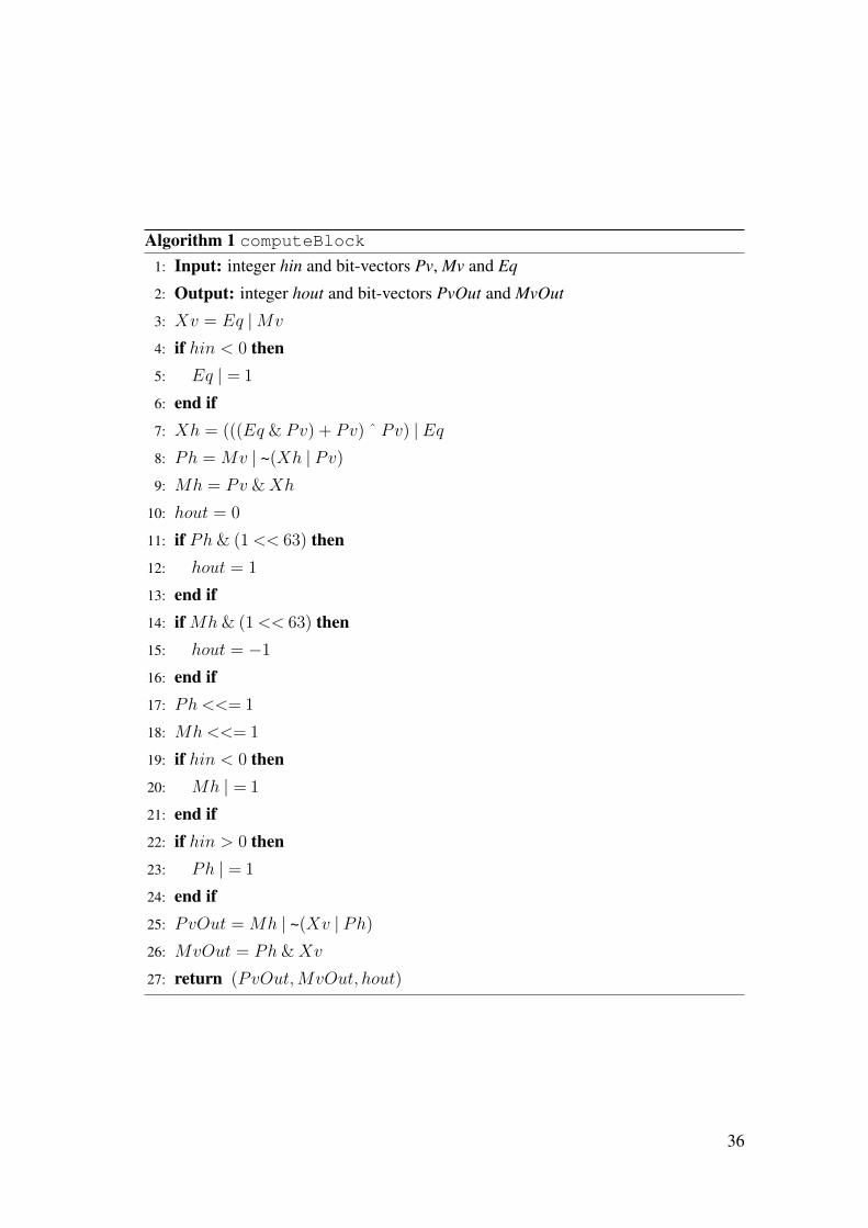
C-like pseudocode 1 shows how block computation is done in Myers. In EDLIB we
optimized this code by removing if statements and substituting them with bitwise
operations. This way, we achieved speed up of about 30% - 40%. C-like pseudocode
2 is our optimized version of block computation.
4.2.4. Dynamic adjustment of k
Another optimization that we added in EDLIB is dynamic adjustment of k. In HW and
SHW alignment methods, we adjust k during computation by always updating it to
best solution that was found so far. This approach would not be good if we wanted to
find all solutions that are smaller than k, but since we are looking for the best solution
that is smaller than k we can use it. By adjusting k during computation we narrow the
band and therefore speed up the computation.
4.2.5. Working with undefined k
In EDLIB, k does not need to be defined. In such case, we assume that best solution is
wanted, however big it may be. We could easily set k to highest value supported by its
data type, but if we work with k that is not much bigger then the best solution, then the
computation performs much faster. Therefore, we want to guess such k and use it for
35
Algorithm 1 computeBlock1: Input: integer hin and bit-vectors Pv, Mv and Eq
2: Output: integer hout and bit-vectors PvOut and MvOut
3: Xv = Eq |Mv
4: if hin < 0 then5: Eq | = 1
6: end if7: Xh = (((Eq & Pv) + Pv) ˆ Pv) | Eq8: Ph = Mv | ~(Xh | Pv)
9: Mh = Pv &Xh
10: hout = 0
11: if Ph& (1<< 63) then12: hout = 1
13: end if14: if Mh& (1<< 63) then15: hout = −1
16: end if17: Ph <<= 1
18: Mh<<= 1
19: if hin < 0 then20: Mh | = 1
21: end if22: if hin > 0 then23: Ph | = 1
24: end if25: PvOut = Mh | ~(Xv | Ph)
26: MvOut = Ph&Xv
27: return (PvOut,MvOut, hout)
36

Algorithm 2 computeBlockOptimized1: Input: integer hin and bit-vectors Pv, Mv and Eq
2: Output: integer hout and bit-vectors PvOut and MvOut
3: hinIsNeg = (hin >> 2) & 1
4: Xv = Eq |Mv
5: Eq | = hinIsNeg
6: Xh = (((Eq & Pv) + Pv) ˆ Pv) | Eq7: Ph = Mv | ~(Xh | Pv)
8: Mh = Pv &Xh
9: hout = 0
10: hout = (Ph& (1<< 63))>> 63
11: hout− = (Mh& (1<< 63))>> 63
12: Ph <<= 1
13: Mh<<= 1
14: Mh | = hinIsNeg
15: Ph | = (hin+ 1)>> 1
16: PvOut = Mh | ~(Xv | Ph)
17: MvOut = Ph&Xv
18: return (PvOut,MvOut, hout)
37

computation.
We start computation with k = w (we tried with different start values and this gave the
best result). If computation does not return any result, then we multiply k by two and
repeat the computation. We repeat this process until solution is found.
4.3. Aligner
For each of libraries we also created basic aligner that serves as an example, for testing
and also as useful tool. Aligner is used through command line and can be given various
options.
Both aligners take fasta files for input and return best score. No alphabet needs to
be specified because aligners detect alphabet automatically, while reading query and
target. Alignment method can be specified as option to both aligners, if not specified
default method is used.
SWIMD aligner also takes some additional options like score matrix and gap penal-
ties. Aligner comes with few already prepared score matrices, but custom score matri-
ces can also be used.
EDLIB aligner takes following additional options: option to find and print align-
ment path, option to set parameter k, option to find scores for only N best sequences.
Besides best score EDLIB aligner also returns position in target where alignment ends.
38

5. Results and discussion
In this chapter we compare speed of our libraries with currently best sequence align-
ment implementations available. We measured execution time using C++ function
clock() from ctime library. All aligners were compiled using gcc with -O3 op-
tion. All times are in seconds.
5.1. SWIMD
In this section we describe results of speed comparison of SWIMD with three other
aligners: SSWL [11], SSEARCH(FASTA) [17] and SWIPE [6]. We chose this three
aligners because they are currently best available. SSWL, SSEARCH and SWIPE do
only local alignment so we compared only for local alignment method. SSEARCH is
based on Fararr’s Striped SW [7]. SSWL is both library and aligner, while SSEARCH
and SWIPE are only aligners.
Aligners were tested by querying protein sequences against Swiss-Prot protein
database (contains 541762 sequences, total of 192577305 residues).
Following sequences were used: O74807 (110 residues), P19930 (195 residues), Q3ZAI3
(390 residues), P18080 (513 residues). All sequences and database were obtained from
UniProt (http://www.uniprot.org).
All tests were performed on only one thread, and only scores were calculated (not
alignments). Time spent to read query sequences and database was not measured.
Aligners were tested with following parameters:
– gap opening = 3
– gap extension = 1
– score matrix = BLOSUM50
Aligners were called using following commands:
– SSWL: ./ssw_test -p uniprot_sprot.fasta <query_file>
– SWIMD: ./swimd_aligner -s <query_file> uniprot_sprot.fasta
39

– SSEARCH: ./ssearch36 -d 0 -T 1 -p -f -3 -g -1 -s BL50
<query_file> uniprot_sprot.fasta
– SWIPE: ./swipe -a 1 -p 1 -G 3 -E 1 -M BLOSUM50 -b 0 -i
<query_file> -d uniprot_sprot
Database for SWIPE had to be preprocessed using program makeblastdb.
Chart 5.1 shows how much time took for different sequences to be aligned against
UniProtKB/Swiss-Prot database. Tests were performed on Intel Core i7-4770K CPU
@ 3.50GHz with 32GB RAM (AVX2 support). SWIMD was tested both using SSE4.1
and using AVX2.
Figure 5.1: Chart comparing SWIMD with SSWL, SSEARCH and SWIPE.
As we expected, SWIMD with AVX2 was two times faster than SWIMD with
SSE4.1 and was the fastest aligner.
Interesting result is that SWIPE is faster than SWIMD with SSE4.1 although we based
SWIMD on SWIPE. We believe that reason for this is that SWIMD code is not opti-
mized enough. Since we were writing SWIMD for multiple alignment methods and
for AVX2, we gave more care to keeping the code reusable then to optimizing details.
Some optimizations that could be done is doing check for sequence end on each fourth
40

column, processing few columns at once in order to optimaly use cache and replacing
intrinsics with assembly code.
5.2. EDLIB
In this section we describe results of comparison of EDLIB with SSWL, with Myers’s
implementation and with Landau Vishkin [3] implementation from SNAP [2].
Tests were performed on Intel Core i3 M 350 @ 2.27GHz with 4GB RAM.
5.2.1. Comparison with SSWL
To compare SSWL with EDLIB, we used two different scenarios: genome read align-
ment and protein comparison. Since we can not specify argument k to SSWL, we also
did not specify it to EDLIB.
Genome read alignment
We compared how fast can aligners align reads to genome. Alignment method from
EDLIB best suited for this purpose is HW, so we compared EDLIB using HW with
SSWL using local alignment.
We used two genome sequences available from National Center for Biotechnology
Information (NCBI):
– e_coli_536 (ftp://ftp.ncbi.nlm.nih.gov/genomes/Bacteria/
Escherichia_coli_536_uid58531/NC_008253.fna)
– e_coli_DH1 (ftp://ftp.ncbi.nlm.nih.gov/genomes/Bacteria/
Escherichia_coli_DH1_uid161951/NC_017625.fna)
For generating reads we used Illumina read simulator Mason [18], available on (http:
//www.seqan.de/projects/mason/).
To generate N reads of length n from e_coli_DH1 we used command ./mason
illumina -N <N> -n <n> -o reads.fasta e_coli_DH1.fasta. In our
tests, we aligned reads from e_coli_DH1 to e_coli_536.
We executed aligners using following commands:
– EDLIB: ./aligner -a HW reads.fasta e_coli_536.fasta
– SSWL: ./ssw_test e_coli_536.fasta reads.fasta
Table 5.1 shows performance of EDLIB and SSWL for different lengths of reads.
41

N = 10, n = 1000 N = 100, n = 100 N = 200, n = 50
EDLIB 12.3 12.8 16.8
SSWL 21.0 49.0 80.0
Table 5.1: Comparison of EDLIB with SSWL for aligning genome reads. Time is in seconds.
Finding alignment path Next, we compared speed of EDLIB and SSW for different
alignment methods with and without returning an alignment path.
For NW alignment method, we used prefix of length 100000 of e_coli_DH1 as
query and prefix of length 100000 of e_coli_536 as target. Table 5.2 shows results
of this comparison. SSWL was not able to return alignment path. It is important to
notice that EDLIB consumed large amount of memory for finding alignment path in
this example.
NW without align. path with align. path
EDLIB 0.98 3.9
SSWL 6.23 -
Table 5.2: Comparison of EDLIB (NW) with SSWL with and without returning alignment
path. Time is in seconds.
For HW alignment method, we used one Illumina read from e_coli_DH1 of length
1000 as query and e_coli_536 as target. Table 5.3 shows results of this comparison.
HW without align. path with align. path
EDLIB 0.15 0.16
SSWL 1.95 1.95
Table 5.3: Comparison of EDLIB (HW) with SSWL with and without returning alignment
path. Time is in seconds.
For SHW alignment method, we used prefix of length 10000 of e_coli_DH1 as
query and e_coli_536 as target. Table 5.4 shows results of this comparison.
42

SHW without align. path with align. path
EDLIB 0.02 0.04
SSWL 19.11 19.44
Table 5.4: Comparison of EDLIB (SHW) with SSWL with and without returning alignment
path. Time is in seconds.
EDLIB has shown to be faster then SSWL, especially for small reads. However, we
can see that EDLIB is somewhat slower for small reads than for large reads. Reason
for that is that block in EDLIB is of similar size to query(read) and therefore the is not
really any reducing of band, except when band stops to exist.
Results of finding alignment were as expected: for HW and small query EDLIB
was equally fast with and without finding alignment path. In example for SHW, finding
alignment path was somewhat slower compared to returning only score, but reason for
that is long query. Finding alignment path for NW was slower than returning only
score, which was expected. Important property of EDLIB is that for HW and SHW,
when query is much smaller than target, finding alignment does not affect time of
computation. This property is significant because in most cases, HW and SHW are run
on queries much smaller than target.
Protein comparison
We compared how fast can aligners compare two proteins. Alignment method from
EDLIB best suited for this purpose is NW, so we compared EDLIB using NW with
SSWL using local alignment. We tested for two different scenarios: for similar proteins
and for dissimilar proteins.
We generated proteins artificially, in random fashion. Similar proteins were created
by generating one of them randomly, and then changing it to get similar protein.
We executed aligners using following commands:
– EDLIB: ./aligner -a NW prot1.fasta prot2.fasta
– SSWL: ./ssw_test -p prot1.fasta prot2.fasta
Table 5.5 shows performance of EDLIB and SSWL for similar and dissimilar pro-
teins (~100000 in length each - there are no real proteins that long, but we used them
to get measurable times of computation).
43

similar dissimilar
EDLIB 0.01 1.56
SSWL 7.00 7.00
Table 5.5: Comparison of EDLIB with SSWL for comparing proteins. Time is in seconds.
For similar proteins EDLIB is much faster than SSWL, because of its banded algo-
rithm. For dissimilar proteins, EDLIB is still faster but not so much, since band is not
so narrow for dissimilar sequences.
5.2.2. Comparison with Myers’s implementation
We compared EDLIB with Myers’s implementation of his own banded block algorithm
from [12]. Since Myers’s implementation has only HW alignment method, we also
used HW for EDLIB.
In our tests we align read of length n from e_coli_DH1 with e_coli_536.
We executed aligners using following commands:
– EDLIB: ./aligner -a HW -k <k> -s read.fasta e_coli_536.fasta
– Myers: ./myers ‘cat read.fasta‘ <k> e_coli_536.fasta
Tables 5.6 shows performance of EDLIB and Myers’s implementation for different
lengths of read and different values of k.
n = 50 k = 0 k = 5 k = 10 k = 25 k = 50
EDLIB 0.061 0.101 0.100 0.097 0.93
Myers 0.069 0.066 0.065 0.114 0.100
n = 1000 k = 0 k = 10 k = 50 k = 100 k = 500
EDLIB 0.060 0.155 0.208 0.243 0.461
Myers 0.065 0.070 0.173 0.297 1.143
Table 5.6: Comparison of EDLIB with Myers’s implementation. Time is in seconds.
Results show that EDLIB and Myers’s implementation have similar speed, as was
expected since EDLIB is based on [12]. Sometimes it happens that Myers’s imple-
mentation is two times faster then EDLIB. We believe that reason for that is strong
reduction, which seems to be more effective in Myers’s implementation.
44

5.2.3. Comparison with Landau Vishkin
We compared EDLIB with Landau Vishkin implementation which we extracted from
SNAP. Since Landau Vishkin from SNAP supports only SHW, we compared only for
SHW method.
In our tests we aligned artificially generated proteins of different lengths and sim-
ilarity. For each pair of query and target we measured the time of running 10000
computations. Time for loading sequences was not measured. Results are shown in
table 5.7.
query length target length score k EDLIB LV
1000 10000 69 100 1.11 0.58
1000 10000 99 120 1.1 1.23
1000 10000 120 150 1.15 1.77
1000 10000 219 250 1.41 6.09
1000 10000 799 900 2.3 68.1
100 1000 19 30 0.12 0.04
100 1000 82 90 0.13 0.68
Table 5.7: Comparison of EDLIB with Landau Vishkin (SHW method). score is edit distance
between query and target. Time is in seconds.
Results show that Landau Vishkin is faster for small scores, while EDLIB is faster
for larger scores. This was expected, because Landau Vishkin algorithm is especially
efficient for small scores. From this results, we conclude that it could be beneficial
for EDLIB, when using SHW alignment method, to use Landau Vishkin algorithm for
small k, and after some threshold switch to Myers’s algorithm.
45

6. Conclusion
We implemented two fast C/C++ sequence alignment libraries, both of them based
on algorithms that use SIMD for parallelization. By extending existing algorithms
with additional features and making libraries easy to include and use, we made this
otherwise complex algorithms suitable for usage as components in bioinformatic and
other tools.
Table 6.1 shows main features of SWIMD and EDLIB, compared with features of
SWIPE and Myers.
Library SW NW HW SHW OV Align. path SSE AVX2
SWIMD Y Y Y Y N Y N Y Y
SWIPE N Y N N N N Y Y N
EDLIB Y N/A Y Y Y N/A Y N/A N/A
Myers N N/A N Y N N/A N N/A N/A
Table 6.1: Main features of EDLIB and SWIMD compared with SWIPE and Myers. Y is for
Yes, N is for No, and N/A is for Not Applicable.
For each library we implemented aligner which reads fasta sequences and also
provides additional options, depending on library.
We shortly explained local, global and few semi-global alignment methods and
compared their usage. For each of them we have shown scenario in which it is most
useful.
It is interesting to mention that in EDLIB we devised our own algorithm for ad-
justing the band of global alignment method. Another interesting modification that
we added is block computation optimization. By adding finding of alignment path
we made library usable in more applications, and have also shown how different align-
ment methods are appropriate in different situations and can be used together to achieve
wanted result.
46

Adding support for AVX2 in SWIMD worked as expected by providing two times
speed up, and comparing it with other algorithms we have shown that SWIMD with
AVX2 is the fastest database search algorithm.
SWIMD using SSE4.1 is somewhat slower than SWIPE, and EDLIB in some sit-
uations works slower than Myers’s implementation. Therefore, although a challenge
while trying to mantain reusable and extensible code, there is still space for improve-
ment and further optimization of both libraries.
We believe, since there is not many sequence alignment libraries available, that
libraries we implemented are going to be very useful and improve both performance
and development of many bioinformatics tools.
47

BIBLIOGRAPHY
[1] S. F. Altschul, W. Gish, W. Miller, E. W. Myers, and D. J. Lipman, “Basic local
alignment search tool,” Journal of molecular biology, vol. 215, no. 3, pp. 403–
410, 1990.
[2] M. Zaharia, W. J. Bolosky, K. Curtis, A. Fox, D. Patterson, S. Shenker, I. Stoica,
R. M. Karp, and T. Sittler, “Faster and more accurate sequence alignment with
snap,” arXiv preprint arXiv:1111.5572, 2011.
[3] G. M. Landau, U. Vishkin, and R. Nussinov, “An efficient string matching algo-
rithm with k differences for nudeotide and amino acid sequences,” Nucleic acids
research, vol. 14, no. 1, pp. 31–46, 1986.
[4] T. Smith, M. Waterman, and W. Fitch, “Comparative biosequence metrics,” Jour-
nal of Molecular Evolution, vol. 18, no. 1, pp. 38–46, 1981.
[5] O. Gotoh, “An improved algorithm for matching biological sequences,” Journal
of molecular biology, vol. 162, no. 3, pp. 705–708, 1982.
[6] T. Rognes, “Faster smith-waterman database searches with inter-sequence simd
parallelisation,” BMC bioinformatics, vol. 12, no. 1, p. 221, 2011.
[7] M. Farrar, “Striped smith–waterman speeds database searches six times over
other simd implementations,” Bioinformatics, vol. 23, no. 2, pp. 156–161, 2007.
[8] A. Szalkowski, C. Ledergerber, P. Krähenbühl, and C. Dessimoz, “Swps3–fast
multi-threaded vectorized smith-waterman for ibm cell/be and× 86/sse2,” BMC
Research Notes, vol. 1, no. 1, p. 107, 2008.
[9] M. Korpar and M. Šikic, “Sw#–gpu-enabled exact alignments on genome scale,”
Bioinformatics, p. btt410, 2013.
48

[10] Y. Liu, A. Wirawan, and B. Schmidt, “Cudasw++ 3.0: accelerating smith-
waterman protein database search by coupling cpu and gpu simd instructions,”
BMC bioinformatics, vol. 14, no. 1, p. 117, 2013.
[11] M. Zhao, W.-P. Lee, E. P. Garrison, and G. T. Marth, “Ssw library: An simd
smith-waterman c/c++ library for use in genomic applications,” PloS one, vol. 8,
no. 12, p. e82138, 2013.
[12] G. Myers, “A fast bit-vector algorithm for approximate string matching based on
dynamic programming,” Journal of the ACM (JACM), vol. 46, no. 3, pp. 395–415,
1999.
[13] “Intel SPMD Program Compiler.” https://ispc.github.io/. [Online;
accessed 22-June-2014].
[14] S. B. Needleman and C. D. Wunsch, “A general method applicable to the search
for similarities in the amino acid sequence of two proteins,” Journal of molecular
biology, vol. 48, no. 3, pp. 443–453, 1970.
[15] A. Wozniak, “Using video-oriented instructions to speed up sequence compari-
son,” Computer applications in the biosciences: CABIOS, vol. 13, no. 2, pp. 145–
150, 1997.
[16] E. Ukkonen, “Algorithms for approximate string matching,” Information and
control, vol. 64, no. 1, pp. 100–118, 1985.
[17] W. R. Pearson, “[5] rapid and sensitive sequence comparison with fastp and
fasta,” Methods in enzymology, vol. 183, pp. 63–98, 1990.
[18] M. Holtgrewe, “Mason–a read simulator for second generation sequencing data,”
Technical Report FU Berlin, 2010.
49

An SIMD dynamic programming C/C++ Library
Abstract
Deterministic sequence alignment algorithms like Smith-Waterman and Needleman-
Wunsch are slow but give optimal result. They are used in many bioinformatic tools as
core components and very often they consume significant amount of CPU time. In or-
der to make them faster, different fast implementations have been implemented, many
of them performing parallelization using Single Instruction Multiple Data (SIMD) sup-
port on CPU or GPU. However, most of these fast implementations are either stand-
alone tool or part of larger tool and were not made to be reusable, which is limiting
their usage.
In order to make some of this implementations reusable, we implemented two
C/C++ libraries for sequence alignment, both based on fast SIMD implementations.
SWIMD is library for database search and is based on Rognes’s Faster Smith-Waterman
database searches (SWIPE). In our implementation we added one global and two semi-
global alignment methods. We also added support for AVX2 instruction set. We com-
pared SWIMD with currently best implementations like SSW, SSEARCH and SWIPE
and showed that SWIMD implementation using AVX2 is the fastest.
SWIMD is available from http://github.com/Martinsos/swimd.
EDLIB is library for pairwise sequence alignment using edit distance and is based on
Myers’s Fast Bit-Vector Algorithm. We added one global and one semi-global align-
ment method. For global method we have shown how to calculate the band. We also
added finding of alignment path.
EDLIB is available from https://github.com/Martinsos/edlib.
By implementing this two libraries we provided reusable components important
for many bioinformatic tools, but also usable for other purposes. We believe this will
enable wider usage of fast SIMD algorithms and that many tools could benefit from
using them.
Keywords: bioinformatics, sequence, alignment, SIMD, SSE, AVX2, library, paral-
lelization
C/C++ biblioteka za dinamicko programiranje korištenjem SIMD instrukcija
Sažetak
Deterministicki algoritmi za poravnanje sekvenci poput Smith-Waterman algoritma
i Needleman-Wunsch algoritma su spori ali daju optimalno rješenje. Koriste se u
mnogim bioinformatickim alatima kao centralna komponenta i cesto veliki dio ukupnog
vremena racunanja odlazi upravo na njih. Kako bi se takvi algoritmi ubrzali nastale su
brojne brze implementacije, od kojih veliki dio provodi paralelizaciju korištenjem ista-
instrukcija-razliciti-podaci (engl. Single Instruction Multiple Data) (SIMD) podrške na
procesoru ili grafickoj kartici. Vecina takvih brzih implementacija su samostalni alat
ili dio nekog veceg alata te nisu napravljene za ponovno korištenje, što ogranicava
njihovu uporabu.
Kako bismo neke od brzih implementacija ucinili ponovno iskoristivima imple-
mentirali smo dvije C/C++ biblioteke za poravnanje sekvenci, obje temeljene na brzim
SIMD implementacijama.
SWIMD je biblioteka za pretragu baze i temelji se na Faster Smith-Waterman database
searches (SWIPE) od Rognes-a. U našoj implementaciji dodali smo jednu globalnu i
dvije polu-globalne metode poravnanja. Takoder smo dodali podršku za AVX2 skup
instrukcija. Usporedili smo SWIMD sa trenutno najboljim implementacijama: SSW,
SSEARCH i SWIPE. Pokazali smo da je SWIMD uz korištenje AVX2 skupa instruk-
cija najbrža implementacija.
SWIMD je dostupan na http://github.com/Martinsos/swimd.
EDLIB je biblioteka za poravnanje dvaju sekvenci koristeci udaljenost uredivanja i
temelji se na Fast Bit-Vector Algorithm od Myers-a. u EDLIB-u smo dodali jednu glob-
alnu i jednu polu-globalnu metodu poravnanja. Za globalnu metodu smo pokazali kako
izracunati pojas celija u matrici koje su dio rješenja. Takoder smo dodali pronalazak
puta poravnanja. EDLIB je dostupan na https://github.com/Martinsos/edlib.
Stvorivši SWIMD i EDLIB stvorili smo ponovno iskoristive komponente važne za
brojne bioinformaticke alate ali takoder iskoristive i u druge svrhe. Vjerujemo da ce
SWIMD i EDLIB omoguciti širu upotrebu brzih SIMD algoritama i da ce mnogi alati
imati koristi od njih.
Kljucne rijeci: bioinformatika, sekvenca, poravnanje, SIMD, SSE, AVX2, biblioteka,
paralelizacija