analysis and numerical approximation of brinkman ...€¦ · analysis and numerical approximation...

Analysis and Numerical approximation of

Brinkman regularization of two-phase flows

in porous media

G. Coclite and S. Mishra and N. Risebro and F. Weber

Research Report No. 2013-44November 2013

Seminar für Angewandte MathematikEidgenössische Technische Hochschule

CH-8092 ZürichSwitzerland

____________________________________________________________________________________________________

Funding ERC: 306279 SPARCCLE

ANALYSIS AND NUMERICAL APPROXIMATION OF

BRINKMAN REGULARIZATION OF TWO PHASE FLOWS

IN POROUS MEDIA

G. M. COCLITE, S. MISHRA, N. H. RISEBRO, AND F. R. WEBER

Abstract. We consider a hyperbolic-elliptic system of PDEs that arises in the modeling of

two-phase flows in a porous medium. The phase velocities are modeled using a Brinkmanregularization of the classical Darcy’s law. We propose a notion of weak solutions for these

equations and prove existence of these solutions. An efficient finite difference scheme is proposedand is shown to converge to the weak solutions of this system. The Darcy limit of the Brinkmanregularization is studied numerically using the convergent finite difference scheme in two spacedimensions as well as using both analytical and numerical tools in one space dimension.

1. The two Phase Flow Problem

Two phase flows in a porous medium model many interesting phenomena in geophysics.As examples, we mention water flooding of oil reservoirs and carbon dioxide sequestrationin subsurface formations.

A prototypical situation of interest is the flow of two phases, say oil and water in aporous medium. The variables of interest are the phase saturations sw and so representingthe saturation (volume fraction) of the water and oil phase respectively. We have theidentity:

(1.1) sw + so ≡ 1.

Hence, we can describe the dynamics in terms of the saturation of either of the two phases.We denote the water saturation as sw = s in the discussion below. Assuming a constantporosity (φ ≡ 1), the two phases are transported by [3]

(1.2) (sr)t + divx(vr) = 0, r ∈ w, o.Here, the phase velocities are denoted by vw and vo respectively. In view of the identity(1.1), the two phase velocities can be summed up to yield the incompressibility condition,

(1.3) divx(v) = 0, v = vw + vo.

The total velocity is denoted by v.The phase velocities in a homogeneous isotropic medium are described by the Darcy’s

law [3]:

(1.4) vr = −λr∇xpr, r ∈ w, o.The quantity λr = λr(sr) is the phase mobility and pr is the phase pressure. Note thatwe have neglected gravity in the above version of the Darcy’s law (gravity can be readilyconsidered, leading to an additional term, see [3]). Assume that the capillary pressure i.e,pc = pw − po is zero, we can sum (1.4) for both phases and obtain

(1.5) v = −λT (s)∇xp,

with p = pw = po being the pressure and λT = λw + λo being the total mobility.

Date: November 8, 2013.The work of SM was partially supported by ERC FP7 grant no. StG 306279 SPARCCLE.

1

2 G. M. COCLITE, S. MISHRA, N. H. RISEBRO, AND FRANZISKA WEBER

Using (1.5), the gradient of pressure in (1.4) can be eliminated leading to

(1.6) vw =λw(s)

λT (s)v.

Denoting the fractional flow function f as

(1.7) f(s) =λw(s)

λT (s)=

λw(s)

λw(s) + λo(s),

the saturation equation (1.2) for water can be written down as

(1.8) st + divx(f(s)v) = 0.

Combining the saturation equation with the incompressibility condition (1.3) and thepressure equation, we obtain the evolution equations for two phase flow in a porousmedium:

(1.9)

st + divx(f(s)v) = 0,

divx(v) = 0,

v = −λT (s)∇xp.

The above equations have to be augmented by suitable initial and boundary conditions.The phase mobility λw : [0, 1] 7→ R is a monotone increasing function with λw(0) = 0

and the phase mobility λo : [0, 1] 7→ R is a monotone decreasing function with λo(1) = 0.Furthermore, the total mobility is strictly positive i.e, λT ≥ λ∗ > 0 for some λ∗.

The above equations are a hyperbolic-elliptic system as the saturation equation in (1.9)is a scalar hyperbolic conservation law in several space dimensions with a coefficient givenby the velocity v. The velocity can be obtained by solving an elliptic equation for thepressure p.

It is well known that solutions of hyperbolic conservation laws can develop discontinu-ities, even for smooth initial data, [8]. The presence of these discontinuities or shock wavesimplies that solutions of conservation laws are sought in a weak sense and are augmentedwith additional admissibility criteria or entropy conditions in order to ensure uniqueness.

As the two phase flow equations involve a conservation law, we need to define a suitableconcept of entropy solutions for these equations and show that these solutions are well-posed. The problem of proving well-posedness of global weak solutions of the two phaseflow equations (1.9) has remained open for many decades. The main challenge in showingexistence is the fact that the velocity field v acts as a coefficient in the saturation equations.Although conservation laws with coefficients have been studied extensively in recent years,see [1, 13, 6, 2] and references therein, the state of the art results require that the coefficientis a function of bounded variation. Many attempts at showing that the velocity fieldv in (1.8) is sufficiently regular, for example is a BV function or has enough Sobolevregularity, have failed. Partial results (with strong assumptions on the velocity field oron the solution) have been obtained in [17, 20] and references therein.

Another approach is to consider a modified version of the two phase flow equations.Recalling that the two phase flow equations (1.9) were derived under the assumption thatthe capillary pressure was zero. Adding small but non-zero capillary pressure leads to aviscous perturbation of the saturation equation, see [14]. The viscous problem has beenshown to be well-posed in [14]. However, the fact that the coefficient of viscosity canbe very small leads to difficulties in numerical approximation of these equations as theviscous scales have to resolved. Furthermore, sharp saturation fronts might be smeareddue to the added viscosity.

BRINKMAN REGULARIZATION 3

A different approach to the above two considers the more fundamental question- isthe Darcy’s law (1.4) correct ? Many studies have focused on this question and havefound that the Darcy’s law maybe inadequate to explain the dynamics of fluid flow inporous media, even for a single phase [4]. It is plausible that the problems of showing wellposedness for the full two-phase flow model can be attributed to the modeling deficienciesof the Darcy’s law.

Several modifications of the Darcy’s law have been proposed, see [5]. Of particularinterest in this paper is the Brinkman modification [4]. It is well known that this modi-fication explains the dynamics of flow in porous media, better than the Darcy model inmany situations of interest, see [18, 15] and references therein. The Brinkman model forthe phase velocity of each phase is given by,

(1.10) − µ∆xvr + vr = −λr∇xpr, r ∈ w, o.Here, µ denotes a small scale parameter. Note that the Brinkman approximation adds asmoothing term to Darcy’s law.

Adding the phase velocity relations (1.10) for both phases w, o and neglecting capillarypressure i.e, pw = po = p, we obtain that the total velocity v = vw + vo satisfies,

−µ∆xv + v = −λT (s)∇xp,

Applying the divergence operator to both sides of the above equation and using incom-pressibility (1.3), we obtain the following elliptic equation for the pressure.

(1.11) − divx (λT (s)∇xp) = 0

Here, we have labeled the water saturation s = sw. Combining this equation with theconservation of mass for the water phase and with the Brinkman approximation (1.10)describing the velocity of the water phase and the fractional flow function defined in (1.7),we obtain the following complete system,

(1.12)

∂ts+ divx (vw) = 0,

−µ∆xvw + vw = −f(s)λT (s)∇xp

−divx (λT (s)∇xp) = 0,

that describes the flow of two phases in a porous medium, obeying the Brinkman’s law.The system (1.12) is henceforth termed as the Brinkman regularization of two phase flowsin a porous medium. We remark that the Darcy system (1.9) can be obtained from theBrinkman regularization (1.12) by setting µ = 0 and rewriting the water phase velocityin terms of the fractional flow function.

The rest of this paper is concerned with the analysis and numerical approximation ofthe Brinkman regularization (1.12). Our aims are three fold:

• To define a suitable notion of solutions to the Brinkman regularization (1.12) andto show that these solutions exist.

• To design an efficient numerical scheme to approximate the Brinkman regulariza-tion for two phase flows and to prove that this scheme converges when the meshis refined.

• To compare the solutions of the Brinkman regularization with those of the standardDarcy model for two phase flow (1.9) in order to ascertain whether the Brinkmanregularization is a suitable approximation of the Darcy’s law in the regime of twophase flows.

The rest of this paper provides answers to the above questions and is organized as follows:in Section 2, equivalent forms of the Brinkman regularization are stated, a suitable notionof solutions is defined and the main existence theorem is described. Section 3 deals with


the proof of existence of the Brinkman regularization. A convergent numerical scheme forapproximating (1.12) is presented in Section 4. Finally, we provide further comparisonsbetween the Darcy and Brinkman models (particularly in one space dimension) in Section5.

2. Statement of Problem

In this section, we will consider the following Darcy-Brinkman system (1.12) augmentedwith initial and boundary conditions,

(2.1)

∂ts+ divx (vw) = 0, t > 0, x ∈ Ω,

−µ∆xvw + vw = −f(s)λT (s)∇xp, t > 0, x ∈ Ω,

−divx (λT (s)∇xp) = 0, t > 0, x ∈ Ω,

∂νp(t,x) = π(t,x), t > 0, x ∈ ∂Ω,

vw(t,x) · ν(x) = h(t,x), t > 0, x ∈ ∂Ω,∫

Ω p(t,x)dx = 0, t > 0,

s(0,x) = s0(x), x ∈ Ω,

where

(H.1) Ω is an open connected subset of RN , N ≥ 1, with smooth boundary and ν is theunit outer normal;

(H.2) f is a smooth Lipschitz bounded function, 0 < µ ≤ 1 is a constants, and h, π :(0,∞)× ∂Ω → R are smooth bounded maps;

(H.3) λT is smooth Lipschitz bounded such that λT (·) ≥ λ∗ for some constant λ∗ > 0,and λT f

′ and λ′T /λT are bounded;

(H.4) the initial datum s0 ∈ H1(Ω).

Note that all the above assumptions are consistent with the definitions of the phasemobilities in the Darcy’s law.

Formally applying the Helmholtz operator −µ∆x + 1 to the first equation in (2.1) weobtain the third order problem

(2.2)

∂ts− µ∆x∂ts− divx (f(s)λT (s)∇xp) = 0, t > 0, x ∈ Ω,

−divx (λT (s)∇xp) = 0, t > 0, x ∈ Ω,

∂νp(t,x) = π(t,x), t > 0, x ∈ ∂Ω,∫

Ω p(t,x)dx = 0, t > 0,

µ∂ν∂ts+ f(s)λT (s)π = h, t > 0, x ∈ ∂Ω,

s(0,x) = s0(x), x ∈ Ω.

Since we can rewrite the first equation in the form

(2.3) ∂ts− divx (µ∇x∂ts+ f(s)λT (s)∇xp) = 0,

the boundary condition on ∂ν∂ts reads as the flux boundary condition on (2.3). Indeedthe flux in (2.3) is µ∇x∂ts+ f(s)λT (s)∇xp, multiplying by the unit outer normal ν andusing the fact that ∂νp = π we have

(µ∇x∂ts+ f(s)λT (s)∇xp) · ν

∣∣∂Ω

=(µ∂ν∂ts+ f(s)λT (s) ∂νp

︸︷︷︸

=π

)∣∣∂Ω

=µ∂ν∂ts+ f(s)λT (s)π.

(2.4)

On the other hand, comparing the first equations in (2.1) and (2.2) we get

(2.5) vw = µ∇x∂ts+ f(s)λT (s)∇xp


therefore, (2.4) and the boundary condition on vw give

(2.6) µ∂ν∂ts+ f(s)λT (s)π = h, (0,∞)× ∂Ω.

Next, we introduce the notion of weak solutions to the Brinkman system (2.1) below.

Definition 2.1. Let s, p : [0,∞) × Ω → R, vw : [0,∞) × Ω → RN be functions. We say

that (s, vw, p) is a solution of (2.1) if

(D.1) for every T > 0

s ∈ W 1,∞(0, T ;H1(Ω)), p ∈ L∞(0, T ;H1(Ω) ∩W 2,1(Ω)), vw ∈ L∞(0, T ;H2(Ω));

(D.2) for every test function ϕ ∈ C∞(RN+1) with compact support, the following identityis satisfied,∫ ∞

0

∫

Ω(s∂tϕ+ vw∇ϕ) dtdx−

∫ ∞

0

∫

∂Ωhϕdtdx+

∫

Ωs0(x)ϕ(0, x)dx = 0,

∫ ∞

0

∫

ΩλT (s)∇p · ∇ϕ−

∫ ∞

0

∫

∂Ωπϕdtdx = 0;

(D.3) for every test function Φ ∈ C∞(RN+1;RN ) with compact support contained in R,the following identity is satisfied,

µ

∫ ∞

0

∫

Ω∇vw · ∇Φdtdx+

∫ ∞

0

∫

Ωvw · Φdtdx+

∫ ∞

0

∫

Ωf(s)λT (s)∇p · Φdtdx = 0;

(D.4) for almost every t > 0∫

Ωp(t,x)dx = 0.

Due to regularity assumption (D.2) and the linearity of the Helmholtz operator 1−µ∆the solutions of (2.1) solve (2.2) and vice versa.

Our main result is the following existence theorem.

Theorem 2.1. Assume (H.1), (H.2), (H.3), and (H.4). Then, the initial boundaryvalue problem (2.1) has a solution (s, p, vw) in the sense of Definition 2.1.

We use the following recursive approximation of (2.1).We start defining

(2.7) s0(t,x) = s0(x), t > 0, x ∈ Ω.

The function p0 = p0(t, x) solves the elliptic problem with time depending Neumannboundary conditions

(2.8)

−divx (λT (s0)∇xp0) = 0, t > 0, x ∈ Ω,

∂νp0(t,x) = π(t,x), t > 0, x ∈ ∂Ω,∫

Ω p0(t,x)dx = 0, t > 0,

then we define vw,0 = vw,0(t,x) as the solution of the following elliptic problem with timedepending boundary conditions

(2.9)

−µ∆xvw,0 + vw,0 = −f(s0)λT (s0)∇xp, t > 0, x ∈ Ω,

vw,0(t,x) · ν(x) = h(t,x), t > 0, x ∈ ∂Ω.

The next step in the algorithm is to define s1 = s1(t,x) as follows

(2.10) s1(t,x) = s0(x)−∫ t

0divx (vw,0) (τ,x)dτ, t > 0, x ∈ Ω,


namely s1 solves the problem

(2.11)

∂ts1 + divx (vw,0) = 0, t > 0, x ∈ Ω,

s1(0,x) = s0(x), x ∈ Ω.

In general for every n ∈ N we have

(2.12)

∂tsn+1 + divx (vw,n) = 0, t > 0, x ∈ Ω,

−µ∆xvw,n + vw,n = −f(sn)λT (sn)∇xpn, t > 0, x ∈ Ω,

−divx (λT (sn)∇xpn) = 0, t > 0, x ∈ Ω,

∂νpn(t,x) = π(t,x), t > 0, x ∈ ∂Ω,

vw,n(t,x) · ν(x) = h(t,x), t > 0, x ∈ ∂Ω,∫

Ω pn(t,x)dx = 0, t > 0,

sn+1(0,x) = s0(x), x ∈ Ω.

The above iteration scheme would be shown to converge in order to prove the existencetheorem 2.1 in the next section.n

3. A Priori Estimates and Proof of Theorem 2.1

This section is devoted to the proof of Theorem 2.1. We begin with some a prioriestimates on the solution (sn+1, vw,n, pn) of (2.12).

Lemma 3.1 (H1 estimate on pn). Let n ∈ N. We have that

pn ∈ L∞(0, T ;H1(Ω)), T > 0.

In particular

(3.1) ‖pn(t, ·)‖H1(Ω) ≤ C1 ‖π(t, ·)‖L2(∂Ω) , t > 0,

for some positive constant C1 independent on µ and n.

Proof. From the third equation in (2.12), (H.3), and the boundary conditions on pn,

λ∗

∫

Ω|∇xpn|2dx ≤

∫

ΩλT (sn)|∇xpn|2dx

=−∫

Ωdivx (λT (sn)∇xpn)︸︷︷︸

=0

pdx+

∫

∂ΩλT (sn)pn ∂νpn

︸︷︷︸

=π

dσ

=

∫

∂ΩλT (sn)πpndσ ≤

‖λT ‖2L∞(R)

2α

∫

∂Ωπ2dσ +

α

2

∫

∂Ωp2ndσ,

where α > 0 is a constant that will be chosen later. The zero mean condition on pn andthe Sobolev embeddings give

λ∗

∫

Ω|∇xpn|2dx ≤

‖λT ‖2L∞(R)

2α

∫

∂Ωπ2dσ +

α

2

∫

∂Ωp2ndσ

≤‖λT ‖2L∞(R)

2α

∫

∂Ωπ2dσ +

αc

2

∫

Ω|∇xpn|2dx,

where c is the Sobolev embedding constant. Choosing α = λ∗/c we get∫

Ω|∇xpn|2dx ≤

c ‖λT ‖2L∞(R)

λ2∗

∫

∂Ωπ2dσ.

The claim follows from the zero mean condition on pn.


Lemma 3.2. Let n ∈ N. We have that

vw,n ∈ L∞(0, T ;H2(Ω)),

for every T > 0. In particular

(3.2) ‖vw,n(t, ·)‖H2(Ω) ≤C3

µ

(

‖fλT ‖L∞(R) ‖π(t, ·)‖L2(∂Ω) + ‖h(t, ·)‖L2(∂Ω)

)

,

for each t > 0 and some positive constant C3 independent on µ and n.

Proof. The claim follows directly from classical regularity results on elliptic equations andLemma 3.1.


sn ∈ W 1,∞(0, T ;H1(Ω)),

for every T > 0. In particular

‖sn(t, ·)‖H1(Ω) ≤ ‖s0‖H1(Ω) +C4

µ

(

‖fλT ‖L∞(R) ‖π(t, ·)‖L2(∂Ω) + ‖h(t, ·)‖L2(∂Ω)

)

,

‖∂tsn(t, ·)‖H1(Ω) ≤C4

µ

(

‖fλT ‖L∞(R) ‖π(t, ·)‖L2(∂Ω) + ‖h(t, ·)‖L2(∂Ω)

)

,

(3.3)

for each t > 0 and some positive constant C4 independent on µ and n.

Proof. The claim follows directly from the first equation in (2.12) and Lemma 3.2. Indeed,we have

s0(t,x) = s0(x),

sn+1(t,x) = s0(x)−∫ t

0divx (vw,n) (τ,x)dτ,

∂tsn+1 = −divx (vw,n) .


∆xpn ∈ L∞(0, T ;L1(Ω)), T > 0.

In particular

(3.4) ‖∆xpn(t, ·)‖L1(Ω) ≤ C5

(

‖π(t, ·)‖2L2(∂Ω) + ‖h(t, ·)‖2L2(∂Ω)

)

,

for each t > 0, where C5 is a positive constant independent on µ and n.

Proof. From (2.12)

∆xpn = −λ′T (sn)

λT (sn)∇xpn · ∇xsn,

therefore, thanks to (H.2) and (H.3),

‖∆xpn(t, ·)‖L1(Ω) ≤1

2

∥∥∥∥

λ′T

λT

∥∥∥∥L∞(R)

(

‖∇xpn(t, ·)‖2L2(Ω) + ‖∇xsn(t, ·)‖2L2(Ω)

)

.

The claim follows from Lemmas 3.1 and 3.3.


Proof of Theorem 2.1. Thanks to Lemmas 3.1, 3.2, 3.3, there exist three functions

(3.5) s, p : (0,∞)× Ω −→ R, vw : (0,∞)× Ω −→ RN ,

such that, for every T > 0,

s ∈ W 1,∞(0, T ;H1(Ω)), p ∈ L∞(0, T ;H1(Ω)), vw ∈ L∞(0, T ;H2(Ω)),

and, passing to a subsequence,

sn s, weakly in W 1,ℓ(0, T ;H1(Ω)), 1 ≤ ℓ < ∞, T > 0,

pn p, weakly in Lℓ(0, T ;H1(Ω)), 1 ≤ ℓ < ∞, T > 0,

vw,n vw, weakly in Lℓ(0, T ;H2(Ω)), 1 ≤ ℓ < ∞, T > 0.

(3.6)

In particular, we have that

sn → s, strongly in L2((0, T )× Ω), T > 0,

sn → s, a.e. in (0,∞)× Ω,

∇pn ∇p, weakly in L2((0, T )× Ω), T > 0.

(3.7)

Therefore, the distributional formulation of (2.12), the Dominated Convergence Theoremand the boundedness of f and λT implies (D.2), (D.3), and (D.4).

We conclude by proving that (D.1) holds. Thanks to (3.5) we have only to prove that

(3.8) p ∈ L∞(0, T ;W 2,1(Ω)).

Clearly, (3.6), Lemmas 3.1, 3.2, 3.3 and the weak lower semicontinuity if the norms givethe following estimates

‖p(t, ·)‖H1(Ω) ≤ C1 ‖π(t, ·)‖L2(∂Ω) ,

‖vw(t, ·)‖H2(Ω) ≤C3

µ

(

‖fλT ‖L∞(R) ‖π(t, ·)‖L2(∂Ω) + ‖h(t, ·)‖L2(∂Ω)

)

,

‖s(t, ·)‖H1(Ω) ≤ ‖s0‖H1(Ω) +C4

µ

(

‖fλT ‖L∞(R) ‖π(t, ·)‖L2(∂Ω) + ‖h(t, ·)‖L2(∂Ω)

)

,

‖∂ts(t, ·)‖H1(Ω) ≤C4

µ

(

‖fλT ‖L∞(R) ‖π(t, ·)‖L2(∂Ω) + ‖h(t, ·)‖L2(∂Ω)

)

,

for almost every t > 0.Since, from (2.1)

∆xp = −λ′T (s)

λT (s)∇xp · ∇xs,

therefore, thanks to (H.2) and (H.3),

‖∆xp(t, ·)‖L1(Ω) ≤1

2

∥∥∥∥

λ′T

λT

∥∥∥∥L∞(R)

(

‖∇xp(t, ·)‖2L2(Ω) + ‖∇xs(t, ·)‖2L2(Ω)

)

,

that proves (3.8).

Thus, we have shown that weak solutions of the Brinkman regularization of two-phaseflows in a porous medium (1.12) exist. The question of uniqueness is still open.

Remark 3.1. It must be emphasized that many of the estimates derived in the proof ofthe existence theorem 2.1 are µ dependent and blow up as the regularization parameterµ → 0. In particular, the estimate (3.2) on the phase velocity is µ-dependent as are theestimates on the saturation (3.3). Thus, in the limit µ → 0, which corresponds to theclassical Darcy’s law, we do not expect that the velocity field and the saturation are asregular as in the case of the Brinkman approximation. As an example, it is well known


that the saturation contains discontinuities in the form of shocks for the classical two-phaseflow problem which is inconsistent with the H1 estimate in (3.3). Hence, we have beenunable to obtain any convergence results for the Brinkman system (1.12) to the classicaltwo-phase Darcy system (1.9) as µ → 0.

Remark 3.2. Here, we have focused on the case of two-phase flows. A Brinkman regular-ization of multi phase flows can be obtained analogously to the derivation of the Brinkmantwo phase flow model in the introduction. This system for m (m ≥ 3) phases reads as

(3.9)

∂ts1 + divx (vw,1) = 0, t > 0, x ∈ Ω,

......

∂tsm + divx (vw,m) = 0, t > 0, x ∈ Ω,

−µ∆xvw,1 + vw,1 = −λ1(s1)∇xp, t > 0, x ∈ Ω,

......

−µ∆xvw,m + vw,m = −λm(sm)∇xp, t > 0, x ∈ Ω,

−divx (λT (s1, .., sm)∇xp) = 0, t > 0, x ∈ Ω,

augmented with suitable initial and boundary conditions. As in definition 2.1, we cananalogously define a suitable notion of weak solutions and prove existence of solutionsby following the approximation procedure presented in section 2 and proving analogousestimates like those in the proof of theorem 2.1.

4. A convergent numerical scheme for the Brinkman regularization

In this section, we will present an efficient numerical scheme to approximate theBrinkman regularization for two-phase flow (1.12). For simplicity, we consider the unitsquare in two space dimensions i.e, Ω = [0, 1]2 ⊂ R

2. As many interesting benchmarktests include a source in the pressure equation (to model injection of water), we considerthe following modification of the Brinkman regularization (1.12),

(4.1)

∂ts+ divx (vw) = 0, t > 0, x ∈ Ω,

−µ∆xvw + vw = −f(s)λT (s)∇xp, t > 0, x ∈ Ω,

−divx (λT (s)∇xp) = q, t > 0, x ∈ Ω,

∂νp(t,x) = π(t,x), t > 0, x ∈ ∂Ω,

vw(t,x) · ν(x) = h(t,x), t > 0, x ∈ ∂Ω,∫

Ω p(t,x)dx = 0, t > 0,

s(0,x) = s0(x), x ∈ Ω,

Here, q ∈ L∞(0, T ;L2(Ω)) denotes a source function. Note that the existence resultTheorem 2.1 can be readily extended to this case of including a source term.

For the sake of definiteness, let vw = (u, v). The boundary values are π(t,x) = 0, and

(4.2)u(0, y) = u(1, y) = 0, ∂yu(x, 0) = ∂yu(x, 1) = 0

v(x, 0) = v(x, 1) = 0, ∂xv(0, y) = ∂xv(1, y) = 0.

We discretize the computational domain [0, 1]2 with on a Cartesian mesh with grid-points xi = (i − 1/2)∆x, yj = (j − 1/2)∆x, j = 1, . . . , N , ∆x = 1/N . Let pnij , v

nij , and

snij denote the approximation to p, vw and s respectively, evaluated at (xi, yj , tn), wheretn = n∆t. The scheme for pnij reads

(4.3) −Dx+

(

tni−1/2,jDx−p

nij

)

−Dy+

(

tni,j−1/2Dy−p

nij

)

= qnij , i, j = 1, . . . , N,


where

tni+1/2,j =λT (s

nij) + λT (s

ni+1,j)

2and tni,j+1/2 =

λT (snij) + λT (s

ni,j+1)

2,

with the boundary values

tn1/2,j = tnN+1/2,j = tni,1/2 = tni,N+1/2 = 0, for i, j = 1, . . . , N , n ≥ 0,

and

qnij = q(xi, yj), i, j = 1, . . . , N, n ≥ 0.

To define the scheme for vnij , we first define

fni+1/2,j =

f(snij) + f(sni+1,j)

2and fn

i,j+1/2 =f(snij) + f(sni,j+1)

2.

Then the scheme for uni+1/2,j reads

(4.4) − µ(Dx

+Dx− +Dy

+Dy−

)uni+1/2,j + uni+1/2,j = fn

i+1/2,jtni+1/2,jD

x+p

nij ,

for i = 1, . . . , N − 1, j = 1, . . . , N with boundary values

un1/2,j = unN+1/2,j = 0, j = 1, . . . , N.

Similarly, the scheme for vni,j+1/2 reads

(4.5) − µ(Dx

+Dx− +Dy

+Dy−

)vni,j+1/2 + vni,j+1/2 = fn

i,j+1/2tni,j+1/2D

y+p

nij ,

for i = 1, . . . , N , j = 1, . . . , N − 1 with boundary values

vni,1/2 = vni,N+1/2 = 0, i = 1, . . . , N.

Finally we update snij by

(4.6) sn+1ij =

1

4

(sni+1,j + sni−1,j + sni,j+1 + sni,j−1

)−∆t

(

Dx−u

ni+1/2,j +Dy

−vni,j+1/2

)

,

for n ≥ 0 and i, j = 1, . . . , N , with the initial values s0ij = s0(xi, yj).

4.1. Convergence of the scheme in 2D. We will show that the approximate solutionsgenerated by the finite difference scheme (4.3) – (4.6) converge to a weak solution of (4.1)for a fixed µ. To do so, we mimic the estimates of Lemmas 3.1 – 3.3 in the discrete setting.

From the discrete values snij , i, j = 0, . . . , N , n ≥ 0, we define the piecewise linearinterpolant

sn(x, y) = snij + (x− xi)Dx+s

nij + (y − yj)D

y+s

nij + (x− xi) (y − yj)D

y+D

x+s

nij

s∆(t;x, y) = sn(x, y) + (t− tn)Dt+s

n(x, y)

(t;x, y) ∈ [tn, tn+1)× [xi, xi+1)× [yj , yj+1), n ≥ 0, i, j = 0, . . . , N,

where we have denoted

Dt+s

n(x, y) =1

∆t(sn+1(x, y)− sn(x, y)),

the forward divided difference in the temporal direction. In a similar way, we definepn(x, y) to be the bilinear interpolation with pn(xi, yj) = pnij ; u

n(x, y) and vn(x, y) to be

the piecewise quadratic splines with un(xi+1/2, yj) = uni+1/2,j and vn(xi, yj+1/2) = vni,j+1/2,

and p∆(t;x, y), u∆(t;x, y) and v∆(t;x, y) to be the linear interpolations of pn(x, y), un(x, y)

and vn(x, y) in t between tn and tn+1, n ≥ 0.Now, we will show the following estimates on the approximate solutions:


Lemma 4.1. Let ∆ = (∆x,∆y,∆t), ∆x,∆y,∆t > 0 and q ∈ L∞(0, T ;L2(Ω)). We havep∆ ∈ L∞(0, T ;H1(Ω)) for any T > 0 with

(4.7) ‖p∆(t; ·)‖H1(Ω) ≤√2

λ∗‖q(t; ·)‖L2(Ω), 0 ≤ t ≤ T.

Proof. Using the identities∑

i,j

tni−1/2,j |Dx−p

nij |2 = −

∑

i,j

Dx+(t

ni−1/2,jD

x−p

nij) p

nij ,

∑

i,j

tni,j−1/2|Dy−p

nij |2 = −

∑

i,j

Dy+(t

ni,j−1/2D

y−p

nij) p

nij ,

multiplying (4.3) by pij and summing over the indices i, j, we obtain∑

i,j

(tni−1/2,j |Dx

−pnij |2 + tni,j−1/2|D

y−p

nij |2

)=

∑

i,j

qnijpnij .

Since tni−1/2,j , tni,j−1/2 ≥ λ∗ by assumption (H.3), and (αa2 + b2/α)/2 ≥ ab for a, b ∈ R,

α > 0, this yields∑

i,j

(|Dx

−pnij |2 + |Dy

−pnij |2

)≤ 1

2λ∗

(

α∑

i,j

(pnij)2 +

1

α

∑

i,j

(qnij)2

)

,

and hence

‖∂xp∆(t; ·)‖2L2(Ω) + ‖∂yp∆(t; ·)‖2L2(Ω) ≤1

2λ∗

(

α‖p∆(t; ·)‖2L2(Ω) +1

α‖q(t; ·)‖2L2(Ω)

)

Using Poincare’s inequality,

‖∇xf‖L2(Ω) ≤ C(Ω)‖f‖L2(Ω),

where for Ω = [0, 1]2, C(Ω) = 1, we obtain by choosing α = λ∗,

‖p∆(t; ·)‖L2(Ω), ‖∇xp∆(t; ·)‖L2(Ω) ≤1

λ∗‖q(t; ·)‖L2(Ω),

which implies (4.8).

Lemma 4.2. Let ∆ = (∆x,∆y,∆t), ∆x,∆y,∆t > 0, µ > 0 and q ∈ L∞(0, T ;L2(Ω)).Assume furthermore that fλT is bounded. Then u∆, v∆ ∈ L∞(0, T ;H2(Ω)) for T > 0with

µ2‖∇2xu∆(t; ·)‖2L2(Ω) + µ‖∇xu∆(t; ·)‖2L2(Ω) + ‖u∆(t; ·)‖2L2(Ω) ≤ C ‖fλT ‖2L∞‖∂xp∆(t; ·)‖2L2(Ω)

(4.8a)

µ2‖∇2xv∆(t; ·)‖2L2(Ω) + µ‖∇xv∆(t; ·)‖2L2(Ω) + ‖v∆(t; ·)‖2L2(Ω) ≤ C ‖fλT ‖2L∞‖∂yp∆(t; ·)‖2L2(Ω),

(4.8b)

where C > 0 is a scaling factor, not depending on the other quantities.

Proof. We take the square of equation (4.4), sum it over the indices i and j and use thesummation by parts identity

∑

i,j

uni+1/2,j(Dx+D

x− +Dy

+Dy−)u

ni+1/2,j = −

∑

i,j

(|Dx

−uni+1/2,j |2 + |Dy

−uni+1/2,j |2

)

to obtain

(4.9)∑

i,j

(|(Dx

+Dx− +Dy

+Dy−)u

ni+1/2,j |2 + 2µ(|Dx

−uni+1/2,j |2 + |Dy

−uni+1/2,j |2) + |uni+1/2,j |2

)


=∑

i,j

(fni+1/2,j)

2(tni+1/2,j)2|Dx

+pnij |2.

Using summation by parts twice for the first term on the right hand side of (4.9) gives∑

i,j

|(Dx+D

x− +Dy

+Dy−)u

ni+1/2,j |2

=∑

i,j

(|Dx

+Dx−u

ni+1/2,j |2 + |Dy

+Dy−u

ni+1/2,j |2 + 2|Dx

−Dy−u

ni+1/2,j |2

),

which implies (4.8a). In the same way, we can show (4.8b). Since p∆ ∈ L∞(0, T ;H1(Ω))by Lemma 4.1, we get u∆, v∆ ∈ L∞(0, T ;H2(Ω)).

Now it is easy to show that s∆ ∈ W 1,∞(0, T ;L2(Ω)) ∩ L∞(0, T ;H1(Ω)):

Lemma 4.3. Let ∆ = (∆x,∆y,∆t), ∆x,∆y,∆t > 0 with ∆x/∆t,∆y/∆t ≤ K, where0 < K < ∞, and let µ > 0. Moreover assume q ∈ L∞(0, T ;L2(Ω)), s0 ∈ H1(Ω) and thatfλT is bounded. Then s∆ ∈ W 1,∞(0, T ;L2(Ω)) ∩ L∞(0, T ;H1(Ω)) for T > 0 with

‖s∆(t; ·)‖L2(Ω) ≤ ‖s0‖L2(Ω) +C t

λ∗√µ‖fλT ‖L∞‖q‖L∞(0,T ;L2(Ω)),(4.10a)

‖∇xs∆(t; ·)‖L2(Ω) ≤ ‖∇xs0‖L2(Ω) +C t

λ∗µ‖fλT ‖L∞‖q‖L∞(0,T ;L2(Ω)),

(4.10b)

‖∂ts∆(t; ·)‖L2(Ω) ≤ C(√K + 1)

(

‖∇xs0‖L2(Ω) +t

λ∗µ‖fλT ‖L∞‖q‖L∞(0,T ;L2(Ω))

)

,(4.10c)

for 0 ≤ t ≤ T and where C > 0 is a constant.

Proof. We take the square of equation (4.6), sum over the indices i, j and use triangleinequality to obtain

(∑

i,j

|sn+1ij |2

)1/2

≤(∑

i,j

|snij |2)1/2

+∆t

(∑

i,j

|Dx−u

ni+1/2,j +Dy

−uni,j+1/2|2

)1/2

,

which implies

‖sn+1‖L2(Ω) ≤ ‖sn‖L2(Ω) +∆t(‖∂xu∆(tn; ·)‖L2(Ω) + ‖∂yv∆(tn; ·)‖L2(Ω)

).

Iterating over n, this yields

‖sn‖L2(Ω) ≤ ‖s0‖L2(Ω) + tn(‖∇xu∆‖L∞(0,T ;L2(Ω)) + ‖∇xv∆‖L∞(0,T ;L2(Ω))

).

Using Lemma 4.1, we obtain

‖s∆(t; ·)‖L2(Ω) ≤ ‖s0‖L2(Ω) +C t√µ‖fλT ‖L∞‖∇xp‖L∞(0,T ;L2(Ω))

≤ ‖s0‖L2(Ω) +C t

λ∗√µ‖fλT ‖L∞‖q‖L∞(0,T ;L2(Ω)),

where we have used (4.8) for the second inequality. In order to show that the gradient ofs∆(t; ·) is in L2(Ω), we apply the linear operators Dx

+, Dy+ to the evolution equation for

snij , (4.6),

Dx+s

n+1ij =

1

4

(Dx

+sni+1,j +Dx

+sni−1,j +Dx

+sni,j+1 +Dx

+sni,j−1

)

−∆t(

Dx+D

x−u

ni+1/2,j +Dx

+Dy−v

ni,j+1/2

)

,


(and similarly for Dy+), then take the square of the above equation, sum over the indices

i, j and use again triangle inequality, to obtain(∑

i,j

|Dx+s

n+1ij |2

)1/2

≤(∑

i,j

|Dx+s

nij |2

)1/2

+∆t

(∑

i,j

|Dx+D

x−u

ni+1/2,j+Dx

+Dy−u

ni,j+1/2|2

)1/2

,

which implies after iteration over n,

‖∂xsn‖L2(Ω) ≤ ‖∂xs0‖L2(Ω) + tn(‖∂2

xu∆‖L∞(0,T ;L2(Ω)) + ‖∂x∂yv∆‖L∞(0,T ;L2(Ω))

).

Hence, using Lemmas 4.1 and 4.2, we obtain

‖∂xs∆(t; ·)‖L2(Ω) ≤ ‖∂xs0‖L2(Ω) +C t

λ∗µ‖fλT ‖L∞‖q‖L∞(0,T ;L2(Ω)).

In a similar way, we obtain an estimate for ‖∂ys∆(t; ·)‖L2(Ω) and thus

‖∇xs∆(t; ·)‖L2(Ω) ≤ ‖∇xs0‖L2(Ω) +C t

λ∗µ‖fλT ‖L∞‖q‖L∞(0,T ;L2(Ω)).

To obtain an estimate on ∂ts∆, we rewrite the evolution equation for snij as

(4.11)sn+1ij − snij

∆t=

1

4∆t

(∆x2Dx

+Dx−s

nij +∆y2Dy

+Dy−s

nij

)−(

Dx−u

ni+1/2,j +Dy

−vni,j+1/2

)

,

We notice that

∆x|Dx+D

x−s

nij | ≤ |Dx

+snij |+ |Dx

−snij |,

∆y|Dy+D

y−s

nij | ≤ |Dy

+snij |+ |Dy

−snij |,

which implies after taking the square of equation (4.11) and summing over i, j∑

i,j

|Dt+s

nij |2 ≤ K

∑

i,j

(|Dx

+snij |2 + |Dy

+snij |2

)+ 2

∑

i,j

(|Dx

−uni+1/2,j +Dy

−uni,j+1/2|2

).

Thus

‖∂ts∆(t; ·)‖L2(Ω) ≤ C(√

K‖∇xs∆‖L∞(0,T ;L2(Ω)) + ‖∂xu∆‖L∞(0,T ;L2(Ω)) + ‖∂yv∆‖L∞(0,T ;L2(Ω))

)

≤ C(√

K‖∇xs0‖L2(Ω) +(√K + 1)t

λ∗µ‖fλT ‖L∞‖q‖L∞(0,T ;L2(Ω))

)

,

where we have used (4.10b) and Lemmas 4.1 and 4.2 for the second inequality.

Now we are ready to prove the main convergence theorem for the finite differencescheme,

Theorem 4.1. Fix µ > 0 and assume q ∈ L∞(0, T ;L2(Ω)), s0 ∈ H1(Ω) and f, λT ∈L∞(R). Furthermore, let ∆ = (∆x,∆y,∆t) > 0 such that ∆x/∆t,∆y/∆t ≤ K < ∞.Then a subsequence of p∆∆>0, u∆∆>0, v∆∆>0, s∆∆>0, converges to a weak so-lution (p,vw, s) of (4.1) as ∆ → 0, and

s ∈ W 1,∞(0, T ;L2(Ω))∩L∞(0, T ;H1(Ω)), p ∈ L∞(0, T ;H1(Ω)), vw ∈ L∞(0, T ;H2(Ω)).

Proof. Due to the Lemmas 4.1, 4.2 and 4.3, we have for a subsequence

s∆ s, weakly in Lℓ(0, T ;H1(Ω)), 1 ≤ ℓ < ∞, T > 0,

p∆ p, weakly in Lℓ(0, T ;H1(Ω)), 1 ≤ ℓ < ∞, T > 0,

(u∆, v∆) vw, weakly in Lℓ(0, T ;H2(Ω)), 1 ≤ ℓ < ∞, T > 0.

(4.12)


The Aubin-Lions Lemma gives us the compact embeddingW 1,∞(0, T ;L2(Ω))∩L∞(0, T ;H1(Ω)) ⊂⊂ Lℓ(0, T ;L2(Ω)) for 1 ≤ ℓ < ∞, and hence

s∆ → s, strongly in L2((0, T )× Ω), T > 0, and

s∆ → s, a.e. in (0, T )× Ω,(4.13)

for a subsequence. We denote

Λn(s∆) =

(λnx 00 λn

y

)

, Fn(s∆) =

(fnx 00 fn

y

)

,

where λnx(s∆), λ

ny (s∆) are piecewise linear interpolations of tni+1/2,j and tni,j+1/2 satis-

fying λnx((s

nij + sni+1,j)/2) = tni+1/2,j and λn

x((snij + sni,j+1)/2) = tni,j+1/2 and similarly

fnx (s∆), f

ny (s∆) are piecewise linear interpolations of f

ni+1/2,j and fn

i,j+1/2 satisfying fnx ((s

nij+

sni+1,j)/2) = fni+1/2,j and fn

x ((snij + sni,j+1)/2) = fn

i,j+1/2. Then we let

Λ∆(s∆, t) = Λn(s∆), F∆(s∆, t) = Fn(s∆), t ∈ [tn, tn + 1), n ≥ 0.

Than, thanks to (4.13),

Λ∆(s∆, t) → λT (s), a.e. in (0, T )× Ω, and

F∆(s∆, t) → f(s), a.e. in (0, T )× Ω.(4.14)

Thus, using in addition, that

∇xp∆ ∇xp, weakly in L2((0, T )× Ω), T > 0,

the boundedness of f and λT , and the Dominated Convergence Theorem, we can pass tothe limit ∆ → 0 in the weak formulations

∫ T

0

∫

Ω

(

s∆∂tϕ+ (u∆, v∆)T∇xϕ− s∆

(∆x2

∆t∂2xϕ+

∆y2

∆t∂2yϕ

))

dx dt

+

∫

Ωs0(x)ϕ(0, x) dx = 0,

∫ T

0

∫

Ω((Λ∆∇xp∆) · ∇xϕ− q∆ϕ) dx dt = 0;

where ϕ ∈ C∞([0, T )×Ω) with compact support and we have denoted by q∆ a piecewiselinear interpolation of qnij , i, j = 0, . . . , N , n ≥ 0; and

µ

∫ T

0

∫

Ω∇x(u∆, v∆)

T · ∇xΦ dx dt+

∫ T

0

∫

Ω(u∆, v∆)

T · Φ dx dt

= −∫ T

0

∫

Ω(F∆Λ∆∇xp∆) · Φ dx dt;

where Φ ∈ C∞([0, T )× Ω;R2) with compact support, to obtain the result.

4.2. Numerical experiments. We will now show through numerical experiments thatthe finite difference scheme (4.3) – (4.6) is effective in computing approximate solutionsof the Brinkman regularization of the two-phase flow problem (4.1). We consider thewell-known quarter five spot problem that models water flooding in an oil reservoir. Tothis end, we consider

q(x) =

4/(πr2) |x| ≤ r,

−4/(πr2) |x− (1, 1)| ≤ r,

0 otherwise,


where r = 0.02. This models the injection of water at (0, 0) and the production of oil at(1, 1). The initial water saturation was given by

s0(x) =

1 |x| ≤ r,

exp(−150(|x| − r)2

)|x| > r.

Furthermore, the boundary values of the saturation are given by,

sn0,j = sn1,j , snN+1,j = snN,j , sni,0 = sn1,0, and sni,N+1 = sni,N ,

as well as

(4.15) sn+1ij = 1 if |(xi, yj)| ≤ r.

4.2.1. Convergence tests for a fixed µ. We consider the Brinkman regularization with afixed µ = 0.005 and compute the approximate saturation with the numerical scheme (4.3)– (4.6), on a sequence of meshes ranging from 100 × 100 to 800 × 800 mesh points. Theresults of water saturation at t = 1 are shown in Figure 1. The results show that thesaturation is computed in a robust manner and converges. The limit seems to consist ofa series of waves emanating from the injection in the lower left corner.

x

y

Gridsize 100 × 100

0.1 0.2 0.3 0.4 0.5 0.6 0.7 0.8 0.9

0.1

0.2

0.3

0.4

0.5

0.6

0.7

0.8

0.9

0

0.1

0.2

0.3

0.4

0.5

0.6

0.7

0.8

0.9

1

x

y

Gridsize 200 × 200

0.1 0.2 0.3 0.4 0.5 0.6 0.7 0.8 0.9

0.1

0.2

0.3

0.4

0.5

0.6

0.7

0.8

0.9

0

0.1

0.2

0.3

0.4

0.5

0.6

0.7

0.8

0.9

1

x

y

Gridsize 400 × 400

0.1 0.2 0.3 0.4 0.5 0.6 0.7 0.8 0.9

0.1

0.2

0.3

0.4

0.5

0.6

0.7

0.8

0.9

0

0.1

0.2

0.3

0.4

0.5

0.6

0.7

0.8

0.9

1

x

y

Gridsize 800 × 800

0.1 0.2 0.3 0.4 0.5 0.6 0.7 0.8 0.9

0.1

0.2

0.3

0.4

0.5

0.6

0.7

0.8

0.9

0

0.1

0.2

0.3

0.4

0.5

0.6

0.7

0.8

0.9

1

Figure 1. Water saturation at time t = 1, computed with the finite differencescheme (4.3) – (4.6) on a sequence of nested meshes with fixed regularizationparameter µ = 0.005.


4.2.2. Effect of the vanishing regularization parameter µ. The regularization parameter µserves to indicate the deviation of the regularized problem from the classical Darcy two-phase flow problem (1.9). Formally, we can recover the classical two-phase flow problemfrom the regularized Brinkman approximation by letting µ → 0. On the other hand,we were unable to rigorously establish whether such a limit exists and whether it is alsoa weak solution of the classical two-phase flow problem (1.9), see remark 3.1. Hence,we will investigate this issue numerically by considering the quarter-five spot problemas in the previous experiment for different values of the regularization parameter µ. Wepresent the water saturation at time t = 0.65 on a 2000 × 2000 grid, computed for fourdifferent values, µ = 10−2, 10−3, 10−4, 10−5. The results are shown in figure 2. Twofeatures in the results stand out. First, the solutions become very oscillatory (atleastnear the injection corner) as µ is reduced and the saturation is no longer in the physicallyrelevant s ∈ [0, 1] range. Second, the solutions consist of moving front between s = 0 ands = 1, followed by a train of oscillatory waves. The above results are clearly consistent

Figure 2. Numerical solutions of (2.1) using (4.3) – (4.15) on a 2000×2000 gridat t = 0.65.

with the theory. The stability estimates on the regularized saturation and velocity are µdependent (see remark 3.1) and blow up as µ → 0. Furthermore, the convergence resultsfor the scheme hold for any fixed no-zero µ and the stability estimates for the schemebreak down as µ → 0. This break down of the estimates is perhaps reflected in the high-frequency oscillations that arise in the numerical solution as µ → 0. This clearly indicatesthat zero regularization limit may not be well-posed and the solutions of the Brinkman


regularization may not be converge to the weak solutions of the Darcy based two-phaseproblem (1.9) as µ → 0.

5. Analysis in one space dimension

In order to further investigate whether the zero µ limit of the regularized Brinkmanequation (1.12) converges to the Darcy two-phase flow equations (1.9), we consider thehighly simplified case of one space dimension, i.e, Ω ⊂ R. In this case, the pressureequation can be solved, and the solution normalized so that λT (s)px = 1. This gives thesystem

(5.1)

sµt + vµx = 0,

−µvµxx + vµ = f(sµ)for t > 0 and x ∈ R.

We look for traveling wave solution to this system on the form

sµ(x, t) = s

(x− σt√

µ

)

, vµ(x, t) = v

(x− σt√

µ

)

,

for some functions s and v. Inserting this into (5.1),

−σs′ + v′ = 0, −v′′ + v = f(s).

We want to have

limξ→−∞

s(ξ) = sl, limξ→∞

s(ξ) = sr and lim|ξ|→∞

v′′(ξ) = 0.

Thus the first equation can be integrated to get

−σs+ v = C, C = f(sl)− σsl = f(sr)− σsr.

This means that any traveling wave will travel with a speed such that the limit limµ→0 sµ(x, t)

is a weak solution to the conservation law (first equation in (5.1)). We are now left withthe second order equation

−σs′′ + σ(s− sl) = f(s)− f(sl),

or equivalently, the system of first order equations

(5.2)s′ = w,

w′ = (s− sl)−1

σ(f(s)− f(sl)) .

This system is integrable, and the solutions are the contour lines of

H(s, w) =σ

2w2 − σ

s(s− sl)

2 +

∫ s

sl

f(z)− f(sl) dz.

Thus all fixed points are either stable centers or saddle points, located along the s-axis.Since Hww > 0, the saddle points will be fixed points where Hss < 0, i.e.,

(5.3) σ ≥ f ′(s).

The fixed points where σ < f ′(s) will be stable centers, and cannot be left or right statesof traveling waves. Since f(s) is “s-shaped”, for any sl in [0, 1], except for the two valueswhere f ′′ has extrema, there will be two other points s1 and s2 such that the Rankine-Hugoniot condition holds. Either one of the largest and the smallest of the three pointssl, s1 and s2 will be saddle points, and the middle point will be a center.

Also, independently of the shape of f , the condition (5.3) is necessary for a travelingwave. This means that the limits of such a traveling wave cannot satisfy the Lax entropy


condition, f ′(sl) ≥ σ ≥ f ′(sr), unless both inequalities are equalities which means that fis linear in between sl and sr.

If the two saddle points are on the same contour line, there is a traveling wave connectingsl with sr, as well as its mirror image in the (s, w) plane, connecting sr with sl. None ofthese traveling waves converge to entropic shocks as µ → 0. If there is a connecting orbit,then H(sl, 0) = H(sr, 0), or

(5.4)1

2(f(sr)− f(sl)) (sr − sl) =

∫ sr

sl

f(z)− f(sl) dz.

Now let us assume that 1/2 − f(1/2 − κ) = f(1/2 + κ) − 1/2, which is the case for themodel flux function

f(s) =s2

s2 + (1− s)2.

Then (5.4) implies that there is a traveling wave if and only if |sl − 1/2| = |sr − 1/2|. Inparticular there is a traveling wave from s = 0 to s = 1 as well as one from s = 1 to s = 0.

There is substantial evidence that the numerical schemes also converge to this non-entropic traveling wave for small µ. In Figure 3 we show a computation using the simplefinite difference scheme,

(5.5)

sn+1j = 1

2

(

snj+1 + snj−1

)

− ∆t2∆x

(

vnj+1 − vnj−1

)

− µ∆x2

(

vnj+1 − 2vnj + vnj−1

)

+ vnj = f(

snj

) for j ∈ 1, . . . , N , n ≥ 0,

where ∆x = 1/N , and ∆t = 0.4∆x. We used initial values

s0j =

1 j∆x < 0.02,

0 otherwise,

and boundary values vn0 = 1, vnN+1 = 0 and sn0 = 1, snN+1 = 0. The figure clearly shows

that even for very small µ = 10−6, the solution is traveling discontinuity that connects1 and 0. On the other hand, the standard entropy solution for the limit conservation(µ = 0) is given by a wave connecting 1 to some intermediate state and a shock frontbetween this intermediate state and 0.

0 0.1 0.2 0.3 0.4 0.5 0.6 0.7 0.8 0.9 10

0.2

0.4

0.6

0.8

1

1.2

1.4

x

s(x

,0.65)

µ=10-6

µ=0

Figure 3. The numerical solution with µ = 10−6 and µ = 0, and N = 25 000.


Furthermore, we have also done some studied the possible convergence as µ → 0. Inorder to do this, we chose initial data which were not endpoints for the traveling wavesolution. In Figure 4 we show the computed solutions at t = 0.65 using 104 mesh pointsin the interval [0, 1] for three different values of µ. In this case the initial values were

(5.6) s0(x) =

0.8 x ≤ 0.02,

0.8 exp(−150(x− 0.02)2) otherwise.

From this figure, it seems that the limit (if any such limit exists) as µ → 0 of sµ is not

0 0.1 0.2 0.3 0.4 0.5 0.6 0.7 0.8 0.9 10

0.1

0.2

0.3

0.4

0.5

0.6

0.7

0.8

0.9

1

µ = 10−4

0 0.1 0.2 0.3 0.4 0.5 0.6 0.7 0.8 0.9 10

0.1

0.2

0.3

0.4

0.5

0.6

0.7

0.8

0.9

1

µ = 10−5

0 0.1 0.2 0.3 0.4 0.5 0.6 0.7 0.8 0.9 10

0.1

0.2

0.3

0.4

0.5

0.6

0.7

0.8

0.9

1

µ = 10−6

Figure 4. The computed solution to (5.6) at t = 0.65 for µ = 10−4 (left),µ = 10−5 (middle) and µ = 10−6 (right). In these computations, N = 25 000.

the entropy solution to the conservation law. This entropy solution is also indicated inFigure 4, and differs from sµ. As µ → 0, the computed solution seems to converge to twotraveling discontinuities, one from s = 0.8 to 1 followed by one from 1 to 0. Only the firstof these is a classical shock wave.

We have also included a test where the initial data is periodic, viz.,

(5.7) s(x, 0) =1

2(1 + cos(2πx)) .

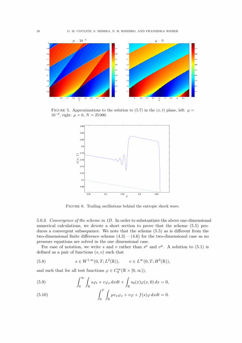
In order to check the possible convergence as µ → 0, we computed approximations withN = 25 000, and t ∈ [0, 1]. In Figure 5 we show the result in the (x, t) plane for µ =10−6 and µ = 0. The two solutions are identical until shocks develop at t ≈ 0.05.At this point the approximation with µ = 10−6 develop two shocks, the slower (andweaker) is an entropy satisfying shock wave, while the faster (and stronger) violates theentropy condition. From the figure it is visible how the characteristics “pass through”the shock. Of course, if µ = 0 the scheme reduces to the Lax-Friedrichs scheme, andthe approximation to the right is close to the entropy solution. The small entropic shockwave cannot be a traveling wave solution, whereas the large non-entropic shock wave is,since it is symmetric about s = 1/2. This follows from the previous analysis, and can beseen by the trailing oscillations in the small shock, these are absent in the large shock,see Figure 6.

Remark 5.1. The above simulations clearly indicate that the µ → 0 limit for the Brinkmanregularization results in a non-classical shock (see [16] for definition) of the limit conser-vation law (st+f(s)x = 0). Such non-classical shocks in the context of two-phase flows inone-dimensional porous media also arise in the models with dynamic capillary pressure,see [12, 11, 7]. It is interesting to observe that non-classical shock waves for two-phaseflows can arise with two very different regularization mechanisms, one involving dynamiccapillary pressure and one with a Brinkman regularization of the Darcy’s law.


Figure 5. Approximations to the solution to (5.7) in the (x, t) plane, left: µ =10−6, right: µ = 0, N = 25 000.

0.45 0.5 0.55 0.6 0.65

0.68

0.7

0.72

0.74

0.76

0.78

0.8

0.82

0.84

0.86

x

s(x

,1)

Figure 6. Trailing oscillations behind the entropic shock wave.

5.0.3. Convergence of the scheme in 1D. In order to substantiate the above one-dimensionalnumerical calculations, we devote a short section to prove that the scheme (5.5) pro-duces a convergent subsequence. We note that the scheme (5.5) as is different from thetwo-dimensional finite difference scheme (4.3) – (4.6) for the two-dimensional case as nopressure equations are solved in the one dimensional case.

For ease of notation, we write s and v rather than sµ and vµ. A solution to (5.1) isdefined as a pair of functions (s, v) such that

(5.8) s ∈ W 1,∞(0, T ;L2(R)), v ∈ L∞(0, T ;H2(R)),

and such that for all test functions ϕ ∈ C∞0 (R× [0,∞)),

∫ ∞

0

∫

R

sϕt + vϕx dxdt+

∫

R

s0(x)ϕ(x, 0) dx = 0,(5.9)

∫ T

0

∫

R

µvxϕx + vϕ+ f(s)ϕdxdt = 0.(5.10)


Using the obvious notation, (5.5) reads

(5.11)

D+t s

nj +Dcv

nj = 0,

µD+D−vnj + vnj = f(snj ).

s0j = s0(j∆x), for j ∈ Z.

From the discrete values we define the bilinear interpolant

sn(x) = snj + (x− xj)D+snj for x ∈ [xj , xj+1),

s∆x(x, t) = sn(x) + (t− tn)D+t s

n(x) for t ∈ [tn, tn+1).

Regarding vnj , we define vn(x) to be the piecewise quadratic spline interpolation such that

vn(xj) = vnj , and define v∆x(x, t) by a linear interpolation in t between tn and tn+1.Since this scheme is conservative, it follows that if s∆x → s, v∆x → v and ∂xv∆x → ∂xv

a.e. as ∆x → 0, then the limits s and v satisfy (5.9) and (5.10) respectively.In order to show the strong convergence of a subsequence we square the equation for

vnj and sum over j to find

µ2∑

j

∣∣D−D+v

nj

∣∣2 + 2µ

∑

j

∣∣D−v

nj

∣∣2 +

∑

j

∣∣vnj

∣∣2 =

∑

j

∣∣fn

j

∣∣2 .

This means that(5.12)

∥∥∂2

xv∆x(·, t)∥∥2

L2(R)+ ‖∂xv∆x(·, t)‖2L2(R) + ‖v∆x(·, t)‖2L2(R) ≤ C ‖f‖2Lip ‖s∆x(·, t)‖2L2(R) ,

for some constant C which does not depend on ∆x. Next, we note that

‖s∆x(·, tn+1)‖L2(R) ≤ ‖s∆x(·, tn)‖L2(R) + C∆t ‖∂xv∆x(·, tn)‖L2(R)

≤ ‖s∆x(·, tn)‖L2(R)

(

1 + C∆t ‖f‖Lip)

.

Thus

(5.13) ‖s∆x(·, t)‖L2(R) ≤ ‖s0‖L2(R) eCt,

for some constant C which does not depend on ∆x (but scales like 1/µ). Combining thiswith (5.12) we find that

(5.14) ‖v∆x(·, t)‖H2(R) ≤ CT

for all t ≤ T . This means that we get a supremum bound on s∆x, since

‖∂xv∆x‖L∞(R) ≤ ‖v∆x‖H2(R) .

Therefore

(5.15) ‖s∆x(·, t)‖L∞(R) ≤ ‖s0‖L∞(R) + tCT .

In particular, this implies that we only have to demand that f is locally Lipschitz contin-uous.

Now set rnj = D+t s

nj and znj = D+

t vnj . Then

D+t r

nj +Dcz

nj = 0,

−µD+D−znj + znj = f ′

(

sn+1/2j

)

rnj ,n ≥ 0,

where sn+1/2j is some value between snj and sn+1

j . The above holds for n ≥ 0, and we havethat

r0j = −Dcv0j , or − µD+D−r

0j + r0j = −f ′

(s0j)Dcs

0j ,


where s0j is a value between s0j−1 and s0j+1. Now we can repeat the above arguments toshow that

‖∂tv∆x(·, t)‖H2(R) ≤ C ‖f‖Lip ‖∂ts∆x(·, t)‖L2(R) ,(5.16)

‖∂ts∆x(·, t)‖L2(R) ≤ ‖f‖Lip ‖∂xs0‖L2(R) eCt.(5.17)

Thus, if s0 ∈ H1(R), then s∆x ∈ Lip(0, T ;L2(R)) and v∆x ∈ Lip(0, T ;H2(R)), withLipschitz constants independent of ∆x.

Now we need to show the compactness of the two sequences s∆x∆x>0 and v∆x∆x>0.Set σn

j = D−snj and wn

j = D−vnj , then

D+t σ

nj +Dcw

nj = 0,

−µD+D−wnj + wn

j = f ′(

snj−1/2

)

σnj ,

n ≥ 0,

where snj−1/2 is an intermediate value. The initial values for the above scheme are σ0j =

D−v0j . From this we obtain

‖∂xv∆x(·, t)‖H2(R) ≤ C ‖f‖Lip ‖∂xs∆x(·, t)‖L2(R) ,(5.18)

‖∂xs∆x(·, t)‖L2(R) ≤ ‖f‖Lip ‖∂xs0‖L2(R) eCt.(5.19)

Therefore s∆x(·, t)∆x>0 ⊂ H1(R) ⊂⊂ L2(R) and v∆x(·, t)∆x>0 ⊂ H3(R) ⊂⊂ H2(R)uniformly in t and ∆x.

To sum up, we have proved

Lemma 5.1. Assume that s0 ∈ H1(R) and that s∆x and v∆x are defined by (5.11). Thenthere are functions s and v that are weak solutions to (5.1), defined by (5.8), (5.9) and(5.10). We have that

s∆x(·, t) → s(·, t) in L2(R),

v∆x(·, t) → v(·, t) in H2(R),along a subsequence

for all t ∈ [0, T ].

6. Conclusion

Two-phase flows in a porous medium is modeled by a hyperbolic equation for thesaturation, coupled with an elliptic equation for the pressure, resulting in the classicalDarcy’s law based equations (1.9). No existence results for the equations have beenobtained till date in spite of the extensive research on these equations over the past severaldecades. One of the pressing issues in this context has been whether the Darcy’s law is anadequate and appropriate model for flows in porous media. The Brinkman regularizationof the Darcy’s law [4] has been a popular alternative ([15] and references therein) for theDarcy’s law in the geophysics community, atleast in the context of a single phase flow. Itis natural to examine whether the Brinkman regularization is an appropriate model, alsoin the context of two- (and multi-) phase flows in porous media.

In this paper, we consider the Brinkman regularization of the two-phase flow equations(1.12). A suitable notion of weak solutions for these equations is proposed. We prove thatthese weak solutions exist. Furthermore, a simple finite difference scheme to approximatethis system (1.12) is proposed and is shown to converge to the weak solutions. Numericalexperiments indicate robust performance of this numerical scheme, for fixed regularizationparameter µ.

Formally, we can recover the classical two-phase flow equations (1.9) by setting theregularization parameter µ → 0 in the Brinkman regularization (1.12). However, our


stability estimates on the saturation and the velocity blow up as µ → 0 preventing usfrom rigorously showing that the limit solution of the Brinkman regularization is a weaksolution of the classical Darcy problem. We investigate this question numerically usingour convergent numerical scheme. Results on a benchmark quarter five-spot problem intwo space dimensions show that the approximate solutions to the Brinkman regulariza-tion can become quite oscillatory as µ → 0. Furthermore, the regularized system cancontain discontinuous fronts connecting full water saturation to zero water saturation.Such solutions are not included as classical entropy solutions of the Darcy problem (1.12).Hence, the numerical results indicate that the Brinkman regularization may not convergeto (entropy solutions of) the Darcy limit as µ → 0.

This proposition is further investigated in the special case of one space dimension. Inthis case, the pressure equation is trivially solved and the saturation is modeled by a scalarconservation law. Entropy solutions (obeying Lax type entropy conditions) are widelyrecognized as the physically relevant solutions in this context. However, we establishusing traveling wave analysis that the Brinkman limit will lead to a non-classical shockwave for the scalar conservation law. Such non-entropic solutions have been postulated forother physical models such as dynamic capillary pressure models [12, 11]. The presenceof non-classical shocks for the Brinkman limit raise interesting questions, see also [9].

Summarizing, the Brinkman regularization does provide a model where existence ofweak solutions can be shown rigorously and convergent numerical schemes can also bedesigned. Such existence and convergence results have not been possible for the Darcyproblem despite several attempts. On the other hand, the Brinkman regularization maylead to limit solutions of the Darcy’s equation that are not entropic and may contain non-classical shock waves. Furthermore, the question of rigorous passage to the Darcy limitfor the Brinkman regularization is still wide open. Hence, this paper advocates caution inthe use of Brinkman type models, atleast for two and multi-phase flows in porous media.

References

[1] Adimurthi, S. Mishra, and G. D. Veerappa Gowda. Optimal entropy solutions for scalar conservation lawswith discontinuous flux. J. Hyperbolic. Diff. Eqns., 2(4), 787-838, 2005.

[2] B. Andreianov, K. H. Karlsen, and N. H. Risebro. A theory of L1 dissipative solvers for scalar conservationlaws with discontinuous flux. Arch. Ration. Mech. Anal. 201(1) (2011), 27-86.

[3] K. Aziz and A. Settari. Petroleum reservoir simulation. Applied Science Publisher, London, 1979.[4] H. C. Brinkman Calculation of the viscous force exerted by a flowing fluid on a dense swarm of particles.

Applied Scientific Research section a- Mechanics Heat Chemical Engineering Mathematical Methods, 1(1),27-34, 1947.

[5] G. M. Coclite, K. H. Karlsen, S. Mishra, and N. H. Risebro. A hyperbolic-elliptic model for two phaseflows in porous media- existence of entropy solutions. Int. J. Numer. Anal. Model. 9 (2012), no. 3, 562583

[6] G. M. Coclite, S. Mishra, and N. H. Risebro. Convergence of an Engquist-Osher scheme for a multi-dimensional triangular system of conservation laws. Math. Comput., 79 (269), 71-94, 2010.

[7] G. M. Coclite, L. DiRuvo, J. Ernest and S. Mishra. Convergence of vanishing capillarity approximations

for scalar conservation laws with discontinuous fluxes. Research report NN. 2012-30, SAM ETH Zurich.[8] C. Dafermos. Hyperbolic conservation laws in continuum physics. Springer, Berlin, 2000.

[9] T. Elperin, N. Kleeorin and A. Krylov Nondissipative shock waves in two-phase flows. Physica D., 74,372-385, 1994.

[10] T. Gimse and N. H. Risebro. Solution of the Cauchy problem for a conservation law with discontinuous fluxfunction. SIAM J. Math. Anal., 23(3), 635-648, 1992.

[11] R. Helmig, A. Weiss and B. I. Wohlmuth. Dynamic capillary effects in heterogeneous porous media. Comp.Geosci. 11 (2007), 261-274.

[12] S. Hassanizadeh and W. G. Gray. Mechanics and thermodynamics of multiphase flow in porous media includinginterphase boundaries. Adv. Wat. Res. 13 (4) (1990), 169-186.

[13] K. H. Karlsen, N. H. Risebro, and J. D. Towers. L1 stability for entropy solutions of degenerate parabolic

convection-diffusion equations with discontinuous coefficients. Skr. K. Nor. Vidensk. Selsk., 3, 1-49, 2003.[14] S. N. Kruzkov and S. M. Sukorjanskiı. Boundary value problems for systems of equations of two phase

filtration type; formulation of problems, questions of solvability, justification of approximate methods. Mat.

Sb. (N.S.), 104(146)(1), 69-88, 1977.


[15] M. Krotkiewski, I. Ligaarden, K-A. Lie and D.W. Schmid. On the importance of the Stokes-Brikmanequations for computing effective permeability in carbonate-karst reservoirs. Comm. Comput. Phys., 10 (5),1315-1332, 2011.

[16] P. LeFloch. Hyperbolic systems of conservation laws: the theory of classical and non-classical shock waves.Lecture notes in Mathematics., ETH Zurich, Birkhauser, 2002.

[17] S. Lukkhaus and P. I. Plotnikov. Entropy solutions of Buckley-Leverett equations. Siberian Math. J., 41(2),

329-348, 2000.[18] E. Marusic-Paloka, I. Pazanin, S. Marusic Comparison between Darcy and Brinkman laws in a fracture.

Appl. Math. Comput. 228 (14), 7538-7545, 2012.[19] S. P. Neumann. Theoretical derivation of Darcy’s law. Acta Mechanica, 25 (3-4), 153-170, 1977.[20] F. Otto. Stability Investigation of Planar Solutions of Buckley-Leverett Equation. Sonderforchungbereich 256

[Preprint; No. 345] (1995).

(Giuseppe Maria Coclite)Department of Mathematics

University of Bari

via E. Orabona 4I–70125 Bari, Italy

E-mail address: [email protected]: http://www.dm.uniba.it/Members/coclitegm/

(Siddhartha Mishra)

Seminar for Applied Mathematics (SAM)ETH Zurich,HG G 57.2, Ramistrasse 101, Zurich, Switzerland.

E-mail address: [email protected]: http://folk.uio.no/siddharm/

(Nils Henrik Risebro)Centre of Mathematics for Applications (CMA)University of OsloP.O. Box 1053, BlindernN–0316 Oslo, Norway

E-mail address: [email protected]: http://www.math.uio.no/~nilshr/

(Franziska R. Weber)

Centre of Mathematics for Applications (CMA)University of Oslo

P.O. Box 1053, Blindern

N–0316 Oslo, NorwayE-mail address: [email protected]

Recent Research Reports

Nr. Authors/Title

2013-34 M. Hutzenthaler and A. Jentzen and X. WangExponential integrability properties of numerical approximation processes fornonlinear stochastic differential equations

2013-35 S. Cox and M. Hutzenthaler and A. JentzenLocal Lipschitz continuity in the initial value and strong completeness for nonlinearstochastic differential equations

2013-36 S. Becker and A. Jentzen and P. KloedenAn exponential Wagner-Platen type scheme for SPDEs

2013-37 D. Bloemker and A. JentzenGalerkin approximations for the stochastic Burgers equation

2013-38 W. E and A. Jentzen and H. ShenRenormalized powers of Ornstein-Uhlenbeck processes and well-posedness ofstochastic Ginzburg-Landau equations

2013-39 D. Schoetzau and Ch. Schwab and T.P. Wihlerhp-dGFEM for Second-Order Mixed Elliptic Problems in Polyhedra

2013-40 S. Mishra and F. Fuchs and A. McMurry and N.H. RisebroEXPLICIT AND IMPLICIT FINITE VOLUME SCHEMES FOR

RADIATION MHD AND THE EFFECTS OF RADIATION ON

WAVE PROPAGATION IN STRATIFIED ATMOSPHERES.

2013-41 J. Ernest and P. LeFloch and S. MishraSchemes with Well controlled Dissipation (WCD) I: Non-classical shock waves

analysis and numerical approximation of brinkman ...€¦ · analysis and numerical approximation...

Documents